Embed Size (px)
Citation preview

Distances and automatic sequences indistinguished variants of Hanoi graphs
Caroline Holz auf der Heide
Dissertation
an der Fakultät für Mathematik, Informatik und Statistik
der Ludwig-Maximilians-Universität München
vorgelegt von
Caroline Holz auf der Heide
am 24. August 2016

1. Gutachter: Prof. Dr. Andreas M. Hinz(Ludwig-Maximilians-Universität München)
2. Gutachter: Prof. Jean-Paul Allouche(CNRS, Institut de Mathématiques de Jussieu-PRG,Université Pierre et Marie Curie)
Tag der mündlichen Prüfung: 7. Dezember 2016

Abstract
In this thesis three open problems concerning Hanoi-type graphs are addressed. I prove atheorem to determine all shortest paths between two arbitrary vertices s and t in the generalSierpinski graph S n
p with base p ≥ 3 and exponent n ≥ 0 and find an algorithm based on thistheorem which gives us the index of the potential auxiliary subgraph, the distance between sand t and the best first move(s). Using the isomorphism between S n
3 and the Hanoi graphs Hn3 ,
this algorithm also determines the shortest paths in Hn3 . The results are also used in order to
simplify proofs of already known metric properties of S np. Additionally, I compute the aver-
age number of input pairs (si, ti) for i ∈ {1, . . . , n} to be read by the algorithm. The theoremand the algorithm for S n
p are modified for the Sierpinski triangle graphs, which are deeplyconnected to the well-known Sierpinski triangle and the Sierpinski graphs, with the resultthat the shortest paths in the Sierpinski triangle graphs can be determined for the first time.The Hanoi graphs Hn
3 are then considered as directed graphs by differentiating the directionsof the disc moves between the pegs of the corresponding Tower of Hanoi. For the problem totransfer a tower from one peg to another peg there are five different solvable variants. Here,the variants T H(C+
3 ) and T H(K−3 ) are discussed concerning the infinite sequences of moveswhich arise from the solutions as n tends to infinity. The Allouche-Sapir Conjecture saysthat these sequences are not d-automatic for any d. I prove this for the T H(C+
3 ) sequencewith the aid of the frequency of a letter and its rationality in automatic sequences. For theT H(K−3 ) sequence I employ Cobham’s Theorem about multiplicative independence, auto-matic sequences and ultimate periodicity. I show that this sequence is the image, under a1-uniform morphism, of an iterative fixed point of a primitive prolongable endomorphism.F. Durand’s methoda is then used for the decision about the question whether the sequence isultimately periodic. The method of I. V. Mitrofanovb, which works with subword schemata,is applied to the problem as well. Using the theory of recognisable sets, a sufficient conditionfor deciding the question about the automaticity of the T H(K−3 ) sequence is deduced.Finally, a yet not studied distance problem on the so-called Star Tower of Hanoi, which isbased on the star graph S t(4), is considered. Assuming that the Frame-Stewart type strategy isoptimal, a recurrence for the length of the resulting paths is deduced and solved up to n = 12.
a F. Durand, HD0L ω-equivalence and periodicity problems in the primitive case (to the memory of G. Rauzy).Journal of Uniform Distribution Theory, 7(1):199-215, 2012
b I. V. Mitrofanov, Periodicity of Morphic Words, Journal of Mathematical Sciences, 206(6):679-687, 2015


Zusammenfassung
Ich beweise ein Theorem zur Bestimmung aller kürzesten Wege zwischen zwei beliebigenEcken s und t in den allgemeinen Sierpinski-Graphen S n
p mit Basis p ≥ 3 und Exponentn ≥ 0 und erstelle auf diesem Theorem beruhend einen Algorithmus, der den Index des all-fälligen Hilfsuntergraphen, den Abstand zwischen s und t und einen besten ersten Schrittliefert. Unter Verwendung des Isomorphismus zwischen S n
3 und den Hanoi-Graphen Hn3
bestimmt dieser Algorithmus auch die kürzesten Wege in Hn3 . Die Ergebnisse werden be-
nutzt, um Beweise bereits bekannter metrischer Eigenschaften der S np zu vereinfachen. Zu-
sätzlich berechne ich die durchschnittlich benötigte Anzahl von Eingabepaaren (si, ti) füri ∈ {1, . . . , n} in den Algorithmus. Das Theorem und der Algorithmus für S n
p werden fürdie Klasse der Sierpinski-Dreiecksgraphen, welche in direktem Zusammenhang mit dem be-rühmten Sierpinski-Dreieck und den Sierpinski-Graphen stehen, modifiziert, sodass erstmalsauch die kürzesten Wege in diesen Graphen bestimmt werden können.Die Hanoi-Graphen Hn
3 werden dann als gerichtete Graphen betrachtet, indem man die Rich-tungen der Bewegungen zwischen den Stäben des entsprechenden Turms von Hanoi diffe-renziert. Für das Problem des Versetzens eines Turms von einem Stab auf einen anderen gibtes fünf verschiedene lösbare Varianten. Die Varianten T H(C+
3 ) und T H(K−3 ) werden bezüg-lich der unendlichen Folgen von Bewegungen betrachtet, die sich durch die Lösung für ngegen Unendlich strebend ergeben. Die Allouche-Sapir-Vermutung besagt, dass für kein ddiese Folgen d-automatisch erzeugt sind. Ich beweise dies für die T H(C+
3 ) Folge mit Hil-fe der Theorie über die Häufigkeit eines Buchstabens und deren Rationalität in automatischerzeugten Folgen. Für die T H(K−3 ) Folge wird Cobhams Theorem über multiplikative Un-abhängigkeit, automatisch erzeugte Folgen und ultimative Periodizität verwendet. Ich zeige,dass diese Folge das Bild, unter einem 1-uniformen Morphismus, eines iterativen Fixpunk-tes eines primitiven verlängerbaren Endomorphismus ist. Die Methode von F. Duranda wirddann für die Entscheidung über die Frage, ob die Folge ultimativ periodisch ist, verwendet.Ebenso wird die Methode von I. V. Mitrofanovb, welche mit Teilwortschemata arbeitet, aufdas Problem angewandt. Unter Verwendung der Theorie über erkennbare Mengen wird einehinreichende Bedingung für die Frage der Automatizität der T H(K−3 ) Folge hergeleitet.Zuletzt wird ein bislang nicht untersuchtes Abstandsproblem im sogenannten Stern-Turm-von-Hanoi betrachtet, welcher auf dem Stern-Graphen S t(4) beruht. Unter der Annahme,dass die Frame-Stewart-Strategie optimal sei, wird eine Rekursionsvorschrift für die Längeder so gewonnenen Wege entwickelt und bis n = 12 gelöst.
a F. Durand, HD0L ω-equivalence and periodicity problems in the primitive case (to the memory of G. Rauzy).Journal of Uniform Distribution Theory, 7(1):199-215, 2012
b I. V. Mitrofanov, Periodicity of Morphic Words, Journal of Mathematical Sciences, 206(6):679-687, 2015


Acknowledgements
It is my pleasure to acknowledge a number of people who contributed towards the successfulcompletion of my thesis.
First and foremost, my sincerest gratitude goes to my supervisor Prof. Andreas M. Hinz forall his help, his support and trust during my doctorate years and before, and for giving methe scientific freedom to develop the ideas that are presented in this thesis. Our conversationsinspired me and were very precious to me. I am thankful to him for providing me the op-portunity to visit the University of Maribor that helped me to broaden my knowledge and tomeet other researchers. I feel honoured to have worked with him.
I also want to acknowledge my great debt to Jean-Paul Allouche for providing me with sup-port for the second part of this thesis and for accepting to be my second supervisor and amember of the doctoral committee. I thank him for encouraging me to apply to the Summerschool “CombinatoireS” which gave me the opportunity to expand my horizons in the fieldof combinatorics. It is my honour to have met him and discussed mathematics with him.
Besides my supervisors, I would like to thank my doctoral committee including Prof. Kon-stantinos Panagiotou and Prof. Daniel Rost.
I owe special thank to Prof. Sandi Klavžar, Prof. Boštjan Brešar, Ciril Petr and the othermembers of the Faculty of the Natural Sciences and Mathematics of the University of Mariborfor the fruitful intellectual exchange.
I am deeply grateful to my family, particularly my parents, for their support, humour and helpduring completion of my thesis and in my life in general and for their unwavering belief inme.
Weyarn, August 2016 Caroline Holz auf der Heide


Contents
0 Introduction 1
1 A P2 decision algorithm for Sierpinski graphs with base p ∈ N3 71.1 The isomorphism between the Hanoi graphs Hn
3 and the Sierpinski graphs S n3 . . 8
1.2 A P2 decision automaton for S n3 - D. Romik’s Automaton . . . . . . . . . . . . . 11
1.3 Sierpinski graphs S np with base p ∈ N and exponent n ∈ N0 . . . . . . . . . . . . 17
1.4 A P2 decision algorithm for Sierpinski graphs S np with base p ∈ N3 and
exponent n ∈ N0 . . . . . . . . . . . . . . . . . . . . . . . . . . . . . . . . . . . 221.4.1 The underlying principle . . . . . . . . . . . . . . . . . . . . . . . . . . 231.4.2 The P2 decision algorithm . . . . . . . . . . . . . . . . . . . . . . . . . 311.4.3 Some applications . . . . . . . . . . . . . . . . . . . . . . . . . . . . . 331.4.4 The average number of pairs to be read to solve the problem . . . . . . . 36
1.5 An algorithm to determine the shortest paths in Sierpinski triangle graphs S T np
with base p ∈ N3 and exponent n ∈ N0 . . . . . . . . . . . . . . . . . . . . . . . 381.5.1 A P2 decision algorithm for Sierpinski triangle graphs S T n
3 . . . . . . . . 411.5.2 A P2 decision algorithm for Sierpinski triangle graphs S T n
p withbase p ∈ N3 . . . . . . . . . . . . . . . . . . . . . . . . . . . . . . . . . 45
1.6 Conclusion and Outlook . . . . . . . . . . . . . . . . . . . . . . . . . . . . . . 49
2 Variations on the Tower of Hanoi with 3 pegs 532.1 Words, morphisms, and sequences . . . . . . . . . . . . . . . . . . . . . . . . . 562.2 An approach to disprove the automaticity of the T H(C+
3 ) and theT H(K−3 ) sequences based on the frequency of a letter . . . . . . . . . . . . . . . 592.2.1 Necessary tools . . . . . . . . . . . . . . . . . . . . . . . . . . . . . . . 602.2.2 The T H(C+
3 ) sequence . . . . . . . . . . . . . . . . . . . . . . . . . . . 662.2.3 The T H(K−3 ) sequence . . . . . . . . . . . . . . . . . . . . . . . . . . . 73
2.3 A new approach to disprove the automaticity of the T H(K−3 ) sequence . . . . . . 792.3.1 F. Durand’s method about the ultimate periodicity of (primitive) sequences 822.3.2 Ultimate periodicity and subword schemes using I. V. Mitrofanov’s method 90
2.4 Conclusion and Outlook . . . . . . . . . . . . . . . . . . . . . . . . . . . . . . 99
3 The Star Tower of Hanoi: a variant of the Tower of Hanoi with 4 pegs 101
Bibliography 111
I

Symbol Index
d(s, t) distance between vertices sand t, 10
diam(G) diameter of graph G, 20
E(G) edge set of graph G, 7
E(ψ) limit matrix ofM(ψ)n
n jλr(ψ)n , 63
Freqa(s) frequency of letter a in se-quence s, 60
Hn3 Hanoi graph (with base 3), 8
J Jordan matrix, 61
Ji Jordan block, 61
J(ψ) Jordan form of M(ψ), 63
M(ψ) incidence matrix of morphismψ, 57
P0 problem perfect to perfect, 7
P1 problem regular to perfect, 7
P2 problem regular to regular, 7
per(I) period of state I, 83
repd(n) base-d expansion of n, 98
S n3 Sierpinski graph (with base
3), 7
S np general Sierpinski graph, 17
s sequence, 56
s[i] si for sequence s, 56
s[i... j] sisi+1 . . . s j for sequence s, 56
Spec(M) spectrum of matrix M, 96
S T n3 Sierpinski triangle graph
(with base 3), 41
S T np Sierpinski triangle graph, 39
S t01 number of moves in Star THfrom central peg to externalpeg, 105
S t01 number of moves in Star THfrom central peg to externalpeg using Frame, 105
S t10 number of moves in Star THfrom external peg to centralpeg, 105
S t10 number of moves in Star THfrom external peg to centralpeg using Frame, 105
S t12 number of moves in Star THfrom external peg to externalpeg, 102
S t(p) (directed) star depending onp ∈ N, 101
T set {0, 1, 2}, 2
u T H(K−3 ) sequence, 73
V(G) vertex set of graph G, 7
W(τ, ψ) matrix M(τ)E(ψ), 65
w T H(C+3 ) sequence, 66
∆C+ set {a, b, c, a}, 66
∆K− set {a, b, c, a, b}, 73
ε empty word, 56
ε(G) average eccentricity of graphG, 20
εG(s) eccentricity of vertexs ∈ V(G), 20
III

η morphism corresponding tow, 66
κ coding corresponding tow, 66
λr Perron-Frobenius eigen-value, 61
ρ(M) spectral radius of matrixM, 96
Σ∗ set of finite words on alphabetΣ, 56
ΣC+ set {x, r, z, t, u, s, a, b, c, a}, 66
ΣK− set{x, y, z, d, e, f , a, b, c, a, b
}, 73
τ coding corresponding to u, 73
φ morphism corresponding tou, 73
ψ∞(a) (iterative) fixed point ofmorphism ψ on letter a, 58(
nk
)combinatorial number, 19(
Sk
)set of all subsets of S of sizek, 19
||G|| size of set E(G) for graphG, 18
i4 j binary operation defined onT , 10
k primitive vertex in S T np, 39
|M| size of set M, 11
N set {1, 2, 3, . . .}, 3
Nk set {k, k + 1, . . .}, 3
[n]0 set {0, . . . , n − 1}, 7
[n] set {1, . . . , n}, 7
[n]2 set {2, . . . , n}, 7
|s| length of word s, 56
|s|a number of occurrences of let-ter a in word s, 56
(s4 j) best first move vector, 10
[S] binary truth value of state-ment S, 10
S(S ,T ) subword scheme for orderedsets of finite words S andT , 92
IV

Chapter 0
Introduction
It was in 1883 when François Édouard Anatole Lucas introduced a new puzzle1 motivated bythe following legend which was developed by H. de Parville [22] and translated into English byW. W. R. Ball ([11, p.228 f]):
“In the great temple at Benares, beneath the dome which marks the centreof the world, rests a brass plate in which are fixed three diamond needles,each a cubit high and as thick as the body of a bee. On one of these needles,at the creation, God placed sixty-four discs of pure gold, the largest discresting on the brass plate, and the others getting smaller and smaller up tothe top one. This is the Tower of Bramah. Day and night unceasingly thepriests transfer the discs from one diamond needle to another according tothe fixed and immutable laws of Bramah, which require that the priest onduty must not move more than one disc at a time and that he must placethis disc on a needle so that there is no smaller disc below it. When thesixty-four discs shall have been thus transferred from the needle on whichat the creation God placed them to one of the other needles, tower, temple,and Brahmins alike will crumble into dust, and with a thunderclap the worldwill vanish.”
Lucas marketed the game with only eight discs under the pseudonym N. Claus de Siam which isan anagram of Lucas d’Amiens. As name for his new puzzle he chose “La Tour d’Hanoï” (“TheTower of Hanoi”), since at this time Hanoi was in the headlines of French newspapers. Between1883 and 1885 the Sino-French war took place, among others in Tongkin, the northernmost partof what is now Vietnam. The name Tongkin is the corruption of Ðông Kinh, the name of Hanoiduring the Lê dynasty. Under French influence Hanoi was made the capital of this region. MaybeLucas chose the name “The Tower of Hanoi” to promote the selling of his game. Lucas was bornon 4 April 1842 in Amiens, in the north of France. Besides the Tower of Hanoi, he presented many
1According to Lucas, it was published in 1882 by himself, but one cannot find an evidence for this ([33]).
1

2 §0 Introduction
other puzzles like the Chinese Rings in his publications about Recreational Mathematics [60]. Buthe is also known for results in number theory, for instance the Lucas numbers2 and the proof thatthe Mersenne number 2127 − 1 is prime. In 1891, Lucas participated in a banquet of the congressof the “Association française pour l’avancement des sciences", of which he was an active member.During this event, a servant dropped a pile of plates and a piece of porcelain flew up and hit thecheek of Lucas which caused a deep wound. A few days later, on 3 October 1891, he died as aresult of this injury. The tomb can be found on the Montmartre cemetery of Paris ([36]).
Figure 0.1: The tomb of Édouard Lucas on the Montmartre cemetary, Paris:770cp1857, 23rd division, 8th row, 27 Avenue des Carrieres
c© 2015 C. Holz auf der Heide
Following the legend, the Tower of Hanoi consists of three needles, afterwards called pegs andnumbered with 0, 1, 2 such that T = {0, 1, 2} is the set of pegs, and a number of discs of increasingsize. To transfer one disc, you have to follow the divine rule that you “must place this disc on aneedle so that there is no smaller disc below it”. Lucas also stated the famous recursive solutionof the puzzle for an arbitrary number of discs ([33]). We explain it by an example. Assuming onecan solve the puzzle for four discs, then one can solve it for five discs as well since one transfersfirst the upper four discs to the non-goal peg, then the fifth disc to the goal peg and finally thefour discs from the non-goal peg to the goal peg. The recursive solution needs 2n − 1 moves totransfer a tower of n discs ([33]). For the number of discs in the legend, namely 64, we would need
2The Lucas numbers 2, 1, 3, 4, 7, 11, 18, . . . (OEIS AE000032) use the same recurrence relation as the famous Fibon-acci numbers (OEIS AE000045) (but starting with 2 and 1) and are closely related to these. Lucas studied both ofthem.

§0 Introduction 3
incredible 18 446 744 073 709 551 615 moves. Surprisingly, the minimality proof of the recursivealgorithm was lacking until 1981, when D. Wood [81, Theorem] gave one (cf. [33, pp. 44-45]for a deeper discussion). R. Olive found an algorithm which gives the moving disc in an optimalsolution, i.e., the solution with the minimum number of moves, of the Tower of Hanoi for the casethat we transfer a tower from one peg to another ([33, pp. 74–75]). The tasks on the tower werelater categorised in three classes of problems, first the case that we transfer a tower from one pegto another (P0), second the case that we transfer discs from an arbitrary regular state to a selectedpeg (P1) and last the case that we transfer discs from an arbitrary regular state to another regularstate (P2). To study the last class, use was made of the Hanoi graphs Hn
3 , first considered byScorer et al. [75], for n discs and 3 pegs. Initially, a distance on these graphs was determined forthe second class of problems [34]. It turned out that the diameter of Hn
3 is equal to the distancebetween two perfect vertices. For the moves of the largest disc the following result, named theboxer rule [33], was proved. If on a shortest path between two vertices the largest disc once movesaway from a peg, it will not return to the same peg.D. Romik [70] then gave an algorithm, based on what has become known as “Romik’s auto-maton”, to determine the distance in the third class of problems. He used for the proof anotherclass of graphs, the Sierpinski graphs. This was possible as the Sierpinski graphs S n
3 for 3 pegsare a variant of the Hanoi graphs Hn
3 , more precisely they are isomorphic ([52], [70]). This variantof the Hanoi graphs is named after the famous Sierpinski triangle because of their deep connec-tion which was found by A. M. Hinz and A. Schief ([33, Section 4.3], [42]). These graphs canbe interpreted as state graphs of a variant of the Tower of Hanoi puzzle, the Switching Towerof Hanoi ([52]). S. Klavžar and U. Milutinovic generalised the graphs in [52] to the Sierpinskigraphs S n
p with base p ∈ N and exponent n ∈ N0. Here, we introduce the notation Nk for allwhole numbers k such that Nk is the set of all whole numbers greater than or equal to k. ThenN0 = {0, 1, 2, . . .} and N1 = {1, 2, 3, . . .}, whereby we refer to N1 by N. The general Sierpinskigraphs were studied, inter alia, concerning their metric properties in [68], their distances betweenspecial vertices in [52], [54], and [82] and their average eccentricity in [41]. Some properties ofthe S n
3 or Hn3 , like the boxer rule, and the fact that for every non-extreme vertex of the graph there
is a vertex such there are two shortest paths between them, could be carried over to S np.
The book “The Tower of Hanoi —Myths and Maths” [33] by Hinz, Klavžar, Milutinovic andC. Petr, published in 2013, was the first to summarise the known results about the Tower of Hanoiand related topics. In the last chapter of this book [33, Chapter 9] open problems were stated. Oneof these problems was to “design an automaton analogous to Romik’s automaton for a “P2 task”in S n
p, p ≥ 4”3. Solving this problem is part of this thesis. We prove a new theorem aboutthe determination of the shortest path(s) for arbitrary vertices s and t in S n
p and design an al-gorithm which gives us the possible “detour” peg, the minimal distance and the best first move(s).Most of the results in an alternative representation were published by Hinz and the author of thepresent thesis in [37]. An overview on the Sierpinski graphs was given by Hinz, Klavžar andS. S. Zemljic [40]. This survey paper also covers the Sierpinski triangle graphs known fromL. L. Cristea and B. Steinsky [20], further studied by M. Jakovac [50] and again treated in [43].The theorem as well as the algorithm for the Sierpinski graphs can be extended to these newgraphs which will be done in the present work.
3 [33, p. 262]

4 §0 Introduction
One further problem listed in the last chapter of the book [33] was the subsequent conjecture aboutspecial variants of the Tower of Hanoi.
Conjecture 0.1 (Allouche-Sapir Conjecture). The two solvable Tower of Hanoi [variants] withoriented disc moves on three pegs that are not the Classical, the Cyclic, and the Linear Tower ofHanoi, are not d-automatic for any d.4
Let us describe what this means. The technical details, written in italics, will be explained in thelater chapters. We consider problems of P0 type. There are altogether five solvable variants ofthe Tower of Hanoi (TH) with 3 pegs, where one restricts the allowed orientation for disc moves.These are the Classical (T H(K3)), the Linear (T H(L3)), the Cyclic TH (T H(C3)), T H(C+
3 ), andT H(K−3 ), respectively. The state graphs of these variants are again variants of the Hanoi graphs,but with directed edges or arcs. The infinite sequence obtained from the moves of the solutionof the classical case as n goes to infinity was proved to be 2-automatic by J.-P. Allouche andF. Dress [5]. The Linear TH was mentioned for the first time in [75] by Scorer et al. and studiedin detail in [32] by H. Hering. The 3-automaticity of the infinite sequence corresponding to it wasthen shown by Allouche and A. Sapir [7]. Both proofs of automaticity used the algorithm whichwas given by Sapir [74] for solving recursively all these variants with the minimum number ofmoves. The Cyclic TH appeared in 1981 in [9], where M. D. Atkinson proposed an algorithm totransfer a perfect tower from peg 0 to peg 1. Other algorithms were given by different authors, forwhich we refer to [33, Chapter 8.2]. In 1994, Allouche [2] proved that the Cyclic TH sequence isnot d-automatic for any d ∈ N2. For the T H(C+
3 ) and the T H(K−3 ) sequence it was shown in [7]that they are morphic. But the question whether they are automatic remained open. The book [8]gives an overview on automatic sequences. In 1972, A. Cobham [18] proved that the frequencyof a letter in an automatic sequence, if it exists, is rational. Michel [61] showed in 1975 that ifa morphic sequence is primitive, then the frequency of all letters exists. K. Saari [71] then statedthat the frequency of letters exists for every pure binary morphic sequence. Later, in [72], he founda necessary and sufficient criterion for the existence and the value of the frequency of letters in amorphic sequence. Furthermore, he gave an if-and-only-if condition that all frequencies do in factexist. These results, which were not at the disposal of Allouche and Sapir, can be used to showthat certain sequences are not d-automatic for any d ∈ N as it is successfully done for the T H(C+
3 )sequence in the present thesis.For the T H(K−3 ) sequence we will make use of another theorem, known as Cobham’s Theorem [17],in the way that we want to prove whether the sequence is not ultimately periodic in order to an-swer the question of automaticity. The idea for this approach was already outlined in [7] andagain discussed during a private communication between Allouche and the author of the presentwork [3]. Morphic sequences are known in the theory of L-systems as HD0L sequences. Hencethe problem to decide whether a morphic sequence is ultimately periodic is called the HD0L ul-timate periodicity problem. The decidability for D0L sequences was shown by J.-J. Pansiot [67]and T. Harju and M. Linna [31] and for automatic sequences by J. Honkala [45]. Later, Allouche,N. Rampersad, and J. Shallit [6] presented a simpler proof for automatic sequences. F. Durandanswered the question for primitive HD0L sequences in [25]. An equivalent formulation of theHD0L ultimate periodicity problem in terms of recognisable sets and abstract numeration systems
4 ibid

§0 Introduction 5
was given by Honkala and M. Rigo in [47]. For this formulation Honkala already showed in [45]the decidability in the restricted case of usual integer bases, i.e., for d-automatic sequences. Dur-and succeeded then in giving a positive answer to the general problem in [26]. At around the sametime, I.V. Mitrofanov gave another solution, first put on ArXiv [62]. Later, a simpler proof waspublished by him [63]. We will use both proofs, Durand’s as well as Mitrofanov’s, in order to tryto determine whether the T H(K−3 ) sequence is ultimately periodic.
The first extension of the Tower of Hanoi to four pegs was introduced by H. E. Dudeney [23].He described the problem in a story about the Reve, some pilgrims and a number of cheeses ofvarying size. Therefore, this puzzle is known as The Reve’s puzzle. A presumed optimal solutionto transfer a tower from one peg to another peg was given independently by B. M. Frame andJ. S. Stewart [76] in 1941. The claim that the Frame-Stewart algorithm is optimal is known asthe Frame-Stewart Conjecture. It was open until T. Bousch proved in 2014 the optimality of thealgorithm [13]. In The Reve’s puzzle itself the orientations of the disc moves are not restricted.But according to [30, p. 218] there exist 83 non-isomorphic strong digraphs, which represent theallowed moves, for variants of the TH with 4 pegs. In 1994, P. K. Stockmeyer [78] introducedone of these variants and called it the Star Tower of Hanoi (Star TH) because of the structure ofthe corresponding directed graph. It turned out that this puzzle is related to the Linear TH in theway that this is the “Star TH” with three pegs. He gave a presumed optimal algorithm with theminimising value to transfer a tower from an external peg to another external peg. Chappelon andMatsuura [15] extended this problem to more than four pegs by adding external pegs and gen-eralised the algorithm. They showed that realising the presumed optimal algorithm the minimalnumber of moves is given by the generalised Frame-Stewart numbers. Stockmeyer conjecturedthat his algorithm “makes the smallest number of moves among all procedures that solve the Starpuzzle”, which is as Stockmeyer’s Conjecture also part of the list in [33, Chapter 9]. A furtherobject of this thesis is to find a presumed optimal algorithm and the number of moves for thetransfer of a tower from the central peg to an external peg for the case of four pegs.
This dissertation comprises three chapters. In Chapter 1 we focus on the P2 decision algorithmfor Sierpinski graphs with base p ∈ N. First, we define the Sierpinski graphs S n
3 with base 3 andexponent n ∈ N0 and give the isomorphism between the Hanoi graphs Hn
3 and S n3. The theorem and
the automaton of Romik, which can be adapted for the use for Hn3 by employing the isomorphism,
is then presented for S n3. Furthermore, we generalise the Sierpinski graphs to the base p ∈ N and
give some statements concerning them, in particular the definition of the distance function andthat there are at most two shortest paths between any two vertices in S n
p. In the next section weformulate the main theorem of this chapter about shortest paths between arbitrary vertices in S n
pand find an algorithm with some conclusions as well as an analysis of the necessary pairs of inputfor a decision. Then an application of our algorithm to Sierpinski triangle graphs is given.Chapter 2 mainly covers the variants of the TH with 3 pegs which are determined by the digraphsC+
3 and K−3 and the question whether the corresponding sequences are d-automatic for any d ∈ N.At the beginning, we give a summary of the terminology of finite and infinite words or sequencesused in this work and introduce morphic and automatic sequences. The first approach to disprovethe automaticity consists of the application of [18, Theorem 6] about automaticity and the ration-ality of the frequency of a letter. For that purpose we define the frequency of a letter and describethe steps to the theorem which states an if-and-only-if condition for the existence of the frequency

6 §0 Introduction
and gives the value of the frequency if it exists. These steps are portrayed for the T H(C+3 ) sequence
and culminate in the theorem that this sequence is not d-automatic by showing that the frequenciesfor all letters are irrational. The same approach is then used to attack the T H(K−3 ) sequence. Butit turns out that we are unable to determine whether the frequency is rational. Hence we choose inthe following section another approach which makes use of Cobham’s Theorem about the ultimateperiodicity and automatic sequences. We present the results of Durand’s work about the decidab-ility of the ultimately periodicity problem for morphic and primitive morphic sequences as far asthey are useful for us and apply them to our problem. We find a primitive morphism and a codingsuch that the T H(K−3 ) sequence is a primitive morphic sequence and give an algorithm for thedetermination of a constant which we need to decide on the ultimate periodicity. In the last sub-section we introduce subword schemes, explain an algorithm which decides whether a sequenceis ultimately periodic with the aid of subword schemes, and apply the results on our sequence.Further, we analyse these subword schemes for our sequence and give a sufficient condition forthe d-automaticity of the T H(K−3 ) sequence using the theory of recognisable sets.In Chapter 3 we investigate the problem of finding a pattern in the number of moves for an in-creasing number of discs in the Star TH. First, we describe the presumed optimal solution for theP0 task from an external peg to another external peg by the Frame-Stewart strategy. After thatwe analyse the two different approaches of Frame and Stewart for a solution and the sequence ofmoves for the problem to transfer a tower from the central peg to an external peg. It will turn outthat both strategies give the same formula for the number of moves. We analyse the number ofmoves for different values of splitting and give the first values for the number of moves resultingfrom the algorithm with the minimising value of splitting.

Chapter 1
A P2 decision algorithm for Sierpinski graphswith base p ∈ N3
One very well-known variant of the Tower of Hanoi is the Switching Tower of Hanoi (SwitchingTH) with three pegs, labeled with 0, 1, and 2. Assume that we have n discs. Then a state s ∈ T n
is a legal distribution of n discs and written as s = sn . . . s1, where si ∈ T means that the i-th disclies on peg si. A state is regular if no larger disc lies on a smaller one. A regular state such that alldiscs lie on a single peg is called perfect.
The problem to transfer a perfect tower from one peg to another peg or to go from a perfect stateto a perfect state, respectively, in a minimum number of moves is called the problem of P0 type.If we want to go from a regular state to a perfect state, the problem is of P1 type. Consequently,the problem to go from a regular state to another regular state is called a problem of P2 type.
For n ∈ Nwe introduce the notation [n]0 for the set {0, . . . , n−1}, [n] for the set {1, . . . , n}, and [n]2
for the set {2, . . . , n}. The allowed moves to transfer the discs in the Switching TH with n ∈ N0
discs are as follows. Assume we have a regular state in which the d − 1 ∈ [n]0 topmost discs onpeg i are the d − 1 smallest ones. Then we can switch the d-th smallest disc on peg j , i with thed − 1 discs on i. That d − 1 = 0 is included, means that arbitrary moves of the smallest disc areallowed.
If we interpret the states as vertices and the moves as edges, we can define a graph G consisting ofV(G) and E(G), where V(G) is the vertex set and E(G) is the edge set. The graph associated withthe Switching TH is the Sierpinski graph S n
3 with base p = 3 and exponent n ∈ N0. Its vertex setis V(S n
3) = T n. The edges of S n3 are of the form
{si jd−1, s jid−1
}, where i, j ∈ T, i , j, d ∈ [n], and
s ∈ T n−d. Hence the edge set is
E(S n3) =
{{s jid−1, si jd−1
} ∣∣∣∣ i, j ∈ T, i , j, d ∈ [n], s ∈ T n−d}. (1.1)
The disc d is here the moving single disc in the move as described above with any distribution sof discs larger than d.
7

8 §1 A P2 decision algorithm for Sierpinski graphs with base p ∈ N3
There exists another definition of the edge set using the fact that S n+13 contains three subgraphs iS n
3,which are generated by the shift of the labels of one copy of S n
3 (see Figure 1.1 for n = 0, 1, 2).Then
E(S 03) = ∅,
∀n ∈ N0 : E(S n+13 ) =
{{is, is′}
∣∣∣∣ i ∈ T, {s, s′} ∈ E(S n3)}
∪ {{i jn, jin} | i, j ∈ T, i , j} .
(1.2)
1 0 2 1110 12 21 222001 00 02111 112110101100 102
121 122120 200201 202220222221210211 212022020021012011010 002000001
1
Figure 1.1: Sierpinski graphs S 13, S 2
3, and S 33
A comparison of Figures 1.1 and 1.2 imposes the question whether S n3 and the Hanoi graph Hn
3 areisomorphic for fixed n ∈ N. We will now clarify this.
1.1 The isomorphism between the Hanoi graphs Hn3 and the Sier-
pinski graphs S n3
In this section we want to show the existence of an isomorphism between the Sierpinski graphs S n3
and the Hanoi graphs Hn3 and some results about Hn
3 which can be transferred to Sierpinskigraphs S n
3 with the aid of the isomorphism. At first we will describe the vertex set V(Hn3) of
the Hanoi graph with base p = 3 and exponent n ∈ N0 and the edge set E(Hn3) :
V(Hn3) = T n,
E(Hn3) =
{{si(3 − i − j)d−1, s j(3 − i − j)d−1
} ∣∣∣∣ i, j ∈ T, i , j, d ∈ [n], s ∈ T n−d} (1.3)
For further reading about the Hanoi graphs we refer to the book [33].

§1 A P2 decision algorithm for Sierpinski graphs with base p ∈ N3 9
1 0 2 1112 10 20 222102 00 01111 112110120122 121
102 100101 211212 210220222221202200 201011012010020022021 002000001
1
Figure 1.2: Hanoi graphs H13 , H2
3 , and H33
As we can deduce from Figures 1.1 and 1.2, both types of graphs, namely Hn3 and S n
3, have thevertex subset V = {0n, 1n, 2n} in common. These vertices are the only ones with degree two, whilethe other vertices in both graphs have degree three. Hence any isomorphism from Hn
3 onto S n3 has
to map V onto itself. The elements of V are called extreme vertices in S n3 and perfect vertices in
Hn3 (see Section 1.3 for an explanation of the different appellations).
We present a proof for the existence of an isomorphism between Hn3 and S n
3.
Theorem 1.1 ([52, Theorem 2]). For any n ∈ N the graph S n3 is isomorphic to the graph Hn
3 .
Proof. By induction on n we define isomorphisms θn : S n3 → Hn
3 . For the base case n = 1 we seethat both graphs are complete graphs on three vertices and θ1 is the identity map. Let n ∈ N2. Wepartition the vertex set V(S n
3) into three subsets V0,V1, and V2, where the elements of Vi are thevertices which begin with i (i ∈ T ). Every Vi is connected with every V j (i , j) by exactly oneedge, namely {i j j j . . . j, jiii . . . i}. Now we obtain a partition of V(Hn
3) into sets W0,W1, and W2.The elements of Wi are the vertices beginning with i (i ∈ T ). Then for any i and j (i , j) thereis exactly one edge between Wi and W j, namely { jk . . . kk, ik . . . kk} (i , k , j). We consider asuitable automorphism of Hn−1
3 which maps the ends of the connecting edges onto the correspond-ing ends of the connecting edges. This automorphism is induced by a permutation of {0, 1, 2}.Applying the induction hypothesis, we can now map Vi onto Wi using the isomorphism θn−1 andthe above-mentioned automorphism. Taking the maps for all i ∈ T as one map, we get the map θn
from V(S n3) onto V(Hn
3). �
The isomorphism θ is explicitly given by
∀s ∈ T n ∀d ∈ [n] : θ(s)d = sn 4 . . . 4 sd, (1.4)

10 §1 A P2 decision algorithm for Sierpinski graphs with base p ∈ N3
where 4 is a binary operation defined on T. The operation is determined by Table 1.1.
Table 1.1: Cayley table for 4 on T
4 0 1 20 0 2 11 2 1 02 1 0 2
We remark that the operation 4 is commutative, since its Cayley table is symmetric along thediagonal axis. But it is not associative. For example we calculate (14 0)4 0 , 14 (04 0). Hencewe must evaluate expressions like in (1.4) strictly from the right. An automaton which realises theisomorphism between Hn
3 and S n3 can be found in [33, p.145] or in [70] (here the evaluation starts
from the left!).
For the sequel we define in Hn3 for the state s ∈ T n, j ∈ T, and d ∈ [n]
(s4 j)d = sd+1 4 · · · 4 sn 4 j. (1.5)
Note that (s4 j)d is the “first goal” of disc d to make the best first move possible in the optimalsolution to get from state s to the perfect state jn.
Furthermore, we introduce Iverson’s convention which says that [S] = 1, if statement S is true,and [S] = 0, if S is false.
Then the distance formula from the state s ∈ T n to the perfect state jn ( j ∈ T ), a problem of P1type, in the Hanoi graph Hn
3 (see [33, Equation (2.8)]) is
dH(s, jn) =
n∑d=1
[sd , (s4 j)d] · 2d−1, (1.6)
where we denote the distance function by d .
Remark. For a P0 type, i.e., from a perfect state in to another perfect state jn (i, j ∈ T, i , j), weget dH(in, jn) = 2n − 1.
For i ∈ T let ϕi be the permutation on T which has the single fixed point i. Then i4 j = ϕi( j) foreach j ∈ T. For Formula (1.4) we get
∀s ∈ T n ∀d ∈ [n] : θ(s)d = ϕsn ◦ · · · ◦ ϕsd+1(sd).
In a similar way we can write for Formula (1.5)
∀ j ∈ T ∀s ∈ T n ∀d ∈ [n] : (s4 j)d = ϕsd+1 ◦ · · · ◦ ϕsn( j).
Noting that ϕ−1k = ϕk, we can deduce that
∀ j ∈ T ∀s ∈ T n ∀d ∈ [n] : sd = (s4 j)d ⇔ θ(s)d = j.
§1 A P2 decision algorithm for Sierpinski graphs with base p ∈ N3 11
Together with Formula (1.6) and the definition of the isomorphism θ, we get now for all s ∈ T n
and j ∈ T
dS (θ(s), jn) = dH(s, jn) =
n∑d=1
[sd , (s4 j)d] · 2d−1 =
n∑d=1
[θ(s)d , j] · 2d−1.
It follows that the distance dS in S n3, again from a state s ∈ T n to the perfect state jn ( j ∈ T ), is
∀s ∈ T n ∀ j ∈ T : dS (s, jn) =
n∑d=1
[sd , j] · 2d−1. (1.7)
We refer to [33] for further reading.
There are some more properties of the Sierpinski graphs S n3 or Hanoi graphs Hn
3 , respectively. Wedefine by β(n) the number of 1s in the binary expansion of n. Further, we say that a set M is finiteand has size |M| B m ∈ N0 if there is a bijection from M to [m]. The subsequent results can befound in [33, Proposition 2.13], [33, Proposition 2.16] and [34, Proposition 5].
Proposition 1.2. a) For any s ∈ T n,
d(s, 0n) + d(s, 1n) + d(s, 2n) = 2 · (2n − 1).
b) Fix a perfect state jn with j ∈ T. Then for µ ∈ [2n]0 :
|{s ∈ T n | d(s, jn) = µ}| = 2β(µ).
We will later see that this proposition can be extended to the so-called general Sierpinski graphs.
1.2 A P2 decision automaton for S n3 - D. Romik’s Automaton
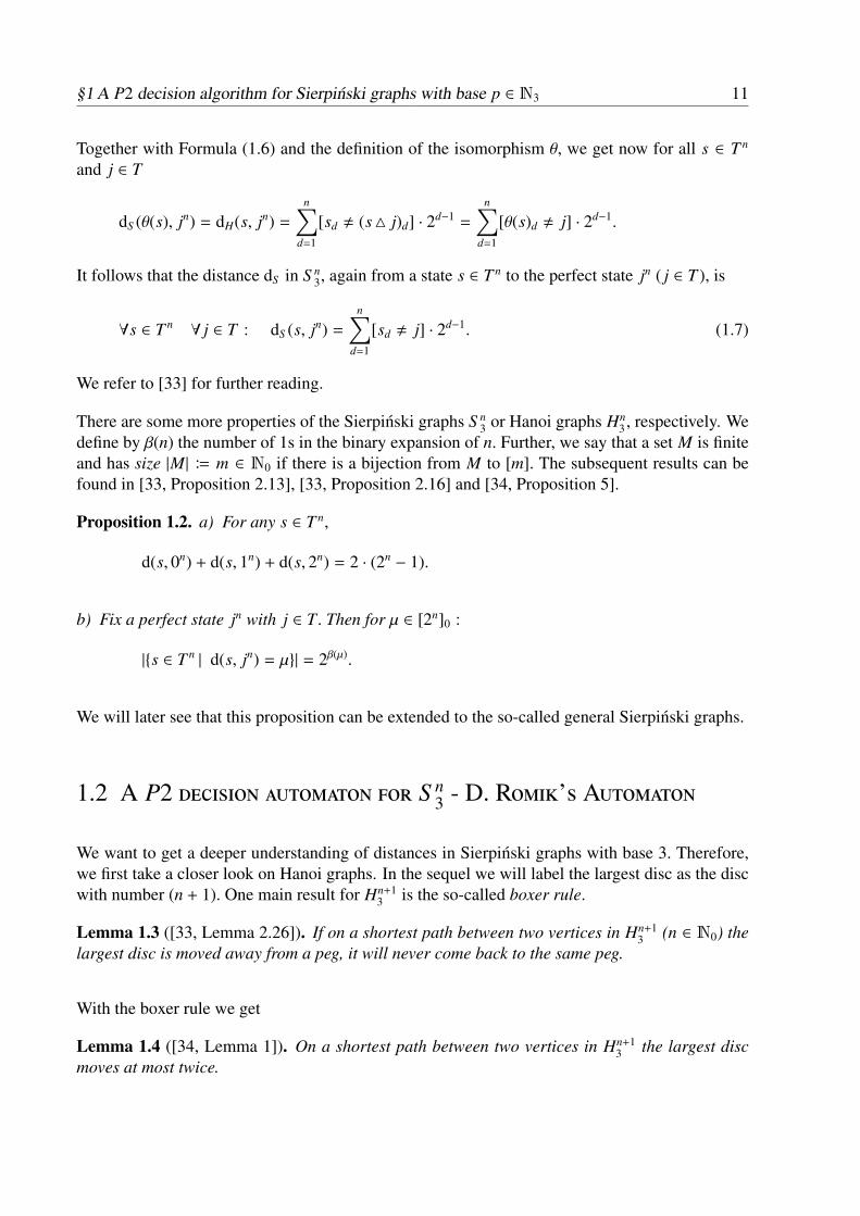
We want to get a deeper understanding of distances in Sierpinski graphs with base 3. Therefore,we first take a closer look on Hanoi graphs. In the sequel we will label the largest disc as the discwith number (n + 1). One main result for Hn+1
3 is the so-called boxer rule.
Lemma 1.3 ([33, Lemma 2.26]). If on a shortest path between two vertices in Hn+13 (n ∈ N0) the
largest disc is moved away from a peg, it will never come back to the same peg.
With the boxer rule we get
Lemma 1.4 ([34, Lemma 1]). On a shortest path between two vertices in Hn+13 the largest disc
moves at most twice.

12 §1 A P2 decision algorithm for Sierpinski graphs with base p ∈ N3
The shortest paths in Hn+13 can be categorised into three cases:
A disc (n + 1) moves only once;C disc (n + 1) moves necessarily twice;B both strategies are optimal;
as the subsequent theorem shows.
Theorem 1.5 ([34, Theorem 4], [33, Theorem 2.32]). Let s, t ∈ T n+1. Then there exist at mosttwo shortest paths between s and t. If there are two, the number of the moves of the largest discd ∈ [n + 1] for which sd , td, makes the difference. It can be one or two.
How do these two paths look like? Assume we want to go from is to jt (a P2 type problem) inHn+1
3 with s, t ∈ T n, i, j ∈ T, and i , j. (In the case that i = j, i.e., that we go from is to it, we canreduce this problem to a problem in Hn
3 , where we want to go from s to t.) Let k = 3 − i − j. If thelargest disc moves once, the path is is→ ikn → jkn → jt with length
d1(is, jt) B d(s, kn) + 1 + d(t, kn),
otherwise the path is is→ i jn → k jn → kin → jin → jt with length
d2(is, jt) B d(s, jn) + 1 + 2n − 1 + 1 + d(t, in)= d(s, jn) + 1 + 2n + d(t, in).
It is an interesting question whether for a given vertex is in Hn+13 there always exists a vertex such
that we are in case B, i.e., that both paths have equal length.
Lemma 1.6 ([33, Proposition 2.33]). For every vertex is ∈ T n+1 \ {0n+1, 1n+1, 2n+1}, n ∈ N, it canbe found a jt ∈ T n+1 (i , j) such that there are two shortest paths between these vertices in Hn+1
3 .
Remark. In [38, Corollary 3.7], it is stated that the perfect states are the only ones such that forany other regular state there is a unique shortest path with at most one move of the largest disc.
With these results we can now construct an algorithm which tells us, depending on the givenvertices, whether we are in case A,C, or B. After the evaluation of the algorithm, we know con-sequently whether we need one or two moves of the largest disc (called LDM) or both strategiesare optimal.
The underlying theorem, as well as the algorithm, is due to D. Romik [70]. At first he states thetheorem for S n
3 together with a “machine” which realises the statements of the theorem. Addition-ally, he presents a “machine” similar to the one in [33, p.145] for the isomorphism θ between Hn
3and S n
3. The two “machines” running in parallel even give us the possibility not only to determinethe number of largest disc moves but also to calculate the distance between vertices in Hn
3 . A the-orem and an algorithm which leads us directly to the decision between A,C, and B can be foundin [33, Section 2.4.3].
But we are mainly interested in the theorem for S n+13 , where we have the choice between the paths
is → i jn → jin → jt and is → ikn → kin → k jn → jkn → jt with s, t ∈ T n, i, j ∈ T, i , j, andk = 3 − i − j. If s = sd−1 . . . s1 ∈ T d−1, we define s′ = sd−2 . . . s1 ∈ T d−2 with d ∈ [n + 1]2.
§1 A P2 decision algorithm for Sierpinski graphs with base p ∈ N3 13
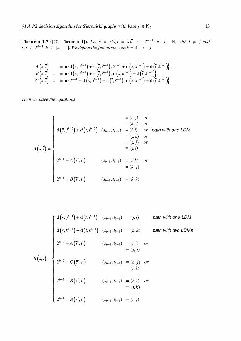
Theorem 1.7 ([70, Theorem 1]). Let s = sis, t = s jt ∈ T n+1, n ∈ N, with i , j ands, t ∈ T b−1, b ∈ [n + 1]. We define the functions with k = 3 − i − j
A(s, t
)= min
{d(s, jb−1
)+ d
(t, ib−1
), 2b−1 + d
(s, kb−1
)+ d
(t, kb−1
)},
B(s, t
)= min
{d(s, jb−1
)+ d
(t, ib−1
), d
(s, kb−1
)+ d
(t, kb−1
)},
C(s, t
)= min
{2b−1 + d
(s, jb−1
)+ d
(t, ib−1
), d
(s, kb−1
)+ d
(t, kb−1
)}.
Then we have the equations
A(s, t
)=
= (i, j) or= (k, i) or
d(s, jb−2
)+ d
(t, ib−2
)(sb−2, tb−2) = (i, i) or path with one LDM
= ( j, k) or= ( j, j) or= ( j, i)
2b−1 + A(s′, t′
)(sb−1, tb−1) = (i, k) or
= (k, j)
2b−1 + B(s′, t′
)(sb−1, tb−1) = (k, k)
B(s, t
)=
d(s, jb−1
)+ d
(t, ib−1
)(sb−1, tb−1) = ( j, i) path with one LDM
d(s, kb−1
)+ d
(t, kb−1
)(sb−1, tb−1) = (k, k) path with two LDMs
2b−2 + A(s′, t′
)(sb−1, tb−1) = (i, i) or
= ( j, j)
2b−2 + C(s′, t′
)(sb−1, tb−1) = (k, j) or
= (i, k)
2b−2 + B(s′, t′
)(sb−1, tb−1) = (k, i) or
= ( j, k)
2b−1 + B(s′, t′
)(sb−1, tb−1) = (i, j)

14 §1 A P2 decision algorithm for Sierpinski graphs with base p ∈ N3
C(s, t
)=
= (k, k) or= (k, i) or= (k, j) or
d(s, kb−1
)+ d
(t, kb−1
)(sb−1, tb−1) = (i, j) or path with two LDMs
= ( j, k) or= (i, k)
2b−1 + B(s′, t′
)(sb−1, tb−1) = ( j, i)
2b−1 + C(s′, t′
)(sb−1, tb−1) = ( j, j) or
= (i, i).
These functions stand for the three possibilities "path with one LDM", "both paths are equal",and "path with two LDMs" at the end of the reading of all pairs.
Using this theorem, we can construct a “machine” or automaton which decides between the strat-egies with one and with two LDMs (see Figure 1.3). This leads to Algorithm 1.A B C
D E(j, ·), (·, i), (i, j)(j, i) (k, k)
(k, ·),
(·, k),(i, j)
(k, k)
(i, i), (j, j)
(i, k), (k, j)
(j, i)
1
Figure 1.3: Romik’s automaton for S n3
With the algorithm we can now prove an analog to Lemma 1.6 for S n+13 .
Corollary 1.8 ([38, Corollary 3.6], [33, Proposition 4.2]). Let T = {i, j, k}. For every vertexis ∈ T n+1 \ {0n+1, 1n+1, 2n+1}, n ∈ N, it can be found a jt ∈ T n+1 (i , j) such that thereare two shortest paths between these vertices in S n+1
3 .
Proof. Every non-extreme vertex is ∈ T n+1 is of the form i1+n−dks with s ∈ T d−1 and d ∈ [n].Assuming that we go from is to jt, we want to find out which form the vertex jt must have suchthat we stay in state B of the automaton in Figure 1.3. Looking at the figure, we recognise thatfor every m ∈ T only the input (m, k4 (i4m)) leads thereto that B is not left anymore. Define thevertex jt (i , j) as jkn−d+1t with ∀δ ∈ [d − 1] : tδ = k4 (i4 sδ). Now we evaluate the pair (is, jt)

§1 A P2 decision algorithm for Sierpinski graphs with base p ∈ N3 15
Algorithm 1 The P2 decision algorithm for S n+13
procedure p2S(n, s, t)parameter n : number of discs minus 1 (n ∈ N)parameter s : initial configuration (s ∈ T n+1)parameter t : goal configuration (t ∈ T n+1, sn+1 , tn+1 )i← sn+1
j← tn+1
start in state A of the automatonδ← nwhile δ > 0 do
apply automaton to pair (sδ, tδ) . algorithm STOPs if automatonreaches state D or E
δ← δ − 1end while
end procedure
in the automaton. The first input pair (i, j) determines the automaton as in Figure 1.3. Then thefollowing n − d pairs (i, k) keep it in state A. With the pair (k, k) we move to state B. Then usingour above analysis and the definition of t we will not leave the state B anymore to the end. �
It is of interest how long the average running time of the automaton is in which it is decided, whichof the possibilities is optimal in the problem of P2 type. We will deduce this using the theory ofMarkov chains. For the basic theory we refer to [77]. We number the states A, B,C,D, and Ewith 1, 2, 3, 4, and 5. Let us consider the automaton as a Markov chain with states 1, 2, 3, 4, and 5,where we start in 1 and move from one state to another with a certain probability. The transitionmatrix P of the automaton gives these probabilities.
P =19
2 1 0 6 02 3 2 1 10 1 2 0 60 0 0 1 00 0 0 0 1
.Looking at the states 4 and 5, we see that they are a bit special in the following way. An absorbingstate is a state that, once entered, cannot be left. Then a Markov chain is called absorbing if theprocess has absorbing states. Because of the two absorbing states 4 and 5, our Markov chain isabsorbing. The matrix P is of the form
P =
(Q R0 I
).
Q is the part of the matrix which describes the transition probabilities from some transient stateto another, whereas R gives the transition probabilities from transient to absorbing states. I is the

16 §1 A P2 decision algorithm for Sierpinski graphs with base p ∈ N3
identity matrix and 0 stands for the zero matrix. In an absorbing Markov chain, Qn → 0 whenn→ ∞ and I − Q has an inverse
M = (I − Q)−1 =
∞∑n=0
Qn.
Muv is the expected number of visits which the chain made to state v provided that it has started instate u.
We get
M =
19
7 −1 0−2 6 −20 −1 7
−1
=
180133
938
9133
919
6338
919
9133
938
180133
.As we start in state 1, we get as expected time we will be in one of the states 1, 2 or 3 the sum ofthe first row
180133
+9
38+
9133
=6338.
It follows the subsequent theorem due to Romik [70]:
Theorem 1.9. The average number of disc pairs evaluated by Romik’s automaton is bounded
above by and converges, as n→ ∞, to6338.
Since in any case we also have to read the pair of largest discs (sn+1, tn+1) in addition, we calculate
altogether 1 +6338
=10138
as the number of pairs which have to be evaluated in average till thedecision problem is solved. It can also be seen that in any case at least two pairs of input data haveto be checked by the algorithm.
Remark. According to [33, pp.147], we can even reduce the number of input pairs further. Weobserve that the input of a pair with j as first component in A of the automaton in Figure 1.3will always lead to D. In this case we need only half a pair of input, and we have to check in A13·
12
+23· 1 =
56
pairs. In addition, we notice that this is also possible for C with k as firstcomponent. Using the above analysis, we accordingly need only
56·
180133
+9
38+
56·
9133
=2719
pairs of input. Together with the pair of largest discs (sn+1, tn+1), we get4619
pairs which have to bechecked in average. Still at least two pairs of input data have to be checked in any case.

§1 A P2 decision algorithm for Sierpinski graphs with base p ∈ N3 17
1.3 Sierpinski graphs S np with base p ∈ N and exponent n ∈ N0
In the last sections we have used the set T = {0, 1, 2} as the set of pegs. In the following we extendnow the set of pegs to [p]0 to define the general Sierpinski graphs with base p and exponent n.
Definition 1.10. The (general) Sierpinski graphs S np with base p ∈ N and exponent n ∈ N0 are
defined by the vertex set V(S np) = [p]n
0 and the edge set
E(S 0p) = ∅,
∀n ∈ N0 : E(S n+1p ) =
{{is, is′}
∣∣∣∣ i ∈ [p]0, {s, s′} ∈ E(S np)}
∪ {{i jn, jin} | i, j ∈ [p]0, i , j} .
(1.8)
Hence two vertices s, t ∈ [p]n0 with s = sn . . . s1 and t = tn . . . t1 are adjacent in S n
p if and only ifthere exists a d ∈ [n] such that
a) ∀k ∈ [n] \ [d] : sk = tk,
b) sd , td,
c) ∀k ∈ [d − 1] : sk = td ∧ tk = sd.
If d = 1, Condition c) is void. The same follows for Condition a) in the case d = n. This wasthe first definition of Sierpinski graphs by S. Klavžar and U. Milutinovic [52]. (Note that in [52]states are given by s1 . . . sn.)00 01 10 11
11 12 21 2210 2001 020023 3222 3321 20 30 3102 030001 101112 13
1
Figure 1.4: The Sierpinski graphs S 22 (top left), S 2
3 (bottom left), and S 24 (right)
One basic example for Sierpinski graphs is the graph S 1p for any p ∈ N, which is the complete
graph Kp on p vertices. For any n ∈ N, S n2 is isomorphic to the path P2n on 2n vertices (for S 2
2 seeFigure 1.4).

18 §1 A P2 decision algorithm for Sierpinski graphs with base p ∈ N3
Similar to (1.1) for S n3, we can define the edge set by
E(S np) =
{{si jd−1, s jid−1
} ∣∣∣∣ i, j ∈ [p]0, i , j, d ∈ [n], s ∈ [p]n−d0
}.
It is obvious that the number of vertices, namely |V(S np)|, is equal to pn. Following [68], we cal-
culate the number of edges ||S np|| = |E(S n
p)|. We see that there are exactly p extreme vertices ofdegree p − 1. The pn − p inner vertices have degree p. As a result, we get
||S np|| =
12
(p(p − 1) + (pn − p)p) =p2
(pn − 1) .
Additionally, we can observe for any n ∈ N and any p ∈ N3 that for every pair of vertices in S np
there is a path between these two vertices with the property that every vertex of S np is visited
exactly once on this path, called a Hamiltonian path.
Lemma 1.11 ([52, Proposition 3]). For any n ∈ N and any p ∈ N3 the graph S np is hamiltonian.
The graphs are connected based on Definition 1.8 or on the last lemma. Hence we can define adistance function, denoted by d, on these graphs with base p ∈ N. This was done for the first timein [52, Lemma 4] by Klavžar and Milutinovic.
Theorem 1.12 ([33, Proposition 4.5.], [52, Lemma 4]). For any j ∈ [p]0 and for any vertexs = sn . . . s1 of S n
p there is exactly one shortest path between jn and s, and
d ( jn, s) =
n∑d=1
[sd , j] · 2d−1. (1.9)
It follows that for any i, j ∈ [p]0 (i , j) the distance between the extreme vertices in and jn isd(in, jn) = 2n − 1.
Proof. We prove the theorem by induction on n. If n = 0, the statement is clearly true. Let n ∈ N0.For p = 1 it is obvious that the theorem holds. Now let p ∈ N2 and s = sn+1s, s ∈ [p]n
0. Wedistinguish two cases, namely sn+1 = j and sn+1 , j. If sn+1 = j, then we can take the shortest pathfrom jn to s in S n
p and add a j in front of each vertex. It follows that
d( jn+1, s) ≤n∑
d=1
[sd , j] · 2d−1 =
n+1∑d=1
[sd , j] · 2d−1.
If sn+1 , j, we find a path from jn+1 to s by going from jn+1 to jsnn+1 in 2n−1 steps, then moving to
sn+1 jn in one step, and finally from here to sn+1s on a (shortest) path of length ≤∑n
d=1[sd , j] ·2d−1.Hence
d( jn+1, s) ≤ (2n − 1) + 1 +∑n
d=1[sd , j] · 2d−1
≤ 2n+1 − 1 =∑n+1
d=1[sd , j] · 2d−1.
We prove now that this is the unique shortest path by obtaining that no optimal path can touch asubgraph kS n
p for sn+1 , k , j. Assume that there is a shorter path with the property that kS np is
the first subgraph which is touched by the path.
§1 A P2 decision algorithm for Sierpinski graphs with base p ∈ N3 19
Then the path contains the following parts:
• a path from jn+1 to jkn,
• the edge { jkn, k jn},
• a path from k jn to kin, j , i , k, and
• one edge in order to leave the subgraph kS np at kin.
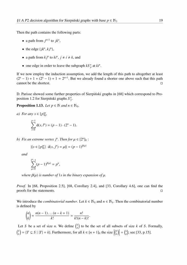
If we now employ the induction assumption, we add the length of this path to altogether at least(2n − 1) + 1 + (2n − 1) + 1 = 2n+1. But we already found a shorter one above such that this pathcannot be the shortest. �
D. Parisse showed some further properties of Sierpinski graphs in [68] which correspond to Pro-position 1.2 for Sierpinski graphs S n
3.
Proposition 1.13. Let p ∈ N and n ∈ N0.
a) For any s ∈ [p]n0,
p−1∑l=0
d(s, ln) = (p − 1) · (2n − 1).
b) Fix an extreme vertex jn. Then for µ ∈ [2n]0 :
|{s ∈ [p]n0 | d(s, jn) = µ}| = (p − 1)β(µ)
and2n−1∑µ=0
(p − 1)β(µ) = pn,
where β(µ) is number of 1s in the binary expansion of µ.
Proof. In [68, Proposition 2.5], [68, Corollary 2.4], and [33, Corollary 4.6], one can find theproofs for the statements. �
We introduce the combinatorial number. Let k ∈ N0 and n ∈ Nk. Then the combinatorial numberis defined by(
nk
)=
n(n − 1) . . . (n − k + 1)k!
=n!
k!(n − k)!.
Let S be a set of size n. We define(
Sk
)to be the set of all subsets of size k of S . Formally,(
Sk
)= {T ⊆ S | |T | = k}. Furthermore, for all k ∈ [n + 1]0 the size
∣∣∣∣(Sk
)∣∣∣∣ =(
nk
); see [33, p.15].

20 §1 A P2 decision algorithm for Sierpinski graphs with base p ∈ N3
Let G be a graph. The eccentricity of a vertex s ∈ V(G), denoted by εG(s), gives the maximaldistance between the vertex s and all the other vertices in V(G). According to [68], this integerfor a vertex s ∈ [p]n
0 in S np is given by the maximum of the distances between s and the extreme
vertices jn. The average eccentricity of G is the arithmetic mean of all eccentricities, i.e.,
ε(G) B1|G|
∑s∈V(G)
εG(s).
For n ∈ N0 and p ∈ N, the average eccentricity of S np is
ε(S np) =
1 − (2p
p − 1
)−1 2n −p − 1
p−
p−2∑k=0
(−1)p−k p − 1 − k2p − k
(pk
) (kp
)n
,
which was shown in [41]. Furthermore, we define that the diameter of G is
diam(G) := max{εG(s) | s ∈ V(G)} = max{d(s, t) | s, t ∈ V(G)}.
It was proved in [68] that for all n ∈ N and p ∈ N2 the diameter of S np is equal to 2n − 1 using the
result [52, Lemma 4]. This value 2n − 1 is especially attained by the calculation of the distancebetween the extreme vertices. Therefore, we called them extreme. In the case of Hanoi graphsHn
p, this is not true for the perfect vertices. R. Korf found out that for p = 4 and n = 15 (but notfor smaller n) the eccentricity of a perfect state and, consequently, the diameter of H15
4 is strictlylarger than the distance between two perfect states. In the calculations of the eccentricities ofperfect states in Hn
4 for n ≤ 22 in [55] and [56], it was shown that Korf’s phenomenon also occursfor n = 20 to 22.
There exists an analogue to the boxer rule in Lemma 1.3 for the S n+1p .
Lemma 1.14 ([33, Lemma 4.7]). If on a shortest path between two vertices in S n+1p (n ∈ N0) the
largest disc is moved away from a peg, it will not return to the same peg.
Proof. We prove this by contradiction. Assume that disc (n + 1) leaves iS np and returns there on a
shortest path. Then this shortest path must contain a path i jn → P′ → ikn. Since there is only oneedge between two subgraphs iS n
p and jS np, the path P′ is thereby a jin, kin-path with |{k, i, j}| = 3.
This path P′ must contain a jin, jln-path (i , l , j) such that the length of P′ is greater than orequal to 2n − 1 according to Theorem 1.12. Hence the length of the path i jn → P′ → ikn is greaterthan 2n. But by the same theorem we also know that d(i jn, ikn) < 2n. Therefore, this path cannotbe contained in a shortest path. �
In Corollary 1.8 we stated that for every non-extreme vertex of S n3 there is a vertex such that there
are two shortest paths between them.
For S np we can find a similar statement in [82].
Proposition 1.15 ([82, Corollary 3.5]). Let n ∈ N2 and p ∈ N3. Further, let s be any non-extremevertex in S n
p. Then there exists a t ∈ [p]n0 such that there are two shortest s, t-paths.

§1 A P2 decision algorithm for Sierpinski graphs with base p ∈ N3 21
As we saw, there is a correspondence of statements between the Hanoi graphs Hn3 and the general
Sierpinski graphs S np. Hinz, Klavžar, and Zemljic even showed that an isomorphic copy of S n
p isa spanning subgraph5 of Hn
p (i.e., an isomorphic embedding exists,) if and only if p is odd or ifn = 1.
Theorem 1.16 ([39, Theorem 3.1]). Let p, n ∈ N. Then S np can be embedded isomorphically
into Hnp if and only if p is odd or n = 1.
In the following theorem we characterise the distance between two arbitrary vertices more closely.Let n ∈ N0, f ∈ [p]0, and V f =
{f s | s ∈ [p]n
0
}be the set of vertices in S n+1
p consisting of all verticesbeginning with f .
Theorem 1.17 ([52, Theorem 5], [33, Theorem 4.8]). Assume p ∈ N3. Let s = sis, t = s jt ∈ [p]n+10
be two vertices with i , j, s, t ∈ [p]d0 for d ∈ [n] and s ∈ [p]n−d
0 . Then
d(s, t) = min{d(s, jd
)+ 1 + d
(t, id
),
d(s, kd
)+ 1 + 2d + d
(t, kd
)| k ∈ [p]0 \ {i, j}
}Proof. By induction on n. If n = 0, we get d = 0 and d(s, t) = 1. We note that it is sufficient toconsider only paths in the subgraph of S n+1
p whose vertices start with s. Hence we can assume thatd = n. Let n ∈ N. Let P be a shortest path among the paths between s and t which have verticesfrom Vi ∪ V j. Since P must contain the edge between Vi and V j, namely {i jn, jin}, we obtain byTheorem 1.12
|P| = d (s, jn) + 1 + d(t, in
)and the uniqueness of the so-called direct path. Now we consider a shortest path P′ between sand t with vertices only from Vi ∪ Vk ∪ V j, where k ∈ [p]0 \ {i, j} and P′ ∩ Vk , ∅. This path mustcontain the edges {ikn, kin} and {k jn, jkn} such that we get again by Theorem 1.12
|P′| = d (s, kn) + 1 + (2n − 1) + 1 + d(t, kn
).
For fixed k this so-called Vk-path is unique by the same theorem. The length of the direct pathP is obviously strictly less than 2n+1. If we consider a path which contains also vertices from asubgraph Vl with |{i, j, k, l}| = 4, its length is at least 1 + (2n − 1) + 1 + (2n − 1) + 1 = 2n+1 + 1.Hence the theorem follows. �
We know even more about shortest paths in S np.
Theorem 1.18 ([52, Theorem 6]). There are at most two shortest paths between any two verticesof S n
p.
5Let G = (V(G), E(G)) be a graph. A graph H = (V(H), E(H)) is called a subgraph of the graph G if V(H) ⊆ V(G)and E(H) ⊆ E(G). A spanning subgraph of G is a subgraph of G which contains every vertex of G.

22 §1 A P2 decision algorithm for Sierpinski graphs with base p ∈ N3
In [54], Klavžar and Zemljic introduced a new kind of vertices, called almost-extreme vertices,which are either of the form i jn or in j, where i , j. The almost-extreme vertices are obviouslythe immediate neighbours of extreme vertices. For these vertices we can calculate the distance toarbitrary vertices in S n+1
p with base p ∈ N2.
Proposition 1.19 ([54, Proposition 4]). Let m ∈ [n + 1]0, p ∈ N2, i, j ∈ [p]0, i , j, l ∈ [p]0 \ {i},and s ∈ [p]m
0 . Then
d(in−m js, inl) = d(s, im) + 2m − [ j = l] =
m∑d=1
[sd , i] · 2d−1 + 2m − [ j = l].
For the almost-extreme vertices s = i jn or in j with {i, j} ∈(
[p]02
), p ∈ N3, and n ∈ N we can also
determine the set of vertices to (or from) which two shortest paths lead. We will denote this set ofvertices by Bs.
Proposition 1.20 ([82, Theorem 3.1]). For any almost-extreme vertex s = i jn in S n+1p , we have
Bs ={t jid−1 | d ∈ [n], t ∈ ([p]0 \ {i, j})n−d+1
}.
Proposition 1.21 ([82, Theorem 3.3]). For any almost-extreme vertex s = in j in S n+1p , we have
Bs ={in−dt jd | d ∈ [n], t ∈ [p]0 \ {i, j}
}.
A class of almost-extreme vertices are the “special” vertices. We call a vertex s ∈ [p]n+10 special
with i, j, k ∈ [p]0 and |{i, j, k}| = 3, if there is a δ ∈ [n+1] such that s = sks with s ∈ ([p]\{ j, k})n+1−δ
and s ∈ [p]δ−10 .
Proposition 1.22 ([54, Proposition 7]). Let m ∈ [n], p ∈ N3, i, j, k ∈ [p]0, |{i, j, k}| = 3, ands ∈ [p]m
0 . Then
d(in−m+1s, in−m jkm) =
{d(s, km) + 2m + 1, if s is special,
d(s, jm) + 2m − [i = k](2m − 1), otherwise.
1.4 A P2 decision algorithm for Sierpinski graphs S np with base
p ∈ N3 and exponent n ∈ N0
We have seen in Section 1.2 that there exists an automaton for the Sierpinski graphs S n3 or Hanoi
graphs Hn3 , respectively, with which we can decide whether we need one LDM, two LDMs or
whether both shortest paths are of equal length. The aim of this section is to find a similar auto-maton for the Sierpinski graphs S n+1
p with base p ∈ N3 and exponent n ∈ N0. Since there is nodecision necessary for the cases p = 1 and p = 2, we omit them in the following. An alternativerepresentation of the material in this section can be largely found in the author’s article [37] withA. M. Hinz.

§1 A P2 decision algorithm for Sierpinski graphs with base p ∈ N3 23
1.4.1 The underlying principle
From the last section we already know the basic properties of the Sierpinski graphs, which wekeep in mind. In Lemma 1.14 we stated that the largest disc once removed from a peg will neverreturn there. Furthermore, we know that the diameter of S n+1
p is 2n+1 − 1 and analysed that in S n+1p
the passage through two “detour” subgraphs take at least 2n+1 + 1 moves.
We recall Theorem 1.17 about distances in S n+1p and the notation V f =
{f s | s ∈ [p]n
0
}for the set of
vertices in S n+1p consisting of all vertices beginning with f ∈ [p]0 for n ∈ N0.
Theorem 1.23 ([37, Lemma 1.1]). Let s = sis, t = s jt ∈ [p]n+10 be two vertices with i, j ∈ [p]0,
i , j, s, t ∈ [p]d0 for d ∈ [n] and s ∈ [p]n−d
0 . Then
d(s, t) = min{dk
(is, jt
)| k ∈ [p + 1]0 \ {i, j}
}.
Thereby the distance dk
(is, jt
):= d
(s, kd
)+ 1 + 2d + d
(t, kd
)for k ∈ [p]0 gives the number of
moves of the unique Vk-path realised by is → ikd → kid → k jd → jkd → jt. The distancedp
(is, jt
):= d
(s, jd
)+ 1 + d
(t, id
)is realised by the path is → i jd → jid → jt. We omitted the
prefix s which remains constant throughout the paths.
We consider the Sierpinski graphs S N+1p with N ∈ N0 in the following theorem, which is also
stated in [37] in another version. The exponent is changed to N + 1 in order to make later directuse of Formula (1.9) together with the results which arises from the application of the theorem. Ifs = sd−1 . . . s1 ∈ [p]d−1
0 , we define s′ = sd−2 . . . s1 ∈ [p]d−20 with d ∈ [N + 1]2.
Theorem 1.24. Let s = sisn−1s, t = s jtn−1t ∈ [p]N+10 , N ∈ N0, with i , j and n ∈ [N + 1],
s, t ∈ [p]n−20 , and further s ∈ [p]N+1−n
0 . If either sn−1 , i, j or tn−1 , i, j, we set the value sn−1 ortn−1, respectively, equal to h. If both are not equal to i and j and sn−1 , tn−1, we set sn−1 equal to gand tn−1 equal to h, otherwise we set both equal to h. We define the functions with k ∈ {g, h}
A′(s, t
)= min
{d(s, jn−2
)+ d
(t, in−2
), 2n−2 + d
(s, kn−2
)+ d
(t, kn−2
)}A
(s, t
)= min
{d(s, jn−2
)+ d
(t, in−2
), 2n−2 + d
(s, kn−2
)+ d
(t, kn−2
)}B
(s, t
)= min
{d(s, jn−2
)+ d
(t, in−2
), d
(s, kn−2
)+ d
(t, kn−2
)}C
(s, t
)= min
{2n−2 + d
(s, jn−2
)+ d
(t, in−2
), d
(s, kn−2
)+ d
(t, kn−2
)}.
Then we have four cases for d(s, t) depending on the pair (sn−1, tn−1)
d(s, t) =
= (i, j) or2n−1 + 1 + d
(s, jn−2
)+ d
(t, in−2
)(sn−1, tn−1) = ( j, ·) or direct path
= (·, i)
2n−1 + 1 + A′(s, t
)(sn−1, tn−1) = (g, h)
2n−1 + 1 + A(s, t
)(sn−1, tn−1) = (i, h) or
= (h, j)
2n−1 + 1 + B(s, t
)(sn−1, tn−1) = (h, h)

24 §1 A P2 decision algorithm for Sierpinski graphs with base p ∈ N3
In the second case we set k = g if only g occurs in (sn−2, tn−2), and k = h if only h occurs in thispair, and in the third and fourth case always k = h is used. Then we get
A′(s, t
)=
= (i, j) or= ( j, ·) or
d(s, jn−2
)+ d
(t, in−2
)(sn−2, tn−2) = (·, i) or direct path
= (i, l′) or= (l′, j) or= (l′,m′)
2n−2 + A′(s′, t′
)(sn−2, tn−2) = (g, h) or
= (h, g)
2n−2 + A(s′, t′
)(sn−2, tn−2) = (u′, k) or
= (k, v′)
2n−2 + B(s′, t′
)(sn−2, tn−2) = (k, k)
A(s, t
)=
= (i, j) or= ( j, ·) or
d(s, jn−2
)+ d
(t, in−2
)(sn−2, tn−2) = (·, i) or direct path
= (l, j) or= (i, l) or= (l,m)
2n−2 + A(s′, t′
)(sn−2, tn−2) = all other cases
2n−2 + B(s′, t′
)(sn−2, tn−2) = (k, k)
B(s, t
)=
d(s, jn−2
)+ d
(t, in−2
)(sn−2, tn−2) = ( j, i) direct path
d(s, kn−2
)+ d
(t, kn−2
)(sn−2, tn−2) = (k, k) Vk-path
2n−3 + A(s′, t′
)(sn−2, tn−2) = (u, i) or
= ( j, v)
2n−3 + C(s′, t′
)(sn−2, tn−2) = (k, v) or
= (u, k)
2n−3 + B(s′, t′
)(sn−2, tn−2) = (k, i) or
= ( j, k)
2n−2 + B(s′, t′
)(sn−2, tn−2) = all other cases

§1 A P2 decision algorithm for Sierpinski graphs with base p ∈ N3 25
C(s, t
)=
= (k, ·) ord(s, kn−2
)+ d
(t, kn−2
)(sn−2, tn−2) = (·, k) or Vk-path
= (u, v)
2n−2 + B(s′, t′
)(sn−2, tn−2) = ( j, i)
2n−2 + C(s′, t′
)(sn−2, tn−2) = all other cases
with u ∈ [p]0\{k, j}, u′ ∈ [p]0\{g, h, j}, v ∈ [p]0\{k, i}, v′ ∈ [p]0\{g, h, i}, l, m ∈ [p]0 \ {k, i, j}, andl′,m′ ∈ [p]0\{g, h, i, j}. These functions stand for the three possibilities "direct path", "both paths",and "Vk-path" at the end of the input of all pairs.
Proof. It is sufficient to assume s = isn−1 . . . s1 and t = jtn−1 . . . t1. If either sn−1 , i, j or tn−1 , i, j,we set the value sn−1 or tn−1, respectively, equal to h. If both are not equal to i and j and sn−1 , tn−1,we set sn−1 equal to g and tn−1 equal to h, otherwise both equal to h.According to Theorem 1.23, the length of the direct path between s and t is
d(sn−1 . . . s1, jn−1
)+ 1 + d
(tn−1 . . . t1, in−1
),
while the length of the V f -path is
d(sn−1 . . . s1, f n−1
)+ 1 + 2n−1 + d
(tn−1 . . . t1, f n−1
)for any f ∈ [p]0 \ {i, j}. We define by
∆ f B2n−1 + d(sn−1, . . . s1, f n−1
)− d
(sd−1, . . . s1, f d−1
)+ d
(tn−1, . . . t1, f n−1
)− d
(td−1, . . . t1, f d−1
)− d
(sn−1, . . . s1, jn−1
)+ d
(sd−1, . . . s1, jd−1
)− d
(tn−1, . . . t1, in−1
)+ d
(td−1, . . . t1, id−1
),
the difference between the V f -path and the direct path down to the position d ∈ [n] for anyf ∈ [p]0 \ {i, j}. We will see that there are five possibilities for ∆ f :
D ∆ f ≥ 2d direct pathA (/A′) ∆ f = 2d−1 I LDMB ∆ f = 0 I/II LDM(s)C ∆ f = −2d−1 II LDMsE ∆ f ≤ −2d V f -path,
which provides us information about the length of the path. Furthermore, it will emerge that thefinal decision between A, B, or C cannot be made until all pairs are read. To find the shortestpath(s), we distinguish several cases.

26 §1 A P2 decision algorithm for Sierpinski graphs with base p ∈ N3
1. Case: s = iisn−2 . . . s1, t = j jtn−2 . . . t1
We calculate for the length of the direct path
d(i . . . s1, jn−1
)+ 1 + d
(j . . . t1, in−1
)=
2n−1 + 1 + d(sn−2 . . . s1, jn−2
)+ d
(tn−2 . . . t1, in−2
)and for the length of the V f -path for any f ∈ [p]0 \ {i, j}
d(i . . . s1, f n−1
)+ 1 + 2n−1 + d
(j . . . t1, f n−1
)=
2n−1 + 1 + 2n−1 + d(sn−2 . . . s1, f n−2
)+ d
(tn−2 . . . t1, f n−2
).
It follows that the direct path is always the shortest as the length is at most 2n − 1. We noticethat ∆ f = 2d with d = n − 1 and we are in D.
2. Case: s = i jsn−2 . . . s1, t = jtn−1 . . . t1
The length of the direct path is at most (2n−2−1)+1+ (2n−1−1), while the V f -path is at least2n−2 + 2n−1 + 1 for any f ∈ [p]0 \ {i, j}. So the direct path is again shorter. Additionally, weremark that we are in D. The case s = isn−1 . . . s1 and t = jitn−2 . . . t1 is treated analogously.
3. Case: s = iisn−2 . . . s1, t = jhtn−2 . . . t1
Let f ∈ [p]0 \ {i, j, h}. Then the length of the V f -path is
d(i . . . s1, f n−1
)+ 1 + 2n−1 + d
(h . . . t1, f n−1
)≥ 2n + 1
and cannot be the shortest one. The possible shortest paths are the direct and the Vh-path.
3.1 Subcase: sn−2 = i, tn−2 = jIt follows that we are again in D, since ∆h = 2d with d = n − 2. Therefore, the directpath is shorter.
3.2 Subcase:
a) sn−2 = j, tn−2 = o (o ∈ [p]0 \ {h})We arrive at D with ∆h ≥ 2d (d = n − 2).
b) sn−2 = j, tn−2 = hThe length of the direct path is calculated to be
d(i j . . . s1, jn−1
)+ 1 + d
(hh . . . t1, in−1
)=
2n−1 + 1 + 2n−3 + d(sn−3 . . . s1, jn−3
)+ d
(tn−3 . . . t1, in−3
),
while the length of the Vh-path is
d(i j . . . s1, hn−1
)+ 1 + 2n−1 + d
(hh . . . t1, hn−1
)=
2n−1 + 1 + 2n−2 + 2n−3 + d(sn−3 . . . s1, hn−3
)+ d
(tn−3 . . . t1, hn−3
).

§1 A P2 decision algorithm for Sierpinski graphs with base p ∈ N3 27
Therefore, ∆h = 2d with d = n − 2, and we are in D. Then even in the worst casefor the length of the direct path, namely that all following pairs are (h, h), the directpath is the shortest as it would have only the length 2n−1 + 2n−2 + 2n−3 − 1 comparedto the length of the Vh-path 2n−1 + 2n−2 + 2n−3 + 1.
The case tn−2 = i is treated analogously.
3.3 Subcase:
a) sn−2 = i, tn−2 = hThe difference between both paths is ∆h = 2d−1 with d = n − 2, and we arrive at A.Now we look at the case A. For the cases (sn−3, tn−3) = (i, h), (h, j), (h, o), (o, h)with o ∈ [p]0 \ {h} we have ∆h = 2d−1 for d = n − 3, and we stay in A. If(sn−3, tn−3) = (h, h) we see that the direct path has length 2n−1 + 2n−2 + 2n−3 + 1 +
d(sn−4 . . . s1, jn−4
)+d
(tn−4 . . . t1, in−4
)and the Vh-path has length 2n−1 +2n−2 +2n−3 +
1 + d(sn−4 . . . s1, hn−4
)+ d
(tn−4 . . . t1, hn−4
). Hence both paths may be shortest ones
(state B) and we analyse (sn−4, tn−4) as in 3.4 a). In all other cases ∆h = 2d withd = n − 3, and we are in D.
b) sn−2 = i, tn−2 = u (u ∈ [p]0 \ {h, j})This is again D as ∆h ≥ 2d with d = n − 2.
The cases (sn−2, tn−2) = (h, j) and (v, j) with v ∈ [p]0 \ {h, i} are treated analogously.
3.4 Subcase:
a) sn−2 = h = tn−2
We are in B, since both paths have equal length. Hence we look at the next pair(sn−3, tn−3). In the cases (l,m), (i, o), (o, j), (h, i), ( j, h) with l,m ∈ [p]0 \ {h, i, j} ando ∈ [p]0 \ {h} they still have equal length, and we stay in B. For the cases (h, v) and(u, h) with u ∈ [p]0 \ {h, j} and v ∈ [p]0 \ {h, i} we see that the length of the Vh-pathis 2n−1 + 2n−2 + 2n−4 + 1 + d
(sn−4 . . . s1, hn−4
)+ d
(tn−4 . . . t1, hn−4
)and of the direct
path is 2n−1 +2n−2 +2n−3 +1+d(sn−4 . . . s1, jn−4
)+d
(tn−4 . . . t1, in−4
). So ∆h = −2d−1
with d = n − 3, and we go to C. The state C will be analysed in Case 4.3 a). Thecases (u, i) and ( j, v) (u, v as above) are treated as 3.3 a) as ∆h = 2d−1 with d = n−3.If (sn−3, tn−3) = (h, h), the Vh-path is the shorter one with ∆h = −2d (d = n − 3) andwe arrive at E (see Case 4.4). For the case ( j, i) the direct path is the shortest with∆h = 2d (d = n − 3) as we will see in Case 4.2 b) and we reach D.
b) sn−2 = o = tn−2 (o ∈ [p]0 \ {h})At this point ∆h ≥ 2d(d = n − 2) and we are in D.
3.5 Subcase:
a) sn−2 = h, tn−2 = l (l ∈ [p]0 \ {h, i, j})Here ∆h = 2d−1 with d = n − 2 and this is A as in 3.3 a). The case sn−2 = k and

28 §1 A P2 decision algorithm for Sierpinski graphs with base p ∈ N3
tn−2 = h is treated analogously.
b) sn−2 = l, tn−2 = m (l,m ∈ [p]0 \ {h, i, j} and l , m)We are again in D.
We notice that the same is true for s = ihsn−2 . . . s1 and t = j jtn−2 . . . t1.
4. Case: s = ihsn−2 . . . s1, t = jhtn−2 . . . t1
Let f ∈ [p]0 \ {i, j, h}. We must only look at the length of the direct and the Vh-path, sincethe V f -path has length at least 2n + 1 as in Case 3.
4.1 Subcase: sn−2 = i, tn−2 = jBoth paths have equal length (state B), and we can treat the subcase as in 3.4 a).
4.2 Subcase:
a) sn−2 = j, tn−2 = v (v ∈ [p]0 \ {h, i})It follows that ∆h = 2d−1 with d = n − 3. We arrive at A (see Subcase 3.3 a)).
b) sn−2 = j, tn−2 = iWe get ∆h = 2d with d = n − 2 and state D.
c) sn−2 = j, tn−2 = hBoth paths have equal length (state B). So we go back to 3.4 a).
The cases sn−2 ∈ [p]0 \ {h, j} or sn−2 = h and tn−2 = i are treated analogously.
4.3 Subcase:
a) sn−2 = i, tn−2 = hThe length of the direct path is 2n−1+1+2n−2+d
(sn−3 . . . s1, jn−3
)+d
(tn−3 . . . t1, in−3
),
while the Vh-path is 2n−1 + 1 + 2n−3 + d(sn−3 . . . s1, hn−3
)+ d
(tn−3 . . . t1, hn−3
). Thus
∆h = −2d−1 (d = n−2), and we are in C. The Vh-path seems to be the shortest. But if(sn−3, tn−3) = ( j, i), we are in state B and look at Subcase 3.4a). If we have the pairs(sn−3, tn−3) = ( j, v) and (u, i) with u ∈ [p]0 \ {h, j} and v ∈ [p]0 \ {h, i}), the Vh-pathseems again to be the shortest one, since ∆h = −2d−1 (d = n − 3), and as before wehave to analyse the next pair. If (sn−3, tn−3) = (h, ·), (·, h), (u, v) (u, v as above) theVh-path is the shortest and ∆h ≤ −2d (d = n − 3). We will show this for the case( j, h), in which the Vh-path has length 2n−1 + 2n−3 + 2n−4 + 1 + d
(sn−4 . . . s1, hn−4
)+
d(tn−4 . . . t1, hn−4
)and the direct path is 2n−1 + 2n−2 + 2n−4 + 1 + d
(sn−4 . . . s1, jn−4
)+
d(tn−4 . . . t1, in−4
)long. But even in the worst case that all subsequent pairs are ( j, i),
the Vh-path is still shorter. We reach state E.
b) sn−2 = i, tn−2 = l (l ∈ [p]0 \ {h, i, j})In this subcase ∆h = 0 (state B) and we analyse it as Case 3.4 a).

§1 A P2 decision algorithm for Sierpinski graphs with base p ∈ N3 29
The cases sn−2 = h or sn−2 = l and tn−2 = j are treated analogously.
4.4 Subcase: sn−2 = h = tn−2
Here ∆h is equal to −2d with d = n − 2, and we are in state E.
4.5 Subcase:
a) sn−2 = l, tn−2 = m (l,m ∈ [p]0 \ {h, i, j})Both paths have equal length. Thus we are in B and must analyse (sn−3, tn−3) as in3.4 a).
b) sn−2 = h, tn−2 = v (v ∈ [p]0 \ {h, i})∆h is equal to −2d−1 (d = n − 2). We are in state C and must evaluate (sn−3, tn−3) asin 4.3a).
c) sn−2 = u, tn−2 = h (u ∈ [p]0 \ {h, j})Again ∆h is equal to −2d−1 (d = n − 2), and we are in state C.
5. Case: s = igsn−2 . . . s1, t = jhtn−2 . . . t1 (g ∈ [p]0 \ {i, j, h})Let f ∈ [p]0 \ {i, j, g, h}. Then as in the previous two cases we see that the V f -path cannot bethe shortest. Therefore, we only look at the direct, the Vh- and the Vg-path.
5.1 Subcase: sn−2 = i, tn−2 = j∆h as well as ∆g is equal to 2d (d = n − 2), and we are in D.
5.2 Subcase:
a) sn−2 = j, tn−2 = o′ (o′ ∈ [p]0 \ {g, h})At this point ∆h or ∆g, respectively, is greater and equal to 2d for d = n−2 (state D).
b) sn−2 = j, tn−2 = gThe direct path has length 2n−1 + 2n−3 + 1 + d
(sn−3 . . . s1, jn−3
)+ d
(tn−3 . . . t1, in−3
)and the Vg-path 2n−1 +2n−2 +2n−3 +1+d
(sn−3 . . . s1, gn−3
)+d
(tn−3 . . . t1, gn−3
), while
the Vh−path has length ≥ 2n + 1. Hence ∆g = 2d (d = n− 2), and we go to D. In thecase with tn−2 = h we get the same only with the Vh-path instead of the Vg-path.
We can treat the cases (sn−2, i), (h, i), and (g, i) (sn−2 ∈ [p]0 \ {h, g}) analogously.
5.3 Subcase:
a) sn−2 = i, tn−2 = hThe Vg-path is longer than 2n + 1. The difference ∆h between the direct and theVh-path is 2d−1 (state A), and we proceed as in 3.3 a). The case that sn−2 = i andtn−2 = g, is treated like Subcase 3.3 a) with g instead of h as ∆g = 2d−1.
b) sn−2 = i, tn−2 = l′ (l′ ∈ [p]0 \ {g, h, i, j})The direct path is the shortest because of ∆h = 2d and ∆g = 2d for d = n − 2.

30 §1 A P2 decision algorithm for Sierpinski graphs with base p ∈ N3
The same applies to the pairs (sn−2, tn−2) = (h, j), (g, j), and (l′, j) (l′ ∈ [p]0\ {g, h, i, j}).
5.4 Subcase: sn−2 = h = tn−2
The Vg-path is once more too long. The other two are of equal length (∆h = 0 andstate B), and we look back to 3.4 a). If sn−2 = g = tn−2, the same is true with g insteadof h.
5.5 Subcase:
a) sn−2 = l′, tn−2 = m′ (l′,m′ ∈ [p]0 \ {g, h, i, j})Again the direct path is the shortest with ∆h = 2d and ∆g = 2d (d = n−2). We reachD.
b) sn−2 = h, tn−2 = v′ (v′ ∈ [p]0 \ {g, h, i})∆h is equal to 2d−1(d = n − 2), and we are in state A. The same follows for sn−2 = ginstead of h.
c) sn−2 = u′, tn−2 = h (u′ ∈ [p]0 \ {g, h, j})Again ∆h is equal to 2d−1(d = n − 2), and we are in state A. As above we cansubstitute h with g.
5.6 Subcase: sn−2 = g, tn−2 = hThe direct path is 2n−1 + 2n−2 + 1 + d
(sn−3 . . . s1, jn−3
)+ d
(tn−3 . . . t1, in−3
)long. The
Vh-path (resp. Vg-path) has the length 2n−1 + 2n−2 + 2n−3 + 1 + d(sn−3 . . . s1, hn−3
)+
d(tn−3 . . . t1, hn−3
)(with g instead of h). It follows that both ∆h and ∆g are 2d−1 for
d = n − 2. First, the direct path seems to be shorter than the other two paths, butwe have to analyse the next pair (sn−3, tn−3). We call this new state A′ because of itsspecial property and similarity to the state A. If (sn−3, tn−3) ∈ {(g, h), (h, g)} , we startanew (state A′) as before and analyse the following pair on the occurrence of g or h.Otherwise we treat this case analogously to 3.3 a) according to g or h, resp. to Vg-pathor Vh-path. We notice that the same applies to (sn−2, tn−2) = (h, g). �
Using the previous theorem, the question, whether we have to use one (LDM = 1) or two(LDM = 2) largest disc moves for an optimal solution or if both possibilities lead to an optimalpath (LDM = 0), is decided. The theorem also gives the “detour” peg k for LDM , 1. Hence wecan calculate the distance d(sis, s jt) together with Formula (1.9). We get for LDM < 2
d(is, jt) =∑n
d=1(1 − [sd = j]) · 2d−1 + 1 +∑n
d=1(1 − [td = i]) · 2d−1
= 2n+1 − 1 −∑n
d=1([sd = j] + [td = i]) · 2d−1,(1.10)
and for LDM = 2d(is, jt) =
∑nd=1(1 − [sd = k]) · 2d−1 + 2n + 1 +
∑nd=1(1 − [td = k]) · 2d−1
= 3 · 2n − 1 −∑n
d=1([sd = k] + [td = k]) · 2d−1.(1.11)
Note that for the calculation of the distance all pairs must be read, whereas for the decision only apossibly smaller number of pairs has to be read. Since we know now the shortest path(s), we canalso determine the best first move(s) to get from sis to s jt with the following lemma.

§1 A P2 decision algorithm for Sierpinski graphs with base p ∈ N3 31
Lemma 1.25 ([52, p.103], [37, Lemma 1.2]). With the same assumptions for ss := sis and j asin Theorem 1.23 the optimal first move from ss to s jid in S n+1
p is from ssb jb−1 to s jsb−1b , where
b ∈ [d + 1], s = ssd+1 . . . sb+1 ∈ [p]n−b+10 , and sb , j , i.e., b = min{δ ∈ [d + 1] | sδ , j}.
The next section makes use of the last results. We will apply them in order to construct an al-gorithm which gives us the “detour” peg k, the distance, and the best first move(s) for an arbitrarypair s and t in S N+1
p .
1.4.2 The P2 decision algorithm
We construct an algorithm, the P2 decision algorithm, which gives us the length of the shortestpath(s) between s ∈ V(S N+1
p ) and t ∈ V(S N+1p ) for p ∈ N3 and the best first move(s). Starting with
the preprocessing algorithm, we filter out the case of s = t and reduce the problem of determiningthe optimal path(s) between s = ss and t = st to find it between s and t. Then we use an algorithmto set g and h following the rules of Theorem 1.24. In Algorithm 4 we find the “detour” peg k anddecide whether we are in the case “direct path”, “both paths” or “Vk-path”. Using the results ofthe algorithms, we can go to the postprocessing algorithm, where we calculate the distance andgive the best first move(s). Note that for the case “both paths” there are two different best firstmoves.
Algorithm 2 The P2 decision algorithm for S N+1p
procedure P2S(N, p, s, t)parameter N : number of discs minus 1 {N ∈ N0}
parameter p : {p ∈ N3}
parameter s : initial configuration {s ∈ [p]N+10 }
parameter t : goal configuration {t ∈ [p]N+10 }
Pre(N, p, s, t)Post(s, t, i, j, LDM, k, n)
end procedure
We start with N + 1 discs in the P2 decision algorithm. After the preprocessing, we know n + 1,which is the maximal position, in which s and t differ. In the Detour peg algorithm, we start withδ = n. If the algorithm stops in D or in A (when the input data have run out), we set LDM equalto 1. If we end in E or C, we set LDM = 2. For the case of B as ending state we set LDM = 0. Atthe end of this algorithm, we know LDM and the “detour” peg k = � and can use this informationfor the postprocessing algorithm. The states D and A stand for the class I task (one move of thelargest disc, LDM = 1), while E and C is the class II task (two moves, LDM = 2). The class I/IItask (equality between one or two moves, LDM = 0) is represented by the state B.
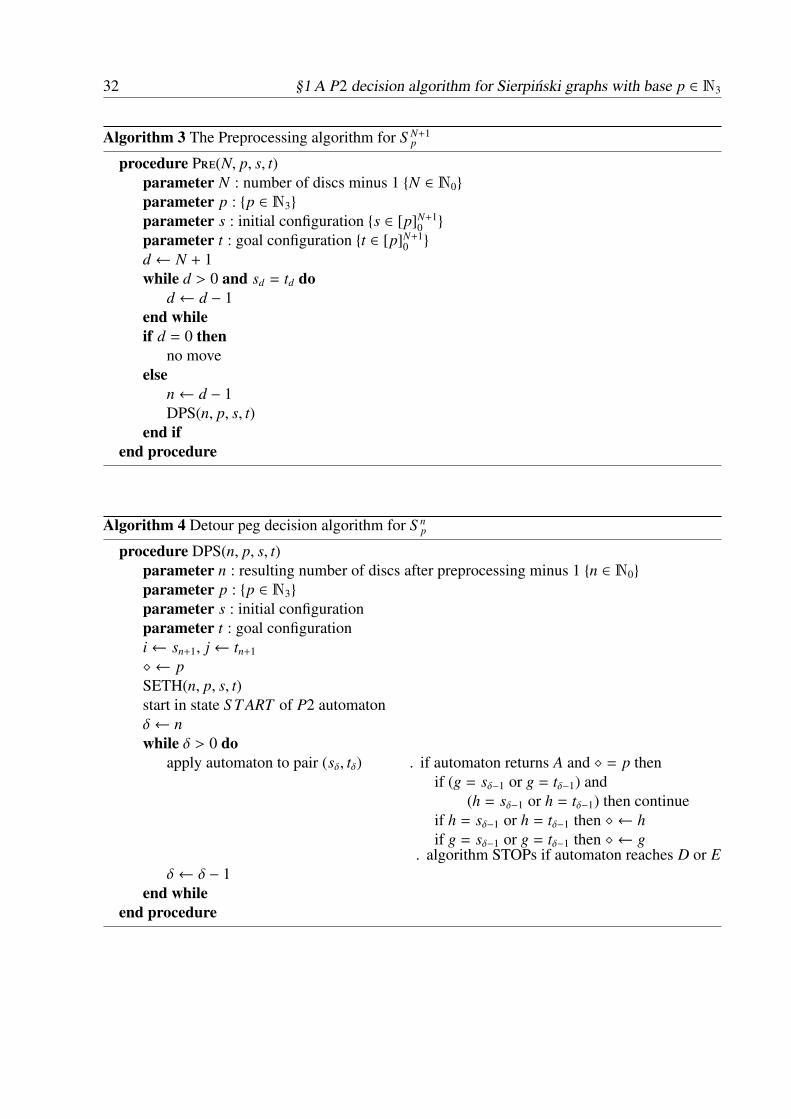
32 §1 A P2 decision algorithm for Sierpinski graphs with base p ∈ N3
Algorithm 3 The Preprocessing algorithm for S N+1p
procedure Pre(N, p, s, t)parameter N : number of discs minus 1 {N ∈ N0}
parameter p : {p ∈ N3}
parameter s : initial configuration {s ∈ [p]N+10 }
parameter t : goal configuration {t ∈ [p]N+10 }
d ← N + 1while d > 0 and sd = td do
d ← d − 1end whileif d = 0 then
no moveelse
n← d − 1DPS(n, p, s, t)
end ifend procedure
Algorithm 4 Detour peg decision algorithm for S np
procedure DPS(n, p, s, t)parameter n : resulting number of discs after preprocessing minus 1 {n ∈ N0}
parameter p : {p ∈ N3}
parameter s : initial configurationparameter t : goal configurationi← sn+1, j← tn+1
� ← pSETH(n, p, s, t)start in state S T ART of P2 automatonδ← nwhile δ > 0 do
apply automaton to pair (sδ, tδ) . if automaton returns A and � = p thenif (g = sδ−1 or g = tδ−1) and
(h = sδ−1 or h = tδ−1) then continueif h = sδ−1 or h = tδ−1 then � ← hif g = sδ−1 or g = tδ−1 then � ← g
. algorithm STOPs if automaton reaches D or Eδ← δ − 1
end whileend procedure

§1 A P2 decision algorithm for Sierpinski graphs with base p ∈ N3 33
START DI STOPI
I/II
EII STOPII
A(/A')BC
(i, j)(j, ·)(·, i)
(g, h)(i, h)(h, j)
(h, h)
(i, j)(j, ·)(·,
i)(i, l)(l, j
)(l,m)
(j, i)
(⋄, ⋄)
(⋄, ·)(·,⋄)(u, v)
(⋄, ⋄) (u, i)(j, v)
(⋄, v)(u, ⋄) (j, i)
1Figure 1.5: Automaton for the P2 decision problem with u ∈ [p]0 \ {�, j}, v ∈ [p]0 \ {�, i},
and l,m ∈ [p]0 \ {{i, j} ∪ K} , where K = {�} if � is already defined and K = {g, h}otherwise
1.4.3 Some applications
In Section 1.3 we stated some propositions about distances for vertices of a special form in S N+1p .
In the sequel we will show that several ones can be proved and extended easily with our algorithm.We recall Proposition 1.19 and even extend the statement.
Proposition 1.26 ([54, Proposition 4], [82, Theorem 3.3], [37, Proposition 2.3]). Let n ∈ [N],i, j ∈ [p]0, i , j, l ∈ [p]0 \ {i}, and s ∈ [p]n
0. Then for all problems from iNl to iN−n js (or from iN−n jsto iNl) we get LDM < 2 and LDM = 0 if and only if l , j and s = ln.
Proof. After the preprocessing, we can assume that N−n = 0. If n = 1, we end in A or D with pair(l, s1), except when s1 = l , j, in which case we stop in B. Let now n ∈ N2. If the second inputpair is (i, i) or (i, j), we go directly to D. Otherwise, i.e., for (i, sn) with sn , i, j we set sn = h = �

34 §1 A P2 decision algorithm for Sierpinski graphs with base p ∈ N3
Algorithm 5 Set g and h algorithmprocedure seth(n, p, s, t)
parameter n : resulting number of discs after preprocessing minus 1 {n ∈ N0}
parameter p : {p ∈ N3}
parameter s : initial configurationparameter t : goal configurationi← sn+1, j← tn+1
g← p, h← pif sn , i, j then
if tn , i, j and sn , tn theng← sn, h← tn
elseh← sn
� ← hend if
elseif tn , i, j then
h← tn
� ← hend if
end ifend procedure
and move to A. We move to B in the last step with (l, s1) only if sd = h = l for all d ∈ [n]. Hencewe will never end in C or E. We omit the postprocessing, since we do not want to determine thedistance exactly. �
In Proposition 1.22 we made, inter alia, a statement about distances to special vertices.
Proposition 1.27. Let n ∈ [N], i, j, k ∈ [p]0, |{i, j, k}| = 3, and s ∈ [p]n0 be special. Then
d(iN−n+1s, iN−n jkn) = d(s, kn) + 2n + 1.
Proof. After the preprocessing, the problem is reduced to determining the distance between isksand jkn with s ∈ ([p]0 \ { j, k})n−δ and s ∈ [p]δ−1
0 for a δ ∈ [n]. The second input pair can be either(i, k) or (g, k) with g ∈ [p]0 \ {k}. In the first case, we set h = k = � and go to A. Then we stayin A for the pairs (sd, k) from n − 1 to δ + 1 and move to B with (k, k) and stay there or move to Eor C for the remaining pairs. In the second case, we go to A and must then distinguish two cases.The first one has (g, k) as third input pair, such that we stay in A until we get a pair (l, k) withl ∈ [p]0 \ {g, k, j}. Then we set � = k and stay again in A until the input pair (k, k), which let usmove to B, where we again stay or move to E or C for the remaining cases. The second case hasimmediately (l, k) with l ∈ [p]0 \ {g, k, j} as input pair. Hence we proceed as above. It follows thatwe are either in LDM = 0 or LDM = 2. Hence we calculate the distance to the desired value bythe postprocessing. �

§1 A P2 decision algorithm for Sierpinski graphs with base p ∈ N3 35
Algorithm 6 The Postprocessing algorithm for S n+1p
procedure Post(s, t, i, j, LDM, k, n)parameter s : initial configuration {s ∈ [p]n+1
0 }
parameter t : goal configuration {t ∈ [p]n+10 }
parameter i : initial pegparameter j : goal pegparameter LDM : times of Largest Disc Moves {b ∈ {0, 1, 2}}parameter k : k ∈ [p + 1]0
parameter n : resulting number of discs after preprocessing minus 1{n ∈ N0}
δ← 1b← LDMif b = 0 or b = 1 then
while δ < n + 1 and sδ = j doδ← δ + 1
end whileif δ = n + 1 then
Best First Move from si jn to s jin
elseBest First Move from ssδ jδ−1 to s jsδ−1
δ
end ifdistance is d(s, t) = d(sn . . . s1, jn) + 1 + d(tn . . . t1, in)
end ifif b = 0 or b = 2 then
while δ < n + 1 and sδ = k doδ← δ + 1
end whileif δ = n + 1 then
Best First Move from sikn to skin
elseBest First Move from ssδkδ−1 to sksδ−1
δ
end ifdistance is d(s, t) = d(sn . . . s1, kn) + 1 + 2n + d(tn . . . t1, kn)
end ifend procedure
These pairs of vertices are not the only ones which can have two optimal paths. We alreadystated in Proposition 1.15 that for all non-extreme vertices there is a vertex such that there are twooptimal paths between them.
Proposition 1.28. Let p ∈ N3. For all non-extreme vertices s ∈ [p]N+10 there is a vertex t ∈ [p]N+1
0such that LDM = 0. Moreover, the vertex t can be chosen in such a way that sN+1 , tN+1, i.e., thelargest disc is N + 1.
Proof. We know that s is non-extreme. Hence it follows that there is some {i, h} ∈(
[p]02
), n ∈ [N],

36 §1 A P2 decision algorithm for Sierpinski graphs with base p ∈ N3
and s ∈ [p]n−10 such that s = iN−n+1hs. Now we choose j ∈ [p]0 \ {i, h} and set t = jhN−n+1t with,
for d ∈ [n − 1],
td = h, if sd = j,td = i, if sd = h,td = j otherwise.
Since no preprocessing is necessary, the first pair is (i, j). Then the pair (i, h) occurs N − n timessuch that we first move to A with � = h and stay there until the pair (h, h). With this pair we goto B. The remaining n − 1 input pairs are of the form ( j, h), (h, i) or (l, j) with l ∈ [p]0 \ { j, h}.Therefore, state B will not be left anymore. �
There are some other properties which can be shown with the aid of the algorithm for the generalSierpinski graphs S n
p and, consequently, also for the Hanoi graphs Hn3 . Employing the approach
of Theorem 1.24 on Sierpinski triangle graphs, we can also make a statement about distances forthis class of graphs as we will see in Section 1.5.
1.4.4 The average number of pairs to be read to solve the problem
It is of interest to us how many disc pairs must be read to solve the P2 decision problem for S N+1p .
As might be expected, this number depends on p.We already analysed this for p = 3 in Section 1.2with the aid of the theory of Markov chains. In the following section we will divide the state A ofthe automaton into A′ for the case |{i, j, g, h}| = 4 and A otherwise as in Theorem 1.24. This helpsus to distinguish easier between these two cases. We assume that s = is and t = jt with i, j ∈ [p]0,i , j, n ∈ [N], and s, t ∈ [p]n
0.In order to find the average number of pairs, we want to consider the automaton in Figure 1.5 asa Markov chain with six states in which the process starts in A′, A, or in B and move from stateto state with a certain probability. We can assume that we start in A′, A, or in B, since we knowthat the first two pairs must always be read and have therefore no direct influence on the averagenumber. The probabilities for the six states A′, A, B,C,D, and E are shown in the transition matrixof the automaton
P =1p2
2 4p − 12 2 0 p2 − 4p + 8 00 2p − 4 1 0 p2 − 2p + 3 00 2p − 4 p2 − 4p + 6 2p − 4 1 10 0 1 2p − 4 0 p2 − 2p + 30 0 0 0 p2 00 0 0 0 0 p2
.
Because of the two absorbing states in our Markov chain, this Markov chain is again absorbing.The matrix P is of the form
P =
(Q R0 I
),

§1 A P2 decision algorithm for Sierpinski graphs with base p ∈ N3 37
where Q is again the part of the matrix which describes the transition probabilities from sometransient state to another, R gives the transition probabilities from transient to absorbing states,and I is the identity matrix. In an absorbing Markov chain, Qn → 0 when n → ∞ and I − Q hasan inverse
M = (I − Q)−1 =
∞∑n=0
Qn.
Muv is the expected number of visits which the chain made to state v provided that it has started instate u.
M = (I − Q)−1 =
(p2−2)p2 −
4(p−3)p2 − 2
p2 0
0 (p2−2p+4)p2 − 1
p2 0
0 −2(p−2)
p22(2p−3)
p2 −2(p−2)
p2
0 0 − 1p2
(p2−2p+4)p2
−1
= p2
1(p2−2)
2(4p4−25p3+64p2−90p+52)(2p7−11p6+30p5−38p4−4p3+88p2−128p+64)
1(2p3−7p2+12p−8)
2(p−2)(2p5−11p4+34p3−60p2+64p−32)
0 (2p3−7p2+13p−10)(2p5−11p4+34p3−60p2+64p−32)
12(2p3−7p2+12p−8)
(p−2)(2p5−11p4+34p3−60p2+64p−32)
0 (p−2)(2p3−7p2+12p−8)
(p2−2p+4)2(2p3−7p2+12p−8)
(p−2)(2p3−7p2+12p−8)
0 (p−2)(2p5−11p4+34p3−60p2+64p−32)
12(2p3−7p2+12p−8)
(2p3−7p2+13p−10)(2p5−11p4+34p3−60p2+64p−32)
(This calculation was done with the computer algebra system Sage 5.10.) If we started in A′, weget the expected number of times we will be in A′, A, B, or C by the sum of the first row. Thesame applies to the states A, B, and C. Thus we get the (4 × 1)-vector r with the sums of the rows.Since we start at the states A′, A, and B of the automaton in Figure 1.5 with a certain probability,we must multiply the (1 × 4)-vector t of the a-priori probabilities with the vector r
t · r =(
(p−2)(p−3)p2
2p−4p2
p−2p2 0
)·
2p2(p3+p2−10p+9)(2p5−7p4+8p3+6p2−24p+16)
p2(4p−5)2(2p3−7p2+12p−8)
p2(p2+2p−4)2(2p3−7p2+12p−8)
p2(4p−5)2(2p3−7p2+12p−8)
to get the expected number of times
ANp =5p5 − 8p4 − 72p3 + 272p2 − 352p + 160
2(2p5 − 7p4 + 8p3 + 6p2 − 24p + 16)(1.12)
we will be in one of the states A′, A, B, or C depending on p.

38 §1 A P2 decision algorithm for Sierpinski graphs with base p ∈ N3
Theorem 1.29. The average number of pairs checked by the P2 decision automaton for S N+1p after
preprocessing, when the largest disc is n + 1 ∈ [N + 1] is bounded above by and converges, asn→ ∞, to 2 + ANp.
We have to add two pairs as we always have to evaluate the pairs (sn+1, tn+1) and (sn, tn) in advance.
In the cases p = 3, 4, 5, and 6 we have the values
p = 3 AN3 = 2538 ,
p = 4 AN4 = 1,
p = 5 AN5 = 68255842 ,
p = 6 AN6 = 13001037 ,
for example.
We see that for S n+13 the number 2 + AN3 = 101
38 is equal to the one we calculated in Section 1.2.
Remark. By taking a closer look on the automaton in Figure 1.5, one can reduce the number ofinput pairs further. We notice that the input of j as first component of a pair in A′ as well as in Ais always followed by a move to D. Hence we have to evaluate only half a pair in these cases. InA′ and A we just need to check p
p2 ·12 +
(p2−p)p2 · 1 =
(2p2−p)2p2 pairs, in other words, save p out of 2p2
input data. Looking at the state C, we see that this also applies to the pairs with � as first input inC. Using these results, we have to check only
ANredp =
5 p6 − 10 p5 − 69 p4 + 307 p3 − 486 p2 + 336 p − 802(2 p6 − 7 p5 + 8 p4 + 6 p3 − 24 p2 + 16 p
)pairs of input. For instance, we get for p = 3 the number ANred
3 = 67/114, for p = 4 thenumber ANred
4 = 51/56, for p = 5 the number ANred5 = 6315/5842, and for p = 6 the number
ANred6 = 7303/6222. For p = 3, 4, 5, 6 the numbers ANred
p are all strictly less than ANp.
1.5 An algorithm to determine the shortest paths in Sierpinskitriangle graphs S T n
p with base p ∈ N3 and exponent n ∈ N0
The Section 1.4.3 worked with applications of our algorithm on Sierpinski graphs themselves. Inthis section we will see that our algorithm can even be applied on another class of graphs, theSierpinski triangle graphs. These graphs have their name from the famous Sierpinski triangle (orgasket), which Wacław Sierpinski designed in 1915. He started from a closed equilateral triangleand successively removed open middle triangles such that in the step of order n ∈ N0 there aretriangular gaps of n different sizes. We can interpret the corners of the subtriangles as vertices and

§1 A P2 decision algorithm for Sierpinski graphs with base p ∈ N3 39
their sides as edges to get the class of Sierpinski triangle graphs S T n3 with base 3 and exponent n.
Since there is a connection between the Sierpinski triangle and the Sierpinski graphs (cf. [42],[33, Section 4.3]), it is not surprising that there is one between our new class of graphs and theSierpinski graphs S n
p. This relation was used by M. Jakovac in [50] to generalise the Sierpinskitriangle graphs to p ∈ N3 in the following way. Let si jδ and s jiδ with i, j ∈ [p]0, i , j, δ ∈ [n],and s ∈ [p]n−δ
0 be two vertices of the graph S n+1p . In S T n
p we identify them in one vertex, named bys{i, j}. The vertices of the form kn+1 in S n+1
p correspond to the so-called primitive vertices in S T np,
written k. Since the vertices {i, j} ∈(
[p]02
)will be important for our further study, we give them a
name, namely corner vertices. Then
Definition 1.30. The Sierpinski triangle graphs are defined by
V(S T np) =
{k∣∣∣∣ k ∈ [p]0
}∪
{s{i, j}
∣∣∣ s ∈ [p]n−δ0 , δ ∈ [n], {i, j} ∈
([p]0
2
)},
where s{i, j} stands for the contracted edge {si jδ, s jiδ} ∈ E(S n+1p ).
An explicit description of the adjacency of the vertices can be found in [50, Proposition 2.1] and[43, Definition 4]. Since S n+1
p can be built from p copies of S np, the graph S T n
p consists also ofp copies of S T n−1
p . Each pair of these copies share one vertex, in fact the corresponding cornervertex, for instance the vertex {i, j} for iS T n−1
p and jS T n−1p (i , j). There is also a recursive
definition for the class S T np similar to the one for S T n
3 ([43]). Starting from S T 0p � Kp with
V(S T 0p) = {k | k ∈ [p]0}, we take p copies of S T n
p, characterised by k ∈ [p]0, whereby we changethe labelling of all primitive vertices l except k to {k, l} and add a k to the left of all other vertices.Then the p copies are linked by identifying equal vertices.
We obtain easily that the primitive vertices have degree p−1 and all others have 2(p−1), and thatthe graphs S T n
p are connected.
Accounted for by the connection to Sierpinski graphs, there are several other consequences wecan state.
Proposition 1.31 ([43], [50, Proposition 2.3]). The graphs S T np have p
2 (pn + 1) vertices andp−1
2 · pn+1 edges.
Proof. There are two ways to prove this proposition. We will begin with the easiest way. Thevertex set V(S T n
p) contains, apart from the p primitive vertices k, exactly one half of the non-extreme vertices of S n+1
p . Hence we get
|V(S T np)| = p +
12
(|S n+1
p | − p)
= p +12
(pn+1 − p
)=
p2
(pn + 1).
A more direct way uses the fact that every vertex in S T np is of the form sn−δ . . . s1{i, j}. We have p
choices for every sk, k ∈ [n − δ], and(
p2
)choices for the pair {i, j}. Together with the p primitive
vertices, we have
|V(S T np)| = p +
n−1∑k=0
pk ·
(p2
)=
p2
(pn + 1).

40 §1 A P2 decision algorithm for Sierpinski graphs with base p ∈ N3
We determine the number of edges by:
||S T np || =
12
∑v∈S T n
p
deg(v)
=12
(p (p − 1) +
( p2
(pn + 1) − p)· 2(p − 1)
)=
p − 12
pn+1. �
A property which the Sierpinski and the Sierpinski triangle graphs have in common is the hamil-tonicity of the graphs (see Lemma 1.11).
Theorem 1.32 ([50, Theorem 3.2]). For any n ∈ N1 and p ∈ N3, the graphs S T np are hamiltonian.
We want to take a closer look at the distance dn on the graphs S T np in the next two statements.
Lemma 1.33 ([43, Proposition 1 for p = 3 and p.9]). For n ∈ N0, ν ∈ [n]0, and u,w ∈ V(S T νp)
dn(u,w) = 2n−ν dν(u,w), (1.13)
and the number of shortest paths between u and w in S T np is the same as in S T ν
p.
For the distances to the primitive vertices k we get p-independent formulas
Theorem 1.34 ([43, Theorem 1 for p = 3 and p.9]). For k, l ∈ [p]0, there is a unique shortest pathbetween k and l in S T 0
p, which has length
d0(k, l) = [k , l]. (1.14)
For ν ∈ N and u = s{i, j} with s ∈ [p]ν−10 we have
dν(u, k) = dν(s{i, j}, k) = 1 + [i , k][ j , k] +
ν−1∑d=1
[sd , k] · 2d ∈ [2ν], (1.15)
and there are 1 + [i , k][ j , k] shortest paths between u and k in S T νp.
Hence diam(S T np) = 2n (cf. [20, Proposition 1] for p = 3 and [43]) and
∀u ∈ V(S T np) :
p−1∑k=0
dn(u, k) = (p − 1) · 2n
(cf. [20, Proposition 2] for p = 3 and [43]). As in the case of Sierpinski graphs, we ask how manyoptimal paths between a vertex and a corner vertex or between two arbitrary vertices, respectively,exist. According to the recursive definition of S T n
p, we already know that dn ({l,m}, {l′,m′}) = 2n−1

§1 A P2 decision algorithm for Sierpinski graphs with base p ∈ N3 41
if {l,m}, {l′,m′} ∈(
[p]02
)and {l,m} , {l′,m′}. Together with Formulas (1.13), (1.14), and (1.15), we
have now determined the distances in S T np for n = 0 and n = 1. We will consider a path in S T n
pfrom a vertex u ∈ iS T n−1
p to a vertex w ∈ jS T n−1p as different from another u,w-path only if we
use other subgraphs kS T n−1p with i , k , j on the way from the initial vertex to the final vertex. It
will turn out that there are two possible types for shortest u,w-paths, namely the "direct type” andthe “detour type”. However, both types of paths can have equal length. We will see that in generalthere exist at most two shortest paths, except in a special case, where even three shortest paths ofequal length, one of the “direct type” and two of the “detour type”, exist.
As in the previous section, we are again interested in an algorithm to determine the shortest pathsin this new class of graphs. As Sierpinski triangle graphs with base p = 3 play sometimes a specialrole, we will start with these simpler graphs in the first subsection. In the second one we find ageneral algorithm for all p ∈ N3.
1.5.1 A P2 decision algorithm for Sierpinski triangle graphs S T n3
In this subsection we consider the Sierpinski triangle graphs S T n3 with base 3 (see Figure 1.6
for S T 33 ). From the introduction we already know that there are three primitive vertices 0, 1, and
2 of degree 2, whereas the other vertices have degree 4. With Proposition 1.31 we get
|V(S T n3 )| =
32
(3n + 1) and |E(S T n3 )| = 3n+1.
Now we want to determine the distance dn in S T n3 . For these graphs there also exists another
labelling6 which is different from the notation of Jakovac (see [43]). For a better comparison ofthe automata for S T n
3 and S T np we will maintain the previous notation. We know two statements
about the distances so far. For ν ∈ [n]0 and u,w ∈ V(S T ν3) the formula
dn(u,w) = 2n−ν dν(u,w) (1.16)
holds. Similarly, we can apply the formula for the distance between a primitive vertex and anarbitrary vertex. We recall that for k, l ∈ T
d0(k, l) = [k , l] (1.17)
and for ν ∈ N and u = s{i, j} ∈ S T ν3 with s ∈ T ν−1
dν(s{i, j}, k) = 1 + [i , k][ j , k] +
ν−1∑d=1
[sd , k] · 2d. (1.18)
Additionally, we know that dn ({l,m}, {l′,m′}) = 2n−1 if {l,m}, {l′,m′} ∈(
T2
)and {l,m} , {l′,m′}.
As explained in the introduction of this section, we have now determined the distances in S T n3 for
n = 0 and n = 1. Let n ∈ N2. We note that in S T n3 with i, c ∈ T, {l,m} ∈
(T2
), ν ∈ [n]2, and s ∈ T ν−2
dn
(is{l,m}, {c, i}
)= dn
(is{l,m}, c
)− 2n−1. (1.19)
6A labelling is a characterisation of a representative from a class of isomorphic graphs, i.e., a specific graph of thatclass.
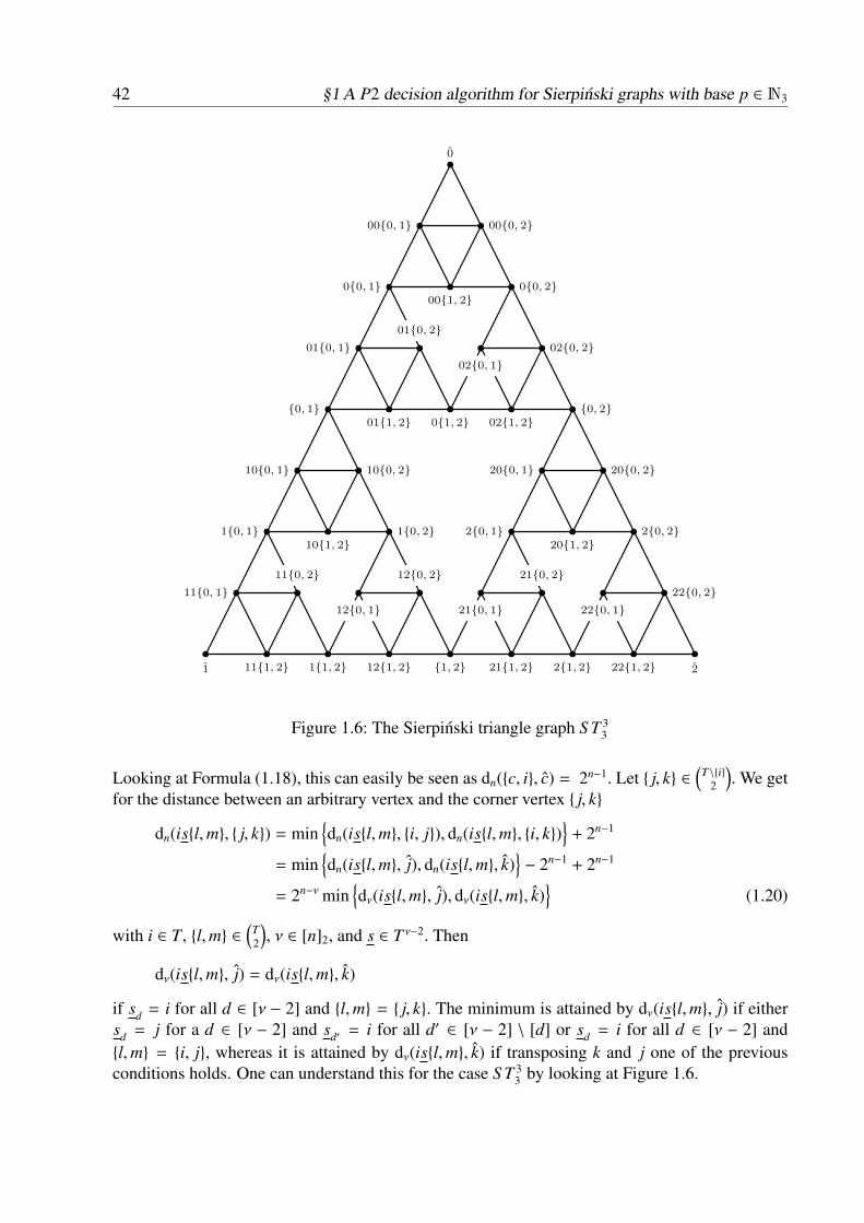
42 §1 A P2 decision algorithm for Sierpinski graphs with base p ∈ N3
1 1{1, 2} {1, 2} 22{1, 2}
0
{0, 1} {0, 2}0{1, 2}
11{1, 2} 12{1, 2} 21{1, 2} 22{1, 2}
1{0, 1} 1{0, 2}
11{0, 1}
10{1, 2}
10{0, 1} 10{0, 2}
22{0, 2}
2{0, 1} 2{0, 2}20{1, 2}
20{0, 1} 20{0, 2}
01{1, 2} 02{1, 2}
01{0, 1} 02{0, 2}
0{0, 1}00{1, 2}
0{0, 2}
00{0, 1} 00{0, 2}
11{0, 2}
12{0, 1}
12{0, 2}
21{0, 1}
21{0, 2}
22{0, 1}
01{0, 2}
02{0, 1}
1Figure 1.6: The Sierpinski triangle graph S T 3
3
Looking at Formula (1.18), this can easily be seen as dn({c, i}, c) = 2n−1. Let { j, k} ∈(
T\{i}2
). We get
for the distance between an arbitrary vertex and the corner vertex { j, k}
dn(is{l,m}, { j, k}) = min{dn(is{l,m}, {i, j}), dn(is{l,m}, {i, k})
}+ 2n−1
= min{dn(is{l,m}, j), dn(is{l,m}, k)
}− 2n−1 + 2n−1
= 2n−ν min{dν(is{l,m}, j), dν(is{l,m}, k)
}(1.20)
with i ∈ T, {l,m} ∈(
T2
), ν ∈ [n]2, and s ∈ T ν−2. Then
dν(is{l,m}, j) = dν(is{l,m}, k)
if sd = i for all d ∈ [ν − 2] and {l,m} = { j, k}. The minimum is attained by dν(is{l,m}, j) if eithersd = j for a d ∈ [ν − 2] and sd′ = i for all d′ ∈ [ν − 2] \ [d] or sd = i for all d ∈ [ν − 2] and{l,m} = {i, j}, whereas it is attained by dν(is{l,m}, k) if transposing k and j one of the previousconditions holds. One can understand this for the case S T 3
3 by looking at Figure 1.6.

§1 A P2 decision algorithm for Sierpinski graphs with base p ∈ N3 43
For the task is{l,m} → jt{l′,m′} in S T n3 with i, j ∈ T, i , j, ν ∈ [n]2, µ ∈ [ν − 1]0, s ∈ T n−µ−2,
t ∈ T ν−µ−2, and {l,m}, {l′,m′} ∈(
T2
)there are two possible types of paths, the path of direct type
and the path of detour type. For the direct type we use the iS T n−13 - and the jS T n−1
3 -subgraphsof S T n
3 . Corresponding to our understanding of difference between paths, the path of detour typemust additionally use the kS T n−1
3 -subgraph (k = 3− i− j). The paths of both types can have equallength; see for instance the task 10{1, 2} → 20{0, 2} in S T 3
3 in Figure 1.6. Hence in S T n3 there exist
at most two shortest paths.Since the S T n
3 arises by contracting the edges of S n+13 , the only vertex which two subgraphs iS T n−1
3and jS T n−1
3 (i, j ∈ T, i , j) have in common is {i, j}. Hence the direct path has length
dn
(is{l,m}, {i, j}
)+ dn
(jt{l′,m′}, {i, j}
).
Using dn({i, k}, { j, k}) = 2n−1, the detour path has length
dn
(is{l,m}, {i, k}
)+ 2n−1 + dn
(jt{l′,m′}, { j, k}
).
With Formula (1.19) we get for the direct path
dn
(is{l,m}, j
)+ dn
(jt{l′,m′}, i
)− 2n
and for the detour path
dn
(is{l,m}, k
)+ dn
(jt{l′,m′}, k
)− 2n−1.
Now we look at the difference between both paths and analyse this similarly to the case in S np
in [37]. With � ∈ {>, <,=} we deduce that
dn
(is{l,m}, j
)− dn
(is{l,m}, k
)+ dn
(jt{l′,m′}, i
)− dn
(jt{l′,m′}, k
)� 2n−1
2µ[dn−µ
(is{l,m}, j
)− dn−µ
(is{l,m}, k
)]+ 2n−ν+µ
[dν−µ
(jt{l′,m′}, i
)− dν−µ
(jt{l′,m′}, k
)]� 2n−1.
This can be summarised to
2µ[l , j][m , j] − [l , k][m , k] +
n−µ−2∑d=1
([sd , j] − [sd , k]
)· 2d
+
2n−ν+µ
[l′ , i][m′ , i] − [l′ , k][m′ , k] +
ν−µ−2∑d=1
([td , i] − [td , k]
)· 2d
� 2n−1.
If ν = n and µ = 0, we simplify this to
[l , j][m , j] − [l , k][m , k] + [l′ , i][m′ , i] − [l′ , k][m′ , k]+n−2∑d=1
([sd = k] − [sd = j] + [td = k] − [td = i]
)︸ ︷︷ ︸∈{−2,−1,0,1,2}
·2d � 2n−1.
We can follow the lines of the proofs of Proposition 1.0 and 1.2 (here no use of Proposition 1.1 isnecessary) in [37] or use the proof of Theorem 1.7 in [70] up to the last position ({l,m}, {l′,m′}).

44 §1 A P2 decision algorithm for Sierpinski graphs with base p ∈ N3AD
BE
C
({i, j}, {·, ·}), ({j, k}, {i, j}),
({j, k}, {i, k}), ({i, k}, {i, j}
({i,j}, {
i, j})
({i, k}, {j, k})
({j,k}, {
j, k}), (
{j, k}, {i
, k}),
({i,k}, {
·, ·}), ({i
, j},{j, k
})
({i, k}, {j, k})({j, k}, {i, j}),({i, j}, {i, k})
({j, k}, {j, k}),({i, k}, {i, k})({i, j}, {i, j})
1Figure 1.7: Automaton for S T n
3 in the case that ν = n and µ = 0. For ({i, k}, {i, k}) , ({ j, k}, { j, k}) inA, for ({i, j}, { j, k}) , ({i, k}, {i, j}) , ({ j, k}, {i, k}) in B and for ({ j, k}, {i, j}) , ({i, j}, {i, k}) inC, the automaton stops in the respective state.
Reaching the last position, we have to modify the automaton in Figure 1.3 or [37, Fig. 4]. Weobtain the automaton in Figure 1.7.
If ν ∈ [n]2, µ ∈ [ν − 1]0, and i , j, we can adapt the technique of the article [43] to our notation ofthe Sierpinski triangle graphs following Jakovac’s.We define
s = sn−µ−2 . . . s1{l, m}
with 3 − ((3 − l − m) M i) = l + m and (l, m) ∈(
T2
)and
t = tν−µ−2 . . . t1t0(sn−ν−1 M k) . . . (s1 M k){l′, m′}
with t0 = ((3 − l′ − m′) M j) and 3 − ((3 − l − m) M k) = l′ + m′ with (l′, m′) ∈(
T2
).

§1 A P2 decision algorithm for Sierpinski graphs with base p ∈ N3 45AD
BE
C
({i, k}, {·, ·}), ({·, ·}, {j, k}),
({j, k}, {i, k})
({i,k}, {
j, k})
({i, j}, {i, j})
({i,j}, {
·, ·}), ({·,
·}, {i, j
}),
({j,k}, {
i, k})
({i, j}, {i, j})({j, k}, {j, k}),({i, k}, {i, k})
({j, k}, {i, j}),({i, j}, {i, k})({i, k}, {j, k})
1Figure 1.8: Automaton for S T n
3 in the case that ν ∈ [n]2 and µ ∈ [ν − 1]0
Now we must only change the labels on the automaton in Figure 1.3 for the last position to get theautomaton in Figure 1.8.
1.5.2 A P2 decision algorithm for Sierpinski triangle graphs S T np with
base p ∈ N3
After we determined the shortest paths in S T n3 in the last subsection, we will now take a closer
look on S T np with p ∈ N3. We defined the Sierpinski triangle graphs S T n
p for general p inDefinition 1.30. For instance, we get for p = 4 and n = 2 the Sierpinski triangle graph S T 2
4in Figure 1.9.
In the sequel we consider two arbitrary vertices in S T np and determine the distances between them.
The cases n = 0 and n = 1 were already done in the introduction of this section, so let n ∈ N2.

46 §1 A P2 decision algorithm for Sierpinski graphs with base p ∈ N3
1 1{1, 2} {1, 2} 2{1, 2} 2
1{0, 1}1{0, 2}
1{1, 3}
1{2, 3}
2{0, 1}
2{0, 2} 2{1, 3}2{2, 3}
{0, 1}
1{0, 3}
{0, 2}
{1, 3}
2{0, 3}
{2, 3}
3{1, 2}
0{0, 1}
0{1, 2}
0{0, 2} 0{1, 3}
0{2, 3}
3{0, 1}
3{0, 2}
3{1, 3}3{2, 3}
0 0{0, 3} {0, 3} 3{0, 3} 3
1
Figure 1.9: The Sierpinski triangle graph S T 24
Let u = is{l,m},w = jt{l′,m′} ∈ V(S T np) with i, j ∈ [p]0, i , j, ν ∈ [n]2, µ ∈ [ν − 1]0, s ∈ [p]n−µ−2
0 ,
t ∈ [p]ν−µ−20 , and {l,m}, {l′,m′} ∈
([p]0
2
). Any u,w-path with only one pass through a corner vertex
must lead from u to {i, j} and then to w. Its length is
dn
(is{l,m}, {i, j}
)+ dn
(jt{l′,m′}, {i, j}
)(1.21)
= 2µ dn−µ
(is{l,m}, {i, j}
)+ 2n−ν+µ dν−µ
(jt{l′,m′}, {i, j}
)≤ 2n−1 + 2n−1 = 2n.
Another option for a u,w-path is the path through one detour subgraph, i.e., through the cornervertices {i, k} and { j, k} with k ∈ [p]0 and |{i, j, k}| = 3. Since dn({i, k}, { j, k}) = 2n−1, we see that thelength of this path is
dn
(is{l,m}, {i, k}
)+ 2n−1 + dn
(jt{l′,m′}, { j, k}
). (1.22)
Now the question arises: can a path running through more than one detour subgraph be min-imal? No, it cannot. Already in the case of two subgraphs we need more than 2n moves and,consequently, this cannot be minimal.First, we will consider the distances to corner vertices as in Formula (1.19) and (1.20) for S T n
3 .We get for any c ∈ [p]0 \ {i}
dn
(is{l,m}, {i, c}
)= dn
(is{l,m}, c
)− 2n−1.

§1 A P2 decision algorithm for Sierpinski graphs with base p ∈ N3 47
The distance between a vertex is{l,m} in S T np with i ∈ [p]0, {l,m} ∈
([p]0
2
), ν ∈ [n]2, and s ∈ [p]ν−2
0
and an arbitrary corner vertex {c, c′} ∈(
[p]0\{i}2
)can be determined as:
dn
(is{l,m}, {c, c′}
)= min
{dn
(is{l,m}, {i, c}
)+ 2n−1, dn
(is{l,m}, {i, c′}
)+ 2n−1
}= min
{2n−ν dν
(is{l,m}, c
), 2n−ν dν
(is{l,m}, c′
)}= 2n−ν min
{dν
(is{l,m}, c
), dν
(is{l,m}, c′
)}.
The path through {i, k}, c , k , c′ cannot be minimal, since we would have to go throughis{l,m} → {i, k} → {k, c} → {c, c′} and this would need more than 2n moves. The distancesdν
(is{l,m}, c
)and dν
(is{l,m}, c′
)are equal if sd , c, c′ for all d ∈ [ν − 2] and the special positions
are either {l,m} = {c, c′} or {l,m} = {l′,m′} with {l′,m′} ∈(
[p]0\{c,c′}2
); as for instance the task 1{1, 2}
to {0, 3} in S T 24 in Figure 1.9. The minimum is attained by the first distance if either sd = c for a
d ∈ [ν − 2] and sd′ , c, c′ for all d′ ∈ [ν − 2] \ [d] or sd , c, c′ for all d ∈ [ν − 2] and {l,m} = {l′, c}with l′ ∈ [p]0 \ {c′}, whereas it is attained by the second one if transposing c and c′ one of theprevious conditions holds.
In the following we look at the distance between two arbitrary vertices in S T np. For ν ∈ [n]2,
µ ∈ [ν− 1]0, i, j ∈ [p]0, and i , j, let u = isn−µ−2 . . . s1{l,m} and w = jtν−µ−2 . . . t1{l′,m′} be verticesof S T n
p with {l,m}, {l′,m′} ∈(
[p]02
). As in the last subsection, we analyse the length difference
between the two types of paths similarly to the case of S np in [37]. We already determined the
distances in Formulas (1.21) and (1.22). For the difference between the distances of both possibletypes of paths between u and w we get with � ∈ {>, <,=} :
[l , j][m , j] − [l , k][m , k] +
n−ν−1∑d=1
([sd = k] − [sd = j]) · 2d+([sn−ν = k] − [sn−ν = j] + [l′ , i][m′ , i] − [l′ , k][m′ , k]
)· 2n−ν+
n−µ−2∑d=n−ν+1
([sd = k] − [sd = j] + [tν−n+d = k] − [tν−n+d = i]) · 2d � 2n−1.
With g := sn−µ−2 and h := tν−µ−2 we can deduce that
[l , j][m , j] − [l , k][m , k] +
n−ν−1∑d=1
([sd = k] − [sd = j]) · 2d+([sn−ν = k] − [sn−ν = j] + [l′ , i][m′ , i] − [l′ , k][m′ , k]
)· 2n−ν+
n−µ−3∑d=n−ν+1
([sd = k] − [sd = j] + [tν−n+d = k] − [tν−n+d = i]) · 2d
� 2n−µ−2 ·(2µ+1 − ([g = k] − [g = j] + [h = k] − [h = i])
).
We proceed on the same lines as in [37] with respect to the special positions {l,m} and {l′,m′}. Ifν < n, we can stop after the reading of (sn−ν, {l′,m′}) except in the case where we are in B. Then

48 §1 A P2 decision algorithm for Sierpinski graphs with base p ∈ N3
we define for d ∈ [n − ν − 1]
td = i, if sd = j;= k, if sd = k;= j, if sd = x, x ∈ [p]0 \ {k, j};
and˜t = i, if {l,m} = { j, u}, u ∈ [p]0 \ {k};
= k, if {l,m} = {k,w}, w ∈ [p]0 \ { j};= j, in all other cases.
These pairs will be evaluated in a special automaton, namely Automaton 3.
We update the old Automata 0, 1, and 2 of [37] with the new types of pairs and get the new threeAutomata 0,1, and 2.
The four Automata 0, 1, 2, and 3 in Figures 1.11, 1.12, 1.13, and 1.10 together can be used inthe same way as in [37] to determine the distances between arbitrary vertices in S T n
p. Apply-ing our automata, we can carry Algorithm 1 in [37] over to the Sierpinski triangle graphs S T n
pwith base p ∈ N3, where we have to keep in mind that we can stop the evaluation with the pair(sn−ν, {l′,m′}) except in the case where we are in B and have to apply Automaton 3 in addition.According to our understanding of difference between paths, we see that there are at most twodifferent shortest paths between arbitrary vertices with the exception of the following cases. Fori, j, g, h ∈ [p]0 and |{i, j, g, h}| = 4 we consider the tasks from isδ{g, h} to jtδ{g, h} with δ ∈ [n−1]0
and (sd, td) ∈ {(g, h), (h, g)} for all d ∈ [δ] and from i{l,m} to j{l,m} with {l,m} ∈(
[p]0\{ j,i}2
)in S T n
p.Note that for these cases p must be in N4. Using Algorithm 1 in [37] together with our automata,we see that we end in state B for both tasks, but with two possible ks, namely k = g or h for thefirst case and k = l or m in the second one. Hence we have altogether three shortest paths, one ofthe direct type and two of the detour type; see for instance from 1{0, 3} to 2{0, 3} in the graph S T 2
4in Figure 1.9.
BD E(j
, i),({j, u}, i)
(k, k), ({w, k}, k)
(·, j)
1
Figure 1.10: Automaton 3

§1 A P2 decision algorithm for Sierpinski graphs with base p ∈ N3 49
1A 0 B
D(i, k),(k, j),
({w, k}, {i, k}),({j, k}, {v, k}),({x, x′}, {v, k}),({w, k}, {y, y′}),(k, {i, k}),(k, {y, y′}),(x, {v, k})
| {g, h, i, j} |= 4
(i, j),(j, ·),(·, i),all other pairs ({·, ·}, {·, ·}),(x, {i, k}),(·, {i, u}),(j, {·, ·})(k , k), ({w , k}, {v , k}), (k , {v , k})
1Figure 1.11: Automaton 0 with u ∈ [p]0 \ {k}, v ∈ [p]0 \ {i},w ∈ [p]0 \ { j}, x, x′ ∈ [p]0 \ {k, j}, and
y, y′ ∈ [p]0 \ {k, i}, where x , x′ and y , y′
1.6 Conclusion and Outlook
In this chapter we proved a theorem which determines all shortest paths between two arbitraryvertices sis and s jt in the Sierpinski graphs S N+1
p with base p ∈ N3 and exponent N + 1 ∈ N1.We gave a P2 decision algorithm with four included algorithms and an automaton which we needin order to determine the distance and the best first move(s). In this decision algorithm we firstfilter out the cases where the vertices are equal and omit s, fix the values of the second input pairin the next step, then run through an automaton in order to find the index of the possible “detour”subgraph, and determine in the last algorithm the best first move(s) and calculate the distance. Weapplied our results on already known metric properties of Sierpinski graphs in order to simplifytheir proofs. Moreover, we calculated the average number of pairs which have to be read to get adecision.

50 §1 A P2 decision algorithm for Sierpinski graphs with base p ∈ N3
A 1 BD
(b, k), (k, a),({w, k}, {i, k}), ({b, k}, {a, a′}),({j, k}, {v, k}), ({b, b′}, {a, k}),(k, {i, k}), (b, {a, k}), (k, {a, a′})
(j, ·), (·, i), (b, a),({j, k}, {i, k}), ({b, b′}, {a, a′}),({g, c}, {i, h}), ({h, c′}, {i, g}),({j, u}, {·, ·}), ({j, k}, α),({·, ·}, {i, u}), ({b, b′}, α),({g, h}, {i, a}), ({j, b}, {g, h}),(j, {·, ·}), (·, {i, a}), (u, {i, k}), (b, {a, a′}),(g, {h, i}), (h, {g, i})
(k, k), ({w, k}, {v, k}),({g, h}, {g, h}), (k, {v, k})
1
Figure 1.12: Automaton 1 with u ∈ [p]0 \ {k}, v ∈ [p]0 \ {i},w ∈ [p]0 \ { j}, c ∈ [p]0 \ {h},c′ ∈ [p]0 \ {g}, a, a′ ∈ [p]0 \ {i, g, h}, and b, b′ ∈ [p]0 \ { j, g, h}, where a , a′
and b , b′. For the input {·, ·} we choose α ∈(
[p]02
)\ {{v, k}, {g, h}} . Note that we
stay in state 1 for the pairs (g, h), (h, g), ({b, b′}, {g, h}), ({g, h}, {a, a′}), ({b, h}, {a, g}),({b, g}, {a, h}), (g, {h, a}), (h, {g, a}), and (b, {g, h}).
Romik provided in his paper [70] in addition to his decision automaton for S n3 an automaton
(cf. [70, Fig. 3.2]) which computes the distance for arbitrary vertices in S n3 directly by running
through the automaton. This could be a development of the here stated automaton for the gen-eral S N+1
p by adding additional counters for the distance and the variable N. Our algorithm canbe useful in the further study of the metric structure of the Hanoi graphs, since according to The-orem 1.16 S N+1
p is embedded as a spanning subgraph into HN+1p for odd p or for N = 1. At the
moment the Hanoi graph H154 is analysed concerning its diameter diam(H15
4 ) on the SuperMUCwhich is the high-end supercomputer at the Leibniz-Rechenzentrum (Leibniz SupercomputingCentre) in Garching near Munich. The project is named HLRB Project pr87mo ([44]).In the last subsection we modified the P2 decision algorithm for Sierpinski triangle graphs. We de-termined for the first time all shortest paths in this new class of graphs. One interesting use of thiscould be the further analysis of the Sierpinski triangle graphs concerning their metric propertieslike the eccentricity and the average eccentricity.

§1 A P2 decision algorithm for Sierpinski graphs with base p ∈ N3 51AD
BE
C
(j, ·), (·, i), (x, y),
({i, j}, {v, k}), ({j, ·}, {y, y ′}), ({j, ·}, {i, ·}),
({w, k}, {i, u}), ({x, x ′}, {i, u}), ({u, u ′}, {i, k})
({u, ·}, {y, y ′}), (j, {·, ·}), (w, {i, u}), (x, {i, k}), (x, {·, u})
(j,i),
({j,u}, {
i, u}), (
j, {i, u})
(k, k), ({w, k}, {v, k}), (k, {v, k})
(k,·), (·
, k), (x
, y),
({w,k}, {
k, ·}), (
{j, k}, {v
, ·}),({w,
k}, {·, ·})
,
({k,·}, {
y, y′ }), (
{·, ·}, {v,
k}),({k,
·}, {i, k
}),
(k,{·, ·}
), (x, {k
, ·}),(j,
{v, k})
(k, k), ({w, k}, {v, k}),(k, {v, k})
(x, i), (j, y),({j, u}, {i, k}), ({j, u}, {y, y′}),({j, k}, {i, u}), ({x, x′}, {i, u}),(j, {i, k}), (j, {y, y′}), (x, {i, u})
(x, k), (k, y),({w, k}, {i, k}), ({j, k}, {v, k}),({w, k}, {y, y′}), ({x, x′}, {v, k}),(k, {i, k}), (x, {v, k}), (k, {y, y′})
(j, i), ({j, u}, {i, u}), (j, {i, u})
1Figure 1.13: Automaton 2 with u, u′, u ∈ [p]0 \ {k}, v ∈ [p]0 \ {i}, w ∈ [p]0 \ { j}, x, x′ ∈ [p]0 \ {k, j},and y, y′ ∈ [p]0 \ {k, i}, where x , x′, y , y′, and u , u′.


Chapter 2
Variations on the Tower of Hanoi with 3 pegs
There are many variations known on the classical Tower of Hanoi with three pegs. One can modifythe colours of the discs and the rules for the moves (see [33, Chapter 6] for further reading) or justrestrict the allowed moves regarding their orientations. The new versions with excluded movescan be described by digraphs D = (V(D), A(D)) whose vertices v ∈ V(D) are the pegs and whosearcs (i, j) ∈ A(D) mean that a disc may move from peg i to peg j. The variant of the Tower ofHanoi where the oriented disc moves are defined by the digraph D will be named T H(D).
Remark. In several articles these digraphs D are called Hanoi graphs; see for instance [10], [58],and [57]. But we will use the term Hanoi graph as defined in the book [33].
A T H(D) is solvable if for any choice of source and goal peg and for every number of discs thereexists a sequence of legal moves to transfer the tower of discs from the source peg to the goal peg.
We know from [33, Theorem 8.4] that for every digraph D = (V(D), A(D)) with at least threevertices the T H(D) is solvable if and only if D is strongly connected, i.e., if for any pair of distinctvertices v,w ∈ V(D) there exists a directed path from v to w and a directed path from w to v. Forthree pegs we have five strongly connected digraphs which are not isomorphic (see [74]). Thesedigraphs are depicted in Figure 2.1.
In the upper row of Figure 2.1 we see from left to right the digraph C3 of the Cyclic TH, L3 of theLinear TH, and C+
3 of the T H(C+3 ). Underneath them we have the digraph K−3 of the T H(K−3 ) and
the (di)graph K3 of the well-known T H(K3), whose state graph is the classical Hanoi graph Hn3 .
The state graphs of the other variants arise from the Hn3 by transforming the Hn
3 into directedgraphs considering the allowed moves between the pegs in the different cases. In Figure 2.2 thedirected graphs for T H(C+
3 ) and T H(K−3 ) are shown.
In the sequel we focus on problems of P0 type (i.e., to go from a perfect state to a perfect state)on the above-mentioned towers and the minimal number of moves for their solution. For solvingthe problems there exists one algorithm for all these variants which is due to A. Sapir [74]. Forsome variants there already existed algorithms before. For the classical T H(K3) an algorithm was
53

54 §2 Variations on the Tower of Hanoi with 3 pegs
b b
b
0 12 C3
a
bc
b b b0 1 2
L3
a
a
b
b
b b
b
0 12C+
3
a
a
bc
b b
b
0 12K−
3
a
a
bb
c
b b
b
0 12 K3
a
a
bb
cc
1
Figure 2.1: The strongly connected digraphs on three vertices
111 112110120122 121102 100101 211212 210220222221202200 201
011012010020022021 002000001
111 112110120122 121102 100101 211212 210220222221202200 201
011012010020022021 002000001
1
Figure 2.2: The directed state graphs of T H(C+3 ) and T H(K−3 ) for n = 3
given by Lucas’s nephew Raoul Olive. Hence this algorithm is named Olive’s algorithm in theliterature (see [33, pp. 74–75]). The Linear TH (or three-in-a-row Hanoi) appeared first in 1944 in[75, p. 99]. H. Hering took then a closer look at this variant in [32]. An algorithm for the optimalsolution can be found in [33, pp. 242–244]). In 1981, M. D. Atkinson described the Cyclic THand also presented an algorithm for its solution in [9]. With Algorithm 7 all these variants can beuniquely solved with a minimum number of moves, as stated in the following theorem.

§2 Variations on the Tower of Hanoi with 3 pegs 55
Algorithm 7 The Sapir Algorithmprocedure SAP(D, n, i, j)
parameter D : strongly connected digraph with V(D) = Tparameter n : number of discs {n ∈ N0}
parameter i : source peg {i ∈ T }parameter j : goal peg { j ∈ T }if n ≥ 1 and i , j then
k ← 3 − i − jif there is an arc from i to j then
S AP(D, n − 1, i, k)move disc n from i to jS AP(D, n − 1, k, j)
elseS AP(D, n − 1, i, j)move disc n from i to kS AP(D, n − 1, j, i)move disc n from k to jS AP(D, n − 1, i, j)
end ifend if
end procedure
Theorem 2.1. For every strongly connected digraph D with three vertices / pegs the T H(D) canbe uniquely solved by Algorithm 7 with the minimum number of moves.
Proof. A proof of this theorem can be found in [33, p. 245f] or [74, Theorem 1] or for theCyclic TH in [9]. �
The Sapir Algorithm 7 gives rise to an infinite sequence of moves for each T H(D), with D as inFigure 2.1, which is obtained as the limit of the finite sequences of moves for n discs as n goesto infinity. More details on these sequences will be given in the later sections. The sequences aredefined on the basic alphabet {a, b, c, a, b, c} excluding the forbidden moves in each special case.We illustrate the labelling in Figure 2.1. Now our special interest lies in the sequences for T H(K−3 )and T H(C+
3 ). From J.-P. Allouche [7] we know that both are morphic sequences. We want toinvestigate whether they are automatic.For the other three variants this is already known. Allouche and F. Dress showed in [5] that theT H(K3) sequence is 2-automatic. Additionally, they gave an automaton with which we can findthe n-th move in T H(K3) with n as binary number (evaluating from right to left and n ∈ N).Allouche and Sapir [7] proved using Algorithm 7 that the Linear TH sequence is 3-automatic. Incontrast, the Cyclic TH sequence is not d-automatic for any d, as it was shown in [2] by Allouche.In [7], Allouche and Sapir conjectured that the only Hanoi sequences with restricted moves whichare d-automatic for some d are the T H(K3) sequence and the Linear TH sequence. This wasformulated as a conjecture in [33, Chapter 9] (cf. Chapter 0).

56 §2 Variations on the Tower of Hanoi with 3 pegs
2.1 Words, morphisms, and sequences
We will outline the most important definitions and theorems for our further considerations, espe-cially concerning morphic and automatic sequences. For the statements concerning matrix ana-lysis one may look into some standard source for the theory, as for instance [48].
Let Σ be a finite set of letters. We call Σ an alphabet. Further, let n ∈ N0. Then a finite word s isa map from [n]0 to Σ and is written as s = s0s1 . . . sn−1. In the case of n = 0 the word is the emptyword, denoted by ε. The set Σ∗ is the set of finite words on Σ.
Example 2.2. Let Σ = {0, 1}. Then Σ∗ = {ε, 0, 1, 00, 01, 11, 10, 000, 001, . . .}.
If s ∈ Σ∗, then its length |s| is the value n of the corresponding map between [n]0 and Σ, i.e., thenumber of letters in s. Note that |ε | = 0. Assume the letter a is an element of Σ, then the numberof its occurrences in s is denoted by |s|a. The set Σ is a subset of Σ∗ in the sense that a letter a ∈ Σ
can be identified with a word of length 1.
Let s, t ∈ Σ∗. The operation st is the concatenation of s and t which is the consecutive writing ofthe words s and t. In general, the concatenation is not commutative, whereas it is associative asr(st) = (rs)t for all finite words r, s, and t. This operation together with the set Σ∗ is a monoid7,where the empty word is the identity element.We say that s′ , ε is a prefix of s if there exists an s′′ ∈ Σ∗ such that s = s′s′′. The word s′ , ε is astrict prefix of s if s′′ , ε. We say that a word s is a subword or (factor) of a word w if there existwords r and t such that w = rst.Similarly to the definition of a finite word, an infinite word can be viewed as a map from N0 to Σ.In our text we will use the term sequence for an infinite word. Let s = s0s1s2 . . . be a sequence.For i ∈ N0 we set s[i] = si and for i ∈ N0 and j ≥ i we define s[i... j] = sisi+1 . . . s j.
Example 2.3. As an example we give the Prouhet-Thue-Morse sequence
t = 0110100110010110 . . . .
The i-th element t[i] = ti of t is equal to 0, if the number of 1s in the binary expansion of i is even,and equal to 1, if it is odd; see for instance [1].
A basic tool in working with alphabets and words is the morphism (or homomorphism). Let ∆ beanother alphabet. A morphism is a map ψ : Σ∗ → ∆∗ which satisfies ψ(st) = ψ(s)ψ(t) for allwords s, t ∈ Σ∗. If Σ = ∆, we call the map an endomorphism and can iterate the application of ψ.Then ψ0(a) = a and ψn(a) = ψ(ψn−1(a)) for all a ∈ Σ and n ∈ N.
Morphisms can have several properties. A morphism ψ : Σ∗ → ∆∗ is k-uniform for k ∈ N if|ψ(a)| = k for all a ∈ Σ. A 1-uniform morphism is a coding.
7A monoid S is a set that is closed under an associative binary operation and has an identity element i ∈ S such that,for all a ∈ S , ia = a = ai; see for instance [49].

§2 Variations on the Tower of Hanoi with 3 pegs 57
Example 2.4. The Prouhet-Thue-Morse sequence t of Example 2.3 is generated by the 2-uniformmorphism ψ : {0, 1}∗ → {0, 1}∗ which is given by
0 → 01,1 → 10.
For a proof we refer to [1, Proposition 3].
If ψ(a) , ε for all a ∈ Σ, then ψ is non-erasing. If ψ(a) = ε for all a ∈ Σ, then we say that ψ istrivial.
One very important type of morphisms is the primitive endomorphism because of its special prop-erty. An endomorphism ψ : Σ∗ → Σ∗ is primitive if there exists an n ∈ N such that for alla, b ∈ Σ the letter a occurs in ψn(b). The name is connected with the primitivity of the so-calledincidence matrix of ψ.Let Σ = {a1, a2, . . . am}, ∆ = {b1, b2, . . . bn}, and ψ : Σ∗ → ∆∗. The incidence matrix (or transitionmatrix or substitution matrix) M(ψ) of the morphism ψ is
M(ψ) = (mi, j) i∈[n]j∈[m]
where mi, j = |ψ(a j)|bi , i.e., mi, j is the number of occurrences of bi in ψ(a j). For n = m we definethat M0 = I and for all k ∈ N : Mk+1 = Mk · M. An (n × n)-matrix M = (mi, j)i, j∈[n] is non-negative,denoted by M ≥ 0, if mi, j ≥ 0 for every i, j ∈ [n], and is positive, written M > 0, if mi, j > 0 forevery i, j ∈ [n]. A non-negative matrix M is primitive if there exists a k ∈ N such that all entriesof Mk are positive. We see that an endomorphism is primitive if and only if its incidence matrix isprimitive.
A non-negative matrix is reducible if there exists a permutation matrix8 P such that
P−1MP =
(A1 R0 A2
)or M = P
(A1 R0 A2
)P−1 (2.1)
where A1, A2 are square matrices, and 0,R are rectangular matrices such that the dimensionsmatch. If a non-negative matrix is not reducible, we say that it is irreducible.
Lemma 2.5. Every primitive matrix is irreducible.
Proof. This statement is a direct consequence of [8, Proposition 8.3.4 (e)], which says: LetM = (mi, j)i, j∈[n] be a non-negative (n × n)-matrix. The matrix M is irreducible if and only if foreach i, j there exists a k = k(i, j) such that mk
i, j is positive (and there is such a k with k ∈ [n]). �
Lemma 2.6 ([48, Theorem 8.5.6]). Let P be a primitive (n × n)-matrix. Then there exists ans ≤ (n − 1) nn such that Ps > 0.
8Let n ∈ N. An (n × n)-matrix P is a permutation matrix if exactly one entry in each row and column is equal to 1and all other entries are 0.

58 §2 Variations on the Tower of Hanoi with 3 pegs
In order to explain what morphic and automatic sequences are, we return to endomorphisms. Letψ : Σ∗ → Σ∗ be an endomorphism. If there exist a letter a ∈ Σ and a word s ∈ Σ∗ such thatψ(a) = as and ψn(s) , ε for each n ∈ N, we say that the endomorphism ψ is prolongable on a ∈ Σ.Then we see that ψn+1(a) = ψn(ψ(a)) = ψn(as) = ψn(a)ψn(s), and as a consequence that ψn(a) isa strict prefix of ψn+1(a) for all n ∈ N. Hence limn→∞ ψ
n(a) exists and is infinite. This limit isdenoted by
ψ∞(a) := limn→∞
ψn(a) = asψ(s)ψ2(s)ψ3(s) . . .
which is a fixed point of (the extension by continuity of) the endomorphism ψ (to infinite se-quences), i.e., ψ(ψ∞(a)) = ψ∞(a). Often we will refer to such a sequence as an (iterative) fixedpoint of a morphism.
Definition 2.7. If a sequence s is an iterative fixed point of an endomorphism ψ, more preciselys = ψ∞(a), it is pure morphic. If there exists a coding τ : Σ∗ → ∆∗ and s = τ(ψ∞(a)), we call thesequence morphic.
Example 2.8. Recall Examples 2.3 and 2.4. Then t = ψ∞(0) (cf. [1, Proposition 3]).
Example 2.9. Recall the Cyclic TH sequence mentioned above. Its alphabet is {a, b, c}. Thissequence is the image, under the coding τ : { f , g, h, u, v,w}∗ → {a, b, c}∗, of the fixed point of theendomorphism ψ on { f , g, h, u, v,w}∗ where
τ( f ) = a = τ(w), τ(g) = b = τ(u), τ(h) = c = τ(v),
and
ψ( f ) = f v f , ψ(g) = gwg,ψ(h) = huh, ψ(u) = f g,ψ(v) = gh, ψ(w) = h f .
The proof can be found in [5, Section 5] and [7, Theorem 1]. Obviously, it is a morphic sequence.
We keep in mind that a (pure) morphic sequence can be an iterative fixed point of two differentmorphisms which are not powers of the same morphism.
The following type of endomorphisms plays an important role in our investigation.
Definition 2.10. Let d ∈ N2. A sequence s is d-automatic if it is the image, under a coding, of aniterative fixed point of a d-uniform morphism.
Example 2.11. As examples we will take a closer look on the T H(K3) sequence, or (classical)Hanoi sequence, and the Linear TH sequence. The first one is defined on the basic alphabet{a, b, c, a, b, c}. Its prefixes of length 2N − 1 give the minimal sequence of moves in the classicalHanoi game to transfer N discs from peg 0 to peg 1 if N is odd and from peg 0 to peg 2 if Nis even. The sequence is the iterative fixed point of the 2-uniform morphism, given on the basicalphabet by
a→ ac, a→ ac,b→ cb, b→ cb,c→ ba, c→ ba.

§2 Variations on the Tower of Hanoi with 3 pegs 59
The second one, sometimes also called the three-in-a-row Hanoi sequence, on {a, b, a, b} is theiterative fixed point of the 3-uniform morphism
a→ aba, a→ aba,b→ bab, b→ bab.
We obtain that both sequences are automatic. The classical Hanoi sequence is 2-automatic and theLinear TH sequence is 3-automatic. These results can also be found in [7] and especially for theclassical case in [4] and [5]. For the T H(K3) sequence Hinz even showed that the basic alphabetcan be reduced to a 5-letter alphabet. Grouping the elements of the sequence by triples, we seethat only the five triples acb, acb, acb, acb, and acb occur. Starting with the T H(K3) sequence,this is used to construct a square-free9 sequence on an alphabet consisting of these different triples([35, Theorem 2]).
Example 2.12. In Example 2.9 we looked at the Cyclic TH sequence. In [2], it was proved byAllouche that for any d ∈ N2 this sequence is not d-automatic.
There are many alternative definitions of d-automatic sequences. One of them explains why theyare called automatic. We can say that a sequence is d-automatic if it can be generated by adeterministic finite automaton with output on the input alphabet [d]0, called a d-DFAO; see forinstance [8, Definition 5.1.1]. Another definition works with formal power series and is mentionedin the literature as Cristol’s Theorem ([8, Theorem 12.2.5]). We use our definition, which isequivalent to the other ones for d ∈ N2 by a theorem of Cobham ([8, Theorem 6.3.2]) as it themost useful one for our purpose. For more details on automatic sequences we refer to the book [8]by Allouche and J. Shallit.
Remark. Usually, automatic sequences are defined only for d ∈ N2. But we can extend the conceptfor d = 1. A sequence is 1-automatic if it is generated by an 1-DFAO with Σ = {1} (or Σ = {|}).Thereby the n-th term of the sequence depends on the unary notation for n, e.g., (1)n (or |n). Moredetails can be found in [8, Section 5.7].
2.2 An approach to disprove the automaticity of the T H(C+3 ) and
the T H(K−3 ) sequences based on the frequency of a letter
In this approach to decide about the automaticity of our sequences we will use the frequency of aletter. Consider a sequence s = s0s1s2 . . . over a finite alphabet Σ, where sk ∈ Σ (k ∈ N0). Let s be
a prefix of s and |s| its length. Then the frequency of the letter a ∈ Σ in s is defined by|s|a|s| . The
frequency Freqa(s) of the letter a ∈ Σ in the sequence s is defined as the limit
Freqa(s) = limn→∞
|s[0...n−1]|a
n, if it exists.
9A square is a word of the form tt, where t is a subword of the word. If s is a sequence which contains no non-emptysubword of this form, it is called square-free.
60 §2 Variations on the Tower of Hanoi with 3 pegs
The following theorem says that, assuming the automaticity of a sequence, the frequency of aletter, if it exists, is a rational number.
Theorem 2.13. Let s = (sn)n∈N0 be an automatic sequence. If the frequency of a letter exists, thenit is a rational number.
Proof. See [8, Theorem 8.4.5] or [18, Theorem 6]. �
If we could prove in each case that the frequency of a letter in our sequences is not rational, wecould conclude that the sequences themselves cannot be automatic.
Example 2.14. The non-automaticity of the Cyclic TH sequence was proved in [2], where use hasbeen made of Theorem 2.13 as well. Unfortunately, the frequencies of the three letters a, b, andc are all rational. Since Theorem 2.13 is no if-and-only-if statement, this is not sufficient to statethe automaticity of this sequence.But Allouche found a factor, namely aba, of the sequence with irrational frequency whence hecould deduce the non-automaticity (cf. [2, Proposition 3.5]).
One very helpful theorem to determine the rationality could be [8, Theorem 8.4.7]. It says that, ifwe have a primitive morphic sequence, then the frequencies of all letters exist and are non-zero.Furthermore, the vector of frequencies of the letters occurring in the sequence is the positive nor-malised vector associated with the so-called Perron-Frobenius eigenvalue of the correspondingincidence matrix. Consequently, we can calculate the frequencies and prove the rationality. How-ever, we cannot employ this theorem on our cases, since the conditions of the theorem ask for aprimitive morphic sequence. We do not know so far whether the T H(C+
3 ) and T H(K−3 ) sequencesare primitive.In Sections 2.2.2 and 2.2.3 we will see that our morphisms to generate the sequences are notprimitive which does, however, not mean that no primitive ones exist. For the T H(K−3 ) sequencewe later show in Theorem 2.42 that it is a morphic sequence with respect to a primitive pro-longable morphism. Unfortunately, we then still cannot use the theorem (see the remark afterTheorem 2.42).
Note that most of the calculations in the following sections are done with the computer algebrasystem (CAS) Sage 5.10.
2.2.1 Necessary tools
In this section we introduce some definitions and the theorems and lemmata which we need par-ticularly for our approach.
The following is part of the so-called Perron-Frobenius Theory (see [8]). We define the Perron-Frobenius eigenvalue. Here, | · | stands for the absolute value.

§2 Variations on the Tower of Hanoi with 3 pegs 61
Theorem 2.15 ([8, Theorem 8.3.11]). Let M be a non-negative (m ×m)-matrix. Then there existsa λr ∈ R
+0 such that:
a) λr is an eigenvalue of M, and every eigenvalue λ of M satisfies |λ| ≤ λr.
b) There exists a non-negative eigenvector corresponding to the eigenvalue λr.
c) There exists a positive integer h such that every eigenvalue λ of M with |λ| = λr fulfills λh = λhr .
The number λr is called the Perron-Frobenius eigenvalue.
We note that, for a given morphic sequence s, the number λr is not unique, since, if λr is thePerron-Frobenius eigenvalue of M(ψ), then λn
r is the Perron-Frobenius eigenvalue of M(ψn), but ψas well as ψn generates the same sequence s.
Let M be an irreducible matrix that has precisely h eigenvalues (counted with multiplicities) whoseabsolute values equal the Perron-Frobenius eigenvalue. Then we call the integer h the index of M.
Theorem 2.16 ([8, Theorem 8.3.10]). Let M be a non-negative (m × m)-matrix.
a) If M is irreducible, and if λr is its Perron-Frobenius eigenvalue and its index equals h, then theh eigenvalues of M whose absolute values equal λr are the numbers λre2ilπ/h, where l ∈ [h]0.All these eigenvalues are simple roots of the characteristic polynomial of M.
b) The matrix M is primitive if and only if it is irreducible and its index is equal to 1.
It remains to define a dominating Jordan block and a simple generator. Recall that two matrices Aand B are similar, denoted by A ∼ B, if there exists an invertible matrix P such that A = P−1BP.We know that every (m × m)-matrix M is similar to a matrix in Jordan form. This means
M ∼ J =
J1 0 · · · 0 00 J2 · · · 0 0...
.... . .
......
0 0 · · · Jk−1 00 0 · · · 0 Jk
,
where Ji are Jordan blocks. These Jordan blocks are of the form
Ji =
λi 1 0 · · · 0
0 λi 1 · · ·...
.... . .
. . .. . . 0
......
. . .. . . 1
0 · · · · · · 0 λi
(2.2)
with dimension mi × mi and, where λi is a complex number.

62 §2 Variations on the Tower of Hanoi with 3 pegs
Let M be a non-negative square matrix similar to J and again λr the Perron-Frobenius eigenvalueof M. Then a Jordan block Ji is called a dominating Jordan block of J if
• λi = λr, and
• for all j ∈ [k],
λ j = λr ⇒ mi ≥ m j.
The dominating Jordan block of a non-negative square matrix is well-defined, since the Jordanblocks are unique. Note that the matrix in Jordan form itself is not unique.
Let ψ : Σ∗ → Σ∗ be an endomorphism which is prolongable on a ∈ Σ and τ : Σ∗ → ∆∗ acoding. We denote by M(ψ) the incidence matrix of ψ, which is non-negative, and by λr(ψ) thecorresponding Perron-Frobenius eigenvalue.
Definition 2.17. The morphism ψ is a simple generator of the sequence τ(ψ∞(a)) if
(G1) the set of letters occurring in ψ(a) is Σ,
(G2) if λ is an eigenvalue of M(ψ) and the absolute value of λ equals λr(ψ), then λ equals thePerron-Frobenius eigenvalue.
The following theorem deals with morphic sequences and the existence of a simple generator forthem. The proof of the theorem also describes how to construct a simple generator of a morphicsequence by modifying the initial map.
Theorem 2.18 ([72, Lemma 2]). Any morphic sequence has a simple generator.
Proof. Let s = τ(ψ∞(a)) be a morphic sequence with the endomorphism ψ : Σ∗ → Σ∗ and thecoding τ : Σ∗ → ∆∗, where Σ and ∆ are again finite alphabets and a ∈ Σ. We define Σ ⊆ Σ to bethe set of letters which occur in ψ∞(a). This implies ψ
(Σ)⊂ Σ
∗, and we restrict ψ to Σ
∗. As s is
a morphic sequence, ψ is prolongable on a and, therefore, there exists an integer l ∈ N such thatall letters of Σ already occur in ψl(a). By iteration of Equation (2.1), the incidence matrix M(ψ) issimilar to a matrix with the following structure
M(ψ) ∼
A1,1 B1,2 . . . B1,n
0 A2,2 . . . B2,n...
.... . .
...0 0 . . . An,n
.Each entry Ai,i on the diagonal is either an irreducible square matrix or a zero square matrix,Bi, j are rectangular matrices such that the dimensions match, and the entries below the diagonalare all 0. If M(ψ) itself is irreducible, we see that n = 1 and M(ψ) = A1,1. Let hi be the index of Ai,i
for i ∈ [n]. If Ai,i is a zero matrix, we let hi = 1. Then we set h = lcm (h1, . . . , hn). It follows fromTheorem 2.16 that all eigenvalues λ of M(ψ) with |λ| = λr(ψ) satisfy the equation λh = λr(ψ)h.

§2 Variations on the Tower of Hanoi with 3 pegs 63
Now we have the tools to create a simple generator. The morphism ψ′ : Σ∗→ Σ
∗is determined
by the condition ψ′(o) = ψhl(o) for all letters o ∈ Σ and is now shown to be the wanted one.
We check if ψ′ fulfills the conditions (G1) and (G2). It is apparent that s = τ(ψ′∞(a)). Thecondition (G1) is satisfied, since ψl(a) is a prefix of ψ′(a) = ψhl(a) and thus all the letters of Σ occurin ψ′(a).Now we have a look at (G2). Suppose λ is an eigenvalue of M(ψ′). Since M(ψ′) = M(ψ)hl,we get as a consequence
det(M(ψ′) − λI) = det(M(ψ) − x1I) · · · det(M(ψ) − xhlI),
where the xis are the hl-th roots of λ. Hence λ is an eigenvalue of M(ψ′) if and only if some of itshl-th roots, here xi, is an eigenvalue of M(ψ). Using this observation in the case when λ = λr(ψ′),we obtain λr(ψ′) = λr(ψ)hl. Now we assume that λ , λr(ψ′) and |λ| = λr(ψ′). As λ = xhl
i andxh
i = λr(ψ)h, we get λ = λr(ψ)hl = λr(ψ′), which is a contradiction. Thus ψ′ satisfies (G2) andaltogether we can conclude that ψ′ is a simple generator. �
From now on we assume that s = τ(ψ∞(a)) is a morphic sequence where ψ : Σ∗ → Σ∗ is a simplegenerator and τ : Σ∗ → ∆∗ is a coding. Further, we note that the Perron-Frobenius eigenvalueλr(ψ) of the incidence matrix of a prolongable morphism ψ is always at least 1. Otherwise, i.e.,if 0 ≤ λr(ψ) < 1, M(ψn) would tend to 0 as n → ∞. This is a contradiction as ψ is prolongable.Recall that ψ is prolongable on a ∈ Σ if ψ(a) = as for some s ∈ Σ∗ such that ψn(s) , ε forall n ∈ N.
In our further text a limit matrix is always obtained in the following way. Let A = (ai, j)i, j∈[m] be asquare matrix. Then
limn→∞
An = B = (bi, j)i, j∈[m], where bi, j = limn→∞
ani, j for every i, j ∈ [m].
So we define the limit elementwise.
The following lemma is the first step to determine the frequency of a letter. Recall the commonnotation that for two functions f , g : R → R, x0 ∈ R and x → x0 we denote f (x) = O(g(x)) ifthere exist a C > 0 and a δ > 0 such that
| f (x)| ≤ C · |g(x)| for all x with |x − x0| < δ.
Lemma 2.19 ([72, Lemma 3]). Let j+1 be the size of the dominating Jordan block in J(ψ), whereJ(ψ) is the Jordan form of M(ψ). Then the limit matrix
E(ψ) := limn→∞
M(ψ)n
n jλr(ψ)n (2.3)
exists, and has the following properties:
• The rank of E(ψ) equals the number of occurrences of the dominating Jordan block in J(ψ).
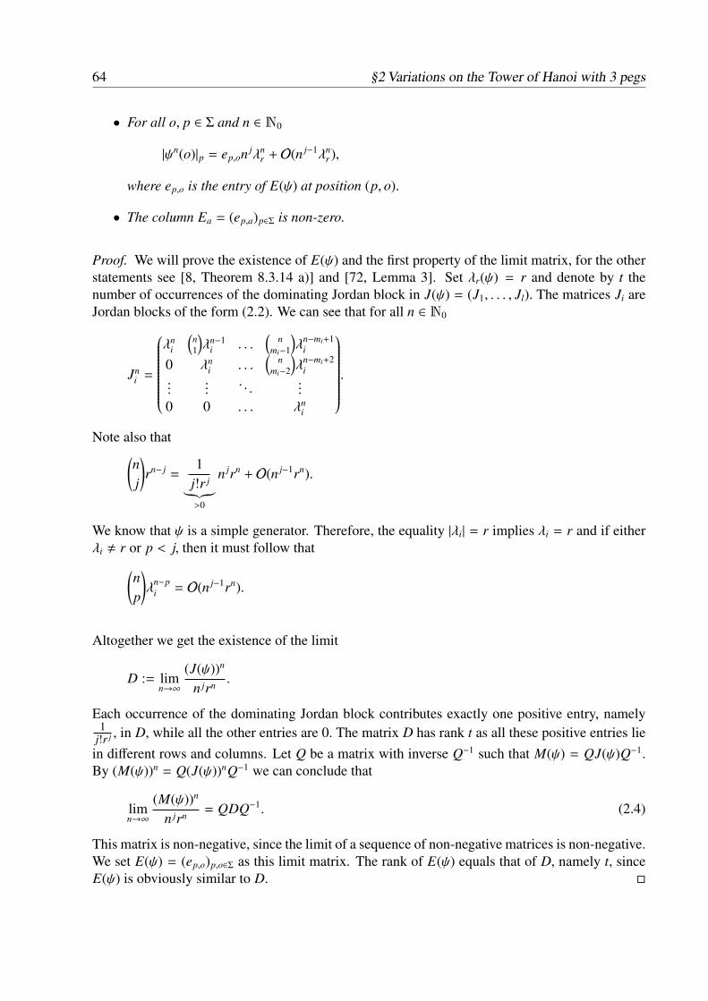
64 §2 Variations on the Tower of Hanoi with 3 pegs
• For all o, p ∈ Σ and n ∈ N0
|ψn(o)|p = ep,on jλnr + O(n j−1λn
r ),
where ep,o is the entry of E(ψ) at position (p, o).
• The column Ea = (ep,a)p∈Σ is non-zero.
Proof. We will prove the existence of E(ψ) and the first property of the limit matrix, for the otherstatements see [8, Theorem 8.3.14 a)] and [72, Lemma 3]. Set λr(ψ) = r and denote by t thenumber of occurrences of the dominating Jordan block in J(ψ) = (J1, . . . , Jl). The matrices Ji areJordan blocks of the form (2.2). We can see that for all n ∈ N0
Jni =
λn
i
(n1
)λn−1
i . . .(
nmi−1
)λn−mi+1
i
0 λni . . .
(n
mi−2
)λn−mi+2
i...
.... . .
...0 0 . . . λn
i
.Note also that(
nj
)rn− j =
1j!r j︸︷︷︸>0
n jrn + O(n j−1rn).
We know that ψ is a simple generator. Therefore, the equality |λi| = r implies λi = r and if eitherλi , r or p < j, then it must follow that(
np
)λ
n−pi = O(n j−1rn).
Altogether we get the existence of the limit
D := limn→∞
(J(ψ))n
n jrn .
Each occurrence of the dominating Jordan block contributes exactly one positive entry, namely1
j!r j , in D, while all the other entries are 0. The matrix D has rank t as all these positive entries liein different rows and columns. Let Q be a matrix with inverse Q−1 such that M(ψ) = QJ(ψ)Q−1.By (M(ψ))n = Q(J(ψ))nQ−1 we can conclude that
limn→∞
(M(ψ))n
n jrn = QDQ−1. (2.4)
This matrix is non-negative, since the limit of a sequence of non-negative matrices is non-negative.We set E(ψ) = (ep,o)p,o∈Σ as this limit matrix. The rank of E(ψ) equals that of D, namely t, sinceE(ψ) is obviously similar to D. �

§2 Variations on the Tower of Hanoi with 3 pegs 65
From the last lemma we deduce the following corollary. We let Mb = (mp,b)p∈∆ denote the columnof the matrix M = (mp,o)p∈∆
o∈Σthat corresponds to b ∈ Σ.
Corollary 2.20 ([72, Corollary 1]). Again, j+1 is the size of the dominating Jordan block in J(ψ).Define W(τ, ψ) := M(τ)E(ψ), where M(τ) is the incidence matrix of the coding τ and E(ψ) is thematrix from (2.3). Then
• For all o ∈ Σ, p ∈ ∆ and n ∈ N0,
|τ(ψn(o))|p = wp,on jλnr + O(n j−1λn
r ),
where wp,o is the entry of W(τ, ψ) at position (p, o).
• The column Wa is non-zero.
The following theorem guarantees the existence of the frequency of a letter.
Theorem 2.21. Let s = τ(ψ∞(a)) be a morphic sequence, where a ∈ Σ, ψ : Σ∗ → Σ∗ is a simplegenerator and τ : Σ∗ → ∆∗ is a coding. We will denote the matrix M(τ)E(ψ) by W(τ, ψ).The frequency of the letter q ∈ ∆ in s exists if and only if
wq,b∑p∈∆ wp,b
=wq,a∑
p∈∆ wp,a(2.5)
for all non-zero columns Wb of W(τ, ψ). If it exists, the frequency of q ∈ ∆ is the value in (2.5).
Proof. See [72, Theorem 2]. �
The next corollary arises from the last theorem and gives a necessary and sufficient condition forthe existence of the frequencies of all letters in morphic sequences.
Corollary 2.22 ([72, Corollary 2]). Under the hypotheses of Theorem 2.21, the frequencies existfor all letters in τ(ψ∞(a)) if and only if the rank of the matrix W(τ, ψ) equals one.
Proof. The frequencies of all letters exist if and only if (2.5) holds for every q ∈ ∆ and for allletters b ∈ Σ for which Wb is non-zero. We infer that this applies if and only if
Wb =
∑p∈∆ wp,b∑p∈∆ wp,a
Wa
for all non-zero columns Wb. (In [72], this is stated differently.) Since Wa is non-zero, this isequivalent to the condition that the rank of W(τ, ψ) is one and the proof is done. �
This completes the collection of the general tools we will need, and we can now proceed with ourspecial sequences.

66 §2 Variations on the Tower of Hanoi with 3 pegs
2.2.2 The T H(C+3 ) sequence
The permitted moves in T H(C+3 ) are the elements of ∆C+ := {a, b, c, a}. In [7], it is described that
the T H(C+3 ) sequence w is obtained as the image, under the coding κT , of the iterative fixed point
of the morphism ηT . Here the superscript T stands for temporary, since we will modify thembelow. Let ΣT
C+ be the set {x, r, z, t, u, s, a, b, c, a, b}. The map ηT : ΣT,∗C+→ ΣT,∗
C+is defined by
ηT (x) = rbasa, ηT (r) = rbaubr, ηT (z) = tau,ηT (t) = zbrb, ηT (u) = saczc, ηT (s) = sactas,ηT (a) = a, ηT (b) = b, ηT (c) = c,ηT (a) = a, ηT (b) = b,
and the coding κT : ΣT,∗C+→ ∆T,∗
C+is given by
κT (x) = a, κT (r) = a, κT (z) = a,κT (t) = b, κT (u) = c, κT (s) = c,κT (a) = a, κT (b) = b, κT (c) = c,κT (a) = a, κT (b) = b
with ∆TC+ := {a, b, c, a, b}. We see that the letter b is not an element of ∆C+ so that we delete it in
ΣTC+ and ∆T
C+. Referring to the proof of the next theorem, we will make another emendation. Thenew morphism is called η and the new coding κ with the sets ∆C+ and ΣC+.
Theorem 2.23. Let the map η : Σ∗C+ → Σ∗C+ be defined by
η(x) = rbasa, η(r) = rbaubr, η(z) = tau,η(t) = zbrb, η(u) = sacz, η(s) = sactas,η(a) = a, η(b) = b, η(c) = c,η(a) = a
and the coding κ : Σ∗C+ → ∆∗C+ be defined by
κ(x) = a, κ(r) = a, κ(z) = a,κ(t) = b, κ(u) = c, κ(s) = c,κ(a) = a, κ(b) = b, κ(c) = c,κ(a) = a
with ΣC+ := {x, r, z, t, u, s, a, b, c, a} and ∆C+ := {a, b, c, a}. Then the T H(C+3 ) sequence w is the
image, under the coding κ, of the iterative fixed point of the morphism η. In fact, w = κ(η∞(r)).
Proof. We define the following words on ∆C+ given by The Sapir Algorithm 7:
• Xn is the word to transfer n discs from peg 0 to peg 1,
• Yn is the word to transfer n discs from peg 0 to peg 2,
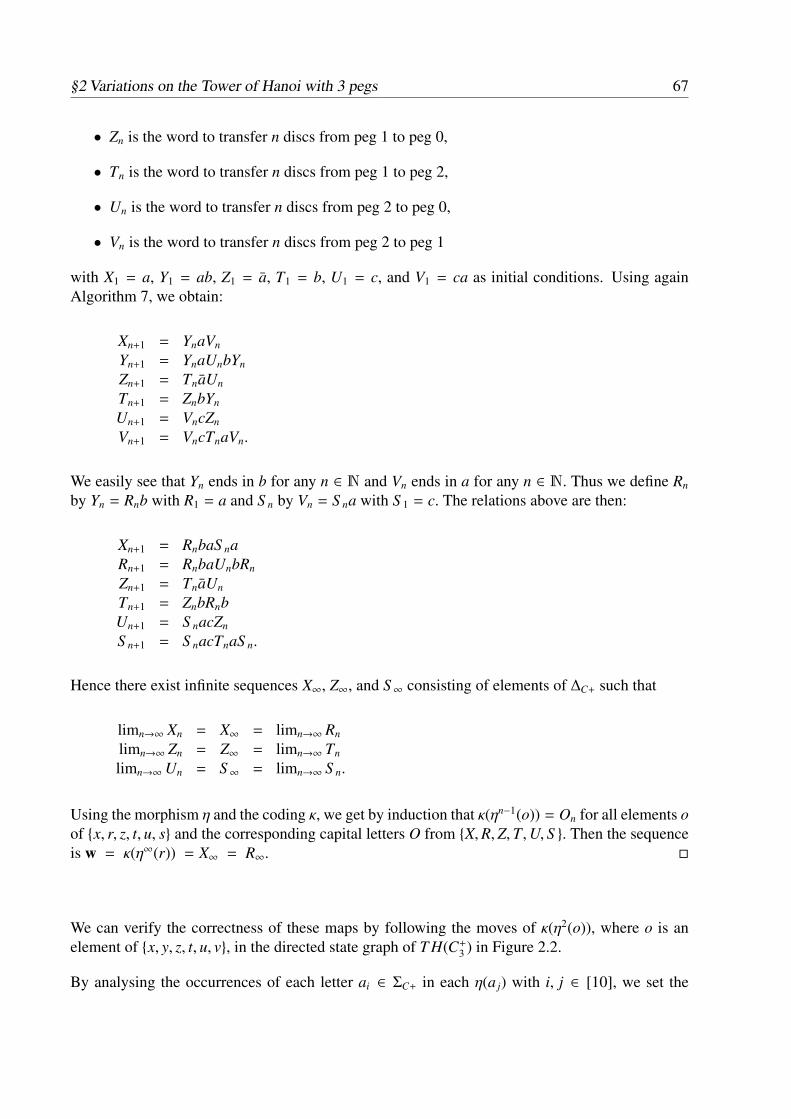
§2 Variations on the Tower of Hanoi with 3 pegs 67
• Zn is the word to transfer n discs from peg 1 to peg 0,
• Tn is the word to transfer n discs from peg 1 to peg 2,
• Un is the word to transfer n discs from peg 2 to peg 0,
• Vn is the word to transfer n discs from peg 2 to peg 1
with X1 = a, Y1 = ab, Z1 = a, T1 = b, U1 = c, and V1 = ca as initial conditions. Using againAlgorithm 7, we obtain:
Xn+1 = YnaVn
Yn+1 = YnaUnbYn
Zn+1 = TnaUn
Tn+1 = ZnbYn
Un+1 = VncZn
Vn+1 = VncTnaVn.
We easily see that Yn ends in b for any n ∈ N and Vn ends in a for any n ∈ N. Thus we define Rn
by Yn = Rnb with R1 = a and S n by Vn = S na with S 1 = c. The relations above are then:
Xn+1 = RnbaS naRn+1 = RnbaUnbRn
Zn+1 = TnaUn
Tn+1 = ZnbRnbUn+1 = S nacZn
S n+1 = S nacTnaS n.
Hence there exist infinite sequences X∞, Z∞, and S∞ consisting of elements of ∆C+ such that
limn→∞ Xn = X∞ = limn→∞ Rn
limn→∞ Zn = Z∞ = limn→∞ Tn
limn→∞Un = S∞ = limn→∞ S n.
Using the morphism η and the coding κ,we get by induction that κ(ηn−1(o)) = On for all elements oof {x, r, z, t, u, s} and the corresponding capital letters O from {X,R,Z,T,U, S }. Then the sequenceis w = κ(η∞(r)) = X∞ = R∞. �
We can verify the correctness of these maps by following the moves of κ(η2(o)), where o is anelement of {x, y, z, t, u, v}, in the directed state graph of T H(C+
3 ) in Figure 2.2.
By analysing the occurrences of each letter ai ∈ ΣC+ in each η(a j) with i, j ∈ [10], we set the
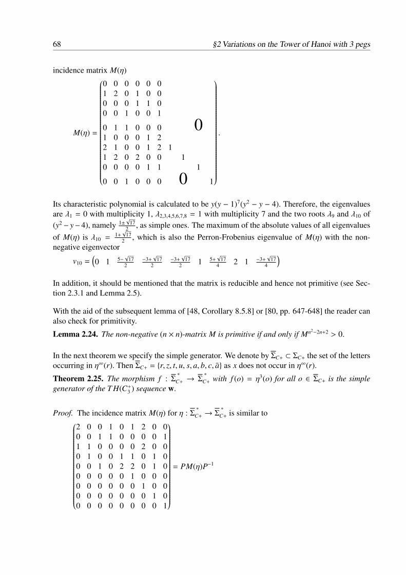
68 §2 Variations on the Tower of Hanoi with 3 pegs
incidence matrix M(η)
M(η) =
0 0 0 0 0 01 2 0 1 0 00 0 0 1 1 00 0 1 0 0 1
0 1 1 0 0 0 01 0 0 0 1 22 1 0 0 1 2 11 2 0 2 0 0 10 0 0 0 1 1 1
0 0 1 0 0 0 0 1
.
Its characteristic polynomial is calculated to be y(y − 1)7(y2 − y − 4). Therefore, the eigenvaluesare λ1 = 0 with multiplicity 1, λ2,3,4,5,6,7,8 = 1 with multiplicity 7 and the two roots λ9 and λ10 of(y2 − y− 4), namely 1±
√17
2 , as simple ones. The maximum of the absolute values of all eigenvaluesof M(η) is λ10 = 1+
√17
2 , which is also the Perron-Frobenius eigenvalue of M(η) with the non-negative eigenvector
v10 =(0 1 5−
√17
2−3+
√17
2−3+
√17
2 1 5+√
174 2 1 −3+
√17
4
)In addition, it should be mentioned that the matrix is reducible and hence not primitive (see Sec-tion 2.3.1 and Lemma 2.5).
With the aid of the subsequent lemma of [48, Corollary 8.5.8] or [80, pp. 647-648] the reader canalso check for primitivity.
Lemma 2.24. The non-negative (n × n)-matrix M is primitive if and only if Mn2−2n+2 > 0.
In the next theorem we specify the simple generator. We denote by ΣC+ ⊂ ΣC+ the set of the lettersoccurring in η∞(r). Then ΣC+ = {r, z, t, u, s, a, b, c, a} as x does not occur in η∞(r).
Theorem 2.25. The morphism f : Σ∗
C+ → Σ∗
C+ with f (o) = η3(o) for all o ∈ ΣC+ is the simplegenerator of the T H(C+
3 ) sequence w.
Proof. The incidence matrix M(η) for η : Σ∗
C+ → Σ∗
C+ is similar to
2 0 0 1 0 1 2 0 00 0 1 1 0 0 0 0 11 1 0 0 0 0 2 0 00 1 0 0 1 1 0 1 00 0 1 0 2 2 0 1 00 0 0 0 0 1 0 0 00 0 0 0 0 0 1 0 00 0 0 0 0 0 0 1 00 0 0 0 0 0 0 0 1
= PM(η)P−1

§2 Variations on the Tower of Hanoi with 3 pegs 69
by
P =1
16
16 0 0 0 0 0 0 0 0−9 18 −11 −11 −9 16 0 −16 32−17 −14 −3 −3 −17 0 16 16 16−4 −8 4 4 −4 0 0 16 01 −2 3 3 1 0 0 16 −16
16 16 0 0 16 16 −16 −48 16−6 −4 6 −2 −6 −8 8 16 −8−12 −24 −4 12 4 −32 16 64 −32
8 32 8 8 8 16 −16 −48 16
.
The submatrices A2,2 = A3,3 = A4,4 = A5,5 =(1)
of PM(η)P−1, named as in the proof of The-orem 2.18, are irreducible, as is
A1,1 =
2 0 0 1 00 0 1 1 01 1 0 0 00 1 0 0 10 0 1 0 2
.
The square matrix A1,1 is even primitive as we calculate A41,1 > 0.
The integer h from the proof of Theorem 2.18, which is the least common multiple of all indicesof the Ai,is, is 1, since the characteristic polynomial of A1,1 is (y−1)3(y2−y−4) and thus h1 = 1.Wedefine the morphism f : Σ
∗
C+ → Σ∗
C+ from the condition f (r) = ηhl(r) = ηl(r). To find l, we apply ηon r until every letter of ΣC+ occurs in the result. We get l = 3 and, consequently, f = η3(r). Thus(G1) is satisfied. We determine the mapping rules of the letters under f .
We find that
f (r) = η3(r) = rbaubrbasaczbrbaubrbasactasactaubrbaubrbasaczbrbaubr,
f (z) = η3(z) = taubrbaubrbasactasactau,f (t) = η3(t) = zbrbasaczbrbaubrbasaczbrbaubrb,f (u) = η3(u) = sactasaczbrbasactasaczbrbasacz,f (s) = η3(s) = sactasaczbrbasactasactaubrbaubr
basactasaczbrbasactas,f (a) = η3(a) = a, f (c) = η3(c) = c,f (b) = η3(b) = b, f (a) = η3(a) = a.
Since η is a morphism, f is also a morphism.

70 §2 Variations on the Tower of Hanoi with 3 pegs
As incidence matrix of f we get
M( f ) =
8 2 5 2 42 0 3 3 22 3 0 2 5
5 3 2 0 2 04 2 2 5 8
12 4 5 8 15 114 4 10 4 8 14 2 2 5 7 1
1 3 1 1 1 0 1
.
The characteristic polynomial equals (t − 1)7(t2 − 13t − 64). This gives nine eigenvalues, namelyλ1,2,3,4,5,6,7 = 1 with multiplicity 7 and λ8 = 13−5
√17
2 and λ9 = 13+5√
172 both with multiplicity one.
The eigenvalue with the maximal absolute value is the Perron-Frobenius eigenvalue, here λ9, withthe non-negative eigenvector
v9 =(1 5−
√17
2−3+
√17
2−3+
√17
2 1 5+√
174 2 1 −3+
√17
4
).
All other eigenvalues of M( f ) have absolute values which are not equal to λ9. Hence (G2) isfulfilled. �
The Jordan block corresponding to λ9 occurs only once in the Jordan form of M( f ), since
Q−1M( f )Q =
λ8
1 10 1
1 1
0 1 01
1
0 1λ9
,
where Q is an invertible matrix. The Jordan blocks are J1 = (λ8), J4 = J5 = J6 = (1), J7 = (λ9),and
J2 = J3 =
(1 10 1
).
This clearly implies j = 0, since j + 1 is the size of the dominating Jordan block J6. We calculatethe matrix Q, which is the one which has the eigenvectors of λ8 and λ9 as first and last column,respectively, such that

§2 Variations on the Tower of Hanoi with 3 pegs 71
Q =
1 3 1 0 0 1 0 0 1a 0 0 0 1 0 0 0 eb −3 0 0 0 −1 0 0 fb 3 0 0 1 1 0 0 f1 −3 −1 0 −1 −1 0 0 1c −3 0 −3 0 0 1 0 g2 6 0 0 0 0 0 1 21 −3 0 0 0 0 0 0 1d 0 0 3 0 0 0 0 h
,
where the roman letters in Q stand for
a =√
17+52 , e = −
√17−52 ,
b = −√
17+32 , f =
√17−32 ,
c = −√
17−54 , g =
√17+54 ,
d = −√
17+34 , h =
√17−34 .
With the last results we compute the matrix E( f ) from Lemma 2.19. The limit
E( f ) = limn→∞
(M( f ))n
λn9
= limn→∞
Q(
J( f )λ9
)︸ ︷︷ ︸
=:B
n
Q−1
exists with
Bn =1λn
9
λn8
1n(
n1
)1n−1
0 1n
1n(
n1
)1n−1 0
0 1n
1n
1n
0 1n
λn9
.
This yields E( f ) = Q
01
Q−1, where the (1)-matrix has dimension 1 × 1 and lies on the
diagonal. The incidence matrix of the coding κ is given by
M(κ) =
1 0 0 0 0 1 0 0 00 0 1 0 0 0 1 0 00 0 0 1 1 0 0 1 00 1 0 0 0 0 0 0 1
.

72 §2 Variations on the Tower of Hanoi with 3 pegs
From what has already been proved, we calculate the (4 × 9)-matrix
W(κ, f ) = M(κ)E( f ). (2.6)
With (2.6) we obtain
Theorem 2.26. The frequency of the letter a in w exists and has the value
Freqa(w) =17 + 9
√17
68.
Proof. Recall that f is prolongable on the letter r of ΣC+. We calculate
F := wa,r∑p∈∆C+
wp,r=
g+1e+2f+g+h+5
=14
(√17+9
)√
17
= 17+9√
1768
(2.7)
as the candidate for the frequency of a ∈ ∆C+, according to Theorem 2.21. By the same theorem,it remains to prove that
wa,k∑p∈∆C+
wp,k=
wa,r∑p∈∆C+
wp,r
for all non-zero columns Wk of W(κ, f ). We have
wa,k∑p∈∆C+
wp,k=
g+1σ
for all k ∈ {z, t, u, s} and σ := e + 2f + g + h + 5. All these numbers are equal to F of (2.7) so thatFreqa(w) = F. �
By virtue of Corollary 2.22, the frequencies of all letters in ∆C+ actually exist, since the rank ofW(κ, f ) equals one. A trivial calculation with Sage shows that
Freqb(w) = f+2σ
=√
17+12√
17=√
17+1734 ,
Freqc(w) = f+2σ
=√
17+1734 ,
Freqa(w) = e+hσ
= −√
17+74√
17= 7
√17−1768 .
All these frequencies of letters in ∆C+ are not rational. From Theorem 2.13 we know that if asequence is d-automatic for any d, then, assuming its existence, the frequency of a letter in thissequence has to be rational . Hence we proved now that
Theorem 2.27. For any d ∈ N2 the T H(C+3 ) sequence w is not d-automatic.

§2 Variations on the Tower of Hanoi with 3 pegs 73
2.2.3 The T H(K−3 ) sequence
With a view to Figure 2.1, we get the allowed moves in T H(K−3 ). These moves can be summarisedin the set ∆K− := {a, b, c, a, b}. By definition, a sequence is morphic if it can be obtained as theimage, under a coding, of an iterative fixed point of a morphism. For the T H(K−3 ) sequence u amorphism φ : {x, y, z, d, e, f , a, b, c, a, b} → {x, y, z, d, e, f , a, b, c, a, b} is defined by
φ(x) = yba f , φ(y) = ybaeby, φ(z) = dae,φ(d) = zbyb, φ(e) = f cz, φ( f ) = ebx,φ(a) = a, φ(b) = b, φ(c) = c,φ(a) = a, φ(b) = b,
and the corresponding coding, under the map
τ : {x, y, z, d, e, f , a, b, c, a, b} → ∆K−,
is given by
τ(x) = a, τ(y) = a, τ(z) = a,τ(d) = b, τ(e) = c, τ( f ) = b,τ(a) = a, τ(b) = b, τ(c) = c,τ(a) = a, τ(b) = b.
The finite alphabet {x, y, z, d, e, f , a, b, c, a, b} is called ΣK−.
Theorem 2.28 ([7, Theorem 2]). The T H(K−3 ) sequence u is the image, under the coding τ, of theiterative fixed point of the morphism φ, in particular u = τ(φ∞(y)).
Proof. We define the following words on ∆K− given by The Sapir Algorithm 7:
• Xn is the word to transfer n discs from peg 0 to peg 1,
• S n is the word to transfer n discs from peg 0 to peg 2,
• Zn is the word to transfer n discs from peg 1 to peg 0,
• Dn is the word to transfer n discs from peg 1 to peg 2,
• En is the word to transfer n discs from peg 2 to peg 0,
• Fn is the word to transfer n discs from peg 2 to peg 1
with X1 = a, S 1 = ab, Z1 = a, D1 = b, E1 = c, and F1 = b as initial conditions. Using againAlgorithm 7, we obtain:
Xn+1 = S naFn
S n+1 = S naEnbS n
Zn+1 = DnaEn
Dn+1 = ZnbS n
En+1 = FncZn
Fn+1 = EnbXn.

74 §2 Variations on the Tower of Hanoi with 3 pegs
We easily see that S n ends in b for any n ∈ N. Thus we define Yn by S n = Ynb with Y1 = a.The relations above are then:
Xn+1 = YnbaFn
Yn+1 = YnbaEnbYn
Zn+1 = DnaEn
Dn+1 = ZnbYnbEn+1 = FncZn
Fn+1 = EnbXn.
Hence there exist infinite sequences X∞, Z∞, and E∞ consisting of elements of ∆K− such that
limn→∞ Xn = X∞ = limn→∞ S n = limn→∞ Yn
limn→∞ Zn = Z∞ = limn→∞ Dn
limn→∞ En = E∞ = limn→∞ Fn.
Using the morphism φ and the coding τ, we get by induction that τ(φn−1(o)) = On for all elementso of {x, y, z, d, e, f } and corresponding capital letters O in {X,Y,Z,D, E, F}. Then the sequence isu = τ(φ∞(y)) = X∞. �
Again, we can verify the correctness of these maps by following the moves of τ(φ2(o)), where theletter o is an element of {x, s, z, d, e, f } in the directed state graph of T H(K−3 ) in Figure 2.2.
For the incidence matrix of φ we get
M(φ) =
0 0 0 0 0 11 2 0 1 0 00 0 0 1 1 0
0 0 1 0 0 0 00 1 1 0 0 11 0 0 0 1 01 1 0 0 0 0 11 2 0 2 0 0 10 0 0 0 1 0 1
0 0 1 0 0 0 0 10 0 0 0 0 1 1
. (2.8)
Its characteristic polynomial is given by (t + 1)(t − 1)7(t3 − t2 − 4t + 2). Hence the eigenvaluesare λ1 = −1 with multiplicity 1, λ2,3,4,5,6,7,8 = 1 with multiplicity 7 and the three roots λ9, λ10, λ11
(ordered by ascending absolute value) of (t3 − t2 − 4t + 2) as simple ones. The maximum of theabsolute values of all eigenvalues of M(φ) is the maximal root λ11 of (t3 − t2 − 4t + 2). This root istherefore also the Perron-Frobenius eigenvalue of M(φ).
Note that this matrix is again reducible and not primitive (see Section 2.3.1 and Lemma 2.24).

§2 Variations on the Tower of Hanoi with 3 pegs 75
The following theorem specifies the simple generator for u. The set ΣK− is the set of letters whichoccur in η∞(y). Here, ΣK− is equal to ΣK−.
Theorem 2.29. The morphism g : Σ ∗K− → Σ ∗K− with g(o) = φ3(o) for all o ∈ ΣK− is a simplegenerator for the T H(K−3 ) sequence u.
Proof. The matrix M(φ) can be transformed in the following way
M(φ) ∼
0 1 0 0 0 1 1 1 0 0 00 2 0 0 1 0 1 2 0 0 00 0 0 1 1 0 0 0 0 1 00 1 1 0 0 0 0 2 0 0 00 0 1 0 0 1 0 0 1 0 01 0 0 0 1 0 0 0 0 0 1
11
0 11
1
,
since M(φ) is similar to its transpose.
We show briefly that every square matrix A is similar to its transpose. Let J(A) be the matrix inJordan form of A. Thus Q−1AQ = J(A) for an invertible matrix Q and
J(A)T = QT AT (Q−1)T = QT AT (QT )−1.
It follows that J(A)T is similar to AT . Using the transitive property of similarity, it is sufficientto prove that J(A)T is similar to J(A). Because of the block decomposition of J(A), we haveonly to show that any Jordan block J(A)i is similar to its transpose. This can be seen easily. Infact, if P is the permutation matrix with a line of 1s from top right to bottom left, then we getPJ(A)iP−1 = (J(A)i)T .
The submatrices A2,2 = A3,3 = A4,4 = A5,5 = A6,6 =(1)
are irreducible and so is
A1,1 =
0 1 0 0 0 10 2 0 0 1 00 0 0 1 1 00 1 1 0 0 00 0 1 0 0 11 0 0 0 1 0
,
since A61,1 > 0. The characteristic polynomial of A1,1 is (t + 1)(t − 1)2(t3 − t2 − 4t + 2). It fol-
lows that the index of A1,1 equals 1. Therefore, the integer h from the proof of Theorem 2.18 is

76 §2 Variations on the Tower of Hanoi with 3 pegs
h = lcm (1, 1, . . . , 1) = 1. Now we are able to find a morphism g : Σ ∗K− → Σ ∗K− with the conditiong(y) = φhl(y) = φl(y). But what is l ∈ N? Every letter of ΣK− has to occur in φl(y). By an easycalculation, we see that l = 3 and, consequently, g = φ3(y). We determine the new mapping rulesunder g for every letter of ΣK−
g(y) = φ3(y) = ybaebyba f czbybaebybaebxcdaebybaebyba f czbybaeby,
g(x) = φ3(x) = ybaebyba f czbybaebyba f czbyba f ,g(z) = φ3(z) = daebybaebybaebxcdae,g(d) = φ3(d) = zbyba f czbybaebyba f czbybaebyb,g(e) = φ3(e) = f czbyba f czbyba f cz,g( f ) = φ3( f ) = ebxcdaebybaebybaebx,g(a) = φ3(a) = a, g(a) = φ3(a) = a,g(b) = φ3(b) = b, g(b) = φ3(b) = b,g(c) = φ3(c) = c.
It is obvious that g is a morphism and that (G1) is satisfied.
We must again specify an incidence matrix, but this time for the simple generator g. It is
M(g) =
0 1 1 0 0 25 8 2 5 2 22 2 0 3 3 0
0 1 2 0 0 1 02 6 4 2 0 43 2 0 2 3 05 7 1 3 1 2 18 14 4 10 3 3 12 3 1 2 3 1 1
0 1 3 1 1 1 0 11 1 1 0 1 3 1
.
As the characteristic polynomial of M(g) we get
t11 − 13t10 − 20t9 + 352t8 − 1014t7 + 1190t6
−224t5 − 960t4 + 1133t3 − 561t2 + 124t − 8= (t − 1)7(t + 1)(t3 − 7t2 − 76t + 8).
We immediately see that 1 and −1 are the eigenvalues with multiplicity 7 and 1, respectively, butthese are not all. We further detect the three roots of t3 − 7t2 − 76t + 8 = at3 + bx2 + ct + d byCardano’s method ([19]). From
p = − b2
3a2 + ca = −277
3q = d
a −bc3a2 + 2b3
27a3 = −525827

§2 Variations on the Tower of Hanoi with 3 pegs 77
we calculate the discriminant D =p3
27 +q2
4 = −53119627 < 0. Hence there are three real roots and we
are in the “casus irreducibilis”. With [19, p.78 ff.] the roots are
t1 = 2√
2779 cos
(13 arccos
(4732214958
√9
277 −2π3
))+ 7
3 ,
t2 = 2√
2779 cos
(13 arccos
(4732214958
√9
277 − 22π3
))+ 7
3 ,
t3 = 2√
2779 cos
(13 arccos
(4732214958
√9
277
))+ 7
3 ,
It follows that t3 is the Perron-Frobenius eigenvalue of M(g). The condition (G2) is fulfilled as t3
itself is the only eigenvalue of M(g) whose absolute value equals t3. �
We are interested in finding the Jordan matrix decomposition of M(g). There exists an invertiblesquare matrix Q such that M(g) = QJ(g)Q−1, where
J(g) =
t1
−1
t2 01 10 1
1 10 1
1
0 11
t3
is the matrix in Jordan form. We have nine Jordan blocks, namely
J1 = (t1), J2 = (−1), J3 = (t2), J4 = J5 =
(1 10 1
), J6 = J7 = J8 = (1), and J9 = (t3).
It is easily seen that the dominating Jordan block of M(g) is J9, which implies j + 1 = 1 as its size.By the definition of E(g) in Lemma 2.19, this yields
E(g) = limn→∞
(M(g))n
tn3
= limn→∞
Q(
J(g)t3
)︸ ︷︷ ︸
=:B
n
Q−1 = limn→∞
QBnQ−1.

78 §2 Variations on the Tower of Hanoi with 3 pegs
The task is to find Bn in order to evaluate the limit. Bn is given by
Bn =1tn3
tn1
(−1)n
tn2 0
1n(
n1
)1n−1
0 1n
1n(
n1
)1n−1
0 1n
1n
1n
0 1n
1n
tn3
.
We thus get
E(g) = Q(limn→∞
Bn)
Q−1 = Q
01
Q−1,
where the (1)-matrix has dimension 1 × 1 and lies on the diagonal.
The invertible matrix Q has the form Q = [v1 . . . v2 . . . v3] where vi are the eigenvectors of ti
(i = 1, 2, 3). We calculate Q with the algebra system Sage and see that
Q =
1 1 1 0 1 0 0 0 0 0 1a 0 h 0 0 0 1 0 0 0 ob 1 i 0 −1 0 −1 0 0 0 p1 −1 1 0 −1 0 −1 0 0 0 1c 0 j 0 0 0 0 0 0 0 qb −1 i 0 1 0 0 0 0 0 pd −1
2 k 3 0 3 0 1 0 0 re 1
2 l −3 0 0 0 0 1 0 sf 0 m 0 0 0 0 0 0 1 tg −1
2 n −3 0 −3 0 0 0 0 ug 1
2 n 3 0 0 0 0 0 0 u
. (2.9)
The first column is v1, the third one v2 and the last one v3. Note that the roman letters in thismatrix are not related to the elements of ΣK−. By now, there is only one part missing to constructthe matrix W(τ, g) of Corollary 2.20 and consequently the frequency of a letter of ΣK−, namely tofind the incidence matrix of the coding τ. We see that
M(τ) =
1 1 0 0 0 0 1 0 0 0 00 0 0 1 0 0 0 1 0 0 00 0 0 0 1 0 0 0 1 0 00 0 1 0 0 0 0 0 0 1 00 0 0 0 0 1 0 0 0 0 1
.

§2 Variations on the Tower of Hanoi with 3 pegs 79
We are now in a position to determine W(τ, g). By definition, the matrix W(τ, g) is equal to the(5 × 11)-matrix M(τ)E(g). From this we get
Theorem 2.30. The frequency of the letter a ∈ ∆K− in u exists and is equal to
Freqa(u) =(o + r + 1)
(o + 2p + q + r + s + t + 2u + 2),
where the roman letters are the numbers as defined in the matrix Q in (2.9).
Proof. Recall that g is prolongable on the letter y of ΣK−. As candidate for the frequency of theletter a ∈ ∆K− we obtain
G := wa,y∑p∈∆K− wp,y
=(o+r+1)
(o+2p+q+r+s+t+2u+2) (2.10)
according to Theorem 2.21. We see that
wa,y∑p∈∆K− wp,y
=wa,k∑
p∈∆K− wp,k
for all non-zero columns Wk of W(τ, φ). Finally, we conclude that the frequency of the lettera ∈ ∆K− in τ(g∞(y)) exists and is equal to G. �
It remains to see whether the number G is rational or not. In the case of rationality we couldconclude that the sequence u is possibly d-automatic for some d, while in the opposite case itcannot be d-automatic for any d. Unfortunately, we cannot determine whether the expression(2.10) is irrational because of its complexity. Hence we will try another approach to disprove theautomaticity of this sequence in the next section.
2.3 A new approach to disprove the automaticity of the T H(K−3 )sequence
As in the previous section, we define the set of allowed moves in T H(K−3 ) as ∆K− := {a, b, c, a, b}.Then the T H(K−3 ) sequence u is the image, under the coding
τ : {x, y, z, d, e, f , a, b, c, a, b} → {a, b, c, a, b}
given by
τ(x) = a, τ(y) = a, τ(z) = a,τ(d) = b, τ(e) = c, τ( f ) = b,τ(a) = a, τ(b) = b, τ(c) = c,τ(a) = a, τ(b) = b,

80 §2 Variations on the Tower of Hanoi with 3 pegs
of the fixed point of the morphism φ : Σ∗K− → Σ∗k− defined by
φ(x) = yba f , φ(y) = ybaeby, φ(z) = dae,φ(d) = zbyb, φ(e) = f cz, φ( f ) = ebx,φ(a) = a, φ(b) = b, φ(c) = c,φ(a) = a, φ(b) = b.
The set ΣK− := {x, y, z, d, e, f , a, b, c, a, b} is a finite alphabet. Then our sequence is u = τ(φ∞(y)).
The new approach to decide whether the sequence u is automatic or not is the use of Cobham’sTheorem [17], which makes a statement about the ultimate periodicity of sequences under certainconditions. The idea of the application of this theorem was already outlined in [7] and again dis-cussed during a private communication between Allouche and the author of the present thesis [3].For the formulation of that theorem we need some preparations. Let x and y be finite words. Thenwe call an infinite sequence s of the form xy∞,where y , ε and y∞ = yyy . . . , ultimately periodic10.If x is the empty word, the sequence is called periodic.
One calls two integers p, q ∈ N1 multiplicatively independent if no positive integers α and β existsuch that pα = qβ.Otherwise p and q are multiplicatively dependent. The next lemma characterisesthis property.
Lemma 2.31 ([8, Theorem 2.5.7]). Let p, q ∈ N2. The following statements are equivalent:
a) p and q are multiplicatively dependent.
b) logp q is rational.
c) logq p is rational.
d) There exist an integer n ∈ N2 and two integers x, y ∈ N such that p = nx and q = ny.
Theorem 2.32 (Cobham’s Theorem, [17]). Let p and q be multiplicatively independent integersand let s be a sequence which is both p- and q-automatic. Then s is ultimately periodic.
Next, we show that if the sequence u is not ultimately periodic, then we can conclude that u is notd-automatic for any d ∈ N2.
Why can we conclude this? [7, Proposition 1] tells us that the Perron-Frobenius eigenvalue of theincidence matrix M(φ) of the T H(K−3 ) sequence and any integer d ∈ N are multiplicatively inde-pendent. We prove this statement more extensively in the next lemma with the aid of Lemma 2.31and an algebraic argument (for the theory about field extensions; see for instance [29]).
Lemma 2.33. Let λr (∈ N1) be the maximal root of the polynomial (t3 − t2 − 4t + 2). Then for any
d ∈ N the real number logd λr =ln λr
ln dis irrational.
10Recall the remark in Section 2.1. A sequence is 1-automatic if and only if it is ultimately periodic (see [8, Theorem5.7.1]).

§2 Variations on the Tower of Hanoi with 3 pegs 81
Proof. We assume that logd λr = nm with positive integers m, n. Then d
nm = λr, which implies
dn = λmr . Since dn is an integer, it is sufficient to show that for any m ∈ N the numbers λm
r are notintegers. For this purpose we use the following argument. Suppose α := λm
r is an integer. We caneasily see that λr is algebraic over Q. Now let I be the set of all polynomials P over Q such thatP(λr) = 0. I is an ideal of Q[T ], where Q[T ] is the polynomial ring over Q. As Q is a field, Q[T ]is a principal ideal domain and, therefore, I consists of all polynomial multiples over Q of somem(t) ∈ Q[T ]. Since (t3− t2−4t + 2) has no rational root, it is irreducible over Q, and it follows thatm(t) = t3 − t2 − 4t + 2. Then, since λr is also a root of (tm −α) and (tm −α) ∈ Q[T ], the polynomial(t3−t2−4t+2) divides (tm−α), i.e., there exists a polynomial Q(t) = am−3tm−3+. . .+a1t+a0 ∈ Q[T ]such that
(t3 − t2 − 4t + 2)Q(t) = tm − α. (2.11)
If ai = ri/si for ri, si ∈ Z with i ∈ [m − 2]0 and if we let s = lcm(s0, . . . , sm−3), then we can writeQ(t) = s−1Q′(t) where Q′(t) ∈ Z[T ]. Hence we can assume that Q(t) is a polynomial with integercoefficients. We reduce Equation (2.11) modulo 2
t2(t − 1)Q(t) ≡ tm − α mod 2.
Then, if we set t mod 2 = 0, the integer α mod 2 = 0. However, if we set t mod 2 = 1, theinteger α mod 2 = 1, which is a contradiction. �
Assuming that u is not ultimately periodic, it would follow with the previous lemma that for anyd ∈ N the sequence u is not d-automatic. Hence it remains to prove whether the sequence is notultimately periodic. The decidability of the question whether an infinite sequence is ultimatelyperiodic, called the HD0L11 ultimate periodicity problem, has been an open problem for a longtime.
As described in the introduction, first steps were done for special types of sequences. F. Dur-and [25] solved the problem in the case that the morphism is primitive in 2012. Shortly thereafter,he proved the decidability of the whole problem [26].
At around the same time, I. V. Mitrofanov presented two other proofs of the decidability of theHD0L ultimate periodicity problem. The first proof was published as a preprint [62] and accordingto Mitrofanov it is based on the paper [51]. In the sequel we will make use of the second proofin [63].
In the first subsection we will employ the proof in F. Durand’s paper [26] and continue after theappearance of difficulties in the exact calculation with the one of I. V. Mitrofanov [63] in thesecond subsection.
11A D0L system is a triple G = (A, ψ, a) where A is a finite alphabet, ψ : A∗ → A∗ is an endomorphism and a is a wordin A∗. An HD0L system is a 5-tuple G = (A, B, ψ, τ, a) where (A, ψ, a) is a D0L system, B is a finite alphabet andτ : A∗ → B∗ is a morphism. If τ(ψn(a)) converges (for the usual product topology on AN) as n tends to infinity,we call the limit a HD0L sequence. For further reading about HD0L sequences we refer to [25].

82 §2 Variations on the Tower of Hanoi with 3 pegs
2.3.1 F. Durand’s method about the ultimate periodicity of (primitive) sequences
We formulate the problem explicitly: given two finite alphabets A and B, a morphism ψ : A∗ → A∗,a word a ∈ A∗, and a morphism τ : A∗ → B∗, is the sequence τ(ψ∞(a)) ultimately periodic?
From the last section we know that M(φ) is not primitive and, accordingly, φ is not primitiveeither. Hence we apply the results of the article [26]. Our procedure is to display statementsof [26] successively, immediately deducing the derivable results for our sequence.
We will state the first proposition, which is based on [26, Corollary 3.3] or [27, Proposition 5].
The alphabet A, over which ψ is defined, can be partitioned such that a power of the incidencematrix M(ψ) has a special form which is described in the subsequent proposition.
Proposition 2.34. Let P = (pi, j)i, j∈A be a matrix with non-negative coefficients. Then there existthree positive integers r, s, and t, where s ≤ t − 1, and a partition
{A j : j ∈ [t]
}of A such that
Pr =
A1 A2 . . . As As+1 As+2 . . . At
P1 0 . . . 0 0 0 . . . 0P2,1 P2 . . . 0 0 0 . . . 0...
.... . .
......
......
...Ps,1 Ps,2 . . . Ps 0 0 . . . 0
Ps+1,1 Ps+1,2 . . . Ps+1,s Ps+1 0 . . . 0Ps+2,1 Ps+2,2 . . . Ps+2,s 0 Ps+2 . . . 0...
.... . .
......
.... . .
...Pt,1 Pt,2 . . . Pt,s 0 0 . . . Pt
A1
A2...As
As+1
As+2...At
and the submatrices P j, corresponding to the subsets A j of A, have only positive entries or are thezero matrix.
With Lemma 2.24 and [59, Sections 4.4 and 4.5] about the irreducible components of non-negativematrices and the cyclic structures of irreducible matrices, the partition and r can be computedalgorithmically.
We demonstrate the procedure as applied in our context. Recall M(φ) of (2.8). There is a multidi-graph G(φ) associated with M(φ) whose vertex set is ΣK− and edge set consists of M(φ)IJ distinctarcs with initial vertex I and terminal vertex J. We say that I ∼ J if there exists a path in G(φ) fromI to J. Then I communicates with J if I ∼ J and J ∼ I. This is an equivalence relation. (The proofis left to the reader.) The communicating classes partition the set ΣK− as these are the maximalsets of vertices such that each one communicates with all the others in the class.
By drawing the associated graph, we get six communicating classes A1 = {x, y, z, d, e, f } andA2, A3, A4, A5, A6 with one element of ∆K− each.
If we read these classes again as vertices and draw an arc from class Ai to class A j if and only ifAi , A j and there is an arc in G(φ) with some element in Ai as initial vertex and some element in

§2 Variations on the Tower of Hanoi with 3 pegs 83
A j as terminal vertex, we get a graph H. Note that H is a digraph. This graph of communicatingclasses has only one sink, i.e., a vertex Av such that no arc leaves Av. By removing this sink, wecan order the classes such that there can be a path in H from Ai to A j only if j > i. When wearrange the vertices in the corresponding order, we get the block triangular form
M(φ) =
M1 0 0 0 0 0∗ M2 0 0 0 0∗ ∗ M3 0 0 0∗ ∗ ∗ M4 0 0∗ ∗ ∗ ∗ M5 0∗ ∗ ∗ ∗ ∗ M6
=
0 0 0 0 0 11 2 0 1 0 00 0 0 1 1 0
0 0 1 0 0 0 00 1 1 0 0 11 0 0 0 1 01 1 0 0 0 0 11 2 0 2 0 0 10 0 0 0 1 0 1
0 0 1 0 0 0 0 10 0 0 0 0 1 1
,
where ∗ are submatrices. We denote by Gi the subgraph of G with vertex set Ai and whose arcsare those of G whose initial and terminal vertices are in Ai. These graphs Gi associated withthe matrices Mi are called the irreducible components of G(φ). They are irreducible as they arerespectively strongly connected.
Remark. A matrix A is irreducible if and only if the multidigraph G(A) associated with A isstrongly connected, i.e., if for any pair of distinct vertices a and b there exists a directed pathfrom a to b and a directed path from b to a. We give only a sketch of the proof. Assume that A isreducible, then there exists a permutation matrix P such that
A = P(A1 R0 A2
)P−1 = PAP−1.
The multidigraph associated with A cannot be strongly connected, since the vertices correspondingto the lower left part of A are not connected. As the graphs G(A) and G(A) are isomorphic, G(A)is not strongly connected. Now suppose that G(A) is not strongly connected, i.e., there exist non-empty sets S and S ′ such that no directed path from one vertex of S to one of S ′ exists. Relabelthe vertices of G(A) as elements of S and S ′ and permute the matrix A in the same manner to getA. The new graph is G(A). As there are no directed paths from one vertex in S to one in S ′, wededuce that A must have a block of zeros in the lower left corner. Hence A is reducible. Since Aand A are permutationally similar, we see that A is irreducible.
We will see that each irreducible matrix has a characteristic period p.Let A be a non-negative matrix. The set of vertices in the graph associated with A is equal tothe set of states of A. The period per(I) of a state I is, by definition, the greatest common divisorof all those integers m ∈ N for which (Am)II > 0. In the case that no such integer exists, we setper(I) = ∞. The period per(A) of a matrix A is the greatest common divisor of all finite numbersper(I), or is∞ if per(I) = ∞ for all I. We call a matrix A aperiodic if per(A) = 1.

84 §2 Variations on the Tower of Hanoi with 3 pegs
Lemma 2.35 ([59, Lemma 4.5.3]). Let A be an irreducible matrix. Then all states have the sameperiod. Moreover, per(A) is the period of any of its states.
Thus the matrix M1 is irreducible as well as aperiodic. By the subsequent lemma, we concludethat M1 is primitive.
Lemma 2.36 ([59, Theorem 4.5.8]). Let A be a non-negative matrix. The following are equivalent:
a) A is primitive.
b) A is irreducible and aperiodic.
c) An > 0 for all sufficiently large n.
With r = 6, s = 1, and t = 6 the new matrix, which has the required form of Proposition 2.34, is
M(φ)6 =
13 14 2 12 11 254 94 39 54 28 3916 39 24 16 4 23
12 14 2 13 11 2 050 68 18 50 36 1816 39 23 16 4 2450 83 30 47 24 33 1101 176 72 104 52 69 0 128 53 25 28 15 25 0 0 116 24 11 19 19 8 0 0 0 119 24 8 16 15 11 0 0 0 0 1
.
The next corollaries are consequences of Proposition 2.34.
Corollary 2.37 ([26, Corollary 3.4]). Let ψ : A∗ → A∗ be an endomorphism, whose incidencematrix has the form of Pr in Proposition 2.34. Then for all b ∈ A and all i ∈ N the letters havingan occurrence in ψ|A|
i(b) or ψ|A|
i+1(b) are the same.
We call a letter a ∈ A growing (with respect to ψ) if limn→∞ |ψn(a)| = ∞. A morphism ψ is growing
if all letters of A are growing. We define that a morphism is erasing if there exists a letter a ∈ Asuch that ψ(a) is the empty word.
Corollary 2.38 ([26, Corollary 3.5]). The problem whether an endomorphism has non-growingletters is decidable.
Proof. Let ψ be an endomorphism. We use the notation of Proposition 2.34. We write A(zero) (resp.A(one)) for the set of all letters a ∈ A j where P j is the zero matrix (resp. the matrix (1)). The lettersbelonging to A \
(A(zero) ∪ A(one)
)are growing according to the definition of an incidence matrix

§2 Variations on the Tower of Hanoi with 3 pegs 85
and the concept of growing.Let a ∈ A j ∩ A(one) for some j. From the proof of Corollary 2.37 (i.e., [26, Corollary 3.4]), weconclude that a is non-growing if and only if all letters occurring in ψr|A|(a), except a, are erasingw.r.t. ψr|A|. We call the set of such non-growing letters A.Let a ∈ Ai ∩ A(zero) for some i. The letter a is non-growing if and only if all letters occurring inψr|A|(a), except a, are erasing w.r.t. ψr|A| or belong to A. With Proposition 2.34 and Corollary 2.37,we are able to decide whether a letter is erasing w.r.t. ψr|A|. �
In our case, the sets are Σ(zero)K− = ∅ and Σ
(one)K− = {a, b, c, a, b}. The letters of ΣK− \Σ
(one)K− are therefore
growing. By calculating M(φ)r|ΣK− | = M(φ)66, it is easy to check that the letters a, b, c, a, and b arenon-growing. Consequently, φ is non-growing.
In what follows, we assume that the sequence s = τ(ψ∞(a)) fulfills these four conditions:
(C1) ψ is non-erasing,
(C2) the incidence matrix M(ψ) of ψ has the form M(ψ)r in Proposition 2.34,
(C3) for all b ∈ A and all i ∈ N the sets of letters having an occurrence in ψi(b) or ψi+1(b) are thesame,
(C4) the set of letters occurring in ψ∞(a) is A.
Obviously, the sequence u satisfies the first and the last condition. For the second statement, wehave to take a power of φ, here r = 6. Since we additionally require (C3), we consider φ|ΣK− | insteadof φ, here φ|ΣK− | = φ11. Note that this is possible without changing u or φ∞(y) as φ is a prolongablemorphism.
With the following theorem we decide whether we can redefine our sequence as a morphic se-quence w.r.t. a growing prolongable endomorphism.
Theorem 2.39 ([26, Lemma 3.15], [66, Théorème 4.1]). The prolongable endomorphism ψ satis-fies exactly one of the following statements:
a) There exists a growing letter b ∈ A, occurring in ψ∞(a), with the property that ψ(b) = αbβ (orβbα) with α ∈ A∗ and β ∈ B∗ \ {ε}, where B is the set of non-growing letters.
b) The length of subwords of ψ∞(a) consisting of non-growing letters is bounded.
In the second case, the sequence ψ∞(a) can be defined algorithmically as a morphic sequencew.r.t. a growing prolongable endomorphism. Moreover, it is decidable which statement ψ satisfies.
We check that the first statement is not fulfilled by φ11 with the aid of trivial calculations, whencewe are in b). Let B be the set of non-growing letters and C = A \ A(one) the set of growing letters.The second part in the proof of our Theorem 2.39 in [66] gives us an approach for an algorithmwith which we can construct the new morphism. First, we describe the general case.

86 §2 Variations on the Tower of Hanoi with 3 pegs
We know that the length of words occurring in S = ψ∞(a) and consisting of elements in B isbounded. Let ψ∞(a) = c0b0c1 . . . with c0, c1 ∈ C and b0 ∈ B∗. For the elements of the alphabet Ywe take the symbols [cbc′], where cbc′ is a factor of S with b ∈ B∗ and c, c′ ∈ C. Since thesubwords of S are of bounded length, Y is finite. We define the morphism ψ′ : Y∗ → Y∗ by
ψ′([cbc′]) = [z1b1z2][z2b2z3] . . . [znbnzn+1], (2.12)
where ψ(cb) = b0z1b1z2 . . . bn−1znb′n, the image ψ(c′) begins with b′′n zn+1, and bn = b′nb′′n withb j ∈ B∗, z j ∈ C. The morphism ψ′ is growing as the growth order12 of the factor [cbc′] w.r.t. ψ′ isthe same as the one of c w.r.t. ψ. Given the map h from Y∗ to A∗ defined by [cbc′] 7→ cb, we seethat ψi(c0) is a prefix of h(ψ′i([c0b0c1])) for i ∈ N1, and S = h(ψ′∞([c0b0c1])).
In our case, the sequence φ∞(y) starts with ybae, where y and e are elements of C = {x, y, z, d, e, f }and ba ∈ B∗ = {a, b, c, a, b}∗. Our next step is the definition of the alphabet Y and the proof thatthe elements of Y are the only ones in φ∞(y) of the form [cbc′] with c, c′ ∈ C and b ∈ B∗.
Theorem 2.40. The set of factors in φ∞(y) of the form [cbc′] with c, c′ ∈ C and b ∈ B∗ is
Y ={[ybae], [eby], [yba f ], [ f cz], [zby], [ebx], [xcd], [dae],[ybae], [yba f ], [zby], [eby]
}.
Proof. By definition of φ,
[ybae], [eby], [yba f ], [ f cz], [zby], [ebx], and [dae]
are clearly elements of Y. The other elements of Y are factors in φ∞(y) as they are images under φ.We show this, for instance, for [ybae]. This factor ybae can be the image under φ of da f or yba f .Since in turn no image of φ ends in d, the first case is excluded. In the second case, we have daeand ybae as possible images. The latter factor is excluded, since we started with this factor, andthe other is φ(z) = dae. The elements of Y are the only ones of the form [cbc′] with c, c′ ∈ C andb ∈ B∗ as the other possibilities are excluded. As an example, we prove this for the factors withf a as a prefix. They must be images of factors starting with xa, but these are in turn images ofthe factors with prefix f a. Hence all factors with f a as a prefix are excluded. This completes theproof, the detailed verification for the other elements of Y being left to the reader. �
Obviously, the set Y is finite. The application of (2.12) gives the new morphism φ′ : Y∗ → Y∗
defined by
φ′([ybae]) = [ybae][eby][yba f ], φ′([eby]) = [ f cz][zby],φ′([yba f ]) = [ybae][eby][ybae], φ′([ f cz]) = [ebx][xcd],φ′([zby]) = [dae][eby], φ′([ebx]) = [ f cz][zby],φ′([xcd]) = [yba f ][ f cz], φ′([dae]) = [zby][yba f ],φ′([ybae]) = [ybae][eby][yba f ], φ′([yba f ]) = [ybae]][eby][ybae],φ′([zby]) = [dae][eby], φ′([eby]) = [ f cz][zby].
12If |ψn(a)| for a ∈ A grows as nαaβna =: goa, we call goa the growth order of a for an integer αa ≥ 0 and a number
βa ≥ 1. For more details see [73].

§2 Variations on the Tower of Hanoi with 3 pegs 87
Then h(φ′∞([ybae]) = φ∞(y) with h : Y∗ → Σ∗K−, [cbc′] 7→ cb, and the T H(K−3 ) sequence u isτ(h(φ′∞([ybae])). Corresponding to the new map φ′, we define a new morphism τ′ : Y∗ → ∆∗K−under the condition that τ′(φ′∞([ybae]) = τ(φ∞(y)). As mapping rules we get
τ′([ybae]) = aba, τ′([eby]) = cb,τ′([yba f ]) = aba, τ′([ f cz]) = bc,τ′([zby]) = ab, τ′([ebx]) = cb,τ′([xcd]) = ac, τ′([dae]) = ba,τ′([ybae]) = aba, τ′([yba f ]) = aba,τ′([zby]) = ab, τ′([eby]) = cb.
With the order of the elements of Y as in Theorem 2.40 the incidence matrix of φ′ is
M(φ′) =
1 0 2 0 0 0 0 0 1 1 0 01 0 1 0 1 0 0 0 1 1 0 01 0 0 0 0 0 1 0 0 0 0 00 1 0 0 0 1 1 0 0 0 0 10 1 0 0 0 0 0 1 0 0 0 00 0 0 1 0 0 0 0 0 0 0 00 0 0 1 0 0 0 0 0 0 0 00 0 0 0 1 0 0 0 0 0 1 00 0 0 0 0 0 0 0 0 1 0 00 0 0 0 0 0 0 1 1 0 0 00 0 0 0 0 1 0 0 0 0 0 10 0 0 0 0 0 0 0 0 0 1 0
.
By analysing the graph G(φ′), we get the irreducibility of M(φ′) and by Lemma 2.35 the aperiod-icity. Additionally, M(φ′)8 > 0. We can again apply Proposition 2.34 and get r = 8, s = 1, andt = 0. Since the matrix is now primitive, we can employ the statements for the primitive case inDurand’s paper [25] in the sequel.
By the above, we know that τ′ is not a coding. Therefore, τ′(φ′∞([ybae])) is not a morphic se-quence yet. But there exists a theorem which says that, if a sequence is an image, under amorphism, of a fixed point of a primitive morphism, it is a morphic sequence w.r.t. a primitiveprolongable endomorphism. This result can be found in [14, Théorème 4], [24, Proposition 3.1],[25, Proposition 17], [46], and [65, Théorème 1.1].
Theorem 2.41. Let ψ : A∗ → A∗ be a primitive morphism which generates the sequence S = ψ∞(a)for some a ∈ A and let τ : A∗ → B∗ be a morphism such that s = τ(S ) where A and B are two finitealphabets. Then s is a morphic sequence with respect to a primitive prolongable endomorphism.
Proof. We set m = |A|. Then Lemma 2.6 says that there exists an l ≤ (m−1)m such that every letterof A has an occurrence in all images of ψl. Consequently, no letter is erasing under the morphismσ = τψl and s = σ(S ).

88 §2 Variations on the Tower of Hanoi with 3 pegs
Define D = {(a, n) | a ∈ A, n ∈ [|σ(a)|]0} and the morphism ρ : A∗ → D∗ by
ρ(a) = (a, 0) . . . (a, |σ(a)| − 1).
There exists an integer ω (≤ maxa∈A |σ(a)|) with |ψω(a)| ≥ |σ(a)| for all a ∈ A. We will denote byµ the endomorphism on D∗ given by
µ ((a, n)) = ρ(ψω(a)[n]
)if n ∈ [|σ(a)| − 1]0,
µ((a, |σ(a)| − 1)) = ρ(ψω(a)[|σ(a)|−1,|ψω(a)|−1]
), otherwise.
We get for all a ∈ A
µ(ρ(a)) = µ((a, 0) . . . (a, |σ(a)| − 1))= ρ
(ψω(a)[0]
). . . ρ
(ψω(a)[|ψω(a)|−1]
)= ρ(ψω(a)).
It follows that µ(ρ(S )) = ρ(ψω(S )) = ρ(S ). Hence ρ(S ) is a fixed point of µ starting with someletter (a0, 0) and µρ = ρψω.Let χ : D∗ → B∗ be the coding defined by χ((a, n)) = σ(a)[n] for all (a, n) ∈ D. By the above, weget for all a ∈ A
χ(ρ(a)) = χ((a, 0) . . . (a, |σ(a)| − 1)) = σ(a).
Consequently, χ(ρ(S )) = σ(S ). From µρ = ρψω we deduce that for all ν ∈ N the identityµνρ = ρψνω is fulfilled. Since we assumed that ψ is primitive, we can infer the primitivityof µ. �
Coming back to our sequence u, we summarise what we already know. All images of φ′8 have anoccurrence of all letters of Y, because of the primitivity of M(φ′), and M(φ′)8 > 0. The morphismτ′ is not a coding. Hence all assumptions of Theorem 2.41 are satisfied, and we can employ it inour case.Set σ = τ′φ′8 and
D ={([ybae], 0), . . . , ([ybae], 3461), ([eby], 0), . . . , ([eby], 1183),
([yba f ], 0), . . . , ([yba f ], 3461), ([ f cz], 0), . . . , ([ f cz], 1394),
([zby], 0), . . . , ([zby], 1394), ([ebx], 0), . . . , ([ebx], 1183),
([xcd], 0), . . . , ([xcd], 2067), ([dae], 0), . . . , ([dae], 2067),
([ybae], 0), . . . , ([ybae], 3461), ([yba f ], 0), . . . , ([yba f ], 3461),
([zby], 0), . . . , ([zby], 1394), ([eby], 0), . . . , ([eby], 1183)}.
We calculated the length of σ ([w]) for each [w] ∈ Y with the aid of the following matrix multi-plication. The incidence matrix of the coding τ′ is
2 0 2 0 0 0 1 0 1 1 0 01 1 1 0 1 0 0 1 1 1 0 00 1 0 1 0 1 1 0 0 0 0 10 0 0 0 1 0 0 1 1 1 1 00 0 0 1 0 1 0 0 0 0 1 1

§2 Variations on the Tower of Hanoi with 3 pegs 89
and for the endomorphism φ′8 it is
283 109 282 100 100 109 182 178 282 282 100 109282 110 282 100 100 109 178 182 282 282 100 109164 36 165 80 76 36 84 84 164 164 76 36211 40 211 110 109 40 102 102 211 211 109 40164 36 164 76 81 36 84 84 164 164 80 3682 47 82 20 20 47 63 62 82 82 20 4782 47 82 20 20 47 63 62 82 82 20 4782 47 82 20 20 47 62 63 82 82 20 4716 15 16 2 2 15 14 18 17 16 2 1547 4 47 29 33 4 18 18 47 48 33 447 4 47 33 29 4 18 18 47 47 30 416 15 16 2 2 16 17 14 16 16 2 16
,
with the result that the incidence matrix of σ is
M(σ) = M(τ′)M(φ′)8
=
1039 356 1039 411 407 356 627 622 1038 1038 407 3561038 357 1038 407 412 356 622 627 1038 1038 411 356673 259 673 252 251 259 423 422 673 673 251 259356 106 356 160 165 106 196 201 357 357 165 106356 106 356 165 160 107 200 196 356 356 161 107
.
By ρ([w]) = ([w], 0) . . . ([w], |σ([w])| − 1) we define a map from Y∗ to D∗.
The integer ω = 9 satisfies the conditions posed in the proof of Theorem 2.41. It is smaller thanmax[w]∈Y |σ([w])| and |φ′9([w])| = |σ([w])| for all [w] ∈ Y. The morphism µ : D∗ → D∗ is definedby
µ(([w], n)) = ρ(φ′9([w])[n]) if n ∈ [|σ([w])| − 1]0,µ(([w], |σ([w])| − 1)) = ρ(φ′9([w])[|σ([w])|−1]) otherwise.
For the alphabet D we also need a new coding χ : D∗ → ∆∗K−, where the image χ(([w], n)) with([w], n) ∈ D is the nth letter of σ([w]).It is clear that χ(ρ(U))) = σ(U), where U = φ′∞([ybae]) is the sequence which is generated by φ′.We have thus proved the following theorem.
Theorem 2.42. The T H(K−3 ) sequence u is the image, under a coding, of a fixed point of a prim-itive prolongable endomorphism.
Remark. This causes the question whether we can now use [8, Theorem 8.4.7]. We know that|D| = 25721. Consequently, the incidence matrices of µ and χ are very big and the necessarycalculations in the application of the theorem would be very complex.
We know that µ is primitive, i.e., there exists an integer k such that M(µ)k > 0, and χ is a coding.Hence we are in a position to use the following theorem and continue as in its proof.

90 §2 Variations on the Tower of Hanoi with 3 pegs
Theorem 2.43. With the assumptions that the incidence matrix of µ has strictly positive entriesand that the morphism χ is a coding, it is decidable whether the infinite sequence u is ultimatelyperiodic.
This theorem and the proof can be found in a more general form in [25, Theorem 26]. Followingthe proof of [25, Theorem 26], we have to determine the constant K as a limit for our furthercalculation. For any endomorphism ψ : A∗ → A∗ we define ||ψ|| = maxa∈A |ψ(a)|.
Definition 2.44. For this subsection we say that occurrence in s of a word u is every integer i suchthat s[i,i+|u|−1] = u. Let us denote by Rψ the maximal difference between two successive occurrencesof a word of length 2 in any fixed point of the primitive prolongable morphism ψ.
As a consequence of Lemma 2.6, this number is bounded by 2||ψ||(m−1)mmwith m = |A|.
Lemma 2.45 ([25, Lemma 7]). Set Qψ = max{
maxk∈[((m−1)mm+2)]0
||ψk||
mina∈A |ψk(a)|, ||ψ||
}for a primitive
prolongable endomorphism ψ defined on A with m = |A|. Then for each such ψ and all n :
||ψn|| ≤ Qψ mina∈A|ψn(a)|.
With Kψ = QψRψ||ψ|| (see [25, Theorem 8]), we have according to [25, Section 5]
K = (4K3ψ)||ψ||K
2ψ+1(Kψ + 1)K2
ψ (2.13)
if the incidence matrix of ψ has strictly positive entries.
For our sequence u with the primitive prolongable endomorphism µ over D and the coding χwe get M := ||µ|| = 3462 as the maximal length of the function values over all elements of D.We present an algorithm for the calculation of Qµ with m = |D| = 25721. Since moreovermina∈D |µ(a)| = 1184, we have as a first possible candidate for the constant Qµ the quotient3462/1184 = 1731/592. For the real implementation of Algorithm 8 it would be useful to mi-grate to calculations with integers instead of the here used fractions.
The number L = (m − 1)mm + 1 is very large, since (m − 1)m900 + 1 is already about 4.67 · 103973.Additionally, the incidence matrix M(µ) is a (25721 × 25721)-matrix. Hence the calculation willbe very complex. For this reason we will try another approach for checking whether the sequenceis ultimately periodic.
2.3.2 Ultimate periodicity and subword schemes using I. V. Mitrofanov’s method
We will now make use of the proof of the decidability of the HD0L ultimate periodicity problemof I. V. Mitrofanov in [63]. The general idea is similar to Durand’s one. At first he provesthe decidability for the primitive case and in the second step he reduces the general case to the

§2 Variations on the Tower of Hanoi with 3 pegs 91
Algorithm 8 The calculation of Qµ
procedure CALC(m,M,M(µ), L)parameter m : number of elements in alphabet Dparameter M : maximal length of the function values over all elements of Dparameter M(µ) : incidence matrix of µparameter L : the value L = ((m − 1)mm + 1)k ← 1Ae ← M(µ)div← 3465/1184Q← 0while k ≤ L do
Ae ← Ae ∗ M(µ)add all entries of every column of Ae
max← maximal value of the sums over the columnsmin← minimal value of the sums over the columnsd ← max /minif d > div and d > M then
div← dk ← k + 1
elsek ← k + 1
end ifend whileif div = 3465/1184 then
Q← Melse
Q← divend if
end procedure
primitive one. We can immediately go to the primitive case because of our work in the previoussubsection.
We have already converted our original prolongable endomorphism φ and coding τ into the prim-itive prolongable endomorphism µ and the coding χ. But we will go back one step to the primitivemorphism φ′ and the morphism τ′ defined on the alphabet Y.
The problem which is solved in the sequel: Given two finite alphabets A and B, a primitivemorphism ψ : A∗ → A∗ which is prolongable on the letter a ∈ A, and a non-erasing morphismτ : A∗ → B∗. Is the word τ(ψ∞(a)) periodic?
Remark. According to [64, Proposition 3], a sequence generated by a primitive growing endo-morphism ψ and a morphism τ is uniformly recurrent (see below for a definition). If this sequenceis ultimately periodic, then it is periodic. This result is [24, Lemma 2.7]. Hence in our case thereis no difference between “ultimately periodic” and “periodic”.

92 §2 Variations on the Tower of Hanoi with 3 pegs
We give some basic definitions. Recall that a word t is called a subword of s if s = s0ts1 forsome words s0 and s1. It is called a beginning or an ending of s if s0 or s1 is empty, respectively.For what follows, we will also need the definition of a subword scheme. We think of two wordss0 = abcc and s1 = cbbc. They are located in s2 = cbbcabccbbc as t0 = aba and t1 = abc arelocated in t2 = abcababc. There are two occurrences of s1, one at the beginning and one at the endof s2. The subword s0 occurs only once in the middle and overlaps with the second occurrence ofs1. The prior statements are also true if we substitute s0, s1, and s2 with t0, t1, and t2. In this way(s2; s0, s1) and (t2; t0, t1) have the same subword scheme.
Definition 2.46. Let s be a finite word with length n. A node of s is one of n + 1 positions: thebeginning of s (the beginning node), the end of s (the ending node) or one of the n − 1 positionsbetween two neighbouring letters (an ordinary node).
Any pair of nodes fixes a subword in s. Note that it can also be the empty word.
From all nodes of a subword we can filter out the interesting ones.
Definition 2.47. Suppose S = (s0, s1, . . . , sn) and T = (t0, t1, . . . , tm) are two ordered13 sets offinite words defined on the same alphabet. For any s j ∈ S , we call the following nodes interestingnodes:
• the beginning node,
• the ending node,
• every node that is a beginning or an ending of any occurrence of a word of T.
Definition 2.48. A subword scheme S(S ,T ) for S and T consists of the ordered pair:
1. the ordered set of n numbers z0, z1, . . . zn−1, where z j is the number of interesting nodes inS j,
2. a table of size n × m.
The elements of the table are sets of ordered pairs of positive integers. In the i-th row and j-thcolumn you find all occurrences of t j in si denoted by pairs, where the first element is the beginningof an occurrence and the second element is the end of the same occurrence. The interesting nodesin s j are numbered from 1 to z j.
The theory of subword schemes is connected with the determination of sequences by morphismsand codings. At first we define the set of generating words of a sequence.
Definition 2.49. An ordered set G of subwords of length one or two of ψ∞(a) is called the set ofgenerating words.
13Hereafter, by “ordered" is meant that we keep the original arbitrary order of the elements of the sets unchanged.

§2 Variations on the Tower of Hanoi with 3 pegs 93
We fix an arbitrary order on G. Then
T r := {τ(ψr(g)) | g ∈ G} ,
where the elements of each T r are arranged according to the order in G.
Now we use this for our sequence.
Theorem 2.50. The set G of generating words of φ′∞([ybae]) is
Y ∪{[ybae][eby], [eby][yba f ], [ f cz][zby], [eby][ybae],
[ebx][xcd], [dae][eby], [ f cz][zby], [yba f ][ f cz], [zby][yba f ],
[eby][yba f ], [eby][ybae], [dae][eby]}
∪{[ybae][ebx], [zby][ybae], [xcd][dae], [ybae][ebx],
[yba f ][ f cz], [zby][ybae], [eby][ybae]}.
Proof. It is obvious that G contains the set Y. The second subset is contained because of themapping rules of φ′. We get the elements of the last remaining subset by an analysis similar tothat in the proof of Theorem 2.40. Note that here the form is only restricted by the maximal wordlength of two. �
We employ our new knowledge on the construction of subword schemes. With the aid of thecomputer algebra system Sage, we can determine the set T 2 in order to construct S(T 2,T 1). Since|G| = 31, we will get a table of size 31 × 31. For instance, we look for the interesting nodes ofτ(φ′2([ybae])) = abacbababcababacbaba ∈ T 2 with respect to
T 1 ={abacbaba, bcab, abacbaba, cbac, bacb, bcab, ababc, ababa,abacbaba, abacbaba, bacb, bxab, . . .
}.
We see that
τ(φ′2([ybae])) = 1abacb2aba3bc4ab5abacbaba6,
where the subscripts give the interesting nodes. Hence we have six interesting nodes and the firstentry in the vector of the subword scheme is 6. By this analysis, we also get the entries of the firstrow of the table (see Tables 2.1 and 2.2).
The subword scheme S(T 2,T 1) consists of the vector
(6, 3, 6, 3, 3, 3, 3, 3, 6, 6, 3, 3, 8, 8, 7, 8, 5, 7, 7, 10, 8, 8, 8, 5, 8, 8, 5, 8, 8, 8, 8)
and the table consisting of Tables 2.1 and 2.2 (read them consecutively).
The size of a subword scheme is the largest number of pairs in a cell of its table. In our case, it isequal to 2.

94 §2 Variations on the Tower of Hanoi with 3 pegs
Tabl
e2.
1:Ta
ble
corr
espo
ndin
gtoS
(T2 ,
T1 )(
Part
1)
(1,3
)(3
,5)
(1,3
)(2
,4)
(1,5
)(3
,6)
(1,2
)(2
,3)
(1,3
)(3
,5)
(1,3
)(2
,4)
(1,5
)(3
,6)
(1,2
)(2
,3)
(1,2
)(2
,3)
(1,2
)(1
,3)
(2,3
)(1
,2)
(1,2
)(2
,3)
(1,2
)(2
,3)
(2,3
)(1
,3)
(3,5
)(1
,3)
(2,4
)(5
,6)
(5,6
)(1
,5)
(1,3
)(3
,5)
(1,3
)(2
,4)
(5,6
)(5
,6)
(1,5
)(2
,3)
(1,2
)(2
,3)
(1,3
)(2
,3)
(1,3
)(3
,5)
(1,3
)(6
,7)
(7,8
)(2
,4)
(1,5
)(3
,6)
(3,5
)(5
,7)
(3,5
)(1
,2)
(2,3
)(4
,6)
(3,7
)(5
,8)
(3,5
),(6,
7)(1
,2)
(2,4
)(4
,6)
(1,2
)(3
,5)
(5,7
)(3
,5)
(1,2
)(2
,3)
(4,6
)(3
,7)
(5,8
)(3
,4)
(3,4
)(1
,2),(
4,5)
(2,3
)(4
,6)
(1,2
),(6,
7)(2
,4)
(2,4
)(3
,5)
(1,2
),(6,
7)(2
,4)
(4,6
)(1
,2),(
6,7)
(1,3
),(5,
7)(3
,5)
(1,3
)(5,
7)(7
,9)
(2,4
),(6,
8)(7
,9)
(3,7
)(3
,5)
(2,3
),(5,
7)(3
,5)
(4,6
)(1
,2)
(7,8
)(1
,2)
(2,5
)(3
,5)
(5,7
)(3
,5)
(1,2
)(2
,3)
(4,6
)(7
,8)
(7,8
)(3
,7)
(3,5
)(5
,7)
(3,5
)(1
,2)
(2,3
)(4
,6)
(7,8
)(7
,8)
(3,7
)(3
,4)
(1,2
)(2
,3)
(2,3
)(4
,5)
(1,3
),(5,
6)(3
,5)
(1,3
)(5,
6)(6
,7)
(2,4
)(7
,8)
(1,5
)(3
,6)
(3,5
),(7,
8)(5
,7),(
2,3)
(3,5
)(7,
8)(4
,6)
(1,2
)(3
,7)
(2,5
)(1
,2)
(1,2
)(2
,3)
(3,4
)(4
,5)
(4,5
)(1
,3)
(3,5
)(1
,3)
(6,7
)(2
,4)
(5,6
)(5
,6)
(7,8
)(1
,5)
(1,3
)(3
,5)
(1,3
)(6
,7)
(2,4
),(7,
8)(5
,6)
(5,6
)(6
,7)
(1,5
)(3
,5),(
7,8)
(5,7
)(3
,5)(
7,8)
(2,3
)(4
,6)
(1,2
)(2
,3)
(3,7
)(5
,8)
(3,5
),(7,
8)(5
,7)
(3,5
)(7,
8)(1
,2)
(4,6
)(2
,3)
(3,7
)(5
,8)

§2 Variations on the Tower of Hanoi with 3 pegs 95Ta
ble
2.2:
Tabl
eco
rres
pond
ing
toS
(T2 ,
T1 )(
Part
2)
(3,6
)(1
,3)
(3,6
)(1
,3)
(1,3
)(1
,3)
(1,3
)(1
,3)
(3,6
)(3
,6)
(3,6
)(3
,6)
(1,3
)(1
,3)
(6,8
)(3
,6)
(5,7
)(1
,3)
(5,8
)(1
,4)
(4,7
)(2
,6)
(1,3
)(5
,8)
(1,3
)(3
,5)
(2,4
)(4
,7)
(1,4
)(2
,6)
(1,4
)(4
,7)
(2,6
)(3
,7)
(7,1
0)(5
,9)
(2,5
)(1
,3)
(5,8
)(5
,8)
(1,3
)(5
,8)
(5,8
)(1
,3)
(5,8
)(5
,8)
(3,5
)(1
,3)
(2,4
)(3
,6)
(6,8
)(5
,7)
(3,6
)(2
,5)
(1,3
)(2
,4)
(1,3
)(3
,5)
(6,8
)(3
,6)
(3,6
)(5
,7)
(6,8
)(3
,6)
(3,6
)(5
,7)
(5,8
)(1
,3)
(2,5
)(5
,8)
(1,3
)(2
,5)

96 §2 Variations on the Tower of Hanoi with 3 pegs
For the further procedure, we need the following lemma which makes a statement concerningsubword schemes of increasing order.
Lemma 2.51 ([63, Theorem 3.8]). Given a prolongable endomorphism and a coding, we canalgorithmically determine a number d such that from n1 + d < m1, n2 + d < m2 and fromS(T m1 ,T n1) = S(T m2 ,T n2) it follows that S(T m1+1,T n1+1) = S(T m2+1,T n2+1).
Two subword schemes are equal if the tables coincide. The necessary lemmas for an algorithm todetermine the subword schemes can be found in [63].
Lemma 2.52. There exists a number K, called the uniform recurrence constant, such that, if s1
and s2 are subwords of τ(ψ∞(a)) and |s2| > K|s1|, then s1 is a subword of s2.
This property of τ(ψ∞(a)) is called linear repetition (see [21]) and is linked to the linear recurrence.We say a sequence s is uniformly recurrent if, for every subword s, there exists an integer t suchthat every subword of length t of s contains s. In [27] and [28], a sequence is then considered tobe linearly recurrent for the constant K if it is uniformly recurrent and the difference between twosuccessive occurrences of any word s1 is bounded by K|s1|.
If a sequence is linearly recurrent for K, it is also linearly repetitive for K as we show in the sequel.Let n be a positive integer and s2 a subword of τ(ψ∞(a)) of length greater than Kn. Let s1 be asubword of length n. The difference between two successive occurrences of s1 is less than Kn.Consequently, s2 has at least one occurrence of s1.
Lemma 2.53 ([27, Proposition 19]). Let s = ψ∞(a) where ψ is a primitive growing endomorphismprolongable on a. Then s is linearly recurrent for the constant K = QψRψ||ψ||, where Rψ is thenumber from Definition 2.44 and Qψ is the constant from Lemma 2.45.
Lemma 2.54. There exist real numbers L1 < L2 and λ ∈ N2 such that, for any r and ai, thefollowing is satisfied:
L1λr < |τ(ψr(ai))| < L2λ
r.
To specify the numbers L1, L2, and λ, we use the three lemmas below.
Let M be a square matrix. The spectrum of M, denoted by Spec(M), is the set of its eigenvalues.The spectral radius of M is the real number
ρ(M) = max{|λ| | λ ∈ Spec(M)}.
Lemma 2.55 ([27, Lemma 15],[48, Corollary 8.1.33]). Let M = (mi, j)i, j∈[n] be a non-negative(n × n)-matrix. If M has a positive eigenvector v, then for all r ∈ N and all i ∈ [n] we have(
mink∈[n] vk
maxk∈[n] vk
)ρ(M)r ≤
n∑j=1
mri j ≤
(maxk∈[n] vk
mink∈[n] vk
)ρ(M)r, (2.14)
where ρ(M) is the spectral radius of M.

§2 Variations on the Tower of Hanoi with 3 pegs 97
Definition 2.56. Let ψ : A∗ → A∗ be a non-erasing endomorphism. For all a ∈ A, if there exists apair (d(a), λ(a)) satisfying
limn→∞
|ψn(a)|c(a)nd(a)λ(a)n = 1
for some constant c(a), then the pair (d(a), λ(a)) is the growth type of a w.r.t. ψ.
Lemma 2.57 ([16, Proposition 34]). Let ψ : A∗ → A∗ be a morphism prolongable on the letter aand M(ψ) its incidence matrix. If all letters of A occur in ψ∞(a), then λ(a) = ρ(M(ψ)).
Lemma 2.58 ([27, Lemma 17]). Let ψ be an endomorphism and λ ∈ N2 such that all lettersof A have growth type (0, λ). Then there exists a computable constant Pψ such that, for all r, thefollowing holds:(
1Pψ
)λr ≤ min
j
∑i
mri j ≤ max
j
∑i
mri j ≤ Pψλ
r. (2.15)
Additionally, we observe that with M(ψ)r = (mi, j)i, j∈A
|ψr(a)| =∑b∈A
|ψr(a)|b =∑b∈A
mb,a.
If the endomorphism ψ is primitive, we can determine the values L1, L2, and λ with the help ofTheorem 2.15, Lemma 2.55, Lemma 2.57, and Lemma 2.58 keeping in mind that τ is a coding.
Let us find an explicit N such that
2L2Kλd
L1< N (2.16)
where L1, L2,K, λ, and d are the numbers from the above lemmas.
By Algorithm 9, we can figure out whether a sequence generated by a primitive prolongableendomorphism and a coding is periodic.
If the algorithm yields the periodicity of the sequence, we additionally know the period lengthwhich is less than or equal to maxt∈T n0+i |t|, where i is the number which led to the stop of thealgorithm. A proof of the correctness of the algorithm was given by Mitrofanov (see [63]). Aswe can build only a finite number of different schemes with size < N, one of the conditions inAlgorithm 9, namely either that two subword schemes coincide or that the size of the subwordscheme is greater than N, will be true at some step. Therefore, we get a unique decision about theperiodicity by this algorithm.
If the sequence is non-periodic, we can conclude that the T H(K−3 ) sequence is not d-automaticfor any d. If the sequence is periodic, we obtain that the T H(K−3 ) sequence is d-automatic forall d ∈ N2 by another theorem. This theorem is proved using the theory of d-recognisable sets.At first we will give some basic definitions and results. For further reading we refer to [69], [12],and [8].
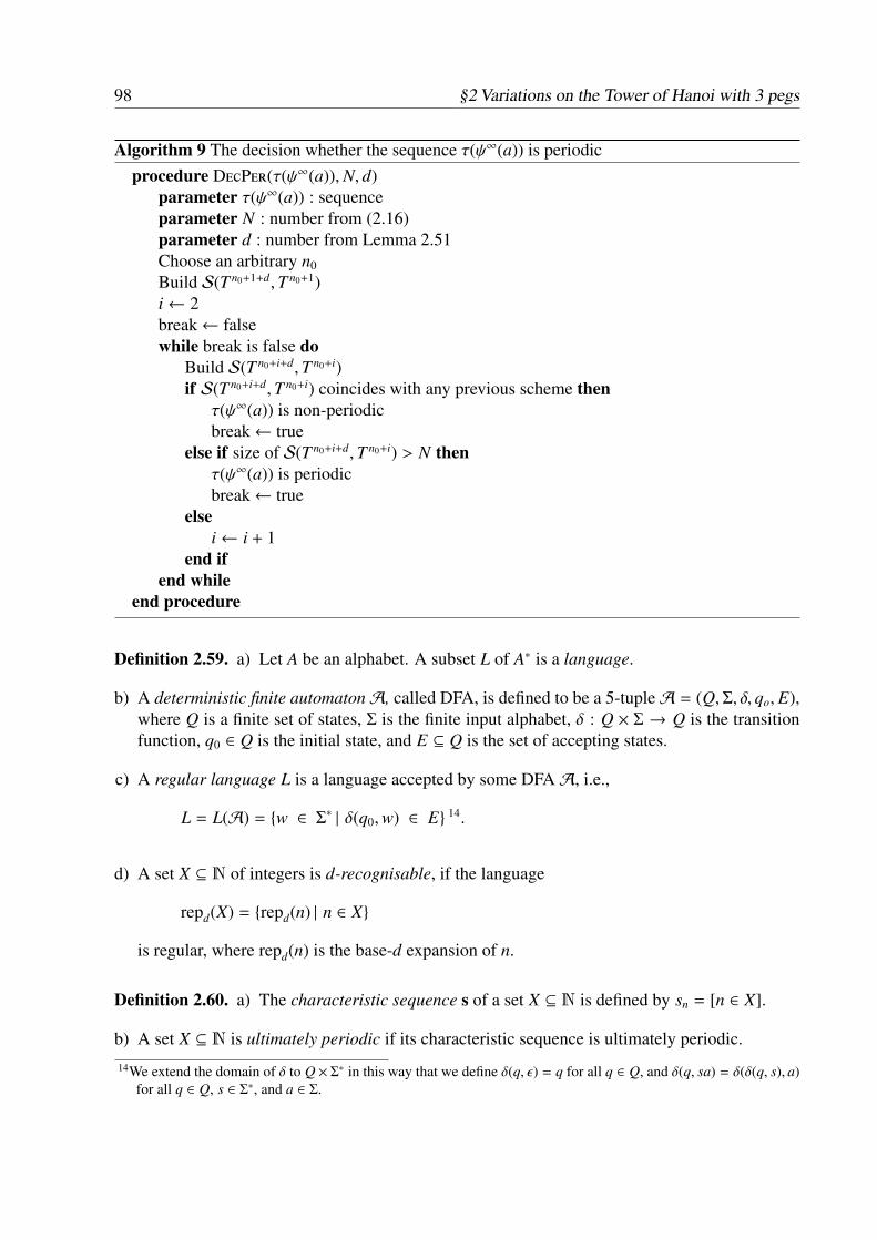
98 §2 Variations on the Tower of Hanoi with 3 pegs
Algorithm 9 The decision whether the sequence τ(ψ∞(a)) is periodicprocedure DecPer(τ(ψ∞(a)),N, d)
parameter τ(ψ∞(a)) : sequenceparameter N : number from (2.16)parameter d : number from Lemma 2.51Choose an arbitrary n0
Build S(T n0+1+d,T n0+1)i← 2break← falsewhile break is false do
Build S(T n0+i+d,T n0+i)if S(T n0+i+d,T n0+i) coincides with any previous scheme then
τ(ψ∞(a)) is non-periodicbreak← true
else if size of S(T n0+i+d,T n0+i) > N thenτ(ψ∞(a)) is periodicbreak← true
elsei← i + 1
end ifend while
end procedure
Definition 2.59. a) Let A be an alphabet. A subset L of A∗ is a language.
b) A deterministic finite automatonA, called DFA, is defined to be a 5-tupleA = (Q,Σ, δ, qo, E),where Q is a finite set of states, Σ is the finite input alphabet, δ : Q × Σ → Q is the transitionfunction, q0 ∈ Q is the initial state, and E ⊆ Q is the set of accepting states.
c) A regular language L is a language accepted by some DFAA, i.e.,
L = L(A) = {w ∈ Σ∗ | δ(q0,w) ∈ E} 14.
d) A set X ⊆ N of integers is d-recognisable, if the language
repd(X) = {repd(n) | n ∈ X}
is regular, where repd(n) is the base-d expansion of n.
Definition 2.60. a) The characteristic sequence s of a set X ⊆ N is defined by sn = [n ∈ X].
b) A set X ⊆ N is ultimately periodic if its characteristic sequence is ultimately periodic.14We extend the domain of δ to Q × Σ∗ in this way that we define δ(q, ε) = q for all q ∈ Q, and δ(q, sa) = δ(δ(q, s), a)
for all q ∈ Q, s ∈ Σ∗, and a ∈ Σ.

§2 Variations on the Tower of Hanoi with 3 pegs 99
A connection between the d-recognisable sets and the d-automatic sequences is given by the sub-sequent lemma.
Lemma 2.61 ([69, Proposition 1.37]). Let d ∈ N2. A set X ⊆ N is d-recognisable if and only if itscharacteristic sequence is d-automatic.
Example 2.62. A well-known example of a 2-recognisable set is the Prouhet-Thue-Morse set
{n ∈ N | rep2(n) contains an odd number of 1s}.
Its characteristic sequence is the Prouhet-Thue-Morse sequence
t = 0110100110010110 . . . .
According to Examples 2.3 and 2.4, the Prouhet-Thue-Morse sequence is 2-automatic. One canfind more details concerning this sequence in [1].
We make use of the following proposition to state the theorem about ultimately periodic se-quences.
Proposition 2.63 ([12, Proposition 1.5.3]). Let d ∈ N2. Any ultimately periodic set X ⊆ N isd-recognisable.
Remark. We can also formulate Cobham’s Theorem 2.32 in the field of recognisable sets. Let pand q be multiplicatively independent integers and let X ⊆ N be both p- and q-recognisable. ThenX is ultimately periodic.
With the proposition we can now deduce our theorem.
Theorem 2.64. Any ultimately periodic sequence is d-automatic for all d ∈ N2.
An alternative proof of this theorem was given in [8, Theorem 5.4.2].By the decision between periodicity and non-periodicity, we can deduce either the non-automaticityof the sequence u for any d ∈ N2 or the automaticity for all d ∈ N2.
2.4 Conclusion and Outlook
In this chapter we disproved the automaticity of the T H(C+3 ) sequence w. We used a theorem of
Cobham which says that in an automatic sequence the frequency of a letter is rational, if it exists.By showing that the frequencies of all letters exist and are irrational, we could conclude that, forany d, w is not d-automatic. This confirms the Allouche-Sapir Conjecture concerning the T H(C+
3 )sequence.

100 §2 Variations on the Tower of Hanoi with 3 pegs
Since we could not ascertain whether the frequency of a letter in the T H(K−3 ) sequence u is ir-rational, we chose a new approach where we made use of another theorem of Cobham. It saysthat, if one has two multiplicatively independent numbers k and l and a sequence is both k- andl-automatic, then the sequence is ultimately periodic. By disproving the ultimate periodicity, wewould be able to conclude that the sequence is not automatic. For this purpose, we had so fartwo proofs on hand which show the decidability of the question on the ultimate periodicity, oneof F. Durand and one of I. V. Mitrofanov. First, we proved that u is the image, under a coding, ofan iterative fixed point of a primitive prolongable endomorphism. According to Durand, we canthen decide about the ultimate periodicity of this sequence. But it turned out that the necessarycalculations are very complex.For Mitrofanov’s proof we needed the set of generating words and the subword schemes of thesequence. We determined this set and a subword scheme. Hereafter, an algorithm for the decisionabout the periodicity was given. We formulated a sufficient condition for the automaticity of theT H(K−3 ) sequence. But for the final decision about the periodicity a few numbers remained to as-certain. In both approaches, first, one will have to calculate the numbers Rν from Definition 2.44and Qν from Lemma 2.45 with the aid of Algorithm 8. Depending on the method, one will havethen to determine Kν and K of (2.13) to apply Theorem 2.43 or L1, L2, and λ as we saw in this sec-tion to find N and proceed with Algorithm 9. Since the calculations are going to be very complex,as it was already predicted for the general case in [26, Chapter 1.3], one will have to make use ofthe capabilities of high performance computing. But these efforts are worth it, since the proof ofultimate periodicity provides a unique decision whether u is d-automatic or not.

Chapter 3
The Star Tower of Hanoi: a variant of theTower of Hanoi with 4 pegs
In the previous chapter we considered variants of the Hanoi graphs which were directed graphs.Now we take a closer look at directed graphs to specify then a special form of them. Recall that adirected graph (or digraph) with vertex set V and arc set A is a graph in which all arcs are directed.In a digraph the in-degree of a vertex v ∈ V is the number of arcs with v as terminal vertex.Similarly, the out-degree of a vertex v ∈ V is given by the number of arcs which leave the vertex v.Then we define
Definition 3.1. A (directed) star S t(p) depending on p ∈ N is a directed graph with vertex setV = [p]0 and arc set A = {(0, i), (i, 0) : i ∈ [p − 1]}.
It is easily seen that every (directed) star has p − 1 vertices with [in-degree, out-degree] = [1, 1]and one vertex, namely the center, with [p−1, p−1]. A (directed) star is, of course, also a simple,undirected graph. This structure can be used to find new variants of the Tower of Hanoi. Thenumber p stands here for the p pegs, where the vertex 0 or peg 0 is always the central peg. One ofthe simplest examples for these variants is the Linear TH, here called the T H(S t(3)), on three pegs,which we already know from the previous chapter. The version with four pegs, namely T H(S t(4)),is of special interest, since it is similar to the unrestricted The Reve’s puzzle.In 1994, Paul K. Stockmeyer introduced in [78] this new variant. According to the underlyingdirected star S t(4) on four pegs, it consists of three pegs, labeled 1, 2, and 3, arranged in anequilateral triangle, and one peg, labeled 0, in the center. The only allowed moves are between thecentral peg and the external ones. The move from 0 to 1 is called a and in the opposite direction a,b goes from 0 to 2 and b back and c goes from 0 to 3 and c back (see Figure 3.1). We will shortlysee why we chose this labelling.In the book [33] we can find this puzzle as well. Both sources looked at the problem to transfera perfect tower from an external peg to another external peg. They determined the minimumnumber of moves for this question among the algorithms which apply the Frame-Stewart-typestrategy. The Frame-Stewart-type strategy is based on the two different algorithms to solve the
101

102 §3 The Star Tower of Hanoi: a variant of the Tower of Hanoi with 4 pegs
The Reve’s puzzle by B. M. Stewart and J. S. Frame. For the The Reve’s puzzle, it turned out thatthe presumed minimum numbers of moves arising from the respective algorithms are the samefor both strategies ([33, Proposition 5.3]). The same was shown for n ∈ N and p ∈ N3, i.e.,for the Multi-Peg Tower of Hanoi, in [53]. Hence we call it the Frame-Stewart-type strategy. Inthe editorial note by O. Dunkel to [76], it was pointed out that the proof that these algorithmsare optimal was still lacking. This problem was known in the literature as the Frame-StewartConjecture.
b
b
b
b
2 0 31
a a
b
b c
c
1
Figure 3.1: The directed star S t(4) on four pegs
We come back to our puzzle. To analyse the solution, use was made of the already known optimalalgorithms for the Linear TH on three pegs in [33, Chapter 8.3]. We chose the above labellingof the moves in the Star TH in view of the similarity to the Linear TH, for instance if we omitpeg 3 and the corresponding moves. The algorithm to solve the Star TH problem with n discs forthe case “external peg to another external peg” is described in the sequel. To this end, let n ∈ N,m ∈ [n] and k ∈ [3].
1. Recursively move the smallest n − m discs from the source peg to the non-goal peg k;
2. Avoiding peg k, move the largest m discs from the source peg to the goal peg;
3. Recursively move the smallest n − m discs from peg k to the goal peg.
If n = 0, we fix m = 0. Obviously, the second part is solved by the same algorithm as theLinear TH, where we want to move the discs from the non-central peg to the other non-centralpeg. In [33, Chapter 8], this algorithm is called Linear-02(m). Algorithm 10, as well as the lateralgorithm for the Linear TH, arises from the application of The Sapir Algorithm 7 in Chapter 2 onthe digraph of the Linear TH.
We know by [33, Section 8.1] and [78, Section 3] that we need 3m−1 moves to transfer the perfecttower in the Linear TH with Linear-02(m). Hence, we set for the Star TH
S t012 = 0; ∀n ∈ N : S tn
12 = min{2S tn−m
12 + 3m − 1 | m ∈ [n]}
(3.1)

§3 The Star Tower of Hanoi: a variant of the Tower of Hanoi with 4 pegs 103
Algorithm 10 Linear: from the non-central peg to the other non-central pegprocedure Linear-02(n)
parameter n : number of discs {n ∈ N0}
if n , 0 thentransfer n − 1 smallest discs from the non-central source peg to non-central goal pegmove disc n from non-central source peg to central pegtransfer n − 1 smallest discs from non-central goal peg to non-central source pegmove disc n from central peg to non-central goal pegtransfer n − 1 smallest discs from non-central source peg to non-central goal peg
end ifend procedure
For abbreviation, we wrote S tn instead of S tn(4). For n = 1, 2 we calculate that m = 1 is optimal,but for n = 3, 4, 5 and 6 we get m = 2 and finally m = 3 or more for n ≥ 7 . In the next theoremwe specify this in general.
Theorem 3.2 ([78, Theorem 2], [33, Theorem 8.8]). The value
m =
⌊ln(a(3)
n )ln(3)
⌋+ 1,
where a(3)n is n-th element of the 3-smooth sequence15, is the unique value that defines S tn
12 in (3.1).In the resulting algorithm, for every i ∈ [n], there is a disc which makes exactly 2a(3)
i moves, i.e.,altogether
S tn12 = 2
n∑i=1
a(3)i
for the minimum number of moves using the Frame-Stewart-type strategy.
This method followed the lines of B. M. Stewart. But there is another possible approach. We canlook at the halfway situation before the only move of the largest disc as well. This procedure isdue to J. S. Frame. If we try to apply Frame’s idea, we would get a new algorithm with n ∈ N,m ∈ [n]0 and k ∈ [3] :
1. Move the smallest n − m − 1 discs from the source peg to the non-goal k;
2. Avoiding peg k, move m discs from the source peg to the goal peg;
3. Move the largest disc from the source peg to the central peg;
4. Avoiding peg k, move m discs from the goal peg to the source peg;
15The 3-smooth sequence(a(3)
n
)n∈N
consists of the 3-smooth numbers 2 j · 3k, j, k ∈ N0 ordered increasingly:a(3) = (1, 2, 3, 4, 6, 8, 9, 12, 16, 18, 24, 27 . . .)

104 §3 The Star Tower of Hanoi: a variant of the Tower of Hanoi with 4 pegs
5. Move the largest disc from the central peg to the goal peg;
6. Avoiding peg k, move m discs from the source peg to the goal peg;
7. Move the smallest n − m − 1 discs from peg k to the goal peg.
For n = 0 we set m = 0 and use only the third and the fifth step. But this does not really followFrame as we have two moves of the largest disc. Here, it is not possible to move the largest discin one move from the source peg to the (non-central) goal peg. Indeed, only Stewart’s approach isapplicable, as we already stated in Theorem 3.2.
But what happens if it is our aim to transfer the perfect tower with n ∈ N discs from the centralpeg 0 to an external peg or in the opposite direction? First, we use Stewart’s approach. Let n ∈ N,m ∈ [n] and again k ∈ [3]. Then this algorithm solves the problem 0n → 1n/2n/3n :
1. Recursively move the smallest n − m discs from the central peg 0 to a non-goal peg k;
2. Avoiding peg k, move the m largest discs from central peg 0 to the goal peg;
3. Recursively move the smallest n − m discs from peg k to the goal peg
or in the opposite direction 1n/2n/3n → 0n :
1. Recursively move the smallest n − m discs from the source peg to a non-goal peg k;
2. Avoiding peg k, move the largest m discs from the source peg to the central (goal) peg;
3. Recursively move the smallest n − m discs from peg k to the central (goal) peg.
For the case n = 0 we fix m = 0.
Algorithm 11 Linear: from source peg to central peg or from central peg to goal pegprocedure Linear-01(n)
parameter n : number of discs {n ∈ N0}
if n , 0 thentransfer n − 1 smallest discs from source peg to non-central, non-goal pegmove disc n from source peg to goal pegtransfer n − 1 smallest discs from non-central, non-goal peg to goal peg
end ifend procedure
The second part of both is solved by the algorithm Linear-01(m), which needs 12 (3m − 1) moves,
since every disc d ∈ [n] \ [n − m] moves 3n−d times in the solution.

§3 The Star Tower of Hanoi: a variant of the Tower of Hanoi with 4 pegs 105
Being interested in the minimum number of moves for the “central peg to external peg” problem,we set
S t001 = 0; ∀n ∈ N : S tn
01 = min
S tn−m01 +
12
(3m − 1) + S tn−m12︸︷︷︸
=2∑n−m
i=1 a(3)i
| m ∈ [n]
. (3.2)
Again, we can calculate the first few values of m. We see that
m = 1 for n = 1, 2m = 2 for n = 3, 4, 5m = 3 for n = 5, 6, 7, 8, 9m ≥ 4 for n = 10, 11, 12, . . . .
It is conspicuous that we have two options for n = 5. Now we are able to find the sequences ofdisc moves for the first first few values of n, as it is done in Tables 3.1 and 3.2. It will turn outthat for n = 5, 8 and 12 we have two different sequences of disc moves whereby the total numberof moves are equal for both possibilities. This phenomenon will presumably occur for greater nagain and again, since it arises from the recursive structure of the calculation of the total numberof moves with Formula (3.2).
We can also summarise the total number of moves for the first values of n in a sequence:
S t01 = (1, 4, 7, 14, 23, 32, 47, 68, 93, 120, 153, 198, . . .) (3.3)
Further elements of this sequence can be found again by Formula (3.2) and the comparison of thetotal number of moves for different m. Here, too, we can make use of the recursive structure of thecalculations in Tables 3.1 and 3.2.
After rewriting the expression S tn01 the number is equal to S tn
10, which is the recursion for theminimum number of moves for the “external peg to central peg” problem, since
S tn01 = min
{S tm′
01 +12
(3n−m′ − 1
)+ S tm′
12 | m′ ∈ [n]0
}and
S tn10 = min
{S tm′
12 +12
(3n−m′ − 1
)+ S tm′
10 | m′ ∈ [n]0
}.
Now we have to look at Frame’s approach and the questions whether it is applicable in this caseand if there is a difference to the number of moves resulting from Stewart’s way. First, we find thealgorithms for the two directions and see that the largest disc moves only once. Correspondingto the above recursions, we call the recursion for the presumed minimum number of moves usingFrame S tn+1
01 and S tn+110 .

106 §3 The Star Tower of Hanoi: a variant of the Tower of Hanoi with 4 pegs
disc d nom disc d nomn=1,m=1: 1 1n=2,m=1: 1 3
2 1n=3,m=2: 1 3
2 33 1
n=4,m=2: 1 72 33 34 1
n=5,m=2: 1 7 m=3: 1 72 9 2 33 3 3 94 3 4 35 1 5 1
n=6,m=3: 1 72 93 34 95 36 1
n=7,m=3: 1 152 73 94 35 96 37 1
n=8,m=3: for n-m=5:m’=2: 1 15 m’=3: 1 15
2 21 2 153 7 3 134 9 4 95 3 5 36 9 6 97 3 7 38 1 8 1
disc d nomn=9,m=3: 1 23
2 173 154 135 96 37 98 39 1
n=10,m=4: 1 232 173 154 135 96 37 278 99 3
10 1n=11,m=4: 1 31
2 153 214 75 276 97 38 279 9
10 311 1
Table 3.1: Calculations of the number of moves (nom) of each disc for n = 1, . . . , 11 for theminimising value m

§3 The Star Tower of Hanoi: a variant of the Tower of Hanoi with 4 pegs 107
disc d nom disc d nomn=12,m=4: for n-m=8:m’=2: 1 31 m’=3: 1 31
2 45 2 393 15 3 214 21 4 215 7 5 76 27 6 277 9 7 98 3 8 39 27 9 2710 9 10 911 3 11 312 1 12 1
Table 3.2: Calculations of the number of moves (nom) of each disc for n = 12 for the minimisingvalue m
Again, let n ∈ N0 and k ∈ [3]. If we go from 0n+1 → 1n+1/2n+1/3n+1 , we use the followingalgorithm with m′ ∈ [n + 1]0 and k′ ∈ [3] \ {k} :
1. Move m′ discs from the central peg to the non-goal peg k;
2. Avoiding peg k, move n − m′ discs from the central peg to the non-goal peg k′;
3. Move the largest disc from the central to the goal peg;
4. Avoiding peg k, move n − m′ discs from the non-goal peg k′ to the goal peg;
5. Move m′ discs from peg k to the goal peg
Fo the case that we want to go from 1n+1/2n+1/3n+1 → 0n+1, we apply this algorithm, again withm′ ∈ [n + 1]0 and k′ ∈ [3] \ {k} :
1. Move m′ discs from the source peg to the non-goal, non-central peg k;
2. Avoiding peg k, move n − m′ discs from the source peg to the non-goal peg k′;
3. Move the largest disc from the source peg to the central peg;
4. Avoiding peg k, move n − m′ discs from peg k′ to the central peg;
5. Move m′ discs from peg k to the central peg.

108 §3 The Star Tower of Hanoi: a variant of the Tower of Hanoi with 4 pegs
We simplify the formulas of S tn+101 and S tn+1
10 to compare them with the numbers S tn+101 and S tn+1
10 .
S tn+101 = min
{S tm′
01 +12
(3n−m′+1 − 1
)+ S tm′
12 | m′ ∈ [n + 1]0
}S tn+1
10 = min{
S tm′12 +
12
(3n−m′+1 − 1
)+ S tm′
10 | m′ ∈ [n + 1]0
}.
The corresponding numbers in Frame’s version are
S tn+101 = min
{S tm′
01 +12
(3n−m′ − 1
)+ 1 +
(3n−m′ − 1
)+ S tm′
12 | m′ ∈ [n + 1]0
}= min
{S tm′
01 +12
(3n−m′+1 − 1
)+ S tm′
12 | m′ ∈ [n + 1]0
}and
S tn+110 = min
{S tm′
12 +(3n−m′ − 1
)+ 1 +
12
(3n−m′ − 1
)+ S tm′
10 | m′ ∈ [n + 1]0
}= min
{S tm′
12 +12
(3n−m′+1 − 1
)+ S tm′
10 | m′ ∈ [n + 1]0
}.
By comparing the numbers, we obtain that the respective recursions for Stewart’s and Frame’sstrategy coincide. We conclude that it is enough to look at Stewart’s version for all transfers of aperfect tower from the central peg to an arbitrary external peg in the Star TH. Hence we can alsouse the common term Frame-Stewart-type strategy.
The question whether the Frame-Stewart-type strategy is optimal for the problems to transfer aperfect tower from an external peg to another external peg or from the central peg to an arbitraryexternal peg is still open. One very helpful step could be the proof the Frame-Stewart Conjecturefor four pegs, which was found by T. Bousch [13] in 2014. Stockmeyer [79] has already doneexhaustive computer searches on the “external peg to external peg” problem and the “central pegto external peg” problem in the Star TH with four pegs. For the first problem, he got for the totalrequired number of moves
2, 6, 12, 20, 32, 48, 66, 90, 122, 158, 206, 260, 324, 396, 492, and 600 for n = 1, 2, . . . , 16.
These are exactly the values of S tn12 in Theorem 3.2 for n = 1, . . . , 16. For the second problem, he
calculated
1, 4, 7, 14, 23, 32, 47, 68, 93, 120, 153, 198, 255, 318, and 399 for n = 1, 2, . . . , 15.
The beginning of this sequence corresponds to the sequence of (3.3), which we calculated hereusing the Frame-Stewart-type strategy. With the aid of the OEIS (The on-line encyclopedia ofinteger sequences) and by generating more data, one could probably find a system in the sequenceof numbers for which we have two different sequences of disc moves or for which we have two

§3 The Star Tower of Hanoi: a variant of the Tower of Hanoi with 4 pegs 109
different possible ms (For instance, the phenomenon of n = 5 occurs again at n = 8, 12, 15). Butthe main interest beside these sequences is to search for a regularity in the sequence of ms forthe presumed minimal number of moves S tn
01, as it was found for the sequence of values m forthe presumed minimal number of moves S tn
12 in the use of the 3-smooth sequence(a(3)
n
)n∈N
(OEISA003586) by Stockmeyer.Obviously, this puzzle can be extended to p ∈ N3 by considering the directed star S t(p). We applyagain the Frame-Stewart-type strategy on the “external peg to external peg” problem and get asalgorithm for n ∈ N, m ∈ [n], and k ∈ [p − 1]:
1) Recursively move the smallest n − m discs from the source peg to the non-goal peg k,
2) Avoiding peg k, move the largest m discs from the source peg to the goal peg,
3) Recursively move the smallest n − m discs from peg k to the goal peg.
If n = 0, we set m = 0. The first and the third step must be solved in the Star TH with p pegsfor the “external peg to external peg” problem, whereas the second one in the Star TH with only(p − 1) pegs. Stockmeyer [79] found out that for a very large number of discs for k ∈ N thereare
(k+p−5
p−4
)=
(k+p−5
k−1
)discs that each make exactly 2k · 3 j moves for all j ∈ N0. Considering the
“central peg to external peg” problem, we get as algorithm for n ∈ N, m ∈ [n], and k ∈ [p − 1]:
1) Recursively move the smallest n − m discs from the central peg to the non-goal peg k,
2) Avoiding peg k, move the largest m discs from the central peg to the goal peg,
3) Recursively move the smallest n − m discs from peg k to the goal peg.
Again, if n = 0, we fix m = 0. Here we have twice the Star TH with p pegs for the “central peg toexternal peg” problem or the “external peg to external peg” problem, respectively, and once with(p − 1) pegs for the “central peg to external peg” problem. For a further analysis one could lookagain at Frame and his approach in [76]. But it would turn out that his induction proof is herenot applicable as we do not know enough about the Star TH for the “external peg to external peg”problem yet. The problem for p pegs requires further research. One aim would be to find theminimum number of moves or at least a similar statement for the disc moves as for the “externalpeg to external peg” problem.


Bibliography
[1] J.-P. Allouche and J. Shallit. The Ubiquitous Prouhet-Thue-Morse Sequence. In: C. Ding,T. Helleseth, and H. Niederreiter (eds.), Sequences and their Applications, Discrete Math-ematics and Theoretical Computer Science, pages 1–16. Springer, London, 1999.
[2] J.-P. Allouche. Note on the cyclic towers of Hanoi. Theoretical Computer Science, 123(1):3–7, 1994.
[3] J.-P. Allouche. private communication, 2015.
[4] J.-P. Allouche, J. Bétréma, and J. Shallit. Sur des points fixes de morphismes d’un monoïdelibre. RAIRO - Informatique Théorique et Applications, 23(3):235–249, 1989.
[5] J.-P. Allouche and F. Dress. Tours de Hanoï et automates. RAIRO - Informatique Théoriqueet Applications, 24(1):1–15, 1990.
[6] J.-P. Allouche, N. Rampersad, and J. Shallit. Periodicity, Repetitions, and Orbits of anAutomatic Sequence. Theoretical Computer Science, 410(30):2795–2803, 2009.
[7] J.-P. Allouche and A. Sapir. Restricted towers of Hanoi and morphisms. In: C. de Feliceand A. Restivo (eds.), Proceedings of the Ninth International Conference of Developmentsin Language Theory (DLT’05), LNCS 3572, pages 1–10, 2005.
[8] J.-P. Allouche and J. O. Shallit. Automatic Sequences - Theory, Applications, Generaliza-tions. Cambridge University Press, Cambridge, 2003.
[9] M. D. Atkinson. The Cyclic Towers of Hanoi. Information Processing Letters, 13(3):118–119, 1981.
[10] D. Azriel, N. Solomon, and S. Solomon. On an Infinite Family of Solvable Hanoi Graphs.ACM Transactions on Algorithms, 5(1), 2008. Article no. 13.
[11] W. W. R. Ball. Mathematical recreations and essays. Macmillan and Co., Limited, London,6th edition, 1914.
[12] V. Berthé and M. Rigo (eds.). Combinatorics, Automata and Number Theory. Cambridge
111

112 Bibliography
University Press, Cambridge, 2010.
[13] T. Bousch. La quatrième tour de Hanoï. Bulletin of the Belgian Mathematical Society -Simon Stevin, 21:895–912, 2014.
[14] J. Cassaigne and F. Nicolas. Quelques propriétés de mots substitutifs. Bulletin of the BelgianMathematical Society - Simon Stevin, 10(5):661–677, 2003.
[15] J. Chappelon and A. Matsuura. On generalized Frame-Stewart numbers. Discrete Mathem-atics, 312(5):830–836, 2012.
[16] É. Charlier, J. Leroy, and M. Rigo. Asymptotic properties of free monoid morphisms. LinearAlgebra and its Applications, 500:119–148, 2016.
[17] A. Cobham. On the Base-Dependence of Sets of Numbers Recognizable by Finite Automata.Mathematical Systems Theory, 3(2):186–192, 1969.
[18] A. Cobham. Uniform Tag Sequences. Mathematical Systems Theory, 6(1):164–192, 1972.
[19] R. Cooke. Classical Algebra: Its Nature, Origins, and Uses. Wiley, Hoboken, NJ, 2008.
[20] L. L. Cristea and B. Steinsky. Distances in Sierpinski graphs and on the Sierpinski gasket.Aequationes Mathematicae, 85(3):201–219, 2013.
[21] D. Damanik and D. Lenz. Substitution dynamical systems: Characterization of linear repet-itivity and applications. Journal Mathematical Analysis and Applications, 321(2):766–780,2006.
[22] H. de Parville. Récréations mathématiques: La tour d’Hanoï et la question du tonkin. LaNature, 12:285–286, 1884.
[23] H. E. Dudeney. The Canterbury puzzles and other curious problems. E. P. Dutton and Co.,New York NY, 1908.
[24] F. Durand. A characterization of substitutive sequences using return words. Discrete Math-ematics, 179:89–101, 1998.
[25] F. Durand. HD0L ω-equivalence and periodicity problems in the primitive case (to thememory of G. Rauzy). Journal of Uniform Distribution Theory, 7(1):199–215, 2012.
[26] F. Durand. Decidability of the HD0L ultimate periodicity problem. RAIRO - TheoreticalInformatics and Applications, 47(2):201–214, 2013.
[27] F. Durand. Decidability of uniform recurrence of morphic sequences. International Journalof Foundations of Computer Science, 24(1):123–146, 2013.
[28] F. Durand, B. Host, and C. Skau. Substitution dynamical systems, Bratteli diagrams and

Bibliography 113
dimension groups. Ergodic theory and Dynamical Systems, 19:953–993, 1999.
[29] M. Eie and S.-T. Chang. A Course on Abstract Algebra. World Scientific Publishing Com-pany, Singapore, 2010.
[30] F. Harary and E. M. Palmer. Graphical Enumeration. Academic Press, New York NY, 1973.
[31] T. Harju and M. Linna. On the periodicity of morphisms on free monoids. RAIRO - Inform-atique Théorique et Applications, 20(1):47–54, 1986.
[32] H. Hering. Genetische Mathematisierung am Beispiel einer Variante des Turm-von-Hanoi-Spiels. Didaktik der Mathematik, 4:307–317, 1978.
[33] A. M. Hinz, S. Klavžar, U. Milutinovic, and C. Petr. The Tower of Hanoi—Myths and Maths.Birkhäuser, Basel, 2013.
[34] A. M. Hinz. The Tower of Hanoi. L’Enseignement Mathématique (2), 35:289–321, 1989.
[35] A. M. Hinz. Square-free Tower of Hanoi sequences. L’Enseignement Mathématique (2),42:257–264, 1996.
[36] A. M. Hinz. private communication, 2016.
[37] A. M. Hinz and C. H. auf der Heide. An efficient algorithm to determine all shortest paths inSierpinski graphs. Discrete Applied Mathematics, 177:111–120, 2014.
[38] A. M. Hinz, S. Klavžar, U. Milutinovic, D. Parisse, and C. Petr. Metric properties of theTower of Hanoi graphs and Stern’s diatomic sequence. European Journal of Combinatorics,26(5):693–708, 2005.
[39] A. M. Hinz, S. Klavžar, and S. S. Zemljic. Sierpinski graphs as spanning subgraphs of Hanoigraphs. Central European Journal of Mathematics, 11(6):1153–1157, 2013.
[40] A. M. Hinz, S. Klavžar, and S. S. Zemljic. A survey and classification of Sierpinski-typegraphs. Discrete Applied Mathematics, 2016. to appear.
[41] A. M. Hinz and D. Parisse. The Average Eccentricity of Sierpinski Graphs. Graphs andCombinatorics, 28(5):671–686, 2012.
[42] A. M. Hinz and A. Schief. The average distance on the Sierpiniski gasket. Probability Theoryand Related Fields, 87:129–138, 1990.
[43] A. M. Hinz and S. S. Zemljic. Sierpinski triangle graphs. submitted, 2016.
[44] HLRB Project pr87mo: ToHdiameter. URL: https://www.lrz.de/projekte/hlrb-projects/0000000000F437A5.html. last visited on 08/08/2016.

114 Bibliography
[45] J. Honkala. A decision method for the recognizability of sets defined by number systems.RAIRO - Informatique Théorique et Applications, 20(4):395–403, 1986.
[46] J. Honkala. On the simplification of infinite morphic words. Theoretical Computer Science,410(8):997–1000, 2009.
[47] J. Honkala and M. Rigo. Decidability questions related to abstract numeration systems.Discrete Mathematics, 285:329–333, 2004.
[48] R. A. Horn and C. R. Johnson. Matrix Analysis. Cambridge University Press, Cambridge,2nd edition, 2013.
[49] T. W. Hungerford. Algebra. Springer, New York, 1974.
[50] M. Jakovac. A 2-parametric generalization of Sierpinski gasket graphs. Ars Combinatoria,116:395–405, 2014.
[51] A. Kanel-Belov and I. V. Mitrofanov. Periodicity of Rauzy Scheme and Substitutional Sys-tems. arXiv:1107.0185 [math.DS], 2012.
[52] S. Klavžar and U. Milutinovic. Graphs S (n, k) and a variant of the Tower of Hanoi problem.Czechoslovak Mathematical Journal, 47(1):95–104, 1997.
[53] S. Klavžar, U. Milutinovic, and C. Petr. On the Frame-Stewart algorithm for the multi-pegTower of Hanoi problem. Discrete Applied Mathematics, 120:141–157, 2002.
[54] S. Klavžar and S. S. Zemljic. On distances in Sierpinski graphs: Almost-extreme verticesand metric dimension. Applicable Analysis and Discrete Mathematics, 7:72–82, 2013.
[55] R. E. Korf. Best-First Frontier Search with Delayed Duplicate Detection. In: NineteenthNational Conference on Artificial Intelligence (AAAI-2004), The MIT Press, CambridgeMA, pages 650–657, 2004.
[56] R. E. Korf and A. Felner. Recent Progress in Heuristic Search: A Case Study of the Four-PegTowers of Hanoi Problem. In: M. M. Veloso (ed.), Proceedings of the Twentieth Interna-tional Joint Conference on Artificial Intelligence (IJCAI-07), AAAI Press, Menlo Park CA,pages 2324–2329, 2007.
[57] E. Leiss. Solving the “Towers of Hanoi” on Graphs. Journal of Combinatorics, Informationand System Sciences, 9(1):81–89, 1983.
[58] E. Leiss. The worst Hanoi graphs. Theoretical Computer Science, 498:100–106, 2013.
[59] D. Lind and B. Marcus. An Introduction to Symbolic Dynamics and Coding. CambridgeUniversity Press, Cambridge, 1995.
[60] É. Lucas. Récréations mathématiques. Gauthier-Villars et fils, Paris, 1882–1894. 4 volumes.

Bibliography 115
[61] P. Michel. Stricte ergodicité d’ensembles minimaux de substitution. In: J.-P. Conze andM. S. Keane (eds.), Théorie Ergodique: Actes des Journées Ergodiques, Rennes 1973/1974,LNCS 532, pages 189–201, 1976.
[62] I. V. Mitrofanov. A Proof for the Decidability of HD0L Ultimate Periodicity.arXiv:1110.4780, 2012.
[63] I. V. Mitrofanov. Periodicity of Morphic Words. Journal of Mathematical Sciences,206(6):679–687, 2015.
[64] F. Nicolas and Y. Pritykin. On uniformly recurrent morphic words. International Journal ofFoundations of Computer Science, 20(5):919–940, 2009.
[65] J.-J. Pansiot. Hiérarchie et fermeture de certaines classes de tag-systèmes. Acta Informatica,20(2):179–196, 1983.
[66] J.-J. Pansiot. Complexité des Facteurs des Mots Infinis Engendrés par Morphismes Itérés.In: J. Paredaens (ed.), Automata, Languages and Programming, LNCS 172, pages 380–389,1984.
[67] J.-J. Pansiot. Decidability of periodicity for infinite words. RAIRO - Informatique Théoriqueet Applications, 20(1):43–46, 1986.
[68] D. Parisse. On some metric properties of the Sierpinski graphs S (n, k). Ars Combinatoria,90:145–160, 2009.
[69] M. Rigo. Formal Languages, Automata and Numeration systems, volume 2. ISTE Ltd. andJohn Wiley & Sons Inc., London and Hoboken, 2014.
[70] D. Romik. Shortest Paths in the Tower of Hanoi Graph and Finite Automata. SIAM Journalon Discrete Mathematics, 20(3):610–622, 2006.
[71] K. Saari. On the frequency of letters in pure binary morphic sequences. In: C. de Feliceand A. Restivo (eds.), Proceedings of the Ninth International Conference of Developmentsin Language Theory (DLT’05), LNCS 3572, pages 397–408, 2005.
[72] K. Saari. On the Frequency of Letters in Morphic Sequences. In: D. Grigoriev, J. Harrison,and E. A. Hirsch (eds.), Computer Science - Theory and Applications, LNCS 3967, pages334–345, 2006.
[73] A. Salomaa and M. Soittola. Automata-Theoretic Aspects of Formal Power Series. Springer,1978.
[74] A. Sapir. The Tower of Hanoi with Forbidden Moves. The Computer Journal, 47(1):20–24,2004.
[75] R. S. Scorer, P. M. Grundy, and C. A. B. Smith. Some Binary Games. The Mathematical

116 Bibliography
Gazette, 28(280):96–103, 1944.
[76] B. M. Stewart and J. S. Frame. 3918. The American Mathematical Monthly, 48(3):216–219,1941.
[77] D. Stirzaker. Stochastic processes and models. Oxford University Press, 2005. reprinted2006.
[78] P. K. Stockmeyer. Variations on the Four-Post Tower of Hanoi Puzzle. Congressus Numer-antium, 102:3–12, 1994.
[79] P. K. Stockmeyer. private communication, 2014.
[80] H. Wielandt. Unzerlegbare, nicht negative Matrizen. Mathematische Zeitschrift, 52(1):642–648, 1950.
[81] D. Wood. The towers of Brahma and Hanoi revisited. Journal of Recreational Mathematics,14:17–24, 1981/82.
[82] B. Xue, L. Zuo, G. Wang, and G. Li. Shortest paths in Sierpinski graphs. Discrete AppliedMathematics, 162:314–321, 2014.
Eidesstattliche Erklärung(Siehe Promotionsordnung vom 12.07.11, § 8, Abs. 2 Pkt. .5.)
Hiermit erkläre ich an Eidesstatt, dass die Dissertation von mir selbstständig, ohne unerlaubteBeihilfe angefertigt ist.
Holz auf der Heide, Caroline
Name, Vorname
. . . . . . . . . . . . . . . . . . . . . . . . . .Ort, Datum
. . . . . . . . . . . . . . . . . . . . . . . . . . . . . . . . . . . . . . . . . . .Unterschrift Doktorand/in