Dissipative Energization of Baroclinic Waves by Surface

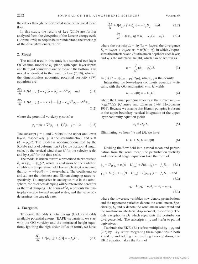
Dissipative Energization of Baroclinic Waves by Surface Ekman Pumping

SUKYOUNG LEE

Department of Meteorology, The Pennsylvania State University, University Park, Pennsylvania

(Manuscript received 24 August 2009, in final form 25 February 2010)

ABSTRACT

A two-layer quasigeostrophic model is used to study the effect of lower boundary Ekman pumping on the

energetics of baroclinic waves. Although the direct impact of the Ekman pumping is to damp the total eddy

energy, either the eddy available potential energy (EAPE) or the eddy kinetic energy (EKE), individually,

can grow because of the Ekman pumping. Growth of EAPE is favored if the phase difference between the

upper and lower wave fields is less than a quarter wavelength, and EKE is favored if the phase difference is

greater than a quarter wavelength. A numerical model calculation shows that the EAPE growth occurs di-

rectly through the Ekman pumping and that the increased EAPE can in turn lead to further growth by

strengthening the baroclinic energy conversion from zonal available potential energy to the EAPE. Through

this indirect effect, the Ekman pumping can increase the net production of total eddy energy.

1. Introduction

In the context of the two-layer quasigeostrophic (QG)

model, it has been known for almost five decades that

Ekman pumping, if present only at the lower bound-

ary, can destabilize baroclinic waves. For example,

Holopainen (1961) performed a linear stability analysis of

the two-layer model and found that the lower boundary

Ekman pumping broadens the marginally stable curve

of the inviscid flow so as to destabilize both longer and

shorter zonal waves. Essentially the same result was

found by Pedlosky (1983), and also by Weng and Barcilon

(1991), who used a linear Eady-like model (Eady 1949).

Pedlosky (1983) further showed, with a weakly nonlinear

analysis, that while the destabilized wave can grow ini-

tially, as the wave changes the mean flow the wave even-

tually decays. The final result is zero wave amplitude with

an altered mean flow.

Nonlinear numerical model calculations also found

that lower-layer Ekman damping can energize baro-

clinic waves. In their study of QG turbulence with a

doubly periodic two-layer model, Hua and Haidvogel

(1986) found that lower-layer Ekman pumping acts as

a source of energy for the baroclinic waves. This finding

was supported by Riviere et al. (2004), who used a prim-

itive equation model to study effect of bottom friction on

baroclinic eddies in an oceanic jet. Using a two-layer QG

model, Lee (2010) showed that surface Ekman pumping

acting directly on the eddies can increase eddy potential

enstrophy. Thompson and Young (2007) found that for b

less than a critical value, the addition of bottom friction

produces a heat flux that is weaker than the inviscid

prediction by Held and Larichev (1996) and Lapeyre and

Held (2003). However, for b larger than a critical value,

the inclusion of bottom friction results in a heat flux that

is stronger than the inviscid prediction. Although linear

destabilization may be relevant for these nonlinear results,

to distinguish between linear and nonlinear influences

the nonlinear behavior will be referred to as ‘‘dissipative

energization’’ and the linear instability as ‘‘dissipative

destabilization.’’

The above nonlinear results suggest for the atmosphere

that surface Ekman pumping may play a nontrivial role for

the equilibration process of midlatitude baroclinic waves.

In spite of the potentially important role of surface Ekman

pumping, the physical process by which Ekman pumping

can energize baroclinic waves is not well understood. Dis-

sipative energization of baroclinic waves, found in various

numerical models, has often been attributed to the baro-

tropic governor mechanism (James and Gray 1986; James

1987). While this may indeed be the case, the mechanism

to be presented in this study differs from the barotropic

governor mechanism, for which surface friction influences

Corresponding author address: Sukyoung Lee, Department of

Meteorology, The Pennsylvania State University, University Park,

PA 16802.

E-mail: [email protected]

JULY 2010 L E E 2251

DOI: 10.1175/2010JAS3295.1

� 2010 American Meteorological SocietyUnauthenticated | Downloaded 10/08/21 09:22 AM UTC

the eddies through the horizontal shear of the zonal mean

flow.

In this study, the results of Lee (2010) are further

analyzed from the viewpoint of the Lorenz energy cycle

(Lorenz 1955) to help us better understand the workings

of the dissipative energization.

2. Model

The model used in this study is a standard two-layer

QG channel model on a b plane, with equal layer depths

and flat rigid boundaries on the top and the bottom. This

model is identical to that used by Lee (2010), wherein

the dimensionless governing potential vorticity (PV)

equations are

›q1

›t1 J(c

1, q

1) 5 k

T(c� c

e)� n=6c

1and (1.1)

›q2

›t1 J(c

2, q

2) 5�k

T(c� c

e)� k

M=2c

2� n=6c

2,

(1.2)

where the potential vorticity qj satisfies

qj5 by 1 =2c

j1 (�1) j

c, j 5 1, 2. (1.3)

The subscript j 5 1 and 2 refers to the upper and lower

layers, respectively, cj is the streamfunction, and c [

(c1 � c2)/2. The model is nondimensionalized by the

Rossby radius of deformation lR for the horizontal length

scale, by the vertical wind shear U for the velocity scale,

and by lR/U for the time scale.

The model is driven toward a prescribed thickness field

ce

[ (ce1� c

e2)/2, which is analogous to the radiative

equilibrium temperature field. For simplicity, it is assumed

that ue2 [ 2›ce2/›y 5 0 everywhere. The coefficients kT

and kM are the thickness and Ekman damping rates, re-

spectively. To emphasize its analogous role in the atmo-

sphere, the thickness damping will be referred to hereafter

as thermal damping. The term n=6cj represents the ens-

trophy cascade toward subgrid scales, and the value of n

determines the cascade rate.

3. Energetics

To derive the eddy kinetic energy (EKE) and eddy

available potential energy (EAPE) separately, we start

with the QG vorticity and the interfacial height equa-

tions. Ignoring the high-order diffusion terms, we have

›z1

›t1 J[c

1, ( f 1 z

1)] 5� f

oD

1, (2.1)

›z2

›t1 J[c

2, ( f 1 z

2)] 5� f

oD

2, and (2.2)

›h

›t1 J(c

2, h) 5 w

I� k

T(h� h

E), (2.3)

where the vorticity zj 5 ›yj /›x 2 ›uj /›y; the divergence

Dj 5 ›uj /›x 1 ›yj /›y; wI 5 w(H 1 h), in which I repre-

sents the interface and H is the mean depth for each layer;

and h is the interfacial height, which can be written as

h 5� f

g*(c

1� c

2)/2. (3)

In (3) g* 5 g[(r2 2 r1)/2r2], where rj is the density.

Integrating the lower-layer continuity equation verti-

cally, with the QG assumption h� H, yields

wI� w(0) 5�D

2H, (4)

where the Ekman pumping velocity at the surface w(0) 5

(kMH/fo)z2 (Charney and Eliassen 1949; Holopainen

1961). Because we assume that Ekman pumping is absent

at the upper boundary, vertical integration of the upper

layer continuity equation yields

wI5 D

1H. (5)

Eliminating wI from (4) and (5), we have

D1H 1 D

2H 5 w(0). (6)

Dividing the flow field into a zonal mean and pertur-

bation from the zonal mean, the perturbation vorticity

and interfacial height equations take the form of

z1t

1 U1z

1x1 y

1(b�U

1yy) 1 J(c

1, z

1) 5� f

oD

1, (7.1)

z2t

1 U2z

2x1 y

2(b�U

2yy) 1 J(c

2, z

2) 5� f

oD

2, and

(7.2)

ht1 U

2h

x1 y

2L

y5 w

1� k

Th,

(7.3)

where the lowercase variables now denote perturbations

and the uppercase variables denote the zonal mean. Spe-

cifically, Uj and L denote the zonal-mean zonal wind and

the zonal-mean interfacial displacement, respectively. The

only exception is Dj, which represents the perturbation

divergence field. The subscripts x, y, and t refer to partial

derivatives.

To obtain the EKE, (7.1) is first multiplied by 2c1 and

(7.2) by 2c2. After integrating these equations in both

x and y, and adding the resulting two equations, the

EKE equation takes the form of

2252 J O U R N A L O F T H E A T M O S P H E R I C S C I E N C E S VOLUME 67

Unauthenticated | Downloaded 10/08/21 09:22 AM UTC

1

2

~$c1

��

��2

1 ~$c2

��

��2

2

0

@

1

A

t

5�1

2�

2

i51U

iy

iz

i1

1

2�

2

i51foD

ic

i(8.1)

5�1

2�

2

i51U

iy

iz

i1 f

o�cD

21

1

2c

1

w(0)

H

" #

(8.2)

5�1

2�

2

i51U

iy

iz

i

|fflfflfflfflfflfflfflfflffl{zfflfflfflfflfflfflfflfflffl}

BT

� focD

2

|fflfflfflfflffl{zfflfflfflfflffl}

C(EAPE,EKE)

11

2k

Mc

1=2c

2

|fflfflfflfflfflfflfflfflfflfflfflffl{zfflfflfflfflfflfflfflfflfflfflfflffl}

EKEEk

, (8.3)

where (6) is used to write (8.2) and the overbar denotes a

zonal average. The first term on the rhs of (8.3), com-

monly referred to as the barotropic conversion (here-

after BT), represents the conversion from zonal kinetic

energy (ZKE) to EKE, and the second term represents

the conversion from EAPE to EKE. The third term

represents the Ekman pumping contribution to the EKE

(hence referred to as EKEEk).

The equation for EAPE can be obtained by multi-

plying (7.3) by g*h/H. Using (3) and (4), the EAPE

equation takes the form of

g*

H

1

2h2

� �

t

5�g*

Hy

2hL

y|fflfflfflfflfflfflffl{zfflfflfflfflfflfflffl}

BC

1 focD

2|fflfflfflfflfflffl{zfflfflfflfflfflffl}

�C(EAPE,EKE)

�kM

c=2c2

|fflfflfflfflfflfflfflffl{zfflfflfflfflfflfflfflffl}

EAPEEk

� kT

g*

Hh2. (9)

The first term on the rhs of (9) is the conversion from

zonal available potential energy (ZAPE) to EAPE, com-

monly known as the baroclinic energy conversion term

(hereafter BC), the second term is the energy conver-

sion from EAPE to EKE, the third term is the Ekman

pumping contribution to the EAPE, and the fourth

term is the radiative damping of EAPE. By adding (8.3)

and (9), the total eddy energy (TEE) equation can be

obtained:

1

2

~$c1

��

��

2

1 ~$c2

��

��

2

21

g*

Hh2

0

BB@

1

CCA

t

5�1

2�

2

i51U

iy

iz

i� g*

Hy

2hL

y�

kM

2~$c

2

��

��

2

|fflfflfflfflfflfflfflfflffl{zfflfflfflfflfflfflfflfflffl}

TEEEk

�kT

g*

Hh2. (10)

The direct contribution of the Ekman damping to the

TEE (TEEEk) is always negative. However, for EKE

and EAPE individually, the Ekman pumping can con-

tribute toward growth. As will be explained shortly, the

latter property is central to the operation of the dissi-

pative energization.

The Ekman pumping can contribute to EKE growth

if the term EKEEk in (8.3) is positive. It can be seen,

after integrating by parts, that EKEEk is positive if~$c1 �~$c2 , 0. If the horizontal scales of c1 and c2 are

equal, this inequality holds if c1 and c2 are negatively

correlated, which corresponds to a phase difference be-

tween c1 and c2 that satisfies p/2 , df , 3p/2. This result

is slightly different from that of Holopainen (1961). In his

two-level model, the Ekman pumping velocity depends

not only on c2 but also on c1.

Similarly, Ekman pumping can contribute toward

EAPE growth if EAPEEk . 0, that is, if ~$c1 �~$c2 �j~$c2j

2. 0. Again assuming that the horizontal scales of

c1 and c2 are equal, this inequality is satisfied if c1 and c2

are positively correlated, which implies that jdfj , p/2.

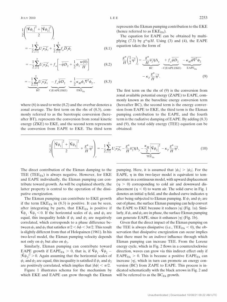
Figure 1 illustrates schema for the mechanism by

which EKE and EAPE can grow through the Ekman

pumping. Here, it is assumed that jc1j . jc2j. For the

EAPE, h in this two-layer model is equivalent to tem-

perature in a continuous model, with upward displacement

(h . 0) corresponding to cold air and downward dis-

placement (h , 0) to warm air. The solid curve in Fig. 1

denotes an initial h field, and the dashed curve indicates h

after being subjected to Ekman pumping. If c1 and c2 are

out of phase, the surface Ekman pumping can help convert

the EAPE to EKE because it reduces jhj (Fig. 1a). Simi-

larly, if c1 and c2 are in phase, the surface Ekman pumping

can generate EAPE, since it enhances jhj (Fig. 1b).

Given that the direct impact of the Ekman pumping on

the TEE is always dissipative (i.e., TEEEk , 0), the ob-

servation that dissipative energization can occur implies

that there must be an indirect influence through which

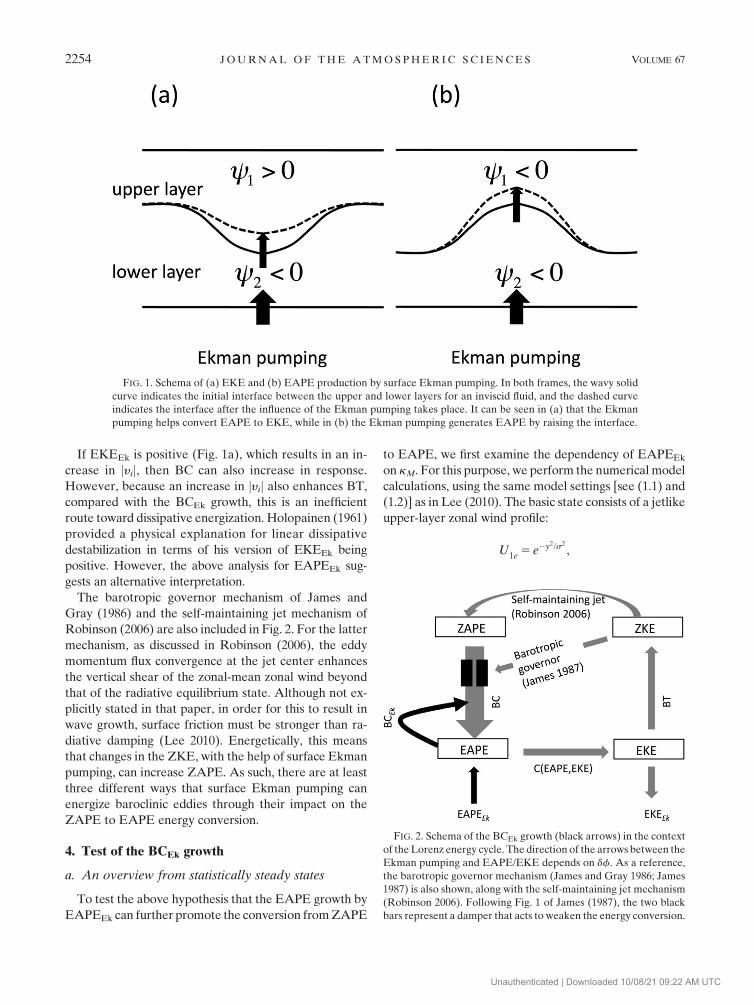
Ekman pumping can increase TEE. From the Lorenz

energy cycle, which in Fig. 2 flows in a counterclockwise

direction, waves can grow via this indirect effect only if

EAPEEk . 0. This is because a positive EAPEEk can

increase jhj, which in turn can promote an energy con-

version (BC) from ZAPE to EAPE. This process is in-

dicated schematically with the black arrows in Fig. 2 and

will be referred to as the BCEk growth.

JULY 2010 L E E 2253


If EKEEk is positive (Fig. 1a), which results in an in-

crease in jyij, then BC can also increase in response.

However, because an increase in jyij also enhances BT,

compared with the BCEk growth, this is an inefficient

route toward dissipative energization. Holopainen (1961)

provided a physical explanation for linear dissipative

destabilization in terms of his version of EKEEk being

positive. However, the above analysis for EAPEEk sug-

gests an alternative interpretation.

The barotropic governor mechanism of James and

Gray (1986) and the self-maintaining jet mechanism of

Robinson (2006) are also included in Fig. 2. For the latter

mechanism, as discussed in Robinson (2006), the eddy

momentum flux convergence at the jet center enhances

the vertical shear of the zonal-mean zonal wind beyond

that of the radiative equilibrium state. Although not ex-

plicitly stated in that paper, in order for this to result in

wave growth, surface friction must be stronger than ra-

diative damping (Lee 2010). Energetically, this means

that changes in the ZKE, with the help of surface Ekman

pumping, can increase ZAPE. As such, there are at least

three different ways that surface Ekman pumping can

energize baroclinic eddies through their impact on the

ZAPE to EAPE energy conversion.

4. Test of the BCEk growth

a. An overview from statistically steady states

To test the above hypothesis that the EAPE growth by

EAPEEk can further promote the conversion from ZAPE

to EAPE, we first examine the dependency of EAPEEk

on kM. For this purpose, we perform the numerical model

calculations, using the same model settings [see (1.1) and

(1.2)] as in Lee (2010). The basic state consists of a jetlike

upper-layer zonal wind profile:

U1e

5 e�y2/s2

,

FIG. 1. Schema of (a) EKE and (b) EAPE production by surface Ekman pumping. In both frames, the wavy solid

curve indicates the initial interface between the upper and lower layers for an inviscid fluid, and the dashed curve

indicates the interface after the influence of the Ekman pumping takes place. It can be seen in (a) that the Ekman

pumping helps convert EAPE to EKE, while in (b) the Ekman pumping generates EAPE by raising the interface.

FIG. 2. Schema of the BCEk growth (black arrows) in the context

of the Lorenz energy cycle. The direction of the arrows between the

Ekman pumping and EAPE/EKE depends on df. As a reference,

the barotropic governor mechanism (James and Gray 1986; James

1987) is also shown, along with the self-maintaining jet mechanism

(Robinson 2006). Following Fig. 1 of James (1987), the two black

bars represent a damper that acts to weaken the energy conversion.



where y 5 0 is at the middle of the channel and s2 5 10.

The equilibrium lower-level wind U2e is set to zero ev-

erywhere. For all simulations to be presented here, kT

and n are fixed at 3021 and 5 3 1024, respectively. The

width of the channel is 30, and there are 200 grid points

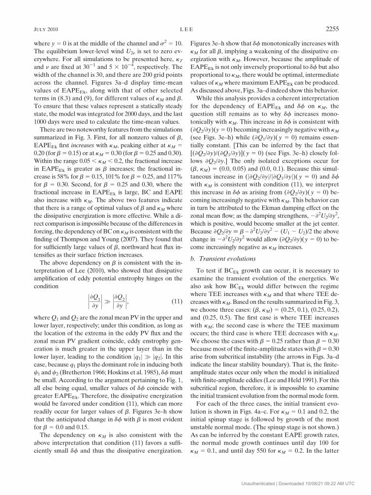
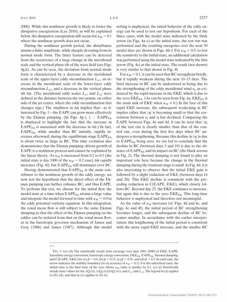
across the channel. Figures 3a–d display time-mean

values of EAPEEk, along with that of other selected

terms in (8.3) and (9), for different values of kM and b.

To ensure that these values represent a statically steady

state, the model was integrated for 2000 days, and the last

1000 days were used to calculate the time-mean values.

There are two noteworthy features from the simulations

summarized in Fig. 3. First, for all nonzero values of b,

EAPEEk first increases with kM, peaking either at kM 5

0.20 (for b 5 0.15) or at kM 5 0.30 (for b 5 0.25 and 0.30).

Within the range 0.05 , kM , 0.2, the fractional increase

in EAPEEk is greater as b increases; the fractional in-

crease is 58% for b 5 0.15, 101% for b 5 0.25, and 117%

for b 5 0.30. Second, for b 5 0.25 and 0.30, where the

fractional increase in EAPEEk is large, BC and EAPE

also increase with kM. The above two features indicate

that there is a range of optimal values of b and kM where

the dissipative energization is more effective. While a di-

rect comparison is impossible because of the differences in

forcing, the dependency of BC on kM is consistent with the

finding of Thompson and Young (2007). They found that

for sufficiently large values of b, northward heat flux in-

tensifies as their surface friction increases.

The above dependency on b is consistent with the in-

terpretation of Lee (2010), who showed that dissipative

amplification of eddy potential enstrophy hinges on the

condition

›Q1

›y

��

��

›Q2

›y

��

��, (11)

where Q1 and Q2 are the zonal mean PV in the upper and

lower layer, respectively; under this condition, as long as

the location of the extrema in the eddy PV flux and the

zonal mean PV gradient coincide, eddy enstrophy gen-

eration is much greater in the upper layer than in the

lower layer, leading to the condition jq1j � jq2j. In this

case, because q1 plays the dominant role in inducing both

c1 and c2 (Bretherton 1966; Hoskins et al. 1985), df must

be small. According to the argument pertaining to Fig. 1,

all else being equal, smaller values of df coincide with

greater EAPEEk. Therefore, the dissipative energization

would be favored under condition (11), which can more

readily occur for larger values of b. Figures 3e–h show

that the anticipated change in df with b is most evident

for b 5 0.0 and 0.15.

The dependency on kM is also consistent with the

above interpretation that condition (11) favors a suffi-

ciently small df and thus the dissipative energization.

Figures 3e–h show that df monotonically increases with

kM for all b, implying a weakening of the dissipative en-

ergization with kM. However, because the amplitude of

EAPEEk is not only inversely proportional to df but also

proportional to kM, there would be optimal, intermediate

values of kM where maximum EAPEEk can be produced.

As discussed above, Figs. 3a–d indeed show this behavior.

While this analysis provides a coherent interpretation

for the dependency of EAPEEk and df on kM, the

question still remains as to why df increases mono-

tonically with kM. This increase in df is consistent with

(›Q2/›y)(y 5 0) becoming increasingly negative with kM

(see Figs. 3e–h) while (›Q1/›y)( y 5 0) remains essen-

tially constant. [This can be inferred by the fact that

[(›Q2/›y)/(›Q1/›y)]( y 5 0) (see Figs. 3e–h) closely fol-

lows ›Q2/›y.] The only isolated exceptions occur for

(b, kM) 5 (0.0, 0.05) and (0.0, 0.1). Because this simul-

taneous increase in (j›Q2/›yj/j›Q1/›yj)( y 5 0) and df

with kM is consistent with condition (11), we interpret

this increase in df as arising from (›Q2/›y)( y 5 0) be-

coming increasingly negative with kM. This behavior can

in turn be attributed to the Ekman damping effect on the

zonal mean flow; as the damping strengthens, 2›2U2/›y2,

which is positive, would become smaller at the jet center.

Because ›Q2/›y [ b – ›2U2/›y2 2 (U1 2 U2)/2 the above

change in 2›2U2/›y2 would allow (›Q2/›y)(y 5 0) to be-

come increasingly negative as kM increases.

b. Transient evolutions

To test if BCEk growth can occur, it is necessary to

examine the transient evolution of the energetics. We

also ask how BCEk would differ between the regime

where TEE increases with kM and that where TEE de-

creases with kM. Based on the results summarized in Fig. 3,

we choose three cases: (b, kM) 5 (0.25, 0.1), (0.25, 0.2),

and (0.25, 0.5). The first case is where TEE increases

with kM; the second case is where the TEE maximum

occurs; the third case is where TEE decreases with kM.

We choose the cases with b 5 0.25 rather than b 5 0.30

because most of the finite-amplitude states with b 5 0.30

arise from subcritical instability (the arrows in Figs. 3a–d

indicate the linear stability boundary). That is, the finite-

amplitude states occur only when the model is initialized

with finite-amplitude eddies (Lee and Held 1991). For this

subcritical region, therefore, it is impossible to examine

the initial transient evolution from the normal mode form.

For each of the three cases, the initial transient evo-

lution is shown in Figs. 4a–c. For kM 5 0.1 and 0.2, the

initial spinup stage is followed by growth of the most

unstable normal mode. (The spinup stage is not shown.)

As can be inferred by the constant EAPE growth rates,

the normal mode growth continues until day 100 for

kM 5 0.1, and until day 550 for kM 5 0.2. In the latter

JULY 2010 L E E 2255


case, the linear growth stage is followed by a brief period

(between days 550 and 750) of higher growth rates. Lee and

Held (1991) interpreted this behavior in terms of a non-

linear growth (g . 0) in the weakly nonlinear amplitude

equation ›A/›t 5 aA 1 gjAj2A (Pedlosky 1970), where A

is the wave amplitude. The finding in Lee (2010) suggests

that this nonlinear growth may be due to the eddy-driven

baroclinicity (‘‘self-maintaining jet’’ mechanism; Robinson



2006). While this nonlinear growth is likely to foster the

dissipative energization (Lee 2010), as will be explained

below, the dissipative energization still occurs for kM 5 0.1

where the nonlinear growth does not occur.

During the nonlinear growth period, the disturbance

attains a finite amplitude, while sharply deviating from its

normal mode form. The latter feature can be detected

from the occurrence of a large change in the meridional

scale and the vertical phase tilt of the wave field (see Figs.

4g,h). As can be seen, the deviation from normal mode

form is characterized by a decrease in the meridional

scale of the upper-layer eddy streamfunction Ly1, an in-

crease in the meridional scale of the lower-layer eddy

streamfunction Ly2, and a decrease in the vertical phase

tilt df. (The meridional eddy scales Ly1 and Ly2 were

defined as the distance between the two points, on either

side of the jet center, where the eddy streamfunction first

changes sign.) The smallness in df implies that—as il-

lustrated by Fig. 1—the EAPE can grow more effectively

by the Ekman pumping. (In Figs. 4g–i, 1 2 EAPEEk

is displayed to highlight the fact that the increase in

EAPEEk is associated with the decrease in df.) In fact,

EAPEEk, while smaller than BC initially, rapidly in-

creases afterward; during the equilibrium stage EAPEEk

is about twice as large as BC. This time evolution also

demonstrates that the Ekman pumping–driven growth of

EAPE is a nonlinear process and cannot be explained by

the linear theory. As kM is increased from 0.2 to 0.5 (the

initial state is day 1000 of the kM 5 0.2 case), df rapidly

increases (Fig. 4i), but EAPEEk still dominates over BC.

Having demonstrated that EAPEEk is the main con-

tributor to the nonlinear growth of the eddy energy, we

now test the hypothesis that the direct effect of the Ek-

man pumping can further enhance BC, and thus EAPE.

To perform this test, we choose for the initial flow the

model state at a time when EAPEEk attains a large value

and integrate the model forward in time with kM 5 0.0 in

the eddy potential vorticity equation. In this integration,

the zonal mean flow is still subject to the same Ekman

damping so that the effect of the Ekman pumping on the

eddies can be isolated from that on the zonal mean flow,

as in the barotropic governor mechanism of James and

Gray (1986) and James (1987). Although this model

setting is unphysical, the initial behavior of the eddy en-

ergy can be used to test our hypothesis. For each of the

three cases, with the model state indicated by the thick

arrow (in Figs. 4a–c) as the initial state, the test run was

performed and the resulting energetics over the next 50

model days are shown in Figs. 4d–f. For kM 5 0.5, to test

the sensitivity to the initial state, an additional calculation

was performed using the model state indicated by the thin

arrow (Fig. 4c) as the initial state. The result (not shown)

is very similar to that shown in Fig. 4f.

For kM 5 0.1, it can be seen that BC strengthens briefly,

but it rapidly weakens during the next 10–15 days. The

brief increase in BC can be understood as being due to

the strengthening of the eddy meridional wind yj, as evi-

denced by the rapid increase in the EKE, which is due to

the zero EKEEk. (As can be seen from Fig. 4a, EKEEk is

the main sink of EKE when kM 6¼ 0.) In the face of this

rapid EKE increase, the subsequent weakening in BC

implies either that jhj is becoming small or that the cor-

relation between yj and h has declined. Comparing the

EAPE between Figs. 4a and 4d, it can be seen that jhjof the test run is clearly smaller than that of the con-

trol run, even during the first five days when BC un-

dergoes a strengthening. Because this decline in jhj is due

to EAPEEk being zero, we are led to conclude that the

decline in BC (between days 3 and 18) is due to the ab-

sence of EAPEEk and its impact on BC (the black arrows

in Fig. 2). The thermal damping is not found to play an

important role here because the change in the thermal

damping during the transient stage is small. In Fig. 4d, it is

also interesting to observe that the initial EKE gain is

followed by a slight reduction of EKE (between days 14

and 20). This EKE decline is consistent with the pre-

ceding reduction in C(EAPE, EKE), which closely fol-

lows BC. Beyond day 25, the EKE continues to increase,

but again this is due to the zero EKEEk. This long-time

behavior is unphysical and therefore not meaningful.

As the value of kM increases (cf. Figs. 4d and 4e, and

Figs. 4e and 4f), the initial period of BC strengthening

becomes longer, and the subsequent decline of BC be-

comes smaller. In accordance with the earlier interpre-

tation, this lengthening of the initial period is consistent

with the more rapid EKE increase, and the smaller BC

FIG. 3. (a)–(d) The statistically steady state (average over days 1001–2000) of EKE, EAPE,

baroclinic energy conversion, barotropic energy conversion, EKEEk, EAPEEk, thermal damping,

and C(EAPE, EKE) for (a) b 5 0.0, (b) b 5 0.15, (c) b 5 0.25, and (d) b 5 0.3. In each case, the

arrow indicates the stability boundary (to an accuracy of kM 5 0.1). For the subcritical cases, the

initial state is the final state of the case whose kM value is smaller by 0.1. (e)–(i) Statistically

steady-state values for df, ›Q2/›y, (›Q2/›y)/(›Q1/›y), and Ly1 and Ly2. The legend in (a) applies

to (b)–(d), and that in (e) applies to (f)–(i).

JULY 2010 L E E 2257


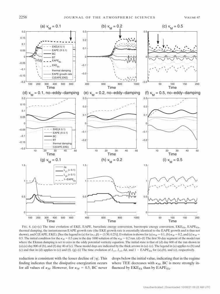
reduction is consistent with the lesser decline of jhj. This

finding indicates that the dissipative energization occurs

for all values of kM. However, for kM 5 0.5, BC never

drops below the initial value, indicating that in the regime

where TEE decreases with kM, BC is more strongly in-

fluenced by EKEEk than by EAPEEk.

FIG. 4. (a)–(c) The time evolution of EKE, EAPE, baroclinic energy conversion, barotropic energy conversion, EKEEk, EAPEEk,

thermal damping, the instantaneous EAPE growth rate (the EKE growth rate is essentially identical to the EAPE growth and is thus not

shown), and C(EAPE, EKE). [See the legend in (a) for (kT, b) 5 (1/30, 0.25)]. Evolution is shown for (a) kM 5 0.1, (b) kM 5 0.2, and (c) kM 5

0.5. The initial condition for the kM 5 0.5 case is the day 1000 solution of the kM 5 0.2 run. (d)–(f) The first 50-day segment of the model run

where the Ekman damping is set to zero in the eddy potential vorticity equation. The initial state is that of (d) day 600 of the run shown in

(a),(e) day 800 of (b), and (f) day 40 of (c). These model days are indicated by the thick arrows in (a)–(c). The legend in (a) applies to (b) and

(c) and that in (d) applies to (e) and (f). (g)–(i) The time evolution of Ly1, Ly2, df, and 1 2 EAPEEk for (a),(b), and (c), respectively.



5. Conclusions

In this study, we investigated how nonlinear dissipative

energization of baroclinic waves occurs in a two-layer

model where Ekman damping is applied only to the lower

layer. Because the total eddy energy of this system is al-

ways damped by the Ekman pumping, the nonlinear

growth must arise from an enhanced interaction via the

Ekman pumping between the eddies and the zonal mean

flow. It is found that this growth involves the following

process:

1) If the phase difference between the upper- and lower-

layer eddies is less than one quarter wavelength, then

the lower-layer Ekman pumping can act to produce

EAPE (EAPEEk . 0) while damping the EKE.

2) This EAPE production in turn increases the baro-

clinic energy conversion (BC) from the ZAPE to the

EAPE.

This BCEk growth can amplify the baroclinic waves if the

net energy production of steps 1 and 2 exceeds the dissi-

pative effect of the Ekman pumping on the EKE. In

principle, this mechanism can be tested by comparing

baroclinic waves in two parallel calculations, one with and

the other without Ekman pumping. However, such a test

cannot be performed with a statistically steady state be-

cause such a state does not exist if kM 5 0. However,

transient wave evolutions found in the no-eddy-damping

experiments support the above interpretation: the ener-

gization occurs because Ekman pumping helps tap ZAPE,

and this additional tapping of ZAPE overcompensates for

the Ekman damping of EKE. Because the direct effect of

the Ekman pumping on the total eddy energy is always

dissipative, although not examined in this study, it is rea-

sonable to expect that the same BCEk growth process may

also operate in the linear dissipative destabilization found

by Holopainen (1961), Pedlosky (1983), and Weng and

Barcilon (1991).

The relationships between the eddy scale and df, and

between df and EAPEEk, as discussed earlier, imply that

eddy scale and EAPEEk may also be related to each other.

For the three nonzero b cases considered in this study, as

can be seen by comparing the eddy scales shown in Figs.

3f–h with the corresponding EAPEEk values in Figs. 3b–d,

there is a hint that Ly1 tends to be relatively small when

EAPEEk is relatively large. Lee (2010) showed that the

reduction in df (Figs. 4g,h) coincides with jetward move-

ments of upper-layer critical lines and confinement of the

upper-layer eddy PV flux toward the jet center. The in-

terpretation of this behavior was that this confinement of

the PV flux, in the region where ›Q1/›y is also large (›Q1/

›y is maximum at the jet center), favors the occurrence of

the inequality in (11). This interpretation can explain the

apparent inverse relationship between Ly1 and EAPEEk.

One implication of this conclusion is that in the presence

of surface Ekman pumping, there is a selective generation

of small scales in the upper layer. It would be interesting to

investigate whether this process can help explain the

finding of Riviere et al. (2004) that bottom friction results

in significant horizontal scale selection.

Acknowledgments. This study was supported by the

National Science Foundation under Grant ATM-0647776.

The author acknowledges valuable comments from Steven

Feldstein and two anonymous reviewers.

REFERENCES

Bretherton, F. P., 1966: Baroclinic instability and the short wave-

length cut-off in terms of potential vorticity. Quart. J. Roy.

Meteor. Soc., 92, 335–345.

Charney, J. G., and A. Eliassen, 1949: A numerical method for pre-

dicting the perturbations of the middle latitude westerlies. Tellus,

1, 38–54.

Eady, E. T., 1949: Long waves and cyclone waves. Tellus, 1, 33–52.

Held, I. M., and V. D. Larichev, 1996: Scaling theory for horizon-

tally homogeneous, baroclinically unstable flow on a beta plane.

J. Atmos. Sci., 53, 945–952.

Holopainen, E. O., 1961: On the effect of friction in baroclinic

waves. Tellus, 13, 363–367.

Hoskins, B. J., M. E. McIntyre, and A. W. Robertson, 1985: On the

use and significance of isentropic potential vorticity maps.

Quart. J. Roy. Meteor. Soc., 111, 877–946.

Hua, B. L., and D. B. Haidvogel, 1986: Numerical simulations

of the vertical structure of quasi-geostrophic turbulence.

J. Atmos. Sci., 43, 2923–2936.

James, I. N., 1987: Suppression of baroclinic instability in hori-

zontally sheared flows. J. Atmos. Sci., 44, 3710–3720.

——, and L. J. Gray, 1986: Concerning the effect of surface drag on

the circulation of a baroclinic planetary atmosphere. Quart.

J. Roy. Meteor. Soc., 112, 1231–1250.

Lapeyre, G., and I. M. Held, 2003: Diffusivity, kinetic energy dis-

sipation, and closure theories for the poleward eddy heat flux.

J. Atmos. Sci., 60, 2907–2916.

Lee, S., 2010: Finite-amplitude equilibration of baroclinic waves on

a jet. J. Atmos. Sci., 67, 434–451.

——, and I. M. Held, 1991: Subcritical instability and hysteresis in

a two-layer model. J. Atmos. Sci., 48, 1071–1077.

Lorenz, E. N., 1955: Available potential energy and the mainte-

nance of the general circulation. Tellus, 7, 157–167.

Pedlosky, J., 1970: Finite-amplitude baroclinic waves. J. Atmos.

Sci., 27, 15–30.

——, 1983: The growth and decay of finite-amplitude baroclinic

waves. J. Atmos. Sci., 40, 1863–1876.

Riviere, P., A. M. Treguier, and P. Klein, 2004: Effects of bottom

friction on nonlinear equilibration of an oceanic baroclinic jet.

J. Phys. Oceanogr., 34, 416–432.

Robinson, W. A., 2006: On the self-maintenance of midlatitude

jets. J. Atmos. Sci., 63, 2109–2122.

Thompson, A. F., and W. R. Young, 2007: Two-layer baroclinic

eddy heat fluxes: Zonal flows and energy balance. J. Atmos.

Sci., 64, 3214–3231.

Weng, H.-Y., and A. Barcilon, 1991: Asymmetric Ekman

dissipation, sloping boundaries and linear baroclinic in-

stability. Geophys. Astrophys. Fluid Dyn., 59, 1–24.

JULY 2010 L E E 2259


Documents

Dissipative Energization of Baroclinic Waves by Surface