Embed Size (px)
Citation preview

Dissipation and dispersion controlof a quadratic-reconstruction advection scheme
Alexandre CARABIAS Alain DERVIEUX
INRIA Sophia-AntipolisProject TROPICS
European Workshop on High Order Nonlinear Numerical Methods forEvolutionary PDEs: Theory and Applications, Trento, Italy, april 11-15, 2011
1 Carabias, Dervieux Dissipation and dispersion control of a quadratic-reconstruction advection scheme

Motivations (1)
Context of the present study
In Fluid Mechanics, most industrial computations are performed with second-orderaccurate schemes but do not enjoy second order numerical convergence (as forexample measured by the Convergence Grid Index).
Reasons are singularities or more generally too many details (of various scales) tocapture.
Consequences are waste (of theoretical accuracy) and less chances to evaluate error.
2 Carabias, Dervieux Dissipation and dispersion control of a quadratic-reconstruction advection scheme
Motivations (2)
Some conditions for an fiable numerical convergence, possibly close to thetheoretical one:- anisotropic mesh adaption,- governed by an error analysis (from a well-specified goal)
High-Accuracy Edge-Based scheme (Cf. T. Kozubskaya’s talk) with TVD limiter.[Loseille-Alauzet-Dervieux,JCP-2010]
0.5M 1M 2M 3M 4M 6M 8M 10M 1
2
3
4
5
6789
10
15
20low drag jet
MACH L2 CONVORDER 2
3 Carabias, Dervieux Dissipation and dispersion control of a quadratic-reconstruction advection scheme

Motivations (3): advection, first example
Level set adaptive tracking in an unstructured mesh
- High-Accuracy Edge-Based scheme (HAEB) with no limiter.
- Second order numerical convergence.
[Guegan-Allain-Dervieux-Alauzet,IJNME-2010]
4 Carabias, Dervieux Dissipation and dispersion control of a quadratic-reconstruction advection scheme
Motivations (4): advection, second example
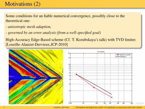
Acoustics wave adaptive capturing in an unstructured mesh
- HAEB with no limiter.- Second order numerical convergence.
[Belme et al. to appear]
5 Carabias, Dervieux Dissipation and dispersion control of a quadratic-reconstruction advection scheme
Towards a better advection scheme
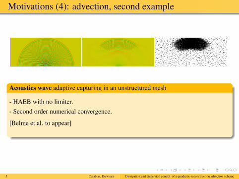
The three previous examples were performed with HAEB scheme presented by T.Kozubskaya and enjoying:- low dissipation (fifth-order accurate on cartesian meshes)- only second-order accurate on unstructured meshes,
Requirements for a better scheme
Coarse mesh accuracy, low dissipation, small computing effort for a given mesh:- Central-ENO (cf. C. Groth) reconstruction,- Vertex centered approximation,
6 Carabias, Dervieux Dissipation and dispersion control of a quadratic-reconstruction advection scheme

Plan of the talk
1. Baseline 2D quadratic scheme.
2. Analysis and improvement of a 1D context.
3. Extension to 2D.
4. Preliminary numerical experiments.
7 Carabias, Dervieux Dissipation and dispersion control of a quadratic-reconstruction advection scheme

1. Baseline scheme (1)
Vertex, dual cell, 2-exact Central-ENO quadratic reconstruction
Given ui on on each cell i of centroid Gi, find the ci,α , |α| ≤ k such that
Pi,i = ui ∑j∈N(i)
(Pi,j−uj)2 = Min
withPi(x) = ui + ∑
|α|≤kci,α [(X−Gi)α − (X−Gi)α ]
and where Pi,j stands for the mean of Pi(x) on cell j.
8 Carabias, Dervieux Dissipation and dispersion control of a quadratic-reconstruction advection scheme

1. Baseline scheme (2)
2-exact flux integration
The integral on a cell interface Cij = Ci∩Cj is split into the integrals on the twosegments of Cij.On each segment C(1)
ij and C(2)ij a numerical integration with two Gauss points (two
Riemann solvers) is applied.
9 Carabias, Dervieux Dissipation and dispersion control of a quadratic-reconstruction advection scheme

1. Baseline scheme (3)
Computational cost, fixed mesh
Computational cost is minimised by computing and storing reconstruction topology,coefficients and inverse matrix.This needs be done each time mesh is changed.In these conditions, the quadratic reconstruction scheme at each time step needs foreach flux evaluation between two cells:
4 Riemann solutions,where 1 is needed with the HAEB. We have check that the overall CPU ratio ismore than 4.
Computational cost, changing mesh
In the case of a moving mesh the ratio between MUSCL and quadratic is more than6.
These are 2D measures and should much amplify for 3D.
10 Carabias, Dervieux Dissipation and dispersion control of a quadratic-reconstruction advection scheme

1. Baseline scheme (4)
A test case: C.Tam’s test for linear acoustics[Ouvrard-Kozubskaya-Abalakin-Koobus-Dervieux, INRIA Rep. 2009]- 12 ∆x per bandwidth, three types of mesh.- black: HAEB scheme,- Blue: the present CENO2 scheme.
Mesh1 Mesh1 Mesh2 Mesh2 Mesh3 Mesh3L1 L2 L1 L2 L1 L2
1.3045D-3 2.8561D-3 1.2786D-3 2.6318D-3 3.1097D-3 5.9216D-31.5189D-4 3.4010D-4 3.7384D-4 2.6318D-3 6.7626D-4 1.4598D-3
11 Carabias, Dervieux Dissipation and dispersion control of a quadratic-reconstruction advection scheme
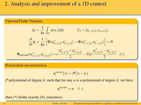
2. Analysis and improvement of a 1D context
Upwind Finite Volumes
ui =1
∆x
∫Ci
u(x, t)dx Ci = [xi−1/2,xi+1/2].
∂
∂ tui +
1∆x
[Φ(u+
i+1/2,u−i+1/2)−Φ(u+
i−1/2,u−i−1/2)
]= 0
Φupwind(u+i+1/2,u
−i+1/2) = c
u+i+1/2 +u−i+1/2
2−δ |c|
u+i+1/2−u−i+1/2
2(∗)
Polynomial reconstruction
ureconsi (x) = Pu
i (x− xi)
P polynomial of degree k, such that for any u is a polynomial of degree k, we have
ureconsi = u ∀ i,
then (*) holds exactly (Pk exactness).12 Carabias, Dervieux Dissipation and dispersion control of a quadratic-reconstruction advection scheme

Analysis and improvement of a 1D context (2)
For example, with a quadratic reconstruction and uniform mesh:
ureconsi (x) = ci +bi(x− xi)+ai(x− xi)2
ai =ui+1−2ui + ui−1
2∆x2
bi =ui+1− ui−1
2∆x
ci =−ui+1 +2ui− ui−1
24+ ui
13 Carabias, Dervieux Dissipation and dispersion control of a quadratic-reconstruction advection scheme

Analysis and improvement of a 1D context (3)
Spatial truncation analysis
ui = ui +u(2)i
∆x2
24+u(4)
i∆x4
1920+O
(∆x6).
∫Ci
∂u∂x
dx− 1∆x
[Φ(u+
i+1/2,u−i+1/2)−Φ(u+
i−1/2,u−i−1/2)
]=
−δ |c|12
(∆x)3u(4) +|c|30
(∆x)4u(5) +O(∆x6).
- Diffusion is the largest term of truncation error, with a large influence for coarsemeshes.- Dispersion vs diffusion balance contributes to the “Essentially Non Oscillating”effect which masters the possible oscillations provoked by singularities.- This balance makes diffusion unnecessarily large for smooth solutions.
14 Carabias, Dervieux Dissipation and dispersion control of a quadratic-reconstruction advection scheme
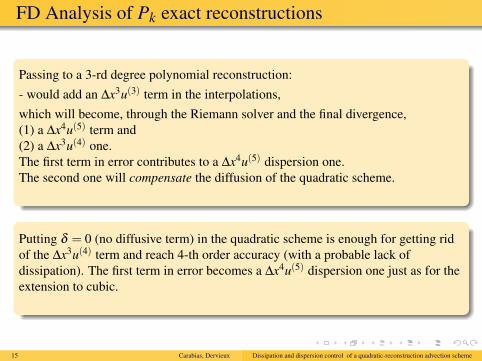
FD Analysis of Pk exact reconstructions
Passing to a 3-rd degree polynomial reconstruction:- would add an ∆x3u(3) term in the interpolations,which will become, through the Riemann solver and the final divergence,(1) a ∆x4u(5) term and(2) a ∆x3u(4) one.The first term in error contributes to a ∆x4u(5) dispersion one.The second one will compensate the diffusion of the quadratic scheme.
Putting δ = 0 (no diffusive term) in the quadratic scheme is enough for getting ridof the ∆x3u(4) term and reach 4-th order accuracy (with a probable lack ofdissipation). The first term in error becomes a ∆x4u(5) dispersion one just as for theextension to cubic.
15 Carabias, Dervieux Dissipation and dispersion control of a quadratic-reconstruction advection scheme
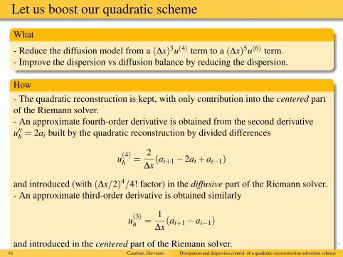
Let us boost our quadratic scheme
What
- Reduce the diffusion model from a (∆x)3u(4) term to a (∆x)5u(6) term.- Improve the dispersion vs diffusion balance by reducing the dispersion.
How- The quadratic reconstruction is kept, with only contribution into the centered partof the Riemann solver.- An approximate fourth-order derivative is obtained from the second derivativeu′′h = 2ai built by the quadratic reconstruction by divided differences
u(4)h =
2∆x
(ai+1−2ai +ai−1)
and introduced (with (∆x/2)4/4! factor) in the diffusive part of the Riemann solver.- An approximate third-order derivative is obtained similarly
u(3)h =
1∆x
(ai+1−ai−1)
and introduced in the centered part of the Riemann solver.16 Carabias, Dervieux Dissipation and dispersion control of a quadratic-reconstruction advection scheme

Introducing 5-th order 6-th derivative diffusion
Reconstruction model:
ureconstr(x+ xi) = uh +u′hx+12
u′′hx2 +13!
u(3)h x3 +
14!
u(4)h x4
uh +u′hx+ 12 u′′hx2 is put in the centered part of Riemann solver,
13! u(3)
h x3 is put in the centered part of Riemann solver,
14! u(4)
h x4 is put in the diffusive part of Riemann solver.
A fifth-order linearised Runge-Kutta explicit time advancing is applied.
Properties of the 1D prototype
The above scheme is fifth-order accurate for uniform meshes.
17 Carabias, Dervieux Dissipation and dispersion control of a quadratic-reconstruction advection scheme
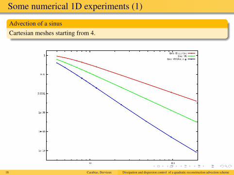
Some numerical 1D experiments (1)
Advection of a sinusCartesian meshes starting from 4.
18 Carabias, Dervieux Dissipation and dispersion control of a quadratic-reconstruction advection scheme

Some numerical 1D experiments (2)
Numerical convergence analysis
Mean values at cell centers: approximate (green) and exact (red)solutions for atravel of 100 wavelengths (CFL=.9) and 12 nodes per wavelength.
– Baseline scheme – Central+V6-diffusion – Central+V6+antidispersion
19 Carabias, Dervieux Dissipation and dispersion control of a quadratic-reconstruction advection scheme
3. Extension to 2D
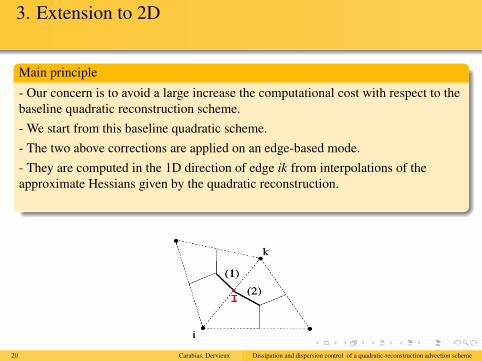
Main principle
- Our concern is to avoid a large increase the computational cost with respect to thebaseline quadratic reconstruction scheme.- We start from this baseline quadratic scheme.- The two above corrections are applied on an edge-based mode.- They are computed in the 1D direction of edge ik from interpolations of theapproximate Hessians given by the quadratic reconstruction.
20 Carabias, Dervieux Dissipation and dispersion control of a quadratic-reconstruction advection scheme
Extension to 2D (3)
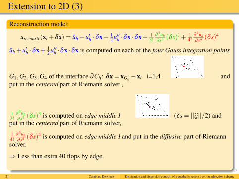
Reconstruction model:
ureconstr(xi +δx) = uh +u′h ·δx+ 12 u′′h ·δx ·δx+ 1
3!∂ 3uh∂ s3 (δ s)3 + 1
4!∂ 4uh∂ s4 (δ s)4
uh +u′h ·δx+ 12 u′′h ·δx ·δx is computed on each of the four Gauss integration points
G1,G2,G3,G4 of the interface ∂Cij: δx = xGk −xi i=1,4 andput in the centered part of Riemann solver ,
13!
∂ 3uh∂ s3 (δ s)3 is computed on edge middle I (δ s = ||ij||/2) and
put in the centered part of Riemann solver,
14!
∂ 4uh∂ s4 (δ s)4 is computed on edge middle I and put in the diffusive part of Riemann
solver.
⇒ Less than extra 40 flops by edge.
21 Carabias, Dervieux Dissipation and dispersion control of a quadratic-reconstruction advection scheme

4. Some preliminary numerical experiments
4.1.-Advection of a Gaussian
4.2.-Advection of the isovalue of a two-Gaussian camel hump.
22 Carabias, Dervieux Dissipation and dispersion control of a quadratic-reconstruction advection scheme

4. Numerical experiments (1)
Numerical experiments
Convection of a Gaussian concentration, structured meshes.
23 Carabias, Dervieux Dissipation and dispersion control of a quadratic-reconstruction advection scheme
4. Numerical experiments (1)
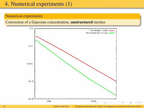
Numerical experiments
Convection of a Gaussian concentration, unstructured meshes
24 Carabias, Dervieux Dissipation and dispersion control of a quadratic-reconstruction advection scheme
4. Numerical experiments (3)
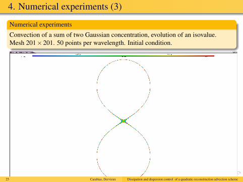
Numerical experiments
Convection of a sum of two Gaussian concentration, evolution of an isovalue.Mesh 201×201. 50 points per wavelength. Initial condition.
25 Carabias, Dervieux Dissipation and dispersion control of a quadratic-reconstruction advection scheme
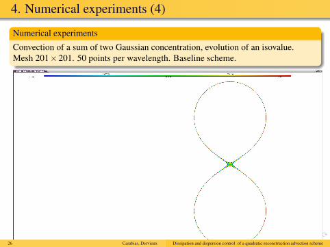
4. Numerical experiments (4)
Numerical experiments
Convection of a sum of two Gaussian concentration, evolution of an isovalue.Mesh 201×201. 50 points per wavelength. Baseline scheme.
26 Carabias, Dervieux Dissipation and dispersion control of a quadratic-reconstruction advection scheme
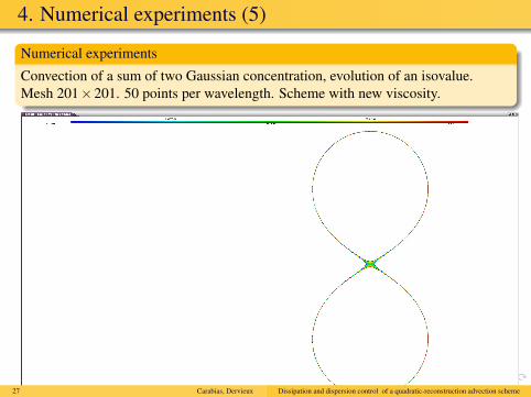
4. Numerical experiments (5)
Numerical experiments
Convection of a sum of two Gaussian concentration, evolution of an isovalue.Mesh 201×201. 50 points per wavelength. Scheme with new viscosity.
27 Carabias, Dervieux Dissipation and dispersion control of a quadratic-reconstruction advection scheme
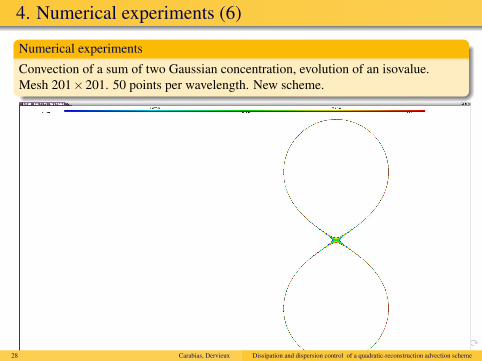
4. Numerical experiments (6)
Numerical experiments
Convection of a sum of two Gaussian concentration, evolution of an isovalue.Mesh 201×201. 50 points per wavelength. New scheme.
28 Carabias, Dervieux Dissipation and dispersion control of a quadratic-reconstruction advection scheme

4. Numerical experiments (7)
Numerical experiments
Convection of a sum of two Gaussian concentration, evolution of an isovalue.Mesh 21×21. 5 points per wavelength. Initial condition.
29 Carabias, Dervieux Dissipation and dispersion control of a quadratic-reconstruction advection scheme

4. Numerical experiments (8)
Numerical experiments
Convection of a sum of two Gaussian concentration, evolution of an isovalue.Mesh 201×201. 5 points per wavelength. Baseline scheme.
30 Carabias, Dervieux Dissipation and dispersion control of a quadratic-reconstruction advection scheme

4. Numerical experiments (9)
Numerical experiments
Convection of a sum of two Gaussian concentration, evolution of an isovalue.Mesh 21×21. 5 points per wavelength. Scheme with new viscosity.
31 Carabias, Dervieux Dissipation and dispersion control of a quadratic-reconstruction advection scheme
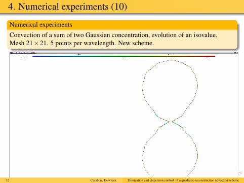
4. Numerical experiments (10)
Numerical experiments
Convection of a sum of two Gaussian concentration, evolution of an isovalue.Mesh 21×21. 5 points per wavelength. New scheme.
32 Carabias, Dervieux Dissipation and dispersion control of a quadratic-reconstruction advection scheme

5. Extension to the Euler’s equations (1)
Euler equations
∂W∂ t
+∇.F(W) = 0,
with W = (ρ,ρu,ρv,ρw,ρE)t is the conservative variable vector and F is theconvection operator F(W) =
(F1(W),F2(W),F3(W)
):
Convection operator
F1(W) =
ρu
ρu2 +pρuvρuw
(ρE +p)u
, F2(W) =
ρvρuv
ρv2 +pρvw
(ρE +p)v
, F3(W) =
ρw
ρuwρvw
ρw2 +p(ρE +p)w
.
33 Carabias, Dervieux Dissipation and dispersion control of a quadratic-reconstruction advection scheme

5. Extension to the Euler’s equations (2)
Finite Volume applied to Euler’s Equation
|Ci|dWi
dt+∫
∂Ci
F(Wi).nidγ−∫
Γh∩∂Ci
F(Wi).nΓhdΓh = 0,
Convective Flux∫∂Ci
F(Wni ).nidγ = ∑
vj∈ϑ(vi)F|Iij .
∫∂Cij
nidγ = ∑vj∈ϑ(vi)
Φ(Wi,Wj,nij),
Γij = Γij(Wi,Wj,nij) = F|Iij .∫
∂Cij
nidγ,
Γij(Wi,Wj,~nij) =F(Wi)+F(Wj)
2.nij +d(Wi,Wj,nij),
34 Carabias, Dervieux Dissipation and dispersion control of a quadratic-reconstruction advection scheme
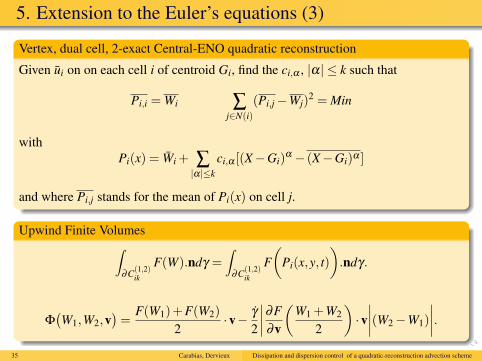
5. Extension to the Euler’s equations (3)
Vertex, dual cell, 2-exact Central-ENO quadratic reconstruction
Given ui on on each cell i of centroid Gi, find the ci,α , |α| ≤ k such that
Pi,i = Wi ∑j∈N(i)
(Pi,j−Wj)2 = Min
withPi(x) = Wi + ∑
|α|≤kci,α [(X−Gi)α − (X−Gi)α ]
and where Pi,j stands for the mean of Pi(x) on cell j.
Upwind Finite Volumes∫∂C(1,2)
ik
F(W).ndγ =∫
∂C(1,2)ik
F(
Pi(x,y, t))
.ndγ.
Φ(W1,W2,v
)=
F(W1)+F(W2)2
·v− γ
2
∣∣∣∣∂F∂v
(W1 +W2
2
)·v∣∣∣∣(W2−W1)
∣∣∣∣.35 Carabias, Dervieux Dissipation and dispersion control of a quadratic-reconstruction advection scheme
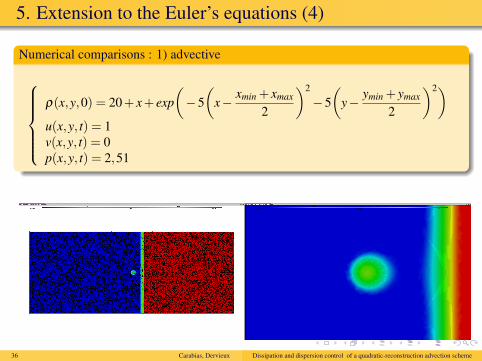
5. Extension to the Euler’s equations (4)
Numerical comparisons : 1) advective
ρ(x,y,0) = 20+ x+ exp
(−5(
x− xmin + xmax
2
)2
−5(
y− ymin + ymax
2
)2)u(x,y, t) = 1v(x,y, t) = 0p(x,y, t) = 2,51
36 Carabias, Dervieux Dissipation and dispersion control of a quadratic-reconstruction advection scheme

5. Extension to the Euler’s equations (4)
Unstructured meshe (40 000 vertex), CFL 0.5
Quadratic scheme (left) and MUSCL V4 (right) for 500 iterations.
37 Carabias, Dervieux Dissipation and dispersion control of a quadratic-reconstruction advection scheme

5. Extension to the Euler’s equations (4)
Numerical comparison : 2) acoustic
Acoustic source define by f = (0,0,0,r) on a 50 000 nodes meshe :
r =−A.exp(−B.ln(2)[x2 + y2]
)C.cos(2Πfr),
38 Carabias, Dervieux Dissipation and dispersion control of a quadratic-reconstruction advection scheme

5. Extension to the Euler’s equations (4)
Muscl V4 (left), quadratic scheme (right), 500 iterations (top), 1000 iteratons(down)
39 Carabias, Dervieux Dissipation and dispersion control of a quadratic-reconstruction advection scheme

End. Concluding remarks
Synthesis
We are studying an advection scheme “for the poor”. It uses a quadraticreconstruction. 4 arithmetic means on Gauss integration points replace the 4Riemann solvers. The rest of flux is made of two cheap HAEB-like terms.
Preliminary accuracy measures show a modest improvement in convergence order.The third-order baseline gives 2.91 to 2.92, the new scheme gives 3.12 to 4.1.
But the improvement is important in constants, for example, for unstructuredmeshes of 2,000 nodes, the error is 3,5 smaller, for 30,000 nodes, 6.5 times smaller.
What next
The new advection scheme will be experimented in combination withHessian-based anisotropic mesh adaptation.
40 Carabias, Dervieux Dissipation and dispersion control of a quadratic-reconstruction advection scheme
Thank you
41 Carabias, Dervieux Dissipation and dispersion control of a quadratic-reconstruction advection scheme

![Project-Team Pulsar Perception Understanding Learning ... · Slawomir Bak [Nice Sophia-Antipolis University, VideoID Grant] Piotr Bilinski [Nice Sophia-Antipolis University, Paca](https://img.pdfslide.us/doc/110x75/5f159bbd220ad72899675965/project-team-pulsar-perception-understanding-learning-slawomir-bak-nice-sophia-antipolis.jpg)