Dissertation

Master in Automotive Engineering

Thermal energy recovery systems for automotive

vehicles: swashplate expander modeling

Vitor Manuel Cerqueira Magro Lopes

Leiria, september of 2015

Dissertation

Master in Automotive Engineering

Thermal energy recovery systems for automotive

vehicles: swashplate expander modeling

Vitor Manuel Cerqueira Magro Lopes

Dissertation of Master developed under the supervision of Professor Hélder Manuel Ferreira Santos, Professor at School of Technology and Management of the Polytecnic Institute of Leiria, and co-supervision of Professor João Francisco Romeiro da Fonseca Pereira.

ii

Leiria, september of 2015

iii

This page was intetionally left blank

iv

Acknowledgements

The first thank goes to my mentor, Professor Hélder Santos, for all the support,

patience, enthusiasm and interest and during all the steps of the work, giving me extra

motivation. His advices and suggestions were very helpful in crucial phases and in some

decisions that needed to be made throughout, and his knowledge was a benefit for the

overall project. I also thank to Professor João Fonseca Pereira for the help and support

throughout the development of the project.

Secondly, I thank a lot to my co mentor Vicente Dolz. I am very grateful for the

opportunity that was given to me by him, by accepting me and mentoring me in the CMT-

Centro de Motores Térmicos. His knowledge in the matter was very helpful and I feel I

learned a lot in the matter of the ORC systems during my internship year. All the

knowledge acquired there was fundamental for this work: theory, logic, software usage and

experimental runs. It was a really great opportunity that was conceded to me.

A big thank goes to my colleague Lucía Royo for all the help, support, for

encouraging me and for being such a good coworker; I also thank to Petar Kleut for

making me feel like home, to Jaime Sánchez, Luís Miguel, Paula, Ana and Teresa.

Another acknowledgement goes to my colleague André Almeida for his advices and

support.

I also thank to my parents Vitor and Aida, and my sister Ana for all their support and

advices and for believing in me no matter what, and for encouraging me to go all the way

and never give up.

v

This page was intetionally left blank

vi

Resumo

No ínicio deste trabalho, foram abordadas algumas questões. O primeiro passo no

desenvolvimento do presente estudo consiste numa extensa revisão literária acerca de

sistemas de recuperação de energia térmica em veículos automóveis. A revisão literária foi

essencial para identificar o ciclo de Rankine como uma solução de elevado potencial para

aplicação em veículos. Foi desenvolvida e apresentada uma metodologia que permite

determinar que tipo de expanser é mais adequado para um dado sistema com ciclo de

Rankine, utilizando o diagrama NsDs. Os parametros que têm influência na seleção do

expansor são: o fluido de trabalho, as condições de entrada e de saída (temperatura,

pressão, tipo de fluido e caudal mássico), a velocidade de rotação e o diâmetro do

expansor. O caudal mássico é calculado de acordo com o intervalo de potência

normalmente obtido através do evaporador instalado em veículos automóveis (de 10 kW a

500 kW). O presente trabalho apresenta uma metodologia que permite a seleção do

expansor para uma dada aplicação. Para isso, foram selecionados três fluidos de trabalho

(R245fa, etanol e água) para demonstrar a metodologia desenvolvida. O modelo

desenvolvido em AMESim foi validado e comparado com resultados obtidos

experimentalmente, que confirmaram a precisão dos mesmos.

Palavras-chave: Sistemas de recuperação de energia térmica, Ciclo de

Rankine, Seleção do Expansor, Fluidos de trabalho, desenvolvimento de um

modelo

vii

This page was intetionally left blank

viii

Abstract

At the beginning of this work, a number of issues had to be addressed. A first step

in the development of the present study consists on the extensive literature review on the

automotive vehicle waste heat recovery systems. The literature review was essential to

identify the Rankine cycle as a high potential solution for vehicle applications. A

methodology was developed and presented in order to determine which type of expander

suits best in a given RC system, using the NsDs turbine chart. The parameters that have

influence on the expander’s selection are: the working fluid inlet and outlet conditions

(such as the temperature, pressure, type of fluid and the mass flow rate), the rotating speed

and the diameter of the expander. The mass flow rate will be calculated according to the

usual power extracted by the evaporator from waste heat recovery systems installed in

automotive vehicles (10 kW to 500 kW). The present work presents a methodology that

allows selecting an expander for a specific application. To this end, three different working

fluids (R245fa, ethanol and water) were selected to demonstrate the developed

methodology. The model developed in AMESim was validated by comparing the results

with the ones obtained through experimental runs, which confirmed its accuracy in the

results obtained.

Keywords: Waste heat recovery, Rankine cycle, Expander selection,

Working fluids, Model development

ix

This page was intetionally left blank

x

List of figures

Figure 2.1 - Overall efficiency of an ICE, Sankey Diagrams (n.d.). ................................................................... 3

Figure 2.2 - a) Schematic representation of a RC system; b) T-s diagram of the ideal RC. ............................... 6

Figure 2.3 – T-H diagram illustrating the Pinch Point Temperature Difference (PPTD). ................................... 7

Figure 2.4 - T-s diagram for different working fluid types: a) isentropic; b) wet; c) dry, Santos et al. (2011). ... 8

Figure 2.5 - T-s diagram of water, ethanol, R245fa and a water-ethanol mixture, adapted from Teng et al.

(2011). ....................................................................................................................................................... 10

Figure 2.6 - Heat exchanger types: left – shell and tube; right – plate and fin, Lopes et al. (2012). ............... 14

Figure 2.7 – Isentropic expansion in PV diagrams: a) under-expansion and b) over-expansion, Kim et al.

(2012). ....................................................................................................................................................... 16

Figure 2.8 - Rankine cycle considering both isentropic expansion and real expansion, Stine & Geyer (2001). 16

Figure 2.9 - Diagram of the various expander types, adapted from Dingel & Ambrosius (2014). .................. 17

Figure 2.10 – Cut-view of a Turbine Expander, Lopes et al. (2012). .............................................................. 21

Figure 2.11 - Vane expanders operation. 1 – intake, 2 and 3 – expansion, 4 – exhaust, Lopes et al. (2012). .. 23

Figure 2.12 - Two main leakage types in a scroll expander, Lopes et al. (2012). ........................................... 25

Figure 2.13 - Scroll expander used in the LT cycle by Kim et al. (2012). ........................................................ 25

Figure 2.14 - Twin Screw Expander, Langson (2008). ................................................................................... 26

Figure 2.15 – Piston expander machine – working principle. ....................................................................... 27

Figure 2.16 – Piston expander machine working principle, Lopes et al. (2012). ............................................ 27

Figure 2.17 – Piston machine diagrams - Top Left: Real PV; Top Right: Ideal PV, Wikipedia (n.d.); Bottom:

Valve Lift.................................................................................................................................................... 28

Figure 2.18 - Swash plate piston expander from Endo et at. (2007). ............................................................ 30

Figure 2.19 - Swash plate piston expander used by Kim et al. (2012). .......................................................... 30

Figure 3.1 - Barber Nichols "how to select turbomachinery for your application", Keneth (1959). ................ 32

Figure 3.2 – Dixon’s turbine chart (adapted from Dixon (1977)). ................................................................. 33

Figure 3.3 – Japikse’s expander machine selection chart (adapted from Sauret & Rowlands (2011)). ........... 33

Figure 3.4 – Diagram that describes the sequence used to calculate de Ns and Ds parameters. ................... 35

Figure 3.5 – Diagram of the process and initial values for calculations. ....................................................... 38

Figure 3.6 – Top: Test condition 1; Center: Test condition 2; Bottom: Test condition 3 (see Table 3.2),

corresponding to the displacement expanders rotary speeds and a diameter of 0,03 m. .............................. 41

Figure 3.7 – Top: Test condition 4; Center: Test condition 5; Bottom: Test condition 6 (see Table 3.2),

corresponding to the turbine expanders rotary speeds and a diameter of 0,03 m. ....................................... 42

Figure 3.8 - Region obtained from the experimental data in the NsDs chart. ............................................... 45

Figure 3.9 – Zoom of the region obtained in the NsDs chart from the experimental data. ............................ 45

xi

Figure 4.1 - Schematic representation of the expander model found in Glavatskaya et al.( 2012). ............... 48

Figure 4.2 – Empirical (black-box) model of the expander modeled for this work......................................... 49

Figure 4.3 – Amesim interface and libraries ................................................................................................ 52

Figure 4.4 – AMESim expander model developed in the present work ......................................................... 54

Figure 4.5 – Scheme used to determine the transformer ratio (l); a) Side view of the Swash Plate; b) Top view

of the swash plate. .................................................................................................................................... 57

Figure 4.6 – Creating batch parameters for simultaneous runs. .................................................................. 62

xii

List of tables

Table 2.1 - Properties of the working fluids that can be used for RC systems. ................................................ 9

Table 2.2 – Values from previous studies found in Lopes et al. (2012). ......................................................... 18

Table 2.3 – Compilation of the data of the system found in Seher et al. (2012). ........................................... 19

Table 2.4 - Technical features of WHR system applied to a HDD engine, Bosch (2012). ................................ 19

Table 2.5 - Resume of the expander types investigated in previous studies. ................................................. 20

Table 3.1 – Resume of the thermodynamic properties................................................................................. 38

Table 3.2 – Rotary speeds used for calculations. ......................................................................................... 39

Table 3.3 – Excel table with the thermodynamic inputs. .............................................................................. 39

Table 3.4 – Excel table with the values for the expander and the resultant specific speed and specific

diameter (test condition 1, see Table 3.2). .................................................................................................. 40

Table 3.5 - ORC operating points for simulation in Galindo et al. (2015). ..................................................... 44

Table 4.1 – Softwares used by authors in previous studies. ......................................................................... 50

Table 4.2 – Components for the inputs ....................................................................................................... 55

Table 4.3 – Components for computing the valve and port opening and closing. ......................................... 56

Table 4.4 – Components used to convert the rotary speed into linear velocity. ............................................ 58

Table 4.5 – Components used to model the piston chamber. ....................................................................... 59

Table 4.6 – Component used to select the working fluid of the model. ........................................................ 60

Table 4.7 – Experimental data used for AMESim model validation. ............................................................. 61

xiii

This page was intetionally left blank

xiv

List of acronyms

Latin Characters

speed of sound (340,29 [m/s])

isentropic spouting velocity [m/s]

specific heat at constant pressure [kJ/kg.K]

cte constant [-]

diameter [m]

g acceleration of gravity [ ]

H height [ft] or [m]

specific enthalpy [kJ/kg]

mass flow rate [kg/s]

rotary speed [rpm]

P pressure [Pa]

thermal power [W]

Reynolds number [-]

specific entropy [kJ/kg.K]

temperature [ºC] or [K]

tip speed [m/s]

volumetric flow rate [ /s]

work [J]

Greek Characters

differential

efficiency [-]

Π pressure ratio [-]

ρ density [ /kg]

kinematic viscosity [ /s]

𝛷 flow coefficient (for Japikse’s chart) [-]

Ψ head coefficient (for Japilse’s chart) [-]

xv

Subscripts

ambient

condenser

evaporator

exhaust

inlet

loss

mechanical

mechanical expander

outlet

pump

isentropic

supply

turbine

thermal

Abbreviations

1D One-dimensional

3D Three-dimensional

BC Bottoming Cycle

BDC Bottom Dead Center

CAD Computer aided design

EES Engineering Equation Solver

EGR Exhaust Gas Recirculation

ETC Electric Turbo-Compounding

FEM Finite Element Method

GWP Global Warming Potential

HD Heavy Duty

HDD Heavy Duty Diesel

HT High-temperature

ICE Internal Combustion Engine

IFP Institut Français du Pétrole (French Institute of Petrol)

xvi

ISO International Organization for Standardization

LCA Life-cycle assessment

LiIon Lithium-ion

LT Low-temperature

MTC Mechanical Turbo-Compounding

NFPA National Fire Protection Association

NIST National Institute of Standards and Technology

NPSS Numerical Propulsion System Simulation

ODP Ozone Depletion Potential

ORC Organic Rankine Cycle

PPTD Pinch Point Temperature Difference

PV Pressure-volume

RC Rankine Cycle

rpm Rotation per minute

SI Système International d'Unités (International System of Units)

TIGERS Turbo-Generator Integrated Gas Energy Recovery System

TDC Top Dead Center

VFR Volume flow ratio

WHR Waste Heat Recovery

xvii

This page was intetionally left blank

xviii

Table of contents

ACKNOWLEDGEMENTS IV

RESUMO VI

ABSTRACT VIII

LIST OF FIGURES X

LIST OF TABLES XII

LIST OF ACRONYMS XIV

TABLE OF CONTENTS XVIII

1. INTRODUCTION 1

1.1. Motivation 1

1.2. Goals and Outline 1

1.3. General Contents 2

2. LITERATURE REVIEW 3

2.1. Introduction 3

2.2. Waste Heat Recovery 3

2.3. The Rankine Cycle System 5

2.4. Working Fluids 7

2.5. WHR System Components 12

2.5.1. Pump 13

2.5.2. Heat Exchanger 13

2.5.3. Condenser 14

2.5.4. Expander 15

2.6. Expander Types 17

2.6.1. Dynamic expanders (turbines) 21

xix

2.6.2. Displacement expanders (volumetric) 23

2.6.2.1. Rotary vane expander 23

2.6.2.2. Scroll expander 24

2.6.2.3. Screw expander 26

2.6.2.4. Piston 27

2.6.2.5. Swash-plate piston expander 29

3. EXPANDER SELECTION 31

3.1. Introduction 31

3.2. Selection parameters 31

3.3. Methodology 34

3.4. Selection of an expander for an automotive RC system 37

3.4.1. Influence of the expander’s diameter 43

3.4.2. Expander selection for the present study 44

3.5. Summary 46

4. THE EXPANDER MODEL 47

4.1. Introduction 47

4.2. Different model types 47

4.3. Softwares available 50

4.4. LMS Imagine AMESim 51

4.5. Developed expander model 54

4.6. Model validation 60

5. CONCLUSIONS 63

5.1. Future works 63

REFERENCES 65

APPENDIX 71

1

1. Introduction

1.1. Motivation

Two thirds of the total fuel energy consumed by Internal Combustion Engine (ICE)

is wasted by the cooling circuit and the exhaust. Therefore, if some part of this energy can

be recovered and converted into useful (mechanical or electric) energy, the overall

efficiency of the automotive could be raised and the fuel consumption could be lowered.

Many studies have been performed, particularly on the Organic Rankine cycle (ORC), for

the recovery of the heat energy wasted by the exhaust gases. One of the key components of

this system is the expansion machine, which has a strong impact on the cycle’s

performance. Many expanders have been theoretically studied and simulated, by the means

of softwares and real runs, but only few studies on the reciprocating piston expander as an

expansion machine have been performed until the present. As a result, the present study

approaches the general ORC system with special attention to the expander machine.

1.2. Goals and Outline

The aim of this work is to study and model a swash plate piston expander in the

engineering software AMESim. The main goal is to develop a modelation that will be

calibrated with experimental data, so that, in the future, expensive experimental tests can

be avoided. To achieve this main goal, the present work addresses the following issues:

- Literature review on the ORC for automotive vehicle applications, its components

and the working fluids;

- Describe with detail the expansion process, review the existing expanders and

explain which type of expander is best for a determined application;

- Study the AMESim interface, libraries and how to model an engineering system,

which data can be input and obtained and how to run and extract the results;

- Model the expander and perform a series of runs with the experimental data in

order to adjust and calibrate the final model.

2

1.3. General Contents

This work is organized in five chapters. The chapter 1 introduces the subject of the

present work, explaining the reasons of the study and what steps will be followed in order

to achieve the goals.

Chapter 2 contains a detailed literature review about waste heat recovery technics

developed until today, why the ORC is preferred in automotive Waste Heat Recovery

(WHR), presents the best suitable working fluids, usage and characteristics, components

used in a basic ORC, and finally presents a review on the expanders for such an

application, as well as their main advantages and disadvantages.

Chapter 3 presents a methodology and calculations on how to select an expander for

an automotive application, considering the common power that can be obtained through

the vehicle’s exhaust gas in the evaporator. A methodology will be determined and

explained, and the NsDs chart will be used in order to find the most suitable expander for

the points studied.

Chapter 4 shows the softwares available and used by previous authors. More

importance will be given to the LMSImagineAMESim, which is the main subject of this

work, and thermodynamic databases used for fluid conditions will also be described. It also

describes the model developed in AMESim, all the components used and their description.

Model validation is contained in the end of this chapter, but for confidentiality reasons,

only points from chapter 3 will be used to explain which results can be obtain and how,

and how to extract the results to graphics.

Chapter 5 contains de conclusions to this work and also the future studies that can

follow.

3

2. Literature Review

2.1. Introduction

This chapter provides an explanation of the Rankine cycle system for automotive

vehicle WHR applications, working fluids and components. Several articles are reviewed

and commented, in order to compare the solutions studied and find the most promising

combinations.

2.2. Waste Heat Recovery

It is well known that, in the Internal Combustion Engine (ICE) the greatest part of

the energy generated by fuel combustion is dissipated into the environment as heat.

However, part of this waste heat can be re-used for many applications, like producing

mechanical or electrical power, either in industry or small ICE applications, such as

automotive vehicles, Bureau of Energy Efficiency (n.d.).

The automotive ICE, despite its technological advances over the years, converts just

about 25% of the fuel energy into mechanical energy. Figure 2.1 reveals that

approximately 40% of the total energy is lost through the exhaust gas in form of heat, and

that energy could be recovered to produce electrical or mechanical power.

Figure 2.1 - Overall efficiency of an ICE, Sankey Diagrams (n.d.).

4

A great amount of studies have been carried worldwide on waste heat recovery

technology to increase the efficiency of passenger cars and heavy duty vehicles. Rankine

Cycle technology for automotive applications has been tested since 70’s. For instance,

Mack Trucks, Patel & Doyle (1976), designed and built a prototype of such a system

operating on the exhaust gas of a 288 HD truck engine, and a 450 km on-road test

demonstrated the technical feasibility of the system and its economic advantage with an

improvement of 12.5% in fuel consumption. The space requirements and weight

limitations for such a system are the biggest challenge for road vehicle applications.

The authors Freymann et al. (2008) also studied a system in which energy is

recovered from both the exhaust gas and the cooling circuit. Endo et al. (2007) presented a

system that recovered heat in the engine cylinder head, which means that the energy is also

recovered from both sources. Oomori & Ogino (1993) studied a system that recovers heat

only from the cooling circuit.

Regarding to the working fluids, the ORC showed to be the most suitable solution,

thanks to a lower heat of vaporization of the organic fluids, that are preferable when the

target power is limited and the temperature of the thermal source is low (100-220ºC),

Wang et al. (2012), Cipollone et al. (2014). Due to the physical limitations, the expansion

ratio, the minimum temperature difference between the hot and could source and the

condensation temperature are important factors to be taken into account when studying this

solution for automotive use, Macián et al. (2012).

Other similar ways to recover waste heat energy have also been studied, like the

Brayton cycle, Song et al. (2013), the Turbo-generator Integrated Gas Energy Recovery

System (TIGERS), Visteon UK (2005), the Electric Turbo-Compounding (ETC),

Shoemaker (2014) and the Mechanical Turbo-Compounding (MTC), Kapoor (2013).

The Brayton cycle is an open gas power cycle with the working principle similar to

the Rankine cycle, without the use of a condenser. The air intake takes place before the

compressor and the exhaust happens after the expansion device, Song et al. (2013).

The Turbo-generator Integrated Gas Energy Recovery System (TIGERS) is a

technology that uses a small turbo-generator to produce electrical power, instead of using it

for turbocharging the engine. The small turbo-generator is installed just below the exhaust

manifold in order to allow some of the high-energy exhaust gases to through it, which in

turn drives the generator and creates electrical power. The system is claimed to create

5

powers up to 6 kW, which is enough to handle the vehicle’s electrical systems. Other

benefit is this system is more efficient than the normal belt-driven alternator because it is

not affected by the parasitic losses from the mechanical support systems – reducing fuel

consumption between 5% to 10%, Visteon UK (2005).

The Electric Turbo-Compounding (ETC) and Mechanical Turbo-Compounding

(MTC) use a turbine to recover energy from the exhaust system and reintroduce it in the

engine – in ETC, the energy is converted into electrical power and then transmitted to the

engine by a power electronics module, and in MTC the energy is converted into kinetic

energy and fed back into the engine via a high ratio transmission, Kapoor (2013).

In the Combined cycle, two engines are designed to work together to produce energy.

The first engine burns fuel to create power and the exhaust gases are captured so that their

heat is used in the second unit. The second unit is a Rankine system, in which the engine is

the expansion machine, Tan (2005), Drescher & Brüggemann (2007), Quoilin & Lemort

(2009).

2.3. The Rankine Cycle System

The Rankine Cycle (RC) is a closed thermodynamic cycle that allows the conversion

of heat into mechanical work. The term ORC is applied to any RC that uses an organic

fluid, most suitable for low grade heat source (80 to 300ºC), Woodland et al. (2012).

Figure 2.2a) and Figure 2.2b) show a schematic representation of a RC system and a

T-s diagram of the ideal RC, respectively. As can be seen in the Figure 2.2a), the RC

system uses a pump to raise de pressure of the fluid towards the heat exchanger. In the heat

exchanger, the fluid raises its temperature using an external heat source (e.g. exhaust

gases) and changes its phase from liquid to superheated vapor, and then flows through an

expander machine where its high enthalpy is used to produce mechanical work. After the

expansion process, the fluid goes through a condenser in order to change again to the liquid

phase, and then back to the pump to begin the cycle again. For an automotive application,

the exhaust gases of the ICE are used as heat source in the heat exchanger, and in the

condenser the cold source can be the ambient air (direct cooling) or a refrigeration circuit

(indirect cooling).

6

Figure 2.2 - a) Schematic representation of a RC system; b) T-s diagram of the ideal

RC.

The Figure 2.2b) shows the ideal Rankine cycle in a T-s diagram. Before the pump,

the fluid is in the lower temperature and entropy point (point 0). The pump raises the fluid

pressure, from the condenser pressure to the heat exchanger pressure, while still in liquid

state. Between the points 1 and 2, the fluid goes through the heat exchanger, changing its

phase to superheated steam, and between 2 and 3 the fluid goes through the expander.

Finally, the condenser reduces the energy of the fluid to its lowest entropy (points 3 to 0).

The thermal efficiency of the Rankine cycle is calculated through the ratio of the

mechanical net power (difference between the mechanical work produced in the expander

( ) and the pump work ( )), and the heat input in the heat exchanger ( ):

(1)

The amount of heat that can be recovered can be calculated as follows, Jadhao et al.

(2013):

(2)

In the equation 2, is the thermal power that can be recovered, is the exhaust

gas mass flow rate, is the exhaust gas specific heat capacity and is the temperature

gradient of the exhaust gas between the heat exchanger inlet and outlet. The higher the

temperature at the heat exchanger inlet, the better is the quality of the heat, which indicates

that the thermal efficiency of the RC ( ) will be higher, Jadhao et al. (2013). Regarding

to the heat exchanger, the value of the exhaust gas temperature profile must comply with

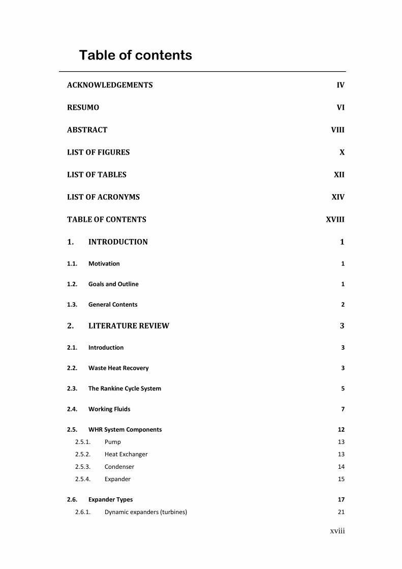
7

the Pinch Point Temperature Difference (PPTD), which should be at least 10 ºC higher

than the inlet working fluid saturation temperature in the heat exchanger, Santos et al.

(2011). The PPTD is the difference between the exhaust gas temperature and the

temperature at which the working fluid begins to vaporize, so it must be considered as the

smallest temperature difference in the heat exchanger, as illustrated in the Figure 2.3.

Figure 2.3 – T-H diagram illustrating the Pinch Point Temperature Difference

(PPTD).

The overall cycle performance is significantly affected by the properties of the

working fluid selected. The next section presents a detailed literature review on the

working fluids that can be used in automotive RC applications.

2.4. Working Fluids

There are several studies on working fluids in order to determine which one suits

best for a determined application. Variables like temperature and pressure have a large

impact on the working fluid properties, and its saturation curves can be depicted in a T-s

diagram. Figure 2.4 shows a representation of the saturation curves in a T-s diagram for

different working fluids: a) isentropic; b) wet; c) dry.

8

Figure 2.4 - T-s diagram for different working fluid types: a) isentropic; b) wet; c)

dry, Santos et al. (2011).

Figure 2.4a) depicts that isentropic fluids have an almost vertical vapor saturation

line (on the expansion side). Wet fluids have a negative slope vapor line and lead to

droplets at the end of the expansion (see Figure 2.4b)), and as a result, they demand

superheating before the expansion process in case of using a turbine, to guarantee that the

expansion process ends outside the wet region. Dry fluids have a positive saturation curve

and the expansion process ends in the superheated vapor region (see Figure 2.4c)),

therefore a recuperator can be used in order to increase cycle efficiency, Santos et al.

(2011), Quoilin et al. (2012), Latz et al. (2012), Latz et al. (2013).

Relatively to the thermodynamic characteristics, it is necessary to analyze the fluid’s

critical point, specific heat, density, etc., in order to determine its suitability. Regarding the

environmental aspects, the values of the Ozone Depleting Potential (ODP) and the Global

Warming Potential (GWP) must be low (particularly the ODP, which is being ruled out

due to the Montreal Protocol, UNEP (1987)). In terms of side effects, flammability and

toxicity must be considered (generally, engine exhaust gases reach about 500ºC, Hamilton

& Hamilton (2015)) and the fluid must be the less toxic possible in case of system leakage.

For the working fluid selection, some criteria should be followed. Starting with the

thermodynamic characteristics, then the environmental aspects and finally the side effects,

it is necessary to fully check all these factors before selecting the appropriate fluid for the

RC system, Quoilin et al. (2012). Thus, fluids with ODP should be excluded from the

beginning because they will be ruled out in the future. The GWP may be considered of

great importance too, but considering that the cycle is closed, this value may only be

considered after a study of the fluids’ Life-Cycle Assessment (LCA).

Some other considerations must be done for the appropriate selection of the correct

working fluid. Organic fluids are more adequate than water for low heat sources due to

lower heat of vaporization, Jadhao et al. (2013). The subcritical or supercritical Rankine

9

cycle has a large impact on the configuration of the physical system, for it may influence

the amount of components required. For example, if a supercritical RC is employed it may

be possible to achieve higher efficiencies without the need of an evaporator because the

fluid is compressed to a pressure above its critical pressure, Latz et al. (2012). However,

supercritical RC systems were disregarded from the present study due to safety issues.

The working fluids mostly considered for application in automotive vehicle WHR

RC systems are showed in Table 2.1.

Table 2.1 - Properties of the working fluids that can be used for RC systems.

- Information not available

Fluids may be categorized by pure (for example, water and ethanol) and mixed

(water-ethanol, R245fa, among others). Mixed fluids can be azeotropic or zeotropic. An

azeotropic fluid is a mixture of two or more fluids with similar boiling points that work as

a single fluid; while a zeotropic fluid has different boiling points in which boiling them

may result in fluid separation. In these mixtures, the boiling point is lower than the boiling

10

point of either substance. In water-ethanol mixture, a mixture with a 95,6% of ethanol and

4,4% of water results in a boiling point of 78,2 ºC, which is 0,3ºC lower than ethanol’s

boiling point and 21,8ºC lower than the water’s boiling point, Latz et al. (2012), Clark

(2005), Imelda (2011).

Teng et al. (2011) developed a Rankine cycle for a 10.8 HD engine, to investigate

the fuel economy benefit. Ethanol was chosen among four working fluids: ethanol, water,

R245fa and 50-50 wt% water-ethanol mixture. Ethanol showed advantages among the

studied fluids because of a condensation pressure higher than 1 bar and evaporation

pressure around 4 bar. Figure 2.5 shows the T-s diagram for the four fluids considered.

Figure 2.5 - T-s diagram of water, ethanol, R245fa and a water-ethanol mixture,

adapted from Teng et al. (2011).

Latz (2013) also studied a system working on a water-ethanol mixture (containing

80% water and 20% ethanol), and found that this mixture is the optimal working fluid,

offering a good trade-off between performance, safety, vehicle applicability, and lack of

environmental issues. Organic fluids like refrigerants either performed poorly under the

studied conditions or, aforementioned, had problems relating to high GWP and safety. In

11

this study, pure water was also excluded as a potential working fluid because it freezes at

relatively high temperatures, as compared to the other working fluids (see Latz (2013)).

Haller et al. (2014) studied two Rankine cycle system arquitectures with two

different expanders and four working fluids in total. In the low temperature (LT) RC

system the fluids used were R134a and R245fa, and the expander selected was a scroll

machine adapted from an air-conditioning system. Water and ethanol were used for the

high temperature (HT) RC system, with a piston machine as expander. It was concluded

that at an ambient temperature of 22°C, R134a or R245fa systems are more powerful than

ethanol system for car velocity respectively less than 120 km/h and 135 km/h.

Panesar et al. (2013a) investigated the application of a RC system as a Bottoming

Cycle (BC) applied in a 10 litre HDD engine for potential improvements in fuel efficiency.

The authors reviewed a fluid selection methodology using seven working fluids: water,

ethanol, R245fa, ethyl-iodide, R1130, R30 and acetone. Authors stated that the molecular

weight of the working fluid has impact on the power required by the pump - fluids with

less molecular weight require less pump power. Also, a fluid with lower Volume Flow

Ratio (VFR) will result in a more compact expansion machine, reducing the system size. It

was concluded that ethanol was the best solution but R1130, acetone and R30 were also

good alternatives.

Seher et al. (2012) tested a RC system in a 12 L HDD and analyzed, by one

dimensional simulation, two expansion machines - turbine and piston - and five working

fluids: water, ethanol, HMDSO (hexamethyldisiloxane), R245fa and toluene. The

boundary conditions at the inlet of the expander were 32 bar of maximum pressure and

380ºC of maximum temperature. The condensation temperatures were set to 100 ºC. For

the turbine expander, all the five fluids were considered, and for the piston, only ethanol

and water. Toluene showed to be the most favorable, but for being classified as harmful for

health, it was not recommended. The organic fluid R245fa showed the lowest performance

on the tested conditions. The work reveals that the best working fluids are ethanol and

water with the piston expander and ethanol with the turbine expander.

Kunte et al. (2013) performed a study on a turbine expander, selecting ethanol

instead of water, isopentane, R245fa and methanol, and limited the cycle to a maximum

temperature of 276,85ºC to avoid ethanol decomposition. The minimum and maximum

operating temperature of the turbine were established to be 70ºC and 256,85 ºC,

12

respectively, with a maximum pressure of 39,8 bar, ensuring a safe operation of the

turbine. Ethanol was selected because it not only showed good behavior in power output,

but also for its high molecular mass. Ethanol has a higher molecular mass than water and

methanol, leading to a lower speed of sound and lower rotational speed of the turbine, for

the same turbine diameter.

Galindo et al. (2015) presents an experimental study on a system that uses ethanol, in

order to test a swash-plate piston expander. The authors claim that ethanol is one of the

best solutions to recover thermal energy in a range of temperatures of 100ºC to 450ºC.

Ethanol is environmental friendly, has high expansion ratios, condensation temperature at

atmospheric pressure, low freezing point and is relatively cheap, with the only downside

being the fact that it is highly flammable.

In resume, the extensive literature survey revealed that the ethanol and water-ethanol

mixtures are the best candidates as working fluids for automotive vehicle RC systems.

Water-ethanol has a good trade-off between performance, safety, vehicle applicability and

lack of environmental issues, and ethanol shows good condensation and evaporation

pressure and has a high molecular weight, which allows lower rotational speed of the

turbine.

2.5. WHR System Components

The rankine cycle system is based in four main components: the pump, heat

exchanger, expander and condenser. The pump raises the pressure of the fluid to a higher

pressure level; the heat exchanger uses the heat from the hot exhaust gases to evaporate the

working fluid, which is expanded in the expansion machine, producing power. The final

step is returning the gaseous fluid into its liquid state, in the condenser.

In automobiles, the system must be compact and light, and for that reason, a single

component has to do all the work for each step. However, some systems may have other

additional components, like subcoolers or safety tanks. The subcooler is usually connected

after the condenser and before the pump, and is used to avoid cavitation. As for the safety

tank, a working fluid reservoir between the condenser and the pump may be used,

preventing the uncondensed vapor from entering the pump.

13

2.5.1. Pump

The pump raises the pressure of the working fluid, between the condenser and the

evaporator. When the compression happens, the fluid is in its liquid state, and with the

fluid in liquid state, pumps can achieve very high efficiencies with high pressure ratios. For

this reason, it has a small impact on the overall performance of the RC system, Lopes et al.

(2012). Many pumps can be found in the market for many applications and different

pressure ratios and fluids for being a widely used and developed technology. The pump

speed shall be variable in order to meet the requirements for working fluid flows at the

different load points.

Teng et al. (2011) used a Vickers VMW double-action 10 cc/rev vane pump, for its

double action feature of this pump minimizes the internal leakage and friction. Besides, it

is a rotary pump without the need of a separate lubrication system and handles cavitation

better than a centrifugal pump.

Tahir et al. (2010) used a Rietschle Thomas 5002F Diaphragm mounted in a low

temperature heat source system running on R245fa. It was displacing 0,140 l/m at a

constant rate, and raising the fluid to a maximum of 2,9 bar at 80ºC. It was concluded that

the pump power consumption was higher than expected (5 kW), lowering the overall

thermal efficiency at around 19%.

Galindo et al. (2015) used a stainless steel plunger pump with direct drive from Cat

Pumps, driven by an electric motor at a maximum of 1725 rpm and a volume flow rate of 7

l/min. The fluid used in the system was ethanol, and the maximum pressure achieved was

24,8 bar. The electrical power consumed by the pump was only 1% of the overall power

balance of the system.

2.5.2. Heat Exchanger

The evaporator heat exchanger, also referred as boiler, is the component where the

working fluid changes its phase from liquid to superheated vapor. Generally, it is a single

part and includes the pre-heater, evaporator and superheater.

The biggest issue of the boiler heat exchanger in automotive use is its size and

weight. It must be compact and light enough and still have good heat transfer

14

characteristics. Endo et al. (2007) developed an evaporator prototype integrated in the

cylinder head, mounted externally to minimize modifications to the engine. Thus, densely

layered multi-plate fins were adopted as heat transfer plates, and integrating the unit in the

cylinder head reduces heat loss and size.

According to Lopes et al. (2012), evaporators can be divided in two main categories:

tubes or plates (see Figure 2.6). Tube evaporators include the use of tubes to conduct and

separate the working fluid from the hot source, in a wide variety of types, configurations

and aspects. As for the plate evaporators, they are configured layers that create several

levels of intermittent cold and hot source passages. Their design has to take into account

the thermal source characteristics: type (liquid, gas, and vapour), relative temperature,

mass flow, density and flow direction. In this study, the volume and cost were taken into

account. Generally, for automotive use, weight may also be considered.

Figure 2.6 - Heat exchanger types: left – shell and tube; right – plate and fin, Lopes et

al. (2012).

2.5.3. Condenser

The condenser works on the same principle as the boiler/heat exchanger, except that

the working fluid is the hot source, and an external source will be the cold source –

ambience air or a refrigeration circuit running on water or other fluid.

15

If air is used as the cold source, the cycle behavior may change if the vehicle is

running in summer or cold winter temperatures, as the temperature difference between cold

and hot sources is lower and the energy to be extracted is lower, Tahir et al. (2010).

If the expansion ends in the superheated vapor zone, condensation gets complicated

and a large condenser may be required, Panesar et al. (2013b).

2.5.4. Expander

The expander is the component where the work output of the cycle is generated. Two

main types of expanders can be distinguished: the dynamic (turbo) and displacement

(volumetric) type, Santos et al. (2011). The working fluid goes in the expander at high

pressure and temperature and is exhausted at low pressure and low temperature, which

means a drop in the specific enthalpy of the working fluid inside the expander. The

enthalpy drop is what the expander converts into work, Panesar et al. (2013b).

The performance of the expander strongly affects the performance of the RC system.

There are many important parameters when selecting an expander such as the isentropic

efficiency, pressure ratio ( ⁄ ) or expansion ratio ( ⁄ ),

power output, lubrication requirements, complexity, rotational speed, dynamic balance,

reliability, and cost. The fluid mass flow rate is also an important parameter for expander

design and will significantly affect its efficiency.

The pressure ratio is the ratio between the pressure at the inlet and at the outlet of the

expander (see equation 3), and it is a reference value for its optimal working conditions.

The importance of this value lies on the fact that a machine is designed for a set of target

operating conditions, which may vary a lot in an automotive RC application, and due to

that the efficiency decreases when the system is running out of the off-design conditions.

Kim et al. (2012) studied the optimization of the designed pressure ratio of two positive

displacement expanders, by varying the vehicle operating conditions, in order to operate in

both under and over-expansion states, concluding that the expansion efficiency decreased

gradually during under-expansion operation, and rapidly during over-expansion operation.

Under-expansion operation means that the design pressure ratio is lower than the operating

pressure ratio, and over-expansion operation is the opposite (see Figure 2.7).

16

Figure 2.7 – Isentropic expansion in PV diagrams: a) under-expansion and b) over-

expansion, Kim et al. (2012).

The isentropic efficiency of an expander is the ratio of the real power output

achieved compared with the theoretical one, and can be calculated as follows:

(3)

The isentropic efficiency ( ) is of major importance for the expansion process and

strongly influences the overall RC system efficiency. Figure 2.8 depicts the expansion

process for both real and isentropic cases: the process 3 to 4s corresponds to an isentropic

expansion, and the process 3 to 4 corresponds to the real process. Point 4 is defined by the

isentropic efficiency of the expander.

Figure 2.8 - Rankine cycle considering both isentropic expansion and real expansion,

Stine & Geyer (2001).

The next section presents a literature review and a detailed explanation on the

different expander types.

17

2.6. Expander Types

The expanders are classified in two main categories: the displacement type

(volumetric) and the dynamic type (turbo), as can be seen in figure Figure 2.9.

Figure 2.9 - Diagram of the various expander types, adapted from Dingel &

Ambrosius (2014).

Displacement type machines are more appropriate for small-scale ORC units,

because they are characterized by lower flow rates, higher pressure ratios and much lower

rotational speeds than turbo-machines. Moreover, these machines can tolerate two-phase

conditions, which may appear at the end of the expansion in some operating conditions,

Lemort et al. (2009). The slow rotational speed of the displacement type expanders makes

them good candidates for direct connection to the engine’s shaft. However, they are

heavier and bulkier than a turbine for the similar conditions, Latz et al. (2013).

On the other hand, turbine expanders achieve much higher rotating speeds than

reciprocating expanders, making them very good in producing electrical power, where the

expander is connected to a generator. There is also the possibility of connecting them to the

engine’s crankshaft, using a gearbox, Santos et al. (2011). However, turbine expanders are

very sensitive to droplets, so they should only be selected in case of dry or isentropic

18

working fluids. If the working fluid is wet (e.g., water), reciprocating expanders are the

most suitable.

Lopes et al. (2012) gathered the results of many studies for each different expander

technology. Table 2.2 shows the values from the previous studies.

Table 2.2 – Values from previous studies found in Lopes et al. (2012).

19

Most of the studies found in Table 2.2 were gathered for low temperature cycles,

which is not adequate for automotive. Seher et al. (2012) studied a system mounted in a

12L HDD engine, using a single-cylinder piston expander. The system data is depicted in

Table 2.3.

Table 2.3 – Compilation of the data of the system found in Seher et al. (2012).

Water Ethanol Unit

Max. temperature of working fluid at

expander intake >400 240 [ºC]

Pressure of working fluid at condenser 1 2,3 [bar]

Maximum pressure of working fluid 40

Expander displacement 0,9 [L]

Expander Stroke 81 [mm]

Piston diameter 87

Bosch (2012) provides data for the technical features for the WHR system, for the

piston machine (also available in Seher et al. (2012)) and for the turbine expander

machine. The features can be seen in Table 2.4.

Table 2.4 - Technical features of WHR system applied to a HDD engine, Bosch (2012).

System

Type RC system

Thermal Input 100 – 300 [kW]

Fuel Savings around 5%

Lifetime 1,6 Million km

Expanders

Type

Piston Machine Turbine with transmission

Single cylinder

double-acting Constant pressure turbine

Displacement 0,9 [L] -

Mass (total) around 40 kg around 25 kg

Max Power 25 [kW]

Max Temperature 300 [ºC]

Max. Pressure 50 [bar]

Power Take-off Crankshaft via

clutch, gear drive

Crankshaft via

transmission and clutch,

gear drive or generator

20

Latz (2013) performed a dimensionless analysis in two classes of expansion devices:

displacement expanders and turbine expanders. The author uses the volume flow rate and

the isentropic enthalpy drop of the working fluid over the expander as input variables. It

was concluded that displacement expanders offered the highest thermal efficiencies when

using a high expansion pressure ratio with a water-alcohol mixture as the working fluid.

However, acceptable efficiencies could be achieved with single-stage turbine expanders by

reducing the expansion pressure ratio and using an organic working fluid, both of which

would increase the mass flow rate through the system.

From a thermodynamic point of view, the Rankine cycle is more efficient at high

expansion pressure ratios. It would therefore be desirable to develop single-stage turbines

that allow the use of high expansion ratios or compact multi-stage turbines, both of which

would be easier to integrate into small vehicles compared to a more bulky displacement

expander. However, in a previous study, Latz et al. (2013) states that multi-staged turbines

increase their cost and complexity, which may be proved as an unsuccessful solution.

Table 2.5 presents a resume of the expander types investigated in previous studies.

Table 2.5 - Resume of the expander types investigated in previous studies.

Dynamic (turbo)

Radial Turbine (Seher et al. 2012)

Axial Turbine (Seher et al. 2012) (Kunte et al. 2013) (Dingel &

Ambrosius 2014)

Mixed Flow Turbine (Seher et al. 2012)

Displacement (volumetric)

Rotary Vane (Lopes et al. 2012) (Tahir et al. 2010)

Scroll (Lopes et al. 2012) (Lemort 2013) (Legros et al. 2014)

(Lopes et al. 2012) (Lemort et al. 2009)

Screw (Lemort 2013) (Legros et al. 2014)

Piston

(Seher et al. 2012) (Lopes et al. 2012) (Lemort 2013)

(Legros et al. 2014) (Glavatskaya et al. 2012) (Berger

2014)

Swash-plate Piston (Endo et al. 2007) (Lopes et al. 2012) (Kim et al. 2012)

21

2.6.1. Dynamic expanders (turbines)

Turbo-expanders operation is based on the high-pressure gas being directed past the

turbine blades causing them to rotate as the gas expands. As stated before, turbines can be

axial, radial or mixed flow, depending on the inlet flow direction. Figure 2.10 shows a cut-

view of a turbine expander.

Figure 2.10 – Cut-view of a Turbine Expander, Lopes et al. (2012).

Turbine expanders operate at high rotating speeds (50000 rpm can be easily

achieved, Panesar et al. (2013a), but can go up to 160000 rpm, Kunte et al. (2013), making

them preferable to use in converting the energy to electricity.

Lopes et al. (2012) state that the most critical factor for high performance turbine

expanders is be the blade speed ratio, given by the ratio between tip speed (U), and the

isentropic spouting velocity (C), and that the optimal value for a radial turbine in a small-

scale installation is 0,7 (velocity ratio, see eq. 4). Santos et al. (2011) state that the high

speed of turbines is related to the blade Reynolds number (see eq. 5) and that this value

should be on the order of , and also recommend a Mach number (see eq. 6) of 0,85 to

avoid local choking on the flow rotor.

(4)

22

(5)

(6)

In eq. 5, is the rotary speed of the blade, is the diameter of the rotor and is the

fluid’s kinematic viscosity. In eq. 6, is the velocity on the tip of the blade and is the

speed of sound.

As compared to other working fluids (like water) ethanol has a high molecular mass,

leading to a lower speed of sound and as a result to a lower rotational speed of the turbine

for the same turbine diameter.

According to Sauret & Rowlands (2011), that studied turbine expanders for

geothermal applications, the author states that axial turbines handle higher flow rates than

radial turbines, but radial turbines achieve higher pressure ratios. Also, from a mechanical

point of view, radial inflow turbines are less sensitive to blade inaccuracies than axial

turbines, maintaining high efficiencies as size decreases. They are also more robust under

increased blade load using high density fluids, at both subcritical and supercritical

conditions, and have higher stiffness, which improves rotor-dynamic stability of the system

and makes them easier to manufacture because the blades are attached to the hub.

In resume, for small-scale applications, turbines must rotate at very high speeds in

order to maintain optimal performance, single-stage turbines have low pressure ratios and

they have shown to have isentropic efficiencies up to 85%. Also, if the expansion ratio is

smaller than 50, they can achieve isentropic efficiencies higher than 0,8 with single stage

only, Santos et al. (2011). They are precision machines that are expensive. The solution to

round the low pressure ratio problem is to select multiple-stage turbines, which increases

even more their cost.

23

2.6.2. Displacement expanders (volumetric)

The majority of the RC systems under research for automotive applications employ

positive displacement machines, Lopes et al. (2012). Positive displacement expanders

differ from the turbine expanders in the fact that they have a volume chamber, which limits

the volume of the fluid inside the machine with each revolution.

2.6.2.1. Rotary vane expander

Rotary vane expander machines consist in a housing with inlet and exhaust, a rotor

with vane slots and the vanes, and operate by the inlet of high temperature and pressure

vapor that by expansion cause the rotor to move, which in turn increases the expansion

volume. At the end of the expansion, the vapor is exhausted. Figure 2.11 shows the

operation of the rotary vane expander.

Figure 2.11 - Vane expanders operation. 1 – intake, 2 and 3 – expansion, 4 – exhaust,

Lopes et al. (2012).

With the expansion process, the vanes are kept in contact with the housing by the

means of springs or magnetic force, sealing the different volumes and isolating them.

These type of expanders need lubrication and may suffer pressure drops of 65% and losses

of 20% caused by leakages, due to the inability of the vanes to maintain a regular contact

pressure against the housing, Lopes et al. (2012). Also, at higher speeds, frictional losses

become more important, and high pressures may make the vanes bounce and strike against

24

the cylinder wall, reducing expander’s life and performance, Lopes et al. (2012). They are

tolerant to wet expansion and have a simple mechanism and minimal mechanical parts,

which makes them very cheap, Santos et al. (2011).

2.6.2.2. Scroll expander

Scroll machines can be found in a large scale in the market as compressor machines.

Besides, scroll air compressors may easily be adapted to work as expansion machines for

testing purposes. It only has one moving part and consists in two spirals, one moving in

eccentric circles and one stationary. The fluid goes in through an orifice in the center of the

spiral and gets transported to the side, expanding on the way and consequently rotating the

spirals.

Scroll expanders can be categorized in two types: compliant and constrained, Lopes

et al. (2012). A compliant scroll requires lubrication and uses the centrifugal effect to keep

the orbiting scroll in continuous contact with the fixed scroll, and a constrained scroll can

operate without lubrication and be constrained either radially, axially or both. Their

manufacturing tolerance must be considered as a critical parameter in case of a constrained

type, having higher leakages and friction losses than a compliant type. The presence of oil

inside the expander is a problem of big importance because it may mix with the working

fluid inside the scroll, changing its properties. Also, there is the problem of radial leakages

and friction losses, which cause poor performance, Lopes et al. (2012). The maximum

internal built-in volume ratio is usually inferior to 5, Santos et al. (2011), Lemort (2013).

The built-in volume ratio corresponds to the displacement volume of the expander

machine. Figure 2.12 shows the two main leakage types in a scroll expander.

25

Figure 2.12 - Two main leakage types in a scroll expander, Lopes et al. (2012).

The displacement volume of scroll expanders usually varies between 1,1 l/s to 49 l/s

and the rotational speed values can range between 1000 rpm and 4000 rpm (see Table 2.2).

Built-in volume ratio is generally between 1,5 and 3,5, because higher values can cause

sealing problems. The pressure ratio of scroll machines for expander operation may be up

to 15, and selecting this type of expander for high discharge temperature applications is not

recommended, the high temperature operation can cause degradation of the lubricant oil.

Maximum operating temperatures of 165 and 215ºC for air and steam (respectively) were

achieved in previous studies, Legros et al. (2014).

Kim et al. (2012) used a scroll expander with a displacement of 40 and a rated

driving speed of 3600 rpm in the study for the low temperature RC system (see Figure

2.13).

Figure 2.13 - Scroll expander used in the LT cycle by Kim et al. (2012).

26

2.6.2.3. Screw expander

Screw expanders operate by inletting the working fluid on the intake side, trapping

the fluid between the blades and the housing as it moves forward, which expands and

rotates the screws on the way to the exhaust side. The fluid is then expelled through the

exhaust.

Figure 2.14 - Twin Screw Expander, Langson (2008).

The power range of screw machines is between 20 kWe and 1 MWe with

displacement volumes going from 25 l/s to 1100 l/s. They can achieve high rotational

speeds (up to 25000 rpm), can be synchronized or unsynchronized and require lubrication.

The typical built-in volume ratio is around 5 and they can tolerate high temperatures

(490ºC) and high pressure ratios (Nikolov et al. (2012) considered a value of 50 with

ethanol). Screw type compressors are widely found in the market. For instance, they are

commonly used in automobiles and heavy duty industrial machinery as superchargers.

Small screw machines can compete with big scrolls, and their only moving parts are the

screws. Screw type expanders can be found in geothermal systems running on steam,

Lopes et al. (2012). The main drawback is the manufacturing precision required, especially

in the synchronized ones.

This type of expander is a good solution for heavy industrial systems. Nevertheless,

for automotive vehicles, screw expanders are turned down because of their size, weight

and power.

27

2.6.2.4. Piston

Piston machines work according to the same principle as reciprocating ICEs, based

in four main processes – intake, compression, power and exhaust (Figure 2.15).

Figure 2.15 – Piston expander machine – working principle.

For ICEs four stroke engine, the intake process occurs while the piston is moving

down inside the cylinder. When it starts moving back up, the intake valve closes the

compression process occurs. Then, after reaching the top of the cylinder, the combustion

occurs and the piston is forced down (power). Finally, after reaching the bottom, the

exhaust valve opens and the resulting combustion gas exits the cylinder.

As expansion machines, the working principle is the same, but the inlet and

expansion occur simultaneously, and the expansion is independent (Figure 2.16).

Figure 2.16 – Piston expander machine working principle, Lopes et al. (2012).

28

The first process (intake and expansion) occurs with the exhaust valve closed. The

piston is at the top of the cylinder and the inlet valve opens, letting the high pressure and

high temperature fluid enter de cylinder, and driving the piston down in the process. When

the piston reaches the bottom, the inlet valve closes and the outlet valve opens, letting the

working fluid (now with lower pressure and low temperature) exit the cylinder, while the

piston moves upwards. After the piston reaches the top of the cylinder, the cycle begins

again.

The inlet valve can be rotating, sliding or poppet, and for the exhaust, there can be

either valves or ports, Lemort (2013). Figure 2.17 show both the real and ideal PV diagram

and the valve lift diagram of a typical piston machine.

Figure 2.17 – Piston machine diagrams - Top Left: Real PV; Top Right: Ideal PV,

Wikipedia (n.d.); Bottom: Valve Lift.

29

The reciprocating-type expander seems to be considered more appropriate for

combining mechanical energy output directly to the crankshaft, in particular for on-road

vehicle applications where the condition for waste heat is variable, because of its

flexibility, Lopes et al. (2012). When compared to scroll and rotary vane expanders, they

are preferred because they are suitable for higher pressure ratios, which allows a better

efficiency of the global RC system, Galindo et al. (2015). They have high resistance to

water droplets, tolerate high working fluid pressures and work well under large volume

ratios. The drawbacks are the friction losses at higher pressures and possible sealing

problems on the piston contact with the cylinder wall, Santos et al. (2011).

Built-in volume ratios between 6 and 14 are usually achieved for piston expanders,

thus they tolerate large pressure ratios. The volume displacement of typical reciprocating-

type expanders ranges from 1,25 l/s to 75 l/s, Lemort (2013). The rotational speed is

similar to that achieved by ICE’s. Temperatures can go up to 500ºC and pressure ratios

relatively similar to ICE’s, according to Legros et al. (2014). Piston expanders from

EXOES (2011) achieve speeds between 500 and 6000 rpm.

2.6.2.5. Swash-plate piston expander

The present work considers a swash-plate expander type, which is also in the

category of the piston expanders.

Galindo et al. (2015) claim that the swash-plate piston expanders are increasingly

taking into account among the reciprocating type due to their versatility, compactness,

robustness and good specific power.

Endo et al. (2007) studied a system in a swash-plate piston expander (see Figure

2.18), with 7 cylinders, a geometric expansion ratio of 14,7 and a maximum rotating speed

of 3000 rpm. The expander allows a maximum temperature of 500ºC and pressure of 90

bar. The application of a RC system using a swash-plate piston expander allowed the

thermal efficiency of the base vehicle to increase from 28,9% to 32,7%, which means a

13.2% relative increase.

30

Figure 2.18 - Swash plate piston expander from Endo et at. (2007).

Kim et al. (2012) also used a swash-plate piston expander for their high temperature

(HT) cycle. The expander had 5 cylinders, a piston diameter of 30 mm, a displacement of

108 , and a rated driving speed of 2450 rpm (see Figure 2.19).

Figure 2.19 - Swash plate piston expander used by Kim et al. (2012).

31

3. Expander Selection

3.1. Introduction

The previous chapter provides a detailed review on the different types of expanders

that can be used in RC systems for automotive application. This chapter is dedicated to the

expander selection. To this end, the selection parameters and methodology applied for the

expander selection are explained.

This chapter starts with the parameters used to select an expander machine and

describes the NsDs turbine chart. A detailed explanation of the steps required to obtain the

points in the chart will be given and a verification of the methodology using 3 different

working fluids will then be performed.

3.2. Selection parameters

The waste heat provided by an automotive vehicle varies accordingly to the ICE’s

operating conditions, so a RC system designed to work under a certain target operating

condition will sometimes operate under off-design conditions, and so that the pressure ratio

is strongly affected with these constantly varying conditions. Kim et al. (2012) studied a

dual loop system solution in order to avoid this problem, using a HT (high temperature)

cycle with a swash plate piston expander and a LT (low-temperature) cycle with a scroll

expander, covering both high and low heat sources and optimizing the overall working

conditions of the cycle. It was concluded that for both cycles, with only a decrease in

around 7% of the expansion efficiency, the weight and volume of the expanders would be

decreased in approximately 39% for the HT cycle and 33% for the LT cycle.

The company Barber-Nichols proposed a NsDs chart that allows to select the optimal

expander type as a function of the dimensionless parameters: specific speed (Ns) and

specific diameter (Ds) for each use case. Figure 3.1 depicts the NsDs turbine chart. It is

based on a similarity concept that states that the number of parameters describing the

characteristics of an expansion machine can be reduced to four dimensionless numbers: i)

the Mach number ( ); ii) the Reynolds number ( ) at the inlet of the expander (which

32

have secondary effects on the expander’s behavior); iii) the specific speed ( ) and iv) the

specific diameter , Keneth (1959), Latz et al. (2013), Sauret & Rowlands (2011). The

eq. 7 and eq. 8 allow the calculation of the specific speed ( ) and the specific

diameter :

√

⁄ (7)

⁄

√

(8)

In the eq. 7, is the rotating speed [rpm] and is the volumetric flow rate at

the expander outlet [ ⁄ ]. In the eq. 8, is the diameter [ ]. In both equations, is

the specific enthalpy drop in height of fluid [ ].

Figure 3.1 - Barber Nichols "how to select turbomachinery for your application",

Keneth (1959).

In addition to the Barber Nichols turbine chart, the Figure 3.2 and Figure 3.3 show

the Dixon’s turbine chart and the Japikse’s expander machine solution chart, respectively,

Sauret & Rowlands (2011). The Dixon’s turbine chart is used specifically for turbine type

expanders and the Japikse’s expander machine selection chart is for any expander type.

Barber Nichols’ chart uses imperial units and Dixon’s chart uses metric units. The other

input of the Dixon’s chart is the overall efficiency of the turbine ( ), as can be seen in

Figure 3.2.

33

Figure 3.2 – Dixon’s turbine chart (adapted from Dixon (1977)).

The specific speed ( ) in Figure 3.2 is calculated through eq. 9:

⁄

⁄ (9)

In eq. 9, is the rotary speed [rad/s], Q is the volumetric flow rate [ ⁄ ], g is the

acceleration of gravity [ ⁄ ] and H is the head of fluid [m].

For Japikse’s chart, the inputs are the flow coefficient ( ), the head coefficient ( )

and the specific speed ( ). The calculations required for the Japikse’s chart are in metric

units. The chart is presented in Figure 3.3.

Figure 3.3 – Japikse’s expander machine selection chart (adapted from Sauret &

Rowlands (2011)).

34

Eq. 10, 11 and 12 are used as inputs in the graph of the Figure 3.3.

( )

(10)

(11)

(12)

In eq. 10, is the dimensionless flow coefficient, is the inlet volume flow rate

[ ⁄ ], is the speed at the outlet of the expander [ ⁄ ] and is the diameter of the

expander [m] (in case it is a turbine, D is the diameter of the outlet rotor). Eq. 11 stands for

the head coefficient ( ), where is the variation of the height of fluid [m] and is the

speed of the fluid at the inlet of the expander [ ⁄ ]. In eq. 12, is expressed in [ ⁄ ].

The detailed explanation of the equations can be found in Dixon (1977).

The values obtained for each chart are different for the same type of machine.

According to Sauret & Rowlands (2011), for radial-inflow-turbine expanders, the typical

values for the specific speed should be: i) between 30 and 100 for the Barber Nichols’s

chart; ii) between 0,1 and 1 in the Japikse’s chart and iii) 0,5 and 0,9 in the Dixon’s chart.

For this work, the chart used for the machine selection is the Barber Nichols, in

imperial units.

3.3. Methodology

The working fluid operating conditions at the expander inlet depends on the

evaporator (boiler) operating conditions. Therefore, with the working fluid conditions at

the inlet of the expander already determined by the working fluid conditions at inlet and

outlet of the evaporator, as well as its thermal power, it is possible to determine the

working fluid mass flow rate in the RC system, which is important to define the parameters

required for the expander selection using the NsDs expander chart. Figure 3.4 shows a

diagram of a step-by-step methodology for the determination of the points for the NsDs

expander chart, and consequently the type of expander for a specific application.

35

Figure 3.4 – Diagram that describes the sequence used to calculate de Ns and Ds

parameters.

Initially, the pressure and temperature at the inlet of the evaporator ( ; ) and at the

evaporator outlet ( ; ) are defined, and using the REFPROP, Lemmon et al. (2010),

EES, FChart (n.d.), or other similar thermodynamic software, the enthalpies ( ) and

the entropy ( ) are determined. Note that the state 3 corresponds to the inlet of the

expander, considering that the ducts are short and will not have great influence in the

theoretical calculations.

36

Another value given initially is the power of the evaporator ( , and with the

inlet and outlet enthalpies obtained in last step, the mass flow rate of the working fluid can

be calculated using eq. 13. Also, having the pressure at the inlet of the expander ( ) and

the pressure at the outlet of the expander ( ), the pressure ratio (Π) can then be calculated

through eq. 14.

(13)

(14)

The step is determining the isentropic enthalpy at the expander outlet. For that, the

isentropic entropy ( ) is needed. For the isentropic expander process the entropy at the

outlet of the expander ( ) is equal to the entropy at the inlet ( ). The isentropic enthalpy

( ) can then be calculated accordingly, using the pressure at the outlet of the expander

( ) and the isentropic entropy ( ) as reference values.

Using the isentropic efficiency definition, the enthalpy at the outlet of the expander

( ) can be calculated as follows:

(15)

After that, by using the pressure ( ) and the enthalpy ( ) at the outlet of the

expander the state 4 is defined and as a result, the remaining thermodynamic properties

(such as , and ) can be obtained.

Next step is calculating both the height of fluid ( ) and the volume flow rate ( ),

using equations 16 and 17, respectively.

(16)

(17)

In eq. 16, is the head of the fluid [m], is the enthalpy [ ⁄ ] and g is the

gravitational acceleration [ ⁄ ]. In eq. 17, is the volumetric flow rate [ ⁄ ], is the

mass flow rate [ ⁄ ] and is the density of the fluid [ ⁄ ].

37

To calculate the specific speed ( ) and the specific diameter ( ), the head of fluid

( ), the volumetric flow rate ( ) and the diameter (D) must be converted from SI units to

Imperial units, using the conversions (

).

3.4. Selection of an expander for an

automotive RC system

For automotive vehicles RC system application, the evaporator works in a power

range between 10 kW and 500 kW. The corresponding working fluid mass flow rate is

calculated through eq. 11. To that, for each working fluid evaluated (R245fa, ethanol and

water), a minimum and a maximum mass flow rate will be calculated. From this will result

a region in the NsDs expander chart limited by the two corresponding NsDs points

obtained, one minimum and one maximum.

Such as already referred three fluids were used for the present study analysis:

R245fa, ethanol and water. Ethanol and R245fa were selected because of the potential

showed in previous studies for small-scale RC applications, Panesar et al. (2013b), Wang

et al. (2011), and water was selected for comparative reasons for it is a non-flammable and

non-toxic fluid and is used for many energy recovery systems, Lopes et al. (2012), Panesar

et al. (2013b).

Figure 3.1 shows a diagram with the working fluid properties used to start the

calculations, according to the point in the system and the working fluid in use.

38

Figure 3.5 – Diagram of the process and initial values for calculations.

The pressure at the inlet and outlet of the evaporator are equal (isobaric process), so

it will be named as evaporation pressure ( ), and the pressure at point 4 will be named

as condensation pressure ( ). Table 3.1 resumes the properties for each working fluid.

Table 3.1 – Resume of the thermodynamic properties.

[ ] [ºC] [ ] [ºC]

R245fa 50 150 12 97,657 4 54,995

Ethanol 80 240 20 180,42 2,5 103,08

Water 80 300 20 212,38 1 99,6

Speed and diameter of the expander were selected according to previous studies, for

both displacement and turbine expander machines, Lopes et al. (2012), Galindo et al.

(2015), Declaye et al. (2013). For the diameter and rotational speed of the expanders, the

literature review demonstrated that a value of 0,03 [m] for the diameter was appropriate for

the calculations, and that for the rotational speeds, more values should be tested in order to

cover the range studied in previous works, Kunte et al. (2013), Kim et al. (2012), Lemort

39

et al. (2009), Lopes et al. (2012), Endo et al. (2007). Six different test conditions will be

performed for the three different working fluids (see Table 3.2). Considering the test

conditions in the Table 3.2, the test conditions 1, 2 and 3 represent rotational speeds that

are suitable for displacement expanders (1000 rpm to 3000 rpm), and the test conditions 4,

5 and 6 correspond to rotational speeds suitable for turbine expanders (20000 rpm to 10000

rpm).

Table 3.2 – Rotary speeds used for calculations.

Test

Condition

Speed Diameter

[rpm] [m]

Displacement

Expanders

1 1000

0,03 2 3000

3 5000

Turbine

Expanders

4 20000

0,03 5 50000

6 100000

Table 3.3 presents a resume of the input parameters used in the calculations. Two

mass flow rates were calculated according to the minimum and maximum limits chosen for

the evaporator (10 kW and 500 kW) for automotive applications. The higher the evaporator

power, the higher the mass flow rate obtained.

Table 3.3 – Excel table with the thermodynamic inputs.

40

Considering the evaporator thermal power in the range 10 kW to 500 kW and the

working fluid operating conditions (see Table 3.1), the working fluid mass flow rate ranges

from: i) 30,63 g/s to 1531,4 g/s for R245fa; ii) 8,28 g/s to 414,18 g/s for ethanol and iii)

3,72 g/s to 186,04 g/s for water. Considering the evaporator and condenser pressures, the

pressure ratio (PR) is: 3 for R245fa, 8 for ethanol and 20 for water.

Table 3.4 shows the input values for the expander and also the resultant specific

speed ( ) and specific diameter ( ). The minimum value of each fluid corresponds to the

minimum (10 kW), and the maximum (500 kW) evaporator power.

Table 3.4 – Excel table with the values for the expander and the resultant specific

speed and specific diameter (test condition 1, see Table 3.2).

The results obtained for the test points for displacement expanders displayed in

Table 3.2 are represented in the charts in Figure 3.6 for displacement expanders and Figure

3.7 for turbine expanders.

41

Figure 3.6 – Top: Test condition 1; Center: Test condition 2; Bottom: Test condition 3

(see Table 3.2), corresponding to the displacement expanders rotary speeds and a

diameter of 0,03 m.

42

Figure 3.7 – Top: Test condition 4; Center: Test condition 5; Bottom: Test condition 6

(see Table 3.2), corresponding to the turbine expanders rotary speeds and a diameter

of 0,03 m.

43

The points obtained in Figure 3.6 and Figure 3.7 show that a higher evaporator

power is associated with a larger expander, and that a low evaporator power is associated

with a smaller expander diameter. This also means that higher mass flow rates require

bigger expanders, and lower flow rates require more compact expanders.

From Figure 3.6 and Figure 3.7 it is possible to observe that for the given diameter

of 0,03 m, only test conditions 5 and 6 are obtained inside an expander type region – which

means that for the given diameter, only turbines working under high rotational speeds

should be selected. Besides, only in point 6 all the 3 fluids are simultaneously inside that

area, as for point 5 only R245fa is inside the turbine region. In point 4, raising the

rotational speed to a slightly higher value may result in that the point is obtained inside the

turbine region.

3.4.1. Influence of the expander’s diameter

To evaluate the influence of the expander diameter on the NsDs expander chart, it

was tested an expander used by the authors Daccord et al. (2014) that has a piston diameter

of 160 mm (0,160 m). Note that, the expander diameter used in the selection procedure

presented in the previous section has 0,03 m (see Table 3.2). As a result, the and

values will be recalculated using this diameter value (0,16 m) to determine the influence it

has in the expander NsDs chart. The results are shown in the Appendix 1.

The figures in the Appendix 1 show that a bigger diameter makes the displacement

expanders suitable for selection for the given conditions. In point 1, all 3 fluids are a good

solution, especially for lower evaporator power (the points closer to the expander region

where obtained with the lowest evaporator power of 10 kW), while in point 2 they are all

suitable for a higher evaporator power (closer points were obtained with 500 kW). As for

point 3, water and ethanol still are good solutions if combined with displacement

expanders, while R245fa already reveals a better combination with turbine expanders. Both

points 4 and 5 show that all fluids are suitable for a turbine expander for the tested

conditions, and the same happens in point 6 for high evaporator powers.

44

3.4.2. Expander selection for the present study

The expander used in the experimental setup used for this study was a swash-plate

piston expander, and the setup information can be found in Galindo et al. (2015). The

suitability of the expander in this experimental setup will be verified in this section, and the

points studied are depicted in Table 3.5, Galindo et al. (2015).

Table 3.5 - ORC operating points for simulation in Galindo et al. (2015).

Unit OP 1 OP 2 OP 3 OP 4 OP 5

Boiler Power [kW] 5 12 20 25 30

High Pressure

(evaporator) [bar]

14,8 15,7 18,7 24 24,8

Low Pressure

(condenser) 2,3 1,9 2 2,5 2,5

Mass flow rate [kg/h] 16,67 39,95 64,95 82,01 102,87

Expander Speed [rpm] 1018 2527 3511 3021 3354

Expander Torque [Nm] 2 2,7 3,5 5 5,2

Expander Power [kW] 0,21 0,71 1,28 1,58 1,83

The boiler power was not considered for each point individually. The calculations

were performed considering a boiler power between a minimum of 5 kW and a maximum

of 30 kW for all points, which will result in a region covered by the same point. The results

are presented in the Figure 3.8 and Figure 3.9.

45

Figure 3.8 - Region obtained from the experimental data in the NsDs chart.

Figure 3.9 – Zoom of the region obtained in the NsDs chart from the experimental

data.

The region obtained confirms that a piston machine is the best type of expander for

the experimental setup, for the given conditions. All the five operating points cover the

piston expander region, for the given system characteristics.

46

3.5. Summary

The results confirm the accuracy of the calculations, since the regions obtained in

the charts match the expanders previously selected. One of the conclusions that can be

taken beforehand is that the NsDs expander chart may be used to find the adequate

expansion machine for a given application according to the region obtained, and not a

specific application point. This is due to the proximity of the obtained points and the fact

that the chart has logarithmic scales in both axis, which combined make the results

inaccurate.

Obtaining a region inside a type of expander in the chart means that that type of

expander is the most suitable for that given application. The combination of the with

the results in that a lower diameter of the expander will have to be combined with an

increase in the expander rotational speed, and for low speeds the diameter will have to be

bigger. This means that high speeds and low diameters will mostly result in the turbine

region and low speeds combined with higher diameters will result in the displacement

expander area. Given this, it can be confirmed that turbine expanders are more compact

than displacement expanders.

The expander selected for the experimental setup, Galindo et al. (2015) was a

swash-plate piston expander. According to the calculations performed in this chapter, the

most suitable expander type for the system is a piston expander, which means that the

expander in use is adequate.

An important observation is also the fact that the working fluids’ influence in the

region is not actually very significant, but the R245fa is positioned at the right of the other

fluids in the chart for low speeds, which means that is closer to the turbine region than

water or ethanol – from the 3 fluids, it is the only one suitable for using in combination

with turbines for being a dry fluid. This conclusion is important to the fact that combining

a fluid with an expander must not be done only according to the characteristics of the

system and the NsDs chart, but also according to the characteristics of the fluid and how

they may affect the reliability of the expander selected.

47

4. The expander model

4.1. Introduction

The expander model was developed and validated against experimental data obtained

at the Centro de Motores Térmicos (CMT) of the Polytechnic University of Valencia. The

experimental setup can be found in Galindo et al. (2015). The goal is to obtain results as

close as possible to the experimental runs in order to avoid the expensive and long runs in

the future.

First in this chapter, in section 4.2, there will be a description of the schematic

models found in literature, in order to have a theoretical approach to the model developed.

Then, in section 4.3, information will be provided about the available softwares that are

commonly used in the section as well as their main characteristics. Section 4.4 contains the

description of the final model and the assumptions made. There is a step-by-step

explanation and then a detailed model description, with all the main components explained.

Section 4.5 provides the input parameters that can be already added to the software, taking

into account that most of the values are given by the final results of the experimental runs.

Finally, in section 4.6, the model is validated.

4.2. Different model types

Three types of models can be distinguished: empirical (black-box); semi-empirical

(grey-box); deterministic (white-box), Lemort (2013). An empirical (black-box) model is

characterized by very low computational time and high numerical robustness, does not

allow extrapolation beyond calibration range and is suitable for dynamic simulations of RC

systems. In resume, this model allows to simulate the expander as a black box with specific

boundary conditions at the inlet and outlet. A semi-empirical model is usually used for

steady state simulations, and allows the variation of the operating conditions and

mechanical characteristics due to the fact that those conditions are known, such as: supply

and exhaust pressure losses, internal leakages, mechanical losses, heat losses to the

ambient and under and over expansion or compression losses. A deterministic model goes

48

even further and describes the expander with differential equations of conservation of mass

and energy, and is used for optimizing the expander’s design.

A semi-empirical model on a reciprocating expander was developed by Glavatskaya

et al. (2012). The schematic representation of the model can be seen in Figure 4.1.

Figure 4.1 - Schematic representation of the expander model found in Glavatskaya et

al.( 2012).

In the schematic representation depicted in Figure 4.1, all the steps through which the

fluid goes from the inlet to the outlet of the expander are represented, and the steps are:

- corresponds to the pressure loss that occurs during the suction

process;

- corresponds to the cooling process that occurs by the contact

of the working fluid with the metal housing;

- represents de expansion process, considering an isentropic expansion

( and an expansion at constant machine volume ( );

- represents de compression of the residual working fluid mass trapped inside

the cylinders at the end of the discharge process;

49

- corresponds to the pressure loss at the exhaust of the

expander;

- corresponds to the heating that occurs by the contact of the

cooled working fluid with the heated housing;

- corresponds to the mechanical losses;

- corresponds to the heat losses from the system to the ambient air.

A more detailed explanation of the scheme and all the variables can be found in

literature Glavatskaya et al. (2012), Lemort (2013).

Due to the impossibility of determining the thermal losses, pressure losses and

mechanical losses separately, as well as the residual fluid left in the chamber that will also

cause a loss in the compression process, the model developed in the present work will be

empirical (black-box). All the parameters known for modelling the expander are external

to the box depicted in the Figure 4.2 that presents the inlet and outlet working fluid

conditions, rotary speed, volume of the cylinders and opening and closing angles of the

valve and port.

Figure 4.2 – Empirical (black-box) model of the expander modeled for this work.

50

4.3. Softwares available

Table 4.1 shows a summary of the main softwares used in previous similar studies

and their usage in each study.

Table 4.1 – Softwares used by authors in previous studies.

Software Type of study Authors

EES

- Semi-empirical simulation models

of 3 different expansion machines Legros et al. (2014)

- Steady-state semi-empirical model

of an expander device Glavatskaya et al. (2012)

EES and F-

Chart

Software

- Model for a binary power cycle

considering realistic condensing ORC

cycles for geothermal applications

Sauret & Rowlands (2011)

REFPROP - Fluid properties calculator

Wang et al. (2011),

Arunachalam et al. (2012),

Legros et al. (2013),

Katsanos et al. (2010)

AMESim

- Development ORC simulation

model Ziviani et al. (2012)

- Swash-plate pump detailed model

and simulation Drupal & Nupet (n.d.)

Matlab - Model development

Wang et al. (2011), (Legros

et al. (2013)

- Numerical solutions and graphs Grip (2009)

Other (Non

Specified)

- Turbine and double action piston

machine models using a commercial 1D-

system simulation tool

Seher et al. (2012)

- CAD model of a prototype of a

single-stage impulse turbine of realistic

size and weight

Kunte et al. (2013)

51

The Engineering Equation Solver (EES) is a very powerful tool in terms of

thermodynamic properties calculation and prediction as it provides a very complete

database of fluid properties, making it easy to use by just input the equations and the

values required to compute the solution. It also gives the possibility of drawing parametric

tables in order to obtain various results for different system conditions, so that graphics and

maps can be obtained for a great number of different machines and working fluids. Legros

et al. (2014) used the EES to model, simulate and compare 3 different expanders.

REFPROP (Reference Fluid Thermodynamic and Transport Properties Database) is

also a very complete thermodynamic properties calculator, and was developed by the

National Institute of Standards and Technology (NIST) of the United States of America. It

can be used to calculate the properties of several working fluids, and can also be

interfaced with other softwares, for example Matlab, Wang et al. (2011) or, in the case of

this work, Excel (chapter 3).

LMS Imagine AMESim (Advanced Modeling Environment Simulator) was the

software used in the present work, is a very complete engineering software, with an

extended library, also including an extreme list of working fluids, that can be used to

model several different systems (form small air-conditioning components to complex

mechatronic systems). It allows the simulation of systems under transient and stationary

operating conditions, with specified control strategies. It is adequate for ORC system

modeling and simulation, and for these reasons it was chosen for the present work.

Matlab is a numerical computing environment and a programming language. It can

be used to compute the pressure-volume (PV) diagrams, from the data obtained

experimentally, and to compare it to the diagrams obtained from the AMESim model. It

was used in this work to compare the PV diagrams obtained experimentally with the PV

diagrams obtained with AMESim, in order to adjust and calibrate the model, and also to

determine the accuracy error of the model.

4.4. LMS Imagine AMESim

AMESim is a 1D (one-dimensional) software that allows simulations of various

engineering systems. It is based on an intuitive graphical user interface in which the system

is displayed throughout the simulation process. The model is implemented by connecting

52

the components, in order to model the desired engineering system. The components are

represented through standard symbols used in the engineering field (such as ISO). In the

case that such standards don’t exist, the components are displayed through a pictorial

representation that is easily recognizable by the user. Each component has a number of

ports for connection between them, and when a connection is not possible, the software

blocks the connection, making it also user friendly in saving time in finding errors in the

system connections.

The software AMESim is a very powerful tool that can replace the long and

expensive experimental runs of complex systems, with accuracy and precision, in order to

optimize the overall system, or to optimize some specific parts or components.

The wide range of libraries, divided in a large amount of categories, gives the

possibility to perform simulation runs both in simple and complex systems. They go from

signal control, mechanical, thermal or two-phase flow, to vehicle dynamics, automotive

electrics or aircraft & space, among many others.

The default interface of the AMESim interface and libraries is shown in Figure 4.3.

Figure 4.3 – Amesim interface and libraries

53

The standard library has three categories:

o Simulation - provides submodels related to the integration of systems and

numerical utilities used by other libraries. It components for analyzing statistics of

runs, setting simulation parameters, print intervals, interactive components and for

3D models;

o Signal, Control – gives the possibility to construct block diagram models,

which represent dynamic physical systems graphically, and can also be used to

generate complex signals to pilot physical systems;

o Mechanical - offers a large set of basic mechanical components, which

allow the user to model various dynamical 1D mechanical systems. It is able to

handle a large number of applications, from the simple motion of a rotary load to

complex phenomena such as friction or collision.

The appendix 1 presents the extra libraries that are used to design the overall system,

defining the type and complexity. More than one category can be used in the same system.

AMESim also gives the user the chance of having master-slave groups of systems.

For example, a common rail injector system can be found in the help option (that will be

described further in this subchapter), has the main fuel lines in the master sketch and then

the pump and the 4 injectors are modeled in other 5 sketches. The sketches are connected

through senders and receivers found in the “Signal, Control” library.

The help option provides an immense amount of detailed information. It can be used

in a single component to know its description, usage, variables (external and internal), and

look for sketches and equations. In case it is used to compute any data or perform any type

of calculations – some components may be able to perform more than one calculation. It

can also be used to find explanatory information about complete circuits and systems, and

it even provides files with examples of systems for certain applications, that can be

downloaded by the user and loaded into the AMESim for running and obtaining results.

54

4.5. Developed expander model

The model developed and implemented in the present work consists on a piston and a

variable volume chamber, as shown in Figure 4.4. The libraries used were the two-phase

flow (dark blue), signal control (red) and mechanical (green). Drupal & Nupet (n.d.)

present a model similar to the model developed in this work.

Figure 4.4 – AMESim expander model developed in the present work

The boxes depicted in the sketch provided in the Figure 4.4 show which group of

components are used to model the different parts of the expander. Specifically, the working

fluid inlet and outlet conditions are inserted in the inlet and exhaust boxes, respectively.

The expander speed is inserted in the speed box. The valves opening and closing are

determined by the signal control box, and the piston characteristics are inserted in the

expander piston box. With the detailed explanation of the modeling process in this chapter,

the components will be explained and displayed in tables.

For the input parameters, there is a constant signal with a specified value for the

rotary speed and two sources for the inlet and exhaust of the piston. While the rotary speed

55

is input as a dimensionless value and then converted to rotary speed (reviews per minute),

the sources for inlet and exhaust are initialized from two different thermodynamic

variables (from 4 possible combinations). In this model, the chosen combination was

temperature (T) and pressure (P). Components for the input parameters are described in

Table 4.2.

Table 4.2 – Components for the inputs

Graphical Representation Component Name Brief Description

CONS00

Constant value input. Used

to insert the rotary speed.

OMEGC0 Converts the constant input

signal to rotary speed.

TPFCPHS000

Constant pressure and

enthalpy sources. The type

of initialization is selected as

pressure and temperature.

There are two different

visual drawings with no

thermodynamic difference.

The opening of the inlet and exhaust valves is controlled by the components given

in Table 4.3. An angular displacement sensor (TPFCPHS000) reads the input rotary speed

and sends it to a function submodel (MOD00), that converts the rotary speed into an angle

between 0 and 360 degrees. After the conversion, the signal goes through a table input

submodel (SIGFXA01) to be converted from the value of the angle to a value between 0

(totally closed) and 1 (totally open). It is then sent to a flow restrictor (TPFMGR00), that

works as a pressure drop valve, to change the area of the pipe following the next equation:

(18)

A direct connection between the table input component and the pressure drop valve

components is not possible, so a signal multiplier (MUL00) will be added to the sketch for

56

connection purpose only. This component requires a constant signal input, so the unit value

will be inserted. Besides, to avoid having lines through the sketch, which would make it

more confusing, the connection between some components is made through signal

transmitters (SIGTRANS0) and receivers (SIGRECEI0).

Table 4.3 – Components for computing the valve and port opening and closing.

Graphical Representation Component Name Brief Description

TPFCPHS000

Angular displacement

sensor. Computes de angular

displacement in degrees by

integrating the angular

velocity.

MOD00

Limits the angle interval to

be [0,360].

SIGTRANS0

Signal transmitter. Sends the

signal to one or several

receivers without visible

sketch lines.

SIGRECEI0

Signal receiver, linked to a

transmitter for an invisible

connection.

SIGFXA01

Table input. Used to

interpolate the values of the

opening and closing of the

inlet and exhaust valves

MUL00

Signal multiplier. Used only

for connection between the

table input and the pressure

drop valve. The input signal

provided in port 1 is unitary.

TPFMGR00

Two-phase flow restrictor.

Used as a pressure valve to

compute a pressure drop for

both laminar and turbulent

conditions.

57

Then, the rotary speed of the expander needs to be converted to the linear speed of

the piston. The first component to be added is a gain component (GA00) that is inserted

after the signal receiver to convert the received angle from degrees into radians (the

software works in radians).

The conversion from rotary speed into linear velocity is then computed, by means of

a rotary-linear modulated transformer (WTX03), which receives the rotary speed in one

port and the angle converted in the gain component to compute the linear velocity of the

piston. The conversion is calculated by the following equation:

(19)

The output linear velocity (v, in m/s) is the product of the angular speed (w, in

rad/min) and the transformer ratio (l). is the conversion factor used to convert from

angular velocity to linear velocity ( ⁄ ).

The transformer ratio (l) is the linear displacement (none constant, since it changes

proportionally to the rotation of the swash plate), that has to be input by the user directly in

the function input submodel (FX00) that has to be added before the transformer, in which

the relation is shown in equation 23. Figure 4.5 presents the scheme used to determine the

transformer ratio (l).

Figure 4.5 – Scheme used to determine the transformer ratio (l); a) Side view of the

Swash Plate; b) Top view of the swash plate.

As can be seen in Figure 4.5a), is the point that corresponds to the position of the

piston at a given moment, in the swash plate. That position is constantly changing from the

BDC (Bottom Dead Center, the initial position) to the TDC (Top Dead Center, the final

58

position), and back to the BDC, and can be transposed from a side view to a top view

(Figure 4.5a) and Figure 4.5b)). Figure 4.5a) corresponds to the side view of the swash

plate, in which β is the angle of the swash plate (fixed) and l is the linear displacement of

the piston for a given . Figure 4.5b) is the top view of the swash plate, where is the

angle that does with the BDC, is the stroke of the piston and a is also a distance

that does with the BDC, but used for calculation purposes only.

Given this, a system of 2 equations can be obtained and solved, which permits to

obtain the transformation ratio (l):

{

{

(20)

This function uses the angle coming out of the angle sensor (TPFCPHS000, see

Table 4.3), multiplies it by the correspondent angle of the piston position (β), and the

radius of the swash plate.

Table 4.4 presents the components used to convert the rotary speed into linear

velocity.

Table 4.4 – Components used to convert the rotary speed into linear velocity.

Graphical Representation Component Name Brief Description

GA00

Gain component. Used to input

a function to determine the

rotary speed from the given

angles.

FX00

Output function of one

variable. Computes the

transformer ratio required to

convert the rotary to linear

speed.

WTX03

Rotary-to-linear modulated

transformer. Converts the

rotary speed of the expander

into the linear speed of the

piston.

59

For the piston expander box (see Figure 4.4), there are two important components:

the Volume Chamber (TPFBHC11) and the Piston (TPFBAP12). Table 4.5 presents the

components used to model the piston chamber. The Volume Chamber has variable volume,

temperature and pressure, and is used to compute the mass flow rate of the working fluid

from the values input in all four ports, as well as the volume of the piston chamber. The

inputs for the Piston component are: the piston diameter, rod diameter and the minimum

length of the chamber (length at zero displacement).

Table 4.5 – Components used to model the piston chamber.

Graphical Representation Component Name Brief Description

TPFBHC11

Volume chamber.

Computes the mass flow

rate, density and

enthalpy of the fluid, the

volume of the piston

chamber and the

pressure inside the

chamber.

TPFBAP12

Piston Component. Uses

the velocity and force as

inputs in order to

compute the length and

volume of the chamber

and the pressure.

60

As for the sensors found in the model, they are used solely for the purpose of

checking the values of the mass flow rate calculated from the constant signal inputs (both

the inlet and exhaust), and the pressure given by the piston submodel. They have no

influence in the circuit.

The Refrigerant Properties submodel (TPF_FP01) provides a complete database of

fluids and refrigerants to select as the working fluid, computing the specific heat at

constant pressure, absolute and kinematic viscosities, specific enthalpy, etc. Table 4.6

presents the component used to select the working fluid of the model.

Table 4.6 – Component used to select the working fluid of the model.

Graphical Representation Component Name Brief Description

TPF_FP01

Refrigerant properties. Used

to define the ethanol ( )

from the database given.

After modeling the system depicted in Figure 4.4, the input parameters required are:

- The index of the fluid;

- The temperature and pressure of the fluid at the inlet and outlet ports;

- Rotary speed of the expander;

- Piston diameter and rod diameter for the piston submodel;

- Tables for the inlet and outlet valve/port opening and closing angles.

4.6. Model validation

The results obtained by the implemented model were compared against the

experimental data, in order to adjust the model so that it could have predictable results. The

five points used in this study (see Table 3.5) were obtained through static runs, Galindo et

al. (2015).

61

The system under investigation considers ethanol ( ) as working fluid. For the

simulations and the resulting PV graphs were compared with the ones extracted from the

instant pressure center inside the cylinder, using Matlab.

The piston submodel demands its diameter and rod diameter, and also the chamber

length at zero displacement (these values were provided by the expander manufacturer).

For the variable volume submodel it is only necessary to define the dead volume.

Due to confidentiality reasons, the values used for the model runs, as well as the

results obtained, must be omitted. For that reason, only the points found in Galindo et al.

(2015) will be used to explain what results and how they can be obtained with the model

developed in the present work.

Table 4.7 – Experimental data used for AMESim model validation.

Test

Point

[bar]

*

[ºC]

[bar]

**

[ºC]

N

[rpm]

D

[mm]

1 14,8

200

2,3 114,83 1018

30

2 15,7 1,9 103,77 2527

3 18,7 2 96,56 3511

4 24 2,5 111,20 3021

5 24,8 2,5 109,04 3354

* Imposed, was not available; ** Calculated from Excel, using REFPROP

In the AMESim, the points are tested in batch runs so they can be tested

simultaneously: batch parameters is an option that allows to run several points at once,

saving time and simplifying the process. The batch is created when in simulation mode, in

the settings option. Then the submodels in which the parameters will be inserted have to be

dragged (Figure 4.6).

62

Figure 4.6 – Creating batch parameters for simultaneous runs.

From the piston, it is possible to extract the density of the fluid, the volume displaced

per second (derivative of volume), the linear velocity of the piston, the force on the piston

and the work (enthalpy flow rate). From the volume chamber, the mass flow rate, specific

enthalpy and gas mass fraction of the fluid can be extracted.

The results can be shown graphically. PV graphs were extracted and saved as data

files (.dat), so they could be loaded into Matlab in order to be compared with the PV

graphs obtained through the data obtained experimentally. The error of the model results

were determined to be approximately 5%.

The difficulties of modeling lied mostly on the connections of some components: the

connection between the table (SIGFXA01) and the flow restrictor (TPFMGR00) was not

possible, requiring the use of an intermediate component with no use for the model to

perform the connection (signal multiplier, MUL00) (see Table 4.3). Also, the opening and

closing angles of the valves required precise data that could only be provided by the

manufacturer. With a default exponential table was only possible to obtain graphical

results with a low level of detail. The results were also not accurate and the error between

the experimental results and the model results did not follow a pattern. Also, this was

causing the software to calculate the results while changing the input temperature variable

to a value approximate to the selected in some of the test points, making them unreliable.

63

5. Conclusions

Given the importance of the expander machine on the RC system’s efficiency the

present work is focused on the modeling of a Swash-plate Piston Expander for an ORC

system using the AMESim software in order to compare it with real run simulations.

The results revealed that low rotational speeds should be associated with larger

expander diameters, which indicates that, for this combination, the displacement expanders

are the most adequate. As for high rotational speeds, that are characteristic of turbine

expanders, they must be associated with low diameters, in order to suit in automotive

applications. Given this, turbines might be the best solution in ORC systems for small

vehicles, taking into account spatial and weight requirements.

The expander selected for the experimental setup, Galindo et al. (2015) was a

swash-plate piston expander. According to the calculations performed in this chapter, the

most suitable expander type for the system is a piston expander, which means that the

expander in use is adequate.

The fluid selection did not reveal a significant influence in terms of selecting an

expansion machine according to the NsDs expander chart, since all the points obtained for

all the fluids are not very distant from each other. So, in conclusion, the expander machine

shall be selected according to the fluid suitable for the given system (hot and low

temperature sources.

5.1. Future works

The system designed in this work does not include heat or mechanical losses,

considering that they were not measurable. In an expander with all the technical data

detailed, in which is possible to know the friction losses and the material and thickness of

the cylinder walls, it might be possible to revise the model in this work including all those

losses.

The sequence of the calculations used to determine the position of the expander in

the NsDs chart can be used in the reverse way to determine the conditions of the system

according to a specific given expander, in case the system is built around the expander. In

64

this work, the sequence was developed to determine which expander suits better for the

general default conditions of the RC systems up to date. In future works, the sequence can

be adapted in order to achieve a specific interval of specific speed or specific diameter so

that the pump power required for raising the fluid’s pressure to a certain value or the

evaporator power to heat the fluid into a required temperature can be determined. The most

suitable fluid can also be selected using these calculations, if for example there are spatial

restrictions for the system.

65

References

Arunachalam et al., 2012. Waste Heat Recovery from Multiple Heat Sources in a HD

Truck Diesel Engine Using a Rankine Cycle - A Theoretical Evaluation. Available at:

http://www.sae.org/technical/papers/2012-01-1602 [Accessed January 7, 2015].

Berger, 2014. Utilization of waste heat with the Clausius Rankine Cycle ( CRC ) in

industry and transportation as a close-to-production SteamDrive. 4th Conference of

Thermoeletrics, Berlin.

Bosch, 2012. Diesel Systems Waste Heat Recovery System ( WHR System ) for

commercial vehicles.

Bureau of Energy Efficiency, 8. WASTE HEAT RECOVERY. , pp.173–189. Available at:

http://www.beeindia.in/energy_managers_auditors/documents/guide_books/2Ch8.pdf.

Cipollone et al., 2014. Mechanical Energy Recovery from Low Grade Thermal Energy

Sources. Energy Procedia, 45, pp.121–130. Available at:

http://linkinghub.elsevier.com/retrieve/pii/S1876610214000150 [Accessed January 7,

2015].

Clark, 2005. Non-Ideal Mixtures of Liquids. Available at:

http://www.chemguide.co.uk/physical/phaseeqia/nonideal.html.

Daccord et al., 2014. Oil-Free Axial Piston Expander for Waste Heat Recovery. SAE 2014

World Congress & Exhibition.

Declaye et al., 2013. Experimental study on an open-drive scroll expander integrated into

an ORC (Organic Rankine Cycle) system with R245fa as working fluid. Energy, 55,

pp.173–183. Available at:

http://linkinghub.elsevier.com/retrieve/pii/S0360544213003034 [Accessed January 7,

2015].

Dingel & Ambrosius, 2014. Development of Components for a CRP for Vehicle

Applications. 4th Conference of Thermoeletrics, Berlin, (December).

Dixon, 1977. Fluid mechanics, thermodynamics of turbomachinery. International Journal

of Heat and Mass Transfer, 20, p.185.

Drescher & Brüggemann, 2007. Fluid selection for the Organic Rankine Cycle (ORC) in

biomass power and heat plants. Applied Thermal Engineering, 27(1), pp.223–228.

Available at: http://linkinghub.elsevier.com/retrieve/pii/S1359431106001475

[Accessed December 16, 2014].

Drupal & Nupet, Modeling of the different components.

Endo et al., 2007. Study on Maximizing Exergy in Automotive Engines. , (724).

66

EXOES, 2011. EXOES Rankine Technologies. Available at: http://www.exoes.com.

FChart, EES: Engineering Equation Solver. Available at: http://www.fchart.com/ees/.

Freymann et al., 2008. The Turbosteamer: A System Introducing the Principle of

Cogeneration in Automotive Applications. MTZ 05/2008 Vol 69: 20- 27, 2008.

Galindo et al., 2015. Experimental and thermodynamic analysis of a bottoming Organic

Rankine Cycle (ORC) of gasoline engine using swash-plate expander. Energy

Conversion and Management, 103, pp.519–532. Available at:

http://linkinghub.elsevier.com/retrieve/pii/S0196890415006470.

Glavatskaya et al., 2012. Reciprocating Expander for an Exhaust Heat Recovery Rankine

Cycle for a Passenger Car Application. Energies, 5(12), pp.1751–1765. Available at:

http://www.mdpi.com/1996-1073/5/6/1751/ [Accessed March 4, 2014].

Grip, 2009. A mechanical model of an axial piston machine,

Haller et al., 2014. Comparison of High and Low Temperature Working Fluids for

Automotive Rankine Waste Heat Recovery Systems. , pp.1–9.

Hamilton & Hamilton, J., 2015. Diesel Engine Overload: Exhaust Gas Temperature.

Imelda, 2011. PassionWorld. Available at:

https://imeldalee18.wordpress.com/2011/02/18/ethanolwater-azeotrope/.

Jadhao et al., 2013. Review on Exhaust Gas Heat Recovery for I . C . Engine. , 2(12),

pp.93–100.

Kapoor, 2013. What is Turbo-compounding? Available at: https://www.quora.com/What-

is-Turbo-compounding.

Katsanos, C.O. et al., 2010. Thermodynamic analysis of a diesel truck engine organic

rankine cycle. , (July), pp.1–6.

Keneth, 1959. How to Select Turbomachinery For Your Application How to Select

Turbomachinery For Your Application. Barber-Nichols Inc.

Kim et al., 2012. Optimization of Design Pressure Ratio of Positive Displacement

Expander for Vehicle Engine Waste Heat Recovery. Energies, 7(9), pp.6105–6117.

Available at: http://www.mdpi.com/1996-1073/7/9/6105/ [Accessed January 21,

2015].

Kunte et al., 2013. Partial Admission Impulse Turbine for Automotive ORC Application.

Available at: http://www.sae.org/technical/papers/2013-24-0092 [Accessed January 7,

2015].

Langson, 2008. Energy Recovery From Natural Gas Letdown Stations. Available at:

http://peswiki.com/index.php/Pressure_to_power.

67

Latz et al., 2012. Comparison of Working Fluids in Both Subcritical and Supercritical

Rankine Cycles for Waste-Heat Recovery Systems in Heavy-Duty Vehicles.

Available at: http://www.sae.org/technical/papers/2012-01-1200 [Accessed January 7,

2015].

Latz et al., 2013. Selecting an Expansion Machine for Vehicle Waste-Heat Recovery

Systems Based on the Rankine Cycle. Available at:

http://www.sae.org/technical/papers/2013-01-0552 [Accessed September 22, 2013].

Latz, 2013. Waste Heat Recovery from Combustion Engines based on the Rankine Cycle,

Legros et al., 2013. Investigation on a scroll expander for waste heat recovery on internal

combustion engines.

Legros et al., 2014. Sizing models and performance analysis of volumetric expansion

machines for waste heat recovery through organic Rankine cycles on passanger cars.

Lemmon et al., 2010. NIST reference fluid thermodynamic and transport properties,

REFPROP version 9.1. Available at: http://www.nist.gov/srd/nist23.cfm.

Lemort, 2013. A Comparison of Piston , Screw and Scroll Expanders for Small - Scale

Rankine Cycle Systems.

Lemort et al., 2009. Testing and modeling a scroll expander integrated into an Organic

Rankine Cycle. Applied Thermal Engineering, 29(14-15), pp.3094–3102. Available

at: http://linkinghub.elsevier.com/retrieve/pii/S1359431109001173 [Accessed

November 13, 2014].

Lopes et al., 2012. Review of Rankine Cycle Systems Components for Hybrid Engines

Waste Heat Recovery. Available at: http://www.sae.org/technical/papers/2012-01-

1942 [Accessed November 4, 2013].

Macián et al., 2012. Methodology to design a bottoming Rankine cycle, as a waste energy

recovering system in vehicles. Study in a HDD engine. Applied Energy.

Nikolov, Huck & Brimmer, 2012. Influence of Thermal Deformation on the Characteristic

Diagram of a Screw Expander in Automotive Application of Exhaust Heat Recovery.

International Compressor Engineering Conference at Purdue, July 16-19.

Oomori & Ogino, 1993. Waste Heat Recovery of Passenger Car using a Combination of

Rankine Bottoming Cycle and Evaporative Engine Cooling System. SAE paper

930880.

Panesar et al., 2013a. An Assessment of the Bottoming Cycle Operating Conditions for a

High EGR Rate Engine at Euro VI NOx Emissions. , 50. Available at:

http://www.sae.org/technical/papers/2013-24-0089 [Accessed January 7, 2015].

Panesar et al., 2013b. Working fluid selection for a subcritical bottoming cycle applied to a

high exhaust gas recirculation engine. Energy, 60, pp.388–400. Available at:

http://dx.doi.org/10.1016/j.energy.2013.08.015.

68

Patel & Doyle, 1976. Compounding the truck diesel engine with an organic Rankine-cycle

system. SAE paper 760343.

Quoilin et al., 2012. Working fluid selection and operating maps for Organic Rankine

Cycle expansion machines. , pp.1–10.

Quoilin & Lemort, 2009. Technological and Economical Survey of Organic Rankine Cycle

Systems.

Sankey Diagrams, Typical Energy Split in Gasoline Internal Combustion Engines.

Available at: http://www.sankey-diagrams.com/wp-

content/gallery/o_sankey_209/energy_split_combustion_engine.png [Accessed

January 1, 2014].

Santos et al., 2011. Expander Selection For Internal Combustion Engines Bottoming With

Steam And Organic Rankine Cycle.

Sauret & Rowlands, 2011. Candidate radial-inflow turbines and high-density working

fluids for geothermal power systems. Energy, 36(7), pp.4460–4467. Available at:

http://linkinghub.elsevier.com/retrieve/pii/S0360544211002441 [Accessed November

7, 2013].

Seher et al., 2012. Waste Heat Recovery for Commercial Vehicles with a Rankine Process.

Shoemaker, 2014. Discovering Electric Turbo Compounding (ETC). , 44(0).

Song et al., 2013. An investigation on the performance of a Brayton cycle waste heat

recovery system for turbocharged diesel engines. Journal of Mechanical Science and

Technology, 27(6), pp.1721–1729. Available at:

http://link.springer.com/10.1007/s12206-013-0422-2 [Accessed December 23, 2014].

Stine & Geyer, 2001. Solar Energy Systems Design. Available at:

http://www.powerfromthesun.net.

Tahir et al., 2010. Efficiency of compact organic rankine cycle system with rotary-vane-

type expander for low-temperature waste heat recovery. World Academy of Science,

Engineering and Technology, 4, pp.775–780.

Tan, 2005. BMW TurboSteamer. Available at: http://paultan.org/2005/12/11/bmw-

turbosteamer/.

Teng et al., 2011. A Rankine Cycle System for Recovering Waste Heat from HD Diesel

Engines - WHR System Development. Available at:

http://www.sae.org/technical/papers/2011-01-0311 [Accessed January 7, 2015].

UNEP, 1987. Montreal Protocol on Substances that Deplete the Ozone Layer. Available at:

http://ozone.unep.org/new_site/en/montreal_protocol.php.

Visteon UK, 2005. TIGERS. Available at: http://www.treehugger.com/cars/creating-

electricity-with-exhaust-gas.html.

69

Wang et al., 2012. Fluid selection and parametric optimization of organic Rankine cycle

using low temperature waste heat. Energy, 40(1), pp.107–115. Available at:

http://linkinghub.elsevier.com/retrieve/pii/S036054421200117X [Accessed December

25, 2014].

Wang et al., 2011. Study of working fluid selection of organic Rankine cycle (ORC) for

engine waste heat recovery. Energy, 36(5), pp.3406–3418. Available at:

http://linkinghub.elsevier.com/retrieve/pii/S036054421100209X [Accessed August

20, 2014].

Wikipedia, Wikipedia. Available at: https://en.wikipedia.org/.

Woodland et al., 2012. Experimental Testing of an Organic Rankine Cycle with Scroll-

type Expander.

Ziviani et al., 2012. Development and Validation of an Advanced Simulation Model for

ORC-Based System.

70

Intentionally Blank Page

71

Appendix

APPENDIX I: NsDs results for 0,16 m of diameter

Appendix 1 - Top: Test condition 1; Center: Test condition 2; Bottom: Test condition

3 (see Table 3.2), corresponding to the displacement expanders rotary speeds and a

diameter of 0,16 m

72

Appendix 2 - Top: Test condition 4; Center: Test condition 5; Bottom: Test condition

6 (see Table 3.2), corresponding to the turbine expanders rotary speeds and a

diameter of 0,16 m

73

APPENDIX II: Extra libraries for AMESim

o IFP Drive – this library can be used to model a global vehicle, from the

simple gasoline vehicle such as hybrid one (IFP stands for Institut Français du

Pétrole);

o IFP Engine – it is used for the analysis of engine performance, fuel

consumption and engine-out emissions as well as for the definition of plant models

for control development purposes;

o CFD 1D gas dynamics – allows a significant improvement in simulation

accuracy of gas flows in pipes and networks, and must be associated to the IFP-

Engine, IFP-Exhaust or Pneumatic libraries (it is not a stand-alone library);

o IFP Exhaust – dedicated to the modeling of exhaust systems. It is possible

to focus on the physics of the catalytic process but also to analyze the performance

of the whole exhaust system in terms of thermal behavior and emissions;

o Hydraulic – contains general hydraulic components suitable for simulating

ideal dynamic behavior based on component performance parameters. It is possible

to apply this library to automotive, aerospace and industrial equipment applications,

with the use of pumps, motors and orifices, and also special valves and complex

models of pipes and hoses;

o Discrete Partitioning – this is an add-on for the Hydraulic library. It is a

physical method to create parallelized models, and can be used to divide big

hydraulic systems into smaller sub-systems, making it possible to run a simulation

as a form of co-simulation, improving simulation times;

o Hydraulic Component Design – contains the basic building blocks of any

hydro-mechanical system, in order to design detailed and more precise hydraulic

components;

o Hydraulic Resistance – used to create large hydraulic networks and

evaluate the evolution of pressure drops and flow rates through a hydraulic

network;

o Filling – developed to evaluate the time needed to fill in an entire circuit

and evaluate the order in which the different components of the network will be

filled. Can be used for example to determine the time taken to fill the lubrication

circuits of an engine with oil during startup;

74

o Thermal – used to model heat transfer between solid materials and to study

the thermal evolution in these solids when submitted to different kinds of heat

sources.

o Thermal Hydraulic – used to model thermal phenomena in liquids and to

study the thermal evolution in these liquids when submitted to different kinds of

heat sources and power sources.

o Thermal Hydraulic Resistance – ducts and other connection components

for thermal systems, that are used to determine the evolution of pressure drops and

flow rates in hydraulic networks in which variations of fluid temperature have a

great influence on the overall behavior;

o Thermal Hydraulic Component Design – used to construct a model of a

component, enabling the user to go very deep into the details of the component's

technology;

o Cooling System – allows you to combine models for the cooling system,

lubrication system, and exhaust system to study the complete thermal behavior of

an engine. Can be used to compute the heat exchanged between the coolant and the

exhaust gas flowing through the EGR;

o Two-Phase Flow – used for modelling thermo-hydraulic systems where

there is a change of phase (liquid-vapor), like the ORC system of this work;

o Air-Conditioning – used to model steady state and dynamic behavior of air

conditioning systems, and if can be used to compute the thermal balance of the

moist air in a vehicle cabin;

o Heat Exchangers Assembly Tool – used to study heat exchanger

interactions within a confined environment, such as under the hood for automotive

applications (automotive radiator subpart is included in this library);

o Pneumatic – very extensive library with many different components to

either model large networks or design complex pneumatic components through

basic components like pneumatic valves, and can be used to observe the evolution

of temperatures, pressures and mass flow rates in pneumatic systems. These

systems can be part of areas such as automotive, railway, aerospace or industrial

equipment;

o Pneumatic Component Design – contains the basic building blocks of any

pneumatic-mechanical system, and can be used to design any kind pneumatic valve

with detail, like actuators, compressors and dampers;

75

o Gas mixture – used to model systems using gas mixtures up to 20 species.

o Moist Air – contains a set of thermal-pneumatic and thermal-hydraulic

components for modeling systems dealing with moist air;

o Electrochemistry Components – provides set of component submodels

ready for use with existing components. It can be used in most engineering

applications where flows of electrons and ionic species take place due to

electrochemical reactions

o Fuel Cell – components for designing and optimizing the integration of fuel

stacks inside fuel cell systems;

o Powertrain – used to model systems such as driveline or complete

gearboxes, including vibration and loss effects;

o Finite Element Import – enables connection of 3D structural models from

a FEM software to mechanical models;

o Planar Mechanical – used to model dynamics of bodies in two dimensions.

It gives the possibility of connecting, for example, a rope to a rigid body, and study

the dynamic effects of a mechanical action applied on it;

o Vehicle Dynamics – provides a huge amount of components that are used

to design multi-body chassis, suspensions, tires, steering and braking systems;

o Vehicle Dynamics iCar – is used to model chassis, suspensions, tires,

steering and braking systems which are connected to a graphical interface for

parameters setting;

o Cams and Followers – used to model cams and followers.

o Electro Mechanical – contains elements such as air gaps, metal elements,

magnets and coils to construct a magnetic circuit such as a solenoid or a dynamo.

Contains dynamic effects such as hysteresis and electric properties;

o Electric Motors and Drives – used to model electric parts which replace

mechanical and hydraulic actuation.

o Automotive Electrics – used to model automotive electrical components,

such as window mechanism or head lamps;

o Engine Signal Generator – contains the elements that cover the generation

of control signals for engines. Can generate a signal profile from an impulse;

o Electric Storage – contains components like battery packs, LiIon cell

batteries and capacitors, in order to simulate high frequency phenomena;

76

o Aeronautics & Space – contains a set of basic components dedicated to

Aeronautics and Space applications. It provides flight mission definition,

atmosphere models, sensors and power generation models and is able to support a

large number of applications providing the components allowing to assess system

performance in realistic conditions. It also allows to link system simulation with

engine desk through the NPSS interface.

o Aircraft Electrics – provides a set of applicative components which allow

the user to model aerospace electrical systems. Electrical Power Generation and

Distribution Systems such as generators and transformer rectifier units can be

modeled;

o Aircraft Fuel System – it provides components dedicated to fuel system

applications, such as tanks with variable shape with liquid and pneumatic gas or gas

mixture for inertial applications, specific orifices models and gauge models. The

tank can be moved in space and submitted to accelerations in order to compute the

liquid movements;

o Electrical Static Conversion – this library provides the main functions of

power electronics in one click, making it easy to build converters (for example

inverters or rectifiers);

o Electrical Basics – contains current, voltage and power sources,

ampermeters, voltmeters and potentiometers, and combined with the Electrical

Static Conversion library it provides an effective solution to supply a motor, a

linear transducer of or to convert the energy form of an electric network;

o Generic Cosimulation - allows the creation and configuration of specific

interface blocks that can be used to sketch and perform Hybrid Co-simulation.