Embed Size (px)
Citation preview

Dissertation
EEG Subspace Analysis and Classification Using Principal Angles for
Brain-Computer Interfaces
Submitted by
Rehab Bahaaddin Ashari
Department of Computer Science
In partial fulfillment of the requirements
For the Degree of Doctor of Philosophy
Colorado State University
Fort Collins, Colorado
Spring 2015
Doctoral Committee:
Advisor: Charles W. Anderson
Asa Ben-HurBruce DraperChris Peterson

Copyright by Rehab Bahaaddin Ashari 2015
All Rights Reserved

Abstract
EEG Subspace Analysis and Classification Using Principal Angles for
Brain-Computer Interfaces
Brain-Computer Interfaces (BCIs) help paralyzed people who have lost some or all of their
ability to communicate and control the outside environment from loss of voluntary muscle
control. Most BCIs are based on the classification of multichannel electroencephalography
(EEG) signals recorded from users as they respond to external stimuli or perform various
mental activities. The classification process is fraught with difficulties caused by electrical
noise, signal artifacts, and nonstationarity. One approach to reducing the effects of similar
difficulties in other domains is the use of principal angles between subspaces, which has been
applied mostly to video sequences.
This dissertation studies and examines different ideas using principal angles and sub-
spaces concepts. It introduces a novel mathematical approach for comparing sets of EEG
signals for use in new BCI technology. The success of the presented results show that prin-
cipal angles are also a useful approach to the classification of EEG signals that are recorded
during a BCI typing application. In this application, the appearance of a subject’s desired
letter is detected by identifying a P300-wave within a one-second window of EEG following
the flash of a letter. Smoothing the signals before using them is the only preprocessing step
that was implemented in this study. The smoothing process based on minimizing the second
derivative in time is implemented to increase the classification accuracy instead of using
the bandpass filter that relies on assumptions on the frequency content of EEG. This study
examines four different ways of removing outliers that are based on the principal angles and
shows that the outlier removal methods did not help in the presented situations.
ii

One of the concepts that this dissertation focused on is the effect of the number of trials
on the classification accuracies. The achievement of the good classification results by using
a small number of trials starting from two trials only, should make this approach more
appropriate for online BCI applications.
In order to understand and test how EEG signals are different from one subject to
another, different users are tested in this dissertation, some with motor impairments. Fur-
thermore, the concept of transferring information between subjects is examined by training
the approach on one subject and testing it on the other subject using the training subject’s
EEG subspaces to classify the testing subject’s trials.
iii

Acknowledgements
First, I would like to thank my advisor Dr. Charles Anderson for his continued cooper-
ation, support, patience, and guidance. It was a good chance for me to work with him and
benefit from his fruitful experience. I highly appreciate the writing center at Colorado State
University for their assistance and careful revisions. My thanks go to King Abdulaziz Univer-
sity that gave me the opportunity to expand my knowledge and earn my Ph.D. degree. This
work was partially supported by The National Science Foundation, Grant Number 1065513.
My gratitude goes out to my parents without whom I would not have been able to reach
my goals. I am thankful for their prayers, supports, and cares through my life. Without their
encouragements from the beginning of my life, it would have been impossible to reach this
stage. I am truly appreciative of my family and friends, specially my brother Ehab, his wife
Sahar, his lovely daughter Joanna, my uncle Hassan Ashari, my uncle and my second father
Dr.Fouad Azab and his supportive wife, my aunt Aisha Ashari, my husband’s family, Neama
Lariel, Atlal AlAnazi, her caring daughter Seba, and Haya AlMaskari who were abundantly
supportive and helpful.
Finally, I specially want to thank my husband Rayan Zarea for his patience, encourage-
ment, and the motivation needed to enhance my education. You are the one who makes
me happy, smile, and feel special even when times were hard with me. You have made me
strong and proud of myself in all the time through this journey even in tough moments and
situations. I am lucky to have you in my life and be the wife of the most gorgeous, generous,
kind-hearted person in this life.
This dissertation is typset in LATEX using a document class designed by Leif Anderson.
iv

Table of Contents
Abstract . . . . . . . . . . . . . . . . . . . . . . . . . . . . . . . . . . . . . . . . . . . . . . . . . . . . . . . . . . . . . . . . . . . . . . . . . . . . . . ii
Acknowledgements . . . . . . . . . . . . . . . . . . . . . . . . . . . . . . . . . . . . . . . . . . . . . . . . . . . . . . . . . . . . . . . . . . . . iv
List of Tables . . . . . . . . . . . . . . . . . . . . . . . . . . . . . . . . . . . . . . . . . . . . . . . . . . . . . . . . . . . . . . . . . . . . . . . . . vii
List of Figures . . . . . . . . . . . . . . . . . . . . . . . . . . . . . . . . . . . . . . . . . . . . . . . . . . . . . . . . . . . . . . . . . . . . . . . . viii
Chapter 1. Introduction . . . . . . . . . . . . . . . . . . . . . . . . . . . . . . . . . . . . . . . . . . . . . . . . . . . . . . . . . . . . . 1
1.1. The Dissertation Objective . . . . . . . . . . . . . . . . . . . . . . . . . . . . . . . . . . . . . . . . . . . . . . . . . . . . 2
1.2. The Dissertation Contributions . . . . . . . . . . . . . . . . . . . . . . . . . . . . . . . . . . . . . . . . . . . . . . . 4
1.3. Overview . . . . . . . . . . . . . . . . . . . . . . . . . . . . . . . . . . . . . . . . . . . . . . . . . . . . . . . . . . . . . . . . . . . . . 5
Chapter 2. Background . . . . . . . . . . . . . . . . . . . . . . . . . . . . . . . . . . . . . . . . . . . . . . . . . . . . . . . . . . . . . . 6
2.1. Brain-Computer Interfaces (BCIs). . . . . . . . . . . . . . . . . . . . . . . . . . . . . . . . . . . . . . . . . . . . . 6
2.2. Subspaces and Singular Value Decomposition (SVD) . . . . . . . . . . . . . . . . . . . . . . . . . . 9
2.3. Principal Angles . . . . . . . . . . . . . . . . . . . . . . . . . . . . . . . . . . . . . . . . . . . . . . . . . . . . . . . . . . . . . . 11
2.4. Principal Angles for Image Processing . . . . . . . . . . . . . . . . . . . . . . . . . . . . . . . . . . . . . . . . . 13
2.5. Principal Angles for EEG Analysis . . . . . . . . . . . . . . . . . . . . . . . . . . . . . . . . . . . . . . . . . . . . 16
2.6. Other approaches for P300 classification. . . . . . . . . . . . . . . . . . . . . . . . . . . . . . . . . . . . . . . 19
Chapter 3. Methods . . . . . . . . . . . . . . . . . . . . . . . . . . . . . . . . . . . . . . . . . . . . . . . . . . . . . . . . . . . . . . . . . 23
3.1. Experimental Data. . . . . . . . . . . . . . . . . . . . . . . . . . . . . . . . . . . . . . . . . . . . . . . . . . . . . . . . . . . . 23
3.2. Preprocessing . . . . . . . . . . . . . . . . . . . . . . . . . . . . . . . . . . . . . . . . . . . . . . . . . . . . . . . . . . . . . . . . . 25
3.3. EEG Subspaces and Principal Angles . . . . . . . . . . . . . . . . . . . . . . . . . . . . . . . . . . . . . . . . . 27
3.4. Outliers Detection and Rejection . . . . . . . . . . . . . . . . . . . . . . . . . . . . . . . . . . . . . . . . . . . . . . 32
3.5. Classification and Classification Accuracies . . . . . . . . . . . . . . . . . . . . . . . . . . . . . . . . . . . . 33
v

Chapter 4. Results and Discussion . . . . . . . . . . . . . . . . . . . . . . . . . . . . . . . . . . . . . . . . . . . . . . . . . . . 35
4.1. The comparison between the preprocessing methods . . . . . . . . . . . . . . . . . . . . . . . . . . . 35
4.2. Outliers Removal Results . . . . . . . . . . . . . . . . . . . . . . . . . . . . . . . . . . . . . . . . . . . . . . . . . . . . . 55
4.3. The Evaluation of the Proposed Method Using different Trial Sizes . . . . . . . . . . . . 65
4.3.1. First Scenario . . . . . . . . . . . . . . . . . . . . . . . . . . . . . . . . . . . . . . . . . . . . . . . . . . . . . . . . . . . . . . . 65
4.3.2. Second Scenario . . . . . . . . . . . . . . . . . . . . . . . . . . . . . . . . . . . . . . . . . . . . . . . . . . . . . . . . . . . . . 68
4.3.3. Third Scenario . . . . . . . . . . . . . . . . . . . . . . . . . . . . . . . . . . . . . . . . . . . . . . . . . . . . . . . . . . . . . . 69
4.4. The Comparison With other Classification Method and other Recording System 71
Chapter 5. Conclusion and Future Work . . . . . . . . . . . . . . . . . . . . . . . . . . . . . . . . . . . . . . . . . . . . . 79
Bibliography . . . . . . . . . . . . . . . . . . . . . . . . . . . . . . . . . . . . . . . . . . . . . . . . . . . . . . . . . . . . . . . . . . . . . . . . . . 82
vi

List of Tables
3.1 The subjects demographic information. . . . . . . . . . . . . . . . . . . . . . . . . . . . . . . . . . . . . . . . . . . 23
3.2 Number of Training Subspaces. The Number of Trials is The Trials That are
Needed for Creating The Subspaces. . . . . . . . . . . . . . . . . . . . . . . . . . . . . . . . . . . . . . . . . . . . . 29
3.3 Number of Testing Subspaces. The Number of Trials is The Trials That are
Needed for Creating The Subspaces. . . . . . . . . . . . . . . . . . . . . . . . . . . . . . . . . . . . . . . . . . . . . . 29
4.1 Classification accuracies when data is Bandpass Filtered between 0.5 and 10.0.
Size is number of trials per subspace . . . . . . . . . . . . . . . . . . . . . . . . . . . . . . . . . . . . . . . . . . . . . 38
4.2 Classification accuracies when data is Bandpass Filtered Between 0.5 and 30.0.
Size is number of trials per subspace . . . . . . . . . . . . . . . . . . . . . . . . . . . . . . . . . . . . . . . . . . . . . 39
4.3 Number of Training Subspaces After Outlier Removal in the First Scenario with
training trial size is 1 . . . . . . . . . . . . . . . . . . . . . . . . . . . . . . . . . . . . . . . . . . . . . . . . . . . . . . . . . . . . 56
4.4 Number of Training Subspaces After Outlier Removal in the First Scenario with
training trial size is 2 . . . . . . . . . . . . . . . . . . . . . . . . . . . . . . . . . . . . . . . . . . . . . . . . . . . . . . . . . . . . 56
4.5 Number of Training Subspaces After Outlier Removal in the First Scenario with
training trial size is 3. NT is the NonTarget. . . . . . . . . . . . . . . . . . . . . . . . . . . . . . . . . . . . . . 56
4.6 Number of Training Subspaces After Outlier Removal in the First Scenario with
training trial size is 4. T is the Target and NT is the NonTarget. . . . . . . . . . . . . . . . . . 56
4.7 Comparison between the classification accuracies g.tec g.MOBILab+ . . . . . . . . . . . . . 74
4.8 Comparison between the classification accuracies Biosemi ActiveTwo . . . . . . . . . . . . . 75
vii

List of Figures
2.1 Basic design and operation of any BCI system [1].. . . . . . . . . . . . . . . . . . . . . . . . . . . . . . . . 7
2.2 International 10-20 system for EEG [2]. . . . . . . . . . . . . . . . . . . . . . . . . . . . . . . . . . . . . . . . . . . 8
2.3 P300 wave indicated by P3. Other ERP, N1, P2, and N2 are also shown [3]. . . . . . . 9
2.4 Dimensions and orthogonality for any m by n matrix A of rank r [4].. . . . . . . . . . . . . 10
2.5 Small and large principal angles algorithm [5] . . . . . . . . . . . . . . . . . . . . . . . . . . . . . . . . . . . . 13
3.1 Sample of unimpaired EEG Signals. . . . . . . . . . . . . . . . . . . . . . . . . . . . . . . . . . . . . . . . . . . . . . . 24
3.2 Trials 2, 3, 4 are target. Trials 1, 5, 6 are nontarget. . . . . . . . . . . . . . . . . . . . . . . . . . . . . . 25
3.3 Results of the smoothing algorithm.. . . . . . . . . . . . . . . . . . . . . . . . . . . . . . . . . . . . . . . . . . . . . . 26
3.4 Target and NonTarget Subspaces Example . . . . . . . . . . . . . . . . . . . . . . . . . . . . . . . . . . . . . . . 27
3.5 The toy data. Subspaces A are P300 trials and Subspaces B are non P300 trials . 30
3.6 Prinicpal angle values using a toy data . . . . . . . . . . . . . . . . . . . . . . . . . . . . . . . . . . . . . . . . . . . 31
4.1 Target EEG Signals. . . . . . . . . . . . . . . . . . . . . . . . . . . . . . . . . . . . . . . . . . . . . . . . . . . . . . . . . . . . . . 36
4.2 Target EEG Signals after applying smoothing by regularization method . . . . . . . . . . 37
4.3 Target EEG Signals after applying smoothing by Bandpass method (range between
0.5 and 30.0) . . . . . . . . . . . . . . . . . . . . . . . . . . . . . . . . . . . . . . . . . . . . . . . . . . . . . . . . . . . . . . . . . . . . 38
4.4 Target EEG Signals after applying smoothing by Bandpass method (range between
0.5 and 10.0) . . . . . . . . . . . . . . . . . . . . . . . . . . . . . . . . . . . . . . . . . . . . . . . . . . . . . . . . . . . . . . . . . . . . 39
4.5 Comparing the classification accuracy between the presented smoothing method
and bandpass filter (Scenario 1) . . . . . . . . . . . . . . . . . . . . . . . . . . . . . . . . . . . . . . . . . . . . . . . . . . 41
viii

4.6 Comparing the classification accuracy between the presented smoothing method
and bandpass filter (Scenario 2) . . . . . . . . . . . . . . . . . . . . . . . . . . . . . . . . . . . . . . . . . . . . . . . . . . 41
4.7 Comparing the classification accuracy between the presented smoothing method
and bandpass filter (Scenario 3) . . . . . . . . . . . . . . . . . . . . . . . . . . . . . . . . . . . . . . . . . . . . . . . . . . 41
4.8 Principal Angle values for the first scenario for all training trial sizes . . . . . . . . . . . . . 43
4.9 Principal Angle values for the first scenario for all training trial sizes . . . . . . . . . . . . . 44
4.10 Principal Angle values for the first scenario for all training trial sizes using
bandpass filter . . . . . . . . . . . . . . . . . . . . . . . . . . . . . . . . . . . . . . . . . . . . . . . . . . . . . . . . . . . . . . . . . . . 45
4.11 Principal Angle values for the first scenario for all training trial sizes using
bandpass filter . . . . . . . . . . . . . . . . . . . . . . . . . . . . . . . . . . . . . . . . . . . . . . . . . . . . . . . . . . . . . . . . . . . 46
4.12 Principal Angle values for the second scenario for all training trial sizes . . . . . . . . . . 47
4.13 Principal Angle values for the second scenario for all training trial sizes . . . . . . . . . . 48
4.14 Principal Angle values for the second scenario for all training trial sizes using
bandpass filter . . . . . . . . . . . . . . . . . . . . . . . . . . . . . . . . . . . . . . . . . . . . . . . . . . . . . . . . . . . . . . . . . . . 49
4.15 Principal Angle values for the second scenario for all training trial sizes using
bandpass filter . . . . . . . . . . . . . . . . . . . . . . . . . . . . . . . . . . . . . . . . . . . . . . . . . . . . . . . . . . . . . . . . . . . 50
4.16 Principal Angle values for the third scenario for all training trial sizes . . . . . . . . . . . . 51
4.17 Principal Angle values for the third scenario for all training trial sizes . . . . . . . . . . . . 52
4.18 Principal Angle values for the third scenario for all training trial sizes using
bandpass filter . . . . . . . . . . . . . . . . . . . . . . . . . . . . . . . . . . . . . . . . . . . . . . . . . . . . . . . . . . . . . . . . . . . 53
4.19 Principal Angle values for the third scenario for all training trial sizes using
bandpass filter . . . . . . . . . . . . . . . . . . . . . . . . . . . . . . . . . . . . . . . . . . . . . . . . . . . . . . . . . . . . . . . . . . . 54
ix

4.20 Removing the Target outliers. the training trials size =1 . . . . . . . . . . . . . . . . . . . . . . . . . 57
4.21 Removing the NonTarget outliers. the training trials size =1 . . . . . . . . . . . . . . . . . . . . . 58
4.22 Removing the Target outliers based on the min and the mean of the first principal
angle. the training trials size =2. . . . . . . . . . . . . . . . . . . . . . . . . . . . . . . . . . . . . . . . . . . . . . . . 59
4.23 Removing the Target outliers based on the min and the mean of the second
principal angle. the training trials size =2. . . . . . . . . . . . . . . . . . . . . . . . . . . . . . . . . . . . . . . . 60
4.24 Removing the Non Target outliers based on the min and the mean of the first
principal angle. the training trials size =2. . . . . . . . . . . . . . . . . . . . . . . . . . . . . . . . . . . . . . . . 61
4.25 Removing the Non Target outliers based on the min and the mean of the second
principal angle. the training trials size =2. . . . . . . . . . . . . . . . . . . . . . . . . . . . . . . . . . . . . . . . 62
4.26 Classification accuracies as percentatge of test samples classified correctly. . . . . . . . . 62
4.27 The Balanced classification accuracy with and without removing the outliers for
the first scenario . . . . . . . . . . . . . . . . . . . . . . . . . . . . . . . . . . . . . . . . . . . . . . . . . . . . . . . . . . . . . . . . . 63
4.28 The Balanced classification accuracy with and without removing the outliers for
the second scenario . . . . . . . . . . . . . . . . . . . . . . . . . . . . . . . . . . . . . . . . . . . . . . . . . . . . . . . . . . . . . . 63
4.29 The Balanced classification accuracy with and without removing the outliers for
the third scenario . . . . . . . . . . . . . . . . . . . . . . . . . . . . . . . . . . . . . . . . . . . . . . . . . . . . . . . . . . . . . . . . 64
4.30 Classification accuracies as percentage of test samples classified correctly for the
first scenario. The dashed lines show the incorrectly classified test sample . . . . . . . . 66
4.31 Classification accuracies as percentage of test samples classified correctly using 4
trials.The dashed lines show the incorrectly classified test sample . . . . . . . . . . . . . . . . . 67
4.32 Classification balanced accuracies average for all trial sizes in the first scenario.. . . 67
x

4.33 Classification accuracies as percentage of test samples classified correctly for the
second scenario.The dashed lines show the incorrectly classified test sample . . . . . . 69
4.34 Classification accuracies average for all trial sizes in the second scenario. . . . . . . . . . 70
4.35 Classification accuracies as percentage of test samples classified correctly between
subjects.The dashed lines show the incorrectly classified test sample . . . . . . . . . . . . . . 71
4.36 Classification accuracies average for all trial sizes in the third scenario. . . . . . . . . . . . 72
4.37 Biosemi Target Signals for all 4 Subjects before smoothing step . . . . . . . . . . . . . . . . . . 75
4.38 Biosemi Target Signals for all 4 Subjects after smoothing step . . . . . . . . . . . . . . . . . . . . 76
4.39 Biosemi Target and nonTarget means for all 4 Subjects before smoothing step. . . . 77
4.40 Biosemi Target and nonTarget means for all 4 Subjects after smoothing step . . . . . 78
xi

CHAPTER 1
Introduction
Brain Computer Interfaces (BCIs) are communication and control systems that are used
to translate brain signals into commands and messages in order to control applications such
as typing letters using a virtual keyboard, moving a pointer on a computer display, and
turning on or turning off the lights [1, 6]. BCIs help paralyzed people who lost their ability
to communicate and control the outside environment since they cannot use their normal
voluntary muscles. BCIs help those people who suffer from one of the neurodegenerative
diseases such as cerebral palsy, amyotrophic lateral sclerosis, or multiple sclerosis (MS). As
in any communication system, BCIs consist of an input part, which is the brain signals using
EEG electrodes, either invasive or noninvasive, and an output part, which is the command
to communicate with the external devices. Current noninvasive BCIs are categorized into
different groups based on the type of the electrophysiological signals that are used to control
and guide the BCI operations. One of these groups uses P300, which is an event related
potential (ERP) that measures the brain response to a stimulus. These BCIs are based
on the classification of multichannel EEG signals recorded from users as they respond to
external stimuli or perform various mental activities. The classification process is fraught
with difficulties caused by electrical noise, signal artifacts, nonstationarity, and a lack of
understanding about how EEG signals vary for different mental tasks. Current BCI methods
lack reliability for these reasons.
The P300 wave is a relatively large positive deflection in the voltage that starts about
300 milliseconds after the target stimulus is presented to the user [3]. It is usually produced
when a subject is presented with a rare but expected stimulus, which is called the oddball
1

paradigm [7]. Each stimulus and the following EEG signals are referred to as trials. Trials
containing the expected stimulus are called target trials, and other trials are nontarget trials.
It may be possible for P300-based BCIs to be used directly by a user without any training,
since it is a natural response for a desired selection. However, P300 amplitude and latency is
different between users and varies with a subject’s fatigue level [8]; current P300 classification
methods do require some training.
Recent work in subspace analysis, including discriminative ways of determining principal
angles between subspaces, have the potential for dealing with noise and nonstationarity in
EEG. To date they have been applied mostly to video sequences to improve the classification
accuracy. In image recognition, there has been a lot of work on considering one image at
a time for object recognition. Recently, techniques based on explicit image set matching
have been developed in order to improve the robustness and the classification accuracy
[9]. In the face recognition field, using image sets becomes more important than using a
single snapshot, especially with the availability of modern cheap devices for capturing video
streams. In addition, by using sets and sequences of images, more information about the
variations in the appearance of the target subjects, such as varying illuminations, expressions,
and movements can be provided. It has been shown that high classification accuracy can be
reached through modeling image sets via subspaces and calculating the principal angles or
distances between these subspaces to recognize the similarities and differences between them
[10].
1.1. The Dissertation Objective
In this dissertation, the subspace representations of EEG used in BCI applications will be
studied and the principal angles will be measured between theses subspaces. These principal
2

angles between subspaces of EEG trials are used to detect the presence of P300s, detect and
remove outliers, and classify the EEG trials.
In this study, we hypothesize that with this technique the EEG P300 trials will be clas-
sified more accurately even with the artifacts and noise in the signals, specially compared to
other algorithm, including Linear Logistic Regression. Comparison of subspaces by principal
angles allows classification to ignore natural variations and capture difference between P300
and non-P300 trials.
The natural variation of the human brain, which is one of the limitations of EEG mea-
surements, makes the classification process harder and not accurate. In the experiment
showed here, an offline analysis of EEG signals recorded from different subjects are tested
and different protocols are examined in order to evaluate the presented method.
As mentioned above, individual trials of EEG are often very noisy, making it difficult to
detect a P300 wave. The effects of noise on P300 data is somewhat alleviated by smoothing
in time and averaging over multiple trials. For BCI applications, averaging over multiple
trials increases the time required for the user to make a selection and so it is to be avoided.
However, smoothing can be performed on individual trials. In this experiments, data was
smoothed using Stickels [11] algorithm which approximates the data by minimizing a squared
error and a roughness measure defined by the second derivative of the approximation.
One of the concepts that are focused on in this dissertation is the transferring of infor-
mation between subjects. This point is studied by training the method on one subject and
testing the method on the other subject in order to classify the P300 trials using the training
subject’s subspaces. Furthermore, the principal angles between the training subspace and
the testing subject subspaces will be measured. In addition, different numbers of trials are
3

used to create the training and testing subspaces in order to examine the effect of the sub-
space size on the presented method. Moreover, removing the principal angles outliers using
different calculations is tested to check if this step enhances the classification accuracy.
1.2. The Dissertation Contributions
This work contributes to the Brain Computer Interface field because it is the first method
that uses the principal angles between subspaces to reject the outliers and classify the EEG
signals. In this dissertation, principal angles are calculated and used for P300 classification.
Classifying the EEG signals is not an easy task and it is a big challenge to find a good
classification method that gives high classification accuracy.
In this dissertation, different experiments and scenarios were tested to examine the pre-
sented method. The highest accuracy that has been obtained in the first experiment is 90%
for two subjects, while the average accuracy of the 4 subjects is 82.75%. In the second
experiments, the best accuracy was 97% for one of the subjects and the average is 85.5%.
Transferring between subjects is one of the scenarios that was tested in this dissertation.
The highest accuracy that was obtained is 87% when testing on one of the subjects; the
average across testing on different 4 subjects is 76%. These results are reached using a 1
to 4 trials in each subspace. The state-of-the-art in P300 classification achieves 60 to 90 %
using average of 10 to 15 trials [12].
In the following chapters, results in detail will be described. Briefly, the presented P300
classifier method gives high accuracy compared with other classifiers. In addition, removing
the outliers did not increase the classification accuracy in the presented experiments. Creat-
ing the training subspaces using a small number of trials adds an advantage to this approach
compared with the other methods that require more trials.
4

1.3. Overview
The dissertation is organized as follows. Chapter 2 gives the background concepts to
help in understanding the presented problem and methods. In addition, a summary of the
principal angle approaches that were implemented in image recognition and EEG fields are
discussed. In Chapter 3, the proposed method will be explained in detail. Chapter 4 discusses
the results that have been obtained after applying the proposed method on a P300-based
BCI application, as well as the comparison with other classification method such as Linear
Logistic Regression and other recording system such as Biosemi Active Two. The work is
concluded in Chapter 5 and the future work is also outlined in this chapter.
5

CHAPTER 2
Background
In this chapter, some of the background concepts and information are presented in order
to better understand the problem and the proposed methods that will be discussed later in
this dissertation. Furthermore, current methods using principal angles between subspaces
in image processing and in EEG signals classification will be reviewed. In addition, the
limitations of these methods will be discussed and presented.
2.1. Brain-Computer Interfaces (BCIs)
Brain Computer Interfaces (BCIs) are communication and control systems that are used
to translate brain signals into commands and messages in order to control applications such
as typing letters using a virtual keyboard, moving the wheelchair, and turning on or turning
off the lights [1]. BCIs are designed for paralyzed people who cannot use or depend on
the brain’s normal output pathways of peripheral nerves and muscles to communicate with
the external environment. As in any communication system, BCIs consist of an input part,
which is the brain signals using EEG electrodes, either invasive or noninvasive, and an
output part, which is the command to communicate with the external devices (see Figure
2.1). The EEG electrodes are located on the scalp based on the international 10-20 system
as shown in Figure 2.2. Even numbers relate to the electrodes on the right hemisphere,
while the odd numbers relate to the electrodes on the left side. The letters refer to the
lobe such as frontal, temporal, central, parietal, and occipital lobes [2]. Many features can
be considered in the BCI design such as amplitude values of EEG signals, Power Spectral
Density (PSD) values, AutoRegressive (AR) parameter, Adaptive AutoRegressive (AAR)
parameter, and Time-frequency features [13]. These features are noisy, non-stationarity, and
6

Figure 2.1. Basic design and operation of any BCI system [1].
high dimensional since they are extracted from several channels at several time segments and
have time information because the brain patterns are related to the specific time variation
of the EEG.
Current BCI are categorized into five groups based on the type of electrophysiological
signals that are used to control and guide the BCI operations. One group uses visual evoked
potentials (VEP) that are based on the direction of the eye gaze to the visual stimulus
that has a frequency range between 5-6 Hz or greater [3]. The other four groups use one
of these protocols: slow cortical potentials, mu and beta rhythms, cortical neuronal action
potentials, and P300 evoked potentials [1]. Slow cortical potentials (SCPs) are the voltage
shifts in the EEG that accrue over one to two frequency range. There are two types of SCPs,
either negative shifts, which represent the decrease in the excitability, while positive shifts
represent the increase in the excitability [3]. Mu and beta rhythms appear when a person is
not engaged or busy with processing sensorimotor input or in producing motor outputs. The
7

Figure 2.2. International 10-20 system for EEG [2].
frequency range for mu is between 8-13 Hz and beta is between 14-30 Hz. Cortical neuronal
action potentials are firing rates of neurons in the motor cortex, which increase if movements
are executed in the preferred direction of the neurons and decrease in the opposite case [3].
P300 is an event related potential (ERP) measure that measures the brain’s response to a
stimulus. P300 is detected in the oddball paradigm and a relatively large positive deflection
in the voltage that starts about 300 milliseconds after the target stimulus is presented to
the user (see Figure 2.3). To detect the presence of a P300 wave, a classification process
is needed. Classification methods that have been used with BCI applications include linear
methods such as LDA and Support Vector Machine (SVM); non-linear methods such as
nonlinear Bayesian classifiers, Nearest Neighbor classifiers (K-nearest Neighbor), SVM as
well as Neural Networks (NN); a combination of classifiers such as boosting, voting, and
stacking [13].
8

Figure 2.3. P300 wave indicated by P3. Other ERP, N1, P2, and N2 arealso shown [3].
2.2. Subspaces and Singular Value Decomposition (SVD)
In order to compare between subspaces using the principal angles, the first step is the
creation of the subspace based on the orthonormal condition. A Euclidean subspace of Rn
is defined by a set of vectors with n real components, which are vectors from Rn [14]. The
subspace (S) must have the following properties to be considered as a subspace:
• The zero vector is an element of the subspace S.
• S is closed under addition; this means that if x1 and x2 are vectors of the subspace
S, then the result of the addition of these two vectors is also an element of the
subspace S.
• S is closed under scalar multiplication. For example, if x is a vector in the subspace
S then the result of any scalar multiplication, cx, is an element in the subspace S.
The four fundamental subspaces of a matrix (Am×n) are the column space (the span of the
matrix columns), Null space of the matrix transpose (AT ), row space (the span of the matrix
rows), and the Null space of the matrix(A) [14]. In Figure 2.4, all linear combinations of
9

the columns of A (AX) is the column space, C(A), while all linear combinations of the rows
of A (ATy) is the row space, C(AT ). The orthogonal complement of a subspace S in Rn
is the set of all the vectors of Rn that are orthogonal to every vector in the subspace S.
The column space C(A) and the Null space of the matrix transpose N(AT ) (the set of all
vectors y that satisfy ATy = 0) are orthogonal, while the row space C(AT ) and the Null
space of the matrix N(A) (the set of all vectors x that satisfy Ax = 0) are orthogonal.
Because of this orthogonality, the equation Ax = 0 is defined, meaning each vector x in the
null space is orthogonal to each row in the C(AT ). On the other hand, with the column
space case ATy = 0, which means each y vector in the null space of AT is orthogonal to
each column in the C(A). The dimensionality of the row space is the row rank r, which
is the maximum number of the linearly independent non-zero row vectors of the matrix A;
and the dimensionality of the null space is determined by the number of columns minus the
row rank. The same concept applies with the column space case; the rank is defined by the
maximum number of linearly independent non-zero column vectors and the rank of the Null
space of AT is the number of the rows minus the column rank. Two vectors are orthonormal
Figure 2.4. Dimensions and orthogonality for any m by n matrix A of rank r [4].
if they are orthogonal to each other and if they are unit length vectors. One of the methods
that can be used to transform vectors to be orthonormal and get the orthonormal bases are
10

the QR decomposition or factorization. A QR factorization of the matrix A is a product A
= QR, such that Q is an orthonormal matrix, which are the first n columns of Q form the
orthonormal bases of A and R is an upper triangular matrix. SVD is a factorization of the
complex or real matrix A and is formulated as follows [14]:
(1) A = UΣV T
(2) AV = A
[v1..vr..vn
]=
[u1..ur..um
]σ1σr
= UΣ.
From the equation 2 we can see that the Um×m and Vn×n are unit vectors. Σm×n is a
diagonal matrix in which the values are non-negative real numbers. The diagonal values of
Σ are the singular values, while U and V are the left and the right singular vectors,which
are orthonormal eigenvectors of the matrix A [4].
2.3. Principal Angles
The concept of principal angles between subspaces was first presented by Jordan in 1875
[15]. The principal angle or canonical principal angle gives information about the relative
position of two subspaces in a Euclidean space. If we have two subspaces, F and G, then
the set of principal angles between these two subspaces can be defined as follows [14]. Let p
be the dimension of subspace F and q be the dimension of subspace G. If we assume that p
≥ q ≥ 1, then the principal angles θ1, θ2, .. θq ∈ [0, π/2] between the subspaces F and G
are defined recursively for k=1,.,q as
(3) cos(θk) = uTk vk
11

where
(4) uk, vk = arg maxu∈F,v∈G
uTv,
subject to
(5) ‖u‖ = ‖v‖ = 1, uTui = 0, vTvi = 0, i = 1, ..., k − 1
The vectors u1,...,uq and v1,...,vq are called principal vectors. The first principal angle, θ1,
corresponds to the principal vectors (u1, v1). After that, the second principal angle will be
found by searching in the subspaces for the vectors that are orthogonal to the first principal
vectors; in other words, recursively always searching in the subspaces to find vectors that
are orthogonal to the principal vectors that have already been found is necessary.
SVD can be used to calculate the principal angles by computing the cosine of the singular
values[16]. Let QF and QG be orthonormal bases of F and G, respectively. Then
(6) Y SZT = QTFQG
where S is a diagonal matrix with values along the diagonal of σ1, σ2, .. σq with 1≥ σ1 ≥
σ2≥, .....≥ 0. The principal angles are
(7) θk = arccos(σk), k = 1, ...., q
Knyazev [17] presents an algorithm, summarized in Figure 2.5, that was used in this study
for determining principal angles in a more robust way when angles are very small or very
large. Chang applied this algorithm in his study of image sets [5].
12

1: procedure Principal angles(F,G) . F (n-by-p) and G (n-by-q)2: [Qf,Rf ] = qr(F, 0);3: [Qg,Rg] = qr(G, 0);4: C = svd((QfT )Qg, 0);5: rkF = rank(Qf);6: rkG = rank(Qg);7: if rkF >= rkG then8: X = Qg −Qf(QfTQg);9: else10: X = Qf −Qg(QgTQf);11: end if12: S = svd(X, 0);13: S = sort(S);14: for i = 1 : min(rkF, rkG) do15: if ((C(i))2 < 0.5 then16: angles(i) = acos(C(i));17: else if ((S(i))2 <= 0.5 then18: angles(i) = asin(S(i));19: end if20: end for21: end procedure
Figure 2.5. Small and large principal angles algorithm [5]
2.4. Principal Angles for Image Processing
Dealing with video streams and image sets as subspaces and comparing between these
subspaces in order to know the similarities and differences is challenging and is a focus of
many researchers for recognizing human faces and activities. There are many approaches that
were implemented for learning over sets of vectors on the image set-based recognition. These
approaches can be categorized into two groups: statistical and principal-angle based methods
[18, 19]. Statistical based methods such as Kullback–Leibler Divergence (KLD) could be used
after estimating the face appearance by multivariate Gaussian distribution for the linear
case. KLD with the Gaussian Mixture Model (GMM) [5] or Resistor Average Distance
(RAD) with the Kernel PCA [20] can be used for the non-linear case. These approaches
rely on the assumption that images are independently and identically drawn samples from a
probability density function. For solving the problem of set matching using these statistical
13

methods, comparisons of the probability distributions of the probe set (images under different
poses and illuminations for an unknown subject) and the gallery sets (a great number of
images under different poses and illuminations for each known subject) are performed. The
main drawbacks of these methods are that they need to solve difficult parameter estimation
problems and they will fail if there is no good statistical relationship between the training sets
and testing sets (example: there are variations in the expression and illumination). On the
other hand, there are many approaches for the principal angle-based methods that calculate
the principal angles between subspaces, such as Mutual Subspace Method (MSM) that takes
the first principal angles as a similarity measurement between two linear subspaces. The
drawback of this method is that the first principal angles that are taken are corresponding
to the most similar modes of variations of the two subspaces, yet at the same time it might
be caused by external factors such as extreme changes in the illumination conditions [21, 22].
In the Constrained Mutual Subspace Method (CMSM), transformations are applied to the
vectors to maximize the separation between vectors from different classes by projecting
the data with the generalized difference subspace. In this method, nothing is applied and
considered for the vectors within class, which helps the similarity case. In addition, the
classification accuracy is affected by the generalized different subspace dimensionality. Kernel
Principal Angle (KPA) is also one of the principal angle approaches that finds and calculates
the principal angles between nonlinear subspaces after mapping data from the original space
to a nonlinear feature space. The limitation of this work is that the evaluation was performed
on a small size dataset, so judgment cannot be taken on these results since it might not
accurately work with a large size dataset. In addition, finding the optimal kernel function is
a difficult process.
14

Kim, et al., [23] use the same idea of transforming the data as in CMSM, but this
new method considers both cases within and between classes. They proposed one of the
principal angle approaches for comparing image sets in order to recognize objects and faces
under different illuminations and camera poses. Researchers in this approach create a linear
discriminant function to transform data to maximize the canonical correlation (small value
for principal angles) within the class sets and minimize the canonical correlation (large value
for principal angles) between class sets. In this method, authors presented a highly time
efficient algorithm for matching between subspaces. In their method, there are no features
that need to be selected and full dimensionality can be used. They used the discriminative
function that makes their method more robust. However, this method works with the linear
subspaces, which might not work well with complex cases that cannot separate the subspaces
linearly. Kim, et al., [22] solve this problem by presenting Boosted Manifold Principal Angles
(BoMPA) method that combines both non-linearity patterns and discrimination concepts
using the AdaBoost algorithm. A drawback of this method is that the authors used AdaBoost
algorithm, which is sensitive to noise and outliers [24, 25].
Chang and Pacheco [26] use the concept of finding the similarities and differences between
the subspaces using the distances between the Grassmann manifolds by using the principal
angles between them to classify the handwritten digits. These authors present two different
algorithms for comparing and classifying the testing data either one to one, which are vector
to subspace, or many to many, which are subspace to subspace. Before they measure the
principal angles, they apply four different transformations (rotation, scaling, and horizontal
and vertical translations) on each vector in the training data and each vector in the testing
data to mimic variations in human handwriting. For comparing between testing vector and
training subspaces, the authors directly compare the calculated principal angles. On the
15

other hand, in order to compare between testing and training subspaces, the comparison
was performed between the distances, which are based on the principal angles between these
subspaces. Many algorithms and methods have been implemented to calculate the principal
angles between subspaces, usually followed by the use of nearest neighbor algorithms based
on principal angles to classify the image sets such as this study. The comparison with other
classification methods is needed to evaluate the presented method better.
2.5. Principal Angles for EEG Analysis
Recently, some works have been presented that use principal angles between subspaces
for EEG analysis to determine the similarities and differences between them. Anderson and
Kirby [27] recorded EEG signals from six channels while the subject was doing two different
mental tasks, which were a multiplication task (non-trivial multiplication) and an imaginary
letter-writing task. In this study, EEG data was represented as a subspace using SVD.
Different variations were applied such as using different numbers of electrodes, different lag
values (overlapping between windows), and different modes, which means different numbers
of eigenvectors are created after using the SVD algorithm. Moreover, different protocols
were proposed such as recording the data on the same or different days for training and
testing data in order to evaluate how these variations affected the classification performance.
Data was transformed using two different methods Karhunen- Loe‘ve (KL) and Maximum
Noise Fraction (MNF) in order to compare the results and observe which method provides
the most accurate results. After the data had been transformed, classification was done
using Quadratic Discriminant Analysis (QDA). This study did not consider principal angles
to show the similarities and differences between target and nontarget subspaces or between
different task subspaces. In addition, the authors show that classification results vary from
16

one day to another for the same person. However, this study tested on one subject and as
mentioned before EEG patterns change from one person to another.
Samek, et al., [28] show that nonstationary subspaces are somehow similar between differ-
ent subjects, while the discriminant subspaces, which were spanned by the Common Spatial
Patterns (CSP) filters, are quite different between subjects. With this result the authors
estimated the changes between the training and testing sessions for one user using the in-
formation from another user. The information that can be transferred between users is
nonstationary since they are similar between subjects based on the principal angle results.
On the other hand, the discriminant information cannot be transferred between subjects.
Authors tested their approach on two datasets of EEG recordings from subjects while per-
forming motor imagery and used LDA as a classifier. The first dataset is the motor imagery
of moving two limbs, specifically the left hand and foot. Subjects responded to either the
stimulus that was presented visually as an arrow on the center of the screen or auditorily
as a voice announces the task that should be performed. The second dataset was Dataset
IVa from BCI Competition III [29] of five subjects performing right hand and foot moving
imagery. The authors reported that by estimating the nonstationary information and re-
moving this information from the data, the classification accuracy was improved. However,
all three transfer methods that are presented in this study are critical to the choosing of the
regularization parameter especially if the subject similarity is low. Referring to this prob-
lem, the classification performance will be affected. In addition, the stationary subspace
CSP (ssCSP) is limited to the maximum dimensionality of the nonstationary subspace that
are removed from the data, which affect the amount of information that can be transferred.
Liy, et al., [30] worked with five different EEG data sets, four related to different diseases
and one normal. Kernel principal angles between the normal data and the four diseases were
17

found to show differences between these two data sets. In addition, kernel principal angles
were calculated between the testing data and all five subspaces to recognize if the data was
more closely related to the normal signals, the testing signals, or to one of the four diseases.
Kernel principal angle methods produce principal angles between nonlinear subspaces after
mapping data from the original space to a nonlinear feature space. Authors in this study
derived a sparse kernel principal angle (SKPA) method to calculate the principal angles in the
feature space. The idea of the SKPA is to first map the input space to Hilbert feature space
using a nonlinear mapping method after that compute the basis of the feature space. For
each subpace, basis selection method was applied using equation 8. The basis φ is selected
only if the resulted value from the equation 8 is less than the sparse sensitive parameter (ε),
which is a very small positive number that is closed to zero. A limitation of this approach
is the difficulty in finding the optimal kernel function [31]. In addition, the results are not
clear enough and more details are needed for both the experiments and results descriptions.
(8) min(ϕ(ak)−∑
ϕ(ai)∈Ad
λϕ(ai))T (ϕ(ak)−
∑ϕ(ai)∈Ad
λϕ(ai)).
Chuang, et al.,[32] use the principal angles for the authentication purpose and distinguish
the EEG signals among different users. The authors present a study that recorded the
EEG signals using the Bluetooth EEG headset. Fifteen subjects were asked to complete
seven mental tasks such as breathing, finger movement simulating, sport task imagining,
singing, listening to audio, counting, and choosing special password. They calculated two
parameters based on the principal angles, which are self-similarity that find the similarity of
the recorded signals within the subject and cross-similarity that find the similarity between
different subjects in all tasks. The authors found that the value of the self-similarity is higher
than the cross-similarity value, which helps in the authentication process. Furthermore,
18

they found that the variation of the similarity between subjects is higher than the variation
between tasks. However, in the pass through task where subjects are asked to choose their
own password and focus on their password for 10 seconds when there were taught, more
verification steps are needed to eliminate the problem of the attacker and misclassification
that could lead to another person to be identified. In addition, it will be helpful and useful
if the comparison with other classification methods is included better understand how the
performance of the presented study competes against other methods.
2.6. Other approaches for P300 classification
Different research had been studied on the P300 BCI applications to detect the P300
signal using different classification methods either linear or nonlinear such as, LDA, lin-
ear support vector machine (SVM), Gaussian kernel support vector machine, and NN [33].
Bakhshi and Ahmadifard[34] are also compared between the linear and nonlinear classi-
fication methods. Authors tested a six choice P300 paradigm on five impaired and four
unimpaired subjects. Authors used Fisher LDA (FLDA), Bayesian LDA (BLDA), and NN
to classify the P300 signals. Bandpass filter was implemented to filter the signals and the
cut-off frequencies were set to 1.0 and 12.0 Hz. In addition, the EEG data was down sampled
from 2048 Hz to 32 Hz through selecting the 64th sample from the filtered data. Different
number of channels were tested such as, 4,8,16, and 32. Comparing between the mean of the
classification accuracy for different electrode configurations, NN is lower than the two other
methods, while BLDA is higher than the FLDA with little difference. In addition, increasing
the electrode number to 32 did not add any benefit to increase the classification accuracy.
The highest accuracy for BLDA was 95.7% using 16 channels, 94.5% using 16 channels for
FLDA, and 89.1% for NN using 4 electrodes.
19

Ou Li, et al., [12] used the combination of the median filtering as a preprocessing method
to remove the noise from the data and BLDA to classify the signals. The median filter is a
nonlinear filtering method, which kept the signal that are greater or equal to K + 1 if the
window length is 2K+1 (odd case) or (K+K+1)/2 if the window length is 2K (even case),
otherwise the signal will be removed. For example, if the data are {2, 1, 4, 1.5, 2.5} for the
filtering window = 5, then the median filter is 2 that is related to (K + 1). Authors tested
their presented method on the P300 speller paradigm in dataset II of BCI Competition III
[29]. The target letters were D, E, O, R, and U. The median filter method was applied,
where the filter window length is 50. K- Fold cross validation, for k= 2, 3, and 4, was used
to divide the data into different training and testing setup. After using BLDA method to
classify the testing data, 100% as a classification accuracy was reached in some case and
90% average classification accuracy was obtained. Authors also showed that their results are
better than combining Bandpass filter and BLDA.
Hutagalung and Munandar worked on an online data using nonlinear principal component
analysis (NPCA) as a feature extraction method and backpropagation neural networks as a
classification method without any of the down-sampling or averaging preprocessing steps [35].
The data was recorded from seven healthy subjects while they were responding to seven
different choices such as: forward, turn right, turn left, backward, backward right, backward
left, and stop. Eight electrodes were used to record the EEG signals at Fz, Cz, Pz, Oz, P7,
P3, P4, P8 with 256 Hz as a sample rate. Data are first preprocessed using the banspass filter
with cut off frequencies between 1 and 12 Hz. After that NPCA is applied to extract the
features. There are four main steps in NPCA. Pre-separation step that uses the multi stage
PCA in the first layer in order to reduce the artifacts and noise from the signal. Whitening
step on the second layer uses the PCA to remove the redundancy from the observed data.
20

Separation step that is applied on the third layer using the NPCA to separate the whitened
signals. The last step is applied on the fourth and fifth layers the independent component
basis vector that are coming from the mixing matrix is estimated. Authors reported that
using their proposed method the classification accuracy was greater than 80% to detect and
classify the P300 signals.
Farooq and Kidmose proposed the use of the Random forest (RF) as a classification
method [36]. The RF training model is started with linking each of the P300 and nonP300
signals to the correct label. After that, using the bootstrap method with replacement to
select the independent randomly sets from the whole training data. Later, the tree is con-
structed based on the selected set. GINI criterion is implemented to choose the optimal way
to generate the child nodes. The decision is finally taken based on the majority voting. One
of the datasets that the authors tested the proposed classification method on is the BCI
competition II for two subjects. All of the 64 channels are used and bandpass filter between
0.1 and 10 Hz and averaging step was applied as a preprocessing steps. The authors tested
the proposed method with other P300 BCI known classification methods such as: SVM,
the step-wise linear discriminant analysis (SWLDA), the multiple convolutional neural net-
works (MCNN), and the ensemble support vector machine (ESVM). Both the classification
accuracy and the information transfer rate (ITR) in bits/minutes are measured. In most
cases the RFE gives the best classification accuracy and high ITR comparing with the other
classification methods. The average classification accuracy for RF was 97.85%.
All of the classification accuracies reported above are achieved by classifying multiple
trials. If only a single trial is used, the classification accuracy is 60% using the approach
that had been implemented by Hutagalung and Munandar [35] and the classification accu-
racy is equal to or less than 30% for the other two approaches [12] [36]. Nearest training
21

subspace can be found using the smaller value of the calculated principal angles. The bal-
anced classification accuracy using a single or small number of trials in each subspace can be
better or close to the accuracies that were reached by these classification methods that used
more trials. This concept makes the principal angle approaches more suitable for online BCI
applications.
22

CHAPTER 3
Methods
This chapter summarizes the experiment protocols and methods for collecting and prepro-
cessing EEG, calculating principal angles, and using the principal angles to remove outliers
and to detect the presence of P300 waves.
3.1. Experimental Data
The experiments described here involve data from four subjects, two with impaired mo-
tor functions and two without. The recording of EEG for the subjects with impairment was
performed in the subjects’ homes; recording for the other subjects was performed in a uni-
versity lab. All subjects signed an informed consent form approved by the IRB of Colorado
State University. Table 3.1 shows the subjects’ demographic information.
The g.GAMMAsys and g.MOBILab+ system by G.tec were used to record eight-channel
EEG from sites F3, F4, C3, C4, P3, P4, O1, and O2, referenced to the left earlobe, with a
256 Hz sampling rate. The work reported here only used data from P4 since, of the eight
channels, it is often considered to be most relevant for P300 detection [37]. Custom software,
written in Python, was used to present visual stimuli and acquire the EEG signals [38].
Subjects sat about three feet from a computer display. To elicit P300 waves, subjects
were asked to count the number of times a particular letter was flashed on the screen. Each
letter appeared for 100 ms, followed by a blank screen for 750 ms. A total of 80 letters
Table 3.1. The subjects demographic information.
Subject No.(No. in the downloaded data) Gender Impaired Functional disabilityUnimpaired Subject 1 M No –Unimpaired Subject 2 F No –Impaired Subject 1 M Yes Spinal Cord injury C4Impaired Subject 2 M Yes Multiple Sclerosis (MS)
23

were flashed, with 20 being the target letter and 60 being other letters. The order of letter
presentation was randomly chosen. This procedure was repeated three times with the target
letter being b, then p, then d. These three letters were chosen as target letters because
they have similar shapes with different rotations, thus minimizing differences in EEG due
to perception. The objective is to detect the occurrence of a target letter, not to identify
the particular target letter, b, p, or d. Figure 3.1 illustrates an example of the recorded
EEG signals from an unimpaired subject using the eight channels for the three letters. The
stimulus occured at times 0.
(a) Letter b (b) Letter p
(c) Letter d
Figure 3.1. Sample of unimpaired EEG Signals.
24

Since the period between the stimuli (appearance of letters) is 850 ms and the sampling
rate is 256 Hz, EEG was segmented into windows of 210 samples starting from the stimulus
onset. Each 210 sample window of EEG will be called a trial in the remainder of this
dissertation. For example, Figure 3.2 presents some of the P300 target trials and some
others that are non P300 trials.
Figure 3.2. Trials 2, 3, 4 are target. Trials 1, 5, 6 are nontarget.
3.2. Preprocessing
Since the EEG trials are often noisy, the detection of the P300 wave is not easy. Be-
fore creating the subspaces and calculating the principal angles between these subspaces,
smoothing in time is implemented on the EEG signals to improve the P300 data and help
with analysis process. For BCI applications, averaging over multiple trials increases the
time required for the user to make a selection, so is to be avoided. However, smoothing can
be performed on individual trials. Here, data was smoothed using Stickel’s [11] algorithm,
25

which smoothed data using regularization. As shown in equation 9, y(xi) is a set of data, for
i = 1, 2, . . . , N , y(x) is the function that described the data trend, y(xi) is the smooth func-
tion that fits and approximates y(xi). This method approximates the data by minimizing a
squared error formulated by the first part of the equation and a roughness measure defined
by the second derivative of the approximation (d = 2) as displayed in the second part of
the equation. The algorithm requires an empirically chosen regulation parameter λ. A value
of 0.0001 was used in this study since it resulted in the best classification accuracy. This
algorithm was applied to all trials, both those containing a P300 and those not containing
a P300. Figure 3.3 illustrates the results of the smoothing algorithm on one of the subjects
that was used in this dissertation [39].
(9) Q(y) = ΣNi=1|y(xi)− y(xi)|2 dx+ λΣN
i=1|y(d)(xi)|2
dx
(a) a P300 trial (b) a non-P300 trial
Figure 3.3. Results of the smoothing algorithm.
26

3.3. EEG Subspaces and Principal Angles
The data first is divided into target and nontarget subspaces. For each letter and each
subject, the target subspace consists of 20 trials and the nontarget contains 60 trials. As
mentioned before, only one channel is used and one trial consists of 212 samples. Figure 3.4
shows a simple illustration of a target subspace with the three P300 trials and a nontarget
subspace with three non P300 trials. As shown in this figure, the principal angle between
these subspaces is a large value as shown in the figure since these two subspaces are different.
U and V are the principal vectors that are related to this principal angle.
Figure 3.4. Target and NonTarget Subspaces Example
The following scenarios are presented in this dissertation.
(1) For each subject separately, all target trials for all three letters were combined to
define the target subspace and all nontarget trials were also combined to define the
nontarget subspace. For each of the three target letters, 20 target trials and 60
nontarget trials were collected, for a total of 60 target and 180 nontarget trials or
240 trials total. After that, the target and nontarget trials were partitioned into
five disjoint subsets, resulting in 12 trials of target subsets and 36 trials of nontarget
subsets. Subsets were collected into training and testing sets by combining the ith
target and nontarget subset to form the testing set and the remaining subsets to
27

form the training set, for i = 1, 2, . . . , 5. Thus the training sets contain 48 and 144
target and nontarget trials, respectively, while the testing sets contain 12 target and
36 nontarget trials.
(2) To test the ability of a classifier trained on two target letters to generate to an
untrained target letter, the following section was used. In this scenario, letters p
and b are the only two letters that form the training subspace and letter d forms
the testing subspace. In this case, the 20 testing target and the 60 nontarget trials
are divided into five disjoint trials to form 4 target and 12 nontarget trials in each
turn, while the training subspace contains 40 target and 120 nontarget trials.
(3) One of the dissertation contributions is to study and evaluate the transformation
of data between subjects, which means training the method on subjects that are
different from the testing subject. Similar to the first scenario with the combination
of all three letters, in the third scenario, the training was on three subjects and the
testing was on the remaining subject. This means that the training target subspace
is the combination of 180 target trials for the three subjects, and 540 nontarget trials.
Similar to the testing trials that are related to one subject, the target subspace is 60
trials and the nontarget is 180 trials. The concept of partitioning the subspace to
five disjoint set was also implemented in this scenario, which resulted in 12 target
trials and 36 nontarget trials.
In all the above scenarios, each subspace was formed using different number of trials per
subspace in order to have the fewest number of trials with a high classification accuracy that
helps in the online applications. The process was repeated 16 times, each time the training
and testing subspaces created using different numbers of trials such as 1, 2, 3, 4. Tables 3.2
and 3.3 describe the training and testing subspaces’ sizes in each of these four cases.
28

Table 3.2. Number of Training Subspaces. The Number of Trials is TheTrials That are Needed for Creating The Subspaces.
No. of Trials =1 No. of Trials =2 No. of Trials =3 No. of Trials =4Scenario Target NonTarget Target NonTarget Target NonTarget Target NonTarget
1 48 144 24 72 16 48 12 362 40 120 20 60 13 40 10 303 180 540 90 270 60 180 45 135
Table 3.3. Number of Testing Subspaces. The Number of Trials is The TrialsThat are Needed for Creating The Subspaces.
No. of Trials =1 No. of Trials =2 No. of Trials =3 No. of Trials =4Scenario Target NonTarget Target NonTarget Target NonTarget Target NonTarget
1 12 36 6 18 4 12 3 92 4 12 2 6 1 4 1 33 12 36 6 18 4 12 3 9
The number of the principal angles that are created is based on the smallest size of the
training and testing subspaces. For example, in the case that both training and testing
subspaces consist of a pair of trials, two principal angles were created that were used to
reject the outliers and detect the P300 wave, while only one principal angle can be calculated
between subspaces that when testing trial size is 1 and the training trial size is 2. When
partitioning into set of three trials, the number of trials is not evenly divisible by three.
Based on this in some situations in the second scenario, a remaining trial was removed to
form the subspaces that contain three trials only.
After defining both target and nontarget training and testing subspaces, the principal
angles between these subspaces are calculated using Algorithm 2.5 that was defined in Chap-
ter 2. Different measures based on the principal angles can be defined to find the similarity
between a subspace and a set of other subspaces. The number of the created measures is
also based on the smallest subspace size. For example, to determine the similarity between
testing subspace A that consists of 3 trials and training subspaces B1, B2,. . . , Bn that consist
a pairs of trials, four similarity measures were defined:
29

• the minimum of the first principal angles,
• the minimum of the second principal angles,
• the mean of the first principal angles, and
• the mean of the second principal angles.
Figure 3.5 shows a simple example of a toy data. This data consists of two subspaces A
and B as positive and negative subspaces. Each subspace contains five vectors. The two
subspaces are described below.
Figure 3.5. The toy data. Subspaces A are P300 trials and Subspaces B arenon P300 trials
30

(10) A =
1 2 3 4 5
1 2 3 4 5
3 6 9 12 15
5 10 15 20 25
8 16 24 32 40
7 14 21 28 35
5 10 15 20 25
3 6 9 12 15
1 2 3 4 5
1 2 3 4 5
B =
1 2 3 4 5
2 4 6 8 10
1 2 3 4 5
2 4 6 8 10
1 2 3 4 5
2 4 6 8 10
1 2 3 4 5
2 4 6 8 10
1 2 3 4 5
2 4 6 8 10
(a) The testing trial is A(b) The testing trial is B
Figure 3.6. Prinicpal angle values using a toy data
Recursively one vector is excluded from the subspace A and the same situation goes for
subspace B to create the testing subspace. The remaining four vectors from each subspace
are used to create the training subspaces. Principal angles are calculated between the testing
and training subspaces. The principal angle value in the similar case should be smaller than
31

the different case. As shown in Figures 3.6a and 3.6b, if the testing vector is related to
the subspace A, the principal angle values when the comparison is done with the training
subspace A are smaller than training subspace B. The same results are shown if the testing
vector is related to the subspace B. Based on this, the classification rate is 100% in both
cases.
3.4. Outliers Detection and Rejection
One of the points that was tested in this dissertation is the effect of the outliers on the
proposed method. Some EEG trials contained artifacts, such as large deviations because of
eye blinks or neck muscle twitches. Some trials can be defined as outliers in the distribution
of the normal trials; removing these trials from the training subspace might help to increase
the classification accuracy. The outliers in this study were detected based on the principal
angles and the created similarity matrices between either target or nontarget training trials.
To find the outliers from the training subspaces either target or nontarget, principal
angles should be first calculated within the same subspace. This means finding the principal
angles between all the sets of the target subspace and all the sets of the nontarget subspace.
For example, if the target training subspace consists of 20 trials then the dimensionality of
the created principal angles comparison matric within this subspace for the two trials case
is 20 × 19 × 2. Furthermore, if the nontarget trials are 60 then the dimensionality of the
principal angle matric is 60× 59× 2. After that, the four measures above were defined and
the outliers were detected based on these four measures. If the principal angle value is more
or less than one standard deviation away from the mean of the measure among the training
set subspaces, then this subset is removed. Equation 11 illustrates this concept and the
results of this step will be discussed in the next chapter. PAi is the minimum or the mean of
32

the principal angles which are defined by the similarity measures of the four different cases
that previously explained. µi and σi are the mean and standard deviation of PAi.
(11) µi − σi ≤ PAi < µi + σi
3.5. Classification and Classification Accuracies
After smoothing the signals and removing the outliers, the classification process is per-
formed. In each scenario, the principal angles between all of training target and nontarget
subspaces and each testing subspace are calculated. Then the similarity measures defined
above are created for both the target and nontarget cases. Based on these measures the
test subspace is classified as a target if the value of the similarity measures between the
test subspace and the train target subspace is smaller than the case when comparing the
test subspace with the train nontarget subspace, otherwise it is misclassified as a nontarget
subspace.
Different methods were defined to classify and label the testing subspace. For example,
in the case that the subspaces are created using pairs of trials, the classification is performed
based on the minimum of the first principal angles, the minimum of the second principal
angles, the mean of the first principal angles, and the mean of the second principal angles.
After trying all these four measures, it was determined that the mean of the first principal
angles resulted is the best accuracy. Results of this classification is the one that are shown
in detail in the next chapter.
Straube and Krell [40] showed that the accuracy performance should be calculated in a
way that is not sensitive to the size differences of the classes. Since the number of nontarget
trials is three times the number of target trials, the balanced accuracy (BA) is preferred to
33

the normal accuracy [ACC] equation. Results for both BA and ACC are presented in the
next chapter.
(12) ACC =TP + TN
TP + FP + FN + TN
(13) BA = (TPR + TNR)/2
(14) TPR(TruePositiveRate) =TP
TP + FN
(15) TNR(TrueNegativeRate) =TN
TN + FP
The true positive (TP) is the number of positive cases (target) that are correctly classified
as positive (target). The true negative (TN) is the number of negative cases (nontarget)
that are correctly classified as negative (nontarget). The false negative (FN) is the number
of positive cases (target) that are incorrectly classified as negative (nontarget). The false
positive (FP) is the number of negative cases (nontarget) that are incorrectly classified as
positive (target).
34

CHAPTER 4
Results and Discussion
In this chapter, the results of the proposed method that were discussed and outlined in
Chapter 3 are presented. In addition, the discussion and explanation of these results will
be mentioned. In this chapter, different focuses are studied: first, comparing the presented
preprocessing smoothing function with the FIR Bandpass filter method, second, evaluating
the classification accuracy that depends on the principal angles and principal angles outliers
removal, third, studying the effecting of increasing the trial sizes to create both training and
testing subspaces. In this point, all scenarios will be examined such as, evaluating the case
that both training and testing subspaces consist of the three target letters, studying the
success of the proposed method when the testing scenario become harder such as training
on two different letters and testing on the third letter, and testing the transferring informa-
tion concept between subjects such as training on three subjects and testing the presented
method to classify trials related to the fourth subject. Finally, comparing the results of the
proposed method with other classification method such as Linear Logistic Regression and
other recording system such as Biosemi Active Two.
4.1. The comparison between the preprocessing methods
EEG signals are noisy as mentioned before and need to be smoothed before applying the
proposed method to detect the outliers and classify the testing signals. In this section, two
methods are compared, the bandpass FIR filter and the smoothing by regularization method
that was described in Chapter 3.
Figure 4.1 illustrates the EEG signals for the 60 target trials that are related to all of the
three target letters for all four subjects before applying any of the preprocessing methods.
35

(a) Unimpaired Subject 1 (b) Unimpaired Subject 2
(c) Impaired Subject 1 (d) Impaired Subject 2
Figure 4.1. Target EEG Signals
Figure 4.1c shows that the Impaired Subject 1’s EEG signals appear to give a good P300
representation, while Figure 4.1d demonstrates that the Impaired Subject 2’s signals seem
to display a poor P300 representation. Figure 4.2 shows the same signals after applying
the presented preprocessing method and Figures 4.3 and 4.4 show the same signals after
applying a bandpass filter using different ranges. In Figure 4.3 the range of the bandpass
filter was between 0.5 and 30.0 Hz and the bandpass filter in Figure 4.4 is between 0.5 and
10.0 Hz.
36

(a) Unimpaired Subject 1 (b) Unimpaired Subject 2
(c) Impaired Subject 1 (d) Impaired Subject 2
Figure 4.2. Target EEG Signals after applying smoothing by regularizationmethod
In this section, most of the concentration is on classifying either the target or nontarget
testing subspace that contains one trial only. The classification is done by comparing the
testing subspace with different trial sizes of training subspaces such as 1, 2, 3, and 4. Results
displayed in this section consider three scenarios that were mentioned in the previous chapter.
Table 4.1 and Table 4.2 show the classification accuracies of the three scenarios for the
impaired Subject 1 since this subject has a good P300 representation. Comparing these
tables, no clear trends can be found when comparing the bandpass filter with range between
37

(a) Unimpaired Subject 1 (b) Unimpaired Subject 2
(c) Impaired Subject 1 (d) Impaired Subject 2
Figure 4.3. Target EEG Signals after applying smoothing by Bandpassmethod (range between 0.5 and 30.0)
Table 4.1. Classification accuracies when data is Bandpass Filtered between0.5 and 10.0. Size is number of trials per subspace
Scenario Train Size=1 Train Size=2 Train Size=3 Train Size=41 0.81 0.78 0.77 0.782 0.85 0.78 0.74 0.733 0.73 0.76 0.72 0.72
0.5 and 10.0Hz rather than using the range between 0.5 and 30.0 Hz. Based on these results,
the bandpass filter that was used on the rest of this section is between 0.5 and 30.0 Hz.
38

(a) Unimpaired Subject 1 (b) Unimpaired Subject 2
(c) Impaired Subject 1 (d) Impaired Subject 2
Figure 4.4. Target EEG Signals after applying smoothing by Bandpassmethod (range between 0.5 and 10.0)
Table 4.2. Classification accuracies when data is Bandpass Filtered Between0.5 and 30.0. Size is number of trials per subspace
Scenario Train Size=1 Train Size=2 Train Size=3 Train Size=41 0.81 0.76 0.77 0.752 0.83 0.79 0.78 0.723 0.77 0.77 0.74 0.76
Figure 4.5 demonstrates the classification accuracies for both preprocessing methods in
the first scenario. This figure shows that smoothing by regularization tends to give better
results than using the bandpass filter. In some cases, such as the case with the impaired
39

Subject 2, bandpass filter is better with a small difference. In Figure 4.6, the presented
smoothing method tends to produce better classification accuracy with the unimpaired Sub-
ject 1 and the impaired Subject 2 in most cases, while bandpass filter tends to give better
with the other two subjects. No clear trends appear in this case except with the impaired
Subject 1 where the training size is one, the bandpass filter increases the classification ac-
curacy 4% comparing with the smoothing by regularization method. In the third scenario
that is presented by Figure 4.7, smoothing by regularization tends to give better results than
the bandpass filter in some cases and sometimes bandpass tends to be better. As shown in
Figures 4.5, 4.6, and 4.7, the classification accuracies tend to be higher with the impaired
Subject 1 and tend to be lower with the impaired Subject 2. For both of the unimpaired
subjects, the classification accuracies are in the middle. These results were expected since
the P300 is well presented with the impaired Subject 1 and not well presented in the im-
paired Subject 2’s signals. In addition, from these figures it is shown that either with the
best case (the impaired Subject 1) and the worst case (the impaired Subject 2), having one
trial to create the target and nontarget training subspaces tends to give better classification
accuracies than creating the training subspaces using different number of trials. On the
other hand, for the middle cases such as the unimpaired Subject 1 and Subject 2, creating
the training subspaces using 2 or 3 trials increases the classification accuracies. The reason
for this is adding more trials in the case that P300 is well presented doesn’t increase the
accuracy because more noise might be added making the classification harder. Furthermore,
adding more trials to the signal that did not present P300 well made the classification accu-
racy worse. In the other cases where the signals are in the middle, having more trials helped
because the additional trials might have one of the well presented P300 signals and made
the comparison better to recognize the testing trials.
40

(a) Smoothing by Regularization(b) Bnadpass Filter
Figure 4.5. Comparing the classification accuracy between the presentedsmoothing method and bandpass filter (Scenario 1)
(a) Smoothing by Regularization(b) Bnadpass Filter
Figure 4.6. Comparing the classification accuracy between the presentedsmoothing method and bandpass filter (Scenario 2)
(a) Smoothing by Regularization (b) Bnadpass Filter
Figure 4.7. Comparing the classification accuracy between the presentedsmoothing method and bandpass filter (Scenario 3)
41

Figures 4.8 - 4.19 show the values of the principal angles for both classifying the target
and nontarget trials. These figures related to all of the four subjects for all of the training
subspaces sizes 1, 2, 3, and 4. In all of these figures, the first two boxes are for the case
where the i number of trials per subspace is 1. The number of trials is two for the third and
fourth boxes. Each subspace consists of three trials with the fifth and sixth boxes, and four
trials for the last two boxes. Both smoothing and bandpass filter preprocessing methods
are also considered in these figures. There are several points that can be taken from these
figures. First, the value of the principal angles in the case when comparing target with
target is smaller than comparing target with the nontarget since in the similarity case the
principal angles should be smaller to recognize the testing trials correctly. This point is the
same with the nontarget testing case. In addition, adding more trials decreased the principal
angle values, which means the testing and training subspaces become more similar, but not
necessarily correct. As shown with the figures that are related to the impaired Subject 1,
the overlap between angle ranges is not that much especially with the target testing case,
which means there is a good differentiation to classify the testing trials correctly and having
the highest classification accuracy. On the other hand, there is a clear overlap between angle
ranges in the case with the impaired Subject 2, which makes the classification process harder.
For the other two subjects the overlap is not that much compared to the impaired Subject 2.
As shown in Figures 4.5, 4.6, and 4.7, Scenario 1 tends to give the best classification accuracy
following by Scenario 2, and ending by Scenario 3.
This conclusion can be explained from Figures 4.8–4.19. For example with the impaired
Subject 1, the overlap in the first scenario is not that much compared with the second and
third scenarios. From all cases it is clear that the recognition of the target trials tends to
42

be better than the nontarget trials since the overlap between boxes is more in the nontarget
case and more variations are available in these trials.
(a) Unimpaired Subject 1 (b) Unimpaired Subject 2
(c) Impaired Subject 1 (d) Impaired Subject 2
Figure 4.8. Principal Angle values for the first scenario for all training trial sizes
43

(a) Unimpaired Subject 1 (b) Unimpaired Subject 2
(c) Impaired Subject 1 (d) Impaired Subject 2
Figure 4.9. Principal Angle values for the first scenario for all training trial sizes
44
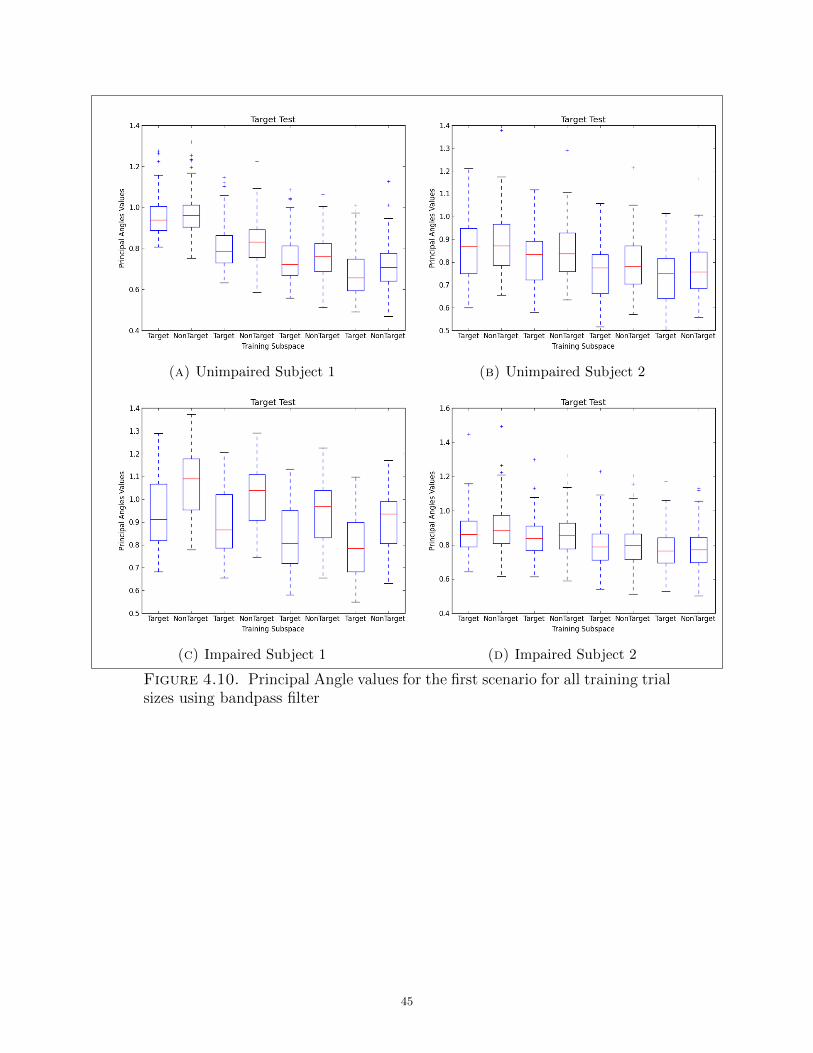
(a) Unimpaired Subject 1 (b) Unimpaired Subject 2
(c) Impaired Subject 1 (d) Impaired Subject 2
Figure 4.10. Principal Angle values for the first scenario for all training trialsizes using bandpass filter
45

(a) Unimpaired Subject 1 (b) Unimpaired Subject 2
(c) Impaired Subject 1 (d) Impaired Subject 2
Figure 4.11. Principal Angle values for the first scenario for all training trialsizes using bandpass filter
46

(a) Unimpaired Subject 1 (b) Unimpaired Subject 2
(c) Impaired Subject 1 (d) Impaired Subject 2
Figure 4.12. Principal Angle values for the second scenario for all trainingtrial sizes
47

(a) Unimpaired Subject 1 (b) Unimpaired Subject 2
(c) Impaired Subject 1 (d) Impaired Subject 2
Figure 4.13. Principal Angle values for the second scenario for all trainingtrial sizes
48

(a) Unimpaired Subject 1 (b) Unimpaired Subject 2
(c) Impaired Subject 1 (d) Impaired Subject 2
Figure 4.14. Principal Angle values for the second scenario for all trainingtrial sizes using bandpass filter
49

(a) Unimpaired Subject 1 (b) Unimpaired Subject 2
(c) Impaired Subject 1 (d) Impaired Subject 2
Figure 4.15. Principal Angle values for the second scenario for all trainingtrial sizes using bandpass filter
50
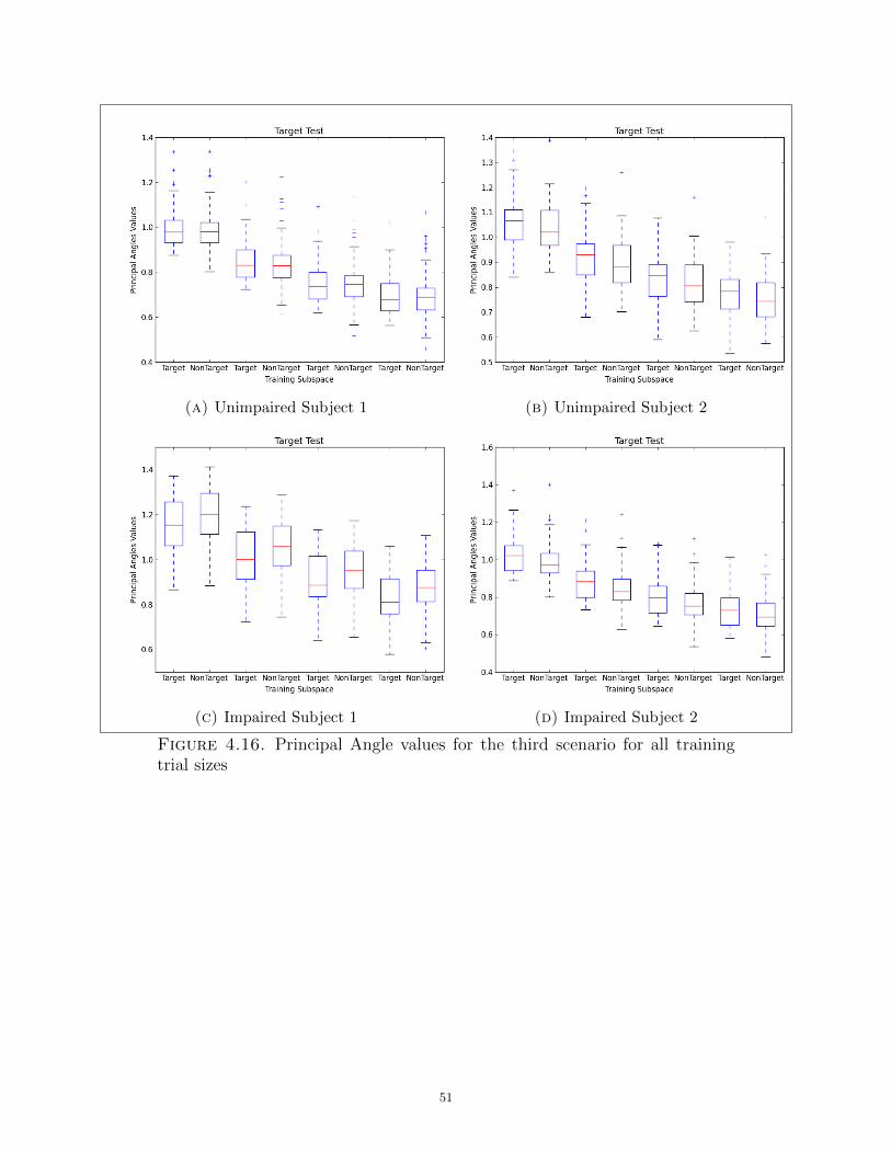
(a) Unimpaired Subject 1 (b) Unimpaired Subject 2
(c) Impaired Subject 1 (d) Impaired Subject 2
Figure 4.16. Principal Angle values for the third scenario for all trainingtrial sizes
51

(a) Unimpaired Subject 1 (b) Unimpaired Subject 2
(c) Impaired Subject 1 (d) Impaired Subject 2
Figure 4.17. Principal Angle values for the third scenario for all trainingtrial sizes
52

(a) Unimpaired Subject 1 (b) Unimpaired Subject 2
(c) Impaired Subject 1 (d) Impaired Subject 2
Figure 4.18. Principal Angle values for the third scenario for all trainingtrial sizes using bandpass filter
53

(a) Unimpaired Subject 1 (b) Unimpaired Subject 2
(c) Impaired Subject 1 (d) Impaired Subject 2
Figure 4.19. Principal Angle values for the third scenario for all trainingtrial sizes using bandpass filter
54

4.2. Outliers Removal Results
After the signals were smoothed, the classification process is implemented on both cases
with and without removing the outliers. In this section the results of removing the outliers
for all cases using either the minimum or the mean of the principal angles are shown. The
cases that are presented in this section are when the test subspace consists of 1 trial and the
training subspaces consist of 1, 2, 3, or 4 trials. All subjects were examined and the first
scenario of the impaired Subject 1’s outliers figures and numbers are demonstrated as an
example since the best P300 presentation is shown in this subject’s signals. In this scenario
as mentioned before, the combination of all letter trials is 60 for the target and 180 for the
nontarget. Data is divided into five different sets. Every time 48 trials are taken as target
training and the remaining 12 as a test. On the other hand, 144 trials are taken as nontarget
training and 36 as a testing trials. This process was implemented on all of the five disjoint
sets. Tables 4.3–4.6 show the number of the target and nontarget training subspaces after
removing the outliers from the training subspaces. Figures 4.20–4.25 show the training trials
before and after removing the outliers based on the minimum and the mean of the principal
angles. These figures illustrate the results of the first disjoint set as an example. In addition,
the training sizes that are shown as example are 1 and 2. As displayed in Figure 4.20 and
Figure 4.21, the number of the similarity measures is related to one principal angle only
since the size of the trial is one, while with Figures 4.22–4.25 the principal angles are 2 based
on the trial sizes as mentioned before. As shown in these figures, the value of the principal
angles using the minimum measurement tends to be less than the mean.
The Balanced accuracy is more stable and reliable compared with the accuracy that
was mentioned in the previous chapter. Figure 4.26 shows an example of the presented
experiments with 2 training trials and 1 testing trial. As mentioned before, the measure
55

Table 4.3. Number of Training Subspaces After Outlier Removal in the FirstScenario with training trial size is 1
Min PA1 Mean PA1Test No Target NonTarget Target NonTarget
Test 1 33 95 31 94Test 2 34 93 34 93Test 3 34 96 31 96Test 4 34 96 35 92Test 5 30 97 32 95
Table 4.4. Number of Training Subspaces After Outlier Removal in the FirstScenario with training trial size is 2
Min PA1 Min PA2 Mean PA1 Mean PA2Test No Target NonTarget Target NonTarget Target NonTarget Target NonTarget
Test 1 32 94 34 96 24 106 34 104Test 2 30 110 32 98 28 100 36 102Test 3 30 104 32 102 30 102 28 100Test 4 32 100 32 98 26 98 28 104Test 5 34 104 30 110 26 104 30 94
Table 4.5. Number of Training Subspaces After Outlier Removal in the FirstScenario with training trial size is 3. NT is the NonTarget.
Min PA1 Min PA2 Min PA3 Mean PA1 Mean PA2 Mean PA3TestNo
TargetNT TargetNT TargetNT TargetNT TargetNT TargetNT
Test 1 30 90 33 81 30 111 36 102 27 102 36 96Test 2 24 99 30 93 30 96 30 96 33 96 36 93Test 3 33 93 24 81 24 84 27 96 27 105 36 102Test 4 33 93 36 90 30 93 30 90 27 99 30 87Test 5 33 102 30 96 27 99 33 90 27 111 33 99
Table 4.6. Number of Training Subspaces After Outlier Removal in the FirstScenario with training trial size is 4. T is the Target and NT is the NonTarget.
Min PA1Min PA2Min PA3Min PA4Mean PA1Mean PA2Mean PA3Mean PA4TestNo
T NT T NT T NT T NT T NT T NT T NT T NT
Test 1 28 104 28 96 28 84 28 88 28 104 28 100 32 104 28 108Test 2 28 104 28 96 28 84 28 88 28 96 32 104 28 104 32 100Test 3 32 104 32 80 32 80 36 108 28 96 28 100 28 100 24 104Test 4 36 76 28 84 32 84 28 112 28 96 32 88 32 88 32 92Test 5 28 112 32 88 32 92 36 112 36 92 28 92 32 100 32 100
56
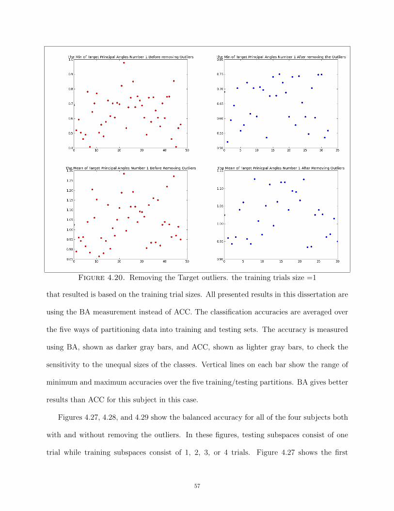
Figure 4.20. Removing the Target outliers. the training trials size =1
that resulted is based on the training trial sizes. All presented results in this dissertation are
using the BA measurement instead of ACC. The classification accuracies are averaged over
the five ways of partitioning data into training and testing sets. The accuracy is measured
using BA, shown as darker gray bars, and ACC, shown as lighter gray bars, to check the
sensitivity to the unequal sizes of the classes. Vertical lines on each bar show the range of
minimum and maximum accuracies over the five training/testing partitions. BA gives better
results than ACC for this subject in this case.
Figures 4.27, 4.28, and 4.29 show the balanced accuracy for all of the four subjects both
with and without removing the outliers. In these figures, testing subspaces consist of one
trial while training subspaces consist of 1, 2, 3, or 4 trials. Figure 4.27 shows the first
57

Figure 4.21. Removing the NonTarget outliers. the training trials size =1
scenario results, Figure 4.28 demonstrates the second scenario, and Figure 4.29 is for the
third scenario. As shown in these figures, in some cases no outlier removal tends to give
better results than removing the outliers. In some cases, removing the outliers increases
the accuracy a small percentage. Comparing Figures 4.27 with Tables 4.3–4.6 explain the
impaired Subject 1 training subspace sizes after removing the outliers in the first scenario.
In the case that the training size is 1, the outliers that were removed based on the minimum
of the first principal angle are less than the one that was removed based on the mean. Based
on this the BA tends to be higher with the minimum measurement than the mean. The same
results are reached in the case that the training size is 2. The minimum of the first principal
angle tends to increase the accuracy more than the mean of the first principal angle since
58

Figure 4.22. Removing the Target outliers based on the min and the meanof the first principal angle. the training trials size =2.
the number of the outliers that were removed is less with the minimum case. On the other
hand, with the second principal angles, both methods are similar to the outliers removing
number and BA results. In the case the training size is 3 and 4, the mean method tends to
be better than the minimum measurement in most cases because outliers are less removed.
We speculate that an outlier can have a large effect on trial averages that is commonly
used in BCI field, but an outlier as one of the trials used to define a subspace may have
much less effect on the principal angles between that subspace and other subspaces.
59

Figure 4.23. Removing the Target outliers based on the min and the meanof the second principal angle. the training trials size =2
60
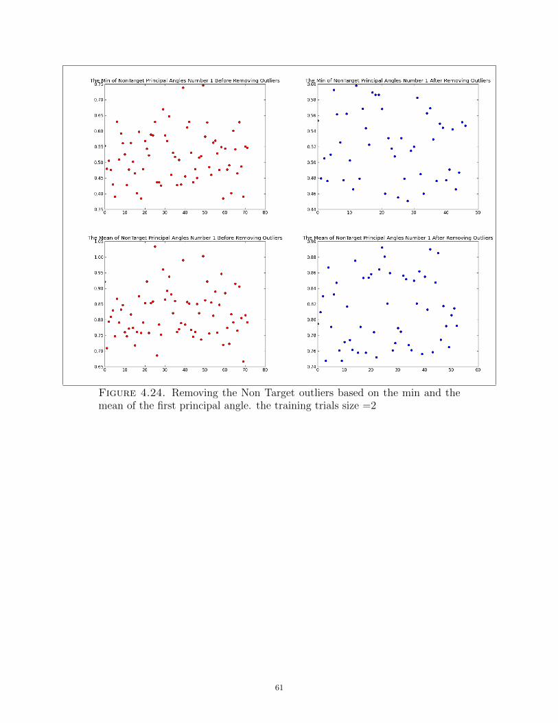
Figure 4.24. Removing the Non Target outliers based on the min and themean of the first principal angle. the training trials size =2
61

Figure 4.25. Removing the Non Target outliers based on the min and themean of the second principal angle. the training trials size =2
Figure 4.26. Classification accuracies as percentatge of test samples classi-fied correctly.
62

(a) Train size=1 (b) Train size=2
(c) Train size=3(d) Train size=4
Figure 4.27. The Balanced classification accuracy with and without remov-ing the outliers for the first scenario
(a) Train size=1 (b) Train size=2
(c) Train size=3(d) Train size=4
Figure 4.28. The Balanced classification accuracy with and without remov-ing the outliers for the second scenario
63
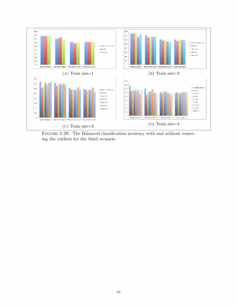
(a) Train size=1 (b) Train size=2
(c) Train size=3(d) Train size=4
Figure 4.29. The Balanced classification accuracy with and without remov-ing the outliers for the third scenario
64

4.3. The Evaluation of the Proposed Method Using different Trial Sizes
After presenting the preprocessing methods and the outlier removal results, this section
shows the results of changing not only the number of trials per training subspace, but also
per testing subspace. In this section, both testing and training sizes are either 1, 2, 3, or 4
trials and the combination between these options will be presented. The results are related
to the case that no outlier removal is used since, as shown in the previous section, outliers
rejection did not help that much and in some cases did not help at all. All of the three
scenarios are also demonstrated.
4.3.1. First Scenario. In this scenario, 60 trials are the target and 180 trials are
nontarget dividing to 48 target training trials and 12 target testing trials. On the other
hand, 144 nontarget training trials and 36 as a nontarget testing trials. The values of the
first principal angles between each testing subspace and training subspace are used. The
mean of these angles over all target training subspaces is compared with the mean of these
angles over all nontarget training subspaces. If the mean for the target subspaces is less than
the mean of the nontarget subspaces, the test subspace is calculated as a target subspace,
meaning one containing a P300. Otherwise, the testing subspace is classified as a nontarget.
An illustration of this comparison is shown in Figure 4.30. It plots the means of the
first principal angles between each of the 24 testing subspaces (6 target and 18 nontarget)
and all 96 (24 target and 72 nontarget) training subspaces in the case that training and
testing subspaces consist of 2 trials as an example. Each line corresponds to these means
for a single testing subspace. The endpoints of each line are the means of the first principal
angles between the testing subspace and the target and nontarget training subspaces. The
65
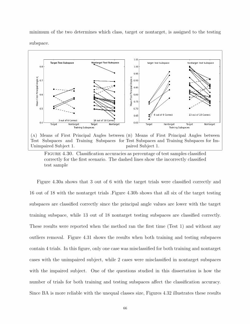
minimum of the two determines which class, target or nontarget, is assigned to the testing
subspace.
(a) Means of First Principal Angles betweenTest Subspaces and Training Subspaces forUnimpaired Subject 1.
(b) Means of First Principal Angles betweenTest Subspaces and Training Subspaces for Im-paired Subject 1.
Figure 4.30. Classification accuracies as percentage of test samples classifiedcorrectly for the first scenario. The dashed lines show the incorrectly classifiedtest sample
Figure 4.30a shows that 3 out of 6 with the target trials were classified correctly and
16 out of 18 with the nontarget trials .Figure 4.30b shows that all six of the target testing
subspaces are classified correctly since the principal angle values are lower with the target
training subspace, while 13 out of 18 nontarget testing subspaces are classified correctly.
These results were reported when the method ran the first time (Test 1) and without any
outliers removal. Figure 4.31 shows the results when both training and testing subspaces
contain 4 trials. In this figure, only one case was misclassified for both training and nontarget
cases with the unimpaired subject, while 2 cases were misclassified in nontarget subspaces
with the impaired subject. One of the questions studied in this dissertation is how the
number of trials for both training and testing subspaces affect the classification accuracy.
Since BA is more reliable with the unequal classes size, Figures 4.32 illustrates these results
66

(a) Means of First Principal Angles betweenTest Subspaces and Training Subspaces forUnimpaired Subject 1.
(b) Means of First Principal Angles betweenTest Subspaces and Training Subspaces for Im-paired Subject 1.
Figure 4.31. Classification accuracies as percentage of test samples classifiedcorrectly using 4 trials.The dashed lines show the incorrectly classified testsample
for all of the four subjects using all the different combinations of the trial sizes. As shown
(a) Unimpaired Subject 1 (b) Unimpaired Subject 2
(c) Impaired Subject 1 (d) Impaired Subject 2
Figure 4.32. Classification balanced accuracies average for all trial sizes inthe first scenario.
67

in Figures 4.32 for most cases when training subspaces created using 2 trials and testing
subspaces formed using four trials, the BA values tends to be better than other cases. On
the other hand for the impaired Subject 2, the best BA was reached using 1 trial only for the
training subspaces and 3 trials for testing subspaces. The best accuracy was 90% for both
the unimpaired Subject 1 and the impaired Subject 1, 74% for the unimpaired Subject 2,
and 77% for the impaired Subject 2. Comparing between subjects, the impaired Subject 1
tends to give the best results and the impaired Subject 2 tends to give the lowest BA in
most cases.
4.3.2. Second Scenario. In this scenario, the method is tested on each subject using
both letters p and b as a train data and letter d as a test data. The idea from this scenario is
testing the method on different data than the training dataset, which means more variations
between the training and testing data since the training data subspaces do not include any
of the letter-d information.
The steps in this scenario are similar to the previous one. First, the training data is
smoothed. The training subspaces dimensionalities are 40 target trials and 120 nontarget,
while for the testing subspaces they are 20 for the target and 60 for the nontarget. Since
five testing times are applied, different testing trials are examined in each step. According
to this in each testing time, 4 target and 12 nontarget disjoint trials are selected. Results
demonstrate in Figures 4.33 is the caes that training and testing subspaces are created using
2 trials only.
Figure 4.33a shows that all of the nontarget trials, which are related to the unimpaired
subject are classified correctly and only one target trial was misclassified. Figure 4.33b is
the results that are related to the impaired subject. All target trials are identified correctly,
while only one of the nontarget trials is misclassified. These results were reached by using
68

(a) Means of First Principal Angles betweenTest Subspaces and Training Subspaces forUnimpaired Subject 1.
(b) Means of First Principal Angles betweenTest Subspaces and Training Subspaces for Im-paired Subject 1.
Figure 4.33. Classification accuracies as percentage of test samples classi-fied correctly for the second scenario.The dashed lines show the incorrectlyclassified test sample
the first 4 trials from the testing target trials and first 12 trials from the testing nontarget.
These results are before removing any of the principal angles outliers.
Figure 4.34 demonstrates that in most cases defining the training and testing subspaces
with 4 trials tends to give better results than other cases except for the unimpaired Subject 2
gives better results when having 3 trials in the testing subspaces only and 4 trials with the
training subspaces. Similar to the first scenario, the impaired Subject 1 tends to give the
best results, while the impaired Subject 2 tends to be the lowest results in most cases. The
highest BA for the unimpaired Subject 1 is 83%, for the unimapred Subject 2 is 85%. In
addition, with impaired cases the BA for Subject 1 is 97% and it is 77% for Subject 2.
4.3.3. Third Scenario. In this section, the presented method is trained on three sub-
jects and tested on the fourth subject. In this case, the training target trial number is 180
and 540 for the nontarget. Testing trials are 60 and 180 for target and nontarget, but because
five different testing subspaces will be examined, each time 12 target trials and 36 for the
69

(a) Unimpaired Subject 1 (b) Unimpaired Subject 2
(c) Impaired Subject 1 (d) Impaired Subject 2
Figure 4.34. Classification accuracies average for all trial sizes in the secondscenario.
nontarget will be evaluated. As a start point, two subjects were tested such as unimapired
Subject 1 and imapired Subject 1 with pairs trials only before evaluating the method on all
subjects with all trial sizes. As shown in Figure 4.35 the method classified correctly all target
trials if training was on the unimapired Subject 1, while there were four misclassification
if training was on the imapired Subject 1. In addition, for nontarget trials all trials were
classified correctly if the training was on the imapired Subject 1, while only 8 cases were
classified correctly if the training was on the unimapired Subject 1.
Figure 4.36 demonstrates the BA for testing on all four users separately using the infor-
mation from other three users. In this figure, it is shown that with unimpaired cases testing
subspaces with 4 trials tends to give better results, while having 1 trial only to create the
training subspaces tends to be better. Tesing on the impaired Subject 1 tends to give the
highest BA and tesing on the second impaired subject tends to give the lowest BA. The best
classification result when testing on unimpaired Subject 1 is 82% and 69% when testing on
70
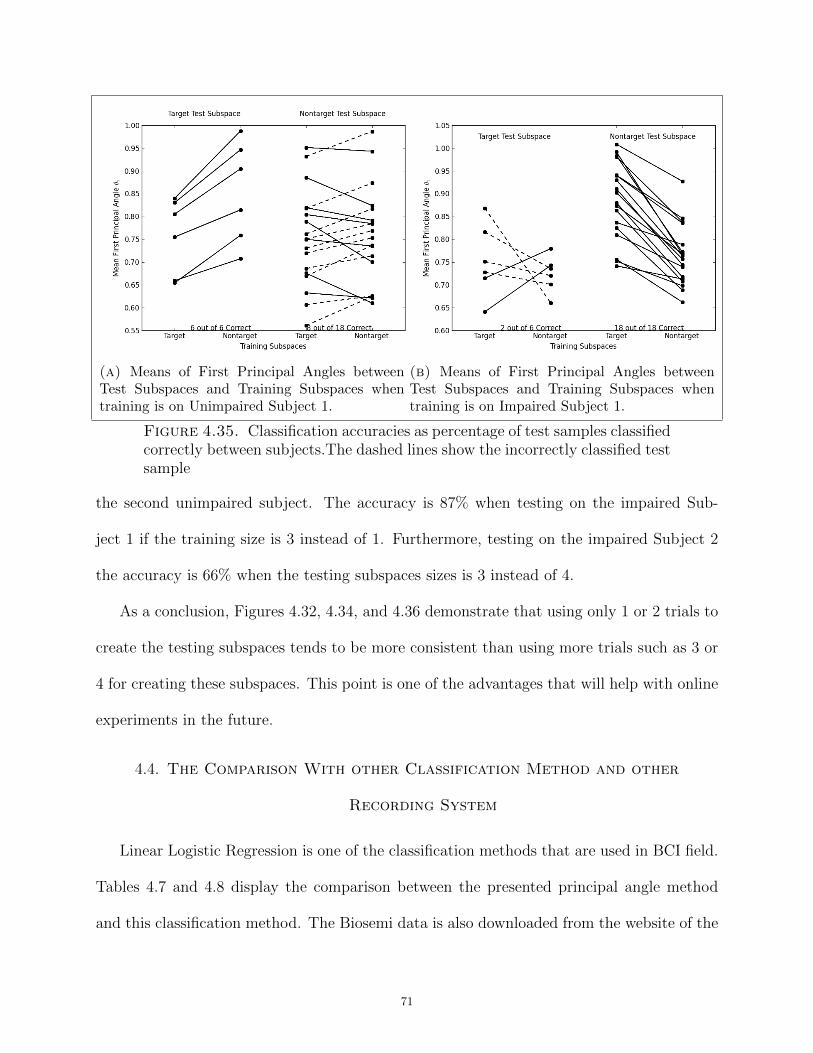
(a) Means of First Principal Angles betweenTest Subspaces and Training Subspaces whentraining is on Unimpaired Subject 1.
(b) Means of First Principal Angles betweenTest Subspaces and Training Subspaces whentraining is on Impaired Subject 1.
Figure 4.35. Classification accuracies as percentage of test samples classifiedcorrectly between subjects.The dashed lines show the incorrectly classified testsample
the second unimpaired subject. The accuracy is 87% when testing on the impaired Sub-
ject 1 if the training size is 3 instead of 1. Furthermore, testing on the impaired Subject 2
the accuracy is 66% when the testing subspaces sizes is 3 instead of 4.
As a conclusion, Figures 4.32, 4.34, and 4.36 demonstrate that using only 1 or 2 trials to
create the testing subspaces tends to be more consistent than using more trials such as 3 or
4 for creating these subspaces. This point is one of the advantages that will help with online
experiments in the future.
4.4. The Comparison With other Classification Method and other
Recording System
Linear Logistic Regression is one of the classification methods that are used in BCI field.
Tables 4.7 and 4.8 display the comparison between the presented principal angle method
and this classification method. The Biosemi data is also downloaded from the website of the
71

(a) Tested on Unimpaired Subject 1 (b) Tested on Unimpaired Subject 2
(c) Tested on Impaired Subject 1 (d) Tested on Impaired Subject 2
Figure 4.36. Classification accuracies average for all trial sizes in the thirdscenario.
CSU BCI research group. The Biosemi system is used to record thirty two- channels EEG
with a 1024 Hz sampling rate. The channel that was used in this comparison is also P4. Four
more subjects were added for the G.tec recording system, two as unimpaired subjects and
two as impaired. For both G.tec and Biosemi, the presented smoothing method is applied
before classifying the signals using either the Linear Logistic Regression or the subspaces
and the principal angles. The results are related to the experiment that is similar to the
second scenario. In this case, the training was on letter-b and letter-d, while the testing
was on letter-p. This experiment was chosen to match the scenario that was followed by
the CSU BCI research group on their tests to reach their results. The results were obtained
by creating the testing subspaces using one trial only. Figures 4.37 - 4.40 display the EEG
signals that are recorded using the Biosemi system before and after smoothing preprocessing
step.
72

Comparing between classification methods, Tables 4.7 shows that the proposed principal
angle (PA) method tends to classify the testing trials that are related to the unimpaired sub-
jects more accurately than the Linear Logistic Regression method, except for the unimpaired
Subject 4. On the other hand, the Linear Logistic Regression method tends to give higher
classification accuracy than the principal angle method for the impaired subjects, except
with impaired Subject 3. Similar to the previous results, both classification methods give
the highest BCA with the impaired Subject 1 and unimpaired Subject 2 since their EEG
signal seems to display P300 representation clearer than the other two subjects. Table 4.8
shows that with the Biosemi data, the BCA results vary between the classification methods.
In some cases the presented PA method tends to be better, but for other cases the Linear
Logistic Regression tends to give better BCA. Dividing the data into subspaces with single
or four trials only tends to give a big improvement with the impaired Subject 2 comparing
with the other classification method that considered the whole training data. computation
time was measured on Apple MacBook Pro with 2.7 GHz Intel Core i7.
Comparing between the two recording systems, the G.tec system needs less time to
classify a testing trial to either target or nontarget than Biosemi system since the sampling
rate with G.tec is less than Biosemi. For example, to classify a single trial that is related to
unimpaired Subject 1, 8 seconds are needed using 2 trials for creating the training subspaces.
On the other hand, 28 seconds are needed to classify a single Bioesemi trial for the same
subject using also only 2 trials for developing the training subspaces.
Tables 4.7 and 4.8 demonstrate that as an average the PA method tends to give better
BCA results than the Linear Logistic Regression method using either G.tec or Biosemi
recording systems. Comparing between the recording systems with different sampling rates,
73

Table 4.7. Comparison between the classification accuracies g.tec g.MOBILab+
Subject No. Linear Logistic Regression PABCA (Training) BCA (Testing) λ BCA λ Train Trial Size
Unimpaired Subject 1 78.8 63.3 0.0001 71.7 0.0001 2Unimpaired Subject 2 78.3 51.7 0.0001 60.8 0.0001 1Unimpaired Subject 3 80.0 52.5 0.0001 60.0 0.0001 4Unimpaired Subject 4 73.3 56.7 0.0001 54.2 0.0001 3Impaired Subject 1 94.2 75.8 0.0001 71.7 0.0001 3Impaired Subject 2 76.7 55.0 0.0001 54.2 0.0001 4Impaired Subject 3 80.0 55.1 0.0001 62.5 0.0001 2Impaired Subject 4 72.1 55.0 0.0001 51.7 0.0001 1Average 58.1 60.9
both classification methods in most cases tend to give lower BCA using Biosemi recording
system with a higher sampling rate.
This section shows that for some cases the proposed PA method tends to give better
results than the Linear Logistic Regression method, but not for all cases. The following
are possible explanations. First, the Linear Logistic Regression is trained on all training
data, while PA method divides the training data into multiple subspaces. This concept
helps to increase the BCA when the data is very noisy such as the cases of the impaired
Subject 2 with G.tec system and unimpaired Subject 2 with Biosemi system as shown in
both Table 4.7 and Table 4.8. The second reason is when the data is not very noisy, dividing
the training data into small subspaces with training trial sizes one, three, or four helps to
increase the BCA results. This thought is clearly presented with unimpaired Subject 1 and 2
using G.tec system and with unimpaired Subject 1 and impaired Subject 2 using Biosemi
data. Figure 4.39 and Figure 4.40 display that dividing the training subspaces into small
sets, calculating the principal angles between testing trials and these sets, and finding the
matching set based on the smallest angles improves the BCA specially with the time between
500 ms and 600 ms.
74

Table 4.8. Comparison between the classification accuracies Biosemi ActiveTwo
Subject No. Linear Logistic Regression PABCA (Training) BCA (Testing) λ BCA λ Train Trial Size
Unimpaired Subject 1 81.8 57.5 0.0001 60.8 0.0001 2Unimpaired Subject 2 80.0 63.3 0.0001 60.8 0.0001 4Impaired Subject 1 98.8 74.2 0.0001 63.3 0.0001 3Impaired Subject 2 75.4 47.5 0.0001 65.0 0.0001 1,4Average 60.6 62.5
(a) Unimpaired Subject 1 (b) Unimpaired Subject 2
(c) Impaired Subject 1 (d) Impaired Subject 2
Figure 4.37. Biosemi Target Signals for all 4 Subjects before smoothing step
75
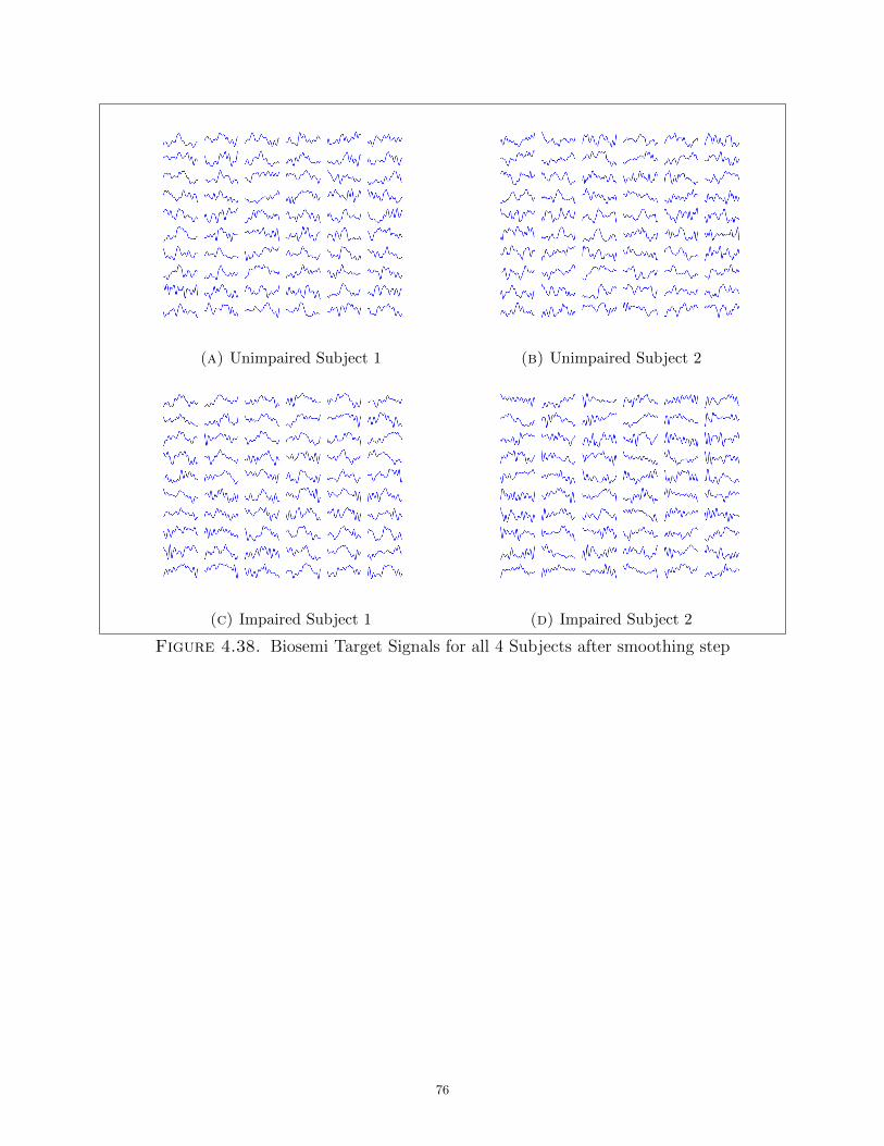
(a) Unimpaired Subject 1 (b) Unimpaired Subject 2
(c) Impaired Subject 1 (d) Impaired Subject 2
Figure 4.38. Biosemi Target Signals for all 4 Subjects after smoothing step
76
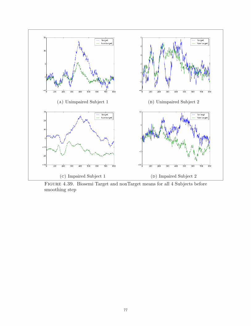
(a) Unimpaired Subject 1 (b) Unimpaired Subject 2
(c) Impaired Subject 1 (d) Impaired Subject 2
Figure 4.39. Biosemi Target and nonTarget means for all 4 Subjects beforesmoothing step
77

(a) Unimpaired Subject 1 (b) Unimpaired Subject 2
(c) Impaired Subject 1 (d) Impaired Subject 2
Figure 4.40. Biosemi Target and nonTarget means for all 4 Subjects aftersmoothing step
78

CHAPTER 5
Conclusion and Future Work
EEG was recorded from four subjects, two with motor impairment and two with no
impairments. EEG data following presentations of single letters in the center of a computer
display was collected while the subjects counted the occurrences of particular letters, in order
to produce P300 waves. Three different experiments and scenarios were evaluated such as
combine all of the three target letters and exclude some of the trials from this combination
to be considered as a testing subspaces. In addition, creating the training subspaces using
the data of two target letters and left one target letter as a testing subspaces to evaluate
the classifier on more variations between the training and testing subspaces. Furthermore,
examining the transfer information between subjects by creating the training subspaces using
the data that are recorded from three different subjects and testing the method on the fourth
subject.
Before the subspaces are created, a smoothing function is applied to filter the signals from
the noise. Two different methods were tested, smoothing by regularization and bandpass
filter. Typically bandpass filters are applied, but the smoothing algorithm demonstrated
here does not rely on assumptions on the frequency content of EEG as required for bandpass
filtering. No clear trends were found between these two methods. This study also examines
ways of removing outliers that are based on principal angles. While the experiments show
that the outlier removal methods did not help in this case, they may prove useful for other
subjects or signals. This means that having an outlier as one of the trials that is used to
create the subspace could not effect that much on the principal angles between this subspace
and the other subspaces unlike other methods that depend on the trial averages concept.
79

In the first scenario, balanced classification accuracies of 90% and 74% were obtained for
the unimpaired and 90% and 77% for the impaired subjects respectively, using one or two
trials per subspace. In the second scenario, the accuracy was 83% and 85% for unimpaired
subjects and 97% and 77% for impaired subjects using four trials per subspace. In the third
scenario, having one or three training trials gives 82% and 69% as a balanced accuracy if
the testing was on the unimpaired subjects and 87% and 66% accuracy if the testing was on
the impaired subject. This accuracy is similar to other published studies on P300 detection.
However, most other approaches use averages of more trials to obtain similar accuracies.
The use of only a small number of trials makes this approach more appropriate for online
application. Comparing the proposed method with the Linear Logistic Regression, principal
angles method tends to give better results than the other method as an average of the
all subjects. PA tends to produce results that are about 3% better than Linear Logistic
Regression for the G.tec system and 2% using the Biosemi system.
Analyzing EEG patterns using principal angles is still a new direction in BCI field.
Many studies can be implemented and added to this field to better analyze and classify
the EEG patterns. Planned future work in this study includes the use of additional data
sets recorded from other subjects, other recording systems with different sampling rates. As
mentioned before in Chapter 2, the best accuracies in published results from the studies
with the Competition data, some which are reviewed in this Chapter, are 40%-60% using
single trial. The accuracies obtained in this dissertation are about 60%-80% for single trial.
This warrants additional testing of the methods that were developed in this dissertation on
the BCI Competition data [29]. Plans also include analyzing using additional channels and
the use of other principal angle methods that are previously described in Chapter 2, such
as the Discriminant Canonical Correlation (DCC) [23] method, that discriminates between
80

subspaces by maximizing the canonical correlation within the subspace and minimizing it
between the subspaces. In addition, applying EEG subspace analysis using the principal
angles concept with online and mental tasks experiments and using the principal angles
to find the best template in training subspaces that present the P300 clearly. Creating
the subspaces by shifting in time, which means each trial contains information from the
previous trial, might help to have more information in the trial and make the principal
angle values correct to give better classification. Since most of the concentration in this
dissertation is on the principal angles and analyzing the values of theses angles, studying
and evaluating the principal vectors that are connected to these angles is a good direction
to learn more deeply about how these vectors look like with the target P300 cases and non
P300 trials. Furthermore, the similarities and differences of the vector variations within and
across subspaces should be studied.
81

Bibliography
[1] J. R. Wolpaw, N. Birbaumer, D. J. McFarland, G. Pfurtscheller, and T. M. Vaughan,
“Brain–computer interfaces for communication and control,” Clinical neurophysiology,
vol. 113, no. 6, pp. 767–791, 2002.
[2] M. Khazi, A. Kumar, and M. Vidya, “Analysis of eeg using 10: 20 electrode system,”
International Journal of Innovative Research in Science, Engineering and Technology,
vol. 1, no. 2, pp. 185–191, 2012.
[3] T. Al-ani and D. Trad, Signal Processing and Classification Approaches for Brain-
computer Interface. INTECH Open Access Publisher, 2010.
[4] G. Strang, Introduction to Linear Algebra 4e. Wellesley-Cambridge Press, 2009.
[5] J. Chang, Classification on the Grassmannians: Theory and Applications. PhD thesis,
Colorado State University, 2008.
[6] M. Thulasidas, C. Guan, and J. Wu, “Robust classification of eeg signal for brain-
computer interface,” Neural Systems and Rehabilitation Engineering, IEEE Transac-
tions on, vol. 14, no. 1, pp. 24–29, 2006.
[7] A. Turnip and K.-S. Hong, “Classifying mental activities from eeg-p300 signals using
adaptive neural networks,” Int. J. Innov. Comput. Info. Control, vol. 8, no. 9, pp. 6429–
6443, 2012.
[8] J. Elshout and G. G. Molina, “Review of brain-computer interfaces based on the p300
evoked potential,” tech. rep., Koninklijke Philips Electronics, 2009.
[9] M. T. Harandi, C. Sanderson, S. Shirazi, and B. C. Lovell, “Graph embedding discrim-
inant analysis on grassmannian manifolds for improved image set matching,” in Com-
puter Vision and Pattern Recognition (CVPR), 2011 IEEE Conference on, pp. 2705–
2712, IEEE, 2011.
82

[10] R. Wang, S. Shan, X. Chen, and W. Gao, “Manifold-manifold distance with application
to face recognition based on image set,” in Computer Vision and Pattern Recognition,
2008. CVPR 2008. IEEE Conference on, pp. 1–8, IEEE, 2008.
[11] J. J. Stickel, “Data smoothing and numerical differentiation by a regularization method,”
Computers & Chemical Engineering, vol. 34, no. 4, pp. 467–475, 2010.
[12] X. ou Li, F. Wang, X. Chen, and R. Ward, “A p300-based bci classification algorithm
using median filtering and bayesian feature extraction,” in Multimedia Signal Processing
(MMSP), 2012 IEEE 14th International Workshop on, pp. 305–308, Sept 2012.
[13] F. Lotte, M. Congedo, A. Lecuyer, F. Lamarche, B. Arnaldi, et al., “A review of clas-
sification algorithms for eeg-based brain–computer interfaces,” Journal of Neural Engi-
neering, vol. 4, pp. R1–R13, 2007.
[14] P. Van Overschee and B. De Moor, Subspace Identification for Linear Systems: Theory
- Implementation - Applications. Springer London, Limited, 2011.
[15] P. Zhu and A. V. Knyazev, “Angles between subspaces and their tangents,” Apr. 2013.
arXiv:1209.0523[math.NA].
[16] M. E. Argentati, Principal angles between subspaces as related to Rayleigh quotient and
Rayleigh Ritz inequalities with applications to eigenvalue accuracy and an eigenvalue
solver. PhD thesis, University of Colorado, 2003.
[17] A. V. Knyazev and M. E. Argentati, “Principal angles between subspaces in an a-based
scalar product: Algorithms and perturbation estimates,” SIAM J. SCI. COMPUT,
vol. 23, no. 6, pp. 2009–2041, 2002.
[18] C. Shan, “Face recognition and retrieval in video,” in Video Search and Mining, pp. 235–
260, Springer, 2010.
83

[19] T.-K. Kim, O. Arandjelovic, and R. Cipolla, “Boosted manifold principal angles for
image set-based recognition,” Pattern Recognition, vol. 40, no. 9, pp. 2475–2484, 2007.
[20] O. Arandjelovic and R. Cipolla, “Face recognition from face motion manifolds using
robust kernel resistor-average distance,” in Computer Vision and Pattern Recognition
Workshop, 2004. CVPRW’04. Conference on, p. 88, IEEE, 2004.
[21] T.-K. Kim, O. Arandjelovic, and R. Cipolla, “Learning over sets using boosted manifold
principal angles (bompa),” in In Proc. British Machine Vision Conference,, pp. 779–788,
2005.
[22] Y. M. Lui, J. Beveridge, B. Draper, and M. Kirby, “Image-set matching using a geodesic
distance and cohort normalization,” in Automatic Face Gesture Recognition, 2008. FG
’08. 8th IEEE International Conference on, pp. 1–6, Sept 2008.
[23] T.-K. Kim, J. Kittler, and R. Cipolla, “Discriminative learning and recognition of image
set classes using canonical correlations,” Pattern Analysis and Machine Intelligence,
IEEE Transactions on, vol. 29, no. 6, pp. 1005–1018, 2007.
[24] Y. Freund and R. E. Schapire, “A short introduction to boosting,” in In Proceedings of
the Sixteenth International Joint Conference on Artificial Intelligence, pp. 1401–1406,
Morgan Kaufmann, 1999.
[25] P. Melville, N. Shah, L. Mihalkova, and R. J. Mooney, “Experiments on ensembles with
missing and noisy data,” in Multiple Classifier Systems, pp. 293–302, Springer, 2004.
[26] J. mei Chang and J. I. Pacheco, “Classifying handwritten digits on the grassmann man-
ifold,” in Proceedings of the International Conference on Image Processing Computer
Vision, and Pattern Recognition, vol. 1, pp. 36–41, 2011.
84

[27] C. Anderson and M. Kirby, “Eeg subspace representations and feature selection for
brain-computer interfaces,” in Computer Vision and Pattern Recognition Workshop,
2003. CVPRW ’03. Conference on, vol. 5, p. 51, June 2003.
[28] W. Samek, F. Meinecke, and K. Muller, “Transferring subspaces between subjects in
brain computer interfacing,” in IEEE Transactions on Biomedical Engineering, vol. 60,
pp. 2289–2298, August 2013.
[29] “Bci competition III.” http://www.bbci.de/competition/iii/.
[30] H. Liu, X. Wang, and L. Gan, “Electroencephalograph automatic diagnosis based on
kernel principal angle,” in Advances in Electronic Commerce, Web Application and
Communication, pp. 487–492, Springer, 2012.
[31] Y. M. Lui, J. R. Beveridge, B. A. Draper, and M. Kirby, “Image-set matching using a
geodesic distance and cohort normalization,” in Automatic Face & Gesture Recognition,
2008. FG’08. 8th IEEE International Conference on, pp. 1–6, IEEE, 2008.
[32] J. Chuang, H. Nguyen, C. Wang, and B. Johnson, “I think, therefore i am: Usability
and security of authentication using brainwaves,” in Financial Cryptography and Data
Security, pp. 1–16, Springer, 2013.
[33] N. V. Manyakov, N. Chumerin, A. Combaz, and M. M. Van Hulle, “Comparison of
classification methods for p300 brain-computer interface on disabled subjects,” Intell.
Neuroscience, vol. 2011, pp. 2:1–2:12, Jan. 2011.
[34] A. Bakhshi and A. Ahmadifard, “A comparison among classification accuracy of neural
network, flda and blda in p300-based bci system,” International Journal of Computer
Applications, vol. 46, pp. 11–15, May 2012.
85

[35] S. Hutagalung, A. Turnip, and A. Munandar, “P300 detection based on extraction and
classification in online bci,” in Instrumentation Control and Automation (ICA), 2013
3rd International Conference on, pp. 35–38, Aug 2013.
[36] F. Farooq and P. Kidmose, “Random forest classification for p300 based brain computer
interface applications,” in Signal Processing Conference (EUSIPCO), 2013 Proceedings
of the 21st European, pp. 1–5, Sept 2013.
[37] J. R. Wolpaw and D. J. McFarland, “Control of a twodimensional movement signal by
a non-invasive braincomputer interface in humans, published by,” in Proceedings of the
National Academy of Sciences of the United States of America, p. 51.
[38] “CEBL: CSU EEG and BCI lab software.” http://www.cs.colostate.edu/eeg, 2014.
[39] R. Ashari and C. Anderson, “EEG subspace Analysis and Classification Using Principal
Angles for Brain Computer Interfaces ,” in IEEE Symposium Series on Computational
Intelligence, pp. 57–63, Dec 2014. doi :10.1109/CIBCI.2014.7007793.
[40] S. Straube and M. M. Krell, “How to evaluate an agent’s behavior to infrequent event?
– reliable performance estimation insensitive to class distribution,” Frontiers in Com-
putational Neuroscience, vol. 8, no. 43, 2014. doi :10.3389/fncom.2014.00043.
86