DISSERTATION

DEVELOPMENT OF A HIERARCHICAL ELECTROSPUN SCAFFOLD FOR LIGAMENT

REPLACEMENT

Submitted by

Hannah Marie Pauly

Graduate Degree Program in Bioengineering

In partial fulfillment of the requirements

For the Degree of Doctor of Philosophy

Colorado State University

Fort Collins, Colorado

Spring 2018

Doctoral Committee: Advisor: Tammy L. Haut Donahue

Jeremiah Easley Daniel J. Kelly Ross Palmer

Ketul C. Popat

Copyright by Hannah Marie Pauly 2018

All Rights Reserved

ii

ABSTRACT

DEVELOPMENT OF A HIERARCHICAL ELECTROSPUN SCAFFOLD FOR LIGAMENT

REPLACEMENT

The anterior cruciate ligament (ACL) is a dense collagenous structure that connects the femur to

the tibia and is vital for joint stability. The ACL possesses complex time-dependent viscoelastic

properties and functions primarily to prevent excessive translations and rotations of the tibia

relative to the femur. It is estimated that 400,000 ACL tears occur in the United States annually

and the monetary burden of these injuries and their subsequent treatment is approximately $1

billion annually. After injury allografts and autografts are commonly implanted to reconstruct the

torn ACL in an attempt to restore joint stability, prevent pain, and limit damage to surrounding

tissues. However surgical reconstructions fail to completely restore knee functionality or prevent

additional injury and regardless of intervention technique radiographic osteoarthritis is present in

13% of patients 10 years after ACL rupture.

Drawbacks to traditional treatments for ACL ruptures motivate the development of a synthetic

ACL replacement. Tissue engineering is the use of a scaffold, cells, and signaling molecules to

create a replacement for damaged tissue. The goal of this work is to develop a polymer scaffold

that can be utilized as a replacement for the ACL. A tissue engineered ACL replacement should

replicate the hierarchical structure of the native ACL, possess reasonable time zero mechanical

properties, and promote the deposition of de novo collagenous tissue in vitro. Additionally, the

iii

scaffold should be implantable using standard surgical techniques and should maintain in situ

tibiofemoral contact mechanics. Thus, four specific aims are proposed:

1) Fabricate and characterize an aligned 3-dimensional electrospun scaffold for ACL

replacement.

2) Assess the in vitro behavior of ovine bone marrow-derived stems cells seeded on the

scaffold in the presence of conjugated growth factor.

3) Evaluate the performance of the electrospun scaffold using uniaxial mechanical testing.

4) Assess the effect of the electrospun scaffold on ovine stifle joint contact mechanics.

Development of a tissue engineered ACL replacement that mimics the structure and function of

the native ACL would provide a novel treatment to improve outcomes of ACL injuries.

iv

ACKNOWLEDGEMENTS

First and foremost I must acknowledge the outstanding mentorship given to me by my advisor Dr.

Tammy Haut Donahue. I have benefited so much from your leadership, expertise, and advice. I will

forever be grateful for all your help throughout my time in the lab, both professionally and personally.

You have been an outstanding advisor every step of the way.

I would also like to thank my committee members Dr. Daniel Kelly, Dr. Ketul Popat, Dr. Ross Palmer,

and Dr. Jeremiah Easley, for their insightful feedback and commitment to this project. Special recognition

goes to our collaborators at Trinity College Dublin and Queens University, Belfast, Dr. Nicholas Dunne,

Dr. Shreekanth Pentlavalli, Dr. Philip Chambers, Dr. Binulal Sathy, and Dinorath Olvera for helping to

foster an outstanding international collaboration.

Without my lab mates, particularly Adam Abraham, Ben Wheatley, Kristine Fischenich, Brett Steineman,

and Gerardo Narez, this work would not have been possible or nearly as fun. Thank you for constantly

being there to assist, commiserate, and celebrate all things both in and out of the lab. Special thanks also

go to friends and collaborators who have helped along the way: Nicole Ramo, Laura Place, Nathan

Trujillo, Nabila Huq, Michael Gallen, and all my family and friends both near and far.

And finally to my fiancé Zach, thank you for your constant love and encouragement. I am so thankful that

I get to tackle every day with you by my side.

This work was supported by the National Science Foundation under Grant No. DMR 1306741 and

through the US-Ireland R&D Partnership Programme (USI 004. SRI-12/US/I2489).

v

DEDICATION

To my parents, Jim and Carol, and my brother, Nathan. I could not have been so happy, secure,

and successful so far from home without knowing that I had your unwavering love and support.

vi

TABLE OF CONTENTS

ABSTRACT .............................................................................................................................. ii ACKNOWLEDGEMENTS........................................................................................................ iv DEDICATION ............................................................................................................................ v LIST OF TABLES ..................................................................................................................... ix LIST OF FIGURES .................................................................................................................... x

CHAPTER 1: INTRODUCTION ................................................................................................ 1 1.1 ACL ANATOMY AND STRUCTURE ..................................................................... 1 1.1.1 ANATOMY AND PHYSIOLOGY ............................................................. 2 1.1.2 COMPOSITION AND HIERARCHICAL STRUCTURE ........................... 4 1.1.3 MECHANICAL FUNCTION AND MATERIAL PROPERTIES ............... 6 1.2 ACL INJURIES AND TREATMENTS .................................................................... 9 1.2.1 EPIDEMIOLOGY ....................................................................................... 9 1.2.2 TREATMENTS AND OUTCOMES ......................................................... 11 1.3 ACL TISSUE ENGINEERING ............................................................................... 13 1.3.1 SCAFFOLDS ............................................................................................ 14 1.3.2 CELLS AND SIGNALING MOLECULES ............................................... 17 1.4 OVINE STIFLE MODEL ........................................................................................ 20 1.5 SPECIFIC AIMS ..................................................................................................... 23 REFERENCES ......................................................................................................................... 26 CHAPTER 2: MECHANICAL PROPERTIES AND CELLULAR RESPONSE OF NOVEL ELECTROSPUN NANOFIBERS FOR LIGAMENT TISSUE ENGINEERING: EFFECTS OF ORIENTATION AND GEOMETRY ........................................................................................ 36 2.1 INTRODUCTION ................................................................................................... 36

2.2 EXPERIMENTAL MATERIALS AND METHODS ............................................... 39 2.2.1 FABRICATION OF NANOFIBER SHEETS AND BUNDLES ................ 39 2.2.2 CHARACTERIZATION OF NANOFIBER SHEETS AND BUNDLES ... 41 2.2.3 MECHANICAL TESTING ....................................................................... 43 2.2.4 CELL CULTURE ..................................................................................... 46 2.2.5 STATISTICS ............................................................................................ 48 2.3 RESULTS ............................................................................................................... 48

2.3.1 FABRICATION AND CHARACTERIZATION OF NANOFIBER SHEETS AND BUNDLES ................................................................................ 48

2.3.2 MECHANICAL TESTING ....................................................................... 49 2.3.3 CELL CULTURE ..................................................................................... 50 2.4 DISCUSSION.......................................................................................................... 54 2.5 CONCLUSIONS ..................................................................................................... 57 REFERENCES ......................................................................................................................... 64

vii

CHAPTER 3: HIERARCHICALLY STRUCTURED ELECTROSPUN SCAFFOLDS WITH CHEMICALLY CONJUGATED GROWTH FACTOR FOR LIGAMENT TISSUE ENGINEERING ....................................................................................................................... 70 3.1 INTRODUCTION ................................................................................................... 70 3.2 METHODS.............................................................................................................. 73

3.2.1 SCAFFOLD FABRICATION ................................................................... 73 3.2.2 GROWTH FACTOR CONJUGATION ..................................................... 74 3.2.3 HARVEST OF BONE MARROW-DERIVED STEM CELLS .................. 77 3.2.4 SHORT-TERM IN VITRO CELL CULTURE ........................................... 78

3.2.5 LONG-TERM IN VIVO CELL CULTURE ............................................... 79 3.2.6 IN VIVO SUBCUTANEOUS IMPLANTATION ...................................... 81 3.2.7 STATISTICS ............................................................................................ 82 3.3 RESULTS ............................................................................................................... 82

3.3.1 GROWTH FACTOR CONJUGATION ..................................................... 82 3.3.2 SHORT-TERM IN VITRO CELL CULTURE ........................................... 83 3.3.3 LONG-TERM IN VIVO CELL CULTURE ............................................... 85 3.3.4 IN VIVO SUBCUTANEOUS IMPLANTATION ...................................... 88

3.4 DISCUSSION.......................................................................................................... 90 REFERENCES ......................................................................................................................... 99 CHAPTER 4: MECHANICAL PROPERTIES OF A HIERARCHICAL ELECTROSPUN SCAFFOLD FOR OVINE ANTERIOR CRUCIATE LIGAMENT REPLACEMENT ............ 105 4.1 INTRODUCTION ................................................................................................. 105 4.2 METHODS............................................................................................................ 107 4.2.1 ELECTROSPUN SCAFFOLD FABRICATION ..................................... 107 4.2.2 SURGICAL TECHNIQUE...................................................................... 109 4.2.3 OVINE STIFLE JOINT MECHANICAL TESTING ............................... 102 4.2.4 ELECTROSPUN SCAFFOLD MECHANICAL TESTING .................... 114 4.2.5 DATA ANALYSIS ................................................................................. 114 4.3 RESULTS ............................................................................................................. 115 4.3.1 ANTERIOR DRAWER TESTING .......................................................... 115 4.3.2 STRESS RELAXATION TESTING ....................................................... 116

4.3.3 PULL TO FAILURE TESTING .............................................................. 118 4.4 DISCUSSION........................................................................................................ 120 REFERENCES ....................................................................................................................... 125 CHAPTER 5: EFFECT OF ANTERIOR CRUCIATE LIGAMENT TRANSECTION AND RECONSTRUCTION ON OVINE TIBIOFEMORAL CONTACT MECHANICS ................. 130 5.1 INTRODUCTION ................................................................................................. 130 5.2 METHODS............................................................................................................ 133 5.2.1 TEKSCAN SENSOR CALIBRATION ................................................... 133 5.2.2 OVINE STIFLE JOINT PREPARATION ............................................... 134 5.2.3 OVINE STIFLE JOINT MECHANICAL TESTING ............................... 135

5.2.4 ELECTROSPUN SCAFFOLD FABRICATION ..................................... 138 5.2.5 SURGICAL TECHNIQUE...................................................................... 139 5.2.6 STATISTICS .......................................................................................... 141

viii

5.3 RESULTS ............................................................................................................. 141 5.4 DISCUSSION........................................................................................................ 152 REFERENCES ....................................................................................................................... 157 CHAPTER 6: CONCLUSIONS AND FUTURE WORK ........................................................ 161 APPENDIX A: STANDARD OPERATING PROCEDURES ................................................. 165 A.1 ELECTROSPINNING AND SCAFFOLD FABRICATION ................................. 165 A.1.1 ELECTROSPINNING ............................................................................ 165

A.1.2 NANOFIBER BUNDLE FABRICATION.............................................. 168 A.1.3 ELECTROSPUN SCAFFOLD FABRICATION .................................... 170 A.1.4 GROWTH FACTOR CONJUGATION TO NANOFIBER BUNDLES .. 173

A.2 CELL CULTURE ................................................................................................. 174 A.2.1 GENERAL CELL CULTURE MEDIA .................................................. 174 A.2.2 ADIPOSE DERIVED STEM CELL CULTURE MEDIA ....................... 175 A.2.3 FREEZING CELLS ................................................................................ 176 A.2.4 PLATING AND EXPANDING FROZEN CELLS ................................. 178 A.2.5 SPLITTING CELLS ............................................................................... 179 A.2.6 ELECTROSPINNING STERILIZATION AND CELL CULTURE ....... 181 A.2.7 NANOFIBER BUNDLE STERILIZATION AND CELL CULTURE .... 182 A.3 CELL CULTURE ANALYSIS ............................................................................. 183 A.3.1 CELL TITER-BLUE ASSAY................................................................. 183 A.3.2 SEM FIXATION .................................................................................... 184 A.3.3 FLUORESCENCE STAINING .............................................................. 185 A.3.4 ELECTROSPINNING HISTOLOGICAL STAINING ........................... 187 A.3.5 ELECTROSPINNING BIOCHEMICAL ASSAYS ................................ 194 A.4 MECHANICAL TESTING ................................................................................... 201 A.4.1 ELECTROSPINNING TENSILE TEST ................................................. 201 A.4.2 ELECTROSPINNING TENSILE TEST ANALYSIS ............................. 207 A.4.3 NANOFIBER BUNDLE TENSILE TEST .............................................. 217 A.4.4 SCAFFOLD STRESS RELAXATION AND PULL TO FAILURE ........ 220

A.4.5 OVINE STIFLE ANTERIOR DRAWER ............................................... 222 A.4.6 OVINE STIFLE STRESS RELAXATION AND PULL TO FAILURE .. 227

A.4.7 TEKSCAN EQUILIBRATION AND CALIBRATION .......................... 232 A.4.7 OVINE STIFLE JOINT PREPARATION FOR TEKSCAN ................... 237

A.4.9 OVINE STIFLE TEKSCAN TESTING .................................................. 247

ix

LIST OF TABLES TABLE 1.1- HUMAN AND OVINE ACL PROPERTIES ........................................................ 22 TABLE 2.1- NANOFIBER BUNDLE AND ACL MATERIAL PROPERTIES ........................ 60 TABLE 5.1- TEKSCAN TESTING SAMPLE NUMBERS ..................................................... 142 TABLE 5.2- OVINE STIFLE CONTACT AREA MEASUREMENTS ................................... 145 TABLE 5.3- OVINE STIFLE MEAN CONTACT PRESSURE MEASUREMENTS .............. 146 TABLE 5.4- OVINE STIFLE PEAK CONTACT PRESSURE MEASUREMENTS ............... 147

x

LIST OF FIGURES FIGURE 1.1- GENERAL KNEE ANATOMY ............................................................................ 1 FIGURE 1.2- TENSION OF THE ACL BUNDLES ................................................................... 3 FIGURE 1.3- HIERARCHICAL ACL STRUCTURE ................................................................. 5 FIGURE 1.4- CELLULARITY OF THE ACL ............................................................................ 5 FIGURE 1.5- ACL LOAD-DISPLACEMENT CURVE .............................................................. 9 FIGURE 1.6- MOTIONS CAUSING ACL RUPTURES ........................................................... 10 FIGURE 1.7- ACL ALLOGRAFTS .......................................................................................... 13 FIGURE 1.8- ELECTROSPINNING MODIFICATIONS ......................................................... 17 FIGURE 1.9- GROWTH FACTOR CONJUGATION SCHEMATIC ....................................... 19 FIGURE 1.10- COMPARATIVE KNEE/STIFLE ANATOMY ................................................ 20 FIGURE 1.11- HUMAN AND OVINE GAIT PATTERNS ...................................................... 21 FIGURE 2.1- NANOFIBER SIZE AND ORIENTATION ........................................................ 40 FIGURE 2.2- NANOFIBER BUNDLE CROSS-SECTIONAL AREA ...................................... 43 FIGURE 2.3- NANOFIBER SHEET AND BUNDLE MECHANICS RESULTS...................... 45 FIGURE 2.4- NANOFIBER SHEET AND BUNDLE CELL RESULTS................................... 51 FIGURE 2.5- NANOFIBER SHEET AND BUNDLE CELL FLUORESCENCE...................... 52 FIGURE 2.6- NANOFIBER SHEET AND BUNDLE CELL SEM ........................................... 54 FIGURE 3.1- IMAGES OF SCAFFOLDS ................................................................................ 74 FIGURE 3.2- GROWTH FACTOR CHEMICAL CONJUGATION ......................................... 75 FIGURE 3.3- NANOFIBER BUNDLE SHORT-TERM CELL RESULTS ............................... 84 FIGURE 3.4- SCAFFOLD LONG-TERM CELL RESULTS .................................................... 86 FIGURE 3.5- SCAFFOLD IN VITRO HISTOLOGY ............................................................... 89 FIGURE 3.6- SCAFFOLD IN VIVO HISTOLOGY ................................................................. 82 FIGURE 4.1- ELECTROSPUN SCAFFOLD STRUCTURE .................................................. 108 FIGURE 4.2- WHOLE KNEE MECHANICAL TESTING SETUP ........................................ 113 FIGURE 4.3- ANTERIOR DRAWER RESULTS ................................................................... 116 FIGURE 4.4- STRESS RELAXATION RESULTS................................................................. 117 FIGURE 4.5- PULL TO FAILURE RESULTS ....................................................................... 118 FIGURE 4.6- REPRESENTATIVE FORCE DISPLACEMENT CURVES ............................. 119 FIGURE 4.7- BILINEAR CURVE FIT RESULTS ................................................................. 119 FIGURE 5.1- SCAFFOLD AND GRAFT ............................................................................... 132 FIGURE 5.2- TEKSCAN SENSOR AND CALIBRATION CURVE ...................................... 133 FIGURE 5.3- OVINE STIFLE TESTING CONDITIONS ....................................................... 136 FIGURE 5.4- OVINE STIFLE TESTING SETUP .................................................................. 137 FIGURE 5.5- ACL AND ACLX PRESSURE MAPS .............................................................. 134 FIGURE 5.6- ACL RESULTS ................................................................................................ 143 FIGURE 5.7- ACL AND ACLX RESULTS............................................................................ 144 FIGURE 5.8- ACL, ACLX, SCAFFOLD, AND GRAFT PRESSURE MAPS ......................... 149 FIGURE 5.9- ACLX, SCAFFOLD, AND GRAFT RESULTS ................................................ 150

1

CHAPTER 1:

INTRODUCTION

1.1 ACL Anatomy and Structure

The knee joint consists of three major bones: the femur, the tibia and the fibula1 (Figure 1.1). The

anterior cruciate ligament (ACL) of the knee is a dense collagenous structure that connects the

femur to the tibia. Along with the posterior cruciate ligament (PCL), the medial collateral lateral

ligament (MCL), and the lateral collateral ligament (LCL), the ACL is one of the major

stabilizing ligaments of the knee and it functions primarily to prevent excessive translations and

rotations of the tibia relative to the femur2. The integrity of the ACL is vital for proper joint

function.

Figure 1.1: General knee anatomy. Reprinted with permission from Makris et al. 20111.

2

1.1.1 Anatomy and Physiology

The attachment sites of the ACL to the femur and tibia fan out over a broad flattened area. The

femoral attachment of the ACL is found on the posterior-lateral condyle of the femur. In humans,

the attachment site is ovular and covers an area of approximately 2cm2 3. From the femur, the

ACL spirals towards the tibia where it inserts at the anterior-medial aspect of the tibia over an

area of approximately 3cm2 3. In humans, some of the fibers of the tibial attachment may blend

with the anterior horn of the lateral meniscus4,5. Odensten et al. reported the total length of the

ACL in humans to be 31±3 mm with a thickness of 5±1 mm and a width of 10±2 mm6.

The ACL has been characterized as consisting of two bundles: an anteromedial bundle and a

posterolateral bundle4. The fibers of the anteromedial bundle begin at the proximal portion of the

femoral attachment and attach to the anteromedial portion of the tibial attachment. The

posterolateral bundle begins more distally on the femoral attachment and attaches to the

posterolateral portion of the tibial attachment. When the knee undergoes flexion and extension

during normal joint movement the tensioned portion of the ligament changes5. When the knee is

extended the posterolateral bundle is taut and the anteromedial bundle is relatively lax (Figure

1.2a). However, as the knee is flexed the posterolateral bundle loosens and the anteromedial

bundle tightens (Figure 1.2b).

3

The ACL attaches to the femur and tibia at graded attachment sites where the collagen fibers of

the ligament transition into the subchondral bone, often called an enthesis. Entheses exhibit

gradients in tissue composition, structure and mechanical properties which allow forces to be

effectively transferred between the compliant ligament tissue and stiff bone tissue without the

development of stress concentrations7. Four distinct tissue zones are present in the ACL

entheses: ligament, uncalcified fibrocartilage, calcified fibrocartilage, and finally subchondral

bone. Collagen fibers that compose the ligament transition first to uncalcified fibrocartilage. The

tidemark represents the point of calcification after which there is a much higher mineral content

present in the calcified fibrocartilage. The calcified fibrocartilage finally attaches to the

underlying subchondral bone at an interdigitated cement line. The transition from ligament to

subchondral bone occurs over a region of ~200 µm and the structural organization of the enthesis

Figure 1.2: Tension of the ACL anteromedial bundle (A-A’) and posterolateral bundles (B-B’) changes during knee extension (A) and flexion (B).

A

B

AB

A’ B’A’ B’

A B

4

allows for the effective transfer of stresses between the compliant ligament tissue and the relative

stiff subchondral bone8.

1.1.2 Composition and Hierarchical Structure

The ACL is primarily composed of collagen fibers that are arranged in a complex hierarchical

structure (Figure 1.3). The smallest functional unit of the ACL is collagen fibrils that vary in size

from 50-500 nm9. Similar to other tendons and ligaments, the collagen fibrils of the ACL have a

characteristic crimped structure which contributes to the tissue biomechanics. Although the

majority of collagen fibrils are oriented parallel to the long axis of the ligament, there are some

fibrils running in the transverse direction. Many collagen fibrils are grouped together to form

collagen fascicles with are generally 100-500 µm in size and are surrounded by epitenon, a loose

connective tissue9. Finally, ~20 collagen fascicles are grouped together to form the entire

ligament2. A thicker connective tissue, called paratenon, surrounds the entire ligament and

blends with the epitenon. The hierarchical structure of the ACL is thought to be vital for its

proper mechanical function3. Type I collagen is the major type of collagen found in the ACL and

it is largely responsible for the tensile strength of the ligament10. Type II collagen, characteristic

of cartilage, is only present in the fibrocartilage of the ACL enthesis. Type III collagen is present

in the epitenon and paratenon that surround the type I collagen fibrils and fascicles11.

5

Although the ACL is not a highly cellularized ligament there are some cells present throughout

the tissue. The most proximal portion of the ligament contains many round ovoid cells and some

fusiform fibroblasts10 (Figure 1.4A). The central portion of the ACL, also called the fusiform

zone, contains a low density of fusiform and spindle-shaped fibroblasts among the high-density

collagen fibers12 (Figure 1.4B). These spindle-shaped fibroblasts possess an elongated

morphology and are closely attached to the surrounding collagen. The distal portion of the

ligament contains chondroblasts, which closely resemble cartilage cells, ovoid fibroblasts, and a

lower density of collagen fibers (Figure 1.4C).

Figure 1.3: Hierarchical ACL structure

Fascicle100-500 µm Fibril

50-500 nm

Ligament

Figure 1.4: Histological images of the ACL showing the cellularity of the proximal portion (A), central portion (B), and distal portion (C). Reprinted with permission from Duthon et al.

10

6

There are very few vessels that supply blood to the ACL, which contributes to its low healing

capacity after injury. The ligament is surrounded by a synovial membrane which is vascularized

by small periligamentous vessels. These vessels primarily originate from the middle genicular

artery and extend into the ACL with a transverse orientation before branching into a network of

vessels that lie parallel to the collagen fibers of the ACL4,10. The ACL also possesses some nerve

innervation, specifically from branches of the tibial nerve13. These fibers are primarily blended

with the periligamentous blood vessels and are similarly oriented parallel to the collagen fibers.

It is hypothesized that some of the mechanoreceptive nerve fibers in the ACL may have

proprioceptive and sensory functions14. Very few free nerve endings have been identified in the

ACL, which may account for the lack of pain experienced by individuals immediately after a

rupture of the ACL13.

1.1.3 Mechanical Function and Material Properties

The ACL functions primarily to prevent excessive movement of the tibia relative to the femur

during knee motion15. Under normal conditions, the ACL prevents the tibia from displacing

anteriorly relative to the femur. In a knee with a ruptured ACL, the anterior translation in

response to an applied load is four times greater than in normal knees16,17. Clinically, an “anterior

drawer test”, where an anterior force is applied to the tibia, is used to test for the presence of an

ACL tear18,19. The secondary function of the ACL is to prevent internal rotation of the tibia

relative to the femur, particularly when the knee is fully extended. Additionally, the ACL

functions to prevent a combination of external tibial rotation and varus-valgus motion under

weight-bearing conditions. Clinically, a “pivot shift test”, where internal rotation and valgus

torque is applied to the tibia, is also used to test for an ACL rupture18,19. During normal gait, the

7

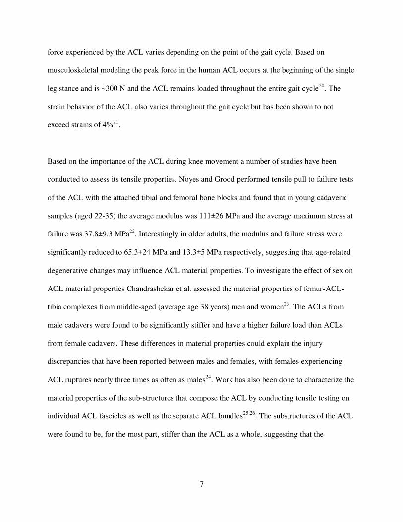
force experienced by the ACL varies depending on the point of the gait cycle. Based on

musculoskeletal modeling the peak force in the human ACL occurs at the beginning of the single

leg stance and is ~300 N and the ACL remains loaded throughout the entire gait cycle20. The

strain behavior of the ACL also varies throughout the gait cycle but has been shown to not

exceed strains of 4%21.

Based on the importance of the ACL during knee movement a number of studies have been

conducted to assess its tensile properties. Noyes and Grood performed tensile pull to failure tests

of the ACL with the attached tibial and femoral bone blocks and found that in young cadaveric

samples (aged 22-35) the average modulus was 111±26 MPa and the average maximum stress at

failure was 37.8±9.3 MPa22. Interestingly in older adults, the modulus and failure stress were

significantly reduced to 65.3+24 MPa and 13.3±5 MPa respectively, suggesting that age-related

degenerative changes may influence ACL material properties. To investigate the effect of sex on

ACL material properties Chandrashekar et al. assessed the material properties of femur-ACL-

tibia complexes from middle-aged (average age 38 years) men and women23. The ACLs from

male cadavers were found to be significantly stiffer and have a higher failure load than ACLs

from female cadavers. These differences in material properties could explain the injury

discrepancies that have been reported between males and females, with females experiencing

ACL ruptures nearly three times as often as males24. Work has also been done to characterize the

material properties of the sub-structures that compose the ACL by conducting tensile testing on

individual ACL fascicles as well as the separate ACL bundles25,26. The substructures of the ACL

were found to be, for the most part, stiffer than the ACL as a whole, suggesting that the

8

interactions between the substructures during whole tissue movement may alter the whole tissue

material properties25,26.

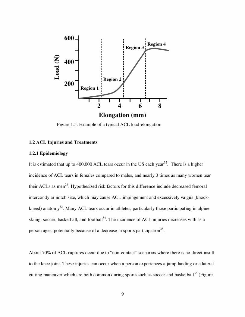
Similar to many other ligaments, the ACL possesses complex time-dependent viscoelastic

properties that are dependent on the collagen fibers and matrix materials, primarily elastin, that

compose the tissue27. The first region of the load-elongation curve is a linear region of low

stiffness where the elastin fibers are loaded and the collagen fibers are not yet engaged (Figure

1.5). The second region consists of a non-linear toe region where the collagen fibers are

beginning to undergo reversible un-crimping. In the third region of the loading curve the

collagen fibers are completely un-crimped and taut, which results in a constant higher stiffness28.

Finally, in the fourth region, the collagen fibers have ruptured and thus the stiffness increases

prior to complete failure. The time-dependent response of the ACL often manifests as creep,

change in the length of the ACL when exposed to a constant load, stress relaxation, a decrease in

measured load experienced by the ACL at a constant level of strain, and hysteresis, energy

dissipation with continual loading and unloading29,30. These viscoelastic properties are important

to take into consideration when assessing an appropriate replacement for a ruptured ACL since

the ideal replacement should have similar viscoelastic properties31.

9

1.2 ACL Injuries and Treatments

1.2.1 Epidemiology

It is estimated that up to 400,000 ACL tears occur in the US each year32. There is a higher

incidence of ACL tears in females compared to males, and nearly 3 times as many women tear

their ACLs as men24. Hypothesized risk factors for this difference include decreased femoral

intercondylar notch size, which may cause ACL impingement and excessively valgus (knock-

kneed) anatomy33. Many ACL tears occur in athletes, particularly those participating in alpine

skiing, soccer, basketball, and football34. The incidence of ACL injuries decreases with as a

person ages, potentially because of a decrease in sports participation35.

About 70% of ACL ruptures occur due to “non-contact” scenarios where there is no direct insult

to the knee joint. These injuries can occur when a person experiences a jump landing or a lateral

cutting maneuver which are both common during sports such as soccer and basketball36 (Figure

Figure 1.5: Example of a typical ACL load-elongation curve.

200

400

600

2 4 6 8

Region 1

Elongation (mm)

Load

(N

)

Region 2

Region 3Region 4

10

1.6). During a jump landing, a rupture of the ACL may occur when the knee is in a shallow state

of flexion and the tibia translates too far anteriorly, allowing the femur to begin to slide

posteriorly off the tibial plateau, rupturing the ACL (Figure 1.6A). Additionally, if a knee

undergoes simultaneous valgus and internal rotation of the tibia, such as during a cutting motion,

the combined loading mechanism could cause the ACL to rupture (Figure 1.6B). ACL ruptures

typically occur in conjunction with damage to the surrounding tissues, including the menisci,

cartilage, subchondral bone, and other knee ligaments37.

Figure 1.6: Examples of motions that frequently cause ACL ruptures: jump landing (A) and cutting movements (B). Reprinted with permission from Levine et al. 201336.

BA

11

Each year in the US between 100,000 and 400,000 patients undergo ACL surgeries32.

Additionally, because only one-third of ACL tears occur with no concomitant injuries, an ACL

rupture surgery often involves additional procedures38. For example, a study of patients in New

York State reported that 32% of all patients who underwent surgery for an ACL rupture also

required treatment of a meniscal injury, which increases surgical time and costs35. The cost of an

ACL surgery depends on a number of factors including the type of graft used, the source of the

graft, and graft processing. An ACL reconstruction using an autograft, where the graft is

harvested from the patient’s own body, typically costs $5,000-$6,000 and an ACL allograft,

where the graft is obtained from a donor, costs $6,000-$7,00039. Should a primary ACL graft

fail, a revision surgery is often even more expensive and can cost roughly $20,00040. Including

all surgical and rehabilitation costs, the estimate for treating ACL injuries in the use is $1.7

billion annually33.

1.2.2 Treatments and Outcomes

Rupture of the ACL results in significant alterations to knee joint kinematics. During normal

activities, a joint with a ruptured ACL often has an increased anterior translation of the tibia as

well as more internal tibial rotation15,16. Because the ACL is one of the primary joint stabilizers,

when it is ruptured the stabilizing role is transferred to the surrounding joint structures, including

the bone, cartilage, menisci, and other major ligaments such as the MCL and PCL41. The

alteration of knee kinematics and transition of load to surrounding tissues may cause the tissues

to be more susceptible to damage and degradation42. Thus, if left untreated, ACL ruptures often

lead to pain, feelings of instability, bone bruising and occult tissue damage. The prevalence of

12

radiographic knee osteoarthritis has been reported to be 60%-90% at 10-15 years after injury for

patients who receive conservative (i.e. non-surgical) treatment43–45.

The standard surgical treatment for an ACL rupture is to remove any remaining tissue and

reconstruct the ACL with a free tendon graft. The tendon graft is put in place through bone

tunnels in the femur and tibia and anchored at the bone ends. A number of factors associated

with the ACL reconstruction surgery including the placement of bone tunnels, the pre-tensioning

of the graft, the fixation method, and the fixation strength can vary among patients and may

significantly affect surgical outcomes46. The two most common types of ACL grafts are

autografts, where tissue is harvested from the patient, and allografts, where donor tissue is used.

For autografts, the most common choices are the patellar tendon with attached bone blocks or

semitendinosus-gracilis tendons. Bone-patellar tendon-bone grafts are advantageous because the

attached bone blocks allow for graft fixation within tibial and femoral bone tunnels which can

improve healing and stability47. However, meta-analyses have reported no significant differences

in clinical outcomes between patellar tendon and semitendinosus-gracilis tendon grafts48,49. The

major drawback to autografts is that the tissue must be harvested from the patients’ own body

which necessitates a second surgical site and can result in donor site morbidity, pain and muscle

weakness. In contrast, ACL allografts are tissues that are obtained from donor cadavers. Tendons

used for allografts include the semitendinosus tendon, the gracilis tendon, and the Achilles

tendon50 (Figure 1.7). The major drawback to allografts is that the physical and chemical

processing techniques used to sterilize and store the donor tissue may affect tissue integrity and

alter the material properties51. A meta-analysis found that when autograft and allograft bone-

13

patellar-bone grafts were compared, patients who received an allograft were more likely to

rupture the graft and score lower on functional tests52.

Regardless of reconstruction technique, at 10 years follow up, up to 13% of ACL reconstruction

patients display signs of radiographic knee osteoarthritis53. The prevalence of radiographic knee

osteoarthritis increases to 21%-48% if the ACL tear occurs in combination with an injury to the

meniscus54. Poor outcomes of ACL reconstruction may be attributed to failure to match the

material properties of the ACL, failure to restore normal joint kinematics or a lack of a biological

healing cascade55. Undesirable outcomes of traditional ACL surgical reconstruction techniques

have motivated research on alternative ACL repair and replacement strategies33.

1.3 ACL Tissue Engineering

Based on the drawbacks to traditional ACL allografts there has been interest in developing a

synthetic ACL replacement since the early 1970s. However, there are currently no FDA

Figure 1.7: Examples of ACL allografts: Semitendinosus tendon (top), gracilis tendon (middle), and Achilles tendon (bottom). Reprinted with permission from Cohen et al. 200750.

14

approved synthetic devices for primary ACL repair on the US market. Recent advancements in

our understanding of the life sciences have motivated researchers to focus on the development a

tissue engineered ACL replacement. Tissue engineering is a multidisciplinary field that

incorporates aspects of engineering, biology, chemistry, and materials science technique to create

replacements for damaged tissues56. The most common paradigm of tissue engineering is the use

of a scaffold, cells, and signaling molecules in combination to encourage the regeneration of new

tissue. Tissue engineering offers a unique opportunity to not repair damaged tissue but instead

engineer new, or de novo, tissue.

1.3.1 Scaffolds

The scaffolds utilized for tissue engineering applications provide mechanical stability and act as

a substrate for cell growth. When assessing scaffolds for use in ACL tissue engineering it is

important to consider the type of material as well as its mechanical and biochemical properties.

Due to the important mechanical function of the native ACL, a successful ACL scaffold must

have material properties that are comparable to the native ACL. Additionally, an appropriate

scaffold should have the ability to promote cellular attachment and encourage ligament tissue

growth and remodeling, while being compatible with the surrounding tissue and not provoking

an immune response. Finally, the degradation rate of the scaffold must be considered. Ideally, the

scaffold degradation rate should match the rate of new tissue formation.

Both xenogeneic materials, as well as other natural materials, have been considered for tissue

engineering scaffolds of ligamentous materials. Collagen, the primary component of the native

ACL, has been a popular choice for the creation of ACL scaffolds based on its biocompatibility

15

and the wide availability of xenogeneic (bovine) collagen. Despite promoting fibroblast

adhesion, collagen lacks mechanical strength and xenogeneic collagen can provoke an immune

response57,58. Silk is another natural polymer that has been investigated, primarily because of its

superior tensile strength. However in its natural state silk does not promote cell adhesion, and

chemical modification to increase cell attachment can modify the morphology and mechanical

properties of the scaffolds59,60. Challenges with the use of naturally occurring polymers have led

researchers to focus on scaffolds fabricated from synthetic biodegradable polymers. Depending

on the type of polymer chosen it is possible to tailor the scaffold mechanical properties,

degradation rate, and cellular response. Materials such as poly(glycolic acid), poly(ʟ-lactic acid)

and poly(lactic-co-glycolic acid) are common FDA approved materials that can be manufactured

into various configurations and promote cell adhesion, however, the degradation products are

highly acidic and there are issues with poor mechanical strength61–63.

Recently polycaprolactone (PCL) has received significant attention as a suitable scaffold

material. PCL is a semi-crystalline polyester that is composed of repeating subunits of the

monomer ε-caprolactone64. Several PCL based medical devices have received US Food and Drug

Administration approval, including sutures and drug delivery devices65,66. PCL has also been

thoroughly investigated as a tissue engineering substrate and has been used for tissue engineering

of skin, knee menisci, nerves, and bone67–70.

PCL degrades via a hydrolytic degradation process due to the presence of hydrolytically labile

aliphatic ester linkages. The degradation of PCL happens slowly (over a period of ~2-3 years)

and the degradation products are readily metabolized via the citric acid cycle64. The degradation

16

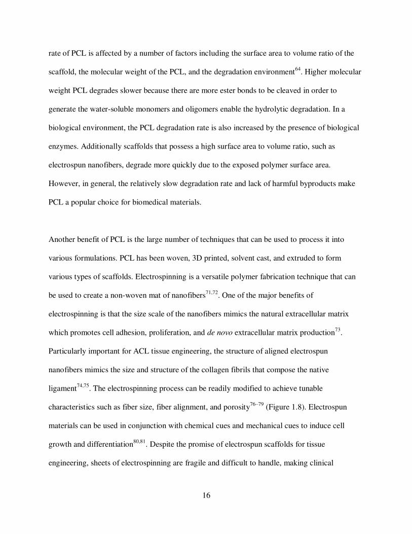
rate of PCL is affected by a number of factors including the surface area to volume ratio of the

scaffold, the molecular weight of the PCL, and the degradation environment64. Higher molecular

weight PCL degrades slower because there are more ester bonds to be cleaved in order to

generate the water-soluble monomers and oligomers enable the hydrolytic degradation. In a

biological environment, the PCL degradation rate is also increased by the presence of biological

enzymes. Additionally scaffolds that possess a high surface area to volume ratio, such as

electrospun nanofibers, degrade more quickly due to the exposed polymer surface area.

However, in general, the relatively slow degradation rate and lack of harmful byproducts make

PCL a popular choice for biomedical materials.

Another benefit of PCL is the large number of techniques that can be used to process it into

various formulations. PCL has been woven, 3D printed, solvent cast, and extruded to form

various types of scaffolds. Electrospinning is a versatile polymer fabrication technique that can

be used to create a non-woven mat of nanofibers71,72. One of the major benefits of

electrospinning is that the size scale of the nanofibers mimics the natural extracellular matrix

which promotes cell adhesion, proliferation, and de novo extracellular matrix production73.

Particularly important for ACL tissue engineering, the structure of aligned electrospun

nanofibers mimics the size and structure of the collagen fibrils that compose the native

ligament74,75. The electrospinning process can be readily modified to achieve tunable

characteristics such as fiber size, fiber alignment, and porosity76–79 (Figure 1.8). Electrospun

materials can be used in conjunction with chemical cues and mechanical cues to induce cell

growth and differentiation80,81. Despite the promise of electrospun scaffolds for tissue

engineering, sheets of electrospinning are fragile and difficult to handle, making clinical

17

translation difficult, and the mechanical properties are far inferior to the properties of native

ligaments. In an attempt to overcome these challenges several research groups are investigating

methods for creating more robust electrospun scaffolds using techniques such as braiding,

lamination and the inclusion of hydrogels82–84. With more complex scaffolds, encouraging cell

adhesion and proliferation while simultaneously achieving more robust mechanical properties

can be challenging.

1.3.2 Cells and Signaling Molecules

Another important consideration for ACL tissue engineering is the type of cell that is seeded

onto the scaffold. The ideal cell source is one that is readily available, has a high capacity for

proliferation, and has the ability to secrete de novo extracellular matrix material that mimics the

composition of the native ligament. In early tissue engineering attempts, primary ACL

Figure 1.8: Modifications of electrospun scaffolds: Altering nanofiber diameter (A, B), increasing pore spaces between fibers (C, D), and altering nanofiber alignment (E, F). Reprinted with permission from Balguid et al. 2009 (A, B)76, Baker et al. 2008 (C, D)77, and Ayres et al 2006 (E, F)79.

A B

C D

E F

20 µm 20 µm

20 µm 20 µm

50 µm 50 µm

18

fibroblasts were investigated as a cell source, since fibroblasts are the cells found in the native

ligament10. However, ACL fibroblasts are challenging to harvest and obtaining an adequate

number can be difficult. Once seeded on a scaffold ACL fibroblasts do produce collagen,

however, their low proliferative capacity limits usefulness85,86. More recent ACL tissue

engineering attempts have turned to pluripotent and multipotent stem cells. Bone marrow-

derived mesenchymal stems cells (BMSCs) are multipotent cells that can be derived from bone

marrow that has been harvested from long bones. BMSCs avoid the ethical challenges of

embryonic stems cells and can be directed to differentiate into a number of different types of

cells including chondrocytes, osteoblasts, and adipocytes87–89. In vitro and in vivo BMSCs have a

robust ability to proliferate and they are able to differentiate into fibroblasts and produce

collagen, which is vital for ligament tissue engineering applications85,90,91. Additionally, the use

of autologous BMSCs can eliminate potential issues with immune response after implantation.

Growth factors are chemical signaling molecules that are commonly used to influence cellular

activity. For ligament tissue engineering, growth factors are employed to increase cell

proliferation and extracellular matrix production. A number of growth factors, including

transforming growth factor beta (TGF-β), insulin-like growth factor (IGF), fibroblast growth

factor (FGF), and platelet-derived growth factor (PDGF), and have been shown to increase the

proliferative capacity and matrix production of ACL fibroblasts92–94. However, fewer studies

have been done to investigate the effects of ligament-related growth factors on BMSCs. In vitro,

FGF has been shown to increase BMSC proliferation, upregulate collagen production, and

encourage fibroblastic differentiation, however, the exact signaling pathway is unknown95,96.

Connective tissue growth factor (CTGF) is a heparin-binding protein that has also been shown to

19

encourage fibroblastic differentiation of stem cells as evidenced by increased cell proliferation,

alterations in gene expression, and increased ligament matrix deposition97,98.

When considering the type of growth factor to utilize for tissue engineering applications it is also

important to consider the method of growth factor delivery. The most common way to deliver

growth factors to cells is by including the growth factor in the in vitro cell culture media.

However, growth factors have a relatively short half-life in media and become rapidly

inactivated99. Sustained growth factor delivery is often necessary to influence cell behavior and

presents a challenge for creating functional scaffolds. Several strategies have been developed to

prolong the influence of growth factors on cells including physically incorporating the growth

factors into the bulk material of the scaffold and covalently conjugating growth factors onto

scaffold surfaces99. Covalent conjugation is a surface modification technique that utilizes

chemical bonds to immobilize growth factors to exposed functional groups on scaffold surfaces.

Typically, a chemical treatment is used to functionalize the nanofibers by the addition of

functional groups, and then a subsequent chemical treatment is used to covalently attach growth

factors (Figure 1.9). Growth factors conjugated to the surface scaffolds composed of electrospun

nanofibers have been utilized to encourage neuronal differentiation, enhance wound healing, and

stimulate osteogenic cellular activity80,100–102. Chemical conjugation of growth factors presents a

promising technique to allow growth factors to have a more extended influence on cells,

enabling prolonged increases in cell proliferation and ligament matrix production103.

20

1.4 Ovine Stifle Model

When assessing potential tissue engineered ligament replacements animal models are often used

for experimentation prior to human models. It is important to use an animal model that has

anatomical features comparable to those of the human knee joint. The sheep stifle joint anatomy

is similar to the anatomy of the human knee and prior work has shown that it is a valid surgical

model for the human knee104,105 (Figure 1.10). Additionally, sheep are relatively large compared

with most other animal models and the size of the stifle joint allows there to be adequate tissue

for mechanical, histological, and biochemical testing of the same joint. Previous groups have

successfully utilized the ovine stifle joint to study various orthopedic conditions and treatments

for the human knee joint, notably the development of osteoarthritis treatments and ligament

reconstruction techniques106–109.

Figure 1.9: Schematic of procedure for chemical conjugation of growth factors to electrospun nanofibers.

Electrospun nanofibersFunctionalized

electrospun nanofibers

Electrospun nanofibers with

conjugated growth factors

Chemical

treatment

Chemical

treatment

21

Due to the rising popularity of the ovine stifle joint as an orthopedic model, several research

groups have worked to thoroughly characterize the biomechanics of the joint. In ovine cadaver

stifles, tensile pull to failure tests have been conducted to assess the structural properties of the

native ACL. The mechanical properties of the native ovine ACL, including modulus, stiffness,

and load at failure, are comparable to the mechanical properties of the human ACL (Table

1)22,23,108,113. Compressive testing has been conducted to assess contact pressures and contact

areas on the tibial plateau of sheep during simulated gait and have shown that the tibiofemoral

contact pressures mimic what has been measured in the human knee110,112,114,115. In live sheep,

surgically implanted bone markers have been used to track the motion of the ovine stifle joint

during normal gait to assess the three-dimensional kinematics. During gait the ovine stifle

experiences flexion-extension angles between ~40º and ~80º which is a more narrow range of

angles and an overall more flexed position than what is observed during human gait115–118

(Figure 1.11). However, the peak tibiofemoral contact force during gait in sheep is ~2.12 times

Figure 1.10: Comparative anatomy of the human knee joint and the sheep stifle joint anterior aspect and tibial plateau. Reprinted with permission from Proffen et al. 2012105.

A B

C D

22

bodyweight, which is similar to the loads experienced by the human knee during gait115,119. The

anatomic similarity between the human knee joint and the ovine stifle joint and the thorough

characterization of the ovine stifle biomechanical properties make it an appropriate model for

investigating ACL replacements. Most notably the ovine stifle joint models offer an opportunity

to assess the ability of tissue engineered ACL scaffolds to mimic the hierarchal ACL structure,

encourage in vivo collagen deposition, possess appropriate tensile properties, and restore native

joint contact mechanics. A tissue-engineered scaffold that accomplishes these goals in the ovine

stifle joint could serve as an effective ACL replacement in the human knee joint.

Figure 1.11: Knee angle during ovine gait (A) and human gait (B) from heel strike (HS) to toe off (TO). Reprinted with permission from Tapper et al. 2008 (A)116 and Lafortune et al. 1992 (B)118.

A B

Table 1.1: Comparison of human and ovine ACL mechanical properties and tibiofemoral contact mechanics.

23

1.5 Specific Aims

The aim of this work is to develop a polymer scaffold to use as a replacement for the anterior

cruciate ligament (ACL). The scaffold should replicate the hierarchical structure of the native

ACL while possessing reasonable time-zero mechanical properties. In an in vitro environment,

the scaffold should encourage stem cell adhesion and proliferation and promote the deposition of

de novo ligament tissue, specifically collagen. Finally, the scaffold should be able to be

implanted in situ in an ovine stifle joint with standard surgical techniques and once implanted it

should adequately maintain tibiofemoral contact mecahnics during simulated joint loading.

Specific Aim 1: Fabricate and characterize an aligned 3-dimensional electrospun scaffold for

ACL replacement.

In order to provide a suitable replacement for a ruptured ligament, a scaffold should closely

match the structural and material properties of the native ACL. Based on the hierarchical

arrangement of collagen in the ACL a scaffold will be created to mimic the ligament structure

using the polymer polycaprolactone and the nanofiber fabrication technique electrospinning. The

subcomponents of the scaffold, flat sheets of electrospun nanofibers and rolled nanofiber bundles

will be tested via uniaxial tensile testing to determine the material properties. Adipose-derived

stem cells will be seeded on the scaffold subcomponents to assess the effect of the nanofiber

materials on cell adhesion, proliferation, and morphology.

Specific Aim 2: Assess the in vitro behavior of ovine bone marrow-derived stem cells seeded on

the scaffold in the presence of conjugated growth factor.

24

Once a scaffold has been created and characterized it is necessary to determine the in vitro cell

behavior in the presence of growth factors, signaling molecules used to induce the deposition of

collagen. Using a chemical conjugation technique connective tissue growth factor (CTGF) will

be covalently conjugated to the surface of nanofiber bundles and assessed for the conjugation

efficiency, growth factor release dynamics, conjugation efficiency, and the short-term response

of ovine bone-marrow derived stem cells (OBMSCs). The long-term response of OBMSCs will

be assessed using groups of ~20 nanofiber bundles conjugated with CTGF assembled together to

form a scaffold. Scaffolds will be evaluated for collagen production via histology, biochemical

assays, and immunohistochemistry.

Specific Aim 3: Evaluate the performance of the electrospun scaffold using uniaxial mechanical

testing.

A suitable ACL replacement must be surgically implantable and once implanted should mimic

the tensile properties of the intact ligament. First, a complete scaffold will be fabricated by

securing the ends of ~100 nanofiber bundles together with cylindrical solvent cast blocks of

PCL. The structural properties of the complete scaffold will be assessed via tensile mechanical

testing. Standard surgical techniques will be used to implant the scaffold into ovine cadaver stifle

joints in place of the native ACL. After scaffold implantation, the ovine cadaver stifle will be

assessed via tensile mechanical testing and a clinically relevant test of ACL integrity.

Mechanical behavior of the cadaver stifles with the implanted scaffold will be compared to knees

with the ACL intact and with a soft tissue graft ACL reconstruction.

25

Specific Aim 4: Assess the effect of the electrospun scaffold on ovine stifle joint contact

mechanics.

One of the primary functions of the ACL is to provide stability to the knee joint and thus

maintain a normal distribution of contact pressure between the femur and tibia. The tibiofemoral

contact mechanics of cadaver ovine stifle joints will be assessed during simulated gait angles

using thin film pressure sensors. Contact mechanics from four conditions will be assessed: (1)

the native ACL intact, (2) the native ACL transected, (3) the electrospun scaffold implanted, and

(4) a soft tissue graft implanted to determine if presence of the electrospun scaffold allows for

the maintenance of normal tibiofemoral contact pressure and areas.

26

REFERENCES

1. Makris, E. A., Hadidi, P. & Athanasiou, K. A. The knee meniscus: structure-function, pathophysiology, current repair techniques, and prospects for regeneration. Biomaterials 32, 7411–31 (2011).

2. Smith, B. A., Livesay, G. A. & Woo, S. L. Biology and biomechanics of the anterior cruciate ligament. Clin. Sports Med. 12, 637–70 (1993).

3. Dye, S. F. & Cannon, W. D. Anatomy and biomechanics of the anterior cruciate ligament. Clin. Sports Med. 7, 715–25 (1988).

4. Arnoczky, S. Anatomy of the anterior cruciate ligament. Clin. Orthop. Relat. Res. 172, 19–25 (1983).

5. Girgis, F. G., Marshall, J. L. & Monajem, A. The cruciate ligaments of the knee joint. Anatomical, functional and experimental analysis. Clin. Orthop. Relat. Res. 216–31 (1975).

6. Odensten, M. & Gillquist, J. Functional anatomy of the anterior cruciate ligament and a rationale for reconstruction. J. Bone Joint Surg. Am. 67, 257–62 (1985).

7. Lu, H. H. & Thomopoulos, S. Functional attachment of soft tissues to bone: development, healing, and tissue engineering. Annu. Rev. Biomed. Eng. 15, 201–26 (2013).

8. Thomopoulos, S., Williams, G. R., Gimbel, J. A., Favata, M. & Soslowsky, L. J. Variation of biomechanical, structural, and compositional properties along the tendon to bone insertion site. J. Orthop. Res. 21, 413–419 (2003).

9. Danylchuk, K. D., Finlay, J. B. & Krcek, J. P. Microstructural organization of human and bovine cruciate ligaments. Clin. Orthop. Relat. Res. 131, 294–298 (1978).

10. Duthon, V. B., Barea, C., Abrassart, S., Fasel, J. H., Fritschy, D. & Ménétrey, J. Anatomy of the anterior cruciate ligament. Knee Surg. Sports Traumatol. Arthrosc. 14, 204–13 (2006).

11. Amiel, D., Frank, C., Harwood, F., Fronek, J. & Akeson, W. Tendons and ligaments: a morphological and biochemical comparison. J. Orthop. Res. 1, 257–65 (1984).

12. Murray, M. M. & Spector, M. Fibroblast distribution in the anteromedial bundle of the human anterior cruciate ligament: The presence of alpha-smooth muscle actin-positive cells. J. Orthop. Res. 17, 18–27 (1999).

27

13. Schutte, M., Dabezies, E., Zimny, M. & Happel, L. Neural anatomy of the human anterior cruciate ligament. J. Bone Jt. Surg. 69, 243–247 (1987).

14. Schultz, R. A., Miller, D. C., Kerr, C. S. & Micheli, L. Mechanoreceptors in human cruciate ligaments. A histological study. J. Bone Joint Surg. Am. 66, 1072–6 (1984).

15. Butler, D., Noyes, N. & Grood, E. Ligamentous restraints to anterior drawer in the human knee : a biomechanical study. J. Bone Jt. Surg. 62, 259–270 (1980).

16. Beynnon, B., Fleming, B., Labovitch, R. & Parsons, B. Chronic anterior cruciate ligament deficiency is associated with increased anterior tranlslation of the tibia during the transition from non-weightbearing to weightbearing. J Orthop Res 20, 332–337 (2002).

17. Kondo, E., Merican, A. M., Yasuda, K. & Amis, A. A. Biomechanical Comparison of Anatomic Double-Bundle, Anatomic Single-Bundle, and Nonanatomic Single-Bundle Anterior Cruciate Ligament Reconstructions. Am. J. Sports Med. 39, 279–288 (2011).

18. Kim, S. J. & Kim, H. K. Reliability of the anterior drawer test, the pivot shift test, and the Lachman test. Clin. Orthop. Relat. Res. 237–242 (1995).

19. Katz, J. W. & Fingeroth, R. J. The diagnostic accuracy of ruptures of the anterior cruciate ligament comparing the Lachman test, the anterior drawer sign, and the pivot shift test in acute and chronic knee injuries. Am. J. Sports Med. 14, 88–91 (1986).

20. Shelburne, K. B., Pandy, M. G., Anderson, F. C. & Torry, M. R. Pattern of anterior cruciate ligament force in normal walking. J. Biomech. 37, 797–805 (2004).

21. Beynnon, B. D. & Fleming, B. C. Anterior cruciate ligament strain in-vivo: a review of previous work. J. Biomech. 31, 519–25 (1998).

22. Noyes, F. R. & Grood, E. S. The strength of the anterior cruciate ligament in humans and Rhesus monkeys. J. Bone Joint Surg. Am. 58, 1074–82 (1976).

23. Chandrashekar, N., Mansouri, H., Slauterbeck, J. & Hashemi, J. Sex-based differences in the tensile properties of the human anterior cruciate ligament. J. Biomech. 39, 2943–50 (2006).

24. Prodromos, C. C., Han, Y., Rogowski, J., Joyce, B. & Shi, K. A Meta-analysis of the Incidence of Anterior Cruciate Ligament Tears as a Function of Gender, Sport, and a Knee Injury-Reduction Regimen. Arthrosc. J. Arthrosc. Relat. Surg. 23, 1320–1325 (2007).

25. Butler, D. L., Guan, Y., Kay, M. D., Cummings, J. F., Feder, S. M. & Levy, M. S. Location-dependent variations in the material properties of the anterior cruciate ligament. J. Biomech. 25, 511–518 (1992).

28

26. Butler, D. L., Kay, M. D. & Stouffer, D. C. Comparison of material properties in fascicle-bone units from human patellar tendon and knee ligaments. J. Biomech. 19, 425–32 (1986).

27. Mow, V. C. & Hayes, W. C. Basic orthopaedic biomechanics. (New York: Raven Press, 1991).

28. Fratzl, P., Misof, K., Zizak, I., Rapp, G., Amenitsch, H. & Bernstorff, S. Fibrillar structure and mechanical properties of collagen. J. Struct. Biol. 122, 119–22 (1998).

29. Provenzano, P., Lakes, R., Keenan, T. & Vanderby, R. Nonlinear ligament viscoelasticity. Ann. Biomed. Eng. 29, 908–914 (2001).

30. Woo, S. L., Debski, R. E., Withrow, J. D. & Janaushek, M. A. Biomechanics of knee ligaments. Am. J. Sports Med. 27, 533–43 (1999).

31. Freeman, J. W., Woods, M. D., Cromer, D. a, Wright, L. D. & Laurencin, C. T. Tissue engineering of the anterior cruciate ligament: the viscoelastic behavior and cell viability of a novel braid-twist scaffold. J. Biomater. Sci. Polym. Ed. 20, 1709–1728 (2009).

32. Junkin, D., Johnson, D., Fu, F., Mark, M., Willenborn, M., Fanelli, G. & Wascher, D. in Orthop. Knowl. Updat. Sport. Med. 4 135–146 (American Academy of Orthopaedic Surgeons, 2009).

33. Kiapour, a M. & Murray, M. M. Basic science of anterior cruciate ligament injury and repair. Bone Joint Res. 3, 20–31 (2014).

34. Renstrom, P., Ljungqvist, A., Arendt, E., Beynnon, B., Fukubayashi, T., Garrett, W., Georgoulis, T., Hewett, T. E., Johnson, R., Krosshaug, T., Mandelbaum, B., Micheli, L., Myklebust, G., Roos, E., Roos, H., Schamasch, P., Shultz, S., Werner, S., Wojtys, E., Engebretsen, L. & Khan, K. Non-contact ACL injuries in female athletes: An International Olympic Committee current concepts statement. Br. J. Sport. Medi 41, 20–30 (2008).

35. Vavken, P. & Murray, M. M. Treating Anterior Cruciate Ligament Tears in Skeletally Immature Patients. Arthrosc. J. Arthrosc. Relat. Surg. 27, 704–716 (2011).

36. Levine, J. W., Kiapour, A. M., Quatman, C. E., Wordeman, S. C., Goel, V. K., Hewett, T. E. & Demetropoulos, C. K. Clinically relevant injury patterns after an anterior cruciate ligament injury provide insight into injury mechanisms. Am. J. Sports Med. 41, 385–95 (2013).

37. Beynnon, B. D., Johnson, R. J., Abate, J. a., Fleming, B. C. & Nichols, C. E. Treatment of Anterior Cruciate Ligament Injuries, Part I. Am. J. Sports Med. 33, 1579–1602 (2005).

38. Murray, M. M., Spindler, K. P., Devin, C., Snyder, B. S., Muller, J., Takahashi, M., Ballard, P., Nanney, L. B. & Zurakowski, D. Use of a collagen-platelet rich plasma

29

scaffold to stimulate healing of a central defect in the canine ACL. J. Orthop. Res. 24, 820–30 (2006).

39. Cooper, M. T. & Kaeding, C. Comparison of the hospital cost of autograft versus allograft soft-tissue anterior cruciate ligament reconstructions. Arthrosc. - J. Arthrosc. Relat. Surg. 26, 1478–1482 (2010).

40. Genuario, J. W., Faucett, S. C., Boublik, M. & Schlegel, T. F. A Cost-Effectiveness Analysis Comparing 3 Anterior Cruciate Ligament Graft Types. Am. J. Sports Med. 40, 307–314 (2012).

41. Noyes, F., Mooar, P., Matthews, D. & Butler, D. The symptomatic anterior cruciate-deficient knee. Part I: The long-term functional disability in athletically active individuals. J. Bone Jt. Surg. 65, 154–62 (1983).

42. Bray, R. C. & Dandy, D. J. Meniscal lesions and chronic anterior cruciate ligament deficiency. Meniscal tears occurring before and after reconstruction. J. Bone Joint Surg.

Br. 71, 128–30 (1989).

43. Sommerlath, K., Lysholm, J. & Gillquist, J. The long-term course after treatment of acute anterior cruciate ligament ruptures: A 9 to 16 year followup. Am. J. Sports Med. 19, 156–162 (1991).

44. Nebelung, W. & Wuschech, H. Thirty-five years of follow-up of anterior cruciate ligament - Deficient knees in high-level athletes. Arthrosc. - J. Arthrosc. Relat. Surg. 21, 696–702 (2005).

45. Gillquist, J. & Messner, K. Anterior cruciate ligament reconstruction and the long-term incidence of gonarthrosis. Sports Med. 27, 143–156 (1999).

46. Dargel, J., Gotter, M., Mader, K., Pennig, D., Koebke, J. & Schmidt-Wiethoff, R. Biomechanics of the anterior cruciate ligament and implications for surgical reconstruction. Strateg. Trauma Limb Reconstr. 2, 1–12 (2007).

47. Woo, S. L.-Y., Wu, C., Dede, O., Vercillo, F. & Noorani, S. Biomechanics and anterior cruciate ligament reconstruction. J. Orthop. Surg. Res. 1, 1–9 (2006).

48. Biau, D., Tournoux, C., Katsahian, S., Schranz, P. & Nizard, R. Bone-patellar tendon-bone autografts versus hamstring autografts for reconstruction of anterior cruciate ligament: meta-analysis. BMJ 332, 995–1001 (2006).

49. Biau, D. J., Tournoux, C., Katsahian, S., Schranz, P. & Nizard, R. ACL Reconstruction. Clin. Orthop. Relat. Res. 180–187 (2007).

50. Cohen, S. B. & Sekiya, J. K. Allograft Safety in Anterior Cruciate Ligament Reconstruction. Clin. Sports Med. 26, 597–605 (2007).

30

51. Sun, K., Tian, S., Zhang, J., Xia, C., Zhang, C. & Yu, T. Anterior cruciate ligament reconstruction with BPTB autograft, irradiated versus non-irradiated allograft: A prospective randomized clinical study. Knee Surgery, Sport. Traumatol. Arthrosc. 17, 464–474 (2009).

52. Krych, A. J., Jackson, J. D., Hoskin, T. L. & Dahm, D. L. A Meta-analysis of Patellar Tendon Autograft Versus Patellar Tendon Allograft in Anterior Cruciate Ligament Reconstruction. Arthrosc. J. Arthrosc. Relat. Surg. 24, 292–298 (2008).

53. Lohmander, L. S., Ostenberg, a, Englund, M. & Roos, H. High prevalence of knee osteoarthritis, pain, and functional limitations in female soccer players twelve years after anterior cruciate ligament injury. Arthritis Rheum. 50, 3145–52 (2004).

54. Øiestad, B. E., Holm, I., Aune, A. K., Gunderson, R., Myklebust, G., Engebretsen, L., Fosdahl, M. A. & Risberg, M. A. Knee Function and Prevalence of Knee Osteoarthritis After Anterior Cruciate Ligament Reconstruction. Am. J. Sports Med. 38, 2201–2210 (2010).

55. Domnick, C., Raschke, M. J. & Herbort, M. Biomechanics of the anterior cruciate ligament: Physiology, rupture and reconstruction techniques. World J. Orthop. 7, 82–93 (2016).

56. Langer, R. & Vacanti, J. Tissue engineering. Science. 260, 920–926 (1993).

57. Dunn, M. G., Liesch, J. B., Tiku, M. L. & Zawadsky, J. P. Development of fibroblast-seeded ligament analogs for ACL reconstruction. J. Biomed. Mater. Res. 29, 1363–1371 (1995).

58. Bellincampi, L. D., Closkey, R. F., Prasad, R., Zawadsky, J. P. & Dunn, M. G. Viability of fibroblast-seeded ligament analogs after autogenous implantation. J. Orthop. Res. 16, 414–420 (1998).

59. Altman, G. H., Horan, R. L., Martin, I., Farhadi, J., Stark, P. R. H., Volloch, V., Richmond, J. C., Vunjak-Novakovic, G. & Kaplan, D. L. Cell differentiation by mechanical stress. FASEB J. 16, 270–2 (2002).

60. Fan, H., Liu, H., Toh, S. L. & Goh, J. C. H. Anterior cruciate ligament regeneration using mesenchymal stem cells and silk scaffold in large animal model. Biomaterials 30, 4967–4977 (2009).

61. Lin, V. S., Lee, M. C., O’Neal, S., McKean, J. & Sung, K.-L. P. Ligament Tissue Engineering Using Synthetic Biodegradable Fiber Scaffolds. Tissue Eng. 5, 443–451 (1999).

31

62. Lu, H. H., Cooper, J. A., Manuel, S., Freeman, J. W., Attawia, M. A., Ko, F. K. & Laurencin, C. T. Anterior cruciate ligament regeneration using braided biodegradable scaffolds: in vitro optimization studies. Biomaterials 26, 4805–16 (2005).

63. Chen, G., Sato, T., Sakane, M., Ohgushi, H., Ushida, T., Tanaka, J. & Tateishi, T. Application of PLGA-collagen hybrid mesh for three-dimensional culture of canine anterior cruciate ligament cells. Mater. Sci. Eng. C 24, 861–866 (2004).

64. Woodruff, M. A. & Hutmacher, D. W. The return of a forgotten polymer—Polycaprolactone in the 21st century. Prog. Polym. Sci. 35, 1217–1256 (2010).

65. Bezwada, R. S., Jamiolkowski, D. D., Lee, I. Y., Agarwal, V., Persivale, J., Trenka-Benthin, S., Erneta, M., Suryadevara, J., Yang, A. & Liu, S. Monocryl suture, a new ultra-pliable absorbable monofilament suture. Biomaterials 16, 1141–1148 (1995).

66. Darney, P. D., Monroe, S. E., Klaisle, C. M. & Alvarado, A. Clinical evaluation of the Capronor contraceptive implant: Preliminary report. Am. J. Obstet. Gynecol. 160, 1292–1295 (1989).

67. Chiari, C., Koller, U., Dorotka, R., Eder, C., Plasenzotti, R., Lang, S., Ambrosio, L., Tognana, E., Kon, E., Salter, D. & Nehrer, S. A tissue engineering approach to meniscus regeneration in a sheep model. Osteoarthr. Cartil. 14, 1056–1065 (2006).

68. Ng, K. W., Hutmacher, D. W., Schantz, J. T., Ng, C. S., Too, H. P., Lim, T. C., Phan, T. T. & Teoh, S. H. Evaluation of Ultra-Thin Poly(ε-Caprolactone) Films for Tissue-Engineered Skin. Tissue Eng. 7, 441–455 (2001).

69. Koshimune, M., Takamatsu, K., Nakatsuka, H., Inui, K., Yamano, Y. & Ikada, Y. Creating bioabsorbable Schwann cell coated conduits through tissue engineering. Biomed.

Mater. Eng. 13, 223–229 (2003).

70. Chuenjitkuntaworn, B., Inrung, W., Damrongsri, D., Mekaapiruk, K., Supaphol, P. & Pavasant, P. Polycaprolactone/hydroxyapatite composite scaffolds: Preparation, characterization, and in vitro and in vivo biological responses of human primary bone cells. J. Biomed. Mater. Res. - Part A 94, 241–251 (2010).

71. Li, D. & Xia, Y. Electrospinning of Nanofibers: Reinventing the Wheel? Adv. Mater. 16, 1151–1170 (2004).

72. Pedicini, A. & Farris, R. J. Mechanical behavior of electrospun polyurethane. Polymer. 44, 6857–6862 (2003).

73. Pham, Q. P., Sharma, U. & Mikos, A. G. Electrospinning of polymeric nanofibers for tissue engineering applications: a review. Tissue Eng. 12, 1197–211 (2006).

32

74. Choi, J. S., Lee, S. J., Christ, G. J., Atala, A. & Yoo, J. J. The influence of electrospun aligned poly(e-caprolactone)/collagen nanofiber meshes on the formation of self-aligned skeletal muscle myotubes. Biomaterials 29, 2899–2906 (2008).

75. Li, W. J., Mauck, R. L., Cooper, J. a, Yuan, X. & Tuan, R. S. Engineering controllable anisotropy in electrospun biodegradable nanofibrous scaffolds for musculoskeletal tissue engineering. J. Biomech. 40, 1686–93 (2007).

76. Balguid, A., Mol, A., Van Marion, M. H., Bank, R. A., Bouten, C. V. C. & Baaijens, F. P. T. Tailoring fiber diameter in electrospun poly(epsilon-caprolactone) scaffolds for optimal cellular infiltration in cardiovascular tissue engineering. Tissue Eng. Part A 15, 437–44 (2009).

77. Baker, B. M., Gee, A. O., Metter, R. B., Nathan, A. S., Marklein, R. a, Burdick, J. a & Mauck, R. L. The potential to improve cell infiltration in composite fiber-aligned electrospun scaffolds by the selective removal of sacrificial fibers. Biomaterials 29, 2348–58 (2008).

78. Wang, K., Zhu, M., Li, T., Zheng, W., Xu, L. L., Zhao, Q., Kong, D. & Wang, L. Improvement of Cell Infiltration in Electrospun Polycaprolactone Scaffolds for the Construction of Vascular Grafts. J. Biomed. Nanotechnol. 10, 1588–1598 (2014).

79. Ayres, C., Bowlin, G. L., Henderson, S. C., Taylor, L., Shultz, J., Alexander, J., Telemeco, T. A. & Simpson, D. G. Modulation of anisotropy in electrospun tissue-engineering scaffolds: Analysis of fiber alignment by the fast Fourier transform. Biomaterials 27, 5524–34 (2006).

80. Cho, Y. Il, Choi, J. S., Jeong, S. Y. & Yoo, H. S. Nerve growth factor (NGF)-conjugated electrospun nanostructures with topographical cues for neuronal differentiation of mesenchymal stem cells. Acta Biomater. 6, 4725–4733 (2010).

81. Sahoo, S., Ang, L. T., Goh, J. C. H. & Toh, S. L. Growth factor delivery through electrospun nanofibers in scaffolds for tissue engineering applications. J. Biomed. Mater.

Res. A 93, 1539–1550 (2010).

82. Barber, J. G., Handorf, A. M., Allee, T. J. & Li, W.-J. Braided nanofibrous scaffold for tendon and ligament tissue engineering. Tissue Eng. Part A 19, 1265–74 (2013).

83. Petrigliano, F. A., Arom, G. A., Nazemi, A. N., Yeranosian, M. G., Wu, B. M. & McAllister, D. R. In Vivo Evaluation of Electrospun Polycaprolactone Graft for Anterior Cruciate Ligament Engineering. Tissue Eng. Part A 21, 1228–2136 (2015).

84. Xu, W., Ma, J. & Jabbari, E. Material properties and osteogenic differentiation of marrow stromal cells on fiber-reinforced laminated hydrogel nanocomposites. Acta Biomater. 6, 1992–2002 (2010).

33

85. Van Eijk, F., Saris, D. B. F., Riesle, J., Willems, W. J., Van Blitterswijk, C. a., Verbout, a. J. & Dhert, W. J. a. Tissue engineering of ligaments: a comparison of bone marrow stromal cells, anterior cruciate ligament, and skin fibroblasts as cell source. Tissue Eng. 10, 893–903 (2004).

86. Liu, H., Fan, H., Toh, S. L. & Goh, J. C. H. A comparison of rabbit mesenchymal stem cells and anterior cruciate ligament fibroblasts responses on combined silk scaffolds. Biomaterials 29, 1443–1453 (2008).

87. Caplan, A. I. Mesenchymal stem cells. J. Orthop. Res. 9, 641–50 (1991).

88. Jaiswal, N., Haynesworth, S. E., Caplan, a I. & Bruder, S. P. Osteogenic differentiation of purified, culture-expanded human mesenchymal stem cells in vitro. J. Cell. Biochem. 64, 295–312 (1997).

89. Dennis, J. E., Merriam, A., Awadallah, A., Yoo, J. U., Johnstone, B. & Caplan, A. I. A Quadripotential Mesenchymal Progenitor Cell Isolated from the Marrow of an Adult Mouse. J. Bone Miner. Res. 14, 700–709 (1999).

90. Vunjak-Novakovic, G., Altman, G., Horan, R. & Kaplan, D. L. Tissue engineering of ligaments. Annu. Rev. Biomed. Eng. 6, 131–56 (2004).

91. Fan, H., Liu, H., Wong, E. J. W., Toh, S. L. & Goh, J. C. H. In vivo study of anterior cruciate ligament regeneration using mesenchymal stem cells and silk scaffold. Biomaterials 29, 3324–37 (2008).

92. Meaney Murray, M., Rice, K., Wright, R. J. & Spector, M. The effect of selected growth factors on human anterior cruciate ligament cell interactions with a three-dimensional collagen-GAG scaffold. J. Orthop. Res. 21, 238–44 (2003).

93. Amiel, D., Nagineni, C. & Lee, J. Intrinsic properties of ACL and MCL cells and their responses to growth factors. Med. Sci. Sports Exerc. 27, 844–851 (1995).

94. Steinert, A. F., Weber, M., Kunz, M., Palmer, G. D., Nöth, U., Evans, C. H. & Murray, M. M. In situ IGF-1 gene delivery to cells emerging from the injured anterior cruciate ligament. Biomaterials 29, 904–916 (2008).

95. Hankemeier, S., Keus, M., Zeichen, J., Jagodzinski, M., Barkhausen, T., Bosch, U., Krettek, C. & Van Griensven, M. Modulation of proliferation and differentiation of human bone marrow stromal cells by fibroblast growth factor 2: potential implications for tissue engineering of tendons and ligaments. Tissue Eng. 11, 41–49 (2005).

96. Sahoo, S., Toh, S. L. & Goh, J. C. H. A bFGF-releasing silk/PLGA-based biohybrid scaffold for ligament/tendon tissue engineering using mesenchymal progenitor cells. Biomaterials 31, 2990–2998 (2010).

34

97. Lee, C. H., Shah, B., Moioli, E. K. & Mao, J. J. CTGF directs fibroblast differentiation from human mesenchymal stem/stromal cells and defines connective tissue healing in a rodent injury model. J. Clin. Invest. 120, 3340–3349 (2010).

98. Tong, Z., Sant, S., Khademhosseini, A. & Jia, X. Controlling the Fibroblastic Differentiation of Mesenchymal Stem Cells Via the Combination of Fibrous Scaffolds and Connective Tissue Growth Factor. Tissue Eng. Part A 17, 2773–2785 (2011).

99. Lee, K., Silva, E. A. & Mooney, D. J. Growth factor delivery-based tissue engineering: general approaches and a review of recent developments. J. R. Soc. Interface 8, 153–70 (2011).

100. Choi, J. S., Leong, K. W. & Yoo, H. S. In vivo wound healing of diabetic ulcers using electrospun nanofibers immobilized with human epidermal growth factor (EGF). Biomaterials 29, 587–596 (2008).

101. Mottaghitalab, F., Farokhi, M., Mottaghitalab, V., Ziabari, M., Divsalar, A. & Shokrgozar, M. A. Enhancement of neural cell lines proliferation using nano-structured chitosan/poly(vinyl alcohol) scaffolds conjugated with nerve growth factor. Carbohydr.

Polym. 86, 526–535 (2011).

102. Zhang, H., Migneco, F., Lin, C. Y. & Hollister, S. J. Chemically-conjugated bone morphogenetic protein-2 on three-dimensional polycaprolactone scaffolds stimulates osteogenic activity in bone marrow stromal cells. Tissue Eng. Part A 16, 3441–8 (2010).

103. Yoo, H. S., Kim, T. G. & Park, T. G. Surface-functionalized electrospun nanofibers for tissue engineering and drug delivery. Adv. Drug Deliv. Rev. 61, 1033–1042 (2009).

104. Allen, M. J., Houlton, J. E., Adams, S. B. & Rushton, N. The surgical anatomy of the stifle joint in sheep. Vet. Surg. VS Off. J. Am. Coll. Vet. Surg. 27, 596–605 (1998).

105. Proffen, B. L., McElfresh, M., Fleming, B. C. & Murray, M. M. A comparative anatomical study of the human knee and six animal species. Knee 19, 493–9 (2012).

106. Lu, Y., Markel, M. D., Nemke, B., Wynn, S. & Graf, B. Comparison of Single-Versus Double-Tunnel Tendon-to-Bone Healing in an Ovine Model: A Biomechanical and Histological Analysis. Am. J. Sports Med. 37, 512–517 (2009).

107. Ma, J., Smietana, M. J., Kostrominova, T. Y., Wojtys, E. M., Larkin, L. M. & Arruda, E. M. Three-dimensional engineered bone-ligament-bone constructs for anterior cruciate ligament replacement. Tissue Eng. Part A 18, 103–16 (2012).

108. Weiler, A., Peine, R., Pashmineh-Azar, A., Abel, C., Südkamp, N. P. & Hoffmann, R. F. G. Tendon healing in a bone tunnel. Part I: Biomechanical results after biodegradable interference fit fixation in a model of anterior cruciate ligament reconstruction in sheep. Arthroscopy 18, 113–123 (2002).

35

109. Oakley, S. P., Lassere, M. N., Portek, I., Szomor, Z., Ghosh, P., Kirkham, B. W., Murrell, G. a C., Wulf, S. & Appleyard, R. C. Biomechanical, histologic and macroscopic assessment of articular cartilage in a sheep model of osteoarthritis. Osteoarthr. Cartil. 12, 667–679 (2004).

110. Morimoto, Y., Ferretti, M., Ekdahl, M., Smolinski, P. & Fu, F. H. Tibiofemoral Joint Contact Area and Pressure After Single- and Double-Bundle Anterior Cruciate Ligament Reconstruction. Arthrosc. - J. Arthrosc. Relat. Surg. 25, 62–69 (2009).

111. Mahalingam, V., Wojtys, E. M., Wellik, D. M., Arruda, E. M. & Larkin, L. M. Fresh and Frozen Tissue-Engineered Three-Dimensional Bone–Ligament–Bone Constructs for Sheep Anterior Cruciate Ligament Repair Following a 2-Year Implantation. Biores. Open

Access 5, 289–298 (2016).

112. Lee-Shee, N. K., Dickey, J. P. & Hurtig, B. Contact mechanics of the ovine stifle during simulated early stance in gait: An in vitro study using robotics. Vet. Comp. Orthop.

Traumatol. 20, 70–72 (2007).

113. Scheffler, S. U., Schmidt, T., Gangéy, I., Dustmann, M., Unterhauser, F. & Weiler, A. Fresh-Frozen Free-Tendon Allografts Versus Autografts in Anterior Cruciate Ligament Reconstruction: Delayed Remodeling and Inferior Mechanical Function During Long-term Healing in Sheep. Arthrosc. - J. Arthrosc. Relat. Surg. 24, 448–458 (2008).

114. Bedi, A., Chen, T., Santner, T. J., El Amin, S., Kelly, N. H., Warren, R. F. & Maher, S. a. Changes in dynamic medial tibiofemoral contact mechanics and kinematics after injury of the anterior cruciate ligament: A cadaveric model. Proc. Inst. Mech. Eng. Part H J. Eng.

Med. 227, 1027–1037 (2014).

115. Taylor, W. R., Ehrig, R. M., Heller, M. O., Schell, H., Seebeck, P. & Duda, G. N. Tibio-femoral joint contact forces in sheep. J. Biomech. 39, 791–798 (2006).

116. Tapper, J. E., Fukushima, S., Azuma, H., Sutherland, C., Marchuk, L., Thornton, G. M., Ronsky, J. L., Zernicke, R., Shrive, N. G. & Frank, C. B. Dynamic in vivo three-dimensional (3D) kinematics of the anterior cruciate ligament/medial collateral ligament transected ovine stifle joint. J. Orthop. Res. 26, 660–672 (2008).

117. Winter, D. A. Kinematic and kinetic patterns in human gait: Variability and compensating effects. Hum. Mov. Sci. 3, 51–76 (1984).

118. Lafortune, M. A., Cavanagh, P. R., Sommer, H. J. & Kalenak, A. Three-dimensional kinematics of the human knee during walking. J. Biomech. 25, 347–357 (1992).

119. Hardt, D. E. Determining muscle forces in the leg during normal human walking - An application and evaluation of optimization methods. J. Biomech. Eng. 100, 72–78 (1978).

36

CHAPTER 2:

MECHANICAL PROPERTIES AND CELLULAR RESPONSE OF NOVEL

ELECTROSPUN NANOFIBERS FOR LIGAMENT TISSUE ENGINEERING: EFFECTS

OF ORIENTATION AND GEOMETRY1

2.1 Introduction

The high incidence of tendon and ligament injuries necessitates the need for an efficient repair

strategy. The anterior cruciate ligament (ACL) is frequently ruptured due to traumatic loading,

and in the United States alone up to 200,000 ACL tears occur annually 1,2. The most commonly

injured tendons include the flexor/extensor tendons of the hand (incidence of 4.83 and

18/100,000 per year respectively) and the Achilles tendon (12/100,000) 3. Following injury,

tendons and ligaments have a low intrinsic healing capacity due to limited vascularization and

thus surgery is required to repair or replace the injured tissue 4,5. The most common surgical

treatment options for tendon and ligament injuries are tissue replacement with allografts or

autografts. Although autografts have been historically successful, the primary drawback

associated with the technique is donor site morbidity that can result in pain, tendonitis, and

weakness 6,7. To avoid the complications associated with donor site morbidity, cadaver allografts

have been used as a primary repair technique; however, limited tissue supply and a risk of

disease transmission remain problematic 8. Regardless of the type of surgical intervention,

traumatic and degenerative tendon and ligament injuries still often lead to the development of

osteoarthritis 9,10.

1 This chapter has been published as a Research Paper in the Journal of the Mechanical Behavior of Biomedical Materials (61, 2016). All content has been adapted with permission from Elsevier.

37

In order to improve surgical outcomes of tendon and ligament repairs, the field of tissue

engineering has attempted to recapitulate the structure and function of the tendons and ligaments

to create an artificial replacement tissue. However, there are currently no FDA approved tissue

engineered tendon and ligament replacements 11. To successfully replace native tendons and

ligaments, biocompatibility and mechanical properties of the replacement should be considered

12. Collagen scaffolds are advantageous because collagen is a major component of the native

tendons and ligaments, however, these scaffolds lack sufficient mechanical strength and may

elicit an immune response 13,14. Silk scaffolds have superior mechanical properties but suffer

from limited cell attachment without extensive chemical modification 15,16. Synthetic polymers

are a popular option for scaffolds since many have already been FDA approved for other

applications 11. Biodegradable polymers can be utilized with a variety of fabrication techniques

and the characteristics of the resulting scaffold, including degradation rate, cell compatibility,

and mechanical properties, can be altered depending on the type of polymer used 12.

Tissue-engineered replacements should take into account the unique structure and mechanical

functions of tendons and ligaments which enables them to bear loads throughout complex joint

loading regimes. The smallest structural unit of tendons and ligaments are aligned collagen

fibrils, which range from 50-500 nm in diameter 4,17. Collagen fibrils are organized into fibers

approximately 10-50 μm in diameter. Groups of fibers are then organized into fascicles,

approximately 50-500 μm in size, which are combined to compose the whole tendon or ligament.

This hierarchical structure is likely important for the proper mechanical function of the tissue. It

is generally thought that tissue engineering strategies employed to recreate tendons and

38

ligaments must be able to accurately recapitulate complex the micro- and nano-scale structure in

order to achieve proper function 18,19.

Electrospinning is a versatile tissue engineering technique that results in a non-woven mat of

polymeric nanofibers 20,21. One of the major benefits of electrospinning is the ability to produce

nanofibers that may mimic the natural extracellular matrix of tissues, and thus can support cell

adhesion, proliferation, and extracellular matrix production 22. Furthermore, the structure of

aligned electrospun nanofibers mimic the dimensionality of collagen fibrils that comprise native

tendons and ligaments 23,24. Electrospinning can be readily modified to achieve tunable

characteristics such as fiber size, fiber alignment, and porosity 25–28. Despite the promise of

electrospun scaffolds in the field of tissue engineering, there are a number of factors that have

thus far limited their clinical applicability. Primarily, sheets of electrospun fibers are fragile and

difficult to handle, making them difficult to use in a clinical setting despite architectural

modifications in an attempt to improve handleability. Braided electrospun scaffolds seeded with

human bone marrow-derived stem cells have been shown to support cell adhesion and the

upregulation of tenogenic markers 29,30, and stacked electrospun scaffolds with laser cut pores

have successfully encouraged cell infiltration 31, but both demonstrated inferior mechanical

strength compared to native ligaments.

Since previous attempts have been unable to achieve the cellular and mechanical behavior

required for tendon and ligament replacement, it has become necessary to develop a more robust

electrospun construct, while still maintaining the complex structure and the cellular

compatibility. The hierarchical structure of tendons and ligaments has motivated the

39

development of micro-scale bundles of nanofibers, which mimic the fascicles that compose

native connective tissues. The objective of the following study was to assess the influence of

nanofiber orientation on mechanical properties and cellular response of nanofiber bundles that

have been designed to mimic the hierarchical organization of native tendons and ligaments. The

overarching goal of this work is to create a more robust tissue engineered tendon and ligament

replacement that closely replicates the native tissue structure.

2.2 Experimental Materials and Methods

2.2.1 Fabrication of nanofiber sheet and bundles

Poly(ε-caprolactone) (PCL) nanofiber sheets were fabricated using an electrospinning technique.

The solution for electrospinning was prepared by dissolving PCL pellets (Mw = 80,000, Sigma

440744, St. Louis, MO) in chloroform and mixing the polymer solution with oleic acid sodium

salt (OLA, TCI America O0057, Portland, OR) dissolved in methanol to ensure uniform fiber

diameter. The final 10% PCL electrospinning solution was a homogenous mixture with a 3:1

chloroform to methanol volume ratio and a 97:3 PCL to OLA ratio of the solid portion. For

electrospinning, a glass syringe (Cadence Scientific Micro-Mate, Staunton, VA) outfitted with an

18 gauge luer-lock blunt tip syringe needle (Hamilton 90134, Reno, NV) was filled with polymer

solution and situated within an adjustable flow syringe pump (Genie Touch, Kent Scientific,

Torrington, CT). The positive lead of a high voltage power supply (Acopian P030HP2, Easton,

PA) was connected to the needle tip with an alligator clip. The collector consisted of an

aluminum drum (NaBond, Shenzhen, China) 75 mm in diameter positioned 10 cm from the tip of

the syringe needle and covered in aluminum foil. To create a randomly oriented flat sheet of

nanofibers (Figure 2.1a) the collector drum was rotated at a speed of 300 rpm (linear velocity of

40

0.785 m/s), and to create a longitudinally aligned flat sheet of nanofibers (Figure 2.1b) the drum

was rotated at a speed of 3000 rpm (linear velocity of 23.6 m/s). The volumetric flow rate of the

PCL solution from the needle was 2.5 mL/h and the applied voltage was 15 kV. After fabricating

a flat nanofiber sheet, nanofiber bundles were created by excising a rectangular section

(approximately 5 cm x 10 cm) of either the random or aligned nanofiber sheet and rolling it into

a cylindrical bundle composed of nanofibers (Figure 2.1c). The fabrication of nanofiber bundles

required no special tools and was analogous to tightly rolling up a sheet of paper into a tube.

However, because the nanofiber sheets were very thin the center of the nanofiber bundle was not

hollow. This fabrication technique allowed for the fiber architecture and the pores between the

fibers to remain intact. After fabrication, the nanofiber sheets and bundles were soaked in

methanol for 24 h to remove any remaining OLA and stored in a desiccator until use.

Figure 2.1: Nanofiber sheets with random (a) and aligned (b) nanofibers were used to fabricate nanofiber bundles (c). The diameters of nanofibers which compose random and aligned nanofiber sheets are significantly different (d, * indicates p<0.05) however the diameter of random and aligned nanofiber bundles (NFB) are not significantly different e). Randomly oriented nanofiber sheets have a wider spread of nanofiber angles (f) compared to aligned nanofiber sheets (g).

41

2.2.2 Characterization of nanofiber sheets and bundles

Nanofiber sheets and bundles were mounted on stubs using carbon tape, sputter coated with a 10

nm thick gold coating, and imaged using a field emission scanning electron microscope (SEM,

JEOL JSM-6500F, Peabody, MA) operating at 10 kV to examine nanofiber architecture. To

quantify nanofiber diameter using SEM images, 5000x magnification images (n=6) were taken

from different samples of random and aligned nanofibers. Using Image J v1.48 (NIH, Bethesda,

MD), the diameter of 20 nanofibers in each image was manually (LG) measured. Diameters of

random and aligned nanofiber bundles (n=15) were quantified by imaging samples with a CCD

camera (Flea3, Point Grey Research, Richmond, BC, Canada) and measured manually.

The same 20 nanofibers used for diameter measurement were assessed for angular orientation to

quantify nanofiber alignment 32. A reference line was drawn along the horizontal plane and the

angle of each fiber was measured relative to the reference line. To account for initial rotation of

aligned samples the angles were normalized to the primary direction of sample rotation. The

analysis yielded a distribution of fiber angles ranging from -90° to 90° where 0° was defined as

the horizontal. Histograms were created from all angle measurements for both random and

aligned samples. Angular deviation was calculated using the MATLAB circular statistics toolbox

33.

Cross-sectional area of nanofiber sheets and bundles was determined two ways - via

measurements of “as-spun” nanofiber sheets and bundles with pores spaces left intact (Figure

2.2a, 2.2b), and of “compressed” nanofiber sheets and bundles with pores spaces removed

(Figure 2.2c, 2.2d). As-spun nanofiber sheets are highly porous and using sample width and

42

thickness to calculate cross-sectional area overestimates the true amount of material present in

the sample since the pores contribute significantly to the sample thickness. For nanofiber

bundles, using the outer diameter to calculate cross-sectional area does not take into account pore

space between nanofibers and additionally does not take into account any gaps between the

rolled “layers” of nanofiber sheets.

As-spun thickness of nanofiber sheets (n=5) was determined by measuring the thickness at 10

locations on each sample from transverse SEM images (Figure 2.2a). As-spun cross-sectional

area of nanofiber bundles was determined by manually measuring the diameter of nanofiber

bundle and assuming a cylindrical shape (Figure 2.2b). To determine the compressed cross-

sectional area nanofiber sheets (n=5) and nanofiber bundles (n=20) were compressed under a 10

lb weight for 10 min in order to eliminate pore space between nanofibers. Transverse sections of

compressed nanofiber sheets and bundles were imaged via SEM to visualize true cross-sectional

area of each sample after pore space had been eliminated. Thickness of nanofiber sheets was

determined by measuring the thickness of 10 locations of each sample (Figure 2.2c). For

nanofiber bundles, the diameter of each nanofiber bundle was measured prior to compression and

then cross-sectional area was determined by outlining the area of the transverse cross-section in

Image J v1.48 (NIH, Bethesda, MD) (Figure 2.2d). This allowed for the determination of a

relationship between measured nanofiber bundle diameter and true cross-sectional area.

Compression of nanofiber sheets and bundles was only conducted to assess true material cross-

sectional area for calculation of material properties. All mechanical tests and cell culture

experiments were conducted on as-spun samples with pore spaces left intact.

43

2.2.3 Mechanical Testing

Uniaxial tensile testing was performed on random and aligned nanofiber sheets and nanofiber

bundles. Samples (n=5) for testing from each group were culled from different nanofiber sheets

to account for any batch-to-batch variability. Each sample was preloaded to 0.1 N before being

Figure 2.2: Transverse section of as-spun nanofiber sheet (a) nanofiber bundle (b). Transverse section of compressed nanofiber sheet (c) and nanofiber bundle (d). Linear relationship between measured nanofiber bundle diameter and compressed cross-sectional area (e).

44

strained at a set strain rate until mid-substance failure. Three strain rates were examined: 1%/s,

5%/s, and 25%/s to simulate approximate normal walking speeds, normal running speeds, and

traumatic loading speeds respectively 34–36. Prior to mechanical testing nanofiber sheets were

punched into dog-bone shapes (Figure 2.3a) with a central width of 3.17 mm (ASTM standard

#D638-05, Qualitest USA, Plantation, FL). Thin film grips covered in 100 grit sandpaper were

utilized to clamp each specimen with a gauge length of approximately 4 cm. A servo-hydraulic

mechanical test system (Bionic Model 370.02 MTS Systems Corporation, Eden Prairie, MN)

equipped with an 8.9 N load cell (Futek LSB200, Irvine, CA) was used to test nanofiber sheets.

Samples were speckle coated with India ink and surface images were captured during testing

with a CCD camera (Flea3, Point Grey Research, Richmond, BC, Canada) at a rate of 15 frames

per second. To calculate strain, images were analyzed using a Matlab-based Digital Image

Correlation code to track the displacement of the speckle pattern in the central region of each

dog-bone shaped sample 37.

For tensile testing of the nanofiber bundles, a custom fabricated testing fixture was used to

secure each sample without creating stress concentrations (Figure 2.3b). The servo-hydraulic

mechanical test system was equipped with a 44.5 N load cell (Futek LSB303, Irvine, CA) and

prior to testing the diameter of each nanofiber bundle was measured to allow for calculation of

cross-sectional area (as described previously for as-spun and compressed cross-sectional areas).

45

Strain values for nanofiber bundles were calculated by dividing the crosshead displacement by

the original gauge length. For all samples, stress was calculated by dividing force values by

either the as-spun or compressed cross-sectional area of each sample. Tensile modulus was

Figure 2.3: Nanofiber sheets (a) and nanofiber bundles (b) during mechanical testing. Representative load displacement curves (c). Results of mechanical testing: scaffold elastic modulus (d, g), yield stress (c, h), and yield strain (d, i) for random nanofiber sheets (rNFS), aligned nanofiber sheets (aNFS), random nanofiber bundles (rNFB) and aligned nanofiber bundles (aNFB). Results were calculated using either as-spun (d, e, f) or compressed cross-sectional area (g, h, i). Due to a lack of strain rate dependence data from the tests at the three strain rates were combined for statistical analyses. * Indicates significant difference between random and aligned scaffolds with same geometry (p<0.05). # Indicates significant difference between nanofiber sheets and nanofiber bundles with same nanofiber orientation (p<0.05).

46

determined by measuring the slope of the linear region of each stress-strain curve, with excellent

agreement to the data (r2 = 0.98 ± 0.02). Yield stress and strain values were calculated based on

the intersection of a 0.2% offset line.

2.2.4 Cell Culture

Adult human adipose-derived stem cells (Zen-Bio ACS-F, Research Triangle Park, NC) at

passage 2 were expanded using standard cell culture techniques. The cell growth media consisted

of Dulbecco’s Modified Eagle Medium (DMEM) with 10% fetal bovine serum and 1%

penicillin/streptomycin. Nanofiber sheets and bundles were sterilized by soaking in 70% ethanol

for one hour followed by exposure to ultra-violet light for 30 min prior to cell culture. Following

expansion, cells in passage 4 were seeded on nanofiber sheets and nanofiber bundles at a density

of 10,000 cells/cm2 and growth media was changed every 2-3 days. After 1 and 7 days of culture

cell, cellular response to nanofiber sheets and bundles was assessed by examining cell viability,

cell adhesion, and cell morphology.

Cell viability was determined by a CellTiter-Blue Cell Viability Assay (Promega G808A,

Madison, WI), which was used according to the manufacturer’s instructions. 20 µL of CellTiter-

Blue dye was added to scaffolds (n=6) for every 100 µL of culture media and samples were

incubated for 4 h at 37°C and 5% CO2. Blank scaffolds were also included as controls. Sample

fluorescence was read in a microplate reader (Molecular Devices SpectraMax M3, Sunnyvale,

CA) at 560 nm excitation and 590 nm emission.

47

At each time point cell adhesion was assessed by staining the cells with 5-

Chloromethylfluorescein Diacetate (CMFDA, Life Technologies C2925, Carlsbad, CA),

rhodamine-phalloidin (Cytoskeleton, Inc, Denver, CO), and 4’,6-diamidino-2-phenylindole

(DAPI, Life Technologies D1306, Carlsbad, CA). Nanofiber sheets and bundles were incubated

in PBS and CMFDA stain at a concentration of 10 µM for 45 min in a 37°C and 5% CO2

incubator. Nanofiber sheets and bundles were then incubated in warm culture media for 30 min

and fixed in 3.7% formaldehyde for 50 min at ambient temperature. All samples were rinsed

with PBS between subsequent steps and protected from light exposure. Nanofiber sheets and

bundles were exposed to 1% Triton-X 100 for 3 min to permeabilize cells. Samples were

incubated at room temperature in a 5 µL/mL solution of rhodamine-phalloidin for 25 min and

DAPI was added for the final 5 min of the incubation period at a concentration of 300 nM.

Samples were imaged using a Zeiss Axioplan 2 fluorescence microscope. Cell count and cell

shape factor for each aligned and random nanofiber sheets and bundles (n=15) were determined

from five images at 10x magnification. For cell counts, DAPI stained cell nuclei were counted

(Particle count tool, Image J v1.48 NIH, Bethesda, MD) and cell shape factor was quantified

using a ratio of cell length to cell width based on rhodamine-phalloidin stained cells 38,39. Cell

length was defined as the diameter of the smallest circle that would fit around the outer edge of a

cell and cell width was defined as the diameter of the largest circle that would fit entirely within

the cell.

SEM was used to visualize cell morphology and cell-nanofiber interactions. Cells and nanofibers

were fixed for imaging in a solution of 3% glutaraldehyde, 0.1 M sodium cacodylate, and 0.1 M

sucrose for 45 min. Scaffolds were then soaked for 10 min in a buffer solution of 0.1 M sodium

48

cacodylate and 0.1 M sucrose. Nanofiber surface and cells were processed in serial ethanol

dehydrations for 10 min each and dehydrated in hexamethyldisilazane before being stored in a

desiccator until SEM imaging.

2.2.5 Statistics

Data are presented as mean ± standard error of the mean. Data analysis was performed using

Minitab (Minitab, Inc., State College, PA). For all quantitative measures, comparisons were

performed using a two-way analysis of variance (ANOVA) models with Tukey’s post-hoc test.

Differences corresponding to a p-value of less than 0.05 were considered to be statistically

significant.

2.3 Results

2.3.1 Fabrication and characterization of nanofiber sheets and bundles

Using the electrospinning methods described above, a non-woven nanofiber sheet was

successfully created in a repeatable manner. Based on SEM images, the diameter of random and

aligned nanofibers was significantly different (p=.002, Figure 2.1d). The mean fiber diameter of

random nanofiber sheets and bundles was 334 nm ± 20 nm and the mean fiber diameter of the

aligned samples was 289 nm ± 19 nm. This size scale mimics the size of collagen fibers found in

native tendons and ligaments. There was no significant difference in the average diameter of as-

spun nanofiber bundles with random and aligned nanofibers (490 ± 60 µm and 474 ± 57 µm

respectively, Figure 2.1e). This size scale mimics the size of fascicles that compose native

tendons and ligaments. As seen in the histograms of nanofiber angle, a collector drum rotating at

a linear velocity of 0.78 m/s resulted in a wider spread of fiber angles (Figure 2.1f), while a

49

collector drum rotating at 23.6 m/s induced nanofiber alignment and decreased the spread of

nanofiber angles (Figure 2.1g). The angular deviation of random nanofiber sheets and bundles

was 40.33° and the angular deviation of aligned samples was 17.31°. The as-spun thickness of

nanofiber sheets was found to be 20.4 ± 1.13 µm and the compressed thickness of these same

nanofiber sheets was found to be 5.6 ± 0.41 µm. The cross-sectional area of compressed

nanofiber bundles was found to be linearly related to the measured diameter (r=0.95) (Figure

2.2e).

2.3.2 Mechanical Testing

All samples of nanofiber sheets and nanofiber bundles exhibited a linear elastic region followed

by a larger region of plastic deformation (Figure 2.3c). Nanofiber sheets and bundles composed

of aligned nanofibers displayed a slight toe region prior to the linear elastic region. Results are

presented as material properties calculated using both the as-spun and compressed cross-

sectional area measurements (Figure 2.3). Elastic modulus, yield stress, and yield strain results

presented no strain rate dependence, thus data from the tests at the three strain rates were

combined for statistical analyses.

The orientation of nanofibers within the scaffolds had a significant effect on elastic modulus

(Figure 2.3d, 2.3g). Sheets composed of aligned nanofibers had an elastic modulus 125% greater

than sheets composed of random nanofibers (p<0.0005), and aligned nanofiber bundles had a

modulus 105% greater than random nanofiber bundles (p<0.0005). Geometry, whether the

electrospinning was a sheet or a bundle, only had a significant effect on elastic modulus for

50

nanofiber sheets and bundles that consisted of aligned nanofibers; aligned nanofiber sheets had a

significantly higher elastic modulus than aligned nanofiber bundles (p<0.0005).

Yield stress of all scaffolds (Figure 2.3e, 2.3h) was significantly different depending on the

orientation of nanofibers composing the scaffolds. Yield stress of aligned nanofiber sheets was

130% greater than yield stress of random nanofiber sheets (p=0.006). Similarly, aligned

nanofiber bundles yielded at stresses 130% higher than the yield stress of random nanofiber

bundles (p<0.0005). Geometry only significantly affected yield stress for scaffolds with aligned

fibers: the yield stress of aligned nanofiber bundles was 95% greater than that of nanofiber sheets

(p<0.001). Both fiber orientation and scaffold geometry influenced scaffold yield strain (Figure

2.3f, 2.3g). Aligned nanofiber bundles yielded at strains 30% higher than random nanofiber

bundles p<0.0005). Additionally, nanofiber bundles had significantly higher yield strains than

flat sheets of the same alignment (aligned: p<0.0005, random: p<0.0005).

2.3.3 Cell Culture

The CellTiter-Blue cell viability assay revealed that cells proliferated and remained viable on

nanofiber sheets and bundles for up to 7 days of culture (Figure 2.4a). Initially, cells appeared to

adhere more readily to nanofiber bundles, as demonstrated by higher levels of viability at day

one on nanofiber bundles compared to nanofiber sheets (aligned: p=0.02, random: p<0.0005).

However, by day 7, only random nanofiber bundles showed greater levels of cell viability

compared to random nanofiber sheets (p=0.004) and no other other significant differences

between scaffolds were observed.

51

Fluorescence microscopy images revealed that nanofiber sheets and bundles were all able to

support cell adhesion and proliferation for up to 7 days of culture (Figure 2.5). Results of cell

counts indicate that neither nanofiber orientation nor geometry had a significant effect on the

number of cells present, however for all nanofiber sheets and bundles cell number increased

(random nanofiber sheet: p=0.005, aligned nanofiber sheet: p=0.008, random nanofiber bundle:

p=0.04, aligned nanofiber bundle: p=0.04) over the 7 day culture period (Figure 2.4b).

Figure 2.4: Quantification of cell viability, proliferation and morphology on random nanofiber sheets (rNFS), aligned nanofiber sheets (aNFS), random nanofiber bundles (rNFB) and aligned nanofiber bundles (aNFB) after 1 and 7 days of culture. CellTiter-Blue fluorescence (a), cell counts (b), and cell shape factor (c). * Indicates significant difference between random and aligned scaffolds with same geometry (p<0.05). # Indicates significant difference between nanofiber sheets and nanofiber bundles with same nanofiber orientation (p<0.05). & Indicates significant difference between time points for specific geometry and nanofiber orientation.

52

To determine the influence of nanofiber orientation and geometry on cell morphology, cell shape

factor (the ratio of cell length to cell width) was quantified via 10x magnification rhodamine-

phalloidin stained images (Figure 2.4c). A lower shape factor indicates that the cell is more

spherical and a higher shape factor indicates that a cell is more elongated. After 1 day of cell

culture, cells on random nanofiber bundles were significantly more elongated than cells on

Figure 2.5: Representative fluorescent images of cells random nanofiber sheets (rNFS), aligned nanofiber sheets (aNFS), random nanofiber bundles (rNFB) and aligned nanofiber bundles (aNFB) after 1 and 7 days of culture.

53

random nanofiber sheets (p=0.04). Over the course of the 7 day, culture period cells on aligned

nanofiber sheets and nanofiber bundles continued to elongate while cells on random nanofiber

sheets remained more spherical. At Day 7, cells on scaffolds (both flat sheets and nanofiber

bundles) with aligned nanofibers were significantly more elongated than cells on corresponding

scaffolds with random nanofibers (aligned: p<0.0005 and random: p=0.002). Geometry of

nanofiber sheets significantly affected cell shape factor only for random samples; random

nanofiber bundles had more elongated cells compared to random nanofiber sheets (p<0.005).

The results of cell shape factor quantification were supported by SEM images, which were used

to visualize cell morphology on nanofiber sheets and bundles (Figure 2.6). In addition to

visualization of morphology, SEM shows the interaction of cell extensions with the nanofiber

surfaces. SEM results demonstrated that cells adhered and proliferated on nanofiber sheets and

bundles after 7 days in culture and cells and were evenly distributed on the nanofiber surfaces.

Cells were noticeably elongated on aligned nanofiber sheets and random and aligned nanofiber

bundles, while on random nanofiber sheets cells maintained a more distributed morphology.

Based on high magnification SEM images, cells on nanofiber sheets and bundles appeared to be

interacting with nanofibers and neighboring cells via cellular extensions even after only one day

of culture. Additionally, after 7 days of culture, cellular extensions appeared to be longer and the

number of cell-cell interactions had increased substantially.

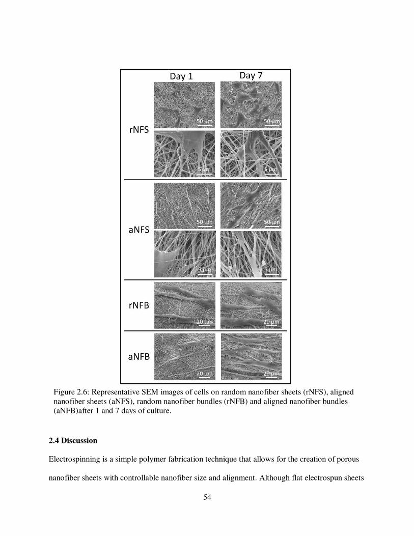
54

2.4 Discussion

Electrospinning is a simple polymer fabrication technique that allows for the creation of porous

nanofiber sheets with controllable nanofiber size and alignment. Although flat electrospun sheets

Figure 2.6: Representative SEM images of cells on random nanofiber sheets (rNFS), aligned nanofiber sheets (aNFS), random nanofiber bundles (rNFB) and aligned nanofiber bundles (aNFB)after 1 and 7 days of culture.

55

are suitable for cell growth, inherent limitations impede their use in tendon and ligament

regeneration. It is challenging to produce flat sheets of electrospinning that are more than 1mm

thick due to electrostatic repulsion properties that prevent excessive fiber deposition 40. Although

some research groups have attempted to laminate flat sheets of electrospinning and incorporate

hydrogels to create more robust scaffolds, the mechanical properties are still relatively low 31,41–

44. In order to make electrospun scaffolds more applicable for large-scale tissue engineering

purposes, it is necessary to modify the geometry of flat sheets to better mimic the structure and

mechanical properties of target tissues, in this case, tendons and ligaments, both load bearing

orthopedic connective tissues.

In the present study, we have investigated how to vary the structure of nanofiber sheets by

modifying both the geometry and nanofiber orientation in order to better replicate the form and

function of tendons and ligaments and improve mechanical properties. We present a novel

technique for improving the mechanical properties of nanofiber scaffolds while maintaining the

complex underlying fiber architecture. The electrospinning process was conducted using a

rotating mandrel, which allowed for modulation of the nanofiber orientation. The parallel

alignment of PCL nanofibers in aligned nanofiber sheets closely mimicked the size scale and

structure of collagen fibers within the ACL 45,46. Although the aligned nanofibers mimic the

orientation of collagen fibers in the native ACL, the pores between the nanofibers are much

larger than the spaces between the densely packed ACL collagen fibers. These larger pores in the

electrospun scaffold are necessary for encouraging cell infiltration and production of

extracellular matrix. In addition to modifying the orientation of electrospun nanofibers, this study

reports a method for modifying flat nanofiber sheets into a three-dimensional bundle of

56

nanofibers. The size of the nanofiber bundles (400-500 µm) mimics the size of collagen fascicles

(50-500 µm) found in load-bearing orthopedic tissues 4,45. Modifying the geometry of

electrospun sheets to create nanofiber bundles results in a novel cylindrical scaffold that is

remarkably robust, suggesting that it may be more feasible for clinical use. By fabricating

nanofiber bundles from random or aligned nanofiber sheets we were able to modulate the

mechanical properties as well as the cellular response.

In order for a tissue-engineered scaffold to provide a suitable replacement for native human

tendons and ligaments, it is desirable for the scaffold to possess mechanical properties that are

similar to native ACL. An important consideration in the calculation of material properties is

how sample cross-sectional area is determined. Since electrospun sheets are highly porous,

simply utilizing the width and the “as-spun” thickness of the nanofiber sheet to calculate the

cross-sectional area overestimates the amount of material that is actually present and

consequently underestimates the mechanical properties. To overcome this problem, in addition to

calculating the as-spun cross-sectional area of nanofiber sheets and bundles, we compressed

nanofiber sheets and bundles to eliminate pore space and used additional SEM images to

determine true material area. In this way, it is possible to determine both the apparent properties

of the bulk scaffold, as well as the inherent properties of the electrospun material. A limitation to

this method was the difficulty in verifying if all pore space had been completely eliminated using

only visual inspection of SEM images; however this work is still the first to calculate the

mechanical properties of electrospun scaffolds by taking into account the true material cross-

sectional area.

57

Firstly, altering nanofiber orientation so nanofiber sheets consisted of primarily aligned

nanofibers increased the elastic modulus by ~125% and the yield stress by ~150%. These

differences in mechanical properties are possibly due to more fibers being present in parallel

over which to distribute the applied loads, thus requiring more force to cause elastic deformation.

Previous studies of the mechanical behavior of aligned nanofiber sheets of electrospun PCL have

reported the elastic modulus to range from 20-40 MPa and the yield stress to range from 2-4

MPa 23,24,47,48. Despite some expected variation due to spinning technique and duration, these

previously reported values are relatively similar to values calculated in this study utilizing the as-

spun cross-sectional area but are up to an order of magnitude lower than the values calculated

utilizing the compressed cross-sectional area. Similar to our findings, previous studies assessing

the moduli of nanofiber sheets have shown aligned nanofiber sheets to have moduli 75-140%

higher than the random nanofiber sheets (23,47,48).

In addition to altering nanofiber orientation, altering the geometry of nanofiber sheets

significantly affected the mechanical properties. When random nanofiber sheets were used to

create randomly oriented nanofiber bundles there was no significant difference in elastic

modulus, however, the elastic modulus of aligned nanofiber bundles was observed to be ~55%

lower than the elastic modulus of aligned nanofiber sheets. The decrease in elastic modulus of

aligned nanofiber bundles may be due to the extent of nanofibers that were engaged during the

tensile test and bearing the applied load. However, it is difficult to speculate exactly why

scaffolds with similar nanofiber alignment but different geometries possess different material

properties. We hypothesize that these differing material properties may be due to interactions

between the fiber layers and varying recruitment of the nanofibers to bear the applied loads.

58

Based on the low standard errors of the measured material properties, we feel confident that

sample preparation and testing techniques are not responsible for the differing properties. Further

experiments will be necessary to elucidate the exact reasons for the variation in material

properties with altered scaffold geometry.

One limitation of the mechanical testing techniques used in this study, which could limit the

interpretation of the results was the different techniques used to measure the strain of flat sheets

and nanofiber bundles. Speckle tracking of India ink dots was used to measure strain in the

central region of the dog-bone shaped flat sheets, however, due to the small size of the nanofiber

bundles (~0.5 mm) and limited resolution of the camera used to track the samples the speckle

coating technique could not be used. Instead, strain for nanofiber bundles was measured using

grip-to-grip displacement from the servo-hydraulic mechanical test system (Bionic Model 370.02

MTS Systems Corporation, Eden Prairie, MN).

Previous studies have assessed the effects of modifying the geometry of electrospun scaffolds.

Computational work conducted by Nerurkar et al. found that any modulus reinforcement effects

from stacking layers of electrospun fibers only occurred when layers were oriented in opposing

directions and fibers were forced to undergo rotation under tensile loading to align along the axis

of the load, generating additional shear forces 49. Similarly, Fisher et al., reported that when

assessing the mechanical properties of stacks of sheets of electrospinning, only layers with “non-

orthogonal” orientations showed evidence for a mechanical reinforcement effect compared to

individual sheets 41. Previous groups investigating the effects of twisting or braiding electrospun

nanofibers have observed trends of increasing elastic modulus with more complex geometry,

59

however, this could be attributed to variation in the calculation of scaffold cross-sectional area

29,30,50. Nerurkar et al. showed that layers of electrospun fibers stiffened after extended cell

culture, likely due to cell matrix deposition between layers, which suggests that aligned

nanofiber bundles may develop a higher elastic modulus over time in culture 51.

Modifying geometry also resulted in significant differences in yield stress and strain of the

resultant scaffolds, particularly when nanofibers were aligned. Aligned nanofiber bundles had an

average yield stress 90% higher than aligned nanofiber sheets and an average yield strain 130%

higher than aligned nanofiber sheets. This is promising for the proposed ligament tissue

engineering applications because although ligaments typically only undergo less than 10% strain

during normal loading, it would be valuable for scaffolds to be able to sustain higher stresses and

strains prior to plastic deformation 36. Overall, modifying both geometry and nanofiber

orientation to create a nanofiber bundle composed of aligned nanofibers resulted in a scaffold

with modulus and yield stress and strain values within the range of the native human ACL (Table

2-1). Previous research has also assessed the mechanical properties of the sub-structures of the

native human ACL, including the anteromedial, anterolateral, and posterior bundles as well as

individual fascicles 52,53. The anteromedial and anterolateral bundle and individual fascicles have

moduli that are higher than that of the entire ACL and higher than that of aligned nanofiber

bundles. This presents a limitation of the described scaffold since it does not precisely match the

material properties of the structures that compose the native human ACL. However, the modulus

of aligned nanofiber bundles does closely match the modulus of the posterolateral bundle.

Additionally, the yield stress and yield strain of aligned nanofiber bundles are within in the range

of the tensile strength and yield strain of ACL bundles as well as ACL fascicles. In the context of

60

ACL replacement scaffolds, yield stress, and strain are comparable to tensile strength and failure

strain since a scaffold that has plastically deformed has essentially “failed” as it is no longer able

to properly fulfill the role of the ACL. Notably, the results of the present study suggest that

aligned nanofiber bundles may be suitable for use as a tissue-engineered scaffold, since the

modulus and the yield properties of the scaffold meet the mechanical demands of the native

ACL, and potentially other tendons and ligaments as well. Additional modification, such as

combining multiple nanofiber bundles into a single construct may further alter scaffold

mechanical properties. Preliminary work has suggested that securing together the ends of ~100

nanofiber bundles using solvent cast solid PCL produces a structure with significantly higher

stiffness and failure load.

Modulus (MPa) Yield Stress (MPa) Yield Strain

Aligned nanofiber bundle 154 ± 28 54 ± 12 0.38 ± 0.03

Modulus (MPa) Tensile Strength

(MPa)

Failure

Strain

Noyes & Grood 54 ACL, Old 65 ± 24 13 ± 5 0.49 ± 0.12

ACL, Young 111 ± 26 38 ± 9 0.60 ± 0.07

Chandrashekar 55 ACL, Male 128 ± 35 26 ± 10 0.30 ± 0.06

ACL, Female 99 ± 50 23 ± 9 0.27 ± 0.08

Butler 52 ACL fascicle 345 ± 22 36 ± 3 0.15 ±0.008

Butler 53 ACL

anteromedial bundle

283 ± 114 46 ± 20 0.19 ± 0.03

ACL anterolateral

bundle

285.9 ± 141 31 ± 11 0.16 ± 0.04

ACL posterolateral

bundle

154 ± 119.5 15 ± 10 0.15 ± 0.05

Table 2.1: Material properties of aligned nanofiber bundles compared to properties of human ACL from previous studies.

61

All nanofiber sheets and bundles were able to support cell adhesion and proliferation, which was

expected since electrospun PCL nanofibers have previously been shown to support a variety of

cell types 27,56,57. However, quantitative measures indicated that there were some differences in

both cell viability and cell morphology between nanofiber sheets and bundles. Higher

fluorescence from CellTiter-Blue viability assays on nanofiber bundles may be due to the larger

surface area of nanofiber bundles compared to nanofiber sheets. The results of cell counts based

on DAPI stained nuclei indicated no differences in cell number on any nanofiber sheets and

bundles at the Day 1 or Day 7 time points. Any discrepancies between CellTiter-Blue viability

assay results and cell count results may be because cells proliferated around the curved edges of

the nanofiber bundles or migrated into the center of the nanofibers where they could not be

imaged. The quantification of cell shape showed interesting effects of both geometry and

nanofiber orientation on cell morphology. Similar to reports from other groups, after 7 days in

culture cells on aligned nanofiber sheets were significantly more elongated along the primary

nanofiber direction compared to cells on random sheets 23,27,58. However, on nanofiber bundles,

cells were more elongated compared to nanofiber sheets regardless of fiber alignment. It is

hypothesized that the cells may have detected the convex curvature of the cylindrical nanofiber

bundles, regardless of fiber alignment, and consequently aligned along the length of the

nanofiber bundle. This novel finding suggests that the micro-scale geometry of nanofiber

bundles has a separate and significant impact on cell morphology. It has also been previously

shown that substrate stiffness has important effects on cell development and differentiation 59,60.

Specifically, the modulus of the substrate influences cytoskeleton assembly and; on less stiff

surfaces cells have reduced spreading and increased rates of motility 61. Additionally,

mesenchymal stem cells differentiation response has been shown to be acutely sensitive to the

62

elasticity of the underlying substrate 62. Because the scaffolds in this study demonstrate

significantly different levels of stiffness and this may play a role in altering cell morphology. The

ability to modulate cell morphology is important for tissue engineering applications because cell

shape affects numerous cell processes, including cell migration and communication as well as

cellular differentiation 63. A limitation of the current nanofiber sheets and bundles is the low

porosity (pore sizes of approximately 5 µm), which could potentially limit cell infiltration into

the interior of the scaffolds. Cell infiltration could be encouraged by modifying the

electrospinning technique to include sacrificial fibers/porogens or increasing the nanofiber

diameter in order to increase overall porosity 64–66.

2.5 Conclusions

This work presents a novel cylindrical electrospun scaffold with robust mechanical properties

and a complex underlying nanofiber structure. Nanofiber orientation and geometry of

electrospun PCL were modified to mimic the fascicles of native tendon and ligament. Aligned

nanofiber bundles had the highest yield stresses and strains, while still maintaining a relatively

high elastic modulus. Remarkably, these mechanical properties are within the range of the native

human ACL. For the first time in this work, the mechanical properties of electrospun scaffolds

were calculated using a true material cross-sectional area, with pore space between nanofibers

eliminated to prevent an underestimation of properties. Additionally all nanofiber sheets and

bundles were able to support cell adhesion and proliferation for up to 7 days in culture; however,

nanofiber bundles are preferable for encouraging the parallel elongation of adipose-derived stem

cells. The mechanical properties and cell response of aligned electrospun nanofiber bundles

suggest they are a promising scaffold for orthopedic tissue engineering applications. Future

63

studies will investigate the utilization of growth factors to promote cell differentiation into a

ligamentous phenotype and the effect of combining multiple nanofiber bundles into a more

complex scaffold to further alter mechanical properties.

64

REFERENCES

1. Giugliano, D. N. & Solomon, J. L. ACL Tears in Female Athletes. Phys. Med. Rehabil.

Clin. N. Am. 18, 417–438 (2007).

2. Prodromos, C. C., Han, Y., Rogowski, J., Joyce, B. & Shi, K. A Meta-analysis of the Incidence of Anterior Cruciate Ligament Tears as a Function of Gender, Sport, and a Knee Injury-Reduction Regimen. Arthrosc. J. Arthrosc. Relat. Surg. 23, 1320–1325 (2007).

3. Clayton, R. A. E. & Court-Brown, C. M. The epidemiology of musculoskeletal tendinous and ligamentous injuries. Injury 39, 1338–1344 (2008).

4. Kastelic, J., Galeski, A. & Baer, E. The multicomposite structure of tendon. Connect.

Tissue Res. 6, 11–23 (1978).

5. Arnoczky, S. Anatomy of the anterior cruciate ligament. Clin. Orthop. Relat. Res. 172, 19–25 (1983).

6. Buss, D. D., Warren, R. F., Wickiewicz, T. L., Galinat, B. J. & Panariello, R. Arthroscopically assisted reconstruction of the anterior cruciate ligament with use of autogenous patellar-ligament grafts. Results after twenty-four to forty-two months. J.

Bone Joint Surg. Am. 75, 1346–1355 (1993).

7. Langan, P. & Fontanetta, A. P. Rupture of the patellar tendon after use of its central third. Orthop. Rev. 16, 317–321 (1987).

8. Simonds, R. J., Holmberg, S. D., Hurwitz, R. L., Coleman, T. R., Bottenfield, S., Conley, L. J., Kohlenberg, S. H., Castro, K. G., Dahan, B. A. & Schable, C. A. Transmission of human immunodeficiency virus type 1 from a seronegative organ and tissue donor. N.

Engl. J. Med. 326, 726–732 (1992).

9. Dillon, C. F., Rasch, E. K., Gu, Q. & Hirsch, R. Prevalence of knee osteoarthritis in the United States: arthritis data from the Third National Health and Nutrition Examination Survey 1991-94. J. Rheumatol. 33, 2271–9 (2006).

10. Guccione, A. A., Felson, D. T., Anderson, J. J., Anthony, J. M., Zhang, Y., Wilson, P. W., Kelly-Hayes, M., Wolf, P. A., Kreger, B. E. & Kannel, W. B. The effects of specific medical conditions on the functional limitations of elders in the Framingham Study. Am. J.

Public Health 84, 351–8 (1994).

11. Leong, N. L., Petrigliano, F. A. & McAllister, D. R. Current tissue engineering strategies in anterior cruciate ligament reconstruction. J. Biomed. Mater. Res. A 102, 1614–24 (2014).

65

12. Petrigliano, F. A., McAllister, D. R. & Wu, B. M. Tissue engineering for anterior cruciate ligament reconstruction: a review of current strategies. Arthroscopy 22, 441–451 (2006).

13. Dunn, M. G., Liesch, J. B., Tiku, M. L. & Zawadsky, J. P. Development of fibroblast-seeded ligament analogs for ACL reconstruction. J. Biomed. Mater. Res. 29, 1363–1371 (1995).

14. Bellincampi, L. D., Closkey, R. F., Prasad, R., Zawadsky, J. P. & Dunn, M. G. Viability of fibroblast-seeded ligament analogs after autogenous implantation. J. Orthop. Res. 16, 414–420 (1998).

15. Chen, J., Altman, G. H., Karageorgiou, V., Horan, R., Collette, A., Volloch, V., Colabro, T. & Kaplan, D. L. Human bone marrow stromal cell and ligament fibroblast responses on RGD-modified silk fibers. J. Biomed. Mater. Res. A 67, 559–570 (2003).

16. Altman, G. H., Horan, R. L., Lu, H. H., Moreau, J., Martin, I., Richmond, J. C. & Kaplan, D. L. Silk matrix for tissue engineered anterior cruciate ligaments. Biomaterials 23, 4131–41 (2002).

17. Danylchuk, K. D., Finlay, J. B. & Krcek, J. P. Microstructural organization of human and bovine cruciate ligaments. Clin. Orthop. Relat. Res. 131, 294–298 (1978).

18. Butler, D. L., Goldstein, S. a & Guilak, F. Functional tissue engineering: the role of biomechanics. J. Biomech. Eng. 122, 570–5 (2000).

19. Vunjak-Novakovic, G., Altman, G., Horan, R. & Kaplan, D. L. Tissue engineering of ligaments. Annu. Rev. Biomed. Eng. 6, 131–56 (2004).

20. Pedicini, A. & Farris, R. J. Mechanical behavior of electrospun polyurethane. Polymer. 44, 6857–6862 (2003).

21. Li, D. & Xia, Y. Electrospinning of Nanofibers: Reinventing the Wheel? Adv. Mater. 16, 1151–1170 (2004).

22. Pham, Q. P., Sharma, U. & Mikos, A. G. Electrospinning of polymeric nanofibers for tissue engineering applications: a review. Tissue Eng. 12, 1197–211 (2006).

23. Li, W. J., Mauck, R. L., Cooper, J. a, Yuan, X. & Tuan, R. S. Engineering controllable anisotropy in electrospun biodegradable nanofibrous scaffolds for musculoskeletal tissue engineering. J. Biomech. 40, 1686–93 (2007).

24. Choi, J. S., Lee, S. J., Christ, G. J., Atala, A. & Yoo, J. J. The influence of electrospun aligned poly(e-caprolactone)/collagen nanofiber meshes on the formation of self-aligned skeletal muscle myotubes. Biomaterials 29, 2899–2906 (2008).

66

25. Balguid, A., Mol, A., Van Marion, M. H., Bank, R. A., Bouten, C. V. C. & Baaijens, F. P. T. Tailoring fiber diameter in electrospun poly(epsilon-caprolactone) scaffolds for optimal cellular infiltration in cardiovascular tissue engineering. Tissue Eng. Part A 15, 437–44 (2009).

26. Baker, B. M., Gee, A. O., Metter, R. B., Nathan, A. S., Marklein, R. a, Burdick, J. a & Mauck, R. L. The potential to improve cell infiltration in composite fiber-aligned electrospun scaffolds by the selective removal of sacrificial fibers. Biomaterials 29, 2348–58 (2008).

27. Baker, B. M. & Mauck, R. L. The effect of nanofiber alignment on the maturation of engineered meniscus constructs. Biomaterials 28, 1967–77 (2007).

28. Ayres, C., Bowlin, G. L., Henderson, S. C., Taylor, L., Shultz, J., Alexander, J., Telemeco, T. A. & Simpson, D. G. Modulation of anisotropy in electrospun tissue-engineering scaffolds: Analysis of fiber alignment by the fast Fourier transform. Biomaterials 27, 5524–34 (2006).

29. Barber, J. G., Handorf, A. M., Allee, T. J. & Li, W.-J. Braided nanofibrous scaffold for tendon and ligament tissue engineering. Tissue Eng. Part A 19, 1265–74 (2013).

30. Freeman, J. W., Woods, M. D. & Laurencin, C. T. Tissue engineering of the anterior cruciate ligament using a braid-twist scaffold design. J. Biomech. 40, 2029–36 (2007).

31. Petrigliano, F. A., Arom, G. A., Nazemi, A. N., Yeranosian, M. G., Wu, B. M. & McAllister, D. R. In Vivo Evaluation of Electrospun Polycaprolactone Graft for Anterior Cruciate Ligament Engineering. Tissue Eng. Part A 21, 1228–2136 (2015).

32. Lee, C. H., Shin, H. J., Cho, I. H., Kang, Y.-M., Kim, I. A., Park, K.-D. & Shin, J.-W. Nanofiber alignment and direction of mechanical strain affect the ECM production of human ACL fibroblast. Biomaterials 26, 1261–70 (2005).

33. Berens, P. CircStat: A MATLAB toolbox for circular statistics. J. Stat. Softw. 31, 1–21 (2009).

34. Noyes, F. R., DeLucas, J. L. & Torvik, P. J. Biomechanics of anterior cruciate ligament failure: an analysis of strain-rate sensitivity and mechanisms of failure in primates. J.

Bone Joint Surg. Am. 56, 236–53 (1974).

35. Fleming, B. C., Beynnon, B. D., Renstrom, P. a, Johnson, R. J., Nichols, C. E., Peura, G. D. & Uh, B. S. The strain behavior of the anterior cruciate ligament during stair climbing: an in vivo study. Arthroscopy 15, 185–91 (1999).

36. Withrow, T. J., Huston, L. J., Wojtys, E. M. & Ashton-Miller, J. a. The effect of an impulsive knee valgus moment on in vitro relative ACL strain during a simulated jump landing. Clin. Biomech. 21, 977–83 (2006).

67

37. Jones, E. M. C., Silberstein, M. N., White, S. R. & Sottos, N. R. In Situ Measurements of Strains in Composite Battery Electrodes during Electrochemical Cycling. Exp. Mech. 54, 971–985 (2014).

38. Leszczak, V., Baskett, D. & Popat, K. Smooth Muscle Cell Functionality on Collagen Immobilized Polycaprolactone Nanowire Surfaces. J. Funct. Biomater. 5, 58–77 (2014).

39. Trujillo, N. A. & Popat, K. C. Osteogenic Differentiation of Adipose Derived Stem Cells on Polycaprolactone Nanowire Surfaces. J. Biomater. Tissue Eng. 3, 542–553 (2013).

40. Tzezana, R., Zussman, E. & Levenberg, S. A layered ultra-porous scaffold for tissue engineering, created via a hydrospinning method. Tissue Eng. Part C. Methods 14, 281–288 (2008).

41. Fisher, M. B., Henning, E. a., Söegaard, N., Bostrom, M., Esterhai, J. L. & Mauck, R. L. Engineering meniscus structure and function via multi-layered mesenchymal stem cell-seeded nanofibrous Scaffolds. J. Biomech. (2015).

42. Leong, N. L., Kabir, N., Arshi, A., Nazemi, A., Wu, B., Petrigliano, F. A. & McAllister, D. R. Evaluation of polycaprolactone scaffold with basic fibroblast growth factor and fibroblasts in an athymic rat model for anterior cruciate ligament reconstruction. Tissue

Eng. Part A 21, 1859–68 (2015).

43. Strange, D. G. T., Tonsomboon, K. & Oyen, M. L. Mechanical behaviour of electrospun fibre-reinforced hydrogels. J. Mater. Sci. Mater. Med. 25, 681–90 (2014).

44. Baek, J., Chen, X., Sovani, S., Jin, S., Grogan, S. P. & D’Lima, D. D. Meniscus tissue engineering using a novel combination of electrospun scaffolds and human meniscus cells embedded within an extracellular matrix hydrogel. J. Orthop. Res. 572–583 (2015).

45. Duthon, V. B., Barea, C., Abrassart, S., Fasel, J. H., Fritschy, D. & Ménétrey, J. Anatomy of the anterior cruciate ligament. Knee Surg. Sports Traumatol. Arthrosc. 14, 204–13 (2006).

46. Yahia, L. H. & Drouin, G. Microscopical investigation of canine anterior cruciate ligament and patellar tendon: collagen fascicle morphology and architecture. J. Orthop.

Res. 7, 243–51 (1989).

47. Kim, G. H. Electrospun PCL nanofibers with anisotropic mechanical properties as a biomedical scaffold. Biomed. Mater. 3, 1–8 (2008).

48. Thomas, V., Jose, M. V, Chowdhury, S., Sullivan, J. F., Dean, D. R. & Vohra, Y. K. Mechano-morphological studies of aligned nanofibrous scaffolds of polycaprolactone fabricated by electrospinning. J. Biomater. Sci. Polym. Ed. 17, 969–84 (2006).

68

49. Nerurkar, N. L., Sen, S., Baker, B. M., Elliott, D. M. & Mauck, R. L. Dynamic culture enhances stem cell infiltration and modulates extracellular matrix production on aligned electrospun nanofibrous scaffolds. Acta Biomater. 7, 485–91 (2011).

50. Bosworth, L. A., Alam, N., Wong, J. K. & Downes, S. Investigation of 2D and 3D electrospun scaffolds intended for tendon repair. J. Mater. Sci. Mater. Med. 24, 1605–14 (2013).

51. Nerurkar, N. L., Baker, B. M., Sen, S., Wible, E. E., Elliott, D. M. & Mauck, R. L. Nanofibrous biologic laminates replicate the form and function of the annulus fibrosus. Nat. Mater. 8, 986–992 (2009).

52. Butler, D. L., Kay, M. D. & Stouffer, D. C. Comparison of material properties in fascicle-bone units from human patellar tendon and knee ligaments. J. Biomech. 19, 425–32 (1986).

53. Butler, D. L., Guan, Y., Kay, M. D., Cummings, J. F., Feder, S. M. & Levy, M. S. Location-dependent variations in the material properties of the anterior cruciate ligament. J. Biomech. 25, 511–518 (1992).

54. Noyes, F. R. & Grood, E. S. The strength of the anterior cruciate ligament in humans and Rhesus monkeys. J. Bone Joint Surg. Am. 58, 1074–82 (1976).

55. Chandrashekar, N., Mansouri, H., Slauterbeck, J. & Hashemi, J. Sex-based differences in the tensile properties of the human anterior cruciate ligament. J. Biomech. 39, 2943–50 (2006).

56. Ruckh, T. T., Kumar, K., Kipper, M. J. & Popat, K. C. Osteogenic differentiation of bone marrow stromal cells on poly(epsilon-caprolactone) nanofiber scaffolds. Acta Biomater. 6, 2949–59 (2010).

57. Nerurkar, N. L., Elliott, D. M. & Mauck, R. L. Mechanics of oriented electrospun nanofibrous scaffolds for annulus fibrosus tissue engineering. J. Orthop. Res. 25, 1018–28 (2007).

58. Ghasemi-Mobarakeh, L., Prabhakaran, M. P., Morshed, M., Nasr-Esfahani, M.-H. & Ramakrishna, S. Electrospun poly(epsilon-caprolactone)/gelatin nanofibrous scaffolds for nerve tissue engineering. Biomaterials 29, 4532–9 (2008).

59. Pelham, R. J. & Wang, Y. L. Cell locomotion and focal adhesions are regulated by the mechanical properties of the substrate. in Biol. Bull. 194, 348–350 (1998).

60. Yeung, T., Georges, P. C., Flanagan, L. a., Marg, B., Ortiz, M., Funaki, M., Zahir, N., Ming, W., Weaver, V. & Janmey, P. a. Effects of substrate stiffness on cell morphology, cytoskeletal structure, and adhesion. Cell Motil. Cytoskeleton 60, 24–34 (2005).

69

61. Discher, D. E., Janmey, P. & Wang, Y.-L. Tissue cells feel and respond to the stiffness of their substrate. Science 310, 1139–43 (2005).

62. Engler, A. J., Sen, S., Sweeney, H. L. & Discher, D. E. Matrix Elasticity Directs Stem Cell Lineage Specification. Cell 126, 677–689 (2006).

63. Kilian, K. A., Bugarija, B., Lahn, B. T. & Mrksich, M. Geometric cues for directing the differentiation of mesenchymal stem cells. Proc. Natl. Acad. Sci. U. S. A. 107, 4872–4877 (2010).

64. Baker, B. M., Shah, R. P., Silverstein, A. M., Esterhai, J. L., Burdick, J. a & Mauck, R. L. Sacrificial nanofibrous composites provide instruction without impediment and enable functional tissue formation. Proc. Natl. Acad. Sci. U. S. A. 109, 14176–81 (2012).

65. Nam, J., Huang, Y., Agarwal, S. & Lannutti, J. Improved cellular infiltration in electrospun fiber via engineered porosity. Tissue Eng. 13, 2249–57 (2007).

66. Wang, K., Zhu, M., Li, T., Zheng, W., Xu, L. L., Zhao, Q., Kong, D. & Wang, L. Improvement of Cell Infiltration in Electrospun Polycaprolactone Scaffolds for the Construction of Vascular Grafts. J. Biomed. Nanotechnol. 10, 1588–1598 (2014).

70

CHAPTER 3:

HIERARCHICALLY STRUCTURED ELECTROSPUN SCAFFOLDS WITH

CHEMICALLY CONJUGATED GROWTH FACTOR FOR LIGAMENT TISSUE

ENGINEERING2

3.1 Introduction

The anterior cruciate ligament (ACL) is located in the knee and runs from the lateral posterior

aspect of the femoral condyle to the medial anterior aspect of the tibial plateau1. The ACL is vital

for joint stability and it functions primarily as a restraint to excessive translations of the tibia

relative to the femur 2,3. The ACL is primarily composed of collagen fibers arranged in a unique

hierarchical structure and a lack of vascularization means that the ligament has a low intrinsic

healing capacity4,5. It is estimated that up to 200,000 ACL injuries occur in the United States

annually and the monetary burden of these injuries and subsequent treatment is estimated to be

$1 billion each year6,7. Untreated tears of the ACL can cause knee pain, bone bruising, excessive

joint laxity, and damage to the surrounding cartilage and menisci of the knee. Following an ACL

injury, surgical replacement of the ACL with an autograft or allograft is typically attempted to

restore function and stability to the injured knee. However, drawbacks exist to both intervention

techniques. Although allografts have been historically successful, morbidity at the site of tissue

donation can result in pain, tendonitis, and weakness8,9. Allograft tissue obtained from cadavers

can also be used to replace the ACL however tissue supply is limited and disease transmission

can be problematic10. Thus there is interest in developing a tissue-engineered replacement ACL

that can overcome the limitations of traditional allografts and autografts.

2 This chapter has been published as a Research Paper in Tissue Engineering Part A (23, 2017). All content has been adapted with permission from Mary Ann Liebert, Inc.

71

The field of tissue engineering aims to combine scaffolds, cells, and signaling molecules to

create a replacement for damaged biological tissue. Electrospinning is a versatile scaffold

fabrication technique which uses biodegradable polymers to create a nanoscale structure that

mimics the structure of the extracellular matrix11,12. Braided electrospun scaffolds have been

shown to encourage cell proliferation and upregulation of tenogenic markers13,14 whereas

laminated electrospun sheets have successfully encouraged cell infiltration15. However, both of

these approaches have demonstrated inferior mechanical properties12-14. A tissue engineered

ACL that matches the hierarchical structure of the native ligament, has sufficient mechanical

properties and encourages the production of ligamentous tissue deposition in vitro and in vivo

will likely improve the clinical treatment of ACL injury.

Our group has previously developed a technique for modifying flat sheets of aligned electrospun

polycaprolactone (PCL) nanofibers to create a more robust structure16. These cylindrical

“nanofiber bundles” are approximately 500 µm in diameter and are composed of nanofibers

aligned along the longitudinal axis that mimic the native ACL structure. Nanofiber bundles are

able to support short-term cell growth and elongated cell morphology and have material

properties that are comparable to that of the native human ACL16–18. The smallest functional

units of the ACL are collagen fibrils that range in size from 50-500 nm and are primarily

oriented parallel to the longitudinal axis19,20. The individual PCL nanofibers that compose the

electrospun sheets used in this study mimic this size scale16. Collagen fibrils of the ACL are

organized into fibers and numerous collagen fibers are grouped into fascicles, approximately

100-500 µm in size. The size of these collagen fascicles is similar to the size of one nanofiber

bundles. In the native ACL, multiple collagen fascicles are grouped together to form the entire

72

ligament. Thus, in an effort to mimic the hierarchical ACL structure, multiple nanofiber bundles

were combined together to form a 3D scaffold for this study.

Growth factors are chemical signaling molecules that can be used to direct cell behavior. In the

context of ligament tissue engineering, it would be beneficial to utilize a growth factor that

encourages cell proliferation as well as the deposition of extracellular matrix material

characteristic of native ligaments21. Connective tissue growth factor (CTGF) is a 36-38 kDa

heparin-binding protein characterized by multiple conserved cysteine-rich domains22. CTGF is

involved in a variety of physiological processes including angiogenesis, embryo development,

and would healing23. CTGF has been previously shown to encourage fibroblastic differentiation

of stem cells, as evidenced by cell proliferation, gene expression changes, and increased matrix

deposition22,24. The most common way to expose cells to growth factors is by introducing the

growth factor to the cells in vitro in the cell growth media. The major drawback to this technique

is that growth factors have a relatively short half-life in cell growth media and are rapidly

inactivated, thus making it necessary to introduce fresh growth factor during each media

change25. Additionally, sustained growth factor delivery in an in vivo setting is a challenge that

needs to be addressed to facilitate the development of functionalized scaffolds. One strategy to

address these challenges is to conjugate growth factors to the scaffold surface using a covalent

chemical conjugation procedure26. This surface modification-technique utilizes chemical bonds

to immobilize the growth factors to exposed functional groups on a scaffold. Chemical

conjugation of growth factors to a scaffold creates functionalized nanofiber scaffolds with

tunable growth factor release and a prolonged influence on cell behavior25,26. Previously,

73

electrospun scaffolds with chemically conjugated growth factors have been used to encourage

neuronal differentiation, enhance wound healing, and stimulate osteogenic cellular activity27–29.

Previously, we have shown that individual PCL nanofiber bundles support short-term in vitro

cell growth and proliferation16, hence, this study is aimed at assessing long-term cell behavior

on a 3D scaffold with multiple nanofiber bundles and chemically conjugated CTGF, both in vitro

and in vivo. It is hypothesized that the combination of the unique hierarchical structure and the

presence of CTGF will induce the deposition of tissue that is characteristic of ligaments,

primarily collagen type I and type III.

3.2 Methods

3.2.1 Scaffold fabrication

Flat sheets of aligned nanofibers were fabricated using an electrospinning technique as detailed

previously16. A 10% w/v solution of polycaprolactone (PCL, Mw = 80,000, Sigma 440744, St.

Louis, MO) was prepared in a 3:1 v/v mixture of chloroform and methanol. The electrospinning

solution was ejected horizontally from a glass syringe outfitted with an 18-gauge blunt tipped

needle at a rate of 2 mL/hr for 15 min. To create sheets of aligned nanofibers (Figure 3.1A), the

collector surface was a rotating aluminum drum located 10 cm from the needle tip and rotating

with a linear velocity of approximately 12 m/s. These sheets were further used to create

cylindrical bundles of nanofibers (Figure 3.1B) by excising a rectangular portion of the sheet

(approximately 5 cm x 175 cm) and rolling it up tightly into a cylinder16. This resulted in

nanofiber bundles that were approximately 0.5 mm in diameter and 175 mm length, with

74

nanofibers aligned along the longitudinal axis. For further studies, nanofiber bundles were cut to

20 mm in length

3.2.2 Growth factor conjugation

CTGF (Sigma SRP4702, St. Louis, MO) was covalently bound to nanofiber bundles (n=3) using

a multi-step chemical conjugation technique (Figure 3.2A). First amines were added by

incubating nanofiber bundles in a 5% v/v aqueous solution of polyallylamine (Sigma 479136, St.

Louis, MO) with simultaneous ultraviolet radiation for 25 min. Next nanofiber bundles were

incubated on a shaker plate in a solution 10% w/w solution of N-succinimidyl-3-

Figure 3.1: Aligned nanofibers (A), nanofiber bundle (B), scaffold composed of ~20 nanofiber bundles (C), and small scaffold composed of 4 nanofiber bundles (D).

75

maleimidoproprionate (TCI America SO427, Portland, OR) N,N-dimethylformamide (Sigma

227056, St. Louis, MO) for 1 hr to add on maleimide terminals. In the final step, the nanofiber

bundles were incubated in a 50 ng/mL solution of CTGF for 2 hr. Between subsequent steps, the

nanofiber bundles were rinsed in triplicate using deionized water (dH2O), incubated in distilled

dH2O for 2 hr, and then rinsed an additional 3 times in dH2O to ensure all excess chemicals had

been leached from the nanofibers.

Figure 3.2: Chemical conjugation procedure (A), XPS survey spectra showing increasing nitrogen peak (B), immunofluorescence staining of conjugated CTGF (C), amount of CTGF conjugated (D), and CTGF release over a 14 day period (E).

76

CTGF conjugation efficiency was assessed using X-ray photoelectron spectroscopy (XPS, PE-

5800, Physical Electronics, Chanhassen, MN). XPS was conducted after each subsequent

modification step to assess the surface composition of nitrogen, which is indicative of successful

conjugation of each linker component as well as CTGF. Survey spectra were collected from 0 to

1100eV with a pass energy of 187.85 and data for the percent elemental composition were

calculated using the instrument specific software (PHI MultiPak, Physical Electronics,

Chanhassen, MN).

Distribution of CTGF was assessed using immunofluorescence labeling. To

immunofluorescently label the conjugated CTGF, nanofiber bundles were first rinsed with

phosphate-buffered saline (PBS) and then incubated with 10% donkey serum (Santa Cruz

Biotechnology sc-2044, Santa Cruz, CA) in PBS for 20 min. After rinsing again in PBS,

nanofiber bundles were incubated in the primary antibody against CTGF (goat, Santa Cruz

Biotechnology sc-14939, Santa Cruz, CA) prepared in 1.5% donkey serum at a concentration of

4 µg/mL in PBS for 1 hr. Nanofiber bundles were then rinsed in PBS in triplicate for 5 min each.

Next, nanofiber bundles were incubated in the secondary antibody labeled with fluorescein

isothiocyanate (FITC, donkey anti-goat, Santa Cruz Biotechnology sc-2024, Santa Cruz, CA)

prepared in 1.5% donkey serum at a concentration of 4 µg/mL in PBS for 1 hr. Nanofiber

bundles were rinsed again in PBS prior to imaging with a fluorescent microscope (Olympus

IX70, Center Valley, PA).

An enzyme-linked immunosorbent assay (ELISA, PeproTech 900-m317, Rocky Hill, NJ) was

used to characterize the amount of CTGF initially conjugated to each nanofiber bundle as well as

77

the cumulative release of CTGF from nanofiber bundles over a 2 week time period. After the

final conjugation step, the CTGF solution was used to measure the amount of growth factor that

remained unconjugated. Then nanofiber bundles with conjugated CTGF were incubated in dH2O

at 37º C and 5% CO2. DH2O was collected from the nanofiber bundles at Days 1, 2, 5, 7, 10, and

14 and the amount of CTGF in the solution was measured following the manufacturer

instructions provided with the ELISA kit. This provided a cumulative measure of the percentage

of conjugated CTGF that was released from the nanofiber bundles.

3.2.3 Harvest of bone marrow-derived stem cells

Ovine bone marrow-derived mesenchymal stem cells (OBMSCs) for the in vitro experiments

were aseptically harvested from the bone marrow of the femurs of 4 skeletally mature sheep that

were euthanized for unrelated purposes. After disarticulating the leg, the muscle and fascia were

removed and the femur was sawn open close to the femoral head. Bone marrow (~5 mL from

each femur) was removed from the medullary canal and transferred to a 50 mL tube containing

cell growth media. The cell growth media consisted of Dulbecco’s Modified Eagle Medium with

10% fetal bovine serum (FBS), 1% penicillin/streptomycin, and 2.5 µg/mL amphotericin B.

Bone marrow was gently aspirated to break up tissue aggregates prior to centrifugation at 650 g

for 5 min. The separated fatty layer was discarded and the cell pellet was resuspended in 20 mL

of cell growth media, triturated through a 16 gauge needle and filtered through a 40 µm nylon

cell strainer. Red blood cells were lysed using 4% acetic acid and mononuclear cells were

counted using an automatic cell counter (Scepter 2.0, MilliporeSigma, Billerica, MA). Isolated

OBMSC from the 4 animals were pooled, seeded at a density of 5,000 cells/cm2 in 75 cm2 flasks

and expanded until passage 4. Passage 4 OBMSCs were used for the in vitro experiments.

78

Porcine bone marrow-derived mesenchymal stem cells (PBMSCs) for the in vivo experiments

were isolated and expanded as previously described30. Briefly, mononuclear cells were isolated

from the femora of 4-month-old pigs as described above and seeded at a density of 5,000

cells/cm2 in 75 cm2 flasks. PBMSCs were maintained in cell growth media consisting of high

glucose Dulbecco’s modified Eagle’s medium GlutaMAX, 10% FBS, 1%

penicillin/streptomycin and 2.5 μg/mL amphotericin B and were expanded until passage 2.

Passage 2 PBMSCs were used for the in vivo experiments.

3.2.4 Short-term in vitro cell culture

To assess the short-term effects of the conjugated CTGF on nanofiber bundles, OMBSCs were

seeded on individual nanofiber bundles (n = 6, Figure 3.1B) both with and without conjugated

CTGF. After CTGF conjugation samples were sterilized using 70% ethanol and exposure to

ultra-violet light. OBMSCs at passage 4 were seeded on nanofiber bundles at a concentration of

approximately 200 cells/µL. Nanofiber bundles seeded with OBMSCs were maintained at 37º C

and 5% CO2 for 1 week and the cell growth media was changed every 2-3 days. Cell viability

(n=6) was measured after 1, 4, and 7, days of culture using a CellTiter-Blue Cell Viability Assay

(Promega G808A, Madison, WI) according to the manufacturer’s instructions.

After 7 days in culture, cell adhesion was assessed by staining the cells on nanofiber bundles

(n=3) with 5-Chloromethylfluorescein Diacetate (CMFDA, Life Technologies C2925, Carlsbad,

CA), rhodamine-phalloidin (Cytoskeleton, Inc, Denver, CO) and 4’,6-diamidino-2-phenylindole

(DAPI, Life Technologies D1306, Carlbad, CA). The cytoplasm of live cells was stained green

with CMFDA followed by fixation in 3.7% formaldehyde for 50 min and permeabilization with

79

1% Triton-X 100 for 3 min. After permeabilization rhodamine-phalloidin was used to stain the

actin cytoskeleton of cells red and DAPI was used to stain the cell nuclei blue. Nanofiber

bundles were imaged with a Zeiss Axioplan 2 fluorescence microscope. Additionally, scanning

electron microscopy (SEM) was used to assess the morphology and spatial organization of cells

on nanofiber bundles (n=3) as previously described16. Briefly, cells were fixed for imaging in a

solution of 3% glutaraldehyde, 0.1 M sodium cacodylate, and 0.1 M sucrose for 45 min, then

serially dehydrated and stored in a desiccator until imaged with an SEM (JSM-6500F, JOEL,

Peabody, MA) operating at 10kV.

3.2.5 Long-term in vitro cell culture

A scaled-up scaffold (n = 12) composed of multiple nanofiber bundles was used to assess the

long-term influence of conjugated CTGF on cells grown in vitro. This scaled-up scaffold was ~3

mm in diameter and consisted of ~20 nanofiber bundles cut to 20mm in length tied together at

the ends with suture wire (Figure 3.1C). After fabrication scaffolds were either conjugated with

CTGF (as previously described) or left unconjugated to serve as a control. OBMSCs at passage 4

were seeded on scaffolds at a concentration of approximately 600 cells/µL. Scaffolds were

maintained in standard cell culture conditions for 21 days. Cell viability of scaffolds (n=12) was

measured at days 1, 7, 14, and 21 using a CellTiter-Blue viability assay.

At the end of the 21 day culture period scaffolds were assessed using histological and

immunohistochemical staining and biochemical assays. To assess the biochemical content

scaffolds (n=8) were cut in half and rinsed in PBS and immediately frozen at -80 ºC. After

thawing, scaffolds were digested with papain (125 µg/mL) in 0.1 M sodium acetate, 5 mM L-

80

cysteine-HCL, and 0.05 M ethylenediaminetetraacetic acid (EDTA) under constant rotation for

18 hr. Immediately after the papain digestion DNA content was analyzed using a PicoGreen

DNA assay (Thermo Fisher Scientific P11496, Waltham, MA). Total collagen content was

determined by measuring the hydroxyproline content, after acidic hydrolysis of samples (110º C

for 18 hr) in concentrated hydrochloric acid (38%)31. Samples were assayed using a chloramine-

T assay assuming a hydroxyproline-to-collagen ratio of 1:7.6932. The amount of sulphated

glycosaminoglycans (sGAG) was quantified using a dimethylmethylene blue dye-binding

(DMMB) assay as previously reported31.

Additional halves of scaffolds (n=8) were used for histology and immunohistochemistry.

Scaffolds were fixed for 24 hr in 10% formalin, infiltrated with a graded series of sucrose

solutions, embedded in optimum cutting temperature medium (Tissue-Tek, Sakura Finetek,

Torrance, CA), and flash frozen in liquid nitrogen. Embedded scaffolds were cryosectioned

axially through the center to obtain 10 µm slices which were fixed to microscope slides. Sections

were stained with picrosirius red to assess collagen deposition, 1% alizarin red to assess calcium

accumulation, and hematoxylin and safraninO/fast green to assess sulfated glycosaminoglycan

content. Stained sections from day 1 were included as controls. Immunohistochemical analysis of

collagen types I and III was performed using a standard immunohistochemical technique to

evaluate the collagen types deposited by cells. Briefly, sections were pre-treated with pronase

(Sigma-Aldrich PRON-RO, St Louis, MO) in a humidified environment at 37 °C for 5 min for

antigen retrieval. Then, sections were blocked with goat-serum (Sigma-Aldrich G9023, St Louis,

MO) for 1 hr and incubated with primary antibodies specific to collagens type I and III overnight

at 4 °C. For in vivo samples primary antibodies, anti-collagen I antibody [Col-1] (mouse

81

monoclonal ab90395) or anti-collagen III antibody [1E7-D7/Col-3] (mouse monoclonal

ab23445) were used. For in vitro samples primary antibodies, anti-collagen I antibody [5D8-G9]

(mouse monoclonal ab23446) or anti-collagen III antibody (rabbit polyclonal ab7778) were used

(all Abcam, Cambridge, UK). After overnight incubation, sections were washed in PBS and

incubated with the secondary antibody, goat anti-mouse IgG (B7151, Sigma) or goat anti-rabbit

IgG (20019, Biotium) for 1 h. Color was developed using the Vectastain ABC reagent kit

(Vectastain ABC kit, Vector Laboratories, UK) followed by exposure to peroxidase DAB

peroxidase substrate (DAB Peroxidase (HRP) Substrate Kit, Vector Laboratories, UK ). Reaction

was stopped when color was visible and sections were washed, dehydrated through an alcohol

gradient and mounted using Vectashield (Vector Laboratories, UK).

3.2.6 In vivo subcutaneous implantation

A smaller scaffold (n = 8) consisting of 4 nanofiber bundles secured together at one end was

implanted subcutaneously into the back of a nude mouse (Figure 3.1D). The size of the scaffold

was adjusted so that it could be used with the nude mouse. CTGF was conjugated to the small

scaffold surface as described above and control scaffolds were also included with no growth

factors. PBMSCs at passage 2 were seeded on small scaffolds at a concentration of

approximately 2000 cells/µL

All animal experiments were approved by the Ethics Committee of Trinity College Dublin

(Republic of Ireland) and the Irish Medicines Board (IMB, Republic of Ireland). Control and

CTGF conjugated small scaffolds (n=8 per group) were implanted into the subcutaneous space of

Balb/C nude mice (Harlan, UK) using a previously described surgical procedure33 Briefly, 2

82

subcutaneous pockets were created on both flanks of the mice under aseptic conditions through

an incision made on the dorsal side of the mouse. Then, one small scaffold was implanted in

each subcutaneous pocket (2 small scaffolds per animal). All small scaffolds were harvested at 6

weeks of in vivo implantation. Small scaffolds were analyzed for gross appearance and

collagenous tissue formation by picrosirius red histology and immunohistochemistry, as

described above.

3.2.7 Statistics

Data are presented as mean ± standard error of the mean. Data analysis was performed using

Minitab (Minitab, Inc., State College, PA). For all quantitative measures, comparisons were

performed using a two-way analysis of variance (ANOVA) with Tukey’s post-hoc test.

Differences corresponding to a p-value of less than 0.05 were considered to be statistically

significant.

3.3 Results

3.3.1 Growth factor conjugation

The covalent chemical conjugation of CTGF to electrospun nanofibers was verified using XPS

analysis after modification of the nanofiber bundles with the linker molecules and CTGF.

Initially, since unmodified PCL consists only of carbon and oxygen atoms there is no nitrogen

present. After modifying with polyallylamine to add amines groups on the surface of the

nanofiber bundles, the surface elemental nitrogen composition was 1.5%. The addition of

maleimides terminals using N-succinimidyl-3-maleimidoproprionate resulted in a 0.8% increase

in the nitrogen composition of the surface. Finally, after adding the growth factor CTGF, which

83

consists of multiple conserved cysteine-rich domains, the final nitrogen composition was 3.5%.

The increase in nitrogen could be seen visually by inspecting the nitrogen peak of the XPS

survey before and after CTGF conjugation (Figure 3.2B). This increase in elemental nitrogen

percentage after each subsequent modification step indicates successful conjugation.

Immunofluorescence labeling demonstrated that the conjugated CTGF was distributed uniformly

across the surface of nanofiber bundles, as intended (Figure 3.2C). A CTGF ELISA was used to

determine how much CTGF did not conjugate on to the nanofiber surfaces, as a quantitative

measure of conjugation efficiency. During the conjugation procedure, each sample was exposed

to 10 ng of CTGF in dH2O. After the 2 hr incubation period, an average of only 0.466 (± 0.028)

ng of CTGF remained in the dH2O (Figure 3.2D). This demonstrates that 95% of the CTGF was

successfully conjugated to the nanofiber bundles. The same ELISA was also used to assess how

much of CTGF was released from nanofiber bundles over a 2 week time period. The results

showed that over the 2 week time period less the 6% of conjugated CTGF was released from the

samples (Figure 3.2E). In the first 5 days, there was a slight burst release where ~ 5% of CTGF

was released, however, in the following 9 days only an additional 1% of the CTGF was released

3.3.2 Short-term in vitro cell culture

The CellTiter-Blue metabolic assay revealed that cells attached and remained viable on

individual nanofiber bundles both with and without conjugated CTGF for up to 7 days in culture

(Figure 3.3A). There were no differences in metabolic activity level of the cells on nanofiber

bundles with or without CTGF, and the metabolic activity level of cells on all nanofiber bundles

remained relatively constant over time. SEM images showed that cells adhered, spread, and

84

colonized on all nanofiber bundles (Figure 3.3B, 3.3D). Additionally, cells appeared to have

adopted an elongated morphology along the direction of the nanofibers (along the longitudinal

axis of the nanofiber bundle) for all nanofiber bundles. Similarly, after 7 days of culture,

fluorescence microscopy images showed elongated cells covering the surfaces of all nanofiber

bundles (Figure 3.3C, 3.3E).

Figure 3.3: 7 day in vitro nanofiber bundle CellTiter Blue assay results (A), representative SEM (B,D) and fluorescence (C,E) images of cells on control (B,C) and CTGF conjugated (D,E) nanofiber bundles.

85

3.3.3 Long-term in vitro cell culture

The CellTiter-Blue assay revealed significant differences in the metabolic activity of cells on

control and CTGF scaffolds consisting of ~20 nanofiber bundles. At each time point investigated

the metabolic activity of cells on CTGF scaffolds was significantly higher than the metabolic

activity of cells grown on control scaffolds (Figure 3.4A). Additionally, the metabolic activity of

cells on scaffolds conjugated with CTGF was increased significantly from Day 1 to Day 21

(p=0.002). In contrast, the metabolic activity of cells on control scaffolds did not significantly

change from Day 1 to Day 21 (p=0.142). Similarly, the PicoGreen Assay to measure DNA

content of the scaffolds showed that after 1 day in culture the DNA content of cells on CTGF

scaffolds was significantly higher DNA content of control scaffolds (p=0.01, Figure 3.4B). By

Day 21 the DNA content of cells on CTGF scaffolds had increased significantly from Day 1

(p<0.0001) while the DNA content of control scaffolds did not significantly change (p=0.234).

86

Biochemical analysis revealed that by Day 21 the amount of accumulated collagen (normalized

to µg of DNA) in CTGF conjugated scaffolds was significantly higher than the collagen

accumulated in control scaffolds (p=0.031, Figure 3.4C). The DMMB assay to determine sGAG

accumulation within the scaffolds showed that by Day 21 of culture the sGAG content

(normalized to µg of DNA) of CTGF scaffolds was significantly lower than the sGAG content of

control scaffolds (p=0.0008, Figure 3.4D).

Figure 3.4: 21 day in vitro scaffold CellTiter Blue assay results (A), PicoGreen assay for DNA content (B), Day 21 hydroxyproline assay for collagen content (C), and Day 21 DMMB assay for sGAG content (D). * Indicates significant difference between control and CTGF groups (p<0.05). # Indicates significant differences between Day 1 and Day 21

(p<0.05).

87

Histology performed using a picrosirius red stain after 21 days of culture showed that there was

notable collagen deposition by cells grown on CTGF scaffolds compared to control scaffolds

(Figure 3.5A, 3.5B). The collagen was deposited primarily around nanofiber bundles that were

on the exterior of the scaffold, which some deposition reaching towards the interior. There was

no notable deposition of glycosaminoglycans (red/pink stain) or calcium (bright red), based on

safraninO/fast green and alizarin red stains respectively, on either control or CTGF scaffolds

(Figure 3.5C-F). Immunohistochemical analysis showed that there was no apparent labeling of

collagen on control scaffolds (Figure 3.5G, 3.5I). The collagen deposited on the CTGF scaffolds

stained positive for collagen type I and type III (Figure 3.5H, 3.5J).

88

3.3.4 In vivo subcutaneous implantation

CTGF conjugated scaffolds implanted in vivo showed more homogenous collagen coverage

around the nanofiber bundles whereas the control in vivo small scaffolds showed uneven

Figure 3.5: Representative 21 day in vitro scaffold histology staining with picrosirius red for collagen (A,B), safraninO/fast green for sGAG (C,D), and alizarin red for calcium (E,F) in control (A,C,E) and CTGF conjugated (B,D,F) scaffolds. Immunohistochemical staining for collagen type I (G,H) and collagen type III (I,J) for control (G,I) and CTGF conjugated (I,J) scaffolds.

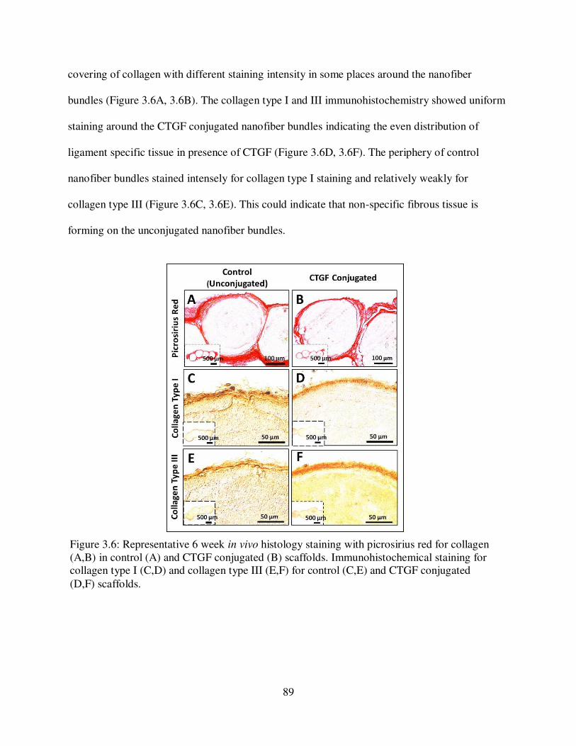
89

covering of collagen with different staining intensity in some places around the nanofiber

bundles (Figure 3.6A, 3.6B). The collagen type I and III immunohistochemistry showed uniform

staining around the CTGF conjugated nanofiber bundles indicating the even distribution of

ligament specific tissue in presence of CTGF (Figure 3.6D, 3.6F). The periphery of control

nanofiber bundles stained intensely for collagen type I staining and relatively weakly for

collagen type III (Figure 3.6C, 3.6E). This could indicate that non-specific fibrous tissue is

forming on the unconjugated nanofiber bundles.

Figure 3.6: Representative 6 week in vivo histology staining with picrosirius red for collagen (A,B) in control (A) and CTGF conjugated (B) scaffolds. Immunohistochemical staining for collagen type I (C,D) and collagen type III (E,F) for control (C,E) and CTGF conjugated

(D,F) scaffolds.

90

3.4 Discussion

The key requirements for a tissue engineered ligament scaffold have been well described

previously21,34. The scaffold must be made from a biocompatible material and closely match the

structural and mechanical properties of the native tissue. The scaffolds investigated in this work

represent a hierarchal construct that mimics the structure of the native human ACL using sheets

of aligned nanofibers prepared using a standard electrospinning technique. By rolling rectangular

sections of the electrospun nanofiber sheets to create nanofiber bundles it creates a robust

structure which supports cell growth and proliferation, cell elongation, and has material

properties that are comparable to the properties of the native human ACL16–18. Others have

attempted to use stacked PCL sheets for ACL replacement and while transient immune responses

were noted15, they subsided and the potential for heparin-mediated growth factor release was

noted, as a technique for further encouraging de novo extracellular matrix deposition35,36.

Similarly, Bosworth et al. reported that tightly wound PCL yarn could be utilized as a substrate

for tendon fibroblast adhesion and proliferation37. Modifications to traditional PCL have also

been investigated as materials for ligament scaffolds, particularly ultra-high molecular weight

PCL (UHMWPCL) and PCL with the addition of L-lactic acid (PCLC) with promising

results38,39. In the current study, a scaffold composed of multiple nanofiber bundles was created

to better mimic the hierarchal structure of the collagen in the native ACL on macro, micro, and

nano-size scales, and provide space for matrix deposition between and around the nanofiber

bundles.

In addition to scaffold material, it is also important to consider the structure of the scaffold. The

native ACL possess a complex hierarchical structure with collagen fibrils primarily oriented

91

along the longitudinal axis of the ligament20 and then organized into fascicles5. The primarily

parallel orientation is thought to lend tensile strength and stability to the ligament4. The scaffold

presented in this work was fabricated to attempt to mimic this hierarchical structure. The

electrospun PCL nanofibers which mimic the collagen fibrils are tightly rolled upon themselves

to create nanofiber bundles which mimic the collagen fascicles. Previous work showed that these

individual nanofiber bundles promoted cell adhesion and proliferation16. In order to provide a

suitable ligament replacement, a scaffold must also be able to withstand the repeated tensile

loading experienced by native ligaments. Previous mechanical testing revealed that when pulled

to failure at a physiologically relevant strain rate the modulus, yield stress, and yield stress and

yield strain of nanofiber bundles mimic the material properties of the native human ACL,

suggesting this scaffold has the potential to meet the mechanical demands of the ligament16. To

better mimic the overall ACL structure multiple nanofiber bundles were grouped together by

tying the ends together, which allows the nanofiber bundles to lie parallel to one another.

Although the native collagen fascicles of ACL are not perfectly parallel to one another,

particularly when comparing fascicles in the in the anteromedial and posterolateral bundles of

the ligament, this scaffold structure represents a first step at mimicking the hierarchical ACL

structure. Other groups have attempted to recreate the hierarchical ACL structure with various

techniques. Two popular techniques are utilizing braided or twisted strands of material to

increase stiffness and tensile strength, however encouraging cell infiltration can be

challenging13,39–42. A recent study comparing braided electrospun PCL sheets to stacked

electrospun PCL sheets showed that the braided scaffolds possessed improved tensile strength

which better mimicked the native ACL, however, cell infiltration and proliferation was superior

in stacked constructs43.

92

In order to encourage cell adhesion and proliferation as well as the deposition of native ligament

ECM by the cells, we investigated the chemical conjugation of growth factors on the surface of

the scaffold. The chemical conjugation technique used in this study resulted in a 95%

conjugation efficiency, which suggests a secure covalent bond between the PCL, linker

molecules, and the CTGF. After an initial burst release, over a two week time period only ~6%

of the conjugated CTGF was released from the scaffold. Previous studies using similar

techniques to covalently immobilize growth factors on scaffold surfaces have shown similar

release profiles28,44. The initial burst release of CTGF into the surrounding media could be due to

the release of some unconjugated CTGF that was physically trapped within the porous network

of nanofibers and required multiple days to diffuse out into the surrounding solution. The CTGF

that remains covalently conjugated to the nanofiber bundles is thought to influence cells that

adhere to the scaffold via juxtacrine signal transduction45. When cells are in contact with the

conjugated growth factors, signal transduction pathways are initiated which lead to cellular

adaptation and upregulation of collagen I and III production29.

After one week of in vitro culture, there was no difference in cell metabolic activity on nanofiber

bundles with and without conjugated with CTGF. Thus, for early time points, the presence of the

CTGF likely has no impact on cell proliferation and viability. Other groups that have utilized

growth factors for ligament tissue engineering have found differences in cell proliferation as

early as 7 days in vitro. Notably, after 1 week of culture Sahoo et al. demonstrated significantly

higher viability when cells were grown on knitted silk scaffolds that had been with electrospun

nanofibers made of a PLGA/basic fibroblastic growth factor (bFGF) blend, compared to the

same scaffolds without bFGF46. However, this response could be due to the release profile of the

93

bFGF since nearly 60% was released into the surrounding media in the first 7 days47. Similarly,

Hankemeier et al. showed that after 7 days of culture higher doses of bFGF results in a higher

density of cells48. On our scaffolds, no apparent differences in cell coverage on nanofiber bundle

surfaces were noted, and cells became elongated along the long-axis of the nanofiber bundle

regardless of CTGF presence. This is somewhat surprising since previous studies have shown

that the presence of CTGF induces a more elongated cell shape22,24 however it could be that the

aligned PCL nanofibers present in our scaffold encourage cell elongation regardless of growth

factor presence. The shape and morphology of cells, as dictated by the structure of the scaffold,

influence cell migration, and communication as well as cellular differentiation49. In the context

of ligament tissue engineering, an elongated spindle-shaped cell morphology mimics the

structure of native fibroblasts and is thought to be important for fibroblastic cellular

differentiation50,51.

In contrast to the cell proliferation seen on individual nanofiber bundles, when scaffolds

consisting of ~20 nanofiber bundles were cultured in vitro, there were significant differences in

cell proliferation in the presence of conjugated CTGF. As early as 1 day after cell seeding, DNA

content and cellular metabolic activity on scaffolds with conjugated CTGF were both nearly

double that of control scaffolds. This suggests that initially, the cells had a greater affinity for

attaching to scaffolds with conjugated CTGF. However, on individual nanofiber bundles, cells

adhered at equal levels regardless of CTGF presence. This could be due to the differences in the

macro-scale architecture of the scaffold. Since the 3D scaffold consisted of multiple nanofiber

bundles, each conjugated with CTGF, the larger area of exposed surface area for growth factor

could encourage more cell attachment. It is difficult to compare our initial cell attachment results

94

to those of other groups since typically cell behavior is not investigated after only one day of in

vitro culture. However, in the future, it will be necessary to better understand what chemical and

structural properties of scaffolds influence initial cell attachment. The trend for higher DNA

content and higher metabolic activity on CTGF scaffolds persisted through day 21 of in vitro

culture. Additionally, after 21 days of in vitro culture, the cell metabolic activity and the DNA

content on CTGF conjugated scaffolds was higher than it had been at day 1, suggesting robust

cellular proliferation throughout the 3 week culture period. These results closely match those of

other research groups who have assessed the proliferation of cells both in the presence of other

ligament-related growth factors35,46,48,52 and specifically in the presence of CTGF22,24.

In addition to influencing cell adhesion and proliferation, conjugated CTGF had an effect on the

matrix material deposited by cells in vitro. Collagen is the predominant extracellular matrix

material in ligaments and its presence is crucial for repair and regeneration of fibrous tissues53.

Robust deposition of collagen is vital for a successful tissue engineered ligament so that as the

scaffold gradually degrades, de novo tissue remains in its place. Cells on all scaffolds deposited

collagen around the nanofiber bundles. The collagen deposition was mostly observed around the

outside of the scaffold where it bridged the gaps between nanofiber bundles, however, some

collagen deposition was also present toward the interior of the scaffold. Similarly, Copper et al.

implanted braided scaffolds composed of PLLA fibers in a rabbit ACL reconstruction model and

noted robust deposition of cells and dense connective tissue surrounding all polymer fibers54.

The 21 day in vitro culture period investigated in the present study was chosen based on

measurable changes in collagen deposition between the groups of control and CTGF conjugated

scaffolds. Additionally, other research groups who have investigated the effects of growth factors

95

on nanofibrous scaffolds in vitro have used similar 3 week time points to investigate cell

behavior13,24,46,52,55. In order to further encourage more robust deposition of collagen around and

between the individual nanofiber bundles that compose the 3D scaffold it may be necessary to

incorporate mechanical stimulation. Previous groups have shown that compared to static culture,

tensile loading of polymer scaffolds during culture encourages more cellular deposition of highly

aligned collagen fibers similar to those observed in ligaments56,57. Additionally, nano-scale

alterations such as modifying the nanofibers to have a crimp-like microarchitecture may

encourage ECM deposition and cell differentiation58,59. On the scaffolds presented in this study,

collagen deposition was notably more pronounced on scaffolds with conjugated CTGF.

Quantitatively, the measured amount of accumulated collagen (normalized for DNA content)

was nearly 4 times higher on CTGF scaffolds compared to control scaffolds. CTGF presence has

been previously shown to stimulate the robust production of collagen in vitro in both fibroblasts

and mesenchymal stem cells based on assessment of mRNA levels and histological staining of

tissues22,23.

Ideally, the extracellular matrix produced by cells on a tissue-engineered ligament should mimic

the structure and biological function of the native ligament ECM as much as possible. Thus,

when considering collagen deposition on a scaffold it is important to not only note the presence

of collagen, but also the specific types of collagen. Collagen type I is the major collagen found in

ligaments however collagen type III is also present5. Type III collagen is found throughout the

ACL as a component of reticular fibers, a loose connective tissue that divides type I collagen

bundles. Immunohistochemistry after 3 weeks in vitro showed that on scaffolds with conjugated

CTGF the collagen that was deposited on the surface of the nanofiber bundles was primarily

96

types I and III. In contrast, on the control scaffolds, there was essentially no evidence of either

collagen I or III staining. There has been some evidence to suggest that the levels of different

types of collagen fluctuate during tendon development, where type III collagen is deposited

initially and later replaced by type I collagen60. Similarly, during the connective tissue healing

process, some groups have found an initial increase in type III collagen followed by additional

type I collagen deposition61,62. Thus in future work, it may be beneficial to quantify the types of

collagen present to assess early recapitulation of the ligament development and healing process.

Additionally, notable deposition of collagen types I and III could suggest that the OBMSCs

seeded on the scaffolds are beginning to differentiate into fibroblasts, cells characteristic of

ligaments63,64. In future studies, gene expression changes will be investigated to further confirm

cell differentiation.

There was no apparent deposition of calcium or sGAG on any scaffolds. The absence of calcium

is appropriate since no calcium is present in native ligaments. By Day 21 the amount of sGAG

accumulated on CTGF scaffolds was lower than the accumulated sGAG on control scaffolds.

Because high sGAG production is typically associated with chondrogenic differentiation, less

accumulation of sGAG further suggests that the OBMSCs seeded on the scaffolds conjugated

with CTGF may be differentiating into fibroblasts65. The ACL does have a small amount of

sGAG, about 9% of the weight of the dry tissue, which is thought to be important for the

viscoelastic mechanical behavior5,66. In future studies, it may be necessary to optimize the

amount of CTGF present in order to regulate the spatial deposition of both sGAG and collagen.

97

In an effort to better understand the in vivo response of cells to the scaffold and conjugated

growth factor at a long time point, a nude mouse model was utilized. The smaller size of the

scaffolds implanted in vivo permitted the assessment of matrix deposition between nanofiber

bundles while conserving space and resources. The 6 week implantation period was chosen in

order to be an extension of the in vitro time point and to get an initial indication of longer term in

vivo cell behavior. After 6 weeks of in vivo implantation, collagen deposition was observed

around all fibers of the scaffolds. The stacked electrospun PCL scaffold implanted in vitro by

Petrigliano et al. in a rat model of ACL reconstruction showed that cells did not start producing a

collagen matrix until 6 weeks after implantation, and this collagen matrix matured through week

1215. Thus it is possible that the collagen observed on our scaffolds in vitro would continue to

increase and mature with additional implantation time. For the scaffolds presented in this study,

in vivo collagen deposition appeared similar for both control and CTGF scaffolds. Differences in

the influence of CTGF on collagen deposition in vitro and in vivo could be due to the longer time

point, the presence of host cells in vivo, or the influence of other in vivo environmental cues.

Additionally, the collagen deposited on all scaffolds (control and CTGF conjugated) in vivo was

identified as collagen types I and III. This is a slightly different from what was observed in vitro,

where types I and III collagen were only identified on CTGF conjugated scaffolds. This

difference could be based on culture times, and potentially with longer in vitro, culture times

collagen I and III accumulation would increase on control scaffolds, similar to what was seen in

vivo. Similarly, a knitted silk scaffold implanted in a porcine ACL reconstruction model was

found to support robust deposition of collagen I and III and tenasin-C in vivo67. One limitation of

the in vivo results presented is a lack of quantification of collagen content of the scaffolds. Non-

specific fibrous tissue that can form around scaffolds during subcutaneous implantation can

98

interfere with the hydroxyproline assay which is commonly used to measure collagen content.

Thus we chose to only utilize histology and immunohistochemical staining for the specific types

of collagen found in ligaments. An additional limitation of the in vivo work is that in the in vivo

environment it is challenging to separate the activities of the cells seeded on the scaffold prior to

implantation from host cells found within the animal. For example, Spalazzi et al implanted a

triphasic polymer scaffold subcutaneously in an athymic rat and found thorough host cell

infiltration which led to the deposition of de novo tissue within the scaffold68,69. Future studies

will explore implanting cell-free and cell-laden scaffolds in more challenging orthotopic

locations.

Overall the results of this study have demonstrated that it is possible to utilize CTGF conjugation

and novel biofabrication strategies to create a bioactive scaffold that mimics the hierarchal

structure of the native ACL. During in vitro and in vivo culture the presence of CTGF

encourages cell adhesion, proliferation, and robust deposition of collagen which is specific for

ligament tissue. This suggests that the presence of CTGF may be influencing the seeded stem

cells to differentiate into ligamentous cells. Therefore the scaffold developed in this study, in

combination with CTGF and cells, could serve as a tissue engineered ACL replacement.

99

REFERENCES

1. Dye, S. F. & Cannon, W. D. Anatomy and biomechanics of the anterior cruciate ligament. Clin. Sports Med. 7, 715–25 (1988).

2. Girgis, F. G., Marshall, J. L. & Monajem, A. The cruciate ligaments of the knee joint. Anatomical, functional and experimental analysis. Clin. Orthop. Relat. Res. 216–31 (1975).

3. Woo, S. L., Hildebrand, K., Watanabe, N., Fenwick, J. a, Papageorgiou, C. D. & Wang, J. H. Tissue engineering of ligament and tendon healing. Clin. Orthop. Relat. Res. S312–S323 (1999).

4. Arnoczky, S. Anatomy of the anterior cruciate ligament. Clin. Orthop. Relat. Res. 172, 19–25 (1983).

5. Duthon, V. B., Barea, C., Abrassart, S., Fasel, J. H., Fritschy, D. & Ménétrey, J. Anatomy of the anterior cruciate ligament. Knee Surg. Sports Traumatol. Arthrosc. 14, 204–13 (2006).

6. Giugliano, D. N. & Solomon, J. L. ACL Tears in Female Athletes. Phys. Med. Rehabil.

Clin. N. Am. 18, 417–438 (2007).

7. Prodromos, C. C., Han, Y., Rogowski, J., Joyce, B. & Shi, K. A Meta-analysis of the Incidence of Anterior Cruciate Ligament Tears as a Function of Gender, Sport, and a Knee Injury-Reduction Regimen. Arthrosc. J. Arthrosc. Relat. Surg. 23, 1320–1325 (2007).

8. Buss, D. D., Warren, R. F., Wickiewicz, T. L., Galinat, B. J. & Panariello, R. Arthroscopically assisted reconstruction of the anterior cruciate ligament with use of autogenous patellar-ligament grafts. Results after twenty-four to forty-two months. J.

Bone Joint Surg. Am. 75, 1346–1355 (1993).

9. Langan, P. & Fontanetta, A. P. Rupture of the patellar tendon after use of its central third. Orthop. Rev. 16, 317–321 (1987).

10. Simonds, R. J., Holmberg, S. D., Hurwitz, R. L., Coleman, T. R., Bottenfield, S., Conley, L. J., Kohlenberg, S. H., Castro, K. G., Dahan, B. A. & Schable, C. A. Transmission of human immunodeficiency virus type 1 from a seronegative organ and tissue donor. N.

Engl. J. Med. 326, 726–732 (1992).

11. Pedicini, A. & Farris, R. J. Mechanical behavior of electrospun polyurethane. Polymer. 44, 6857–6862 (2003).

100

12. Li, D. & Xia, Y. Electrospinning of Nanofibers: Reinventing the Wheel? Adv. Mater. 16, 1151–1170 (2004).

13. Barber, J. G., Handorf, A. M., Allee, T. J. & Li, W.-J. Braided nanofibrous scaffold for tendon and ligament tissue engineering. Tissue Eng. Part A 19, 1265–74 (2013).

14. Freeman, J. W., Woods, M. D. & Laurencin, C. T. Tissue engineering of the anterior cruciate ligament using a braid-twist scaffold design. J. Biomech. 40, 2029–36 (2007).

15. Petrigliano, F. A., Arom, G. A., Nazemi, A. N., Yeranosian, M. G., Wu, B. M. & McAllister, D. R. In Vivo Evaluation of Electrospun Polycaprolactone Graft for Anterior Cruciate Ligament Engineering. Tissue Eng. Part A 21, 1228–2136 (2015).

16. Pauly, H. M., Kelly, D. J., Popat, K. C., Trujillo, N. a, Dunne, N. J., Mccarthy, H. O. & Donahue, T. L. H. Mechanical Properties and Cellular Response of Novel Electrospun Nanofibers for Ligament Tissue Engineering : Effects of Orientation and Geometry Reference : J. Mech. Behav. Biomed. Mater. 61, 258–270 (2016).

17. Skelley, N. W., Castile, R. M., Cannon, P. C., Weber, C. I., Brophy, R. H. & Lake, S. P. Regional Variation in the Mechanical and Microstructural Properties of the Human Anterior Cruciate Ligament. Am. J. Sports Med. 2892–2899 (2016). doi:10.1177/0363546516654480

18. Paschos, N. K., Gartzonikas, D., Barkoula, N. M., Moraiti, C., Paipetis, A., Matikas, T. E. & Georgoulis, A. D. Cadaveric Study of Anterior Cruciate Ligament Failure Patterns Under Uniaxial Tension Along the Ligament. Arthrosc. - J. Arthrosc. Relat. Surg. 26, 957–967 (2010).

19. Kastelic, J., Galeski, A. & Baer, E. The multicomposite structure of tendon. Connect.

Tissue Res. 6, 11–23 (1978).

20. Danylchuk, K. D., Finlay, J. B. & Krcek, J. P. Microstructural organization of human and bovine cruciate ligaments. Clin. Orthop. Relat. Res. 131, 294–298 (1978).

21. Petrigliano, F. A., McAllister, D. R. & Wu, B. M. Tissue engineering for anterior cruciate ligament reconstruction: a review of current strategies. Arthroscopy 22, 441–451 (2006).

22. Lee, C. H., Shah, B., Moioli, E. K. & Mao, J. J. CTGF directs fibroblast differentiation from human mesenchymal stem/stromal cells and defines connective tissue healing in a rodent injury model. J. Clin. Invest. 120, 3340–3349 (2010).

23. Moussad, E. E.-D. a. & Brigstock, D. R. Connective Tissue Growth Factor: What’s in a Name? Mol. Genet. Metab. 71, 276–292 (2000).

101

24. Tong, Z., Sant, S., Khademhosseini, A. & Jia, X. Controlling the Fibroblastic Differentiation of Mesenchymal Stem Cells Via the Combination of Fibrous Scaffolds and Connective Tissue Growth Factor. Tissue Eng. Part A 17, 2773–2785 (2011).

25. Lee, K., Silva, E. A. & Mooney, D. J. Growth factor delivery-based tissue engineering: general approaches and a review of recent developments. J. R. Soc. Interface 8, 153–70 (2011).

26. Yoo, H. S., Kim, T. G. & Park, T. G. Surface-functionalized electrospun nanofibers for tissue engineering and drug delivery. Adv. Drug Deliv. Rev. 61, 1033–1042 (2009).

27. Choi, J. S., Leong, K. W. & Yoo, H. S. In vivo wound healing of diabetic ulcers using electrospun nanofibers immobilized with human epidermal growth factor (EGF). Biomaterials 29, 587–596 (2008).

28. Mottaghitalab, F., Farokhi, M., Mottaghitalab, V., Ziabari, M., Divsalar, A. & Shokrgozar, M. A. Enhancement of neural cell lines proliferation using nano-structured chitosan/poly(vinyl alcohol) scaffolds conjugated with nerve growth factor. Carbohydr.

Polym. 86, 526–535 (2011).

29. Zhang, H., Migneco, F., Lin, C. Y. & Hollister, S. J. Chemically-conjugated bone morphogenetic protein-2 on three-dimensional polycaprolactone scaffolds stimulates osteogenic activity in bone marrow stromal cells. Tissue Eng. Part A 16, 3441–8 (2010).

30. Thorpe, S. D., Nagel, T., Carroll, S. F. & Kelly, D. J. Modulating Gradients in Regulatory Signals within Mesenchymal Stem Cell Seeded Hydrogels: A Novel Strategy to Engineer Zonal Articular Cartilage. PLoS One 8, 1–13 (2013).

31. Guillaume, O., Daly, A., Lennon, K., Gansau, J., Buckley, S. F. & Buckley, C. T. Shape-memory porous alginate scaffolds for regeneration of the annulus fibrosus: effect of TGF-β3 supplementation and oxygen culture conditions. Acta Biomater. 10, 1985–95 (2014).

32. Ignat’eva, N. Y., Danilov, N. a., Averkiev, S. V., Obrezkova, M. V., Lunin, V. V. & Sobol’, E. N. Determination of hydroxyproline in tissues and the evaluation of the collagen content of the tissues. J. Anal. Chem. 62, 51–57 (2007).

33. Vinardell, T., Sheehy, E. J., Buckley, C. T. & Kelly, D. J. A comparison of the functionality and in vivo phenotypic stability of cartilaginous tissues engineered from different stem cell sources. Tissue Eng. Part A 18, 1161–70 (2012).

34. Leong, N. L., Petrigliano, F. A. & McAllister, D. R. Current tissue engineering strategies in anterior cruciate ligament reconstruction. J. Biomed. Mater. Res. A 102, 1614–24 (2014).

35. Leong, N. L., Kabir, N., Arshi, A., Nazemi, A., Wu, B., Petrigliano, F. A. & McAllister, D. R. Evaluation of polycaprolactone scaffold with basic fibroblast growth factor and

102

fibroblasts in an athymic rat model for anterior cruciate ligament reconstruction. Tissue

Eng. Part A 21, 1859–68 (2015).

36. Leong, N. L., Arshi, A., Kabir, N., Nazemi, A., Petrigliano, F. A., Wu, B. M. & McAllister, D. R. In vitro and in vivo evaluation of heparin mediated growth factor release from tissue-engineered constructs for anterior cruciate ligament reconstruction. J. Orthop.

Res. 33, 229–236 (2015).

37. Bosworth, L. A., Alam, N., Wong, J. K. & Downes, S. Investigation of 2D and 3D electrospun scaffolds intended for tendon repair. J. Mater. Sci. Mater. Med. 24, 1605–14 (2013).

38. Leong, N. L., Kabir, N., Arshi, A., Nazemi, A., Jiang, J., Wu, B. M., Petrigliano, F. A. & McAllister, D. R. Use of ultra-high molecular weight polycaprolactone scaffolds for ACL reconstruction. J. Orthop. Res. 34, 828–835 (2016).

39. Laurent, C. P., Ganghoffer, J.-F., Babin, J., Six, J. L., Wang, X. & Rahouadj, R. Morphological characterization of a novel scaffold for anterior cruciate ligament tissue engineering. J. Biomech. Eng. 133, 011006 (2006).

40. Chung, E. J., Sugimoto, M. J., Koh, J. L. & Ameer, G. A. A biodegradable tri-component graft for anterior cruciate ligament reconstruction. J. Tissue Eng. Regen. Med. 4, (2014).

41. Cooper, J. A., Lu, H. H., Ko, F. K., Freeman, J. W. & Laurencin, C. T. Fiber-based tissue-engineered scaffold for ligament replacement: design considerations and in vitro evaluation. Biomaterials 26, 1523–32 (2005).

42. Lu, H. H., Cooper, J. A., Manuel, S., Freeman, J. W., Attawia, M. A., Ko, F. K. & Laurencin, C. T. Anterior cruciate ligament regeneration using braided biodegradable scaffolds: in vitro optimization studies. Biomaterials 26, 4805–16 (2005).

43. Rothrauff, B. B., Lauro, B. B., Yang, G., Debski, R. E., Musahl, V. & Tuan, R. Braided and Stacked Electrospun Nanofibrous Scaffolds for Tendon and Ligament Tissue Engineering. Tissue Eng. Part A (2017).

44. Cho, Y. Il, Choi, J. S., Jeong, S. Y. & Yoo, H. S. Nerve growth factor (NGF)-conjugated electrospun nanostructures with topographical cues for neuronal differentiation of mesenchymal stem cells. Acta Biomater. 6, 4725–4733 (2010).

45. Liu, H. W., Chen, C. H., Tsai, C. L. & Hsiue, G. H. Targeted delivery system for juxtacrine signaling growth factor based on rhBMP-2-mediated carrier-protein conjugation. Bone 39, 825–836 (2006).

46. Sahoo, S., Toh, S. L. & Goh, J. C. H. A bFGF-releasing silk/PLGA-based biohybrid scaffold for ligament/tendon tissue engineering using mesenchymal progenitor cells. Biomaterials 31, 2990–2998 (2010).

103

47. Sahoo, S., Ang, L. T., Goh, J. C. H. & Toh, S. L. Growth factor delivery through electrospun nanofibers in scaffolds for tissue engineering applications. J. Biomed. Mater.

Res. A 93, 1539–1550 (2010).

48. Hankemeier, S., Keus, M., Zeichen, J., Jagodzinski, M., Barkhausen, T., Bosch, U., Krettek, C. & Van Griensven, M. Modulation of proliferation and differentiation of human bone marrow stromal cells by fibroblast growth factor 2: potential implications for tissue engineering of tendons and ligaments. Tissue Eng. 11, 41–49 (2005).

49. Kilian, K. A., Bugarija, B., Lahn, B. T. & Mrksich, M. Geometric cues for directing the differentiation of mesenchymal stem cells. Proc. Natl. Acad. Sci. U. S. A. 107, 4872–4877 (2010).

50. Wells, R. G. The role of matrix stiffness in regulating cell behavior. Hepatology 47, 1394–1400 (2008).

51. Subramony, S. D., Dargis, B. R., Castillo, M., Azeloglu, E. U., Tracey, M. S., Su, A. & Lu, H. H. The guidance of stem cell differentiation by substrate alignment and mechanical stimulation. Biomaterials 34, 1942–53 (2013).

52. Petrigliano, F. A., English, C. S., Barba, D., Esmende, S., Wu, B. M. & McAllister, D. R. The effects of local bFGF release and uniaxial strain on cellular adaptation and gene expression in a 3D environment: implications for ligament tissue engineering. Tissue Eng. 13, 2721–31 (2007).

53. Lin, T. W., Cardenas, L. & Soslowsky, L. J. Biomechanics of tendon injury and repair. J.

Biomech. 37, 865–877 (2004).

54. Cooper, J. A., Sahota, J. S., Gorum, W. J., Carter, J., Doty, S. B. & Laurencin, C. T. Biomimetic tissue-engineered anterior cruciate ligament replacement. Proc. Natl. Acad.

Sci. U. S. A. 104, 3049–54 (2007).

55. Bosworth, L. A., Rathbone, S. R., Bradley, R. S. & Cartmell, S. H. Dynamic loading of electrospun yarns guides mesenchymal stem cells towards a tendon lineage. J. Mech.

Behav. Biomed. Mater. (2014). doi:10.1016/j.jmbbm.2014.07.009

56. Nerurkar, N. L., Sen, S., Baker, B. M., Elliott, D. M. & Mauck, R. L. Dynamic culture enhances stem cell infiltration and modulates extracellular matrix production on aligned electrospun nanofibrous scaffolds. Acta Biomater. 7, 485–91 (2011).

57. Teuschl, A., Heimel, P., Nürnberger, S., Van Griensven, M., Redl, H. & Nau, T. A novel silk fiber-based scaffold for regeneration of the anterior cruciate ligament: Histological results from a study in sheep. Am. J. Sports Med. 44, 1547–1557 (2016).

104

58. Chen, F., Hayami, J. W. S. & Amsden, B. G. Electrospun poly(l -lactide-co -acryloyl carbonate) fiber scaffolds with a mechanically stable crimp structure for ligament tissue engineering. Biomacromolecules 15, 1593–1601 (2014).

59. Surrao, D. C., Fan, J. C. Y., Waldman, S. D. & Amsden, B. G. A crimp-like microarchitecture improves tissue production in fibrous ligament scaffolds in response to mechanical stimuli. Acta Biomater. 8, 3704–13 (2012).

60. Tozer, S. & Duprez, D. Tendon and ligament: Development, repair and disease. Birth

Defects Res. Part C - Embryo Today Rev. 75, 226–236 (2005).

61. Eriksen, H. A., Pajala, A., Leppilahti, J. & Risteli, J. Increased content of type III collagen at the rupture site of human Achilles tendon. J. Orthop. Res. 20, 1352–1357 (2002).

62. Amiel, D., Frank, C. B., Harwood, F. L., Akeson, W. H. & Kleiner, J. B. Collagen Alteration in Medial Collateral Ligament Healing in a Rabbit Model. Connect. Tissue Res. 16, 357–366 (1987).

63. Altman, G. H., Horan, R. L., Lu, H. H., Moreau, J., Martin, I., Richmond, J. C. & Kaplan, D. L. Silk matrix for tissue engineered anterior cruciate ligaments. Biomaterials 23, 4131–41 (2002).

64. Fan, H., Liu, H., Toh, S. L. & Goh, J. C. H. Enhanced differentiation of mesenchymal stem cells co-cultured with ligament fibroblasts on gelatin/silk fibroin hybrid scaffold. Biomaterials 29, 1017–1027 (2008).

65. Barry, F., Boynton, R. E., Liu, B. & Murphy, J. M. Chondrogenic Differentiation of Mesenchymal Stem Cells from Bone Marrow: Differentiation-Dependent Gene Expression of Matrix Components. Exp. Cell Res. 268, 189–200 (2001).

66. Amiel, D., Frank, C., Harwood, F., Fronek, J. & Akeson, W. Tendons and ligaments: a morphological and biochemical comparison. J. Orthop. Res. 1, 257–65 (1984).

67. Fan, H., Liu, H., Wong, E. J. W., Toh, S. L. & Goh, J. C. H. In vivo study of anterior cruciate ligament regeneration using mesenchymal stem cells and silk scaffold. Biomaterials 29, 3324–37 (2008).

68. Spalazzi, J. P., Doty, S. B., Moffat, K. L., Levine, W. N. & Lu, H. H. Development of controlled matrix heterogeneity on a triphasic scaffold for orthopedic interface tissue engineering. Tissue Eng. 12, 3497–508 (2006).

69. Mosher, C. Z., Spalazzi, J. P. & Lu, H. H. Stratified scaffold design for engineering composite tissues. Methods 84, 99–102 (2015).

105

CHAPTER 4:

MECHANICAL PROPERTIES OF A HIERARCHICAL ELECTROSPUN SCAFFOLD

FOR OVINE ANTERIOR CRUCIATE LIGAMENT REPLACEMENT

4. 1 Introduction

The anterior cruciate ligament (ACL) is a complex hierarchical structure that connects the femur

to the tibia and is composed primarily of collagen. The primary function of the ACL is to restrict

translations and rotations of the tibia and thus stabilize the knee throughout the functional range

of motion1. When the ACL is intact it prevents the tibia from displacing anteriorly relative to the

femur as well as undergoing excessive internal and varus-valgus tibial rotations2. When anterior

force is applied to the tibia of an ACL deficient knee, the anterior tibial translation is four times

greater than in an intact knee3,4. Clinically, functional stability is assessed using an anterior

drawer test5,6. The ACL is loaded throughout the gait cycle and musculoskeletal modeling has

shown that in human knees the ACL experiences peak loads of ~300 N and maximum strains of

approximately 3%7,8.

Similar to other tendons and ligaments, the ACL is characterized by nonlinear behavior in

response to applied tensile loads9. Under initial tensile loads, the force-displacement curve of the

ACL displays a characteristic low stiffness linear region where the collagen fibers of the

ligament are not yet loaded whereas the elastin component is loaded. Next, a non-linear toe

region is evident from the reversible un-crimping of collagen fibers, followed by a linear elastic

region of loading where the collagen fibers are completely un-crimped and taut10. The ACL also

exhibits time-dependent viscoelastic properties, where the elongation of the ligament depends

106

not only on the magnitude of the force but also on the application rate11. This time dependence is

often manifested as stress relaxation where the tissue shows a decrease in load under constant

elongation. These time-dependent material properties enable to ACL to contribute to knee

stability12.

Tears of the ACL are common and frequently occur during non-contact sports injuries13,14. In an

ACL deficient knee, altered joint kinematics can limit normal activities15. Following rupture of

the ACL, significant pain, bone bruising, joint instability, and damage to surrounding soft tissues

will occur16. ACL reconstruction aims to restore a connection between the femur and tibia to

restore stability to the joint17. Both allografts and autografts are commonly used to replace the

torn ACL15,18. Commonly used grafts include the semitendinosus tendon, the gracilis tendon, the

Achilles tendon, or patellar tendon with attached bone plugs19–21. Regardless of tissue type or

tissue source no definitive evidence has demonstrated the ability of ACL reconstructions to fully

restore knee functionally or prevent re-tears of the reconstruction or the contralateral ACL22–24.

Poor outcomes after ACL reconstruction may be attributed to a failure to match the mechanical

property of the native ACL and an inability of the reconstruction to restore knee kinematics25.

Additionally surgeons typically fail to treat occult damage that has occurred to surrounding

tissues, including tears of the menisci and damage to articular cartilage and subchondral bone,

which can result in accelerated osteoarthritis progression23.

Based on the limitations of traditional ACL allografts and autografts, our group has developed a

polycaprolactone (PCL) scaffold for use as a tissue-engineered ACL replacement that mimics the

hierarchical structure of the native ACL. PCL has a slow degradation rate and does not generate

107

harmful byproducts, making it a popular choice for tissue engineered scaffolds26. The scaffold

structure mimics a bone-patellar tendon-bone ACL graft with electrospun nanofiber bundles

connecting two solid cylindrical blocks intended to be inserted into bone tunnels. We have

previously shown that the sub-structural components of the scaffold mimic the hierarchical

structure and material properties of the native ACL27. Additionally, we have shown that ovine

bone marrow-derived stem cells seeded on the scaffold deposit collagen in vitro, and

implantation into the ovine stifle joint is clinically feasible28. Taken together, these advances

suggest that the novel scaffold could perform well as a tissue engineered ACL replacement.

Prior to an in vivo study, assessment of the scaffold ex vivo (prior to implantation) as well as in

situ (after implantation into a cadaver stifle joint) is necessary. Additionally, comparing the

performance of the implanted scaffold to an implanted soft tissue graft which mimics a “gold

standard” allograft or autograft would be beneficial. If the in situ performance of the implanted

scaffold is comparable to the performance of a traditional soft tissue graft, it would suggest that

the novel scaffold developed in this study can provide a similar amount of stabilization to the

knee as a current gold standard repair. Thus, the goal of this work was to evaluate the

performance of the novel scaffold as an ACL replacement.

4.2 Methods

4.2.1 Electrospun Scaffold Fabrication

The base material for the scaffolds (Figure 4.1A) was flat sheets of aligned electrospun

polycaprolactone (PCL) nanofibers created using a previously detailed electrospinning

technique27,28. Briefly, a 10% w/v solution of PCL (MW=80,000; Sigma 440744, St. Louis, MO)

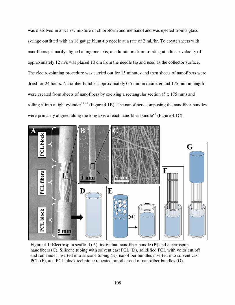
108

was dissolved in a 3:1 v/v mixture of chloroform and methanol and was ejected from a glass

syringe outfitted with an 18 gauge blunt-tip needle at a rate of 2 mL/hr. To create sheets with

nanofibers primarily aligned along one axis, an aluminum drum rotating at a linear velocity of

approximately 12 m/s was placed 10 cm from the needle tip and used as the collector surface.

The electrospinning procedure was carried out for 15 minutes and then sheets of nanofibers were

dried for 24 hours. Nanofiber bundles approximately 0.5 mm in diameter and 175 mm in length

were created from sheets of nanofibers by excising a rectangular section (5 x 175 mm) and

rolling it into a tight cylinder27,28 (Figure 4.1B). The nanofibers composing the nanofiber bundles

were primarily aligned along the long axis of each nanofiber bundle27 (Figure 4.1C).

Figure 4.1: Electrospun scaffold (A), individual nanofiber bundle (B) and electrospun nanofibers (C). Silicone tubing with solvent cast PCL (D), solidified PCL with voids cut off and remainder inserted into silicone tubing (E), nanofiber bundles inserted into solvent cast PCL (F), and PCL block technique repeated on other end of nanofiber bundles (G).

109

A solvent casting technique was used to combine together multiple nanofiber bundles to create a

complete scaffold (Figure 4.1D-G) Groups of approximately 50 nanofiber bundles with an

overall diameter of approximately 4 mm were cut to 35 mm in length and tied together with

sutures. The solvent solution was created by dissolving 3.5 mg PCL (Mw=50,000; Perstorp Capa

6506, Malmo, Sweden) in 5 mL of dichloromethane (Fisher Chemical D37-1) to create a 70%

w/v PCL solution. To create PCL blocks with diameter 6 mm and length 30 mm, 850 mL of the

PCL solution was cast into a segment of silicone tubing (Figure 4.1D) and the solvent was

allowed to evaporate off overnight. The upper 15 mm of each PCL block was cut off and

discarded due to the presence of voids formed from bubbles during solvent evaporation (Figure

4.1E). The remaining 15 mm of each PCL block was inserted into the bottom of a new segment

of silicone tubing (20 mm in length, Figure 4.1E) and 140 mL of 70% PCL solution was cast

onto the top of the PCL block. Immediately after casting the solution on top of the PCL block,

one end of the nanofiber bundle group was inserted into the solution (Figure 4.1F). The solvent

was allowed to evaporate overnight before repeating the procedure on the other end of the

nanofiber bundle group (Figure 4.1G). This procedure created scaffolds with a fiber region 4 mm

in diameter and 20 mm in length held together at each end with PCL blocks 6mm in diameter

and 20 mm in length (Figure 4.1A). The fiber region mimics the length of the native ovine ACL

to extend through the intraarticular space and the PCL blocks will be inserted into bone tunnels

in the femur and tibia.

4.2.2 Surgical technique

Ovine cadaver stifle joints were used for the study, and either a soft tissue allograft or a novel

electrospun scaffold was implanted for ACL reconstruction. “Gold standard” soft tissue grafts

110

were obtained by harvesting the lateral digital extensor (LDE) tendons from the hind limbs of

sheep (Ovis aris Rambouillet X Columbian ewes) that had been euthanized for unrelated

purposes. Hind limbs underwent one freeze thaw cycle prior to tendon harvest. Surgical

procedures were performed by trained veterinary surgeons. The LDE tendon was first isolated at

the metatarsal and then transected from the tibia. Harvested tendons were doubled looped and the

ends were augmented with sutures (Covidien, Polysorb 2-0). Soft tissue grafts were

approximately 6 mm in diameter and 120 mm in length and remained hydrated with phosphate

buffered saline solution (PBS) until use.

Prior to ACL reconstruction, the native ACL was transected and all remnant tissue was removed

so the femoral and tibial ACL footprints could be visualized. With the stifle joint flexed to

approximately 110º, the tibial bone tunnel was created such that the tunnel originated at the tibial

footprint of the ACL and emerged on the distal medial tibia. A 2.4 mm guide wire (Arthrex AR-

1250SB) was first drilled “inside-out” through the tibia and then a 7 mm tunnel was drilled over

the guide wire with an acorn reamer (Arthrex AR-1407-LP) to create a tibial bone tunnel

approximately 35 mm in length. With the joint still partially flexed the femoral bone tunnel was

drilled originating at the femoral footprint of the ACL and emerging on the proximal lateral

femur. A similar process was used to create a femoral bone tunnel approximately 30 mm in

length. Both bone tunnels were notched on the anterior margin and tapped with a 7mm tap to aid

interference screw insertion. Care was taken to avoid damaging any surrounding ligaments,

particularly the PCL and the intermeniscal ligament, as well as the anterior lateral meniscal root

during implantation of the ACL replacement.

111

For implantation of the soft tissue allograft, the graft was first delivered into the femoral bone

tunnel using a passing pin. With the joint in high flexion, a 7 mm stainless steel interference

screw (Arthrex AR-1370H-25) was inserted “inside-out” into the posterior-medial aspect of the

femoral tunnel while the graft was tensioned on the posterio-lateral aspect of the tunnel. The free

end of the graft was then delivered into the tibial bone tunnel and care was taken to ensure the

graft did not twist in the intraarticular space. With the joint at approximately 90º of flexion and

the graft tensioned along the postero-lateral aspect of the tibial bone tunnel, a 7 mm interference

screw was inserted “inside-out” into the antero-medial aspect of the tibial bone tunnel.

For implantation of electrospun scaffold, fishing line was inserted through each PCL block to

serve as passing sutures. A passing pin was used to draw the scaffold “outside-in” through the

tibial bone tunnel so that the one PCL block remained in the tibial tunnel. The second PCL block

was drawn “inside-out” through the femoral tunnel with the passing pin and care was taken to

ensure that the fibers were not twisted in the intraarticular space. With the joint in high flexion

and tension on the scaffold via the tibial passing sutures, a 6 mm stainless steel interference

screw (Arthrex AR-1360E) was inserted “inside-out” into the antero-medial aspect of the

femoral bone tunnel. Finally with the joint at approximately 90º of flexion and the graft

tensioned via the tibial passing sutures, a 6 mm interference screw was inserted “inside-out” into

the antero-medial aspect of the tibial bone tunnel.

4.2.3 Ovine stifle joint mechanical testing

Ovine cadaver stifle joints were obtained from sheep (Ovis aris Rambouillet X Columbian ewes)

that had been euthanized for unrelated studies. Stifle joints were tested under four conditions:

112

ACL intact (ACL), ACL transected (ACLX), soft tissue graft implanted (Graft), and electrospun

scaffold implanted (Scaffold in situ). Surgical techniques for soft tissue graft and electrospun

scaffold implantation are described above. Prior to mechanical testing, the femur and tibia were

cut to approximately 135 mm from the stifle joint line and the proximal 70 mm of the femur and

the distal 70 mm of the tibia were cleared of all tissue. Wood screws were drilled into the

proximal femur and distal tibia to increase surface area and the ends of the bones were potted in

resin (Smooth-Cast 321) in cylindrical cardboard molds (50 mm diameter, 70 mm length).

Stifle joints were tested using a servo-hydraulic material test system (MTS, Bionic Model 370.02

MTS Systems Corporation, Eden Prairie, MN). Anterior drawer testing was simulated for four

conditions: ACL intact (n=5), ACL transected (n=5), soft tissue graft implanted (n=6), and

electrospun scaffold implanted (n=6). Major stifle ligaments and the menisci were left intact

while all musculature was removed. The MTS was equipped with a 2000 lb load cell (Interface

1210AF-2k, Scottsdale, AZ) and a custom-built testing fixture was used to hold the joint at 90º

of flexion with the tibia positioned horizontally and the femur positioned vertically (Figure

4.2A). Following the application of a 5 N pre-load the femur was displaced upward at a rate of 1

mm/s (to mimic anterior tibial displacement) until 50 N of load was observed, as previously

described29–31.

113

Joints were then tested under stress relaxation followed by pull to failure testing for ACL intact

(n=5), soft tissue graft implanted (n=4), and electrospun scaffold implanted (n=5). Joints were

dissected of all soft tissue leaving only the ACL, soft tissue graft, or electrospun scaffold

attached at both the femoral and tibial insertions. With the stifle joint in full extension, calipers

were used on the posterior aspect of the joint to measure the length of the ACL, soft tissue graft,

or electrospun scaffold based on the distance from the center of the femoral insertion to the

center of the tibial insertion. The MTS was equipped with a 2000 lb load cell and a custom-built

testing fixture was used to hold the joint at 60º of flexion with the tibia positioned vertically to

ensure that the longitudinal axis of the ACL was aligned with the axis of loading29 (Figure 4.2B).

Joints were pre-loaded and then strained to 3% strain at a rate of 2mm/s, and held for 20 minutes

to record stress relaxation behavior. Preliminary testing showed that after 15 minutes the

Figure 4.2: Mechanical testing setup for simulated anterior drawer test (A), and stress relaxation and pull to failure tests (B).

114

observed load changed less than 0.1% over 1 minute indicating full relaxation had occurred.

Following stress relaxation testing, and a 10 minute rest period, a 5 N preload was applied and

the tibia was displaced upwards at a strain rate of 1%/sec until failure, which mimics the strain

rate of the native ACL during gait8,32.

4.2.4 Electrospun scaffold mechanical testing

Uniaxial tensile testing was performed on ex vivo electrospun scaffolds using a servo-hydraulic

material test system (MTS, Bionic Model 370.02 MTS Systems Corporation, Eden Prairie, MN)

equipped with a 100 lb load cell (Interface 1500ASK-100, Scottsdale, AZ). Hydraulic wedge

grips (Model 647 MTS Systems Corporation, Eden Prairie, MN) set to 500 psi were utilized to

clamp the PCL blocks at the base of the nanofiber bundles such that all strain occurred in the

fiber region. Sample gauge length was measured using a CCD camera (Flea3, Point Gray

Research, Richmond, BC, Canada). Stress relaxation and pull to failure tests were completed on

these samples under the same conditions described above for in situ testing.

4.2.5 Data analysis

Custom Matlab (R2016b Mathworks Inc., Natick, MA) codes were used to analyze the data. The

amount of displacement necessary to reach a load of 50 N was calculated as a measure of joint

laxity under the anterior drawer tests. Peak force was determined from the stress relaxation tests

as the maximum force reached during the test and the relaxation force was an average of the

force readings from 18 minutes – 20 minutes. Percent relaxation was calculated as the difference

between the peak force and relaxation force as a percent of the peak force. With the Matlab

Curve Fitting Toolbox, a second order power law fit of the force vs. time graph was used to fit

115

the relaxation curve. Equation 1 shows the equation used for fitting where y is equal to the force,

x is equal to the time, and the coefficients A, B, and C are obtained from the curve fit33–35.

Failure load and displacement values were determined from the pull to failure tests based on the

point at which the sample reached the maximum force. Strains were determined using the

original graft length. Using a least squares method, a bilinear curve fit was applied to the force-

displacement data to quantify the stiffness in the toe and linear regions, as well as force,

displacement, and strain values corresponding to the transition point of the bilinear fit36–38.

= � � + � (1)

Data are presented as mean ± standard deviation. For all quantitative measures, comparisons

were performed using multi-way analysis of variance (ANOVA) models with Tukey’s post-hoc

test using Minitab (Minitab, Inc., State College, PA). Differences corresponding to a p-value of

less than 0.05 were considered to be significant.

4.3 Results

4.3.1 Anterior drawer testing

Ovine cadaver stifle joints with the native ACL intact underwent 2.3mm of displacement to

reach an applied load of 50 N (Figure 4.3). After ACL transection, joint laxity increased

significantly compared to the intact ACL condition. Implantation of the electrospun scaffold

significantly reduced joint laxity compared to the ACLX condition and was not significantly

different than the ACL intact condition. In contrast, the soft tissue graft unable to restore joint

laxity to the native ACL and was not significantly different from the ACL transected condition.

116

4.3.2 Stress relaxation testing

The native ACL relaxed on average 36% over the 20 minute hold period. The scaffold ex vivo,

scaffold in situ, and the soft tissue graft relaxed 31%, 32%, and 63%, respectively, on average.

There were no statistically significant differences in the peak force or relaxation forces of the

native ACL and the scaffold ex vivo (Figure 4.4A). For the scaffold in situ, the peak force and

relaxation force were significantly lower than the native ACL. The soft tissue graft had a

relaxation force that was significantly lower than the native ACL. Using a second order power

law, the average curve fit had an R2 value of 0.96 ± 0.04 for the native ACL, 0.99 ± 0.01 for the

scaffold ex vivo, 0.97 ± 0.02 for the scaffold in situ, and 0.97 ± 0.03 for the soft tissue graft. No

statistically significant differences were found between the fitted coefficients of the native ACL

and the scaffolds ex vivo or in situ (Figures4.4B-D). However, all three of the fitted coefficients

of the graft samples were significantly different than all other groups (Figures 4.4B-D).

Figure 4.3: Anterior drawer laxity results. * Indicates significantly different from ACL (p<0.05), # indicates significantly different from ACLX (p<0.05).

117

Figure 4.4: Stress relaxation results including peak and relaxation force and second-order power law fitting coefficients. * Indicates significantly different from ACL (p<0.05), % indicates significantly different from scaffold ex vivo at (p<0.05), and $ indicates significantly different from scaffold in situ (p<0.05).

118

4.3.3 Pull to failure testing

The failure load of the native ACL was significantly greater than the scaffold ex vivo, the

scaffold in situ, and the soft tissue graft (Figure 4.5A, Figure 4.6), however, there were no

significant differences in the failure strain and failure displacement of any groups (Figure 4.5B,

4.5C). Bilinear fitting was applied to the native ACL and scaffold groups to quantify stiffness in

the toe and linear regions. Graft samples did not display an obvious toe region and thus only a

linear stiffness is reported. The toe region stiffness of the scaffold in situ was significantly lower

than the native ACL (Figure 4.7A). The stiffness of the ACL in the linear region was

significantly higher than the scaffold ex vivo, the scaffold in situ, and the graft (Figure 4.7A).

The force corresponding to the transition point from the toe region to linear region was

significantly higher for the native ACL compared to the scaffold ex vivo and in situ, however,

there were no differences in the transition displacements or strains (Figure 4.7B-D).

Figure 4.5: Pull to failure results including failure load (A), failure displacement (B), and failure strain (C). * Indicates significantly different from ACL (p<0.05).

119

Figure 4.6: Representative force displacement curves of native ACL, scaffold ex vivo, scaffold in situ, and soft tissue graft.

Figure 4.7: Toe and linear stiffness (A), transition load (B), transition displacement (C), and transition strain (D). * Indicates significantly different from ACL (p<0.05).

120

4.4 Discussion

In this study, we have developed a technique to simulate a clinical anterior drawer test which

provides a functional assessment of joint laxity. Similar to other studies on ovine limbs, an intact

ACL resulted in minimal displacement of the tibia relative to the femur and transection of the

ACL nearly tripled the amount of joint laxity29–31. Implantation of the soft tissue graft that was

used to mimic a “gold standard” tendon allograft failed to improve laxity levels and the joint

laxity was no different than when the ACL was transected. Studies have shown that a variety of

allograft materials are able to restore normal levels of joint laxity in cadaver knees during

simulated anterior drawer tests39,40. The sustained joint laxity observed with soft tissue graft in

the present study may be due to the graft fixation technique, or damage to the graft during

implantation. Studies comparing soft tissue graft fixation techniques have shown that fixation

with a transcondylar device or sutures secured over a button may provide a more robust repair

and mitigate damage to the graft during insertion41–44.

In contrast to the soft tissue graft, implantation of the electrospun scaffold improved joint laxity

by 50% and returned it back to normal (ACL intact) levels. It is likely that the secure attachment

of the PCL blocks and stainless steel interference screws in the bone tunnels contributed to the

reduced joint laxity. In an in vivo setting, this ability to decrease joint laxity will potentially

improve joint stability, decrease the risk of repair failure, and mitigate damage to surrounding

soft tissues16,45. Simulated anterior drawer testing has been previously used to assess the integrity

of tissue engineered ovine ACL replacements and decreased laxity after reconstruction has been

taken as an indication of biomechanical success of the tissue engineered ACL replacement29,31.

121

Stress relaxation experiments were utilized to compare the time-dependent properties of the

native ACL as well as the scaffold and soft tissue graft ACL replacements and the scaffold ex

vivo. Assessing the properties of the scaffold ex vivo provides a baseline measure of properties

without effects of surgical implantation or the in situ environment. Although the peak and

relaxation force of the native ACL and the scaffold ex vivo were in not significantly different,

after in situ implantation the scaffold demonstrated significantly lower peak and relaxation forces

than the native ACL. These differences in scaffold properties before and after implantation may

suggest that the implantation procedure is damaging the scaffold. Placement of the scaffold into

the bone tunnels requires significant physical manipulation which could be causing plastic

deformation of the nanofibers, thus reducing stiffness and diminishing the ability to support

applied loads. Additionally when the interference screws are inserted the sharp threads of the

screw may slice through some nanofibers on the periphery of the scaffold which would change

the structural properties. Future work should focus on optimizing the surgical procedure to

ensure the structural integrity of the scaffold is not compromised during implantation

The power-law fit of the stress relaxation curve demonstrated similar relaxation behavior

between the native ACL and the electrospun scaffold, suggesting that in vivo the scaffold may

mimic the time-dependent properties of the native ACL. In comparison, the fitted coefficients of

the soft tissue graft stress relaxation curve suggest that the soft tissue graft relaxes more quickly

than the native ACL. The graft also experienced nearly double the amount of relaxation as the

ACL in the same time period. The stress relaxation response of the ACL is important for the

ability of the ACL to prevent fatigue and stabilize the knee during prolonged joint motion and

thus an ACL replacement should possess similar time-dependent properties46.

122

In order to choose a suitable replacement for a damaged ACL, other groups have investigated the

time-dependent properties of soft tissue grafts via mechanical testing. Two variations of

semitendinosus grafts were tested via stress relaxation and demonstrated approximately 55%

relaxation47. This value closely matches the soft tissue graft in the present study however the

semitendinosus grafts were tested ex vivo so it is difficult to estimate the relaxation after

implantation. Donahue et al also performed testing on ex vivo soft tissue grafts from two species:

bovine and human48. Double looped bovine digital extensor tendons and human semitendinosus

and gracilis tendons demonstrated similar stress relaxation characteristics and relaxed

approximately 20%. This lower amount of relaxation may be due to the rigorous

preconditioning regime or variations in testing setup. Clinically it has been shown that graft

tension and stiffness achieved immediately following ACL reconstruction is not maintained post-

operatively due to stress relaxation, further emphasizing the importance of considering the stress

relaxation response when choosing materials for ACL reconstructions49.

Neither the electrospun scaffold (ex vivo or in vivo) nor the soft tissue graft was able to approach

the failure load of the native ACL. This is similar to other research groups whose ovine ACL

repair materials have been deficient in failure properties both before and after implantation50–53.

However, assessing the properties of ACL replacements via pull to failure tests may not provide

an accurate portrayal of in vivo behavior because the native ACL is not isolated and loaded in

pure tension to the point of failure during normal activities of daily living. Because the ACL

experiences strains of ~3% or ~1 mm during normal gait, investigating the behavior of ACL

replacements in the region of more functionally applicable smaller strains may be more relevant

for assessing the ability of replacements to mimic the native ACL. Hence, a bilinear fitting

123

approach was utilized to quantify two separate regions of the force-displacement curve: an initial

non-linear toe region, followed by a stiffer linear region that occurred at higher strains9. Both the

ACL and electrospun scaffold displayed the characteristic toe and linear regions. It is important

to note that the toe region stiffness of the ex vivo scaffold was not significantly different than the

toe region stiffness of the native ACL. This is promising as it suggests that in this lower strain

functional toe region, the scaffold performs similarly to the native ACL. The lower toe region

stiffness of the scaffold in situ may be due to rupture or plastic deformation of the nanofiber

bundles during surgical implantation. The soft tissue graft did not display a characteristic toe and

linear region which was surprising since tendon has been previously characterized as a

hyperelastic material54.

The bilinear fitting approach also permits identification of the transition point from the toe to

linear region. Transition displacement and strain values for the native ACL and scaffolds were

not different, and the transition strain is higher than the strains experienced by the native ACL in

vivo, which is expected since in vivo loading of the ACL occurs primarily in the toe region of the

force curve8,12. The transition force of the scaffold was significantly lower than the transition

force of the native ACL, suggesting that the scaffold begins to undergo plastic deformation at

lower loads. However, the transition force of the scaffold, as well as the toe region stiffness, are

expected to increase with in vivo implantation time and de novo tissue deposition55–57.

Overall the toe region and transition point similarities between the native ACL and the scaffold

may be attributed to the materials’ similar hierarchical structures. The viscoelastic behavior of

the ACL is thought to be due primarily to the crimped collagen fibers that make up the

124

ligament10. In the toe region of the force curve, the collagen fibers are experiencing reversible

un-crimping and it’s not until the linear region of that force-displacement curve that the collagen

fibers are fully un-crimped and directly loaded. Similarly, the electrospun scaffold is composed

of electrospun PCL nanofibers that are primarily aligned along the longitudinal axis of the

scaffold27. The initial toe region of the scaffold may be due to the rearrangement of the

nanofibers during loading27. We have previously shown that the modulus of the nanofiber

bundles that compose the scaffold is approximately 155 MPa which closely matches the modulus

of the native ovine ACL, previously reported to be approximately 158 MPa 27,58. Finally,

although the properties of the implanted electrospun scaffold do not perfectly match the native

ACL at time zero after implantation it is hypothesized that mechanical properties may be altered

with in vivo implantation time55–57.

Overall this work has shown that prior to implantation the electrospun scaffold mimics the

relaxation behavior of the native ACL and has a comparable toe region stiffness. After

implantation in an ovine cadaver joint the scaffold demonstrates slightly diminished relaxation

properties and toe region stiffness however under a simulated measure of joint laxity it is still

able to restore joint laxity to normal levels better than a “gold standard” soft tissue graft. These

results suggest that the electrospun scaffold is a suitable mechanical replacement for the ovine

ACL. Future work will focus on characterizing the effect of the scaffold on force distribution

within the tibiofemoral joint during simulated ovine gait. Thorough characterization of the in situ

material properties will motivate eventual in vivo implantation of the scaffold for ovine ACL

reconstruction.

125

REFERENCES

1. Smith, B. A., Livesay, G. A. & Woo, S. L. Biology and biomechanics of the anterior cruciate ligament. Clin. Sports Med. 12, 637–70 (1993).

2. Butler, D., Noyes, N. & Grood, E. Ligamentous restraints to anterior drawer in the human knee : a biomechanical study. J. Bone Jt. Surg. 62, 259–270 (1980).

3. Beynnon, B., Fleming, B., Labovitch, R. & Parsons, B. Chronic anterior cruciate ligament deficiency is associated with increased anterior tranlslation of the tibia during the transition from non-weightbearing to weightbearing. J Orthop Res 20, 332–337 (2002).

4. Kondo, E., Merican, A. M., Yasuda, K. & Amis, A. A. Biomechanical Comparison of Anatomic Double-Bundle, Anatomic Single-Bundle, and Nonanatomic Single-Bundle Anterior Cruciate Ligament Reconstructions. Am. J. Sports Med. 39, 279–288 (2011).

5. Kim, S. J. & Kim, H. K. Reliability of the anterior drawer test, the pivot shift test, and the Lachman test. Clin. Orthop. Relat. Res. 237–242 (1995).

6. Katz, J. W. & Fingeroth, R. J. The diagnostic accuracy of ruptures of the anterior cruciate ligament comparing the Lachman test, the anterior drawer sign, and the pivot shift test in acute and chronic knee injuries. Am. J. Sports Med. 14, 88–91 (1986).

7. Shelburne, K. B., Pandy, M. G., Anderson, F. C. & Torry, M. R. Pattern of anterior cruciate ligament force in normal walking. J. Biomech. 37, 797–805 (2004).

8. Beynnon, B. D. & Fleming, B. C. Anterior cruciate ligament strain in-vivo: a review of previous work. J. Biomech. 31, 519–25 (1998).

9. Mow, V. C. & Hayes, W. C. Basic orthopaedic biomechanics. (New York: Raven Press, 1991).

10. Fratzl, P. et al. Fibrillar structure and mechanical properties of collagen. J. Struct. Biol. 122, 119–22 (1998).

11. Provenzano, P., Lakes, R., Keenan, T. & Vanderby, R. Nonlinear ligament viscoelasticity. Ann. Biomed. Eng. 29, 908–914 (2001).

12. Woo, S. L., Debski, R. E., Withrow, J. D. & Janaushek, M. A. Biomechanics of knee ligaments. Am. J. Sports Med. 27, 533–43 (1999).

13. Renstrom, P. et al. Non-contact ACL injuries in female athletes: An International Olympic Committee current concepts statement. Br. J. Sport. Medi 41, 20–30 (2008).

126

14. Vavken, P. & Murray, M. M. Treating Anterior Cruciate Ligament Tears in Skeletally Immature Patients. Arthrosc. J. Arthrosc. Relat. Surg. 27, 704–716 (2011).

15. Kiapour, A. M. & Murray, M. M. Basic science of anterior cruciate ligament injury and repair. Bone Joint Res. 3, 20–31 (2014).

16. Bray, R. C. & Dandy, D. J. Meniscal lesions and chronic anterior cruciate ligament deficiency. Meniscal tears occurring before and after reconstruction. J. Bone Joint Surg.

Br. 71, 128–30 (1989).

17. Dargel, J. et al. Biomechanics of the anterior cruciate ligament and implications for surgical reconstruction. Strateg. Trauma Limb Reconstr. 2, 1–12 (2007).

18. Woo, S. L.-Y., Wu, C., Dede, O., Vercillo, F. & Noorani, S. Biomechanics and anterior cruciate ligament reconstruction. J. Orthop. Surg. Res. 1, 1–9 (2006).

19. Biau, D., Tournoux, C., Katsahian, S., Schranz, P. & Nizard, R. Bone-patellar tendon-bone autografts versus hamstring autografts for reconstruction of anterior cruciate ligament: meta-analysis. BMJ 332, 995–1001 (2006).

20. Biau, D. J., Tournoux, C., Katsahian, S., Schranz, P. & Nizard, R. ACL Reconstruction. Clin. Orthop. Relat. Res. 180–187 (2007).

21. Cohen, S. B. & Sekiya, J. K. Allograft Safety in Anterior Cruciate Ligament Reconstruction. Clin. Sports Med. 26, 597–605 (2007).

22. Krych, A. J., Jackson, J. D., Hoskin, T. L. & Dahm, D. L. A Meta-analysis of Patellar Tendon Autograft Versus Patellar Tendon Allograft in Anterior Cruciate Ligament Reconstruction. Arthrosc. J. Arthrosc. Relat. Surg. 24, 292–298 (2008).

23. Lohmander, L. S., Englund, P. M., Dahl, L. L. & Roos, E. M. The long-term consequence of anterior cruciate ligament and meniscus injuries: osteoarthritis. Am. J. Sports Med. 35, 1756–69 (2007).

24. Øiestad, B. E. et al. Knee Function and Prevalence of Knee Osteoarthritis After Anterior Cruciate Ligament Reconstruction. Am. J. Sports Med. 38, 2201–2210 (2010).

25. Domnick, C., Raschke, M. J. & Herbort, M. Biomechanics of the anterior cruciate ligament: Physiology, rupture and reconstruction techniques. World J. Orthop. 7, 82–93 (2016).

26. Woodruff, M. A. & Hutmacher, D. W. The return of a forgotten polymer—Polycaprolactone in the 21st century. Prog. Polym. Sci. 35, 1217–1256 (2010).

127

27. Pauly, H. M. et al. Mechanical Properties and Cellular Response of Novel Electrospun Nanofibers for Ligament Tissue Engineering : Effects of Orientation and Geometry Reference : J. Mech. Behav. Biomed. Mater. 61, 258–270 (2016).

28. Pauly, H. M. et al. Hierarchically Structured Electrospun Scaffolds with Chemically Conjugated Growth Factor for Ligament Tissue Engineering. Tissue Eng. Part A 23, 823–836 (2017).

29. Weiler, A. et al. Tendon healing in a bone tunnel. Part I: Biomechanical results after biodegradable interference fit fixation in a model of anterior cruciate ligament reconstruction in sheep. Arthroscopy 18, 113–123 (2002).

30. Scheffler, S. U. et al. Fresh-Frozen Free-Tendon Allografts Versus Autografts in Anterior Cruciate Ligament Reconstruction: Delayed Remodeling and Inferior Mechanical Function During Long-term Healing in Sheep. Arthrosc. - J. Arthrosc. Relat. Surg. 24, 448–458 (2008).

31. Mahalingam, V., Wojtys, E. M., Wellik, D. M., Arruda, E. M. & Larkin, L. M. Fresh and Frozen Tissue-Engineered Three-Dimensional Bone–Ligament–Bone Constructs for Sheep Anterior Cruciate Ligament Repair Following a 2-Year Implantation. Biores. Open

Access 5, 289–298 (2016).

32. Johnson, R., Beynnon, B., Nichols, C. & Renstrom, P. Concepts Review Cruciate The Treatment of Injuries of the Anterior. J. Bone Jt. Surg. 140–151 (1992).

33. Woo, S. L., Gomez, M. A. & Akeson, W. H. The time and history-dependent viscoelastic properties of the canine medical collateral ligament. J. Biomech. Eng. 103, 293–8 (1981).

34. Doehring, T. C., Carew, E. O. & Vesely, I. The effect of strain rate on the viscoelastic response of aortic valve tissue: A direct-fit approach. Ann. Biomed. Eng. 32, 223–232 (2004).

35. Nicolle, S., Vezin, P. & Palierne, J. F. A strain-hardening bi-power law for the nonlinear behaviour of biological soft tissues. J. Biomech. 43, 927–932 (2010).

36. Lake, S. P., Miller, K. S., Elliott, D. M. & Soslowsky, L. J. Effect of fiber distribution and realignment on the nonlinear and inhomogeneous mechanical properties of human supraspinatus tendon under longitudinal tensile loading. J. Orthop. Res. 27, 1596–602 (2009).

37. Lake, S. P., Miller, K. S., Elliott, D. M. & Soslowsky, L. J. Tensile properties and fiber alignment of human supraspinatus tendon in the transverse direction demonstrate inhomogeneity, nonlinearity, and regional isotropy. J. Biomech. 43, 727–732 (2010).

128

38. Skelley, N. W. et al. Regional Variation in the Mechanical and Microstructural Properties of the Human Anterior Cruciate Ligament. Am. J. Sports Med. 2892–2899 (2016). doi:10.1177/0363546516654480

39. Yagi, M. et al. Biomechanical analysis of an anatomic anterior cruciate ligament reconstruction. Am. J. Sports Med. 30, 660–666 (2002).

40. Sasaki, N., Farraro, K. F., Kim, K. E. & Woo, S. L.-Y. Biomechanical Evaluation of the Quadriceps Tendon Autograft for Anterior Cruciate Ligament Reconstruction: A Cadaveric Study. Am. J. Sports Med. 42, 723–730 (2014).

41. Woo, S. L. et al. The effectiveness of reconstruction of the anterior cruciate ligament with hamstrings and patellar tendon . A cadaveric study comparing anterior tibial and rotational loads. J. Bone Jt. Surg. 84-A, 907–914 (2002).

42. Kurosaka, M., Yoshiya, S. & Andrish, J. T. A biomechanical comparison of different surgical techniques of graft fixation in anterior cruciate ligament reconstruction. Am. J.

Sports Med. 15, 225–229 (1987).

43. Ahmad, C. S., Gardner, T. R., Groh, M., Arnouk, J. & Levine, W. N. Mechanical Properties of Soft Tissue Femoral Fixation Devices for Anterior Cruciate Ligament Reconstruction. Am. J. Sports Med. 32, 635–640 (2004).

44. Milano, G. et al. Comparison Between Different Femoral Fixation Devices for ACL Reconstruction With Doubled Hamstring Tendon Graft: A Biomechanical Analysis. Arthrosc. - J. Arthrosc. Relat. Surg. 22, 660–668 (2006).

45. Sommerlath, K., Lysholm, J. & Gillquist, J. The long-term course after treatment of acute anterior cruciate ligament ruptures: A 9 to 16 year followup. Am. J. Sports Med. 19, 156–162 (1991).

46. Petrigliano, F. A., McAllister, D. R. & Wu, B. M. Tissue engineering for anterior cruciate ligament reconstruction: a review of current strategies. Arthroscopy 22, 441–451 (2006).

47. Höher, J. et al. Mechanical behavior of two hamstring graft constructs for reconstruction of the anterior cruciate ligament. J. Orthop. Res. 18, 456–461 (2000).

48. Donahue, T. L. H., Gregersen, C., Hull, M. L. & Howell, S. M. Comparison of Viscoelastic, Structural, and Material Properties of Double-Looped Anterior Cruciate Ligament Grafts Made From Bovine Digital Extensor and Human Hamstring Tendons. J.

Biomech. Eng. 123, 162 (2001).

49. Ciccone, W. J., Bratton, D. R., Weinstein, D. M. & Elias, J. J. Viscoelasticity and temperature variations decrease tension and stiffness of hamstring tendon grafts following anterior cruciate ligament reconstruction. J. Bone Jt. Surg. 88, 1071–1078 (2006).

129

50. Teuschl, A. et al. A novel silk fiber-based scaffold for regeneration of the anterior cruciate ligament: Histological results from a study in sheep. Am. J. Sports Med. 44, 1547–1557 (2016).

51. Tovar, N., Sanjeeva Murthy, N., Kohn, J., Gatt, C. & Dunn, M. ACL reconstruction using a novel hybrid scaffold composed of polyarylate fibers and collagen fibers. J. Biomed.

Mater. Res. - Part A 100 A, 2913–2920 (2012).

52. Weiler, A., Peters, G., Mäurer, J., Unterhauser, F. N. & Südkamp, N. P. Biomechanical properties and vascularity of an anterior cruciate ligament graft can be predicted by contrast-enhanced magnetic resonance imaging. A two-year study in sheep. Am. J. Sports

Med. 29, 751–761 (2001).

53. Hunt, P., Scheffler, S. U., Unterhauser, F. N. & Weiler, A. A model of soft-tissue graft anterior cruciate ligament reconstruction in sheep. Arch. Orthop. Trauma Surg. 125, 238–248 (2005).

54. Buckwalter, J. A., Einhorn, T. A. & Simon, S. R. Orthopaedic Basic Science. (American Academy of Orthopaedic Surgeons, 2000).

55. Nerurkar, N. L. et al. Nanofibrous biologic laminates replicate the form and function of the annulus fibrosus. Nat. Mater. 8, 986–992 (2009).

56. Baker, B. M. & Mauck, R. L. The effect of nanofiber alignment on the maturation of engineered meniscus constructs. Biomaterials 28, 1967–77 (2007).

57. Ma, J. et al. Three-dimensional engineered bone-ligament-bone constructs for anterior cruciate ligament replacement. Tissue Eng. Part A 18, 103–16 (2012).

58. Mahalingam, V. D. et al. Fresh Versus Frozen Engineered Bone–Ligament–Bone Grafts for Sheep Anterior Cruciate Ligament Repair. Tissue Eng. Part C Methods 21, 548–556 (2015).

130

CHAPTER 5:

EFFECT OF ANTERIOR CRUCIATE LIGAMENT TRANSECTION AND

RECONSTRUCTION ON OVINE TIBIOFEMORAL CONTACT MECHANICS

5.1 Introduction

The anterior cruciate ligament is one of the primary knee stabilizers and its integrity is vital for

joint functionality1. The ACL acts primarily to prevent anterior tibial translation while also

reducing internal/external and varus/valgus tibial rotations2,3. It is estimated that up to 400,000

ACL injuries occur each year in the US4. About 70% of ACL injuries occur due to “non-contact”

loading scenarios where there is no direct impact to the knee joint5,6. Non-contact ACL injuries

may occur due to excess anterior tibial translation while the knee is in shallow flexion or during

a cutting motion, where the knee experiences simultaneous valgus and internal rotation of the

tibia5. Tears of the ACL often result in long-term pain and instability and 10 years after ACL

rupture up to 13% of patients have been found to display signs of radiographic knee

osteoarthritis, a debilitating joint that is the leading cause of disability among adults in the US7–9.

Ruptures of the ACL have been shown to result in significant changes to knee kinematics, most

notably increases in tibial translation and rotation during normal activities2,10. Because the ACL

is one of the primary joint stabilizers, when it is ruptured loads that were previously transduced

through the ACL are transferred to the surrounding joint structures, including the bone, cartilage,

menisci, and other ligaments such as the medial collateral ligament and posterior cruciate

ligament11. The alteration of knee load distributions may cause those surrounding tissues to be

more susceptible to damage12. Cadaveric and in vivo studies have observed that a ruptured ACL

131

alters tibiofemoral contact mechanics by shifting the contact point posteriorly in the joint,

decreasing the overall contact area, and increasing the mean and peak contact pressures13–15.

Studies assessing contact pressures and areas within the knee joint have previously utilized

Tekscan thin-film pressure sensors to measure pressures in the joint under static and dynamic

loading16–18. Alteration of contact pressures within the joint is thought to expedite cartilage

degradation, which may exacerbate joint pain and progress the development of osteoarthritis19,20.

After an ACL tear, surgical reconstruction is typically attempted in order to restore knee

kinematics and mitigate damage to surrounding tissues. Typically during an ACL reconstruction

surgery, a free tendon graft is inserted through bone tunnels in place of the native ACL21–23. The

most common choices for graft materials are either a semitendinosus-gracilis tendon or the

patellar tendon with attached bone blocks24,25. The sources for grafts can either be autografts,

where the graft is harvested from the patients’ own body, or allografts, where the graft is harvest

from a cadaver donor. However, both autografts and allografts have some drawbacks. Patients

who receive autografts experience notable donor site morbidity, pain, and muscle weakness and

the graft harvest necessitates a second surgical site. Allografts have a less robust physical

performance likely due to the physical and chemical processing techniques required to sterilize

the material, and the availability of donor tissue can be limited26,27. Additionally, there is a lack

of evidence to suggest that currently available ACL graft options restore normal contact

mechanics to the tibiofemoral joint and osteoarthritis progression has been shown to occur in

ACL injury patients regardless of the type of reconstruction surgery9,14,15.

132

Challenges with traditional ACL reconstructions have motivated the development of an

alternative ACL replacement. The field of tissue engineering offers a unique opportunity to

combine scaffolds, cells, and signaling molecules to encourage the regeneration of new ligament

tissue. Scaffold material and biochemical properties can be optimized in order to mimic the

structure and function of the native tissue while encouraging the deposition of new tissue as the

scaffold degrades. Our group has previously developed an electrospun scaffold (Figure 5.1A)

that mimics the hierarchical structure and the material properties of the native ovine ACL28. The

scaffold has been shown to encourage collagen deposition in vitro and is implantable into an

ovine cadaver stifle joint in place of the ACL using standard surgical techniques29. However, it is

still unknown how well the ACL replacement electrospun scaffold can restore knee mechanics.

While restoring knee mechanics to the native condition is ideal, a comparison to clinical “gold

standard” ACL reconstruction is also important (Figure 5.1B). This study was designed to assess

the ability of a traditional as well as a novel ACL reconstruction technique to restore knee

contact mechanics19,20. The goal of this work was to determine the contact mechanics of the

ovine cadaver stifle joint under four conditions: (1) the ACL intact, (2) the ACL transected, (3)

our novel electrospun scaffold implanted in place of the ACL and (4) a gold standard soft tissue

graft implanted in place of the ACL.

Figure 5.1: Electrospun scaffold (A) and LDE tendon soft tissue graft (B) prior to implantation.

133

5.2 Methods

5.2.1Tekscan sensor calibration

Tekscan thin film pressure sensors (Model 4041, Tekscan, In., Boston, MA) were used to

measure joint contact mechanics. Each sensor consisted of two prongs each with a sensing

matrix with dimensions 31.4 mm x 12.6 mm (Figure 5.2A, 5.2B). Each sensing matrix was

composed of 90 “sensels”, each with dimensions 2.1 mm x 2.1 mm which can sense pressures up

to 13.79 MPa. Tekscan sensors function by measuring a “raw value” voltage reading (0 – 220

RV) which can be related to a pressure value (0 – 13.79 MPa) based on a calibration curve.

Prior to use, a 12-point calibration curve was created for each Tekscan sensor using a servo-

hydraulic material testing system (MTS, Bionix Model 370.02 Landmark Setup, MTS Systems

Corporation, Eden Prairie, MN) with a 15,000 N load cell (Model 662.20D-04 MTS Systems

Corporation, Eden Prairie, MN). The two prongs of the sensor were stacked on top of one

another and sandwiched between aluminum plates with dimensions 40 mm x 20 mm. The

Figure 5.2: Tekscan 4041 sensor (A) and sensing area (B). Calibration curve (C).

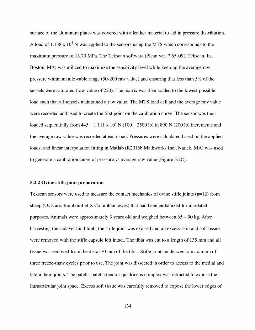
134

surface of the aluminum plates was covered with a leather material to aid in pressure distribution.

A load of 1.138 x 104 N was applied to the sensors using the MTS which corresponds to the

maximum pressure of 13.79 MPa. The Tekscan software (iScan ver. 7.65-09I, Tekscan, In.,

Boston, MA) was utilized to maximize the sensitivity level while keeping the average raw

pressure within an allowable range (50-200 raw value) and ensuring that less than 5% of the

sensels were saturated (raw value of 220). The matrix was then loaded to the lowest possible

load such that all sensels maintained a raw value. The MTS load cell and the average raw value

were recorded and used to create the first point on the calibration curve. The sensor was then

loaded sequentially from 445 – 1.111 x 104 N (100 – 2500 lb) in 890 N (200 lb) increments and

the average raw value was recorded at each load. Pressures were calculated based on the applied

loads, and linear interpolation fitting in Matlab (R2016b Mathworks Inc., Natick, MA) was used

to generate a calibration curve of pressure vs average raw value (Figure 5.2C).

5.2.2 Ovine stifle joint preparation

Tekscan sensors were used to measure the contact mechanics of ovine stifle joints (n=12) from

sheep (Ovis aris Rambouillet X Columbian ewes) that had been euthanized for unrelated

purposes. Animals were approximately 3 years old and weighed between 65 – 90 kg. After

harvesting the cadaver hind limb, the stifle joint was excised and all excess skin and soft tissue

were removed with the stifle capsule left intact. The tibia was cut to a length of 135 mm and all

tissue was removed from the distal 70 mm of the tibia. Stifle joints underwent a maximum of

three freeze-thaw cycles prior to use. The joint was dissected in order to access to the medial and

lateral hemijoints. The patella-patella tendon-quadriceps complex was retracted to expose the

intraarticular joint space. Excess soft tissue was carefully removed to expose the lower edges of

135

the medial and lateral menisci. All major ligaments were left intact aside from the long digital

extensor tendon which was sectioned at the femoral insertion and removed. Two horizontal holes

were drilled through the femur to aid in positioning during mechanical testing. First, with the

femur held at approximately 60º of flexion, a 10.5 mm hole was drilled through the femoral

condyles just above the femoral attachment of the lateral collateral ligament, parallel with the

tibial plateau. A second 10.5 mm hole was drilled through the femoral shaft 75 mm proximal to

the first hole. The distal tibia was potted in resin (Smooth-Cast 321) in a cylindrical cardboard

mold with a diameter of 50 mm and a length of 70 mm.

Fishing line was used to insert Tekscan sensors in an anterior-to-posterior direction under the

menisci on the tibial plateau such that one prong of a sensor was in the medial hemijoint and the

other prong was in the lateral hemijoint. Each sensor was covered with clear tape to prevent

contact with fluids during testing.

5.2.3 Ovine stifle joint mechanical testing

The MTS was equipped with an 8890 N load cell (Interface 1210AF-2k, Scottsdale, AZ) and

used to apply compressive loads to the stifle joint at fixed flexion angles. Three testing

conditions were assessed consecutively for each joint: ACL intact (Figure 5.3A), ACL transected

(Figure 5.3B), and either a soft tissue allograft (n=6, Figure 5.3C) or an electrospun scaffold

ACL reconstruction (n=6, Figure 5.3D), described below. A custom-built load frame was able to

fix the stifle joint in flexion angles from 0-90º in 7.5º increments (Figure 5.4). The femur was

held in the upper loading frame with two rods. The tibia was secured in a steel cup attached to a

locking universal joint which allowed for control of tibial varus/valgus and internal/external

136

rotations. The universal joint could be moved laterally to ensure no excessive varus/valgus

rotation and for each joint, the lateral position was recorded and maintained across all testing

conditions. The amount of internal/external rotation was recorded for each flexion angle of each

joint and then maintained for that joint and angle across all testing conditions. The patella-patella

tendon-quadriceps complex was tensioned with a 5 kg weight to keep the complex taut.

Figure 5.3: Ovine cadaver stifle joint test conditions: ACL intact (A), ACL transected (B) implanted soft tissue graft (C), and electrospun scaffold implanted (D).

137

Three fixed flexion angles were assessed: 45º, 60º, and 75º flexion which mimics flexion angles

of the ovine stifle joint during normal gait30. The MTS was used to apply a compressive force in

222 N (50 lb) increments from 222 – 1778 N (50 – 400 lb), at each flexion angle which

corresponds to the approximate force experienced on the ovine tibial plateau during gait.

Tekscan sensor raw value readings were recorded for the medial and lateral hemijoint at each

load and flexion angle. A custom Matlab code was used to generate pressure maps and calculate

mean and peak contact pressures and contact areas based on the Teskcan sensor readings.

Figure 5.4: Ovine cadaver stifle joint testing setup front view (A) and side view (B).

138

5.2.4 Electrospun scaffold fabrication

Scaffolds were fabricated from sheets of polycaprolactone (PCL) nanofibers which were

electrospun using a previously described technique28. Briefly, a 10% w/v solution of PCL

(MW=80,000; Sigma 440744, St. Louis, MO) was dissolved in a 3:1 v/v mixture of chloroform

and methanol. A negatively charged aluminum drum rotating at a linear velocity of

approximately 12 m/s served as the collector surface to create sheets of aligned PCL nanofibers.

Nanofibers were used to create nanofiber bundles by excising a rectangular portion of a flat sheet

(approximately 5 x 175 mm) and rolling it up tightly into a cylinder28. Resulting nanofiber

bundles were approximately 0.5 mm in diameter and 175 mm in length with nanofibers primarily

aligned along the longitudinal axis.

Nanofiber bundles were secured together using a solvent casting technique to create a complete

ACL scaffold (Figure 5.1A). First, approximately 50 nanofiber bundles were cut to 35 mm in

length and tied together with sutures such that the overall diameter was approximately 4 mm. A

70% w/v PCL (Mw=50,000; Perstorp Capa 6506, Malmo, Sweden) solution was created by

dissolving 3.5 mg PCL in 5 ml dichloromethane (Fisher Chemical D37-1) in an airtight glass

container with 12 hours of rotation. 850 mL of the PCL solution was then cast into a segment of

silicone tubing and after solvent evaporation, the resulting PCL block was 6 mm in diameter and

30 mm in length. The upper half of the PCL block contained numerous voids due to the presence

of bubbles during solvent evaporation and was thus cut off and discarded. The remaining PCL

block was then inserted into a segment of silicone tubing 20 mm in length with an inner diameter

of 6 mm such that the base of the PCL block was flush with the base of silicone tubing. 140 mL

of 70% PCL solution was cast into the open space at the top of the silicone tubing and one end of

139

the nanofiber bundles was inserted into the solution. After allowing the solvent to evaporate

overnight, the procedure was repeated on the other end of the nanofiber bundles. This procedure

resulted in a scaffold with a PCL fiber region 4 mm in diameter and 20 mm in length, which

mimics the length of the native ovine ACL. Each end of the scaffold fiber region was held

together with PCL blocks 6 mm in diameter and 20 mm in length which are able to be inserted

into bone tunnels.

5.2.5 Surgical technique

ACL reconstructions were conducted by implanting either a soft tissue allograft (n=6) or an

electrospun scaffold (n=6) in place of the native ACL. Six lateral digital extensor (LDE) tendons

were harvested from the hind limbs of sheep that had been euthanized for unrelated purpose. The

LDE tendon was isolated at the junction of the metatarsal and a tendon stripper was used

proximally to remove the tendon. Harvested grafts were doubled resulting in a free soft tissue

graft approximately 6 mm in diameter and approximately 120 mm in length (Figure 5.1B). Each

graft end was augmented with sutures (Covidien, Polysorb 2-0) and grafts were kept hydrated

with phosphate buffered saline (PBS) solution until use.

All remnant ACL tissue was removed to enable visualization of the tibial and femoral ACL

footprints. With the stifle joint held at approximately 110º of flexion, a femoral bone tunnel was

created originating at the femoral footprint of the ACL. A 2.4 mm guide wire (Arthrex AR-

1250SB) was drilled through the femur and then a 7 mm “inside-out tunnel” was drilled over the

guide wire with an acorn reamer (Arthrex AR-1407-LP). The entire femoral bone tunnel was

approximately 30 mm in length. Care was taken to avoid disrupting the PCL and any other

ligaments. A tibial drill guide was used to create a tibial bone tunnel with a similar technique.

140

Care was taken to damage surrounding soft tissue during. A notch was created on the anterior

margin of the femoral and tibial bone tunnels and each tunnel was tapped with a 7 mm tap.

For implantation of the soft tissue allograft, a passing pin was used to pull the distal end of the

graft into the femoral tunnel inside-out. The graft was tensioned on the posterio-lateral aspect of

the femoral tunnel and a 7 mm stainless steel interference screw (Arthrex AR-1370H-25) was

inserted “inside-out” into the posterior-medial aspect of the femoral tunnel. A passing pin was

used to pull the free end of the graft into the tibial tunnel. Care was taken to ensure that there was

no twisting of the graft within the joint space. The graft was tensioned along the posterio-lateral

aspect of the tibial tunnel and a 7 mm stainless steel interference screw was inserted “inside-out”

into the antero-medial aspect of the tunnel.

For implantation of the electrospun scaffold, 3 mm holes were drilled in the ends of the PCL

blocks and fishing line was inserted through the holes to serve as passing sutures. A passing pin

was inserted first through the tibial bone tunnel and the scaffold was drawn into the joint space

“outside-in” such that one PCL block remained in the tibial bone tunnel. The passing pin was

then inserted through the femoral bone tunnel and used to draw the other PCL block “inside-out”

into the femoral bone tunnel. Care was taken to ensure that the PCL fibers were not twisted in

the joint space. While tensioning the scaffold via the tibial passing sutures and with the joint in

high flexion, a 6 mm stainless steel interference screw (Arthrex AR-1360E) was inserted “inside-

out” into the antero-medial aspect of the femoral bone tunnel. A 6 mm stainless steel interference

screw was then inserted “inside-out” into the antero-medial aspect of the tibial tunnel.

141

5.2.6 Statistics

Data analysis was performed using Minitab (Minitab, Inc., State College, PA). Statistical

significance was assessed for each combination of load and flexion angle for mean contact

pressure, peak contact pressure, and contact area. For comparisons of mean and peak contact

pressure and contact area between ACL and ACLX conditions, all samples were grouped (max

n=12) and comparisons were made with a two-way repeated measures analysis of variance

(ANOVA) model with Tukey’s post-hoc test. Comparisons were also made between ACL,

ACLX, and scaffold conditions (max n=6) and ACL, ACLX, and graft conditions (max n=6)

using a multi-way repeated measures ANOVA with Tukey’s post-hoc test. All measures of mean

and peak contact area and contact pressure after scaffold or graft implantation were normalized

to the corresponding control (ACL intact) value to make comparisons directly between the

scaffold and graft groups. Means of scaffold and graft groups (max n=6) after normalization

were compared using two-sample t-tests. Differences corresponding to a p-value of less than

0.05 were considered to be statistically significant. Data are presented as mean ± standard

deviation.

5.3 Results

Not all stifle joints were able to withstand the higher load testing conditions due to instability

that occurred because of the extensive joint dissection necessary for Tekscan sensor insertion.

Based on a post-hoc power analysis, groups had to contain a minimum of 3 samples to achieve a

power of 0.90. Thus, the higher load testing conditions (1334 N, 1556 N and 1778 N or 300 lb,

350 lb, and 400 lb respectively) were not included in the statistical analysis (Table 5.1).

142

First examining only the ACL intact condition, the mean pressure tended to increase with

increasing load application up to a maximum mean pressure of approximately 1.5 MPa in the

medial hemijoint and 1 MPa in the lateral hemijoint (Figure 5.5 and Figure 5.6A). Similarly,

peak pressure increased with increasing load application up to a maximum peak pressure of

approximately 4 MPa in the medial hemijoint and 2.5 MPa in the lateral hemijoint (Figure 5.6B).

When the ACL was intact the contact area remained generally consistent with increasing load

application, with a contact area in the medial hemijoint of approximately 250 mm2 and a contact

area in lateral hemijoint of approximately 150 mm2 (Figure 5.6C). No differences were observed

between the three different flexion angles and thus for the remaining results, the 60º flexion

angle is presented as a representative case. Statistical comparisons were also assessed for contact

parameters at all other angles (contact area: Table 5.2, mean contact pressure: Table 5.3, peak

contact pressure: table 5.4).

Table 5.1: Sample numbers for ACL-ACLX, scaffold, and graft group

143

Figure 5.5 Representative pressure maps from ACL and ACLX conditions at 60º flexion.

144

Figure 5.6: ACL intact measures of mean contact pressure (A), peak contact pressure (B), and contact area (C).

145

Table 5.2: Contact area measurements. * Indicates significant different from ACL intact at p<0.05. ^ Indicates significant difference from ACLX at p<0.05.

146

Table 5.3: Mean contact pressure measurements. * Indicates significant different from ACL intact at p<0.05. ^ Indicates significant difference from ACLX at p<0.05.

147

Table 5.4: Peak contact pressure measurements. * Indicates significant different from ACL intact at p<0.05. ^ Indicates significant difference from ACLX at p<0.05.

148

After ACL transection, medial contact pressures (mean and peak) increased significantly at all

applied loads (Figure 5.5 and Figure 5.7A). The mean and peak pressures in the ACL-deficient

joint were approximately 1.5 and 3 times higher, respectively, than the mean and peak pressures

in the ACL intact joint. Contact area in the ACL-deficient medial hemijoint significantly

decreased at all applied loads and was approximately 0.6 times the contact area of the ACL intact

joint (Figure 5.7A). In lateral hemijoint after ACL transection, significant changes were only

observed in the contact area, which significantly decreased at all loading conditions and was

roughly 0.3 times the contact area of the intact joint (Figure 5.7B).

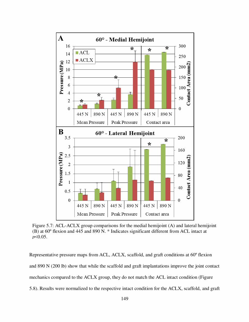
149

Representative pressure maps from ACL, ACLX, scaffold, and graft conditions at 60º flexion

and 890 N (200 lb) show that while the scaffold and graft implantations improve the joint contact

mechanics compared to the ACLX group, they do not match the ACL intact condition (Figure

5.8). Results were normalized to the respective intact condition for the ACLX, scaffold, and graft

Figure 5.7: ACL-ACLX group comparisons for the medial hemijoint (A) and lateral hemijoint (B) at 60º flexion and 445 and 890 N. * Indicates significant different from ACL intact at p<0.05.

150

implantation groups (Figure 5.9, note: conditions normalized to intact ACL such that intact ACL

=1). Contact pressures and area were not significantly different between the scaffold and graft

groups for any applied load or flexion angle (Figure 5.9A, 5.9B).

Figure 5.8 Representative pressure maps from ACL, ACL, scaffold, and graft conditions at 60º flexion and 890 N.

151

Figure 5.9: ACLX, scaffold and graft results for the medial hemijoint (A) and lateral hemijoint (B) at 60º flexion and 445 and 890 N. Values are normalized to the respective intact condition such that intact ACL = 1. * Indicates significant different from ACL intact at p<0.05. ^ Indicates significant difference from ACLX at p<0.05.

152

Comparisons are presented below wherein first we compared the scaffold and graft replacements

to the intact ACL condition, and then secondly compared the replacements to the ACLX

condition. Medial and lateral mean pressures were not different from the ACL-intact condition

after both scaffold and graft replacement at any load (Figure 5.9A, 5.9B). Peak pressure in the

medial hemijoint was however significantly greater after graft and scaffold at the higher applied

loads (>=889 N) (Figure 5.9A). At all applied loads, medial and lateral contact area was

significantly lower than the ACL-intact condition after both scaffold and graft replacement

(Figure 5.9A, 5.9B). At lower loads (<667 N) the medial mean and peak pressures with the

scaffold implanted were significantly lower than the ACL-deficient joint (Figure 5.9A).

Surprisingly, implantation of the “gold-standard” graft did not significantly improve the contact

pressures compared to the ACL-deficient joint (Figure 5.9A). Regardless of scaffold or graft

implantation, contact area in the medial and lateral hemijoints was not significantly different than

the ACL-deficient joint (Figure 5.9A, 5.9B).

5.4 Discussion

In the present study, we assessed the ability of a novel hierarchical electrospun scaffold to restore

contact mechanics when implanted in place of the native ovine ACL. At low loads, implantation

of the scaffold lowered medial mean and peak contact pressures from levels observed in the

ACL-deficient knee. At all loads, medial mean pressure after scaffold implantation was not

different from medial mean pressure in the ACL-intact knee. This suggests that scaffold

implantation is able to normalize medial mean contact pressure and mitigate changes caused by

ACL transection. Scaffold implantation was also able to normalize medial peak pressures at

lower loads. However, at loads above approximately 890 N, the peak pressure remained

153

significantly higher than the ACL-intact peak pressure. Additionally, the point of highest

pressure was shifted posteriorly on the medial tibial plateau, similar to what was observed in the

ACL-deficient joint. Although the scaffold was not able to normalize contact pressures over the

entire range of applied loads, its ability to mitigate some changes caused by ACL transection at

low loads suggests it may be able to serve as a functional replacement.

Implantation of the scaffold was not able to restore normal tibiofemoral contact area in the

medial or lateral hemijoint. Contact area after scaffold implantation remained significantly lower

than contact area in the ACL-intact knee. Higher peak pressures distributed over a lower contact

area could result in long-term degradation of cartilage and damage to subchondral bone and

meniscal tissue19,20. However, there was a trend for implantation of the scaffold to bring the

contact areas slightly closer to intact levels suggesting that the scaffold may offer a slight

improvement from the ACL-deficient joint.

Changes in contact mechanics caused by implantation of the electrospun scaffold were compared

to changes caused by implantation of a soft tissue graft. The soft tissue graft investigated

represents a gold standard clinical ACL repair technique. Both repairs were implanted using

similar surgical techniques and were fixed in the joint with stainless steel interference screws. At

all loads and flexion angles normalized mean and peak contact pressures and contact areas were

not different with the scaffold or graft implanted. Thus, at a time-zero time point (immediately

after surgical implantation) the scaffold and graft are functionally equivalent in their ability to

restore stifle joint contact mechanics. This suggests that the scaffold may serve as a novel

alternative ACL reconstruction material that serves a similar mechanical function.

154

The inability of the scaffold to completely restore normal tibiofemoral contact pressures and

areas may be due to the scaffold mechanical properties. We have previously shown that the

modulus of the scaffold subcomponents is approximately 154 MPa which is comparable to the

160 MPa modulus of the native ovine ACL, making the scaffold a suitable potential

replacement28. However, in the toe region of the load-displacement curve the stiffness of the

implanted scaffold is approximately 8 N/mm which is only 20% of the toe region stiffness of

native ovine ACL. When load is applied to the ovine stifle joint the scaffold is loaded in tension

as it functions to restrict anterior translations of the tibia relative to the femur. The lower

stiffness may mean that the scaffold is not able to stabilize the joint since a less stiff material

experiences more deformation under applied loads. This would also explain why the scaffold

was less effective at restoring pressures at higher loads since under high loads the scaffold

experiences greater deformations and is less able to restrict tibial translation. Additionally the

surgical implantation procedure, particularly the drilling of the tibial and femoral bone tunnels,

may have damaged the articular cartilage and the medial anterior meniscal attachment, which

could account for some of the altered contact area. In future work, the surgical procedure should

be optimized to minimize damage to surrounding tissues while still enabling a secure

implantation.

Although the scaffold does not completely restore contact mechanics immediately after

implantation it is likely that the scaffold will stiffen and strengthen as it remodels in vivo. Bone

marrow-derived stem cells deposited collagen on the scaffold surface when it was maintained in

vitro for a three-week time period29. It is hypothesized that at longer time points in vivo collagen

deposition and remodeling throughout the scaffold would result in increased stiffness,

155

particularly in the toe region of the force-displacement curve. Previous groups have similarly

shown that tissue-engineered ligaments are able to stiffen and strengthen in vivo31,32. Because the

scaffold is the least effective at restoring contact pressures at high loads, a postoperative

reduction in weight bearing regime could be used to give the scaffold time to undergo

remodeling and stiffen in vivo. Future studies should assess the rate of de novo tissue deposition

and the longitudinal effect on tibiofemoral contact mechanics.

In the present study, the ovine stifle joint is used as a model for the human knee joint. The ovine

stifle joint has been previously established as an appropriate orthopedic model for the human

knee and it has been utilized for the development of ligament reconstruction techniques33–37.

Most notably for this work, the size, structure, and mechanical properties of the ovine ACL

closely match the properties of the human ACL and the contact pressures on the tibial plateau are

similar in ovine stifle joints and human knee joints15,38–40. In the present study transection of the

ovine ACL resulted in increased tibiofemoral contact pressures and decreased contact area,

which matches what has been previously observed in human ACL-deficient knees16,41. Thus the

ovine stifle joint is an appropriate model for assessing ACL reconstruction techniques and the

results obtained in the present study can likely be translated to the human knee joint.

Although the results of this work are promising there are some limitations. A significant amount

of stifle joint dissection was required to insert the Tekscan sensors, and the absence of

surrounding tissue and musculature may have affected the accuracy of results. Although contact

mechanics in the present study were measured under static uniaxial loads, in vivo loading is

dynamic and multi-directional which should be better simulated in future work. Some challenges

156

associated with the Tekscan pressure sensors may have also affected results. The Tekscan

sensors had a rectangular shape (Figure 5.1B) and did not entirely cover the tibial plateau and

thus pressures in some regions of the medial and lateral hemijoints were not recorded.

Additionally, sensor readings became saturated at high loads and sensor output may have been

affected by liquid exposure and damaged sensing elements.

Overall the results of this study suggest that our novel electrospun scaffold is a promising

material for ACL reconstructions. The scaffold restores contact mechanics just as well as a gold

standard soft tissue graft and, after remodeling time in vivo, may eventually stiffen and

strengthen to be able to further stabilize the knee joint and mitigate changes caused by ACL

deficiency.

157

REFERENCES

1. Duthon, V. B., Barea, C., Abrassart, S., Fasel, J. H., Fritschy, D. & Ménétrey, J. Anatomy of the anterior cruciate ligament. Knee Surg. Sports Traumatol. Arthrosc. 14, 204–13 (2006).

2. Butler, D., Noyes, N. & Grood, E. Ligamentous restraints to anterior drawer in the human knee : a biomechanical study. J. Bone Jt. Surg. 62, 259–270 (1980).

3. Smith, B. A., Livesay, G. A. & Woo, S. L. Biology and biomechanics of the anterior cruciate ligament. Clin. Sports Med. 12, 637–70 (1993).

4. Junkin, D., Johnson, D., Fu, F., Mark, M., Willenborn, M., Fanelli, G. & Wascher, D. in Orthop. Knowl. Updat. Sport. Med. 4 135–146 (American Academy of Orthopaedic Surgeons, 2009).

5. Levine, J. W., Kiapour, A. M., Quatman, C. E., Wordeman, S. C., Goel, V. K., Hewett, T. E. & Demetropoulos, C. K. Clinically relevant injury patterns after an anterior cruciate ligament injury provide insight into injury mechanisms. Am. J. Sports Med. 41, 385–95 (2013).

6. Vavken, P. & Murray, M. M. Treating Anterior Cruciate Ligament Tears in Skeletally Immature Patients. Arthrosc. J. Arthrosc. Relat. Surg. 27, 704–716 (2011).

7. Lohmander, L. S., Ostenberg, A., Englund, M. & Roos, H. High prevalence of knee osteoarthritis, pain, and functional limitations in female soccer players twelve years after anterior cruciate ligament injury. Arthritis Rheum. 50, 3145–52 (2004).

8. Nebelung, W. & Wuschech, H. Thirty-five years of follow-up of anterior cruciate ligament - Deficient knees in high-level athletes. Arthrosc. - J. Arthrosc. Relat. Surg. 21, 696–702 (2005).

9. Øiestad, B. E., Holm, I., Aune, A. K., Gunderson, R., Myklebust, G., Engebretsen, L., Fosdahl, M. A. & Risberg, M. A. Knee Function and Prevalence of Knee Osteoarthritis After Anterior Cruciate Ligament Reconstruction. Am. J. Sports Med. 38, 2201–2210 (2010).

10. Woo, S. L., Debski, R. E., Withrow, J. D. & Janaushek, M. A. Biomechanics of knee ligaments. Am. J. Sports Med. 27, 533–43 (1999).

11. Noyes, F., Mooar, P., Matthews, D. & Butler, D. The symptomatic anterior cruciate-deficient knee. Part I: The long-term functional disability in athletically active individuals. J. Bone Jt. Surg. 65, 154–62 (1983).

158

12. Bray, R. C. & Dandy, D. J. Meniscal lesions and chronic anterior cruciate ligament deficiency. Meniscal tears occurring before and after reconstruction. J. Bone Joint Surg.

Br. 71, 128–30 (1989).

13. Scarvell, J. M., Smith, P. N., Refshauge, K. M., Galloway, H. & Woods, K. Comparison of kinematics in the healthy and ACL injured knee using MRI. J. Biomech. 38, 255–262 (2005).

14. Imhauser, C., Mauro, C., Choi, D., Rosenberg, E., Mathew, S., Nguyen, J., Ma, Y. & Wickiewicz, T. Abnormal Tibiofemoral Contact Stress and Its Association With Altered Kinematics After Center-Center Anterior Cruciate Ligament Reconstruction: An In Vitro Study. Am. J. Sports Med. 41, 815–825 (2013).

15. Morimoto, Y., Ferretti, M., Ekdahl, M., Smolinski, P. & Fu, F. H. Tibiofemoral Joint Contact Area and Pressure After Single- and Double-Bundle Anterior Cruciate Ligament Reconstruction. Arthrosc. - J. Arthrosc. Relat. Surg. 25, 62–69 (2009).

16. Bedi, A., Chen, T., Santner, T. J., El Amin, S., Kelly, N. H., Warren, R. F. & Maher, S. a. Changes in dynamic medial tibiofemoral contact mechanics and kinematics after injury of the anterior cruciate ligament: A cadaveric model. Proc. Inst. Mech. Eng. Part H J. Eng.

Med. 227, 1027–1037 (2014).

17. Brophy, R. H., Cottrell, J., Rodeo, S. a., Wright, T. M., Warren, R. F. & Maher, S. a. Implantation of a synthetic meniscal scaffold improves joint contact mechanics in a partial meniscectomy cadaver model. J. Biomed. Mater. Res. - Part A 92, 1154–1161 (2010).

18. Cottrell, J. M., Scholten, P., Wanich, T., Warren, R. F., Wright, T. M. & Maher, S. a. A new technique to measure the dynamic contact pressures on the Tibial Plateau. J.

Biomech. 41, 2324–2329 (2008).

19. Andriacchi, T. P., Koo, S. & Scanlan, S. F. Gait mechanics influence healthy cartilage morphology and osteoarthritis of the knee. in J. Bone Jt. Surg. - Ser. A 91, 95–101 (2009).

20. Sun, H. B. Mechanical loading, cartilage degradation, and arthritis. Ann. N. Y. Acad. Sci. 1211, 37–50 (2010).

21. Biau, D. J., Tournoux, C., Katsahian, S., Schranz, P. & Nizard, R. ACL Reconstruction. Clin. Orthop. Relat. Res. 180–187 (2007).

22. Dargel, J., Gotter, M., Mader, K., Pennig, D., Koebke, J. & Schmidt-Wiethoff, R. Biomechanics of the anterior cruciate ligament and implications for surgical reconstruction. Strateg. Trauma Limb Reconstr. 2, 1–12 (2007).

23. Kiapour, A. M. & Murray, M. M. Basic science of anterior cruciate ligament injury and repair. Bone Joint Res. 3, 20–31 (2014).

159

24. Biau, D., Tournoux, C., Katsahian, S., Schranz, P. & Nizard, R. Bone-patellar tendon-bone autografts versus hamstring autografts for reconstruction of anterior cruciate ligament: meta-analysis. BMJ 332, 995–1001 (2006).

25. Krych, A. J., Jackson, J. D., Hoskin, T. L. & Dahm, D. L. A Meta-analysis of Patellar Tendon Autograft Versus Patellar Tendon Allograft in Anterior Cruciate Ligament Reconstruction. Arthrosc. J. Arthrosc. Relat. Surg. 24, 292–298 (2008).

26. Sun, K., Tian, S., Zhang, J., Xia, C., Zhang, C. & Yu, T. Anterior cruciate ligament reconstruction with BPTB autograft, irradiated versus non-irradiated allograft: A prospective randomized clinical study. Knee Surgery, Sport. Traumatol. Arthrosc. 17, 464–474 (2009).

27. Cohen, S. B. & Sekiya, J. K. Allograft Safety in Anterior Cruciate Ligament Reconstruction. Clin. Sports Med. 26, 597–605 (2007).

28. Pauly, H. M., Kelly, D. J., Popat, K. C., Trujillo, N. a, Dunne, N. J., Mccarthy, H. O. & Donahue, T. L. H. Mechanical Properties and Cellular Response of Novel Electrospun Nanofibers for Ligament Tissue Engineering : Effects of Orientation and Geometry Reference : J. Mech. Behav. Biomed. Mater. 61, 258–270 (2016).

29. Pauly, H. M., Sathy, B. N., Olvera, D., McCarthy, H. O., Kelly, D. J., Popat, K. C., Dunne, N. J. & Haut Donahue, T. L. Hierarchically Structured Electrospun Scaffolds with Chemically Conjugated Growth Factor for Ligament Tissue Engineering. Tissue Eng. Part

A 23, 823–836 (2017).

30. Tapper, J. E., Fukushima, S., Azuma, H., Sutherland, C., Marchuk, L., Thornton, G. M., Ronsky, J. L., Zernicke, R., Shrive, N. G. & Frank, C. B. Dynamic in vivo three-dimensional (3D) kinematics of the anterior cruciate ligament/medial collateral ligament transected ovine stifle joint. J. Orthop. Res. 26, 660–672 (2008).

31. Ma, J., Smietana, M. J., Kostrominova, T. Y., Wojtys, E. M., Larkin, L. M. & Arruda, E. M. Three-dimensional engineered bone-ligament-bone constructs for anterior cruciate ligament replacement. Tissue Eng. Part A 18, 103–16 (2012).

32. Leong, N. L., Kabir, N., Arshi, A., Nazemi, A., Jiang, J., Wu, B. M., Petrigliano, F. A. & McAllister, D. R. Use of ultra-high molecular weight polycaprolactone scaffolds for ACL reconstruction. J. Orthop. Res. 34, 828–835 (2016).

33. Allen, M. J., Houlton, J. E., Adams, S. B. & Rushton, N. The surgical anatomy of the stifle joint in sheep. Vet. Surg. VS Off. J. Am. Coll. Vet. Surg. 27, 596–605 (1998).

34. Proffen, B. L., McElfresh, M., Fleming, B. C. & Murray, M. M. A comparative anatomical study of the human knee and six animal species. Knee 19, 493–9 (2012).

160

35. Lu, Y., Markel, M. D., Nemke, B., Wynn, S. & Graf, B. Comparison of Single-Versus Double-Tunnel Tendon-to-Bone Healing in an Ovine Model: A Biomechanical and Histological Analysis. Am. J. Sports Med. 37, 512–517 (2009).

36. Ma, J., Goble, K., Smietana, M., Kostrominova, T., Larkin, L. & Arruda, E. M. Morphological and functional characteristics of three-dimensional engineered bone-ligament-bone constructs following implantation. J. Biomech. Eng. 131, 101017 (2009).

37. Weiler, A., Peine, R., Pashmineh-Azar, A., Abel, C., Südkamp, N. P. & Hoffmann, R. F. G. Tendon healing in a bone tunnel. Part I: Biomechanical results after biodegradable interference fit fixation in a model of anterior cruciate ligament reconstruction in sheep. Arthroscopy 18, 113–123 (2002).

38. Chandrashekar, N., Mansouri, H., Slauterbeck, J. & Hashemi, J. Sex-based differences in the tensile properties of the human anterior cruciate ligament. J. Biomech. 39, 2943–50 (2006).

39. Weiler, A., Peters, G., Mäurer, J., Unterhauser, F. N. & Südkamp, N. P. Biomechanical properties and vascularity of an anterior cruciate ligament graft can be predicted by contrast-enhanced magnetic resonance imaging. A two-year study in sheep. Am. J. Sports

Med. 29, 751–761 (2001).

40. Lee-Shee, N. K., Dickey, J. P. & Hurtig, B. Contact mechanics of the ovine stifle during simulated early stance in gait: An in vitro study using robotics. Vet. Comp. Orthop.

Traumatol. 20, 70–72 (2007).

41. Van De Velde, S. K., Bingham, J. T., Hosseini, A., Kozanek, M., DeFrate, L. E., Gill, T. J. & Li, G. Increased tibiofemoral cartilage contact deformation in patients with anterior cruciate ligament deficiency. Arthritis Rheum. 60, 3693–3702 (2009).

161

CHAPTER 6:

CONCLUSIONS AND FUTURE WORK

In summary, this work presents the development of a novel electrospun polymer scaffold for

anterior cruciate ligament (ACL) replacement. Polycaprolactone (PCL) was chosen for this

project based on its slow degradation rate and lack of harmful byproducts. The scaffold was

composed of electrospun PCL nanofibers with a size and alignment that mimics the collagen

fibers of the ACL. Sheets of aligned nanofibers were further modified into rolled nanofiber

bundles which mimic the size and structure of collagen fascicles. This hierarchical structure

likely enabled the nanofiber bundles to mimic the material properties, specifically the modulus,

of the native ACL. However the stiffness and failure loads of nanofiber bundles were still

notably lower than the collagenous components of the native ACL. Thus it may be useful to

investigate other polymers that could be used to fabricate the scaffold to improve strength and

stiffness. The mechanical properties could also be altered by modifying the diameter of

individual nanofiber bundles and increasing the packing density of the nanofiber bundles used to

compose the entire scaffold. Modifying the structure or the structure of the sub-components

would potentially increase overall scaffold strength and stiffness. Additionally, it will be

necessary to re-evaluate the mechanical properties of the scaffold after in vivo implantation since

de novo tissue deposition and polymer degradation will eventually alter mechanical properties.

In vitro, the scaffold encouraged the adhesion and proliferation of ovine bone marrow-derived

stem cells and, in combination with conjugated growth factors, promoted the deposition of

collagenous tissue. The 21-day time point investigated offers a short-term indication of in vitro

162

behavior, however, it would be valuable to conduct longer duration studies to assess long-term

tissue deposition. Any longer term in vitro studies should incorporate mechanical stimulation to

simulate in vivo loading conditions. Future work should also investigate in vitro and in vivo

degradation rate. A common challenge of tissue engineering is to balance de novo tissue

deposition with scaffold degradation to ensure degradation does happen too quickly, thus

compromising the mechanical integrity of the scaffold. If the rate of tissue deposition is not

sufficient to balance the rate of scaffold degradation it may be necessary optimize the spatial and

temporal growth factor delivery or modify the types of growth factor used in order to accelerate

de novo tissue deposition.

In order to scale up the scaffold to make it implantable in place of the ACL in the knee joint,

groups of nanofiber bundles were attached on each end with cylindrical solvent cast blocks of

PCL. The PCL blocks were designed to be inserted into bone tunnels during surgical

implantation to provide a secure fixation of the scaffold within the joint. Although other research

groups have shown that solvent cast PCL is osteoinductive and promotes bone regeneration in

tissue engineering applications, it is not known exactly how the PCL blocks will degrade and

remodel within the femoral and tibial bone tunnels. Thus, future studies assessing the in vitro and

in vivo behavior of the PCL blocks could be beneficial. Additionally, prior to clinical use, it will

be necessary to consider how to modify the manufacturing process to reduce processing times

associated with the solvent casting procedure.

Implantation of the scaffold into an ovine cadaver stifle joint was shown to be clinically feasible

however some modifications to the surgical procedure could be useful. Development of a

163

technique for determining the optimal length of the scaffold fibrous region would enable

standard tensioning of the implanted scaffolds. If the fiber region was too short the scaffold was

observed to be “tight” after implantation which could over constrain joint motion. Conversely, if

the fiber region was too long the scaffold was “loose” which could fail to constrain joint motion.

Thus it would be beneficial to decide optimal scaffold tension prior to surgery and determine

how to implement it during surgery. In the present study, the implanted scaffold was compared

to a tendon graft which was chosen as the gold standard comparison. However, a different graft

type, such as a bone-patellar tendon-bone graft, could offer a gold standard comparison that

better mimics the scaffold structure. Additionally, in the future, it would be beneficial to

investigate a variety of surgical fixation techniques including Endobutton and bioresorbable

interference screw, which have both demonstrated clinical success.

After implantation, the presence of the scaffold restored joint laxity more effectively than a gold

standard soft tissue graft ACL replacement. However the stress relaxation and pull to failure

properties of the implanted scaffold were diminished compared to the scaffold prior to

implantation. It is hypothesized that the implantation procedure may have damaged the scaffold

nanofiber bundles either by cutting through them or straining to the point of plastic deformation.

Any damage to the nanofiber bundles would diminish the ability of the scaffold to sustain

applied loads. In the future scaffold structure and surgical procedure should be modified to

ensure there is no damage to the scaffold during implantation.

Finally, the implanted scaffold was able to mitigate some changes in tibiofemoral contact

mechanics caused by ACL transection and was functionally similar to a gold standard soft tissue

164

graft. This suggests that the presence of the scaffold is able to restore contact mechanics to close

to normal levels which could prevent damage to the menisci and articular cartilage. Failure of the

scaffold to completely restore normal contact mechanics could be due to the stiffness of the

scaffold, which is significantly lower than the stiffness of the native ovine ACL. However, the

scaffold will likely undergo remodeling in vivo which could improve the strength and stiffness.

Thus since the scaffold is functionally similar to a gold standard soft tissue graft and the

mechanical properties may improve with implantation time, the scaffold may be a clinically

useful ACL replacement. Future work should assess how in vivo tissue deposition affects long-

term changes in tibiofemoral contact mechanics.

For a long-term in vivo setting, it will be important to consider the attachment of the ACL to the

underlying subchondral bone. The ligament to bone attachment occurs over an area of ~200 µm

and consists of a graded transition from the relatively compliant ligament to the stiffer

subchondral bone. This graded attachment region is vital for transmitting tensile loads applied to

the ligament to the bone and resisting mechanical failure. Typically ACL reconstruction

techniques do not attempt to recreate this complex attachment. Recapitulating the native

attachment region would enable a tissue engineered scaffold to fully replicate the structure of the

native ligament. Potentially our scaffold could be incorporated with hydrogels, bone cements,

and various cell types, to drive the in vivo formation of a graded attachment.

While the present work has demonstrated the potential of this novel hierarchical polymer

scaffold to act as a tissue engineered ACL replacement, there remains an opportunity to build

upon this knowledge for a greater future clinical impact.

165

APPENDIX A:

STANDARD OPERATING PROCEDURES

A.1 Electrospinning and Scaffold Fabrication

A.1.1 Electrospinning

Product: Random OR aligned PCL nanofiber mat Solution: 5 ml 10% solid w/w PCL solution

97:3 PCL:oleic acid, 75:25 chloroform:methanol

Item Source Location

Polycaprolactone pellets MW=80,000 Sigma 440744 Shelf over scale

Chloroform Chemistry stock room Flammables cabinet

Oleic acid TCI America O0057 Fridge

Methanol Chemistry stock room Flammables cabinet

10ml glass syringe Cadance Micro Mate Cabinet under espin setup

Luer lock 18 gauge blunt tip needle Hamilton 90134 Cabinet under espin setup

Aluminum foil Counter

Setup Components

Enclosure box

Enclosure front

Syringe pump

Voltage supply

Rotating mandrel

Rotating mandrel control box

Lab jack

Cardboard pieces

Make Polymer Solution

1. Dissolve 0.5 g PCL in 3.75 ml chloroform by taping small glass vial to the rotator.

a. Use only glass pipette to measure chloroform. Chloroform degrades plastic.

b. Wrap Parafilm around lid to ensure no evaporation.

c. Allow PCL to dissolve completely (~30min). Some small bubbles will form in dissolved

solution.

2. Dissolve 0.0152 g oleic acid in 1.25 ml methanol in small glass beaker covered with Parafilm.

a. Takes less time to dissolve, but if necessary can stir with a small stir bar.

3. When both separate solutions are completely dissolved add the oleic acid solution to the PCL

solution and stir on the stir plate until well combined (~5 min).

a. Again, always make sure to keep vial tightly capped and sealed with Parafilm

4. Solution is usable for up to ~36 hours after making

a. Wrap Parafilm around lid and store at room temperature overnight.

Setup and Procedure 1. Arrange electrospinning setup within the enclosure box as shown:

166

2. Wrap the rotating mandrel in aluminum foil, ensure there aren’t wrinkles, and secure the edges with small pieces of tape.

a. Use a new piece of tape every ~5 sheets or so, if tape wears out the foil will rip off during

spinning.

3. Carefully pour solution into glass syringe and attach needle.

a. Ensure air bubbles are not present in the syringe.

b. Depress the syringe plunger and make sure a drop of solution appears and the needle is

not blocked.

4. Turn on syringe pump and enter ejection rate of 2 ml/hr. Position syringe in the syringe pump.

5. Attach positive (red) electrode to the base of the needle and the ground (green) electrode to the

rotating mandrel collector.

6. Position the collector so that it is directly perpendicular to the needle tip 10 cm away. Make sure

that the spray ejected from the needle tip will be centered on the collector. If necessary place the

syringe pump or the collector on the adjustable lab jack or other surfaces to elevate them.

7. Hit “Run” on the syringe pump to begin ejecting the solution. Let it eject for ~30sec to make sure

it is ejecting at a steady rate. Wipe excess off tip of needle as soon as possible before starting to

spin.

8. Turn on the rotating mandrel via the control box. Adjust rotation speed to either 300 rpm (random

sheets) or 3000 rpm (aligned sheets).

9. Slide the front of the enclosure over the box. If desired black paper can be taped on the back of

the enclosure to aid in the visualization of the Taylor cone.

10. Make sure voltage supply is initially at zero, and then turn on the voltage switch on. Gradually

increase the voltage until it reaches 15 kV.

a. Voltage supply can also be switched off with the voltage set at 15 kV, but when the

voltage supply is turned back on expect the voltage to immediately be at 15 kV.

11. After ~2 min, white deposits should be visible on the aluminum foil on the rotating mandrel.

Allow solution to spin onto the rotating mandrel for 15 min depending on desired thickness of

sheet.

167

12. Turn off voltage supply and turn the voltage back down to zero. Turn off the rotating mandrel.

Open the front of the enclosure. Carefully remove foil from the rotating mandrel. Wipe excess

solution off the needle tip prior to beginning another sheet of electrospinning.

a. ALWAYS TURN OFF VOLTAGE SUPPLY BEFORE TOUCHING ANY PART OF

THE SETUP! OTHERWISE SEVERE ELECTRIC SHOCK WILL OCCUR!

Troubleshooting 1. If polymer isn’t spinning

a. Are the electrodes hooked up correctly?

i. Make sure the red lead is on the needle and the green lead is on the base of the

rotating mandrel.

b. Is the syringe pump on and running?

i. Make sure to turn it on, program the correct ejection rate, and press Run.

ii. If there was excessive arcing or sparking the pump may have shorted out. Turn it

off and back on again.

c. Is the needle clogged? (To check, try to manually push some solution out of the syringe.

It should bead up at the tip of the needle.)

i. If the needle is clogged, use a different needle and soak the clogged needle in a

beaker of chloroform (covered in Parafilm) overnight to dissolve the clog.

2. If the electrospinning looks weird on the aluminum foil

a. Was the solution made correctly?

i. Different concentrations will cause electrospinning to appear differently.

b. Are the solution components fully dissolved and fully mixed?

i. The solution should appear homogeneous within the syringe, sometimes small

bubbles are present

c. Are the spinning parameters correct?

i. 10 cm tip-to-collector distance

ii. 2 ml/hr flow rate

iii. 15 kV

3. If arcing or sparking is occurring

a. Arcing is the term for the quiet “clicking” noise that is sometimes evident when

increasing the voltage.

i. Arcing is not ideal but electrospinning can be carried out despite arcing.

ii. To decrease arcing make sure to increase the voltage very slowly.

iii. Arcing is typically more evident with increased humidity.

b. Sparking is when electric sparks can be seen between metal components of the

electrospinning setup.

i. Sparking is very dangerous. If sparking occurs turn the voltage supply off

immediately.

ii. The sparking components can be wrapped in extra electrical tape. However this

is only a temporary fix as the excessive high voltages will still be present during

spinning.

4. If globs of solution or “streamers” collect at the tip of the needle during spinning. a. This is normal with some solutions (particularly PCL) so it can be ignored unless the

excess solution is actively interfering with the spinning.

168

A.1.2 Nanofiber Bundle Fabrication

Product: Electrospun nanofiber bundles ~0.5 mm in diameter

Item Location

Sheet of electrospun nanofibers on aluminum foil Electrospinning cabinet

Scalpel Dissection tools drawer

Tweezers Dissection tools drawer

1. Lay sheet of electrospun nanofibers on flat surface

2. Beginning at one edge, gently use fingertips (wearing gloves) to begin to roll the sheet up on

itself

a. Usually works best initiate the roll at either the top or bottom edge and work towards the

other direction

b. If making aligned nanofiber bundles ensure that the direction of nanofiber alignment is

along the longitudinal axis of the nanofiber bundle

169

3. When the nanofiber bundle is ~0.5 mm in diameter use a scalpel to slice close to the rolled edge.

4. Use tweezers to pick up to pick up the nanofiber bundle and pull it away from the aluminum foil

and onto the surrounding counter. Finish rolling up the nanofiber bundle.

5. Repeat with remainder of the nanofiber sheet. If the final nanofiber bundle created with the last

edge of the electrospun sheet is far too small in diameter (i.e. if it is similar in diameter to a strand

of hair) then discard.

170

A.1.3 Electrospun Scaffold Fabrication

Product: Scaffold with dimensions:

Supply Location

Nanofiber bundles (SOP_NFB_HP) Hannah’s drawer String/suture wire Hannah’s drawer PCL (Perstorp Capa 6506) Chemical shelf

Dichloromethane (CAS 75-09-2) Flammables cabinet

Silicone tubing, 6 mm inner diameter Hannah’s drawer Dremel with thin cutoff wheel attachment

1. Gather together ~50 nanofiber bundles (each ~75 cm in length) to create a group that is ~4 mm in

diameter. Use string to tie together the nanofiber bundles in segments.

a. Each cut segment should be ~35 cm in length with suture wires tied ~7 mm from the ends

b. Guide should be used to determine placement of suture wires and cuts.

c. Usually it’s easiest to tie on each of the pieces of suture wire for entire length of the

nanofiber bundles, and then cut the segments apart.

2. Make solvent cast PCL block ~15 mm in length and ~6 mm in diameter

a. Make a 5 ml 70% PCL solution using powdered PCL

i. Dissolving 3.5 mg PCL in 5 ml of dichloromethane in a small glass vial.

ii. Dichloromethane should only be pipetted with a glass pipette.

iii. Use parafilm to seal the lid while dissolving and while not using.

20 mm PCL blocks, 6 mm in diameter

20 mm PCL nanofiber bundles, 4 mm in diameter

7 mm 7 mm

35 mm

171

iv. To dissolve, tape to rotator and allow to dissolve overnight.

b. Cast 70% PCL into a piece of silicone tubing with inner diameter of 6 mm cut to ~30 mm

in length.

i. Cover one end of the silicone tubing with a small square of aluminum foil.

ii. Use plastic transfer pipettes to pipette the dissolved PCL into the tubing.

iii. Allow to set overnight until dichloromethane has all evaporated, leaving just

solidified PCL.

iv. When all dichloromethane is used, allow glass vial to “dry” on its side overnight before removing the remaining PCL.

c. Use Dremel with thin flat cutoff wheel attachment to cut PCL block in half (to 15 mm).

1. The lower half should have significantly less bubbles; the upper half can

be discarded.

3. Attach NFBs to PCL end blocks, one end at a time

a. Insert the 15 mm PCL block into a piece of silicone tubing cut to ~20 mm in length.

i. Bottom of the PCL block should be at the bottom of the silicone tube.

ii. Similar to above, the bottom end of the tubing should be covered with a small

piece of aluminum foil.

15 mm

Top (bubbles)

Bottom

172

b. Pipette a small additional 70% PCL into the 20 mm piece of silicone tubing to fill it up to

the top.

c. Gently insert one end of a cut NFB segment into the liquid PCL.

d. Secure upright and allow it to set overnight until dichloromethane has all evaporated,

leaving just solidified PCL.

e. Repeat steps a-d to create a solid PCL block on the other end of the NFB segment.

f. Remove silicone tubing and suture wire ties.

173

A.1.4 Growth Factor Conjugation to Nanofiber Bundles

Chemical Source Product number Amount

Connective tissue growth factor Sigma-Aldrich SRP4702 20 μg

Basic fibroblastic growth factor Sigma-Aldrich F0291 25 μg

Polyallamine Sigma-Aldrich 227056 1 g (20 wt% in H20)

N,N-dimethylformamide Sigma-Aldrich 227056 100 ml

N-succinimidyl-3-maleimidoproprionate TCI America S0427 100 mg

1. Incubate fibers in a 5% solution of polyallamine with simultaneous UV radiation for 25 minutes.

2. Rinse fibers

a. Rinse 3 times in dH2O.

b. Soak in dH2O for 2 hours.

c. Rinse 3 times in dH2O.

3. Incubate fibers in a solution of 25mg N-succinimidyl-3-maleimidoproprionate in 3.3ml N,N-

dimethylformamide for 1 hour.

4. Rinse fibers

a. Rinse 3 times in dH2O.

b. Soak in dH2O for 2 hours.

c. Rinse 3 times in dH2O.

5. Incubate fibers in a 50ng/ml solution of CTGF for 2 hours.

6. Rinse fibers

a. Rinse 3 times in dH2O.

b. Soak in dH2O for 2 hours.

c. Rinse 3 times in dH2O.

Immediately after incubation characterize fibers or seed with cells

174

A.2 Cell Culture

A.2.1 General Cell Culture Media

Item Location

500ml bottle DMEM Fridge

50ml FBS aliquot Freezer

5ml pen/strep aliquot Freezer

0.5 ml amphotericin-B aliquot Freezer

60ml plastic syringe Cell culture supply drawer

0.25um filter tip Cell culture supply drawer

1. Thaw FBS, pen/strep, and amphotericin-B in water bath.

2. Discard 55ml of DMEM from the bottle.

3. If FBS and pen/strep are not already sterilized, sterile filter both into the DMEM bottle.

4. Pipette amphotericin-B into bottle.

5. Cap the bottle and mix gently by inverting.

6. Label with name and date and store in the fridge for up to 1 month.

175

A.2.2 Adipose Derived Stem Cell Culture Media

Item Location

Sterile 500ml glass bottle Middle shelf

500ml bottle ADSC DMEM Fridge

50ml FBS Freezer

5ml Pen/strep Freezer

60ml plastic syringe Cell culture supply drawer

0.25um filter tip Cell culture supply drawer

7. Thaw FBS and Pen/strep in water bath.

8. Discard 55ml of ADSC DMEM from the bottle; pour the remainder in the glass bottle.

9. Sterile filter the FBS and Pen/strep into the glass bottle.

10. Cap the glass bottle and mix gently by inverting.

11. Label and store in the fridge for up to 1 month.

176

A.2.3 Freezing Cells

Item Location

ADSC Media (warmed) Fridge

Sterile 1x PBS (warmed) Middle shelf

4ml 0.25% trypsin (per flask, warmed) Freezer

FBS for freeze media Freezer

DMSO Flammables cabinet

15ml tubes Top of incubator

20ml syringe Cell culture supplies drawer

0.25um filter tip Cell culture supplies drawer

Sterilized 2ml tubes Cell culture supplies drawer

Cryogenic storage tubes Cell culture supplies drawer

Mr. Frosty Cell culture supplies drawer

Isopropyl alcohol Flammables cabinet

1. Check with the cell culture microscope to ensure cells are ~80% confluent.

2. Aspirate media from flasks.

3. Add 13ml PBS to each flask, aspirate off.

a. Make sure to add PBS to the NON-growing side of the flasks.

b. Trypsin is inactivated by media so the PBS ensure that all media is removed before

adding the trypsin.

4. Add 1ml of trypsin to each flask, aspirate off.

5. Add remaining 3ml of trypsin to each flask, incubate for 7-10 minutes.

6. Check flasks with cell culture microscope to ensure that nearly all the cell have come unattached

from the surface of the flasks.

a. It may be necessary to gently tap the side of the flasks to release any stuck on cells.

b. If cells are NOT detached allow to incubate for another few minutes.

c. Do not incubate cells for longer than 10 minutes, the trypsin could start to kills them.

7. Add 10ml of media to each flask to inactivate the trypsin.

8. Pour the mixture of media/trypsin/cells from each flask into a 15ml tube.

9. Centrifuge the 15ml tubes at 280G for 5 minutes

10. CAREFULLY aspirate off the supernatant, making sure not to disturb the pellet.

11. Pick 1 tube of cells to count.

a. Add 1ml of PBS to the tube and gently pipette up and down to resuspend the cells.

b. Add an additional 4ml of PBS to the tube and pipette to mix.

c. Take 100ul of PBS/cell mixture from the 5ml PBS/cell mixture and pipette into a sterile

2ml tube.

d. Using the cell counter, count the number of cells in the 100ul sample.

i. Cell counter will return a count of cells/ml.

ii. Multiply the returned number by 5 to determine the total number of cells in 5mls

of PBS.

e. Centrifuge the tube that was counted at 280G for 5 minutes

f. Aspirate off supernatant.

12. Make freeze media

a. Need 1ml per tube of cells to freeze.

b. 90% FBS and 10% DMSO.

177

c. Sterile filter into a 15ml conical tube.

13. Resuspend all tubes of cells in 1ml freeze media.

14. Pipette each 1ml cell/freeze media mixture into cryogenic storage tubes and label all tubes with

type of cell, passage number, initials, and date.

15. Fill Mr. Frosty with isopropyl alcohol and plastic inserts.

16. Add vials of cells and put in -80C freezer for at least four hours.

17. Transfer to liquid nitrogen storage tank.

178

A.2.4 Plating and Expanding Frozen Cells

Item Location

Vial of frozen cells Liquid nitrogen storage tank

ADSC media (warmed) Fridge

15ml conical tube On top of incubator

50ml conical tube On top of incubator

T75 flasks Cell culture supplies cabinet

Sterile 1x PBS Middle shelf

1. Thaw 1ml vial of cells by swirling gently in water bath.

2. Fill 15ml tube with 4ml of media.

3. Gently pipette 1ml of cells into tube of media.

4. Centrifuge at 280G for 5 minutes.

5. Fill 50ml conical tube with the amount of media necessary to seed the desired number of T75

flasks (13ml per flask) MINUS 1ml

6. When centrifuge has finished, aspirate off the supernatant and re-suspend the cells in 1ml media.

7. Add the 1ml of media with cells to the 50ml conical tube with media.

a. Pipette gently up and down to mix cells in with larger volume of media.

b. If desired triturate the cells from the 50ml conical tube.

8. Pipette ~2ml PBS into each flask and agitate to ensure the entire growing surface is coated with

fluid. Aspirate off PBS.

9. Pipette 13ml of cell/media mixture into each T75 flask. Lay flak down and make sure there are no

bubbles and the entire growing surface is coated. Also make sure to vent the lid.

10. Check that cells are present in the flas by using the light microscope at 10x on the middle contrast

setting.

11. Place flasks in the incubator with lid facing the back.

179

A.2.5 Splitting Cells

Item Location

ADSC Media (warmed) Fridge

Sterile 1x PBS (warmed) Middle shelf

4ml 0.25% trypsin (per flask, warmed) Freezer

15ml tubes Top of incubator

50ml tubes Top of incubator

Sterilized 2ml tubes Cell culture supplies drawer

T75 flasks Cell culture supplies cabinet

1. Check with the cell culture microscope to ensure cells are ~80% confluent.

2. Aspirate media from flasks.

3. Add 13ml PBS to each flask, aspirate off.

a. Make sure to add PBS to the NON-growing side of the flasks.

b. Trypsin is inactivated by media so the PBS ensure that all media is removed before

adding the trypsin.

4. Add 1ml of trypsin to each flask, aspirate off.

5. Add remaining 3ml of trypsin to each flask, incubate for 7-10 minutes.

6. Check flasks with cell culture microscope to ensure that nearly all the cell have come unattached

from the surface of the flasks.

a. It may be necessary to gently tap the side of the flasks to release any stuck on cells.

b. If cells are NOT detached allow to incubate for another few minutes.

c. Do not incubate cells for longer than 10 minutes, the trypsin could start to kills them.

7. Add 10ml of media to each flask to inactivate the trypsin.

8. Pour the mixture of media/trypsin/cells from each flask into a 15ml tube.

9. Centrifuge the 15ml tubes at 280G for 5 minutes

10. CAREFULLY aspirate off the supernatant, making sure not to disturb the pellet.

11. Pick 1 tube of cells to count.

a. Add 1ml of PBS to the tube and gently pipette up and down to resuspend the cells.

b. Add an additional 4ml of PBS to the tube and pipette to mix.

c. Take 100ul of PBS/cell mixture from the 5ml PBS/cell mixture and pipette into a sterile

2ml tube.

d. Using the cell counter, count the number of cells in the 100ul sample.

i. Cell counter will return a count of cells/ml.

ii. Multiply the returned number by 5 to determine the total number of cells in 5mls

of PBS.

e. Centrifuge the tube that was counted at 280G for 5 minutes

f. Aspirate off supernatant.

12. Resuspend the cells in 1ml new media.

13. Fill a 50ml tube with the total amount of media needed to fill the desired number of flasks (13ml

per flask) MINUS the media that the cells are already suspended in.

14. Add the resuspended cell to the 50ml tube of media. Pipette up and down gently to mix.

15. Pipette ~2ml PBS into each flask, agitate to ensure that the growing surface is coated with fluid,

aspirate off PBS.

180

16. Pipette 13ml of cell & media mixture into each T75 flask, lay flask down and make sure entire

growing surface is coated, avoid bubbles, make sure lid is vented.

17. Check that cells are present by using the light microscope at 10x on the middle contrast setting.

18. Place in incubator with lid facing toward the back of the incubator.

181

A.2.6 Electrospinning Sterilization and Cell Culture

Item Location

Flat sheets of electrospinning Electrospinning cabinet, bottom shelf

8mm biopsy punch Cell culture supplies drawer

48 well plate Cell culture supplies drawer

Methanol Flammables cabinet

70% ethanol Flammables cabinet

Sterile 1x PBS Middle shelf

Cell culture media Fridge

50ml conical tube Top of incubator

Cells 2ml tube

1. Punch out flat electrospinning samples with 8mm biopsy punch. Use a cutting board under the

electrospinning to prevent the biopsy punch blade from becoming dull.

2. In the cell culture hood peel the electrospinning off the aluminum foil and transfer to wells of a

48 well plate.

3. Soak each sample in methanol (500μl per well) for 24 hours to ensure that all OLA has been leached out.

4. Soak each sample in 70% ethanol for 30 minutes.

5. Rinse each sample three times in sterile 1x PBS.

6. Expose samples to UV light for 30 minutes with lid off the 48 well plate.

7. Determine the number of cells necessary for seeding the desired number of samples.

a. Seed at a density of 10,000 cells/cm2

b. 48 well plate area = .95cm2

c. ~9500 cells in 500ul of media per well

d. Make sure to calculate for ~4-5 extra wells worth of cells to account for any cell/media

mixture that gets lost.

8. Follow procedures for splitting cells up until cell 12.

9. Aliquot out the amount of media necessary to seed the desired number of wells, subtracting the

amount that will be added with the cells.

10. Remove the necessary number of cells/media solution in order to get the desired number of cells.

11. Add the cell/media mixture to the larger volume of media, pipette up and down gently to mix.

12. Pipette 500ul of cell/media mixture at the final necessary cell count onto each sample, taking

care to keep each sample as flat as possible.

13. Do a half media change on day 4 to allow cells time to adhere to the samples.

182

A.2.7 Nanofiber Bundle Sterilization and Cell Culture

1. Prepare scaffolds and culture dish

a. Autoclave specially made plastic cell culture dish and glass petri dishes

b. Cut nanofiber bundles to 20mm in length

c. Place one scaffold in each well of cell culture dish

2. Sterilize scaffolds

a. Soak samples in methanol for 24 hours to ensure that all OLA has been leached out

b. Soak each samples in 70% ethanol for 30 minutes

c. Rinse each sample three times in sterile 1x PBS

d. Expose samples to UV light for 30 minutes

e. Store samples in DI water until ready for use

3. Determine number of necessary cells for seeding the desired number of samples

a. Seed at a density of 65,000 cells/cm2 based on the exposed bottom surface area of each

well in the culture plate

b. Single well = 0.09977 in2 = 0.64 cm2

0.7 in

0.125 in

c. ~40,000 cells in 200 µl of media per well

i. This is ~40,000 cells per scaffold (area of ~0.32cm2)

d. Make sure to account for ~4-5 extra wells work of cells to account for any cell/media

mixture lost during pipetting.

4. Seed cells on scaffolds

a. Follow previously established procedures for trypsanizing and counting cells.

b. Re-suspend cells in 1ml of cell culture media.

c. Calculate the necessary amount of cell/media solution of obtain the desired number of

cells

d. Aliquot out the amount of media necessary to seed the desired number of wells,

subtracting the amount that will be added with the cells.

e. Add the cell/media mixture to the larger volume of plain media; pipette up and down

gently to mix.

f. Pipette 200 µl of cell/media mixture at the necessary final cell count onto each scaffold.

g. Change media every other day. Monitor color change of media and change daily if

necessary.

183

A.3 Cell Culture Analysis

A.3.1 Cell Titer-Blue Assay

*** STAIN IS LIGHT SENSITIVE. PROCEDURE SHOULD BE CARRIED OUT IN THE

DARK***

Item Location

CellTiter-Blue reagent Freezer

1. Add CellTiter-Blue reagent to cells in culture, shake for 10 seconds, and incubate for 4 hours in

incubator.

a. Use 20ul of reagent to each 100ul of cell culture media

b. If possible include a control sample (no cells) and a blank (just media, no sample)

2. Shake for 10 seconds and add 100ul from each sample to a 96-well plate

a. If possible put samples in the 96-well plate in duplicate or triplicate

3. Read 96-well plate in a plate reader and record fluorescence at 560nm excitation, 590nm

emission

184

A.3.2 SEM Fixation

***DOES NOT NEED TO BE STERILE. PROCEDURE SHOULD BE CARRIED OUT IN FUME

HOOD***

Item Location

Sterile 1x PBS Counter

Sucrose Shelf

Sodium cacodylate Shelf

Millipore water Counter

Gluderaldehyde Fridge

Primary fixative (3% gluderaldehye in 0.1M sodium cacodylate &

0.1M sucrose)

Make new

Buffer solution (0.1M sodium cacodylate & 0.1M sucrose) Make new

35% ethanol Flammables cabinet

50% ethanol Flammables cabinet

70% ethanol Flammables cabinet

100% ethanol Flammables cabinet

Hexamethyl disilisone Flammables cabinet

Primary fixative and buffer solution

o Dissolve 0.68g sucrose and 0.43g sodium cacodylate in 19.4ml dH2O

o Buffer solution: 10ml of the solution

o Primary fixative: remaining solution plus 0.3ml gluderaldehyde

1. Aspirate cell culture media from samples

2. Rinse samples 2x in PBS.

3. Place the samples in following solutions for the designated times:

a. Primary fixative – 45 minutes

b. Buffer solution – 10 minutes

c. 35% ethanol – 10 minutes

d. 50% ethanol – 10 minutes

e. 70% ethanol – 10 minutes

f. 100% ethanol – 10 minutes

g. Hexamethyl disilisone – 10 minutes

4. Remove from final solution and store in desiccator until imaged

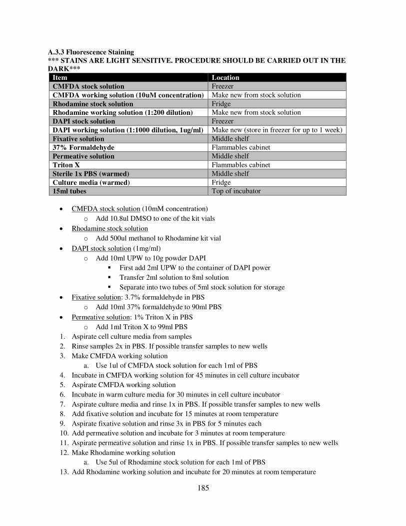
185

A.3.3 Fluorescence Staining

*** STAINS ARE LIGHT SENSITIVE. PROCEDURE SHOULD BE CARRIED OUT IN THE

DARK***

Item Location

CMFDA stock solution Freezer

CMFDA working solution (10uM concentration) Make new from stock solution

Rhodamine stock solution Fridge

Rhodamine working solution (1:200 dilution) Make new from stock solution

DAPI stock solution Freezer

DAPI working solution (1:1000 dilution, 1ug/ml) Make new (store in freezer for up to 1 week)

Fixative solution Middle shelf

37% Formaldehyde Flammables cabinet

Permeative solution Middle shelf

Triton X Flammables cabinet

Sterile 1x PBS (warmed) Middle shelf

Culture media (warmed) Fridge

15ml tubes Top of incubator

CMFDA stock solution (10mM concentration)

o Add 10.8ul DMSO to one of the kit vials

Rhodamine stock solution

o Add 500ul methanol to Rhodamine kit vial

DAPI stock solution (1mg/ml)

o Add 10ml UPW to 10g powder DAPI

First add 2ml UPW to the container of DAPI power

Transfer 2ml solution to 8ml solution

Separate into two tubes of 5ml stock solution for storage

Fixative solution: 3.7% formaldehyde in PBS

o Add 10ml 37% formaldehyde to 90ml PBS

Permeative solution: 1% Triton X in PBS

o Add 1ml Triton X to 99ml PBS

1. Aspirate cell culture media from samples

2. Rinse samples 2x in PBS. If possible transfer samples to new wells

3. Make CMFDA working solution

a. Use 1ul of CMFDA stock solution for each 1ml of PBS

4. Incubate in CMFDA working solution for 45 minutes in cell culture incubator

5. Aspirate CMFDA working solution

6. Incubate in warm culture media for 30 minutes in cell culture incubator

7. Aspirate culture media and rinse 1x in PBS. If possible transfer samples to new wells

8. Add fixative solution and incubate for 15 minutes at room temperature

9. Aspirate fixative solution and rinse 3x in PBS for 5 minutes each

10. Add permeative solution and incubate for 3 minutes at room temperature

11. Aspirate permeative solution and rinse 1x in PBS. If possible transfer samples to new wells

12. Make Rhodamine working solution

a. Use 5ul of Rhodamine stock solution for each 1ml of PBS

13. Add Rhodamine working solution and incubate for 20 minutes at room temperature

186

14. Make DAPI working solution (can keep for up to a week in the freezer, usually make ~10ml)

a. Use 1ul of DAPI stock solution for each 1ml of PBS

15. Add DAPI working solution to Rhodamine working solution and incubate for 5 minutes at room

temperature

a. Add DAPI working solution so that the final dilution of DAPI in PBS is 105:1000

(105ng/ml, 300nM)

16. Rinse 2x PBS and leave in PBS for imaging. Image ASAP

187

A.3.4 Electrospinning Histological Staining

Fixation

Item Location

Phosphate Buffered Saline (PBS) PBS Storage Tank

10% formalin Flammables cabinet

70% ethanol Flammables cabinet

Methods 1. Rinse samples in PBS.

2. Cut in half through the center.

3. Place in tubes with tops labeled 1-8L and sides labeled accordingly:

a. H.Ctrl.D1 = Histology, control, day 1

b. H.CTGF.D21 = Histology, CTGF, day 21

4. Submerge samples in 10% formalin for 24-48 hours.

5. Rinse samples 3 times with 70% ethanol.

6. Store samples in 70% ethanol at room temperature.

1L

2L

3L

4L

5L

6L

1R

2R

3R

4R

5R

6R

7L

8L

9L

10L

11L

12L

7R

8R

9R

10R

11R

12R

Histology Biochemical

assays

PCR

Cryoembedding

Item Location

Phosphate Buffered Saline (PBS) PBS Storage Tank

Sucrose Chemical shelf

Tissue Tek OCT Chemical shelf

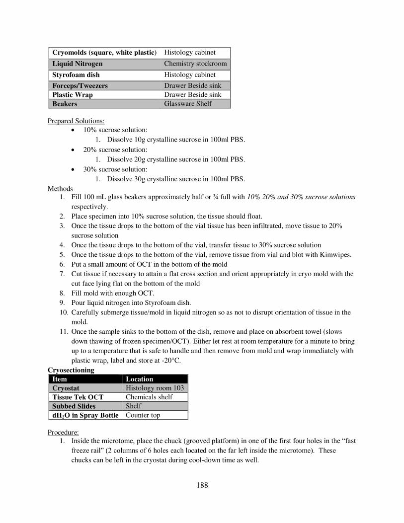
188

Cryomolds (square, white plastic) Histology cabinet

Liquid Nitrogen Chemistry stockroom

Styrofoam dish Histology cabinet

Forceps/Tweezers Drawer Beside sink

Plastic Wrap Drawer Beside sink

Beakers Glassware Shelf

Prepared Solutions:

10% sucrose solution:

1. Dissolve 10g crystalline sucrose in 100ml PBS.

20% sucrose solution:

1. Dissolve 20g crystalline sucrose in 100ml PBS.

30% sucrose solution:

1. Dissolve 30g crystalline sucrose in 100ml PBS.

Methods 1. Fill 100 mL glass beakers approximately half or ¾ full with 10% 20% and 30% sucrose solutions

respectively.

2. Place specimen into 10% sucrose solution, the tissue should float.

3. Once the tissue drops to the bottom of the vial tissue has been infiltrated, move tissue to 20%

sucrose solution

4. Once the tissue drops to the bottom of the vial, transfer tissue to 30% sucrose solution

5. Once the tissue drops to the bottom of the vial, remove tissue from vial and blot with Kimwipes.

6. Put a small amount of OCT in the bottom of the mold

7. Cut tissue if necessary to attain a flat cross section and orient appropriately in cryo mold with the

cut face lying flat on the bottom of the mold

8. Fill mold with enough OCT.

9. Pour liquid nitrogen into Styrofoam dish.

10. Carefully submerge tissue/mold in liquid nitrogen so as not to disrupt orientation of tissue in the

mold.

11. Once the sample sinks to the bottom of the dish, remove and place on absorbent towel (slows

down thawing of frozen specimen/OCT). Either let rest at room temperature for a minute to bring

up to a temperature that is safe to handle and then remove from mold and wrap immediately with

plastic wrap, label and store at -20°C.

Cryosectioning

Item Location

Cryostat Histology room 103

Tissue Tek OCT Chemicals shelf

Subbed Slides Shelf

dH2O in Spray Bottle Counter top

Procedure:

1. Inside the microtome, place the chuck (grooved platform) in one of the first four holes in the “fast freeze rail” (2 columns of 6 holes each located on the far left inside the microtome). These chucks can be left in the cryostat during cool-down time as well.

189

o `The slots are NOT numbered – make sure to label the order of your samples if you are

prepping more than one sample at a time.

2. Remove a blade from the blade container, or reuse one designated for your tissue, and grip it by

the flat edge. Raise the clamp on the right hand side of the blade holder and slide the blade in

along the left hand side of the blade holder. If it won’t go in, push gently on the bottom edge of the blade holder (the side closest to you). Push the clamp back up to lock the blade in place.

o Do not over-tighten blade

o Inspect the blade before putting it into the blade holder. Do not reuse the blade if there

are any cosmetic defects, cracks, or chips taken from the blade.

3. Wearing gloves remove the chuck and hold the post in your hand, letting it warm up slightly.

Spread embedding medium on the face of the chuck (over the grooved surface, making sure it

goes down into the grooves). NOTE: if the chuck is too cold when you put the medium on the

grooved face, the medium will not go down into the grooves. You will have to pop off the frozen

medium, wait for the chuck to warm up a bit more, and try again.

4. As soon as crystals start to appear on the outside edges of the embedding medium on the chuck

face (this will happen quickly, and the medium will turn white near the chuck), push your

embedded specimen into the center. The cutting surface (flat surface) should be exposed and

parallel with the chuck surface.

5. Allow the entire chuck/specimen combination to freeze inside the cryostat.

6. Insert the post of the chuck into the chuck holder. The small metal knob behind the chuck holder

secures the chuck in the holder, and the black lever to the right of the chuck allows the chuck to

rotate once it has been loosened.

7. Adjust the vertical position of the sample with the knob on top of chuck so that it is centered

vertically with respect to the blade. Adjust side to side alignment with knob on left side.

8. Use the retract/advance buttons on main screen of the cryostat to move chuck and holder to/away

from blade. Make sure the notch needle on the displacement wheel is up when this is done.

9. Using the handwheel on the right hand side of the cryostat, raise and lower the embedded sample

to trim through the frozen medium until you start to see the sample appear. Continue trimming

until a good cross-section appears. Adjust the angle of the chuck if the sample appears to be

cutting unevenly (i.e., if sections appear to be thicker on one side, if they appear angled, etc.).

There is no blade guard, so MAKE SURE TO BE CAREFUL TO NOT CUT YOURSELF WITH

THE BLADE when you do this.

10. Flip the “glass anti-curl plate” down so that any sections cut will slide into it underneath the glass; this will prevent sections from curling.

11. Start with 6um sections and increase to 8um if 6um does not yield good sections. Raise the glass

plate periodically to clean out any “junk sections” with the brush kept inside the microtome

12. When your first good (even thickness, longitudinal appearance) section is cut, transfer it to a

piece of slide glass by raising the anti-curl plate and pressing a piece of slide glass against the

specimen.

13. Cut at least 2 more sections that you’ll dispose of before the next section you plan to transfer to a slide (so that they’ll be separated through the depth of the core). Do not place more than 3-4

sections per slide or the cover glass will not fit. Be careful of their placement when transferring

190

to the slide glass – you won’t be able to move them once they’ve been stuck to the slide, so make sure they’re close enough together so that one coverglass will cover all 3. Obtain a total of 9

sections (2-3 per slide; 3-4 slides) per sample.

14. The remaining specimen can be refrozen by carefully melting the OCT medium from the

underside the chuck with your fingers. DO NOT let the sample melt. Refold the sample in saran

wrap and place in -20˚C non-frost free freezer.

15. Remove the blade from the cryostat; raise the blade clamp to unlock it and use forceps to gently

push along the right hand side of the blade, pushing the blade out the left side of the holder. Place

the used blade in the disposal side of the blade container.

16. Pull up the notch needle on the displacement wheel and push the “RETRACT” button to the left of the cryostat menu panel to retract the chuck and holder away from the blade holder.

17. Clean out any remaining junk by pushing it down to the side/bottom of the cryostat, but wipe out

the junk while it is frozen before turning off the cryostat for an extended period of time.

18. Lay slides on a flat surface.

19. Using a spray bottle, spray 60˚C (warm in microwave in northeast lab by liquid nitrogen tank) distilled water on slides to remove bubbles and promote the section adherence to the slide. Do not

dip slides in water or saturate the slides. Allow to dry overnight.

Troubleshooting: 1. If sectioning becomes inconsistent and slices appear shredded, one of these methods may

alleviate the problem:

a. Adjust roll plate

b. Change blade angle

c. Slice using another section of the blade

d. Flip blade over or try new blade

e. Try the sample later! – seriously it works

f. The sample may not have been embedded correctly

g. The blade may not be cold enough! Allow the cryostat to drop in temperature.

h. Try a thinner or thicker sectioning depth.

Safranin O Staining – GAGs

Item Location

Slide Holder Histology cabinet

Histology staining boxes Histology cabinet

dH2O dH2O storage tank

Tap Water Sink

Weigert’s Hematoxylin A Under fume hood

Weigert’s Hematoxylin B Under fume hood

Fast green FCFR Chemical shelf

Glacial acetic acid Under fume hood

Safranin O Chemical shelf

95% Ethanol Flammables cabinet

100% Ethanol Flammables cabinet

Xylene Flammables cabinet

Description: Stains glycosaminoglycans red, background green, cell nuclei black Prepared Solutions:

191

Weigert’s Hematoxylin (filter after use, can be used for 3 months)

1. Create 1:1 mixture Weigert’s Hematoxylin A and Weigert’s Hematoxylin B straight out of the bottle.

2. 150mL Hematoxylin A + 150mL Hematoxylin B is sufficient for 250mL slide boxes.

Fast Green FCF Solution

1. Dissolve 0.1g fast green FCFR in 1000mL dH20

1% Acetic Acid Solution

1. Mix 10mL glacial acetic acid with 990mL dH20

0.1% Safranin O Solution

1. Mix 40ml 1% Safranin O in 360 mL dH20

Procedure: 1. Place the slides in the slide holder.

2. Stain with Weigert’s iron Hematoxylin working solution for 10 minutes

3. Wash in running tap water for 10 minutes – take care not to run faucet open too far,

pressure/agitation will cause samples to come off slide

4. Stain with fast green (FGF) solution for 5 minutes

5. Rinse quickly with 1% acetic acid solution for no more than 10 – 15 seconds

6. Stain in 0.1% Safranin O solution for 10 minutes

7. Dehydrate and clear with 95% ethanol, absolute ethanol and xylene, using 2 changes each, for 2

minutes each

8. Allow to dry for ~3minutes, cover samples in Clearmount Mounting

Cleanup:

Filter Weigert’s, Safranin O and Fast green using funnel and filter paper back into their containers

Weigert’s must be placed in used container as it comes separated and is mixed to activate

Acetic acid, ethanol and xylene washes are disposed of in respective labeled waste containers.

Troubleshooting:

If slides still have stain on them, plunge slide holder up and down during the acetic acid wash and

ethanol/xylene clearings

Weigert’s solution once mixed will last approx. 3 month

Alizarin Red Staining – Calcium

Item Location

Slide holders Histology cabinet

Histology staining boxes Fume hood

dH2O dH2O storage tank

Alizarin Red Chemical shelf

Ammonium hydroxide Under fume hood

Glacial acetic acid Under fume hood

Acetone Under fume hood

Xylene Flammables cabinet

Description: Alizarin Red S, an anthraquinone derivative, may be used to identify calcium in tissue sections. The reaction is not strictly specific for calcium, since magnesium, manganese, barium, strontium, and iron may interfere, but these elements usually do not occur in sufficient concentration to interfere with the staining. Calcium forms an Alizarin Red S-calcium complex in a chelation process, and the end product is birefringent.

192

Prepared solutions:

Alizarin Red Solution:

1. Mix 2g Alizarin Red in 100mL distilled water (mix thoroughly, may take excess of 1

hour stirring to remove all clumps).

Start with 1g Alizarin Red and check particulate content. Increase to 2g Alizarin Red

if solution is transparent/ particulate content not extreme

2. Adjust pH to 4.1~4.3 with 10% Ammonium Hydroxide (only will take a few drops). The

pH is critical, so make fresh or check pH if the solution is more than one month old.

Increase pH with 10% Ammonium Hydroxide

Decrease pH with 10% Glacial Acetic Acid

Acetone-Xylene:

1. Mix equal parts acetone to xylene in the fume hood.

Procedure: 1. Stain slides with the Alizarin Red Solution for 30 seconds to 5 minutes, and observe the reaction

microscopically. Usually 2 minutes will produce nice red-orange staining of calcium.

2. Shake off excess dye and blot sections.

3. Dehydrate in acetone, 20 dips. Then in acetone-xylene solution, 20 dips. (Increase to 30 dips each

for clearer slides)

4. Clear in xylene (2 changes, 2 minutes each) and mount in a synthetic mounting medium.

Picro-sirius Red Staining – Collagen

Item Location

Slide holders Histology cabinet

Histology staining boxes Fume hood

Sirius red F3B Chemical shelf

Saturated aqueous solution of picric acid Under fume hood

Glacial acetic acid Under fume hood

Tap water Sink

Weigert’s hematoxylin A Under fume hood

Weigert’s hematoxylin B Under fume hood

Description: In bright-field microscopy collagen is red on a pale yellow background. (Nuclei, if stained, are ideally black but may often be grey or brown. The long time in picro-sirius red causes appreciable de-staining of the nuclei Prepared Solutions:

Weigert’s Hematoxylin

1. Create 1:1 mixture Weigert’s Hematoxylin A and Weigert’s Hematoxylin B

~150mL Hematoxylin A + ~150mL Hematoxylin B

2. Filter after use and can be used many times (lasts ~3 months)

Picro-sirius red solution

1. Dissolve 0.5 g Sirius red F3B in 500ml saturated aqueous solution of picric acid

2. Keeps for at least 3 years and can be reused many times

1% acetic acid

1. Mix 5ml glacial acetic acid with 495ml dH2O

Procedure 1. Place slides in a rack

193

2. Immerse the rack in solutions as defined below

Solution Time

Picro-sirius red 1 hr

1% acetic acid 30 sec

1% acetic acid 30 sec

dH2O 30 sec

dH2O 30 sec

95% ethanol 30 sec

95% ethanol 30 sec

Xylene 3 min

Xylene 3 min

3. Glue on glass coverslip with mounting medium

194

A.3.5 Electrospinning Biochemical Assays

Freezing Samples

Methods 7. Rinse samples in PBS.

8. Cut in half through the center.

9. Blot away excess liquid using a Kimwipe.

10. Place in tubes with tops labeled 5-12R and sides labeled accordingly:

a. B.Ctrl.D1 = Biochemical assay, control, day 1

b. B.CTGF.D21 = Biochemical assay, CTGF, day 21

11. Freeze in -80°C freezer

1L

2L

3L

4L

5L

6L

1R

2R

3R

4R

5R

6R

7L

8L

9L

10L

11L

12L

7R

8R

9R

10R

11R

12R

Histology Biochemical

assays

PCR

Papain Digestion of Scaffolds

Item Source Location

NaOH Sigma S8045 Chemical shelf

Na2EDTA2H2O Sigma E5134 Chemical shelf

Sodium phosphate dibasic anhydrous Sigma S3264 Chemical shelf

Sodium phosphate monobasic

anhydrous

Sigma S3139 Chemical shelf

Hydrochloric acid (HCL) Under fume hood

L-cysteine hydrochloride hydrate Sigma C7477 Chemical shelf

Papain stock solution Sigma P3125 Fridge

Prepared Solutions:

10 M NaOH (for pH adjustment of EDTA)

195

1. Add 20 g NaOH to 50ml dH2O

500mM Na2EDTA2H2O (aka EDTA)

1. Add 18.6 g Na2EDTA2H2O to 70 ml dH2O

2. pH up to 8 with 10M NaOH (~3 ml, takes 30 min-1 hr)

3. Add dH2O to make up to a final volume of 100 ml (use a graduated cylinder)

4. Autoclave and sterile filter to remove dust particles

Papain buffer extract (PBE)

1. Add 0.7098 g sodium phosphate dibasic anhydrous (Na2HPO4) and 0.5998 g sodium

phosphate monobasic anhydrous (NaH2PO4) to 90 ml dH2O

2. Add 1ml 500 mM EDTA

3. Adjust pH to 6.5 while using magnetic stirrer (~200 µl of 38% HCL)

4. Add dH2O to make up to a final volume of 100ml (use a graduated cylinder)

5. Sterile filter to remove dust particles, store at 4°C

Activated papain enzyme digest solution (APEDS)

1. Add 63 mg of L-cysteine hydrochloride hydrate to 40 ml of PBE

2. Remove papain stock solution from fridge, vortex to dissolve, swab rubber stopper with

70% ethanol

3. Remove required papain stock solution with syringe and needle and transfer to a sterile

microcentrifuge tube

4. Add 3.88 units/ml of papain stock solution to L-cysteine/PBE solution

Papain enzyme stock is 24 mg/ml and 16 units/ml 384 units/ml

3.88*1000 = 10.1 μl 384

For 40ml of activated papain enzyme digest solution

10.1 * 40 = ADD 404 µl of papain stock solution to L-cysteine/PBE

solution

Procedure 1. Remove scaffolds from storage in -80°C freezer. Excess fluid should have been previously

removed

2. Add 0.5 ml APEDS to each microcentrifuge tube to cover the sample

3. Set cell culture incubator to 0% CO2 and 50°C. Place tubes in rotator at 10 rpm and incubate

overnight or for 18 hr.

4. Vortex and shake tubes to free anything that might be trapped within the fibers

5. Remove fibers from papain solution and proceed immediately to Pico-green DNA assay to avoid

degradation.

PicoGreen DNA Content Assay

Item Source Location

Quant-iT PicoGreen dsDNA Reagent Fisher P7589 Fridge, desiccate and protect from light

20x TE buffer Fisher P7589 Chemical shelf

Lambda DNA standard Fisher P7589 Fridge, desiccate and protect from light

Prepared Solutions:

1x TE buffer (for one 96 well plate)

196

1. 1.25 ml of 20x TE stock buffer in 23.75 ml of dH2O

PicoGreen working reagent (for one 96 well plate, prepare in plastic tube)

1. Remove 55 μl from 22ml of 1x TE buffer 2. Add 55 μl of PicoGreen stock solution

3. Protect from light and use within a few hours

40 ug/ml DNA solution (for one 96 well plate)

1. Add 40 μl of DNA standard to 60 μl of 1x TE buffer

2. Vortex and briefly centrifuge

20 ug/ml DNA solution

1. Add 2 μl of DNA standard to 38 μl of 1x TE buffer

2. Vortex and briefly centrifuge

Procedure 1. Prepare DNA standards as follows:

Standard ng/well

4 x -scale

mix

Volume 2µg/ml DNA

(µl)

Volume 40µg/ml

DNA (µl)

Volume PBE to

40µl

STD0 0 0 0 40

STD1 2.5 10 5 35

STD2 5 20 10 30

STD3 10 40 20 20

STD4 50 200 5 35

STD5 100 400 10 30

STD6 150 600 15 25

STD7 200 800 20 20

2. Vortex and briefly centrifuge standards

3. Place 10 μl of each standard and sample into individual wells in triplicate in a 96 well plate

4. Add 190 μl of PicoGreen working reagent to each well (mix well)

5. Cover plate with tin foil and allow to incubate for 5 minutes in the dark at room temperature

6. Read in plate reader at 480 nm excitation and 520 nm emission.

7. Using standard curve and taking into account dilution extrapolate DNA content for each sample.

Standard Curve

Determination of GAG Content with a DMMB Assay

y = 0.5366x

R2 = 0.9965

0.000

20.000

40.000

60.000

80.000

100.000

120.000

0 50 100 150 200 250

DNA Content (ng/well)

Fluo

rese

nce

197

Item Source Location

Sodium chloride Fisher S271 Chemical shelf

Glycine Fisher G48 Chemical shelf Dimethylmethylene salt Sigma 341088 Chemical shelf

38% hydrochloric acid Under fume hood

Shark chondroitin sulfate Sigma C4384 Chemical shelf

Prepared Solutions:

DMMB dye (200 ml)

1. Add 150 ml of dH2O to a beaker

2. Add 0.468 g NaCl

3. Add 0.6 g glycine

4. Add 3.83 mg (0.00383 g) DMMB salt

5. Adjust the pH to 3.0 with 38% HCl (add 5 µl at a time)

6. Bring solution to 200 ml with dH2O

7. Filter solution through Whattman filter paper

8. Protect from light! DMMB dye solution is light sensitive. DMMB dye may be covered

in aluminum foil and stored at room temperature for approximately one month. Do not

use if the solution begins to precipitate.

GAG standard solution (200 µg/ml)

1. Add 2.0 mg (0.002 g) of shark chondroitin sulfate to 10 ml of dH2O

Procedure: 1. Prepare the GAG standards as follows:

Standard Final GAG

Concentration [µg/well]

Volume of

GAG Standard [µL]

Volume PBE

[µL]

STD0 0 0 90

STD1 0.5 7.5 82.5

STD2 1 15 75

STD3 2 30 60

STD4 3 45 45

STD5 4 60 30

STD6 5 75 15

STD7 6 90 0

2. Add 30 µl of each standard in triplicate 10 a 96 well plate

3. Add 10 µl of each sample in triplicate to a 96 well plate

4. Add 20 µl of PBE to each sample well

5. Prepare plate reader to measure the absorbance wavelength at 525 nm

6. Add 300 µl of the DMMB dye to each standard and sample well

7. Insert the plate into the plate reader and read immediately.

Standard Curve:

198

Determination of Collagen Content with a Hydroxyproline Assay

Item Source Location

Trans-4-hydroxy-L-proline Acros Organics 121780100 Chemical shelf

Hydrochloric acid (HCL) Under fume hood

Citric acid monohydrate Macron Chemicals 0627-12 Chemical shelf

Sodium acetate tryhidrate Sigma S209 Chemical shelf

Sodium hydroxide Sigma S318 Chemical shelf

Acetic acid Under fume hood

n-propanol Macron Chemicals 7169-04 Flammable cabinet

Chloramine T Sigma 857319 Chemical shelf

70% perchloric acid Sigma 244252 Chemical shelf

4-(Dimethylamino)benzaldehyde Fluka 39070 Chemical shelf

Prepared Solutions:

Hydroxyproline stock solution (1 mg/ml)

1. Add 40 mg of trans-4-hydroxy-L-proline to 40 ml of dH2O

2. Store in fridge, expires after 3 months

Citrate stock buffer (prepare 100 ml solution, use fresh batch for each experiment)

1. Add 5.04 g citric acid monohydrate to 80 ml dH2O

2. Add 11.98 g sodium acetate trihydrate

3. Add 3.4 g sodium hydroxide

4. Add 1.26 ml acetic acid

5. Adjust pH to 6.1 (use 38% HCL, takes ~100 µl)

6. Add dH2O to bring total volume to 100 ml

7. Filter with Whatman paper

8. Store in fridge

Assay buffer (prepare in 15ml tube, enough for two plates)

1. 1.5 ml n-propanol

2. 1 ml dH2O

3. 5 ml citrate stock buffer

199

Chloramine-T reagent prepare in 15 ml tube (enough for one plate)

1. Add 141 mg Chloramine T to 0.5 ml dH2O

2. Place in oven at 60C for 10 min to dissolve

3. Add 0.5 ml n-propanol

4. Add 4 ml citrate stock buffer

5. Wrap tube in tinfoil until use

DMBA reagent

1. 6 ml n-propanol

2. 3 ml 70%perchloric acid

3. 4.5 g 4-(Dimethylamino)benzaldehyde

4. Wrap tube in tinfoil until use

Procedure: 1. Sample preparation

2. Standard preparation

a. Create a 50 ug/ml hydroxyproline solution (1 in 20 dilution) from the 1 mg/ml stock

solution

i. Take 50 ul of hydroxyproline stock solution

ii. Add 950 ul PBE

iii. Vortex and briefly spin

b. Prepare standards as described below, vortex and briefly spin

Standard ID Vol 50µg/ml HYP (µl) Vol PBE to 1000µl Add 60 µl to each well (ng/well)

STD0 0 1000 0

STD1 5 995 15

STD2 20 980 60 STD3 40 960 120

STD4 70 930 210

STD5 100 900 300

STD6 125 875 375

STD7 150 850 450 TOTAL 510 μL 7490 μL

3. Assay procedure

a. Add 60 ul (in triplicate) of standards and samples to wells

b. With a multichannel pipette add:

i. 20 ul of assay buffer

ii. 40 ul of chloramine-T reagent

c. Cover the plate with tinfoil and incubate at 20 min at room temperature to allow

hydoxyproline oxidation to complete

d. Add 80 ul of DMBA reagent. Solution will become cloudy. It is essential to mix the

contents using the pipet until the solution becomes clear

e. Cover with SealPlate and incubate in an oven at 60C for 20 min

f. Cover plate with tinfoil and allow to cool for 25 min

g. Remove SealPlate carefully after cooling

h. Read in a plate reader at 570 nm. Hdryoxyproline levels in samples can be estimated

from the standard curve

200

Standard curve:

Relationship between hydroxyproline and collagen: Hydroxyproline is an amino acid that is only found in collagen and elastin. Hydroxyproline is formed via the costranslational hydroxylation of the amino acid proline. During the hydroxyproline assay the pyrrolidine ring of the hydroxyproline amino acid undergoes oxidative dehydrogenation to a pyrrole ring in the presence of 4-(dimethylamino)benzaldehyde with chloramine-T used as an oxidizing agent. Spectrophotometric analysis is then used to assess color change as an indication of the amount of hydroxyproline present. The hydroxyproline content of soluble collagen Type 1 was found to be 13%, which corresponds to a hydroxyproline-to-collagen ratio of 1:7.69. This ratio can be used to estimate the collagen content. Thus when a well of a 96 well plate is found to have 100 ng of hydroxyproline present the amount of collagen Type 1 present can be calculated to be 794 ng. Ref: Ignat'eva, N. Y., N. A. Danilov, et al. (2007). "Determination of hydroxyproline in tissues and the

evaluation of the collagen content of the tissues." J Anal Chem 62(1): 51-57.

201

A.4 Mechanical Testing

A.4.1 Electrospinning Tensile Test

Item Location

Flat sheets of electrospinning Cabinet under espin setup

Spray gun MTS cabinet

India ink Shelf over scale

Cardboard enclosure Top of fridge

Dogbone punch Hannah’s drawer Cutting board Hannah’s drawer Press Bolted to tabletop

Divided box Tupperware cabinet

Thin film grips with sandpaper Tooling cabinet

Thin film grip adapter plate and screws Tooling cabinet

Thin film grip to adapter plate adapter Tooling cabinet

2lb Futek load cell Tooling cabinet

2 and 10lb load cell adapter plate and screws Tooling cabinet

Thin film grip to load cell adapter Tooling cabinet

Flea3 camera Tooling cabinet

Preparation of samples

1. Electrospin flat sheets (see protocol on T DriveElectrospinning_HP)

2. Speckle coat sheets

a. Attach the top pin piece to the compressed air can. Make sure the pin is fully unscrewed

while attaching.

b. Connect the air cable to the sprayer and the can of compressed air.

c. Fill the bottle with India ink and attach to the sprayer. To release air screw down the pin

on the compressed air can.

d. Tape sheets of electrospinning to the cardboard enclosure and spray from ~1ft away by

depressing the button on the sprayer. It usually helps to practice first on white paper to

ensure a desirable speckle pattern. Aim for a light even coating of ink with individual

dots visible. Avoid spraying large, thick drops of ink or the electrospinning will stick to

the aluminum foil.

202

3. Cut out samples using dogbone punch

a. Tape a few sheets of paper to the cutting board to help avoid dulling the blade.

b. Place the sheet of speckle coated electrospinning on the cutting board and position the

dogbone cutter lengthwise in the center of the electrospun sheet where the

electrospinning is the thickest.

c. Three punches can usually be made from each sheet.

d. Place the samples in labeled containers, keeping track of the sheet alignment and number.

MTS Setup 1. Setup adapters to accommodate thin film grips and 2lb load cell

a. Attach thin film grip adapter plate to lower load cell

b. Attach thin film grip to adapter plate adapter. Tape sandpaper to both thin film grips.

c. Attach bottom thin film grip. Make sure that the grip face will be exactly parallel to the

direction pictures will be taken from.

203

d. Attach the 2 and 10lb load cell adapter plate to the actuator

e. Attach the 2lb load cell adapter to the load cell adapter plate and attach the load cell to

the adapter.

f. Connect the 2lb load cell to the axial force 2 cable being sure to match up the pins

correctly.

2. Turn on and warm up the MTS (see protocol on T

driveMTS_Bionic370.02Landmark_Setup_KMF

3. After the 20 minute warmup cycle attach the thin film grip to load cell adapter to the thin film

grip and the 2lb load cell.

204

4. Manually displace the actuator to the maximum negative displacement. Move the crosshead down

until the grips are very close together but NOT touching. The two grips should still be separated

by at least 10cm.

5. Switch the manual control to torsional displacement (angle controlled) and align the top grip with

the bottom grip.

6. Switch manual control back to axial displacement and move the actuator up to a working

displacement.

7. Setup the camera stand on the MTS and attach the Flea3 camera. The camera should be ~1ft away

from the thin film grips. Adjust the height of the camera stand so that the top of the lower thin

film grip is just visible at the bottom of the camera image. Note that if the camera is positioned as

shown in figure X the recording will be upside down.

8. Setup the Flycap software and Labview to run the camera triggering program (see protocol on the

T driveMTS_Camera_Triggering_BBW, Setup and Procedure steps 1-6.

Test Procedure

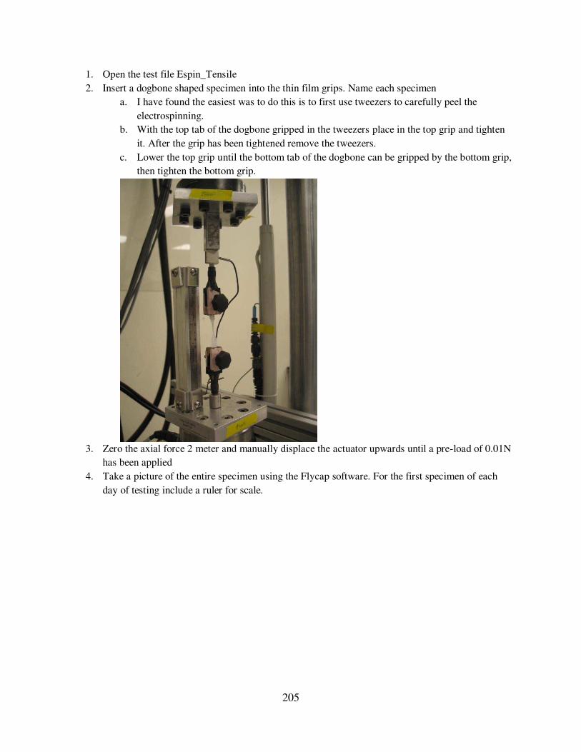
205

1. Open the test file Espin_Tensile

2. Insert a dogbone shaped specimen into the thin film grips. Name each specimen

a. I have found the easiest was to do this is to first use tweezers to carefully peel the

electrospinning.

b. With the top tab of the dogbone gripped in the tweezers place in the top grip and tighten

it. After the grip has been tightened remove the tweezers.

c. Lower the top grip until the bottom tab of the dogbone can be gripped by the bottom grip,

then tighten the bottom grip.

3. Zero the axial force 2 meter and manually displace the actuator upwards until a pre-load of 0.01N

has been applied

4. Take a picture of the entire specimen using the Flycap software. For the first specimen of each

day of testing include a ruler for scale.

206

5. In ImageJ (or FIJI) open the image and measure the gauge length of the specimen. For the first

specimen of each day of testing first set the scale using the ruler in the image. Make sure to click

“Make Global” so the same scale will be applied to all subsequent images. 6. In the MTS test file adjust displacement rate based on the gauge length and desired strain rate.

7. Continue the camera triggering procedure on step 7 of the MTS_Camera_Trigger_BBW protocol.

8. Once the specimen fails stop the test procedure as well as the Flycap recording.

9. Ensure that the specimen truly failed in the midsubstance and remove from the thin film grips.

207

A.4.2 Electrospinning Tensile Test Analysis

1. Determine the image failure number.

a. Open the images from the test in ImageJ via FileImportImage Sequence and

navigate to the file where the test images are stored. If there are a large number of images

(0.1% strain rate typically results in 8000 images) only open the final ~1000 images.

b. Scroll through the image sequence and note the first image where the specimen is no

longer intact.

2. Run the Matlab program Flat_Sheet_Espin.m to determine the true image collection rate.

a. Will ask you to input the strain rate, the gauge length, and the failure image number.

When the new ‘Choose file’ window opens click cancel to exit the program. b. Assess the resulting variable ‘dic_images’ to determine how many images to include in

the DIC analysis

i. This number is determined based on the image rate and the amount of the test

that will be analyzed. DIC analysis will be run on the first 150 seconds of testing

(0.1% strain rate), the first 15 seconds of testing (1% strain rate), the first 4

seconds of testing (5% strain rate), or the first second of testing (25% strain rate).

3. Prepare the test images for the DIC analysis program

a. Create a subfolder within the folder of test images that includes the number of images

specified in the ‘dic_images’ variable.

b. Crop these images to include only the specimen and a small portion of each grip. Make

sure that the cropped region will include the specimen for all of the images by checking

the first and last images. Save in a new subfolder.

208

i. The files in the “Cropped” subfolder should be saved sequentially starting with

the first image.

4. Run the DIC analysis program in Matlab

a. Ensure the folder with the Kevin_DIC program files has been added to the working path.

b. Open Matlab and set the directory to be the “Cropped” folder for the desired specimen. File names should be number sequentially.

c. In the Matlab terminal type “image_setup_GUI” and press Enter. Select the appropriate file extension, typically .tif. For the specimens tested at 0.01%strain/sec set the skip to

10.

d. In the Matlab terminal type “correlate_images_GUI. Set the type of loop to serial, with

the reference image set to preceding image. Choose all the other settings as shown and

click “Correlate Images”

209

e. Now a grid must be generated on the reference image. When the window appears select

the reference image (the first sequentially labeled image with no displacement). Using the

crosshairs select the area to be analyze as directed. It’s best to choose a region in center of the specimen to avoid edge effects. Also make sure the entire rectangular region of

interest is within the center rectangular area of the dogbone.

f. Enter the step size (in pixels) to 10 for the first iteration. Click “OK” and then “Keep this

grid”

210

g. All windows will close when the correlation is compute.

h. In the Matlab terminal type “visualize_data_GUI”. Select full data from the drop down menu and click “Filled Contour Plot”

i. Select the follow settings and click “View Contour plot”

j. Advance through the test images and observe the contour plot for the entire test. There

should not be any lost data points (represented by white pixels) in the final image.

211

k. Run the “correlate_images_GUI” step again keeping all settings the same except

changing the step size to 2 pixels. This will produce a finer, more accurate grid.

l. Run the “visualize_data_GUI” step again to confirm that there are still no lost data

points.

212

m. In the Matlab terminal type “compute_data_GUI” and choose the settings shown.

n. Run the “visualize_data_GUI” step again. Still select full data from the drop down menu

but now click “Spatial Average”

213

o. Use the settings shown to view the computed strains. When prompted save the resulting

strains in an Excel file.

p. This will display a graph of the percent strain the y direction as a function of image

number.

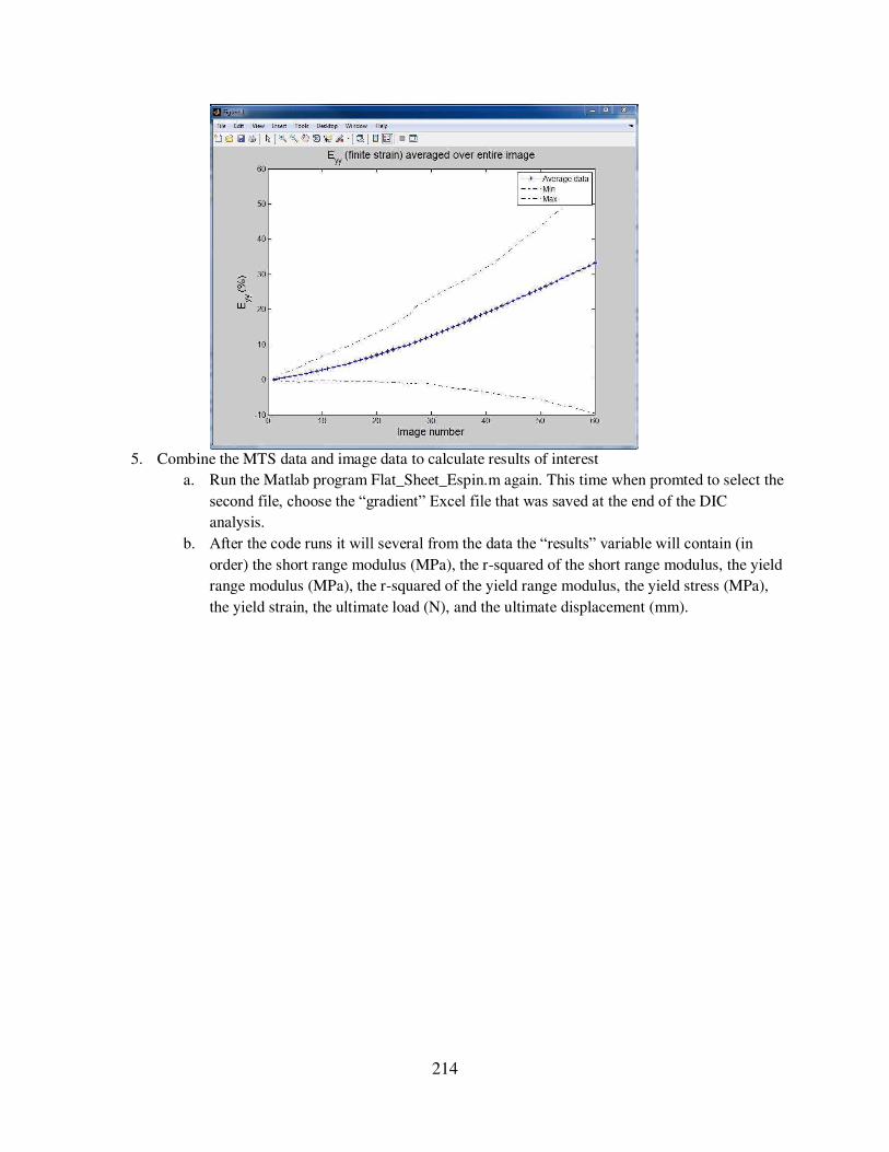
214

5. Combine the MTS data and image data to calculate results of interest

a. Run the Matlab program Flat_Sheet_Espin.m again. This time when promted to select the

second file, choose the “gradient” Excel file that was saved at the end of the DIC

analysis.

b. After the code runs it will several from the data the “results” variable will contain (in order) the short range modulus (MPa), the r-squared of the short range modulus, the yield

range modulus (MPa), the r-squared of the yield range modulus, the yield stress (MPa),

the yield strain, the ultimate load (N), and the ultimate displacement (mm).

215

216

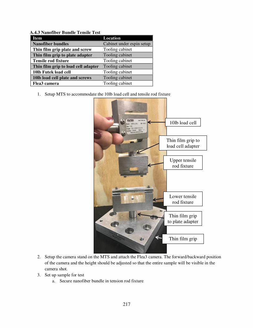
217

A.4.3 Nanofiber Bundle Tensile Test

Item Location

Nanofiber bundles Cabinet under espin setup

Thin film grip plate and screw Tooling cabinet

Thin film grip to plate adapter Tooling cabinet

Tensile rod fixture Tooling cabinet

Thin film grip to load cell adapter Tooling cabinet

10lb Futek load cell Tooling cabinet

10lb load cell plate and screws Tooling cabinet

Flea3 camera Tooling cabinet

1. Setup MTS to accommodate the 10lb load cell and tensile rod fixture

2. Setup the camera stand on the MTS and attach the Flea3 camera. The forward/backward position

of the camera and the height should be adjusted so that the entire sample will be visible in the

camera shot.

3. Set up sample for test

a. Secure nanofiber bundle in tension rod fixture

Lower tensile rod fixture

Upper tensile rod fixture

10lb load cell

Thin film grip to load cell adapter

Thin film grip to plate adapter

Thin film grip plate

218

i. Loosen screws on rod of upper fixture and insert one end of the nanofiber bundle

through the cut center of the rods. End of the nanofiber bundle should be close to

center tapped hole of the fixture.

ii. Tighten down screws on rod to sandwich the nanofiber bundle between the

halves of the rod.

iii. Wrap the nanofiber bundle around the upper half of the rod, making sure that it is

seated in the groove in the upper half of the rod to avoid stress concentrations.

iv. Lower the upper actuator down until the lower end of the nanofiber bundle is

close to the lower fixture.

v. Repeat i-iii to secure lower end of nanofiber bundle into lower fixture.

vi. The long axis nanofiber bundle should be centered on the tapped holes of the

fixture, as shown in the side-view schematic:

b. Apply a 0.1 N pre-load by manually moving the actuator upwards to ensure fixture

alignment.

c. Measure gauge length

i. After preloading take a picture of the entire specimen using the Flycap software.

For the first specimen of each day include a ruler for scale.

ii. In ImageJ (or FIJI) open the image and measure the gauge length of the

specimen. The gauge length should be measured from the center of the upper rod

Upper fixture

Lower fixture

Nanofiber

bundle

Tapped

center hole

Tapped

center hole

To plate

To load cell

219

to the center of the lower rod (points where the nanofiber bundle contacts the

rods).

iii. For the first specimen of each day of testing first set the scale using the ruler in

the image. Make sure to click “Make Global” so the same scale will be applied to all subsequent images.

iv. Gauge length should be ~15-20mm

4. Run the test

a. In the appropriate MTS test file adjust displacement rate based on the gauge length and

desired strain rate.

b. Hit run.

Gauge length

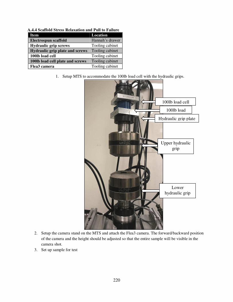
220

A.4.4 Scaffold Stress Relaxation and Pull to Failure

Item Location

Electrospun scaffold Hannah’s drawer Hydraulic grip screws Tooling cabinet

Hydraulic grip plate and screws Tooling cabinet

100lb load cell Tooling cabinet

100lb load cell plate and screws Tooling cabinet

Flea3 camera Tooling cabinet

1. Setup MTS to accommodate the 100lb load cell with the hydraulic grips.

2. Setup the camera stand on the MTS and attach the Flea3 camera. The forward/backward position

of the camera and the height should be adjusted so that the entire sample will be visible in the

camera shot.

3. Set up sample for test

Lower hydraulic grip

Upper hydraulic

grip

100lb load cell

Hydraulic grip plate

100lb load cell plate

221

a. Secure the scaffold in the hydraulic grips

i. Insert one PCL block into the upper hydraulic grip and close the grip.

1. PCL block should not be visible since it is completely within the grip.

ii. Lower the actuator until the lower PCL block drops into the lower hydraulic grip

and then close the grip.

b. Apply a 5N pre-load by manually moving the actuator upwards to ensure fixture

alignment.

c. Measure gauge length

i. After preloading take a picture of the entire specimen using the Flycap software.

For the first specimen of each day include a ruler for scale.

ii. In ImageJ (or FIJI) open the image and measure the gauge length of the

specimen. The gauge length should be measured grip to grip.

iii. For the first specimen of each day of testing first set the scale using the ruler in

the image. Make sure to click “Make Global” so the same scale will be applied to all subsequent images.

iv. Gauge length should be ~15-20mm

4. Stress relaxation test

a. Preload sample to 10N

b. Strain to 3% of gauge length at a strain rate of 2 mm/s

c. Allow to relax for 20 minutes

5. Pull to failure test

a. Preload to 5N

b. Pull to failure at a strain rate of 1%/s.

Lower hydraulic grip

Upper hydraulic grip

Gauge length

PCL block

PCL block

222

A.4.5 Ovine Stifle Anterior Drawer

1. Prepare joint

a. If knee has not been previously used:

i. Cut both bones to 135mm from the joint line. Make sure that the proximal 70mm

of the femur and the distal 70mm of the tibia are free from all soft tissue to

accommodate the cardboard tube for potting.

ii. Drill 3 wood screw into the proximal end of the femur and 3 into the distal end of

the tibia. It may be necessary to use a small drill bit to drill pilot holes.

iii. Pot femur and tibia in Smoothcast.

1. Cut a piece of cardboard tubing to 70 mm in length.

a. Outer diameter: 55 mm, inner diameter 50 mm

b. Peel layers of cardboard off the outside of the tube until it slides

easily into and out of the cup of the lower MTS fixture.

c. Cover base and sides of the tube with duct tape to ensure that

resin does not leak out.

2. Mix together equal parts of the clear and amber Smooth-Cast 321 Resin

a. Measure out each component in the sample cup with the yellow

lid, mix together in a plastic cup.

b. Stir aggressively and incorporate air.

c. Continue stirring until the mixture warms slightly and small

bubbles have formed.

3. Prop up knee so tibia hangs straight into one of the cardboard tubes.

4. When Smooth-Cast is ready (when it is slightly warm) pour into the

cardboard tubing. Leave some space at the top of the tube to allow for

expansion during hardening.

5. Allow to set until transparent and completely hardened, ~20 minutes.

6. Repeat steps 1-5 for femur.

223

iv. Dissect to a state that would enable insertion of Tekscan sensors below the

menisci.

1. Dissect back the patella/patella tendon/quadriceps complex to expose the

joint space.

2. Remove any excess tissue to expose the lower edge of the menisci, both

anteriorly and posteriorly.

3. Lateral anterior: separate the long digital extensor (LDE) ligament from

the lateral anterior meniscus by using a scalpel to gently cut underneath

the ligament.

4. Lateral posterior: remove the fat pad and dissect the muscle down from

the femoral condyle towards the tibial plateau.

5. It is necessary to sever the small attachment lateral posterior meniscal

attachments that connects to the tibial plateau. The more prominent

lateral posterior attachment connects to the femur.

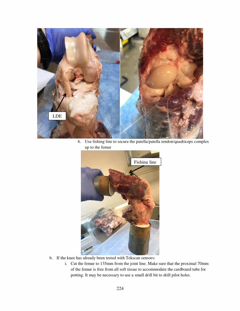
224

6. Use fishing line to secure the patella/patella tendon/quadriceps complex

up to the femur

b. If the knee has already been tested with Tekscan sensors:

i. Cut the femur to 135mm from the joint line. Make sure that the proximal 70mm

of the femur is free from all soft tissue to accommodate the cardboard tube for

potting. It may be necessary to use a small drill bit to drill pilot holes.

LDE

Fishing line

225

ii. Drill 3 wood screws into the distal femur shaft.

iii. Pot the femur in Smooth cast (see step 1.a.iii above)

iv. Use fishing line to secure the patella/patella tendon/quadriceps complex up to the

femur (see image above).

2. Prepare the MTS

a. Attach 2000 lb load cell to upper actuator

b. Turn on and warm up

c. Upper fixture: Thread cup into 2000 lb load cell

i. After cup is threaded in, zero the load cell. This only needs to be done once!

d. Lower fixture: Set up parallel cross-bars with rotating angle uniaxial fixture. Insert potted

bones into fixtures, femur in upper fixture and tibia in lower fixture.

e. Adjust the angle of the lower fixture so that the tibia is at 90º of flexion relative to the

femur.

f. Tighten down all fixtures (including the screws of the cup) and ensure that the load cell

reads zero (indicating the knee is not being tensioned or compressed).

3. Anterior drawer test

a. Open MTS program: Ovine whole knee_AD.

b. Apply a 5 N preload by manually moving the actuator upwards to ensure fixture

alignment.

c. Hit run on the MTS program.

i. Program will displace the femur upwards at a constant strain rate of 1 mm/s

2000lb load

Upper cup

Femur

Tibia

Rotating angle

uniaxial Parallel cross-bars

226

ii. When the load cell reads 50 N the displacement wills top and the program will

hold for 10 seconds.

1. Expect ~2mm of displacement if the ACL is intact or ~5mm of

displacement if the ACL is transected.

iii. Then the femur will displace downwards 10mm.

d. When complete stop the program immediately and return the load to zero so no excess

tension or compression remains on the knee.

227

A.4.6 Ovine Stifle Stress Relaxation and Pull to Failure

1. Prepare joint

a. If knee has not been previously used:

i. Cut both bones to 135mm from the joint line. Make sure that the proximal

70mm of the femur and the distal 70mm of the tibia are free from all soft

tissue to accommodate the cardboard tube for potting.

ii. Drill 3 wood screw into the proximal end of the femur and 3 into the distal

end of the tibia. It may be necessary to use a small drill bit to drill pilot

holes.

iii. Pot femur and tibia in Smoothcast.

1. Cut a piece of cardboard tubing to 70 mm in length.

a. Outer diameter: 55 mm, inner diameter 50 mm

b. Peel layers of cardboard off the outside of the tube until it

slides easily into and out of the cup of the lower MTS

fixture.

c. Cover base and sides of the tube with duct tape to ensure

that resin does not leak out.

2. Mix together equal parts of the clear and amber Smooth-Cast 321

Resin

a. Measure out each component in the sample cup with the

yellow lid, mix together in a plastic cup.

b. Stir aggressively and incorporate air.

c. Continue stirring until the mixture warms slightly and small

bubbles have formed.

3. Prop up knee so tibia hangs straight into one of the cardboard

tubes.

228

4. When Smooth-Cast is ready (when it is slightly warm) pour into

the cardboard tubing. Leave some space at the top of the tube to

allow for expansion during hardening.

5. Allow to set until transparent and completely hardened, ~20

minutes.

6. Repeat steps 1-5 for femur.

iv. Dissect knee of all tissue that connects the femur and the tibia except the

ACL.

1. Notably transect: PCL, MCL, LCL, all muscle, the lateral posterior

meniscal attachment (connects to the femur)

2. Menisci should remain intact if desired.

229

v. Determine length of the ACL (gauge length) by measuring from the

posterior view of the knee in full extension.

1. Use calibers.

2. Measure from the top of the femoral attachment to the center of the

tibial attachment.

2. Prepare the MTS

a. Attach 2000 lb load cell to upper actuator

ACL gauge

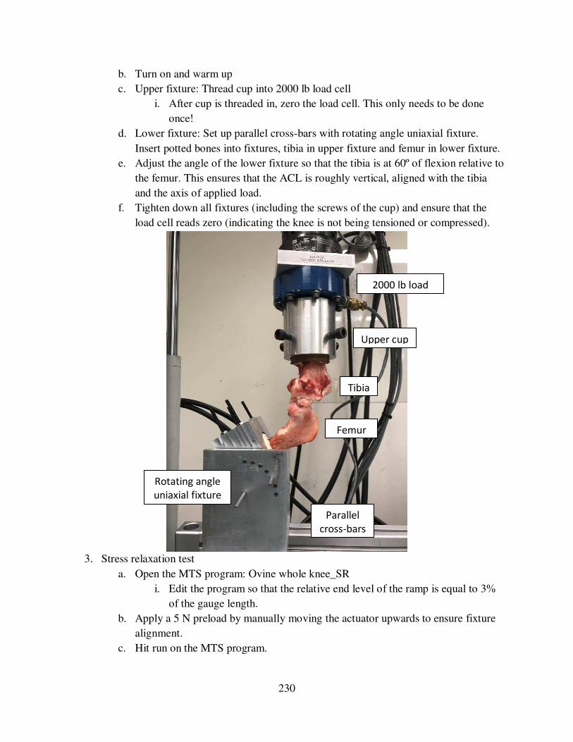
230

b. Turn on and warm up

c. Upper fixture: Thread cup into 2000 lb load cell

i. After cup is threaded in, zero the load cell. This only needs to be done

once!

d. Lower fixture: Set up parallel cross-bars with rotating angle uniaxial fixture.

Insert potted bones into fixtures, tibia in upper fixture and femur in lower fixture.

e. Adjust the angle of the lower fixture so that the tibia is at 60º of flexion relative to

the femur. This ensures that the ACL is roughly vertical, aligned with the tibia

and the axis of applied load.

f. Tighten down all fixtures (including the screws of the cup) and ensure that the

load cell reads zero (indicating the knee is not being tensioned or compressed).

3. Stress relaxation test

a. Open the MTS program: Ovine whole knee_SR

i. Edit the program so that the relative end level of the ramp is equal to 3%

of the gauge length.

b. Apply a 5 N preload by manually moving the actuator upwards to ensure fixture

alignment.

c. Hit run on the MTS program.

2000 lb load

Upper cup

Tibia

Femur

Parallel

cross-bars

Rotating angle

uniaxial fixture

231

i. Program will strain to 3% strain at a rate of 2 mm/s and hold for 20

minutes

ii. When program is complete return to zero load and wait 10 minutes

(recovery) before proceeding to pull to failure test.

4. Pull to failure test

a. Open the MTS program: Ovine whole knee_PTF

i. Edit the program so that the strain rate is 1%/s based on the gauge length

b. Hit run.

i. Program will pull to failure at a rate of 1%/s.

232

A.4.7 Tekscan Equilibration and Calibration

1. Turn on and warm up MTS.

a. Refer to SOP: MTS – Bionix Model 370.02 Landmark Setup

b. The built-in bottom load cell will be used to take readings.

2. Setup calibration fixturing as shown:

a. Use double sided tape to attach aluminum plates to the load cell and adapter.

3. Connect the Tekscan sensor to the Tekscan handle

a. Make sure the green light comes on to indicate a successful connection.

4. Initiate the Tekscan software

a. Open Iscan from the desktop.

MTS to bath plate

Extra wide

Actuator

Bottom load cell

Aluminum

plates with faux

Green light

MTS plate to bath plate

233

b. Press on sensors with your finger to make sure all the sensor rows and sensels

light up.

c. If an entire row or column of sensels is unlit, try reinserting the sensor into the

handle. If the row or column still remains out the sensor may be damaged.

5. Adjust sensitivity of Tekscan pressure sensors

a. Sandwich Tekscan sensors one on top of the other between the faux leather on the

aluminum plates.

i. Make sure that the sensors are centered (as much as possible) between the

plates

b. Load the sensor to max pressure and adjust sensitivity.

i. Load the Tekscan sensor to 2560 lbs (according to the load cell) which is

the max allowable pressure for the sensors.

ii. Click Tools Adjust sensitivity and drag the slider bar up so the

sensitivity is as high as possible without triggering one of the errors. Click

OK.

iii. Note the sensitivity value, it should be used for all subsequent tests with

the sensor.

Tekscan sensors

sandwiched between

aluminum plates

234

6. Calibrate Tekscan pressure sensors.

a. Load the Tekscan prong to the lowest load possible where all the sensels are

loaded.

i. Click Movie Snapshot (or CTRL+H) to save the raw value readings.

ii. Take note of the load (according to the load cell).

iii. Save as a .fsx file (can open only in iScan software)

1. Click File Save movie as…

2. Save the file in the subfolder “SxPy” where x corresponds to the appropriate sensor number and y corresponds to the appropriate

prong number.

3. Save as “SxPy_#” where # corresponds to the applied load. iv. Save as a .csv file (to process in Matlab or Excel)

Drag this slider bar as high as

possible without triggering an

These two metrics should have

green checkmarks, not warning signs

or errors

235

1. Click File Save ASCII… Then click OK button

2. Save the file in the subfolder “SxPy” where x corresponds to the appropriate sensor number and y corresponds to the appropriate

prong number.

3. Save as “SxPy_#” where # corresponds to the applied load. v. Click File New Recording (or CTRL+N) to start a new live session.

b. Load the Tekscan prong sequentially to 100, 300, 500, 700, 900, 1100, 1300,

1500, 1700, 1900, 2100, 2300, and 2500lbs (according to the load cell). For each

load:

i. Click Movie Snapshot (or CTRL+H) to save the raw value readings.

ii. Save as a .fsx file (can open only in iScan software)

1. Click File Save movie as…

2. Save the file in the subfolder “SxPy” where x corresponds to the appropriate sensor number and y corresponds to the appropriate

prong number.

3. Save as “SxPy_#” where # corresponds to the applied load. iii. Save as a .csv file (to process in Matlab or Excel)

1. Click File Save ASCII… Then click OK button

2. Save the file in the subfolder “SxPy” where x corresponds to the appropriate sensor number and y corresponds to the appropriate

prong number.

3. Save as “SxPy_#” where # corresponds to the applied load. iv. Click File New Recording (or CTRL+N) to start a new live session.

c. Process the .csv files using the Matlab code “Tekscan_calibration” to generate a calibration curve via linear interpolation fitting.

i. Make sure that the “Current folder” in Matlab contains all 14 .csv files. ii. Take note of the graphs produced to ensure that the fitted calibration curve

fits all points where the average raw value increases as pressure increases.

236

iii. Save the fitted calibration curve as a .mat file.

1. In the Matlab workspace there should be a file name

“calibration_fit”. 2. Select the file, right click, then click Save as.

3. Save in the subfolder “Calibration Fits”

4. Save as “SxPy” where x corresponds to the appropriate sensor

number and y corresponds to the appropriate prong number.

237

A.4.8 Ovine Stifle Joint Preparation for Tekscan

7. Thaw frozen knee overnight at room temperature or for ~3 hours with limb in bag submerged in

water.

a. Knee should already be dissected of all excess skin and soft tissue, with knee capsule

remaining intact.

b. Make sure to note whether the limb is a right or left.

i. The bulk of the calf muscle will be visible on the lateral side of the tibia.

8. Prepare tibia for potting (NOTE: This step is only necessary if the limb will later be used for a

tension test, such as stress relaxation or pull to failure).

a. Cut the tibia to ~135 mm from the joint line.

i. ~70 mm of the distal tibia should be free of all soft tissue

ii. Drill screws into distal tibia so that they extend outward from the bone.

1. May be necessary to drill a small pilot hole first.

2. Stop when the tip of the screw is in the bone marrow canal.

9. Drill fixture holes in femur. (NOTE: it is typically easier to drill the holes when the femur is

cleaned of all soft tissue, as described in Step 5).

a. Drill a 105 mm diameter hole just above the proximal attachment of the lateral collateral

ligament (LCL).

i. It may be necessary to remove some muscle tissue to expose the LCL attachment.

1. Use a permanent marker to mark the spot where the hole should be

drilled.

238

ii. Place cardboard below the limb to catch the drill bit after it goes through the

joint.

iii. Place the knee on its side and make sure it is at an angle of near full extension (as

much as possible, usually ~60º)

iv. Use a small drill bit to create a pilot hole at the marked spot, and then use

incrementally larger drill bits to enlarge the hole to its final size.

1. Approximate drill bit size order (in mm): small pilot hole, 65, 85, 105

2. Do not drill with a blue drop cloth under the limb it may get caught on

the drill.

v. The path of the hole should be parallel to the tibial plateau.

1. The edge of the tibial plateau can be felt through the capsule to serve as a

general guide.

2. To keep the tibial plateau horizontal and prevent rotation of the condyles

slightly elevate the proximal femur.

3. When the hole is large enough insert a rod to check for straightness

239

b. Drill a second 85 mm diameter hole in the proximal femur 75 mm from the first hole.

i. To guide the position of the second hole, insert the 10 mm bar through the first

hole and hang the knee in in the upper MTS fixture and use the second hole array

as a position guide.

240

ii. It may be necessary to dissect some soft tissue from the bone at the place where

the hole will be drilled.

iii. During drilling a second person should brace the limb from below (“inside” the fixture).

iv. Use a small drill bit to create a pilot hole at the marked spot and then use

incrementally larger drill bits to enlarge the hole to its final size.

1. Approximate drill bit size order (in mm): small pilot hole, 65, 85

v. The second hole should be parallel (as much as possible) to the first hole.

c. Position the knee in the upper MTS fixture to ensure the two holes enable insertion into

the fixture.

d. If the bars will not insert both insert in the fixture, it may be necessary to slightly enlarge

the second hole further

10. Pot tibia in SmoothCast

a. Cut a piece of cardboard tubing to 70 mm in length.

i. Outer diameter: 55 mm, inner diameter 50 mm

ii. Cover base and sides of the tube with duct tape to ensure that resin does not leak

out.

b. Mix together equal parts of the clear and amber Smooth-Cast 321 Resin

i. Measure out each component in the sample cup with the yellow lid, mix together

in a plastic cup.

ii. Stir aggressively and incorporate air.

iii. Continue stirring until the mixture warms slightly and small bubbles have

formed.

c. Suspend knee so that tibia hangs straight into the cardboard tubing.

241

i. Use a hole in the array that is similar to one which would be used during testing

and hang between two plastic bins.

ii. When Smooth-Cast is ready (when it is slightly warm) pour into the cardboard

tubing. Leave some space at the top of the tube to allow for expansion during

hardening.

iii. Allow to set until transparent and completely hardened, ~20 minutes.

iv. Once the Smooth-Cast is hardened peel layers of duct tape and cardboard off the

outside of the tube until it slides easily into and out of the cup of the lower MTS

fixture.

11. Dissect knee to gain access to medial and lateral hemijoints of the tibia.

a. To hold the knee during dissection it may be helpful to put the potted tibia into the lower

fixture and place the fixture on the benchtop

b. Dissect back the patella-patella tendon-quadriceps complex to expose the joint space.

Keep this structure intact as it will later be tensioned during testing.

242

c. Remove any excess tissue to expose the lower edge of the menisci, both anteriorly and

posteriorly.

i. Make sure to keep all major ligaments intact and to not damage the menisci.

ii. Lateral anterior: Cut and remove the LDE tendon.

iii. Lateral posterior: remove the fat pad and dissect the muscle down from the

femoral condyle towards the tibial plateau.

iv. It is necessary to sever the small attachment lateral posterior meniscal

attachments that connects to the tibial plateau. The more prominent lateral

posterior attachment connects to the femur.

243

12. Insert Tekscan pressure sensors

a. Insert the Tekscan pressure sensor into the medial hemijoint.

i. The sensor insertion is easiest to do when the rods are removed from the femur

and the tibia is in the universal cup which is free to rotate, making it easy to

move the joint as necessary for visualization.

ii. Thread a green needle threader through the medial hemijoint, starting from the

posterior aspect of the joint.

1. Make sure to “aim” the needle threader under the medial meniscus. 2. If necessary, when the needle threader emerges on the anterior aspect of

the joint, use curved tweezers to guide the needle under the medial

anterior attachment, so ensure that is it completely under the menisci.

LDE

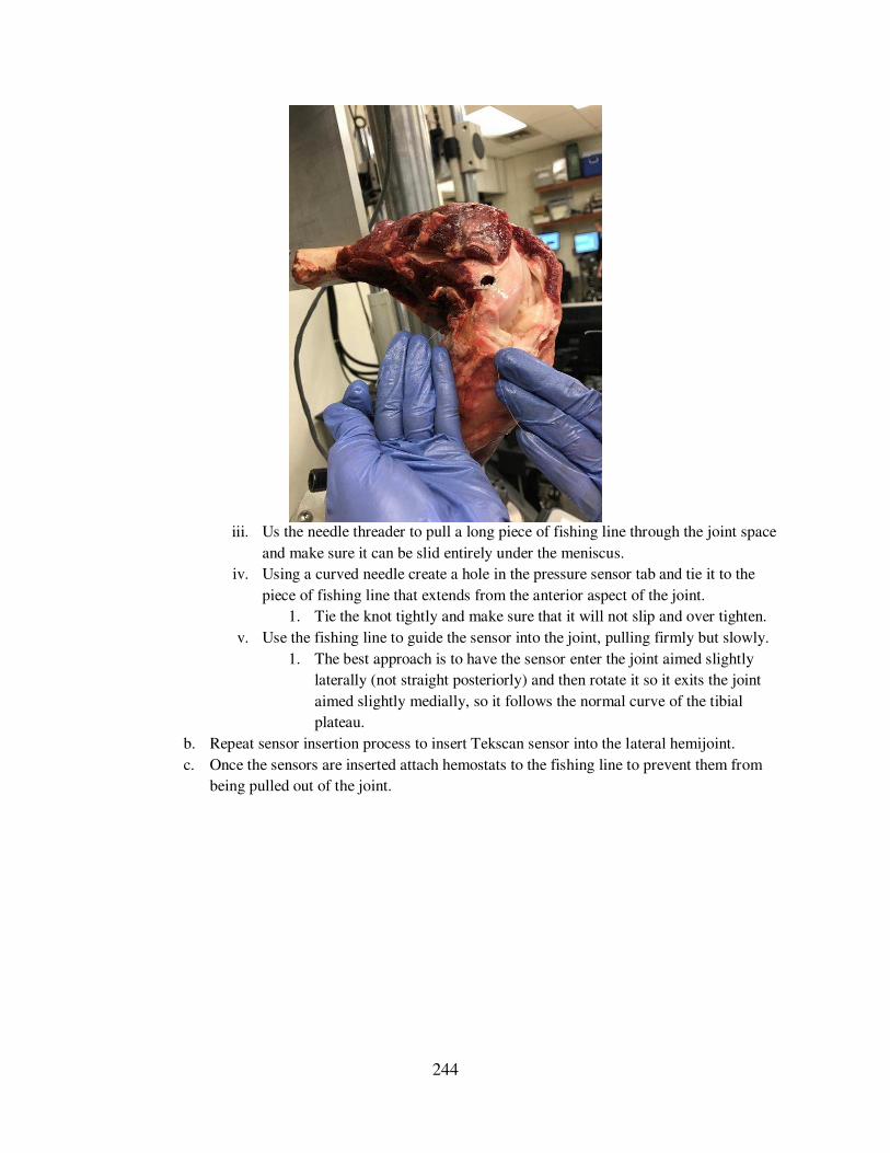
244

iii. Us the needle threader to pull a long piece of fishing line through the joint space

and make sure it can be slid entirely under the meniscus.

iv. Using a curved needle create a hole in the pressure sensor tab and tie it to the

piece of fishing line that extends from the anterior aspect of the joint.

1. Tie the knot tightly and make sure that it will not slip and over tighten.

v. Use the fishing line to guide the sensor into the joint, pulling firmly but slowly.

1. The best approach is to have the sensor enter the joint aimed slightly

laterally (not straight posteriorly) and then rotate it so it exits the joint

aimed slightly medially, so it follows the normal curve of the tibial

plateau.

b. Repeat sensor insertion process to insert Tekscan sensor into the lateral hemijoint.

c. Once the sensors are inserted attach hemostats to the fishing line to prevent them from

being pulled out of the joint.

245

Lateral

Medial

Lateral

Medial

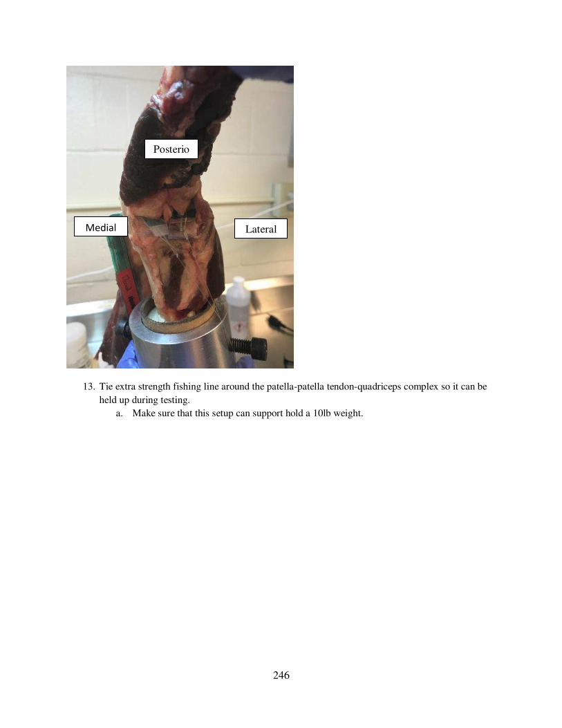
246

13. Tie extra strength fishing line around the patella-patella tendon-quadriceps complex so it can be

held up during testing.

a. Make sure that this setup can support hold a 10lb weight.

Posterior

Medial Lateral

247

A.4.9 Ovine Stifle Tekscan Testing

1. Turn on and warm up MTS

a. Refer to SOP: MTS – Bionix Model 370.02 Landmark Setup

b. Attach the 2000lb load cell to the upper actuator.

2. Set up the MTS fixturing.

a. Attach the lower universal (3 axes of rotation) cup fixture to the 8020 bars that extend

over the top of the bottom load cell.

b. Screw the threaded rod into the two pound load cell, and then screw the upper fixture

onto the other end of the threaded rod.

3. Position knee (with the Tekscan sensors in place) into the MTS fixturing

a. Remove the tibia from the lower universal cup fixture.

b. Insert the two steel rods through the holes in one side of the upper MTS fixture, then

through the femur, then through the holes on the second side of the upper MTS fixture.

i. May be necessary to rotate the fixture so the steel rods can be slid through, just

make sure to rotate straight again one positioned.

ii. This is where it is important to decide the angle of interest, and choose the array

hole accordingly.

iii. At this point, zero the load cell.

Upper fixture

Lower universal cup fixture

8020 bars

2000lbs load cell

248

c. Lower the MTS actuator and gradually lower the potted tibia into the lower universal cup

fixture.

i. Stop lowering when a small negative load is read.

d. It may be necessary to slide the plate attached to the universal cup fixture to the side to

match any natural angle of the tibia to ensure that there is no varus/valgus rotation of the

tibia.

Hole

number

Angle

(degrees)

1

15

23

4

5

6

7

8

9

14

13

12

11

10

07.515

22.5

105

97.5

90

82.5

75

60

45

30

37.5

52.5

67.5

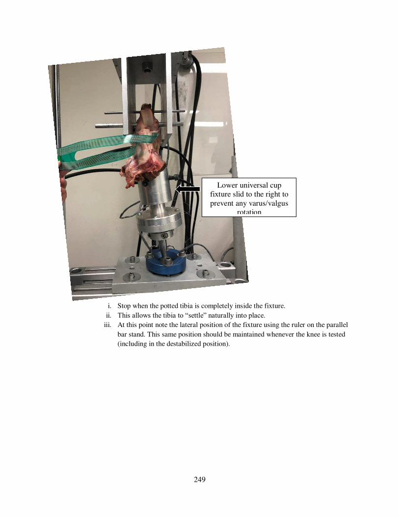
249

i. Stop when the potted tibia is completely inside the fixture.

ii. This allows the tibia to “settle” naturally into place. iii. At this point note the lateral position of the fixture using the ruler on the parallel

bar stand. This same position should be maintained whenever the knee is tested

(including in the destabilized position).

Lower universal cup fixture slid to the right to prevent any varus/valgus

rotation

250

e. Tighten down the bolts of the lower universal cup fixture to lock it into position

i. Should see a small positive force, indicative of slight tension on the joint.

ii. On the base of the universal joint make sure the center lines match, do this for

each angle.

251

iii. On the cardboard potting tube make a vertical mark with a marker. Note the

position of the mark at each angle using the ruler on the cup. This position should

be the same any other testing with the joint (such as in the destabilized

condition).

f. Zero the load on the load cell again.

2. Tension the patella-patella tendon-quadriceps complex.

a. Insert a 6mm rod (aluminum or steel) into the outer hole array, just above the distal femur

rod.

These lines should match

252

b. Insert another 6mm rod (aluminum or steel) into one of the holes in the column toward

the front of the fixture.

c. Attach a nylon strap to the washer on the patella-patella tendon-quadriceps complex and

thread the nylon strap over the rods (as shown in the side-view schematic).

d. Use a carabiner to hang a 10lb weight from the nylon strap.

e. Make sure that the sensors are above the 10lb weight, so that if the weight accidentally

drops the sensors will not be ripped out of the joint.

lbs

253

f. Should see a 10-13lb positive load on the load cell.

g. Load the joint until the load cell reads zero- this the “unloaded” joint condition. 3. Initiate the Tekscan software

a. Open Iscan from the desktop.

b. Load the appropriate equilibration file.

i. Click Tools Load Equilibration

ii. Select the equilibration file that corresponds to the correct sensor and prong.

4. Load the knee and record the resulting raw value readings.

a. Gradually load the knee to a set load (according to the load cell).

b. Click Movie Snapshot (or CTRL+H) to save the raw value readings.

c. Save as a .fsx file (can open only in iScan software)

i. Click File Save movie as…

ii. The file name should include the sensor number (and prong number if only 1

prong is used), sheep number (O#), the limb (left or right), and the angle.

d. Save as a .csv file (to process in Matlab or Excel)

i. Click File Save ASCII… Then click OK button

e. Click File New Recording (or CTRL+N) to start a new live session.

5. Process the .csv files using the Matlab code “Tekscan_HP” to obtain pressure values. a. Make sure the “Current folder” in Matlab contains the .csv files to be analyzed. b. The Matlab code should return the

10lb weight

Carabiner

Sensors

(above weight)

Nylon strap

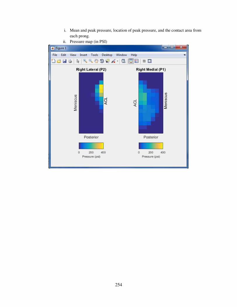
254

i. Mean and peak pressure, location of peak pressure, and the contact area from

each prong.

ii. Pressure map (in PSI)