Embed Size (px)
Citation preview
ABSTRACT
Title of Dissertation : PERFORMANCE ANALYSIS AND
HIERARCHICAL TIMING FOR DSP SYSTEM
SYNTHESIS
Nitin Chandrachoodan, Doctor of Philosophy, 2002
Dissertation directed by: Professor Shuvra S. Bhattacharyya (Chair/Advisor)
Professor K. J. Ray Liu (Co-advisor)
Department of Electrical and Computer Engineering
Improvements in computing resources have raised the possibility of spending
significantly larger amounts of time on optimization of architectures and schedules
for embedded system design than before. Existing design automation techniques
are either deterministic (and hence fail to make use of increased time) or use
general randomization techniques that may not be efficient at utilizing the time.
In this thesis, new techniques are proposed to increase the efficiency with which
design optimizations can be studied, thus enabling larger portions of design space
to be explored.
An adaptive approach to the problem of negative cycle detection in dynamic
graphs is proposed. This technique is used to determine whether a given set of
timing constraints is feasible. The dynamic nature of the graph often occurs in
problems such as scheduling and performance analysis, and using an adaptive

approach enables testing of more instances, thus increasing the potential design
space coverage.
There are currently no hierarchical techniques to represent timing information
in sequential systems. A model based on the concept of timing pairs is introduced
and studied, that can compactly represent circuits for the purpose of analyzing
their performance within the context of a larger system. An important extension
of this model also allows timing representation for multirate systems that allows
them to be treated similar to single rate systems for the purpose of performance
analysis.
The problem of architecture synthesis requires the generation of both a suitable
architecture and appropriate mapping and scheduling information of vertices.
Some approaches based on deterministic search as well as evolutionary algorithms
are studied for this problem. A new representation of schedules based on combining
partial schedules is proposed for evolving building blocks in the system.
PERFORMANCE ANALYSIS AND HIERARCHICAL TIMING FOR
DSP SYSTEM SYNTHESIS
by
Nitin Chandrachoodan
Dissertation submitted to the Faculty of the Graduate School of theUniversity of Maryland, College Park in partial fulfillment
of the requirements for the degree ofDoctor of Philosophy
2002
Advisory Committee:
Professor Shuvra S. Bhattacharyya (Chair/Advisor)Professor K. J. Ray Liu (Co-advisor),Professor Rajeev BaruaProfessor Gang QuProfessor Carlos Berenstein, Dean’s Representative

c© Copyright by
Nitin Chandrachoodan
2002

DEDICATION
To my Parents
ii

ACKNOWLEDGEMENTS
I would like to thank my advisors, Dr. Shuvra Bhattacharyya and Dr. Ray Liu, for
all the support and guidance they have provided me over the years. They granted
me tremendous freedom in choosing the final direction of my work, and this has
helped me form a much better balanced view of the work and why it is important.
I would also like to thank the various faculty from whose courses I benefited as
a student here, and the members of my dissertation committee: Dr. Barua, Dr.
Berenstein and Dr. Qu, for their helpful comments that have improved the quality
of the final work.
My research and stay in Maryland would not have been possible without
the funding provided through the various funding agencies over the years. In
particular, I would like to express gratitude for the funding through the following
sources: NSF Career Award MIP9734275, NSF NYI Award MIP9457397 and the
Advanced Sensors Collaborative Technology Alliance.
Over the past six years, I have had an excellent set of lab-mates to interact
with. I collaborated on design projects with Arun, Ozkan, Neal, Charles and John,
and these experiences taught me a lot about systematic digital design as well as
teamwork. I would like to thank Vida, Bishnupriya, Mukul, Ming-yung, Mainak,
Ankush, Sumit, Shahrooz and Fuat for a number of interesting discussions related
to CAD, and Masoud, Xiaowen, Jie Chen, Jie Song, Alejandra, Zoltan and Yan
from the signal processing group.
iii

I also had the good fortune to have a number of great roommates and friends
over this period: Prakash, Ganapathy, Sridhar, Arvind, Anand, Nagarajan,
Lakshmi, Vinod, Ameet, Kashyap, and of course, Jayant, from start to finish.
Friends from IITM: Ashok, Nagendra, Shami, Raghu, Srinath, Neelesh and
Srikrishna in particular. I owe you all a lot for companionship and moulding
my personality into whatever I am now.
I would not have been here without years of love and affection from a large
extended family consisting of a number of uncles, aunts, and cousins, to all of
whom I would like to convey my loving gratitude. To my sister, who has been
more of an inspiration as a stabilizing force than she probably realizes. To my
Mother, for everything that I cannot even begin to put into words. And lastly, to
my Father: though you are not with us now, I know you would have been very
proud. That alone makes this all worthwhile.
iv
TABLE OF CONTENTS
List of Tables 8
List of Figures 9
Chapter 1 Introduction 1
1.1 Embedded Systems . . . . . . . . . . . . . . . . . . . . . . . . . . . . . . . 1
1.2 Electronic Design Automation (EDA) . . . . . . . . . . . . . . . . . . . 3
1.2.1 High Level Synthesis . . . . . . . . . . . . . . . . . . . . . . . . . . 4
1.3 Contributions of this thesis . . . . . . . . . . . . . . . . . . . . . . . . . . 5
1.3.1 Adaptive performance estimation . . . . . . . . . . . . . . . . . . 7
1.3.2 Hierarchical Timing representation . . . . . . . . . . . . . . . . . 8
1.3.3 Architecture selection and evolution . . . . . . . . . . . . . . . . 9
1.4 Outline of thesis . . . . . . . . . . . . . . . . . . . . . . . . . . . . . . . . . 10
Chapter 2 High Level Synthesis 12
2.1 HLS design flow . . . . . . . . . . . . . . . . . . . . . . . . . . . . . . . . . 12
2.1.1 Representation . . . . . . . . . . . . . . . . . . . . . . . . . . . . . 14
2.1.2 Compilation . . . . . . . . . . . . . . . . . . . . . . . . . . . . . . . 18
2.1.3 Architecture selection and scheduling . . . . . . . . . . . . . . . 20
2.1.4 Optimization criteria and system costs . . . . . . . . . . . . . . 23
2.2 Design spaces . . . . . . . . . . . . . . . . . . . . . . . . . . . . . . . . . . . 25
v
2.2.1 Multi-objective optimization . . . . . . . . . . . . . . . . . . . . . 27
2.3 Complexity of the synthesis problem . . . . . . . . . . . . . . . . . . . . 30
2.3.1 Exact solution techniques . . . . . . . . . . . . . . . . . . . . . . . 31
2.3.2 Approximation algorithms . . . . . . . . . . . . . . . . . . . . . . 33
2.3.3 Heuristics . . . . . . . . . . . . . . . . . . . . . . . . . . . . . . . . . 33
2.3.4 Randomized approaches . . . . . . . . . . . . . . . . . . . . . . . . 35
2.3.5 Evolutionary algorithms . . . . . . . . . . . . . . . . . . . . . . . 37
2.3.6 Efficient use of compilation time computing power . . . . . . 38
Chapter 3 Performance analysis in dynamic graphs 40
3.1 Introduction . . . . . . . . . . . . . . . . . . . . . . . . . . . . . . . . . . . . 40
3.2 Performance analysis and negative cycle detection . . . . . . . . . . . 40
3.3 Previous work . . . . . . . . . . . . . . . . . . . . . . . . . . . . . . . . . . . 46
3.4 The Adaptive Bellman-Ford Algorithm . . . . . . . . . . . . . . . . . . . 52
3.4.1 Correctness of the method . . . . . . . . . . . . . . . . . . . . . . 54
3.5 Comparison against other incremental algorithms . . . . . . . . . . . . 59
3.6 Application: Maximum Cycle Mean computation . . . . . . . . . . . . 67
3.6.1 Experimental setup . . . . . . . . . . . . . . . . . . . . . . . . . . 68
3.6.2 Experimental results . . . . . . . . . . . . . . . . . . . . . . . . . . 71
3.7 Conclusions . . . . . . . . . . . . . . . . . . . . . . . . . . . . . . . . . . . . 78
Chapter 4 Hierarchical timing representation 80
4.1 Introduction . . . . . . . . . . . . . . . . . . . . . . . . . . . . . . . . . . . . 80
4.2 Need for hierarchical representations . . . . . . . . . . . . . . . . . . . . 81
4.3 Requirements of a Timing Model for Hierarchical Systems . . . . . . 85
4.3.1 SISO system . . . . . . . . . . . . . . . . . . . . . . . . . . . . . . . 85
4.3.2 Variable phase clock triggering . . . . . . . . . . . . . . . . . . . 87
vi
4.3.3 SDF Blocks . . . . . . . . . . . . . . . . . . . . . . . . . . . . . . . 87
4.3.4 Meaning of Timing Equivalence . . . . . . . . . . . . . . . . . . . 88
4.4 The Hierarchical Timing Pair Model . . . . . . . . . . . . . . . . . . . . 89
4.5 Data Structure and Algorithms . . . . . . . . . . . . . . . . . . . . . . . . 93
4.6 Multirate Systems . . . . . . . . . . . . . . . . . . . . . . . . . . . . . . . . 97
4.6.1 HTP model for multirate systems . . . . . . . . . . . . . . . . . 103
4.7 Relation of the HTP Multirate Model to other Models . . . . . . . . . 106
4.7.1 Synchronous Reactive Systems . . . . . . . . . . . . . . . . . . . 107
4.7.2 Cyclostatic Dataflow . . . . . . . . . . . . . . . . . . . . . . . . . . 107
4.7.3 RT-level hardware timing model . . . . . . . . . . . . . . . . . . 109
4.7.4 Discrete Time domain in Ptolemy II . . . . . . . . . . . . . . . . 109
4.8 Examples and Results . . . . . . . . . . . . . . . . . . . . . . . . . . . . . . 110
4.8.1 Multirate systems . . . . . . . . . . . . . . . . . . . . . . . . . . . 110
4.8.2 Single-rate systems . . . . . . . . . . . . . . . . . . . . . . . . . . . 111
4.9 Conclusions . . . . . . . . . . . . . . . . . . . . . . . . . . . . . . . . . . . . 115
Chapter 5 Architecture synthesis search techniques 116
5.1 Deterministic local search . . . . . . . . . . . . . . . . . . . . . . . . . . . 116
5.1.1 Fixed architecture systems . . . . . . . . . . . . . . . . . . . . . . 120
5.1.2 Experimental results . . . . . . . . . . . . . . . . . . . . . . . . . . 121
5.2 Genetic algorithms (GA) . . . . . . . . . . . . . . . . . . . . . . . . . . . . 126
5.2.1 GA for architecture synthesis . . . . . . . . . . . . . . . . . . . . 128
5.2.2 Range-chart guided genetic algorithm . . . . . . . . . . . . . . . 133
5.3 Operating principle of Genetic algorithms . . . . . . . . . . . . . . . . . 136
5.3.1 Schemata . . . . . . . . . . . . . . . . . . . . . . . . . . . . . . . . . 136
5.3.2 Fitness proportionate selection . . . . . . . . . . . . . . . . . . . 137
vii
5.3.3 Implicit parallelism . . . . . . . . . . . . . . . . . . . . . . . . . . . 139
5.3.4 Difficulties in using GAs for scheduling problems . . . . . . . 140
5.4 Partial Schedules: Building blocks for architecture synthesis . . . . . 144
5.4.1 Features of partial schedules . . . . . . . . . . . . . . . . . . . . . 145
5.4.2 Drawbacks of partial schedules . . . . . . . . . . . . . . . . . . . 147
5.5 Pareto front construction . . . . . . . . . . . . . . . . . . . . . . . . . . . . 149
5.6 Conclusions . . . . . . . . . . . . . . . . . . . . . . . . . . . . . . . . . . . . 150
Chapter 6 Conclusions and Future Work 153
6.1 Performance estimation . . . . . . . . . . . . . . . . . . . . . . . . . . . . . 153
6.1.1 Future directions . . . . . . . . . . . . . . . . . . . . . . . . . . . . 154
6.2 Hierarchical timing representation . . . . . . . . . . . . . . . . . . . . . . 155
6.2.1 Future directions . . . . . . . . . . . . . . . . . . . . . . . . . . . . 156
6.3 Architecture synthesis and scheduling . . . . . . . . . . . . . . . . . . . 158
6.3.1 Future directions . . . . . . . . . . . . . . . . . . . . . . . . . . . . 159
Bibliography 160
viii
LIST OF TABLES
3.1 Relative speed of adaptive vs. incremental approach for graph of
1000 nodes, 2000 edges. . . . . . . . . . . . . . . . . . . . . . . . . . . . . . 65
3.2 Run-time for MCM computation for largest ISCAS 89/93
benchmarks. . . . . . . . . . . . . . . . . . . . . . . . . . . . . . . . . . . . . 76
4.1 Tests for dominance of a path. . . . . . . . . . . . . . . . . . . . . . . . . 94
4.2 Timing pairs for multirate systems. . . . . . . . . . . . . . . . . . . . . . 112
4.3 Number of dominant timing pairs computed for ISCAS benchmark circuits. 112
4.4 HTP parameters for 10 largest ISCAS benchmark circuits. . . . . . . . . 113
5.1 Synthesis example results. . . . . . . . . . . . . . . . . . . . . . . . . . . . 122
5.2 Resource library for architecture synthesis. . . . . . . . . . . . . . . . . 132
5.3 GA-based evolution of schedules for Elliptic filter graph. . . . . . . . 132
5.4 Comparison of Range-chart guided GA vs. ABF based GA. . . . . . 135
ix
LIST OF FIGURES
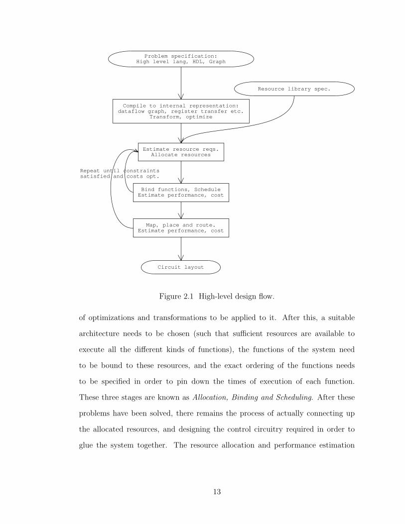
2.1 High-level design flow. . . . . . . . . . . . . . . . . . . . . . . . . . . . . . . . 13
2.2 Example of a Synchronous dataflow (SDF) graph. . . . . . . . . . . . . . 15
2.3 A deadlocked SDF graph. . . . . . . . . . . . . . . . . . . . . . . . . . . . . . 16
2.4 Cyclostatic dataflow graph. . . . . . . . . . . . . . . . . . . . . . . . . . . . . 17
2.5 Pareto-optimal set: All valid solution points are shown. . . . . . . . . . 29
3.1 Constraint graph. . . . . . . . . . . . . . . . . . . . . . . . . . . . . . . . . . . 58
3.2 Comparison of algorithms as batch size varies. . . . . . . . . . . . . . . . 64
3.3 Constant number of iterations at different batch sizes. . . . . . . . . . . 64
3.4 Asymptotic behavior of the algorithms. . . . . . . . . . . . . . . . . . . . . 66
3.5 Comparison of algorithms for 10,000 vertices, 20,000 edges: the
number of feedback edges (with delays) is varied as a proportion of
the total number of edges. . . . . . . . . . . . . . . . . . . . . . . . . . . . . 72
3.6 Performance of the algorithms as graph size varies : all edges have
delays (feedback edges) and number of edges = twice number of vertices. 73
3.7 Performance of the algorithms as graph size varies: proportion of
edges with delays = 0.1 and number of edges = twice number of
vertices (Y-axis limited to show detail). . . . . . . . . . . . . . . . . . . . . 74
3.8 Performance of the algorithms as graph edge density varies: all edges
have delays (feedback edges) and number of edges = 20,000. . . . . . . 75
x
3.9 Performance of the algorithms as graph size varies: proportion of
edges with delays = 0.1 and number of edges = 20,000. . . . . . . . . . 75
4.1 (a) Full adder circuit. (b) Hierarchical block view. . . . . . . . . . . . . . 82
4.2 Detailed timing of adder circuit. . . . . . . . . . . . . . . . . . . . . . . . . 86
4.3 Ripple effects with clock skew (multiple phase clocks). . . . . . . . . . . 88
4.4 Timing of complex blocks. . . . . . . . . . . . . . . . . . . . . . . . . . . . . 89
4.5 Second order filter section. . . . . . . . . . . . . . . . . . . . . . . . . . . . . 92
4.6 3 : 5 sample rate changer. . . . . . . . . . . . . . . . . . . . . . . . . . . . . . 99
4.7 Deadlock in multirate SDF system: if n < 10 the graph deadlocks. . . 102
4.8 Multirate FIR filter structure. . . . . . . . . . . . . . . . . . . . . . . . . . . 111
4.9 Binary tree structured QMF bank. . . . . . . . . . . . . . . . . . . . . . . . 111
5.1 Example of Chromosome structure for architecture synthesis GA. . . . 129
5.2 DFG where sequence 12435 is valid, but 13425 is not. . . . . . . . . . . 142
5.3 Example of a partial schedule. . . . . . . . . . . . . . . . . . . . . . . . . . . 144
5.4 A-T Pareto front for elliptic filter scheduling. . . . . . . . . . . . . . . . . 149
xi
Chapter 1
Introduction
We are living in an age where electronics is making the transition from novel to
commonplace. Less than one generation ago, household electronics were limited to
television sets and a few other such items that were valued as much for their novelty
as for their utility. Nowadays most people, at least in industrialized nations, use
electronic equipment so frequently as part of their everyday lives that they often do
not even notice them. The main factor driving this “ubiquitization” of electronics
is the development of systems where the processing elements are embedded within
a tool, and assist in the performance of the tool’s functions.
1.1 Embedded Systems
Embedded systems are found in a large number of applications. For example,
today even low-end cars contain several dozen processing elements, that take care
of various elements of control, such as fuel-injection, anti-lock braking systems,
temperature and seat-comfort, and navigational assistance, among other things.
In the household, television sets and recorders have programmable settings that
allow them to be turned on or off at set times or for specific programs, and also
allow control over what programs can be seen. Similar functionality exists for
1
appliances such as microwave ovens and toasters to control their operation. In all
these applications the embedded computing system plays the role of a controlling
device. It provides the ability to choose between several modes of operation that
are available for the device in question.
A different kind of functionality is desired in embedded systems that process
data streams. Typical examples of such systems are cellular phones, modems and
multimedia terminals. These devices usually have two aspects: one is to provide
choice between different kinds of functionality in a manner similar to the devices
above. The other aspect is to process a data stream. For example, in a cell-
phone, it is necessary to sample the data decoded from the radio receiver, and
convert it into appropriate voice or data samples, while minimizing the errors in
the reception. For transmission of data, similar operations need to be performed in
order to provide error protection or encryption for security. Multimedia terminals
and video-conferencing equipment also deal with images being transmitted, and
in these cases there may be other operations, such as scaling the image to an
appropriate size for display, apart from the main tasks of encoding and decoding
the images for efficient transmission and reception.
Designing and implementing such electronic systems involves several stages.
First an algorithm needs to be chosen that operates on the inputs available to
the system, and is able to produce appropriate outputs. For example, certain
control functionality, like user interfaces, could be implemented as a finite state
machine. For signal processing applications, the algorithms may require extensive
tuning based on observed channel and signal characteristics, and the encoding and
decoding system may need to be chosen appropriately.
Once the algorithm has been decided upon, the next stage is to implement
an electronic circuit that is capable of executing the required task. This has
2
typically been done by hand. Experienced designers choose either an electronic
(hardware) implementation, or suitable computing and interface elements together
with software, such that the required functionality can be obtained from the
system. The quality of the design is largely determined by the experience of
the designer.
1.2 Electronic Design Automation (EDA)
The current trend towards increased availability of computing power for a given
size and cost means that it is possible to implement ever more complex tasks in a
small area. As a result of this, algorithm and system designers have the freedom
to pack more functionality into a given unit. As the size of the circuit grows, it
becomes increasingly difficult for a human designer to keep track of all possible
implementation options and to make the best choice of system design.
Several tools currently exist that help the designer in the process of evaluating
an algorithm to implement and proceeding through all the stages of the design.
In particular, the last stages of actually optimizing and laying out a circuit once
it has been described at a sufficient level of detail has been well-studied, and
several excellent tools exist for this logic-minimization problem. Examples include
the Synopsys Design Compiler [105] and the Cadence design systems [19] layout
and synthesis tools. Many of the commercial tools in existence today are based
on earlier academic tools for synthesis and design, such as SIS [103] and Hyper-
LP [24] from the University of California, Berkeley, the Olympus [76] CAD system
from Stanford University and the Ocean [53] tools from Delft University. Most
of these tools work at the level of circuits and gate-level netlists, though some of
them, such as Synopsys Behavioral Compiler, incorporate techniques to operate
3

at higher levels of abstraction.
It is desirable to develop design methodologies that encompass the entire design
flow from system-level description down to actual hardware implementation in a
single design tool or environment. The advantage of such a system is that it
allows a single designer to get a better overall view of the system being designed,
and opens up the possibility of much better overall designs [25], based on cost
considerations as discussed in sec. 2.1.4. A very important additional goal is that
the overall “Time-to-Market” of the design can be greatly reduced, and this is
a crucial factor in determining the economic viability of any system. Another
factor, as mentioned in [25, 69], is the fact that more power-efficient designs can
be made by making appropriate decisions at a higher level of the design, than by
concentrating on circuit level improvements.
The ultimate goal is to have a single tool that can take abstract designs and go
through the entire process of system design automatically. In the near term, it is
equally or more important to consider techniques that aid the designer by exploring
large parts of the design space automatically, and presenting a set of useful designs
to human designers, who can then use their experience to choose a suitable
candidate. Automatic tools can also help by taking a candidate design generated
by human experience, and exploring all the variations that might improve this
design. Electronic Design Automation (EDA) tools are software tools and libraries
that attempt to make this kind of systematic design possible.
1.2.1 High Level Synthesis
The main goal of a human designer in a system design environment should be
to make decisions that affect the overall functionality of the system. The actual
task of obtaining the required performance, and tuning the parameters for efficient
4
operation, should be taken care of by automatic synthesis tools. This in turn means
that it is desirable to describe the system in as abstract a manner as possible, and
use automatic tools to fill in the details and obtain a specific working design. This
is the basic idea behind High Level Synthesis (HLS).
In HLS, the problem is described at a high level of abstraction. The process
is discussed in further detail in the next chapter (2), but typical methods include
the use of hardware description languages, or flow-graph related techniques. The
available choices of hardware are described in terms of implementation libraries
that consist of collections of resources capable of executing the different functions
required for operation of the system. The goal of an automated synthesis system is
to select suitable resources and map the desired functionality to this architecture,
and to generate any control circuitry that is required for correct operation.
The main problems here are related to the complexity of the various sub-
problems that need to be solved for the synthesis problem. Chapter 2 gives an
overview of the various issues involved, together with a look at existing approaches
for solving the problems. It also tries to motivate the need for randomized design
space exploration methods that are capable of searching through several different
combinations of designs in order to find the best implementation.
1.3 Contributions of this thesis
As will be seen in Chapter 2, it is often desirable to use efficient randomized search
techniques that can explore the design space of a high-level synthesis problem. In
this regard, there are also a number of issues related to problem representation and
analysis methods, that need to be addressed in order to improve the performance
of these techniques.
5

In this thesis, we identify some of these problems, and present better methods
for attacking them. The main areas we look at are:
• Analysis techniques: The primary goal of the design tool is to construct
a potential solution, and then analyze its performance to see if it
meets requirements. This requires efficient techniques for estimating the
performance of the system, as well as understanding of other factors that
can speed up this process. We present an adaptive approach to the problem
of constraint analysis in chapter 3, that aims to streamline the processes of
scheduling and estimating performance metrics.
• Timing cost representation: It should be possible to compactly depict large
designs, and also to hide the internal complexity of design elements so that
the system-level tool can work with a high-level view of the system. This
reduces the size of the problem that the tool works on, and therefore enables
faster analysis, and consequently, larger percentage of the design space can
be explored. Hierarchical timing representation is crucial to this effort.
In chapter 4, such a hierarchical approach is presented for sequential and
multirate systems.
• Evolutionary architecture improvement: Evolutionary algorithms are a very
useful technique for exploring large design spaces. However, choosing a
suitable encoding and mapping scheme for a genetic algorithm are difficult,
especially for the problems in scheduling that are based on sequencing in the
presence of constraints. We therefore consider a new encoding technique in
chapter 5 that is closely related to the underlying structure of the scheduling
problem.
6
1.3.1 Adaptive performance estimation
In this section, sec. 1.3.1, we briefly outline the problem of performance estimation,
the advantages that can be obtained through an adaptive approach to this problem,
and the approach we have used to make this process more efficient. The technique
we develop, adaptive negative cycle detection, is studied in chapter 3, where
we compare the approach with other incremental approaches, and present an
application of this approach to fast computation of the maximum cycle mean
metric.
The most important constraint in an electronic system design is to ensure that
it runs “fast enough”. The minimum speed required of the circuit is often set by
external constraints such as the sampling rate of the input data, or the required
frame rate for video image processing. For certain kinds of off-line algorithms, such
as some types of MPEG video encoding, the algorithm may not need to function
within a deadline, but even here it is desirable to execute as fast as possible.
As a result of this, timing constraint analysis is a very important part of
EDA, and is one of the most used functions in the process of evaluating a circuit
implementation. In general, the constraints of a circuit can be described as a set of
linear difference constraints, and a solution to this set provides a schedule (exact
start times) for all the operations. It is possible to devise synthesis algorithms that
operate by the process of systematically generating several different sequences of
the operations, and testing the result for constraint satisfaction.
In such situations, we need to repeatedly verify constraint satisfaction on a
set of related graphs (where the constraint system is represented as an equivalent
graph). These graphs differ from each other in only a small part of the overall
set of constraints. It is desirable to use analysis techniques that are able to make
7

use of previously computed results for constraint satisfaction in order to make the
current results more easy and fast to compute.
The work we present uses the concept of Adaptive negative cycle detection on
such dynamic graphs to speed up the process of evaluating the performance of
the system. It is shown that when we consider changes to the system graph that
consist of multiple simultaneous changes to the graph structure (as is the case in
several problems in design automation and performance analysis), the adaptive
approach derived from the Bellman-Ford algorithm for shortest path computation
is more efficient than existing incremental approaches.
The maximum cycle mean (MCM) of a graph is a bound on the minimum
iteration period that can be used for clocking the underlying circuit. An important
application of adaptive negative cycle detection is that it can be used to derive a
very efficient implementation of Lawler’s algorithm for computing the MCM [64,
35].
1.3.2 Hierarchical Timing representation
The analysis of the system performance referred to above works on the timing
information associated with the elements of the design. In general, timing
information is used for the purpose of generating a set of constraints related to
the graph, and analyzing these constraints allows us to decide on the feasibility or
usefulness of a design.
Normal combinational circuits use a simple approach based on computing
longest paths through the circuit to compactly represent the overall timing of
complex blocks. This approach fails for sequential circuits (that have register/delay
elements), and for multirate circuits (like certain kinds of signal processing
applications). This compact representation is, however, very desirable, and even
8

necessary, in order to extend the analysis techniques to large designs.
In chapter 4, we present an approach based on the concept of constraint
time, which uses a list of pairs of numbers to represent the information that is
required to compute the timing information of a sequential circuit for the purpose
of performance analysis. This has the potential to make it possible to handle much
larger designs.
An additional important advantage of the hierarchical timing pair model is
that a similar model can be defined for multirate systems. This enables us to treat
multirate systems in a manner similar to normal single rate systems, and certain
results on performance bounds of single rate systems can now be extended to
multirate systems. This should make it easier to analyze and design such systems
in future.
1.3.3 Architecture selection and evolution
The final goal of an HLS system is to generate both an architecture (allocation
and binding of resources) and schedule (ordering of functions on resources), that
is capable of executing all the function required for a particular application within
the constraints imposed on it. In addition, it is desirable to then minimize any
other costs that have not been explicitly constrained. A typical example is to
design an architecture and schedule that meets timing and area constraints, and
minimizes the power consumption subject to these constraints.
Due to the complexity of the problems in HLS as discussed in the next chapter,
it is often necessary to look for non-deterministic approaches to design space
exploration. The most popular methods for this are evolutionary approaches such
as genetic algorithms. These algorithms are somewhat difficult to use effectively
for sequencing problems such as scheduling. Repairing or penalizing invalid
9
chromosomes often leads to situations involving either a bias in the search space,
or a very low efficiency due to too many candidates being discarded.
In Chapter 5, we consider several approaches to architecture selection based
on randomized search techniques. Some of these are based on search techniques
that make use of the adaptive negative cycle detection technique, while others are
derived from previously known techniques for scheduling iterative graphs.
In addition to this, we look at a new representation of an architecture in terms
of partial schedules. These enable us to represent part of a solution in a way that
makes it possible to mix and match different partial schedules to obtain a complete
schedule. We study these schedules, and show how they can provide a useful basis
to tackle the problem of architecture synthesis.
1.4 Outline of thesis
The outline of this thesis is as follows: Chapter 2 presents an overview of the high-
level synthesis problem and identifies difficulties associated with current techniques
for design space exploration. Chapter 3 looks at the problem of timing constraint
analysis in the context of dynamic graphs, and presents techniques and results
that show the improvements we can obtain with these techniques. Chapter 4
considers the problem of hierarchical timing representation for sequential systems
and presents the timing pair model that attempts to provide a solution to this
problem. It also shows how to extend the hierarchical timing pair concept to
multirate systems, and shows how the performance analysis techniques on single
rate systems can now be extended to multirate systems. Chapter 5 looks at several
different evolutionary techniques for synthesis of architectures with different cost
constraints, and also introduces a new schedule encoding technique that aims
10

to eliminate some of the problems associated with encoding schedules for GAs.
Finally, chapter 6 summarizes the results and looks at possible directions for future
work.
11

Chapter 2
High Level Synthesis
High level synthesis (HLS) refers to the process by which a system represented
at a high level of abstraction is converted into a circuit level implementation by
automatic tools.
The overall design process consists of several stages, as described in sec. 2.3.
In this work, we are most interested in a design flow that works at the higher
levels of abstraction, without worrying about the final implementation and low-
level optimization details. This is reasonable because the low-level design problem
has been extensively studied for several years, and has many approaches to solve it.
The high-level design process is currently less well studied, but has the potential
for promoting greater overall design efficiency [25, 69].
2.1 HLS design flow
The complete process of automated system design can be broken into a number
of stages, arranged in a design flow as shown in figure 2.1.
The HLS process begins by describing the required functionality using
an appropriate description language at a suitable level of abstraction. This
description is then compiled into an internal representation that allows a number
12
Problem specification:High level lang, HDL, Graph
Compile to internal representation:dataflow graph, register transfer etc.
Transform, optimize
Resource library spec.
Estimate resource reqs.Allocate resources
Bind functions, ScheduleEstimate performance, cost
Map, place and route.Estimate performance, cost
Circuit layout
Repeat until constraintssatisfied and costs opt.
Figure 2.1 High-level design flow.
of optimizations and transformations to be applied to it. After this, a suitable
architecture needs to be chosen (such that sufficient resources are available to
execute all the different kinds of functions), the functions of the system need
to be bound to these resources, and the exact ordering of the functions needs
to be specified in order to pin down the times of execution of each function.
These three stages are known as Allocation, Binding and Scheduling. After these
problems have been solved, there remains the process of actually connecting up
the allocated resources, and designing the control circuitry required in order to
glue the system together. The resource allocation and performance estimation
13

usually need to be iterated several times to meet the constraints. This is then
translated into silicon circuitry that needs to be laid out and routed for fabrication
on appropriate design processes. This introduces additional variations in the cost
and performance, because of wiring costs and routing overhead. Both these stages
provide information on costs that can be used by the previous resource allocation
stage to improve the allocation iteratively.
In the next few sections, we look at available methods for tackling each of these
problems individually.
2.1.1 Representation
The first problem to be tackled for HLS is representation. It is required to provide
a model of the algorithm in a manner that lends itself to analysis as well as to
transformations that reveal better properties that can be exploited for improving
performance. In this section, we consider existing approaches for representing
algorithms and circuits at a high level of abstraction, and try to motivate our
choice of a dataflow based model (in particular variants of the SDF model) for
this purpose.
Some of the methods used for representing algorithms include control-dataflow
graphs [37] and languages such as SIGNAL [54] and ESTEREL [9]. Graphical
techniques such as Statecharts [55], and dataflow graphs as used in the Ptolemy [17]
environment are very popular due to the ease of use and their ability to capture
complex ideas. These representations can be compiled into internal formats that
can then be used for analysis of properties of the underlying system. Petri nets [79]
are a graph based representation that allows mathematical analysis of many of the
properties of such systems. In addition, ideas such as system property intervals
(SPI) [30] are used to extend the capabilities of dataflow systems to represent
14
A
B C
3
5
23
10
4
10D
Figure 2.2 Example of a Synchronous dataflow (SDF) graph.
information about a system.
Systems are often described using high-level hardware description languages
such as VHDL [59, 3], Verilog [110] or System C [106]. These languages have
the advantage in being similar, from a programming point of view, to well known
software programming languages. They are augmented with certain constructs
that allow easy representation of concurrency. By using either a structural or a
behavioral mode of description, it is possible to either directly encode gate level
designs, or describe the design at a high level of abstraction in terms of familiar
mathematical and logical constructs.
One of the most important representation schemes for signal processing systems
is based on the idea of dataflow graphs [66, 37]. Dataflow graphs are particularly
well suited to signal processing applications because signal processing systems tend
to consist of a standard set of operations being executed on a semi-infinite input
stream.
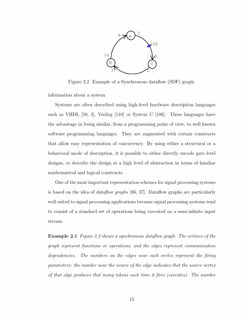
Example 2.1 Figure 2.2 shows a synchronous dataflow graph. The vertices of the
graph represent functions or operations, and the edges represent communication
dependencies. The numbers on the edges near each vertex represent the firing
parameters: the number near the source of the edge indicates that the source vertex
of that edge produces that many tokens each time it fires (executes). The number
15
A
B C
3
5
23
10
4
9D
A
B C
3
5
23
10
4
10D
(a) Functional SDF Graph (b) Deadlocks after 1 firing
1D
Figure 2.3 A deadlocked SDF graph.
near the sink vertex indicates the corresponding token consumption rate. An edge
can have a certain number of initial tokens (represented by a diamond and the
corresponding number), which indicates inter-iteration dependency, and can permit
the sink vertex to fire sooner since it provides initial tokens.
In the example shown, the firing sequence CCBAACBAAA will bring the system
back to the state shown in the figure. This means, first C executes twice, consuming
5 tokens each time, and producing a total of 4 tokens on edge CB, then B executes
once, then A twice, and so on.
The synchronous dataflow (SDF) model [66] is a well studied method for
representing DSP systems. The major advantage of this approach is that it also
provides a convenient method for representing and analyzing multirate [112, 69]
systems that are found in DSP. Unfortunately, although this method provides
some useful techniques to study software implementations of these graphs, it makes
certain assumptions about the execution of individual functions in the graph that
can lead to deadlocked graphs in certain cases. As a result, alternative approaches
have been proposed that try to avoid the deadlock problem, such as cyclostatic
dataflow [12], and alternative interpretations of the firing rules on these graphs as
periodic signals [43].
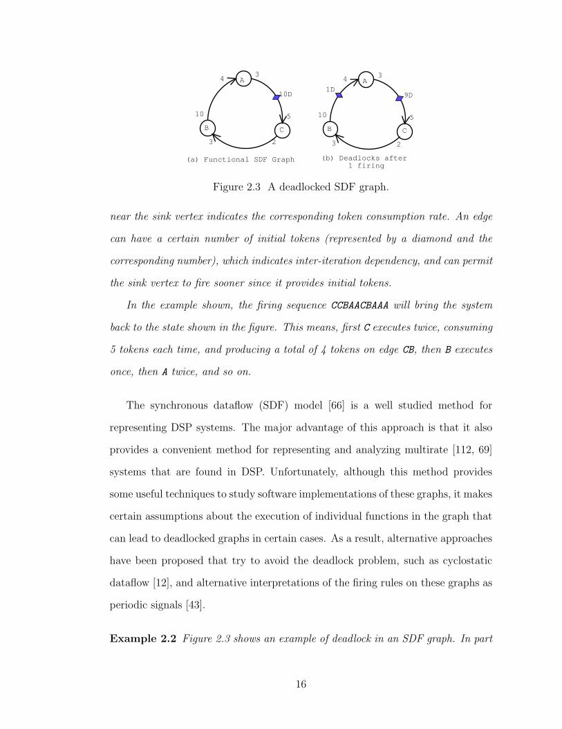
Example 2.2 Figure 2.3 shows an example of deadlock in an SDF graph. In part
16

[1,0]
[0,1]
[1,1]
Figure 2.4 Cyclostatic dataflow graph.
(a), as we saw in Example 2.1, we have the valid firing sequence CCBAACBAAA.
There are also other sequences that are possible, and that will bring the system
back to its original state after a certain number of firings.
In part (b) of the figure, on the other hand, the initial tokens have been
redistributed so that the token count on edge AC is only 9 instead of 10. This means
that vertex C can fire only once to start with, producing only 2 output tokens. This
means that vertex B will never be activated.
Even if the token count on edge BA is increased to 3, the system is still
deadlocked, in spite of having a greater total number of initial tokens than in
part (a). It is important to note that this deadlock is not necessarily an inherent
property of the system under consideration: rather, it is brought about due to the
firing rules that are used to determine the execution sequence.
Example 2.3 Figure 2.4 shows an example of a cyclostatic representation. The
figure on the left is a commutator switch, whose function is to transmit its 2
input streams alternately onto the output stream. It is not possible to completely
represent this behavior in SDF, because the alternate input selection is a time/data
dependent operation that cannot be modeled in SDF.
The cyclostatic representation models this using phases. In the first phase,
one of the edges (with 1 as the first phase), sends its data to the output, while
the other edge (with 0 as its first phase) consumes no tokens. In the second
17
phase, the consumption parameters are switched around. In this way, the CSDF
representation efficiently models the time-dependent nature of the operation.
At the same time, the changes made by the CSDF model to SDF are minimal.
So it is still able to use many of the properties of the SDF model. This makes it
a good choice for modeling multirate systems or periodically time variant systems
that have time-dependent, but cyclic execution patterns.
In this thesis, we consider the SDF model as the basis for representation and
analysis, because it has a rich history and has been well studied. However, for the
timing pair representation for multirate systems (sec. 4.6.1), we will change the
interpretation of the firing rules, and develop a model that is more natural and
efficient for hardware implementation of dataflow graphs.
Once the graph representing the computation and communication
dependencies has been described using one of the above methods, it is also
required to annotate it with information about the execution times and other
costs of the various elements involved. These costs depend on the actual choice
of what hardware element we schedule each operation on. Also, the actual cost
of the overall system may not be just a simple sum of the costs of the individual
elements.
2.1.2 Compilation
The first step in processing is to convert the input format into an internal format
amenable to analysis and transformation. The SDF and related dataflow formats
are commonly used as internal formats as they provide a good mathematical model
for analysis. In this section, some pointers to resources discussing these aspects in
further detail are given.
18
The compilation and mapping proceeds by transforming the dataflow graph to
reveal more parallelism or other useful properties, and mapping the graph onto a
set of resources from a library, taking into account costs as described in sec. 2.1.4.
A number of transformations can be applied to graphs to expose parallelism,
many of which are discussed in [85]. These include unfolding, look-ahead
and operator strength reduction along with other techniques often used in
compiler design such as common subexpression extraction, dead-code elimination
etc. Retiming [67, 118, 100] is a useful transformation used for synchronous
circuitry. Other techniques such as the multirate transform [69] have more limited
applicability (mainly to filtering or transform applications). These transforms
convert the application graph into a format where the concurrency of different
sections is made more clear, and this allows synthesis tools to choose better
implementations.
For the purpose of compilation and transformation, it is required to have some
knowledge of the performance and cost of the functions and resources available.
It is possible to model these costs in different ways. For example, a realistic
power model requires taking into account the switching activity of the signals
in a system [26]. Another, simpler alternative, is to use additive models, where
each resource is assumed to occupy a certain area, incur a certain cost, and have
a certain amount of power consumption that only depends on what function is
executed on this resource at a given time [73, 99].
Most system-level synthesis approaches require the input to be represented in
some graph based format that allows such transformations. Compilers are used
to convert other formats, such as hardware description languages like Verilog or
VHDL into an internal graph based structure for synthesis. Graph-based formats
have the advantage that several tools such as Ptolemy [17] and commercial tools
19

like SPW [18] from Cadence systems and Cossap [104] from Synopsys support
graphical entry and simulation, and this manner of entry makes the generation of
a graph-based internal format more easy and natural.
For the rest of this thesis we will assume that our input problem is provided as
a dataflow graph (either SDF or appropriate variants depending on the context).
The resource libraries use the simple additive power and area models, although
in most cases it should be possible to extend them to more complex and accurate
models without loss of generality, as the techniques that we develop do not, in
general, depend on the details of the cost models.
2.1.3 Architecture selection and scheduling
Along with the algorithm specification (which we assume is represented as a
dataflow graph), we need a set of resources onto which the functions are to be
mapped. We first need to select an appropriate set of resources and then schedule
the operations on these resources so as to meet the various constraints on the
performance of the system. In certain cases, such as scheduling for a fixed type
of multiprocessor architecture, the allocation is already decided by the target
platform. In this case, the problem reduces to scheduling, but it may still be
necessary to consider costs such as inter-processor communication costs.
Ideally, the three problems of allocation, binding and scheduling should
be solved simultaneously, because decisions on allocation affect availability of
resources, thereby affecting the execution times of functions, which in turn
constrains the minimum hardware requirements for synthesis of the system.
However, it is known that even the scheduling problem by itself is computationally
hard [47], and due to the interaction between the stages, it is not possible to
solve the allocation and binding stages optimally without taking into account the
20
scheduling information. Therefore, in order to keep the complexity of the problem
under control, they are usually addressed one after the other.
Several approaches exist for the scheduling problem, with many of the most
useful ones being based on the idea of priority lists [37, 86]. These use a priority
list to define an ordering of the nodes in the graph, and use an algorithm that
selects each function in order of priority for scheduling on an appropriate resource.
In most cases, the resource type binding needs to be known in order to compute
the priorities, so the allocation and binding steps need to be performed in advance.
The typical approach in such situations [86] is to perform an allocation based on
some loose bounds that can be established on the system requirements, try to
schedule on this system, and then use information from this scheduling step to
improve the allocation.
Force-directed scheduling [86] uses the concept of a “force” between operations
as a measure of the amount of concurrency in the system. This has been found
to be very effective in minimizing resource consumption in a latency constrained
system, or alternatively can also be used to minimize latency on a set of fixed
resources.
Clustering techniques [115, 98] are another approach used in multiprocessor
and parallel processing systems. These are most relevant in situations where
a homogeneous processing element is used for all functions, and it is required
to control the communication costs between elements scheduled on different
processors. Clusters of tasks are grouped together, with the idea being that tasks
on the same processor do not incur a mutual communication cost, and by choosing
the clusters efficiently, it should be possible to obtain an efficient implementation
that has low communication cost.
Most of the techniques described previously, and indeed, most existing research
21
in this field, is focused on acyclic graphs, where the metric of timing performance
is the “latency” of the graph, or the critical path through the graph. There are
several reasons why such graphs are more popular:
• Many task graphs in parallel applications are single-run task graphs that do
not exhibit inter-iteration parallelism.
• Acyclic graphs are easier to handle than cyclic graphs, as the problems of
deadlock etc. do not arise. Computing the longest path is also a simpler
problem, and faster to execute, than computing the maximum cycle mean,
which is the equivalent metric of performance in a cyclic graph.
• It is possible to convert a cyclic graph into an acyclic graph by removing
the feedback edges (with delay elements on them). However, this can lead
to performance loss unless techniques like unfolding are used to expose
parallelism in the graph. Such transformations increase the size of the graph,
and can lead to significant increase in complexity.
Because of the fact that certain solutions may be missed in treating a cyclic
graph as an acyclic one, there have been several attempts at dealing with cyclic
graphs directly. SDF graphs have been successfully used for modeling DSP
applications and several useful results have been derived [66, 11, 118] for such
graphs. Optimum unfolding [84] is one technique that has been proposed for
generating optimal schedules for cyclic graphs by means of unfolding them by an
appropriate factor. As mentioned previously, this can potentially lead to large
increases in the size of the resulting graph. Schwartz and Barnwell proposed
the idea of cyclostatic schedules [102] as a new way of looking at schedules for
iterative graphs, and used a full search technique to explore the design space to
obtain suitable schedules.
22
Range-chart guided scheduling for iterative dataflow graphs [36] is one of the
few attempts at directly scheduling a cyclic dataflow graph without converting to
an acyclic graph or unfolding it. This uses the concept of range charts, similar
to the idea of “mobility” in other list scheduling techniques. The range charts
indicate stretches of time within which a given operation can be scheduled, and by
searching through this, it is possible to obtain good locations for scheduling each
operation. This method tries to minimize the resource consumption for a fixed time
constraint. This method explicitly tries to minimize the resource consumption for a
given target iteration period by searching through the possible scheduling instants
for the operations. As a result, it can only be used when the execution times
of the operations are relatively small integers, and is also not easy to extend to
optimization of other cost criteria such as power.
2.1.4 Optimization criteria and system costs
For an EDA tool to successfully generate a suitable design from a set of
specifications, it must be able to select design elements from appropriately
annotated resource libraries. These libraries require information about the
functionality of the elements, as well as about the cost incurred along various
dimensions of interest. The primary costs of concern in most electronic designs
are:
• Time: Since most applications (especially for signal processing) require data
to be processed within certain deadlines, the amount of time taken to execute
different tasks is important.
• Area: For a hardware realization of an algorithm, the primary cost is the
area consumed by the elements on an integrated circuit (VLSI) chip. For
23

software realizations, the code size, data size or buffer requirements could be
taken as an equivalent measure.
• Price: Although usually the price of the realization and the area would be
related, this may not be the case when it is desirable to use commercial off-
the-shelf (COTS) components. Such components can be used to bring down
the cost and prototyping time of the design, although they may result in a
design that is not the most compact.
• Power: Power consumption is rapidly becoming one of the most important
cost criteria [25, 69]. This is mainly driven by the demand for handheld and
portable devices. Such devices require low power consumption in order to
extend battery life, and to reduce the weight of the batteries required to keep
them operational for suitable periods of time.
Most early research on design methodologies focused on the problems of either
time minimization (obtain the fastest implementation given a set of resources), or
area minimization (smallest design that meets the timing constraints) [86, 37, 48].
This was most relevant when silicon area was extremely precious, and it was
required to squeeze as much performance out of a system as possible.
Nowadays, although silicon is still a precious resource, very high levels of circuit
integration [74, 49, 114] have made it possible to consider trading off chip area in
order to obtain lower power consumption [25, 69]. Alternately, it may be possible
to trade off area for speed, and even use multiple parallel implementations and
other algorithmic transformations to obtain high throughput [85].
It has been observed [25] that performing optimizations at a higher level of
abstraction can lead to much higher savings in the power consumption than could
be obtained by any amount of optimization at a logic or circuit level. The papers
24

by Liu et al. [69] and Parhi [85] consider techniques of transforming the circuit
description at the algorithm and architecture level (very close to the highest system
level) since optimizations at these levels have been shown to result in much greater
power and cost savings than the fine grained tuning that is possible at the circuit
or logic level.
It is clear that it would be desirable to have design tools that accept inputs
at very high levels of abstraction, and are able to take them all the way to silicon
implementations. However, so far there has been only limited success in attempts
to create such tools. Most existing EDA tools break up the design process into a
number of distinct stages in order to simplify them. This makes it more difficult
to apply system level optimizations that can lead to the best results.
2.2 Design spaces
Design space is a term used to aid in understanding the process of searching for
solutions to complex combinatorial problems such as architectural synthesis. The
main concept here is that we treat every variable entity in the design as a different
dimension, and this entity can take on one of a fixed (possibly infinite) values in
each solution instance.
Every candidate solution to the problem has a certain set of values assigned
to its variables. In this way, each candidate can then be uniquely identified by
specifying all the values of these variables. We can visualize this as the candidate
solution being a point in a multi-dimensional space whose axes are specified by
the variables.
Example 2.4 Consider the optimization problem where it is desired to find the
minimum value of a function f(x, y) where x and y are variables that can take
25
values in the range (−∞, +∞).
In this instance, the design space is defined by the whole surface spanned by
the ranges of the variables x and y. Any point such as (2.718, 3.1415) or (10, 10)
is a candidate solution to the minimization problem, and therefore a point in the
design space.
Example 2.5 Consider a dataflow graph with vertices v1, v2, . . . , vn, and a set of
resource types r1, r2, . . . , rR.
An allocation of resources for synthesizing this system would consist of certain
resource instances, which can be denoted as Ii,j where i is the resource type (i ∈{ri}), and j is the instance number. In this way, I1,2 would indicate the second
instance of a resource of type 1.
The binding of functions to resources can be represented by a mapping b(v)
where v refers to the index number of the vertex in question. This would take
values of the form Ii,j to indicate that vertex v is mapped onto the resource instance
Ii,j.
The scheduling of the vertices could further be indicated using a mapping such
as ts(v) to indicate the start time of each vertex. ts(v) would then take on a real
(or integer, depending on whether timing refers to true time or clock ticks) value
for each scheduled vertex.
The data points {Ii,j}, {b(v)} and {ts(v)} together completely specify an
architecture and schedule for a system.
Note that it is not necessary that the values refer to valid instances. For
example, as far as the design space is concerned, it is perfectly acceptable to
map vertex v onto instance I3,4 (4th instance of resource type 3), even though
in the allocation, only 2 instances of resource type 3 were allocated. This would
correspond to a point in the design space that would then be considered as having
26

infinite cost, as it is infeasible.
Design spaces help to visualize the process of searching for an optimal solution.
In a continuous optimization problem such as example 2.4, it is possible to use
analytical methods such as gradient descent, or even finding the points where the
derivative of the function to be optimized becomes 0. In a discrete (combinatorial)
optimization problem, this may not in general be possible. In general, the cost
function may be highly irregular over the design space. It is not possible to define
useful derivatives or use gradient descent techniques effectively in such cases.
Another problem with irregular search spaces is the existence of multiple local
minima. That is, there could be several points that appear to minimize the
function, because all points around them (obtained by changing one or more
dimensions by small amounts) have worse costs than the point considered. Since
several search techniques are based on the idea of improving a solution that meets
some of the constraints, these local minima can pose serious problems, since it
is not usually possible to migrate from one local minimum to another without
passing through some points of worse cost.
The irregular nature of these design spaces is one of the important reasons
for choosing probabilistic optimization algorithms: these have a certain non-zero
probability of moving out of local minima, which is not possible with deterministic
algorithms unless we explicitly decide to accept temporary worsening of solutions.
2.2.1 Multi-objective optimization
As we saw above, the design space is multidimensional, and could in general be
a space of very high dimensionality. However, what we are really interested in
optimizing is the cost of the solution. For a synthesis problem, possible costs
27
that we want to optimize are throughput (possibly related to latency), area, price
of parts, and total power consumption. These costs are usually related to each
other in very complex ways depending on the interaction of the functions and
resources in the schedule. Therefore, it is not possible to minimize, say, the power
consumption, without having to sacrifice either the throughput or the size (area)
of the solution.
In a multi-objective optimization problem, there may not be a unique
solution that optimizes all the costs [83]. Therefore the cost criterion has to be
appropriately re-defined to make meaningful judgments of the quality of a solution.
There are several ways of handling this, a few of which are mentioned below (more
details can be found in [41, 5]) :
• Weighted cost function: Instead of optimizing each of the costs separately,
the costs (such as area, time and power) are combined into a single cost
using some function (usually a linear weighted combination of the costs).
In this way, it is possible to control the importance given to one of the cost
dimensions by giving it a higher or lower weight, and the overall optimization
process can concentrate on a single cost function. A major drawback of this
approach is that there is often no meaningful way to add different metrics
together, as they refer to different aspects of cost such as time and power.
• Hierarchical optimization: The different costs are ranked in order of
importance, and the optimization is done sequentially. At each stage, we
can sacrifice some amount of optimality on previous criteria to get a better
optimum for the combined optimization.
• Goal oriented optimization: Some of the costs are converted into constraints
that need to be satisfied. This means that the overall system can eventually
28
Pareto optimal point
Candidate solutions
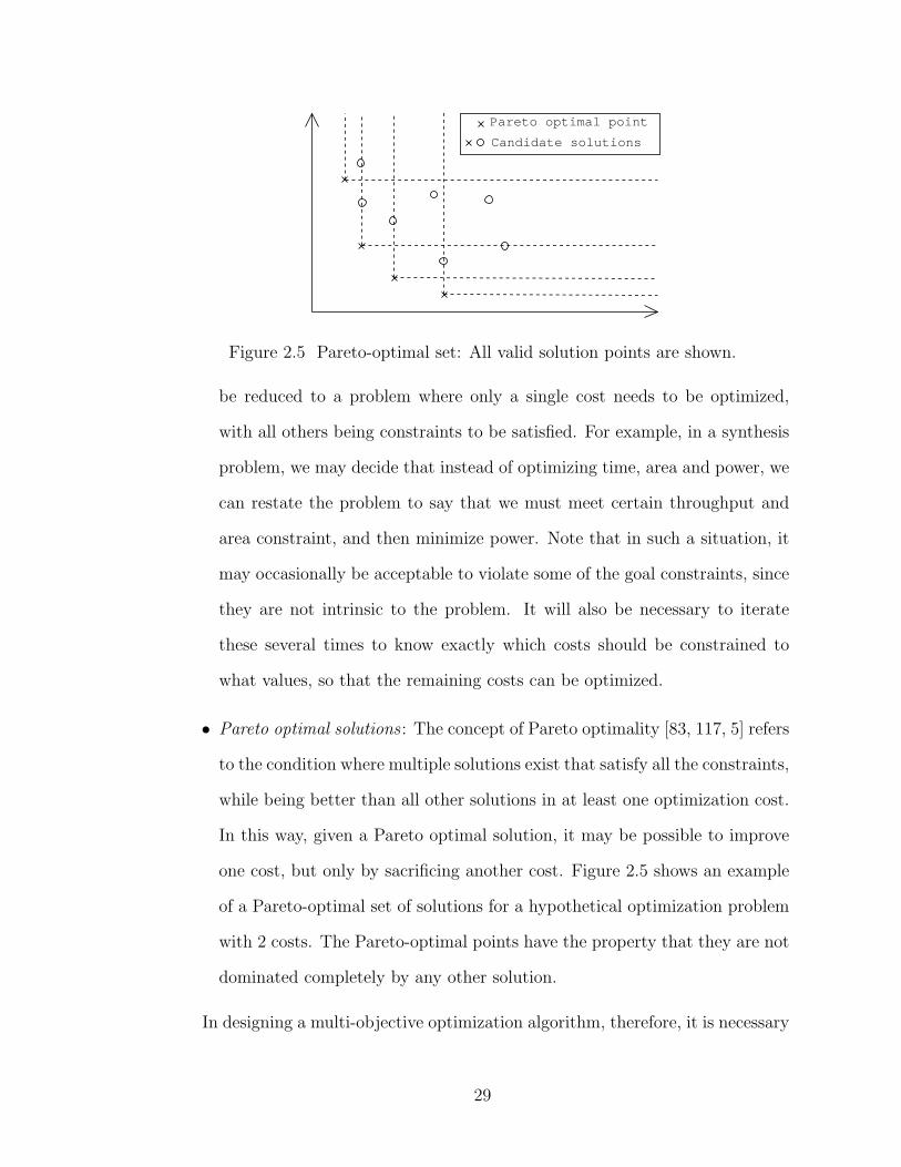
Figure 2.5 Pareto-optimal set: All valid solution points are shown.
be reduced to a problem where only a single cost needs to be optimized,
with all others being constraints to be satisfied. For example, in a synthesis
problem, we may decide that instead of optimizing time, area and power, we
can restate the problem to say that we must meet certain throughput and
area constraint, and then minimize power. Note that in such a situation, it
may occasionally be acceptable to violate some of the goal constraints, since
they are not intrinsic to the problem. It will also be necessary to iterate
these several times to know exactly which costs should be constrained to
what values, so that the remaining costs can be optimized.
• Pareto optimal solutions : The concept of Pareto optimality [83, 117, 5] refers
to the condition where multiple solutions exist that satisfy all the constraints,
while being better than all other solutions in at least one optimization cost.
In this way, given a Pareto optimal solution, it may be possible to improve
one cost, but only by sacrificing another cost. Figure 2.5 shows an example
of a Pareto-optimal set of solutions for a hypothetical optimization problem
with 2 costs. The Pareto-optimal points have the property that they are not
dominated completely by any other solution.
In designing a multi-objective optimization algorithm, therefore, it is necessary
29
to decide which of the different kinds of optimization we are looking for. In
addition, it is usually beneficial to have an algorithm that can generate multiple
Pareto-optimal points, so that a system designer can make an informed decision
as to which design point is the best, and locate potential tradeoffs.
Because evolutionary algorithms work on populations of candidate solutions, it
is natural for them to generate an entire set of Pareto-optimal solutions. Although
the solutions generated in each stage may not be truly optimal, it is still easy to
maintain a set of solutions that are currently the best, and in this way form an
efficient approximation of the true Pareto front.
Deterministic algorithms that generate Pareto fronts are relatively rare, since
the idea of a deterministic algorithm (following a specific sequence of steps in search
of an optimum) does not easily lend itself to finding several optimal solutions
simultaneously. Other randomized algorithms like simulated annealing and hill
climbing may also be able to generate Pareto optimal solutions, but since they are
usually working with a single candidate solution that they are trying to improve,
this is not as efficient as in evolutionary algorithms.
2.3 Complexity of the synthesis problem
The high level design process mostly concerns itself with the problems of
finding suitable description techniques (dataflow graph models [66, 17], hardware
description languages [59, 110], state machine descriptions [103, 37]), followed by
the three problems described above (allocation, binding and scheduling). The
primary difficulty in all approaches to these problems is caused by the fact that
the problems are computationally very complex: to be precise, they all fall in the
category of computational problems known as NP-Complete problems.
30
An algorithm or computational procedure [47, 32] is considered to be
“tractable” or useful if the running time of the algorithm is related to the size
of the input of the problem by some polynomial function. If, however, the running
time grows exponentially with the size of the input, then the algorithm cannot
usefully be applied to anything other than small instances of the problem.
The main property of NP-complete problems that is of relevant to our
discussion is the fact that there are no known techniques to solve these problems in
polynomial times. In addition, if such a method is ever found for any one of these
problems, it will become possible to solve all NP-complete problems in polynomial
techniques through a process of transforming problems from one kind to another.
There is considerable empirical evidence based on several years of research to
indicate that it may never be possible to find such a technique. Therefore NP-
complete problems are usually considered to be “hard” to solve exactly, and once
a problem is shown to be NP-complete, it is usually advisable to look for suitable
approximate or heuristic techniques to attack it.
The high level synthesis problems of allocation, binding and scheduling are
known to be NP-complete [36, 37] for all non-trivial sets of problems and resource
sets. As a result, it is not expected that a polynomial time solution will be found
for these problems.
In this situation, there are a number of approaches that can be taken to try
and obtain suitable solutions. These are outlined in the following sections.
2.3.1 Exact solution techniques
The first technique that can be considered to solve the synthesis problem is to try
for an exact solution technique. As discussed in [47], this is possible, but will in
general be so computationally expensive that it is not viable for anything other
31

than small problem instances. However, this may still be useful if it is known in
advance that the problem instances of interest are going to be small, or if we have
a suitably large computing facility to handle the problem size under consideration.
There are a few methods by which this process can be undertaken:
• Exhaustive search: In this, all possible combinations of resources and
mappings are explored to find the best solution. It may be possible to
improve the efficiency of the search process by using techniques such as
branch-and-bound and other tree pruning techniques to reduce the size of
the search space. An approach along these lines was proposed to solve the
cyclostatic processor scheduling problem in [102].
• Integer Linear Programming (ILP): This is an approach where we try to cast
the problem as a mathematical program of linear constraints [39, 68] where
the solution is required to take integer values. The ILP problem [58] is known
to be NP-complete in itself, so this does not actually present an improvement
in the solution technique. On the other hand, good approximate solutions
can sometimes be obtained through linear programming [33, 82], and there
are certain well known software packages that may be used to try and
efficiently solve the problem.
These techniques are mainly of interest for the purpose of comparing the results
that can be obtained using other techniques, on small benchmark examples. Also,
even though they solve the stated problem exactly, it may not be possible to
capture all constraints in the system in the description, so the extra effort of
attempting an exact solution may not be worth it.
32
2.3.2 Approximation algorithms
Although all NP-complete problems have the same asymptotic worst case
complexity bounds, it is often the case that particular formulations may be much
more amenable to approximate solutions [82]. In this way, several problems in
computer science such as the traveling salesman problem [96] and the knapsack
problem [65] have approximate solution techniques. These techniques are more
than just an inexact solution, they actually guarantee that the solution will be
within a certain multiplicative or additive bound of the ideal solution. In this
sense, they can be fairly tight bounds on the actual solutions.
Approximation algorithms are more difficult to develop and analyze fully than
general heuristics, and in several cases, the extra guarantee of being within a
certain multiplicative bound of the ideal solution is not particularly necessary to
have. Therefore it is much more common, especially in the problems related to
EDA, to find heuristic and randomized algorithms that do not provide performance
guarantees.
2.3.3 Heuristics
In the absence of exact solutions to the synthesis problems, it becomes necessary
to consider alternative approaches. One of the main categories of methods are
“heuristic techniques”, which are techniques based on experimental observations
or feedback from other attempts to solve similar problems.
For the problems in high level synthesis, one way of approaching the design
problem is to start by making a suitable allocation of resources and binding the
functions to resources. After this, the operations can be scheduled, and if the
constraints or costs are not satisfied, we can change the allocation to try and
33

improve the result. This division into distinct stages makes it possible to study
each problem separately, possibly coming up with better algorithms for each stage.
The disadvantage is that the overall holistic view of the system is lost, and it is
possible that certain good solutions are completely lost from consideration as a
result of this.
One of the most popular heuristics for the scheduling problem is based on the
idea of “priority based list scheduling” [37, 86]. The idea here is to rank all the
operations in the algorithm in terms of a certain priority weighting, and then use
this to decide which function is to be scheduled earlier than others. This is an
intuitively appealing technique, as we can use the dependency structure of the
problem graph to guide the scheduling. One of the simple choices for the priority
level is just the number of stages following a given node in a dataflow graph. In
this way, nodes that have many successors depending on them will tend to be
scheduled earlier, thereby ensuring a reasonably efficient ordering of functions. A
number of variations on this basic theme have been proposed that try to overcome
shortcomings in the basic method, and make it possible to adapt this algorithm
to other situations where the costs are different.
In most of the heuristic approaches, the allocation and binding are usually
done based on other heuristics, with the possibility of using feedback information
from the final schedule to improve the binding that is initially used [86, 24]. For
example, simple heuristics may try to allocate fast resources initially, and then
if the timing constraints are met easily, a few of the resources are replaced by
other resources that may consume less power or have lower costs. An overview of
the methods used by several different synthesis tools for this process is presented
in [86].
Most heuristics do not provide performance guarantees, so it is possible that
34
the solution produced by a heuristic is very bad indeed. Usually, though, most
problem graphs representing circuits tend to be well-behaved circuits, and well
designed heuristics have been able to provide reasonably good solutions for most
problems.
The main disadvantage of these techniques (apart from the fact that they do
not give exact solutions) is that when implemented as deterministic algorithms,
they can produce only a single solution, and it is not always obvious how to
use a given solution to obtain a better solution. In the current environment where
computing power is available to allow exploration of much larger design spaces, it is
desirable to have alternative techniques that are not restricted to such straight-line
designs. This is the main motivation behind using randomized and evolutionary
algorithms: these are techniques that introduce an element of randomness into
the search process, with the hope that they will be able to explore regions of the
search space that would normally be missed.
Some studies of the relative performances of different heuristic and randomized
approaches have been conducted, usually for distributed computing systems.
These systems are very similar to the parallel dataflow graphs we consider, but
have differences in the underlying architectures, and the focus is often more on
communication costs. Examples of such studies are [14, 4].
2.3.4 Randomized approaches
Non-exact approaches to the synthesis problem can therefore be of two kinds:
deterministic and random. In deterministic approaches, as discussed above, we go
through a well defined procedure that results in generation of a valid architecture
and schedule of operations. The main disadvantage of following this procedure is
that, owing to the highly irregular nature of the solution space, it is possible that
35
certain solutions will never be explored by the search algorithm.
As explained in sec. 2.2, the design space of architecture synthesis problems is
usually very complex. In general, deterministic approaches tend to follow certain
trajectories through this design space, possibly continuously moving to points
with better costs. However, to reach an optimal cost point, it may occasionally be
necessary to go through a path that temporarily worsens the cost of the design.
Most deterministic procedures cannot afford to look more than one or two stages
ahead in this search, because otherwise the complexity of the search will become
too high.
An alternative approach is to randomize the search. While completely random
algorithms (that randomly generate candidate solutions and evaluate them) have
a very low chance of actually obtaining good solutions, a much more promising
approach is to use a deterministic algorithm, but to supplement it with the
possibility of accepting some solutions that temporarily worsen the solution, in
the hope that it will later improve still further.
Examples of these randomized search techniques include simulated annealing,
Tabu search and Evolutionary algorithms. In each of these cases, different
approaches are used to guide the search along different parts of the design space,
in such a way as to result in a net improvement of the result, while also searching
as much of the space as possible. Simulated annealing and Tabu search both try
to improve existing solutions by modifying certain parameters and re-evaluating
them. They then use certain criteria to decide which of the modified solutions
may be accepted, and also to determine the path in the search space that is to be
followed.
36
2.3.5 Evolutionary algorithms
Evolutionary algorithms or EAs [52, 116, 7] offer an approach that is able to
encompass a very wide range of optimization problems, and have been shown over
several years to be a very suitable optimization technique in a number of situations.
The algorithms are inspired by the biological idea of evolution. A population of
sample solutions is generated randomly, and evaluated for their “fitness” for a
particular function. Based on this, and using the ideas of crossover, mutation and
selection of the fittest, these algorithms then try to improve the existing pool of
solution candidates.
There are several different approaches to evolutionary computation, of which
genetic algorithms (GA) [52] are probably the best known. They are characterized
by the use of “chromosomes” and a genotype-phenotype mapping to represent and
handle solution candidates.
The evolutionary algorithms are very popular because of their demonstrated
efficiency at handling a wide variety of problems. In addition, they also lend
themselves to efficient parallel implementation, and there exist well-tuned software
libraries that can be used for these algorithms.
An additional area where evolutionary algorithms are useful is in the area of
multi-objective optimization. In this problem, it is required to find a Pareto front
or set of Pareto points [117] instead of a unique optimum solution. For example,
we could have a design where we want to optimize both area and power. Using
a suitable multi-objective optimization system, it may be possible to generate a
number of solutions, and pick one of them for the actual implementation.
EAs have a number of drawbacks as well: although their general purpose
nature makes them well suited to several different types of tasks, this also means
37

that it is difficult for them to make good use of problem-specific knowledge that
might potentially lead to faster discovery of certain good solutions. Another big
problem with EAs is that their effectiveness is determined by the representation
used to encode the chromosomes. In several kinds of problems, notably in problems
involving sequences, such as scheduling, it is difficult to find a good representation
that fits the requirements directly [50]. This is in contrast to the use of EAs for
clustering problems, where it has been found that it is possible to develop good
chromosomes for clustering GAs [62]. It is often necessary to resort to complicated
repair and validation mechanisms [108], and this can skew the structure of the
design space, leaving certain areas unexplored while other areas are much more
likely to be explored than would happen with an unbiased representation.
2.3.6 Efficient use of compilation time computing power
It is clear from the previous discussions that the overall problem of electronic
design automation consists of a set of problems of high computational complexity.
Even when heuristics and randomized techniques are used, the algorithms retain
a high level of complexity.
Another factor is that because of improvements in algorithms and technology,
designers would like to incorporate more and more features into their designs.
These designs are now possible because the amount of silicon (in terms of the
number of computational units or transistors) available for a given cost has been
increasing rapidly in agreement with Moore’s law – i.e. roughly doubling every
18 months. In todays markets, continuously improving the feature set and quality
of designs is the only way to remain competitive. For such complex designs, it
becomes almost impossible for a single person or even a small design group to
keep track of all factors in the design, and generate an optimum design.
38
On the other hand, the computational power that can be applied to solve the
design problems has also been growing rapidly over the past several years, in a
manner that agrees with Moore’s law. Given this factor, it becomes necessary to
consider design techniques that usefully exploit this increased computing power to
improve the designs and reduce the burden on the designer.
There are two ways of exploiting increases in computing power: one way is to
develop more efficient analysis and synthesis techniques, but in a way that benefits
from being given more time to run (examples include evolutionary techniques and
many probabilistic search methods). The other factor to be considered is the
possibility of breaking up a synthesis process into a number of smaller steps, and
then trying to come up with an optimal way of using these individual steps such
that the overall time allocated to compilation is used in the best way possible.
The ideas of anytime algorithms [38, 13] are one way in which this can be done.
This process is not considered in further detail in this thesis, where we concentrate
more on the first aspect, namely developing more efficient ways of analyzing system
performance and using these techniques to improve synthesis algorithms.
Evolutionary algorithms and other randomized algorithms are very useful for
this because they are able to continuously improve a set of candidate solutions.
In this way, it becomes possible to use relatively simple but fast algorithms to
explore large parts of the design space, and this can supplement a more focused
initial search by heuristics and human experience.
39
Chapter 3
Performance analysis in dynamic graphs
3.1 Introduction
In the previous chapter, we looked at the problem of high level synthesis (HLS)
and identified some areas that can lead to improved algorithms for design space
exploration. In this chapter, we look at one of the problems, namely performance
analysis. In the following sections, we will first look at why performance analysis
is a crucial part of design space exploration, and will also motivate the concept
of dynamic graphs. We then present the Adaptive Bellman Ford algorithm as a
suitable technique for solving the problems of feasibility analysis on a dynamic
graph, and provide application examples that show where such a system is useful.
3.2 Performance analysis and negative cycle detection
Once a dataflow graph (corresponding to the DSP algorithm to be implemented)
has been mapped onto a set of resources, its performance can be estimated in
terms of the execution times of each of the operations on the resources. The
execution model typically assumed is that each operation takes a fixed amount of
time depending on the exact resource type it is mapped to.
40
For acyclic graphs the goal is usually to minimize the makespan of the graph:
the total time for completion of all operations. This metric is primarily determined
by the execution times of operations on the longest (critical) path through the
graph, but may also need inter-processor communication costs to be taken into
account.
For cyclic graphs such as those underlying many DSP systems, the situation
is slightly different. In these graphs (also called iterative dataflow graphs [36]),
inter-iteration parallelism is much more important. That is, it is possible
that different resources are simultaneously executing operations corresponding to
different iterations of the input data stream. In the case where we have an acyclic
graph but we allow overlapped execution of different iterations, this can usually
be treated as a special case of a cyclic dataflow graph.
The primary difference between cyclic systems and acyclic systems lies in the
fact that the critical path (longest execution path from input to output) need not
be the determining factor of the throughput of the graph. The actual throughput
is now determined by a metric known as the maximum cycle mean [95, 60, 51].
This quantity corresponds in some sense to a longest cycle in the graph, rather
than a longest path. But an important difference is that the actual obtainable
throughput depends on the number of delays on this cycle. The main idea here
is that, if there is a directed cycle in the graph, we will have an impossible set
of dependencies, unless at least one of these edges has one or more delays on it.
The presence of a delay on an edge means that the vertex attached to the sink
of the edge is operating on data from a previous iteration, and this introduces
a slack of one time period into that cycle. Therefore, even if there is a single
path through the graph that corresponds to a very long chain of operations, it
is possible that the actual obtainable iteration period bound is much lower than
41
the sum of execution times on this path, as long as a sufficiently large number
of delay elements exist on this cycle. In terms of the weights of edges around a
cycle, the above requirement can be translated into a requirement that the sum of
the weights on edges around every cycle in the graph must be positive in order to
prevent an infeasible constraint. Therefore, a negative cycle, which is a directed
cycle with a total weight less than zero, indicates an impossible set of constraints.
The delay elements in a cyclic graph therefore play a very important role:
they are responsible for allowing the overlapped execution of multiple iterations of
the graph simultaneously. In graph representations such as SDF [66], the initial
tokens on edges are equivalent to delay elements. In clocked circuitry, the delay
elements correspond to registers [67, 42]. Registers in synchronous circuits are
usually treated as being triggered by a single globally synchronous clock, but it
has been recognized that manipulating the exact phase of the firing of a register
can allow the circuit to obtain either higher throughput or better safety margins
than using a single global clock phase [42, 97, 100]. This becomes possible because
manipulating these trigger phases changes the effective length of the longest path
between any two firings of registers in the circuit. By reducing this time, the
effective longest path through the circuit can be made shorter than the actual
longest path between two registers, thus providing some freedom to reduce the
clock period.
For the purpose of HLS, a common assumption regarding the operation of the
register elements is that they function as delays in a self-timed operation of the
circuit. That is, each element in the circuit waits until all its inputs are available,
and then executes. The output that is generated after some amount of time (the
execution time of the operation) is then made available to all vertices in the graph
that require this as their input. This is a self-timed mode of operation, and is
42
the most natural mode of execution of the operations when the start and end
times of the operations can be readily signaled from one to the other. Under these
assumptions, the execution times of operations set up a system of constraints on
the graph that can easily be checked for feasibility. In this scenario, the delay
elements also act as constraints, but differ from other execution times in that they
provide a negative constraint, to indicate the fact that the output side of the delay
element is working on data from an earlier iteration than the input side.
In addition to these problems from HLS, several other problems in circuits
and systems theory require the solving of constraint equations [29, 94, 35, 46, 70].
Examples include VLSI layout compaction, interactive (reactive) systems, graphic
layout heuristics, and timing analysis and retiming of circuits for performance
or area considerations. Though a general system of constraints would require a
linear programming (LP) approach [33] to solve it, several problems of interest
actually consist of the special case of difference constraints, where each constraint
expresses the minimum or maximum value that the difference of two variables in
the system can take. These problems can be attacked by faster techniques than
the general LP [94, 32], mostly involving the solution of a shortest path problem on
a weighted directed graph. Detection of negative cycles in the graph is therefore a
closely related problem, as it would indicate in-feasibility of the constraint system.
Because of the above reasons, detecting the presence of negative cycles in a
weighted directed graph is a very important problem in systems theory. This
problem is also important in the computation of network flows. Considerable
effort has been spent on finding efficient algorithms for this purpose. Cherkassky
and Goldberg [29] have performed a comprehensive survey of existing techniques.
Their study shows some interesting features of the available algorithms, such as
the fact that for a large class of random graphs, the worst case performance bound
43

is far more pessimistic than the observed performance.
There are also situations in which it is useful or necessary to maintain a feasible
solution to a set of difference constraints as a system evolves. Typical examples
of this would be real-time or interactive systems, where constraints are added or
removed one (or several) at a time, and after each such modification it is required
to determine whether the resulting system has a feasible solution and if so, to find
it. In these situations, it may be more efficient to adapt existing information to aid
the solution of the constraint system, than to use the normal approach of applying
the solution technique to the new problem starting from scratch. In the example
from HLS that was mentioned previously, it is possible to cast the problem of
design space exploration in a way that benefits from this approach.
Several researchers [92, 46, 2] have worked on the area of incremental
computation. They have presented analyses of algorithms for the shortest path
problem and negative cycle detection in dynamic graphs. Most of the approaches
try to apply modifications of Dijkstra’s algorithm [32, p.527] to the problem. The
obvious reason for this is that this is the fastest known algorithm for the problem
when only positive weights are allowed on edges. However, use of Dijkstra’s
algorithm as the basis for incremental computation requires the changes to be
handled one at a time. While this may often be efficient enough, there are many
cases where the ability to handle multiple changes simultaneously would be more
advantageous. For example, it is possible that in a sequence of changes, one
reverses the effect of another: in this case, a normal incremental approach would
perform the same computation twice, while a delayed adaptive computation would
not waste any effort.
In this chapter, we consider an approach that generalizes the adaptive
approach beyond single increments: multiple changes to the graph are addressed
44
simultaneously. The approach can be applied to cases where it is possible to
collect several changes to the graph structure before updating the solution to the
constraint set. As mentioned previously, this can result in increased efficiency in
several important problems. Simulation results comparing this method against
the single-increment algorithm proposed in [94] are presented. For larger numbers
of changes, the algorithm presented here performs considerably better than this
incremental algorithm.
To illustrate the advantages of our adaptive approach, we present an
application from the area of HLS, namely the computation of the iteration period
bound [95] or maximum cycle mean of a dataflow graph. We show how the
negative cycle detection using the new Adaptive Bellman-Ford technique can be
used to derive a fast implementation of Lawler’s algorithm for the problem of
computing the maximum cycle mean (MCM) of a weighted directed graph. We
present experimental results comparing this against Howard’s algorithm [31, 35],
which appears to be the fastest algorithm available in practice. We find that for
graph sizes and node-degrees similar to those of real circuits, our algorithm often
outperforms even Howard’s algorithm.
In chapter 5, we will consider an approach to architecture synthesis that uses
negative cycle detection on dynamic graphs as an important core routine. The
results there show that this new approach based on the ABF algorithm can be
successfully used to speed up the design space exploration in this problem as well.
Section 3.3 surveys previous work on shortest path algorithms and incremental
algorithms. In Section 3.4, we describe the adaptive algorithm that works on
multiple changes to a graph efficiently. Section 3.5 compares our algorithm against
the existing approach, as well as against another possible candidate for adaptive
operation. Section 3.6 then gives details of the application of the adaptive negative
45
cycle detection to the problem of computing the MCM of a graph, and presents
some experimental results. Finally, we present our conclusions and examine areas
that would be suitable for further investigation.
A preliminary version of the results presented in this chapter were published
in [20].
3.3 Previous work
Cherkassky and Goldberg [29] have conducted an extensive survey of algorithms
for detecting negative cycles in graphs. They have also performed a similar study
on the problem of shortest path computations. They present several problem
families that can be used to test the effectiveness of a cycle-detection algorithm.
One surprising fact is that the best known theoretical bound (O(|V ||E|), where |V |is the number of vertices and |E| is the number of edges in the graph) for solving
the shortest path problem (with arbitrary weights) is also the best known time
bound for the negative-cycle problem. But examining the experimental results
from their work reveals the interesting fact that in almost all of the studied
samples, the performance is considerably less costly than would be suggested by
the product (|V | × |E|). It appears that the worst case is rarely encountered in
random examples, and an average case analysis of the algorithms might be more
useful.
Recently, there has been increased interest in the subject of dynamic or
incremental algorithms for solving problems [92, 2, 46]. This uses the fact that
in several problems where a graph algorithm such as shortest paths or transitive
closure needs to be solved, it is often the case that we need to repeatedly solve
the problem on variants of the original graph. The algorithms therefore store
46
information about the problem that was obtained during a previous iteration and
use this as an efficient starting point for the new problem instance corresponding
to the slightly altered graph. The concept of bounded incremental computation
introduced in [92] provides a framework within which the improvement afforded
by this approach can be quantified and analyzed.
In this chapter, the problem we are most interested in is that of maintaining
a solution to a set of difference constraints. This is equivalent to maintaining a
shortest path tree in a dynamic graph [94]. Frigioni et al. [46] present an algorithm
for maintaining shortest paths in arbitrary graphs that performs better than
starting from scratch, while Ramalingam and Reps [93] present a generalization of
the shortest path problem, and show how it can be used to handle the case where
there are few negative weight edges. In both of these cases, they have considered
one change at a time (not multiple changes), and the emphasis has been on the
theoretical time bound, rather than experimental analysis. In [45], the authors
present an experimental study, but only for the case of positive weight edges,
which restricts the study to computation of shortest paths and does not consider
negative weight cycles.
The most significant work along the lines we propose is described in [94]. In
this, the authors use the observation that in order to detect negative cycles, it is
not necessary to maintain a tree of the shortest paths to each vertex. They suggest
an improved algorithm based on Dijkstra’s algorithm, which is able to recompute a
feasible solution (or detect a negative cycle) in time O(E +V log V ), or in terms of
output complexity (defined and motivated in [94]) O(‖∆‖+ |∆| log |∆|), where|∆|is the number of variables whose values are changed and ‖∆‖ is the number of
constraints involving the variables whose values have changed.
The above problem can be generalized to allow multiple changes to the graph
47
between calls to the negative cycle detection algorithm. In this case, the above
algorithms would require the changes to be handled one at a time, and therefore
would take time proportional to the total number of changes. On the other hand,
it would be preferable if we could obtain a solution whose complexity depends
instead on the number of updates requested, rather than the total number of
changes applied to the graph. Multiple changes between updates to the negative
cycle computation arise naturally in many interactive environments, (e.g., if we
prefer to accumulate changes between refreshes of the state, using the idea of
lazy evaluation) or in design space-exploration, as can be seen, for example, in
section 5.1. By accumulating changes and processing them in large batches, we
remove a large overhead from the computation, which may result in considerably
faster algorithms.
Note that the work in [94] also considers the addition/deletion of constraints
only one at a time. It needs to be emphasized that this limitation is basic to the
design of the algorithm: Dijkstra’s algorithm can be applied only when the changes
are considered one at a time. This is acceptable in many contexts since Dijkstra’s
algorithm is the fastest algorithm for the case where edge weights are positive.
If we try using another shortest-paths algorithm we would incur a performance
penalty. However, as we show, this loss in performance in the case of unit changes
may be offset by improved performance when we consider multiple changes.
The approach we present for the solution is to extend the classical Bellman-
Ford algorithm for shortest paths in such a way that the solution obtained in one
problem instance can be used to reduce the complexity of the solution in modified
versions of the graph. In the incremental case (single changes to the graph) this
problem is related to the problem of analyzing the “sensitivity” of the algorithm [1].
The sensitivity analysis tries to study the performance of an algorithm when its
48
inputs are slightly perturbed. Note that there do not appear to be any average case
sensitivity analyses of the Bellman-Ford algorithm, and the approach presented
in [1] has a quadratic running time in the size of the graph. This analysis is
performed for a general graph without regard to any special properties it may
have. But as explained in sec. 3.6.1, graphs corresponding to circuits and systems
in HLS for DSP are typically very sparse – most benchmark graphs tend to have
a ratio of about 2 edges per vertex, and the number of delay elements is also small
relative to the total number of vertices. Our experiments have shown that in these
cases, the adaptive approach is able to do much better than a quadratic approach.
We also provide application examples to show other potential uses of the approach.
In the following sections, we show that our approach performs almost as well
as the approach in [94] (experimentally) for changes made one at a time, and
significantly outperforms their approach under the general case of multiple changes
(this is true even for relatively small batches of changes, as will be seen from the
results). Also, when the number of changes between updates is very large, our
algorithm reduces to the normal Bellman-Ford algorithm (starting from scratch),
so we do not lose in performance. This is important since when a large number of
changes are made, the problem can be viewed as one of solving the shortest-path
problem for a new graph instance, and we should not perform worse than the
standard available technique for that.
Our interest in adaptive negative cycle detection stems primarily from its
application in the problems of HLS that we outlined in the previous section. To
demonstrate its usefulness in these areas, we have used this technique to obtain
improved implementations of the performance estimation problem (computation of
the MCM) and to implement an iterative improvement technique for design space
exploration. Dasdan et al. [35] present an extensive study of existing algorithms for
49
computing the MCM. They conclude that the most efficient algorithm in practice
is Howard’s algorithm [31]. We show that the well known Lawler’s algorithm [64],
when implemented using an efficient negative-cycle detection technique and with
the added benefit of our adaptive negative cycle detection approach, actually
outperforms this algorithm for several test cases, including several of the ISCAS
benchmarks, which represent reasonable sized circuits.
As mentioned previously, the relevance of negative cycle detection to design
space exploration is because of the cyclic nature of the graphs for DSP applications.
That is, there is often a dependence between the computation in one iteration
and the values computed in previous iterations. Such graphs are referred to
as “Iterative dataflow graphs” [36]. Traditional scheduling techniques tend to
consider only the latency of the system, converting it to an acyclic graph if
necessary. This can result in loss of the ability to exploit inter-iteration parallelism
effectively. Methods such as “Optimum unfolding” [84] and “Range-chart guided
scheduling” [36] are techniques that try to avoid this loss in potential parallelism by
working directly on the cyclic graph. However, they suffer from some disadvantages
of their own. Optimum unfolding can potentially lead to a large increase in the
size of the resulting graph to be scheduled. Range chart guided scheduling is a
deterministic heuristic that could miss potential solutions. In addition, the process
of scanning through all possible time intervals for scheduling an operation can work
only when the run-times of operations are small integers. This is more suited to
a software implementation than a general hardware design. These techniques
also work only after a function to resource binding is known, as they require
timing information for the functions in order to schedule them. For the general
architecture synthesis problem, this binding itself needs to be found through a
search procedure, so it is reasonable to consider alternate search schemes that
50
combine the search for architecture with the search for a schedule.
If the cyclic dataflow graph is used to construct a constraint graph, then
feasibility of the resulting system is determined by the absence of negative cycles
in the graph. This can be used to obtain exact schedules capable of attaining the
performance bound for a given function to resource binding. For the problem of
design space exploration, we treat the problem of scheduling an iterative dataflow
graph (IDFG) as a problem of searching for an efficient ordering of function vertices
on processors, which can be treated as addition of several timing constraints to an
existing set of constraints. We implement a simple search technique that uses this
approach to solve a number of scheduling problems, including scheduling for low-
power on multiple-voltage resources, and scheduling on homogeneous processors,
within a single framework. The advantages of using iterative improvement
search techniques for design space exploration is motivated by the fact that it
is not possible to provide deterministic algorithms to exactly solve the scheduling
problem. Previous approaches, such as in [90], have proposed a search technique
using a sequence of moves, where they use an internal scheduling algorithm to
actually perform the ordering of operations. Our approach differs from this in that
we use a simple technique for negative cycle detection as the core of the algorithm.
Since the feasibility analysis forms the core of the search, speeding this up should
result in a proportionate increase in the number of designs evaluated (until such
a point that this is no longer the bottleneck in the overall computation). The
adaptive negative cycle detection technique ensures that we can do such searches
efficiently, by restricting the computations required. The results of developing an
algorithm based on this principle is presented, together with comparisons against
some other architectural synthesis algorithms, in section 5.1.
51
3.4 The Adaptive Bellman-Ford Algorithm
In this section, we present the basis of the adaptive approach that enables efficient
detection of negative cycles in dynamic graphs. This is equivalent to the problem
of deciding whether a given set of difference constraints has a feasible solution.
The conversion between these two points of view is explained below.
Observe that if we have a set of difference constraints of the form
xi − xj ≤ bij
we can construct a digraph with vertices corresponding to xi, and an edge (eij)
directed from the vertex corresponding to xi to the vertex for xj such that
weight(eij) = bij . This procedure is performed for each constraint in the system
and a weighted directed graph is obtained. Solving for shortest paths in this graph
would yield a set of distances dist that satisfy the constraints on xi. This graph
is henceforth referred to as the constraint graph.
The usual technique used to solve for dist is to introduce an imaginary vertex
s0 to act as a (pseudo) source, and introduce edges of zero-weight from this vertex
to each of the other vertices. The resulting graph is referred to as the augmented
graph [94]. In this way, we can use a single-source shortest paths algorithm to find
dist from s0, and any negative cycles (infeasible solution) found in the augmented
graph must also be present in the original graph, since the new vertex and edges
cannot create cycles.
The Bellman-Ford-Moore algorithm for shortest paths (independently
proposed by R. E. Bellman [8], L. Ford [44] and E. F. Moore [78]) is an application
of the principle of dynamic programming to the problem of finding shortest paths
in a network. It is often referred to in the literature as the Bellman-Ford algorithm.
This algorithm is capable of finding the shortest path between a source and sink
52
vertex in a graph under any weight distribution.
The basic Bellman-Ford algorithm does not provide a standard way of detecting
negative cycles in the graph. However, it is obvious from the way the algorithm
operates that if changes in the distance labels continue to occur for more than a
certain number of iterations, there must be a negative cycle in the graph. This
observation has been used to detect negative cycles, and with this straightforward
implementation, we obtain an algorithm to detect negative cycles that takes
O(|V |3) time, where |V | is the number of vertices in the graph.
The study by Cherkassky and Goldberg [29] presents several variants of the
negative cycle detection technique. The technique they found to be most efficient in
practice is based on the “subtree disassembly” technique proposed by Tarjan [107].
This algorithm works by constructing a shortest path tree as it proceeds from the
source of the problem, and any negative cycle in the graph will first manifest itself
as a violation of the tree order in the construction. The experimental evaluation
presented in their study found this algorithm to be a robust variant for the negative
cycle detection problem. As a result of their findings, we have chosen this algorithm
as the basis for the adaptive algorithm. Our modified algorithm is henceforth
referred to as the “Adaptive Bellman-Ford (ABF)” algorithm.
The adaptive version of the Bellman-Ford algorithm works on the basis of
storing the distance labels that were computed from the source vertex from one
iteration to the next. Since the negative cycle detection problem requires that
the source vertex is always the same (the augmenting vertex), it is intuitive that
as long as most edge weights do not change, the distance labels for most of the
vertices will also remain the same. Therefore, by storing this information and
using it as a starting point for the negative cycle detection routines, we can save
a considerable amount of computation.
53
One possible objection to this system is that we would need to scan all the edges
each time in order to detect vertices that have been affected. In several applications
involving multiple changes to a graph, it is possible to pass information to the
algorithm about which vertices have been affected. This information can be
generated by the higher level application-specific process making the modifications.
For example, if we consider multiprocessor scheduling, the high-level process would
generate a new vertex ordering, and add edges to the graph to represent the new
constraints. Since any changes to the graph can only occur at these edges, the
application can pass on to the ABF algorithm precise information about what
changes have been made to the graph, thus saving the trouble of scanning the
graph for changes.
Note that in the event where the high-level application cannot pass on this
information without adding significant bookkeeping overhead, the additional work
required for a scan of the edges is proportional to the number of edges, and hence
does not affect the overall complexity, which is at least as large as this. For
example, in the case of the maximum cycle mean computation examined below,
for most circuit graphs the number of edges with delays is about 1/10 as many as
the total number of edges. With each change in the target iteration period, most
of these edges will cause constraint violations. In such a situation, an edge scan
provides a way of detecting violations that is very fast and easy to implement,
while not increasing the overall complexity of the method.
3.4.1 Correctness of the method
The use of a shortest path routine to find a solution to a system of difference
constraint equations is based on the following two theorems, which are not hard
to prove (see [32]).
54
Theorem 3.1 A system of difference constraints is consistent if and only if its
augmented constraint graph has no negative cycles, and the latter condition holds
if and only if the original constraint graph has no negative cycles.
Theorem 3.2 Let G be the augmented constraint graph of a consistent system of
constraints 〈V, C〉. Then D is a feasible solution for 〈V, C〉, where
D(u) = distG(s0, u)
In Theorem 3.2, the constraint graph is defined as in sec. 3.4 above. The
augmented constraint graph consists of this graph, together with an additional
source vertex (s0) that has 0-weight edges leading to all the other existing vertices,
and consistency means that a set of xi exist that satisfy all the constraints in the
system.
In the adaptive version of the algorithm, we are effectively setting the weights of
the augmenting edges to be equal to the labels that were computed in the previous
iteration. In this way, the initial scan from the augmenting vertex sets the distance
label at each vertex equal to the previously computed weight instead of setting
it to 0. So we now need to show that using non-zero weights on the augmenting
edges does not change the solution space in any way: i.e. all possible solutions for
the 0-weight problem are also solutions for the non-zero weight problem, except
possibly for translation by a constant.
The new algorithm with the adaptation enhancements can be seen to be correct
if we relax the definition of the augmented graph so that the augmenting edges
(from s0) need not have 0 weight. We summarize the arguments for this in the
following theorems:
55
Theorem 3.3 Consider a constraint graph augmented with a source vertex s0,
and edges from this vertex to every other vertex v, such that these augmenting
edges have arbitrary weights. The associated system of constraints is consistent if
and only if the augmenting graph defined above has no negative cycles, which in
turn holds if and only if the original constraint graph has no negative cycles.
Proof: Clearly, since s0 does not have any in-edges, no cycles can pass through
it. So any cycles, negative or otherwise, which are detected in the augmented
graph, must have come from the original constraint graph, which in turn would
happen only if the constraint system was inconsistent (by Theorem 3.1). Also, any
inconsistency in the original system would manifest itself as a negative cycle in
the constraint graph, and the above augmentation cannot remove any such cycle.
2
The following theorem establishes the validity of solutions computed by the
ABF algorithm.
Theorem 3.4 If G′ is the augmented graph with arbitrary weights as defined
above, and D(u) = distG′(s0, u) (shortest paths from s0), then
1. D is a solution to 〈V, C〉; and
2. Any solution to 〈V, C〉 can be converted into a solution to the constraint
system represented by G′ by adding a constant to D(u) for each u ∈ V .
Proof: The first part is obvious, by the definition of shortest paths.
Now we need to show that by augmenting the graph with arbitrary weight
edges, we do not prevent certain solutions from being found. To see this, first
note that any solution to a difference constraint system remains a solution when
56
translated by a constant. That is, we can add or subtract a constant to all the
D(u) without changing the validity of the solution.
In our case, if we have a solution to the constraint system that does not satisfy
the constraints posed by our augmented graph, it is clear that the constraint
violation can only be on one of the augmenting edges (since the underlying
constraint graph is the same as in the case where the augmenting edges had zero
weight). Therefore, if we define
lmax = max{weight(e)|e ∈ Sa},
where Sa is the set of augmenting edges and
D′(u) = D(u)− lmax,
we ensure that D′ satisfies all the constraints of the original graph, as well as all
the constraints on the augmenting edges. 2
Theorem 3.4 tells us that an augmented constraint graph with arbitrary weights
on the augmenting edges can also be used to find a feasible solution to a constraint
system. This means that once we have found a solution dist : V →R (where R is
the set of real numbers) to the constraint system, we can change the augmented
graph so that the weight on each edge e : u → v is dist(v). Now even if we change
the underlying constraint graph in any way, we can use the same augmented graph
to test the consistency of the new system.
Figure 3.1 helps to illustrate the concepts that are explained in the previous
paragraphs. In part (B) of the figure, there is a change in the weight of one
edge. But as we can see from the augmented graph, this will result in only the
single update to the affected vertex itself, and all the other vertices will get their
constraint satisfying values directly from the previous iteration.
57
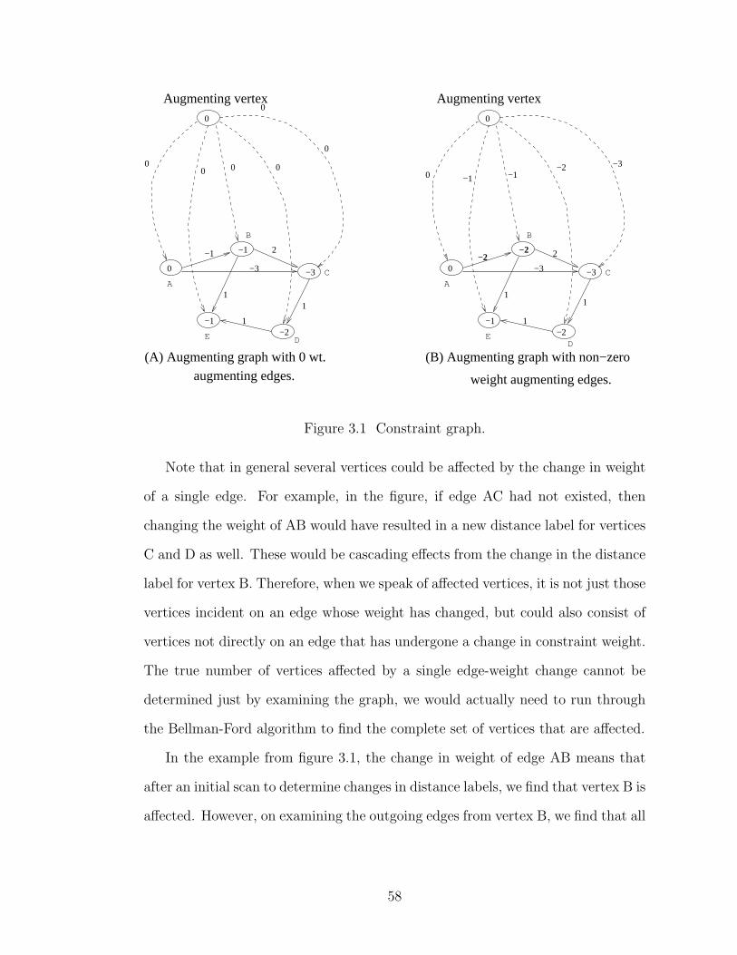
(A) Augmenting graph with 0 wt. augmenting edges.
(B) Augmenting graph with non−zero
weight augmenting edges.
Augmenting vertex Augmenting vertex 0
0
0000
−1 2
−3
1
1
1
0
−1
−3
−2−1
0 0
0 −1 −1−2 −3
0
−1 1
1
−2
−3−3
2
1
−2−2
A
B
C
DE
A
B
C
DE
Figure 3.1 Constraint graph.
Note that in general several vertices could be affected by the change in weight
of a single edge. For example, in the figure, if edge AC had not existed, then
changing the weight of AB would have resulted in a new distance label for vertices
C and D as well. These would be cascading effects from the change in the distance
label for vertex B. Therefore, when we speak of affected vertices, it is not just those
vertices incident on an edge whose weight has changed, but could also consist of
vertices not directly on an edge that has undergone a change in constraint weight.
The true number of vertices affected by a single edge-weight change cannot be
determined just by examining the graph, we would actually need to run through
the Bellman-Ford algorithm to find the complete set of vertices that are affected.
In the example from figure 3.1, the change in weight of edge AB means that
after an initial scan to determine changes in distance labels, we find that vertex B is
affected. However, on examining the outgoing edges from vertex B, we find that all
58
other constraints are satisfied, so the Bellman-Ford algorithm can terminate here
without proceeding to examine all other edges. Therefore, in this case, there is only
1 vertex whose label is affected out of the 5 vertices in the graph. Furthermore, the
experiments show that even in large sparse graphs, the effect of any single change
is usually localized to a small region of the graph, and this is the main reason that
the adaptive approach is useful, as opposed to other techniques that are developed
for more general graphs. Note that, as explained in the previous section, the initial
overhead for detecting constraint violations still holds, but the complexity of this
operation is significantly less than that of the Bellman-Ford algorithm.
3.5 Comparison against other incremental algorithms
The motivation for studying incremental and dynamic algorithms (that maintain
state information to speed up future computations) is because there occur actual
practical situations where a solution to a set of constraints or other similar problem
needs to be maintained in the face of repeated changes to the underlying system. In
the case of incremental algorithms, such as the ideas in [94, 2, 45], the assumption
is that changes to the underlying system (graph) are made one edge at a time.
This allows the use of algorithms tuned for this particular special case.
As discussed in the introduction of this chapter, we may often encounter
situations where the changes to the graph are made in batches of size greater
than 1. In this situation, incremental algorithms need to be invoked repeatedly
for each edge, thus incurring large overheads.
The proposed ABF algorithm is meant to tackle the problem of multiple
changes, and provide a better method for handling multiple changes to the graph
in a single invocation. Therefore, the comparative study that follows is aimed at
59
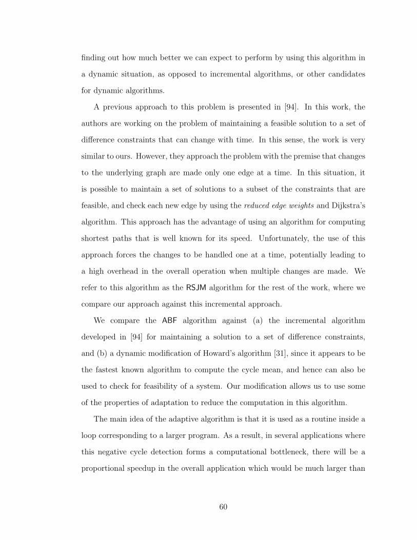
finding out how much better we can expect to perform by using this algorithm in
a dynamic situation, as opposed to incremental algorithms, or other candidates
for dynamic algorithms.
A previous approach to this problem is presented in [94]. In this work, the
authors are working on the problem of maintaining a feasible solution to a set of
difference constraints that can change with time. In this sense, the work is very
similar to ours. However, they approach the problem with the premise that changes
to the underlying graph are made only one edge at a time. In this situation, it
is possible to maintain a set of solutions to a subset of the constraints that are
feasible, and check each new edge by using the reduced edge weights and Dijkstra’s
algorithm. This approach has the advantage of using an algorithm for computing
shortest paths that is well known for its speed. Unfortunately, the use of this
approach forces the changes to be handled one at a time, potentially leading to
a high overhead in the overall operation when multiple changes are made. We
refer to this algorithm as the RSJM algorithm for the rest of the work, where we
compare our approach against this incremental approach.
We compare the ABF algorithm against (a) the incremental algorithm
developed in [94] for maintaining a solution to a set of difference constraints,
and (b) a dynamic modification of Howard’s algorithm [31], since it appears to be
the fastest known algorithm to compute the cycle mean, and hence can also be
used to check for feasibility of a system. Our modification allows us to use some
of the properties of adaptation to reduce the computation in this algorithm.
The main idea of the adaptive algorithm is that it is used as a routine inside a
loop corresponding to a larger program. As a result, in several applications where
this negative cycle detection forms a computational bottleneck, there will be a
proportional speedup in the overall application which would be much larger than
60
the speedup in a single run.
It is worth making a couple of observations at this point regarding the
algorithms we compare against.
1. The RSJM algorithm [94] uses Dijkstra’s algorithm as the core routine
for quickly recomputing the shortest paths. Using the Bellman-Ford
algorithm here (even with Tarjan’s implementation) would result in a loss in
performance since it cannot match the performance of Dijkstra’s algorithm
when edge weights are positive. Consequently, no benefit would be derived
from the reduced-cost concept used in [94].
2. The code for Howard’s algorithm was obtained from the Internet web-site
of the authors of [31]. The modifications suggested by Dasdan et al. [34]
have been taken into account by the original authors, and the code available
from their web-site incorporates these changes. This method of constraint
checking uses Howard’s algorithm to see if the MCM of the system yields a
feasible value, otherwise the system is deemed inconsistent.
Another important point is the type of graphs on which we have tested the
algorithms. We have restricted our attention to sparse graphs, or bounded degree
graphs. In particular, we have tried to keep the vertex-to-edge ratio similar to
what we may find in practice, as in, for example, the ISCAS benchmarks [15].
To understand why such graphs are relevant, note the following two points about
the structural elements usually found in circuits and signal processing blocks: (a)
they typically have a small, finite number of inputs and outputs (e.g. AND gates,
adders, etc. are binary elements) and (b) the fanout that is allowed in these
systems is usually limited for reasons of signal strength preservation (buffers are
used if necessary). For these reasons, the graphs representing practical circuits can
61
be well approximated by bounded degree graphs. In more general DSP application
graphs, constraints such as fanout may be ignored, but the modular nature of these
systems (they are built up of simpler, small modules) implies that they normally
have small vertex degrees.
We have implemented all the algorithms under the LEDA [75] framework for
uniformity. The tests were run on random graphs, with several random variations
performed on them thereafter. We kept the number of vertices constant and
changed only the edges. This was done for the following reason: a change to a
node (addition/deletion) may result in several edges being affected. In general,
due to the random nature of the graph, we cannot know in advance the exact
number of altered edges. Therefore, in order to keep track of the exact number
of changes, we applied changes only to the edges. Note that when node changes
are allowed, the argument for an adaptive algorithm capable of handling multiple
changes naturally becomes stronger.
In the discussion that follows, we use the term “batch-size” to refer to the
number of changes in a multiple change update. That is, when we make multiple
changes to a graph between updates, the changes are treated as a single batch,
and the actual number of changes that was made is referred to as the batch-size.
This is a useful parameter to understand the performance of the algorithms.
The changes that were applied to the graph were of 3 types:
• Edge insertion: An edge is inserted into the graph, ensuring that multiple
edges between vertices do not occur.
• Edge deletions: An edge is chosen at random and deleted from the graph.
Note that, in general, this cannot cause any violations of constraints.
• Edge weight change: An edge is chosen at random and its weight is changed
62
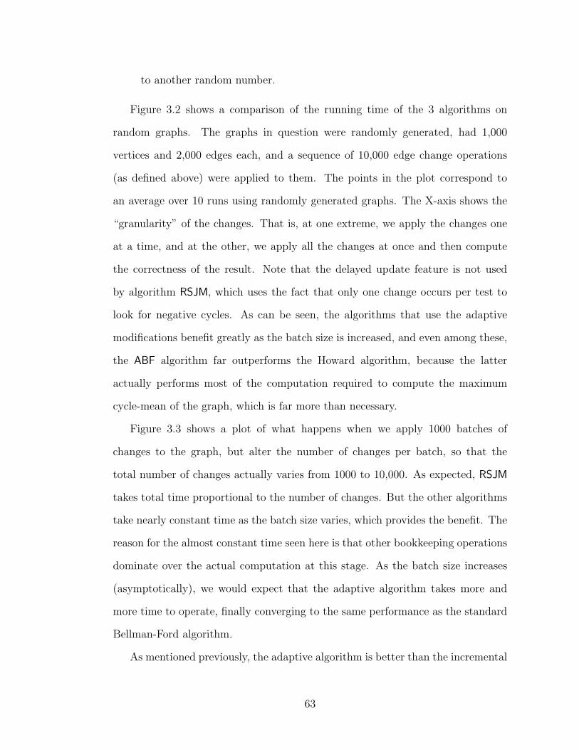
to another random number.
Figure 3.2 shows a comparison of the running time of the 3 algorithms on
random graphs. The graphs in question were randomly generated, had 1,000
vertices and 2,000 edges each, and a sequence of 10,000 edge change operations
(as defined above) were applied to them. The points in the plot correspond to
an average over 10 runs using randomly generated graphs. The X-axis shows the
“granularity” of the changes. That is, at one extreme, we apply the changes one
at a time, and at the other, we apply all the changes at once and then compute
the correctness of the result. Note that the delayed update feature is not used
by algorithm RSJM, which uses the fact that only one change occurs per test to
look for negative cycles. As can be seen, the algorithms that use the adaptive
modifications benefit greatly as the batch size is increased, and even among these,
the ABF algorithm far outperforms the Howard algorithm, because the latter
actually performs most of the computation required to compute the maximum
cycle-mean of the graph, which is far more than necessary.
Figure 3.3 shows a plot of what happens when we apply 1000 batches of
changes to the graph, but alter the number of changes per batch, so that the
total number of changes actually varies from 1000 to 10,000. As expected, RSJM
takes total time proportional to the number of changes. But the other algorithms
take nearly constant time as the batch size varies, which provides the benefit. The
reason for the almost constant time seen here is that other bookkeeping operations
dominate over the actual computation at this stage. As the batch size increases
(asymptotically), we would expect that the adaptive algorithm takes more and
more time to operate, finally converging to the same performance as the standard
Bellman-Ford algorithm.
As mentioned previously, the adaptive algorithm is better than the incremental
63
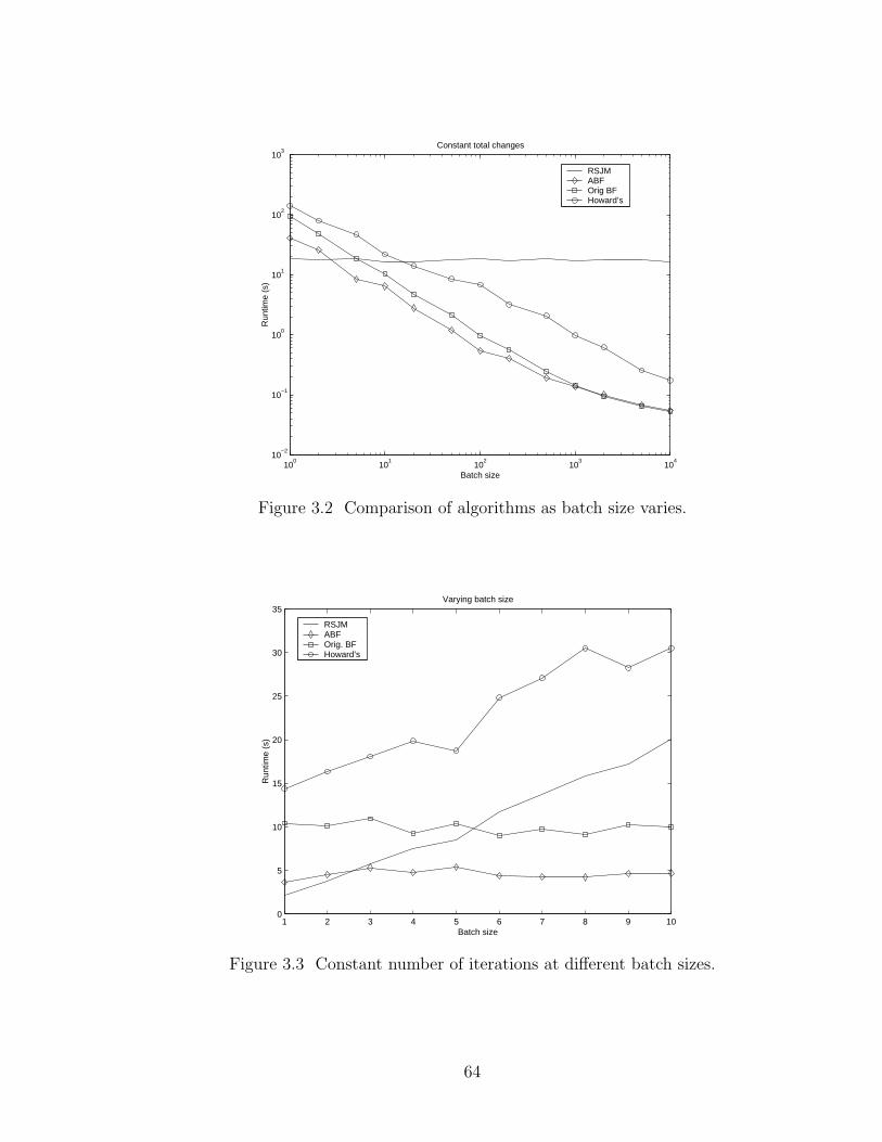
100
101
102
103
104
10−2
10−1
100
101
102
103
Constant total changes
Batch size
Run
time
(s)
RSJM ABF Orig BF Howard’s
Figure 3.2 Comparison of algorithms as batch size varies.
1 2 3 4 5 6 7 8 9 100
5
10
15
20
25
30
35
Batch size
Run
time
(s)
Varying batch size
RSJM ABF Orig. BFHoward’s
Figure 3.3 Constant number of iterations at different batch sizes.
64
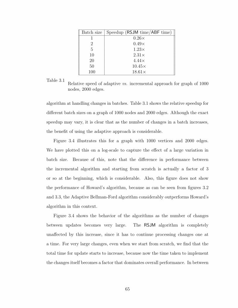
Batch size Speedup (RSJM time/ABF time)1 0.26×2 0.49×5 1.23×10 2.31×20 4.44×50 10.45×100 18.61×
Table 3.1Relative speed of adaptive vs. incremental approach for graph of 1000nodes, 2000 edges.
algorithm at handling changes in batches. Table 3.1 shows the relative speedup for
different batch sizes on a graph of 1000 nodes and 2000 edges. Although the exact
speedup may vary, it is clear that as the number of changes in a batch increases,
the benefit of using the adaptive approach is considerable.
Figure 3.4 illustrates this for a graph with 1000 vertices and 2000 edges.
We have plotted this on a log-scale to capture the effect of a large variation in
batch size. Because of this, note that the difference in performance between
the incremental algorithm and starting from scratch is actually a factor of 3
or so at the beginning, which is considerable. Also, this figure does not show
the performance of Howard’s algorithm, because as can be seen from figures 3.2
and 3.3, the Adaptive Bellman-Ford algorithm considerably outperforms Howard’s
algorithm in this context.
Figure 3.4 shows the behavior of the algorithms as the number of changes
between updates becomes very large. The RSJM algorithm is completely
unaffected by this increase, since it has to continue processing changes one at
a time. For very large changes, even when we start from scratch, we find that the
total time for update starts to increase, because now the time taken to implement
the changes itself becomes a factor that dominates overall performance. In between
65
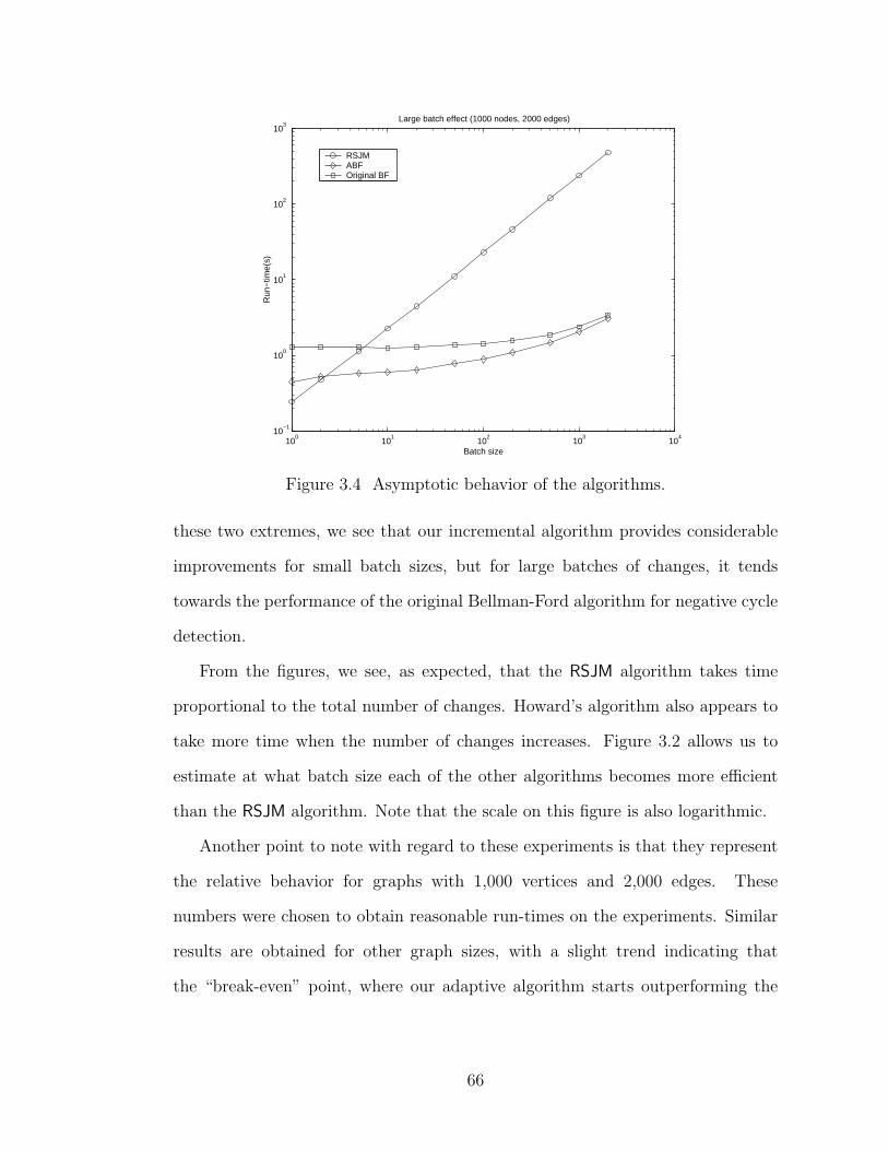
100
101
102
103
104
10−1
100
101
102
103
Large batch effect (1000 nodes, 2000 edges)
Batch size
Run
−tim
e(s)
RSJM ABF Original BF
Figure 3.4 Asymptotic behavior of the algorithms.
these two extremes, we see that our incremental algorithm provides considerable
improvements for small batch sizes, but for large batches of changes, it tends
towards the performance of the original Bellman-Ford algorithm for negative cycle
detection.
From the figures, we see, as expected, that the RSJM algorithm takes time
proportional to the total number of changes. Howard’s algorithm also appears to
take more time when the number of changes increases. Figure 3.2 allows us to
estimate at what batch size each of the other algorithms becomes more efficient
than the RSJM algorithm. Note that the scale on this figure is also logarithmic.
Another point to note with regard to these experiments is that they represent
the relative behavior for graphs with 1,000 vertices and 2,000 edges. These
numbers were chosen to obtain reasonable run-times on the experiments. Similar
results are obtained for other graph sizes, with a slight trend indicating that
the “break-even” point, where our adaptive algorithm starts outperforming the
66
incremental approach, shifts to lower batch-sizes for larger graphs.
3.6 Application: Maximum Cycle Mean computation
As an application of the adaptive negative cycle detection, we consider the
computation of the Maximum Cycle Mean (MCM) of a weighted digraph. This
quantity is defined as
maxc∈C
∑e∈c t(e)∑e∈c d(e)
,
where t(e) and d(e) are costs associated with the edges in the graph, and C is the
set of all directed cycles in the graph G.
For the digraph corresponding to the constraint graph of a dataflow system,
the maximum cycle mean is a useful performance metric. It is defined as the
maximum over all directed cycles in the graph, of the sum of the arc weights
divided by the number of delay elements on the arcs. This metric plays an
important role in discrete systems and embedded systems [35, 60], since it
represents the greatest throughput that can be extracted from the system. Also,
as mentioned in [60], there are situations where it may be desirable to recompute
this measure several times on closely related graphs, for example for the purpose
of design space exploration. As specific examples, [70] proposes an algorithm
for dataflow graph partitioning where the repeated computation of the MCM
plays a key role, and [11] discusses the utility of frequent MCM computation
to synchronization optimization in embedded multiprocessors. Therefore, efficient
algorithms for this problem can make it reasonable to consider using such solutions
instead of the simpler heuristics that are otherwise necessary. Although several
results such as [27, 51] provide polynomial time algorithms for the problem of
MCM computation, the first extensive study of algorithmic alternatives for it has
67
been undertaken by Dasdan et al. [35]. They concluded that the best existing
algorithm in practice for this problem appears to be Howard’s algorithm, which,
unfortunately, does not have a known polynomial bound on its running time.
To model this application, the edge weights on our graph are obtained from
the equation
weight(u → v) = delay(e)× P − exec time(u),
where weight(e) refers to the weight of the edge e : u → v, delay(e) refers to the
number of delay elements (flip-flops) on the edge, exec time(u) is the propagation
delay of the circuit element that is the source of the vertex, and P is the desired
clock period that we are testing the system for. In other words, if the graph with
weights as mentioned above does not have negative cycles, then P is a feasible
clock for the system. We can then perform a binary search in order to compute
P to any precision we require. This algorithm is attributed to Lawler [64]. Our
contribution here is to apply the adaptive negative-cycle detection techniques to
this algorithm and analyze the improved algorithm that is obtained as a result.
3.6.1 Experimental setup
For an experimental study, we build on the work by Dasdan and Gupta [35],
where the authors have conducted an extensive study of algorithms for this
problem. They conclude that Howard’s algorithm [31] appears to be the fastest
experimentally, even though no theoretical time bounds indicate this. As will
be seen, our algorithm performs almost as well as Howard’s algorithm on several
useful sized graphs, and especially on the circuits of the ISCAS 89/93 benchmarks,
where our algorithm typically performs better.
For comparison purposes, we implemented our algorithm in the C programming
68
language, and compared it against the implementation provided by the authors
of [31]. Although the authors do not claim their implementation is the fastest
possible, it appears to be a very efficient implementation, and we could not find
any obvious ways of improving it. The implementation we used incorporates
the improvements proposed by Dasdan et al. [35]. The experiments were run
on a Sun Ultra SPARC-10 (333MHz processor, 128MB memory). This machine
would classify as a medium-range workstation at the time the experiments were
conducted.
Based on the known complexity of the Bellman-Ford algorithm, the best
performance bound that can be placed on the algorithm as it stands is
O(|V ||E| log T ) where T is the maximum value of P that we examine in the search
procedure, and |V | and |E| are respectively the size of the input graph in number
of vertices and edges. However, our experiments show that it performs significantly
faster than would be expected by this bound.
One point to note is that since we are doing a binary search on T , we are forced
to set a limit on the precision to which we compute our answer. This precision
in turn depends on the maximum value of the edge-weights, as well as the actual
precision desired in the application itself. Since these depend on the application,
we have had to choose values for these. We have used a random graph generator
that generates integer weights for the edges in the range [0-10,000]. Previous
studies of algorithms for the MCM, such as used in [51, 86, 81], consider integer
weights for execution times, and correspondingly, the iteration period bound would
also be an integer. This is true, for example, if the operations are implemented in
software and the execution time corresponds to the number of clock cycles used
for computation. However, since the maximum cycle mean is a ratio, it is not
restricted to integer values. We have therefore conservatively chosen a precision
69
of 0.001 for the binary search (that is, 10−7 times the maximum edge-weight).
Increasing the precision by a factor of 2 requires one more run of the negative-
cycle detection algorithm, which would imply a proportionate increase in the total
time taken for computation of the MCM.
With regard to the ISCAS benchmarks [15], note that there is a slight
ambiguity in translating the net-lists into graphs. This arises because a D-type flip-
flop can either be treated as a single edge with a delay, with the fanout proceeding
from the sink of this edge, or as k separate edges with unit delay emanating from
the source vertex. In the former treatment, it makes more sense to talk about the
|D|/|V | ratio (|D| being the number of D flip-flops), as opposed to the |D|/|E|ratio that we use in the experiments with random graphs. However, the difference
between the two treatments is not significant and can be safely ignored.
We also conducted experiments where we vary the number of edges with delays
on them. For this, we need to exercise care, since we may introduce cycles without
delays on them, which are fundamentally infeasible and do not have a maximum
cycle-mean. To avoid this, we follow the policy of treating edges with delays as
“back-edges” in an otherwise acyclic graph [36]. This view is inspired by the
structure of circuits, where a delay element usually figures in the feedback portion
of the system. Unfortunately, one effect of this is that when we have a low number
of delay edges, the resulting graph tends to have an asymmetric structure: it is
almost acyclic with only a few edges in the reverse “direction”. It is not clear
how to get around this problem in a fashion that does not destroy the symmetry
of the graph, since this requires solving the feedback arc set problem, which is
NP-hard [47].
One effect of this is in the way it impacts the performance of the Bellman-
Ford algorithm. When the number of edges with delays is small, there are several
70

negative weight edges, which means that the standard Bellman-Ford algorithm
spends large amounts of time trying to compute shortest paths initially. The
incremental approach, however, is able to avoid this excess computation for large
values of T , which results in its performance being considerably faster when the
number of delays is small.
Intuitively, therefore, for the above situation, we would expect our algorithm
to perform better. This is because, for the MCM problem, a change in the value
of P for which we are testing the system will cause changes in the weights of
those edges which have delays on them. If these are fewer, then we would expect
that fewer operations would be required overall when we retain information across
iterations. This is borne out by the experiments as discussed in the next section.
Our experiments focus more on the kinds of graphs that are similar to the
graphs found in common digital signal processing and logic circuits. By this we
mean graphs for which the average out-degree of a vertex (number of edges divided
by number of vertices), and the relative number of edges with delays on them are
similar to those found in real circuits. We have used the ISCAS benchmarks
as a good representative sample of real circuits, and we can see that they show
remarkable similarity in the parameters we have described: the average out-degree
of a vertex is a little less than 2, while an average of about 1/10th or fewer edges
have delays on them. This is in accordance with the sparse structure of the graphs
that was discussed in section 3.5, which is a result of the nature of the components
comprising the overall circuit.
3.6.2 Experimental results
We now present the results of the experiments on random graphs with different
parameters of the graph being varied.
71
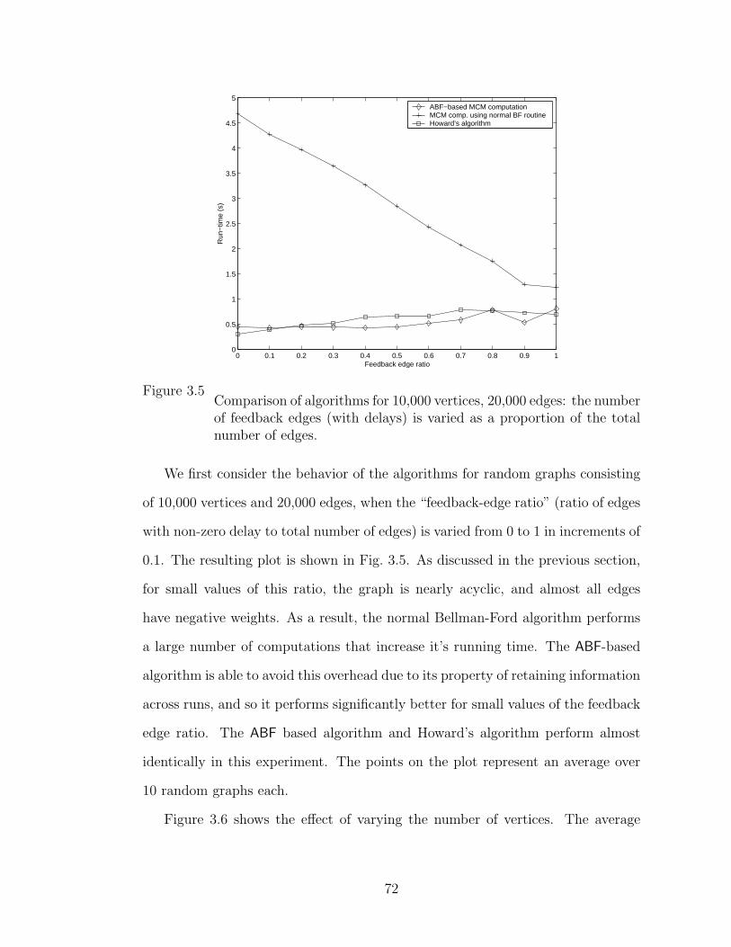
0 0.1 0.2 0.3 0.4 0.5 0.6 0.7 0.8 0.9 10
0.5
1
1.5
2
2.5
3
3.5
4
4.5
5
Feedback edge ratio
Run
−tim
e (s
)
ABF−based MCM computation MCM comp. using normal BF routineHoward’s algorithm
Figure 3.5Comparison of algorithms for 10,000 vertices, 20,000 edges: the numberof feedback edges (with delays) is varied as a proportion of the totalnumber of edges.
We first consider the behavior of the algorithms for random graphs consisting
of 10,000 vertices and 20,000 edges, when the “feedback-edge ratio” (ratio of edges
with non-zero delay to total number of edges) is varied from 0 to 1 in increments of
0.1. The resulting plot is shown in Fig. 3.5. As discussed in the previous section,
for small values of this ratio, the graph is nearly acyclic, and almost all edges
have negative weights. As a result, the normal Bellman-Ford algorithm performs
a large number of computations that increase it’s running time. The ABF-based
algorithm is able to avoid this overhead due to its property of retaining information
across runs, and so it performs significantly better for small values of the feedback
edge ratio. The ABF based algorithm and Howard’s algorithm perform almost
identically in this experiment. The points on the plot represent an average over
10 random graphs each.
Figure 3.6 shows the effect of varying the number of vertices. The average
72
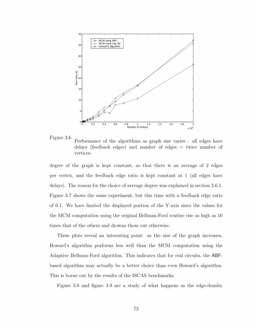
0 0.2 0.4 0.6 0.8 1 1.2 1.4 1.6 1.8 2
x 105
0
5
10
15
20
25
30
35
40
Number of vertices
Run
−tim
e (s
)
MCM using ABF MCM using orig. BFHoward’s algorithm
Figure 3.6Performance of the algorithms as graph size varies : all edges havedelays (feedback edges) and number of edges = twice number ofvertices.
degree of the graph is kept constant, so that there is an average of 2 edges
per vertex, and the feedback edge ratio is kept constant at 1 (all edges have
delays). The reason for the choice of average degree was explained in section 3.6.1.
Figure 3.7 shows the same experiment, but this time with a feedback edge ratio
of 0.1. We have limited the displayed portion of the Y-axis since the values for
the MCM computation using the original Bellman-Ford routine rise as high as 10
times that of the others and drowns them out otherwise.
These plots reveal an interesting point: as the size of the graph increases,
Howard’s algorithm performs less well than the MCM computation using the
Adaptive Bellman-Ford algorithm. This indicates that for real circuits, the ABF-
based algorithm may actually be a better choice than even Howard’s algorithm.
This is borne out by the results of the ISCAS benchmarks.
Figure 3.8 and figure 3.9 are a study of what happens as the edge-density
73
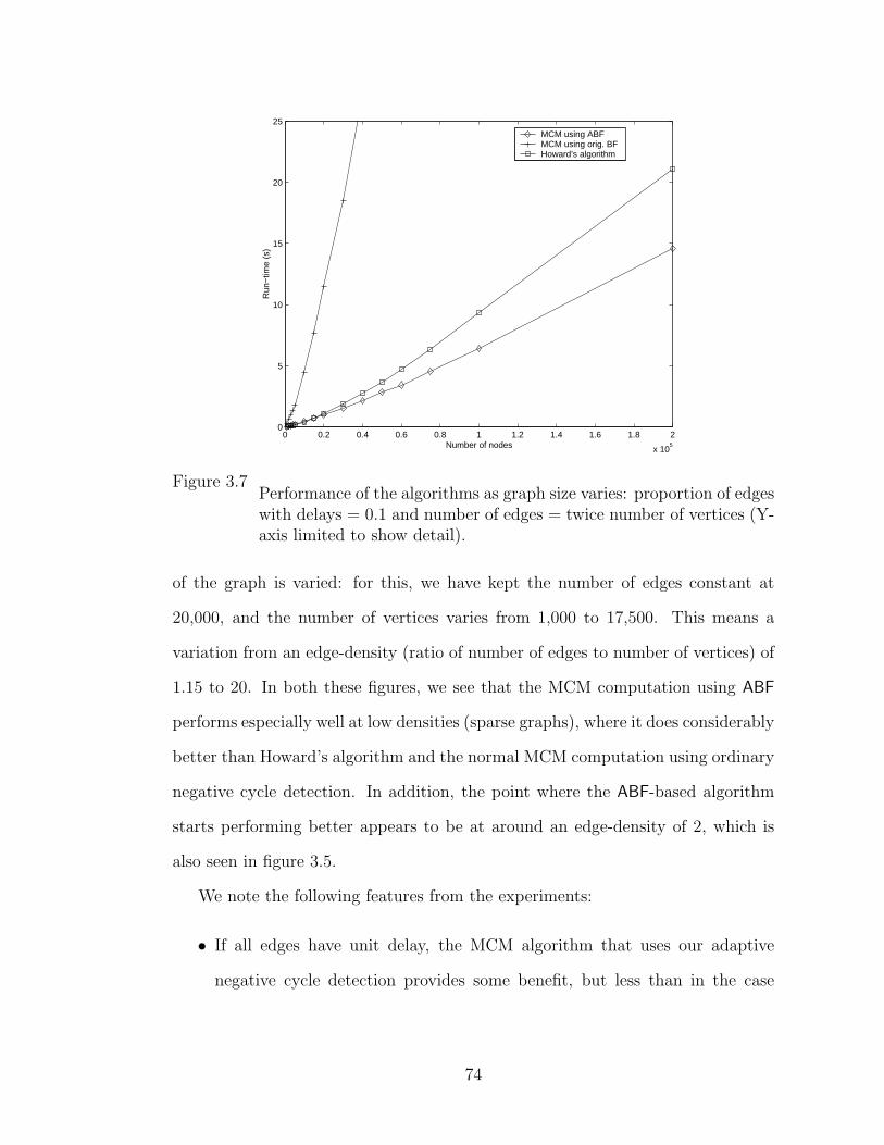
0 0.2 0.4 0.6 0.8 1 1.2 1.4 1.6 1.8 2
x 105
0
5
10
15
20
25
Number of nodes
Run
−tim
e (s
)
MCM using ABF MCM using orig. BFHoward’s algorithm
Figure 3.7Performance of the algorithms as graph size varies: proportion of edgeswith delays = 0.1 and number of edges = twice number of vertices (Y-axis limited to show detail).
of the graph is varied: for this, we have kept the number of edges constant at
20,000, and the number of vertices varies from 1,000 to 17,500. This means a
variation from an edge-density (ratio of number of edges to number of vertices) of
1.15 to 20. In both these figures, we see that the MCM computation using ABF
performs especially well at low densities (sparse graphs), where it does considerably
better than Howard’s algorithm and the normal MCM computation using ordinary
negative cycle detection. In addition, the point where the ABF-based algorithm
starts performing better appears to be at around an edge-density of 2, which is
also seen in figure 3.5.
We note the following features from the experiments:
• If all edges have unit delay, the MCM algorithm that uses our adaptive
negative cycle detection provides some benefit, but less than in the case
74
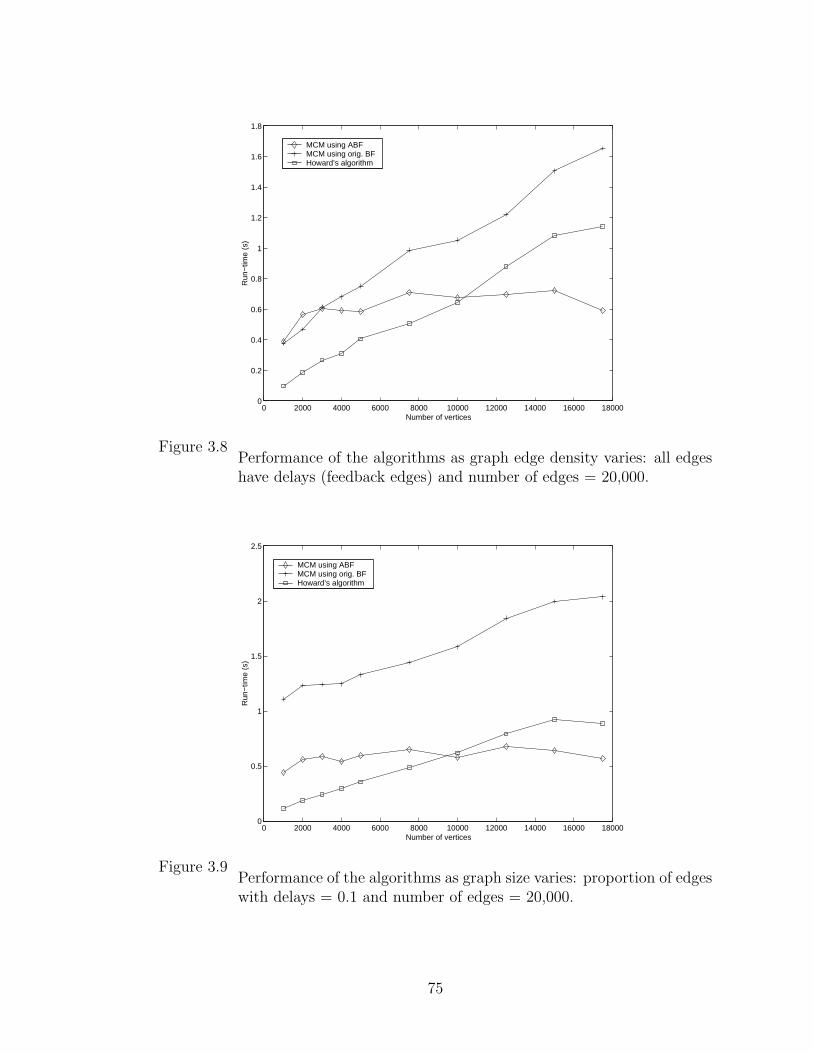
0 2000 4000 6000 8000 10000 12000 14000 16000 180000
0.2
0.4
0.6
0.8
1
1.2
1.4
1.6
1.8
Number of vertices
Run
−tim
e (s
)
MCM using ABF MCM using orig. BFHoward’s algorithm
Figure 3.8Performance of the algorithms as graph edge density varies: all edgeshave delays (feedback edges) and number of edges = 20,000.
0 2000 4000 6000 8000 10000 12000 14000 16000 180000
0.5
1
1.5
2
2.5
Number of vertices
Run
−tim
e (s
)
MCM using ABF MCM using orig. BFHoward’s algorithm
Figure 3.9Performance of the algorithms as graph size varies: proportion of edgeswith delays = 0.1 and number of edges = 20,000.
75
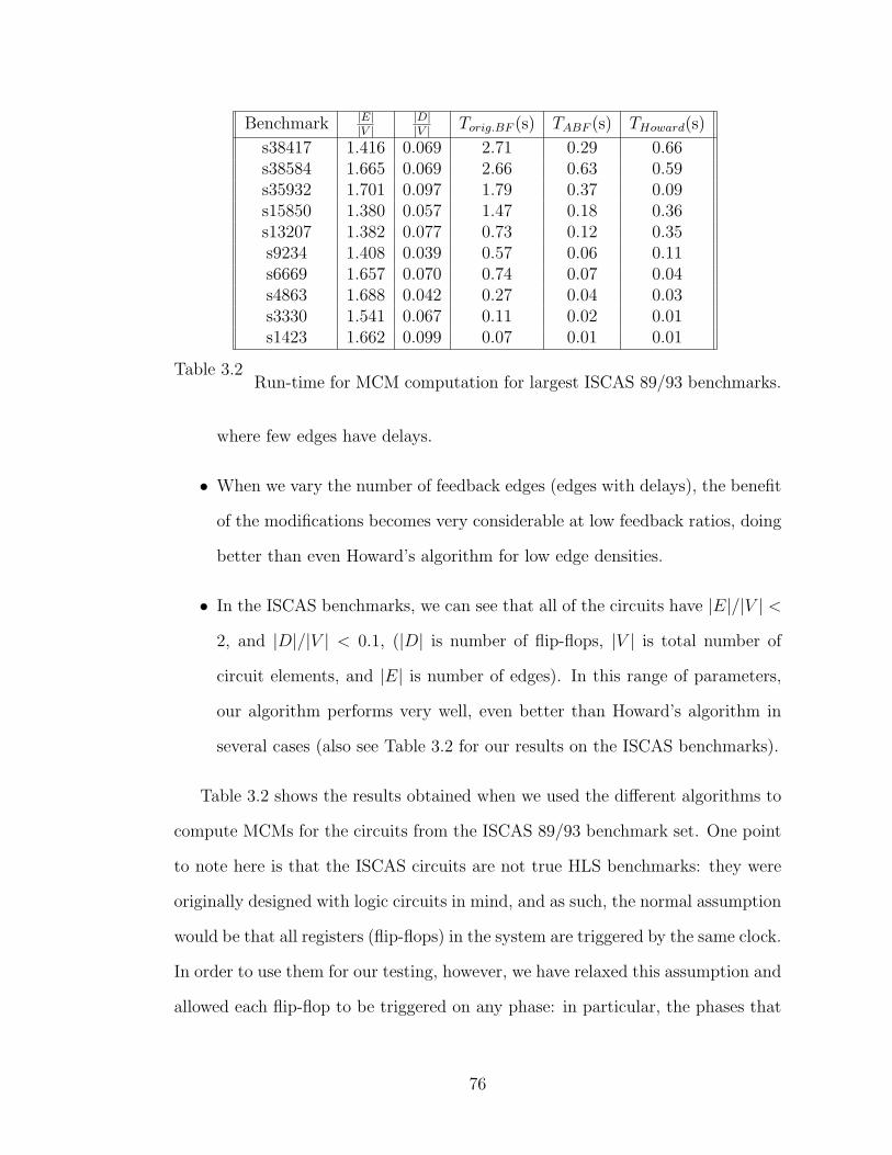
Benchmark |E||V |
|D||V | Torig.BF (s) TABF (s) THoward(s)
s38417 1.416 0.069 2.71 0.29 0.66s38584 1.665 0.069 2.66 0.63 0.59s35932 1.701 0.097 1.79 0.37 0.09s15850 1.380 0.057 1.47 0.18 0.36s13207 1.382 0.077 0.73 0.12 0.35s9234 1.408 0.039 0.57 0.06 0.11s6669 1.657 0.070 0.74 0.07 0.04s4863 1.688 0.042 0.27 0.04 0.03s3330 1.541 0.067 0.11 0.02 0.01s1423 1.662 0.099 0.07 0.01 0.01
Table 3.2Run-time for MCM computation for largest ISCAS 89/93 benchmarks.
where few edges have delays.
• When we vary the number of feedback edges (edges with delays), the benefit
of the modifications becomes very considerable at low feedback ratios, doing
better than even Howard’s algorithm for low edge densities.
• In the ISCAS benchmarks, we can see that all of the circuits have |E|/|V | <2, and |D|/|V | < 0.1, (|D| is number of flip-flops, |V | is total number of
circuit elements, and |E| is number of edges). In this range of parameters,
our algorithm performs very well, even better than Howard’s algorithm in
several cases (also see Table 3.2 for our results on the ISCAS benchmarks).
Table 3.2 shows the results obtained when we used the different algorithms to
compute MCMs for the circuits from the ISCAS 89/93 benchmark set. One point
to note here is that the ISCAS circuits are not true HLS benchmarks: they were
originally designed with logic circuits in mind, and as such, the normal assumption
would be that all registers (flip-flops) in the system are triggered by the same clock.
In order to use them for our testing, however, we have relaxed this assumption and
allowed each flip-flop to be triggered on any phase: in particular, the phases that
76
are computed by the MCM computation algorithm are such that the overall system
speed is maximized. Such operation has been previously considered as a method
for increasing system speed and safety margins [42, 100], so these benchmarks are
quite useful for our purpose. These benchmark circuits are also very important in
the area of HLS, because real DSP circuits show similar structure (sparseness and
density of delay elements), and an important observation we can make from the
experiments is that the structure of the graph is very relevant to the performance
of the various algorithms in the MCM computation.
The first column in the table is just the name of the benchmark circuit. The
second and third columns show the average degree (ratio of edges to vertices) and
the average feedback measure (ratio of number of flip-flops to total vertices) in the
graph. This indicates the sparseness and amount of feedback in the graph. The
last 3 columns indicate the run-time in seconds of the MCM computation on a Sun
UltraSparc II 333Mhz processor system with 128MB RAM. Torig.BF refers to the
original algorithm without the adaptive negative cycle detection, TABF is the run-
time using the ABF algorithm, and THoward is the run-time of the implementation
of Howard’s algorithm from [31].
As can be seen in the table, Lawler’s algorithm does reasonably well at
computing the MCM. However, when we use the adaptive negative cycle detection
in place of the normal negative cycle detection technique, there is an increase
in speed by a factor of 5 to 10 in most cases. This increase in speed is in fact
sufficient to make Lawler’s algorithm with this implementation up to twice as fast
as Howard’s algorithm, which was otherwise considered the fastest algorithm in
practice for this problem.
77
3.7 Conclusions
The problem of negative cycle detection is considered in the context of HLS for
DSP systems. It was shown that important problems such as performance analysis
and design space exploration often result in the construction of “dynamic” graphs,
where it is necessary to repeatedly perform negative cycle detection on variants of
the original graph.
We have introduced an adaptive approach (the ABF algorithm) to negative
cycle detection in dynamically changing graphs. Specifically, we have developed
an enhancement to Tarjan’s algorithm for detecting negative cycles in static
graphs. This enhancement yields a powerful algorithm for dynamic graphs
that outperforms previously available methods for addressing the scenario where
multiple changes are made to the graph between updates. Our technique explicitly
addresses the common, practical scenario in which negative cycle detection must
be periodically performed after intervals in which a small number of changes are
made to the graph. We have shown by experiments that for reasonable sized graphs
(10,000 vertices and 20,000 edges) our algorithm outperforms the incremental
algorithm (one change processed at a time) described in [94] even for changes
made in groups of as little as 4-5 at a time.
As our original interest in the negative cycle detection problem arose from
its application to problems in HLS, we have implemented some schemes that
make use of the adaptive approach to solve those problems. We have shown
how our adaptive approach to negative cycle detection can be exploited to
compute the maximum cycle mean of a weighted digraph, which is a relevant
metric for determining the throughput of DSP system implementations. We
have compared our ABF technique, and ABF-based MCM computation technique
78
against the best known related work in the literature, and have observed favorable
performance. Specifically, the new technique provides better performance than
Howard’s algorithm for sparse graphs with relatively few edges that have delays.
Since computing power is cheaply available now, it is increasingly worthwhile
to employ extensive search techniques for solving NP-hard analysis and design
problems such as scheduling. The availability of an efficient adaptive negative cycle
detection algorithm can make this process much more efficient in many application
contexts. Some of the search techniques discussed in chapter 5 show the advantages
of using the adaptive negative cycle detection for this purpose.
79
Chapter 4
Hierarchical timing representation
4.1 Introduction
This chapter deals with the problem of representing the timing information
associated with the operating elements in a system for HLS. For combinational
circuits used in ordinary circuit design, the longest execution path (critical path)
is clearly defined, and can be used to represent the timing of the whole circuit for
the purpose of performance analysis. In sequential circuits, the presence of delay
elements (registers) on edges introduces a time shift that is related to the clock
period used on the system. This means that the longest combinational path no
longer represents the timing of the circuit.
We introduce the concept of Timing Pairs to model delay elements in
sequential and multirate circuits, and show how this allows us to derive hierarchical
timing information for complex circuits. The resulting compact representation of
the timing information can be used to streamline system performance analysis.
In addition, several analytical results that previously applied only to single rate
systems can now be extended to multirate systems.
We begin with some reasons why a hierarchical timing representation is useful
80
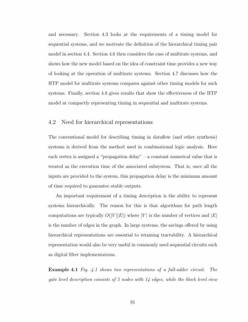
and necessary. Section 4.3 looks at the requirements of a timing model for
sequential systems, and we motivate the definition of the hierarchical timing pair
model in section 4.4. Section 4.6 then considers the case of multirate systems, and
shows how the new model based on the idea of constraint time provides a new way
of looking at the operation of multirate systems. Section 4.7 discusses how the
HTP model for multirate systems compares against other timing models for such
systems. Finally, section 4.8 gives results that show the effectiveness of the HTP
model at compactly representing timing in sequential and multirate systems.
4.2 Need for hierarchical representations
The conventional model for describing timing in dataflow (and other synthesis)
systems is derived from the method used in combinational logic analysis. Here
each vertex is assigned a “propagation delay” – a constant numerical value that is
treated as the execution time of the associated subsystem. That is, once all the
inputs are provided to the system, this propagation delay is the minimum amount
of time required to guarantee stable outputs.
An important requirement of a timing description is the ability to represent
systems hierarchically. The reason for this is that algorithms for path length
computations are typically O(|V ||E|) where |V | is the number of vertices and |E|is the number of edges in the graph. In large systems, the savings offered by using
hierarchical representations are essential to retaining tractability. A hierarchical
representation would also be very useful in commonly used sequential circuits such
as digital filter implementations.
Example 4.1 Fig. 4.1 shows two representations of a full-adder circuit. The
gate level description consists of 5 nodes with 14 edges, while the block level view
81
(a)
(b)
Figure 4.1 (a) Full adder circuit. (b) Hierarchical block view.
replaces this by a single node with 3 inputs and 2 outputs. If this circuit was used
as a sub-circuit in a larger design containing 10 full-adder elements, the gate level
description would have a size of 50 nodes and on the order of 100 or so edges,
while the block level description would consist of 10 nodes with about 20 edges.
A major disadvantage of the conventional timing model is that it does not allow
a hierarchical description of iterative systems (containing delay elements). These
delay elements correspond to registers in a hardware implementation, but are more
flexible in that they do not impose the restriction that all the delay elements are
activated at the same instant of time [88, 86, 36]. To be more accurate, the delay
elements mark the boundary points where the computation on either side of the
delay element uses data values corresponding to a different time index. This is
primarily important in filters and other structures that operate on semi-infinite
data streams. The rephasing optimization in [88] provides a good example of how
the flexibility in assigning clock phases can be used to improve the performance
of a design.
In the case of sequential circuitry, it is possible to allow variable phase clocking
for the registers in the circuit. In sequential logic synthesis, variable phase
clocking has been considered in such forms as clock skew optimization [42, 100]
82

and shimming delays [61]. This has been recognized as a very useful tool, though
it is difficult to implement in practice. Skew optimization and variable phase
clocking have also been found useful in attacking the problem of retiming sequential
circuitry for minimum period [97, 28] and area [72].
In multirate SDF graphs, the standard interpretation of execution time is as
follows [66]: each vertex is assumed to be enabled when sufficient dataflow tokens
have enqueued on its inputs. Once it is enabled in this fashion, it can fire at any
time, consuming a number of tokens from each input edge equal to the consumption
parameter on that edge, and producing a number of tokens on each output edge
equal to the production parameter on that edge. The execution time of the vertex
is the time between the (instantaneous) consumption and production events.
This model has been used in the context of SDF to derive several useful results
regarding consistency, liveness and throughput of graphs modeling DSP systems.
However, the treatment is quite different from that for homogeneous graphs, and
many analytical results for homogeneous systems cannot be extended to multirate
systems. Several attempts have been made to derive results for the performance
bounds [101] and retimability [118, 80] of multirate SDF graphs, but the standard
semantics of execution have not so far yielded closed-form expressions for such
metrics. Most of the work has required converting the multirate graph into the
equivalent homogeneous graph, and since this conversion can result in exponential
increase in the size of the resulting graph, the algorithms may not be very efficient.
In addition, the economy of expression provided by the multirate representation
is lost.
To the best of our knowledge, there does not appear to be any other timing
model that addresses the hierarchical timing issues for dataflow based DSP system
design. Conventional models cannot easily be used to represent systems that are
83
either hierarchical or contain multirate elements. Models such as the processor
timing data used in [111] capture the effects of real system parameters and latency
for single rate systems, but they do not provide ways to take advantage of skewed
clock phases or multirate graphs directly. Multirate systems are usually handled by
expanding to the equivalent homogeneous graph (which can lead to an exponential
increase in the graph size), while hierarchical systems need to be completely
flattened and expanded in the context of the overall graph. The relationship
of our model to other models is examined in more detail in sec. 4.7.
We propose a different timing model that overcomes these difficulties for
dedicated hardware implementations of the dataflow graph. By introducing a
slightly more complex data structure that allows for multiple input-output paths
with differing numbers of delay elements, we are able to provide a single timing
model that can describe both purely combinational and iterative systems. For
purely combinational systems, the model reduces to the existing combinational
logic timing model. For multirate systems, the new model allows a treatment
very similar to that for normal homogeneous systems, while still allowing most
important features of the multirate execution to be represented. The model
also allows analytical results for homogeneous systems to be applied to multirate
systems. As an example, we derive an expression for the iteration period bound
of a multirate graph.
We have used our hierarchical timing model to compute timing parameters
of the ISCAS benchmarks, which are homogeneous systems. We have also used
the model to compute timing parameters of a number of multirate graphs used
in signal processing applications. The results show that the new model can
result in compact representations of fairly large systems that can then be used
as hierarchical subsystems of larger graphs. These results show a large savings in
84
complexity by using the new approach.
Portions of these results were published in [22] and [21], for the timing pair
model and its extension to multirate systems, respectively.
4.3 Requirements of a Timing Model for Hierarchical Systems
In deriving the model presented in the next section, we make certain assumptions
about the system being represented, and also about the goals of a timing
representation. These are clarified in this section.
4.3.1 SISO system
We focus on Single-Input Single-Output (SISO) systems. For general Multiple-
Input Multiple-Output (MIMO) systems, each input/output pair can have
different path lengths resulting in different values for the longest combinational
path between them. However, we commonly assume a single value for the delay,
which is equivalent to assuming a single dummy input vertex and a dummy output
vertex, where all the inputs and outputs synchronize. More accurate models
actually do provide “bit-level timing” where they provide further information that
specifies the timing on input-output pairs, but these are rarely used.
Example 4.2 Fig. 4.2 shows the detailed timing of a 2-input 2-bit adder circuit
(based on examples from [63]). Part (a) shows the actual delay network
corresponding to the AND, OR and XOR gates that make up the circuit. Part (b) shows
the equivalent input-output network, where each input has a direct connection to
each output with the corresponding longest path as the delay amount. Here we can
see that most of the paths are actually only 2ns, but the longest I/O path is 4 ns.
For truly accurate timing analysis, we should store all the information in (b) in a
85
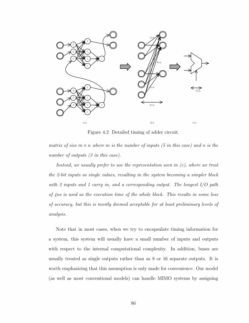
0
0
0
1
1
1
1
2
0
0
0
1
1
1
1
2
4ns
2ns
4ns
2ns
(a) (b) (c)
4ns
Figure 4.2 Detailed timing of adder circuit.
matrix of size m×n where m is the number of inputs (5 in this case) and n is the
number of outputs (3 in this case).
Instead, we usually prefer to use the representation seen in (c), where we treat
the 2-bit inputs as single values, resulting in the system becoming a simpler block
with 2 inputs and 1 carry in, and a corresponding output. The longest I/O path
of 4ns is used as the execution time of the whole block. This results in some loss
of accuracy, but this is mostly deemed acceptable for at least preliminary levels of
analysis.
Note that in most cases, when we try to encapsulate timing information for
a system, this system will usually have a small number of inputs and outputs
with respect to the internal computational complexity. In addition, buses are
usually treated as single outputs rather than as 8 or 16 separate outputs. It is
worth emphasizing that this assumption is only made for convenience. Our model
(as well as most conventional models) can handle MIMO systems by assigning
86
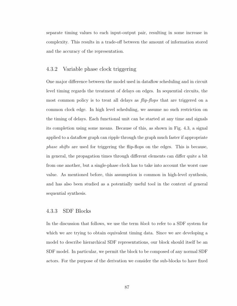
separate timing values to each input-output pair, resulting in some increase in
complexity. This results in a trade-off between the amount of information stored
and the accuracy of the representation.
4.3.2 Variable phase clock triggering
One major difference between the model used in dataflow scheduling and in circuit
level timing regards the treatment of delays on edges. In sequential circuits, the
most common policy is to treat all delays as flip-flops that are triggered on a
common clock edge. In high level scheduling, we assume no such restriction on
the timing of delays. Each functional unit can be started at any time and signals
its completion using some means. Because of this, as shown in Fig. 4.3, a signal
applied to a dataflow graph can ripple through the graph much faster if appropriate
phase shifts are used for triggering the flip-flops on the edges. This is because,
in general, the propagation times through different elements can differ quite a bit
from one another, but a single-phase clock has to take into account the worst case
value. As mentioned before, this assumption is common in high-level synthesis,
and has also been studied as a potentially useful tool in the context of general
sequential synthesis.
4.3.3 SDF Blocks
In the discussion that follows, we use the term block to refer to a SDF system for
which we are trying to obtain equivalent timing data. Since we are developing a
model to describe hierarchical SDF representations, our block should itself be an
SDF model. In particular, we permit the block to be composed of any normal SDF
actors. For the purpose of the derivation we consider the sub-blocks to have fixed
87
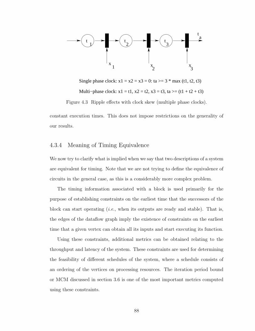
Single phase clock: x1 = x2 = x3 = 0: ta >= 3 * max (t1, t2, t3)
at
t1
t2
t3
1 2 3x x x
Multi−phase clock: x1 = t1, x2 = t2, x3 = t3, ta >= (t1 + t2 + t3)
Figure 4.3 Ripple effects with clock skew (multiple phase clocks).
constant execution times. This does not impose restrictions on the generality of
our results.
4.3.4 Meaning of Timing Equivalence
We now try to clarify what is implied when we say that two descriptions of a system
are equivalent for timing. Note that we are not trying to define the equivalence of
circuits in the general case, as this is a considerably more complex problem.
The timing information associated with a block is used primarily for the
purpose of establishing constraints on the earliest time that the successors of the
block can start operating (i.e., when its outputs are ready and stable). That is,
the edges of the dataflow graph imply the existence of constraints on the earliest
time that a given vertex can obtain all its inputs and start executing its function.
Using these constraints, additional metrics can be obtained relating to the
throughput and latency of the system. These constraints are used for determining
the feasibility of different schedules of the system, where a schedule consists of
an ordering of the vertices on processing resources. The iteration period bound
or MCM discussed in section 3.6 is one of the most important metrics computed
using these constraints.
88
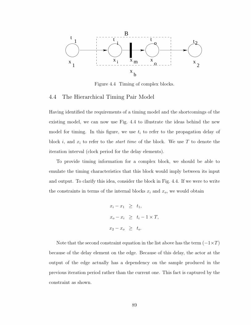
i
B
x1
x xo
xb
x2
t1 t
o t2
x m
it
Figure 4.4 Timing of complex blocks.
4.4 The Hierarchical Timing Pair Model
Having identified the requirements of a timing model and the shortcomings of the
existing model, we can now use Fig. 4.4 to illustrate the ideas behind the new
model for timing. In this figure, we use ti to refer to the propagation delay of
block i, and xi to refer to the start time of the block. We use T to denote the
iteration interval (clock period for the delay elements).
To provide timing information for a complex block, we should be able to
emulate the timing characteristics that this block would imply between its input
and output. To clarify this idea, consider the block in Fig. 4.4. If we were to write
the constraints in terms of the internal blocks xi and xo, we would obtain
xi − x1 ≥ t1,
xo − xi ≥ ti − 1× T,
x2 − xo ≥ to.
Note that the second constraint equation in the list above has the term (−1×T )
because of the delay element on the edge. Because of this delay, the actor at the
output of the edge actually has a dependency on the sample produced in the
previous iteration period rather than the current one. This fact is captured by the
constraint as shown.
89

Now we would like to compute certain information such that if we were to
combine the complex block B under the single start time xb, we would still be able
to write down equations that can provide the same constraints to the environment
outside the block B. We see that this is achieved by the following constraints:
xb − x1 ≥ t1,
x2 − xb ≥ ti + to − 1× T.
In other words, if we assume that the execution time of the block B is given by
the expression ti + to − 1× T , we can formulate constraints that exactly simulate
the effect of the complex block B.
In general, consider a path from input vi = v1 to output vo = vk through
vertices {v1, . . . , vk} given by p : v1→v2→· · ·→vk, with edges ei : vi→vi+1. Let
ti be the execution time (propagation delay assuming it is a simple combinational
block) of vi, and let dj be the number of delays on edge ej. Now we can define the
constraint time of this path as
tc(p) =k∑
i=1
ti − T ×k−1∑
j=1
dj. (4.1)
We use the term “constraint time” to refer to this quantity because it is in
some sense very similar to the notion of the execution time of the entire path, but
at the same time is relevant only within the context of the constraint system it is
used to build. The term cp is used to refer to the sum∑k
i=1 ti, and mp refers to
the sum∑k−1
j=1 dj. The ordered pair (mp, cp) is referred to as a timing pair. The
terms mp and cp were chosen because they are commonly used in mathematical
literature to refer to the slope and intercept of a line, which is the role they play
here. That is, the constraint time of a path varies linearly as the iteration period
T associated with the system changes. The slope of the line is given by mp and cp
is the intercept corresponding to T = 0.
90
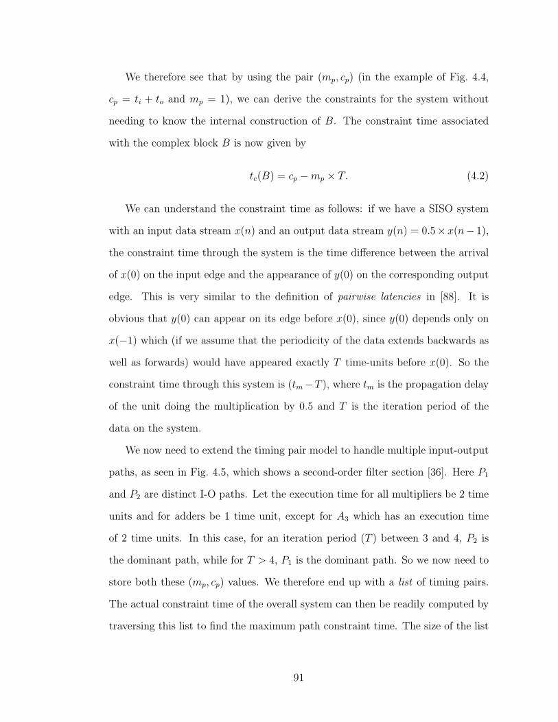
We therefore see that by using the pair (mp, cp) (in the example of Fig. 4.4,
cp = ti + to and mp = 1), we can derive the constraints for the system without
needing to know the internal construction of B. The constraint time associated
with the complex block B is now given by
tc(B) = cp −mp × T. (4.2)
We can understand the constraint time as follows: if we have a SISO system
with an input data stream x(n) and an output data stream y(n) = 0.5× x(n− 1),
the constraint time through the system is the time difference between the arrival
of x(0) on the input edge and the appearance of y(0) on the corresponding output
edge. This is very similar to the definition of pairwise latencies in [88]. It is
obvious that y(0) can appear on its edge before x(0), since y(0) depends only on
x(−1) which (if we assume that the periodicity of the data extends backwards as
well as forwards) would have appeared exactly T time-units before x(0). So the
constraint time through this system is (tm−T ), where tm is the propagation delay
of the unit doing the multiplication by 0.5 and T is the iteration period of the
data on the system.
We now need to extend the timing pair model to handle multiple input-output
paths, as seen in Fig. 4.5, which shows a second-order filter section [36]. Here P1
and P2 are distinct I-O paths. Let the execution time for all multipliers be 2 time
units and for adders be 1 time unit, except for A3 which has an execution time
of 2 time units. In this case, for an iteration period (T ) between 3 and 4, P2 is
the dominant path, while for T > 4, P1 is the dominant path. So we now need to
store both these (mp, cp) values. We therefore end up with a list of timing pairs.
The actual constraint time of the overall system can then be readily computed by
traversing this list to find the maximum path constraint time. The size of the list
91
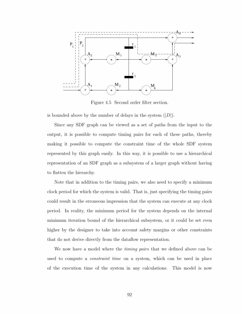
+
+
+
+
*
**
*
A
A
A
AM
MM
M
1
2 3
4
1
2
3
4
r
r2
1PP 21
Figure 4.5 Second order filter section.
is bounded above by the number of delays in the system (|D|).Since any SDF graph can be viewed as a set of paths from the input to the
output, it is possible to compute timing pairs for each of these paths, thereby
making it possible to compute the constraint time of the whole SDF system
represented by this graph easily. In this way, it is possible to use a hierarchical
representation of an SDF graph as a subsystem of a larger graph without having
to flatten the hierarchy.
Note that in addition to the timing pairs, we also need to specify a minimum
clock period for which the system is valid. That is, just specifying the timing pairs
could result in the erroneous impression that the system can execute at any clock
period. In reality, the minimum period for the system depends on the internal
minimum iteration bound of the hierarchical subsystem, or it could be set even
higher by the designer to take into account safety margins or other constraints
that do not derive directly from the dataflow representation.
We now have a model where the timing pairs that we defined above can be
used to compute a constraint time on a system, which can be used in place
of the execution time of the system in any calculations. This model is now
92
capable of handling both combinational and iterative systems, and can capture
the hierarchical nature of these systems easily. We therefore refer to it as the
Hierarchical Timing Pair (HTP) Model.
This definition of constraint time also results in a simple method for
determining the iteration period or maximum cycle mean of the graph. It is obvious
that the constraint time around a cycle must be negative to avoid unsatisfiable
dependencies. Also, note that for a fixed value of T , the constraint time of each
subsystem becomes a fixed number rather than a list of timing pairs. Because of
this, any algorithm that iterates over different values of T in order to determine
the best value that is feasible for the graph will only have to deal with the final
constraint time values and not the timing pair lists. As discussed in chapter 3,
Lawler’s method [64] provides an efficient way of doing this. It performs a sequence
of successive approximations to find a close approximation to the iteration period
T . This algorithm provides an effective way of computing the iteration period for
graphs described using the hierarchical model. It may be possible to find other
algorithms that can operate directly on the timing pair lists and compute a closed-
form analytical expression for the maximum cycle mean of the system. However,
since Lawler’s method is already known to be efficient in practice, this is not a
very urgent requirement.
4.5 Data Structure and Algorithms
We now present an efficient algorithm to compute the list of timing pairs associated
with a given dataflow graph. As seen in the previous section, it is possible to have
multiple input-output paths in the system, each with different numbers of delay
elements. When two paths differ in the number of delay elements, the actual
93
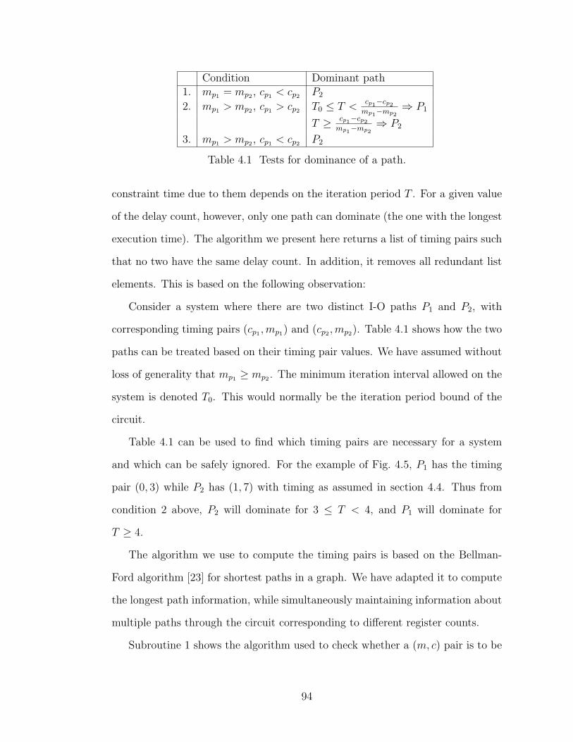
Condition Dominant path1. mp1 = mp2 , cp1 < cp2 P2
2. mp1 > mp2 , cp1 > cp2 T0 ≤ T <cp1−cp2
mp1−mp2⇒ P1
T ≥ cp1−cp2
mp1−mp2⇒ P2
3. mp1 > mp2 , cp1 < cp2 P2
Table 4.1 Tests for dominance of a path.
constraint time due to them depends on the iteration period T . For a given value
of the delay count, however, only one path can dominate (the one with the longest
execution time). The algorithm we present here returns a list of timing pairs such
that no two have the same delay count. In addition, it removes all redundant list
elements. This is based on the following observation:
Consider a system where there are two distinct I-O paths P1 and P2, with
corresponding timing pairs (cp1 ,mp1) and (cp2 ,mp2). Table 4.1 shows how the two
paths can be treated based on their timing pair values. We have assumed without
loss of generality that mp1 ≥ mp2 . The minimum iteration interval allowed on the
system is denoted T0. This would normally be the iteration period bound of the
circuit.
Table 4.1 can be used to find which timing pairs are necessary for a system
and which can be safely ignored. For the example of Fig. 4.5, P1 has the timing
pair (0, 3) while P2 has (1, 7) with timing as assumed in section 4.4. Thus from
condition 2 above, P2 will dominate for 3 ≤ T < 4, and P1 will dominate for
T ≥ 4.
The algorithm we use to compute the timing pairs is based on the Bellman-
Ford algorithm [23] for shortest paths in a graph. We have adapted it to compute
the longest path information, while simultaneously maintaining information about
multiple paths through the circuit corresponding to different register counts.
Subroutine 1 shows the algorithm used to check whether a (m, c) pair is to be
94
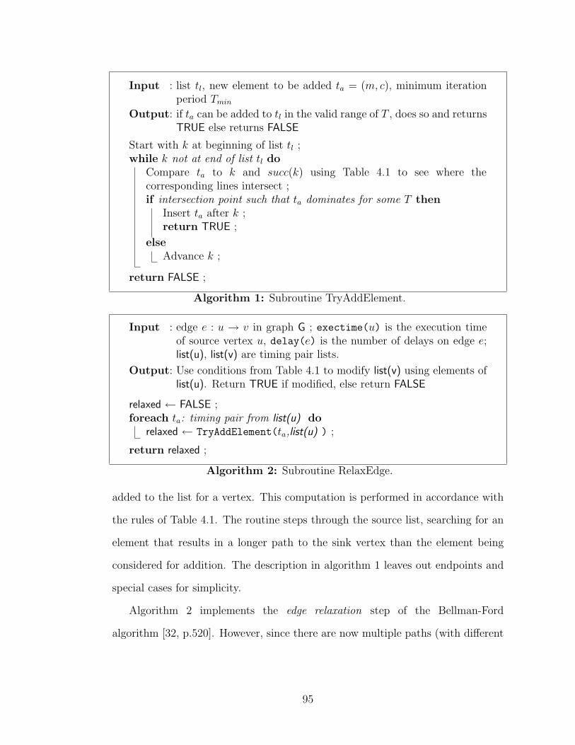
Input : list tl, new element to be added ta = (m, c), minimum iterationperiod Tmin
Output: if ta can be added to tl in the valid range of T , does so and returnsTRUE else returns FALSE
Start with k at beginning of list tl ;while k not at end of list tl do
Compare ta to k and succ(k) using Table 4.1 to see where thecorresponding lines intersect ;if intersection point such that ta dominates for some T then
Insert ta after k ;return TRUE ;
elseAdvance k ;
return FALSE ;
Algorithm 1: Subroutine TryAddElement.
Input : edge e : u → v in graph G ; exectime(u) is the execution timeof source vertex u, delay(e) is the number of delays on edge e;list(u), list(v) are timing pair lists.
Output: Use conditions from Table 4.1 to modify list(v) using elements oflist(u). Return TRUE if modified, else return FALSE
relaxed ← FALSE ;foreach ta: timing pair from list(u) do
relaxed ← TryAddElement(ta,list(u) ) ;
return relaxed ;
Algorithm 2: Subroutine RelaxEdge.
added to the list for a vertex. This computation is performed in accordance with
the rules of Table 4.1. The routine steps through the source list, searching for an
element that results in a longer path to the sink vertex than the element being
considered for addition. The description in algorithm 1 leaves out endpoints and
special cases for simplicity.
Algorithm 2 implements the edge relaxation step of the Bellman-Ford
algorithm [32, p.520]. However, since there are now multiple paths (with different
95
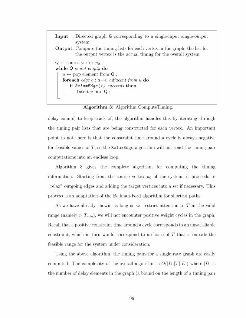
Input : Directed graph G corresponding to a single-input single-outputsystem
Output: Compute the timing lists for each vertex in the graph; the list forthe output vertex is the actual timing for the overall system
Q ← source vertex u0 ;while Q is not empty do
u ← pop element from Q ;foreach edge e : u→v adjacent from u do
if RelaxEdge( e) succeeds thenInsert v into Q ;
Algorithm 3: Algorithm ComputeTiming.
delay counts) to keep track of, the algorithm handles this by iterating through
the timing pair lists that are being constructed for each vertex. An important
point to note here is that the constraint time around a cycle is always negative
for feasible values of T , so the RelaxEdge algorithm will not send the timing pair
computations into an endless loop.
Algorithm 3 gives the complete algorithm for computing the timing
information. Starting from the source vertex u0 of the system, it proceeds to
“relax” outgoing edges and adding the target vertices into a set if necessary. This
process is an adaptation of the Bellman-Ford algorithm for shortest paths.
As we have already shown, as long as we restrict attention to T in the valid
range (namely > Tmin), we will not encounter positive weight cycles in the graph.
Recall that a positive constraint time around a cycle corresponds to an unsatisfiable
constraint, which in turn would correspond to a choice of T that is outside the
feasible range for the system under consideration.
Using the above algorithm, the timing pairs for a single rate graph are easily
computed. The complexity of the overall algorithm is O(|D||V ||E|) where |D| is
the number of delay elements in the graph (a bound on the length of a timing pair
96
list of a vertex), |V | is the number of vertices, and |E| is the number of edges in
the graph. Note that |D| is quite a pessimistic estimate, since it is very rare for
all the delays in a circuit to be on any single dominant path from input to output.
4.6 Multirate Systems
In this section, we consider some problems that arise in the treatment of multirate
systems. We examine some examples to see how these difficulties can be overcome,
and motivate new assumptions that make it easier to handle these systems
mathematically.
The conventional interpretation of SDF execution semantics has been based
on token counts on edges [66]. A vertex is enabled when each of its input edges
has accumulated a number of tokens greater than or equal to the consumption
parameter on that edge. At any time after it is enabled, the vertex may fire,
producing a number of tokens on each output edge equal to the production
parameter on that edge. In the following discussion, we use c to refer to the
consumption parameter on an edge, and p to refer to the production parameter.
The edge in question will be understood from the context.
This interpretation, though very useful in obtaining a strict mathematical
analysis of the consistency and throughput of such multirate systems, has some
unsatisfactory features when we consider dedicated hardware implementations.
One such feature is the fact that it results in tokens being produced in bursts
of p at a time on output edges and similarly consumed in bursts of c at a time.
Multirate algorithms may require the data rates on different edges to be different,
but this does not imply that the pattern of production is in bursts as implied
by the SDF model. This is, therefore, not necessarily the consumption pattern
97
implied in the design of DSP applications, where tokens refer to data samples on
edges, and as such will usually be strictly periodic at the sample rate specified for
that edge [43]. Moreover, in hardware designs at least, enforcing strict periodicity
on the samples means that any buffering required can be built into the consuming
unit and no special buffering needs to be provided for each edge.
A more important problem is with regard to the criterion used for firing
vertices. Consider the example of the 3 : 5 rate changer shown in Fig. 4.6.
According to the SDF interpretation, this vertex can only fire after 5 tokens are
queued on its input, and will then instantaneously produce 3 tokens on its output.
However, a real rate changer need not actually wait for 5 tokens before producing
its first output. In fact, in cases where such rate changers form part of a cycle in
the graph, the conventional interpretation can lead to deadlocked graphs due to
insufficient initial tokens on some edge, or even due to the distribution of tokens
among edges. One real life example where this criterion shows this problem is with
the DAT-to-CD data rate converter (used to convert between the data sample rates
used in Digital Audio Tape (DAT) and Compact Disc audio (CD)). This is a sample
rate conversion with a rate change ratio of 147 : 160. The SDF model interprets
this by saying that (when a DAT-CD converter is represented as a single block)
147 samples need to queue on the input before even a single output is produced,
and that all 160 corresponding outputs are produced together. This is clearly not
how it is implemented in practice, where a multiple stage conversion may be used,
or even in case of a direct conversion, the latency before producing the first output
does not need to be as high as indicated by the conventional SDF model. The
Cyclostatic dataflow (CSDF) [12] model provides a way around this by introducing
the concept of execution phases. We discuss the relation of our model to the CSDF
model in section 4.7.2.
98
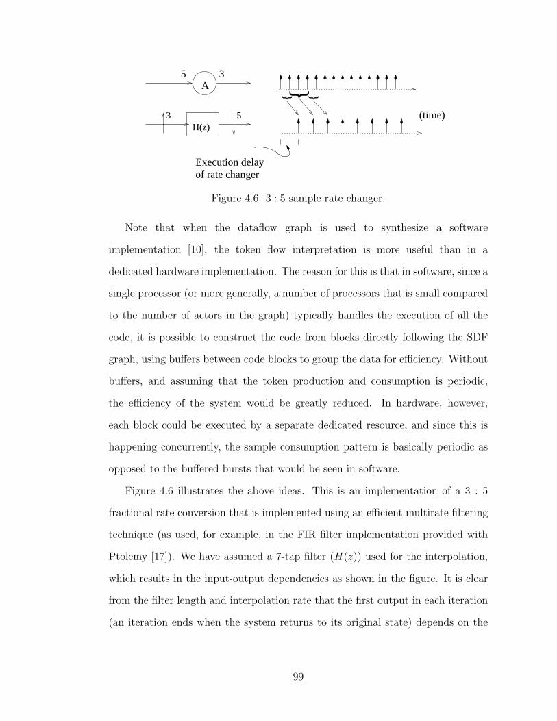
A5 3
(time)
Execution delayof rate changer
H(z)3 5
}} }
Figure 4.6 3 : 5 sample rate changer.
Note that when the dataflow graph is used to synthesize a software
implementation [10], the token flow interpretation is more useful than in a
dedicated hardware implementation. The reason for this is that in software, since a
single processor (or more generally, a number of processors that is small compared
to the number of actors in the graph) typically handles the execution of all the
code, it is possible to construct the code from blocks directly following the SDF
graph, using buffers between code blocks to group the data for efficiency. Without
buffers, and assuming that the token production and consumption is periodic,
the efficiency of the system would be greatly reduced. In hardware, however,
each block could be executed by a separate dedicated resource, and since this is
happening concurrently, the sample consumption pattern is basically periodic as
opposed to the buffered bursts that would be seen in software.
Figure 4.6 illustrates the above ideas. This is an implementation of a 3 : 5
fractional rate conversion that is implemented using an efficient multirate filtering
technique (as used, for example, in the FIR filter implementation provided with
Ptolemy [17]). We have assumed a 7-tap filter (H(z)) used for the interpolation,
which results in the input-output dependencies as shown in the figure. It is clear
from the filter length and interpolation rate that the first output in each iteration
(an iteration ends when the system returns to its original state) depends on the
99
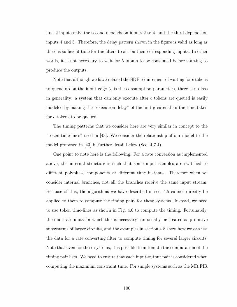
first 2 inputs only, the second depends on inputs 2 to 4, and the third depends on
inputs 4 and 5. Therefore, the delay pattern shown in the figure is valid as long as
there is sufficient time for the filters to act on their corresponding inputs. In other
words, it is not necessary to wait for 5 inputs to be consumed before starting to
produce the outputs.
Note that although we have relaxed the SDF requirement of waiting for c tokens
to queue up on the input edge (c is the consumption parameter), there is no loss
in generality: a system that can only execute after c tokens are queued is easily
modeled by making the “execution delay” of the unit greater than the time taken
for c tokens to be queued.
The timing patterns that we consider here are very similar in concept to the
“token time-lines” used in [43]. We consider the relationship of our model to the
model proposed in [43] in further detail below (Sec. 4.7.4).
One point to note here is the following: For a rate conversion as implemented
above, the internal structure is such that some input samples are switched to
different polyphase components at different time instants. Therefore when we
consider internal branches, not all the branches receive the same input stream.
Because of this, the algorithms we have described in sec. 4.5 cannot directly be
applied to them to compute the timing pairs for these systems. Instead, we need
to use token time-lines as shown in Fig. 4.6 to compute the timing. Fortunately,
the multirate units for which this is necessary can usually be treated as primitive
subsystems of larger circuits, and the examples in section 4.8 show how we can use
the data for a rate converting filter to compute timing for several larger circuits.
Note that even for these systems, it is possible to automate the computation of the
timing pair lists. We need to ensure that each input-output pair is considered when
computing the maximum constraint time. For simple systems such as the MR FIR
100
filter, inspection shows that the timing list is the same as that of an ordinary FIR
filter, possibly combined with some extra constant delay to take into account the
offset required for matching up the I-O for all the polyphase components.
The implementation we considered avoids unnecessary computations, so
it is possible to save power by either turning off the filters when they are
not needed (using the clock inputs), or by using an appropriate buffering
and delayed multiplication that will allow the multipliers to operate at 15
th
of the rate of the input stream, using the observation that only one of the
polyphase components [112] needs to operate for each output sample. This
tradeoff would depend on whether we are considering an implementation with
dedicated multipliers for each coefficient or shared multipliers. Real hardware
implementations of multirate systems must resort to such efficient realizations as
the performance penalties can otherwise be large.
The interpretation we use for execution of SDF graphs is therefore as follows:
each node receives its inputs in a perfectly periodic stream, and can start
computing its outputs some time after the first input becomes available (this time
would depend on internal features such as the number of taps in the filter in
the above example). The outputs are also generated in a periodic stream at the
appropriate rate required for consistency of the system.
An important effect of this alternate interpretation is that it changes the
criteria for deadlock in a graph. Under normal SDF semantics, the graph in
Fig. 4.7 would be deadlocked if the edge AB has less than 10 delays on it.
On the other hand, 6 delays are sufficient on edge BC, while 16 delays are
required on edge CA in order to prevent deadlock. The CSDF interpretation
mentioned in Sec. 4.7.2 tries to avoid these difficulties by prescribing different
token consumption and production phases, but introduces further complexity and
101
A
BC
4
5
3
23
10
n D
Figure 4.7 Deadlock in multirate SDF system: if n < 10 the graph deadlocks.
does not provide a complete solution to the timing problem. However, under our
new interpretation, as long as each cycle in the graph contains at least one token,
deadlock is broken and the system can execute. This is the same condition that
applies to homogeneous graphs.
It is important to understand that this interpretation of multirate SDF
execution is useful because dedicated hardware implementations of real multirate
DSP systems rarely require the interpretation in terms of token consumption of
the conventional SDF model. Typical multirate blocks in DSP applications are
decimators and interpolators (rate changers), multirate filters (very similar to rate
changers), serial-to-parallel converters and vice versa, block coders and decoders,
etc. A notable feature of these applications is that few of the applications actually
require a consumption of c tokens before starting to produce p tokens. Even for
block coders, in most implementations, for inter-operating with the rest of the
system, the data are produced in a periodic stream at a constant sample rate,
rather than in large bursts. As a result, the alternative interpretation of SDF
execution suggested above is efficient when targeting fixed hardware architectures.
102
4.6.1 HTP model for multirate systems
We now specify how the HTP model can be applied to the analysis of multirate
systems. We assume that the multirate system is specified in the SDF formulation.
For the execution semantics, we assume the data on each edge is periodic with a
relative sample rate determined by the SDF parameters, and the unit can begin
execution after the first input is received, instead of having to wait for c tokens.
Note that the second assumption can coexist with the conventional SDF
semantics. It is always possible to specify a timing delay for the unit that is greater
than the time required for c tokens to queue on the input edge. With this execution
time, we can be sure that the system will now satisfy traditional SDF semantics in
execution. However, in several cases, as pointed out previously, this is a pessimistic
requirement, and it is possible to choose a smaller delay that still provides enough
time for sufficient samples to be enqueued and for the appropriate computation
to occur. As long as we choose the timing delay such that for one period of the
samples there is sufficient time between consumption of input and production of
the output, the periodicity of the system will ensure that this constraint is met
for all successive periods.
For simplicity, we assume that the unit to be modeled is a SISO system and that
the propagation delay through sub-units is constant. The model can be extended
to handle more complicated units using a modification of the algorithms detailed
for homogeneous systems in Sec. 4.5.
Given a multirate system represented as an SDF graph, we follow the usual
technique [66] to compute the repetitions vector for the graph. The balance
equation on each edge e : u→v in the graph is given by
pe × qu = ce × qv, (4.3)
103
where pe is the production parameter on e, ce is the consumption parameter, and
qu and qv are the repetition counts for the source and sink of the edge. Let T
denote the overall iteration period of the graph. This is the time required for each
actor x to execute qx times (qx is the repetition count of the actor). Therefore,
the sample period on edge e is given by
Te =T
qu · pe
=T
qv · ce
. (4.4)
Now extending the analogy of the homogeneous case, we define the constraint
time on a path as
tc(p) =k∑
i=1
ti −k−1∑
j=1
(dj × Tj), (4.5)
where Tj is the sample period on edge j. By noting that the effect of a delay on
any edge (in both the homogeneous and multirate cases) is to give an offset of
−Te to the constraint time of any path through that edge, we can see that this
gives the correct set of constraints. Also, the values of the starting times for the
different vertices that are obtained as a solution to the set of constraints will give
a valid schedule for the multirate system.
It is possible to view the constraint times in terms of “normalized delays”.
Here the delays on each edge are normalized to a value of
dn(e) =de
qu · pe
=de
qv · ce
. (4.6)
In terms of the normalized delays, the expression for constraint time becomes the
same as that for the homogeneous case.
For homogeneous graphs, the minimum iteration period that can be attained
by the system is known as the iteration period bound and is known to be equal
to the maximum cycle-mean (MCM) [95, 60]. So far, no such tight bound is
known for multirate SDF graphs that does not require the costly conversion to
104
an expanded homogeneous equivalent graph. However, some good approximations
for multirate graphs have been proposed [101]. Under our model, it is easy to
determine an exact bound that is similar to the bound for homogeneous graphs,
but does not require the conversion to a homogeneous equivalent expanded graph.
By considering the cumulative constraints around a loop for the single rate case,
we can easily obtain the iteration period bound [95]
Tmin = maxc∈C
∑c tu∑c de
, (4.7)
where C is the set of all directed cycles in the graph.
Similarly, for the multirate case, we can obtain the result
Tmin = maxc∈C
∑c tu∑
c dn(e), (4.8)
where Tmin is the minimum admissible iteration period of the overall system as
discussed above. In addition, the start times for each operation are directly
obtained as a solution to the constraint system that is set up using the timing
information.
One factor here is that, unlike the homogeneous case, the number of timing
pairs in the list for a path is not bounded by the number of delay elements.
The denominator in a normalized delay is obtained as the product of a repetition
count of an actor and the consumption or production parameter for the edge
with the delay. As a result, on any path, the total normalized delay is the sum
of several terms with such denominators. The number of distinct such terms is
therefore bounded by the least common multiple of all these possible denominators.
However, in practice, it is rare for several such terms to exist in the timing pair
list, so this limit is very pessimistic. One reason for this is that if we consider two
paths between a pair of vertices such that one is dominated by the other, then
105
for all paths that pass through these two vertices, only the dominant path can
contribute to the timing pairs. Therefore, several paths are eliminated from the
possibility of contributing to a timing pair, and the size of the final timing list is
quite small. This is observed in the examples we have considered as well.
One possible source of misunderstanding in this context is the use of fractional
normalized delays in the computation. It may appear at first sight that the HTP
model allows fractional delays to be used in the graph even though such delays
have no physical meaning in the context of signal processing. In this context, it
is important to remember that the HTP model only specifies information about
the timing parameters of the graph. The functional correctness of the graph must
be verified by other means. In particular, any fractional normalized delays only
refer to the fact that the resulting timing shift is a fraction of an iteration period
interval, and does not indicate the use of actual fractional delays in a logical sense.
In the next section, we will look at how the HTP model for multirate dataflow
graphs stands in relation to other models that work with such systems, and then
present some examples of applying the model to represent timing for some well
known multirate applications in sec. 4.8.
4.7 Relation of the HTP Multirate Model to other Models
It is instructive to compare how the HTP model for multirate dataflow graphs
differs from some other models that have been proposed to deal with the difficulties
posed by the SDF execution semantics.
An important point worth noting is that although there have been previous
attempts (as described below) that have noticed the usefulness of fixing the exact
timing patterns, and of using strictly periodic timing patterns, none of these
106
approaches have developed these ideas into a timing model that is capable of
hierarchically representing complex sequential and multirate circuits.
4.7.1 Synchronous Reactive Systems
The HTP model proposed here is targeted towards describing the timing details
in an actual hardware implementation of the graph. As discussed in [9], there is
a distinction between the implementation dependent physical time consumption,
and the implementation independent logical synchronization. Models such as the
synchronous reactive systems described in [9] and the CSDF model discussed
below are in general more concerned with the implementation independent logical
synchronization and in verifying the functional correctness of the system. The
model we are proposing, on the other hand, is aimed at the “back-end” of the
synthesis process, that deals with the actual mapping to hardware and therefore
is concerned with implementation dependent timing parameters. In other words,
our model can be used in computing the actual performance metrics and the
implementation dependent issues after the functional correctness of the graph has
been verified by other means such as SR systems.
4.7.2 Cyclostatic Dataflow
Cyclostatic Dataflow (CSDF) [12] is an extension of SDF that introduces the
concept of “execution phases”. In this model, each edge has several execution
phases associated with it. In each phase, the sink vertex will consume a certain
number of tokens as specified by the consumption parameter of that phase for
that edge (similarly for the production on the source vertex of the edge). Over a
complete iteration, all phases of the edges are completed, and the system returns
107
to its original state. This is therefore a generalization of the SDF execution model.
It has been shown [12] that this model can avoid some of the deadlock issues that
affect the SDF model (such as in the example of fig. 4.7), by specifying the phases
at which the samples are consumed an produced.
The CSDF model is an execution model, not a timing model. As a result,
it leaves the exact time of execution of vertices free, and this is determined by
other means, such as run-time resolution of constraints, or construction of a static
schedule. The HTP model, on the other hand, is a timing model, and results in
static resolution of the times of execution. It also allows the computation of exact
values for performance metrics like the iteration period bound. In this sense, the
HTP model can in fact be used to complement the CSDF model, by making the
assumption that the different phases of execution occur periodically. However,
this is complicated a little by the fact that in the CSDF semantics, it is possible
for data coming out of a vertex to activate only some of its neighboring vertices in
certain phases and others in other phases. Because of this, the simple path based
constraint computation that we used to derive the timing pairs in the SDF model
may not be enough for CSDF. For example, in the case of the multirate FIR filter
(fig. 4.8), the different polyphase components do not receive the same data in an
efficient implementation (redundant computations are avoided). Furthermore, the
polyphase filter components receive their inputs at different phases of the input
clock. As a result, a time constraint that satisfies the relation between the first
output and its corresponding inputs may not satisfy the constraint between the
second output and its corresponding inputs. We can handle this situation by
inspection, and we can compute the timing pairs of the MR-FIR filter by hand,
and use this as a module in other systems such as filter banks. It is also possible
to automate this process to check all output phases and ensure that the time delay
108
is sufficient to satisfy all the timing constraints. The basic ideas of timing pairs
and timing pair lists that underly the HTP model still hold.
4.7.3 RT-level hardware timing model
Another model for timing of multirate hardware has been proposed by
Horstmannhoff, Grotker and Meyr [57]. They consider an alternative timing
model in which the samples occupy different phases of a master clock, and provide
interface circuitry to adjust the relative phases when samples are made available
on the edges. This requirement of a master clock means that the throughput is
already constrained and largely determined beforehand. The interface circuitry
can also be quite complex. Requiring a master clock to be specified also affects
the scalability of this approach: since the master clock is usually defined as the
least common multiple of local clocks, this can lead to a requirement for a very
fast master clock if the local clocks have relatively prime periods.
The model we propose tries to avoid these problems by not restricting itself to
cycle based timing. By enforcing periodicity on the data, it eliminates the need
for interface adjustments. An additional benefit of our model is that it allows the
iteration period of the system to be adjusted independently of any clock required
for cycle-based timing, and also gives an analytical solution for the best iteration
period that the system can attain.
4.7.4 Discrete Time domain in Ptolemy II
The work in [43] introduces the concept of “token time-line charts” with the
purpose of imposing the condition of strict periodicity on the flow of tokens between
actors in the dataflow model. This was found to be useful in understanding
109
discrete time domain implementations of the dataflow model (in the context
of the Ptolemy [17] system). However, this model still retains the token flow
interpretation of standard SDF by requiring the appropriate number of tokens to
be consumed and produced on each edge. As a result of this, the authors needed
to introduce initial “latency tokens” to avoid deadlock in certain situations.
The work in [43] resembles our model in the use of token time-lines with
periodic token flow. However, we have taken the idea further by relaxing the
token-flow interpretation of inter-actor communication, and used it to develop
a hierarchical model that can concisely represent timing in complex sequential
systems, as well as in multirate systems. This should allow the use of our model
for simplifying performance analysis of such complex systems.
4.8 Examples and Results
4.8.1 Multirate systems
We have applied the HTP model to the SDF graphs representing typical multirate
signal processing applications. The examples we have taken are from the Ptolemy
system [17] (CD-DAT, DAT-CD converters and 2 channel non-uniform filter bank)
and from [112, p.256] (tree-structured QMF bank).
The basic unit in several of these examples is the multirate FIR filter that is
capable of performing rate conversion as described in section 4.6. As noted there,
this must be treated as a primitive element of multirate systems. As shown in
Fig. 4.8, the implementation uses a certain number of internal filters corresponding
to the polyphase decomposition of the interpolating filter. We assume that these
are implemented in a manner similar to the filter shown on the left of Fig. 4.8, and
that the overall rate converting filter also therefore has similar timing parameters.
110
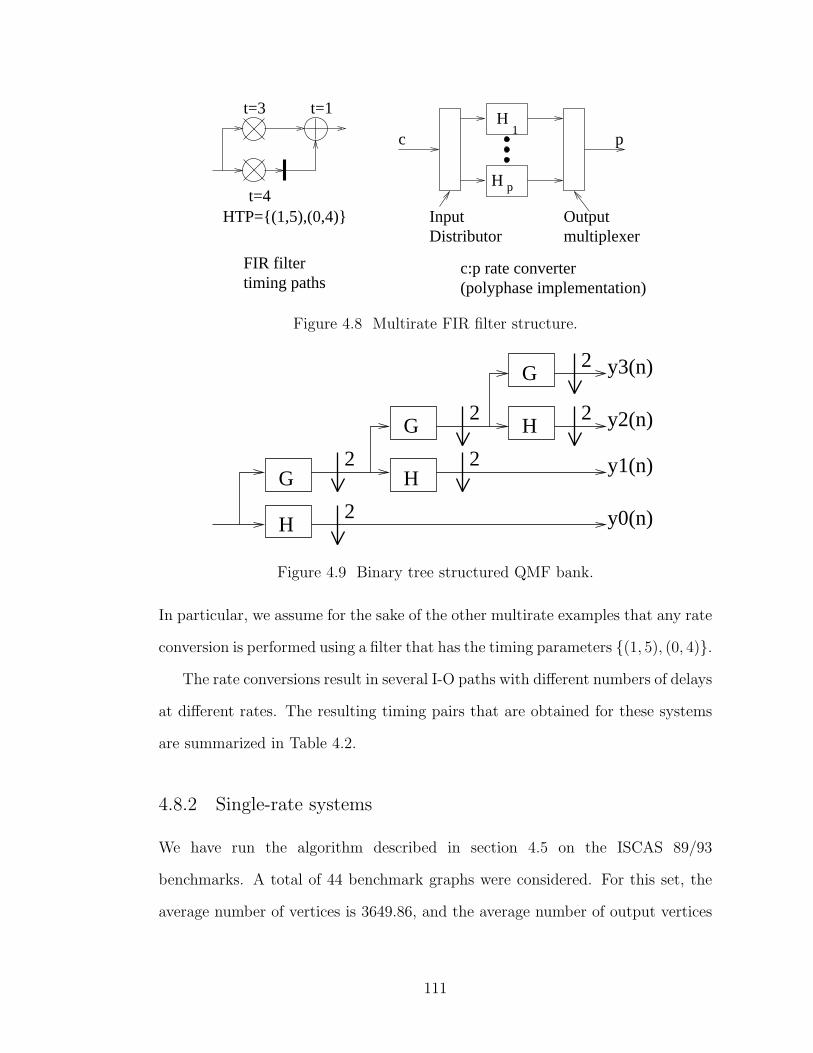
t=4
t=3 t=1
HTP={(1,5),(0,4)}
c p
Input Distributor
Outputmultiplexer
c:p rate converterFIR filtertiming paths
H1
H p
(polyphase implementation)
Figure 4.8 Multirate FIR filter structure.
2
2 2
2 2
2 y3(n)
y2(n)
y1(n)
y0(n)H
G H
G H
G
Figure 4.9 Binary tree structured QMF bank.
In particular, we assume for the sake of the other multirate examples that any rate
conversion is performed using a filter that has the timing parameters {(1, 5), (0, 4)}.The rate conversions result in several I-O paths with different numbers of delays
at different rates. The resulting timing pairs that are obtained for these systems
are summarized in Table 4.2.
4.8.2 Single-rate systems
We have run the algorithm described in section 4.5 on the ISCAS 89/93
benchmarks. A total of 44 benchmark graphs were considered. For this set, the
average number of vertices is 3649.86, and the average number of output vertices
111
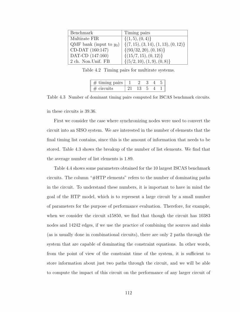
Benchmark Timing pairsMultirate FIR {(1, 5), (0, 4)}QMF bank (input to y3) {(7, 15), (3, 14), (1, 13), (0, 12)}CD-DAT (160:147) {(93/32, 20), (0, 16)}DAT-CD (147:160) {(15/7, 15), (0, 12)}2 ch. Non.Unif. FB {(5/2, 10), (1, 9), (0, 8)}
Table 4.2 Timing pairs for multirate systems.
# timing pairs 1 2 3 4 5# circuits 21 13 5 4 1
Table 4.3 Number of dominant timing pairs computed for ISCAS benchmark circuits.
in these circuits is 39.36.
First we consider the case where synchronizing nodes were used to convert the
circuit into an SISO system. We are interested in the number of elements that the
final timing list contains, since this is the amount of information that needs to be
stored. Table 4.3 shows the breakup of the number of list elements. We find that
the average number of list elements is 1.89.
Table 4.4 shows some parameters obtained for the 10 largest ISCAS benchmark
circuits. The column “#HTP elements” refers to the number of dominating paths
in the circuit. To understand these numbers, it is important to have in mind the
goal of the HTP model, which is to represent a large circuit by a small number
of parameters for the purpose of performance evaluation. Therefore, for example,
when we consider the circuit s15850, we find that though the circuit has 10383
nodes and 14242 edges, if we use the practice of combining the sources and sinks
(as is usually done in combinational circuits), there are only 2 paths through the
system that are capable of dominating the constraint equations. In other words,
from the point of view of the constraint time of the system, it is sufficient to
store information about just two paths through the circuit, and we will be able
to compute the impact of this circuit on the performance of any larger circuit of
112
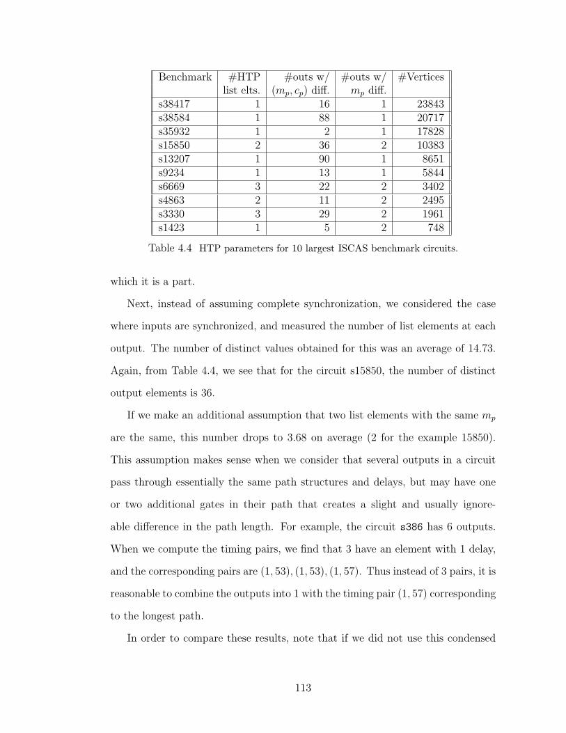
Benchmark #HTP #outs w/ #outs w/ #Verticeslist elts. (mp, cp) diff. mp diff.
s38417 1 16 1 23843s38584 1 88 1 20717s35932 1 2 1 17828s15850 2 36 2 10383s13207 1 90 1 8651s9234 1 13 1 5844s6669 3 22 2 3402s4863 2 11 2 2495s3330 3 29 2 1961s1423 1 5 2 748
Table 4.4 HTP parameters for 10 largest ISCAS benchmark circuits.
which it is a part.
Next, instead of assuming complete synchronization, we considered the case
where inputs are synchronized, and measured the number of list elements at each
output. The number of distinct values obtained for this was an average of 14.73.
Again, from Table 4.4, we see that for the circuit s15850, the number of distinct
output elements is 36.
If we make an additional assumption that two list elements with the same mp
are the same, this number drops to 3.68 on average (2 for the example 15850).
This assumption makes sense when we consider that several outputs in a circuit
pass through essentially the same path structures and delays, but may have one
or two additional gates in their path that creates a slight and usually ignore-
able difference in the path length. For example, the circuit s386 has 6 outputs.
When we compute the timing pairs, we find that 3 have an element with 1 delay,
and the corresponding pairs are (1, 53), (1, 53), (1, 57). Thus instead of 3 pairs, it is
reasonable to combine the outputs into 1 with the timing pair (1, 57) corresponding
to the longest path.
In order to compare these results, note that if we did not use this condensed
113

information structure, we would need to include information about each vertex
in the graph. In other words, in the best case, if we accept the (in most cases
justifiable) penalty for synchronizing inputs and outputs, we need to store an
average of 1.89 terms instead of 3649.86.
We have not considered the case of relaxing the assumptions on the inputs as
well. This would obviously increase the amount of data to be stored, but as we
have argued, our assumption of synchronized inputs and outputs has a very strong
case in its favor.
We have also computed the timing parameters for HLS benchmarks such as the
elliptic filter and 16-point FIR filter from [36]. These are naturally SISO systems,
which makes the synchronizing assumptions unnecessary. If we allow the execution
times of adders and multipliers to vary randomly, we find that the FIR filter has a
number of different paths which can dominate at different times. The elliptic filter
tends to have a single dominant path, but even this information is useful since it
can still be used to represent the filter as a single block.
A general observation we can make about the timing model is that systems that
have delay elements in the feed-forward section, such as FIR filters and filters with
both forward and backward delays, tend to have more timing pairs than systems
where the delay elements are restricted to a relatively small amount of feedback.
This is because feedback delay elements must necessarily exist in a loop that has
a total negative constraint time, which means they will not contribute towards a
dominant constraint time in the forward direction.
114
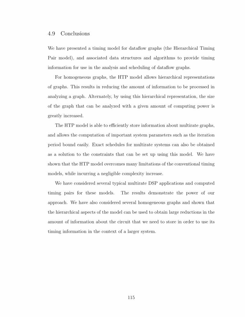
4.9 Conclusions
We have presented a timing model for dataflow graphs (the Hierarchical Timing
Pair model), and associated data structures and algorithms to provide timing
information for use in the analysis and scheduling of dataflow graphs.
For homogeneous graphs, the HTP model allows hierarchical representations
of graphs. This results in reducing the amount of information to be processed in
analyzing a graph. Alternately, by using this hierarchical representation, the size
of the graph that can be analyzed with a given amount of computing power is
greatly increased.
The HTP model is able to efficiently store information about multirate graphs,
and allows the computation of important system parameters such as the iteration
period bound easily. Exact schedules for multirate systems can also be obtained
as a solution to the constraints that can be set up using this model. We have
shown that the HTP model overcomes many limitations of the conventional timing
models, while incurring a negligible complexity increase.
We have considered several typical multirate DSP applications and computed
timing pairs for these models. The results demonstrate the power of our
approach. We have also considered several homogeneous graphs and shown that
the hierarchical aspects of the model can be used to obtain large reductions in the
amount of information about the circuit that we need to store in order to use its
timing information in the context of a larger system.
115

Chapter 5
Architecture synthesis search techniques
In chapter 3, we studied an efficient way to detect negative cycles in a graph,
with particular emphasis on the situation where the graph under consideration
is continuously changing with time (dynamic graphs). One possible application
mentioned there was the possibility of using design space exploration techniques
that make use of repeated computations of the negative cycle detection routine,
or the maximum cycle mean, in order to estimate the performance of a candidate
solution, and guide the development of better solutions.
In this chapter, we look at some algorithms for searching through the design
space that are based on these ideas. In particular, we are interested in designing
general optimization procedures that are able to handle multiple cost criteria. For
the most part, we will consider algorithms to minimize power consumption under
area and iteration period constraints, but will also look at how some of these
algorithms can be used to generate Pareto-optimal sets of solutions.
5.1 Deterministic local search
As we saw in chapter 2, several heuristics have been applied to the problem
of design space exploration. Most of these are designed with a single goal in
116

mind: for example, they try to minimize latency under a resource constraint,
or minimize resource consumption under a given latency constraint. When the
additional dimension of power reduction is introduced, the general scheduling
procedure becomes less easy to apply, and most approaches [99, 73] try to focus
on the problem of scheduling for low power on a fixed architecture, or with tight
architectural bounds (on the number of available resources).
Another approach to this is based on the idea of iterative improvement of
solutions, such as used, for example, in [90]. Here the idea is to have a synthesis
algorithm that performs an initial allocation, and then combine this with a series
of “moves” that have as their goal the improvement of the design characteristics.
The method used in [90] uses a standard scheduling algorithm at its core. Each
time a change is made to the scheduling decisions, or to the allocation of resources,
the entire transitive fanout of the affected vertex is rescheduled. For acyclic graphs
where the transitive fanout can only affect the final latency, and hence is equivalent
to a breadth-first search, it is possible to use such a technique effectively.
However, for cyclic graphs, the measure of the performance is not the end-
to-end latency, which can be computed using the breadth-first search described
above, but the maximum cycle mean, which could require a series of stages of
negative cycle detection with different iteration period estimates.
We propose a method for iterative module selection and scheduling based on
the idea of negative cycle detection. Once the modules have been selected and the
functions mapped onto them in order, the serialization of the vertices is finalized.
This means that we can now check the graph for the existence of negative timing
cycles, and if none such are present, we can conclude that the schedule is valid.
A similar approach of using the ordering to directly compute schedule times has
been used previously, for example see [113].
117
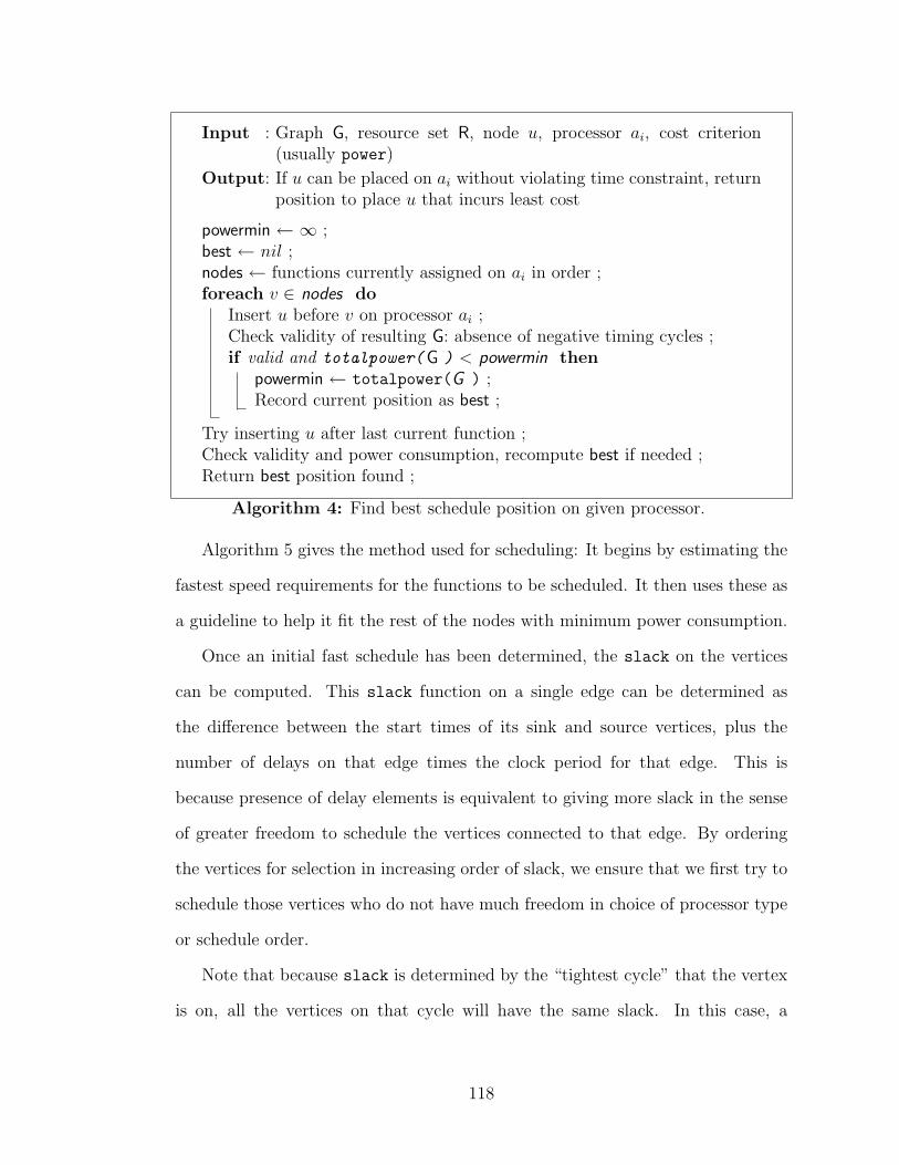
Input : Graph G, resource set R, node u, processor ai, cost criterion(usually power)
Output: If u can be placed on ai without violating time constraint, returnposition to place u that incurs least cost
powermin ← ∞ ;best ← nil ;nodes ← functions currently assigned on ai in order ;foreach v ∈ nodes do
Insert u before v on processor ai ;Check validity of resulting G: absence of negative timing cycles ;if valid and totalpower(G ) < powermin then
powermin ← totalpower(G ) ;Record current position as best ;
Try inserting u after last current function ;Check validity and power consumption, recompute best if needed ;Return best position found ;
Algorithm 4: Find best schedule position on given processor.
Algorithm 5 gives the method used for scheduling: It begins by estimating the
fastest speed requirements for the functions to be scheduled. It then uses these as
a guideline to help it fit the rest of the nodes with minimum power consumption.
Once an initial fast schedule has been determined, the slack on the vertices
can be computed. This slack function on a single edge can be determined as
the difference between the start times of its sink and source vertices, plus the
number of delays on that edge times the clock period for that edge. This is
because presence of delay elements is equivalent to giving more slack in the sense
of greater freedom to schedule the vertices connected to that edge. By ordering
the vertices for selection in increasing order of slack, we ensure that we first try to
schedule those vertices who do not have much freedom in choice of processor type
or schedule order.
Note that because slack is determined by the “tightest cycle” that the vertex
is on, all the vertices on that cycle will have the same slack. In this case, a
118
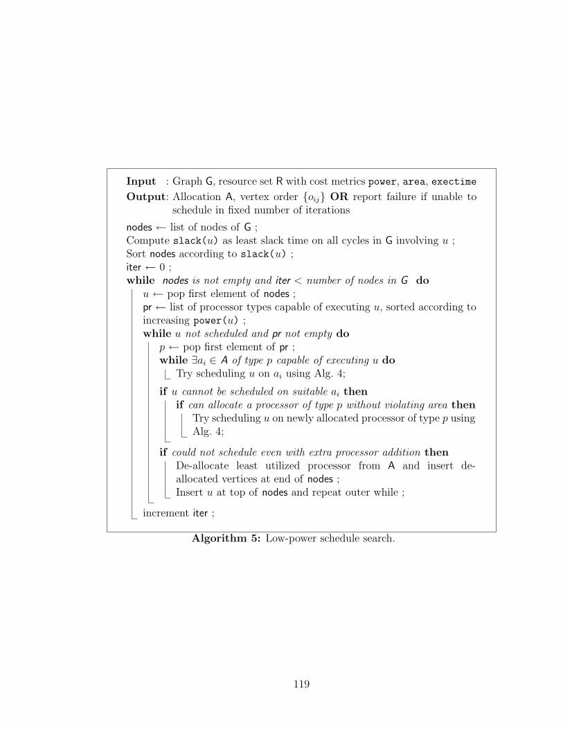
Input : Graph G, resource set R with cost metrics power, area, exectime
Output: Allocation A, vertex order {oij} OR report failure if unable toschedule in fixed number of iterations
nodes ← list of nodes of G ;Compute slack(u) as least slack time on all cycles in G involving u ;Sort nodes according to slack(u) ;iter ← 0 ;while nodes is not empty and iter < number of nodes in G do
u ← pop first element of nodes ;pr ← list of processor types capable of executing u, sorted according toincreasing power(u) ;while u not scheduled and pr not empty do
p ← pop first element of pr ;while ∃ai ∈ A of type p capable of executing u do
Try scheduling u on ai using Alg. 4;
if u cannot be scheduled on suitable ai thenif can allocate a processor of type p without violating area then
Try scheduling u on newly allocated processor of type p usingAlg. 4;
if could not schedule even with extra processor addition thenDe-allocate least utilized processor from A and insert de-allocated vertices at end of nodes ;Insert u at top of nodes and repeat outer while ;
increment iter ;
Algorithm 5: Low-power schedule search.
119
secondary sorting order based on power is used, so that vertices consuming the
largest amounts of power will be picked first for scheduling.
We now pick each vertex, and try to schedule it on an existing processor. We
choose the processors in increasing order of power consumption, so that in general
the system would first try its best to schedule on a processor of minimum power
consumption, before resorting to a higher power consumption processor. In this
way, it is making greedy decisions on the kind of processor to use, by trying to
focus on the least power processors. If no processor of the requested type has so far
been allocated, it tries to allocate a new processor, as long as the area constraint
is not violated.
If the algorithm cannot find any place for a particular vertex, this means that
we have over-allocated processors earlier, and possibly these are not being used
to their maximum capacity. So we define the utilization of a processor as the
ratio of the total time it is busy to the iteration period being targeted. Based on
this utilization, we then delete the processor that has the least utilization, and try
to re-schedule the other nodes.
Usually this whole process will terminate in a single sweep through the graph,
where appropriate processors are allocated and used to schedule all the vertices.
When the constraints are tight, however, we may need to go through the process of
deleting low utilization processors as described above. Since this could in general
be repeated indefinitely without leading to a correct result, we terminate the
algorithm after a certain number of iterations.
5.1.1 Fixed architecture systems
One variant of the low-power synthesis problem that has been studied in greater
depth in the literature ([91, 99, 73] is the case of scheduling on a fixed architecture.
120
The primary motivation in these cases has been to study how best to use the
availability of multiple supply voltages to reduce the power consumption, since
the power consumption varies as the square of the supply voltage, while the delay
(execution time) varies inversely as the supply voltage.
Note that this problem differs in a very important area from the case of full
architectural synthesis: allocation of resources is in itself a very complex task, so
assuming that we are already given a good allocation reduces the complexity of
the problem. However, it is still a useful special case to study, especially because it
is possible to use other techniques, such as genetic algorithms or other randomized
techniques, to evolve suitable allocations. This is possible since, as we will see
later in sec. 5.3.4, some of the difficulties in using GAs for schedule ordering can
be avoided if we only use the GA for module allocation and binding.
For the algorithm we have proposed in Alg. 5, the problem of scheduling on
a fixed architecture actually becomes somewhat simpler. We no longer have to
iterate through the process of deciding at each stage whether or not to add a new
processor, and we also do not need to deal with the problem of deleting processors
and re-scheduling them.
5.1.2 Experimental results
We have conducted experiments on scheduling some high-level synthesis
benchmarks using the algorithm suggested in the previous section. The
benchmarks for comparison are taken from [99]. Three benchmark circuits common
to the literature have been considered in this paper. The Elliptic filter example
has 26 add and 8 multiply operations. The AR filter has 12 add and 16 multiplies,
while the FIR filter has 15 add and 8 multiply operations. The resource library
is chosen such that a 5V adder takes 1 time step and consumes 52 = 25 units of
121
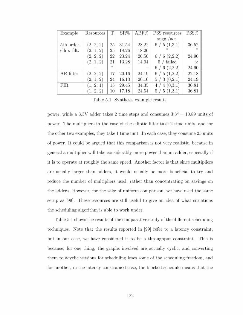
Example Resources T SR% ABF% PSS resources PSS%sugg./act.
5th order. (2, 2, 2) 25 31.54 28.22 6 / 5 (1,3,1) 36.52ellip. filt. (2, 1, 2) 25 18.26 18.26 ” ”
(2, 2, 2) 22 23.24 26.56 6 / 6 (2,2,2) 24.90(2, 1, 2) 21 13.28 14.94 5 / failed ×
– ” – – 6 / 6 (2,2,2) 24.90AR filter (2, 2, 2) 17 20.16 24.19 6 / 5 (1,2,2) 22.18
(2, 1, 2) 24 16.13 20.16 5 / 3 (0,2,1) 24.19FIR (1, 2, 1) 15 29.45 34.35 4 / 4 (0,3,1) 36.81
(1, 2, 2) 10 17.18 24.54 5 / 5 (1,3,1) 36.81
Table 5.1 Synthesis example results.
power, while a 3.3V adder takes 2 time steps and consumes 3.32 = 10.89 units of
power. The multipliers in the case of the elliptic filter take 2 time units, and for
the other two examples, they take 1 time unit. In each case, they consume 25 units
of power. It could be argued that this comparison is not very realistic, because in
general a multiplier will take considerably more power than an adder, especially if
it is to operate at roughly the same speed. Another factor is that since multipliers
are usually larger than adders, it would usually be more beneficial to try and
reduce the number of multipliers used, rather than concentrating on savings on
the adders. However, for the sake of uniform comparison, we have used the same
setup as [99]. These resources are still useful to give an idea of what situations
the scheduling algorithm is able to work under.
Table 5.1 shows the results of the comparative study of the different scheduling
techniques. Note that the results reported in [99] refer to a latency constraint,
but in our case, we have considered it to be a throughput constraint. This is
because, for one thing, the graphs involved are actually cyclic, and converting
them to acyclic versions for scheduling loses some of the scheduling freedom, and
for another, in the latency constrained case, the blocked schedule means that the
122

latency constraint is in fact the throughput of the system.
The columns in the table are explained below:
1. Example: The name of the example HLS benchmark circuit. The three
examples chosen, as explained above, are the elliptic wave filter, the AR
filter and a FIR filter section. The FIR filter is not truly a cyclic graph, but
our approach still exploits the fact that it is highly parallel, by allowing a
large degree of overlap between successive iterations.
2. Resources : The resource library consists of 3 element types: 5V adders, 3.3V
adders and 5V multipliers. The numbers in parentheses refer to the numbers
of each of these that are permitted in the system (5V +, 3.3V +, 5V×). The
same order is used in the later column on PSS resource selection (see below).
The multipliers take 2 units of time in the elliptic filter example and 1 unit
in the other 2, while the 5V adder takes 1 unit of time, and the 3.3V adder
takes 2 units of time in all cases.
3. T : This is the throughput constraint on the graph in time units. It is related
to the execution times of the resources as explained previously.
4. SR% : SR refers to the algorithm used in [99]. The number in this column
indicates the percentage of power savings obtained by using their algorithm
to schedule on the given resources.
5. ABF% : ABF refers to the algorithm for search we described above. It is
so called because it uses the Adaptive Bellman Ford algorithm for negative
cycle detection as the core of the schedule validation and search process.
This number is the percent power saving obtained using our search strategy.
123
6. PSS resources (sugg./ act.): PSS refers to the more general algorithm we
described above, where we also permit the algorithm to select the resources,
subject to an overall area constraint (PSS stands for Processor Selection and
Scheduling). This column shows the overall constraint we applied on this
scheduling strategy, along with the actual total resources that were consumed
by the algorithm. The numbers in parentheses represent the different types
of resources, as in the Resources column.
7. PSS% : This is the power saving obtained by using the PSS algorithm for
low-power scheduling.
Several interesting features can be noted from the results:
1. The ABF algorithm does considerably better than the SR algorithm on all
except one of the cases. This is partly because it makes use of the iterative
nature of the graph by implicitly allowing overlapped schedules.
2. The PSS algorithm is able to do even better than ABF on a number of
instances: this is because it is able to choose the resources, and therefore
is able to make a better determination, as in choosing 3 low-voltage adders
instead of 2 low-voltage and 1 high-voltage device.
3. The area trade-offs favor the PSS algorithm even more: in cases where it can
trade off a multiplier for an adder, our present comparison treats this as an
equal trade, whereas in reality the area savings will be considerable in such
a situation.
4. The PSS algorithm follows a greedy deterministic approach to scheduling,
and this shows in the fact that in certain situations, it actually fails to obtain
a schedule at all even though the constraints may not be very tight: this could
124
happen because it makes early decisions to use low-power processors, that
impact the schedulability of other functions down the line.
5. For the same reason, the ABF algorithm is able to outperform the PSS
algorithm: since it does not have to decide when and whether to add a
new processor, it seems to make fewer mistakes than the PSS algorithm in
obtaining schedules in some instances.
The results shown in Table 5.1 and the analysis above show that the algorithm
we have given has considerable promise for use in architectural synthesis. It is
simple to implement, yet quite efficient and able to find fairly good solutions. It
is also extremely fast running in practice, as all the examples shown (for graphs
with up to 34 vertices and 58 edges that were tried) were scheduled in a matter
of seconds on a medium range workstation (Pentium III 650 MHz, 192 MB RAM,
Windows 2000 operating system).
The failures of the algorithm shown in the table also indicate that there is room
for improvement: in general, it is very unlikely that a single deterministic algorithm
will ever be developed that can satisfactorily solve the architecture synthesis and
scheduling problem. Because of this, it becomes necessary to turn to randomized
algorithms, such as evolutionary techniques.
In the next section, we consider a genetic algorithm based on a simple
chromosome structure that uses the maximum cycle mean as a guide to derive
improved results. We will then also consider another algorithm based on the
range-chart guided scheduling algorithm [36]. Both these techniques are targeted
at evolving low-power architectures.
125
5.2 Genetic algorithms (GA)
Evolutionary algorithms [7, 52, 108, 116, 50] are a class of probabilistic techniques
that try to solve optimization problems. They are called evolutionary algorithms
because the main feature of the operation of the algorithm is that in all of these
techniques, certain features of the operation of the algorithm (either an encoding
of the potential solution, or other factors controlling the choice of solutions) is
“evolved” using operations such as crossover, mutation and reproductive selection
on a population of candidate solutions. There are several different types of EA,
such as evolutionary strategies [89], evolutionary programming [6] and genetic
algorithms. They each differ in the way they deal with the evolution of new
members of the population, and have shown their suitability in certain kinds of
tasks.
Genetic algorithms [56, 52, 50] are the most well known of the different types
of evolutionary algorithms. A genetic algorithm works on an encoding of the
parameters rather than on the parameter set itself. A population of candidate
solutions is generated (usually randomly, although it may be beneficial to seed
the population with known good solutions). The candidates from this population
are then evaluated to compute their fitness values. The fitness is a number that
indicates the relative merit of this particular solution compared to other solutions.
Based on the fitness values, a reproduction step is carried out, where members from
the population are chosen in such a way as to give preference to more fit solutions,
and the encodings for these solutions are crossed with each other to obtain a new
solution. Mutation is also used to introduce some randomness into the search. In
this way, a new population is obtained, that can then be put through the same
process iteratively. The process ends either after a fixed number of generations,
126
a fixed running time, or when the quality of solutions is found to converge to a
single value or a suitably small range of variation.
The main reason for the importance of genetic algorithms is, as mentioned
before, their robustness. They achieve this by means of a combination of several
factors: they work on an easily manipulatable coding of the solution space, use a
population of candidates for simultaneously exploring multiple possibilities, make
use of random operators, and utilize payoff information (in the form of fitness
values) to guide the evolution of better solutions, rather than using problem specific
methods to guide the search. This robustness allows them to be used in many
areas where optimization over a large multi-dimensional space is desired, with a
relatively easy to implement technique. In particular, they have found uses in
several areas of engineering usage [50, 52]. Recently there has been considerable
interest in applying them to problems in electronic design automation [108, 116],
because of the intractable nature of most of the optimization problems encountered
in this area.
In spite of the huge popularity and success of GAs in various engineering and
EDA fields, there are certain drawbacks and inefficiencies involved in using this
technique. In particular, when the application is to find a solution to a sequencing
or scheduling problem, a number of problems arise with respect to the proper
encoding of the parameters, and of the best definition of the crossover and mutation
operations in order to obtain the best solution. Although several approaches have
been proposed to meet these challenges, they often introduce other problems.
In the following sections, we will look at two genetic algorithms for the problem
of architecture synthesis and scheduling. These function quite well, and the
first application also demonstrates the power of adaptive negative cycle detection
techniques to speed up the search process. However, as will be noted, there
127
are problems with respect to the requirement that the chromosomes need to be
repaired before they are processed. This can be a computationally expensive
process, and can also lead to biasing of the search towards certain sections of the
search space. In section 5.4, we will present an alternative suggestion that tries
to avoid some of these problems, and could potentially be a useful new way of
looking at evolution techniques for architecture synthesis.
5.2.1 GA for architecture synthesis
For the purpose of our problem of architectural synthesis, we propose a fairly
simple GA encoding: the chromosome consists of 3 arrays of numbers as shown
in fig. 5.1. The first array ProcType is a list of resource types, indicating the
allocation of resources to this solution. It can have a variable length, thus changing
the total number of resources allocated to the system. In order to deal with possible
variations in the length of this chromosome, we can store the length of this array
as a part of the chromosome (NumProcs, and the crossover or mutation operators
will update it when they make changes to the array.
The next array is ProcMap. This is an array containing one element for
each vertex in the graph. The contents of the array are a number in the range
1 . . . NumProcs. The interpretation of this number is that the entry corresponding
to a given vertex decides the processor instance that the vertex maps to.
The final array is NodeLevel. This array can contain real values, and is used
to break ties in the ordering of vertices on a processor. That is, once the vertices
have been mapped to their processors using the ProcMap array, they need to be
ordered. A partial ordering is already imposed on them by the underlying graph,
but in general this leaves considerable freedom in the final ordering. In order to
ensure that all possible orderings are possible, we use a priority scheme that is
128
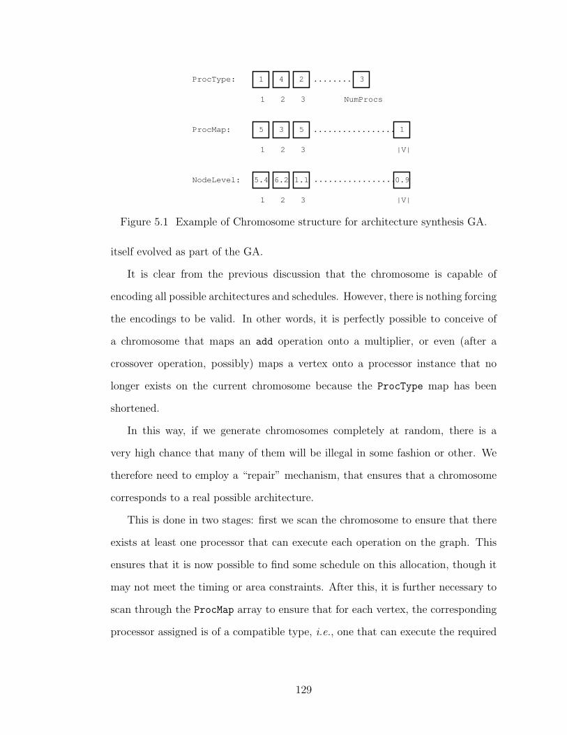
ProcType: 1 4 2 3........
1 2 3 NumProcs
ProcMap: 5 3 5 1.................
1 2 3 |V|
NodeLevel: 5.4 6.2 1.1 0.9
1 2 3 |V|
.................
Figure 5.1 Example of Chromosome structure for architecture synthesis GA.
itself evolved as part of the GA.
It is clear from the previous discussion that the chromosome is capable of
encoding all possible architectures and schedules. However, there is nothing forcing
the encodings to be valid. In other words, it is perfectly possible to conceive of
a chromosome that maps an add operation onto a multiplier, or even (after a
crossover operation, possibly) maps a vertex onto a processor instance that no
longer exists on the current chromosome because the ProcType map has been
shortened.
In this way, if we generate chromosomes completely at random, there is a
very high chance that many of them will be illegal in some fashion or other. We
therefore need to employ a “repair” mechanism, that ensures that a chromosome
corresponds to a real possible architecture.
This is done in two stages: first we scan the chromosome to ensure that there
exists at least one processor that can execute each operation on the graph. This
ensures that it is now possible to find some schedule on this allocation, though it
may not meet the timing or area constraints. After this, it is further necessary to
scan through the ProcMap array to ensure that for each vertex, the corresponding
processor assigned is of a compatible type, i.e., one that can execute the required
129
operation.
This repair mechanism needs to be employed at the initialization of the GA,
when the initial random population is generated. It also needs to be done at the
beginning of each iteration, in order to fix the chromosomes that have been newly
generated by the crossover and mutation operators. Apart from the additional
complexity introduced by this computation, there is also the danger of biasing
the search in the process of repairing the chromosome. This happens because
each time a chromosome is generated, we need to convert the invalid maps into
valid maps. If this is done deterministically, it means that several chromosomes
will map onto one chromosome, and the deterministic nature means that a few
chromosomes will be favored in this way, while others will never be mapped in this
fashion, and will only have their own basic representation for them. If we use a
non-deterministic repair mechanism, it means that it is possible to map a given
chromosome onto several different chromosomes, so we need to exercise care in
using a chromosome as a solution, because until it has been repaired, we cannot
truly see what it maps to.
The method of operation we use for the GA is as follows: the GA is first
initialized with a random population (repaired as explained above). Once these
candidates have been evaluated, they undergo a 2 element tournament selection
process (pick 2 at a time, one with better characteristics passes to next generation).
After selection, a number of rounds of crossover and mutation are applied, to
generate the new population. This process is repeated for a fixed number of
populations, determined empirically by the desire to run the GA for a reasonable
length of time and to allow a rough comparison against other probabilistic
algorithms. We also apply an elitist approach, by always retaining the best
solution to the next generation. This ensures that the GA will show continuous
130
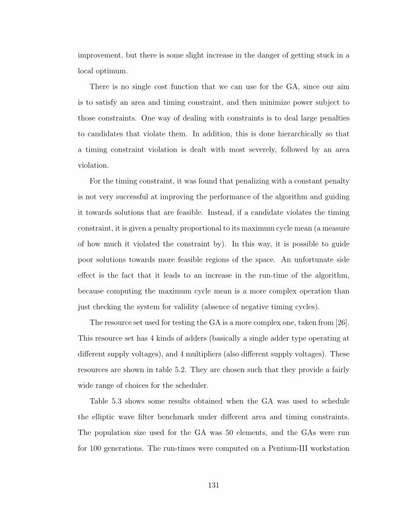
improvement, but there is some slight increase in the danger of getting stuck in a
local optimum.
There is no single cost function that we can use for the GA, since our aim
is to satisfy an area and timing constraint, and then minimize power subject to
those constraints. One way of dealing with constraints is to deal large penalties
to candidates that violate them. In addition, this is done hierarchically so that
a timing constraint violation is dealt with most severely, followed by an area
violation.
For the timing constraint, it was found that penalizing with a constant penalty
is not very successful at improving the performance of the algorithm and guiding
it towards solutions that are feasible. Instead, if a candidate violates the timing
constraint, it is given a penalty proportional to its maximum cycle mean (a measure
of how much it violated the constraint by). In this way, it is possible to guide
poor solutions towards more feasible regions of the space. An unfortunate side
effect is the fact that it leads to an increase in the run-time of the algorithm,
because computing the maximum cycle mean is a more complex operation than
just checking the system for validity (absence of negative timing cycles).
The resource set used for testing the GA is a more complex one, taken from [26].
This resource set has 4 kinds of adders (basically a single adder type operating at
different supply voltages), and 4 multipliers (also different supply voltages). These
resources are shown in table 5.2. They are chosen such that they provide a fairly
wide range of choices for the scheduler.
Table 5.3 shows some results obtained when the GA was used to schedule
the elliptic wave filter benchmark under different area and timing constraints.
The population size used for the GA was 50 elements, and the GAs were run
for 100 generations. The run-times were computed on a Pentium-III workstation
131
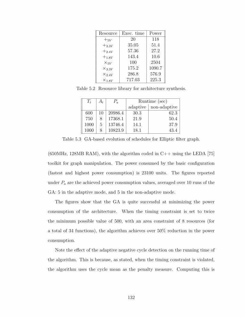
Resource Exec. time Power+5V 20 118+3.3V 35.05 51.4+2.4V 57.36 27.2+1.8V 143.4 10.6×5V 100 2504×3.3V 175.2 1090.7×2.4V 286.8 576.9×1.8V 717.03 225.3
Table 5.2 Resource library for architecture synthesis.
Tt At Pa Runtime (sec)adaptive non-adaptive
600 10 20986.4 30.3 62.3750 8 17368.1 21.9 50.41000 5 13746.4 14.1 37.91000 8 10823.9 18.1 43.4
Table 5.3 GA-based evolution of schedules for Elliptic filter graph.
(650MHz, 128MB RAM), with the algorithm coded in C++ using the LEDA [75]
toolkit for graph manipulation. The power consumed by the basic configuration
(fastest and highest power consumption) is 23100 units. The figures reported
under Pa are the achieved power consumption values, averaged over 10 runs of the
GA: 5 in the adaptive mode, and 5 in the non-adaptive mode.
The figures show that the GA is quite successful at minimizing the power
consumption of the architecture. When the timing constraint is set to twice
the minimum possible value of 500, with an area constraint of 8 resources (for
a total of 34 functions), the algorithm achieves over 50% reduction in the power
consumption.
Note the effect of the adaptive negative cycle detection on the running time of
the algorithm. This is because, as stated, when the timing constraint is violated,
the algorithm uses the cycle mean as the penalty measure. Computing this is
132
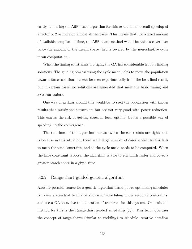
costly, and using the ABF based algorithm for this results in an overall speedup of
a factor of 2 or more on almost all the cases. This means that, for a fixed amount
of available compilation time, the ABF based method would be able to cover over
twice the amount of the design space that is covered by the non-adaptive cycle
mean computation.
When the timing constraints are tight, the GA has considerable trouble finding
solutions. The guiding process using the cycle mean helps to move the population
towards faster solutions, as can be seen experimentally from the best final result,
but in certain cases, no solutions are generated that meet the basic timing and
area constraints.
One way of getting around this would be to seed the population with known
results that satisfy the constraints but are not very good with power reduction.
This carries the risk of getting stuck in local optima, but is a possible way of
speeding up the convergence.
The run-times of the algorithm increase when the constraints are tight: this
is because in this situation, there are a large number of cases where the GA fails
to meet the time constraint, and so the cycle mean needs to be computed. When
the time constraint is loose, the algorithm is able to run much faster and cover a
greater search space in a given time.
5.2.2 Range-chart guided genetic algorithm
Another possible source for a genetic algorithm based power-optimizing scheduler
is to use a standard technique known for scheduling under resource constraints,
and use a GA to evolve the allocation of resources for this system. One suitable
method for this is the Range-chart guided scheduling [36]. This technique uses
the concept of range-charts (similar to mobility) to schedule iterative dataflow
133

graphs subject to timing or resource constraints. In particular, it can minimize
the resource usage for a given timing constraint.
This method suffers from some drawbacks, related to the fact that it requires
that execution times for all functions are a small integer number of clock cycles.
As a result, we need to convert the resource library shown in Table 5.2 to a
suitable format. This is done by setting the time of a 5V adder to 1 time unit, and
approximating the other units based on this. For example, a 3.3V adder is now 2
units, while a 5V multiplier is 5 time units. The algorithm takes time proportional
to the timing constraint it needs to meet, which means that for loose constraints,
it actually takes longer to schedule, than for tighter constraints.
For the purpose of the GA, we use a simple array that maps each vertex onto
a specific resource type. This fixes the execution time of the vertex, thereby
permitting the range-chart guided scheduling to work. This is now used to
minimize the resource constraint. In case of constraint violations, we penalize
the chromosome using fixed penalties.
This technique has some advantages over the other GA we used. In particular,
since the core scheduler has been designed specifically for resource constrained
scheduling, it is able to meet the timing constraints quite well in tight situations.
However, it takes longer for loosely constrained graphs, and the fact that it forces
the times of operations to be integers means that it loses some of the flexibility
that is possible in a complete self-timed schedule that can be obtained using the
other scheduling techniques.
The area minimization algorithm that is used here seems to have considerable
difficulty in tight situations. Although it meets the timing constraint by
constructing the schedule, it is trying to minimize the area rather than meet a
constraint directly. Because of the nature of the range chart guided scheduling
134
T A PRC20 PRC50 PABF tRC20(s) tRC50(s) tABF (s)600 10 20677.4 20118.4 20709.5 22.8 41.8 30.3750 8 17029.4 16395.2 17972.4 30.6 68.3 21.91000 5 16565.4 16327.0 13685.9 77.5 212.4 14.11000 8 10615.9 9093.6 10452.4 57.9 181.1 18.1
Table 5.4 Comparison of Range-chart guided GA vs. ABF based GA.
algorithm, it is not possible to use the resource constrained scheduler for our
purposes: since we are trying to construct an architecture, we do not know the
constraints on the different types of resources, only on the overall area.
Table 5.4 shows a comparison of the relative performances of the RC-guided
GA against the ABF based GA. We find that as far as the quality of the solutions
is concerned, they are very similar.
The columns labeled PRC50 and tRC50 present the power consumption and run-
time when the RC-guided GA is run for 100 iterations with a population size of
50, while PRC20 and tRC20 are the corresponding values for a population size of
20, and 100 iterations. The ABF algorithm is consistently faster, but for the lower
values of T (600 and 750) the difference is only a factor of 2-3 times for the same
number of generations. The performance is also quite similar, although we can
see that the RCGA with population of 50 consistently outperforms the GA with
a population of 20. A possible reason why we do not see large improvements by
more than doubling the population, is that once the GA gets close to the best
solution, the amount of improvement for a given investment of time reduces.
For T = 1000, with 2 different target areas, the results of the RCGA are
quite interesting. When the target area is a tight constraint (5), the GA has
considerable difficulty finding good solutions, and the power minimization is quite
poor compared to the other GA, especially taking into account that it runs for 10
times as long. When the area constraint is more relaxed, on the other hand, the
135
RCGA is able to do a very good job of finding power-efficient solutions.
The experiments reported so far show that the application of evolutionary
approaches to the architecture synthesis problem is quite promising, and we have
also seen ways of using the adaptive cycle mean computation to speed up the
operation of the algorithm.
However, the GAs still suffer from certain drawbacks: for example, the ABF
based GA requires a costly repair mechanism that could lead to bias in the solution
space if not treated carefully. In the next few sections, we will first look at one of
the features that make GAs useful, namely the idea of schemata or building blocks,
and then consider an approach to constructing schedules that tries to leverage this
idea.
5.3 Operating principle of Genetic algorithms
In this section, we examine some of the reasons for the success of GAs, and also
the reasons why they have difficulty in problems related to scheduling. Based on
these observations, we then propose some initial steps towards the possibility of a
better alternative to normal GAs that are better suited to synthesis problems.
5.3.1 Schemata
One of the most useful tools in understanding why GAs work is the concept of the
schema or similarity template [56, 52]. The idea behind a schema is to abstract
out part of a string encoding a solution as a template that contributes to the
utility of the solution. The most basic encoding for GAs is to encode the entire
representation in the form of a binary string (consisting of 1s and 0s). For example,
the encoding for a problem might involve a binary string of 7 elements. In such
136
a string, a pattern of the form *10**1* is an example of a schema. The schema
represents a part of the solution independent of the rest of the solution. Therefore,
for the above example, all encodings that contain 10 as the second and third
elements and 1 as the sixth element match the schema shown above. Here we can
also define two important metrics of the schema – the order of the schema is the
number of fixed locations in the schema (3 in this case), while the defining length
is the distance on the chromosome between the first and last fixed points of the
schema (in this case last position is 6, first position is 2, length is 6− 2 = 4).
The intuition behind the schema concept is that the overall solution for the
problem is actually made up of smaller solutions to parts of the problem. For the
case of an optimization, one can think of it in terms of dividing up the complete
problem into separate parts, optimizing each one independently, and putting them
together to obtain the best final solution. Of course, in reality it is not possible to
break up most optimization problems into sub-tasks in this fashion (the genetic
equivalent of this is termed epistasis). The nonlinear relations between different
parts of the chromosome due to epistasis mean that the contribution of a schema
to the overall fitness is actually strongly dependent on the rest of the chromosome.
However, assuming a certain degree of independence here allows us to gain some
insight into the working of the GA.
5.3.2 Fitness proportionate selection
GAs work by an iterative process of creating new generations of candidate
populations through crossover, mutation and reproductive selection. Of these,
the selection process determines how the GA retains good solutions and seeks out
better ones. The idea is that if a particular candidate solution has a high fitness,
then it is reasonable to assume that it is made up of smaller parts that in turn
137
conferred a certain degree of fitness on the overall solution. Therefore, by selecting
highly fit chromosomes for the purpose of crossover recombination to create the
next generation, we are giving more chances to those solutions that contain good
building blocks. These building blocks are essentially the same as the schemata
discussed in the previous section.
The reproductive schema growth equation [52] is an attempt at a mathematical
formulation of this idea. Consider a particular schema H, and assume that it
manifests itself by increasing the average fitness of all chromosomes containing that
schema. Let f be the average fitness of the overall population, and f(H) be the
average fitness of the elements containing this schema. Let m(H, t) and m(H, t+1)
denote the number of chromosomes containing the schema H at generations t and
t + 1 respectively.
Under these conditions, if we always choose chromosomes for reproduction with
a probability proportional to their fitness value, then the following relation holds:
m(H, t + 1) = m(H, t)f(H)
f.
In particular, assume that chromosomes containing the schema H remain above
average by an amount cf where c is a constant. Now m(H, t) can be written in
terms of the initial number of representatives m(H, 0) as
m(H, t) = m(H, 0)(1 + c)t.
This shows that the effect of fitness proportionate selection is to cause the
successful schema to increase and spread through the population exponentially.
Note that this is a very simplified view of the situation: in reality, it is not
usually true that a single schema by itself can increase the fitness of its chromosome
by a fixed factor; this would be very strongly dependent on the interaction with
138
other elements of the chromosome. Also, since the overall population fitness will
be improving with each generation, it is unlikely that the factor by which a single
schema increases the fitness will remain constant.
The effects of crossover and mutation on the selection process can also be taken
into account. From [52], the overall relation can be written as
m(H, t + 1) ≥ m(H, t) · f(H)
f· [1− pc
δ(H)
l − 1− o(H)pm].
Here pc is the probability of a crossover event, δ(H) is the defining length of the
schema H, l is the length of the chromosome, o(H) is the order of the schema, and
pm is the probability of a mutation event.
As we can see, crossover and mutation reduce the expected number of instances
of the schema, but their main purpose is to introduce new schema for analysis, so
as long as the rates of these operations are not so high as to disrupt the normal
operation of selection significantly, these terms do not play a very large role in the
fundamental operation of the GA.
5.3.3 Implicit parallelism
Apart from the exponential increase in number of good schemata, another factor
used to motivate the success of GAs is the number of schemata that can be
processed in each generation.
This problem has been analyzed in [52], with the result that the number of
schemata processed usefully per generation is estimated at O(n3), where n is the
size of the population. This indicates that the GA procedure of simultaneously
evaluating a large population and using these to generate the next population may
be capable of quite efficient processing of the schemata.
This is an optimistic estimate, for the following reasons:
139

1. n is the size of the population, and not, in general, related to the chromosome
length or complexity of the problem. It is usually chosen based on other
empirical studies.
2. To truly evaluate a schema completely, it is necessary to study the effect of
keeping this schema constant and averaging over all possible chromosomes.
The evaluation during one generation is, at best, an approximation to this.
3. Although O(n3) schemata are evaluated in each generation, they are not
necessarily distinct from one generation to the next.
5.3.4 Difficulties in using GAs for scheduling problems
Genetic algorithms work on an encoding of the solution, rather than the solution
itself. Because of this, the effectiveness of the search process depends on how good
the encoding is at capturing the features of the solution space. In particular, the
following features are desirable:
1. One-to-one mapping from encoding to solution: Mapping multiple
chromosomes to a single solution can lead to bias in the probability of finding
a particular solution. The reverse case of mapping a single chromosome to
multiple solutions introduces non-determinism, making it difficult to analyze
the effectiveness of the experiment.
2. Infeasible solution candidates : It is possible that some encodings map to
infeasible solutions. One way of dealing with this is to penalize such
solutions, but it would be desirable to avoid them in the first place.
3. Locality of the representation scheme [52, 40] : It is desirable that features
of a solution that depend closely on each other are encoded close to each
140
other, while features that are loosely interdependent can be further apart.
The success of operators such as crossover depends on this property.
4. Operator design: Suitable crossover and mutation operators must be
designed to fit the problem domain and yield good performance. Again,
this is not in general quantifiable, and a good localized string representation
would be preferable.
The problems in HLS include allocation of resources, binding of functions to
resources, and scheduling the functions on the resources. Of these, scheduling
is the most complex problem, but the combination proves even more difficult.
Several researchers have tried to use GAs to attack this problem. But there are
drawbacks associated with most approaches to applying GAs to the synthesis and
scheduling problem. The study of job-shop scheduling, which is a very similar
problem, encounters most of the same difficulties, and several techniques for these
problems are looked at in [50].
The main source of problems in the use of GAs is that scheduling is essentially
a sequencing problem: we want to find a sequence in which to order the operations
such that the overall system can meet certain performance constraints. The most
obvious approach for this would involve some kind of GA that directly encodes
the sequence of operations along with the processing element. The problem here
is that the normal crossover operator fails for sequences. Alternate methods such
as partially mapped crossover, cycle-based crossover [52] etc. have been proposed
and shown to be reasonably effective in a number of sequence related problems.
However, they are less intuitive than the original crossover operator.
An even greater problem in the case of scheduling is the existence of precedence
constraints among different functions in the graph. Because of this, not all
141
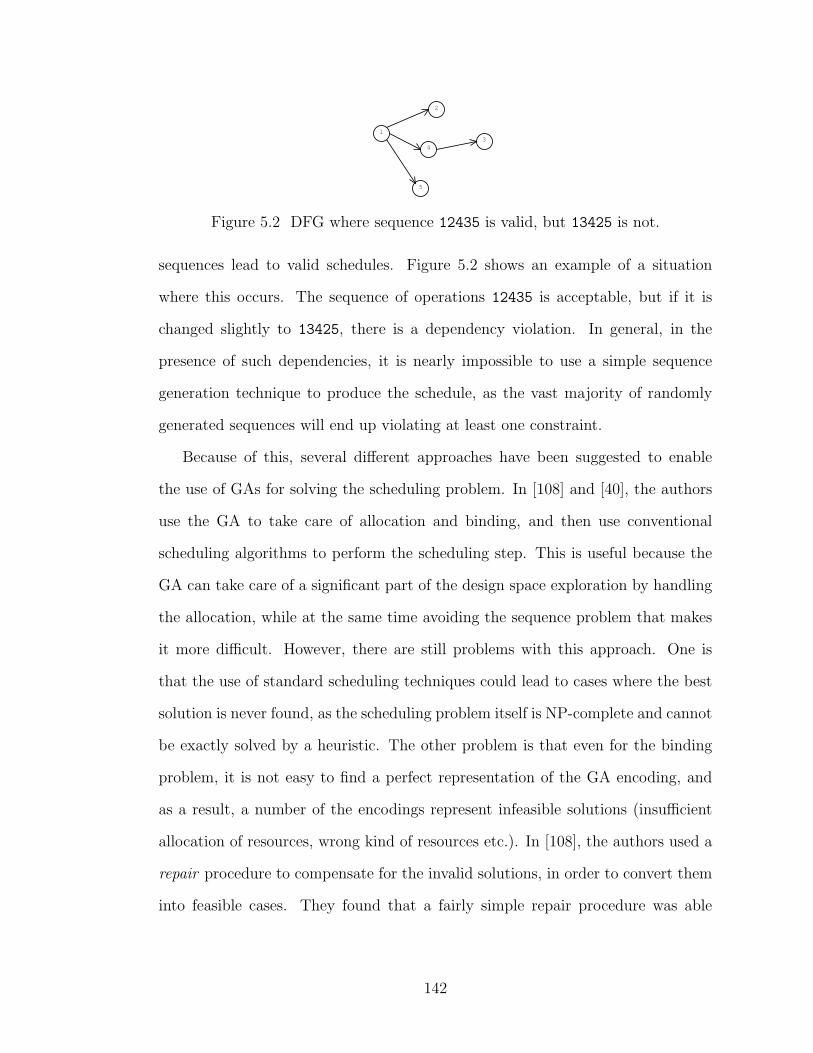
1
2
43
5
Figure 5.2 DFG where sequence 12435 is valid, but 13425 is not.
sequences lead to valid schedules. Figure 5.2 shows an example of a situation
where this occurs. The sequence of operations 12435 is acceptable, but if it is
changed slightly to 13425, there is a dependency violation. In general, in the
presence of such dependencies, it is nearly impossible to use a simple sequence
generation technique to produce the schedule, as the vast majority of randomly
generated sequences will end up violating at least one constraint.
Because of this, several different approaches have been suggested to enable
the use of GAs for solving the scheduling problem. In [108] and [40], the authors
use the GA to take care of allocation and binding, and then use conventional
scheduling algorithms to perform the scheduling step. This is useful because the
GA can take care of a significant part of the design space exploration by handling
the allocation, while at the same time avoiding the sequence problem that makes
it more difficult. However, there are still problems with this approach. One is
that the use of standard scheduling techniques could lead to cases where the best
solution is never found, as the scheduling problem itself is NP-complete and cannot
be exactly solved by a heuristic. The other problem is that even for the binding
problem, it is not easy to find a perfect representation of the GA encoding, and
as a result, a number of the encodings represent infeasible solutions (insufficient
allocation of resources, wrong kind of resources etc.). In [108], the authors used a
repair procedure to compensate for the invalid solutions, in order to convert them
into feasible cases. They found that a fairly simple repair procedure was able
142
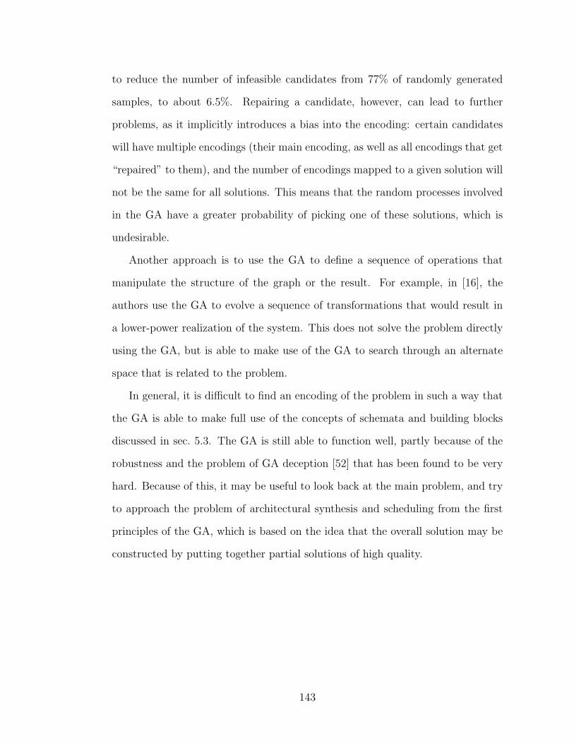
to reduce the number of infeasible candidates from 77% of randomly generated
samples, to about 6.5%. Repairing a candidate, however, can lead to further
problems, as it implicitly introduces a bias into the encoding: certain candidates
will have multiple encodings (their main encoding, as well as all encodings that get
“repaired” to them), and the number of encodings mapped to a given solution will
not be the same for all solutions. This means that the random processes involved
in the GA have a greater probability of picking one of these solutions, which is
undesirable.
Another approach is to use the GA to define a sequence of operations that
manipulate the structure of the graph or the result. For example, in [16], the
authors use the GA to evolve a sequence of transformations that would result in
a lower-power realization of the system. This does not solve the problem directly
using the GA, but is able to make use of the GA to search through an alternate
space that is related to the problem.
In general, it is difficult to find an encoding of the problem in such a way that
the GA is able to make full use of the concepts of schemata and building blocks
discussed in sec. 5.3. The GA is still able to function well, partly because of the
robustness and the problem of GA deception [52] that has been found to be very
hard. Because of this, it may be useful to look back at the main problem, and try
to approach the problem of architectural synthesis and scheduling from the first
principles of the GA, which is based on the idea that the overall solution may be
constructed by putting together partial solutions of high quality.
143
2
1 3
4
5
6 7
8
Figure 5.3 Example of a partial schedule.
5.4 Partial Schedules: Building blocks for architecture synthesis
Consider a final scheduled architecture for a DSP algorithm. It consists of
a number of processing elements, each of which has a number of functions
(corresponding to vertices in the dataflow graph), scheduled on it. The
act of scheduling the operations is equivalent to adding a certain number of
“serialization” edges to the graph, forcing those functions scheduled on the same
processor to execute in order.
We can abstract out this ordering into the concept of a partial schedule.
A partial schedule therefore represents a single processor, with the functions
scheduled on it. Given a partial schedule, the overall iteration period bound of
the system is now bounded from below by the sum of the execution times of the
vertices on this partial schedule. An overall schedule can then be constructed from
these partial schedules by combining appropriate partial schedules, making sure
that every vertex is represented exactly once, and no vertices are left out.
Example 5.1 Figure 5.3 shows an example of a partial schedule for a simple
dataflow graph. The graph corresponds to a second order filter section [36]. The
partial schedule is marked in grey, and the order of vertices on the partial schedule
is indicated by the arrows with dotted lines.
144
5.4.1 Features of partial schedules
In this section, we consider some of the useful features of the partial schedule
concept, and try to motivate the possibility of using them to build up an
architecture evolution system.
1. Infeasible orderings : By construction, partial schedules cannot contain any
infeasible edges. This makes sure that infeasibilities can arise only when we
combine different partial schedules. A drawback of this approach is that it
makes it difficult or impossible to propose a generic operator that combines
multiple partial schedules into a single one.
2. One-to-one mappings : Each partial schedule is uniquely defined, and by
using random generation techniques, they can be constructed without bias
towards any particular schedule.
3. Heterogeneous processing elements : The partial schedule is associated with
a processor type and list of vertices. In this way it simultaneously attacks
the problems of allocation, binding and scheduling, even for heterogeneous
processor systems.
4. Performance bounds : Each partial schedule automatically imposes a lower
bound on the performance of the complete schedule, given by the sum of
execution times of its functions. This can help to limit the search space and
improve the performance estimation.
5. Reduced equivalent graphs : Each partial schedule imposes a total ordering on
its vertices. Applying the HTP model (chapter 4) to this kind of a structure
is easier than for general graphs. In particular, it is possible to reduce the
chain of vertices in a partial schedule into a reduced graph corresponding to
145

only positions that have outputs followed by input edges. This can lead to
a 20-30% reduction in the size of the graph.
6. Intelligent generation of partial schedules : It is possible to use the output of
any other known algorithm as “seed” partial schedules. The search process
can then take over the task of combining these known partial schedules with
others to optimize other costs.
7. Pareto front construction: The nature of partial schedules makes it natural
to search the design space by combining them in different ways. This
automatically leads to the construction of a Pareto-optimal front [117], from
which we can then try to pick out the solutions that suit our needs best.
By constructing a pool of such partial schedules, it is possible to then search
through these to obtain a schedule that meets our requirements. The complexity of
this search is much less than a full combinatorial search through the design space.
In particular, for a population of N elements, it is reasonable to assume that if
the partial schedules are constructed at random, then we will see a distribution
of vertices to partial schedules such that the probability of a vertex being in any
random partial schedule is 12. In this situation, as soon as we choose one partial
schedule to construct our overall schedule, we can immediately eliminate all other
schedules that conflict with the vertices already scheduled on this.
The overall number of valid schedules that can then be constructed by searching
through such a pool of partial schedules can be estimated as follows: we assume
that if we pick a vertex at random, then it is present on average on half the
partial schedules. In this situation, choosing a vertex will eliminate N/2 of the
remaining partial schedules from consideration. At the next stage, a further half
of the remaining schedules will be eliminated, and so on. In this way, the number
146

of possible schedules can be estimated as
S(N) ≈ N
2× N
4× · · · × N
2i.
where S(N) is the number of valid schedules, N is the number of partial schedules
in the population, and i is the smallest integer such that 2i ≥ N . Since this gives
us
i = dlog2 Ne,
we can estimate
S(N) ≈ N log2 N .
For comparison, the entire search space that needs to be searched is of the order
of NN or even larger, because we have the problems of both choosing appropriate
resources, and finding a sequential ordering, which is O(N !) ≈ O(NN).
This function is more complex than a polynomial, but far less than the true
combinatorial number we would have to search if we wanted to search the entire
design space. Therefore, at least for reasonably sized instances, it may be possible
to use such a technique to search for schedules.
5.4.2 Drawbacks of partial schedules
We have proposed the idea of partial schedules as an attempt to provide a
representation of schedules that is more closely related to the actual structure
of schedules than a straightforward binary encoding in a string. The aim is to
then design a search process that uses this form of representation.
The partial schedules as proposed do a good job of capturing the concept of
building blocks that motivated the original GA design. Unfortunately, there are a
couple of problems with the representation that makes it difficult to construct a
useful GA around this representation.
147
The first problem relates to the “atomic” nature of partial schedules. Each
partial schedule fully captures the essence of one particular ordering. However,
there is no intuitive way to break a partial schedule into two smaller partial
schedules. In the other direction, there is no intuitive way to combine partial
schedules either.
As a result of this, it is not easy to define a crossover operator for partial
schedules, which combines partial schedules to generate better solutions. The
variation in the search process must then be introduced through the two processes
of random generation and mutation. In particular, it may be possible to use some
form of directed mutation rather than the blind mutation normally used in GAs.
The second major problem with partial schedules relates to the estimation of
fitness of a partial schedule. On one hand, the search process using the partial
schedules actually goes through all combinations of partial schedules with others.
In this way, we are evaluating each individual in its interaction with several other
individuals, and can obtain a better true estimate of the contribution of that
particular individual to the fitness of the overall system than in a typical GA
implementation.
The drawback is that it is not easy to compare the performance of different
individuals. The fact that a partial schedule was used in the construction of several
different final full schedules is an indicator that it is a useful unit, but may also
mean that it is just a very small unit that acts as a filler and so gets chosen often.
Because of this, it is not clear how exactly to reward or penalize a partial schedule
based on the performance of the final schedule.
148
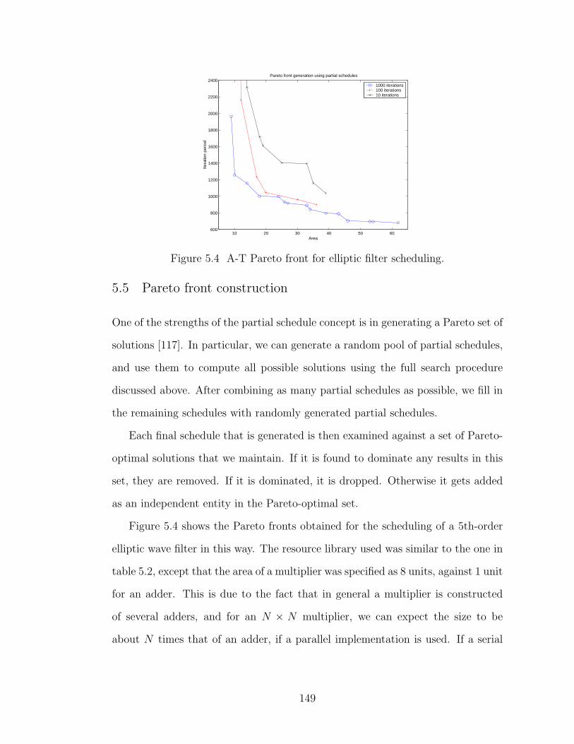
10 20 30 40 50 60600
800
1000
1200
1400
1600
1800
2000
2200
2400Pareto front generation using partial schedules
Area
Itera
tion
perio
d
1000 iterations100 iterations 10 iterations
Figure 5.4 A-T Pareto front for elliptic filter scheduling.
5.5 Pareto front construction
One of the strengths of the partial schedule concept is in generating a Pareto set of
solutions [117]. In particular, we can generate a random pool of partial schedules,
and use them to compute all possible solutions using the full search procedure
discussed above. After combining as many partial schedules as possible, we fill in
the remaining schedules with randomly generated partial schedules.
Each final schedule that is generated is then examined against a set of Pareto-
optimal solutions that we maintain. If it is found to dominate any results in this
set, they are removed. If it is dominated, it is dropped. Otherwise it gets added
as an independent entity in the Pareto-optimal set.
Figure 5.4 shows the Pareto fronts obtained for the scheduling of a 5th-order
elliptic wave filter in this way. The resource library used was similar to the one in
table 5.2, except that the area of a multiplier was specified as 8 units, against 1 unit
for an adder. This is due to the fact that in general a multiplier is constructed
of several adders, and for an N × N multiplier, we can expect the size to be
about N times that of an adder, if a parallel implementation is used. If a serial
149
implementation is used, then the size will be only slightly more than an adder,
but the execution time will be N times longer.
This problem is difficult for normal schedulers such as the range-chart guided
scheduling, because these systems first require the binding of functions to resources
to be specified, before they can proceed with scheduling. Figure 5.4 shows that
the partial schedule based search is able to find a continuous improvement in the
Pareto optimal front, and would allow us to choose an appropriate implementation
to meet our needs.
Another feature that can be noted from the construction is how often a partial
schedule is involved in the construction of a final good schedule. For the example
above, one sample run showed that after 100 generations, the Pareto optimal set
consisted of 10 points, made up of 53 distinct partial schedules. However, the
total number of partial schedules comprising the system was 152, meaning that
on average, each partial schedule was involved in 152/53 ≈ 3 final schedules that
were Pareto-optimal. More importantly, a single partial schedule was involved in
8 of the 10 Pareto points. This indicates that the idea of partial schedules as units
that contribute to the overall fitness has merit.
5.6 Conclusions
In this chapter, we have seen a number of ways in which to approach the problem of
architectural synthesis for iterative dataflow graphs. Existing approaches usually
target a single cost criterion, such as optimizing timing for a given resource
constraint, or vice versa. In addition, most of the existing techniques have been
developed for non-iterative graphs, thus making them inefficient when applied to
iterative graphs.
150
A deterministic search technique based on a greedy approach to minimizing
power consumption while trying to meet area and timing constraints was proposed.
This method can be applied both to the problem of arbitrary architecture selection,
as well as to scheduling under fixed architecture. The results of this method on
different kinds of HLS benchmarks show that it is able to obtain considerable
improvement over existing methods for low power scheduling even on fixed
architectures. Further, when it is given the freedom to select an architecture
subject to an overall area constraint, then it is able to outperform the existing low
power scheduling techniques by a large amount in most cases. The main drawback
of this approach is that the greedy approach sometimes tends to get it stuck in
certain local optima, which can lead to the overall solution being impossible to
find.
Another approach to scheduling that can avoid the problems of local optima is
to use probabilistic methods such as genetic algorithms. Two GAs were studied:
the first method is based on the idea of the GA generating the vertex ordering
– it uses the adaptive negative cycle detection approach to check the validity of
generated orders. The other approach uses the Range-chart guided scheduling
technique combined with a GA that generates the vertex to processor mapping.
Both these are quite effective at scheduling the system, but the range-chart guided
method is considerably more complex, and for the same population it takes a
considerably longer time to run. This results in the GA based on the ABF technique
being able to perform better when subject to an overall limit on the runtime.
In order to avoid some of the problems with GAs, in particular the problems
related to repair of chromosomes, a method of scheduling based on partial schedules
was proposed. Partial schedules are motivated by the idea of building blocks or
schemata that have been very useful in understanding the functioning of GAs.
151
By constructing a pool of partial schedules, it is possible to use an algorithm
that searches through these partial schedules to construct an overall schedule.
Some of the useful properties motivating the design and use of partial schedules
were considered. The application of partial schedules to Pareto-front generation
was shown. The partial schedule concept seems to hold promise in the area of
providing an efficient representation that can form the basis of evolutionary design
space exploration techniques.
152
Chapter 6
Conclusions and Future Work
This thesis has focused on three major areas of high level synthesis. In the following
sections, we present some of the main conclusions we draw from the results in each
of these areas, and some directions for future work.
6.1 Performance estimation
A new technique for detecting negative cycles in dynamic weighted digraphs was
presented. This method uses an adaptive variant of the Bellman-Ford algorithm
for shortest path computation in order to reduce the computation required to
detect negative cycles in cases where the underlying graph has undergone a small
number of changes. This dynamic situation arises in several problems in high level
synthesis, including performance estimation by calculation of the maximum cycle
mean, and design space exploration.
The algorithm we have presented is able to handle batches of changes made
to the underlying graph, as opposed to previous incremental approaches that only
handled one change at a time. When the changes occur in batches greater than
one, the incremental approach incurs a higher overhead as it has to analyze all
changes one at a time. The adaptive Bellman-Ford algorithm (ABF) that we have
153
presented, is able to check the feasibility of the constraints (detect negative cycles)
more efficiently by retaining values from previous iterations.
The ABF algorithm was compared against previous incremental approaches,
and shown to be superior even for fairly small batch sizes. An important
application of this method is in Lawler’s algorithm for computing the maximum
cycle mean as the performance bound of the system. By using this, significant
savings in the time required to compute the MCM were realized, and it was
shown that the resulting algorithm can outperform the fastest known algorithm
(Howard’s algorithm) for computing the MCM on sparse graphs such as are found,
for example in the ISCAS benchmark circuits.
6.1.1 Future directions
The analysis of the performance of the algorithm for negative cycle detection
currently indicates that it should be of the same order as the Bellman-Ford
algorithm, or O(V E) where V is the number of vertices and E is the number
of edges in the graph. For a sparse graph (E ≤ K × V for some constant K),
this becomes O(V 2). However, practical experiments show that in reality, this
quadratic behavior is never observed. The performance of the algorithm for sparse
graphs, except for pathological cases, is usually more like O(V ).
To see why this might be, note the following points about the Bellman-
Ford algorithm (Tarjan’s implementation of negative cycle detection – henceforth
referred to as the BFCT algorithm):
• The BFCT algorithm proceeds in at most V stages.
• If a vertex u has a shortest path from the source s that is of length ls(u) < V ,
then after the ls(u)th iteration, this vertex no longer changes its label.
154
From the above observations, it is clear that each vertex can be the source of a
“relaxation” operation (where all edges leaving it are examined and the sink labels
updated if necessary) at most ls(u) times. Since the out-degree is bounded by K,
this implies that a particular node can contribute at most K×ls(u) edge operations
to the execution of the algorithm. Therefore, the total number of operations
performed in the course of the algorithm is bounded above by K ×∑v∈V ls(v).
We would therefore like to find a bound on the expected value of LG =
∑v∈V ls(v). In [77], Moffat and Takaoka have proved that the average value of
LG = O(V log V ) for a complete graph, with edge weights in [0, 1]. However, it
is not easy to extend their proof to sparse graphs and general weights. A better
approach seems to be to follow the investigations of rumor spreading, as analyzed
by Pittel [87] for example.
Following these lines, it may be possible to show that the average case
performance of the negative cycle detection algorithm is O(V log V ) rather than
O(V 2). This would give a significant boost to the acceptability of the algorithm
for use in general situations involving such graphs.
6.2 Hierarchical timing representation
In chapter 4, a timing model for sequential and multirate iterative systems was
presented. The goal of this model is to provide a unified model that can encompass
normal combinational circuits (where it reduces to the longest path through
the circuit), single rate sequential circuits (where it is able to provide timing
information independent of the iteration period), and for multi-rate dataflow
graphs, where it provides analytical results for the performance bound similar
to single rate systems.
155
The model and algorithm were presented for both sequential and multirate
systems, and the computed results on benchmark circuits indicates that the model
has the potential for significantly reducing the amount of information that needs
to be stored in order to compute the timing constraints on the system.
For multirate systems, the model is able to account for different data rates
on different edges by accounting for time shifts that are a fraction of an iteration
interval. This formulation also allows us to use the maximum cycle mean with the
normalized delays as a bound on the iteration period of the system.
6.2.1 Future directions
Multirate systems HTP computation
The HTP model for multirate systems currently requires some amount of hand-
tuning to compute the values for the different parts of the graph. In particular,
as we saw in the multirate examples, the timing information for the basic filter
unit was computed by hand. This is necessary because the timing information for
the filter depends on the internal structure of the filter, and the instants at which
data are consumed and produced by the normal operation of the filter.
It would be preferable to be able to obtain this information automatically. This
may require more complicated analysis of the description of the filter unit. For
example, in a Verilog HDL description, it may be possible to note the timing cycles
at which data are consumed, and use this to estimate the timing of the multirate
filter.
156
Fixed phase registers
As was discussed in section 4.3.2, we assume that the delay elements in the circuit
are capable of being triggered at arbitrary instants. In general, in clocked circuits,
this is not very easy to implement. It would be interesting to see if the model can
be extended to the case where some or all of the registers are forced to trigger only
at certain time instants.
This idea is similar to the concept of mixed asynchronous synchronous
systems [109]. It may be possible to treat the system as consisting of some
synchronous units, which then communicate with each other using asynchronous
data transfer. The timing of a unit within a block would then be frozen relative
to the other units within that block, in some kind of a scheduling template [71].
This would considerably increase the range of applicability of the model.
Cyclostatic dataflow
Another interesting line of research would be to apply the HTP model to cyclostatic
dataflow graphs, as mentioned in sec. 4.7.2. This model naturally avoids some of
the problems of SDF regarding timing and deadlock. By combining this execution
model with the timing model provided by HTP, it should be possible to enrich the
understanding of both models.
The main complication in this, as mentioned in sec. 4.7.2, is the fact that
because cyclostatic systems work in phases, the longest path between two points
in the graph would pass through different vertices for different data inputs. It may
be possible to get around this by assigning an HTP timing list for each phase of the
input-output relation instead, but this requires further work to ensure correctness.
157
6.3 Architecture synthesis and scheduling
In chapter 5, we considered various approaches to the problem of architecture
synthesis. This problem is more complex than the simple scheduling problem
because we must first select an appropriate set of resources, and also perform the
scheduling on these resources. Since this means that we can obtain estimates of
the execution time of a function only after allocating a resource and binding the
function, it becomes difficult to use normal scheduling techniques that use timing
information for schedule construction.
We proposed methods based on a greedy search technique, as well as two
genetic algorithms, for solving this problem. It was shown that the GA based on
the use of the ABF algorithm is able to equal or outperform the GA based on
the range-chart guided scheduling method because of the improved run-times as a
result of the adaptive negative cycle detection.
A new representation of schedules in terms of combining partial schedules was
considered. This approach is inspired by the original working principle of the GA,
namely the idea of building a complex solution by combining simpler building
blocks. Partial schedules are an attempt to capture the idea of building blocks
used in GAs and work explicitly with them, rather than implicitly, as a GA does.
An application of this concept to the generation of a Pareto-front for architecture
synthesis was shown.
The design space covered by combining partial schedules in this fashion can be
searched much more efficiently than the entire system design space. The reason for
this, as shown in sec. 5.4.1, is that the conflicts between different partial schedules
naturally prunes the search space and reduces the complexity to O(Slog(S)) where
S is the number of partial schedules, as opposed to NN where N is the number
158
of vertices. Since S can be chosen as a reasonably small number and still cover
a large number of possibilities, this has the potential to increase the efficiency of
searching large design spaces.
6.3.1 Future directions
The partial schedule concept, as was shown in section 5.4.1, are able to capture
many of the important ideas behind the building block idea. However, in practice,
it is not clear how exactly to implement a consistent scheduling/search algorithm
that uses them successfully.
The current implementation uses randomly generated partial schedules,
together with some amount of directed mutation. It would be more suitable if
we could pinpoint what kind of improvements would benefit a partial schedule
most, and make it more useful in generating Pareto optimal solutions.
The problems mentioned in sec. 5.4.2 regarding the difficulties of applying
crossover and fitness estimation to partial schedules need to be examined more
closely. Without these operations, it is not possible to construct a useful GA,
although other forms of evolution not involving the crossover operator can still be
usefully applied.
Given the intrinsic ability of the approach to examine the entire Pareto front
in each iteration, it would be desirable to use this approach for multi-objective
optimization, rather than just two variable Pareto fronts as discussed in chapter 5.
159
BIBLIOGRAPHY
[1] R. K. Ahuja, T. L. Magnanti, and J. B. Orlin, Network Flows. Upper Saddle
River, NJ, USA: Prentice Hall, 1993.
[2] B. Alpern, R. Hoover, B. K. Rosen, P. F. Sweeney, and F. K. Zadeck,
“Incremental evaluation of computational circuits,” in Proc. 1st ACM-SIAM
Symposium on Discrete Algorithms, pp. 32–42, 1990.
[3] P. Ashenden, The Designer’s Guide to VHDL. San Francisco: Morgan
Kaufmann Publishers, 1995.
[4] J. Axelsson, “Architecture synthesis and partitioning of realtime systems: A
comparison of three heuristic search strategies,” in International Workshop
on Hardware-Software Codesign, (Braunschweig, Germany), Mar. 1997.
[5] S. Azarm, “Multiobjective optimum design: Notes.”
http://www.glue.umd.edu/˜azarm/optimum notes/multi/multi.html.
[6] T. Back, G. Rudolph, and H.-P. Schwefel, Proceedings of the Second Annual
Conference on Evolutionary Programming, ch. Evolutionary Programming
and Evolution Strategies: Similarities and Differences, pp. 11–22. San Diego,
CA: Evolutionary Programming Society, 1993.
160
[7] T. Back, U. Hammel, and H.-P. Schwefel, “Evolutionary computation:
Comments on the history and current state,” IEEE Transactions on
Evolutionary Computation, vol. 1, pp. 3–17, Apr. 1997.
[8] R. E. Bellman, “On a routing problem,” Quarterly Applied Mathematics,
vol. 16, pp. 87–90, 1958.
[9] A. Benveniste and G. Berry, “The synchronous approach to reactive and
real-time systems,” Proceedings of the IEEE, vol. 79, pp. 1270–1282, Sep
1991.
[10] S. S. Bhattacharyya, P. K. Murthy, and E. A. Lee, Software Synthesis from
Dataflow Graphs. Kluwer Academic Publishers, 1996.
[11] S. S. Bhattacharyya, S. Sriram, and E. A. Lee, “Resynchronization for
multiprocessor DSP systems,” IEEE Transactions on Circuits and Systems –
I: Fundamental Theory and Applications, vol. 47, pp. 1597–1609, November
2000.
[12] G. Bilsen, M. Engels, R. Lauwereins, and J. Peperstraete, “Cyclo-static
dataflow,” IEEE Transactions on Signal Processing, vol. 44, no. 2, pp. 397–
408, 1996.
[13] M. Boddy and T. L. Dean, “Solving timedependent planning problems,”
in Proceedings of the Eleventh International Joint Conference on Artificial
Intelligence, (Detroit, Michigan, USA), pp. 979–984, 1989.
[14] T. D. Braun et al., “A comparison of eleven static heuristics for mapping
a class of independent tasks onto heterogeneous distributed computing
161
systems,” Journal of Parallel and Distributed Computing, vol. 61, pp. 810–
837, 2001.
[15] F. Brglez, D. Bryan, and K. Kozminski, “Combinational profiles of sequential
benchmark circuits,” in Proc. IEEE Int. Symposium on Circuits and Systems
(ISCAS89), pp. 1929–1934, May 1989. ISCAS 89 Benchmarks.
[16] M. S. Bright and T. Arslan, “Synthesis of low-power dsp systems using a
genetic algorithm,” IEEE Transactions on Evolutionary Computation, vol. 5,
pp. 27–40, Feb. 2001.
[17] J. T. Buck, S. Ha, E. A. Lee, and D. G. Messerschmitt, “Ptolemy: A
framework for simulating and prototyping heterogeneous systems,” Int.
Jour. Computer Simulation, vol. 4, pp. 155–182, Apr 1994.
[18] Cadence Design Systems, Signal Processing Worksystem users manual. SPW
home page at http://www.cadence.com/products/spw.html.
[19] Cadence Design Systems, Inc., Cadence Design Systems Users manual.
Cadence home page at http://www.cadence.com/products/sld.html.
[20] N. Chandrachoodan, S. S. Bhattacharyya, and K. J. R. Liu, “Adaptive
negative cycle detection in dynamic graphs,” in Proceedings of International
Symposium on Circuits and Systems (ISCAS 2001), vol. V, (Sydney,
Australia), pp. 163–166, May 2001.
[21] N. Chandrachoodan, S. S. Bhattacharyya, and K. J. R. Liu, “An efficient
timing model for hardware implementation of multirate dataflow graphs,” in
Proceedings of the International Conference on Acoustics, Speech, and Signal
Processing (ICASSP 2001), (Salt Lake City, Utah), May 2001.
162
[22] N. Chandrachoodan, S. S. Bhattacharyya, and K. J. R. Liu, “The
hierarchical timing pair model,” in Proceedings of International Symposium
on Circuits and Systems (ISCAS 2001), vol. V, (Sydney, Australia), pp. 367–
370, May 2001.
[23] N. Chandrachoodan, S. S. Bhattacharyya, and K. J. R. Liu, “Negative cycle
detection in dynamic graphs,” Tech. Rep. UMIACS-TR-99-59, University
of Maryland Institute for Advanced Computer Studies, September 1999.
http://dspserv.eng.umd.edu/pub/dspcad/papers/.
[24] A. Chandrakasan, M. Potkonjak, J. M. Rabaey, and R. W. Brodersen,
“HYPER-LP: a system for power minimization using architectural
transformations,” in Proceedings of Int. Conf. on Comp. Aided Design
(ICCAD 92), pp. 300–303, 1992.
[25] A. Chandrakasan and R. Brodersen, “Minimizing power consumption in
digital CMOS circuits,” Proceedings of the IEEE, vol. 83, pp. 498–523, 1995.
[26] J. Chang and M. Pedram, “Energy minimization using multiple supply
voltages,” in ISLPED ’96, (Monterey, CA), pp. 157–162, ACM, Aug 1996.
[27] D. Y. Chao and D. T. Wang, “Iteration bounds of single rate dataflow graphs
for concurrent processing,” IEEE Transactions on Circuits and Systems - I,
vol. 40, pp. 629–634, Sep 1993.
[28] L. F. Chao and E. H. M. Sha, “Retiming and clock skew for synchronous
systems,” in Proceedings of the International Symposium on Circuits and
Systems (ISCAS 94), vol. 1, pp. 283–286, 1994.
163
[29] B. Cherkassky and A. V. Goldberg, “Negative cycle detection algorithms,”
Tech. Rep. tr-96-029, NEC Research Institute, Inc., March 1996.
[30] F. Cieslok and J. Teich, “Timing analysis of process models with uncertain
behaviour,” date-report num. 1/00, DATE, University of Paderborn, 2000.
[31] J. Cochet-Terrasson, G. Cohen, S. Gaubert, M. McGettrick, and J.-P.
Quadrat, “Numerical computation of spectral elements in max-plus algebra,”
in Proc. IFAC Conf. on Syst. Structure and Control, 1998.
[32] T. H. Cormen, C. E. Leiserson, and R. L. Rivest, Introduction to Algorithms.
Cambridge, MA: MIT Press, 1990.
[33] G. B. Dantzig, Linear Programming and Extensions. Princeton, New Jersey,
USA: Princeton University Press, 1963.
[34] A. Dasdan, S. S. Irani, and R. K. Gupta, “An experimental study of
minimum mean cycle algorithms,” Tech. Rep. UCI-ICS #98-32, Univ. of
California Irvine, 1998.
[35] A. Dasdan, S. S. Irani, and R. K. Gupta, “Efficient algorithms for optimum
cycle mean and optimum cost to time ratio problems,” in 36th Design
Automation Conference, pp. 37–42, ACM/IEEE, 1999.
[36] S. M. H. de Groot, S. H. Gerez, and O. E. Herrmann, “Range-chart-guided
iterative data-flow graph scheduling,” IEEE Transactions on Circuits and
Systems - I, vol. 39, pp. 351–364, May 1992.
[37] G. de Micheli, Synthesis and Optimization of Digital Circuits. McGraw Hill,
1994.
164
[38] T. L. Dean and M. Boddy, “An analysis of timedependent planning,” in
Proceedings of the Seventh National Conference on Artificial Intelligence,
(Minneapolis, MN, USA), pp. 49–54, 1988.
[39] S. Devadas and R. Newton, “Algorithms for hardware allocation in data path
synthesis,” IEEE Transactions on Computer Aided Design, vol. 8, pp. 768–
781, July 1989.
[40] R. P. Dick and N. K. Jha, “MOGAC: A multiobjective genetic algorithm
for hardware-software co-synthesis of distributed embedded systems,” IEEE
Transactions on Computer Aided Design, vol. 17, no. 10, pp. 920–935, 1998.
[41] H. A. Eschenauer, J. Koski, , and A. Osyczka, Multicriteria Design
Optimization : Procedures and Applications. New York: Springer-Verlag,
1986.
[42] J. P. Fishburn, “Clock skew optimization,” IEEE Transactions on
Computers, vol. 39, pp. 945–951, Jul 1990.
[43] C. Fong, “Discrete-time dataflow models for visual simulation in Ptolemy
II,” Master’s thesis, University of California, Berkeley, Dec. 2000.
[44] L. Ford, “Network flow theory,” Tech. Rep. P-932, The Rand Corporation,
1956.
[45] D. Frigioni, M. Ioffreda, U. Nanni, and G. Pasqualone, “Experimental
analysis of dynamic algorithms for single source shortest paths problem,”
in Proc. Workshop on Algorithm Engineering (WAE ’97), 1997.
[46] D. Frigioni, A. Marchetti-Spaccamela, and U. Nanni, “Fully dynamic
shortest paths and negative cycle detection on digraphs with arbitrary arc
165
weights,” in ESA98, vol. 1461 of Lecture Notes in Computer Science, (Venice,
Italy), pp. 320–331, Springer, August 1998.
[47] M. R. Garey and D. S. Johnson, Computers and Intractability - A guide
to the theory of NP-completeness. W.H.Freeman and Company, NY, USA,
1979.
[48] C. H. Gebotys and M. I. Elmasry, “Simultaneous scheduling and allocation
for cost constrained optimal architectural synthesis,” in 28th DAC, 1991.
[49] R. Geiger, P. Allen, and N. Strader, Design Techniques for Analog and
Digital Circuits. McGraw-Hill series in Electronic Engineering, McGraw-
Hill, 1990.
[50] M. Gen and R. Cheng, Genetic Algorithms and Engineering Design. Wiley
series in Engineering Design and Automation, Wiley-Interscience, 1997.
[51] S. H. Gerez, S. M. H. de Groot, and O. E. Hermann, “A polynomial time
algorithm for computation of the iteration period bound in recursive dataflow
graphs,” IEEE Transactions on Circuits and Systems - I, vol. 39, pp. 49–52,
Jan 1992.
[52] D. Goldberg, Genetic Algorithms in Search, Optimization and Machine
Learning. Reading, MA: Addison-Wesley, 1989.
[53] P. Groeneveld and P. Stravers, Ocean: the Sea-of-Gates Design System
Users Manual. Delft University of Technology, Delft, the Netherlands, 1994.
http://cas.et.tudelft.nl/software/ocean/ocean.html.
166
[54] P. L. Guernic, T. Gautier, M. le Borgne, and C. le Maire, “Programming real-
time applications with SIGNAL,” Proceedings of the IEEE, vol. 79, pp. 1321–
1336, Sep 1991.
[55] D. Harel, “Statecharts: A visual approach to complex systems,” Science of
Computer Programming, vol. 8, pp. 231–274, 1987.
[56] J. H. Holland, Adaptation in natural and artificial systems. Ann Arbor, MI,
USA: The University of Michigan Press, 1975.
[57] J. Horstmannshoff, T. Grotker, and H. Meyr, “Mapping multirate dataflow
to complex RT level hardware models,” in ASAP ’97, 1997.
[58] T. C. Hu, Integer programming and network flows. Reading, Mass., USA:
Addison-Wesley Publishing Co., 1970.
[59] Institute of Electrical and Electronic Engineers, Standard VHDL Language
Reference Manual, IEEE 1076-1993, 1993.
[60] K. Ito and K. K. Parhi, “Determining the minimum iteration period of an
algorithm,” Journal of VLSI Signal Processing, vol. 11, pp. 229–244, 1995.
[61] H. V. Jagadish and T. Kailath, “Obtaining schedules for digital systems,”
IEEE Transactions on Signal Processing, vol. 39, pp. 2296–2316, Oct 1991.
[62] V. Kianzad and S. S. Bhattacharyya, “Multiprocessor clustering for
embedded systems,” in Proceedings of the European Conference on Parallel
Computing, (Manchester, United Kingdom), pp. 697–701, Aug. 2001.
[63] N. Kobayashi and S. Malik, “Delay abstraction in combination logic
circuits,” IEEE Transactions on Computer Aided Design, vol. 16, pp. 1205–
1212, Oct. 1997.
167
[64] E. Lawler, Combinatorial Optimization: Networks and Matroids. New York:
Holt, Rhinehart and Winston, 1976.
[65] E. L. Lawler, “Fast approximation schemes for knapsack problems,” in Proc.
18th Ann. Symp. on Foundations of Computer Science, pp. 206–13, IEEE
Computer Soc., 1977.
[66] E. A. Lee and D. G. Messerschmitt, “Synchronous data flow,” Proceedings
of the IEEE, vol. 75, pp. 1235–1245, Sep 1987.
[67] C. E. Leiserson and J. B. Saxe, “Retiming synchronous circuitry,”
Algorithmica, vol. 6, pp. 5–35, 1991.
[68] Y.-R. Lin, C.-T. Hwang, and A. C.-H. Wu, “Scheduling techniques
for variable voltage low power designs,” ACM Transactions on Design
Automation of Embedded Systems, vol. 2, pp. 81–97, Apr 1997.
[69] K. Liu, A.-Y. Wu, A. Raghupathy, and J. Chen, “Algorithm-based low-
power and high-performance multimedia signal processing,” Proceedings of
the IEEE, vol. 86, pp. 1155–1202, 1998.
[70] L.-T. Liu, M. Shih, J. Lillis, and C.-K. Cheng, “Data-flow partitioning with
clock period and latency constraints,” IEEE Transactions on Circuits and
Systems - I, vol. 44, Mar 1997.
[71] T. Ly, D. Knapp, R. Miller, and D. MacMillen, “Scheduling using behavioral
templates,” in Proceedings of 32nd Design Automation Conference, (San
Francisco, CA), ACM/IEEE, June 1995.
[72] N. Maheshwari and S. S. Sapatnekar, “Efficient retiming of large circuits,”
IEEE Transactions on VLSI Systems, vol. 6, pp. 74–83, Mar 1998.
168
[73] A. Manzak and C. Chakrabarti, “A low-power scheduling scheme with
resources operating at multiple voltages,” in Proceedings of the International
Symposium on Circuits and Systems, ISCAS 99, pp. 354–357, IEEE, 1999.
[74] C. Mead and L. Conway, Introduction to VLSI systems. Reading, Mass.:
Addison-Wesley, 1980.
[75] K. Mehlhorn and S. Naher, “LEDA: A platform for combinatorial and
geometric computing,” Communications of the ACM, vol. 38, no. 1, pp. 96–
102, 1995.
[76] G. D. Micheli, D. Ku, F. Mailhot, and T. Truong, “The olympus synthesis
system for digital design,” IEEE Design and Test, pp. 37–53, 1990.
[77] A. Moffat and T. Takaoka, “An all-pairs shortest paths algorithm with
expected time O(n2 log n),” SIAM Journal on Computing, vol. 16, pp. 1023–
1031, 1987.
[78] E. F. Moore, “The shortest path through a maze,” in Proc. of Int. Symp. on
the Theory of Switching, pp. 285–292, Harvard University Press, 1959.
[79] T. Murata, “Petri nets: Properties, analysis and applications,” Proceedings
of the IEEE, vol. 77, pp. 541–580, April 1989.
[80] T. O’Neil and E. Sha, “Retiming synchronous data-flow graphs to reduce
execution time,” IEEE Transactions on Signal Processing, vol. 49, pp. 2397–
2407, Oct. 2001.
[81] J. B. Orlin and R. K. Ahuja, “New scaling algorithms for the assignment
and minimum cycle mean problems,” Mathematical Programming, vol. 54,
pp. 41–56, 1992.
169
[82] C. H. Papadimitriou and K. Steiglitz, Combinatorial Optimization:
Algorithms and Complexity. Mineola, New York, USA: Dover Publications,
Inc., 1998.
[83] V. Pareto, Manual of Political Economy. A. M. Kelley, 1906. Translated by
Ann Schwier, 1971.
[84] K. K. Parhi and D. G. Messerschmitt, “Static rate-optimal scheduling of
iterative data-flow programs via optimum unfolding,” IEEE Transactions
on Computers, vol. 40, pp. 178–195, Feb 1991.
[85] K. Parhi, “Algorithm transformation techniques for concurrent processors,”
Proceedings of the IEEE, vol. 77, pp. 1879–1895, 1989.
[86] P. G. Paulin and J. P. Knight, “Force-directed scheduling for the behavioral
synthesis of ASIC’s,” IEEE Transactions on Computer Aided Design, vol. 8,
pp. 661–679, Jun 1989.
[87] B. Pittel, “On spreading a rumor,” SIAM Journal of Applied Mathematics,
vol. 47, pp. 213–223, Feb. 1987.
[88] M. Potkonjak and M. Srivastava, “Behavioral optimization using the
manipulation of timing constraints,” IEEE Transactions on Computer Aided
Design, vol. 17, pp. 936–947, Oct 1998.
[89] D. Quagliarella, J. Periaux, C. Poloni, and G. Winter, eds., Genetic
Algorithms and Evolution Strategies in Engineering and Computer Science.
John Wiley and Sons, Ltd., 1998.
170
[90] A. Raghunathan and N. K. Jha, “An iterative improvement algorithm for
low power datapath synthesis,” in Proceedings of ICCAD ’95, pp. 597–602,
ACM/IEEE, 1995.
[91] S. Raje and M. Sarrafzadeh, “Variable voltage scheduling,” in Proceedings
1995 international symposium on Low power design (ISLPED ’95), (Dana
Point, CA), pp. 9–14, ACM, Apr 1995.
[92] G. Ramalingam, Bounded Incremental Computation. PhD thesis, University
of Wisconsin, Madison, August 1993. Revised version published by Springer
Verlag (1996) as Lecture Notes in Computer Science 1089.
[93] G. Ramalingam and T. Reps, “An incremental algorithm for a generalization
of the shortest-paths problem,” Journal of Algorithms, vol. 21, pp. 267–305,
1996.
[94] G. Ramalingam, J. Song, L. Joskowicz, and R. E. Miller, “Solving systems
of difference constraints incrementally,” Algorithmica, vol. 23, pp. 261–275,
1999.
[95] R. Reiter, “Scheduling parallel computations,” Journal of the ACM, vol. 15,
pp. 590–599, Oct 1968.
[96] D. J. Rosenkrantz, R. E. Stearns, and P. M. Lewis, “An analysis of several
heuristics for the traveling salesman problem,” Journal SIAM Computing,
vol. 6, pp. 563–81, 1977.
[97] S. S. Sapatnekar and R. B. Deokar, “Utilizing the retiming-skew equivalence
in a practical algorithm for retiming large circuits,” IEEE Transactions on
Computer Aided Design, vol. 15, pp. 1237–1248, Oct 1996.
171
[98] V. Sarkar, Partitioning and Scheduling Parallel Programs for
Multiprocessors. Research Monographs in Parallel and Distributed
Computing, Cambridge, Massachusetts: MIT Press, 1989.
[99] M. Sarrafzadeh and S. Raje, “Scheduling with multiple voltages under
resource constraints,” in Proc. ISCAS 99, 1999.
[100] H. Sathyamurthy, S. S. Sapatnekar, and J. P. Fishburn, “Speeding up
pipelined circuits through a combination of gate sizing and clock skew
optimization,” IEEE Transactions on Computer Aided Design, vol. 17,
pp. 173–182, Feb 1998.
[101] R. Schoenen, V. Zivojnovic, and H. Meyr, “An upper bound of the
throughput of multirate multiprocessor schedules,” in ICASSP 97, IEEE,
1997.
[102] D. A. Schwartz and T. P. Barnwell, “Cyclostatic multiprocessor scheduling
for the optimal implementation of shift invariant flow-graphs,” in ICASSP-
85, (Tampa, FL), Mar 1985.
[103] E. M. Sentovich et al., “SIS: A system for sequential circuit synthesis,” Tech.
Rep. Memorandum no. UCB/ERL M92/41, Univ. of California, Berkeley,
Electronics Research Laboratory, Berkeley, Calif., USA, 1992.
[104] Synopsys, Inc., Cossap Users manual. COSSAP home page at
http://www.synopsys.com/products/dsp/dsp.html.
[105] Synopsys, Inc., Synopsys Design Compiler Manual. Design Compiler home
page at http://www.synopsys.com/products/logic/design compiler.html.
172
[106] The SystemC community, The Open SystemC initiative.
http://www.systemc.org/.
[107] R. E. Tarjan, “Shortest paths,” tech. rep., AT&T Bell laboratories, Murray
Hill, New Jersey, USA, 1981.
[108] J. Teich, T. Blickle, and L. Thiele, “System-level synthesis using evolutionary
algorithms,” Journal of Design automation for Embedded Systems, vol. 3,
pp. 23–58, Jan. 1998. Kluwer Academic Publishers.
[109] J. Teich, L. Thiele, S. Sriram, and M. Martin, “Performance analysis
and optimization of mixed asynchronous synchronous systems,” IEEE
Transactions on Computer Aided Design, vol. 16, pp. 473–484, May 1997.
[110] D. Thomas and P. Moorby, Verilog hardware description language. Kluwer
Academic publishers, 1994.
[111] D. W. Trainor, R. F. Woods, and J. V. McCanny, “Architectural synthesis
of a digital signal processing algorithm using iris,” Journal of VLSI Signal
Processing, vol. 16, no. 1, pp. 41–56, 1997.
[112] P. P. Vaidyanathan, Multirate Systems and Filter Banks. Prentice Hall Signal
Processing Series, 1993.
[113] D. J. Wang and Y. H. Hu, “Fully static multiprocessor array realizability
criteria for real-time recurrent DSP applications,” IEEE Transactions on
Signal Processing, vol. 42, pp. 1288–1292, May 1994.
[114] W. Wolf, Modern VLSI design: System-on-chip design. Prentice Hall,
third ed., 2002.
173
[115] T. Yang and A. Gerasoulis, “DSC: Scheduling parallel tasks on an
unbounded number of processors,” IEEE Transactions on Parallel and
Distributed Systems, vol. 5, no. 9, pp. 951–967, 1994.
[116] E. Zitzler, J. Teich, and S. Bhattacharyya, “Evolutionary algorithms for
the synthesis of embedded software,” IEEE Transactions on VLSI Systems,
vol. 8, pp. 452–456, Aug. 2000.
[117] E. Zitzler and L. Thiele, “Multiobjective evolutionary algorithms: A
comparative case study and the strength pareto approach,” IEEE
Transactions on Evolutionary Computation, vol. 3, pp. 257–271, Nov. 1999.
[118] V. Zivojnovic and R. Schoenen, “On retiming of multirate DSP algorithms,”
in ICASSP 96, (Atlanta), May 1996.
174