, 20121041, published 13 February 201310 2013 J. R. Soc. Interface Ottavio A. Croze, Gaetano Sardina, Mansoor Ahmed, Martin A. Bees and Luca Brandt channel flows: consequences for photobioreactorsDispersion of swimming algae in laminar and turbulent  

Supplementary data

l http://rsif.royalsocietypublishing.org/content/suppl/2013/02/08/rsif.2012.1041.DC1.htm

"Data Supplement"

Referenceshttp://rsif.royalsocietypublishing.org/content/10/81/20121041.full.html#ref-list-1

This article cites 36 articles, 8 of which can be accessed free

Subject collections

(223 articles)biophysics   � (208 articles)biomathematics   �

(132 articles)bioengineering   � Articles on similar topics can be found in the following collections

Email alerting service hereright-hand corner of the article or click Receive free email alerts when new articles cite this article - sign up in the box at the top

http://rsif.royalsocietypublishing.org/subscriptions go to: J. R. Soc. InterfaceTo subscribe to

on February 13, 2013rsif.royalsocietypublishing.orgDownloaded from

on February 13, 2013rsif.royalsocietypublishing.orgDownloaded from

rsif.royalsocietypublishing.org

ResearchCite this article: Croze OA, Sardina G, Ahmed

M, Bees MA, Brandt L. 2013 Dispersion of

swimming algae in laminar and turbulent

channel flows: consequences for

photobioreactors. J R Soc Interface 10:

20121041.

http://dx.doi.org/10.1098/rsif.2012.1041

Received: 19 December 2012

Accepted: 21 January 2013

Subject Areas:biomathematics, biophysics, bioengineering

Keywords:algae, swimming micro-organisms, Taylor

dispersion, direct numerical simulation,

turbulent transport, photobioreactors

Author for correspondence:Ottavio A. Croze

e-mail: oac24@cam.ac.uk

Electronic supplementary material is available

at http://dx.doi.org/10.1098/rsif.2012.1041 or

via http://rsif.royalsocietypublishing.org.

& 2013 The Author(s) Published by the Royal Society. All rights reserved.

Dispersion of swimming algae in laminarand turbulent channel flows:consequences for photobioreactors

Ottavio A. Croze1, Gaetano Sardina2,3, Mansoor Ahmed2, Martin A. Bees4

and Luca Brandt2

1Department of Plant Sciences, University of Cambridge, Cambridge CB2 3EA, UK2Linne Flow Centre, SeRC, KTH Mechanics, 10044 Stockholm, Sweden3Facolta di Ingegneria, Architettura e Scienze Motorie, Universita degli Studi di Enna ‘Kore’, 94100 Enna, Italy4Department of Mathematics, University of York, York YO10 5DD, UK

Shear flow significantly affects the transport of swimming algae in suspension.

For example, viscous and gravitational torques bias bottom-heavy cells to swim

towards regions of downwelling fluid (gyrotaxis). It is necessary to understand

how such biases affect algal dispersion in natural and industrial flows,

especially in view of growing interest in algal photobioreactors. Motivated

by this, we here study the dispersion of gyrotactic algae in laminar and turbu-

lent channel flows using direct numerical simulation (DNS) and a previously

published analytical swimming dispersion theory. Time-resolved dispersion

measures are evaluated as functions of the Peclet and Reynolds numbers in

upwelling and downwelling flows. For laminar flows, DNS results are com-

pared with theory using competing descriptions of biased swimming cells in

shear flow. Excellent agreement is found for predictions that employ general-

ized Taylor dispersion. The results highlight peculiarities of gyrotactic

swimmer dispersion relative to passive tracers. In laminar downwelling flow

the cell distribution drifts in excess of the mean flow, increasing in magnitude

with Peclet number. The cell effective axial diffusivity increases and decreases

with Peclet number (for tracers it merely increases). In turbulent flows, gyrotac-

tic effects are weaker, but discernable and manifested as non-zero drift. These

results should have a significant impact on photobioreactor design.

1. IntroductionIn natural bodies of water and in industrial bioreactors, microscopic algae

experience laminar and turbulent flows that play a critical role in their dis-

persion, proliferation and productivity [1,2]. The dispersion of passive tracers

in fluid flows is well understood, particularly in the industrially relevant

cases of flows in pipes and channels [3]. Taylor first realized that the dispersion

of passive tracers in a pipe, caused by the combination of fluid shear and mol-

ecular diffusion, could be described in terms of an effective axial diffusivity [4].

A similar result also holds for turbulent pipe [5] and channel [6] flows. Taylor’s

pioneering analyses of dispersion in a pipe inspired a series of studies that

placed the understanding of the dispersion of neutrally buoyant tracers on a

firm footing [7,8]. Particles whose density differs from the suspending

medium exhibit more complex behaviour (e.g. they can accumulate at walls

in turbulent channel flows; see [9,10]).

Swimming single-celled algae are known to respond non-trivially to

flows. For example, the mean swimming direction of biflagellates, such as

Chlamydomonas and Dunaliella spp., is biased by imposed flows [11,12]. This

bias, known as gyrotaxis, results from the combination of viscous torques on

the cell body, owing to flow gradients, and gravitational torques, arising from

bottom-heaviness and sedimentation [13]. In the absence of flow gradients, the

gravitational torque leads cells to swim upwards on average (gravitaxis).

Recent simulations and laboratory experiments have shown how inertia and

(a) (b)

UL

U Ud

UuL

L

(c)

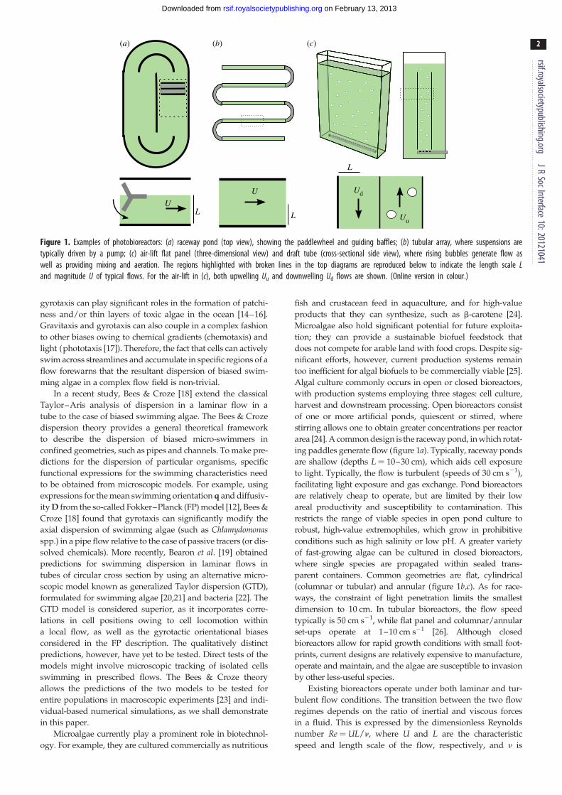
Figure 1. Examples of photobioreactors: (a) raceway pond (top view), showing the paddlewheel and guiding baffles; (b) tubular array, where suspensions aretypically driven by a pump; (c) air-lift flat panel (three-dimensional view) and draft tube (cross-sectional side view), where rising bubbles generate flow aswell as providing mixing and aeration. The regions highlighted with broken lines in the top diagrams are reproduced below to indicate the length scale Land magnitude U of typical flows. For the air-lift in (c), both upwelling Uu and downwelling Ud flows are shown. (Online version in colour.)

rsif.royalsocietypublishing.orgJR

SocInterface10:20121041

2

on February 13, 2013rsif.royalsocietypublishing.orgDownloaded from

gyrotaxis can play significant roles in the formation of patchi-

ness and/or thin layers of toxic algae in the ocean [14–16].

Gravitaxis and gyrotaxis can also couple in a complex fashion

to other biases owing to chemical gradients (chemotaxis) and

light (phototaxis [17]). Therefore, the fact that cells can actively

swim across streamlines and accumulate in specific regions of a

flow forewarns that the resultant dispersion of biased swim-

ming algae in a complex flow field is non-trivial.

In a recent study, Bees & Croze [18] extend the classical

Taylor–Aris analysis of dispersion in a laminar flow in a

tube to the case of biased swimming algae. The Bees & Croze

dispersion theory provides a general theoretical framework

to describe the dispersion of biased micro-swimmers in

confined geometries, such as pipes and channels. To make pre-

dictions for the dispersion of particular organisms, specific

functional expressions for the swimming characteristics need

to be obtained from microscopic models. For example, using

expressions for the mean swimming orientation q and diffusiv-

ity D from the so-called Fokker–Planck (FP) model [12], Bees &

Croze [18] found that gyrotaxis can significantly modify the

axial dispersion of swimming algae (such as Chlamydomonasspp.) in a pipe flow relative to the case of passive tracers (or dis-

solved chemicals). More recently, Bearon et al. [19] obtained

predictions for swimming dispersion in laminar flows in

tubes of circular cross section by using an alternative micro-

scopic model known as generalized Taylor dispersion (GTD),

formulated for swimming algae [20,21] and bacteria [22]. The

GTD model is considered superior, as it incorporates corre-

lations in cell positions owing to cell locomotion within

a local flow, as well as the gyrotactic orientational biases

considered in the FP description. The qualitatively distinct

predictions, however, have yet to be tested. Direct tests of the

models might involve microscopic tracking of isolated cells

swimming in prescribed flows. The Bees & Croze theory

allows the predictions of the two models to be tested for

entire populations in macroscopic experiments [23] and indi-

vidual-based numerical simulations, as we shall demonstrate

in this paper.

Microalgae currently play a prominent role in biotechnol-

ogy. For example, they are cultured commercially as nutritious

fish and crustacean feed in aquaculture, and for high-value

products that they can synthesize, such as b-carotene [24].

Microalgae also hold significant potential for future exploita-

tion; they can provide a sustainable biofuel feedstock that

does not compete for arable land with food crops. Despite sig-

nificant efforts, however, current production systems remain

too inefficient for algal biofuels to be commercially viable [25].

Algal culture commonly occurs in open or closed bioreactors,

with production systems employing three stages: cell culture,

harvest and downstream processing. Open bioreactors consist

of one or more artificial ponds, quiescent or stirred, where

stirring allows one to obtain greater concentrations per reactor

area [24]. A common design is the raceway pond, in which rotat-

ing paddles generate flow (figure 1a). Typically, raceway ponds

are shallow (depths L ¼ 10–30 cm), which aids cell exposure

to light. Typically, the flow is turbulent (speeds of 30 cm s21),

facilitating light exposure and gas exchange. Pond bioreactors

are relatively cheap to operate, but are limited by their low

areal productivity and susceptibility to contamination. This

restricts the range of viable species in open pond culture to

robust, high-value extremophiles, which grow in prohibitive

conditions such as high salinity or low pH. A greater variety

of fast-growing algae can be cultured in closed bioreactors,

where single species are propagated within sealed trans-

parent containers. Common geometries are flat, cylindrical

(columnar or tubular) and annular (figure 1b,c). As for race-

ways, the constraint of light penetration limits the smallest

dimension to 10 cm. In tubular bioreactors, the flow speed

typically is 50 cm s21, while flat panel and columnar/annular

set-ups operate at 1–10 cm s21 [26]. Although closed

bioreactors allow for rapid growth conditions with small foot-

prints, current designs are relatively expensive to manufacture,

operate and maintain, and the algae are susceptible to invasion

by other less-useful species.

Existing bioreactors operate under both laminar and tur-

bulent flow conditions. The transition between the two flow

regimes depends on the ratio of inertial and viscous forces

in a fluid. This is expressed by the dimensionless Reynolds

number Re ¼ UL/n, where U and L are the characteristic

speed and length scale of the flow, respectively, and n is

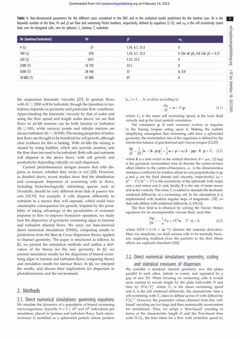
Table 1. Non-dimensional parameters for the different cases considered in the DNS and in the analytical model predictions for the laminar case. Re is theReynolds number of the flow, Pe and b are flow and swimming Peclet numbers, respectively, defined by equations (2.13), and a0 is the cell eccentricity (morethan zero for elongated cells, zero for spheres). L, laminar; T, turbulent.

Re (laminar/turbulent) Pe b a0

4 (L) 27 1.34, 6.7, 33.5 0

100 (L) 670 1.34, 6.7, 33.5 0 (for all b), 0.8 (for b ¼ 6.7)

250 (L) 1675 3.35, 33.5 0

2500 (T) 16 750 33.5 0

4200 (T) 28 140 55 0, 0.8

10 000 (T) 67 000 67 0

rsif.royalsocietypublishing.orgJR

SocInterface10:20121041

3

on February 13, 2013rsif.royalsocietypublishing.orgDownloaded from

the suspension kinematic viscosity [27]. In general, flows

with Re . 2000 will be turbulent, though the transition to tur-

bulence depends on geometry and particular flow conditions.

Approximating the kinematic viscosity by that of water and

using the flow speed and length scales above, we see that

flows in air-lift reactors can be both laminar or turbulent

(Re � 100), while raceway ponds and tubular reactors are

always turbulent (Re . 30 000). The mixing properties of turbu-

lent flows are thought to be beneficial for cell growth, although

clear evidence for this is lacking. With air-lifts the mixing is

caused by rising bubbles, which also provide aeration, and

the flow does not need to be turbulent. Both cells and nutrients

will disperse in the above flows, with cell growth and

productivity depending critically on such dispersion.

Current photobioreactor designs assume that cells dis-

perse as tracers, whether they swim or not [28]. However,

as detailed above, recent studies show that the distribution

and consequent dispersion of swimming cells in flows,

including biotechnologically interesting species such as

Dunaliella, should be very different from that of passive tra-

cers [18,19]. For example, if cells disperse differently to

nutrients in a reactor they will separate, which could have

catastrophic consequences for growth. Inspired by the possi-

bility of taking advantage of the peculiarities of swimmer

response to flow to improve bioreactor operation, we study

here the dispersion of gyrotactic swimming algae in laminar

and turbulent channel flows. We carry out time-resolved

direct numerical simulations (DNSs), comparing results to

predictions from the Bees & Croze dispersion theory applied

to channel geometry. The paper is structured as follows. In

§2, we present the simulation methods and outline a deri-

vation of the theory for the new geometry. In §3, we

present simulation results for the dispersion of biased swim-

ming algae in laminar and turbulent flows, comparing theory

and simulation results for laminar flows. In §4, we interpret

the results, and discuss their implications for dispersion in

photobioreactors and the environment.

2. Methods2.1. Direct numerical simulations: governing equationsWe simulate the dynamics of a population of biased swimming

micro-organisms, typically N ¼ 2 � 105 and 106 individuals per

simulation, placed in laminar and turbulent flows. Each micro-

swimmer is modelled as a spheroidal particle whose position

xi, i ¼ 1 . . . N, evolves according to

dxi

dt¼ uþ Vsp; ð2:1Þ

where Vs is the mean cell swimming speed, u the local fluid

velocity and p the local particle orientation.

The orientation p of each swimmer evolves in response

to the biasing torques acting upon it. Making the realistic

simplifying assumption that swimming cells have a spheroidal

geometry, the reorientation rate of the organisms is defined by the

inertia-free balance of gravitational and viscous torques [12,29]

dp

dt¼ 1

2B

hk� ðk � pÞp

iþ 1

2v� pþ a0ðI� ppÞ � E � pþ Gr; ð2:2Þ

where k is a unit vector in the vertical direction; B ¼ ma?/(2 hrg)

is the gyrotactic reorientation time (h denotes the centre-of-mass

offset relative to the centre-of-buoyancy, a? is the dimensionless

resistance coefficient for rotation about an axis perpendicular to p,

r and m are the fluid density and viscosity, respectively); a0 ¼

(a2 2 b2)/(a2 þ b2) is the eccentricity of the spheroids with major

axis a and minor axis b; and, finally, E is the rate of strain tensor

and v the vorticity. The noise Gr is added to simulate the stochastic

rotational diffusivity of a swimming cell. In the simulations it is

implemented with random angular steps of magnitudeffiffiffiffiffiffiffi2dr

p; so

that cells diffuse with rotational diffusivity dr [30,31].

The flow field u is obtained by solving the Navier–Stokes

equations for an incompressible viscous fluid, such that

Du

Dt¼ � 1

rrpþ nr2u; r � u ¼ 0; ð2:3Þ

where D/Dt ; @/@t þ (u .r) denotes the material derivative.

Here, for simplicity, we shall assume cells to be neutrally buoy-

ant, neglecting feedback from the particles to the flow (these

effects are explored elsewhere [18]).

2.2. Direct numerical simulations: geometry, scalingand statistical measures of dispersion

We consider a standard channel geometry: two flat plates

parallel to each other, infinite in extent, and separated by a

gap of size 2H. When focusing on swimming cells it would

seem natural to rescale length by the plate half-width H and

time by H2dr=V2s ; where Vs is the mean swimming speed

and dr is the cell rotational diffusivity, the characteristic time a

cell swimming with Vs takes to diffuse across H with diffusivity

V2s d�1

r : However, the parameter values obtained from this ‘cell-

based’ rescaling are too large and thus numerically inconvenient

for simulations. Thus, we adopt a ‘flow-based’ rescaling in

terms of the characteristic length H and the flow-based time

scale H/Uc, the time taken for a flow with centreline speed Uc

rsif.royalsocietypublishing.orgJR

SocInterface10:20121041

4

on February 13, 2013rsif.royalsocietypublishing.orgDownloaded from

to advect a cell by H. In terms of this rescaling, the dimensionless

equations of motion for a biased swimming cell are

dx�idt�¼ u� þ vsp; ð2:4Þ

dp

dt�¼ h�1[k� ðk � pÞp]þ 1

2w� � pþ a0ðI� ppÞ � E� � pþ G �r

ð2:5Þ

andDu�

Dt�¼ �r�pþ Re�1r�2u�; r � u� ¼ 0; ð2:6Þ

where starred quantities denote dimensionless variables.

In particular, we define the dimensionless swimming speed

vs ¼ Vs/Uc, the gyrotactic parameter h ¼ 2BUc/H and the

Reynolds number

Re ¼ UcHn

; ð2:7Þ

where Uc is the centreline speed, H is the channel half-width

and n the fluid’s kinematic viscosity. Non-dimensionalizing

the noise Gr also defines the dimensionless rotational

diffusivity d�r ¼ drH=Uc:

We adopt a Cartesian coordinate system where the mean

flow in the x (streamwise) direction varies with the wall-

normal coordinate y, and is independent of z(spanwise direction). We integrate equations (2.4)–(2.6) numeri-

cally (see the electronic supplementary material) to find

x�i ðt�Þ ¼ ½x�i ðt�Þ; y�i ðt�Þ; z�i ðt�Þ�: Enumerating the number of cells

N(x) at a given position x in a bin of fixed volume DV, we

obtain the cell concentration c(x) ¼ N(x)/DV. From the cell coor-

dinates we can further define statistical measures of the cell

dispersion in a flow: the adimensional drift L�0 with respect to

the mean flow U ¼ (2/3)Uc; the effective streamwise diffusivity

D�e; and the skewness of the cell distribution, g. These measures

of dispersion are given by

L�0ðt�Þ ;dm�1dt�� 2

3; D�eðt�Þ ;

1

2

d

dt�Varðx�Þ

and gðt�Þ ;m�3 � 3m�1m�2 þ 2m�31

Varðx�Þ3=2;

9>>=>>; ð2:8Þ

where m�p ¼ ð1=NÞP

iðx�i Þp ( p ¼ 1,2,3) are the distribution

moments and Varðx�Þ ¼ m�2 �m�21 is the variance of the cell distri-

bution. The statistical measures can be transformed from the flow-

based scaling with characteristic time scale H/Uc to the cell-based

scaling with time scale H2dr=V2s by the transformations

t� ! t ;t�

Pe; L�0 ! L0 ; L�0 Pe

and D�e ! De ; D�e Pe;

9=; ð2:9Þ

where Pe is the cell Peclet number defined with respect to the cen-

treline speed (see equation (2.13)). Note that the skewness g does

not depend on the scaling used. We shall present results in terms

of the cell-based scaling and compare their limit at long times

with analytical predictions.

2.3. Analytical theory: dispersion in laminar flows atlong times

Here, we shall obtain analytical predictions for the dispersion of

algae swimming in laminar channel flow that will be compared

with the results from the simulations. The general Bees & Croze

[18] continuum dispersion theory for biased swimmers will be

applied to the new channel geometry; it is valid in the long-

time limit (t�H2dr=V2s ). The derivation for channel flow is simi-

lar to the pipe flow example in Bees & Croze, so we provide an

outline here. Those readers who are less mathematically inclined

may skip the derivation of the results in this section.

We shall begin with the continuity equation for the cell

number density n:

@n@t¼ �r � ½nðuþVcÞ �D � rn�: ð2:10Þ

The flow velocity u is the solution of the Navier–Stokes equation

(2.3). We adopt the same coordinate system described above for

the DNS. For laminar flows such that the flow downstream is

only a function of the wall-normal coordinate y, the flow velocity

can be expressed as

uðyÞ ¼ uðyÞex ¼ U½1þ xðyÞ�ex; ð2:11Þ

where U is the mean flow speed and x(y) describes the variation

in the streamwise direction about this mean. It is convenient

to translate to a reference frame travelling with the mean

flow, and non-dimensionalize length scales by H and time

scales by the time to diffuse across the channel H2dr=V2s : Thus,

x ¼ ðx�UtÞ=H; y ¼ y=H; z ¼ z=H and t ¼ V2s t=ðH2drÞ; where

variables with hats denote dimensionless variables.

We assume unidirectional coupling of the cell dynamics to

the flow (for bidirectional coupling owing to non-neutrally buoy-

ant cells, see [18]): cells are biased by shear in the flow, so that the

cell swimming velocity Vc ¼ Vsq, where q is the mean swimming

direction, and diffusivity tensor D are functions of local flow

gradients. Here, we consider analytical predictions for spheri-

cal cells (a0 ¼ 0), so cell orientation is only a function of

vorticity, v ¼ r� u ¼ �x 0ez:

Consider planar Poiseuille flow, x ¼ (1 2 3y2)/2 and

U ¼ (2/3)Uc [32], where Uc is the centreline (maximum) flow

speed. Equation (2.10) becomes

@n@t¼ r � ðD � rnÞ � 2

3Pexnx � br � ðnqÞ; ð2:12Þ

with

Pe ¼ UcHdr

V2s

and b ¼ Hdr

Vs; ð2:13Þ

where hats have been dropped for clarity. Pe is a Peclet number,

the dimensionless ratio of the rates of transport by the flow and

swimming diffusion, and b is the ratio of channel half-width to

the length a cell swims before reorienting significantly. Alterna-

tively, we can rewrite b ¼ HV2s dr=V2

s and interpret it as a

‘swimming’ Peclet number, the ratio of the rates of transport

by swimming and diffusion. No-flow and no-flux boundary con-

ditions will be applied to (2.12), such that

u ¼ 0 and n � ðD � rn� bqnÞ ¼ 0 on S; ð2:14Þ

where n is the unit vector normal to the channel boundary S.

As the flow is translationally invariant along x, the mean

swimming direction and diffusivity tensor are independent

of x: D ¼ D(y), q ¼ q(y). This permits a treatment of

dispersion using moments in a similar vein to that of Aris

[7]. The pth moment with respect to the axial direction is

defined as

cpðy; tÞ ¼ðþ1

�1

xpnðx; y; tÞdx; ð2:15Þ

provided xpn(x,y,t)! 0 as x! + 1. We denote cross-sectional

averages by overbars. The cross-sectionally averaged axial

moment is thus

mpðtÞ ¼ �cp ¼1

2

ð1

�1

cpðy; tÞdy: ð2:16Þ

In Cartesian coordinates, equation (2.12) becomes

nt ¼ ðDyyny � bqynþDxynxÞy þDxynxy

� ð23Pexþ bqxÞnx þDxxnxx: ð2:17Þ

0.2

0.4

0.6

u / U

c

0.8

–0.5 0 0.5y

1.0

0–1.0 1.0

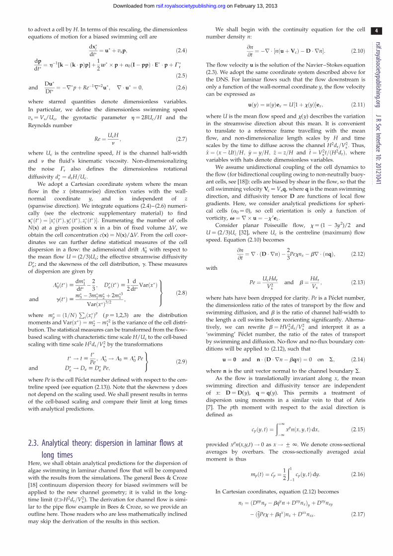
Figure 2. Flow profiles for the dimensionless flow speed as a function of yfor the laminar (black solid line) cases (self-similar for all Re) and time-averaged flow profiles for the turbulent cases (Re, Pe) ¼ (2500, 16 750),(4200, 28 140) and (10 000, 67 000), as shown by the dashed line, dottedline (blue) and grey (red) solid line, respectively. (Online version in colour.)

rsif.royalsocietypublishing.orgJR

SocInterface10:20121041

5

on February 13, 2013rsif.royalsocietypublishing.orgDownloaded from

Multiplying by xp and integrating over the length of an infi-

nite channel, we obtain the moment evolution equation

c p;t ¼ ðDyyc p;y � bqycp � pDxyc p�1Þy � pDxyc p�1;y

þ pð23Pexþ bqxÞc p�1 þ pð p� 1ÞDxxc p�2: ð2:18Þ

Averaging over the cross section and applying the no-flux

boundary conditions (2.14) yields

m p;t ¼ pð p� 1ÞDxxc p�2 � pDxyc p�1;y

þ p½23Pexþ bqx�c p�1 ð2:19Þ

from which we calculate measures of cell dispersion. The drift

above the mean flow, L0 ; limt!1ðd=dtÞm1ðtÞ; is given by

L0 ¼ �DxyY000 þ ½23Pexþ bqx�Y0

0; ð2:20Þ

where

Y00ðyÞ ¼ exp b

ðy

0

qyðsÞDyyðsÞds

� �exp b

ðy

0

qyðsÞDyyðsÞds

� �( )�1

ð2:21Þ

is the zeroth axial moment (normalized concentration profile).

Similarly, the effective diffusivity, De ; limt!1ð1=2Þðd=dtÞ[m2ðtÞ �m2

1ðtÞ�; is given by

De ¼ �Dxyg0 þ ½23Pexþ bqx � L0�gþDxxY00; ð2:22Þ

where gðyÞ ¼ Y00

Ð y0 ½ðDxyðsÞ=DyyðsÞÞ � ðL 0ðsÞ � L0 ~m0ðsÞÞ=DyyðsÞ

Y00ðsÞ�ds, with ~L0ðyÞ ¼

Ð y0 ½�DxyY0

0 þ ½23Pexþ bqx�Y00 ds and

~m0ðyÞ ¼Ð y

0 Y00 ds. The weighting function Y0

0ðyÞ controls the

drift and g(y) (related to the first axial moment) controls the

value of the diffusivity.

To make predictions from (2.20) and (2.22), we require

expressions for D and q from microscopic models of the statisti-

cal response of cells to flow. Two main models have been

proposed for biased swimming algae: the FP model [33,34] and

GTD [19–21]. For spherical cells, each model predicts how

non-dimensional swimming direction q and diffusivity D

depend on two non-dimensional quantities: s(y) ¼ 2 x‘(y)U/

(2drH ) ¼ 2 x’(y)(1/3)(Pe/b2), the ratio of reorientation time by

rotational diffusion to that by shear (vorticity), and l ¼ 1/

(2drB), the ratio between the time of reorientation by rotational

diffusion ð1=2Þd�1r and the gyrotactic reorientation time B. The

functional forms for the transport parameters q(s) and Dm(s),

where subscripts m ¼ F and G denote the FP and GTD models,

respectively, are given in appendix A [19]. In particular, the two

models differ qualitatively in their predictions for the diffusivity

as a function of the shear rate, and therefore they provide different

predictions for cell distribution and dispersion. The dispersion pre-

dictions (2.20) and (2.22) were evaluated numerically with MATLAB

(Mathworks, Natick, MA, USA) using q(s) and Dm(s) from the

two models (see electronic supplementary material).

2.4. Parameters, simulation time and flow profilesIn simulations and theoretical evaluations we used the following cell

parameters based on Chlamydomonas augustae: Vs ¼ 0.01 cm s21

(swimming speed), dr ¼ 0.067 s21 (cell rotational diffusivity), and

B ¼ 3.4 s (gyrotactic reorientation time) [18]. Furthermore, we

consider the flow of suspensions taken to have the same viscosity

as water, n ¼ 0.01 cm2 s21. The cell eccentricity a0 is also held

fixed. The analytical theory presented above assumes that cells are

spherical, a0 ¼ 0, but laminar and turbulent simulations have also

been performed for elongated cells with a0 ¼ 0.8. With these par-

ameters fixed, choosing the centreline speed Uc and channel width

H gives the non-dimensional flow-based parameters used in the

DNS: vs ¼ Vs/Uc (dimensionless swimming speed), h¼ 2BUc/H(gyrotactic parameter), d�r ¼ drH=Uc (dimensionless rotational

diffusivity) and Reynolds number Re ¼ UcH/n. For the test

run with passive tracers an additional noise term was added to

equation (2.4) to simulate the translational diffusivity Dt, non-

dimensionalized as D�t ¼ Dt=ðUcHÞ: These flow-based parameters

can be transformed into cell-based non-dimensional parameters

for comparison with analytical predictions. From the definitions

above and equation (2.13) it can be shown that Pe ¼ d�r=v2s (flow

Peclet number), b ¼ d�r=vs (swimming Peclet number) and

sðyÞ ¼ �ð1=3Þx 0ðyÞ=d�r (local dimensionless shear rate). Since

x0(y) ¼ 2 3y for plane Poiseuille flow, the maximum dimensionless

shear is given by jsmaxj ¼ 1=d�r ¼ hl;where we recall l ¼ 1/(2Bdr),

the non-dimensional bias parameter. Simulations are more readily

interpreted and compared with analytical theory in terms of these

parameters (shown in table 1).

The dimensionless flow profiles corresponding to the Rey-

nolds numbers used in this study are plotted in figure 2 for the

benefit of the reader. Laminar flows are self-similar, so the

non-dimensional flow has the same parabolic profile for all Re.

Time-averged turbulent flows have distinct profiles that

depend on the Reynolds number. Note that the number of

degrees of freedom in the turbulent flow simulations scales as

Re9 [27]. This makes large Re simulations computationally

expensive. For this reason, we do not investigate dispersion for

flows beyond Re ¼ 10 000.

3. Results3.1. Passive tracers: classical dispersionThe dispersion of passive tracers, such as molecular dyes or

non-motile cells, is generally well understood. In laminar chan-

nel flow passive tracers are transported on average at the mean

flow speed; there is no drift relative to mean flow: L0 ¼ 0. The

effective axial diffusivity De is given at long times by the

Taylor–Aris result De ¼ 1 þ (8/945)Pe2 [3,32]. As a bench-

mark test, we carried out DNS for passive tracers (solving

equation (2.4) with vs ¼ 0 and translational noise to simulate

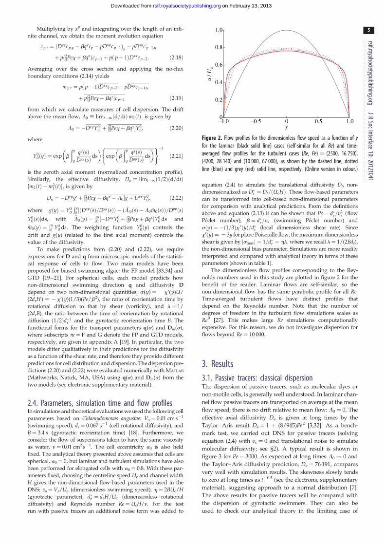
molecular diffusivity; see §2). A typical result is shown in

figure 3 for Pe ¼ 3000. As expected at long times L0! 0 and

the Taylor–Aris diffusivity prediction, De ¼ 76 191, compares

very well with simulation results. The skewness slowly tends

to zero at long times as t20.5 (see the electronic supplementary

material), suggesting approach to a normal distribution [7].

The above results for passive tracers will be compared with

the dispersion of gyrotactic swimmers. They can also be

used to check our analytical theory in the limiting case of

1 × 105

9 × 104

8 × 104

7 × 104

6 × 104

5 × 104

4 × 104

3 × 104

10–2

10–2 10–1 10 102

gL0

1

10–1 1 10 102

De

t

DNSTaylor–Aris

–0.6

–0.4

–0.2

0

0.2

t

Figure 3. Time dependence of the effective diffusivity, De, for passive tracersin a laminar flow with Pe ¼ 3000. For long times De ≃76191; the constantvalue predicted from the classical Taylor – Aris dispersion for passive tracers(see text). The inset shows the expected zero drift, L0, above the meanflow and the skewness, g, tending to zero at long times, suggesting anapproach to the expected normally distributed axial concentration profile[7]. (Online version in colour.)

–1.0 –0.5 0 0.5y

105

(a)

(b)

(c)

(d)

104

103c

102

10

105

104

103c

102

10

105

104

103c

102

10

105

104

103c

102

10

Pe = 27, b = 1.34b/Pe = 0.05

Pe = 1675, b = 33.5b/Pe = 0.02

Pe = 670, b = 6.7b/Pe = 0.01

Pe = 1675, b = 3.35b/Pe = 0.002

t = 3.7

t = 0.06t = 0.18t = 0.48t = 35.8

t = 7.4t = 2222

1.0

t = 0.75t = 1.2t = 89.6

t = 0.15

t = 7.16t = 18.5t = 35.8

t = 0.06

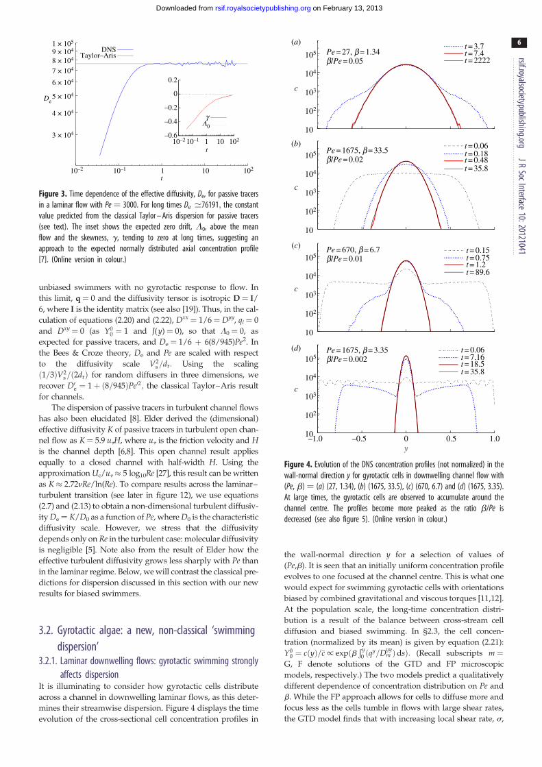
Figure 4. Evolution of the DNS concentration profiles (not normalized) in thewall-normal direction y for gyrotactic cells in downwelling channel flow with(Pe, b) ¼ (a) (27, 1.34), (b) (1675, 33.5), (c) (670, 6.7) and (d) (1675, 3.35).At large times, the gyrotactic cells are observed to accumulate around thechannel centre. The profiles become more peaked as the ratio b/Pe isdecreased (see also figure 5). (Online version in colour.)

rsif.royalsocietypublishing.orgJR

SocInterface10:20121041

6

on February 13, 2013rsif.royalsocietypublishing.orgDownloaded from

unbiased swimmers with no gyrotactic response to flow. In

this limit, q ¼ 0 and the diffusivity tensor is isotropic D ¼ I/

6, where I is the identity matrix (see also [19]). Thus, in the cal-

culation of equations (2.20) and (2.22), Dxx¼ 1/6 ¼ Dyy, qi ¼ 0

and Dxy¼ 0 (as Y00 ¼ 1 and J(y) ¼ 0), so that L0 ¼ 0, as

expected for passive tracers, and De ¼ 1/6 þ 6(8/945)Pe2. In

the Bees & Croze theory, De and Pe are scaled with respect

to the diffusivity scale V2s=dr: Using the scaling

ð1=3ÞV2s=ð2drÞ for random diffusers in three dimensions, we

recover D0e ¼ 1þ ð8=945ÞPe02; the classical Taylor–Aris result

for channels.

The dispersion of passive tracers in turbulent channel flows

has also been elucidated [8]. Elder derived the (dimensional)

effective diffusivity K of passive tracers in turbulent open chan-

nel flow as K ¼ 5.9 utH, where ut is the friction velocity and His the channel depth [6,8]. This open channel result applies

equally to a closed channel with half-width H. Using the

approximation Uc/ut � 5 log10Re [27], this result can be written

as K � 2.72nRe/ln(Re). To compare results across the laminar–

turbulent transition (see later in figure 12), we use equations

(2.7) and (2.13) to obtain a non-dimensional turbulent diffusiv-

ity De ¼ K/D0 as a function of Pe, where D0 is the characteristic

diffusivity scale. However, we stress that the diffusivity

depends only on Re in the turbulent case: molecular diffusivity

is negligible [5]. Note also from the result of Elder how the

effective turbulent diffusivity grows less sharply with Pe than

in the laminar regime. Below, we will contrast the classical pre-

dictions for dispersion discussed in this section with our new

results for biased swimmers.

3.2. Gyrotactic algae: a new, non-classical ‘swimmingdispersion’

3.2.1. Laminar downwelling flows: gyrotactic swimming stronglyaffects dispersion

It is illuminating to consider how gyrotactic cells distribute

across a channel in downwelling laminar flows, as this deter-

mines their streamwise dispersion. Figure 4 displays the time

evolution of the cross-sectional cell concentration profiles in

the wall-normal direction y for a selection of values of

(Pe,b). It is seen that an initially uniform concentration profile

evolves to one focused at the channel centre. This is what one

would expect for swimming gyrotactic cells with orientations

biased by combined gravitational and viscous torques [11,12].

At the population scale, the long-time concentration distri-

bution is a result of the balance between cross-stream cell

diffusion and biased swimming. In §2.3, the cell concen-

tration (normalized by its mean) is given by equation (2.21):

Y00 ¼ cðyÞ=�c/ expðb

Ð y0 ðqy=Dyy

m ÞdsÞ: (Recall subscripts m ¼G, F denote solutions of the GTD and FP microscopic

models, respectively.) The two models predict a qualitatively

different dependence of concentration distribution on Pe and

b. While the FP approach allows for cells to diffuse more and

focus less as the cells tumble in flows with large shear rates,

the GTD model finds that with increasing local shear rate, s,

102

10

1

c / − c

10–1

10–2

10–30 0.1 0.2 0.3 0.4 0.5 0.6 0.7 0.8

y

GTD b/Pe = 0.002FP b/Pe = 0.002

GTD b/Pe = 0.01FP b/Pe = 0.01

GTD/FP b/Pe = 0.02GTD/FP b/Pe = 0.25

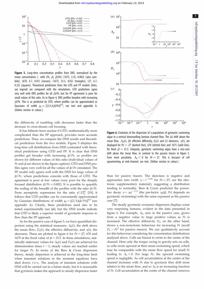
Figure 5. Long-time concentration profiles from DNS, normalized by themean concentration �c; with (Pe, b, b/Pe): (1675, 3.35, 0.002) ( plus sym-bols), (670, 6.7, 0.01) (crosses), (1675, 33.5, 0.02) (triangles), (27, 6.7,0.25) (squares). Theoretical predictions from the GTD and FP models (lines,see legend) are compared with the simulations. GTD predictions agreevery well with DNS profiles for all b/Pe, but for FP agreement is poor forsmall values of this ratio. As in figure 4, DNS profiles broaden with increasingb/Pe. This is as predicted by GTD, where profiles can be approximated asGaussians of width y0 ¼ [(2/l)(b/Pe)]0.5; see text and appendix A.(Online version in colour.)

t

103

102

10

103

De

104

102

10

10–3 10–2 10–1 10 102 103 1041

t10–1 10 102 103 1041

0

–0.2

–0.4

–0.6

–0.8

–1.0

–1.2

–6

–5

–4

–3

–2

L0 L0

g

(a)

(b)

(c)

Figure 6. Evolution of the dispersion of a population of gyrotactic swimmingalgae in a vertical downwelling laminar channel flow. The (a) drift above themean flow, L0(t), (b) effective diffusivity, De(t) and (c) skewness, g(t), aredisplayed for Pe ¼ 27 (dashed line), 670 (dotted line) and 1675 (solid line),for fixed b ¼ 33.5. Uniquely, gyrotactic swimming algae have a non-zerodrift above the mean flow, in contrast to the passive tracers in figure 3.Even more peculiarly, L0 , 0 for Pe ¼ 27. This is because of cellupswimming at mid-channel; see text. (Online version in colour.)

rsif.royalsocietypublishing.orgJR

SocInterface10:20121041

7

on February 13, 2013rsif.royalsocietypublishing.orgDownloaded from

the diffusivity of tumbling cells decreases faster than the

decrease in cross-stream cell focusing.

It has hitherto been unclear if GTD, mathematically more

complicated than the FP approach, provides more accurate

predictions. Thus, we compare the DNS results and theoreti-

cal predictions from the two models. Figure 5 displays the

long-time cell distributions from DNS contrasted with theor-

etical predictions using GTD and FP. It is clear that DNS

profiles get broader with increasing b/Pe, so profiles are

shown for different values of this ratio (individual values of

Pe and b are shown in the figure caption). GTD and DNS pro-

files agree very well for all the values of b/Pe simulated. The

FP model only agrees well with the DNS for large values of

b/Pe, where predictions coincide with those of GTD. The

agreement is poor at low values (very poor for the sharply

focused distribution b/Pe ¼ 0.002). It is possible to quantify

the scaling of the breadth of the profiles with the ratio b/Pe.From asymptotic expressions for the ratio qy=Dyy

G [19], it

follows that GTD profiles can be conveniently approximated

by Gaussian distributions of width y0 ¼ [(2/l)(b/Pe)]0.5 (see

appendix A). Clearly, these predictions need also to be

tested experimentally (see §4), but the DNS results indicate

that GTD is likely a superior model of gyrotactic response to

flow than the FP approach.

As for the passive case of figure 3, we have quantified dis-

persion using the statistical measures: L0(t), the drift above

the mean flow; De(t), the effective diffusivity; and g(t), the

skewness. These are plotted in figure 6 for Pe ¼ 27, 670 and

1675 at the fixed value of b ¼ 33.5. In these simulations, stat-

istically stationary values for L0(t) and De(t) are achieved for

dimensionless times t � 1; steady values are reached earlier

for larger Pe. In terms of the Bees & Croze dispersion

theory, steady dispersion is achieved in the long-time limit

when transient solutions to the moment equations have

died down: t�t1. The analysis of transient solutions with

DNS will be carried out in a future study, but it is reasonable

that gyrotaxis makes the approach to steady dispersion faster

than for passive tracers. The skewness is negative and

approaches zero (with g � t20.49 for Pe ¼ 27; see the elec-

tronic supplementary material), suggesting a distribution

tending to normality. Bees & Croze predicted the power-

law decay g ¼ g0t21/2 (the pre-factor g0(b, Pe) depends on

gyrotactic swimming) with the same exponent as the passive

case [7].

The steady gyrotactic swimmer dispersion displays some

very surprising features, evident in the data presented in

figure 6. For example, L0, zero in the passive case, grows

from a negative value to large positive values as Pe is

increased. The effective diffusivity De, on the other hand,

shows a non-monotonic behaviour for increasing Pe (recall

De � Pe2 for passive tracers). We can qualitatively account

for this behaviour considering the concentration distributions

analysed above. Cells are biased to swim to the centre of the

channel. Here only the torque owing to gravity acts on cells,

so cells swim upward at their mean swimming speed, which

may be comparable with the mean flow speed for small Peleading to L0 , 0. For large Pe, the upward swimming

speed is negligible. As cell accumulation at the centre of the

channel increases with Pe due to gyrotaxis they drift more

relative to the mean flow, and so L0 is an increasing function

of Pe. Cell accumulation at the centre of the channel removes

0

0.1

0.2

0.3c

c

0.4

0.5

0.6

–1.0 –0.5 0 0.5 1.0y

00.10.20.30.40.50.6

0.94 0.96 0.98 1.00y

Pe = 16750, b = 33.5, b/Pe = 0.002Pe = 28140, b = 55, b/Pe = 0.002Pe = 67000, b = 67, b/Pe = 0.001

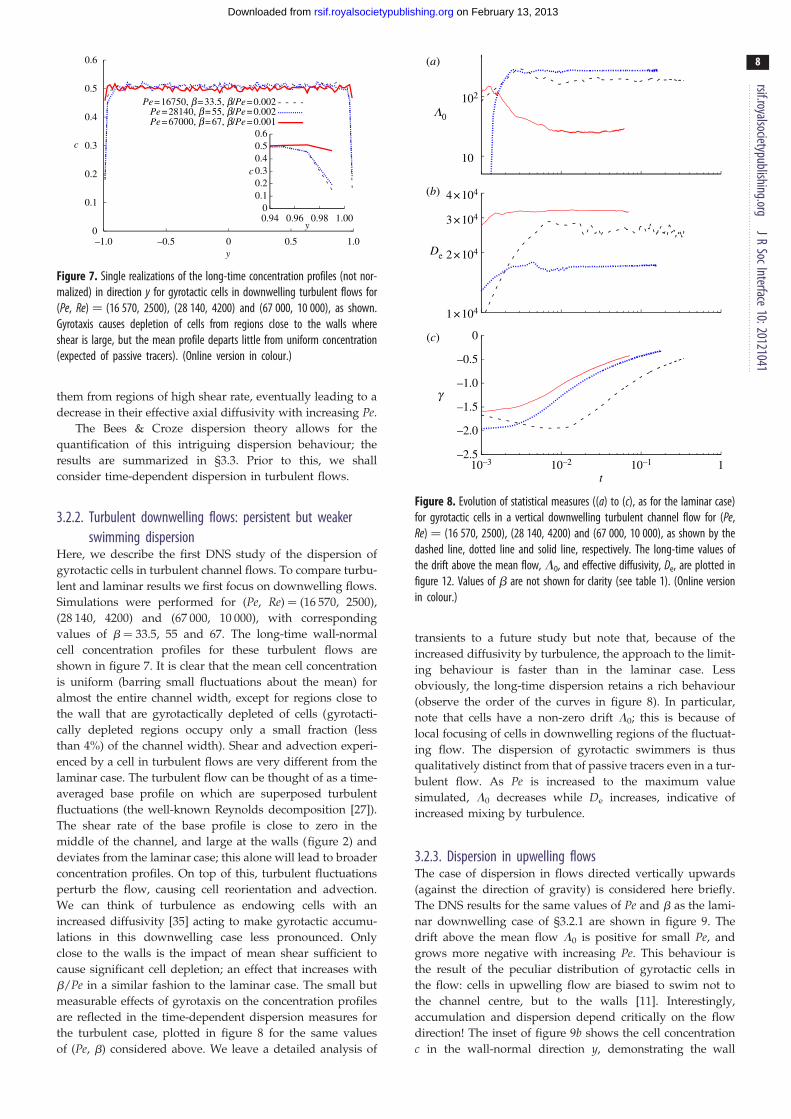
Figure 7. Single realizations of the long-time concentration profiles (not nor-malized) in direction y for gyrotactic cells in downwelling turbulent flows for(Pe, Re) ¼ (16 570, 2500), (28 140, 4200) and (67 000, 10 000), as shown.Gyrotaxis causes depletion of cells from regions close to the walls whereshear is large, but the mean profile departs little from uniform concentration(expected of passive tracers). (Online version in colour.)

t

De

L0

g

(a)

(b)

(c)

102

10

4 × 104

3 × 104

2 × 104

1 × 104

10–3 10–2 10–1 1

0

–0.5

–1.0

–1.5

–2.0

–2.5

rsif.royalsocietypublishing.orgJR

SocInterface10:20121041

8

on February 13, 2013rsif.royalsocietypublishing.orgDownloaded from

them from regions of high shear rate, eventually leading to a

decrease in their effective axial diffusivity with increasing Pe.

The Bees & Croze dispersion theory allows for the

quantification of this intriguing dispersion behaviour; the

results are summarized in §3.3. Prior to this, we shall

consider time-dependent dispersion in turbulent flows.

Figure 8. Evolution of statistical measures ((a) to (c), as for the laminar case)for gyrotactic cells in a vertical downwelling turbulent channel flow for (Pe,Re) ¼ (16 570, 2500), (28 140, 4200) and (67 000, 10 000), as shown by thedashed line, dotted line and solid line, respectively. The long-time values ofthe drift above the mean flow, L0, and effective diffusivity, De, are plotted infigure 12. Values of b are not shown for clarity (see table 1). (Online versionin colour.)

3.2.2. Turbulent downwelling flows: persistent but weakerswimming dispersion

Here, we describe the first DNS study of the dispersion of

gyrotactic cells in turbulent channel flows. To compare turbu-

lent and laminar results we first focus on downwelling flows.

Simulations were performed for (Pe, Re) ¼ (16 570, 2500),

(28 140, 4200) and (67 000, 10 000), with corresponding

values of b ¼ 33.5, 55 and 67. The long-time wall-normal

cell concentration profiles for these turbulent flows are

shown in figure 7. It is clear that the mean cell concentration

is uniform (barring small fluctuations about the mean) for

almost the entire channel width, except for regions close to

the wall that are gyrotactically depleted of cells (gyrotacti-

cally depleted regions occupy only a small fraction (less

than 4%) of the channel width). Shear and advection experi-

enced by a cell in turbulent flows are very different from the

laminar case. The turbulent flow can be thought of as a time-

averaged base profile on which are superposed turbulent

fluctuations (the well-known Reynolds decomposition [27]).

The shear rate of the base profile is close to zero in the

middle of the channel, and large at the walls (figure 2) and

deviates from the laminar case; this alone will lead to broader

concentration profiles. On top of this, turbulent fluctuations

perturb the flow, causing cell reorientation and advection.

We can think of turbulence as endowing cells with an

increased diffusivity [35] acting to make gyrotactic accumu-

lations in this downwelling case less pronounced. Only

close to the walls is the impact of mean shear sufficient to

cause significant cell depletion; an effect that increases with

b/Pe in a similar fashion to the laminar case. The small but

measurable effects of gyrotaxis on the concentration profiles

are reflected in the time-dependent dispersion measures for

the turbulent case, plotted in figure 8 for the same values

of (Pe, b) considered above. We leave a detailed analysis of

transients to a future study but note that, because of the

increased diffusivity by turbulence, the approach to the limit-

ing behaviour is faster than in the laminar case. Less

obviously, the long-time dispersion retains a rich behaviour

(observe the order of the curves in figure 8). In particular,

note that cells have a non-zero drift L0; this is because of

local focusing of cells in downwelling regions of the fluctuat-

ing flow. The dispersion of gyrotactic swimmers is thus

qualitatively distinct from that of passive tracers even in a tur-

bulent flow. As Pe is increased to the maximum value

simulated, L0 decreases while De increases, indicative of

increased mixing by turbulence.

3.2.3. Dispersion in upwelling flowsThe case of dispersion in flows directed vertically upwards

(against the direction of gravity) is considered here briefly.

The DNS results for the same values of Pe and b as the lami-

nar downwelling case of §3.2.1 are shown in figure 9. The

drift above the mean flow L0 is positive for small Pe, and

grows more negative with increasing Pe. This behaviour is

the result of the peculiar distribution of gyrotactic cells in

the flow: cells in upwelling flow are biased to swim not to

the channel centre, but to the walls [11]. Interestingly,

accumulation and dispersion depend critically on the flow

direction! The inset of figure 9b shows the cell concentration

c in the wall-normal direction y, demonstrating the wall

t

0 0.2 0.4 0.6 0.8 1.0y

De

–L0

L0

(a)

(b)

104

108

107

106

105

104

103

102

101

10

105

104

103c

102

101

103

102

10

10

10–1

10–2

10–3 10–2 10–1 10 102 103 1041

t10–1 10 102 103 1041

1

1

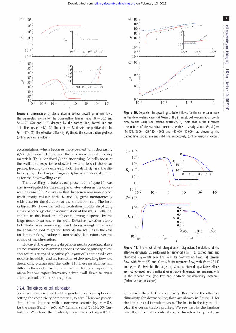
Figure 9. Dispersion of gyrotactic algae in vertical upwelling laminar flows.The parameters are as for the downwelling laminar case (b ¼ 33.5 andPe ¼ 27, 670 and 1675 denoted by the dashed line, dotted line andsolid line, respectively). (a) The drift 2L0 (inset: the positive drift forPe ¼ 27). (b) The effective diffusivity De (inset: the concentration profiles).(Online version in colour.)

t

0.950 0.975 1.000y

L0

105

104

103

107

106

105

104

10–3 10–2 10–1 1

102 102

10

10–1

10–2

10–3

1

10

10–1

10–2

1c

De

(a)

(b)

Figure 10. Dispersion in upwelling turbulent flows for the same parametersas the downwelling case. (a) Mean drift L0 (inset: cell concentration profileclose to the wall). (b) Effective diffusivity De. Note that in the turbulentcase neither of the statistical measures reaches a steady value. (Pe, Re) ¼(16 570, 2500), (28 140, 4200) and (67 000, 10 000), as shown by thedashed line, dotted line and solid line, respectively. (Online version in colour.)

10–1

1

10

102

103

10–3 10–2 10–1 1

De

De

t

00.10.20.30.40.50.6

0.950 0.975 1.000

c

y

10–1

1

10

102

103

104

105(a)

(b)10–2 10–1 1 10 102 103

10–2

10–1

1

10

0 0.1 0.2 0.3c/

c –

y

Figure 11. The effect of cell elongation on dispersion. Simulations of theeffective diffusivity De performed for spherical (a0 ¼ 0, dashed line) andelongated (a0 ¼ 0.8, solid line) cells for downwelling flows. (a) Laminarflow, with Pe ¼ 670 and b ¼ 6.7; (b) turbulent flow, with Pe ¼ 28 140and b ¼ 55. Even for the large a0 value considered, qualitative effectsare not observed and significant quantitative differences are apparent onlyin the laminar case (see text and electronic supplementary material).(Online version in colour.)

rsif.royalsocietypublishing.orgJR

SocInterface10:20121041

9

on February 13, 2013rsif.royalsocietypublishing.orgDownloaded from

accumulation, which becomes more peaked with decreasing

b/Pe (for more details, see the electronic supplementary

material). Thus, for fixed b and increasing Pe, cells focus at

the walls and experience slower flow and less of the shear

profile, leading to a decrease in both the drift, L0, and the dif-

fusivity, De. The change of sign in L0 has a similar explanation

as for the downwelling case.

The upwelling turbulent case, presented in figure 10, was

also investigated for the same parameter values as the down-

welling case of §3.2.2. We see that dispersion measures do not

reach steady values: both L0 and De grow monotonically

with time for the duration of the simulation run. The inset

in figure 10a shows the cell concentration profiles displaying

a thin band of gyrotactic accumulation at the walls. Cells that

end up in this band are subject to strong dispersal by the

large mean shear rate at the wall. Diffusion, whether owing

to turbulence or swimming, is not strong enough to balance

the shear-induced migration towards the wall, as is the case

for laminar flow, leading to non-steady dispersion over the

course of the simulations.

However, the upwelling dispersion results presented above

are not realistic for swimming species that are negatively buoy-

ant; accumulations of negatively buoyant cells at the walls can

result in instability and the formation of downwelling flow and

descending plumes near the walls [11]. These instabilities will

differ in their extent in the laminar and turbulent upwelling

cases, but we expect buoyancy-driven wall flows to ensue

after accumulation in both regimes.

3.2.4. The effects of cell elongationSo far we have assumed that the gyrotactic cells are spherical,

setting the eccentricity parameter a0 to zero. Here, we present

simulations obtained with a non-zero eccentricity, a0¼ 0.8,

for the cases (Pe, b) ¼ (670, 6.7) (laminar) and (28 140, 55) (tur-

bulent). We chose the relatively large value of a0 ¼ 0.8 to

emphasize the effect of eccentricity. Results for the effective

diffusivity for downwelling flow are shown in figure 11 for

the laminar and turbulent cases. The insets in the figure dis-

play the concentration profiles. We see that in the laminar

case the effect of eccentricity is to broaden the profile, as

rsif.royalsocietypublishing.org

10

on February 13, 2013rsif.royalsocietypublishing.orgDownloaded from

observed in Bearon et al. [36]. This broader distribution

results in an increased value of effective diffusivity (cells

sample more of the shear profile). In the turbulent case of

figure 11b, there is a much smaller broadening effect. The

effect of cell elongation on other statistical measures for the

parameters considered here is marginal (see the electronic

supplementary material). If realistic values of biflagellate

eccentricity (a0 ¼ 0–0.3 [13]) are used, predictions for the dis-

persion of biased swimmers are not very different from those

obtained here for spherical cells.

JRSocInterface

10:20121041

3.3. Long-time dispersion of gyrotactic cellsas a function of Pe (Re) across thelaminar – turbulent transition

Having analysed the full time dependence of gyrotactic cell

dispersion, we concentrate here on its long-time behaviour.

In this limit, laminar DNS results can be compared with pre-

dictions from analytical theory for drift L0 and diffusivity De

as functions of Pe (for given b). The theory requires as inputs

expressions for the mean swimming direction, q, and diffu-

sivity tensor, D, obtained from microscopic stochastic

models. We test two alternative microscopic models: FP

and GTD. The models predict qualitatively different func-

tional forms for the components of D as a function of the

dimensionless shear s. Correspondingly, predictions for

L0(Pe) and De(Pe) obtained with the two models also differ.

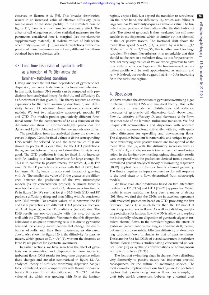
The predictions from the analytical theory are shown as

curves in figure 12a,b, for fixed values of b; the corresponding

DNS results for selected Pe and the same values of b are

shown as points. It is clear that, for the GTD predictions,

the agreement between theory and simulation for L0 is very

good. The GTD prediction is that, for fixed b, L0 increases

with Pe, tending to a linear behaviour for large enough Pe.

This is in contrast to passive tracers, for which L0 ¼ 0. For

small Pe the FP prediction coincides with that of GTD, but,

for larger Pe, L0 tends to a constant instead of growing

with Pe. The smaller the value of b, the greater is the differ-

ence between the predictions of the two microscopic

models (as for concentration profiles). A similar trend is

seen for the effective diffusivity De, shown as a function of

Pe in figure 12b. We see that for b ¼ 33.5, both GTD and FP

predict a diffusivity rising and then falling with Pe, consistent

with DNS results. For smaller values of b, however, the FP

and GTD predictions are different: GTD predicts a decrease

of De at large Pe, while FP predicts a (second) rise. The

DNS results are not compatible with this rise, but agree

well with the GTD prediction. We remark that this dispersion

behaviour is unique to swimming cells. It is due to gyrotactic

bias and the ensuing accumulations that change the distri-

bution of cells and thus their dispersion, as discussed

above. Also shown in figure 12b is the diffusivity for passive

tracers, which grows as De � Pe2 [4], without the decrease at

large Pe we predict for gyrotactic swimmers.

In earlier sections, we have seen how the effect of gyro-

taxis on accumulation and dispersion is more subtle in

turbulent flows. DNS results for long-time dispersion reflect

these changes and are also summarized in figure 12. An

analytical theory of turbulent swimming dispersion has yet

to be formulated, so we compare only with theory for passive

tracers. It is seen for all simulations with b ¼ 33.5 that the

value of L0, which was growing with Pe in the laminar

regime, drops a little just beyond the transition to turbulence.

On the other hand, the diffusivity De, which was falling at

large laminar Pe, suddenly acquires a sizeable value. The tur-

bulent shear profile and fluctuations alter the distribution of

cells. The effect of gyrotaxis is thus weakened but still mea-

surable in the dispersion, which is similar but not identical

to that of passive tracers. The fractional drift above the

mean flow speed U ¼ (2/3)Uc is given by d ; limt!1(1/

U )[dm1/dt 2 U ] ¼ (3/2)L0/Pe; this is rather small for large

turbulent Pe values. Nevertheless, it is remarkable that drift

should not be zero in a turbulent flow, as it is for passive tra-

cers. For very large values of Pe, we expect gyrotaxis to have

practically no effect on dispersion: the time-averaged concen-

tration profile will be well approximated as uniform and

L0 ¼ 0. Indeed, our results suggest that L0! 0 for increasing

Pe in the turbulent regime.

4. DiscussionWe have studied the dispersion of gyrotactic swimming algae

in channel flows by DNS and analytical theory. This is the

first study to evaluate cell distributions and statistical

measures of gyrotactic cell dispersion (drift above mean

flow L0, effective diffusivity De and skewness g) for flows

on either side of the laminar–turbulence transition. We find

unique cell accumulations and dispersion with non-zero

drift and a non-monotonic diffusivity with Pe, with quali-

tative differences for upwelling and downwelling flows.

The dispersion behaviour is remarkable and unique to gyro-

tactic swimming cells: passive tracers are transported at the

mean flow rate (L0 ¼ 0), the diffusivity increases with Pe(De � Pe2) [4], and dispersion is insensitive to channel orien-

tation. In the laminar downwelling regime, simulation results

were compared with the predictions derived from a recently

formulated general analytical theory of swimming dispersion

[18,19], applied here for the first time to channel geometry.

The theory requires as inputs expressions for cell response

to the local shear in a flow, determined from microscopic

models.

We have evaluated predictions based on two alternative

models: the FP [33,34] and GTD [19–21] approaches. Which

model is more realistic has long been a matter of debate

[20]. Here, we find that the DNSs are in excellent agreement

with analytical predictions based on GTD, providing the first

evidence that GTD is much better than the FP model at

describing swimmers in flows. As well as validating analyti-

cal predictions for laminar flow, the DNSs allow us to explore

the industrially relevant dispersion of gyrotactic algae in tur-

bulent channel flows. In the turbulent regime, the effects of

gyrtoaxis (accumulations resulting in non-zero drift) persist,

but are much more subtle. Effective diffusivity in downwel-

ling turbulent flows is similar to that of passive tracers.

These are the first full DNSs of biased swimmers in turbulent

channel flows; previous studies having concentrated on vor-

tical flow [37] or synthetic approximations of homogeneous

isotropic turbulence [31,35].

The fact that swimming algae in channel flows distribute

very differently to passive tracers has important practical

consequences for the culture of swimming species. The

most dramatic implications of our findings are for photobio-

reactors that operate using laminar flows. For example, in

draft tube air-lift bioreactors, bubbles up a central draft

1

10

102

103

10 102 103 104 105

1 10 102 103 104

Pe

Re

laminar turbulent

(a)

GTD, b = 1.34 FP, b = 1.34

GTD, b = 6.7 FP, b = 6.7

GTD/FP, b = 33.5

10–1

1

10

102

103

104

105

106

107

108

1 10 102 103 104 105

10–1 1 10 102 103 104

Pe

Re

laminar turbulent

(b)

GTD, b = 1.34FP, b = 1.34

GTD, b = 6.7FP, b = 6.7

GTD/FP, b = 33.5tracer (laminar)

tracer (turbulent)

L0

De

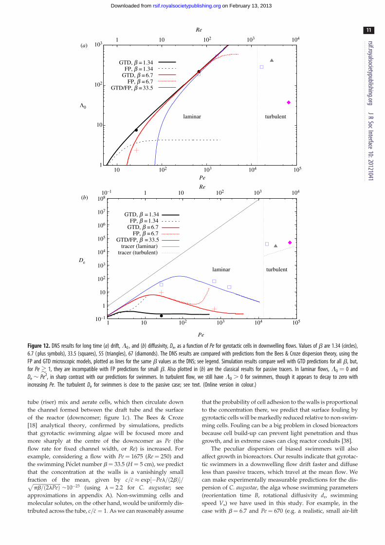
Figure 12. DNS results for long time (a) drift, L0 , and (b) diffusivity, De, as a function of Pe for gyrotactic cells in downwelling flows. Values of b are 1.34 (circles),6.7 ( plus symbols), 33.5 (squares), 55 (triangles), 67 (diamonds). The DNS results are compared with predictions from the Bees & Croze dispersion theory, using theFP and GTD microscopic models, plotted as lines for the same b values as the DNS; see legend. Simulation results compare well with GTD predictions for all b, but,for Pe � 1, they are incompatible with FP predictions for small b. Also plotted in (b) are the classical results for passive tracers. In laminar flows, L0 ¼ 0 andDe � Pe2, in sharp contrast with our predictions for swimmers. In turbulent flow, we still have L0 . 0 for swimmers, though it appears to decay to zero withincreasing Pe. The turbulent De for swimmers is close to the passive case; see text. (Online version in colour.)

rsif.royalsocietypublishing.orgJR

SocInterface10:20121041

11

on February 13, 2013rsif.royalsocietypublishing.orgDownloaded from

tube (riser) mix and aerate cells, which then circulate down

the channel formed between the draft tube and the surface

of the reactor (downcomer; figure 1c). The Bees & Croze

[18] analytical theory, confirmed by simulations, predicts

that gyrotactic swimming algae will be focused more and

more sharply at the centre of the downcomer as Pe (the

flow rate for fixed channel width, or Re) is increased. For

example, considering a flow with Pe ¼ 1675 (Re ¼ 250) and

the swimming Peclet number b ¼ 33.5 (H ¼ 5 cm), we predict

that the concentration at the walls is a vanishingly small

fraction of the mean, given by c=�c � exp½�Pel=ð2bÞ�=ffiffiffiffiffiffiffiffiffiffiffiffiffiffiffiffiffiffiffiffiffiffiffipb=ð2lPeÞ

p�10�23 (using l ¼ 2.2 for C. augustae; see

approximations in appendix A). Non-swimming cells and

molecular solutes, on the other hand, would be uniformly dis-

tributed across the tube, c=�c ¼ 1:As we can reasonably assume

that the probability of cell adhesion to the walls is proportional

to the concentration there, we predict that surface fouling by

gyrotactic cells will be markedly reduced relative to non-swim-

ming cells. Fouling can be a big problem in closed bioreactors

because cell build-up can prevent light penetration and thus

growth, and in extreme cases can clog reactor conduits [38].

The peculiar dispersion of biased swimmers will also

affect growth in bioreactors. Our results indicate that gyrotac-

tic swimmers in a downwelling flow drift faster and diffuse

less than passive tracers, which travel at the mean flow. We

can make experimentally measurable predictions for the dis-

persion of C. augustae, the alga whose swimming parameters

(reorientation time B, rotational diffusivity dr, swimming

speed Vs) we have used in this study. For example, in the

case with b ¼ 6.7 and Pe ¼ 670 (e.g. a realistic, small air-lift

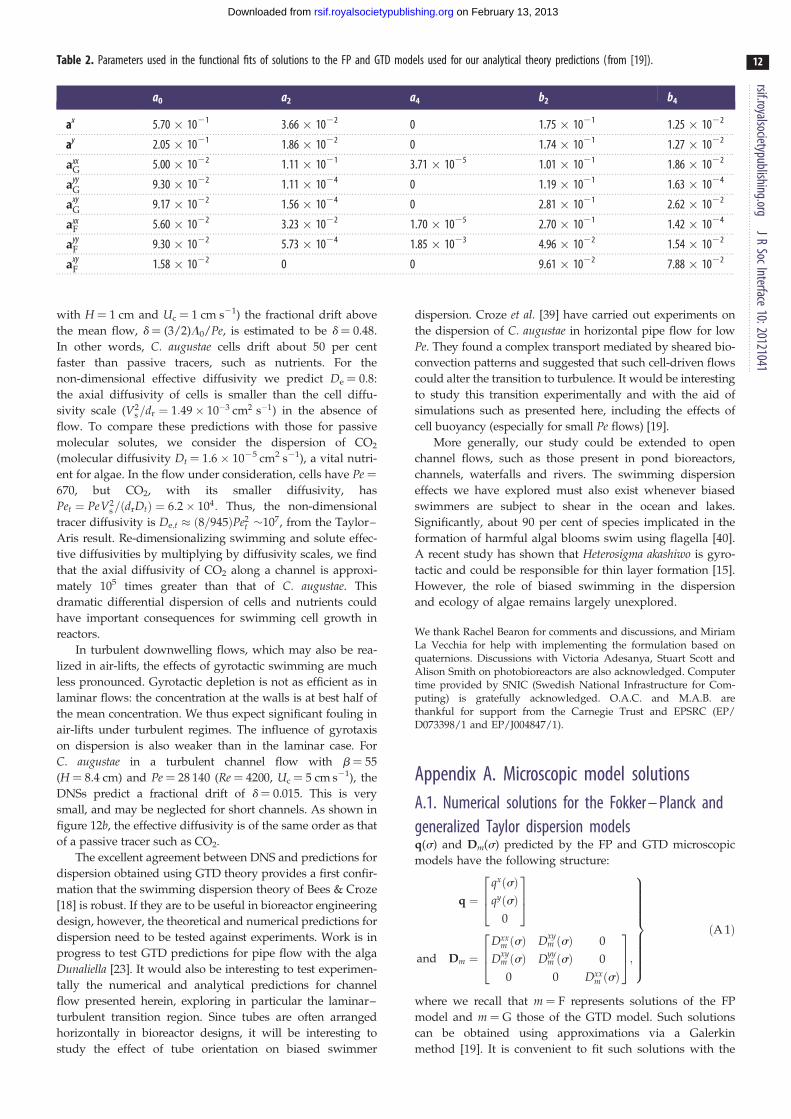
Table 2. Parameters used in the functional fits of solutions to the FP and GTD models used for our analytical theory predictions (from [19]).

a0 a2 a4 b2 b4

ax 5.70 � 1021 3.66 � 1022 0 1.75 � 1021 1.25 � 1022

ay 2.05 � 1021 1.86 � 1022 0 1.74 � 1021 1.27 � 1022

axxG 5.00 � 1022 1.11 � 1021 3.71 � 1025 1.01 � 1021 1.86 � 1022

ayyG 9.30 � 1022 1.11 � 1024 0 1.19 � 1021 1.63 � 1024

axyG 9.17 � 1022 1.56 � 1024 0 2.81 � 1021 2.62 � 1022

axxF 5.60 � 1022 3.23 � 1022 1.70 � 1025 2.70 � 1021 1.42 � 1024

ayyF 9.30 � 1022 5.73 � 1024 1.85 � 1023 4.96 � 1022 1.54 � 1022

axyF 1.58 � 1022 0 0 9.61 � 1022 7.88 � 1022

rsif.royalsocietypublishing.orgJR

SocInterface10:20121041

12

on February 13, 2013rsif.royalsocietypublishing.orgDownloaded from

with H ¼ 1 cm and Uc ¼ 1 cm s21) the fractional drift above

the mean flow, d ¼ (3/2)L0/Pe, is estimated to be d ¼ 0.48.

In other words, C. augustae cells drift about 50 per cent

faster than passive tracers, such as nutrients. For the

non-dimensional effective diffusivity we predict De ¼ 0.8:

the axial diffusivity of cells is smaller than the cell diffu-

sivity scale (V2s=dr ¼ 1:49� 10�3 cm2 s�1) in the absence of

flow. To compare these predictions with those for passive

molecular solutes, we consider the dispersion of CO2

(molecular diffusivity Dt ¼ 1.6 � 1025 cm2 s21), a vital nutri-

ent for algae. In the flow under consideration, cells have Pe ¼670, but CO2, with its smaller diffusivity, has

Pet ¼ PeV2s=ðdrDtÞ ¼ 6:2� 104: Thus, the non-dimensional

tracer diffusivity is De;t � ð8=945ÞPe2t �107, from the Taylor–

Aris result. Re-dimensionalizing swimming and solute effec-

tive diffusivities by multiplying by diffusivity scales, we find

that the axial diffusivity of CO2 along a channel is approxi-

mately 105 times greater than that of C. augustae. This

dramatic differential dispersion of cells and nutrients could

have important consequences for swimming cell growth in

reactors.

In turbulent downwelling flows, which may also be rea-

lized in air-lifts, the effects of gyrotactic swimming are much

less pronounced. Gyrotactic depletion is not as efficient as in

laminar flows: the concentration at the walls is at best half of

the mean concentration. We thus expect significant fouling in

air-lifts under turbulent regimes. The influence of gyrotaxis

on dispersion is also weaker than in the laminar case. For

C. augustae in a turbulent channel flow with b ¼ 55

(H ¼ 8.4 cm) and Pe ¼ 28 140 (Re ¼ 4200, Uc ¼ 5 cm s21), the

DNSs predict a fractional drift of d ¼ 0.015. This is very

small, and may be neglected for short channels. As shown in

figure 12b, the effective diffusivity is of the same order as that

of a passive tracer such as CO2.

The excellent agreement between DNS and predictions for

dispersion obtained using GTD theory provides a first confir-

mation that the swimming dispersion theory of Bees & Croze

[18] is robust. If they are to be useful in bioreactor engineering

design, however, the theoretical and numerical predictions for

dispersion need to be tested against experiments. Work is in

progress to test GTD predictions for pipe flow with the alga

Dunaliella [23]. It would also be interesting to test experimen-

tally the numerical and analytical predictions for channel

flow presented herein, exploring in particular the laminar–

turbulent transition region. Since tubes are often arranged

horizontally in bioreactor designs, it will be interesting to

study the effect of tube orientation on biased swimmer

dispersion. Croze et al. [39] have carried out experiments on

the dispersion of C. augustae in horizontal pipe flow for low

Pe. They found a complex transport mediated by sheared bio-

convection patterns and suggested that such cell-driven flows

could alter the transition to turbulence. It would be interesting

to study this transition experimentally and with the aid of

simulations such as presented here, including the effects of

cell buoyancy (especially for small Pe flows) [19].

More generally, our study could be extended to open

channel flows, such as those present in pond bioreactors,

channels, waterfalls and rivers. The swimming dispersion

effects we have explored must also exist whenever biased

swimmers are subject to shear in the ocean and lakes.

Significantly, about 90 per cent of species implicated in the

formation of harmful algal blooms swim using flagella [40].

A recent study has shown that Heterosigma akashiwo is gyro-

tactic and could be responsible for thin layer formation [15].

However, the role of biased swimming in the dispersion

and ecology of algae remains largely unexplored.

We thank Rachel Bearon for comments and discussions, and MiriamLa Vecchia for help with implementing the formulation based onquaternions. Discussions with Victoria Adesanya, Stuart Scott andAlison Smith on photobioreactors are also acknowledged. Computertime provided by SNIC (Swedish National Infrastructure for Com-puting) is gratefully acknowledged. O.A.C. and M.A.B. arethankful for support from the Carnegie Trust and EPSRC (EP/D073398/1 and EP/J004847/1).

Appendix A. Microscopic model solutionsA.1. Numerical solutions for the Fokker – Planck andgeneralized Taylor dispersion modelsq(s) and Dm(s) predicted by the FP and GTD microscopic

models have the following structure:

q ¼qxðsÞqyðsÞ

0

264

375

and Dm ¼Dxx

m ðsÞ Dxym ðsÞ 0

Dxym ðsÞ Dyy

m ðsÞ 0

0 0 Dxxm ðsÞ

264

375;

9>>>>>>>>>=>>>>>>>>>;

ðA 1Þ

where we recall that m ¼ F represents solutions of the FP

model and m ¼ G those of the GTD model. Such solutions

can be obtained using approximations via a Galerkin

method [19]. It is convenient to fit such solutions with the

rsif.royalsocietypublishing.orgJR

SocInterface10:20121

13

on February 13, 2013rsif.royalsocietypublishing.orgDownloaded from

following expressions: qx(s)¼ 2 P(s; ax,bx); qy(s)¼ 2 sP(s;

ay,by); Dxxm ðsÞ ¼ Pðs; axx;bxxÞ; Dyy

m ðsÞ ¼ Pðs; ayy;byyÞ;Dxy

m ðsÞ ¼ �sPðs; axy;bxyÞ: Here, the rational function P(s; a,b)

is given by

Pðs; a;bÞ ¼ a0 þ a2s2 þ a4s

4

1þ b2s2 þ b4s4; ðA 2Þ

and, for l ¼ 1/(2drB)¼ 2.2, the coefficients a and b are

provided in table 2.

A.2. Approximate generalized Taylor dispersion profilesand width scaling

Using asymptotic results derived in [19], we derive an

approximation for the concentration profiles predicted by

the GTD model. These profiles are given by equation

(2.21) as cðyÞ=�c ¼ exp ½bÐ y

0 ðqy=Dyym Þds�=

Ð 1�1ð1=2Þ exp½b

Ð y0

ðqy=Dyym Þds�ds0Þ, where m ¼ G for GTD predictions. For

s1 at leading order the GTD prediction asymptotes to

qyðsÞ ¼ �sJ1=l, where J1 is a known constant for l ¼ 2.2.

In the same limit, DyyG ðsÞ ¼ J1=l

2, so that

s�1 For s�1 at leading order, qy(s) ¼ 2 (2/3)l/s and

Dyym ðsÞ ¼ d1=s

2, where d1 ¼ 0.68 for l ¼ 2.2. Thus,

qy=DyyG � �sl is a reasonable approximation for all s. Recal-

ling for channel flow s ¼ (Pe/b2)y, we see that

bqy=DyyG � �lðPe=bÞy: Inserting this expression in the

equation above and integrating gives the Gaussian profile

cðyÞ � exp½�ðy=y0Þ2�ffiffiffiffiffiffiffiffip=4

py0erfð1=y0Þy01

� exp½�ðy=y0Þ2�ffiffiffiffiffiffiffiffip=4

py0

ðA 3Þ

where

y0 �2

l

� �b

Pe

� �0:5

ðA 4Þ

is the width of the profile. This scaling is observed in the

concentration profiles obtained from DNS; see the main text.

041

References

1. Round FE. 1983 The ecology of the algae.Cambridge, UK: Cambridge University Press.

2. Greenwell HC, Laurens LML, Shields RJ, Lovitt RW,Flynn KJ. 2010 Placing microalgae on the biofuelspriority list: a review of the technologicalchallenges. J. R. Soc. Interface 7, 703 – 726. (doi:10.1098/rsif.2009.0322)

3. Brenner H, Edwards DA. 1993 Macrotransportprocesses. London, UK: Butterworth-Heinemann.

4. Taylor GI. 1953 Dispersion of soluble matter in solventflowing slowly through a tube. Proc. R. Soc. Lond. A219, 186 – 203. (doi:10.1098/rspa.1953.0139)

5. Taylor GI. 1954 The dispersion of matter inturbulent flow through a pipe. Proc. R. Soc. Lond. A223, 446 – 468. (doi:10.1098/rspa.1954.0130)

6. Elder JW. 1959 The dispersion of marked fluid inturbulent shear flow. J. Fluid Mech. 5, 544 – 560.(doi:10.1017/S0022112059000374)

7. Aris R. 1956 On the dispersion of a solute in a fluidflowing through a tube. Proc. R. Soc. Lond. A 235,67 – 77. (doi:10.1098/rspa.1956.0065)

8. Fisher HB. 1973 Longitudinal dispersion andturbulent mixing in open-channel flow. J. FluidMech. 5, 59 – 78. (doi:10.1146/annurev.fl.05.010173.000423)

9. Picano F, Sardina G, Casciola CM. 2009 Spatialdevelopment of particle-laden turbulent pipe flow.Phys. Fluids 21, 093305. (doi:10.1063/1.3241992)

10. Sardina G, Schlatter P, Brandt L, Picano F, CasciolaCM. 2012 Wall accumulation and spatial localizationin particle-laden wall flows. J. Fluid Mech. 699,50 – 78. (doi:10.1017/jfm.2012.65)

11. Kessler JO. 1985 Hydrodynamic focusing of motilealgal cells. Nature 313, 218 – 220. (doi:10.1038/313218a0)

12. Pedley TJ, Kessler JO. 1992 Hydrodynamicphenomena in suspensions of swimming micro-organisms. Annu. Rev. Fluid Mech. 24, 313 – 358.(doi:10.1146/annurev.fl.24.010192.001525)

13. O’Malley S, Bees MA. 2011 The orientation ofswimming biflagellates in shear flows. Bull.Math. Biol. 74, 232 – 255. (doi:10.1007/s11538-011-9673-1)

14. Reigada R, Hillary RM, Bees MA, Sancho JM, SaguesF. 2002 Plankton blooms induced by turbulentflows. Proc. R. Soc. Lond. B 270, 875 – 880. (doi:10.1098/rspb.2002.2298)

15. Durham WM, Kessler JO, Stocker R. 2009 Disruptionof vertical motility by shear triggers formation ofthin phytoplankton layers. Science 323,1067 – 1070. (doi:10.1126/science.1167334)

16. Hoecker-Martınez MS, Smyth WD. 2012 Trapping ofgyrotactic organisms in an unstable shear layer.Cont. Shelf Res. 36, 8 – 18. (doi:10.1016/j.csr.2012.01.003)

17. Willams CR, Bees MA. 2011 Photo-gyrotacticbioconvection. J. Fluid Mech. 678, 41 – 86. (doi:10.1017/jfm.2011.100)

18. Bees MA, Croze OA. 2010 Dispersion of biasedmicro-organisms in a fluid flowing through a tube.Proc. R. Soc. A 466, 2057 – 2077. (doi:10.1098/rspa.2009.0606)

19. Bearon RN, Bees MA, Croze OA. 2012 Biasedswimming cells do not disperse in pipes as tracers:a population model based on microscale behaviour.Phys. Fluids 24, 121902. (doi:10.1063/1.4772189)

20. Hill NA, Bees MA. 2002 Taylor dispersion ofgyrotactic swimming micro-organisms in a linearflow. Phys. Fluids 14, 2598 – 2605. (doi:10.1063/1.1458003)

21. Manela A, Frankel I. 2003 Generalized Taylordispersion in suspensions of gyrotactic swimmingmicro-organisms. J. Fluid Mech. 490, 99 – 127.(doi:10.1017/S0022112003005147)

22. Bearon RN. 2003 An extension of generalized Taylordispersion in unbounded homogeneous shear flowsto run-and-tumble chemotactic bacteria. Phys.Fluids 15, 1552 – 1563. (doi:10.1063/1.1569482)

23. Croze OA, Bearon RN, Bees MA. In preparation.24. Borowitzka MA. 1999 Commercial production of

microalgae: ponds, tanks, tubes and fermenters.J. Biotechnol. 70, 313 – 321. (doi:10.1016/S0168-1656(99)00083-8)

25. Stephenson AL, Kazamia E, Dennis JS, Howe CJ,Scott SA, Smith AG. 2010 Biodiesel from algae:challenges and prospects. Energy Fuels 24, 4062 –4077. (doi:10.1021/ef1003123)

26. Morweiser M, Kruse O, Hankamer B, Posten C.2010 Developments and perspectives ofphotobioreactors for biofuel prodiction. Appl.Microbiol. Biotechnol. 87, 1291 – 1301. (doi:10.1007/s00253-010-2697-x)

27. Pope SB. 2000 Turbulent flows. Cambridge, UK:Cambridge University Press.

28. Rubio FC, Miron AS, Garcıa MCC, Camacho FG, Grima EM,Chisti Y. 2004 Mixing in bubble columns: a new approachfor characterizing dispersion coefficients. Chem. Eng. Sci.59, 4369 – 4376. (doi:10.1016/j.ces.2004.06.037)

29. Jeffery GB. 1922 The motion of ellipsoidal particlesimmersed in a viscous fluid. Proc. R. Soc. Lond. A102, 161 – 179. (doi:10.1098/rspa.1922.0078)

30. Locsei JT, Pedley TJ. 2009 Run and tumblechemotaxis in a shear flow: the effect of temporalcomparisons, persistence, rotational diffusion, andcell shape. Bull. Math. Biol. 71, 1089 – 1116.(doi:10.1007/s11538-009-9395-9)

31. Thorn GJ, Bearon RN. 2010 Transport of sphericalgyrotactic organisms in general three-dimensional flowfields. Phys. Fluids 22, 041902. (doi:10.1063/1.3381168)

32. Wooding AM. 1960 Instability of a viscousliquid of variable density in a vertical Hele-Shawcell. J. Fluid Mech. 7, 501 – 515. (doi:10.1017/S0022112060000256)

33. Pedley TJ, Kessler JO. 1990 A new continuum modelfor suspensions of gyrotactic micro-organisms.J. Fluid Mech. 212, 155 – 182. (doi:10.1017/S0022112090001914)

rsif.royalsocietypublishing.org

14

on February 13, 2013rsif.royalsocietypublishing.orgDownloaded from

34. Bees MA, Hill NA, Pedley TJ. 1998 Analyticalapproximations for the orientation distribution ofsmall dipolar particles in steady shear flows.J. Math. Biol. 36, 269 – 298. (doi:10.1007/s002850050101)

35. Lewis DM. 2003 The orientation ofgyrotactic spheroidal micro-organisms in ahomogeneous isotropic turbulent flow.Proc. R. Soc. Lond. A 459, 1293 – 1323.(doi:10.1098/rspa.2002.1046)

36. Bearon RN, Hazel AL, Thorn GJ. 2011 The spatialdistribution of gyrotactic swimming micro-organisms in laminar flow fields. J. Fluid Mech. 680,602 – 635. (doi:10.1017/jfm.2011.198)

37. Durham WM, Climent E, Stocker R. 2011 Gyrotaxisin a steady vortical flow. Phys. Rev. Lett. 106,238102. (doi:10.1103/PhysRevLett.106.238102)

38. Brennan L, Owende P. 2010 Biofuels frommicroalgae: a review of technologies for production,processing, and extractions of biofuels and co-

products. Renew. Sust. Energ. Rev. 14, 557 – 577.(doi:10.1016/j.rser.2009.10.009)

39. Croze OA, Ashraf EE, Bees MA. 2010 Shearedbioconvection in a horizontal tube. Phys. Biol. 7,046001. (doi:10.1088/1478-3975/7/4/046001)

40. Smayda TJ. 1997 Harmful algal blooms: theirecophysiology and general relevance tophytoplankton blooms in the sea. Limnol.Oceanogr. 42, 1137 – 1153. (doi:10.4319/lo.1997.42.5_part_2.1137)

J

RSocInterface

10:20121041