?

• ; _ .)

NASA Technical Memorandum 107180

Progress in Modeling of Laminar to TurbulentTransition on Turbine Vanes and Blades

Frederick E Simon and David E. AshpisLewis Research Center

Cleveland, Ohio

Prepared for the

International Conference on Turbulent Heat Transfer

sponsored by the Engineering Foundation

San Diego, California, March 10-15, 1996

National Aeronautics and

Space Administration

https://ntrs.nasa.gov/search.jsp?R=19960015876 2018-08-07T18:48:17+00:00Z

Progress in Modeling of Laminar to Turbulent

Transition on Turbine Vanes and Blades

Frederick F. Simon

and

David E. Ashpis

National Aeronautics and Space AdministrationLewis Research Center

Cleveland, Ohio 44135

Abstract

The progress in modeling of transition on turbine vanes and blades performed under the

sponsorship of NASA Lewis Research Center is reviewed. Past work in bypass transition

modeling for accurate heat transfer predictions, show that transition onset can be rea-

sonably predicted by modified k - _ models, but fall short of predicting transition length.

Improvements in the predictions of the transition region itself were made with intermittency

models based on turbulent spot dynamics. Needs and proposals for extending the modeling

to include wake passing and separation effects are outlined.

Introduction

The purpose of this paper is to provide a progress report on the modeling of transition on

turbine vanes and blades performed under the sponsorship of NASA Lewis Research Center.

The interest of NASA Lewis in this topic dates back to the early eighties (Gaugier, 1981). In

1984 a symposium was organized to address the needs and the state of the art of transition

in turbines (Graham, 1985). The result of that meeting was the initiation of the Bypass

Transition Program, lead by the Heat Transfer Branch at Lewis. The goal of the program

was to develop models and provide fundamental understanding leading to improved designs

of turbines. The focus of the the program was on heat transfer in the transition regions

of blades and vanes under two-dimensional steady and attached flow conditions (Gaugler,

1985). As such, it was applicable mainly to high-pressure turbines, and particularly to those

designs that do not utilize film cooling, as the associated fluid injection triggers immediate

turbulence and transition is eliminated. It was recognized that experiments, computations,

analysis, and modeling, are needed as complementing and augmenting approaches, and

that the end product should be improved engineering and turbulence-type models that can

be incorporated in the aeropropulsion industry design systems. The program consisted

of research work performed in-house at NASA, and of sponsored work in form of grants

and contracts, and was presented in annual workshops and summarized in reports and

publications.

The major efforts under the bypass transition program were: Experiments on heatedflat-plate performed at Lewis by Case Western Reserve University, and experiments on a

curved surface at the University of Minnesota. DNS (Direct Navier Stokes Simulation)

was performed at NASA Ames. Development and assessment of models were performed at

NASA Lewis, University of Texas at Austin, University of Minnesota, and Case Western

Reserve University. In addition, transition prediction tools based on PSE (Parabolized

Stability Equations) were developed by DynaFlow Inc. These efforts resulted in successful

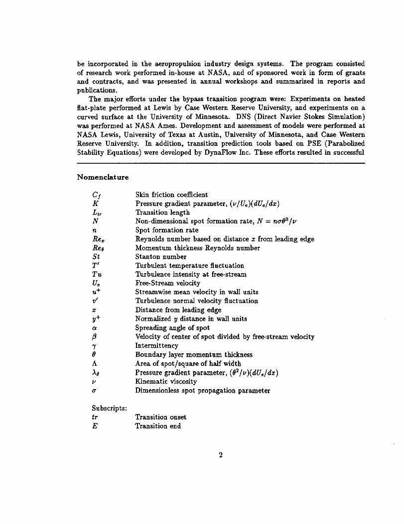
Nomenclature

C/K

LtrN

n

Rex

ReeStT'

Tu

u_u+

X

y+

3

70

A

he

V

ff

Subscripts:tr

E

Skin friction coefficient

Pressure gradient parameter, (v/Ue)(dUe/dx)

Transition length

Non-dimensional spot formation rate, N = naOa/v

Spot formation rate

Reynolds number based on distance x from leading edge

Momentum thickness Reynolds numberStanton number

Turbulent temperature fluctuation

Turbulence intensity at free-stream

Free-Stream velocity

Streamwise mean velocity in wall units

Turbulence normal velocity fluctuation

Distance from leading edge

Normalized y distance in wall units

Spreading angle of spot

Velocity of center of spot divided by free-stream velocity

Intermittency

Boundary layer momentum thickness

Area of spot/square of half width

Pressure gradient parameter, (O2/v)(dU_/dz)

Kinematic viscosity

Dimensionless spot propagation parameter

Transition onset

Transition end

generation of experimental and numerical databases, which contributed to understanding of

the flow physics, and served as a basis for model development and computational validation.

In 1994 the aero-propulsion industry expressed the need for efficiency improvements of

engine components characterized by low Reynolds number flows, such as the low-pressure

turbine (LPT). As transition plays a significant role in these flows, it was natural to respond

to this need by expanding the scope of the bypass transition program to include separation

and unsteady effects (wakes). Accordingly, the program was renamed The Low-Pressure

Turbine Flow Physics Program. To facilitate model development work, NASA Lewis chose

a management approach which strongly emphasizes collaboration and cooperation between

academic and research institutes, industry, and government laboratories. The technical ap-

proach continues to consist of combination of experimental work, computation, and analysis

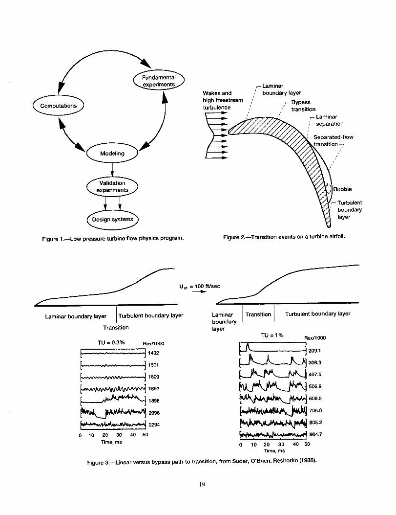
and modeling (figure 1).

The major research elements of the LPT program are currently underway. Experimental

work is in progress at Lewis with cooperation with University of Toledo, at University

of Minnesota, at the US Air Force Wright Laboratory, and is at the planning stage at

General Electric Aircraft Engines in Evandale, Ohio (GEAE). Computations are performed

by Western Michigan University, NASA Lewis, and CMOTT/OAI (Center for Modeling

of Turbulence and Transition/Ohio Aerospace Institute). Additional analysis is done by

collaboration between NASA Lewis, Syracuse University and GEAE, and by cooperation

between NASA Lewis and Pratt _ Whitney. Model development is performed at NASA

Lewis, Nyma Inc./Lewis Group, and CMOTT/OAI. Final validation of the models to be

developed will be made by implementing them in a CFD code and comparing to results

from future low-speed rotating rig experiments.

The significance of the work is mainly in two areas. The first one is a contribution to

temperature and life prediction of blades and vanes in the high-pressure turbine. Blade tem-

perature is an important design criterion which greatly affects the design and performance

of the whole engine. In addition, life cycle of components, directly affecting maintenance

cost is a major factor in design of jet engines. As life of blades is strongly affected by

their temperature, its accurate prediction is very important. The second area of signifi-

cance of this program is in reduction of the performance degradation from takeoff to cruise

operating conditions of the low-pressure turbine. The decrease in efficiency between the

two operation points is attributed to Reynolds number, which is higher at sea-level takeoff

conditions than at altitude cruise conditions. This problem affects mostly the low pressure

turbine where up to 2 percent efficiency differentials between takeoff and cruise may be en-

countered (Presentations at Heat Transfer Branch Bypass Transition Workshop 1993, LPT

Flow Physics Workshop, 1995). This gives jet-engine designers the potential for significant

efficiency improvements, which translate into fuel and weight savings.

It is then clear that improved modeling and understanding will contribute to more ac-

curate predictions of temperatures and losses, will allow turbine designers to quantitatively

compare alternative designs, and will impact overall engine design, performance, cost, and

marketability. Advanced CFD methods, such as Direct Navier Stokes Simulation (DNS),

or Large Eddy Simulations (LES) has progressed in recent years. These methods, which in

principlecanaddressverycomplexflows,arenot yet practicalto beusedin routinedesignsystems,thereforemodelingis still required.

It is clearthat the uniqueflow physicsin the turbine must be taken into accountindevelopingmodeling methods for adequate predictive capability. Figure 2 depicts the flowissues encountered in turbine blades. The turbomachinery flow environment differs greatly

from that of external aerodynamics. In external aerodynamics the incoming flow to the

airfoil is normally quiescent. Freestream turbulence levels are in the order of tenth of a

percent. In the gas turbine the flow enters the high pressure turbine from the combustor,

and the environment is characterized by high levels of turbulence, unsteadiness and flow in-

homogeneities. The flow in downstream stages and in the low-pressure turbine is dominated

by wake passing and the associated wake turbulence. There is little information available

in the open literature based on measurements of the turbulence in actual turbine. The

levels of turbine inlet turbulence can only be inferred from limited available measurements

of turbulence levels in the exit of the combnstor (Zimmerman,1979, Seasholtz et al, 1983,

Bicen and Jones, 1986, Ames and Moffat, 1990, Ames, 1994)

In low-level turbulence environment the transition process is initiated by linear mecha-

nisms. Freestream disturbances enter the boundary layer via mechanism called Receptivity

(see review by Reshotko, 1994), and generate linear instability waves (Tollmien-Schlichting

or GSrtler waves). The process is followed by a variety of possible nonlinear mechanisms

that lead to breakdown of the laminar boundary layer and to the generation of turbulent

spots. As the turbulent spots grow, the transitional boundary layer becomes a fully de-

veloped turbulent boundary layer. In a highly disturbed environment the linear stage is

bypassed and nonlinear stages are triggered directly. This transitional route to turbulence

is called Bypass Transition (Morkovin 1978a,b, 1993), and is recognized as the prevailing

transition mode in turbomachines. Figure 3 shows the differences between the mechanisms,

as reflected by hot wire measurements at low and high levels of freestream turbulence.

The development of the boundary layer over the blade is affected by a multitude of

factors. The major factors are the blade Reynolds number, freestream turbulence intensity

(and possibly scales, spectra etc.), pressure gradient, and curvature. At low to moderate

levels of turbulence there is a laminar region extending from the leading edge, sometimes

called the "buffeted boundary layer", "quasi-laminar", or "laminar-like" boundary layer.

The oscillations in this region caused by the freestream turbulence consist of linear and

nonlinear wave motions, and do not have turbulence characteristics.

The boundary layer may separate, particularly on the suction surface of the blade. Sep-

aration may occur in form of a bubble, or as massive separation with no reattachment

resulting in large losses. The pressure surface may have cove separation, and small separa-tion bubbles may exist near the leading edge. Often the separation bubble is transitional,

where transition starts in the local shear layer that develops at or near the separation point.

The reattachment is usually turbulent.

Wake passing was found to have important effects on the flow in turbomachinery (in

turbines as well as in compressors), as shown by the comprehensive work of Halstead et al

(1995). The wake interacting with the boundary layer creates a convected transitional or

4

turbulent patch, trailed by the "calmed" region, a relaxation region between the patch and

the the laminar boundary layer. The development of the boundary layer is determined by

the interplay between the transition, wake interaction, and separation mechanisms (see also

Cumpsty et al, 1995). Important additional factors that need to taken into account when

wakes are considered are the wake frequency parameter, and the turbine stages geometry.

It is also clear that properties of the wake turbulence and of the freestream turbulence play

an important role. It seems that in addition to the level of the turbulence, the scales and

perhaps the spectra of the turbulence need be considered. It needs to be noted that that

there is lack of information on the scales and spectra of freestream and wake turbulence.

Some relevant measurements were performed by Ames (1994), in turbine cascade withsimulated combustor.

Models are required to predict the onset point of transition and the transition region

itself. Separation needs to be predicted, including the location of the separation point and

the reattachment point. Transition in a separation bubble under conditions of freestream

turbulence has not been properly addressed yet. The effects of wake passing, particularly

the calmed region need to be incorporated. For example, when dealing with separation

it is important to know if the boundary layer transitions before the separation point, as

turbulent boundary layers delay separation. That is where the models for calculating bypass

transition in attached flow may be useful.

The following sections focus on describing the progress in modeling which was mostly

accomplished under the bypass transition program. Much of the progress will be directly

applied in the current challenging LPT Flow Physics Program.

RESEARCH PROGRESS

Transition Onset

Non wake-induced transition onset

Use of two-equation near-wall turbulence models has in general been successful in the pre-

diction of bypass transition onset. Simon and Stephens (1991) used the Jones-Launder

turbulence model to predict onset and compared their results with experimental data and

the correlation of Abu-Ghannam and Shaw (1980). The comparison of their results with the

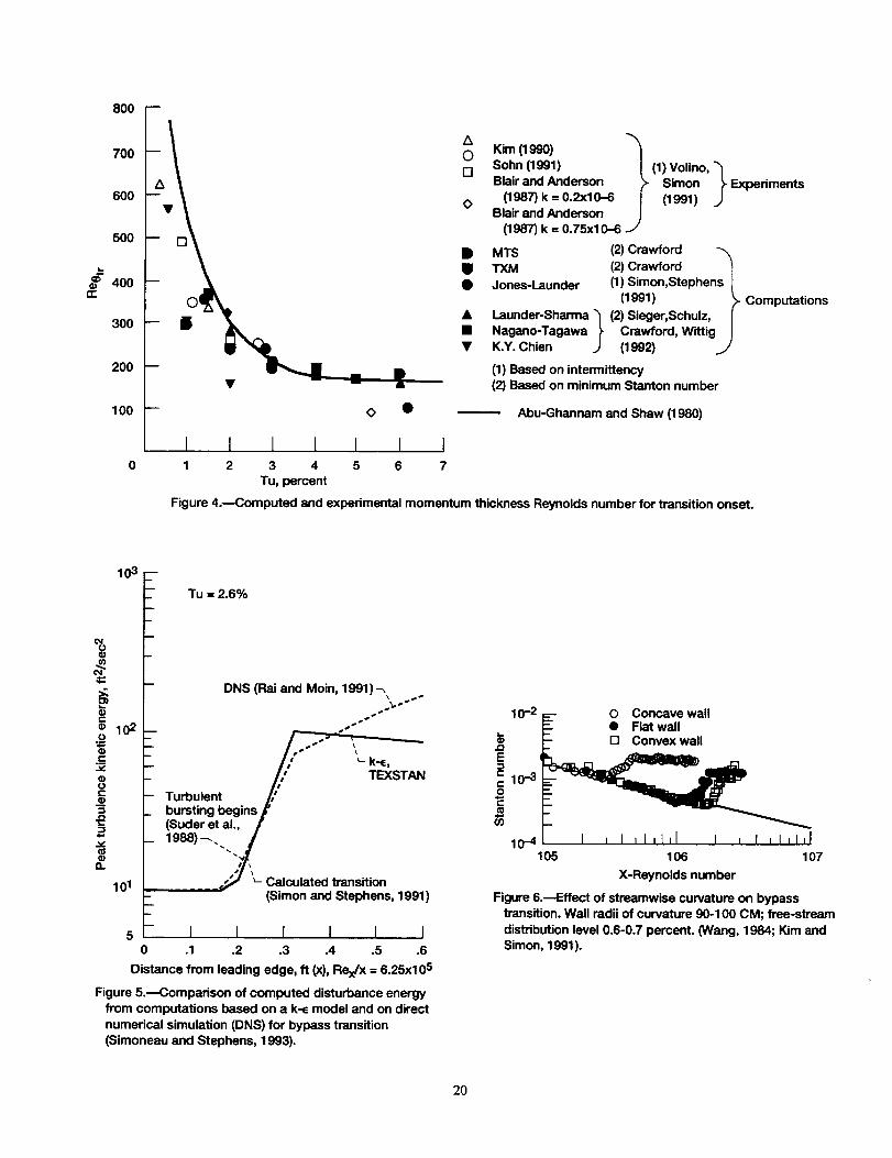
correlation of Abu-Ghannam and Shaw is good, as shown in figure 4. Simon and Stephens

(1991) assumed the transition onset to occur when the numerical computations indicated

a rapid increase in turbulence kinetic energy, indicating a non-zero intermittency. This

assumption was confirmed (Simoneau and Simon, 1993) by comparison with the DNS cal-

culations of Rai and Moin (1991) shown in figure 5 for the case of zero pressure gradient

and 2.6 percent freestream turbulence. Figure 5 shows how the two-equation turbulence

model captures the nonlinear disturbance growth which leads to the first sign of turbulent

spot formation. Suder, O'Brien and Reshotko's (1988) single-wire measurements within the

boundary layer indicated spot initiation at a boundary layer turbulence level of 3.5 percent

regardless of the path to transition (high or low freestream turbulence). This experimental

result appears consistent with the calculations of Simon and Stephens (1991) and _ and

Moin (1991) shown in figure 5.

Figure 5 suggests that, below a certain critical Reynolds number, amplification of dis-

turbances is not significant. This was the basis for the assumption made by Schmidt and

Patankar (1988) in their development of a turbulence model for transition and the basis used

by Simon and Stephens (1991) for initializing the calculations for disturbance energy shown

in figure 5. The assumption made by the above authors was that this critical Reynolds

number is close to the critical Reynolds number for linear instability.

Other experimental and analytical values for transition onset are given in figure 4.

The experimental transition onset values of figure 4 are based on the zero intermJttency

point, while the computational transition onset values are based on zero intermittency and

the minimum Stanton number. Figure 4 shows some experimental transition onset results

given in the survey report of Volino and Simon (1991) and some examples of the result

of transition onset calculations utilizing a number of turbulence models developed at the

University of Texas at Austin. Figure 4 shows the general applicability of turbulence models

for predicting transition onset. Turbulence models developed at the University of Texas at

Austin (Crawford, 1991) called the Texas model (TXM) and the Multi-Time-Scale (MTS)

model have the potential of improved simulation of the transition region. A multiple-scale

k-e turbulence model developed by Wu and Reshotko(1996) was found to predict transition

onset reasonably well.

The K.-Y. Chien turbulence model (1982) results shown in figure 4 were found by

Stephens and Crawford (1990) to give a premature value for transition onset. They ex-

plained that this is because the damping function of the Chien model is dependent only

on the boundary layer normal distance and that an improved onset prediction is obtained

when the damping function is dependent on the turbulent Reynolds number. The inability

of the K.-Y. Chien model to simulate transition onset was also found by the heat transfer

Navier-Stokes calculations of a turbine blade by Ameri and Arnone (1992).The effect of curvature on transition onset at low freestream turbulence is summarized

from the experimental work of Wang (1984) and Kim and Simon (1991) in figure 6. In

figure 6 the pressure surface of a turbine blade is represented by the concave surface and

the suction surface is represented by the convex surface. As indicated in figure 6, a convex

surface when compared to a fiat surface will delay transition onset and a concave surface

compared to a flat surface will shift transition onset upstream. The differences in onset

location, based on the minimum in the Stanton number, for a convex surface and a flat

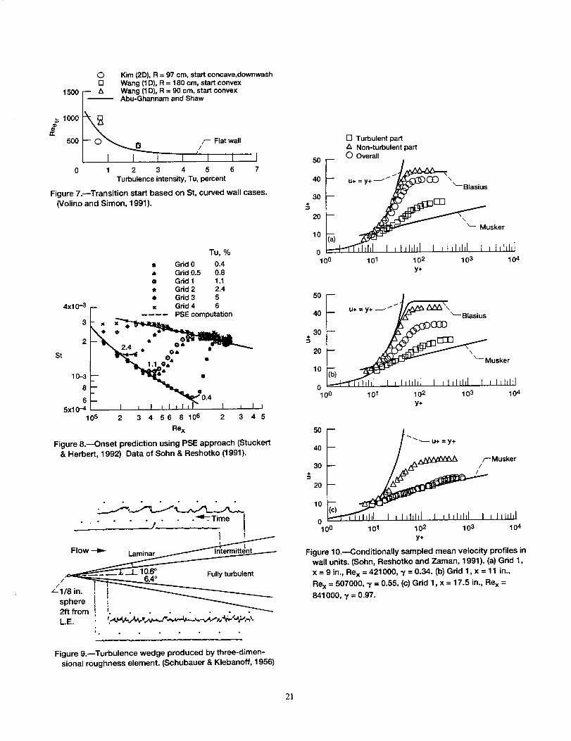
surface diminish as the freestream turbulence increases (figure 7). This suggests that for

the freestream turbulence levels encountered in an engine, curvature plays a minor role inthe value of transition onset on the suction surface of a turbine blade.

Volino and Simon (1991) noted little effect of favorable pressure gradient on the momen-

tum Reynolds number of transition. This is in agreement with findings of Abu-Ghannam

and Shaw (1980).

Stuckert and Herbert (1992) compared their Parabolized Stability Equations (PSE)

approachwith the experimental data of Sohn and Reshotko (1991) as shown in figure 8.

The onset of transition as defined by the minimum Stanton number is predicted very well

by the PSE method. Volino and Simon (1991) compared the zero intermittency point

with the minimum Stanton number (used by some as a definition for transition onset) anddetermined that the minimum Stanton number is located somewhat downstream of the zero

intermittency point. This was also noted by Simon and Stephens (1991).

Wake-induced transition onset

A reasonable estimate may be made of wake-induced transition onset by using the local value

of the wake turbulence intensity in the Abu-Ghannam and Shaw correlation. However,

the actual transition onset is generally lower than that predicted with the correlation of

Abu-Ghannam and Shaw (Orth, 1993), which approaches a momentum thickness Reynolds

number of 163 at high freestream turbulence. In general, the momentum thickness Reynolds

number for onset has a range of 90 to 150. Work needs to be done to establish a reliable

prediction of wake-induced transition onset.

Transition onset on a separated shear layer

As the blade Reynolds number is reduced, transition via laminar separation becomes more

prevalent than bypass transition. It is unlikely that transition on the separated shear

layer will begin with turbulent spots as occurs on an attached boundary layer (Gleyzes,

et al, 1985). Transition correlations, such as Roberts (1975) and Mayle (1991), have been

developed in terms of the distance from onset of separation to the end of transition. It is

often assumed that the momentum thickness Reynolds number changes very little between

separation and transition onset.

Effect of calmed region on transition onset

The calmed region is that region behind a turbulent spot or spots, generated by a freestream

or wake disturbance, that has the characteristic of decreasing but still elevated wall shear

stress producing a condition that suppresses new instabilities or turbulent spots. Only when

the calmed region returns to its original non-turbulent level does the possibility exist for

new turbulent spot onsets to begin. This effect can be seen in the hot-wire interrogation

of wedge flow by Schubaner and Klebanoff (1956) shown in figure 9. Figure 9 shows how

a new spot does not begin until the effects created by the old spot diminish. Schubauer

and Klebanoff state that transition will not occur in this region they label the "recovery

trail". This recovery trail or calmed region is seen in the time trace of figure 9 as a gradual

decrease in the signal with time. The effect of the calmed region is to lengthen the transition

region, a fact that will change the expected profile losses on a turbine or compressor blade,

as documented by Halstead, et al (1995).

Transition Region

Non wake-induced

Figure I0 shows conditionallysampled velocityprofilesin the transitionregion of a flat

plate as reported by Sohn, Reshotko and Zaman (1991). Figure 10 shows the departure

from a Blasiusprofileas an indicationof the transitionregion which occurs aftertransi-

tion onset. The deviationof the non-turbulentprofilesfrom the Blasiuscurve increases

with intermittency,while the turbulentpart of each profileapproaches the fully-turbu-

lentboundary layerprofileas intermittencyincreases.The deviationof the non-turbulent

part from a Blasiusprofilewith increasedintermittencyisattributedby Kim and Simon

(1991),as wellas by Sohn and Reshotko (1991),to a post-burstrelaxationperiod (calmed

region)requiredfor a disturbancein the non-turbulentpartof the flowto damp-out. With

an increasein the number of turbulentspots,or increasedintermittency,there are more

post-burstrelaxationperiodsincludedin the non-turbulentpartofthe flow.Figure 10 also

suggeststhat the transitionregioncannot be describedas a simpleintermittencyweighted

linearcombination of Blasiusand fully-turbulentboundary layerprofiles,as postulatedby

Dhawan and Narasimha (1958).

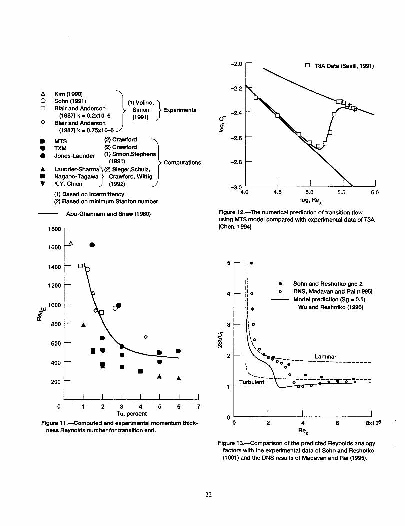
The momentum thickness Reynolds number at the end of transition, as compared with

the correlation of Abu-Ghannam and Shaw (1980), is given in figure 11. Figures 4 and 11

demonstrate the strong effect freestream turbulence intensity plays, although it is expected

that the spectra and length scale of the freestream turbulence will be needed to further

refine the turbulence effects. While k - _ turbulence models perform well in the prediction

of transition onset (figure 4), they generally give an underprediction of transition length

(figure 11). A reason for this may be found in the work of Volino and Simon (1993). Volino

and Simon (1993) applied an octant analysis to the experimental data to analyze the differ-ence in structure between turbulent and transitional flows. They indicate that transitional

boundary layers show incomplete mixing or incomplete development of turbulence with a

domination of the large scale eddies. This is attributed to the incomplete development of

the cascade of energy from large to small scales. Based on this observation, it is stated that

the standard k - e turbulence model does not comprehend the physics of the transition

region and what is needed is a model that will comprehend both large and small scales

separately. This would require a modified k - 6 equation with perhaps two equations for

the turbulent kinetic energy (k); one k -e equation for the large scale eddies and one for the

small scale eddies. Such a multi-time-scale (MTS) model for application to transition flows

has been implemented by Crawford (1992). This model is an evolution of two-scale k - E

models developed by Hanjalic, Launder and Schiestel (1980) and Kim (1990). Numerical

calculations performed by Chen (1994) at the University of Texas (figure 12) show promise

that the MTS model is capable of simulating the transition region for turbulence levels

greater than two percent. A similar approach utilizing a multiple scale k - e turbulence

model was reported by Wu and Reshotko (1996). One of their results (figure 13) for the

Reynolds analogy factor shows an early transition but agrees well in the fully turbulent

flow. The Reynolds analogy results of figure 13 reflect the unheated starting length of 1.375

8

inches of the experiment.

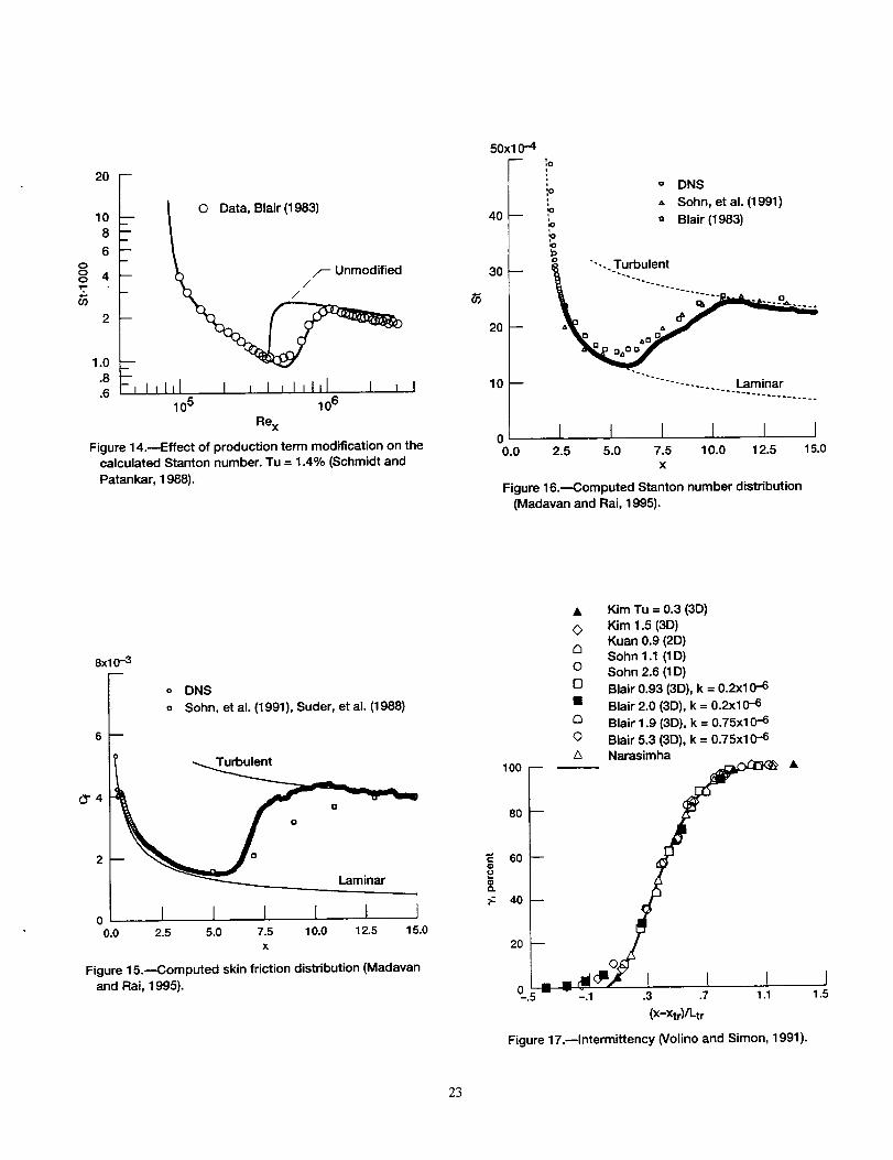
Schmidt and Patankar (1988) attributed the underprediction of the transition length to

the production term of the turbulent kinetic energy equation. They modified the production

term to make predictions consistent with experimental results. Figure 14 demonstrates the

improved prediction of transition as a result of modifying the production term.

A DNS calculation of transition on a heated flat plate, for a freestream turbulence of

2.6% , was performed by Madavan and RaJ (1995). Madavan and Rai used a high-order-

accurate finite-differencing approach for the direct numerical simulation of transition and

turbulence. Figures 15 and 16 compare the skin friction and Stanton number experimental

results of Suder, O'Brien and Reshotko (1988), Sohn and Reshotko (1991), and Blair (1983),

with the DNS results. There is reasonable agreement between experiment and DNS results,

with the agreement being better for the heat transfer results. The results for the Reynolds

analogy were shown in figure 13. There is good agreement in the laminar and turbulent

regions. The difference between calculation and experiment in the transition region is due to

the rapid increase in the calculated skin friction (figure 15). Sufficient confidence has been

established with the DNS approach that the resulting numerical base is seen as valuable

for the development and testing of turbulence models applicable to bypass transition. As

a point of interest, the experimental work of Sohn and Reshotko (1991) reported negative

values for the turbulent heat flux (v-r_T_) near the wall in the transition region. The attempts

to experimentally determine the reason for this anomaly (Sohn, Zaman, and Reshotko,

1992) have not been successful. The DNS results of Madavan and Rai show no evidence of

negative turbulent heat flux for either the transition or turbulent region. This discrepancy

demonstrates the challenges associated with validating results of hot-wire measurementsnear the wall.

Simon and Stephens (1991), following the concept of Schmidt and Patankar, utilized

stability considerations for determining the location of the initial profiles in the numeri-

cal calculations, and developed a basis for utilizing intermittency in transition calculations.

They followed the method of Vancoille and Dick (1988) to develop conditional averaged tur-

bulence model equations for heat transfer. This approach is felt to be better than a global

time average approach which does not take into account a transition zone consisting of tur-

bulent spots surrounded by laminar-like fluid. The method of Simon and Stephens (1991)

assumes the universal intermittency relationship of Narasimha (1957) which compares fa-

vorably with the experimental data as presented by Volino and Simon (1991) aald shown in

figure 17. As can be seen on figure 17, a determination of intermittency requires knowledge

of the transition length. This was done by Simon and Stephens by utilizing the approach of

Narasimha (1985) which expresses the transition length in terms of a nondimensional spot

formation rate (N). Narasimha (1985) demonstrates that N reaches a constant value at

the higher turbulence levels. The experimental value of N used by Simon and Stephens was

compared to the result of an analysis by Simon (1994). The following equation of Simon

(1994) relates N to turbulent spot characteristics:

N = (Atana) 2 8.ix IO (I)

9

The analytical value of N reported by Simon (1994) using equation (1) is a constant of

0.00029 (zero pressure gradient), in agreement with the experimental value. The use of N

permits a determination of transition length by means of the following equation reported

by Simon and Stephens (1991):

2.15 ,_

Re L,, -- -_ _eo,, (2)

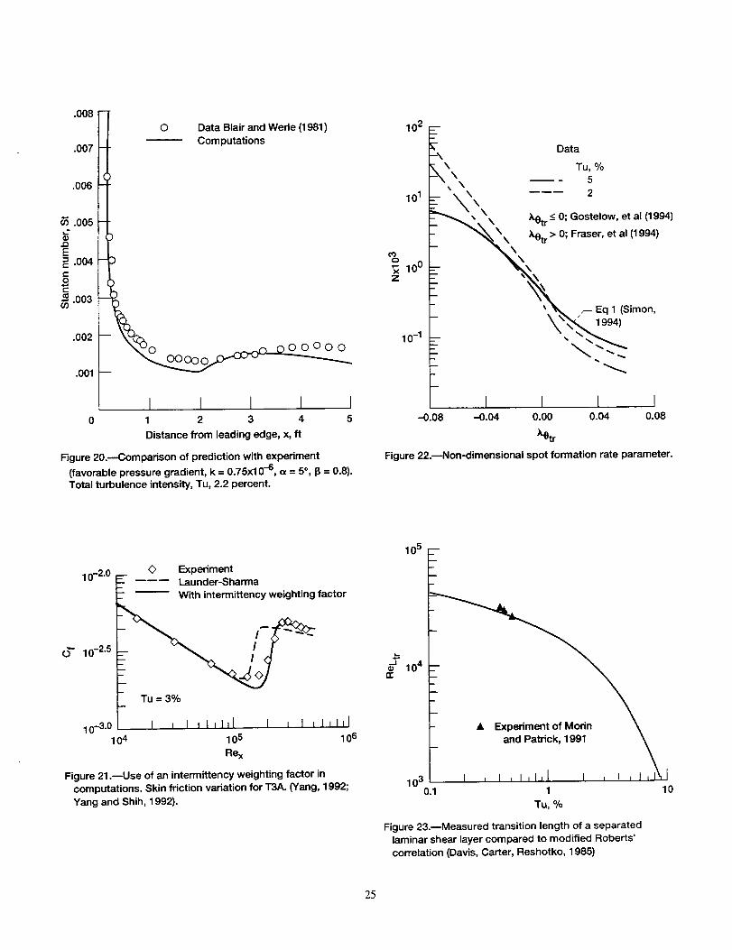
Transition calculations were made by Simon (1994) utilizing equations (1) and (2), and

the intermittency path equation of Narasimha (1957) with the TEXSTAN code of Crawford

(1985). The resulting calculations are compared to the data of Blair and Werle (1980, 1981)

in figures 18 to 20 for zero and favorable pressure gradients. Figure 18(a) is an example of the

abrupt onset of transition that was obtained when intermittency was not used. The value

of using intermittency for improvement of the transition model is clearly demonstrated.

There is generally good agreement between experiment and prediction. It is interesting to

note, according to the calculations, that the boundary layer acts as if it were a laminar

boundary layer up to a significant value of the intermittency (figure 19). This is consistent

with the measured velocity profiles of Sohn, O'Brien and Reshotko (1989) which showed a

laminar-like overall profile in the transition region for intermittency values up to 0.34 at 1

percent freestream turbulence.

Yang and Shih (1992) Report an improvement over the Launder-Sharma model (Launder

and Sharma, 1974) by the use of a new low-Reynolds-number turbulence model and an

intermittency weighing factor. The intermittency weighing factor used by Yaag and Shih

is related to an intermittency factor defined by the variation of the boundary layer shape

factor through the transition region. The intermittency weighing factor is used to modifythe calculated eddy viscosity in the transition region. The result is an improvement over

the Launder-Sharma model, as shown in figure 21. In addition, Yang and Shih point out

that a drawback of the Launder-Sharma model is its inability to perform as well as other

models for fully-developed turbulent boundary layers.

Solomon, Walker and Gostelow (1995) propose a new calculation method for inter-

mittency that allows for adjustment of spot growth'parameters in response to changes in

the local pressure gradient. This especially valuable for turbomaz.hinery flows where large

changes in pressure gradient occur within the transition region. The method permits a more

accurate value of intermittency for use in eddy viscosity methods such as the Simon and

Stephens (1991) method noted above. Solomon, et al (1995) present the following equation:

"y = l - exp -n tan a dz (3)t

The spot formation rate (n), spot propagation parameter (a) and turbulent spot spreading

angle (a) are presented as correlations (Gostelow et al, 1994, 1995) in terms of a pressure

gradient parameter (Ae). The spot formation parameter is calculated from the correlation

for the non- dimensional spot formation rate parameter (N). This correlation is a function

of pressure gradient and freestream turbulence. A comparison of the Gostelow et al (1994)

10

correlation for N at a freestream turbulence of 2 and 5 percent is made with equation

(1) in figure 22. The calculation with equation (1) employed the spot spreading angle

correlation of Gostelow, et a/(1995). A value of A = 2.88 was used in equation (1), and

was determined with the correlations for turbulent spot spreading angles and velocities for

a zero pressure gradient. Figure 22 shows a fair comparison between equation (1) and the

Gostelow correlation. The divergence at the higher adverse pressure gradients is expected as

the transition region for these pressure gradients is more governed by streamwise interaction

of turbulent spots (Walker, 1987) while equation (1) was derived assuming lateral interaction

of spots. The value of N in figure 22 for a zero pressure gradient, using equation (1), is 66_

greater than indicated above (Simon, 1994), due to the spot properties given by Gostelow.

Wake-induced transition

Addison and Hodson (1991) state that wake-induced transition can be treated in the same

manner as steady transition. Therefore, it can be assumed that turbulent spots created by

the presence of unsteady disturbances, and the resulting intermittency, can be described

by equation (3) above and the steady state correlations of Gostelow, et al (1994, 1995).

It would appear that the computational method of Solomon, Walker and Gostelow (1995)

is applicable here. The other approach is to use intermittency equations developed, for

wake-induced transition, by Mayle and Dullenkopf (1989, 1991) and Hodson, et al (1992).

In either case the key variable required for intermittency calculations is the location of

transition onset. As indicated above, more work is needed in the area of wake-inducedtransition onset.

Separated-flow transition

Mayle (1991) provides an excellent summary of separated-flow transition and notes its im-

portance to the design of low-pressure turbines. The resulting bubble formation of separated

flow can have a significant effect on the aerodynamics and heat transfer of turbines. There

is a need to predict laminar boundary layer separation with turbulent reattachment, deter-

mine the bubble's displacement effect on the mainstream flow and whether the bubble will

"burst" and dramatically increase the blade losses. It is important to know something of

the separated layer transition process for a determination of bubble length and "bursting".

Some progress toward meeting this need was provided by a NASA sponsored experimental

study of the bubble formation process for a "short" laminar bubble (Morin and Patrick,

1991). Morin and Patrick provide detail measurements of a laminar separation bubble and

compare the measured transition length to existing correlations. Figure 23 shows a com-

parison of the experimental transition length with a modified Roberts correlation (Davis,

Carter, and Reshotko, 1985). There is excellent agreement in the limited range of freestream

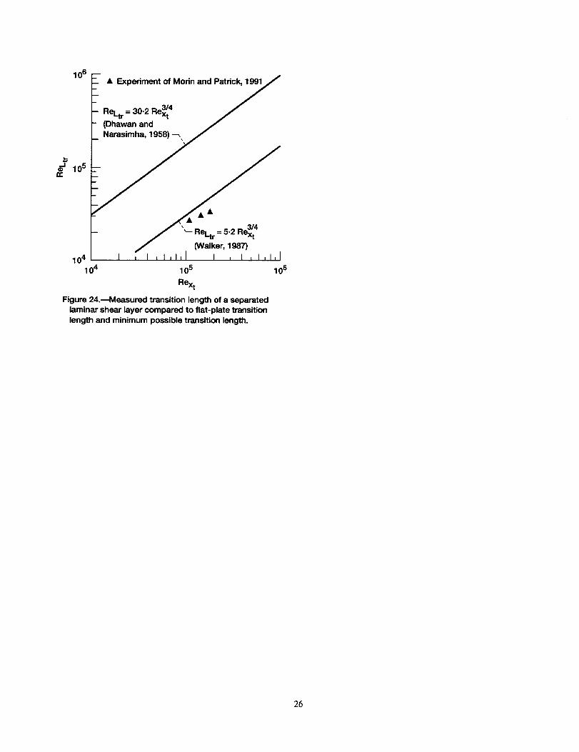
turbulence used. Walker (1987) indicates that the transition length for a separated laminar

shear layer should be less than that for an attached boundary layer and greater than that

predicted by his model for a minimum transition length at zero pressure gradient. His cor-

relation of the minimum transition length compares favorably and slightly higher than the

11

experimentaldataasshownin figure24. The transitionlengthfor an attachedboundarylayer,as predicted by Dhawan and Narasimha (1958) is about an order of magnitude greaterthan the measured values on a separated laminar shear layer. Walker's analysis is based on

the interaction of turbulent spots in the streamwise direction. Further study is required to

determine the applicability of a turbulent spot model on a separated laminar shear layer.

Effect of the calmed region

An excellent documentation of the effect of the calmed region on transition and separation

is provided by the experimental and numerical work of Halstead, et al (1995). Their results

show the suppression of laminar separation and the delay of transition onset as noted above.

The separation that was expected on a compressor or turbine blade did not occur due to

the elevated shear stress produced by calming. The effect of the calmed region to extend

the transition zone and suppress separation can have a profound impact on the design

of low-pressure turbines. The interplay between wake frequency and the calming region

is interesting. Halstead, et al, have observed on a compressor blade that when the wake

frequency is high enough, so that the calming region does not decay to zero before the next

wake, bypass transition dominates. When the wake frequency decreases, the calming effects

also decrease, and separated flow transition dominates. Orth (1993) noted that laminar

calmed regions, behind turbulent patches created by wakes, existed far beyond the location

at which the undisturbed boundary layer is fully turbulent. The work of Ha]stead, et al

(1995), as well as of other researchers, points out the need for additional studies of the

calmed region and for the development of unsteady models that will comprehend the effect

calming has on transition and separation. This need is best expressed with a quote from

Halstead, et al (1995); "Improvements in modeling the essential physics of turbulent spot

formation and the associated calmed effects as well as addressing flow separation issues

would likely improve predictions".

CONCLUDING REMARKS

This research progress report has demonstrated the importance of a team approach, with

the appropriate mix of experimental and analytical skills, for the purpose of understanding

and modeling the complex physics occurring on a turbine blade. Sufficient progress has

been made in the understanding and modeling of Bypass Transition so that specific recom-

mendations may be made for modeling non wake-induced transition onset. Two-equation

turbulence models appear to capture the growth of non-linear disturbances in bypass tran-

sition and are capable, with appropriate damping functions and constants, of predicting

transition onset. However, these models under-predict the transition length unless, (1) pro-

vision is made for the intermittent nature of the transition region, or (2) a modification is

made for the rate of turbulence production, or (3) a multi-scale model is used to account for

the incomplete nature of the turbulent energy cascade in the transition region. The needfor a multi-scale turbulence model has been confirmed by an analysis of the experimental

12

data.A recommendation is made for the use of the intern_ttency calculation approach of

Solomon, Walker and Gostelow (1995) in the transition region to permit the proper tur-

bulent spot growth as a function of the local pressure gradient on a turbine blade. It has

been demonstrated that the use of intermittency in the numerical calculations is the most

effective approach for modeling of the transition region.

Direct Numerical Simulation (DNS) has proven to be a very powerful tool for under-

standing the physics, supporting and guiding the experimental results and forming a data

base for the development and testing of transition turbulence models. Results obtained

with DNS compare very well to the experimental results.

A great deal more effort needs to be applied to the understanding and modeling of the

effect that the calmed region has on transition and separation, transition on a separated

shear layer, and wake-induced transition.

REFERENCES

Abu-Ghannam, B.J. and Shaw, R. 1980. Natural Transition of Boundary Layers - The

Effects of Turbulence, Pressure Gradient, and Flow History, J. Mech. Engr. Sci.,

22(5), 213-228.

Addison, J.S. and Hodson, H.P. 1991. Modelling of Unsteady Transitional Boundary

Layers, ASME Paper 91-GT-282.

Ames, F.E. 1994. Experimental Study of Vane Heat Transfer and Aerodynamics at

Elevated Levels of Turbulence, NASA CR-4633.

Ames, F.E. and Moffat, R.J. 1990. Heat Transfer With High Intensity, Large Scale

Turbulence: The Flat Plate Boundary Layer and the Cylindrical Stagnation Point,

Report No. HMT-43, Thermosciences Division of Mechanical Engineering, Stanford

University.

Ameri, A.A. and Arnone, A. 1992. Navier-Stokes Turbine Heat Transfer Predictions

Using Two-Equation Turbulence Closures, NASA TM 105817.

Bicen, A.F. and Jones, W.P. 1986. Velocity Characteristics of Isothermal and Combusting

Flows in a Model Combustor, Combust. Sci. and Technology, 49, 1-15.

Blair, M.F. 1983. Influence of Free-Stream Turbulence on Turbulent Boundary Layer

Heat Transfer and Mean Profile Development, Part 1, Experimental Data, ASME

Journal of Heat Transfer, 105, 33-40.

Blair, M.F. and Anderson, O.L. 1987. Study of the Structure of Turbulence in Acceler-

ating Transitional Boundary Layers, UTRC report R87-956900-1.

13

Blair, M.F. and Werle, M.J. 1980. The Influence of Free-Stream Turbulence on the Zero

Pressure Gradient Fully Turbulent Boundary Layer, UTRC report R80-914388-12.

Blair, M.F. and Werle, M.J., 1981. Combined Influence of Free-Stream Turbulence and

Favorable Pressure Gradients on Boundary Layer Transition, UTRC Report R81-

914388-17.

Chen, T.-H. 1994. Numerical Simulation of Bypass Transition Using Two-F._luation and

Multiple-Time-Scale Models, Doctor of Philosophy Dissertation, University of Texasat Austin.

Chien, K.-Y. 1982. Predictions of Channel and Boundary-Layer Flows with a Low-

Reynolds-Number Turbulence Model, AIAA Journal, 20, 33-38.

Crawford, M.E. 1985. TEXSTAN program, University of Texas at Austin.

Crawford, M.E. 1991. Progress Report of NASA Grant NAG3-864.

Crawford, M.E. 1992. Progress Report of NASA Grant NAG3-864.

Cumpsty, N.A., Dong, Y. and Li, Y.S. 1995. Compressor Blade Boundary Layers in

Presence of Wakes, ASME Paper 95-GT-443, International Gas Turbine Congress,Houston.

Davis, R.L., Carter, J.E. and Reshotko, E. 1985. Analysis of Transitional Separation

Bubbles on Infinite Swept Wings, AIAA Paper 85-1685.

Dhawan, S. and Narasimha, R. 1958. Some Properties of Boundary Layer Flow During

Transition From Laminar to Turbulent Motion, J. Fluid Mech., 3, 418-436.

Fraser, C.J., Higazy, M.G. and Milne, J.S. 1994. End-Stage Boundary Layer Transition

Models for Engineering Calculations, Proceedings of the Institution of Mechanical

Engineers, C208, 47-58.

Gaugler, R.E. 1981. Some Modifications to, and Operational Experience with, the

Two-Dimensional, Finite-Difference, Boundary Layer Code, STANS. ASME Paper

81-GT-89 (Published also as NASA TM 81631).

Gaugler, R.E. 1985. A Review and Analysis of Boundary Layer Transition Data for

Turbine Application, ASME Paper 85-GT-83.

Gleyzes, C., Cousteix, J. and Bonnet, J.L. 1985. Theoretical and Experimental Study

of Low Reynolds Number Transitional Separation Bubbles, Proe. Conf. on Low

Reynolds Number Airfoil Aerodynamics, Notre Dame, IN (T.J. Mueller, ed.), UNDAS-

CP-77B123, 137-152.

14

Gostelow, J.P., Blunder, A.R. and Walker, G.J., 1994. Effects of Free-Stream Turbulence

and Adverse Pressure Gradients on Boundary Layer Transition, ASME Journal of

Turbomachinery, 116, 392-404.

Gostelow, J.P., Melwani, N. and Walker, G.J. 1995. Effects of a Streamwise Pressure

Gradient on Turbulent Spot Development, ASME Paper 95-GT-303, International

Gas Turbine Congress, Houston.

Graham, R.W. (Ed.) 1985. Transition In Turbines, NASA CP-2386.

Halstead, D.E., Wisler, D.C., Okiishi, T.I,I., Walker, G.J., Hodson, H.P. and Shin, H.-W.

1995. Boundary Layer Development in Axial Compressors and Turbines, ASME

Papers 95-GT-461, 462, 463, 464 (Parts 1-4), International Gas Turbine Congress,Houston.

I-Ianjalic, K., Launder, B.E. and Schiestel, R. 1980. Multiple-Time-Scale Concepts in

Turbulent Transport Modelling, Turbulent Shear Flows, 2, Springer-Verlag, New York.

Hodson, H.P., Addison, J.S. and Shepherdson, C.A. 1992. Models for Unsteady Wake-

Induced Transition in Axial Turbomachines, Jnl. de Physque 2(4), 545-574.

Kim, S.-W. 1990. Numerical Investigation of Separated Transonic Turbulent Flows With

a Multiple-Time-Scale Turbulence Model, NASA TM 102499.

Kim, J. and Simon, T.W. 1991. Free-Stream Turbulence and Concave Curvature Effects

on Heated, Transitional Boundary Layers, NASA CR 187150.

Launder, B.E. and Sharma, B.I. 1974. Application of the Energy-Dissipation Model of

Turbulence to the Calculation of Flow Near a Spinning Disc, Letters in Heat and Mass

Transfer, 1,131-138.

Madavan, N.K. and Rai, M.M. 1995. Direct Numerical Simulation of Boundary Layer

Transition on a Heated Flat Plate with Elevated Freestream Turbulence, AIAA Paper95-0771.

Mayle, R.E. and DuUenkopf, K. 1989. A Theory for Wake-Induced Transition, J. Turbo-

machinery, 112, 188-195.

Mayle, R.E. and Dullenkopf, K. 1991. More on the Turbulent-Strip Theory for Wake-

Induced Transition, Transactions of the ASME, 113.

Mayle, R.E. 1991. The Role of Laminar-Turbulent Transition in Gas Turbine Engines,

ASME Paper 91-GT-261, International Gas Turbine Congress, Orlando.

Morin, B.L. and Patrick, W.P. 1991. Detailed Study of a Large-Scale Laminar Separation

Bubble on a Flat Plate, United Technologies Research Center Report K91-956786-1,NASA Contract NAS3-23693.

15

Morkovin, M.V. 1978a. InstabilityTransitionto Turbulence and Predictability,AGARD

AG-236 (availablefrom NTIS, AD-A057834).

Morkovin, M.V. 1978b. Bypass Transition to Turbulence and Research Desiderata, in

Transition In Turbines, NASA CP-2386, 161-204.

Morkovin, M.V. 1993. Bypass Transition Research: Issues and Philosophy, in Instabilities

and Turbulence in Engineering Flows (D.E. Ashpis, T.B. Gatski, and R. Hirsh, Eds.),

Kluwer Academic Publishers, Dordrecht, The Netherlands, 3-30.

Narasimha, R. 1957. On the Distributionof Intermittencyin the TransitionRegion of a

Boundary Layer,J. AeronauticalScience,24(9),711-712.

Narasimha, R. 1985. The Laminar-Turbulent Transition Zone in the Boundary Layer,

Progress in Aerospace Science, 22, 29-80.

Orth, U. 1993. Unsteady Boundary-Layer Transition in Flow Periodically Disturbed by

Wakes, Journal of Turbomachinery, 115, 707-713.

Rai,M.M. and Moin, P. 1991. DirectNumerical SimulationofTransitionand Turbulence

in a SpatiallyEvolving Boundary Layer,AIAA 10th Computational Fluid Dynamics

Conference,Honolulu,Hawaii,AIAA-91-1607.

Reshotko, E. 1994.94-0001.

Boundary Layer Instability, Transition and Control, AIAA Paper

Roberts, W.B. 1975. The Effect of Reynolds Number and Laminar Separation on Axial

Cascade Performance, Trans. ASME, J. Eng. Power, 261-274.

Savill, A.M. 1991. Turbulence Model Predictions for Transition under Free-Stream Tur-

bulence, RAeS Transition and Boundary Layer Conference, Cambridge, England.

Schmidt, R.C. and Patankar,S.V. 1988. Two-Equation Low-Reynolds-Number Turbu-

lence Modeling Of TransitionalBoundary Layer Flows Characteristicof Gas Turbine

Blades,NASA CR 4145.

Schubauer, G.B. and Klebanoff, P.S. 1956. Contributions on the Mechanics of Boundary

Layer Transition, NACA Report 1289.

Seasholtz R.G., Oberle, L.G. and Weikle, D.H. 1983. Laser Anemometry for Hot Section

Applications. Turbine Hot Section Technology, NASA CP-2289, 5?-6?.

Sieger, K., Schulz, A., Crawford, M.E. and Wittig, S. 1992. Comparative Study of Low-

Reynolds Number k-E Turbulence Models for Predicting Heat Transfer along Turbine

Blades with Transition, Presented at: International Symposium on Heat Transfer in

Turbomachinery, Athens, Greece.

16

Simon, F. 1994. The Use of Transition Region Characteristics To Improve the Numerical

Simulation of Heat Transfer in Bypass Transitional Flows, NASA TM 106445.

Simon, F.F. and Stephens, C.A. 1991. Modeling of the Heat Transfer in Bypass Transi-

tional Boundary-Layer Flows, NASA TP 3170.

Simonean, R.J. and Simon, F.F. 1993. Progress Towards Understanding and Predicting

Heat Transfer in the Turbine Gas Path, Int. J. of Heat and Fluid Flow, 14(2), 106-128.

Sohn, K.-H., O'Brien J.E. and Reshotko, E. 1989. Some Characteristics of Bypass

Transition in a Heated Boundary Layer, NASA TM 102126.

Sohn, K.-H. and Reshotko, E. 1991. Experimental Study of Boundary Layer Transition

With Elevated Freestream Turbulence on a Heated Flat Plate, NASA CR 187068.

Sohn, K.-H., Reshotko, E. and Zaman, K.B.M.Q. 1991. Experimental Study of Boundary

Layer Transition on a Heated Flat Plate, NASA TM 103779.

Sohn, K.-H., Zaman, K.B.M.Q. and Reshotko, E. 1992. Turbulent Heat Flux Measure-

ments in a Transitional Boundary Layer, NASA TM 105623.

Solomon, W.J., Walker, G.J. and Gostelow, J.P. 1995. Transition Length Prediction for

Flows with Rapidly Changing Pressure Gradients, ASME Paper 95-GT-241, Interna-

tional Gas Turbine Congress, Houston.

Stephens, C.A., and Crawford, M.E. 1990. An Investigation into the Numerical Predictionof Boundary Layer Transition Using the K.Y Chien Turbulence Model, NASA CR

185252.

Stuckert, G.K. and Herbert, T. 1992. Transition and Heat Transfer in Gas Turbines,

Final Report, SBIR Contract NAS3-26602, NASA/Lewis.

Suder, K.L., O'Brien, :I.E. and Reshotko, E. 1988. Experimental Study of Bypass Tran-

sition in a Boundary Layer, NASA TM 100913.

Vancoillie, G. and Dick, E. 1988. A Turbulence Model for the Numerical Simulation of

the Transition Zone in a Boundary Layer, Int. J. Eng. Fluid Mech., 1, 28-49.

Volino, l_.J. and Simon, T.W. 1993. An Application of Octant Analysis to Turbulent and

Transitional Flow Data, IGTI ASME Turbo Expo, Cincinnati, Ohio, May 24-27,1993.

Volino, R.J. and Simon, T.W. 1991. Bypass Transition in Boundary Layers Including

Curvature and Favorable Pressure Gradient Effects, NASA CR 187187.

Walker, G.J. 1987.87-0010.

Transitional Flow on Axial Turbomackine Blading, AIAA Paper

17

Wang, T. 1984. An Experimental Investigation of Curvature and Free-free-stream Turbu-lence Effects on Heat Transfer and Fluid Mechanics in Transitional Boundary Layers,

PhD Thesis, Dept. of Mech. Engr., University of Minnesota.

Wn, S.-Y. and Reshotko, E. 1996. Multiple-Scale k - _ Turbulence Model of the Transi-

tional Boundary Layer for Elevated Freestream Turbulence Levels, NASA Contractor

Report, to appear.

Yang, Z. 1992. Modeling of Near Wall Turbulence and Modeling of Bypass Transition,

Center for Modeling of Turbulence and Transition (CMOTT): Research Briefs, (W.W.

Liou, ed.), NASA TM-105834, 83-94.

Yang, Z. and Shih, T.-H. 1992. A k- _ Calculation of Transitional Boundary Layers,NASA TM 105604.

Zimmerman, D.R. 1979. Laser Anemometer Measurements at the Exit of a T63-C20

Combustor. NASA CR-159623.

18

Modeling

Validation

experiments

systems

Figure 1.--Low pressure turbine flow physics program.

r- Laminar

Wakes and ,' boundary layerI

high freestream , ,-- Bypassturbulence ] ,' transition

j separation

Separated-flow

Bubble

Turbulent

boundary

layer

Figure 2.--Transition events on a turbine airfoil.

fI

Laminar boundary layer I Turbulent boundary layer

Transition

_ U==100ft/se_

I Transition I Turbulent boundary layer

TU = 0.3% Rex/1000

Laminar

boundary

layer

_,__ 1501

1600

_J_J_ 1693

--_'__ 1898

2096

2294

0 10 20 3O 4O 50

Time, ms

TU = 1% Rex/1000

_ 209.1308.3

i_*'__ 407.5

_ 506.9

_ 606.5

_ 706.0

_ 805.2

_ 904.7

0 10 20 30 40 5OTime, ms

Figure 3.--Linear versus bypass path to transition, from Suder, O'Brien, Reshotko (1988).

]9

n-

800

700

6OO

500

t_

4OO

3OO

200

100 O

I0 1 2 3 4 5 6

Tu, percent

Z_Kim (1990)

O Sohn (1991) | (1) Volino, _L[] Blair and Anderson _> Simon J(1987) k = 0.2x10-6 | (1991)O Blair and Anderson J

(1987) k = 0.75xl 0-6 J"

• MTS (2) Crawford -_

• TXM (2) Crawford(1) Simon,Stephens 1

• Jones-Launder (1991) _>

• Launder-Sharma _ (2) Sieger, Schulz, |

• Nagano-Tagawa _ Crawford, WittigJ• K.Y. Chien (1992) _/

(1) Based on intermittency

(2) Based on minimum Stanton number

Abu-Ghannam and Shaw (1980)

Experiments

Computations

I7

Figure 4.---Computed and experimantal momentum thickness Reynolds number for transition onset.

04O

¢:

G)p,Q)O

.m¢)

G)

-5

a.

10s-

p

m

Tu = 2.6%

DNS (Rai and Moin, 1991)-_

102 -- -- ,-°'"

_ // TEXSTAN

- Turbulent //_ bursting begins F

(Suder et al., /r

1988) ..,_f

I',101 _ _- Calculated transition

- (Simon and Stephens, 1991)

s - I n I I I I0 .1 .2 .3 .4 .5 .6

Distance from leading edge, ft (x), Rex/x = 6.25x105

Figure 5.--Comparison of computed disturbance energyfrom computations based on a k-_ model and on direct

numerical simulation (DNS) for bypass transition

(Simoneau and Stephens, 1993).

10 -2 O Concave wall

F • Flat walle_

e-o

lO-4105 106 107

X-Reynolds number

Figure 6.--Effect of streamwise curvature on bypasstransition. Wall radii of curvature 90-100 CM; free-stream

distribution level 0.6-0.7 percent. (Wang, 1984; Kim and

Simon, 1991).

20

O Kim (2D), R = 97 cm, start concave, downwash[] Wang (1D), R = 180 cm, start convex

1500 -- Z_ Wang (1D), R = 90 crn, start convexAbu-Ghannam and Shaw

1000 _500 //-- Flat wall

i i t i _l I I0 1 2 3 4 5 6 7

Turbulence intensity, Tu, percent

Figure 7.--Transition start based on St, curved wall cases.

(Volino and Simon, 1991).

Tu, %

• Grid 0 0.4• Grid 0.5 0.8• Grid I 1.1• Grid 2 2.4• Grid 3 5

4x10-3 r- x Grid 4 6| .... PSE computation

3k. 2 I-_ o_ * ,.,.a_'JMl_

I "'_._'_- _" ,_'_-'--I -'_ !._o,

5x10-4105 2 34 56 8106 2 3 45

Rex

Figure 8._Onset prediction using PSE approach (Stuckert& Herbert, 1992) Data of Sohn & Reshotko (1991).

• . _ Time II

I t

FIo _ 'w_

Fu,,yturbo,ent/ "

z- l/t_ In , " -

spnere I ! "2/tfrom ! _.......L.E. t,'_U'_-'&_'_"J"_"_-_"'_x,'V_J",_', "_"

;.

Figure 9.--Turbulence wedge produced by three-dimen-

sional roughness element. {Schubauer & Klebanoff, 1956)

5O

40

30

20

10

010 o

[] Turbulent partZ% Non-turbulent partO Overall

p

u+ = y+ _ \_Blasius

_usker

i lllllll I It111111 I I tltllll101 102 103 104

y+

50

40

30

20

10

010 o

-- u+=y+ _tT_/VV_\ \

- //_-'- _Slasius

__-- _Musker

(b),--,.6,'l'T_lm( I _ IIi iI_[ I _hlll_l I _ ILIIIII

1o1 10 2 103 10 4

Y+

5040---- /_'"_u+ = y+

-- / Z_ _ //-- Musker

20 --

10

I I I IIlllIcJ0

100 101 102 103 104

y+

Figure 10.---Conditionally sampled mean velocity profiles in

wall units. (Sohn, Reshotko and Zaman, 1991). (a) Grid 1,

x = 9 in., Re x = 421000, _/= 0.34. (b) Grid 1, x = 11 in.,

Re x = 507000, _, = 0.55. (c) Grid 1, x = 17.5 in., Re x =

841000, _ = 0.97.

2]

Z_ Kim (1990) _'_

C) Sohn (1991) | (1) Volino, "_

[] Blair and Anderson _. Simon ._ Experiments(1987) k=0.2x10-6 | (1991)

O Blair and Anderson J(1987) k = 0.75x10--6 J"

• MTS (2) Crawford -,_

• TXM (2) Crawford |• Jones-Launder (1) Simon,Stephens I

(1991) _ Computations

• Launder-Sharma'_ (2) Sieger,Schulz, |• Nagano-Tagawa_ Crawford, Wittig J• K.Y. Chien .) (1992) _/

(1) Based on intermittency

(2) Based on minimum Stanton number

Abu-Ghannam and Shaw (1980)

1800

1600

1400

1200

1000==

8O0

6O0

400

200

f •

m []

• cP

• <>

- ! • •

I I I I I I I0 1 2 3 4 5 6 7

Tu, percent

Figure 11 .BComputed and experimental momentum thick°

ness Reynolds number for transition end.

-2.0

-2.2

-2.4

-2.6

-2.8

-3.0 I I I\ I4.0 4.5 5.0 5.5 6.0

log, Re x

Figure 12.BThe numerical prediction of transition flow

using MTS model compared with experimental data of T3A

(Chert, 1994)

5 B •

3

-- 0 0

0

-- 0

,,o

- __-_=-o-; .....

"_______=_%__,Turbulent _ _,

Sohn and Reshotko grid 2

DNS, Madavan and Rai (1995)

Model prediction (Sg = 0.5),

Wu and Reshotko (1995)

Laminar

o "_-'_- _

] I0 2 4 6 8xl 05

Re x

I I

Figure 13._omparison of the predicted Reynolds analogyfactors with the experimental data of Sohn and Reshotko

(1991) and the DNS results of Madavan and Rai (1995).

22

2O

1086

o4

_ _ O Data, Blair (1983)

\

-8 --

.8 -_ I,Ifl I f I f lrlll I I I105 106

Re x

Figure 14.---Effect of production term modification on the

calculated Stanton number. Tu = 1.4% (Schmidt andPatankar, 1988).

50xl 0-4

40--

30

K20

10 --

=

io o DNS

: = Sohn, etal. (1991)

:o = Blair (1983)

"'-..Turbulent"''''''''''''''''' o

A_A 0 _D r1&

Laminar

0 I I I t I I0.0 2.5 5.0 7.5 10.0 12.5 15.0

X

Figure 16._Computed Stanton number distribution

(Madavan and Rai, 1995).

8xl 0 -3

I o DNSSohn, et al. (1991), Suder, et al. (1988)

6

0-4

Turbulent

Laminar

0 [ I Ioo 2s 50 7.5 100 lZS 15.0

X

Figure 15.---Computed skin friction distribution (Madavan

and Rai, 1995).

• Kim Tu = 0.3 (3D)

Kim 1.5 (3D}Kuan 0.9 (2D)Sohn 1.1 (1D)

O Sohn 2.6 (1D)

E1 Blair 0.93 (3D), k = 0.2xl 0-6

• Blair 2.0 (3D), k = 0.2x10 -6

Blair 1.9 {3D), k = 0.75xl 0-6

O Blair 5.3 (3D), k = 0.75xl 0-6A Narasimha

'E 60

_: 40

100 F •80 --

20 --

o =_1. l l-. -.1 .3 .7 1.1

(x-Xtr)/Ltr

Figure 17.--Intermittency (Volino and Simon, 1991).

J1.5

23

E.._

0

.0040 (a)

.0035

.0030

.0025

O.0020

.0015 I0_ ' ' ' ' ' ' ' '

0 1 2 3 4 5 6 7 8

x, ft

.O04O

.0035

.0030

O

E_ .00250

g .0020

.0015

_b)

.oo10 I I I I I I I I0 1 2 3 4 5 6 7 8

x, ft

Figure 18.mUse of intermittency to model transition region.(a) Without intermittency, Tu = 2.8%. (b) With intermittency,Tu = 2.8%.

.0040

.0035

m

(a)O Data Blair and Werte (1980)

Computations

.0030 -

C

=.0025 -

g .o020

co .0015

.0010

.0005 z-X tr

0 1 2 3 4 5 6 7 8

Distance from leading edge, x, ft.

.0040

.0035

.0030

(b)

. sF- Xtr

//

c= .0025

¢n .0020

.0015

.00100 1 2 3 4 5 6 7 8

Distance from leading edge, x, ft.

Figure 19._Comparison of prediction with experiment (zeropressure gradient, 0¢ ---11°, 13-- 0.65). (a) Total turbulence

intensity, Tu, 1.4 percent. (b) Total turbulence intensity,

Tu, 2.8 percent.

24

.008

.007

O Data Blair and Werle (1981 )

Computations

.006

.005

.O

E.004

¢-

oe-

.003

.002 W

.001

0

00000

I I I I f1 2 3 4 5

Distance from leading edge, x, ft

Figure 20.---Comparison of prediction with experiment

(favorable pressure gradient, k = 0.75x10 -6, a = 5°, _ = 0.8).

Total turbulence intensity, Tu, 2.2 percent.

O_

102

101

100z

10 -1

-\ Data

__\ Tu, %

_ \ ;_0tr _ 0; Gostelow, et al (1994)

! _\\ kOtr > O; Fraser' et al (1994)

- _ _ /-- Eq 1 (Simon,

- _

I I I I-0.08 -0.04 0.00 0.04 0.08

kStr

Figure 22.--Non-dimensional spot formation rate parameter.

10 -2.0

10 -2.5

0 Experiment_- Launder-Sharma

_-- Wrth intermittency weighting factor

Tu = 3%

10-3.0 I I I llilll I I 1,1=111104 105 106

Rex

Figure 21 .--Use of an intermittency weighting factor incomputations. Skin friction variation for T3A. (Yang, 1992;

Yang and Shih, 1992).

105

# 104rr

1030.1 1

Tu, %

Figure 23.--Measured transition length of a separated

laminar shear layer compared to modified Roberts'

correlation (Davis, Carter, Reshotko, 1985)

f

"i \I _ I , 1,1,1 I _ , I,l\l

10

25

106

._1¢ 105

Q:

104104 105

RextFigure 24._Measured transition length of a separated

laminar shear layer compared to flat-plate transition

length and minimum possible transition length.

m

-- • Experiment of Morin and Patdck, 1_

- ReLt r = 30-2 Re3x/t4

- (Dhawan and

_ Narasimha, 1958) --_

_ __ .... 314j "-- HeLt r = O-Z Hext

J , (Walker, 1987) ,I , I ,I,1,1 I , I ,I,1,1

106

26

Form Approved

REPORT DOCUMENTATION PAGE OMB No. 0704-0188

Pubic reportingI_.rden for this collectionof information _ estimated 10,_wsrage1 hourper response, includingthe time for r_ng.instru_ions, se_-ch_g existingdata s_r.cQs.,ga_hedngand rr_ntamin_ the data needed, and corn_eling ;rod r(wl(_'lng1he c_leCtlon _ antorrnalu_r_ _ commentsmgarol.ngths our_ es;lmale or any o1_ especl oI Ihs_lleclk_ of inf_'rnaIion, including sugges1_ns|_' reducingthis I_rd_. 1o Wuhlngton Hea_quaJlers_ervees, usrectorate,or Int_rn_lon up.'aliens and F_r_, 1215 Jefferson_is Highway, Suile 1204, ArEnglon,VA 222024302. ar_ to the Office of Managemen! and Budget, Papecw_k ReductionPm_)cl (07(}4-0188), Weshington, DC 20503.

1. AGENCY USE ONLY (Leave blank) 2. REPORT DATE 3. REPORT TYPE AND DATES COVERED

March 1996 Technical Memorandum

5. FUNDING NUMBERS4. TITLE AND SUBTITLE

Progress in Modeling of Laminar to Turbulent Transition onTurbine Vanes and Blades

s. AUTHOP4S)

Frederick F. Simon and David E. Ashpis

7. PERFORMING ORGANIZATION NAME(S) AND ADDRESS{ES)

National Aeronautics and Space Administration

Lewis Research Center

Cleveland, Ohio 44135-3191

9. SPONSORING/MONITORINGAGENCYNAME(S)ANDADDRESSEES)

National Aeronautics and Space Administration

Washington, D.C. 20546-0001

WU-505--62-52

8. PERFORMING ORGANIZATIONREPORT NUMBER

E-10143

10. SPONSORING/MONITORINGAGENCY REPORT NUMBER

NASA TM- 107180

11. SUPPLEMENTARYNOTES

Prepared for the International Conference on Turbulent Heat Transfer sponsored by the Engineering Foundation, San

Diego, California, March 10-15, 1996. Responsible person, Frederick F. Simon, organization code 2630, (216) 433--5894.

12a. DISTRIBUTION/AVAILABILITY STATEMENT

Unclassified - Unlimited

Subject Category 34

Tlds publica_on is available from the NASA Center for Aerospace Information, (301) 621---0390.

12b. DISTRIBUTION CODE

13. ABSTRACT (Maximum 200 words)

The progress in modeling of transition on turbine vanes and blades performed under the sponsorship of NASA Lewis

Research Center is reviewed. Past work in bypass transition modeling for accurate heat transfer predictions, show that

transition onset can be reasonably predicted by modified k - e models, but fall short of predicting transition length.

Improvements in the predictions of the transition region itself were made with intermittency models based on turbulent

spot dynamics. Needs and proposals for extending the modeling to include wake passing and separation effects areoutlined.

14. SUBJECT TERMS

Turbine; Transition

17. SECURITY CLASSIFICATIONOF REPORT

Unclassified

18. SECURITY CLASSIFICATIONOF THIS PAGE

Unclassified

19. SECURITY CLASSIFICATION

OF ABSTRACT

Unclassified

15. NUMBER OF PAGES

2816. PRICE CODE

A03

20. LIMITATION OF ABSTRACT

NSN 7540-01-280-5500 Standard Form 298 (Rev. 2-89)

Prescribed by ANSI Sld. Z39-18298-102

National Aeronautics and

Space Administration

Lewis Research Center

21000 Brookpark Rd.Cleveland, OH 44135-3191

Official Business

Penalty for Private Use $300

POSTMASTER: If Undeliverable -- Do Not Return