Discussion of “The End of Market Discipline” Acharya

Discussion of “The End of Market Discipline” Acharya, Anginer, Warburton

Andrew Atkeson November 2013

What this paper does• Estimate a “hedonic” model of corporate bond spreads

• with Bond-specific, firm-specific, and macro controls

• including Merton distance to default (DD) as a measure of firm-specific risk

• estimates that TBTF firms have lower spreads than their smaller financial peers

• The estimated gap in spreads for TBTF firms is interpreted as measure of an implicit TBTF subsidy

• I find the estimated pre-crisis subsidy to be “disappointingly” small.

Discussion Outline• Concern about Merton DD as measure of risk

• Do regulatory changes show up in DD?

• Was risk priced in advance of the crisis?

• Does DD capture the “risk” that occurred?

• The term structure of credit risk in the crisis

• How should we even think about the cost of TBTF?

• a pricing versus an engineering approach

• pricing: how much individual firms would have to pay for unbacked funding under current market arrangements

• engineering: how much would it cost firms in the aggregate to implement safer market arrangements?

Theory behind Merton’s DD

• Theory: Equity holders exercise option to walk away from the firm when two conditions hold

• 1) Firm is insolvent

• 2) Creditors are demanding cash

16 15 DECEMBER 2010 CAPITAL MARKETS RESEARCH INC. / VIEWPOINTS / MOODYS.COM

CAPITAL MARKETS RESEARCH

Appendix 1: The EDF Public Firm Model

The equity market provides an estimate of the future prospects of each firm. The dividend discount stock valuation model is based on this premise, of course. However, a company’s stock price isn’t an assessment of its creditworthiness. We need only to think of a highly leveraged firm, which can have a great stock price performance while also carrying a significant risk of default. In this way stock prices differ from spreads in the credit default swap and corporate bond markets. Credit spreads contain factors other than default risk, for example, an assumed loss-given default rate and a general market price of risk. However, there can be no doubt that credit markets are highly focused on default, and that wider spreads equate to higher risk. By contrast, there is only a weak connection between company stock prices and realized default rates.20

The EDF Public Firm model builds on insights contained in the Black-Scholes-Merton (BSM) structural model of default risk, the original work on which dates from the 1970s.21 Figure 11 provides a visual representation of the Public Firm model, and encapsulates the model’s two main drivers.

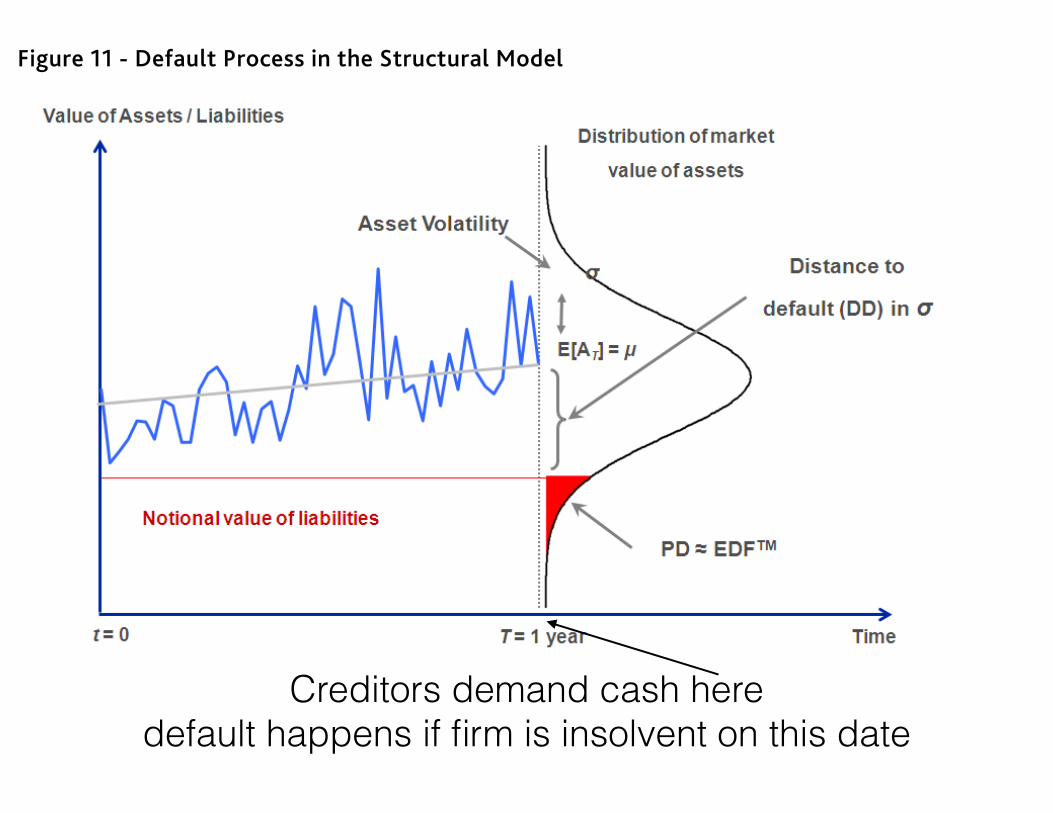
Figure 11 - Default Process in the Structural Model

The first driver is the difference between the market value of the firm’s assets and the book value of its liabilities at a future point in time.22 In Figure 11, the future point in time equates to a one-year horizon (T=1); the expected mean level of the market value of assets is the grey line, and the book value of liabilities is the red line. The differential between the assets and liabilities is a measure of leverage, or financial risk, with a smaller differential equaling greater leverage, and thus more risk. The other driver is the expected asset volatility (represented by ʍ�– the blue line is just one such possible path). Asset volatility is measure of business risk.

In this way the model incorporates the components of classic credit analysis — business risk and financial risk — that are familiar to all practitioners. In the Public Firm model, default is assumed to occur when the market value of a firm’s assets falls below the book value of its liabilities, i.e., when it has negative net worth. The probability of this occurring is approximately equal to the shaded area in the right tail of the distribution in Figure 11. In the model the probability that the obligations will not be met is a function of the firm’s distance to default (DD), which represents the number of standard deviations that the firm’s asset value is away from the default point. DD can also be viewed as a volatility-adjusted market-based measure of leverage. DD is a crucial concept in the Public Firm model. Obviously, DD is reduced (and default risk 20 Sun (2010) 21 Merton (1974). See Crosbie and Bohn (2003) for a full description of the Public Firm model. Please also see Sellers and Arora (2004) for a description of model modifications made to account for financial institutions’ special characteristics. Most of the model description in this Appendix first appeared in Dwyer & Qu (2007).

22 The model holds the book value of liabilities constant over a one-year horizon. This assumption is relaxed when calculating EDF measures for longer terms.

A company’s stock price isn’t an assessment of its creditworthiness

The model incorporates the components of classic credit analysis —business risk and financial risk — that are familiar to all practitioners

Creditors demand cash here default happens if firm is insolvent on this date

Theory behind Merton’s DD• Key Parameters:!

• 1) Leverage adjusted for asset volatility

• 2) Timing of cash flows demanded by creditors

• Regulation should impact financial firms’ choice of 1) and 2)

• Do we see that in the data?

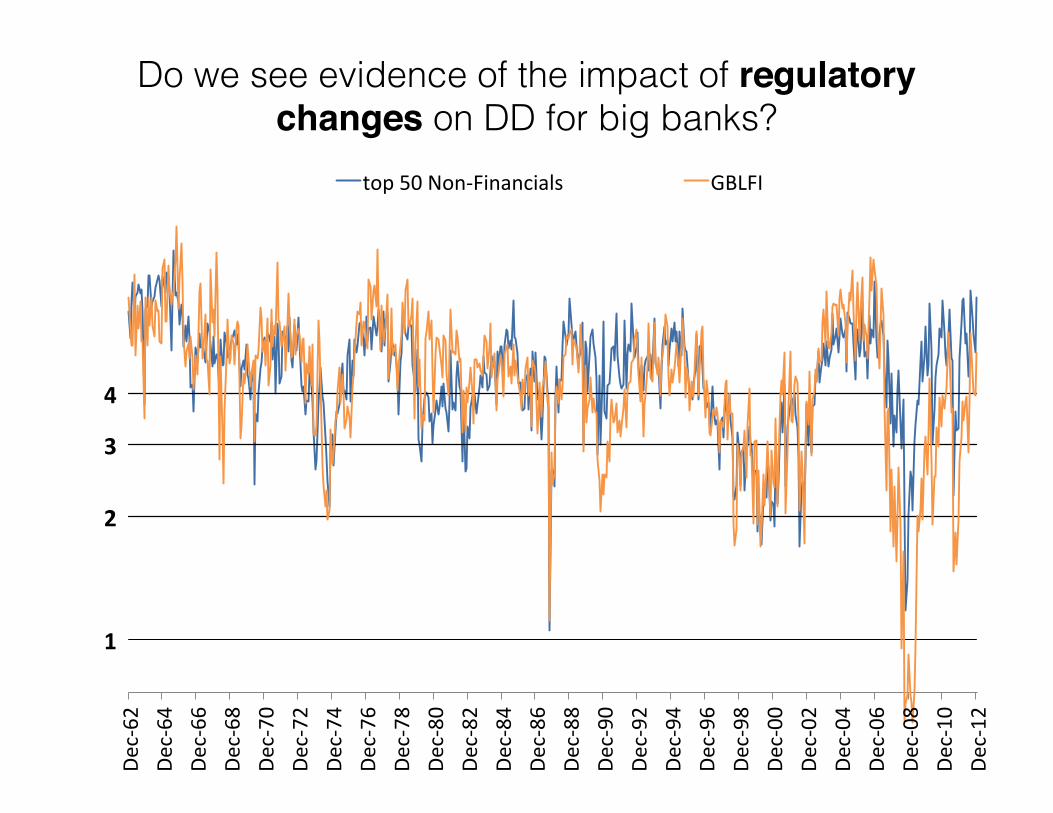
Do we see evidence of the impact of regulatory changes on DD for big banks?

1"

2"

3"

4"

Dec$62

'De

c$64

'De

c$66

'De

c$68

'De

c$70

'De

c$72

'De

c$74

'De

c$76

'De

c$78

'De

c$80

'De

c$82

'De

c$84

'De

c$86

'De

c$88

'De

c$90

'De

c$92

'De

c$94

'De

c$96

'De

c$98

'De

c$00

'De

c$02

'De

c$04

'De

c$06

'De

c$08

'De

c$10

'De

c$12

'

top'50'Non$Financials' top'50'Financials'

Figure 15: A comparison of the log median measured DI for the largest 50 financialand non-financial firms in terms of market capitalization, 1962-2012. The horizontal linesindicate the position of our benchmark cuto↵s (DI=1,2,3,4) on the log scale.

1"

2"

3"

4"

Dec$62

'De

c$64

'De

c$66

'De

c$68

'De

c$70

'De

c$72

'De

c$74

'De

c$76

'De

c$78

'De

c$80

'De

c$82

'De

c$84

'De

c$86

'De

c$88

'De

c$90

'De

c$92

'De

c$94

'De

c$96

'De

c$98

'De

c$00

'De

c$02

'De

c$04

'De

c$06

'De

c$08

'De

c$10

'De

c$12

'

top'50'Non$Financials' GBLFI'

Figure 16: A comparison of the log median measured DI for the Government Backed LargeFinancial Institutions and the largest 50 non-financial firms in terms of market capitalization,1962-2012. The horizontal lines indicate the position of our benchmark cuto↵s (DI=1,2,3,4)on the log scale.

35

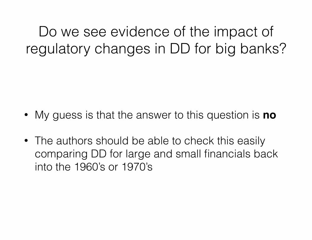
Do we see evidence of the impact of regulatory changes in DD for big banks?

• My guess is that the answer to this question is no

• The authors should be able to check this easily comparing DD for large and small financials back into the 1960’s or 1970’s

Was risked price before this crisis in the cross section? A look at Moody’s EDF by sector



EDF Metrics and Banks: The Current Situation

Negative signals for banks As we can see in Figure 5, since the credit crisis began A-rated financial institutions have exhibited higher median EDF metrics than comparably rated industrial companies. Moreover, a breakdown of median EDFs within the financial institutions space shows that for the past year banks have been the real culprits in this regard (Figure 6). As a result, the differential between banks’ median Moody’s rating and median EDF measure is quite large, when the latter is mapped to the Moody’s rating scale (Figure 7).11

Figure 5 — Median EDF Metrics for Single A Entities by Sector

0.0%

0.2%

0.4%

0.6%

0.8%

1.0%

1.2%

Jan-06 May-06 Sep-06 Jan-07 May-07 Sep-07 Jan-08 May-08 Sep-08 Jan-09 May-09 Sep-09 Jan-10 May-10 Sep-10

EDF

Date

Financials (129) Utilities (27) Corporates (205)

Figure 6 — Median EDFs for Financial Institutions Sub-groups

0.0%

0.5%

1.0%

1.5%

2.0%

2.5%

3.0%

3.5%

4.0%

Jan-07 Apr-07 Jul-07 Oct-07 Jan-08 Apr-08 Jul-08 Oct-08 Jan-09 Apr-09 Jul-09 Oct-09 Jan-10 Apr-10 Jul-10 Oct-10

EDF

Date

Banks Investment Management Insurance Findance -Other REIT

11 The mapping from EDF measures to implied ratings is determined by median EDF measures of firms in rating classes using Moody’s KMV “spot median” methodology. After calculating median EDF measures, the EDF range within a grade is computed from the median EDF of two adjacent rating grades. Once we have the EDF ranges for each category, we are able to assign an equity-implied rating for each EDF value.

EDF does not vary across types of firms pre crisis

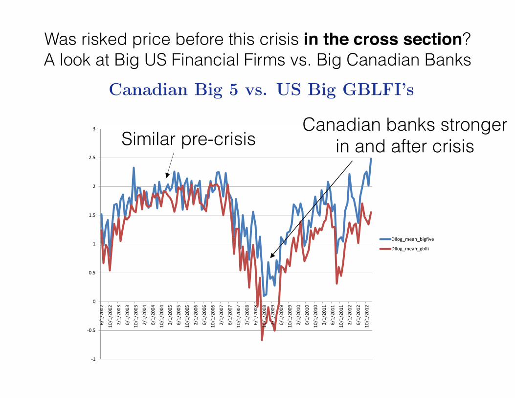
Was risked price before this crisis in the cross section? A look at Big US Financial Firms vs. Big Canadian Banks

Canadian Big 5 vs. US Big GBLFI’s

-1

-0.5

0

0.5

1

1.5

2

2.5

3

6/1/2002

10/1/200

2

2/1/2003

6/1/2003

10/1/200

3

2/1/2004

6/1/2004

10/1/200

4

2/1/2005

6/1/2005

10/1/200

5

2/1/2006

6/1/2006

10/1/200

6

2/1/2007

6/1/2007

10/1/200

7

2/1/2008

6/1/2008

10/1/200

8

2/1/2009

6/1/2009

10/1/200

9

2/1/2010

6/1/2010

10/1/201

0

2/1/2011

6/1/2011

10/1/201

1

2/1/2012

6/1/2012

10/1/201

2

DIlog_mean_bigfive

DIlog_mean_gblfi

Similar pre-crisisCanadian banks stronger

in and after crisis

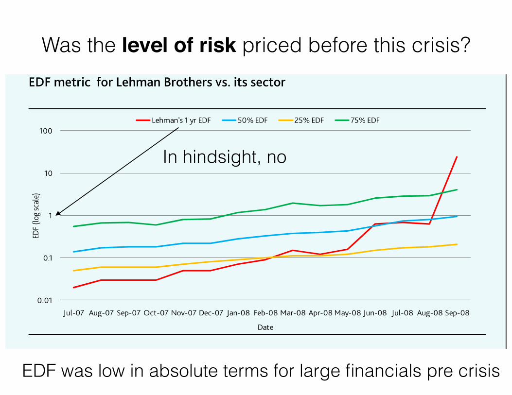
Was the level of risk priced before this crisis?



Figure 4 — Default Rates by Relative Performance (EDFs vs. Their Sectors) Bucket

0%

1%

2%

3%

4%

5%

6%

-1 -0.5 0 0.5 1 1.5 2 2.5 3 3.5 4 4.5 5

Subs

eque

nt 1

Year

Def

ault

Rate

Entity EDF Change VS. its Sector (x) Over 12 Months

We now move from an analysis of historic EDF data to the present situation, specifically to the question of why many bank EDF levels are so high, and what users can (or should) do about it.

Lehman Brothers; Lessons Learned We can draw two lessons from Lehman Brothers’ default. The first is the importance of focusing on the movement of a firm’s EDF vs. its peers. Lehman’s one-year EDF metric was 0.1% six months before the firm’s default and 0.6% three months prior to the event. These figures are low in absolute terms, of course, but represented a significant underperformance vs. the metrics for global financial institutions, as the graph below illustrates. This is consistent with the users’ tip on page 10 of tracking individual firm’s EDF measures against those of their peers, and shows the value of EDF metrics in signaling deteriorating credit situations.

Secondly, Lehman is a useful reminder that EDFs reflect information obtained from equity markets and financial statements, and that they can be no better than the quality of this information. With the benefit of hindsight we know now that the markets, regulators, and others were operating with less than complete information about Lehman’s true credit quality.

For example, the firm used certain accounting treatments to move liabilities off balance sheet on a temporary basis. As has been widely reported, Lehman sold equity and fixed income securities to a UK subsidiary and achieved “true sale” accounting treatment, even though they intended to repurchase these assets immediately after the close of their quarterly accounting dates. Inclusion of these “Repo 105 and 108” transactions into liabilities increased Lehman’s leverage ratios, since about $60 billion was concealed that otherwise would have had to go onto the balance sheet. So from an EDF model perspective, LEH’s liabilities and hence leverage were understated. Had these repos been reported correctly at June 30, 2008, the firm’s EDF metric would have been higher.

Also, in the firm’s last published financials (June 30, 2008) it reported an unencumbered liquidity pool of $35 billion - $40 billion. This was a big comfort factor for investors. The definition of unencumbered is that the assets are not pledged overnight. However, we subsequently learned that Lehman would use these assets to secure borrowings from their banks intra-day, but closed the transactions out each afternoon so that they were able to define the assets as unencumbered, (when for all practical purposes they were really pledged to the banks). Just a few days before their bankruptcy filing, the counterparty banks asked for more collateral margin from Lehman, and also asked for the pledges of the unencumbered assets to remain in force overnight. Thus, the “unencumbered asset “pool vanished. Word that the counterparties were asking for more collateral than Lehman could provide made its way out through the grapevine on the Street, hastening the company’s downfall.

EDF metric for Lehman Brothers vs. its sector

0.01

0.1

1

10

100

Jul-07 Aug-07 Sep-07 Oct-07 Nov-07 Dec-07 Jan-08 Feb-08 Mar-08 Apr-08 May-08 Jun-08 Jul-08 Aug-08 Sep-08

EDF

(log

scal

e)

Date

Lehman's 1 yr EDF 50% EDF 25% EDF 75% EDF

EDF was low in absolute terms for large financials pre crisis

In hindsight, no

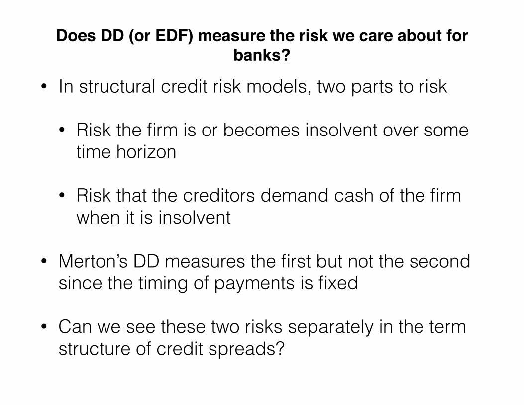
Does DD (or EDF) measure the risk we care about for banks?

• In structural credit risk models, two parts to risk

• Risk the firm is or becomes insolvent over some time horizon

• Risk that the creditors demand cash of the firm when it is insolvent

• Merton’s DD measures the first but not the second since the timing of payments is fixed

• Can we see these two risks separately in the term structure of credit spreads?

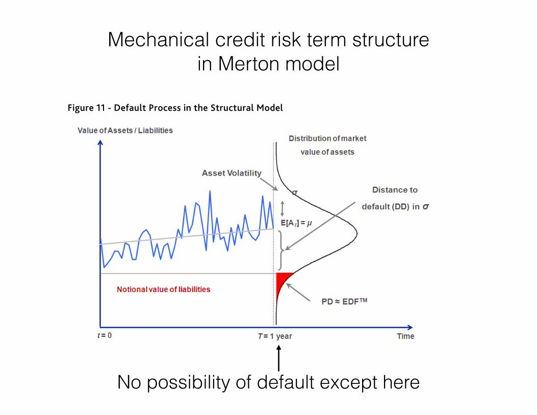
Mechanical credit risk term structure in Merton model












No possibility of default except here

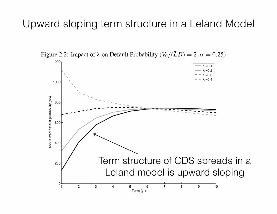
Upward sloping term structure in a Leland Model 14 CHAPTER 2. MODEL DESCRIPTION

Figure 2.2: Impact of λ on Default Probability (V0/(L̄D) = 2, σ = 0.25)

1 2 3 4 5 6 7 8 9 100

200

400

600

800

1000

1200

Term (yr)

Annu

aliz

ed d

efau

lt pr

obab

ility

(bp)

λ =0.1λ =0.2λ =0.3λ =0.4

Sensitivities to the equity price and volatility can be characterized by the CreditGrades delta, gamma andvega. As an illustration, consider a USD 1,000 notional 5-year credit default swap on a firm with a debt-per-share of USD 30 and asset specific recovery of 30 percent. The CreditGrades delta represents the sensitivityof the market value of a CDS to changes in the firm’s equity price, and can be interpreted as the number ofshares of the equity required to offset small price moves.5 Figure 2.3 shows the relationship between deltaand the equity spot price. The number of shares needed to hedge the CDS increases as spot price drops.

The CreditGrades gamma represents the change in delta with respect to spot price moves. Figure 2.4 showsthat CDS gamma increases as a stock price decreases. Further, higher levels of asset volatility dampen thevalue of gamma for default swaps on distressed credits.

Finally, the CreditGrades asset vega represents the dollar change in the CDS value per 1 percent move inasset volatility. The asset vega can be converted to an equivalent equity vega using (2.26). The relationshipbetween vega and spot price is shown in Figure 2.5. In particular, for default swaps on a credit with high stockprice, vega increases with the asset volatility, indicating the rise in downside risk with increasing uncertainty.Not surprisingly, all of the sensitivities shown in Figures 2.3 to 2.5 are quite similar to those of an equity putoption.

5In all cases here, we consider the sensitivities of the contingent leg of the CDS only, since this is where most of the sensitivityto equity lies. In other words, we assume in all cases that there is no CDS premium being paid.

Term structure of CDS spreads in a Leland model is upward sloping

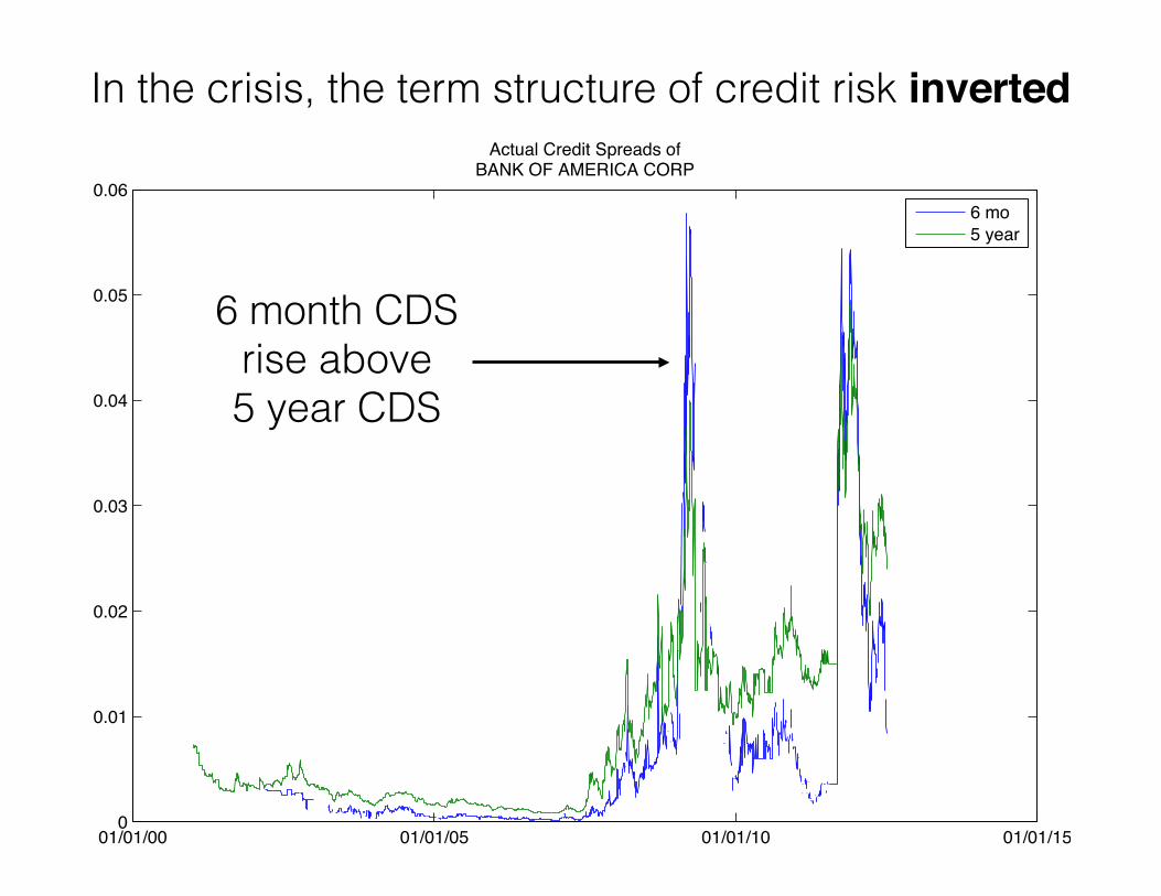
In the crisis, the term structure of credit risk inverted

01/01/00 01/01/05 01/01/10 01/01/150

0.01

0.02

0.03

0.04

0.05

0.06

Actual Credit Spreads ofBANK OF AMERICA CORP

6 mo5 year

6 month CDS rise above 5 year CDS

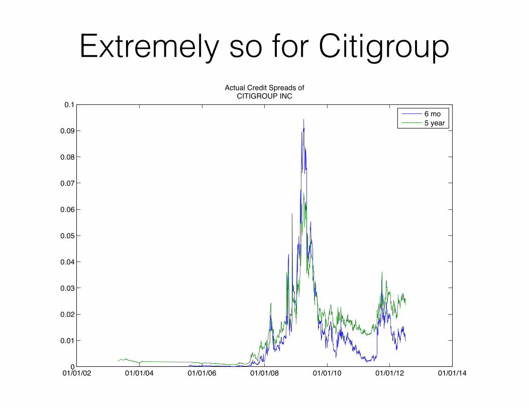
Extremely so for Citigroup

01/01/02 01/01/04 01/01/06 01/01/08 01/01/10 01/01/12 01/01/140

0.01

0.02

0.03

0.04

0.05

0.06

0.07

0.08

0.09

0.1

Actual Credit Spreads ofCITIGROUP INC

6 mo5 year

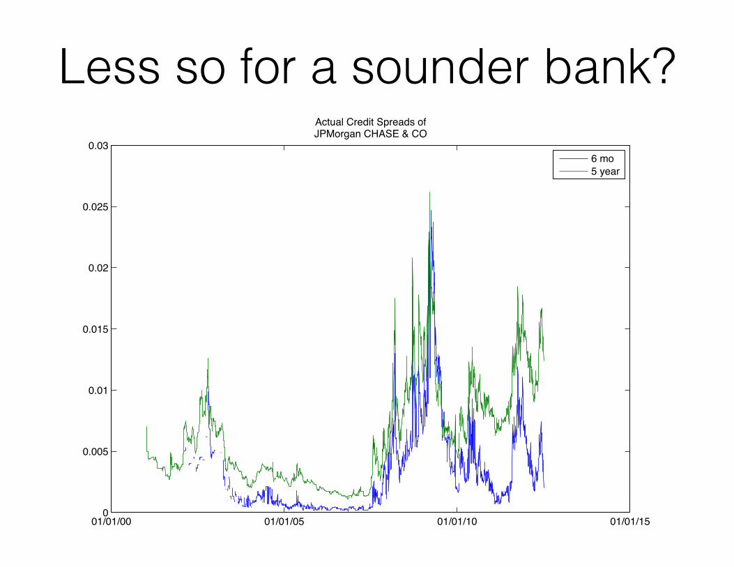
Less so for a sounder bank?

01/01/00 01/01/05 01/01/10 01/01/150

0.005

0.01

0.015

0.02

0.025

0.03

Actual Credit Spreads ofJPMorgan CHASE & CO

6 mo5 year

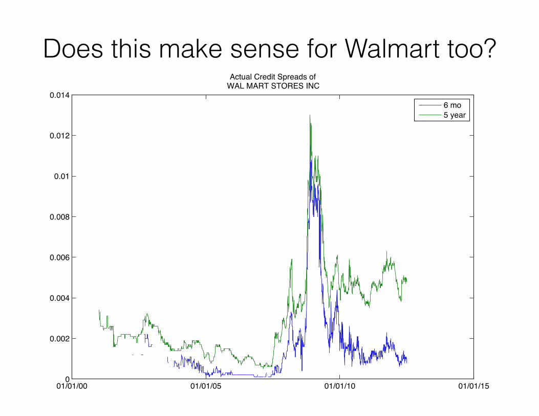
Does this make sense for Walmart too?

01/01/00 01/01/05 01/01/10 01/01/150

0.002

0.004

0.006

0.008

0.01

0.012

0.014

Actual Credit Spreads ofWAL MART STORES INC

6 mo5 year

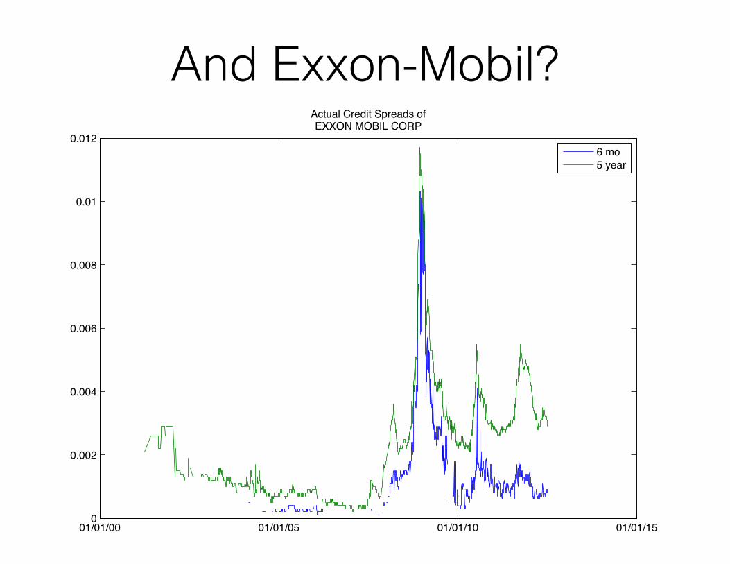
And Exxon-Mobil?

01/01/00 01/01/05 01/01/10 01/01/150

0.002

0.004

0.006

0.008

0.01

0.012

Actual Credit Spreads ofEXXON MOBIL CORP

6 mo5 year

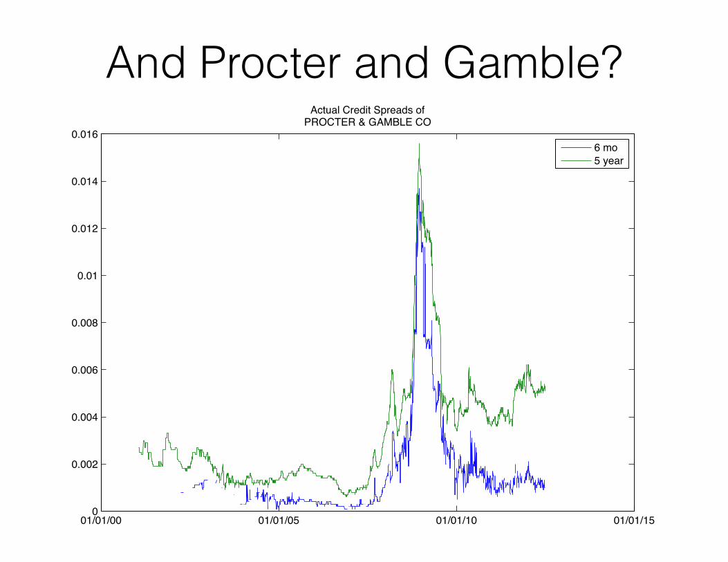
And Procter and Gamble?

01/01/00 01/01/05 01/01/10 01/01/150

0.002

0.004

0.006

0.008

0.01

0.012

0.014

0.016

Actual Credit Spreads ofPROCTER & GAMBLE CO

6 mo5 year

What was the risk? • Whatever happened in the crisis, it raised near term credit

spreads to very high levels for lots of firms.

• See the same phenomenon in short-term lending rates during the crisis

• Merton Model does not capture this risk

• Might call this “liquidity risk”

• Risk of a sudden demand for a large amount of cash when a firm is insolvent

• Is the short term credit spread a measure of this risk?

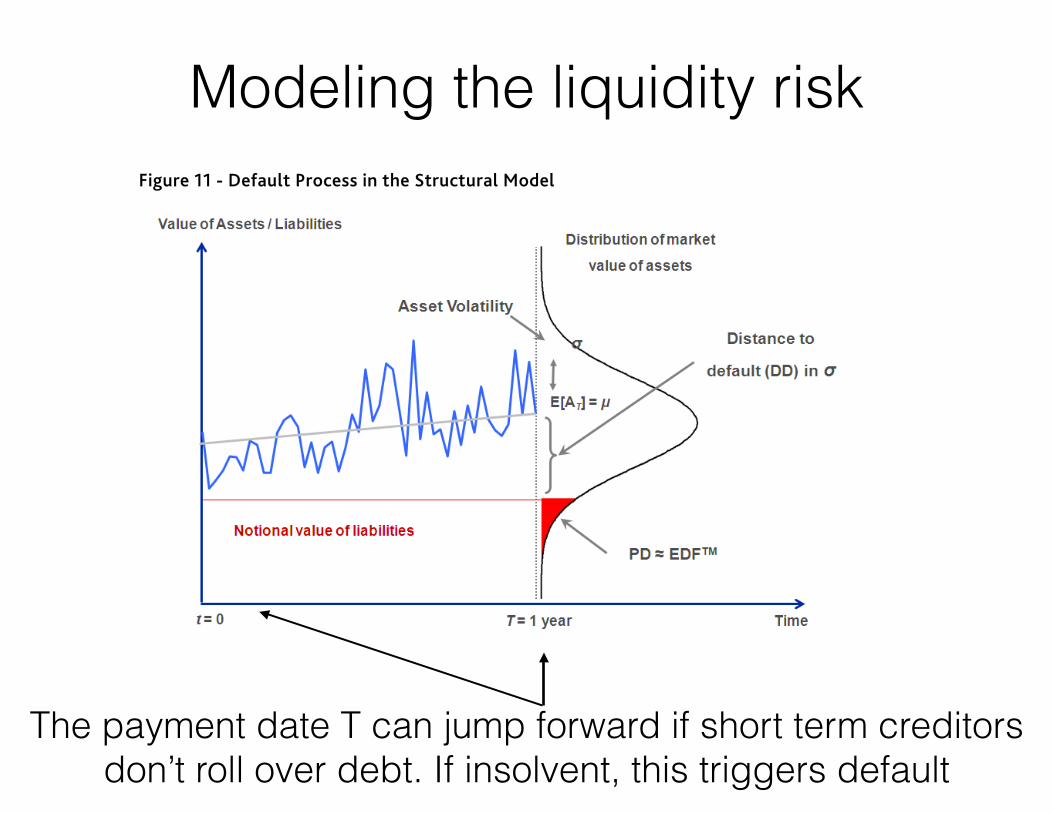
Modeling the liquidity risk












The payment date T can jump forward if short term creditors don’t roll over debt. If insolvent, this triggers default

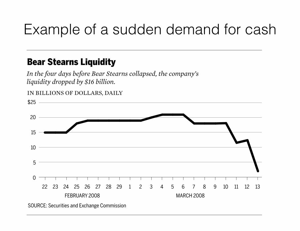
Example of a sudden demand for cash

Bear Stearns Liquidity

IN BILLIONS OF DOLLARS, DAILY

0

10

5

15

20

$25

22 23 24 25 26 27 28 29 1 2 3 4 5 6 7 8 9 10 11 12 13

SOURCE: Securities and Exchange Commission

FEBRUARY 2008 MARCH 2008

In the four days before Bear Stearns collapsed, the company’s liquidity dropped by $16 billion.

Figure .

M A R C H : T H E FA L L O F B E A R S T E A R N S

“THE GOVERNMENT WOULD NOT PERMIT A HIGHER NUMBER”

On Thursday evening, March , Bear Stearns informed the SEC that it would be“unable to operate normally on Friday.” CEO Alan Schwartz called JP Morgan CEOJamie Dimon to request a billion credit line. Dimon turned him down, citing,according to Schwartz, JP Morgan’s own significant exposure to the mortgage mar-ket. Because Bear also had a large, illiquid portfolio of mortgage assets, JP Morganwould not render assistance without government support. Schwartz spoke with Gei-thner again. Schwartz insisted Bear’s problem was liquidity, not insufficient capital. Aseries of calls between Schwartz, Dimon, Geithner, and Treasury Secretary HenryPaulson followed. To address Bear’s liquidity needs, the New York Fed made a .billion loan to Bear Stearns through JP Morgan on the morning of Friday, March .Standard & Poor’s lowered Bear’s rating three levels to BBB. Moody’s and Fitch alsodowngraded the company. By the end of the day, Bear was out of cash. Its stockplummeted , closing below .

The markets evidently viewed the loan as a sign of terminal weakness. Aftermarkets closed on Friday, Paulson and Geithner informed Bear CEO Schwartz thatthe Fed loan to JP Morgan would not be available after the weekend. Without thatloan, Bear could not conduct business. In fact, Bear Stearns had to find a buyer be-fore the Asian markets opened Sunday night or the game would be over. Schwartz,

Measuring the TBTF Subsidy• a pricing versus an engineering approach

• pricing: how much firms would have to pay for funding without the TBTF policy under current market arrangements

• a measure of the subsidy to each firm

• this paper is an example of a pricing approach

• engineering: how much would it cost firms in the aggregate to implement safer market arrangements?

• Get different answers if their are spillovers in risk

An Engineering Approach to measuring the TBTF subsidy

• How much capital and long term debt do TBTF firms need to for the system as a whole to have to have stable funding?

• Is the cost gap between their current (or pre-crisis) funding model and a safe (immune to runs) funding model the subsidy afforded by TBTF policies?

• Can we measure this funding cost gap?

Documents

Discussion of “The End of Market Discipline” Acharya