Discretionary-Accruals Models and Audit Qualifications

8/4/2019 Discretionary-Accruals Models and Audit Qualifications

http://slidepdf.com/reader/full/discretionary-accruals-models-and-audit-qualifications 1/41

1

Discretionary-Accruals Models and Audit Qualifications

Eli Bartov

Leonard N. Stern School of Business

New York University

40 W. 4th St., Suite 423

New York, NY 10012

EMAIL: [email protected]

Ferdinand A. Guland

Judy S.L. Tsui

Department of Accountancy

City University of Hong Kong

83 Tat Chee Avenue

Kowloon Tong

Hong Kong

January 2000

First draft: October 1998

This paper has been presented at Penn State, the University of Rochester, and the Ninth AnnualConference on Financial Economics and Accounting.



2

Discretionary-Accruals Models and Audit Qualifications

1. Introduction

A major strand of the earnings management literature examines managers’ use of

discretionary accruals to shift reported income among fiscal periods. Such an examination

entails specification of a model to estimate discretionary accruals. The models range from the

simple, in which total accruals are used as a measure of discretionary accruals to the relatively

sophisticated (regression), which decompose accruals into discretionary and nondiscretionary

components. The most popular six models are the DeAngelo (1986) Model, Healy (1985)

Model, the Jones (1991) Model, the Modified Jones Model (Dechow, Sloan, and Sweeney 1995),

the Industry Model (Dechow, Sloan, and Sweeney 1995), and the Cross-Sectional Jones Model

(DeFond and Jiambalvo 1994).

Dechow, Sloan, and Sweeney (1995) evaluated the relative performance of five of these

models in detecting earnings management by comparing the specification and power of

commonly used tests across discretionary accruals generated by the models. They evaluated the

specification of the test statistics by examining the frequency with which the statistics generate

type I errors and the power of the tests by examining the frequency with which the statistics

generate type II errors. Using various samples and assumptions, they demonstrated that all

models appear well specified for random samples, generate tests of low power for earnings

management, and reject the null hypothesis of no earnings management at rates exceeding the

specified test-levels when applied to samples of firms with extreme financial performance.

Additionally, they showed that the Modified Jones Model provides the most powerful test of

earnings management.



3

Prior studies have also focused on evaluating the ability of discretionary-accruals models

to segregate earnings into discretionary and nondiscretionary components by examining their

time-series properties (Hansen 1996). Other studies (e.g., Chaney, Jeter, and Lewis 1995, and

Subramanyam 1996) have used the association between stock returns, and discretionary accruals

and nondiscretionary earnings to study the valuation relevance of discretionary accruals. These

studies concluded that managers use discretionary accruals to convey their private information to

investors.

Guay, Kothari, and Watts (1996) pointed out that comparisons of discretionary-accruals

models in Dechow, Sloan, and Sweeney (1995) critically hinge on such important (implicit)

assumptions as the behavior of earnings absent discretion and how management exercises

discretion over accruals conditional on nondiscretionary earnings. Evaluations of discretionary-

accruals models using stock returns depend, additionally, on assumptions about the relation

between accounting numbers and stock prices (e.g., market efficiency with respect to earnings

information, and stock prices lead earnings). Guay, Kothari, and Watts also pointed out that

attempts to increase statistical power by using non-random samples (e.g., firms with extreme

financial performance, Dechow, Sloan, and Sweeney 1995) cloud the findings, as they increase

the likelihood that correlated omitted variables cause the results.

In an effort to improve on the methodology of this prior research for evaluating

discretionary-accruals models, Guay, Kothari, and Watts first made predictions on the basis of

explicit assumptions regarding the relation between stock returns, and discretionary accruals and

nondiscretionary earnings. Using a random sample, they then investigated whether the various

accrual-based models produce discretionary accruals and nondiscretionary earnings that conform

to their predictions. Their findings cast doubts on the ability of the models to separate accruals



4

into discretionary and nondiscretionary components. Healy (1996), however, pointed out that

Guay, Kothari, and Watts’ study relies on strong assumptions such as strong-form stock market

efficiency, and that its tests examine the aggregate relation between stock returns, discretionary

accruals, and nondiscretionary earnings, rather than relations for a specific sample where

earnings management is expected. Thus, whether these discretionary-accruals models are able to

separate accruals into discretionary and nondiscretionary components and thereby detect

earnings management is still an open empirical question.

The primary goal of this study is to evaluate empirically the ability of the cross-sectional

version of two discretionary-accruals model, the Cross-Sectional Jones Model and the Cross-

Sectional Modified Jones Model, to detect earnings management vis-à-vis their time series

counterparts. We are motivated to undertake this evaluation because the two cross-sectional

models have not been evaluated by prior research, and because, ex ante, it is unclear which type

of model dominates as each type relies on a different set of assumptions and it is an empirical

question which set is more descriptively valid. We note that the cross-sectional models have a

number of advantages over their time-series counterparts. Specifically, using a cross-sectional

rather than a time-series model in estimating discretionary accruals (e.g., the Cross-Sectional

Modified Jones Model rather than the Modified Jones Model) should result in a larger sample

size that is less subject to a survivorship bias. Moreover, cross-sectional models also allow

investigation of firms with a shorter history than required for time-series models, e.g., new

startups engaging in initial public offerings.

To allow comparisons between the ability of these two cross-sectional models and the

five models examined by prior research to detect earnings management, we also reexamine these

five models using our new sample and new research method that controls potential research



5

confounds. This reexamination will also enable us to assess the robustness of Dechow, Sloan,

and Sweeney’s (1995) findings, which seems warranted in light of the criticisms raised in the

Guay, Kothari, and Watts’ (1996) study.

One aspect of our method for evaluating the relative performance of the various models

concerns maximizing statistical power by examining the association between discretionary

accruals they generate and the likelihood of receiving an audit qualification. The intuition

underlying this approach is straightforward. It follows from prior earnings management studies

(see, e.g., Healy 1985, DeAngelo 1986, and Jones 1991) that high discretionary accruals indicate

earnings manipulations. Thus, if discretionary accruals indicate earnings manipulations, they

should be associated with the likelihood of auditors’ issuing qualified audit reports.

A distinguishing feature of our research method is our simultaneous effort to maximize

power (by carefully selecting a sample where earnings management is expected) while

minimizing potential biases arising from using a non-random sample that may lead to erroneous

inferences (by adding controls for potential research confounds). For example, Dechow, Sloan,

and Sweeney (1995, 208-209) reported that for firms experiencing extreme financial

performance, the discretionary-accruals models they evaluate are unable to completely extract

the low (high) non-discretionary accruals associated with the low (high) earnings performance.

We thus evaluate the association between discretionary accruals and audit qualifications after

controlling for earnings performance.

Chi-square tests and univariate logistic-regression tests of 166 distinct firms with

qualified audit opinions and 166 matched-pair firms with clean reports show that all models,

except the DeAngelo Model, are successful in detecting earnings management. More

specifically, the chi-square tests show a relatively high number of firms with a clean opinion in



6

the lowest discretionary accruals quintile and a relatively high number of firms with a qualified

report in the highest discretionary accruals quintile. The univariate logistic regressions also

show a significant relation between discretionary accruals and the likelihood of receiving

qualified reports. Thus, like Dechow, Sloan, and Sweeney (1995), using univariate tests that do

not control for potential research confounds, we provide evidence suggesting that the Jones

Model, the Modified Jones, the Healy Model, and the Industry Model are able to detect earnings

management. However, with respect to the DeAngelo Model, their findings differ from ours.

While they conclude that this model is also successful in detecting earnings management, our

findings do not support the ability of the DeAngelo Model to detect earnings management.

While our matched-pair design alleviates concerns regarding the role of potential

research confounds, it does not eliminate them entirely as the control firms differ from the test

firms with respect to certain firm characteristics. In an effort to assess the effect of potential

research confounds on our findings, we replicate the logistic regression tests after augmenting

the model with explanatory variables capturing auditors' litigation risk (Lys and Watts 1994) as

well as extreme earnings performance (Dechow, Sloan, and Sweeney 1995). The results show

that only the two cross-sectional models continue to perform well. The Jones Model, the

Modified-Jones Model, the Healy Model and the Industry Model are no longer able to

distinguish between firms with clean and qualified audit reports. The results also indicate that

two of the proxies for litigation risk (book-to-market ratios and financial leverage) as well as the

earnings performance variable are important control variables for studying discretionary

accruals.



7

The primary contribution of this study lies in our finding that the Cross-Sectional Jones

Model and the Cross-Sectional Modified Jones Model, not evaluated by prior research, perform

better than their time-series counterparts in detecting earnings management. This result is

important for future earnings management research particularly because using a cross-sectional

model, rather than its time-series counterpart, should result in a larger sample size that is less

subject to a survivorship bias. It will also allow examining samples of firms with short history.

Another contribution of this study is that our findings from the multiple logistic regressions

demonstrate the importance of controlling for research confounds in earnings management

studies and identify three important control variables: book-to-market ratios, financial leverage,

and earnings performance.

The next section describes the seven competing discretionary-accruals models we

evaluate and outlines the theoretical background underlying our investigation. Section 3 reports

the sample selection procedure and describes the data. Section 4 outlines the tests and discusses

the results, and the final section concludes the study.

2. Theoretical background

2.1 DISCRETIONARY-ACCRUALS MODELS

The seven competing discretionary-accruals models considered in this study are

described below.

The DeAngelo Model

The DeAngelo (1986) Model uses the last period’s total accruals (TAt - 1) scaled by

lagged total assets (At-2) as the measure of nondiscretionary accruals. Thus, the model for



8

nondiscretionary accruals (NDAt) is:

NDAt = TAt - 1 / At - 2 (1)

The discretionary portion of accruals is the difference between total accruals in the event year t

scaled by At-1 and NDAt.

The Healy Model

The Healy (1985) Model uses the mean of total accruals (TA τ) scaled by lagged total

assets (A τ-1) from the estimation period as the measure of nondiscretionary accruals. Thus, the

model for nondiscretionary accruals in the event year t (NDAt) is:

NDAt = 1/n Σ τ(TA τ / A τ-1 ) (2)

where:

NDAt is nondiscretionary accruals in year t scaled by lagged total assets;

n is the number of years in the estimation period; and

τ is a year subscript for years (t-n, t-n+1,…,t-1) included in the estimation period.

The discretionary portion of accruals is the difference between total accruals in the event

year t scaled by At-1 and NDAt. While the DeAngelo Model, in which the estimation period for

nondiscretionary accruals is restricted to the previous year’s observation, may appear a special

case of the Healy (1985) Model, the two models are quite different. While underlying the

DeAngelo Model is the assumption that NDA follow a random walk process, the Healy Model

assumes that NDA follow a mean reverting process.



9

The Jones Model

Jones (1991) proposes a model that attempts to control for the effects of changes in a

firm’s economic circumstances on nondiscretionary accruals. The Jones Model for

nondiscretionary accruals in the event year is:

NDAt = α1(1 / At - 1) + α2(∆REVt / At - 1) + α3(PPEt / At - 1 ) (3)

where:

NDAt is nondiscretionary accruals in year t scaled by lagged total assets;

∆REVt is revenues in year t less revenues in year t - 1;

PPEt is gross property plant and equipment at the end of year t ;

At - 1 is total assets at the end of year t - 1; and

α1, α2, α3 are firm-specific parameters.

Estimates of the firm-specific parameters, α1, α 2, and α3, are obtained by using the

following model in the estimation period:

TAt / At - 1 = a1(1/At - 1) + a2(∆REVt / At - 1) + a3(PPEt / At - 1) + εt (4)

where:

a1, a2, and a3 denote the OLS estimates of α1, α2, and α3, and TAt is total accruals in year t . εt is

the residual, which represents the firm-specific discretionary portion of total accruals. Other

variables are as in equation (3).

The Modified Jones Model

The Modified Jones Model is designed to eliminate the conjectured tendency of the Jones

Model to measure discretionary accruals with error when discretion is exercised over revenue



10

recognition. In the modified model, nondiscretionary accruals are estimated during the event

year (i.e., the year in which earnings management is hypothesized) as:

NDAt = α1(1/At - 1) + α2[(∆REVt - ∆RECt) / At - 1]+ α3(PPEt / At - 1) (5)

where:

∆RECt is net receivables in year t less net receivables in year t - 1, and the other variables are as

in equation (3). It is important to note that the estimates of α1, α2, α3 are those obtained from the

original Jones Model, not from the modified model. The only adjustment relative to the original

Jones Model is that the change in revenues is adjusted for the change in receivables in the event

year (i.e., in the year earnings management is hypothesized).1

The Industry Model

The Industry Model also relaxes the assumption that nondiscretionary accruals are

constant over time. Instead of attempting to model the determinants of nondiscretionary accruals

directly, the Industry Model assumes that the variation in the determinants of nondiscretionary

accruals are common across firms in the same industry. The Industry Model for

nondiscretionary accruals is:

NDAt = β1 + β2median j(TAt / At - 1) (6)

where:

NDAt is as in equation (3), and median j(TAt / At - 1) is the median value of total accruals in year t

scaled by lagged total assets for all non-sample firms in the same two-digit standard industrial

1This approach follows from the assumption (underlying all discretionary-accrual models) that during the

estimation period, there is no systematic earnings management.



11

classification (SIC) industry (industry j) . The firm-specific parameters β1 and β2 are estimated

using OLS on the observations in the estimation period.

The Industry Model, the Healy Model, and the Jones Model are estimated over an eight-

year period ending just prior to the event year.2

For example, discretionary accruals for the first

sample year 1980 are computed on the basis of models estimated over the eight-year period,

1972 - 1979, discretionary accruals for the second sample year, 1981, are computed on the basis

of models estimated over the period 1973 - 1980, etc. This choice of estimation period, which is

comparable to prior research (see, e.g., Dechow, Sloan, and Sweeney 1995, 203), represents a

tradeoff. While using long time series of observations improves estimation efficiency, it also

leads to a smaller sample size and increases the likelihood of a structural change occurring

during the estimation period.

Cross-Sectional Models

The two cross-sectional models this study is first to examine are the Cross-Sectional

Jones Model and the Cross-Sectional Modified Jones Model. These two models are similar to

the Jones and Modified Jones models, respectively, except that the parameters of the models are

estimated by using cross-sectional, not time-series, data (see, e.g., DeFond and Jiambalvo 1994).

Thus, the parameter estimates, α1, α2, and α3, of equation (3) are industry and year specific

rather than firm specific, and are obtained by estimating equation (4) using data from all firms

matched on year (i.e., the event year) and two-digit SIC industry groupings.

We note that each type of model relies on a different set of assumptions that are unlikely

2 Note that the Modified Jones Model’s parameter estimates are obtained from the Jones Model.



12

to hold for all firms. The choice between the time-series version and the cross-sectional version

of the Jones Model thus represents tradeoffs, and it is an empirical question which choice is

preferable. For example, while an assumption underlying the time-series version is that the

length of a firm’s operating cycle does not change over the estimation period and the event year,

underlying the cross-sectional version is an assumption that all firms in the same industry have a

similar operating cycle. Indeed, in reality both assumptions are unlikely to hold for all firms.

Still, if our sample consists primarily of mature firms, the changes overtime should not be

significant. And if our sample firms are not much different from the average firm in their

industry, the fact that the cross-sectional version forces the coefficients to be the same for all

firms in the industry should not represent a serious problem. Should, however, the discretionary

accruals generated by the models reflect primarily these limitations, not the component of

earnings manipulated by management, we would not expect to find systematic differences in

discretionary accruals between test and control samples appropriately matched, as these

limitations should have a similar effect on both samples.

Total Accruals

The empirical estimation of all seven models involves computing total accruals (TA).

Along the lines of prior research (e.g., Healy 1985, and Jones 1991), we use the balance sheet

approach to compute TA as follows:

TAt = ∆CAt - ∆Casht - ∆CLt + ∆DCLt - DEPt (7)

where:

∆CAt is the change in current assets in year t (Compustat data # 4);

∆Casht is the change in cash and cash equivalents in year t (Compustat data # 1);



13

∆CLt is the change in current liabilities in year t (Compustat data # 5);

∆DCLt is the change in debt included in current liabilities in year t (Compustat data # 34); and

DEPt is depreciation and amortization expense in year t (Compustat data # 14).

Collins and Hribar (1999) argued that using this balance sheet approach to compute total

accruals is inferior in certain circumstances to a cash-flows-statement based approach. Because

statement-of-cash-flows data are available only from 1987 and because the time-series models

we evaluate require nine years of data, we are unable to measure accruals using the statement of

cash flows. Still, we can report that the rank correlation between our measure of total accruals

and that based on the statement of cash flows--for a small subset of firms for which cash flows

data were available--was 0.96. This high correlation, which was highly statistically significant,

alleviates concerns that the balance sheet approach contaminates our tests.

2.2 DISCRETIONARY ACCRUALS AND AUDIT QUALIFICATIONS

The standard agency cost model portrays the role of the auditor as a monitoring

mechanism to reduce agency costs (see, e.g., Jensen and Meckling 1976). Agency costs include

managers’ incentives to manage earnings. Kinney and Martin (1994) reviewed nine studies and

concluded that auditing reduces positive bias in pre-audit net earnings and net assets. Hirst

(1994) also demonstrated that auditors are sensitive to earnings manipulations through both

income-increasing accruals and income-decreasing accruals, and that they are able to detect

management incentives to manipulate earnings. Tests involving the association between audit

qualifications and stock returns indicate that investors perceive qualified audit reports as

informative. Dopuch, Holthausen and Leftwich (1986), Choi and Jeter (1992), and Loudder,

Khurana and Sawyers (1992) all reported negative stock price reactions to audit qualifications.



14

Our goal is to evaluate the ability of various discretionary-accruals models to detect

earnings management by testing the association between a firm’s discretionary accruals

generated by a model and the firm’s likelihood of receiving a qualified audit report. If

discretionary accruals produced by a model indicate earnings management, then the higher the

discretionary accruals in absolute value, the higher should be the probability for a qualified audit

report. Our testing approach follows from the methods of prior earnings management research

(see, e.g., Healy 1985, DeAngelo 1986, and Jones 1991), which have relied on discretionary

accruals to detect earnings manipulations.

Still, the extent to which auditors are expected to detect earnings management depends on

the quality of the audit. DeAngelo (1981) defined audit quality as the joint probability of

detecting and reporting material financial statement errors, which will depend in part on the

auditor’s independence. Higher quality audit firms are expected to hire skilled professionals who

can develop more effective tests for detecting earnings management. Moreover, higher quality

auditors are less willing to accept questionable accounting practices and more likely to report

errors and irregularities.

Big-Six auditors are identified in the literature as higher quality auditors (see, e.g.,

Palmrose 1988, 63), as they have the technological capability in detecting earnings management,

and when detected, there is a higher probability that they will report it. Investors seem to agree

with this claim. Teoh and Wong (1993), for example, reported that earnings response

coefficients of firms audited by Big-Eight firms are higher than those of firms audited by non-

Big-Eight firms, and concluded that the market perceives financial information audited by Big-

Eight firms as more credible. This discussion leads us to perform a supplementary test that

examines qualified audit reports produced by Big-Six and non-Big-Six audit firms separately.



15

3. Data

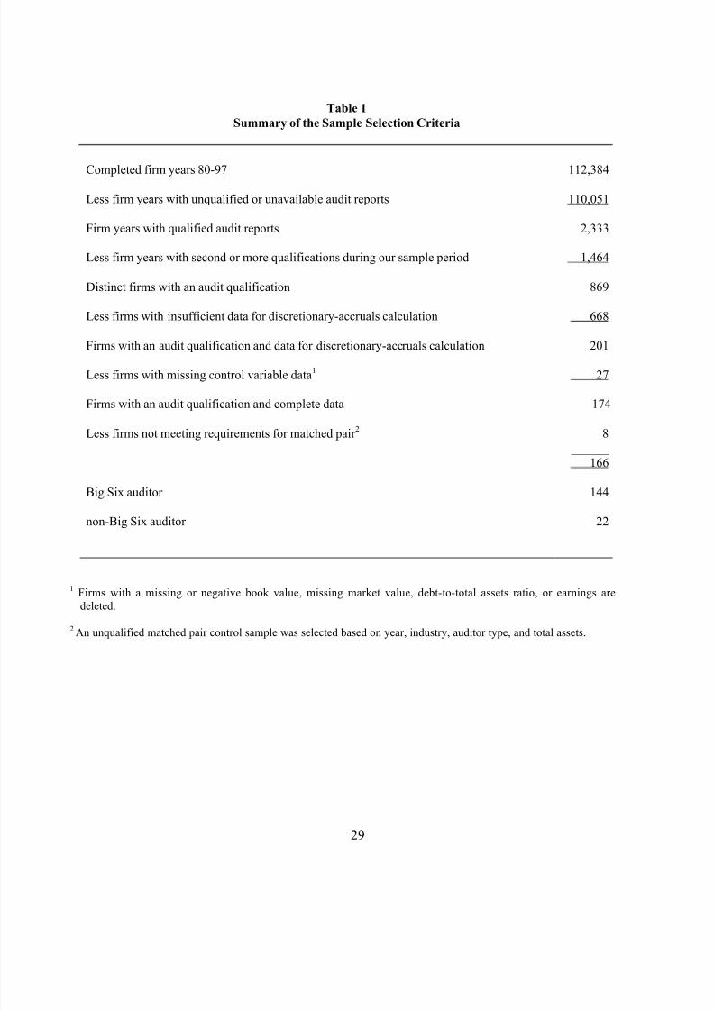
The sample selection procedure and its effects on the sample size are summarized in

Table 1. Initially, 112,384 firm-year observations for the 18-year period, 1980 – 1997, are

retrieved from the annual Compustat database. Our sample period commences in 1980 because

1972 is the first year for which the annual Compustat data are available for us, and because the

estimation of the parameters of the time-series version of the Jones Model requires eight years of

data. Next, we delete all firm years with unqualified audit reports, reducing the sample size to

2,333 firm years. We also drop 1,464 firm years with second or more audit qualifications during

our sample period, decreasing our sample size to 869 distinct firms. We then eliminate 668 firms

due to a lack of sufficient time-series data for estimating the Jones Model or for computing the

event year’s discretionary accruals for the Modified Jones Model, reducing the sample size to

201 firms. Next, we delete 27 firms with missing control-variable data required for the multiple

regression analyses, reducing the sample size to 174 firms. Finally, we delete 8 firms due to

unavailability of a matched pair, reducing the final size of the test sample to 166 distinct firms.

Discretionary accruals for the DeAngelo Model and the Healy Model are calculated as

the difference between total accruals scaled by lagged total assets in the event year and the

average of that variable in the estimation period, which is restricted to one year for the former.

We calculate the industry median discretionary accruals for each year, which is required to

estimate the Industry Model, based on two-digit SIC groupings. Thus, estimating these three

models does not represent additional data requirements.

Each firm year of the test sample is matched with a control firm with an unqualified audit

report in the event year. We select the control sample using the following four criteria: (1) fiscal



16

year, (2) two-digit SIC code, (3) auditor type (Big Six, non-Big Six), and (4) nearest total assets

amount.

Auditor’s opinion is the annual Compustat data # 149, which ranges from 0 to 5. To be

selected as our test sample, a firm has to have a qualified opinion (a value of 2), and to qualify

for our control sample, a firm has to have an unqualified opinion (a value of 1).3

The code

description defines a qualified opinion (code 2) as one in which “financial statements reflect the

effects of some limitation on the scope of the examination or some unsatisfactory presentation of

financial information.” An example of an auditor’s opinion coded as 2 by Compustat is the 1987

audit report of Boston Edison Co., issued by Coopers & Lybrand, which states “...the company

has incurred significant replacement fuel and power costs.... Such amounts have been billed to

customers but are subject to possible refund….”4

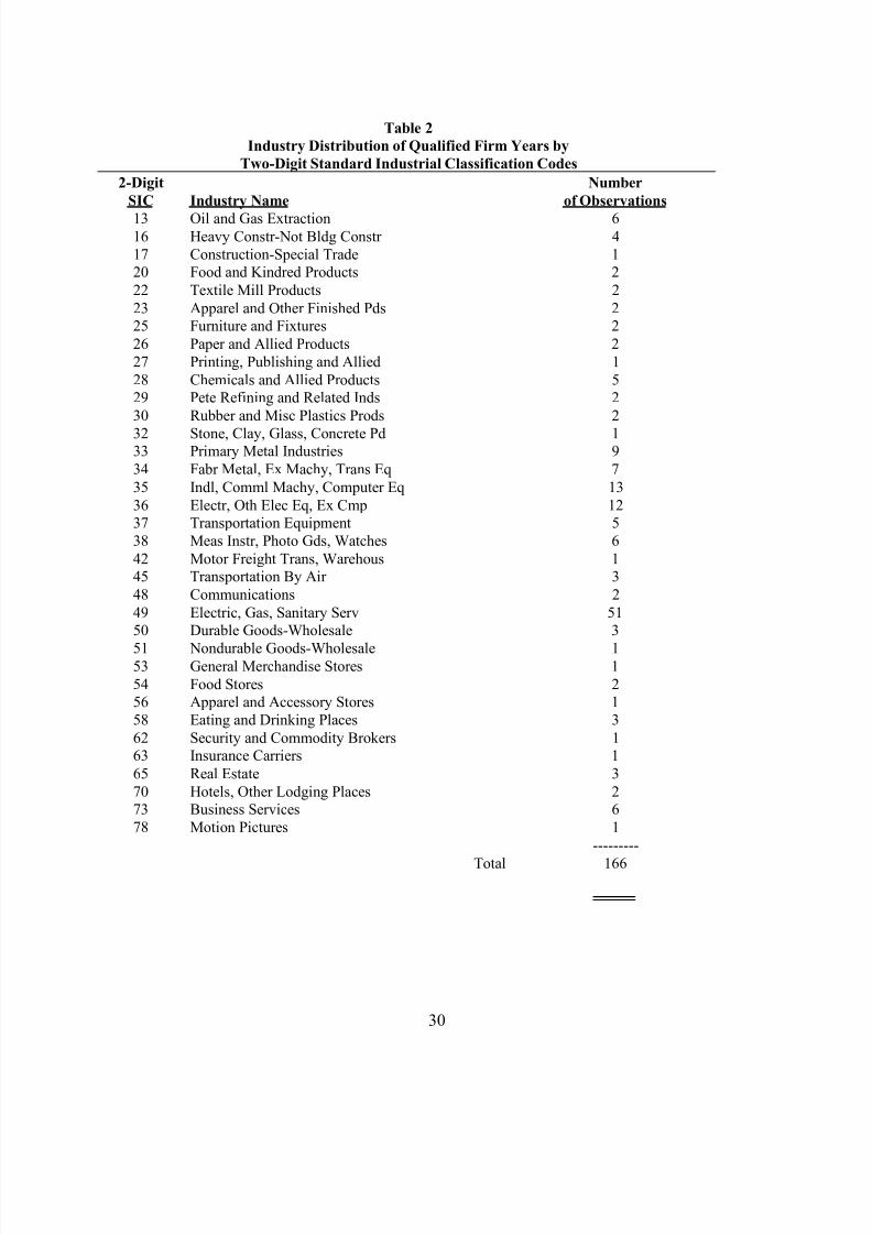
Table 2 describes the industry distribution of the qualified audit sample by two-digit SIC

codes. Our sample firm years are in 35 different two-digit standard industrial classifications.

Thus our sample contains a broad cross-section of firms. While in general there is no evidence

of industry clustering within our sample, about 30 percent of the sample firms are in the Electric,

Gas, and Sanitary Service industry (SIC 49). In the next section, we thus evaluate the effect of

the firms in this industry on our findings.

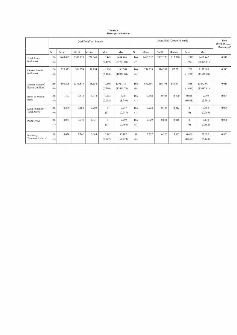
Table 3 provides descriptive statistics for the qualified-auditor-opinion test sample and

the unqualified-auditor-opinion control sample, as well as p-values of non-parametric tests for

3Codes not included in our sample are: code 0, unaudited financial statements, code 3, a going concern

qualification, code 4 unqualified opinion with explanatory language, and code 5 adverse opinion. Adverse opinions,

code 5, are not included, as they did not exist in our sample period.

4Recording revenue when important uncertainties exist is a common misapplication of accounting

principles in situations where management attempts to distort the real financial performance of a firm (see, e.g.,

Schilit 1993, pp. 1-2).



17

equality between the two samples. From reading across the table, we note two points. First, all

variables contain outlying observations, as evidenced by the minimum and maximum before

winsorization. This is to be expected when accounting data are pooled over time and across

firms. To alleviate this problem, we winsorize all variables so that the minimum and maximum

values of each variable lie within three standard deviations from its mean.5

Second, there is little

difference between the test and control firms with respect to total assets, current assets, and

inventory turnover ratio. Thus, our matching procedure is quite successful in creating a control

sample that is similar to the test sample with respect to three important firm characteristics.

These similarities alleviate concerns that differences between our test and control samples with

respect to a firm’s stage in its life cycle or the length of its operating cycle confound our tests.

Still, the procedure is not fully successful as the test and control samples are different in terms of

market capitalization, book-to-market ratios, financial leverage, which may proxy for litigation

risk (see Lys and Watts 1994), and earnings performance. In the latter part of the next section,

we thus perform multiple regression analyses that evaluate whether these differences confound

our tests.

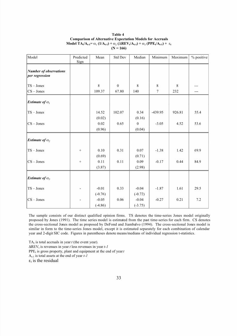
Finally, Table 4 displays a comparison between the parameter estimates generated by the

time-series version and those generated by the cross-sectional version of the Jones Model. The

results indicate that the standard deviation of all parameter estimates generated by the cross-

sectional models are substantially lower than their time-series counterparts, the number of

outliers is smaller, and the percentage of estimates with the predicted signs is greater.

Additionally, the number of observations available for estimating the model is typically much

5Winsorizing at five standard deviations left the results unchanged.



18

higher for the cross-sectional version. For example, the median number of observations for the

cross-sectional version is 140 and for the time-series version is 8. Similar findings have also

been documented by Subramanyam (1996, Table 1) notwithstanding differences in sample size

(166 vs. 21,135 firms years), time period (1980-1997 vs. 1973-1993), and sample selection

criteria (carefully selected sample vs. randomly selected sample). The similarity between the

results of the two studies alleviates concerns that our non-random sample leads to biased results

and thus elevates confidence in the validity of our findings.

4. Tests and Results

4.1 UNIVARIATE TESTS

We begin our formal assessment of the relative performance of the various discretionary-

accruals models in detecting earnings management by conducting univariate chi-square tests and

logistic regression tests that do not consider potential research confounds. For the chi-square

tests, we combine the control and test firms into one sample, and assign them to five quintiles on

the basis of the absolute value of their discretionary accruals: firms with the smallest (largest)

discretionary accruals are assigned to the first (fifth) discretionary-accruals quintile. A

discretionary-accruals model that successfully separates earnings into its components,

nondiscretionary earnings and discretionary accruals, should generate a relatively high number of

unqualified (control) firms assigned to the first quintile and a relatively high number of qualified

(test) firms assigned to the fifth quintile. As mentioned above, the intuition of this approach

follows from a maintained hypothesis underlying prior earnings management studies (see, e.g.,

Healy 1985, DeAngelo 1986, and Jones 1991) that high discretionary accruals are inevitably

coincident with earnings manipulations.



19

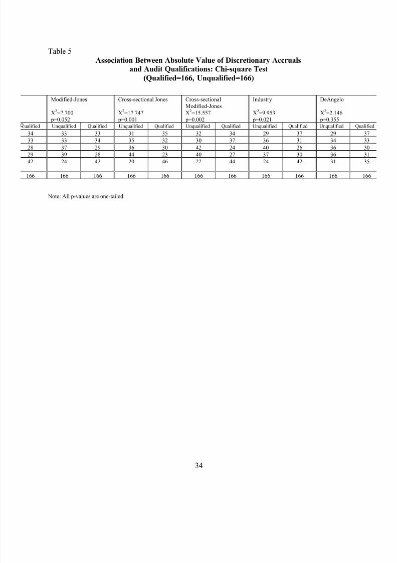
Table 5 reports the findings from the chi-square tests.6

The results are statistically

significant in the predicted direction for the two cross-sectional models, the Healy Model, and

the Industry Model, and marginally significant for the Jones Model and the Modified-Jones

Model. For example, for the Cross-Sectional Jones Model, the number of unqualified (control)

firms declines from 31 in the first (low-discretionary-accruals) quintile to 20 in the fifth (high-

discretionary-accruals) quintile, and the number of qualified (test) firms increases from 35 in the

first quintile to 46 in the fifth quintile. A chi-square test indicates that the differences between

the test and control samples are statistically significant at a 2.5 percent level. For the DeAngelo

Model, however, the numbers of control (test) firms in the lowest-discretionary-accruals quintile,

29 (37), are nearly identical to the numbers of control (test) firms in the highest quintile, 31 (35).

A chi-square test indicates that the differences between the two samples are statistically

insignificant.

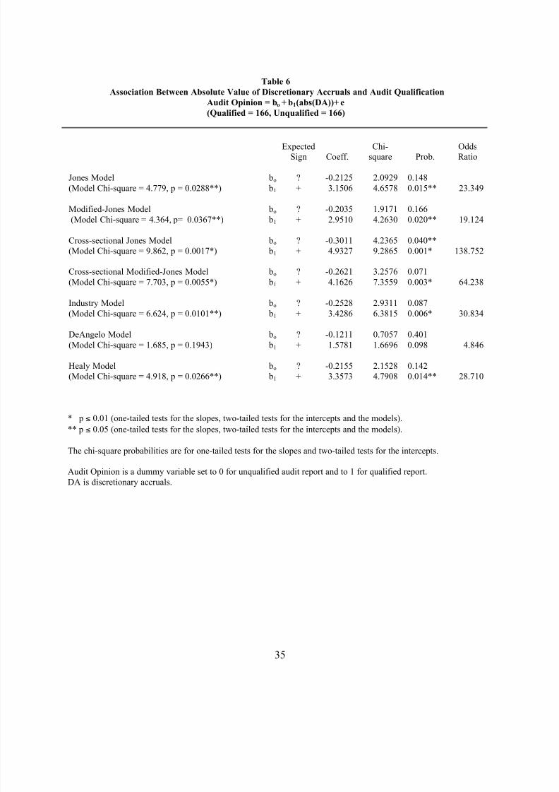
Table 6 reports the results for the logit analyses, regressing the audit opinion (a dummy

variable set to zero for an unqualified report and to one for a qualified report) on (the absolute

values of) discretionary accruals. Consistent with our chi square tests’ results, the results in

Table 6 show that all models, except the DeAngelo Model which continues to perform poorly,

yield a highly statistically significant parameter estimate in the predicted direction on the

discretionary accruals variable.

Overall, two preliminary conclusions emerge from the univariate tests. First, with the

exception of the DeAngelo Model, our results from the univariate tests, which do not consider

6Since all our predictions are directional, all tests are one-tailed.



20

potential research confounds, provide external validation for the findings in Dechow, Sloan, and

Sweeney (1995) regarding the ability of the Jones Model, the Modified-Jones Model, the Healy

Model, and the Industry Model to detect earnings management.7

Second, the performance of the two cross-sectional models is not inferior to that of their

time-series counterparts. This implies that future earnings management research should use the

cross-sectional models because the use of time-series data results in a substantially smaller

sample size and may even lead to a serious survivorship bias. The Cross-Sectional Jones Model

is the best choice as, unlike the modified model, it does not use the change-in-receivables-

variable to compute discretionary accruals in the event year and, thus, is likely to result in a

somewhat larger sample.

4.2 MULTIPLE LOGISTIC REGRESSION TESTS

Prior research has argued that accruals management studies may be plagued with a

correlated-omitted-variables problem that may bias the numbers produced by discretionary-

accruals models. While our matched-pair design alleviates this problem, this design is

unsuccessful in totally resolving it, as the match was not perfect. In an effort to further address

this problem, we perform a multiple logistic regression test that controls for book-to-market

ratios, firm size (market capitalization), financial leverage (long-term debt to-total assets ratio),

and extreme earnings performance (the absolute change in income from continuing operations in

7Our results differ from the Dechow, Sloan, and Sweeney’s (1995) results with respect to the DeAngelo

Model. They (p. 223) ranked the DeAngelo Model last in terms of its ability to detect earnings management, but

concluded that it is able to detect earnings management. Our results also show that the DeAngelo Model exhibited

the worst performance, but cast doubts on the ability of this model to detect earnings management.





22

on the extreme earnings performance variable is expected to be positive for two reasons. First,

results in Dechow, Sloan and Sweeney (1995, Table 3) imply that discretionary-accruals models

produce low (high) discretionary accruals for firm-years with low (high) earnings because they

fail to completely extract the non-discretionary accruals of firms experiencing extreme earnings

performance. Second, other things being equal, auditors may be more likely to issue qualified

reports for firms with extreme earnings, perhaps to mitigate litigation risk.

A problem may arise, however, from adding these explanatory variables to the

regressions, as they contain outlying observations (see Table 3 above). As before, we address

this problem by winsorizing all explanatory variables at three standard deviations.

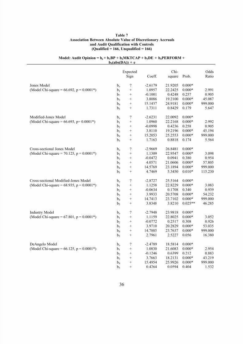
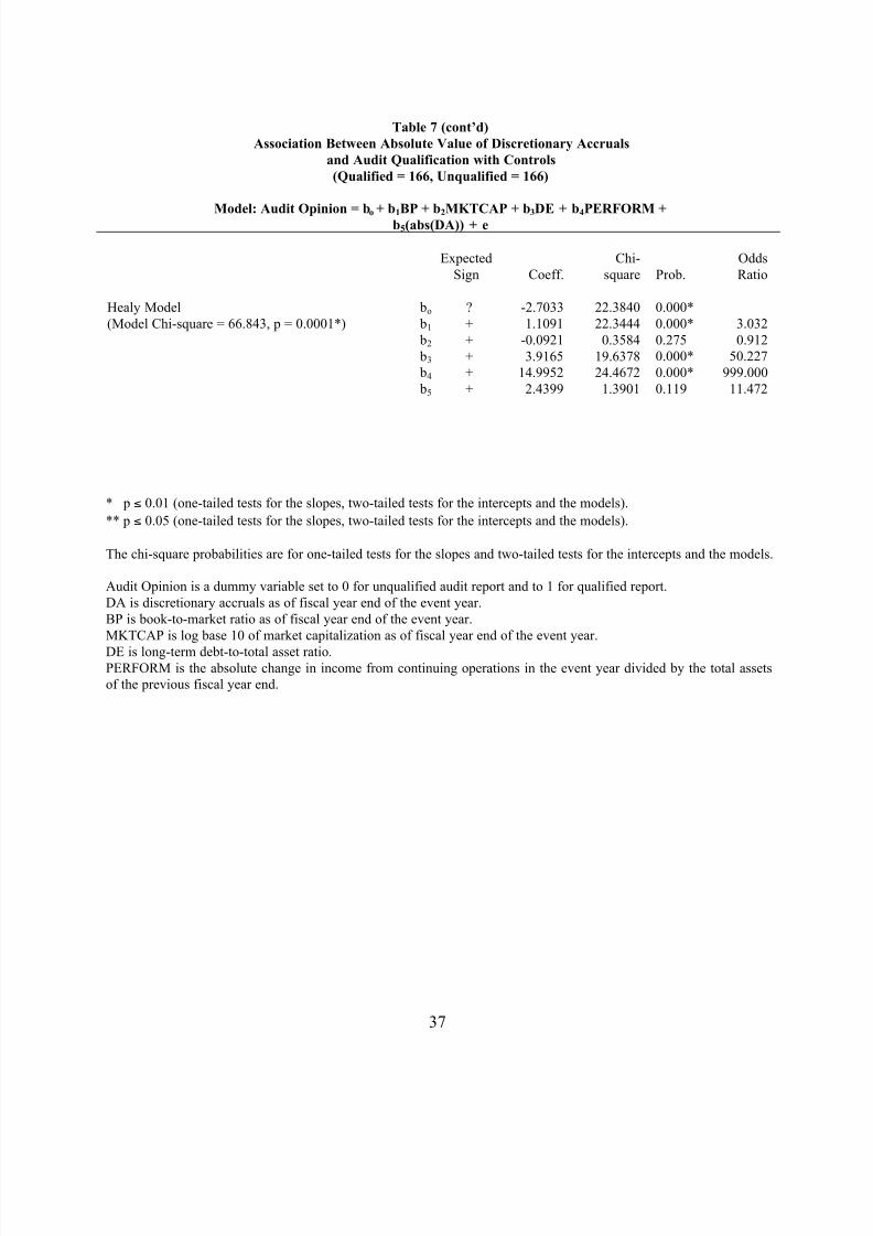
Table 7 reports the results of the logistic regressions, regressing the audit opinion (a

dummy variable set to zero for an unqualified report and to one for a qualified report) on (the

absolute values of) discretionary accruals and the four control variables. There are two points to

notice. First, only the Cross-Sectional Jones Model and the Cross-Sectional Modified Jones

Model successfully distinguish between firms with qualified audit reports and firms with

unqualified reports. For these two models, the parameter estimates on the discretionary accruals

variable are positive and highly statistically significant. In contrast, the Jones Model, the

Modified-Jones Model, the Industry Model, the DeAngelo Model, and the Healy Model fail to

generate significant results.9 These results demonstrate the superiority of the cross-sectional

models vis-à-vis their time-series counterparts and thus reinforce our conclusion that future

accruals management research should use the former rather than the latter. Second, three of the

9We further assess the sensitivity of our results by adding to the logistic regression a variable capturing past

earnings performance. The results, not reported for parsimony, are unchanged.



23

four control variables, book-to-market ratios, financial leverage, and earnings performance are

significant in all models. This finding highlights the importance of controlling for these three

variables in accruals management studies.10

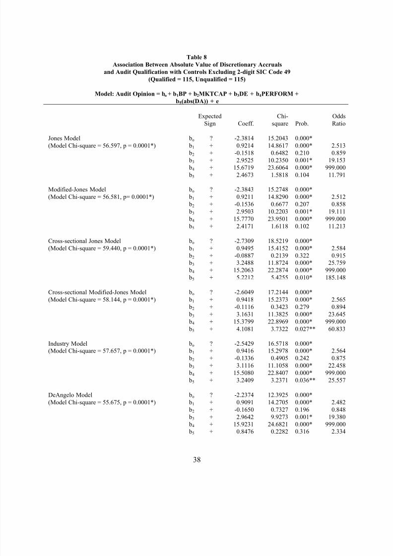
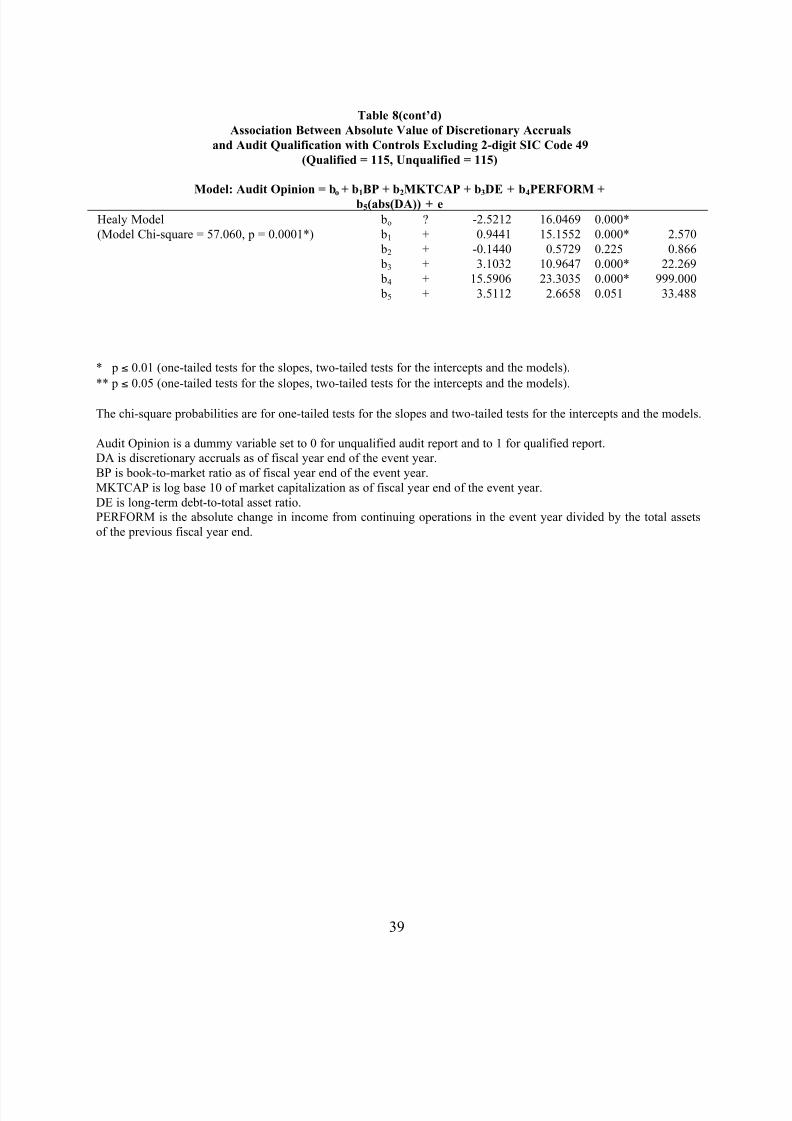
Recall that about 30 percent of our sample firms are in the Electric, Gas, and Sanitary

Service industry (SIC 49). To evaluate whether this subset of firms alone causes our results, we

replicate the tests in Table 7 after removing all firms in this industry. The results displayed in

Table 8 show that the performance of five of the models evaluated remains unchanged.

Specifically, the two cross-sectional models continues to perform well and their time-series

counterparts as well as the DeAngelo Model continue to perform poorly. However, the

performances of the Industry Model and the Healy Model are improved in that the relation

between discretionary accruals and audit qualifications becomes significant for the former and

marginally significant for the latter.

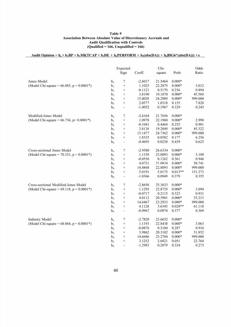
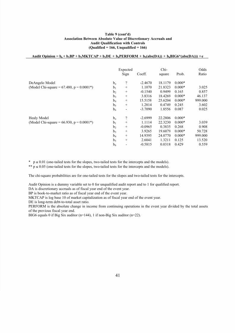
4.3 Big Six Auditors vs. Non-Big Six Auditors

Finally, we assess specifications that consider differential audit quality between Big Six

auditors and non-Big Six auditors. As discussed above, this analysis follows because Big Six

auditors are identified in the literature as higher quality auditors (see, e.g., Palmrose 1988, p. 63)

due to their technological capability in detecting earnings management, and once detected, a

higher probability of reporting it. We thus replicate the logit analysis after adding a dummy

variable on the discretionary accruals variable. This dummy variable is set to zero for Big Six

10The insignificant results for the firm-size variable should be interpreted with caution. This follows

because our test and control samples were matched on firm size. Thus, the insignificant results may follow because

the sample variation with respect to firm size was insufficient to allow the regression to pick up its effect.



24

auditors (144 firms) and to one for non-Big Six auditors (22 firms). Thus, if Big Six auditors are

of higher quality, the coefficient on the additional variable should be negative. Table 9 reports

the results for this sensitivity analysis. The results are consistent with the results for the full

sample reported in Table 7. Specifically, the cross-sectional versions of the Jones Model and the

Modified Jones Models generate significant estimates on the discretionary-accruals variable,

while the other five models continue to perform poorly. The estimates on the additional variable

that captures differential audit quality are, as predicted, negative for all models, but statistically

insignificant. This statistical insignificance may represent low power due to the small number of

firms (22) with a non-Big Six auditor. Overall, these findings reinforce our findings for the full

sample.

5. Conclusion

Prior evaluations of the ability of alternative discretionary-accruals models to separate

earnings to discretionary accruals and nondiscretionary earnings yielded conflicting results.

Dechow, Sloan, and Sweeney (1995) concluded that all models appear well specified, generate

tests of low power for earnings management, and the Modified Jones Model generates the fewest

type II errors. Still, all models reject the null hypothesis of no earnings management at rates

exceeding the specified test-levels when applied to samples of firms with extreme financial

performance. Guay, Kothari, and Watts (1996) attempted to improve on the methodology for

evaluating discretionary-accruals models of this prior research. They first made predictions on

the basis of explicit assumptions regarding the relation between stock returns, and discretionary

accruals and nondiscretionary earnings, and then investigated whether the alternative accrual-

based models produce discretionary accruals and nondiscretionary earnings that conform to their



25

predictions. Unlike Dechow, Sloan, and Sweeney (1995), their findings cast doubts on the

ability of the models to separate accruals into discretionary and nondiscretionary components.

Thus, whether these discretionary-accruals models are able to separate accruals into discretionary

and nondiscretionary components and thereby detect earnings management is still an open

empirical question.

The primary objective of this study is to evaluate the ability of two cross-sectional

models, the Cross-Sectional Jones Model and the Cross-Sectional Modified Jones Model, to

detect earnings management vis-à-vis their time-series counterparts. The motivation follows

because the two cross-sectional models have not been evaluated by prior research, and because,

ex ante, it is unclear which type of model dominates, as each type relies on a different set of

assumptions and it is an empirical question which set is more descriptively valid.

The evaluation involves examining the association between discretionary accruals and

audit qualifications. An association between large discretionary accruals generated by a model

and an audit qualification provides evidence on the ability of the model to detect earnings

management.

Results from univariate chi square tests and logit tests that do not fully control for

potential research confounds show that all models, except the DeAngelo Model, are successful in

discriminating between firms that manage earnings and firms that do not. Once potential

research confounds are controlled, however, only the two cross-sectional models are able to

consistently detect earnings management.

The contribution of this study is twofold. First, we show that the Cross-Sectional Jones

Model and the Cross-Sectional Modified Jones Model, not evaluated by prior research, perform

better than their time-series counterparts in detecting earnings management. This result is



26

important for future earnings management research particularly because using a cross-sectional

model rather than its time-series counterpart should result in a larger sample size that is less

subject to a survivorship bias. It will also allow examining samples of firms with short history.

Second, we demonstrate that correlated omitted variables represent a serious problem for accrual

management studies, and identify three such variables (i.e., book-to-market ratios, financial

leverage, and earnings performance).



27

References

CHANEY, P. K., D. C. JETER, AND C. M. LEWIS. 1995. “The Use of Accruals in Earnings

Management; A Permanent Earnings Hypothesis.” Working paper, VanderbiltUniversity.

CHOI, S. K., AND D.C. JETER. 1992. “The Effect of Qualified Audit Opinion on Earnings

Response Coefficients.” Journal of Accounting and Economics 14, 229-247.

COLLINS, D. W., AND P. Hribar. 1999. “Errors in Estimating Accruals: Implications for

Empirical Research.” Working Paper, University of Iowa.

DEANGELO, L. 1981. “Auditor Size and Auditor Quality.” Journal of Accounting and Economics 1, 113-127.

__________. 1986. “Accounting Numbers as Market Valuation Substitutes: A Study of Management Buyouts of Public Shareholders.” The Accounting Review 61, 400-420.

DECHOW, P.M., R.G. SLOAN, AND A.P. SWEENEY. 1995. “Detecting EarningsManagement.” The Accounting Review 70, 193-225.

DEFOND, M. L., AND J. JIAMBALVO. 1994. “Debt Covenant Violation and Manipulation of

Accruals.” Journal of Accounting and Economics 17, 145-176.

DOPUCH, N., R. HOLTHAUSEN, AND R. LEFTWICH. 1986. “Abnormal Stock ReturnsAssociated with Media Disclosures of ‘Subject to’ Qualified Audit Opinions.” Journal of

Accounting and Economics 8, 93-118.

GUAY, W. R., S. P. KOTHARI, AND R. L. WATTS. 1996. “A Market-Based Evaluation of Discretionary Accrual Models.” Journal of Accounting Research 34 (Supplement), 83-

105.

HANSEN, G. A. 1996. “Do Discretionary Accrual Proxies Measure Earnings Management?”Working paper, University of Rochester.

HEALY, P. M. 1985. “The Effect of Bonus Schemes on Accounting Decisions.” Journal of

Accounting and Economics 7, 85-107.

________. 1996. “Discussion of A Market-Based Evaluation of Discretionary Accrual Models.” Journal of Accounting Research 34, 107-114.

HIRST, D. E. 1994. “Auditor Sensitivity to Earnings Management.” Contemporary Accounting

Research 11, 405-422.





29

Table 1

Summary of the Sample Selection Criteria

Completed firm years 80-97

Less firm years with unqualified or unavailable audit reports

Firm years with qualified audit reports

Less firm years with second or more qualifications during our sample period

Distinct firms with an audit qualification

Less firms with insufficient data for discretionary-accruals calculation

Firms with an audit qualification and data for discretionary-accruals calculation

Less firms with missing control variable data1

Firms with an audit qualification and complete data

Less firms not meeting requirements for matched pair 2

Big Six auditor

non-Big Six auditor

112,384

110,051

2,333

1,464

869

668

201

27

174

8

______

166

144

22

1Firms with a missing or negative book value, missing market value, debt-to-total assets ratio, or earnings are

deleted.

2 An unqualified matched pair control sample was selected based on year, industry, auditor type, and total assets.



30

Table 2

Industry Distribution of Qualified Firm Years by

Two-Digit Standard Industrial Classification Codes

2-Digit

SIC Industry Name

Number

of Observations

13 Oil and Gas Extraction 616 Heavy Constr-Not Bldg Constr 4

17 Construction-Special Trade 1

20 Food and Kindred Products 2

22 Textile Mill Products 2

23 Apparel and Other Finished Pds 2

25 Furniture and Fixtures 2

26 Paper and Allied Products 2

27 Printing, Publishing and Allied 1

28 Chemicals and Allied Products 5

29 Pete Refining and Related Inds 2

30 Rubber and Misc Plastics Prods 2

32 Stone, Clay, Glass, Concrete Pd 133 Primary Metal Industries 9

34 Fabr Metal, Ex Machy, Trans Eq 7

35 Indl, Comml Machy, Computer Eq 13

36 Electr, Oth Elec Eq, Ex Cmp 12

37 Transportation Equipment 5

38 Meas Instr, Photo Gds, Watches 6

42 Motor Freight Trans, Warehous 1

45 Transportation By Air 3

48 Communications 2

49 Electric, Gas, Sanitary Serv 51

50 Durable Goods-Wholesale 3

51 Nondurable Goods-Wholesale 153 General Merchandise Stores 1

54 Food Stores 2

56 Apparel and Accessory Stores 1

58 Eating and Drinking Places 3

62 Security and Commodity Brokers 1

63 Insurance Carriers 1

65 Real Estate 3

70 Hotels, Other Lodging Places 2

73 Business Services 6

78 Motion Pictures 1

---------

Total 166





Table 3 (cont’d)

Descriptive Statistics

*Wilcoxon test (two-tailed). Numbers in parenthesis represent the number of firm-years winsorized and the minimum and maximum before winsorization.

All figures are as of fiscal year end of the event year unless otherwise stated.Total Assets is total liabilities and stockholder’s equity (Compustat data # 6); Current Assets is total current assets (Compustat data # 4); Market Value of Equity is the product of common

outstanding (Compustat data # 25) and the stock price (Compustat data # 199); Book-to-Market Ratio is total common equity (Compustat data # 60) divided by Market Value of Equity; LoDebt / Total Assets is total long term debt (Compustat data # 9) divided by Total Assets; PERFORM is the absolute change in income from continuing operations in the event year (Compu

# 18) divided by Total Assets of previous fiscal year end; Accounts Receivable Turnover Ratio t−

1 is Net Sales divided by the Average Accounts Receivable in year t−

1; Inventory Turnovt−1 is Cost of Goods Sold divided by the Average Inventory in year t−1.



33

Table 4

Comparison of Alternative Expectation Models for Accruals

Model TAt/At-1= α1 (1/At-1) + α2 (∆REVt/At-1) + α3 (PPEt/At-1) + εt

(N = 166)

Model PredictedSign Mean Std Dev Median Minimum Maximum % positive

Number of observations

per regression

TS – Jones 8 0 8 8 8 ---

CS – Jones 109.37 67.80 140 7 232 ---

Estimate of α 1

TS – Jones 14.52 102.07 0.34 -439.95 926.81 55.4

(0.02) (0.16)

CS – Jones 0.02 0.65 0 -3.05 4.52 53.6

(0.96) (0.04)

Estimate of α 2

TS – Jones + 0.10 0.31 0.07 -1.38 1.42 69.9

(0.69) (0.71)

CS – Jones + 0.11 0.11 0.09 -0.17 0.44 84.9

(3.87) (2.98)

Estimate of α 3

TS – Jones - -0.01 0.33 -0.04 -1.87 1.61 29.5

(-0.76) (-0.72)

CS – Jones - -0.05 0.06 -0.04 -0.27 0.21 7.2

(-4.86) (-3.75)

The sample consists of our distinct qualified opinion firms. TS denotes the time-series Jones model originally

proposed by Jones (1991). The time series model is estimated from the past time-series for each firm. CS denotes

the cross-sectional Jones model as proposed by DeFond and Jiambalvo (1994). The cross-sectional Jones model is

similar in form to the time-series Jones model, except it is estimated separately for each combination of calendar

year and 2-digit SIC code. Figures in parentheses denote means/medians of individual regression t-statistics.

TAt is total accruals in year t (the event year).

∆REVt is revenues in year t less revenues in year t-1

PPEt is gross property, plant and equipment at the end of year t

At-1 is total assets at the end of year t-1

εt is the residual



34

Table 5

Association Between Absolute Value of Discretionary Accruals

and Audit Qualifications: Chi-square Test

(Qualified=166, Unqualified=166)

Modified-Jones

X2=7.700

p=0.052

Cross-sectional Jones

X2=17.747

p=0.001

Cross-sectionalModified-Jones

X2=15.557

p=0.002

Industry

X2=9.953

p=0.021

DeAngelo

X2=2.146

p=0.355ualified Unqualified Qualified Unqualified Qualified Unqualified Qualified Unqualified Qualified Unqualified Qualifi

34 33 33 31 35 32 34 29 37 29 37

33 33 34 35 32 30 37 36 31 34 33

28 37 29 36 30 42 24 40 26 36 30

29 39 28 44 23 40 27 37 30 36 31

42 24 42 20 46 22 44 24 42 31 35

166 166 166 166 166 166 166 166 166 166 166

Note: All p-values are one-tailed.



35

Table 6

Association Between Absolute Value of Discretionary Accruals and Audit Qualification

Audit Opinion = bo + b1(abs(DA))+ e

(Qualified = 166, Unqualified = 166)

Expected

Sign Coeff.

Chi-

square Prob.

Odds

Ratio

Jones Model

(Model Chi-square = 4.779, p = 0.0288**)

bo

b1

?

+

-0.2125

3.1506

2.0929

4.6578

0.148

0.015** 23.349

Modified-Jones Model

(Model Chi-square = 4.364, p= 0.0367**)

bo

b1

?

+

-0.2035

2.9510

1.9171

4.2630

0.166

0.020** 19.124

Cross-sectional Jones Model

(Model Chi-square = 9.862, p = 0.0017*)

bo

b1

?

+

-0.3011

4.9327

4.2365

9.2865

0.040**

0.001* 138.752

Cross-sectional Modified-Jones Model


bo

b1

?

+

-0.2621

4.1626

3.2576

7.3559

0.071

0.003* 64.238

Industry Model


bo

b1

?

+

-0.2528

3.4286

2.9311

6.3815

0.087

0.006* 30.834

DeAngelo Model

(Model Chi-square = 1.685, p = 0.1943)

bo

b1

?

+

-0.1211

1.5781

0.7057

1.6696

0.401

0.098 4.846

Healy Model


bo

b1

?

+

-0.2155

3.3573

2.1528

4.7908

0.142

0.014** 28.710

* p ≤ 0.01 (one-tailed tests for the slopes, two-tailed tests for the intercepts and the models).** p ≤ 0.05 (one-tailed tests for the slopes, two-tailed tests for the intercepts and the models).

The chi-square probabilities are for one-tailed tests for the slopes and two-tailed tests for the intercepts.

Audit Opinion is a dummy variable set to 0 for unqualified audit report and to 1 for qualified report.

DA is discretionary accruals.



36

Table 7


and Audit Qualification with Controls


Model: Audit Opinion = bo + b1BP + b2MKTCAP + b3DE + b4PERFORM +

b5(abs(DA)) + e

Expected

Sign Coeff.

Chi-

square Prob.

Odds

Ratio

Jones Model


bo

b1

b2

b3

b4

b5

?

+

+

+

+

+

-2.6179

1.0957

-0.1001

3.8086

15.1437

1.7311

21.9205

22.2425

0.4248

19.2100

24.9181

0.8429

0.000*

0.000*

0.257

0.000*

0.000*

0.179

2.991

0.905

45.087

999.000

5.647


(Model Chi-square = 66.693, p= 0.0001*)

bo

b1

b2

b3

b4

b5

?

++

+

+

+

-2.6231

1.0960-0.0998

3.8110

15.2053

1.7163

22.0092

22.21680.4236

19.2196

25.2553

0.8818

0.000*

0.000*0.258

0.000*

0.000*

0.174

2.9920.905

45.194

999.000

5.564



bo

b1

b2

b3

b4

b5

?

+

+

+

+

+

-2.9669

1.1309

-0.0472

4.0571

14.5769

4.7469

26.8481

22.9547

0.0941

21.0606

23.1894

5.3450

0.000*

0.000*

0.380

0.000*

0.000*

0.010*

3.098

0.954

57.805

999.000

115.230

Cross-sectional Modified-Jones Model(Model Chi-square = 68.935, p = 0.0001*)

bo

b1

b2

b3

b4

b5

?+

+

+

+

+

-2.87271.1258

-0.0634

3.9933

14.7413

3.8348

25.516422.8229

0.1708

20.5708

23.7102

3.8210

0.000*0.000*

0.340

0.000*

0.000*

0.025**

3.083

0.939

54.232

999.000

46.285

Industry Model


bo

b1

b2

b3

b4

b5

?

+

+

+

+

+

-2.7948

1.1159

-0.0772

3.9710

14.7885

2.7961

23.9818

22.8025

0.2517

20.2829

23.7637

2.5227

0.000*

0.000*

0.308

0.000*

0.000*

0.056

3.052

0.926

53.035

999.000

16.380

DeAngelo Model


bo

b1

b2

b3

b4

b5

?

+

+

+

+

+

-2.4789

1.0830

-0.1246

3.7663

15.4954

0.4264

18.5814

21.6083

0.6399

18.2131

25.9926

0.0594

0.000*

0.000*

0.212

0.000*

0.000*

0.404

2.954

0.883

43.219

999.000

1.532



37

Table 7 (cont’d)


and Audit Qualification with Controls


Model: Audit Opinion = bo

+ b1BP + b

2MKTCAP + b

3DE + b

4PERFORM +

b5(abs(DA)) + e

Expected

Sign Coeff.

Chi-

square Prob.

Odds

Ratio

Healy Model


bo

b1

b2

b3

b4

b5

?

+

+

+

+

+

-2.7033

1.1091

-0.0921

3.9165

14.9952

2.4399

22.3840

22.3444

0.3584

19.6378

24.4672

1.3901

0.000*

0.000*

0.275

0.000*

0.000*

0.119

3.032

0.912

50.227

999.000

11.472

* p ≤ 0.01 (one-tailed tests for the slopes, two-tailed tests for the intercepts and the models).

** p ≤ 0.05 (one-tailed tests for the slopes, two-tailed tests for the intercepts and the models).

The chi-square probabilities are for one-tailed tests for the slopes and two-tailed tests for the intercepts and the models.


DA is discretionary accruals as of fiscal year end of the event year.

BP is book-to-market ratio as of fiscal year end of the event year.

MKTCAP is log base 10 of market capitalization as of fiscal year end of the event year.

DE is long-term debt-to-total asset ratio.PERFORM is the absolute change in income from continuing operations in the event year divided by the total assets

of the previous fiscal year end.



38

Table 8


and Audit Qualification with Controls Excluding 2-digit SIC Code 49



+ b1BP + b

2MKTCAP + b

3DE + b

4PERFORM +

b5(abs(DA)) + e

Expected

Sign Coeff.

Chi-

square Prob.

Odds

Ratio

Jones Model


bo

b1

b2

b3

b4

b5

?

+

+

+

+

+

-2.3814

0.9214

-0.1518

2.9525

15.6719

2.4673

15.2043

14.8617

0.6482

10.2350

23.6064

1.5818

0.000*

0.000*

0.210

0.001*

0.000*

0.104

2.513

0.859

19.153

999.000

11.791


(Model Chi-square = 56.581, p= 0.0001*)

bo

b1

b2

b3

b4

b5

?

++

+

+

+

-2.3843

0.9211-0.1536

2.9503

15.7770

2.4171

15.2748

14.82900.6677

10.2203

23.9501

1.6118

0.000*

0.000*0.207

0.001*

0.000*

0.102

2.5120.858

19.111

999.000

11.213



bo

b1

b2

b3

b4

b5

?

+

+

+

+

+

-2.7309

0.9495

-0.0887

3.2488

15.2063

5.2212

18.5219

15.4152

0.2139

11.8724

22.2874

5.4255

0.000*

0.000*

0.322

0.000*

0.000*

0.010*

2.584

0.915

25.759

999.000

185.148

Cross-sectional Modified-Jones Model(Model Chi-square = 58.144, p = 0.0001*)

bo

b1

b2

b3

b4

b5

?+

+

+

+

+

-2.60490.9418

-0.1116

3.1631

15.3799

4.1081

17.214415.2373

0.3423

11.3825

22.8969

3.7322

0.000*0.000*

0.279

0.000*

0.000*

0.027**

2.565

0.894

23.645

999.000

60.833

Industry Model


bo

b1

b2

b3

b4

b5

?

+

+

+

+

+

-2.5429

0.9416

-0.1336

3.1116

15.5080

3.2409

16.5718

15.2978

0.4905

11.1058

22.8407

3.2371

0.000*

0.000*

0.242

0.000*

0.000*

0.036**

2.564

0.875

22.458

999.000

25.557

DeAngelo Model


bo

b1

b2

b3

b4

b5

?

+

+

+

+

+

-2.2374

0.9091

-0.1650

2.9642

15.9231

0.8476

12.3925

14.2705

0.7327

9.9273

24.6821

0.2282

0.000*

0.000*

0.196

0.001*

0.000*

0.316

2.482

0.848

19.380

999.000

2.334



39

Table 8(cont’d)


and Audit Qualification with Controls Excluding 2-digit SIC Code 49



+ b1BP + b

2MKTCAP + b

3DE + b

4PERFORM +

b5(abs(DA)) + e

Healy Model


bo

b1

b2

b3

b4

b5

?

+

+

+

+

+

-2.5212

0.9441

-0.1440

3.1032

15.5906

3.5112

16.0469

15.1552

0.5729

10.9647

23.3035

2.6658

0.000*

0.000*

0.225

0.000*

0.000*

0.051

2.570

0.866

22.269

999.000

33.488



The chi-square probabilities are for one-tailed tests for the slopes and two-tailed tests for the intercepts and the models.





DE is long-term debt-to-total asset ratio.

PERFORM is the absolute change in income from continuing operations in the event year divided by the total assets






Table 9 (cont'd)

Association Between Absolute Value of Discretionary Accruals and

Audit Qualification with Controls


Audit Opinion = bo

+ b1BP + b

2MKTCAP + b

3DE + b

4PERFORM + b

5(abs(DA)) + b

6BIG6*(abs(DA))) +

e

Expected

Sign Coeff.

Chi-

square Prob.

Odds

Ratio

DeAngelo Model


bo

b1

b2

b3

b4

b5

b6

?

+

+

+

+

+

-

-2.4670

1.1070

-0.1540

3.8316

15.5158

1.2814

-3.7090

18.1179

21.8323

0.9499

18.4269

25.6204

0.4749

1.8556

0.000*

0.000*

0.165

0.000*

0.000*

0.245

0.087

3.025

0.857

46.137

999.000

3.602

0.025

Healy Model(Model Chi-square = 66.930, p = 0.0001*)

bo

b1

b2

b3

b4

b5

b6

?+

+

+

+

+

-

-2.69991.1114

-0.0965

3.9265

14.9395

2.6041

-0.5815

22.280622.3230

0.3835

19.6079

24.0770

1.3211

0.0318

0.000*0.000*

0.268

0.000*

0.000*

0.125

0.429

3.039

0.908

50.728

999.000

13.520

0.559



The chi-square probabilities are for one-tailed tests for the slopes and two-tailed tests for the intercepts.





DE is long-term debt-to-total asset ratio.

PERFORM is the absolute change in income from continuing operations in the event year divided by the total assets


BIG6 equals 0 if Big Six auditor (n=144), 1 if non-Big Six auditor (n=22).

Documents

Discretionary-Accruals Models and Audit Qualifications