Embed Size (px)
Citation preview

Contents lists available at ScienceDirect
Journal of Accounting and Economics
Journal of Accounting and Economics 56 (2013) 190–211
0165-41http://d
☆ WeworkshUniversUnivers
n CorrE-m1 Th
variablechangevalue an
journal homepage: www.elsevier.com/locate/jae
Estimation sample selection for discretionaryaccruals models$
Frank Ecker, Jennifer Francis n, Per Olsson, Katherine SchipperFuqua School of Business, Duke University, Durham, NC 27708, United States
a r t i c l e i n f o
Article history:Received 23 March 2012Received in revised form13 July 2013Accepted 25 July 2013Available online 6 August 2013
Keywords:Discretionary accrualsEarnings managementPeer firmsDiscretionary accruals models
JEL Classification:M41M42C12C13C18
01/$ - see front matter & 2013 Elsevier B.V. Ax.doi.org/10.1016/j.jacceco.2013.07.001
appreciate helpful comments from Ross Waop participants at the 2011 Global Issues iity, ESADE Business School, ESSEC, Hong Kongity of Michigan, University of Washington anesponding author. Tel.: +1 919 660 7817; faail address: [email protected] (J. Francis).e accruals models require each observations. For example, the basic Jones model requirein sales revenues, while the Larcker and Richd market value of equity and cash from ope
a b s t r a c t
We examine how the criteria for choosing estimation samples affect the ability to detectdiscretionary accruals, using several variants of the Jones (1991) model. Researchers commonlyestimate accruals models in cross-section, and define the estimation sample as all firms in thesame industry. We examine whether firm size performs at least as well as industry member-ship as the criterion for selecting estimation samples. For U.S. data, we find estimation samplesbased on similarity in lagged assets perform at least as well as estimation samples basedon industry membership at detecting discretionary accruals, both in simulations with seededaccruals between 2% and 100% of total assets and in tests examining restatement data andAAER data. For non-U.S. data, we find industry-based estimation samples result in significantsample attrition and estimation samples based on lagged assets perform at least as well asestimation samples based on industry membership, both in simulations and in tests examiningGerman restatement data, with substantially less sample attrition.
& 2013 Elsevier B.V. All rights reserved.
1. Introduction
Using several variants and extensions of the Jones (1991) model of discretionary accruals, we examine how the selection ofestimation samples affects the power of these models to detect discretionary accruals. Our research aims to provide a practicalsolution to the problem of substantial sample attritionwhen discretionary accruals models are estimated in time series (eliminatingfirms lacking the requisite number of time-series observations) and in industry cross-sections (eliminating firms whose industrieslack the requisite number of members).
The problem we address is significant in the U.S. and acute in non-U.S. markets. The average number of firms per industry inthe U.S. during 1988–2009 with the necessary data to estimate an accruals observation1 is 80.5 (SIC2), 21.7 (SIC3) and 13.6 (SIC4).For the 99 non-U.S. countries with data on Compustat Global over the same time period the corresponding mean values are 3.5
ll rights reserved.
tts (the Editor), Anwer Ahmed (the referee), and from Mary Barth, Dirk Black and Justin Hopkins andn Accounting Conference at the University of North Carolina, Copenhagen Business School, DukePolytechnic University, Stockholm School of Economics, University of Arizona, University of Lancaster,d Yale University. Early drafts were titled "Peer firm selection for discretionary accruals models".x: +1 919 660 7971.
to have current and one-year lagged financial data to construct the dependent and independents data on lagged total assets, current total accruals, current net property, plant and equipment, and theardson (2004) extension of the Jones model requires, additionally, current and lagged receivables, bookrations.
F. Ecker et al. / Journal of Accounting and Economics 56 (2013) 190–211 191
(SIC2), 1.8 (SIC3) and 1.6 (SIC4). Imposing typical requirements—10 observations besides the event firm2 are available for anindustry to be included—leads to substantial sample attrition and the complete elimination of many countries from studies ofdiscretionary accruals. For U.S. data, the use of industry-based estimation samples eliminates 1–22% of the otherwise-availablesample, depending on how industry is defined. For the 69 non-U.S. countries with at least one year with 11 firm-yearobservations overall, the sample loss is between 32% and 93% on average, depending on how industry is defined and theweighting of countries; requiring sufficient data to form industry-based estimation samples for a given country causes between29 and 40 countries (out of 69) to be eliminated entirely from a study that estimates discretionary accruals using estimationsamples defined by industry membership.3
We propose and test a solution to this problem, specifically, basing estimation samples on similarity in size, not industrymembership. We consider size because, as we explain in more detail later, it is an intuitively grounded alternative (toindustry membership) indicator of similarity; that is, a group of larger firms is more alike than is a mixed group of largerand smaller firms. Our solution and related tests derive from two simultaneously-considered objectives: reducing sampleattrition from data requirements and retaining at least the detection power obtainable from using industry membership asthe estimation sample selection criterion. The objective of reducing sample attrition from data requirements suggests thecriterion for choosing estimation samples should be both widely available and numerical, so large samples can be ranked onthe criterion. Size-based estimation samples impose no sample loss incremental to the loss imposed by the accruals modelsthemselves, because size-based peers4 can be defined as firms closest in size to the target firm. Since firms can always beranked on size, there will always be a set of firms in the neighborhood of the target firm. Whether those firms are closeenough for purposes of detecting discretionary accruals is the empirical question we explore.5 Evidence that firm sizeperforms at least as well as industry membership as the criterion for selecting an estimation sample for a discretionaryaccruals model means researchers can substantially expand sample sizes without loss of detection power.
To meet the second (detection power) objective the criterion should also result in estimation samples with reasonablysimilar properties. Our use of firm size as measured by lagged total assets as an estimation sample criterion is based onprevious research showing firms of similar size are also similar with regard to factors associated with accruals, such as growth,complexity and monitoring. Relative to smaller firms, larger firms are likely to be older (so more stable, with lower growthrates), to have more segments (so more complex) and to be more closely monitored (larger analyst following, more regulatoryoversight, greater likelihood of Big-4 auditor, more institutional ownership). More specifically, in a study addressing the use ofindustry membership combined with size to identify peer firms for use in relative performance evaluation, Albuquerque(2009) provides extensive discussion and empirical evidence supporting the view that size subsumes several characteristicsaffecting accruals, including diversification, operating leverage, and growth options. In addition, Kothari et al. (2005) documenta correlation between size and discretionary accruals estimated using an industry-cross-sectional accruals model.
In analyses of the detection-power-related objective, we consider how and why previous research uses industry-basedestimation samples. Our reading of the literature on detecting discretionary accruals suggests researchers have implicitly orexplicitly maintained a three-part presumption: (1) estimation samples for detecting discretionary (managed) accrualsshould be homogeneous with respect to the normal (unmanaged) accruals generating process because (2) similarity in thenormal accruals process is believed to be associated with the power to detect abnormal accruals, and (3) firms in the sameindustry have congruent normal accruals generating processes.6
Our research mainly aims to shed light on the first two components of this three-part presumption.7 With regard tothe first component, our results suggest both size-based samples and industry-based samples exhibit reasonable, andreasonably similar, evidence of accruals homogeneity. For example, the explanatory power of the Jones model with interceptfor industry-based estimation samples is about 51–52% while the explanatory power of this model for the lagged assets-based estimation samples is about 44%. We conclude that if sample attrition is not a concern, industry-based samplesproduce higher explanatory power in the estimation of normal accruals; if sample attrition is a concern, the researcherwould trade off a reduction in explanatory power with a loss in sample size. However, inconsistent with the secondcomponent of the three-part presumption, we find lagged assets-based estimation samples produce higher detection ratesof abnormal (or discretionary) accruals, as compared to industry-based estimation samples. That is, our evidence supportsthe first presumption and refutes the second presumption: while industry-based estimation samples have the highest
2 The event firm is the firm whose discretionary accruals are the subject of the researcher's analysis.3 The researcher could pool data across countries, within industry, to increase the number of firms in each industry. This pooling has the potential to
introduce noise that lowers the power of the test. If the researcher aims to examine jurisdictional influences on discretionary accruals, pooling observationsacross jurisdictions is either not feasible or will bias the results against detecting such influences.
4 Consistent with the notion that estimation samples for both normal accruals estimation and abnormal or discretionary accruals detection shouldhave a reasonable degree of homogeneity with respect to the accruals generating process, we sometimes refer to estimation samples as “peer firms.” Forexample, estimation samples based on industry membership are “industry peers” or “industry-based peers” and estimation samples based on size are “sizepeers” or “size-based peers.”
5 Our tests also address the fact that the larger population of U.S. traded firms relative to any non-U.S. market implies size-based neighbors in the U.S.will (likely) be more similar to the target firm than are neighbors in non-U.S. markets.
6 Researchers have questioned the empirical validity of the assumption that firms in the same industry (same SIC code) have congruent normalaccruals (e.g., Bernard and Skinner, 1996; Brickley and Zimmerman, 2010). Dopuch et al. (2012) find little support for the assumption that firms in the sameindustry have a homogeneous accruals-generating process; they do not propose an alternative to industry for defining an estimation sample.
7 We provide supplementary analyses in Section 6.6 on the third component.
F. Ecker et al. / Journal of Accounting and Economics 56 (2013) 190–211192
explanatory power for normal accruals, these same models are not the best at detecting abnormal accruals (rather, size-based samples generally dominate here).
We compare the power to detect discretionary accruals using industry-based estimation samples with the detectionpower of size-based samples using both simulations and archival tests. Our tests modify the approach used by Dechow et al.(1995) to examine the power of several accruals models to detect earnings management. Their aim was to compare accrualsmodels, whereas we compare the effects of estimation sample selection for a given set of models. Dechow et al. estimatedaccruals models using time-series data,8 while our focus is on cross-sectional estimation using industry-based versus size-based criteria for estimation sample selection. We use Dechow et al.'s framework to guide our analysis and to assist thereader in interpreting our results.
Our first simulations use all firms, both U.S. and Canadian, with available data on Compustat North America over 1951–2009;we refer to these firms as the U.S. data or the U.S. sample. These simulation tests reveal that estimation samples based on laggedassets are at least as powerful as industry peers at detecting induced discretionary accruals, and they are often more powerful.Our first archival tests consider the power of size-based and industry-based peer groups to detect discretionary accruals for twosamples of restatement firms and firms named in an SEC Accounting and Auditing Enforcement Release (AAER firms).9 Thesefirms are known to have discretionary accruals, because a restatement or AAER is after-the-fact evidence of purposefulor inadvertent deviation from a normal (GAAP-based) accruals-generating process, but the amounts may be unknown tothe researcher. These tests show that models estimated using lagged-asset-based estimation samples have higher rates ofdiscretionary accruals detection than do estimations using industry-based estimation samples. Our second simulation tests focuson non-U.S. data, specifically, Compustat Global data for 1988–2009. We find size-based peers perform as well as, or better than,industry-based peers at detecting induced discretionary accruals and impose far less sample attrition. Our second archival tests,using German restatement data, support the conclusions based on our analyses of U.S. restatement/AAER data: using industry-based estimation samples results in significant sample loss, and size-based estimation samples yield better detection results thando industry-based estimation samples.
These results are robust to a battery of sensitivity tests and additional analyses, including variations in the numbers of firmsincluded in industry-based and size-based estimation samples. We also provide evidence that the performance of estimationsamples based on lagged assets is not induced by the inclusion of lagged assets in the accruals models we analyze.
Viewed as a whole, our results indicate size-based estimation samples perform at least as well as industry-basedestimation samples in terms of detecting discretionary accruals in both U.S. data and non-U.S. data. The use of size-basedestimation samples for U.S. data avoids sample losses (up to 22% in some cases) arising from using industry-basedestimation samples. Our results have even greater practical value for estimating discretionary accruals models using non-U.S. data, where basing estimation samples on industry membership results in sample attrition as high as 90%. Entirecountries excluded from industry-based estimations can be included in size-based estimations, with no loss of power todetect discretionary accruals.
The remainder of the paper is organized as follows. Section 2 provides descriptive evidence on our sample. Section 3reports the results of a simulation analysis investigating the power of size-based and industry-based peer groups to detectinduced discretionary accruals using U.S. data. Section 4 analyzes the ability of estimations using industry-based peers andsize-based peers to detect discretionary accruals of restatement firms and AAER firms. Section 5 reports results of analysesof non-U.S. data, including both simulation tests and tests for detection of discretionary accruals in German restatementfirms. Section 6 reports additional tests and section 7 concludes.
2. Sample and descriptive data
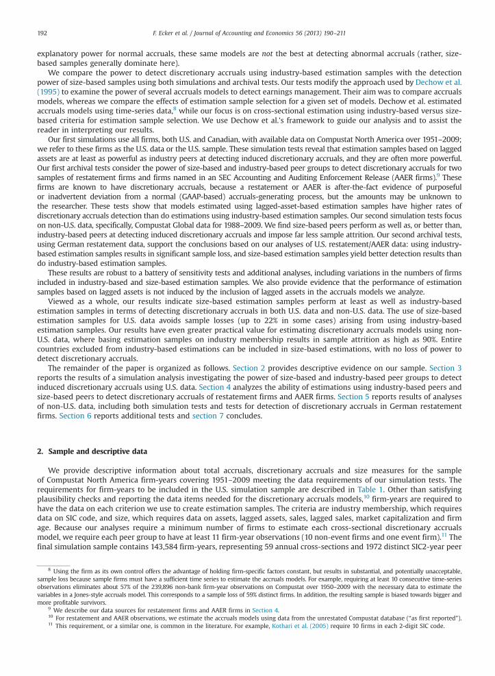
We provide descriptive information about total accruals, discretionary accruals and size measures for the sampleof Compustat North America firm-years covering 1951–2009 meeting the data requirements of our simulation tests. Therequirements for firm-years to be included in the U.S. simulation sample are described in Table 1. Other than satisfyingplausibility checks and reporting the data items needed for the discretionary accruals models,10 firm-years are required tohave the data on each criterion we use to create estimation samples. The criteria are industry membership, which requiresdata on SIC code, and size, which requires data on assets, lagged assets, sales, lagged sales, market capitalization and firmage. Because our analyses require a minimum number of firms to estimate each cross-sectional discretionary accrualsmodel, we require each peer group to have at least 11 firm-year observations (10 non-event firms and one event firm).11 Thefinal simulation sample contains 143,584 firm-years, representing 59 annual cross-sections and 1972 distinct SIC2-year peer
8 Using the firm as its own control offers the advantage of holding firm-specific factors constant, but results in substantial, and potentially unacceptable,sample loss because sample firms must have a sufficient time series to estimate the accruals models. For example, requiring at least 10 consecutive time-seriesobservations eliminates about 57% of the 239,896 non-bank firm-year observations on Compustat over 1950–2009 with the necessary data to estimate thevariables in a Jones-style accruals model. This corresponds to a sample loss of 59% distinct firms. In addition, the resulting sample is biased towards bigger andmore profitable survivors.
9 We describe our data sources for restatement firms and AAER firms in Section 4.10 For restatement and AAER observations, we estimate the accruals models using data from the unrestated Compustat database (“as first reported”).11 This requirement, or a similar one, is common in the literature. For example, Kothari et al. (2005) require 10 firms in each 2-digit SIC code.
Table 1Selection of data observations for simulation using U.S. data 1950–2009.
Selection criteria # Firm-years
Unique firm-years on Compustat North America 408,245Observations for firms with more than 1 year of data 407,726With lagged total assets, total assets, sales4¼1, ROA4¼�1 299,414With data for total accruals calculation 247,841Non-bank firm-years 239,896With data for identifying ALL peer groups 203,842With at least 11 firm-year observations per SIC4 143,584
Firms per peergroup-year
Peer group # Firm-years # Peergroup-years Mean Min Median Max
Entire cross-section 143,584 59 2434 15 2442 5683SIC2 143,584 1972 73 11 37 958SIC3 143,584 4349 33 11 18 824SIC4 143,584 5486 26 11 17 436
This table reports the sample restrictions imposed by requirements to have the necessary data to calculate an accruals observation, to identify peer groups,and to estimate the accruals models. The most restrictive criterion requires 10 non-event firms in the same SIC4 code. The bottom rows of the table reportthe sizes of the industry peer groups, e.g., out of the 143,584 firm-year observations meeting our requirements, there are 1972 distinct SIC2-year peergroups.
Table 2Descriptive statistics for U.S. samples.
# Obs. Mean Std. dev. P5 P25 Median P75 P95
Total accruals 143,584 �0.0310 0.3312 �0.2215 �0.0897 �0.0391 0.0126 0.1863Total accruals (GAO restatements) 1337 �0.0702 0.1895 �0.2491 �0.1070 �0.0572 �0.0139 0.0925Total accruals (AA restatements) 5032 �0.0455 0.3451 �0.2331 �0.1004 �0.0487 �0.0008 0.1593Total accruals (AAER) 372 0.0174 0.8024 �0.2966 �0.0722 �0.0034 0.1225 0.5586
Abs. total accruals 143,584 0.1059 0.3154 0.0063 0.0309 0.0642 0.1188 0.3000Abs. total accruals (GAO restatements) 1337 0.1051 0.1726 0.0060 0.0334 0.0705 0.1221 0.2745Abs. total accruals (AA restatements) 5032 0.1151 0.3285 0.0068 0.0325 0.0682 0.1208 0.3100Abs. total accruals (AAER) 372 0.2310 0.7686 0.0065 0.0368 0.0879 0.2072 0.7717
Total assets 143,584 1662 8672 5.28 26.83 104.77 531.32 6419.31Lagged total assets 143,584 1528 8091 4.42 22.68 90.45 466.25 5870.00Sales 143,584 1364 7698 4.05 25.27 103.60 499.23 5214.00Lagged sales 143,584 1264 7269 3.05 21.54 90.51 447.74 4824.60Market cap. 143,584 1647 11,050 2.87 18.80 88.03 482.85 5406.10Firm age (in years) 143,584 15.54 14.39 2.00 6.00 11.00 21.00 46.00ROA 143,584 �0.01 0.20 �0.39 �0.02 0.04 0.07 0.15
This table presents descriptive information about accruals (signed and absolute) for firm-years in the U.S. simulation sample, the U.S. GAO and AuditAnalytics (AA) restatement samples and the U.S. AAER sample. Total accruals are as defined in the text. Total assets and sales are from Compustat. Firm ageis defined as the maximum difference, in years, between the date of the fiscal year end and the founding year as available on Jay Ritter's website (http://bear.warrington.ufl.edu/ritter/ipodata.htm), or the first year with data on Compustat, or the first year with data on CRSP. ROA is net income beforeextraordinary items scaled by total assets.
F. Ecker et al. / Journal of Accounting and Economics 56 (2013) 190–211 193
groups (4349 distinct SIC3-year peer groups and 5486 distinct SIC4-year peer groups). On average, the industry-year peergroups contain 73 firms (SIC2), 33 firms (SIC3) and 26 firms (SIC4).
Table 2 reports descriptive statistics on total accruals (signed and absolute) for the U.S. simulation sample, for tworestatement samples and for one AAER sample. The first restatement sample contains 1337 U.S. General Accounting Office(GAO) restatement firm-years; the second restatement sample contains 5032 Audit Analytics (AA) restatement firm-years;the AAER sample contains 372 firm-years. For the simulation sample, we provide data on the size-based criteria foridentifying peer firms: assets, lagged asset, sales, lagged sales, market capitalization, and firm age. These data show mean(median) total accruals for the simulation sample are �3.1% (�3.9%) of total assets, with a standard deviation of 33.12%. Incontrast, mean (median) accruals for the GAO restatement sample, the AA restatement sample and the AAER sample are�7.0% (�5.7%), �4.6% (�4.9%) and 1.7% (�0.34%), respectively. Standard deviations of accruals for these three samples are18.95% (GAO restatements), 34.51% (AA restatements), and 80.24% (AAERs).
F. Ecker et al. / Journal of Accounting and Economics 56 (2013) 190–211194
3. Simulations with seeded discretionary accruals
This section describes our simulation analyses of how choosing estimation samples based on size versus industrymembership affects the ability to detect seeded discretionary accruals. We first describe the models for discretionaryaccruals and the estimation samples we consider. Section 3.2 outlines the setup of our simulations, Section 3.3 describes ourdesign choices and Section 3.4 presents the simulation results. Section 3.5 presents results of analyses shedding light on thereasons for those results.
3.1. Discretionary accruals estimation and estimation samples
In our main tests, we conduct tests on three cross-sectional discretionary accruals models used in the literature.12 Themodels are based on the following three equations:
Total accrualsi;tTotal Assetsi;t�1
¼ α11
Total Assetsi;t�1þ α2
ΔSalesi;tTotal Assetsi;t�1
þ α3Net PPEi;t
Total Assetsi;t�1þ DAJones
i;t ð1Þ
Total accrualsi;tTotal Assetsi;t�1
¼ α0 þ α11
Total Assetsi;t�1þ α2
ΔSalesi;tTotal Assetsi;t�1
þ α3Net PPEi;t
Total Assetsi;t�1þ DAJonesðinterceptÞ
i;t ð2Þ
Total accrualsi;tTotal Assetsi;t�1
¼ α0 þ α11
Total Assetsi;t�1þ α2
ΔSalesi;t�ΔARi;t
Total Assetsi;t�1þ α3
Net PPEi;tTotal Assetsi;t�1
þ DAMod: Jonesi;t ð3Þ
where Total accrualsj,t¼firm j's total accruals in year t, measured as the change in current assets (adjusted for the change incash) minus the change in current liabilities (adjusted for current liabilities used for financing) minus depreciation expense;Total Assetsj,t�1¼firm j's total assets in year t�1; ΔSalesj,t¼firm j's change in sales between year t�1 and year t; Net PPEj,t¼firm j's net property, plant and equipment in year t; ΔARj,t¼firm j's change in accounts receivable between year t�1 andyear t; ROAj,t¼firm j's return on assets in year t.
Eqs. (1) and (2) are the Jones (1991) model without and with an intercept, introduced and recommended by Kothari et al.(2005). Eq. (3) is a modified Jones model which includes an intercept and an adjustment for the change in accountsreceivable. The residuals from estimating Eqs. in the cross section provide three types of discretionary accruals.
Our benchmark estimation sample is a peer group formed by a random selection of firms from the entire sample crosssection.13 We define industry-based estimation samples (industry peers) based on 2-digit, 3-digit and 4-digit SIC codes,because our reading of the literature suggests these are the most commonly-used approaches to determining estimationsamples for discretionary accruals models.14 We define size-based estimation samples (size peers) based on total assets, laggedtotal assets, sales, lagged sales, market capitalization and firm age.15 Varying the cross section (“peer group”) over which thediscretionary accruals models are estimated yields a peer-group-dependent measure and distribution of discretionary accruals.
3.2. Simulation design, seeding and estimation sample evaluation via rejection rates
Using the firm-years from the sample described in Table 1, we perform 100 iterations, each of which has four steps:
1.
Rich
pow
We randomly select 500 firm-years and define them as event-firm-years. The event-firm-years remain constantthroughout the iteration.
2.
For each event-firm-year, we select initial peer firms from which estimation samples will be chosen:a. Sample cross section.b. Industry-based peer groups (SIC2 industry, SIC3 industry, SIC4 industry) chosen by matching by year and industry,regardless of the number of firm-years in the industry.c. Size-based peer groups (total assets, lagged total assets, sales, lagged sales, market capitalization, firm age) chosen by
matching the year and the 25 adjacent (to the event firm) lower-ranked firms and the 25 adjacent (to the event firm)higher-ranked firms; these are the event firm's “closest neighbors.”
12 Ward13 W14 R15 Wer
Step 2 yields varying numbers of observations in the sets of initial peer firms; they vary for the four industry-based peergroups and are fixed at 50 for the six size-based peer groups.
3.
To equalize the number of observations in each peer group, we randomly select 10 firms from the initial peer groupsidentified in Step 2. This step is intended to equalize the power of tests, which is affected by sample size. We use ae discuss results based on other models, including variants of performance-adjusted accruals based on Kothari et al. (2005) and Larcker andson's (2004) extension of the Jones model, in Section 6.3.e do not consider double-sorted peer groups (firms from the same industry and same size decile), because our goal is to relax sample restrictions.esults of sensitivity tests related to industry definitions are discussed in Section 6.e also examined ROA-based peer groups. Results (not tabulated) indicate ROA-based estimation samples have discretionary accruals detection
that is marginally better than reported for the entire cross section.
sele
F. Ecker et al. / Journal of Accounting and Economics 56 (2013) 190–211 195
constant number of peer firms (10), both to estimate the discretionary accruals regression and for the significance test onthe difference in discretionary accruals between event and non-event observations.
4.
We repeat Steps 2 and 3 for each of the 500 event-firm-years.Our simulation tests are based on 100 iterations, yielding 50,000 event-firm-years, each matched with 10 peer-firm-years from each of the 10 peer group definitions. While this design does not impose restrictions on how often a firm-yearcan be selected, either as an event observation or a non-event observation, the two-layer sampling minimizes the likelihoodan entire subsample would be replicated.
For each event-firm-year, we seed discretionary accruals into the data. First, we calculate the event-firm-year's ratio oftotal accruals to lagged total assets (the dependent variable in the accruals model regressions). We add between 2% and 20%of lagged total assets, in two percentage point increments, to yield 10 “positively managed” accruals figures for each event-firm-year. As a reference, Dechow et al. (1995) seed discretionary accruals in 10 percentage point increments, from 0% to100%. While we also calculate results for 20–100% seed levels16 we focus on smaller amounts of induced discretionaryaccruals in the tables (20% or less), because we believe they are more descriptive of observed levels of discretionary accruals.In particular, Table 2 shows the 5th and 95th percentiles of scaled signed accruals for the U.S. simulation sample are about�22% and +19%, respectively; the unsigned percentiles are 0.6% (5th percentile) and 30% (95th percentile). The 0% seed casereflects 0% discretionary accruals as proxied by the raw Compustat data.
Our main simulations investigate the ability to detect an amount (between 2% and 20%) of seeded discretionary accrualsat the subsample level. For each peer firm definition, we obtain 50,000 subsamples, each one containing one event-firmmatched with 10 peer firms, and each one containing the 10 levels of seeded accruals. These seeded amounts represent thediscretionary accruals that are the object of the discretionary accruals detection tests. Our tests compare the estimateddiscretionary accruals of the event-firm-years with the average of the estimated discretionary accruals of the 10 non-event-firm-years, using the following regression, separately for each seed level:
Discretionary accrualsi;t ½εi;t �½0%;2%;4%;:::;20%� ¼ α½0%;2%;4%;:::;20%�0 þ α½0%;2%;4%;:::;20%�
1 Event Dummyi;t þ ηi;t ð4Þ
where EventDummy¼1 for the single event-firm observation in each subsample. We assess detection power by counting thenumber of positive α1 coefficients significant at the 10% level.17 The detection rate is the fraction, out of 50,000, of significantcoefficients.
3.3. Explanation of simulation choices
In this section, we describe the reasoning for four design choices used in the simulation. First, we believe the two-layerselection of peer firms, as described in Section 3.2, captures a typical setting faced by a researcher whose objective is toidentify discretionary accruals. For example, there are typically a limited number of “event” firm-years, each of which ishypothesized to contain discretionary accruals of some (perhaps unspecified) amount and sign. In all likelihood, the sampleand data restrictions in a typical discretionary accruals study are more constraining than suggested by the comprehensivedataset from which we initially select peer firms in Step 2. We use the Step-3 selection to capture the effects of theconstrained sample size of a typical discretionary accruals study. The second selection layer ensures a constant number ofpeer firms and ensures our results are not driven by using the closest size-based neighbors in the estimation sample.18
Second, in selecting neighbors for the size-based peer groups, we form relative peer groups (i.e., peers are defined as theevent firm's closest-in-size neighbors) not absolute peer groups (i.e., peers are determined using an absolute size cutoff).For example, an absolute size peer group would contain firms from the same asset decile or market capitalization decile asthe event firm, where the cutoff values for those deciles are determined using the entire cross-section of firms; the event-firm is then matched to firms from its same decile. We believe the absolute peer group approach has at least twodisadvantages compared to the relative peer group approach. First, the absolute approach does not ensure symmetry in theselection of peer firms; for example, non-event firms from the same decile will be systematically smaller (larger) when theevent firm is a large (small) firm in that decile. Second, the absolute peer group approach requires the full cross-section offirms to determine the initial partitions (e.g., asset deciles or market capitalization deciles). Forming initial deciles/partitionsusing a subsample of 500 firms yields different results than does forming deciles/partitions using a subsample of 5000 firms,particularly if the 500 firm subsample is not distributed uniformly across the deciles of the 5000-firm subsample, but, say,biased towards bigger and more profitable firms.
A third design choice concerns the interaction between seeded discretionary accruals and the models of discretionaryaccruals. We seed discretionary accruals by adding between 2 and 20 percentage points to the event-firm's ratio of totalaccruals to lagged assets. We do not adjust other variables such as sales or total assets. Our seeding, therefore, is most
16 These results are not tabulated; inferences based on these results are similar to those reported in the paper.17 We find similar results (not tabulated) using 5% and 1% significance levels.18 As a sensitivity test, we select the 10 closest-in-size peers. Results (not tabulated) show this lagged asset peer group performs better than the one wect based on the random sampling in Step 3.
F. Ecker et al. / Journal of Accounting and Economics 56 (2013) 190–211196
similar to Dechow et al.'s (1995) “expense manipulation” view of discretionary accruals (although our approach is cross-sectional and theirs is time-series).19
Modeling other financial statement effects requires additional assumptions, as summarized and applied by Dechow et al.(1995). A specific form of earnings management affects specific income statement and/or balance sheet accounts that mightor might not be included as independent variables in the normal accruals model, and a guiding principle of such models isthat the independent variables should not be affected by earnings management. Put another way, the ability to detect agiven type of earnings management will be affected by the choice of the normal accruals model itself, because certain typesof earnings management might affect the variables in one model, but not those in another model. In an extreme case inwhich both accruals (the dependent variable) and an independent variable change by equal amounts, earnings managementwould remain undetected. We acknowledge that the choice of a specific accruals model is important for the detection of agiven type of earnings management. Because we do not compare accruals models (the focus of Dechow et al., 1995), wefocus on the simplest (from a modeling perspective) view of discretionary accruals which does not adjust the values of theindependent variables in the accruals models. The independent variables of all models can thus be assumed to be unaffectedby (our seeded) earnings management, and hence we do not induce varying detection power across models.
A fourth design choice concerns the level of the analysis. As previously described, we analyze detection rates at thesubsample level (50,000 subsamples each consisting of 1 event firm and 10 non-event firms) rather than at the moreaggregated sample level (100 samples each consisting of 500 event firms and 5000 non-event firms). We select thesubsample level for two reasons. First, as a practical matter, the discretionary accruals estimation must be performed at thesubsample level, so the finer data are readily available. Second, it is hard to observe differences at the sample level becausefirm-specific idiosyncrasies are averaged out, implying that even at small seeded discretionary accruals levels detectionrates will approach 100% quickly for all models. Stated differently, we believe performing our analysis at the sample level(where the number of event firms and non-event firms is large) would mislead readers about the generalizability ofour findings to the smaller samples typically used in discretionary accruals research. By analyzing subsamples, we believewe more closely approximate the issues faced in discretionary accruals research.
3.4. Results of simulations
Table 3 reports for each discretionary accruals model (panels of table) and peer group definition (columns of table) thefraction of times, as a percentage of the 50,000 subsamples, the α1 coefficient from Eq. (4) is significantly positive at the 10%level for increasing levels of seeded discretionary accruals (the seed levels are the rows of each panel). We refer to therejection rate, at the 10% level, as the discretionary accruals detection rate. Results for the 0% seed level correspond tothe benchmark case of no seeded discretionary accruals and can be used to gauge the validity of the approach. Specifically,if there are no discretionary accruals and if the data are truly random, 5% of cases should exhibit significant positivediscretionary accruals at the 10% level (5% of cases will show significant negative discretionary accruals). A 95% confidenceinterval around this theoretical rejection rate ranges from 0.7% to 9.3% for samples of 100 observations. Table 3 shows thedetection rates for the 0% seed level are close to 5% for all peer definitions and models, although there is some evidence the0% detection rates are higher for the lagged asset-based estimation sample.20 These rejection rates are well within the limitsof the 95% confidence interval and are not statistically different from 5% or each other.
Turning to the non-zero seed levels, our interest is in which peer group (column) yields the highest detection rates acrossaccruals models. These results show that for all seed levels, the peer group formed using the cross-section performs theworst; this result is expected since this peer group does not attempt to match non-event firms with event-firms on anydimension except the event year. Peer groups based on firm age, sales and market capitalization also perform poorly acrossall seed levels. At seed levels less than 10%, the industry-based peers and lagged asset-based peers have the highestdetection rates, and these rates are similar. At seed levels between 10% and 20%, the detection rate of the lagged asset-basedpeers begins to exceed the others.
We create two measures of the aggregate performance of each peer group across the 10 seed levels for each model. Ourfirst measure of the performance of a given peer group/model/seed level combination is the detection rate achieved by aspecified peer group, for each model and seed level, divided by the maximum detection rate achieved by any peer group forthat seed level/model combination. We average this peer group/model/seed level performance measure across the seedlevels for each model and peer group, to yield an “effectiveness score” for each peer group/model combination. The closerthe effectiveness score to 100% (the value if the peer group had the highest detection rate for every seed level), the better at
19 Dechow et al. also model earnings management as “revenue manipulation” and “margin manipulation.” In the revenue manipulation scenario, theyadd the seeded discretionary accruals to total accruals, sales and accounts receivable. For the models given by Eqs. (1) and (2), the change in sales wouldincrease; however, the modified model (Eq. (3)) is not affected because the increase in sales is offset by the same increase in accounts receivable. In themargin manipulation scenario, they introduce a magnifier, defined as the net profit margin, to translate a specified change in total accruals to a (bigger)change in sales and accounts receivable. Again, this affects the models which contain the change in sales, but does not affect the modified models becausethe bigger change in sales is offset by the same bigger change in accounts receivable.
20 Sensitivity tests reported in Section 6 show these slightly elevated rejection rates are largely driven by our choice of 10 peer firms. The rejectionrates in the 0% seed case do not propagate into higher detection rates for positive seed levels. We find that increasing the number of size-based peer firms(which can be done without sample loss) leads to lower benchmark rejection rates, but not necessarily to lower detection rates for the positive seed levels.
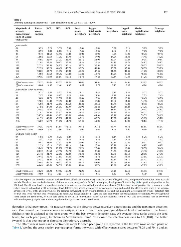
Table 3Detecting earnings management I – Base simulation using U.S. data, 1951–2009.
Magnitude ofaccrualsmanagement(in % of laggedtotal assets)
Entirecrosssection
SIC2 SIC3 SIC4 Totalassetsneighbors
Laggedtotal assetsneighbors
Salesneighbors
Laggedsalesneighbors
Marketcapitalizationneighbors
Firm ageneighbors
Jones model0% 5.2% 5.2% 5.3% 5.3% 5.0% 5.8% 5.2% 5.1% 5.2% 5.2%2% 6.9% 7.8% 8.1% 8.1% 7.4% 8.3% 7.1% 7.1% 7.2% 7.2%4% 9.3% 11.6% 12.5% 12.4% 11.0% 11.9% 9.9% 10.2% 10.2% 10.4%6% 12.6% 16.5% 17.7% 17.7% 15.7% 17.0% 14.0% 14.3% 14.4% 14.2%8% 16.9% 22.0% 23.2% 23.5% 21.1% 22.9% 19.0% 19.2% 19.3% 19.1%10% 21.9% 27.8% 29.1% 29.3% 27.3% 29.3% 24.4% 24.7% 24.8% 24.1%12% 27.3% 33.5% 34.8% 35.1% 33.7% 35.5% 29.9% 30.3% 30.7% 29.6%14% 32.9% 39.2% 40.4% 40.7% 39.7% 41.6% 35.6% 35.9% 36.3% 35.2%16% 38.6% 44.7% 45.7% 45.9% 45.2% 47.3% 41.0% 41.3% 41.7% 40.7%18% 43.9% 49.6% 50.7% 50.8% 50.2% 52.7% 45.9% 46.3% 46.6% 45.8%20% 49.1% 54.0% 55.1% 55.1% 54.7% 57.4% 50.8% 50.8% 51.2% 50.5%
Effectiveness score 78.3% 94.0% 98.0% 98.3% 92.6% 98.9% 84.1% 84.9% 85.6% 84.3%Effectiveness rank 10.00 4.50 2.40 1.90 4.50 1.70 8.30 7.30 6.20 8.20
Jones model (with intercept)0% 5.2% 5.2% 5.3% 5.3% 5.1% 5.8% 5.2% 5.2% 5.2% 5.2%2% 7.1% 7.8% 8.1% 8.2% 7.4% 8.5% 7.3% 7.3% 7.2% 7.4%4% 9.6% 11.7% 12.5% 12.5% 11.0% 12.3% 10.3% 10.5% 10.4% 10.7%6% 12.8% 16.4% 17.4% 17.4% 15.8% 17.0% 14.1% 14.4% 14.3% 14.4%8% 16.9% 21.7% 22.6% 22.6% 21.2% 22.5% 18.7% 19.2% 18.9% 18.7%10% 21.5% 27.3% 28.0% 28.3% 26.9% 28.4% 23.8% 24.2% 24.2% 23.6%12% 26.4% 32.5% 33.2% 33.7% 32.7% 34.0% 28.8% 29.3% 29.4% 28.6%14% 31.4% 37.5% 38.3% 38.8% 38.2% 39.8% 33.9% 34.2% 34.5% 33.7%16% 36.7% 42.4% 43.1% 43.6% 43.4% 44.9% 38.8% 39.0% 39.3% 38.6%18% 41.5% 46.8% 47.6% 47.9% 48.1% 49.7% 43.2% 43.5% 43.8% 43.1%20% 46.0% 50.7% 51.6% 51.7% 52.4% 53.9% 47.5% 47.9% 48.1% 47.4%
Effectiveness score 79.1% 94.3% 97.5% 98.1% 93.7% 99.5% 84.7% 85.7% 85.6% 85.0%Effectiveness rank 10.00 4.50 2.90 2.00 4.00 1.60 8.10 6.90 6.90 8.10
Modified Jones model0% 5.5% 5.3% 5.3% 5.4% 5.1% 6.1% 5.2% 5.3% 5.2% 5.3%2% 7.1% 7.8% 8.1% 8.3% 7.5% 8.5% 7.2% 7.3% 7.2% 7.4%4% 9.4% 11.6% 12.3% 12.4% 11.0% 12.2% 10.2% 10.4% 10.3% 10.4%6% 12.5% 16.1% 17.1% 17.1% 15.6% 16.8% 13.8% 14.1% 14.1% 14.1%8% 16.4% 21.2% 22.2% 22.3% 21.2% 22.0% 18.3% 18.8% 18.5% 18.4%10% 20.7% 26.5% 27.5% 27.7% 26.8% 27.8% 23.2% 23.6% 23.5% 23.0%12% 25.4% 31.7% 32.6% 32.8% 32.3% 33.3% 28.1% 28.5% 28.6% 27.7%14% 30.4% 36.7% 37.5% 37.8% 37.9% 38.7% 33.0% 33.3% 33.6% 32.7%16% 35.3% 41.4% 42.1% 42.5% 43.1% 43.9% 37.6% 38.1% 38.4% 37.3%18% 39.9% 45.7% 46.6% 46.7% 47.7% 48.6% 42.0% 42.5% 42.9% 41.7%20% 44.4% 49.6% 50.5% 50.6% 51.8% 52.7% 46.2% 46.5% 47.2% 45.8%
Effectiveness score 78.2% 94.2% 97.5% 98.2% 94.8% 99.6% 84.3% 85.5% 85.6% 84.4%Effectiveness rank 10.00 4.60 3.10 2.10 3.60 1.60 8.30 6.90 6.70 8.10
This table reports the detection rates for each seed level of induced discretionary accruals (2–20% of lagged assets) and peer definitions, for three accrualsmodels. The detection rate is the fraction of times, as a percentage of the 50,000 subsamples, the slope coefficient in Eq. (4) is significantly positive at the10% level. The 0% seed level is a specification check, insofar as a well-specified model should show a 5% detection rate of positive discretionary accruals(when none is induced) at a 10% significance level. Effectiveness scores are reported for each peer group and model; the effectiveness score is the average,across seed levels, of the absolute value of the distance between the peer group's detection rate and the maximum (across all peer groups) detection ratefor that seed level. For each seed level (row) and model, we assign a rank of 1 (10) to the peer group with the best (worst) detection rate. We average theseranks across the seed levels, for each peer group, to obtain an “effectiveness rank”. An effectiveness score of 100% and effectiveness rank of 1.0 wouldindicate the peer group is best at detecting discretionary accruals across seed levels.
F. Ecker et al. / Journal of Accounting and Economics 56 (2013) 190–211 197
detection is that peer group. This measure captures the distance between a given detection rate and the maximum detectionrate. Our second performance measure assigns a rank to each peer group/model/seed level combination; the lowest(highest) rank is assigned to the peer group with the best (worst) detection rate. We average these ranks across the seedlevels, for each peer group, to obtain an “effectiveness rank”. The closer the effectiveness rank to 1.0 (10.0), the better(worse) is that peer group at detecting discretionary accruals.
The effectiveness scores and effectiveness ranks for each peer group are reported in the last two rows of each panel ofTable 3. We find the cross-section peer group performs the worst, with effectiveness scores between 78.2% and 79.1% and an
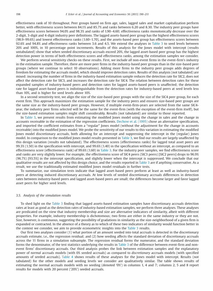
F. Ecker et al. / Journal of Accounting and Economics 56 (2013) 190–211198
effectiveness rank of 10 throughout. Peer groups based on firm age, sales, lagged sales and market capitalization performbetter, with effectiveness scores between 84.1% and 85.7% and ranks between 6.20 and 8.30. The industry peer groups haveeffectiveness scores between 94.0% and 98.3% and ranks of 1.90–4.60; effectiveness ranks monotonically decrease over the2-digit, 3-digit and 4-digit industry peer definitions. The lagged assets-based peer group has the highest effectiveness scores(98.9–99.6%) and lowest effectiveness ranks (1.60–1.70), and the assets-based peer group has effectiveness scores between92.6% and 94.8% and effectiveness ranks between 3.6 and 4.5. We extend the analyses in Table 3 to seed levels between20% and 100%, in 10 percentage point increments. Results of this analysis for the Jones model with intercept (resultsuntabulated) show that when seeded discretionary accruals exceed 20%, the lagged asset-based peer group has the highestdetection power in terms of both effectiveness scores and effectiveness ranks, among the estimation samples we consider.
We perform several sensitivity checks on these results. First, we include all non-event firms in the event-firm's industryin the estimation sample. Therefore, there are more peer firms in the industry-based peer groups than in the size-based peergroups (where we continue to select 10 observations). Adding more firms to the industry peer groups adds degrees offreedom for estimating the accruals model, which should improve detection rates. Results of this analysis (not tabulated) aremixed: increasing the number of firms in the industry-based estimation sample reduces the detection rate for SIC2, does notaffect the detection rate for SIC3, and increases the detection rate for SIC4. The relation between detection rates for theseexpanded samples of industry-based peers and detection rates for lagged assets-based peers is unaffected; the detectionrate for lagged asset-based peers is indistinguishable from the detection rates for industry-based peers at seed levels lessthan 10%, and is higher for seed levels above 10%.
In a second sensitivity test, we align the size of the size-based peer groups with the size of the SIC4 peer group, for eachevent firm. This approach maximizes the estimation sample for the industry peers and ensures size-based peer groups arethe same size as the industry-based peer groups. However, if multiple event-firm-years are selected from the same SIC4-year, the industry peer firms selected will be the same for the event-firm (with the exception of the event-firm itself), butthe size-based estimation samples might shift considerably. Results (not tabulated) are similar to those reported.
In Table 3, we present results from estimating the modified Jones model using the change in sales and the change inaccounts receivable in the estimation of the regression coefficients. Dechow et al. (1995) chose an alternative specification,and imported the coefficient estimates from a “regular” Jones model (without the adjustment for the change in accountsreceivable) into the modified Jones model. We probe the sensitivity of our results to this variation in estimating the modifiedJones model discretionary accruals, both allowing for an intercept and suppressing the intercept in the (regular) Jonesmodel. In comparison to the modified Jones model results presented in Table 3, we find our results are largely unaffected bythis design variation (results not tabulated). The effectiveness scores (effectiveness ranks) for lagged total asset peers are99.3% (1.50) in the specification with intercept, and 99.6% (1.40) in the specification without an intercept, as compared to aneffectiveness score (effectiveness rank) of 99.6% (1.60) in Table 3. For the industry peer samples, we find effectiveness scoreand ranks are very slightly lower. For example, the effectiveness score of SIC4 peers (SIC3 peers) [SIC2 peers] drops to 96.9%(96.7%) [93.5%] in the intercept specification, and slightly lower when the intercept is suppressed. We conclude that ourqualitative results are not affected by this design choice, and the results reported in Table 3 are if anything conservative. As aresult, we use the traditionally estimated modified Jones model residuals in further tests.
To summarize, our simulation tests indicate that lagged asset-based peers perform at least as well as industry-basedpeers at detecting induced discretionary accruals. At low levels of seeded discretionary accruals differences in detectionrates between industry-based peers and lagged asset-based peers are small; the differences become larger and favor laggedasset peers for higher seed levels.
3.5. Analysis of the simulation results
To shed light on the Table 3 finding that lagged assets-based estimation samples have discretionary accruals detectionrates at least as good as the detection rates of industry-based estimation samples, we perform three analyses. These analysesare predicated on the view that industry membership and size are alternative indicators of similarity, albeit with differentproperties. For example, industry membership is dichotomous; two firms are either in the same industry or they are not.Size, however, is continuous, suggesting the possibility of gradations in similarity as the size-neighborhood of a given firm isexpanded or contracted. In the absence of a theory as to which of these two indicators of similarity would function better inthe context we consider, we aim to provide econometric insights into the Table 3 results.
Our first two analyses consider (1) what portion of an amount seeded into total accruals is detected in the discretionaryaccruals estimate, i.e., the regression residual; and (2) how seeding affects the standard deviation of discretionary accrualsacross the 11 firms in a simulation subsample. The regression residual forms the numerator, and the standard deviationforms the denominator, of the test statistics underlying the results in Table 3 of the difference between event-firm and non-event firms' discretionary accruals. Our third analysis probes the link between estimation samples and the explanatorypower of normal accruals models (with 0% seeded accruals) as compared to discretionary accruals models (with specifiedamounts of seeded accruals). Table 4 shows results of these analyses for the Jones model with intercept. Results (nottabulated) for the other models and seeding levels we consider are qualitatively similar. The table shows results ofestimating the normal accruals models with no seeding (denoted ‘0%’) in columns 1, 4 and 7; columns 2, 5 and 8 reportresults for models with 20 percent (‘20%’) seeded accruals.
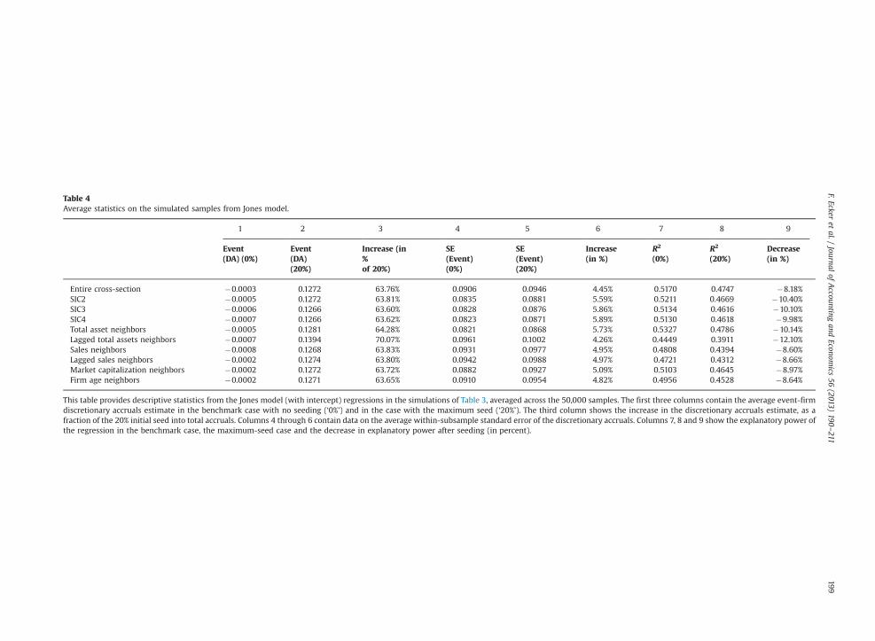
Table 4Average statistics on the simulated samples from Jones model.
1 2 3 4 5 6 7 8 9
Event(DA) (0%)
Event(DA)(20%)
Increase (in%of 20%)
SE(Event)(0%)
SE(Event)(20%)
Increase(in %)
R2
(0%)R2
(20%)Decrease(in %)
Entire cross-section �0.0003 0.1272 63.76% 0.0906 0.0946 4.45% 0.5170 0.4747 �8.18%SIC2 �0.0005 0.1272 63.81% 0.0835 0.0881 5.59% 0.5211 0.4669 �10.40%SIC3 �0.0006 0.1266 63.60% 0.0828 0.0876 5.86% 0.5134 0.4616 �10.10%SIC4 �0.0007 0.1266 63.62% 0.0823 0.0871 5.89% 0.5130 0.4618 �9.98%Total asset neighbors �0.0005 0.1281 64.28% 0.0821 0.0868 5.73% 0.5327 0.4786 �10.14%Lagged total assets neighbors �0.0007 0.1394 70.07% 0.0961 0.1002 4.26% 0.4449 0.3911 �12.10%Sales neighbors �0.0008 0.1268 63.83% 0.0931 0.0977 4.95% 0.4808 0.4394 �8.60%Lagged sales neighbors �0.0002 0.1274 63.80% 0.0942 0.0988 4.97% 0.4721 0.4312 �8.66%Market capitalization neighbors �0.0002 0.1272 63.72% 0.0882 0.0927 5.09% 0.5103 0.4645 �8.97%Firm age neighbors �0.0002 0.1271 63.65% 0.0910 0.0954 4.82% 0.4956 0.4528 �8.64%
This table provides descriptive statistics from the Jones model (with intercept) regressions in the simulations of Table 3, averaged across the 50,000 samples. The first three columns contain the average event-firmdiscretionary accruals estimate in the benchmark case with no seeding (‘0%’) and in the case with the maximum seed (‘20%’). The third column shows the increase in the discretionary accruals estimate, as afraction of the 20% initial seed into total accruals. Columns 4 through 6 contain data on the average within-subsample standard error of the discretionary accruals. Columns 7, 8 and 9 show the explanatory power ofthe regression in the benchmark case, the maximum-seed case and the decrease in explanatory power after seeding (in percent).
F.Eckeret
al./Journal
ofAccounting
andEconom
ics56
(2013)190
–211199
F. Ecker et al. / Journal of Accounting and Economics 56 (2013) 190–211200
The average event firm residual from estimating a normal (no seeded discretionary accruals) model, reported in column 1,shows all estimation samples21 function well in terms of yielding minimal evidence of abnormal accruals; that is,the measure of abnormal accruals is miniscule for all estimation samples, with average residuals ranging from �0.0002 to�0.0008. The largest negative residuals are associated with the SIC4, lagged assets and sales-based estimation samples, suggesting,if anything, there is a bias against detecting seeded positive discretionary accruals for these estimation samples. Column 2 displaysthe residuals resulting from seeding 20% discretionary accruals into the event firm's total accruals. Column 3 shows the portion ofthe seeded amount transferred into the discretionary accruals estimate as a percentage of the 20% seed. To the extent the seededaccrual influences the regression coefficients (i.e., the seeding changes the results of estimating the model of normal accruals), theresiduals will increase by less than 20%; if the regression coefficients are entirely unaffected by the presence of the seeded accrual,the entire seeded amount will translate into the residual. For all but the lagged-asset-based estimation samples, the models detectbetween 63.6% and 64.3% of the seeded accruals; for the lagged-asset-based estimation samples, the residuals increase by 70% ofthe seed. This result suggests that more of the seeded accrual appears in the regression residual for estimation samples based onlagged assets, thus contributing to the detection power of the size-based estimation samples.
We next consider how the seeded accrual affects the standard deviation of discretionary accruals estimates within thesample of 11 firms. Columns 4 and 5 report the average standard deviation of residuals in the no-seed case and the 20%-seedcase, respectively, followed by column 6 containing the percentage increase due to the seeding. These standard deviations,which would be the denominators in tests of differences in the discretionary accruals, will increase in the presence ofseeded abnormal accruals, because the seeding adds an amount to the dependent variable that should not be explained bythe explanatory variables. Results show the increases in standard deviation range from 4.3% (lagged assets) to 5.9% (SIC4),with increases generally smaller for the size-based estimation samples than for the industry-based estimation samples.Combined with the previously discussed finding, this result suggests the detection power of lagged-assets-based estimationsamples derives from both a numerator effect (a larger mapping of the seeded accruals amount into the regression residual,the discretionary accruals estimate) and a denominator effect (a smaller standard deviation of residuals).
The preceding analyses show that differences in discretionary accruals detection rates for different types of estimationsamples are linked to the extent to which the seeding of accruals affects the regression model itself, and therefore the regressionresiduals. To provide more evidence on this point, we focus on the average (over 50,000 samples) explanatory power for thezero-seed benchmark accruals model (column 7) and the 20%-seed accruals model (column 8). Column 9 reports the decrease inexplanatory power when we seed 20% accruals, as an inverse measure of the extent to which the regression is influenced by theseeding. The lagged-assets-based estimation sample shows the largest decrease in explanatory power when abnormal accrualsare seeded, about �12.1% (from column 9) and the lowest cross-sectional explanatory power for normal accruals, about 44.5%(from column 7); explanatory power for the other normal accruals models ranges from about 53.3% (total assets) to 47.2% (laggedsales) and the decline in explanatory power ranges from 10.4% (SIC2) to 8.2% (entire cross section).
We interpret these results as follows. First, viewing size and industry membership as two alternative measures of similarity,we would expect both size-based estimation samples and industry-based estimation samples to have substantial explanatorypower for normal accruals models. We confirm this expectation, and also find industry-based models tend to have higherexplanatory power for normal accruals. Second, seeding discretionary accruals increases only a single dependent variableobservation (the event firm); detection power stems from the extent to which this single-observation increase in thedependent variable appears in the error term as opposed to influencing the regression coefficients. If the regressioncoefficients do not change at all, the entire seeded amount appears in the error term and would therefore be detected asdiscretionary accruals. The larger the decline in explanatory power of a model with seeded accruals, as compared to a model ofnormal accruals with zero seeding, the greater the portion of the seeded amount appearing in the error term (the unexplainedportion of the shifted dependent variable). We find both industry-based and size-based estimation samples exhibit over 8percentage point decreases in explanatory power in the presence of seeded accruals, and the decrease is largest for the lagged-assets-based estimation sample—that is, the seeding shifts the lagged-assets-based regression coefficients least.
Econometrically, therefore, the detection power of estimation samples based on lagged total assets derives from their relativelymore robust, relatively more stable, regression coefficients in the presence of seeded discretionary accruals. Put another way, usingestimation samples based on size results in a greater portion of a seeded amount appearing in the error term, the unstandardizedmeasure of discretionary accruals, as opposed to in a shift in the regression coefficients. Although prior research has, perhapsimplicitly, assumed that explanatory power for normal accruals is tantamount to detection power for abnormal accruals, our resultssuggest a tradeoff between two alternative indicators of similarity. Specifically, if the focus is on the explanatory power of a modelof normal accruals, using industry-based estimation samples increases explanatory power and likely results in smaller sample sizes.However, if the focus is on detection power, as is the case in much earnings management research, using lagged assets-basedestimation samples does not sacrifice detection power and substantially increases sample sizes.
4. Tests on restatement firms and AAER firms
In this section, we examine the performance of industry-based and size-based estimation samples in detecting unusuallevels of absolute discretionary accruals in firm-years with after-the-fact acknowledged abnormal accruals. We analyze
21 Recall the event firms are held constant while non-event peers vary according to estimation sample definition.
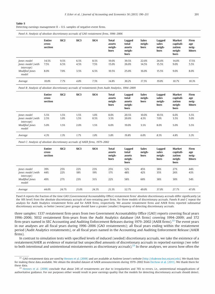
Table 5Detecting earnings management II – U.S. samples of negative-event firms.
Panel A: Analysis of absolute discretionary accruals of GAO restatement firms, 1996–2006
Entirecrosssection
SIC2 SIC3 SIC4 Totalassetsneigh-bors
Laggedtotalassetsneigh-bors
Salesneigh-bors
Laggedsalesneigh-bors
Marketcapitali-zationneigh-bors
Firmageneig-hbors
Jones model 14.5% 9.5% 6.5% 8.5% 19.0% 39.5% 22.0% 26.0% 14.0% 17.5%Jones model (withintercept)
7.5% 6.5% 4.5% 7.5% 15.0% 26.0% 14.5% 15.5% 9.0% 5.5%
Modified Jonesmodel
8.0% 7.0% 3.5% 6.5% 10.5% 25.0% 16.0% 15.5% 9.0% 8.0%
Average 10.0% 7.7% 4.8% 7.5% 14.8% 30.2% 17.5% 19.0% 10.7% 10.3%
Panel B: Analysis of absolute discretionary accruals of restatements from Audit Analytics, 1994–2009
Entirecrosssection
SIC2 SIC3 SIC4 Totalassetsneigh-bors
Laggedtotalassetsneigh-bors
Salesneigh-bors
Laggedsalesneigh-bors
Marketcapitali-zationneigh-bors
Firmageneig-hbors
Jones model 5.5% 1.5% 1.5% 1.0% 8.0% 20.5% 10.0% 10.5% 6.0% 5.5%Jones model (withintercept)
2.5% 1.0% 1.5% 0.5% 3.5% 20.0% 4.5% 7.0% 3.5% 5.0%
Modified Jonesmodel
5.0% 1.5% 2.0% 1.5% 6.0% 19.0% 3.5% 8.0% 5.0% 5.5%
Average 4.3% 1.3% 1.7% 1.0% 5.8% 19.8% 6.0% 8.5% 4.8% 5.3%
Panel C: Analysis of absolute discretionary accruals of AAER firms, 1979–2002
Entirecrosssection
SIC2 SIC3 SIC4 Totalassetsneigh-bors
Laggedtotalassetsneigh-bors
Salesneigh-bors
Laggedsalesneigh-bors
Marketcapitali-zationneigh-bors
Firmageneig-hbors
Jones model 39% 25% 22% 23% 25% 52% 45% 38% 27% 44%Jones model (withintercept)
44% 22% 18% 19% 17% 48% 42% 35% 26% 43%
Modified Jonesmodel
49% 27% 23% 31% 22% 58% 60% 38% 30% 54%
Average 44.0% 24.7% 21.0% 24.3% 21.3% 52.7% 49.0% 37.0% 27.7% 47.0%
Panel A reports the fraction of the time GAO (Governmental Accountability Office) restatement firms’ absolute discretionary accruals differ significantly (atthe 10% level) from the absolute discretionary accruals of non-restating peer firms, for three models of discretionary accruals. Panels B and C repeat theanalysis for Audit Analytics restatement firms and for AAER firms, respectively. We assume restatement firms and AAER firms reported substantialdiscretionary accruals, so better (worse) peer groups should have a greater (smaller) frequency of detecting discretionary accruals.
F. Ecker et al. / Journal of Accounting and Economics 56 (2013) 190–211 201
three samples: 1337 restatement firm-years from two Government Accountability Office (GAO) reports covering fiscal years1996–2006; 5032 restatement firm-years from the Audit Analytics database (AA firms) covering 1994–2009; and 372firm-years named in SEC Accounting and Auditing Enforcement Releases during 1979–2002 (AAER firms).22 The event yearsin our analyses are all fiscal years during 1996–2006 (GAO restatements); all fiscal years ending within the restatementperiod (Audit Analytics restatements), or all fiscal years named in the Accounting and Auditing Enforcement Release (AAERfirms).
In contrast to simulation tests with specified levels of induced (seeded) discretionary accruals, we take the existence of arestatement/AAER as evidence of material but unspecified amounts of discretionary accruals in reported earnings (we referto both intentional and unintentional misstatements as discretionary accruals).23 In these analyses, we assess how often the
22 GAO restatement data are used by Hennes et al. (2008) and are available at Andrew Leone's website (http://sbaleone.bus.miami.edu). We thank himfor making these data available. We obtain the detailed dataset of AAER announcements during 1979–2002 from Dechow et al. (2011). We thank them forthese data.
23 Hennes et al. (2008) conclude that about 24% of restatements are due to irregularities and 76% to errors, i.e., unintentional misapplications ofauthoritative guidance. For our purposes either would result in poor earnings quality that the models for detecting discretionary accruals should detect.
F. Ecker et al. / Journal of Accounting and Economics 56 (2013) 190–211202
restatement/AAER firm's estimated absolute discretionary accruals exceed the estimated absolute discretionary accruals ofits peer firms. Under the view that restatement/AAER firms have, in fact, managed earnings such that their absolutediscretionary accruals are larger than those of their peers, larger detection rates indicate the peer group is better at detectingdiscretionary accruals.
Our analyses of discretionary accruals are performed at the iteration level; we perform 200 iterations. To analyze the GAOrestatement sample, we first select 100 event-firm-years from the population of Compustat firms with restatements; anevent-firm-year is a firm-year with a restatement announcement in the 11 months following the fiscal-year end.24 For eachevent-firm-year, we randomly select 10 non-restating firms from the same year and from each peer group, where the 10peer groups are as previously defined. We estimate the discretionary accruals models for each sample consisting of oneevent-firm and 10 peer firms, generating residuals for each of the 11 firms. We pool the absolute values of these residuals atthe iteration level, generating 100 event-firm absolute residuals and 1000 peer firm absolute residuals per iteration. Wefocus on absolute discretionary accruals to avoid directional predictions of the intentional earnings manipulation or theunintentional error leading to the restatement.
For each iteration, we compare the mean absolute residual for the 100 event-firms with the mean absolute residual ofthe 1000 non-event firms, calculating a t-statistic for the difference. After 200 iterations, we have 200 t-statistics for thedifferences in mean absolute residuals.25 Because we focus on observed restatements/AAERs containing presumed materialdiscretionary accruals, we expect the t-statistics to be significantly positive. The detection rate is the frequency of significantt-statistics, as a percentage of the 200 iterations. Our analyses focus on how the choice of peer groups affects this detectionrate: holding the event firms constant, better (worse) peer groups will have larger (smaller) detection rates. Because ourassumptions that restatement firms have managed or misstated their accruals and the accruals management affects thefiscal year prior to the restatement announcement may not hold for all observations, we do not expect to observe 100%detection rates.
Table 5 reports the detection rates, defined as the fraction of iterations where the t-statistic is significant at the 10% levelor better; rows correspond to the accruals models and columns correspond to the peer groups. In panel A, the results for theGAO restatement sample show the lagged asset-based peer group has the highest average detection rate of 30.2%, rangingbetween 25.0% and 39.5%, depending on the accruals model. The other estimation samples yield average detection ratesbetween 4.8% (SIC3) and 19.0% (lagged sales). In panel B, the results for the Audit Analytics restatement sample supportsimilar inferences; the average detection rate for the lagged asset-based peer group is 19.8% (the range is 19.0–20.5%), whilethe average detection rates for other estimation samples range from 1.0% (SIC4) to 8.5% (lagged sales). Panel C, contains theresults of the AAER analysis. Compared to the samples of restatement firms, overall detection rates increase substantially,consistent with an increased severity of accounting violations of AAER firms as compared to (possibly voluntary)restatements. The average (across accruals models) detection rate for the lagged assets estimation sample is 52.7%, rangingfrom 48% to 58%, and the other estimation samples show average detection rates between 21% (SIC3) to 49% (sales).
These findings from analyses of restatement firms and AAER firms are consistent with our simulation results: both showlagged assets work at least as well as, and sometimes better than, estimation samples based on industry membership indetecting discretionary accruals. We corroborate these findings by repeating our analyses using signed discretionaryaccruals (results not tabulated). In these analyses, we assess the frequency of significant differences in discretionary accrualsat the 10% level, regardless of whether the differences are positive or negative. Overall detection rates across all estimationsamples for both the two restatement samples and the AAER sample tend to increase compared to the tabulated results,although the detection rates for the entire cross-section and lagged asset-based estimation sample decrease slightly.Industry-based estimation sample detection rates average 22.5% across three industry definitions, models and samples ofrestatement/AAER firms, and the lagged-asset-based estimation sample shows the highest average detection rate, 31.8%.
5. Estimation sample selection for analyses of discretionary accruals in non-U.S. data
This section considers the relative power of industry-based estimation samples versus size-based estimation samplesin detecting discretionary accruals in non-U.S. data. Section 5.1 provides evidence on the restrictiveness of industrymembership as the sample selection criterion in non-U.S. markets, characterized by considerably fewer firms than the U.S.markets. Section 5.2 provides simulation-based evidence on the discretionary accruals detection power of industry-basedpeers versus size-based peers using non-U.S. data, and Section 5.3 summarizes key findings and inferences. Section 5.4reports the results of our analysis of German restatement firms.
5.1. Restrictiveness of industry-based estimation samples in non-U.S. data
As discussed in the introduction, using industry-based peers to estimate discretionary accruals models imposes moresubstantial sample attrition for non-U.S. data than for U.S. data. To see this, we impose the same data requirements on
24 Analyses of the Audit Analytics restatement sample and the AAER sample follow the same design; because of differences in population size, weadjust the size of the event sample to 200 (Audit Analytics sample) and 50 (AAER sample). To decrease the probability of duplicating an event sample, weuse 100 iterations of the simulation for the AAER sample (as opposed to 200 for the GAO and Audit Analytics samples).
25 This test is statistically equivalent to the approach used in the simulations tests, a regression on an event-firm dummy variable.
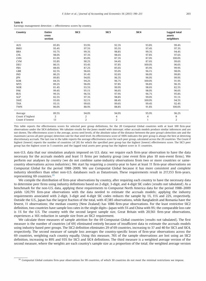
Table 6Earnings management detection — effectiveness scores by country.
Country Entirecrosssection
SIC2 SIC3 SIC4 Lagged totalassetsneighbors
AUS 85.8% 93.9% 92.3% 93.8% 99.4%BMU 95.4% 97.5% 95.5% 97.4% 97.3%BRA 93.7% 99.3% 98.8% 99.3% 94.4%CHL 98.0% 97.3% 98.6% 97.8% 97.6%CHN 81.0% 85.0% 87.3% 87.0% 100.0%CYM 93.8% 90.2% 94.4% 87.6% 99.6%DEU 86.1% 93.4% 97.8% 100.0% 96.6%FRA 88.6% 87.2% 85.6% 85.9% 99.9%GBR 82.5% 96.6% 95.0% 96.1% 98.0%IND 86.2% 91.4% 92.6% 96.0% 99.8%JPN 89.8% 94.8% 96.3% 96.0% 99.9%KOR 84.3% 94.2% 96.7% 100.0% 91.9%MYS 89.2% 96.0% 97.8% 96.8% 96.3%NOR 81.4% 93.5% 99.9% 98.6% 82.5%PAK 99.4% 95.1% 96.6% 98.0% 96.6%RUS 99.3% 96.5% 97.9% 96.7% 95.8%SGP 82.5% 97.3% 98.8% 99.0% 91.1%SWE 93.6% 92.1% 88.4% 100.0% 94.5%THA 93.1% 99.6% 99.6% 99.4% 92.4%TWN 86.0% 88.9% 88.8% 91.8% 100.0%
Average 89.5% 94.0% 94.9% 95.9% 96.2%Count if highest 2 2 4 4 8Count if lowest 13 2 2 1 2
This table reports the effectiveness scores for selected peer group definitions, for the 20 Compustat Global countries with at least 100 firm-yearobservations under the SIC4 definition. We tabulate results for the Jones model with intercept; other accruals models produce similar inferences and arenot shown. The effectiveness score is the average, across seed levels, of the absolute value of the distance between the peer group's detection rate and themaximum (across all peer groups) detection rate for that seed level. An effectiveness score of 100% indicates the peer group is always the best at detectingdiscretionary accruals. The last row in the table reports the average effectiveness score for each peer group, calculated across the 20 countries. The Count ifhighest (lowest) reports the number of countries (of 20) for which the specified peer group has the highest (lowest) effectiveness score. The SIC3 peergroup has the highest score in 5 countries and the lagged total assets peer group has the highest score in 11 countries.
F. Ecker et al. / Journal of Accounting and Economics 56 (2013) 190–211 203
non-U.S. data that our simulation analysis imposed on U.S. data: we require each firm-year observation to have the datanecessary for the accruals models and least 11 firms per industry group (one event firm plus 10 non-event firms). Weperform our analyses by country (we do not combine same-industry observations from two or more countries or same-country observations across industries). We start by requiring a country-year to have at least 11 firm-year observations onCompustat Global for the period 1988–2009. We use Compustat Global because it has more consistent and completeindustry identifiers than other non-U.S. databases such as Datastream. These requirements result in 217,153 firm-years,representing 69 countries.26
We compile the distribution of firm-year observations by country, after requiring each country to have the necessary datato determine peer firms using industry definitions based on 2-digit, 3-digit, and 4-digit SIC codes (results not tabulated). As abenchmark for the non-U.S. data, applying these requirements to Compustat North America data for the period 1988–2009yields 120,791 firm-year observations with the data needed to estimate the accruals models; applying the industryrequirements associated with 2-digit, 3-digit and 4-digit SIC codes reduces the sample by 1%, 11% and 22%, respectively.Outside the U.S., Japan has the largest fraction of the total, with 47,385 observations, while Bangladesh and Romania have thefewest, 11 observations; the median country (New Zealand) has 1086 firm-year observations. For the least restrictive SIC2definition, two countries have sample loss rates in the single digits—Japan with 5% and China with 9%; the comparable loss rateis 1% for the U.S. The country with the second largest sample size, Great Britain with 20,561 firm-year observations,experiences a 16% reduction in sample size from an SIC2 requirement.
We calculate three measures of sample attrition for the 69 Compustat Global countries (results not tabulated). The firstmeasure is the number of countries (of 69) eliminated entirely because of insufficient data to estimate the accruals modelsusing industry-based peer groups. The SIC2 definition eliminates 29 of 69 countries, increasing to 37 and 40 for SIC3 and SIC4,respectively. The second measure of sample loss averages the country-specific losses of firm-year observations across the69 countries, weighting each country equally. Using this measure, 76% of the sample observations are lost using an SIC2definition, increasing to 89% and 93% for SIC3 and SIC4 definitions. The third measure is a weighted average version of thesecond measure, where the weights are each country's sample size as a proportion of the total; the weighted average version
26 Compustat Global contains firm-year observations for 99 countries, of which 30 countries do not meet the minimal restrictions we impose.
F. Ecker et al. / Journal of Accounting and Economics 56 (2013) 190–211204
produces smaller measures of sample loss because it counts the sample loss for Japan (Bangladesh and Romania) more (less) inthe overall measure. Weighted average sample losses are 32% (SIC2), 59% (SIC3) and 70% (SIC4).
The results of this analysis show that requiring the necessary data to estimate accruals models at the industry level imposessignificant sample attrition on non-U.S. data, and even eliminates a substantial number of countries. In contrast, using a size-based estimation sample generates no sample attrition beyond the loss imposed by the accruals model itself. Basing estimationsamples on similarity in lagged assets instead of industry membership, therefore, offers the possibility of much larger samples,including more countries. That said, in a country with relatively few firms, the average size-spread within a size-based peergroup could be large, which could reduce the power of size-based peers to detect discretionary accruals. Therefore, it is anempirical question whether the detection power of size-based peers is as good as the detection power of industry-based peersin countries other than the U.S.
5.2. Detecting induced discretionary accruals in non-U.S. data
We compare industry-based and size-based peer groups in terms of their ability to detect discretionary accruals in non-U.S. data. Our analysis applies the simulation tests reported in Table 3 to each of the 69 countries with available data, andrestricts the simulations to 50 event firms in each of 100 iterations. The most restrictive requirement is that for eachrandomly selected event firm there be 10 non-event firm observations in a 4-digit SIC code for that country. Only 29 of 69non-U.S. countries meet this requirement; of these, nine countries have too few observations (less than 100 firm-years) toperform the bootstrapping required by our simulation. We therefore analyze the “restricted sample” of 20 countries with atleast 100 firm-year observations identifiable under SIC4.
For this “restricted sample,” we analyze the performance of industry-based and size-based peer groups at detectinginduced discretionary accruals. We tabulate results for the Jones model with intercept and for the entire cross-section, threeindustry-based peers, and lagged asset-based peers. Results (not tabulated) for the other models and peer groups yieldsimilar inferences. We analyze all seed levels and report results for the aggregate effectiveness score which averagesdetection rates (measured relative to the best detection rate for that seed level) across all seed levels.27 We also report acount of how many times (of the 20 restricted sample countries) a specified peer group has the highest effectiveness score.The results, reported in Table 6, show the lagged asset-based peer group has the highest average effectiveness score (96.2%)calculated across the 20 countries and a higher effectiveness score for more individual countries than any industry-basedpeer group (for example, the lagged asset peer group has the highest effectiveness score in 8 countries versus 4 countries forboth the SIC3 and SIC4 peer groups).
The tests reported in Table 6 hold the size of each peer group constant at 11 observations (one event firm plus 10 non-event firms). Applying this requirement to industry-based peer groups results in substantial sample loss, especially for SIC4.Given that lagged assets-based peers perform better than industry-based peers for the constant-size peer groups, weinvestigate the performance of lagged asset-based peers when we do not impose the industry requirements. Basingestimation samples on similarity in lagged assets imposes no incremental sample loss, so in theory we can perform thisanalysis for the 69 Compustat Global countries with at least 11 observations in a given year. Because we require each countryto have at least 100 firm-year observations (to perform the bootstrapping required by our simulation), we analyze the 58non-U.S. countries with at least 100 firm-year observations. The detection rates for these 58 countries (not tabulated) showthe lagged asset-based peers detect the seeded discretionary accruals 25.9% of the time at a 10% seed level in the Jonesmodel with intercept. For the 20 countries in both the restricted sample and the 58-country sample, there will bedifferences in detection rates from including additional data when there are no industry restrictions. For these 20 countries,the average detection rate at a 10% seed level in the Jones model with intercept when industry data are required is 24.7%;this detection rate is not reliably different at conventional levels from the 25.9% detection rate for the 58-country sample.Results for other seed levels and other models yield similar inferences.
5.3. Summary of simulation analyses involving non-U.S. data
We draw two inferences from simulation analyses of non-U.S. data. First, estimating discretionary accruals models usingnon-U.S. data and industry-based peers results in significant sample attrition. As a result, researchers may face the problemof low detection power for discretionary accruals and may find the analysis restricted to the few countries with marketslarge enough to support the data requirements (Japan, China, Great Britain). Alternatively, the researcher could aggregatedata across countries, within industry, to increase the number of firm-year observations per industry. This approach treatsall observations for a given industry, across countries, as similar, so it ignores the influence of jurisdiction-specific factors(e.g., accounting standards, legal systems, degree of market development). This approach is problematic if the researcher isinterested in whether and how jurisdictional factors affect discretionary accruals because combining observations acrosscountries will obscure the phenomenon being investigated. Finally, researchers could use a country-cross-section as theestimation sample. Our results indicate this “entire cross-section” peer group is less powerful at detecting discretionaryaccruals than either industry-based peers or size-based peers.
27 Untabulated analyses confirm the models are unbiased for the non-U.S. data (i.e., we observe 5% detection rates for the 0% seed level).

Table 7Analysis of discretionary accruals of German Restatements (2004–2009).
Panel A: Descriptive statistics for the restricted and the maximized restatements samples
# Obs. Mean Std. dev. P5 P25 Median P75 P95
Restricted sampleAbs. total accruals(Restatements)
15 0.1838 0.1996 0.0232 0.0284 0.1270 0.2651 0.7237
Abs. total accruals(peer firms)
607 0.1347 0.3033 0.0058 0.0316 0.0778 0.1574 0.4219
Maximized sampleAbs. total accruals(Restatements)
83 0.1213 0.1434 0.0095 0.0266 0.0903 0.1598 0.4138
Abs. total accruals(peer firms)
3085 0.1115 0.2028 0.0060 0.0309 0.0693 0.1324 0.3251
Panel B: Rejection rates for the restricted German restatements sample
Entirecrosssection
SIC2 SIC3 SIC4 Laggedtotal assetsneighbors
Jones model 2% 0% 0% 0% 3%Jones model (withintercept)
2% 0% 0% 0% 4%
Modified Jones model 3% 0% 0% 0% 5%
Average 2.3% 0.0% 0.0% 0.0% 4.0%
Panel C: Rejection rates for the maximized German restatements sample
Entirecrosssection
SIC2 SIC3 SIC4 Laggedtotal assetsneighbors
Jones model 6% N/A N/A N/A 46%Jones model (withintercept)
3% 38%
Modified Jones model 4% 34%
Average 4.3% 39.3%
Panel A reports descriptive statistics for absolute total accruals of German AAER firms and peer firms for two samples. The restricted sample requires 11firms per SIC4 industry and year and the maximized sample imposes no restrictions other than data availability for the accruals estimation. Panels B and Creport detection rates for 100 simulations, similar to those in Table 5, for the two samples.
F. Ecker et al. / Journal of Accounting and Economics 56 (2013) 190–211 205
The second inference is that size-based estimation samples perform at least as well as, and often better than, industry-based estimation samples for detecting discretionary accruals in non-U.S. data. This finding means researchers can estimateaccruals models using lagged asset-based peers with no sample loss incremental to the loss from requiring the firm to havedata to calculate the variables included in the accruals models. Therefore, countries which cannot be analyzed usingindustry-based peers can be analyzed using lagged asset-based peers. Increasing the number of countries for whichresearchers can estimate discretionary accruals models should increase the power of research designs examining whetherand how jurisdiction-specific factors influence managers’ ability and incentives to engage in discretionary accruals, becausethe larger samples should include both more and more diverse countries.
5.4. International restatement analysis
We analyze restatements for German listed firms during 2004–2009. The Deutsche Prüfstelle für Rechnungslegung(German Financial Reporting Enforcement Panel, FREP), established in 2005, examines financial reports of publicly listedentities, selected randomly or upon request from the Bundesanstalt für Finanzdienstleistungsaufsicht (BaFin, FederalFinancial Supervisory Authority) and has, effectively, the power to impose a restatement. From public sources, we hand-collected data on 169 announcements about financial misrepresentation in 2004–2009, made public between February2006 and June 2012. From these 169 announcements, we identified 83 unique restatements by German firms with thenecessary Compustat Global data to estimate the accruals models.
Our analysis of the German restatement data parallels the analysis of U.S. restatement data, reported in Table 5. The“maximized sample,” with no additional restrictions, contains 83 event observations and 3085 German listed peer non-
F. Ecker et al. / Journal of Accounting and Economics 56 (2013) 190–211206
restatement firms; the “restricted sample,” which requires at least 10 peer firms in the same industry, has 15 eventobservations in the SIC4 sample and 607 peer firms. Because of the much smaller samples used in this analysis, as comparedto the analysis of U.S. data, we limit the number of event firms per simulation to 80% of the total event firm count (i.e., 12 forthe restricted sample and 66 for the maximized sample). We perform 100 runs of the simulation.
Results of the analysis are in Table 7, including descriptive data (Panel A) and detection rate results for the restricted(Panel B) and maximized (Panel C) samples. Generally, the restatement samples have larger mean and median absoluteaccruals, with less dispersion, than the respective peer samples. Compared to the maximized sample, the restricted sampleof German restatement firms has larger mean and median values of absolute total accruals. The detection rate results inPanel B indicate no meaningful detection power on average for the industry-based samples using the Jones model or itsmodifications. The entire cross-section and the lagged total assets peer samples provide average detection rates of 2.3% and4.0%, respectively. We conclude there is little detection power in tests using this restricted sample. Panel C presents resultsfor the larger ‘maximized’ sample of 83 restatement firms and 3085 peers, for which industry-based peer definitions are, byconstruction, not feasible. The average detection rates are 4.3% for the estimation sample randomly drawn from all non-restatement firms and 39.3% for the estimation sample based on lagged total assets.
The analyses of German restatement firms support our previous findings based on analysis of non-U.S data. First, usingindustry membership as the estimation sample selection criterion imposes substantial sample losses. Second, basingestimation samples on similarity in size as measured by lagged assets imposes no sample restrictions beyond those imposedby the accruals model itself and increases the power of widely-used accruals models to detect abnormal accruals.
6. Additional tests
This section reports the results of several investigations of the robustness of our main finding that peer groups based onsimilarity in size, as measured by lagged assets, perform at least as well as industry-based peer groups in detectingdiscretionary accruals. We investigate rejection rates in the 0% seed case, the effects of peer group size, alternative accrualsmodels and industry definitions, and scaling. A final subsection provides supplementary analysis of within-industry accrualshomogeneity.
6.1. Rejection rates in the 0% seed case
Our main test for detecting discretionary accruals is based on rejecting, at the 10% level, the hypothesis that the slopecoefficient in Eq. (4) is zero. In the 0% seed case, we expect the rejection rate for positive (negative) accruals to be 5% (5%).Our first sensitivity analysis probes the rejection rates of 5.8–6.1% reported in Table 3 for lagged asset-based peers and the0% seed level. We wish to determine whether the higher detection rates for positive seed levels observed for lagged asset-based peers are driven by the greater than 5% rejection rates found for the 0% seed level. The concern is over-rejection in the0% seed case propagates, possibly nonlinearly, into higher detection rates for larger seed levels.
We first examine whether the over-5% rejection rates for the 0% seed level are observed across all lagged asset deciles,and find over-rejection rates are concentrated in smaller firms. If higher rejection rates at 0% seed levels for small firms driveour main findings about the detection power of lagged asset-based peer groups, we should observe the highest detectionrates for small firms and seeded positive amounts of discretionary accruals. To test this conjecture, we calculate detectionrates by lagged asset decile for all the seed levels and models we consider; we find no evidence that the highest detectionrates are associated with small firms (results not tabulated). In fact, detection rates are higher for larger firms, whose resultsare better-specified in the 0% seed case (i.e., closer to the theoretical benchmark of 5%). We conclude from these results thatthe possibility of bias when estimation samples are based on lagged assets does not drive our finding that size-based peersperform as well as, or better than, industry-based peers in detecting discretionary accruals. Instead, the results point to ahigher variation in the total accruals of small firms which is not explained by the combinations of discretionary accrualsmodels and estimation sample selection criteria we consider.
6.2. Varying the estimation sample size
In this section, we first investigate the association between the total number of firms in an industry and detection ratesfor discretionary accruals. We hypothesize that using the entire industry as the estimation sample in a given year (i.e.,maximizing the number of industry peer firms) leads to lower test power, which in turn supports our design choice tostandardize the number of peers in our main tests (at 10 peers per event firm-year). Our tests repeat the simulationsdescribed in Section 3 using a stratified-by-industry design. Specifically, we sample 250 event-firms from each of the 54SIC2 industries with replacement. Each event firm is matched with either all or, consistent with the design in the main tests,10 randomly chosen peer firms from the same SIC2-year. The average number of peers per year (not tabulated) ranges from369 (for SIC2 industry 73, Business Services) to 12 (SIC2 industry 17, Construction). Eight of the 54 SIC2 industries averagemore than 100 peers per year and 36 SIC2 industries contain fewer than 50.
For the benchmark (0% seed) rejection rates for each SIC2 industry and three accruals models, we find the averagebenchmark rejection rates across the 54 SIC2 groups are close to the expected 5%, with considerable cross-industry variation(results not tabulated) Average rejection rates range from 4.4% to 4.5% for estimation samples containing all industry peers
F. Ecker et al. / Journal of Accounting and Economics 56 (2013) 190–211 207
and from 5.2% to 5.3% when 10 industry peers are used. We also calculate the pairwise correlation coefficients (ρ) betweenthe average number of peers and the rejection rate as well as the corresponding p-value of a two-sided test thatρ¼0 (results not tabulated).28 When all peers in an industry-year are used, the correlations range from �0.46 to �0.52(significant at the 0.0005 level or better), implying a greater incidence of rejection in industries with fewer observations.Moreover, the five industries with the largest (smallest) average number of peers show average rejection rates of 2.9% (6.1%)across the three models. When the test design is standardized to using 10 random peer firms, none of the correlations issignificantly different from zero at conventional levels. The same five top (bottom) industries by size show rejection rates of4.9% (5.2%) on average. In the context of our simulation tests, these results indicate that controlling the number of peer firmshas a meaningful effect on detection rates under the null hypothesis of zero discretionary accruals when there are zeroseeded accruals. These findings also suggest the number of peer firms may matter more than the choice of the accrualsmodel in calibrating the design towards the theoretically correct 5% benchmark rejection rate in the 0% seed level case.
Given this finding, and our general finding that a size-based peer group often performs best at detecting discretionaryaccruals, a natural question is: what is the optimal number of estimation firms? To maximize the number of SIC4-years, werequire 10 non-event firms (plus the event firm) to estimate the accruals models. In the second set of tests in this section, weprobe the effects of expanding the size-based estimation sample beyond 10. To provide evidence on this question, we repeatour main simulation analyses increasing the number of lagged asset-based peers from 10 firms (base case) to 20, 30, 50, 100,250, 500 and 1000 firms. We calculate detection rates for seeding levels between 0%, the benchmark case and 20% and thethree models considered in Table 3 (results not tabulated).
Results for the 0% seed level, which provide a measure of the unbiasedness for each peer group size, show the rejectionrate declines as the estimation sample increases from 10 firms, falling below 4% for samples exceeding 250. This isconsistent with the across-industry evidence of a negative correlation between peer group size and rejection rates. Forseeded positive discretionary accruals, the highest detection rates are generally achieved with estimation sample sizes of 10and 20.29 The results provide additional support that a benchmark rejection rate exceeding 5% does not necessarily translateinto higher rejection rates at higher seed levels. Specifically, the highest benchmark rejection rate is observed for n¼10(5.8% for the 0% seed level), yet the highest detection rates for positive seed levels are not observed for n¼10 past the 8%seed level, and using 20 peers results in the highest rejection rate at the 20% seed level.
6.3. Alternative accruals models
We repeat our main analyses using several additional accruals models. First, we use a Healy-type (1985) model whichuses the average accruals for the peer firms as the benchmark for normal accruals (i.e., there are no explanatory variables fornormal accruals beyond peer group membership). Second, we use four different measures of “performance-adjusteddiscretionary accruals” (PADA). Based on Kothari et al. (2005), we define the first two PADA-variants as the differencebetween two regression residuals, where the second residual is selected from an ROA-matched firm in the same peer group.The regression residuals are based on the Jones model (with intercept) or the modified Jones model (Eqs. (2) or (3)). Thethird performance-adjusted measures are the residuals from Eq. (5), which adds a performance adjustment (current periodROA) to Eq. (2).
Total accrualsi;tTotal Assetsi;t�1
¼ α0 þ α11
Total Assetsi;t�1þ α2
ΔSalesi;tTotal Assetsi;t�1
þ α3Net PPEi;t
Total Assetsi;t�1þ α4ROAi;t þ DAJonesþROA
i;t ð5Þ
Our last performance-adjusted discretionary accruals measure is based on Larcker and Richardson's (2004) expansion ofthe modified Jones model to include proxies for expected operating growth (the book-to-market ratio, BM) and currentoperating performance (operating cash flows, CFO).
Total accrualsi;tTotal Assetsi;t�1
¼ α0 þ α11
Total Assetsi;t�1þ α2
ΔSalesi;t�ΔARi;t
Total Assetsi;t�1
þα3Net PPEi;t
Total Assetsi;t�1þ α4BMi;t þ α5
CFOi;t
Total Assetsi;t�1þ DALR
i;t ð6Þ
We repeat our main tests using these five models, the simulations on U.S. data described in Section 3, the restatement/AAER analyses of U.S. firms and the restatement analysis of German firms. Results of these tests are not tabulated. In thesimulation tests, we find the results from the Healy model are similar to the tabulated results for the Jones model withintercept. Comparing detection rates across models, there is evidence of decreasing detection rates across all peer groupdefinitions when performance is explicitly controlled for. The detection rates are particularly small for the two first-difference measures of performance-matched regression residuals. More importantly, we find that, holding the accrualsmodel constant, lagged asset peers continue to perform at least as well as industry peers, and SIC4 continues to be the best-performing industry definition.
28 This correlation is equal to the correlation between the average number of peer firms and the deviation of the rejection rate from its benchmarkvalue of 5%. Using the overall number of firm-years in the industry instead of the average number of peer firms yields similar results (not tabulated).
29 We also considered peer sizes between 10 and 20 in increments of one and found no consistent pattern.
F. Ecker et al. / Journal of Accounting and Economics 56 (2013) 190–211208
The results on the U.S. restatement/AAER firms and German restatement firms confirm the finding of lower overalldetection power of the performance-adjusted measure; detection rates in the U.S. samples are not much different from5%, and are mostly lower than 5%. Lagged asset-based estimation samples average a detection rate of about 14.5% comparedto about 2.9% across all models and industry-based estimation samples. The pattern of lower detection rates for theperformance adjusted measures also applies to the German restatement sample, where detection rates average around 2%for the lagged total asset peers. Within the models we consider, there is substantial variation in detection rates. The Larcker-Richardson model and the PADA model based on modified Jones yield a detection rate of 0%, while the Jones modelaugmented with ROA shows a 21% detection rate.
Overall, we conclude that our inferences about estimation samples are not sensitive to the choice of the discretionaryaccruals model. In a comparison across estimation samples, lagged total assets-based estimation samples continue toperform at least as well as estimation samples based on industry membership, independent of the chosen model.
6.4. Alternative industry definitions
We used SIC codes to define industry classification to connect to previous research in this area which primarily uses SICcodes. We examine the sensitivity of our results to three other industry definitions: NAICS, Global Industry ClassificationStandard (GICS), and historical SIC codes from the top ranked segment (in terms of sales revenues) as reported on theCompustat Segments database. Because we retain the requirement of at least 11 firms in the most narrow industrydefinitions, the samples necessarily change. We find discretionary accruals detection rates for these alternative industrydefinitions are lower than those reported for the SIC definitions in Table 3 (results not tabulated). Lagged assets-basedestimation samples perform better than estimation samples based on these alternative industry definitions in terms of botheffectiveness scores and effectiveness ranks. In the restatement tests, the discretionary accruals detection rates of the threealternative industry definitions are also considerably weaker than the SIC-based detection rates, and detection rates usinglagged asset-based estimation samples continue to be higher than detection rates using industry-based estimation samples.
6.5. Scaling
To examine whether using lagged assets as the scaling factor (the denominator) in the accruals models influences ourmain finding, we repeat our tests using lagged sales as the scaling factor. If the choice of denominator drives our results, weshould find lagged sales-based peers have approximately the same discretionary accruals detection power as lagged asset-based peers. Results (not tabulated) show lagged sales-based peers do not have the highest discretionary accruals detectionpower when we use lagged sales as the scaling factor. The effectiveness scores for lagged sales-based peers are about85–93%, and are always below the scores for lagged asset-based peers. These results suggest the scaling factor used in theaccruals model is not driving our detection rate results.
These findings also speak to the question of whether the superior performance of lagged assets-based peers is driven byusing lagged assets both as a parametric control in the accruals model (i.e., it is used to scale the variables) and as a non-parametric control (i.e., it is used to define the estimation sample). If any numerical variable would produce superiordetection rates when used both parametrically and non-parametrically, then we would expect to find superior detectionrates for lagged sales or any other variable used both as a parametric control and as the criterion for defining the estimationsample. We do not observe this result for lagged sales or for other variables we examine (results not tabulated). This findingsuggests the detection rate results for lagged assets-based estimation samples are not due solely to econometricspecification.
6.6. Supplementary analysis of within-industry accruals homogeneity
This section reports results of supplementary analyses of properties of accruals that we interpret as capturing homogeneityin the accruals process. The cross-sectional explanatory power results reported in Table 4 indicate industry-based peers aresuperior to size-based peers, if the research goal is an estimate of normal accruals.30 In this section, we provide additionalevidence on the congruence of the total accruals and normal accruals generating processes within industry, relative to severalsize-based peer groups. Our analyses control for sample size to arrive at conclusions we believe would generalize to typicalearnings management research settings. In a specific research setting designed to maximize homogeneity in accruals,however, a researcher would trade off increasing sample size by using size-based peers against increasing estimation efficiencyby using a likely-smaller sample of industry peers.
The tests in this section focus on homogeneity in the firm-specific time-series behavior of total accruals, with the goal ofassessing the effects of constraining accruals processes to be the same in the cross section of the estimation sample. Forthese tests, we require both a minimum of 10 consecutive fiscal years of accruals data and a standardized, directlycomparable number of peer groups each year. Therefore, we calculate the number of distinct industry groups in each year
30 This goal is not necessarily congruent with the goal, in this paper, of maximizing detection power for discretionary accruals.
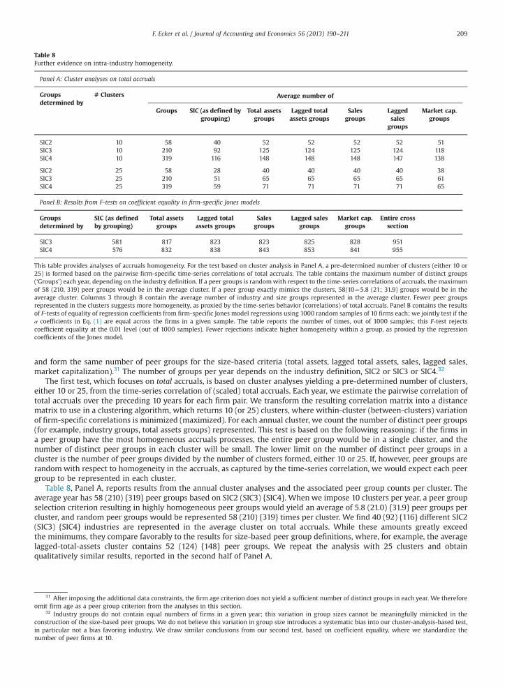
Table 8Further evidence on intra-industry homogeneity.
Panel A: Cluster analyses on total accruals
Groupsdetermined by
# Clusters Average number of
Groups SIC (as defined bygrouping)
Total assetsgroups
Lagged totalassets groups
Salesgroups
Laggedsales
groups
Market cap.groups
SIC2 10 58 40 52 52 52 52 51SIC3 10 210 92 125 124 125 124 118SIC4 10 319 116 148 148 148 147 138
SIC2 25 58 28 40 40 40 40 38SIC3 25 210 51 65 65 65 65 61SIC4 25 319 59 71 71 71 71 65
Panel B: Results from F-tests on coefficient equality in firm-specific Jones models
Groupsdetermined by
SIC (as definedby grouping)
Total assetsgroups
Lagged totalassets groups
Salesgroups
Lagged salesgroups
Market cap.groups
Entire crosssection
SIC3 581 817 823 823 825 828 951SIC4 576 832 838 843 853 841 955
This table provides analyses of accruals homogeneity. For the test based on cluster analysis in Panel A, a pre-determined number of clusters (either 10 or25) is formed based on the pairwise firm-specific time-series correlations of total accruals. The table contains the maximum number of distinct groups(‘Groups’) each year, depending on the industry definition. If a peer groups is randomwith respect to the time-series correlations of accruals, the maximumof 58 (210, 319) peer groups would be in the average cluster. If a peer group exactly mimics the clusters, 58/10¼5.8 (21; 31.9) groups would be in theaverage cluster. Columns 3 through 8 contain the average number of industry and size groups represented in the average cluster. Fewer peer groupsrepresented in the clusters suggests more homogeneity, as proxied by the time-series behavior (correlations) of total accruals. Panel B contains the resultsof F-tests of equality of regression coefficients from firm-specific Jones model regressions using 1000 random samples of 10 firms each; we jointly test if theα coefficients in Eq. (1) are equal across the firms in a given sample. The table reports the number of times, out of 1000 samples; this F-test rejectscoefficient equality at the 0.01 level (out of 1000 samples). Fewer rejections indicate higher homogeneity within a group, as proxied by the regressioncoefficients of the Jones model.
F. Ecker et al. / Journal of Accounting and Economics 56 (2013) 190–211 209
and form the same number of peer groups for the size-based criteria (total assets, lagged total assets, sales, lagged sales,market capitalization).31 The number of groups per year depends on the industry definition, SIC2 or SIC3 or SIC4.32
The first test, which focuses on total accruals, is based on cluster analyses yielding a pre-determined number of clusters,either 10 or 25, from the time-series correlation of (scaled) total accruals. Each year, we estimate the pairwise correlation oftotal accruals over the preceding 10 years for each firm pair. We transform the resulting correlation matrix into a distancematrix to use in a clustering algorithm, which returns 10 (or 25) clusters, where within-cluster (between-clusters) variationof firm-specific correlations is minimized (maximized). For each annual cluster, we count the number of distinct peer groups(for example, industry groups, total assets groups) represented. This test is based on the following reasoning: if the firms ina peer group have the most homogeneous accruals processes, the entire peer group would be in a single cluster, and thenumber of distinct peer groups in each cluster will be small. The lower limit on the number of distinct peer groups in acluster is the number of peer groups divided by the number of clusters formed, either 10 or 25. If, however, peer groups arerandomwith respect to homogeneity in the accruals, as captured by the time-series correlation, we would expect each peergroup to be represented in each cluster.
Table 8, Panel A, reports results from the annual cluster analyses and the associated peer group counts per cluster. Theaverage year has 58 (210) {319} peer groups based on SIC2 (SIC3) {SIC4}. When we impose 10 clusters per year, a peer groupselection criterion resulting in highly homogeneous peer groups would yield an average of 5.8 (21.0) {31.9} peer groups percluster, and random peer groups would be represented 58 (210) {319} times per cluster. We find 40 (92) {116} different SIC2(SIC3) {SIC4} industries are represented in the average cluster on total accruals. While these amounts greatly exceedthe minimums, they compare favorably to the results for size-based peer group definitions, where, for example, the averagelagged-total-assets cluster contains 52 (124) {148} peer groups. We repeat the analysis with 25 clusters and obtainqualitatively similar results, reported in the second half of Panel A.
31 After imposing the additional data constraints, the firm age criterion does not yield a sufficient number of distinct groups in each year. We thereforeomit firm age as a peer group criterion from the analyses in this section.
32 Industry groups do not contain equal numbers of firms in a given year; this variation in group sizes cannot be meaningfully mimicked in theconstruction of the size-based peer groups. We do not believe this variation in group size introduces a systematic bias into our cluster-analysis-based test,in particular not a bias favoring industry. We draw similar conclusions from our second test, based on coefficient equality, where we standardize thenumber of peer firms at 10.
F. Ecker et al. / Journal of Accounting and Economics 56 (2013) 190–211210
Our second test, which focuses on normal accruals, applies an F-test for coefficient equality to the firm-specific estimatedcoefficients in the Jones model. The hypothesis is that two firms with the same normal accruals generating process will havestatistically indistinguishable coefficients on the explanatory variables. For these tests, we require 10 firms per annualindustry cross section. In the most extreme case, requiring 10 firms per SIC4-year, the sample contains 109,473 firm-yearobservations. We first randomly draw 1000 industry-and-year pairs, and then 10 firms for each industry-year.The combination of our time-series and cross-sectional data requirements ensures a full panel of data for each sample;i.e., each draw consists of 10 firms with 10 annual observations to estimate firm-specific regressions. We estimate a firm-specific Jones model for each firm in a given sample over the 10 observations; using a joint F-test, we test whether the slopecoefficients α1, α2 and α3 in Eq. (1) are equal for all 10 firms.33
Panel B of Table 8 reports the proportion of samples (out of 1000) for which the test rejects coefficient equality at the0.01 level or better. The more homogeneous the accruals generating processes of the firms in a group, as captured bystatistically indistinguishable Jones model coefficients, the more likely the test will fail to reject equality of the coefficients.That is, smaller numbers in the table suggest a more homogeneous normal accruals generating process within groups.Across the three industry definitions, we find that F-test rejects coefficient equality for 576–641 of the 1000 industry groups,or approximately 58–64%. This rejection rate is both high in absolute terms and substantially lower than the rejection ratesfor the size-based peer group definitions, averaging approximately 82.5% or higher.
To summarize, we perform two tests of homogeneity in the total accruals generating process and the normal accrualsgenerating process to supplement our analysis of how estimation sample selection criteria affect the power to detectabnormal accruals. The first test defines homogeneity in terms of the time-series correlation of total accruals and the secondtest defines homogeneity in terms of equality of firm-specific regression coefficients from a Jones model. Both tests confirmgreater homogeneity of industry-based estimation samples, with respect to the accruals attributes we consider, relativeto size-based estimation samples. Industry-based estimation samples should therefore provide the most efficient cross-sectional estimates of normal accruals, subject to concerns about (possibly considerable) sample attrition. In addition,industry definitions of normal accruals seem far from perfect, confirming previous research, e.g., Bernard and Skinner, 1996;Brickley and Zimmerman, 2010; Dopuch et al., 2012, suggesting considerable accruals heterogeneity among firms in thesame industry.
7. Summary and conclusions
We examine the ability to detect discretionary accruals using several variants and extensions of the Jones (1991) modelof discretionary accruals and estimation samples based on two alternative indicators of similarity: industry membership(industry peers) and size (size peers). Our examination is motivated by the practical problem of sample attrition whenestimation samples are based on industry membership, particularly the SIC4 industry definition, and particularly for non-U.S. data.
Our main finding is that estimation samples based on similarity in size as measured by lagged total assets perform atleast as well as industry membership-based estimation samples, and often better, in detecting both seeded discretionaryaccruals and observed discretionary accruals (as proxied by the existence of a restatement or an Accounting and AuditingEnforcement Release). The superior discretionary accruals detection power of lagged asset-based estimation samples appliesto both U.S. data and non-U.S. data. For non-U.S. samples not constrained by the availability of industry peers, lagged asset-based estimation sample detection rates are similar to the detection rates observed for samples where we can perform acontrolled comparison of detection rates for industry-based peers and lagged asset-based peers.
We provide evidence of a tradeoff between increasing explanatory power of normal accruals models and increasing detectionpower for abnormal or discretionary accruals. While both size-based and industry-based estimation samples produce reasonableexplanatory power in estimating normal accruals, the industry-based samples achieve higher explanatory power. This result iscorroborated by additional analyses showing industry-based samples are characterized by normal accruals with greater congruitythan are size-based samples, although neither sample selection criterion yields normal accruals that are wholly or evensubstantially congruent. In contrast, size-based estimation samples, in particular, samples based on similarity in lagged totalassets, often yield higher detection rates for abnormal or discretionary accruals. Viewed as awhole, these results suggest the greaterdetection power of the size-based estimation samples is due to the greater stability of the accruals model regression estimatedusing size-based samples, as compared to using industry-based samples, and this greater stability comes at the cost of lowerexplanatory power.
Defining estimation samples (peer firms) based on similarity in lagged assets instead of industry membership hassubstantial practical value in estimating discretionary accruals models because application of the size-based criterionimposes no incremental sample loss, beyond the sample losses resulting from estimating the variables in the models. ForU.S. data, this means avoiding sample attrition of anywhere from 1–3% (SIC2 definitions) to 22–30% (SIC4 definitions).The benefits, in terms of increased sample sizes, are much greater for non-U.S. data, where using lagged assets instead ofindustry membership to identify estimation samples avoids sample attrition ranging from 32% to 93% (depending onindustry definitions and weighting schemes).
33 We do not impose α1¼α2¼α3 for each firm.
F. Ecker et al. / Journal of Accounting and Economics 56 (2013) 190–211 211
We believe our finding concerning the discretionary accruals detection power of lagged asset-based estimation samplesis important both in the U.S. context and in the non-U.S. context. For both settings we show that using lagged asset-basedsamples rather than industry-based samples to estimate discretionary accruals models increases sample sizes, oftensubstantially, and generally results in equal or better detection of discretionary accruals. The overall effect is more dramaticfor non-U.S. settings and more valuable, because in those settings, entire countries dropped in an industry-based estimationsample design can be retained in a size-based estimation sample design.
References
Albuquerque, A., 2009. Peer firms in relative performance evaluation. Journal of Accounting and Economics 48, 69–89.Bernard, V., Skinner, D., 1996. What motivates managers’ choice of discretionary accruals? Journal of Accounting and Economics 22, 313–325.Brickley, J., Zimmerman, J., 2010. Corporate governance myths: comments on Armstrong, Guay and Weber. Journal of Accounting and Economics 50,
235–245.Dechow, P., Ge, W., Larson, C., Sloan, R., 2011. Predicting material accounting misstatements. Contemporary Accounting Research 28, 17–82.Dechow, P., Sloan, R., Sweeney, A., 1995. Detecting discretionary accruals. The Accounting Review 70, 193–225.Dopuch, N., Mashruwala, R., Seethamraju, C., Zach, T., 2012. The impact of a heterogeneous accrual-generating process on empirical accrual models. Journal
of Accounting, Auditing and Finance 27, 386–411.Healy, P., 1985. The effect of bonus schemes on accounting decisions. Journal of Accounting and Economics 7, 85–107.Hennes, K., Leone, A., Miller, B., 2008. The importance of distinguishing errors from irregularities in restatement research: the case of restatements and
CEO/CFO turnover. The Accounting Review 83, 1487–1519.Jones, J., 1991. Earnings management during import relief investigations. Journal of Accounting Research 29, 193–228.Kothari, S.P., Leone, A., Wasley, C., 2005. Performance matched discretionary accruals measures. Journal of Accounting and Economics 39, 163–197.Larcker, D., Richardson, S., 2004. Fees paid to audit firms, accrual choices, and corporate governance. Journal of Accounting Research 42 (3), 625–658.