Embed Size (px)
Citation preview

Discrete Vector Potential Representation of a Divergence-Free Vector Field in Three-Dimensional Domains: Numerical Analysis of a Model ProblemAuthor(s): Francois DuboisSource: SIAM Journal on Numerical Analysis, Vol. 27, No. 5 (Oct., 1990), pp. 1103-1141Published by: Society for Industrial and Applied MathematicsStable URL: http://www.jstor.org/stable/2157797 .
Accessed: 12/06/2014 22:40
Your use of the JSTOR archive indicates your acceptance of the Terms & Conditions of Use, available at .http://www.jstor.org/page/info/about/policies/terms.jsp
.JSTOR is a not-for-profit service that helps scholars, researchers, and students discover, use, and build upon a wide range ofcontent in a trusted digital archive. We use information technology and tools to increase productivity and facilitate new formsof scholarship. For more information about JSTOR, please contact [email protected].
.
Society for Industrial and Applied Mathematics is collaborating with JSTOR to digitize, preserve and extendaccess to SIAM Journal on Numerical Analysis.
http://www.jstor.org
This content downloaded from 188.72.126.41 on Thu, 12 Jun 2014 22:40:02 PMAll use subject to JSTOR Terms and Conditions

SIAM J. NUMER. ANAL. ? 1990 Society for Industrial and Applied Mathematics Vol. 27, No. 5, pp. 1103-1141, October 1990 001
DISCRETE VECTOR POTENTIAL REPRESENTATION OF A DIVERGENCE- FREE VECTOR FIELD IN THREE-DIMENSIONAL DOMAINS:
NUMERICAL ANALYSIS OF A MODEL PROBLEM*
FRANCQOIS DUBOISt
Abstract. For the representation of a divergence-free vector field defined on a bounded simply connected domain of R 3 with a smooth boundary by its curl and its normal component on the boundary, a mixed formulation also involving a vector potential is proposed. The vector fields are discretized with help of curved finite elements that are conforming in H(div) or H(curl). A discrete gauge condition is proposed to assume the uniqueness of the stream function. Optimal error estimates are derived, and a numerical experiment is presented.
Key words. mixed finite elements, curved boundaries, discrete gauge condition
AMS(MOS) subject classification. 65N30
1. Introduction. When we study numerical fluid dynamics, an important task is the discretization of vector fields u that are divergence-free (or solenoidal):
(1.1) div u = 0
with u defined on a domain Ql of LR3. The major field of application is incompressible hydrodynamics (Temam [43]); replacing u by the mass flux, we find that (1.1) is also important in stationary compressible aerodynamics (Courant and Friedrichs [15]). A conforming or nonconforming discretization that respects (1.1) is difficult to obtain with the finite-element method (Hecht [29], Gustafson and Hartman [28]). On the other hand, a natural way of satisfying (1.1) exactly is to represent u in terms of a vector potential T:
(1.2) u = curl T
but the uniqueness of W is never assumed and a gauge condition must be added. A classical way is to prescribe the Coulomb gauge (e.g., Jackson [30]):
(1.3) div TI=0.
Moreover, different choices of the boundary conditions for t are possible. The studies of Bernardi [9] and Bendali, Dominguez, and Gallic [6] have given existence and uniqueness results. Practically, the stream function is just a tool for representing the field u and must be computed easily if we give some constraints on this field. In this paper, we choose to fix the vorticity o and the mass inflow g over the entire boundary:
(1.4) curlu-= inQf,
(1.5) u-n=g ondQf.
We remark that if (1.2) and (1.5) are satisfied, then the average of the mass inflow g on each component of the boundary of Ql is null. This fact precludes flow problems with sinks and sources.
* Received by the editors October 14, 1987; accepted for publication (in revised form) August 8, 1989. t Ecole Polytechnique, Centre de Mathematiques Appliquees, F-91128 Palaiseau Cedex, France. Present
address, Aerospatiale, Division Systemes Strategiques et Spatiaux, S/DT/MI, BP 96, F-78133 Les Mureaux Cedex, France.
1103
This content downloaded from 188.72.126.41 on Thu, 12 Jun 2014 22:40:02 PMAll use subject to JSTOR Terms and Conditions

1104 FRAN4FOIS DUBOIS
With these assumptions we restrict ourselves to a simple problem. More sophisti- cated models, for example, are the Stokes and Navier-Stokes equations in (*, t), formulation (Girault and Raviart [26]), and the potential isentropic equations of transonic flow (Courant and Friedrichs [15]). However, even in the linear case of the Stokes problem, the numerical analysis of the three-dimensional case is difficult (Nedelec [38]).
In ? 2, after recalling classical results on vector fields, we split the linear problem into a homogeneous problem in Ql (g = 0) and a problem on the boundary of f (g $ 0). Then a concrete construction method of i from the only data (w, g) is presented. In the discretized problem, the compatibility between these two subproblems requires that the discrete field 4h have a tangential component on each point of the boundary. Thus in ? 3 we develop curved finite elements conforming in the spaces H(div) and H(curl), which coincide in the straight case with the vectorial finite elements of degree 1 introduced by Nedelec [37]. Then we derive optimal interpolation errors. Section 4 treats the approximation of the homogeneous problem. The major difficulty is the definition of a "good" linear space, which guarantees that the discrete potential is unique. Therefore, we adapt the discrete gauge communicated by Roux [41] to the case of arbitrary simply connected domains in lR3. Then we formulate the discrete problem and obtain the error estimate between the velocity field and its approximation. By linearity, ? 5 treats only the approximation of a harmonic vector field (o = 0). The boundary finite elements of Nedelec [34] and Bendali [3], [5] are adapted to H(curl), and a discrete gauge is added to assume the uniqueness of the tangential component of the discrete stream function. Then the error estimation is established.
1.1. Hypotheses and notation. We define fl as a connected bounded domain of R3 with a regular boundary df = r, and Fj(j = 0, 1, * - *, NF) as the connected com- ponents of F. We assume that Fo is the boundary of the unbounded component of R3\fl. Classically (e.g., Nedelec [34], [35]), the structure of regular (of C2 class) manifold with boundary ensures the existence of (p + 1) open sets fOl,Q f,Qp of R3 covering Q:
fl 0u_ (j i- i ) -
Moreover, the p last f)i's cover the boundary:
Fc u fi I rA f)o = 0.
The local charts )ui are compatible diffeomorphisms of class C2:
(1.6) Hti: Qli _
(]_-1, 1 [)3, i = O , * p,
(1.7) 1Vi|,nn,= An,nn i,j=0,1, *,p
and fl is supposed to be locally on one side of its boundary:
(1.8) ki(rFn Qif) = (]-1, 1[)2 X (0), i = 1, * , (1.9) A(fmn fii) = (]-1, 1[)2X]0, 1[, i= 1, ,p.
We finish this geometrical description by introducing the normal projector on the boundary (e.g., De Rham [16]).
PROPOSITION 1.1. There exists 8 > 0 and a neighborhood U, of r:
U8={xc R3, dist(x, F)?}
This content downloaded from 188.72.126.41 on Thu, 12 Jun 2014 22:40:02 PMAll use subject to JSTOR Terms and Conditions

DISCRETE VECTOR POTENTIAL IN THREE DIMENSIONS 1105
such that each point x of U8 admits a unique projection PrX on F:
VxE U8 3! y = Prx E r, xy normal to r. Now we make one hypothesis on the algebraic topology of fl, and introduce some
notation relating to boundary operators. The domain fl is supposed to have NH holes (if NH = 0, fl is simply connected) and it is possible to find NH regular surfaces Ik
such that (Q\(U k-H1 Ik)) is a simply connected domain of Rl (Foais and Temam [22]). The following operators on the manifold F are defined in Choquet-Bruhat [13], for example:
* Surface gradient Vrw and surface curl, curliw, of a scalar function defined on r: curlrw = Vfw x n with n the external normal to F.
* Surface curl, curlr t, and surface divergence divr t of a tangent vectorial function defined on F. We have divr t = curlr (n x t). Finally, the Laplace-Beltrami operator Ar satisfies
-Ar,w = curlr (curlr w) = -divr (Vrw).
By duality these operators are also defined for scalar (T) or vectorial (U) distributions on F:
(VrT, g)r =-(T, divr gr,
(curlr T, g)r = (T, curls g)r,
(curls U, w)r = (U, curlr W)r,
(divr U, w)r[ = (U, V r w)r[
In this notation, the duality product ( *, - )r of two vectors is the scalar product according to the metric gij on the manifold (e.g., Choquet-Bruhat [13]):
(U, Or = ; ( Ui, giAXj)- iQj
* More generally, the scalar product between two vectors 'p, * defined in fl, or two tangent vectors on r, is denoted by sp -I* (or (p, I) when - is used for the image A u of a vector u by a mapping A); the tangential component of r of a vector p is
1l1p =nx (pxn) = (nx p) xn,
and we have a Green formula for regular vector fields:
(1.10) I - curl Tdx={ curlhp - IFdx+{ (p x n) - I dy.
Moreover, Span (ul, * - *, u,,) is the linear space of all the linear combinations of the vectors ul, * * *, un and tA is the transpose of a matrix A.
2. The continuous problem. We first recall the definitions of some classical Sobolev spaces. Then the major results concerning the decomposition of vector fields reviewed in Bendali, Dominguez, and Gallic [6] and also established by Friedrichs [23], Foias and Temam [22], and Georgescu [24] are given. We also propose a mixed formulation in the variables (u, *) to compute both the velocity field u and the potential f in the particular case of homogeneous constraints on u:
(2.1) divu=0 nfl
(2.2) u * n =O ondQf.
This content downloaded from 188.72.126.41 on Thu, 12 Jun 2014 22:40:02 PMAll use subject to JSTOR Terms and Conditions

1106 FRAN?OIS DUBOIS
In the nonhomogeneous case, i.e., if
(2.3) u - n= g onafl,
we first consider a boundary problem for which we give a mixed formulation. Then the extension theorem of J.L. Lions (Lions and Magenes [32]) allows a theoretical approach to computing the vector potential * with
(2.4) u curl ,
if u satisfies both (2.1) and (2.3).
2.1. Some Hilbert spaces. The Sobolev spaces L2(fQ), H'(fl), H2(fQl) are Hilbert spaces with their natural norms 11 110JI, 11 |1Qi, and 11 112,Q, respectively (e.g., Adams [1]). We also set
Hl(f) ={w c H1(f), w1rv=0},
L2(fl)={ 2(fl),{wd 0} Lo(Q w C L2QA wdx-0}
Following Duvaut and Lions [20], we define
H(div, fQ) = {v c (L2(fQ))3, div v c L2(Q)},
H(curl, fQ) = {ep c (L2(fl))3, curl sp c (L2(Q))3},
and the associated norms 11 IIH(di,) and 11 IIH(cur1) We also consider vector fields that are normal on the boundary:
H?(curl, fQ) = {p c H(curl, r), p x nl I0}. The classical spaces H'(F) (s real) of scalar functions (and distributions) defined on the Q-boundary are equipped with their natural norms 11 lsFr The duality product between H-'12(F) and H112(F) is denoted by (, *)r, and THS(F) are tangent vector fields on r (e.g., [4]):
THs(F) -{ c (Hs(r))3, M n - 0}.
Consider now some particular spaces useful in this paper. DEFINITION 2.1.
W2(fQ) ={p c (H1(Q))3, curl 0p C(Hl(Q))3} M(F) = {g distribution on F, (g, 1)I,- = 0, V *i * 0, N-1.
The notation introduced above for the norms of scalar fields will also be used for the norms of the corresponding vector fields when there is no ambiguity.
PROPOSITION 2.1. The norm
jjlp II W2(n)-(112 n+curl 112,n )1/2
defines on W2(fQ) a structure of Hilbert space.
2.2. Decomposition of vector fields. In this section, we recall general results on vector fields defined on a regular bounded domain Ql of R . We refer to Bendali, Dominguez, and Gallic [6] and to their included references for the results.
DEFINITION 2.2. The two sets
XT(f) -{vc (L 2(fl))3, div v c L2(fQ), curl v C (L2(fQ))3, v n c H1/2()
XN (Q) = {v C (L2 (Q))3, div v c L2(Q), curl v c (L2(Q))3, v x n c TH /2(r)},
are Hilbert spaces equipped with their natural norms 11 1IT and 11 11N, respectively. THEOREM 2.1. The vectorspacesXT(fl) andXN(fl) are equal to (H1(fl))3 algebrai-
cally and topologically.
This content downloaded from 188.72.126.41 on Thu, 12 Jun 2014 22:40:02 PMAll use subject to JSTOR Terms and Conditions
DISCRETE VECTOR POTENTIAL IN THREE DIMENSIONS 1107
We introduce tangential and normal harmonic vector fields, related to topological invariants of Ql.
DEFINITION 2.3.
HT(fl) = {v (L2(Q))3, div v = 0, curl v =0, v - nlr = 0},
HN(n) = {ve (L2(fQ))3, div v = 0, curl v =0, v x nlr = 0}. THEOREM 2.2. We have dim HT(fQ) = NH, dim HN(n) = Nr. There exists a unique
basis (OT)1?l?N, of HT(%) (respectively, (O7)1i-jNT of HN(fQ)) such that J O7k - n dy = 8ikfor all i, k= 1, , NH (respectively, Jr, I - n dy = 8j, for j, = 1, , Nr).
PROPOSITION 2.2. The orthogonal projectors PT and PN, PT: XT(fl) - HT(fl), and PN XN(fl) - HN(fQ) with respect to the associated scalar products admit the following expressions:
(2.5) PTV=Z ({ . iTdx)oT,
(2.6) PNV= E ( V *7jdx)07 j=l Ql
for some basis oT of HT(fQ) (respectively, o7 of HN(fQ)). Thus (2.5), (2.6) define PT and PN as orthogonal projectors from (L2(fQ))3 onto HT(fl) and HN(%), respectively.
Proof of Proposition 2.2. The auxiliary bases oT and o7 are constructed explicitly by Foias and Temam [22], Dominguez [17], and Bendali and Gallic [7] as gradients of some harmonic functions defined on (fl\U;N= 1i) and on fQ, respectively. The end of the proof is clear. O
PROPOSITION 2.3. Let v be a solenoidal vectorfield (div v = 0) in (H1(ft))3. We have
(2.7) PNV= (f v n dy) 0,
(2-8) PTV = (V n d) OT if v nlr = .
Proof of Proposition 2.3. We prove only (2.7) since the proof of (2.8) is similar. Following Bendali and Gallic [7], let frj be the solution of
qj=0 fi,
4ij= 0 Fo,
4j =% Fig i i = 1, ... 9 Nr,,
We set ON = VqIj and integrate by parts. We have
{vO 70j dx= T v*nfjdy
if div v= 0. Thus (2.7) holds. O THEOREM 2.3. The mappings
XT (f) V-IVI T = (II curl VII| 2Q + || div VII| 2Q + 11 PTVII| 2Q + IV * n 112 /2vr)
XN (f) 3 V|-41VIN = (II curl Vi| i Q + || div Vi| iQ + 11 PNVII 2Q + liv Xln 1/2,r)
are norms on XT(fQ) and XN(fQ) that are equivalent to the Hl(fl) norm. DEFINITION AND PROPOSITION 2.4. We set
W1(fQ)={PE (H'(fQ))3,div p =0, pXnIn=0, 09 ndy=0,Vj=1, Nr-
This content downloaded from 188.72.126.41 on Thu, 12 Jun 2014 22:40:02 PMAll use subject to JSTOR Terms and Conditions

1108 FRANQOIS DUBOIS
Then the mapping W1'() > p-*IIcurl pII o,n c R is a norm on W1(fQ) that is equivalent to the H1 norm.
Proof. The proof is a direct consequence of Proposition 2.3 and Theorem 2.3. 0
THEOREM 2.4 (Decomposition of vector fields). For u given in (L2(fQ))3, we have the following decompositions:
(2.9) (i) u =Vw + curl p + (uOTdx)0T
with unique (w, up) verifying
(2.10) w E Hl(Q) nL L20(fl) WI (Q).
(2.11) (ii) u = VP + curl ? + E (u. uodx) 7j
with unique (p, j) verifying
(2.12)p 22 E (Hl(fl))3, div J=0, *nlrp= 0, PT4 =0.
Moreover, if u belongs to (Hm(f))3 (m ?0) then w, p, p, ij belong to Hm+l). The decomposition (2.9) (respectively, (2.11)) of the field u is into three orthogonal
components of the type Vw (respectively, Vp), plus curl sp (respectively, curl I'), plus some vector lying in HT(fQ) (respectively, HN(fQ)). However the decomposition (2.5) (respectively, (2.6)) of the projector PT (respectively, PN) is not split into orthogonal components in L2(fQ) and the auxiliary vectors OT (respectively, P7) introduced at Proposition 2.2 constitute the dual basis of the OT (respectively, o0N).
The results of Theorem 2.4 have been used by El Dabaghi and Pironneau in their numerical work [21].
2.3. Mixed formulation of the homogeneous problem. If a vector field u admits a representation of the type u = curl up, we clearly have
(2.13) div u = 0,
but we also have constraints on the normal component. LEMMA 2.1. Let up be in the space W1(fl). We have in the space H112(F): curl up n =
divr up x n = curlr Hp. Proof of Lemma 2.1. Consider a regular function w on F and a lifting of w on Ql
also denoted by w. We have
(curl hp - n, w)r={ div (w curl hp) dx Vw- curl hp dx
=-(V w, sp x n)r = (divr sp x n, w)r
by definition of the operator divr. Moreover, for an arbitrary tangent vector field t on F, we have curlr (n x t) = divr, (e.g., Choquet-Bruhat [13]). U
PROPOSITION 2.5 (Foias and Temam [22]). Let u c (L2(fQ))3 and J E H(curl, Q), satisfying u = curl J. Then we have
(2.14) PNU=0.
If u E (H1(fl))3 and J E W2(fQ), then this condition can be written as r, u- n dy = 0 for
This content downloaded from 188.72.126.41 on Thu, 12 Jun 2014 22:40:02 PMAll use subject to JSTOR Terms and Conditions

DISCRETE VECTOR POTENTIAL IN THREE DIMENSIONS 1109
Proof of Proposition 2.5. From Proposition 2.2 (see (2.6)) we have
f u *o dx = L curl 4 o7 dx
={| 4 * curl Oj dx-f *(n x 7) dy
because 07 E HN (fQ). Then PNU = 0. The end of the proof is a consequence of Proposi- tion 2.3. Directly, from (2.12) and Lemma 2.1, we have u n = divr(I x n) on dQl and we integrate this function on the component Fi. ?
Now we suppose that hypotheses (2.13) and (2.14) are true. We emphasize that, in practice, (2.14) precludes flow problems with sinks and sources. In the rest of this section we present a way to construct a vector potential t. We begin with the simple case u - n-O on F.
THEOREM 2.5. The mixed problem
U E (L 2(Q))3, * E W, (Q),
(2.15) {u- v dx -J curl*- v dx=O Vve (L2(fl))3,
u - curl ,p dx ={ - *p dx Vp E W1(f)
admits, for o given in (H1(fl)')3, a unique solution that satisfies div u = 0. Moreover, if t E (L2(fQ))3 such that (2.13), (2.14) is satisfied, u belongs to (H1(fQ))3 and we have
(2.16) u*n=O F,
(2.17) curlu=t fQ,
(2.18) IIuIIo,?- CI I(IO,c
for some constant C. Proof of Theorem 2.5. * The existence and uniqueness are consequences of the Brezzi-Babuska condition
(Brezzi [11], Babuska [2]), which is satisfied because on the one hand
(L2(fl))6 3 (U, V) u *{ v dx C R is coercive,
and on the other hand
Sup I curl -vdxlcurl EpIIO,Q_ CI,n
(we choose v = -curl up to obtain the first inequality and we refer to Proposition 2.4 for the second). The first equation implies u = curl 4 and therefore div u = 0.
* If o belongs to (L2(fQ))3 and satisfies both div o =O and PNto =O, Theorem 2.4(ii) shows that we can write
(2.19) t = Vp +curl J.
Since the scalar p belongs to H (fQ), we have p = 0. Besides, we also have J C (H (Q))3, div J= 0, J = nlr0= . We demonstrate now that u -J belongs to HT(ft), i.e., that the
This content downloaded from 188.72.126.41 on Thu, 12 Jun 2014 22:40:02 PMAll use subject to JSTOR Terms and Conditions

o10 FRANQOIS DUBOIS
pair (w, sp) of the decomposition of u-J, by means of Theorem 2.4(i), is equal to zero. We have
f(u-J)* Vwdx= (u-J) - nwdy= u- nwdy=0,
f(u-J) curl hp dx={ u curl Sp dx - curl J -p dx because sp x n = 0
due to (2.15) and (2.19).
Thus u E (H1(f1))3 and (2.16)-(2.17) are clear. We choose sp = j in the second equation of (2.15). From Proposition 2.4, we deduce 0 U 1 Ik IIo,QII' iio,Q C C IkZIIo,n IIcurl 'pIIO'n, which corresponds to (2.18). 0
2.4. Mixed formulation of the boundary problem. In this section we suppose that the boundary F is connected (if it is not, we just have to replace the function spaces by their (Nr+ 1) copies for the different connected components of F). We recall first general results on scalar and tangent vector fields on F.
THEOREM 2.6. Let s be a real number, and let g be an element of Hs(Fn M(F)). The problem -ArO = g admits a unique solution 0 E HS?2(F) n M(F) satisfying 11 0 11 s+2,r-
C (s) 11 g 11 S,r for some constant C (s) independent of g. Proof. See, e.g., De Rham [16] or Treves [44] for the proof. O DEFINITION 2.5. We denote by Y(F) the space of tangent vector fields 0 on F
with curlr 0 = divr O = 0. We define W112(F) by
W12(F) - {ii TH1"2(F), divr, i = 0, *Ody=O, VO c Y(F)}.
THEOREM 2.7 (Georgescu [24], Treves [441). The space Y(F) is finite dimensional and there exists some integer r such that dim Y(F) = 2r (F is diffeomorphic to the torus with r handles). Moreover, for s a given real number, the mapping
(HS+l(F) nM(F))2x Y(F) 3 (p, w, 0) -q = Vrp +curlr w + 0 c THs(F)
defines an algebraic and topologic isomorphism. Those important results allow us to derive a Poincare-type inequality in the space
w1/2(F). PROPOSITION 2.6. The mapping W1/2 3 q4curll 11 -I/ -2r E R is a norm on W"/2(F)
that is equivalent to the norm induced by TH1/2(F):
3 C >O Vq} E W12 (F), ll ll l/2,F-' C llcurl,a ll -1/2,r-
Proof of Proposition 2.6. The field M E TH112(F) admits a decomposition given in Theorem 2.7 with p, w in H3/2(F) n M(F) and 0 E Y(F). Clearly, we have ArP = divr Mq =
0, and then p = 0, thanks to Theorem 2.6. Moreover, when we integrate M against 0, we have Jr- - 0 dy = Jr 0 0 dy = 0, so 0 = 0. Then
l1ii1/2,r= IIcurlr W 1|1/2,rF lWll3/2,F < CIIcurlr1 71I-1/2,r
due to (2.20), Theorem 2.6, and curlr aq H-"/2(F), with
(2.20) -Arw = curlr vj. E
Now suppose that the mass flux g across the boundary is given in M(F). We have seen (Proposition 2.5) that the component g of the vector potential satisfies
(2.21) curlr = g.
This content downloaded from 188.72.126.41 on Thu, 12 Jun 2014 22:40:02 PMAll use subject to JSTOR Terms and Conditions

DISCRETE VECTOR POTENTIAL IN THREE DIMENSIONS 1111
If we choose 9 in W1"2(F), we add the continuous gauge condition
(2.22) divr- = 0
and t can therefore be rewritten as
(2.23) t = curlr 0.
We now propose a mixed formulation of the problem (2.21)-(2.23). PROPOSITION 2.7. Let g be in H 112(F) n M(F). The mixed problem
e w1'2(F), 0 E L2(F) n M(F),
(2.24) {. ddy- -{0 curlrw dy=O V W"2(F),
curlr gw dy = (g, w)rp Vw E L2(F) n M(F)
admits a unique solution (g, 0) E W1/2 x (L2 n M) satisfying (2.21), (2.23), 0 E H3/2(F), and
(2.25 ) 1 /2,r- _ C 11 g 1 /2,F
Moreover, if g E H/2(F), we have 0 E H5/2(F) and g e TH312(F). Proof of Proposition 2.7. * Following Raviart and Thomas [40], we clearly see that the pair (0, curlr 0),
with 0 E M(F) the solution of -Art = g, is the solution of (2.24) because (w, curlr ii)r = (curlr w, )r for w E H1/2 and q E TH112. The uniqueness is established by linearity: if g = 0, the second equation shows that curlr t = 0, then = 0 (Proposition 2.6). Further- more, let p, in H2(F) n M(F), be the solution of -rp = 0. If we set M = curlr p, then
W W '2(F). If we use this function in the first equation of (2.24), we find Jr 02 dy = 0. The estimation (2.25) is then a simple consequence of Proposition 2.6.
* Relation (2.21) holds in the sense of distributions because both curl1r and g are equal if they are applied to functions of L2(F) n M(F) or to constant functions.
* If g belongs to H/2(F), the regularity of 0 is clear. O
2.5. A global result. We consider a velocity field in (H'(Q))3 satisfying
(2.26) div u = O Q,
(2.27) {u n dy = O on Fj, j = O, 1,9 * * Nr
and we suppose that both o and g satisfy
(2.28) curl u = X f,
(2.29) u*n=g F.
In Proposition 2.8 we propose a way to "compute" without ambiguity a vector potential * of u:
(2.30) u = curl l Q.
First we recall a theorem of J. L. Lions (right inverse of the trace operator). THEOREM 2.8 (e.g., Lions and Magenes [32]). The trace mapping yo, defined by
yo = o I'(9 8p/dnlI) if p is regular, can be extendedfrom H2(Q) onto H3/2(r) x H"/2(r)
This content downloaded from 188.72.126.41 on Thu, 12 Jun 2014 22:40:02 PMAll use subject to JSTOR Terms and Conditions

1112 FRANCOIS DUBOIS
and admits a continuous inverse R, from H3/2(r) x H1/2(r) to H2():H3/2(r) x H"/2(r) 3 qH-*4q c H2(fl)
y,(Rq) = q Vq c H312 x H12
3 C > 09 Rq 112 H < C || q | /3H2 x H1!2
PROPOSITION 2.8. Let u be given in (H1(fl))3 by (2.26)-(2.29). There exists a continuous vector potential * that satisfies (2.30) and defines a continuous mapping (HI(l)) 3 _W2(fQ) computable without any use of the harmonicfunctions belonging to the spaces HT(fl) and HN(Q).
Proof of Proposition 2.8. * Consider first the boundary equation (2.29). From Proposition 2.7 there exists
some t c TH3/2(r) verifying (2.21). Each component ei of t belongs to H3/2(F) and, by Theorem 2.8, the vector field g defined on Q by its components j, j = R(ei, 0) satisfies curlr 11; = g and
11 2I <I2Q C11911312,Fc C 11 11 /2,F
* Second, the mixed problem
zc (L 2(Q))3, X WI (Ql),
z v dx- curl X v dx Vv c (L2(fQ))3,
z curlhpdx={ (w-curlcurl ).pdx Vbp Wl(fQ)
admits (according to Theorem 2.5) a solution (z, X) satisfying z = curl x- curl z= w-curl(curl ) in Ql, z-n=0 on r, and iIXIIw2'-C(IIWIIO,Q+IIII2,) thanks to (2.18) and Proposition 2.4. By uniqueness of z, we have z = u - curl 4 in Q, so X = X + g solves the problem. O
We end this section with a general result on harmonic vector fields. PROPOSITION 2.9. Let g be in H /2 (r) n M(r). The problem
divu=0 Q,
curl u = O f, (2.31)
u - n=g F,
PNU = 0
has a unique solution u c H(div, fl) that satisfies
(2-32) IJUIIO,n ' C ||g||-112,F
for some constant C independent of g. Proof of Proposition 2.9. * Following Temam [43], the auxiliary problem
-A4 = O , -= g F
defines 4 c Hl(m) n L2(f) and the continuity of g+-4: IV4II0&' C11g91+112 is classical. If we take u = V4, the existence of u satisfying (2.31)-(2.32) is established.
* Uniqueness is a direct consequence of Theorem 2.2. 0
This content downloaded from 188.72.126.41 on Thu, 12 Jun 2014 22:40:02 PMAll use subject to JSTOR Terms and Conditions

DISCRETE VECTOR POTENTIAL IN THREE DIMENSIONS 1113
3. Vectorial curved finite elements in R3. We have seen in the study of the con- tinuous problem that the representation of a divergence-free vector field u by means of a vector potential * leads to the internal and boundary equations curl * = u in Qk and curlr TIi = u * n on F. To discretize the field *, we choose finite elements conforming in the space H(curl, fl) such that the boundary F is exactly covered by the triangulation faces. Here we introduce two different curved finite elements of degree 1 that are conforming in the spaces H(div, fl) and H(curl, fl) and are a natural generalization of Nedelec's tetrahedrons [37]. Then we show that for v in H(div, fQ) (respectively, p in W2(fQ)) the interpolation error in the associated discrete space Vh (fQ) (respectively, Wh(fl)) is of optimal order. In what follows we construct a triangulation Sh covering exactly the domain fl. We denote by 3-hla0 the subset of -h formed by elements K such that the intersection Kn afi is not void.
3.1. Definition of curvilinear tetrahedrons. DEFINITION 3.1. Let K be the "unity tetrahedron":
K ={(x1,x2,x3)EDR3,xi-O, i= 1,2,3,xI+x2+x3 1}.
A curvilinear tetrahedron is defined by the range of K by a regular (class (C2) one-to-one function F:
(3.1) K Xx = F(x E K.
Practically, either K is an internal element of the triangulation and F is assumed to be a linear mapping (this hypothesis will be implicit in what follows), or K has at least one point on the boundary.
When the latter is true, four cases can occur: (i) Kn afi is an edge of the tetrahedron. (ii) Kn afi is a face of the tetrahedron. (iii) Kn afi is reduced to one point. (iv) Kn afi contains at least two faces of K.
In case (iii), F is also chosen linear, and case (iv) can be eliminated by a refinement of the mesh. We focus now on cases (i) and (ii) (Fig. 3.1).
Hypothesis 3.1. We assume that the triangulation 3h is sufficiently refined (i.e., h sufficiently small) to be sure that the orthogonal projection Pr is well defined on YhIa0
(Proposition 1.1). DEFINITION 3.2. (i) Assume that exactly two vertices A1, A2 of K belong to the
setr nF , defined in (1.6)-(1.8). The curved edge A1A2 is defined as Pr([AIA2]), where [AIA2] is the straight line between these two points.
Case (i) Case (ii)
FIG. 3.1. Intersection of a curvilinear tetrahedron with the boundary.
This content downloaded from 188.72.126.41 on Thu, 12 Jun 2014 22:40:02 PMAll use subject to JSTOR Terms and Conditions

1114 FRAN4OIS DUBOIS
(ii) If afl contains three vertices A1, A2, A3 of K, the curved face A1A2A3 is exactly Py([A1A2A3]), where [A1A2A3] is the corresponding plane face.
We can now describe the choice that we are making for the curved elements K of _9han-
DEFINITION 3.3. If x is a point of the unity tetrahedron K, we denote by Aj(j 1, -, 4) its barycentric coordinates.
(i) If K contains a curved edge 2, we set
(3.2) F(x) = (1 -A3-A4)PF (AlA+A2A2 +A3A3+A4A4.
(ii) If a curved face A1A2A3 is included in dQ, we set
(3.3) F(^A) = (1 -A4)Pl 'A'A1+A2A2+A3A3 +A4A4 (3.3)FGi~)(1~A4PvI\ A1+A2+A3 /
(see Fig. 3.2). This type of definition was first proposed by Zlamal [45], [46], studied by Scott
[42], and generalized by Lenoir [31]. Geometrically we first write a current point x of the straight tetrahedron [A1A2A3A4] as a barycentre of one point y on the edge [A1A2] (case (i), p =2) or on the face [A1A2A3] (case (ii), p =3) and of the other vertices of K:
p
,u-1-E Aj, j=1
P Aj (3.4) Y= -Aj
j=1 /A-
4
x = ,uy + AjAj. j=p+l
Then we project y on dl without changing the barycentric coordinates relative to the set {y, Ap+1, -, A4}:
4
(3.5) x-=,Pr(y) + > AjAj. j=p+1
This formula represents both (3.2) and (3.3). PROPOSITION 3.1. The edges andfaces ofthe triangulation h aredefined intrinsically
without any explicit reference to the element that contains them.
A3
A2 X/.A
A1 FiG. 3.2. Transformation of a straight tetrahedron into a curvilinear one.
This content downloaded from 188.72.126.41 on Thu, 12 Jun 2014 22:40:02 PMAll use subject to JSTOR Terms and Conditions

DISCRETE VECTOR POTENTIAL IN THREE DIMENSIONS 1115
Proof of Proposition 3.1. To fix the ideas, suppose that the curvilinear elements K and L have corresponding straight tetrahedrons K and L with one common face f= [AjA2A3] (Fig. 3.3). Then Al, A2, A3 cannot be simultaneously on the boundary afl with, for example, Al and A2 on the boundary and A3 an internal point. If -y belongs to [A1A2], its image y on iTTi~ is exactly P,(j7) (thanks to (3.4), (3.5)) and does not depend on K or L. Also, for x on f we have
x = ,y+ A3A3 + O.A4+ OA5, and it is clear that the corresponding x in (3.5) does not depend on the choice of the referring finite element. O
3.2. Interpolation spaces. In this section we adapt the spaces proposed by Nedelec [37] to discretize Sobolev spaces H(div, f ) and H(curl, fl).
DEFINITION 3.4. We set
D, = {v: R R , 3a E R f3 E R, v(x) = a + /x},
RI = {up: R - 3, 3a, P E R3, 9(X) = a + p X X}
and, if K is a curvilinear tetrahedron (Definition 3.3), the corresponding degrees of freedom are
-f (K) = {f (V- v n dy, f face of K},
1.a(K) = {Oa((P)-) Tp - ds, a edge of K}.
DEFINITION 3.5. Let K be a curvilinear tetrahedron (cf. Definition 3.3). We denote by dF(x) the tangent linear mapping of F at the point A, and by J(x) its Jacobian. The generalizations of DI and RI are
(3.6) D1(K) = {v: K R >3, 3v E Dl, Vx E K, v(F(x)) = A)dF(x) v()5,
(3.7) R1(K) = {p K R O3, 3p E Rl, x K K, tp(F(x)) = tdF(x l x
A2
A4 tet (L
FIG 33.Cuviinarfce(f cmmn o to urilner etahern3 K )
This content downloaded from 188.72.126.41 on Thu, 12 Jun 2014 22:40:02 PMAll use subject to JSTOR Terms and Conditions

1116 FRAN(OIS DUBOIS
and we will also use
P1(K) ={w: K - R, 3ve P1, VxE K, w(F()) = wx
where P1 denotes the set of polynomials of degree not greater than 1. Proposition 3.2. If F is chosen according to Definition 3.3, the elements
(K, If(K), D1(K)) and (K, X-a(K), R1(K)) are unisolvent and conforming in the spaces H(div, K) and H(curl, K), respectively.
Proof of Proposition 3.2. The proof is due to Nedelec [37, Thms. 1, 3] when F is linear (i.e., D1(K) DI and R1(K) R1). In the general case the unisolvent property is a direct consequence of the formulae
(3.8) j'v(x) n dy |V) fix d (X),
(3.9) T sp(x) * ds(x) { () x a la
obtained by the change of variable x = F(x&) and by (3.6), (3.7), and of the previous unisolvent property. The finite element (K, If(K), D1(K)) is conforming in H(div, K) if and only if for each face f of K and each v,e D1(K), Tf(V) = 0 implies v n- 0 on f Due to (3.8) and the straight case, iv* n =0 on f and v is a tangent field on f that is transformed by dF in a tangent vector field on f; then (dF(x) * v, n) = 0 on f
The finite element (K, la(K), R1(K)) is conforming in H(curl, K) if and only if, for each face f and each p E R1(K), aa(iP) =0 (for each edge a of the boundary of f) implies n x =p 0 on f As in the previous case, n x n =0 on f. Let X be the tangent vector field on f; then (3.7) gives (sp(x), dF r(x) = (x x), $), which is null because sox n = 0. Hence p x n = 0 and the property is proved. O
3.3. Interpolation and error estimates. We now define interpolation spaces on the domain fl due to the triangulation 3h. We assume that 9h is regular, i.e., we assume the following hypothesis.
Hypothesis 3.2. There exists a fixed constant C such that, for each h > 0 and each element K of 39h, we have the following inequalities between the diameter h(K) of K, the radius p(K) of the largest inscribed sphere in K, and h:
h(K)_ h c Ch(K), h(K)-c?Cp(K).
DEFINITION 3.6.
Vh(fk) = {ve H(div, Q), V1K e 3h, VIK e D1(K)
Voh(f) I={vE Vh(fi), v n = 0 on afi), Wh(fI) = E H(curl, fl), VK E 3h, 4PIK E RI(K)} Woh(f1) {Ip eWh(fi), x X n = O on fl}.
The corresponding degrees of freedom are
f (fi) = {Of(V) = v n dy,f face of 3h},
a (fl) = {Ua (p) = T sp ds, a edge of Jh}-
We also recall the definition of scalar-valued functions on curved finite elements which extends in a straightforward way the usual PI finite element (e.g., Ciarlet [14]).
This content downloaded from 188.72.126.41 on Thu, 12 Jun 2014 22:40:02 PMAll use subject to JSTOR Terms and Conditions

DISCRETE VECTOR POTENTIAL IN THREE DIMENSIONS 1117
DEFINITION 3.7.
H (fQ) = {w E Hl(fl), VK E 3-h, WIK E PI(K)}
Hl,h(fl) = Hl (fi) n Ho(f). The associated degrees of freedom are the values w(p) for p vertex of the mesh 3h.
We note that the latter definition remains unchanged if Ql is a two-dimensional domain. THEOREM 3.1. We assume that -h satisfies Hypotheses 3.1, 3.2. For v in (H1(fQ))3
there is one and only one interpolation vector IlIv in Vh(Q) defined by
(3.10) of (l 'V) = of (V) Vfface of Jh
and we have
(3.11) ||-lhV|OQC|vl1,-
for some constant C > 0. THEOREM 3.2. Under the same hypothesis on -h, for sp in W2(fQ) there is a unique
interpolation vector h 0p in Wh (f) satisfying
(3.12) Oa(lh(P) = 0a(p) Va edge of 3-h.
We also have
(3 *1 3) | p h JP|IH(CUr1,Q)-Ch ll P IIW2(n)_-
The proof of these theorems needs a precise analysis of the way we approximate functions in elements adjacent to the boundary. First we need some auxiliary results. We follow Nedelec [35]. Let us recall (cf. ? 1) that the local charts ,ui: fi -* ]-1, 1[3
(i 1, , p) have a restriction to dQ n fi i that satisfies
ui on n fii)= i- 19 1[2 X(0).
Moreover, it is possible to find polygonal subsets Di of ] -1, 1 [2 X (0) that are compatible with the triangulation -h the parts F, - 7 '(Di) of the boundary are recovered exactly by curvilinear triangles of -h lying on afl and U lf=I Fi = F. The inverse function of /LiID, is denoted by Xi:
Di 3) c? ( E i9
which is an exact parameterization of ri. In practice, each polygonal set Di is obtained as follows: the vertices of 3h lying
on Fi define a set of points in ]-1, 1[2 x (0) according to the local charts /ui. Then a plane triangulation Tih having those points as vertices is defined naturally inside (]-1, 1[)2 x (0), due to the topology of the curvilinear triangulation 3h nF i. The union of the corresponding triangles form the subsets Di (Fig. 3.4). Moreover, let Pih be the
1
FIG. 3.4. Parameterization of F.
This content downloaded from 188.72.126.41 on Thu, 12 Jun 2014 22:40:02 PMAll use subject to JSTOR Terms and Conditions

1118 FRAN4OIS DUBOIS
unique continuous mapping that is affine in each triangle of Tih and coincides with 4, at the vertices of Tih (4ih is exactly the P1 interpolate of 4i; cf. Definition 3.7):
Di 3) ih( )
E (H 1(Di ))3,
Pih (P) = ki (P) Vp vertex of Tih.
The range of Pih is denoted by rih and is exactly the union of the straight triangles that Th defines on ri. Thus we have two different parameterizations of the surfaceri (we will compare them in Proposition 3.3): on one hand, the chart i: Di -3 ri and on the other hand, the composite Pv?dih of 4ih Di -. Fih and Pr (restricted to rih). First we have the following property.
LEMMA 3.1. Let A1, A2, A3 be three vertices of Jh lying on apiece ri of the boundary, and let y=3=1 AiAi be a point of the straight triangle [A1A2A3]. We can define a unique point f(j) in Di such that
(3.14) ihY(WY))=y.
proof U Prof: ( Y = i=1Ai(pi(Ai). O We now specify the relations between the exact surface ri, the approximate rih,
and the normal projection Pr on the boundary aQ. PROPOSITION 3.3 (Nedelec [34]). Under Hypotheses 3.1 and 3.2, we have
(3.15) sup IDai(f) -D aih(f)| -Ch2-a sup ID 2i(f)I, a = 0, 1,
sup sup IDa(PFO4Oih)() - D4ih h( )I ? Ch2 sup supID (3.16) ke?Jh 6ek i=l,,p 6eD
a =0, 1,2.
LEMMA 3.2. Let K be a curvilinear tetrahedron of 3h, and let K be the associated straight tetrahedron. The map F (Definition 3.3) is the composite
(3.17) F x >Bx + b)
with K X = Bxe + b E K and K 3 ZF--x = F(x) E K. Under Hypotheses 3.1 and 3.2, we have
(3.18) sup IdFij (i) - 8ij I Ch, i, j = 1, 2, 3, xeK
(3.19) sup dFij(i) _C, i,j, k=1,2,3 Zek OXk
for some constant C independent of K and h; 8i, is the Kronecker matrix. Proof of Lemma 3.2. Due to (3.4)-(3.5) and (3.14) we have
(3.20) F(x) =:X+ (X)( P -Oih-iOW:()
with ,u(i) defined in (3.4). 0 We first prove (3.18). By differentiation of (3.20), we must control both
(3.21) L(X)(PO4ih - ih)W:0)
and
(.2)a 0Pr 4k4 (3.22) ~ ~ ) (PFO4ih -4,i) 04kO
This content downloaded from 188.72.126.41 on Thu, 12 Jun 2014 22:40:02 PMAll use subject to JSTOR Terms and Conditions

DISCRETE VECTOR POTENTIAL IN THREE DIMENSIONS 1119
On one hand, it is classical that IJA,/la8I ' 1/2p with p the radius of the inscribed sphere in K. Then, according to Hypothesis 3.2, we have
(3.23) 'x C h
Moreover, (3.16) with a = 0 and Hypothesis 3.2 prove that (3.21) is bounded by Ch. On the other hand, let Ao be the center of gravity of the simplex [Al ... Ap]; then from (3.14) we have
4Ah(kX))= E AoAj
Aj/ (i) is a particular barycentric coordinate in [Al ... Ap]. Then (3.23) is valid with , replaced by Aj/g. Moreover, the gradient of kih is bounded from below by some constant y, because Xl is a '61-diffeomorphism and the error (Oih - 4i) tends to zero in 161-norm due to (3.15). We deduce
- |< I ph h- C.
This inequality joined with (3.16) (case a = 1) shows that (3.22) is also bounded by some Ch. Thus (3.18) holds.
* The proof of (3.19) is similar. 0 Proof of Theorem 3.1. Since (3.11) is additive, it is sufficient to prove it locally in
one element K. Let v c (H'(K))3 and rlv its interpolate in Vh%(Q): 0f (V) = of(vIv) for f a face of K. Due to (3.6) we define v^ E (H1(K))3 and IIv E D1. If we denote by H the interpolation operator conforming in H(div, K), we have Ilv = Ilv because those two functions of D1 have the same degrees of freedom (cf. Proposition 3.2). Then we easily compute, by changing variables, K 3 x X-4 E K:
{K I|~HVI2 dx sup I IIdF (x) || 2 | JA AI12 dI. (The norm IIdF (0)112 of the operator dF () is equal to the operator 12 norm in R.) The factorization (3.17) of F and estimates (3.18) on dF (xi) show that there exists some constant C independent of K and h such that
V _rI12 C
112fA_AAq2A: (3.24) J jv-flvj2dx?-det B JIB Iv-Hv1 dx.
Thus from the Bramble-Hilbert Lemma [10] and the inclusion (PO(K))3 c D1(K) it follows that
(3.25) v l-I v| -x CV 1,K
with I Av12 =Jjz suplel-1 1 1 (-, dA(xA) . A)2 dx. We have, after resolution and derivation of (3.6),
(3.26) (-q, dv^(x^) Jx)(d '(x) dv(x) dFx) )
+ E _ (J(x) dFi,k (X))Vk(X)(jni. i,j,k (9Xj
This content downloaded from 188.72.126.41 on Thu, 12 Jun 2014 22:40:02 PMAll use subject to JSTOR Terms and Conditions
1120 FRANMOIS DUBOIS
The square of the first term, due to (3.18), has after integration the following upper bound:
(3.27) Cldet B| JIB-111 21V 2
and the second term of (3.26) can be rewritten as
(3.28) ~(det B) Bi B,Bmj -~ (det dF (x) dF,k 4n()f7i. i,j,k,l,m OXm
The expression (det dF(i) dF-1) is exactly the cofactor of the element (1, k) of the matrix dF(i) and thus is a polynomial of degree 2 in the variables dFa X(i) (a, f8 = 1, 2, 3). When we differentiate it relatively to im, the derivatives (a/Oim) dFap,(:) are bounded due to (3.19) and the factors dFaG (i) are also uniformly bounded (cf. (3.18)). So the integral on K of the square of (3.28) is bounded by
(3.29) C Idet B| l 'B-1 A12l BA121v(x)12 det B dx _ Cldet BII JB-' 11211B ll 211VII 2
Now from (3.25)-(3.27) and (3.29) we get { jv d^2 dx _ C|det BI |B211 B-1 2 1K.
This last inequality, combined with (3.24) and with the classical relations between the norms of B, B-1 and the real parameters h(K), p(K) (e.g., Ciarlet [14]), gives JK V-V'V2 dx ' Ch 21v1I K2. O
To establish Theorem 3.2 we need two lemmas, one algebraic and one analytical. LEMMA 3.3 (Nedelec [37, Lemma 7]). If p E (P1)3 satisfies oa(p) = O for each edge
a of K, then curl hp = 0. LEMMA 3.4. If Q is connected, the norm
[kP] = {(J p dx) + (J Vsp dx) + J 1 a9j(curl 0)12 dx}
is equivalent to the usual norm on W2(Q):
lSlI W2(n) = (1191 12 n + curl 1 2 )1/2
Proof. The proof is an elementary consequence of the compactness of the inclusion 2 Hl,-) L L. 0
Proof of Theorem 3.2. * The existence of the interpolate function II p is not straightforward if sp belongs
to W2(Q). We verify that the integral 0a(iP) = Ja 'p - Tds can be defined: the edge a is included in a face f of the triangulation Sh (whose normal is denoted by n). Then the tangential component LHp on f belongs to TH1/2(f) (because 'p c (H1(Q))3), so
(3.30) rIlp E (L 2(f ))2.
The same argument shows that curl 'p - n E L2(f) but we have (Lemma 2.1) curl, fl,p = curl 'p * n and divr fl'p = curl (n x 'p) - n. Then, thanks to Theorem 2.7, we have
(3.31) Vj(flp) E (L 2(f ))4.
The inclusions (3.30) and (3.31) are equivalent to rI'p c (Hl(f))2, which leads to 'p * TE H1/2(a). This argument does not depend on the choice of the face f, because it is true in the case of regular vector fields.
This content downloaded from 188.72.126.41 on Thu, 12 Jun 2014 22:40:02 PMAll use subject to JSTOR Terms and Conditions

DISCRETE VECTOR POTENTIAL IN THREE DIMENSIONS 1121
* We now estimate Ik Ilh IIH(cur1,). The inequality
||z rII h_j |R |IO Q _ ChI1 1pI1 1l1 can be derived from the proof of Theorem 3.1. The inequality
(3.32) Il curi (p-fI'P)IIO,K ? Ch ll llw2(K
(with IHI -) is what is needed to end the proof. We denote by p the element of H(curl, K) associated with sp due to (3.14), and fl = If its interpolate in R1. We also have from (3.14) the equality
(3-33) dif j-p i-E dF (Pi - k dFl1
from which we deduce (with the help of (3.17), (3.18))
(3.34) 1 curl (p - H,)12 dx _C II B- 14 det Bi A curl('-)I2 dx1. KK
Given X in (L2(K))3, the linear form
(3.35) W2(K) 3-4 curl (x ) I dx E R
is continuous and equal to zero when A E (Pl)3 according to Lemma 3.3. So (3.35) is continuous on the quotient space W2(K)/(PD)3. Moreover, Lemma 3.4 implies that the seminorm Icurl '11,K is norm equivalent to the quotient-norm on W2/(P1)3. Thus we have
f curl ( -J?10 ) *d Xx l- |x ||OKICurl (P|1
which by duality gives
(3.36) f curl (A AA)12 dx CIcurl A12UK
The end of the proof is then similar to the end of the proof for Theorem 3.1. Clearly we have
a ta a~\ 2 116I~ (3.37) A - A Af- ) d:eC |IV(curlp)I2dx JR 2xj \ dxi &Xk /Idet BIJK
and (3.32) is a direct consequence of (3.34), (3.36), and (3.37). 0 We end this part with a useful property that is a straightforward corollary to
Theorem 3.1. PROPOSITION 3.4. Let vc H(div, fl) and let rLh Dv be its interpolate in Vh(il). We
have JK div v dx = JK div HI hv dx for each element K of 3-h.
4. Approximation of the homogeneous problem. In this section we study the approximation of a divergence-free vector field u defined on a simply connected domain fl that satisfies a homogeneous condition for its normal component on the boundary. More precisely, u is a solution of
(4.1) div u = O f,
(4.2) curl u = X Q,
(4.3) u*n=O r
This content downloaded from 188.72.126.41 on Thu, 12 Jun 2014 22:40:02 PMAll use subject to JSTOR Terms and Conditions

1122 FRAN4OIS DUBOIS
and we seek an approximation Uh of u of the form
(4.4) uh = curl 4h
with Uh (respectively, Ph) lying in Vh(fl) (respectively, Wh(Q)) (Definition 3.6). In fact, the uniqueness of the potential *h will be assumed only if we add some discrete constraints on the space Wh(Q). First, (4.3) is automatically satisfied if we choose *h E W(Q)- Second, a gauge condition is necessary; recall that in the continuous problem, we imposed the Coulomb gauge (cf. Theorem 2.5): div ' =0. In [38], Nedelec proposed taking the weak form
(4-5) 'h E 9 E Woh(r), '* V0h dx =0, V0h EHh)
Definition (4.5) gives good theoretical results, but an explicit basis of the corresponding linear space is not natural. In the following a linear space for the choice of *h iS
proposed: we treat the gauge condition in an entirely algebraic way and obtain the axial gauge (Glimm [27]). Then (4.4) leads to a mixed discrete formulation of problem (4.1)-(4.3); moreover, we obtain a velocity field Uh satisfying
IIU-UhIIo,c_ Ch jIj1o0,.
This estimation is optimal because 'h is a polynomial of degree 1 (out of the part 3rhl,, near the boundary) and so, following (4.4), Uh is constant in each finite element.
4.1. Definition of the discrete gauge. We suppose that Q is simply connected, i.e., NH = 0 (Fig. 4.1). We assume that the mesh 3h satisfies not only Hypotheses 3.1 and 3.2, but the following hypothesis.
r X , rO
r2/
FIG. 4.1. Nr=2, NH =.
Hypothesis 4.1. The mesh 3h is sufficiently refined that 3h aQ can admit the partition
Nr
3h ,.= U "hir, "hl,ir n hr = ( i=O
with whlr formed by the elements K of 3rhl,n such that K n ri is not void. DEFINITION 4.1. If 3h satisfies Hypothesis 4.1, we denote by Ne (respectively,
Nf, Na, Ns) the number of elements (respectively, faces, edges, vertices) of 3h. The
This content downloaded from 188.72.126.41 on Thu, 12 Jun 2014 22:40:02 PMAll use subject to JSTOR Terms and Conditions

DISCRETE VECTOR POTENTIAL IN THREE DIMENSIONS 1123
part whIr of Sh admits, for i = 0, 1, - - *, Nr, nfi (respectively, nai, n,i), faces (respec- tively, edges, vertices) lying on the component Fi of F. Finally, we define Nf=
Nf - E NO nfi' N* = Na,- Z _rOf nai, N* = Ns- I ZNr nsi. We have the Euler-Poincare relations on the manifolds Q and Fi. THEOREM 4.1. (Euler-Poincare).
(4.6) X(Q)-Ns-Na + Nf -Ne Nr+ 1,
(4-7) X(Fi)--nsi-nai +nfi =2, i =0, 1,* * , Nr.
Proof of Theorem 4.1. The domain Q is thus simply connected for each component of its boundary (4.7) holds (e.g., Massey [33]). Moreover, each Fi is the boundary of some domain whose Euler characteristic is equal to 1. So, by additivity of the Euler- Poincare characteristics, we have
x(fi)+(Z ) - X(Fi) = 1. L
To construct the discrete space of the vector potential, we need some details on the graph defined in the set of vertices of Sh by the edges of the mesh. For a general reference on graph theory, we refer to Berge [8].
DEFINITION 4.2. Let Ph(fQ) (respectively, Ph(a), Ph(r), Ph(fQ)) be the set of all the vertices of the triangulation Sh (respectively, lying on ri, lying on r, internal to the domain) and Ah(fQ) (respectively, Ah(ri), Ah(r), Ah(Q)) the graph defined on Ph(fQ) (respectively, Ph(ri), Ph(r), Ph(Q)) by the binary relation
For all p, q vertices of -h in Q (respectively, rF, r, Q) (p, q) E Ah(fi) (respectively, Ah(ri), Ah(r), Ah(Q)) if and only if [p, q] is an edge of Sh*
We will now identify the sets Ah and the corresponding edges of the triangulation
DEFINITION 4.3. The natural basis of the space Wh(fQ) is denoted by pa, a e Ah(Q); it satisfies 0a(+b) = 8a,b for a, b E Ah(Q) and coa introduced in Definition 3.6.
PROPOSITION 4.1. We have
W? (l) = span (4+a, a E (Ah(fi)\Ah(F4)),
dim W (fl)= N*, Card (Ph(Q))= N*.
DEFINITION 4.4. Let us fix a maximal tree Th(fQ) in the graph Ah(fQ). (Th(fl) is connected without cycle and admits (N* -1) edges. If we cut out an edge of Th(fQ) it is no longer connected; if we add an edge of Ah(Q)\Th(Q) to Th(Q) we obtain a unique cycle.) Let us also fix (Nr+ 1) edges T(r) of Ah(r) connecting Ph(Q) to each Ph(ri) for i=O, - -- , Nr (cf. Fig. 4.2). We set Th(Q)= Th(Q)U T(r).
PROPOSITION 4.2. Let a be an edge of Sh that does not belong to Ah(r) U Th(fl).
The union Ah(F) U Th(Q) U {a} contains a unique cycle, which is the boundary of a surface of 3h.
Proof of Proposition 4.2. Two cases are possible. First, a E Ah(fQ), and then the cycle exists because Th(Q) is a maximal tree in Ah(Q). Second, a E Ah(Q)\Ah(Q), i.e., a connects a point of Ph(ri) to a point p of Ph(Q). We denote by q the point of Ph(Q) connected to Ph(ri) according to ai E T(r) and consider the path y included in Th(fQ)
joining p to q. Then {a} U y U {ai} connects two vertices of ri and is easily extended by edges of Ah(ri) to define a cycle as proposed. O
We now define the discretization Kh (f) of H?(curl, Q) satisfying the discrete axial gauge.
This content downloaded from 188.72.126.41 on Thu, 12 Jun 2014 22:40:02 PMAll use subject to JSTOR Terms and Conditions
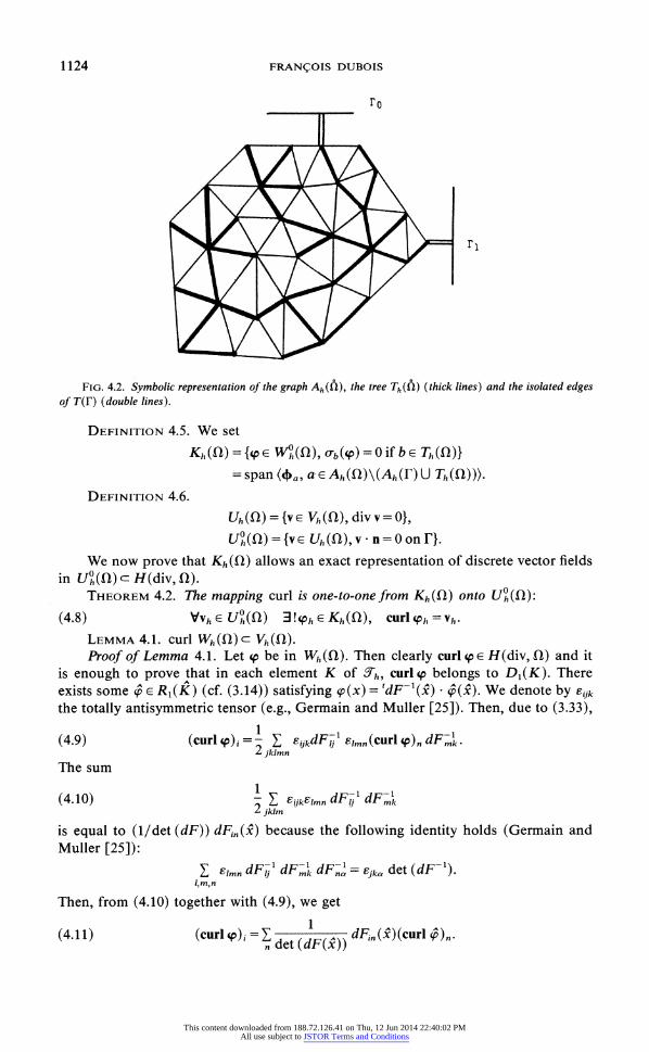
1124 FRAN4OIS DUBOIS
rO
FIG. 4.2. Symbolic representation of the graph Ah(f), the tree Th(Q) (thick lines) and the isolated edges of T(F) (double lines).
DEFINITION 4.5. We set
Kh(fQ) ={P E Woh(f), ab('P) = 0 if b E Th(Q)} -span (4a, a-e Ah(fQ)\(Ah(F) U Th(Q)))-
DEFINITION 4.6.
Uh (fQ) ={V E Vh(Q), div v = 0}, U? (f) -{ve Uh(Q), v - n= 0 on r}.
We now prove that Kh (Q) allows an exact representation of discrete vector fields in U? (f) c H(div, fl).
THEOREM 4.2. The mapping curl is one-to-one from Kh(Q) onto Uoh(Q):
(4.8) VVh E U (Q) 3!?ph E Kh(Q), curl iPh = Vh.
LEMMA 4.1. curl Wh(fi)c Vh(fQ).
Proof of Lemma 4.1. Let 'p be in Wh(f). Then clearly curl 'p E H(div, Q) and it is enough to prove that in each element K of 3h, curl p belongs to D1(K). There exists some E R1(K) (cf. (3.14)) satisfying qp(x) = tdF1 (x) x We denote by Eijk
the totally antisymmetric tensor (e.g., Germain and Muller [25]). Then, due to (3.33), 1
2 jklmn
The sum
(4.10) - E ijkElmn dF-1 dF-1 2 jklm
is equal to (1/det (dF)) dFin X) because the following identity holds (Germain and Muller [25]):
E ?lmn dFb1 dF-1 dFn-1 = 8jkaf det (dF-1). I,m,n
Then, from (4.10) together with (4.9), we get
(4.11) (curl 'p)= dF1(x)) in( ( (P)n
This content downloaded from 188.72.126.41 on Thu, 12 Jun 2014 22:40:02 PMAll use subject to JSTOR Terms and Conditions

DISCRETE VECTOR POTENTIAL IN THREE DIMENSIONS 1125
The vector curl p is constant in K, and thus it belongs to D1(K). Moreover, (4.11) shows that curl hp is in D1(K), due to (3.6). 0
LEMMA 4.2. We have the following characterization of U?h(Q):
(4.12) U (fl) = {v c H(div, Q), v - nlr = 0, 3i E (PO)3, (3.6) holds},
(4.13) dim Uh(fQ) = Nf-Ne + 1.
Proof of Lemma 4.2. * Let v be a vector-valued function of U? (Q). In the element K of 3h (3.6) allows
us to define i Dl. From (3.8) we easily deduce JKdivvdx=JRdivid?. Because div v =0 and div v is constant in K, v is constant on K, and the characterization (4.12) holds.
* Inversely, if v and v satisfy (3.6) we have the identity
div v(F(x)) = - div v(x) Vx^ E K, J = det dF(x),
which can be derived directly: by taking the divergence of (3.6), we get
(4.14) divv=EZ E dF&1 a (JdFij) +- div . j i,k Jk
The sum over i, k in (4.14) is null because we have the classical identity on determinants:
x (()=:J dFkil (
(dFik)- Xj i,k
k Xj
Then div v = 0 in K. Moreover, v - n is continuous along the faces of the mesh, and div v =0.
* The space U? (Q) is defined by Nf degrees of freedom and Ne relations due to (4.12). But the family of linear forms
Voh (QE) V XK, V) =Jdiv v dx E: f, K element of 3?h K
generates a linear space of dimension (Ne - 1) because we have the relation Z KE?h JK div v dx =0 for each ve Voh(Q). If we fix an element Ko, let us suppose that the following linear sum is null:
(4.15) Z aKXK = ?- K O KO
Fix K, $ K, 0 regular function verifying
supp 0 c KoU K1,
0>0 inK0, 0<0 inK1,
0 dx = 0.
We denote by (p a solution of the problem
Ap = 0 f, 8 =0o r, On
This content downloaded from 188.72.126.41 on Thu, 12 Jun 2014 22:40:02 PMAll use subject to JSTOR Terms and Conditions

1126 FRAN4OIS DUBOIS
and set v = rIhD(Vq). The vector v belongs to V?(fl) and according to Proposition 3.4 the integral JK div v dx is null for K different from Ko and K1, and is positive for K = K1. Then testing (4.15) on v, we get aK1 = 0, so (4.13) holds. 0
Proof of Theorem 4.2. * From Lemma 4. 1, curl is well defined Wh (fl) -* Uh (f). Moreover, if p belongs
to W?%(l), we have on the boundary of fl, curl p n- divy p x n = 0, then curl sp belongs to UO (IQ).
* The mapping curl Kh(Q1) -* U?h(Q7) is injective. Let sp be a vector lying in Kh(fQ), satisfying curl p = 0, and let a be an edge of Ah(fl)\(Ah(r) U Th(fl)). Following Proposition 4.2, there exists some discrete surface la from the triangulation -h with a boundary ya composed only of edges of {a} U Ah (r) U Th (Q). When we integrate curl sp on a,, we find J|, sp * ds = a,,(p), which is null because curl, = 0.
* The linear spaces Kh(fl) and Uh(fl) have the same dimension. On one hand, we clearly have dim Kh(fQ) = Na -,Nr ni - (N* -1) - (Nr+ 1), and on the other hand, thanks to Lemma 4.2, dim U?h(Q) = Nf* - Ne + 1. Moreover, Theorem 4.1 shows that N*-N* + Nf>Ne =-(Nr+ 1). Thus (4.8) holds. [
PROPOSITION 4.3. Suppose that -h satisfies Hypotheses 3.1, 3.2, and 4.1. Then for E: (W2(fl)n W1(f)), there exists (ph E Kh(l) such that
Ilcurl hp-curl Ph 110 Ql-_ Ch Ip11 W2(0)
for some C independent of h. Proof of Proposition 4.3. From Theorem 3.2, the H(curl) interpolate Il hRp in Wh (fQ)
satisfies
|| p 1r hRip ||Hcr )C Ch 11 ZP 11 W2(Q).
Moreover, fhlp E W?h(Q) since sp x n = 0 on afl. So curl (HRp) belongs to U?(fl) and verifies
IIcurl p -curl I-IhI110 R = Ch 11 P 11 W2(Ql).
Theorem 4.2 gives iPh in Kh(fl) satisfying
curl (Ph(X) = curl fh 9(X) VX E fl
and the proposition is established. 0
4.2. Mixed approximation and error estimate. We are now allowed to formulate a mixed discrete approximation of the continuous problem (4.1)-(4.3) in terms of a pair (Uh, 'h) in Uo(f) x Kh(Ql)-
PROPOSITION 4.4. Let f and g be two functions in (L2(Qk))3. The problem
Find (Uh, *h) E U(fQ) x Kh(f),
(4.16) Uh*Vh dx- curl 4h.' Vh dxj f Vh dx VVh E Uoh(f),
{uh curl 4Ph dx- g curl hph dx V4ph E Kh (fl)
admits a unique solution. Moreover, we have
(4.17) h|uh 0n + lIcurl 'h 110, lfIIo,n+211g110,0.
This content downloaded from 188.72.126.41 on Thu, 12 Jun 2014 22:40:02 PMAll use subject to JSTOR Terms and Conditions

DISCRETE VECTOR POTENTIAL IN THREE DIMENSIONS 1127
Proof of Proposition 4.4. * To prove that (4.16) admits a unique solution we need only consider the inf-sup
property [2], [11]:
(4.18) Ch>O Vh E Kh(Q) SUp - |Q curl (Ph * Vh dx (4.18) 3Ch>O V~~~PhheL4
sup -
Vh 11LP(n) ChliPh IIKh(n-). Vh C U?h (Q) |V lUh From Theorem 4.2, we can define a norm on Kh(fQ) by Ik PIIKh(n)= |curl ePIIO and we choose in U?(Q) the norm L2. Then, given (Ph in Kh, let us set vh = -curl (Ph. We get
in curl Ph * Vh dx |curl Ph vh dx dX sup -
- h11, IV 11, 11curl
(Ph 1 '
which demonstrates (4.18). * We now establish the stability property (4.17). Recall that we denote by (Uh, 'Ph)
the solution of (4.16). In the second equation of (4.16), take (Ph verifying curl (Ph = Uh-
We clearly deduce
(4.19) ||Uh 110, Q< 119 110,Q Now, choosing Vh = curl *h in the first equation, we get
l|curl 4h||O = {Uh curl 'h dx- f - curl 'h dx, Q Q (4.20) || curl 'h 11O O- Uh 11O,Q + 11 f 11O Q
Thus (4.17) is obtained by adding (4.19) and (4.20). 0 Remark 4.1. The mixed problem (4.16) always has one and only one solution for
each choice of the (small) parameter h. The stability property (4.17) gives good control of both Uh and curl 'h, which have a real physical meaning, but we have no control independent of h on the L2 norm of the vector potential 'h. This is natural: for each value of h, Definition 4.5 of Kh (fQ) holds in itself the choice of an arbitrary tree Th (fQ) and arbitrary edges of Th(F). Therefore it is hopeless to improve the L2 estimation with that kind of discrete gauge. Nevertheless, we recall that algebraically the linear system defined by (4.16) has a unique solution; the numerical tests we have achieved (see Appendices A below) show that for a given mesh the change of Th(fQ) has little impact on the difficulty of solving the linear system.
We now establish the main result of this part. Let X be a given vorticity function on fl:
to c(L 2(fl)) divto= 0, PNco= 0
Consider the velocity field u E (H1(fl))3 satisfying (4.1)-(4.3) (cf. Theorem 2.5). Con- sider also the L2 projection (Ah of X over U?(Q):
(4.21) COh E= Uoh(Q), ||"h 11 O,Q <II11IO 1 Qn
(4.22) f(Wb-0h).Vhdx=0 VVhE U%h(f1)
and the discrete problem
Uh E Uoh(f), 'h E Kh(Q),
(4.23) f UuW* Vh dx-i fcurl 'h' Vh dx = 0 vVh E (fi),
U h* curl (Ph dx =1 Xh * (Ph dx V(Ph E Kh(Q)-
This content downloaded from 188.72.126.41 on Thu, 12 Jun 2014 22:40:02 PMAll use subject to JSTOR Terms and Conditions
1128 FRANCOIS DUBOIS
We have the following theorem. THEOREM 4.3. Let o, C'h, u, and Uh be given as above. If Jh satisfies Hypotheses
3.1, 3.2, and 4.1, there exists some constant C (independent of h) such that
(4.24) IIU-Uh 11 1 ChIIto 11,. Remark 4.2. The practical computation of Vh is not easy (it requires the inversion
of the mass-matrix defined by the degrees of freedom in U?) and we note that ('h iS
not the H(div) interpolate of t. However, estimate (4.24) is of optimal order, as we have noted in the Introduction.
Proof of Theorem 4.3. We divide the proof in two parts. * First, we consider the continuous solution qh of
divqh=O fi,
(4.25) curl qh = h fl,
qh n=O F.
Let 'p E Wl(fQ). Its interpolate l D p belongs to U?(fl) due to Proposition 3.4; thus we have
(u - qh) - curl 'p dx= (O - Oh) * p dx
Xf (-O Xh) (. ( h - ) dx (thanks to (4.22))
? ~ -11R-( IIO,Q Ch IIpPII (cf. Theorem 3.1)
_ <-2ChjjlxiojjQIjjpjjj,Q (cf (4-21)),
(u-qh) - curl'p dx _ ChIItIIoj, curlhpIoj, Q according to Proposition 2.4. We now choose 'p as the vector potential of (u - qh)
thanks to Theorem 2.5; we get
(4.26) ilu -qh 11,n _ Ch 11colosQ.
* Second, the field qh introduced above in (4.25) admits a continuous potential Xh (according to Theorem 2.5) satisfying
qh Vdx - curl Xh * V dx = O Vv(L2(f))3,
fqh curl ( dx ={) h * . dx Vp E W1 (Q).
For now, let us fix (Uih, 'h) E Ux X Kh. Because Uo(fl) c (L (Q)), we have
(Uh -ih)Vh dx - curl (Ph -'Ph) dx
(4.27)
= (qh Uh) Vh dx curl (Xh -'Ph) * Vh dX VVh h Uh(Q)- Ql Q
This content downloaded from 188.72.126.41 on Thu, 12 Jun 2014 22:40:02 PMAll use subject to JSTOR Terms and Conditions
DISCRETE VECTOR POTENTIAL IN THREE DIMENSIONS 1129
Since Kh(fQ) is not included in Wl(fl), we must proceed otherwise with the second equation. We multiply the second line of (4.25) by SPh E Kh(fQ) and integrate by parts (cf. (1.21)), and the boundary term vanishes because (Ph X n = 0. Thus we have
(4.28) f qh curl (Ph dx =i h * Ph dx.
We subtract (4.28) from the second equation of (4.23), and obtain
(4.29) f(Uh -Uh) -curl Ph dX (qh-uh)curl(Phdx VPhcEKh(Q).
Then the pair (Uh - Uh, Ih - 'h) is the solution (due to (4.27) and (4.29)) of a mixed discrete problem (4.16). Proposition 4.4 gives stability:
||Uh- h|llo Q _C( liqh-UhllO Q +llcurl (Xh vh )110,Q)- Then, using the triangle inequality, we get
lUh -qhIIO,n_ C inf {Iqh -UhII0,n + Ilcurl (Xh -Ph)IO,O} U h fEU?h, f,hE Kh
Now, for Uh (respectively, 'h) take the interpolate in U (fQ) (respectively, Kh(fQ)) defined according to Theorem 3.1 (respectively, Proposition 4.3) of qh (respectively, Xh)- We deduce
h|Uh-qh jIIo, : Ch(jjqh II1,Q IIXh 11 W2(Q)
_ Ch 1II)h IIo,n (cf. Theorem 2.5),
(4.30) 11uh-qhjj|,n-' Chjj(loj,n (cf (4.21)).
The conclusion of the theorem follows from (4.26) and (4.30). 0
5. The Dirichlet boundary condition. In this last section we focus on the approxima- tion of a harmonic vector field u with given mass inflow and outflow on the boundaries
(5.1) div u = fl,
(5.2) curlu=0 fQ,
(5.3) u*n=g F.
We suppose that
(5.4) fgdy= 0 Vi=0,1, ,Nr
to be sure that u admits a representation in terms of a vector potential ' (cf. Proposition 2.5): u = curl '. Moreover, a boundary equation is satisfied by the tangential component r1* on afl:
(5.5) curlrIfr1=g onF.
We first study an approximation of (5.5): we recall the results of Bendali [3], [5] and Nedelec [36] for constructing vectorial finite elements on the boundary, and we propose a discrete gauge condition to ensure the uniqueness of the tangential component in a discrete version of (5.5). Second, we use a discrete extension to replace the one in the homogeneous case studied in ? 4.
This content downloaded from 188.72.126.41 on Thu, 12 Jun 2014 22:40:02 PMAll use subject to JSTOR Terms and Conditions

1130 FRANCOIS DUBOIS
The boundary F admits (Nr+ 1) simply connected components Fi, and (5.5) is thus decoupled in (Nr + 1) different boundary equations. Therefore in ?? 5.1 and 5.2 we look at a connected manifold Fi, and in ? 5.3 we study the boundary F of fQ.
5.1. Finite elements on the boundary. In ? 3 we have developed curved finite elements to ensure that the approached domain h is exactly fl. Moreover, the boundary afl is exactly covered by curved faces of the triangulation 3h. We will denote by 3Jh(F) the mesh defined on F by Jh (i.e., the points Ph(F), the edges Ah(F), and the curvilinear triangles that are the faces of F). We can suppose that each triangle k of Jh(F) is the range of k ={(X1, X^2, O) 3, X2 X X^-+2_ 1} by the mapping F defined in (3.1). Moreover, as k is a face of K (Definition 3.1), the triangle k is a face of some curved tetrahedron K of Jh, and we denote by Fk the restriction of F to k. The straight terahedron K defined by the vertices of K, and parameterized by K 3 x(Bx~ + b) E K, defines a plane triangle k whose union recovers an approximated surface Fh of F. In Fig. 5.1 we show that k is parameterized by k due to the normal projection Pr on the surface k 3 XX = Pr(:) c k as first proposed by Nedelec [34].
n(x)
FIG. 5.1. Curvilinear triangle on the boundary.
Moreover, let (ei)i=1,2,3 be the canonical basis of 3. The total Gaussian curvature G(x) and the normal n(x) of F at the point x = F(x) of k admit the expressions
G(x) = ldF( )x e x dF(x^) x 2I2,
n(x) = , (dF(x) e x dF(x) 2
n(x) = N x (dFk(x) el x dFk(x) x 2)
This content downloaded from 188.72.126.41 on Thu, 12 Jun 2014 22:40:02 PMAll use subject to JSTOR Terms and Conditions

DISCRETE VECTOR POTENTIAL IN THREE DIMENSIONS 1131
DEFINITION 5.1 (Nedelec [36]).
R -7: k - D 3a, 8,yER ?, Al() = ae + , 72(A) = _ A3Yll.
DEFINITION 5.2. Local spaces for the approximation of tangent vectors on F:
R'(k)= k 3 R'x/Ck k(F(C))= 1 dF(x) 4 The global finite-element spaces for the interpolation of densities (which belong
to M(F)) and currents (lying in TH1/2(r)) are now given. DEFINITION 5.3.
Mh(F) = wL2(), Vk E h (F), 3 WAE R, VxE k, w(F(x)) = , j w dy =O
For two triangles k, 1 of 3"h(F) intersecting each other in an edge a, we denote by Tk
and T, the two tangent vectors that are compatible with the orientation defined on k and 1 by the external normal to F (Fig. 5.2). We set
Xh(F) = F-- R3, Vk EJ h(F), F k e Rl(k),
(5.6) Va=knl edge of 5h (F), ia ( Tk +q *T1) ds=0I.
a~~~~~~
n k
FiG. 5.2. Adjacent triangles on the boundary.
The degrees of freedom in Mh(F) and Xh(F) are, respectively, OTk(W)=
Jk W(x) dy(x), k E 3Zh(F) and Xa = {UaQra l) = fa 1- ds, a edge of $?Th(F)}. We now define interpolation operators in Mh(F) and Xh(F).
THEOREM 5.1 (Nedelec [34]). There exists an operator P': L2(F) n M(F) -> Mh(F) defined by Jk Phsw dy = Jk w dy, for all k Ec h (F), and if $Th is regular (Hypotheses 3.1, 3.2) we have
(5.7) 1w - Psw|L12,v ChI |w11112,, wE H1/2(r)
for some constant C. THEOREM 5.2 (Bendali [5]). Let s be real, s > 2. There exists an interpolation operator
pc THs(F) - Xh (F) defined by Ja P 11 * ds = Ia 1 - ds, a edge on Sh; we have
This content downloaded from 188.72.126.41 on Thu, 12 Jun 2014 22:40:02 PMAll use subject to JSTOR Terms and Conditions

1132 FRANCOIS DUBOIS
PROPOSITION 5.1. We have the following relations between Xh(F), Mh(F) and the curl operator on F:
(5-8) curl Xh(F) c Mh(F),
(5.9) Phs(curlr V)= curlrq(P c) E THS(F), s>1.
Proof of Proposition 5.1. * The inclusion curlr Xh c L2(r) is a direct consequence of the continuity of the
tangential component -V Ta of the functions q c Xh (F) on the edges a of Sh (F) according to (5.6). Moreover, the integral of curlr q on F is always null and curlr Xh Mh(F). In each triangle k of Wh(F) we have the general identity
curlr{j dF 1=j, (curla2 77)
Thus, if q belongs to R'(k), then 7 lies in R' and curl?R2 ' is a constant function, which implies (5.8).
* The proof of (5.9) is standard-integrate Ps(curlr ,i) on k:
Ps(curlr ,) dy = curlr a dy = divr (l x n) dy k k k
1K x xn- v ds (cf. Fig. 5.3) 9K
= ds=J pqP -ds= curlr (Psc) dy. aK aK k
Thus the two functions of (5.9) have the same degrees of freedom in Mh(F). Therefore they are equal. O
5.2. Approximation of the boundary problem. We first define a discrete subspace of Xh(F) in which the curlr operator is one-to-one onto Mh(F).
DEFINITION 5.4. We define 9)a as the natural basis of Xh(F), parameterized by the graph Ah (r) of the edges of ih (r): Oa (Nb) = 8a,b for a, b edges of ih (F).
DEFINITION 5.5. Let us consider a given tree Th(F) in the graph Ah(F). We set
Yh (F) = span (,Qa, a c Ah ()\ Th (F))-
THEOREM 5.3. The operator curlr is one-to-one from Yh(F) onto Mh(F):
VWh c Mh(F) 3!h C Yh(F), curlrFh = Wh
n
FIG. 5.3
FIG. 5.3
This content downloaded from 188.72.126.41 on Thu, 12 Jun 2014 22:40:02 PMAll use subject to JSTOR Terms and Conditions

DISCRETE VECTOR POTENTIAL IN THREE DIMENSIONS 1133
Proof of Theorem 5.3. * First, the spaces Yh(F) and Mh(F) have dimensions na - (n, -1) and nf -1,
respectively; those numbers are equal, according to Theorem 4.1, due to the Euler characteristic.
* Second, curlr is injective on Yh(F). The proof given for Theorem 4.2 is the same. Let a be an edge of Ah(F)\Th(r); the cycle ya generated by a and Th(F) is the boundary of some discrete surface la over which we integrate the null scalar curly iq(q C Yh(F)). We find JI, curlr q dy = aa(-1) = 0. This statement is true for each edge a of Ah(F), and therefore q = 0. O
Now let g be a given scalar function of H112(r) n M(F) and let t be the (unique) solution lying in W112(r) of the continuous problem (cf. Proposition 2.7):
(5.10) curlr t= g, divr, = 0
whose mixed variational formulation is (see (2.24))
e w1'2(r), 0 a L2(r) n M(r),
(5.11) Ig - - dy- i0 curlr,
- dy = V-q
W1'(r)
fcurlr gw d= gw dy Vw c L2(r) n M(r).
We denote also by gh the interpolate of g in Mh(F). We have, according to Theorem 5.1,
(5.12) 1I - gh ||-1/2,1 -Ch 11 g 11| 2, DEFINITION 5.6. We will denote in the following by th the unique vector valued
function of Yh (F) such that
(5.13) curlr th = gh-
Due to (5.10) and (5.12) we have
(5.14) I| curlr, - curlr ih II -1/2,v r Ch || g 1| 1/2,F-
Remark 5.1. The discrete gauge on the boundary gives a solution th of (5.13) that is very easy to compute; there indeed exists an enumeration of the edges (related to the tree Th(F)) such that (5.13) is reduced to a triangular system. The idea of decoupling the discrete gauge in the domain (? 4) and on the boundary was first proposed by Roux [41] in a particular case.
5.3. Extension of the boundary problem. We now solve the part of the original problem (5.1)-(5.4) corresponding to zero prescribed vorticity in fQ and a given nonzero mass flow g on the boundary F of fl. The spaces Xh(Fi) and Yh(Fi) introduced previously can be viewed as subspaces of Wh(fl) (cf. Definition 3.4).
DEFINITION 5.7. Let 4,,, a E Ah(fQ), be the basis of Wh(fQ) introduced in Definition 4.3, and let Th(Fi) be given trees on the subgraphs Ah(Fi). We set
Xh(fl)=span(4a, aeAh(Fi), i=0, * *, NY),
Yh(fl) = span (4)a, a E Ah(ri)\Th(ri), i = O, . -, Nr).
PROPOSITION 5.2. If p belongs to Xh(fQ) (respectively, Yh(fQ)), its tangential com- ponent rlp belongs to xh(ri) (respectively, Yh(Fi)) for some i.
This content downloaded from 188.72.126.41 on Thu, 12 Jun 2014 22:40:02 PMAll use subject to JSTOR Terms and Conditions

1134 FRANCOIS DUBOIS
Proof of Proposition 5.2. This is a consequence of the H(curl, fQ) unisolvence of (K, Xa, R1(K)) proved in Proposition 3.2: the tangential components of sp on the face k are only a function of the degrees of freedom 0a (ip) for the edges a of ak. Moreover, we see easily that the spaces R'(k) are exactly the sets of tangential components on k of the functions of R1(K). The statement is thus established. 0
PROPOSITION 5.3. Suppose that Jh satisfies Hypotheses 3.1, 3.2, and 4.1. Let us now give g in H112(r) n M(r), verifying lJy g dy = 0 for i = 0, 1, - * *, Ny. We consider the solution t of (5.11), the interpolate gh of g in Mh(F) e ;rrO Mh(Fi). There exists th e Yh (f) satisfying
(5.15) curlrfflh= gh,
(5.16) l|curlrv - curlr rlth II -1/2, r_ Ch II g 1| 1/2,F
for some constant C. Proof. The proof is a direct consequence of (5.14) and Proposition 5.2. 0 PROPOSITION 5.4. Let g, gh, and h be defined as above, and let u be the solution
of (5.1)-(5.3). The vector rlDu-curl h belongs to U?(fl), and we set
(5.17) 1uh Ih - curlth-
Proof of Proposition 5.4. The scalar function div rlDU is equal to zero according to Proposition 3.4. Moreover, due to Lemma 4.1, curl th belongs to Uh(fl). We deduce that uh belongs also to Uh(fl). Then we just have to prove that the normal component (h - curl h) * n is null on F, i.e., that its integral on each face is null, according to Lemma 4.2. But we have
h indy= u-ndy (cf. (3.10)) k k
=f gdy (cf.(5.3)) k
={ ghdy (cf.(5.7))
= curlr rlth dy (cf. (5.15))
=|curl h -n dy (cf.Lemma2.1). D
THEOREM 5.4. Let g, u, gh, th, Uh be defined as in Proposition 5.4. Consider Uh,
represented as Uh = curl th + Vh, with Vh a solution of the discrete mixed problem
Vh E Uoh(fi), * h E- Kh (fl),
(5.18) } vh whdx curl*h'hWhdx=0 VWhE Uh,
fVhh curl Ph dx=-f curl h -curl hPhdx Veph c Kh-
Then, if 3Th satisfies Hypotheses 3.1, 3.2, and 4.1, we have
This content downloaded from 188.72.126.41 on Thu, 12 Jun 2014 22:40:02 PMAll use subject to JSTOR Terms and Conditions

DISCRETE VECTOR POTENTIAL IN THREE DIMENSIONS 1135
Proof of Theorem 5.4. * We first consider the solution v of the continuous problem
divv=O Q
curl v =-curl h fQ,
v * n=0 r,
or
V E- (L 2(fl))35 t E=w (fl()
(5.19) fv -wdx-f curl*-wdx=0 VwC(L2(fl))3,
fv curl hp dx =- curl h* curl hp dx Vp E Kh (f)-
The field u - (v + curl th) is harmonic (its divergence and curl are null) and its normal component on F is exactly (g - gh). Due to Proposition 2.9 and (5.12) we have
(5.20) 1IIu-(v+curl th)II0,|O Q Ch 11 g1112,v * We need only establish a similar inequality for the vector Uh - v - curl gh = Vh - V.
Let (Ph be in Kh(fQ). Then curl (Ph E (L2(fQ))3 and Theorem 2.4(i) gives
(5.21) curl (Ph= Vp + curl p
with p E H1 n Lo P EC W1. Because rAh = 0 if (Ph E Kh(fQ) we have divr (Ph xn = 0 and finally p = 0. We insert the function sp defined in (5.21) as a test function in the second equation of (5.19). We get in v curl Ph dx = -|Q curl g, - curl (Ph dx, for all (Ph E Kh(f),
and by subtracting from (5.18) we deduce, due to Theorem 4.2, the equality
(5.22) I(v- Vh) * Wh dx = 0 VWh E Uh(fQ)-
However, we have
(5.23) v-wh= (v+ rot 4h-u) + (u (roth + Wh))-
We choose Wh = uh of (5.17). According to (5.22) and (5.23)
IIV-Vh II O,nQ IIV- Uh II O,Q
I_ ||-(v+ curl 0h)||0,1 I|U - rh U|loQ
_Ch 11 g 11 /2,]F Ch II UII 1,Q; then
(5.24) IIV-Vh || I,O _ Ch 11 g 11 1/2,r
due to Theorem 2.4(i). Inequalities (5.20) and (5.24) prove the theorem. D
6. Conclusion. In this paper, we have studied the discretization of a solenoidal vector field through the curl of a vector potential. We have recalled that two gauge conditions must be prescribed for this potential, which are both written with divergence operators. We have seen in ?? 4 and 5 that these conditions have a discrete analogy in terms of trees in the graph defined by the edges of the mesh. The error estimates obtained only concern the solenoidal field because the arbitrary choice induced by the discrete gauges does not ensure any a priori simple L2 stability for the potential.
This content downloaded from 188.72.126.41 on Thu, 12 Jun 2014 22:40:02 PMAll use subject to JSTOR Terms and Conditions
1136 FRANfOIS DUBOIS
A direct application of this work is the numerical study of compressible flow and incompressible Navier-Stokes equations developed at Ecole Polytechnique at Palaiseau (Dubois and Dupuy [18], [19], Roux [41]). This study of the numerical error order could be followed in different fields: for example, to treat approximations of arbitrary order using the H(curl) conforming elements proposed by Nedelec [37] and more recently by Brezzi, Douglas, and Marini [12] and Nedelec [39]. On the other hand, the hypothesis of smooth boundary could be avoided and we could study more realistic physical problems of fluid dynamics such as the Stokes problem in DR3 in (I, c) formulation (Girault and Raviart [26], Nedelec [38]). Finally, the discrete gauge could be generalized to non-simply connected domains of R3.
Appendix A. A numerical experiment. The matter presented above explains rigorously how to approximate a divergence-free vector field in DR3 with a vector potential conforming in H(curl) when the domain admits a smooth (eventually noncon- nected) boundary. In practice, most of the computational domains have a polyhedral boundary and the analysis is not applicable. Nevertheless, the numerical procedure developed in ?? 4 and 5 can be applied without any modification when afl is polyhedral. In this appendix we show that the numerical algorithms described previously can be implemented without any trouble in the case of a very simple problem. More precisely, the discrete spaces Kh(fQ) (respectively, Yh(ft)) introduced in Definition 4.5 (respec- tively, Definition 5.7) can be constructed without the help of curved finite elements. However, the practical construction of the trees Th (fQ) and Th (r) gives the user a great number of degrees of freedom in the choice of the spaces Kh(fQ) and Yh(fQ).
In the following we present the practical solution of a very simple problem posed on Ql = (]0, 1[)3. We have used prismatic finite elements instead of tetrahedrons, and we describe quickly the associated discrete function spaces. The choice of the tree Th(fQ) on the boundary is that of Roux [41]. The three-dimensional stream function is computed by solving a positive definite, symmetric system with a conjugate gradient method. We also present two different choices of the internal tree Th (ft) and their relative influence on the practical solution of the linear system.
A.1. The test case. The domain fl is the cube (]0, 1[)3. The face (]0, 1[)2 x (0) corresponds to the inflow, and the opposite face to the outflow. We solve the problem
(Al) divu=0 fQ,
(A2) curl u = 0 f,
(A4) u n=-1, ri=(]o, 1[)2x(0),
(A4) u *n = + 1, ro = (io, 1[)2 x (1),
(A5) u n=0, rtF=av\(riUro). The exact solution of the system (A1)-(A5) can be obtained in a straightforward manner, and we have
u--(0,0,1)--e3.
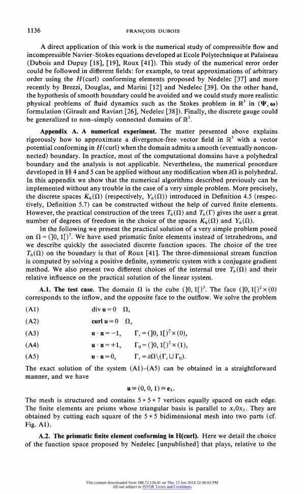
The mesh is structured and contains 5 * 5 * 7 vertices equally spaced on each edge. The finite elements are prisms whose triangular basis is parallel to xI0x2. They are obtained by cutting each square of the 5 * 5 bidimensional mesh into two parts (cf. Fig. Al).
A.2. The prismatic finite element conforming in H(curl). Here we detail the choice of the function space proposed by Nedelec [unpublished] that plays, relative to the
This content downloaded from 188.72.126.41 on Thu, 12 Jun 2014 22:40:02 PMAll use subject to JSTOR Terms and Conditions

DISCRETE VECTOR POTENTIAL IN THREE DIMENSIONS 1137
x3
x
FIG. Al. View of the surface tree Th(F) on the boundary of the cube ]O, 1[3. The boundary edges, associated with the degrees offreedom that are a priori not null, are represented by a double line.
prism, the same role as the space R1 for tetrahedrons (cf. Definition 3.4). We restrict ourselves to the "unity prism" K:
K ={(x1,x2,x3)EH3 o-xi -x1+x2?-1}.
Then the procedure explained in (3.7) (Definition 3.5) can be applied without modification for any given prism. The interpolate vector potential admits the following form:
a + cx3 -(e +fx3)x2 O p(x) = b + dx3 + (e +fx3)XI + 0 forX= (X1, X2, X3)
A
K O a <+J8XI + X2
and depends on the nine real parameters a, b, c, d, e, f, a, /3, y. The corresponding degrees of freedom are the circulations
a('p) = Jp ds, a an edge of the mesh a
as previously, and it is possible to show that the corresponding finite element associated with that choice of geometry, degrees of freedom, and function space is unisolvent and conforming in H(curl).
A.3. Surface gauge. From the particularity of boundary conditions (A3)-(A5), Roux [41] developed a procedure to construct a particular tree Th(F), and consequently the space Yh(fl) of the functions th such that
(A6) curl,,h n=u * n onEal.
This choice ensures that the homogeneous boundary condition (A5) is always satisfied. The result is presented in Fig. Al: the tree Th (r) is composed by two subtrees on each
This content downloaded from 188.72.126.41 on Thu, 12 Jun 2014 22:40:02 PMAll use subject to JSTOR Terms and Conditions

1138 FRANMOIS DUBOIS
face r, and ro. The edges a such that oa((P) is not null a priori are represented by a double line. For more details, we refer to [41] and [19]. Computing th satisfying (A6) (or (5.15)) is easy after finding an optimal enumeration of the edges that transforms (A6) into a triangular system. Due to the (relatively) low cost of this step of the algorithm (compared with the next step; the orders of systems (A6) and (A7) are, respectively, 69 and 249 for our test problem), this procedure has not been compared with a direct Gaussian elimination.
A.4. Solution of the internal problem. Here we focus on the computation of the stream function th +?h of the discrete velocity field, with th given in the preceding section and *h E Kh(fQ) determined by solving problem (5.18). We remark that this mixed problem can be rewritten in terms of the only vector potential lh according to Theorem 4.2 (but this is not the case for a general system such as (4.16)). Then problem (5.18) is equivalent to
Wh E Kh (Q),
(A7) {curlPh - curl qh dx=-J curlth -curl shpdx Vph EKh(fQ)-
We recover (as in [18]) a classical conforming variational formulation. The matrix associated with (A7) is symmetric positive definite. We have used a conjugate gradient method (see, e.g., Lascaux and Theodor [47]) for solving the problem (A7). We have tested two preconditioners: the incomplete Cholesky factorization and the SSOR factorization of Evans (see, e.g., [47]). The first has given negative roots during the algorithm with the choice of the internal tree Th(fQ) pictured on the Fig. A2. This fact proves that the matrix defined by (A7) is a priori not an M-matrix, according to Meijerink and Van Der Vorst [48]. A performing choice for the preconditioner is finally the SSOR factorization that we retain in our present computation as well as for more
FIG. A2. First choice for the internal tree Th(fl) inside the domain.
This content downloaded from 188.72.126.41 on Thu, 12 Jun 2014 22:40:02 PMAll use subject to JSTOR Terms and Conditions

DISCRETE VECTOR POTENTIAL IN THREE DIMENSIONS 1139
complicated problems [18]. The discrete velocity field
Uh = curl ((h + ?h)
is in fact the exact solution e3 since the latter belongs to the affine space curl ((h + Kh (M)) as we verified numerically. We emphasize that the discrete vector potential (h +? h
has no elementary analogue and, in particular, has no simple relation to the following family of the polynomial vector potentials 'p:
', = 2 e3 x x + grad 0, + polynomial.
We end this appendix with a comparison between the uses of the two internal trees of Figs. A2 and A3. The first tree is composed of a majority of horizontal edges, whereas the second contains essentially vertical edges. The first (Fig. A2) leads to a better performance for the conjugate gradient algorithm (40 iterations with the SSOR preconditioner to reach an error of 10-4 relative to the operator 12 norm, and 74 iterations with the second tree). Curiously, the condition numbers Amax/Amin of the two matrices are, respectively, 14,150 (first tree) and 6,811 (second tree). This last numerical result shows the great complexity of the distribution of the eigenvalues in the spectrum, according to Jennings [49]. We have also tested other possibilities for the tree Th(fQ) (see [19]), but no simple correlation appears between the geometric location of the edges in Th (fQ) and the performance of the conjugate gradient algorithm (see also Remark 4.1). Nevertheless, in all the practical situations that we have been confronted with [18], [19], [41], the linear system (A7) has been solved efficiently with the SSOR preconditioner.
Acknowledgments. I thank F. X. Roux and J. M. Dupuy for their intense collabor- ation during the implementation of the Nedelec H(curl) finite element, G. Laumon
x3
FIG. A3. Second choicefor the internal tree Th(fl) inside the domain.
This content downloaded from 188.72.126.41 on Thu, 12 Jun 2014 22:40:02 PMAll use subject to JSTOR Terms and Conditions

1140 FRANMOIS DUBOIS
for a helpful discussion about algebraic topology, and the first referee for useful comments and suggestions.
REFERENCES
[1] R. A. ADAMS, Sobolev Spaces, Academic Press, New York, 1975. [2] I. BABUSKA, Error-bounds for thefinite element method, Numer. Math., 16 (1971), pp. 322-333. [3] A. BENDALI, Approximation par elmentsfinis de surface deproblemes de diffraction des ondes electromag-
netiques, These d'etat, University of Paris, Paris, 1984. [4] , Numerical analysis of the exterior boundary value problem for the time harmonic Maxwell equations
by a boundary finite element method. Part 1: the continuous problem, Math. Comp., 43 (1984), pp. 29-46.
[5] , Numerical analysis of the exterior boundary value problem for the time harmonic Maxwell equations by a boundaryfinite element method. Part 2: the discrete problem, Math. Comp., 43, (1984), pp. 47-68.
[6] A. BENDALI, J. M. DOMINGUEZ, AND S. GALLIC, A variational approach for the vector potential formulation of the Stokes and Navier-Stokes problems in three dimensional domains, J. Math. Anal. Appl., 107 (1985), pp. 537-560.
[7] A. BENDALI AND S. GALLIC, Formulation du systeme de Stokes en potentiel vecteur, Internal Report 79, Centre de Mathematiques Appliquees, Ecole Polytechnique, Palaiseau, France, 1982.
[8] C. BERGE, Graphes et hypergraphes, Dunod, Paris, 1970. (English translation, North-Holland, Amster- dam, New York, 1973.)
[9] C. BERNARDI, Methodes d'e'ements finis mixtes pour les equations de Navier-Stokes, These de 3eme cycle, University of Paris, Paris, 1979.
[10] J. H. BRAMBLE AND S. R. HILBERT, Bounds for a class of linear functionals with applications to Hermite interpolation, Numer. Math., 16 (1971), pp. 362-369.
[11] F. BREZZI, On the existence, uniqueness and approximation of saddle point problems arising from Lagrangian multipliers, RAIRO, R2 (1974), pp. 129-151.
[12] F. BREZZI, J. DOUGLAS, AND L. D. MARINI, Two families of mixed finite elements for second order elliptic problems, Numer. Math., 47 (1985), pp. 217-235.
[13] Y. CHOQUET-BRUHAT, G&omtrie differentielle et systemes exterieurs, Dunod, Paris, 1968. [14] P. G. CIARLET, The Finite Element Method for Elliptic Problems, North-Holland, Amsterdam, New
York, 1978. [15] R. COURANT AND K. 0. FRIEDRICHS, Supersonic Flow and Shock Waves, Interscience, New York, 1948. [16] G. DE RHAM, Varietes differentiables, Hermann, Paris, 1955. [17] J. M. DOMINGUEZ, These de 3eme cycle, University of Paris, Paris, France, 1982. [18] F. DUBOIS AND J. M. Dupuy, A three-dimensional vector potential formulation for solving transonic
flows with mixed finite elements, in Proc. 6th International Symposium: Finite Element Methods in Flow Problems, Antibes, France, 1986.
[19] F. DUBOIS, Quelques problemes lies au calcul d'ecoulements defluides parfaits dans les tuyeres, Doctoral thesis, University of Paris, Paris, France, 1988.
[20] G. DUVAUT AND J. L. LIONs, Les inequations en mfecanique et en physique, Dunod, Paris, 1972. [21] F. EL DABAGHI AND 0. PIRONNEAU, Stream vectors in three-dimensional aerodynamics, Numer. Math.,
48 (1986), pp. 561-589. [22] C. FOIAS AND R. TEMAM, Remarques sur les equations de Navier-Stokes stationnaires et lesphenomenes
successifs de bifurcation, Ann. Scuola Norm. Sup. Pisa Cl. Sci. (4), 5 (1978), pp. 29-63. [23] K. 0. FRIEDRICHS, Differentialforms on Riemannian manifolds, Comm. Pure Appl. Math., 8 (1955),
pp. 551-590. [24] V. GEORGESCU, Some boundary value problems for differentialforms on compact Riemannian manifolds,
Ann. Math Pura Appl. (4), 122 (1979), pp. 159-198. [25] P. GERMAIN AND P. MULLER, Introduction a la mecanique des milieux continus, Masson, Paris, 1980. [26] V. GIRAULT AND P. A. RAVIART, Finite Element Methods for Navier-Stokes Equations. Theory and
Applications, Springer-Verlag, Berlin, New York, 1986. [27] J. GLIMM, personal communication, 1986. [28] K. GUSTAFSON AND R. HARTMAN, Divergence-free bases forfinite element schemes in hydrodynamics,
SIAM J. Numer. Anal., 20 (1983), pp. 697-721. [29] F. HECHT, Construction d'une base de fonctions P1 non conforme a divergence nulle dans R3, RAIRO
Anal. Numer., 15 (1980), pp. 315-341. [30] J. D. JACKSON, Classical Electrodynamics, John Wiley, New York, 1962.
This content downloaded from 188.72.126.41 on Thu, 12 Jun 2014 22:40:02 PMAll use subject to JSTOR Terms and Conditions

DISCRETE VECTOR POTENTIAL IN THREE DIMENSIONS 1141
[31] M. LENOIR, Optimal isoparametric finite elements and error estimates for domains involving curved boundaries, SIAM J. Numer. Anal., 23 (1986), pp. 562-580.
[32] J. L. LIONS AND E. MAGENES, Problemes aux limites non homogenes et applications, Vol. 1, Dunod, Paris, 1968.
[33] W. S. MASSEY, Algebraic Topology: An Introduction, Harcourt, Brace, and World, New York, 1967. [34] J. C. NEDELEC, Curvedfinite element methodsfor the solution of singular integral equations on surfaces
in 3, Comp. Meth. Appl. Mech. Engrg., 8 (1976), pp. 61-80. [35] , Approximation des equations integrales en mecanique et en physique, Cours CEA-EDF-INRIA,
Paris, 1977. [36] , Computation of eddy currents on a surface in 3 by finite element methods, SIAM J. Numer.
Anal., 15 (1978), pp. 580-594. [37] , Mixedfinite elements in 3, Numer. Math., 35 (1980), pp. 315-341. [38] ' Elements finis mixtes incompressibles pour l'equation de Stokes dans 3, Numer. Math., 39
(1982), pp. 97-112. [39] , A newfamily of mixedfinite elements in R3, Numer. Math., 50 (1986), pp. 57-81. [40] P. A. RAVIART AND J. M. THOMAS, A mixed finite element method for second order elliptic problems,
Lecture Notes in Math. 606, Springer-Verlag, Berlin, New York, 1977. [41] F. X. Roux, Lecture, University of Paris, Paris, March 1984; Doctoral thesis, University of Paris,
Paris, to appear. [42] R. ScoTT, Interpolated boundary conditions in the finite element method, SIAM J. Numer. Anal., 12
(1975), pp. 404-427. [43] R. TEMAM, Navier-Stokes Equations, North-Holland, Amsterdam, New York, 1977. [44] F. TREVES, Introduction to Pseudodifferential and Fourier Integral Operators, Vol. 2, Plenum Press, New
York, 1980. [45] M. ZLAMAL, Curved elements in the finite element method I, SIAM J. Numer. Anal., 10 (1973), pp.
229-240. [46] , Curved elements in the finite element method II, SIAM J. Numer. Anal., (1974), pp. 347-362. [47] P. LASCAUX AND R. THEODOR, Analyse numerique matricielle appliquee a l'art de l'inge'nieur, Masson,
Paris, 1986. [48] J. A. MEIJERINK AND H. A. VAN DER VORST, An iterative solution methodfor linear systems of which
the coefficient matrix is a symmetric M-matrix, Math. Comp., 31 (1977), pp. 148-162. [49] A. JENNINGS, Influence of the eigenvalue spectrum on the convergence rate of the conjugate gradient
method, J. Inst. Math. Appl., 20 (1977), pp. 61-72.
This content downloaded from 188.72.126.41 on Thu, 12 Jun 2014 22:40:02 PMAll use subject to JSTOR Terms and Conditions