Embed Size (px)
Citation preview
VECTOR CALCULUSVECTOR CALCULUS
17
2
17.9The Divergence Theorem
In this section, we will learn about:
The Divergence Theorem for simple solid regions,
and its applications in electric fields and fluid flow.
VECTOR CALCULUS
3
INTRODUCTION
In Section 17.5, we rewrote Green’s Theorem
in a vector version as:
where C is the positively oriented
boundary curve of the plane region D.
div ( , )C
D
ds x y dA F n F
4
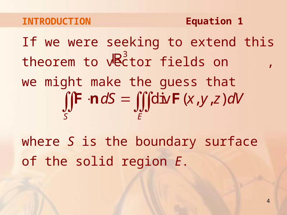
INTRODUCTION
If we were seeking to extend this theorem to
vector fields on , we might make the guess
that
where S is the boundary surface
of the solid region E.
3
div ( , , )S E
dS x y z dV F n F
Equation 1
5
DIVERGENCE THEOREM
It turns out that Equation 1 is true,
under appropriate hypotheses, and
is called the Divergence Theorem.
6
DIVERGENCE THEOREM
Notice its similarity to Green’s Theorem
and Stokes’ Theorem in that:
It relates the integral of a derivative of a function (div F in this case) over a region to the integral of the original function F over the boundary of the region.
7
DIVERGENCE THEOREM
At this stage, you may wish to review
the various types of regions over which
we were able to evaluate triple integrals
in Section 16.6
8
SIMPLE SOLID REGION
We state and prove the Divergence Theorem
for regions E that are simultaneously of types
1, 2, and 3.
We call such regions simple solid regions.
For instance, regions bounded by ellipsoids or rectangular boxes are simple solid regions.
9
SIMPLE SOLID REGIONS
The boundary of E is a closed surface.
We use the convention, introduced in
Section 17.7, that the positive orientation
is outward.
That is, the unit normal vector n is directed outward from E.
10
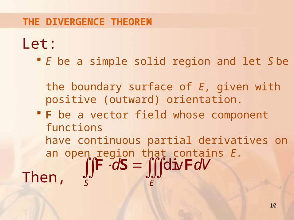
THE DIVERGENCE THEOREM
Let: E be a simple solid region and let S be
the boundary surface of E, given with positive (outward) orientation.
F be a vector field whose component functions have continuous partial derivatives on an open region that contains E.
Then, div
S E
d dV F S F
11
THE DIVERGENCE THEOREM
Thus, the Divergence Theorem states
that:
Under the given conditions, the flux of F across the boundary surface of E is equal to the triple integral of the divergence of F over E.
12
GAUSS’S THEOREM
The Divergence Theorem is sometimes
called Gauss’s Theorem after the great
German mathematician Karl Friedrich Gauss
(1777–1855).
He discovered this theorem during his investigation of electrostatics.
13
OSTROGRADSKY’S THEOREM
In Eastern Europe, it is known as
Ostrogradsky’s Theorem after the Russian
mathematician Mikhail Ostrogradsky
(1801–1862).
He published this result in 1826.
14
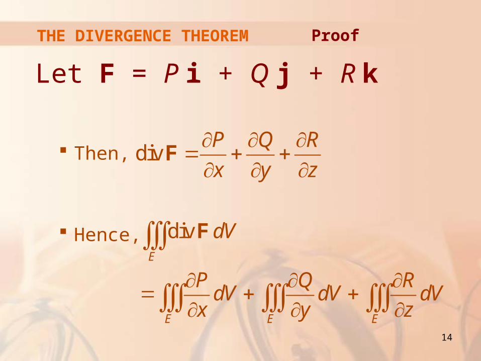
THE DIVERGENCE THEOREM
Let F = P i + Q j + R k
Then,
Hence,
divP Q R
x y z
F
Proof
divE
E E E
dV
P Q RdV dV dVx y z
F
15
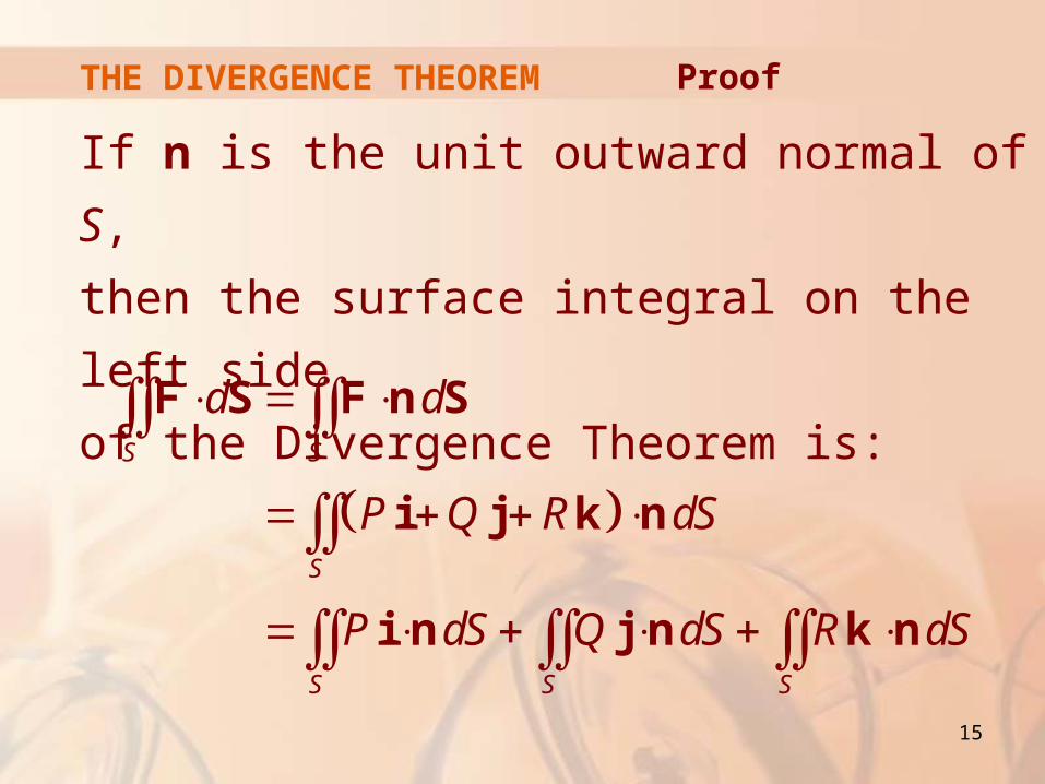
THE DIVERGENCE THEOREM
If n is the unit outward normal of S,
then the surface integral on the left side
of the Divergence Theorem is:
S S
S
S S S
d d
P Q R dS
P dS Q dS R dS
F S F n S
i j k n
i n j n k n
Proof
16
THE DIVERGENCE THEOREM
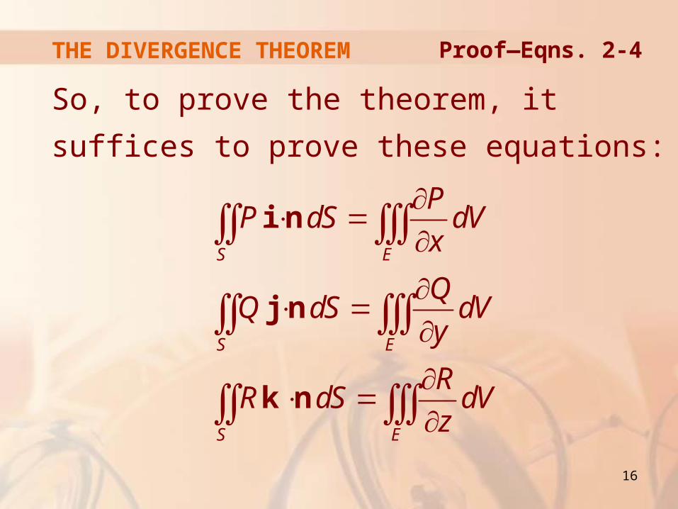
So, to prove the theorem, it suffices to prove
these equations:
S E
S E
S E
PP dS dV
x
QQ dS dV
y
RR dS dV
z
i n
j n
k n
Proof—Eqns. 2-4
17
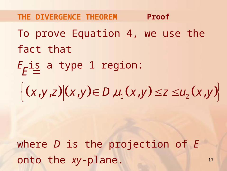
THE DIVERGENCE THEOREM
To prove Equation 4, we use the fact that
E is a type 1 region:
where D is the projection of E
onto the xy-plane.
1 2, , , , , ,
E
x y z x y D u x y z u x y
Proof
18
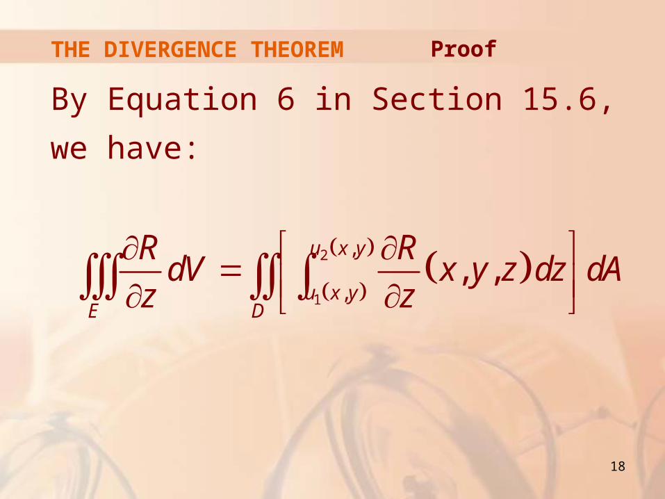
THE DIVERGENCE THEOREM
By Equation 6 in Section 15.6,
we have:
2
1
,
,, ,
u x y
u x yE D
R RdV x y z dz dAz z
Proof
19
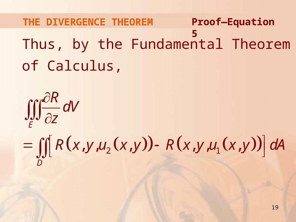
THE DIVERGENCE THEOREM
Thus, by the Fundamental Theorem of
Calculus,
2 1, , , , , ,
E
D
RdVz
R x y u x y R x y u x y dA
Proof—Equation 5
20
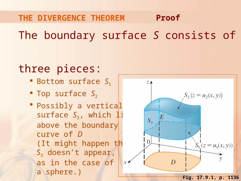
THE DIVERGENCE THEOREM
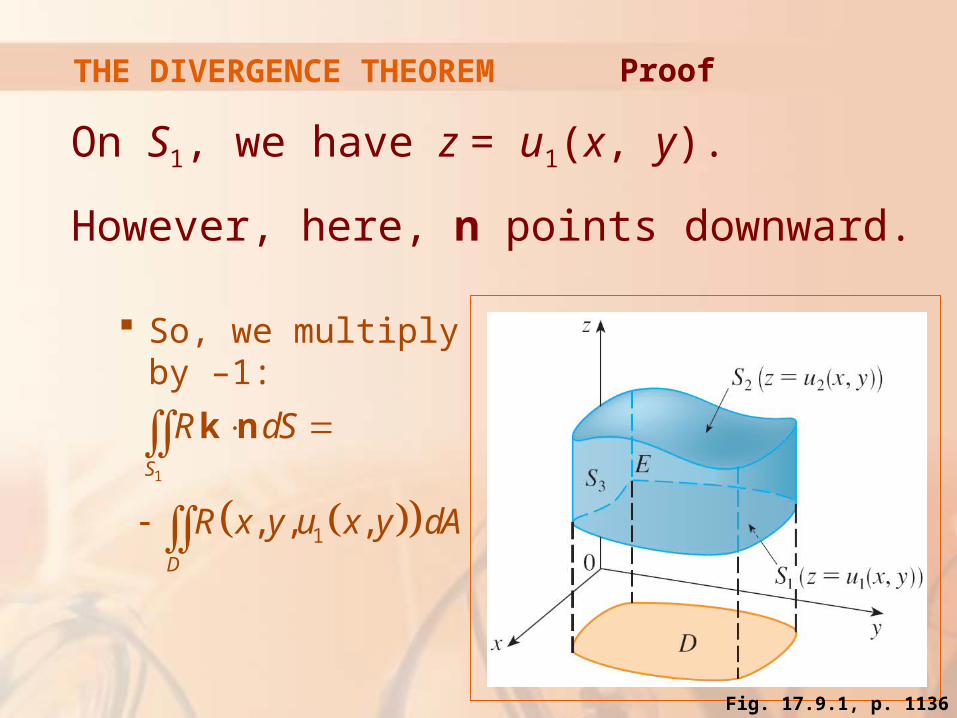
The boundary surface S consists of
three pieces: Bottom surface S1
Top surface S2
Possibly a vertical surface S3, which lies above the boundary curve of D(It might happen that S3 doesn’t appear, as in the case of a sphere.)
Proof
Fig. 17.9.1, p. 1136
21
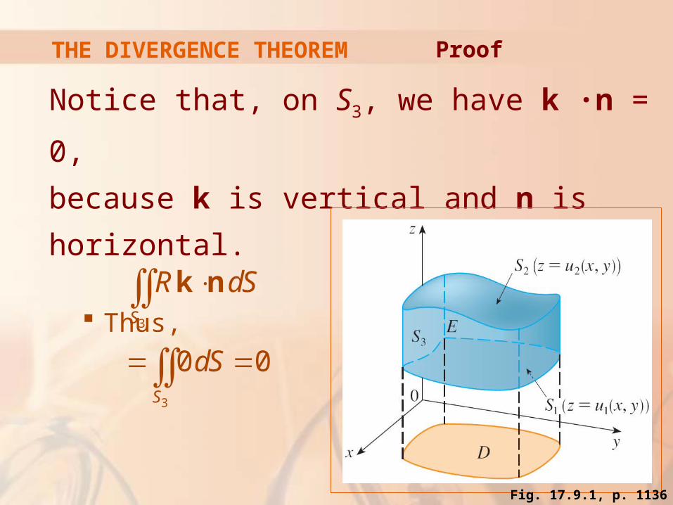
THE DIVERGENCE THEOREM
Notice that, on S3, we have k ∙n = 0,
because k is vertical and n is horizontal.
Thus,
Proof
3
3
0 0
S
S
R dS
dS
k n
Fig. 17.9.1, p. 1136
22
THE DIVERGENCE THEOREM
Thus, regardless of whether there is
a vertical surface, we can write:
1 2S S S
R dS R dS R dS k n k n k n
Proof—Equation 6
23
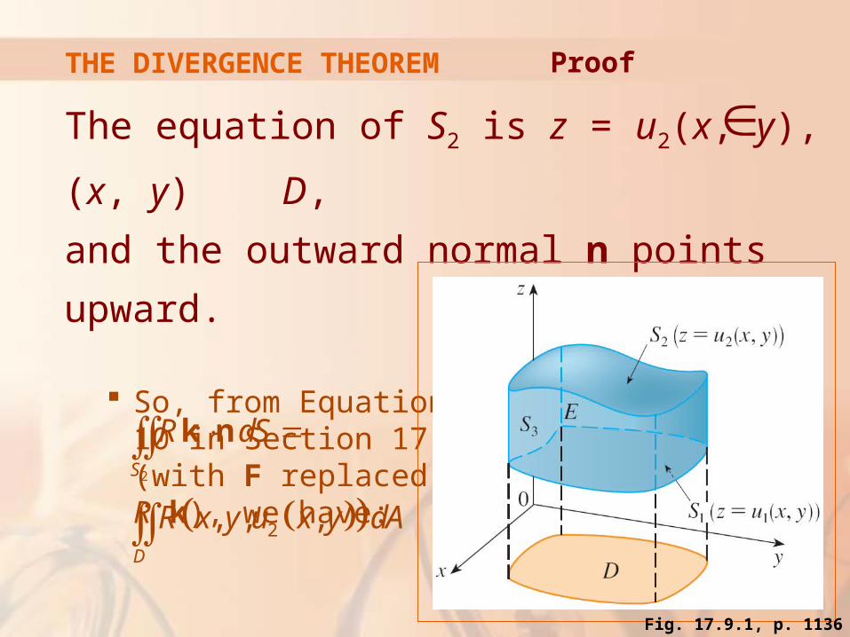
THE DIVERGENCE THEOREM
The equation of S2 is z = u2(x, y), (x, y) D,
and the outward normal n points upward.
So, from Equation 10 in Section 17.7 (with F replaced by R k), we have:
2
2, , ,
S
D
R dS
R x y u x y dA
k n
Proof
Fig. 17.9.1, p. 1136
24
THE DIVERGENCE THEOREM
On S1, we have z = u1(x, y).
However, here, n points downward.
So, we multiply by –1:
Proof
1
1, , ,
S
D
R dS
R x y u x y dA
k n
Fig. 17.9.1, p. 1136
25
THE DIVERGENCE THEOREM
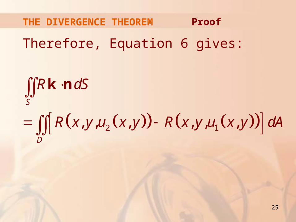
Therefore, Equation 6 gives:
2 1, , , , , ,
S
D
R dS
R x y u x y R x y u x y dA
k n
Proof
26
THE DIVERGENCE THEOREM
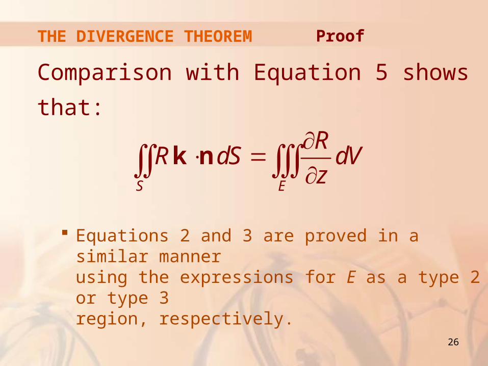
Comparison with Equation 5 shows
that:
Equations 2 and 3 are proved in a similar manner using the expressions for E as a type 2 or type 3 region, respectively.
S E
RR dS dV
z
k n
Proof
27
THE DIVERGENCE THEOREM
Notice that the method of proof of
the Divergence Theorem is very similar
to that of Green’s Theorem.
28
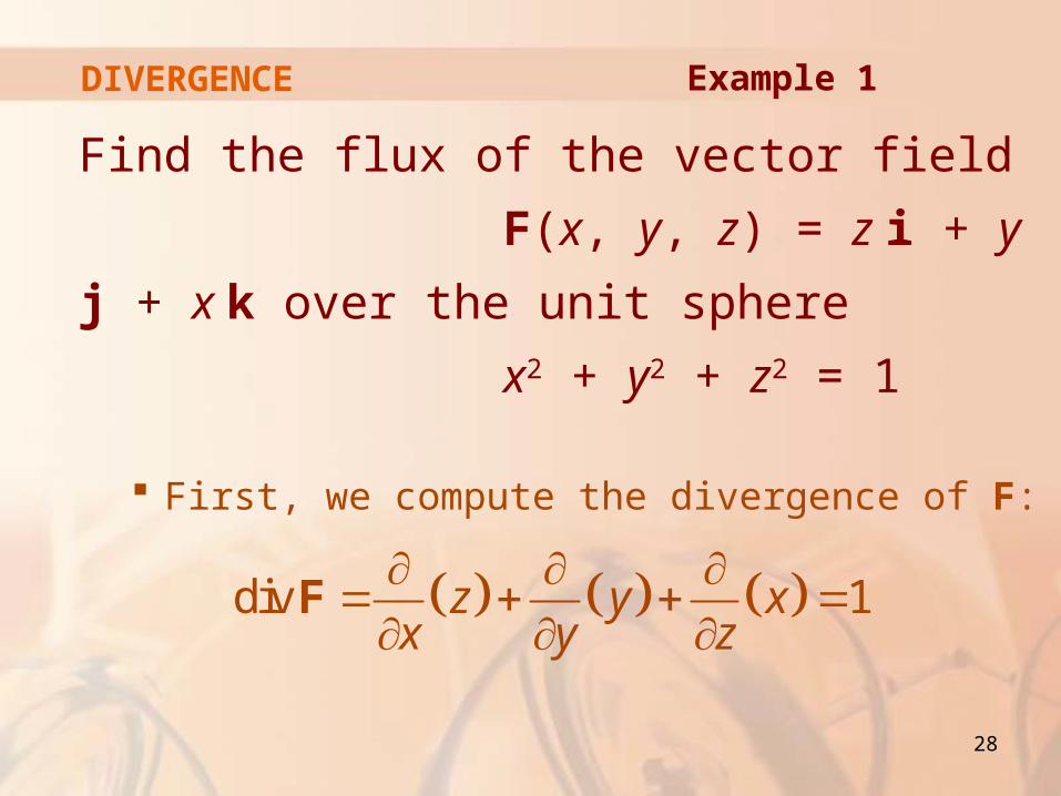
DIVERGENCE
Find the flux of the vector field
F(x, y, z) = z i + y j + x k
over the unit sphere
x2 + y2 + z2 = 1
First, we compute the divergence of F:
Example 1
div 1z y xx y z
F
29
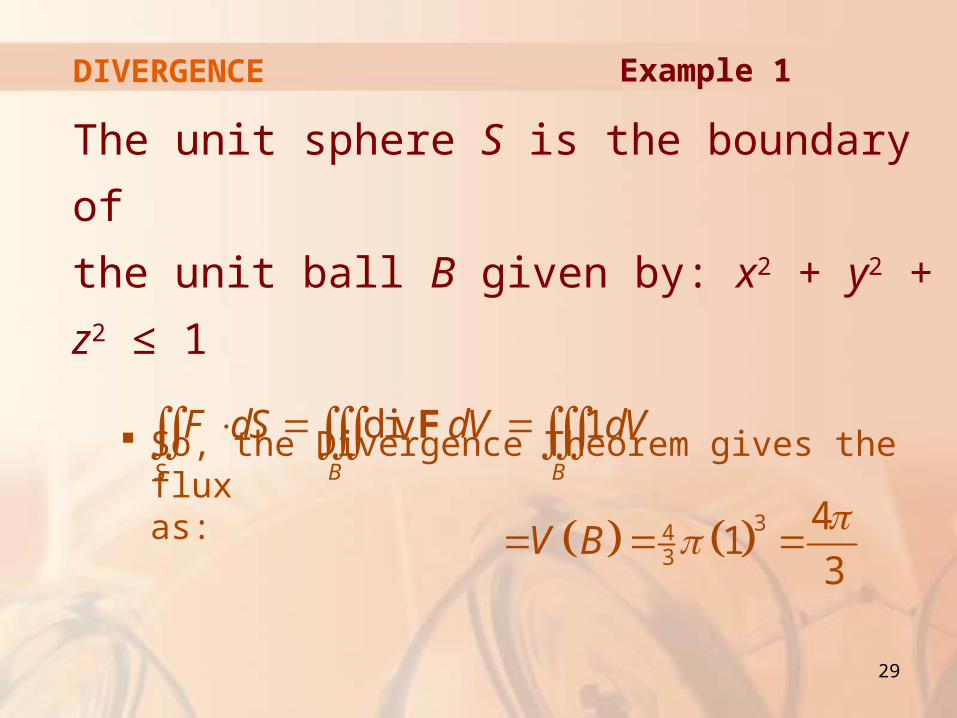
DIVERGENCE
The unit sphere S is the boundary of
the unit ball B given by: x2 + y2 + z2 ≤ 1
So, the Divergence Theorem gives the flux as:
343
div 1
41
3
S B B
F dS dV dV
V B
F
Example 1
30
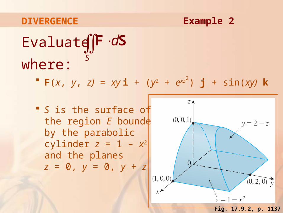
DIVERGENCE
Evaluate
where: F(x, y, z) = xy i + (y2 + exz2
) j + sin(xy) k
S is the surface of the region E bounded by the parabolic cylinder z = 1 – x2 and the planesz = 0, y = 0, y + z = 2
S
dF S
Example 2
Fig. 17.9.2, p. 1137
31
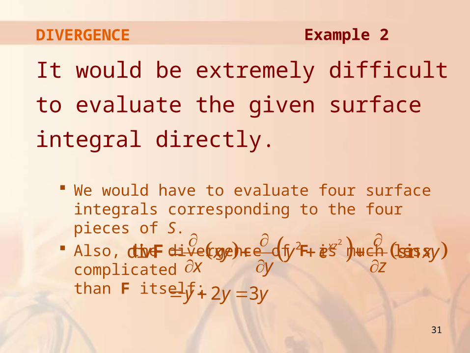
DIVERGENCE
It would be extremely difficult to evaluate
the given surface integral directly.
We would have to evaluate four surface integrals corresponding to the four pieces of S.
Also, the divergence of F is much less complicated than F itself:
Example 2
22div sin
2 3
xzxy y e xyx y z
y y y
F
32
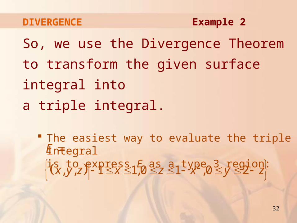
DIVERGENCE
So, we use the Divergence Theorem to
transform the given surface integral into
a triple integral.
The easiest way to evaluate the triple integral is to express E as a type 3 region:
2, , 1 1,0 1 ,0 2
E
x y z x z x y z
Example 2
33
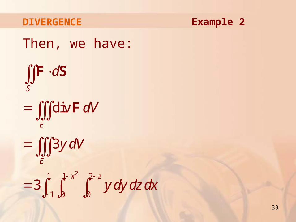
DIVERGENCE
Then, we have:
21 1 2
1 0 0
div
3
3
S
E
E
x z
d
dV
y dV
y dy dz dx
F S
F
Example 2
34
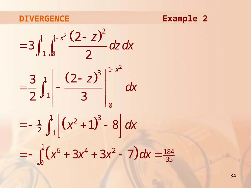
DIVERGENCE
2
2
21 1
1 0
131
1
0
1 3212 1
1 6 4 2 184350
23
2
23
2 3
1 8
3 3 7
x
x
zdz dx
zdx
x dx
x x x dx
Example 2
35
UNIONS OF SIMPLE SOLID REGIONS
The Divergence Theorem can also
be proved for regions that are finite
unions of simple solid regions.
The procedure is similar to the one we used in Section 17.4 to extend Green’s Theorem.
36
UNIONS OF SIMPLE SOLID REGIONS
For example, let’s consider the region E
that lies between the closed surfaces S1
and S2, where S1 lies inside S2.
Let n1 and n2 be outward normals of S1 and S2.
37
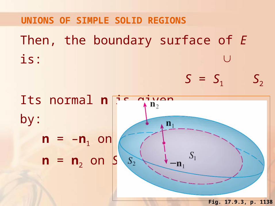
UNIONS OF SIMPLE SOLID REGIONS
Then, the boundary surface of E is:
S = S1 S2
Its normal n is given
by:
n = –n1 on S1
n = n2 on S2
Fig. 17.9.3, p. 1138
38
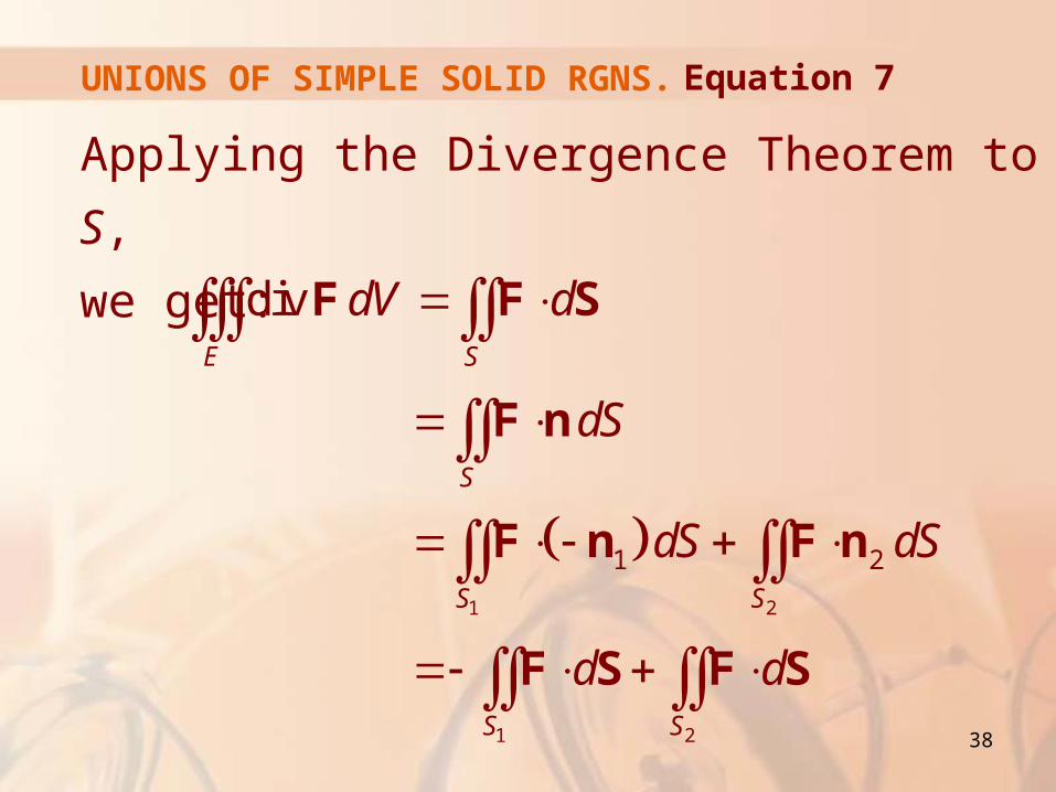
UNIONS OF SIMPLE SOLID RGNS.
Applying the Divergence Theorem to S,
we get:
1 2
1 2
1 2
divE S
S
S S
S S
dV d
dS
dS dS
d d
F F S
F n
F n F n
F S F S
Equation 7
39
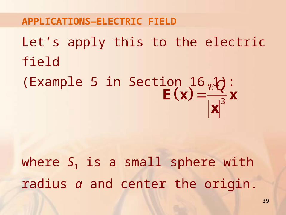
APPLICATIONS—ELECTRIC FIELD
Let’s apply this to the electric field
(Example 5 in Section 16.1):
where S1 is a small sphere with
radius a and center the origin.
3
QE x xx
40
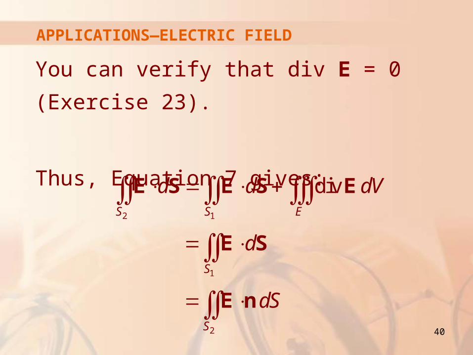
APPLICATIONS—ELECTRIC FIELD
You can verify that div E = 0 (Exercise 23).
Thus, Equation 7 gives:
2 1
1
2
divS S E
S
S
d d dV
d
dS
E S E S E
E S
E n

41
APPLICATIONS—ELECTRIC FIELD
The point of this calculation is that
we can compute the surface integral
over S1 because S1 is a sphere.
42
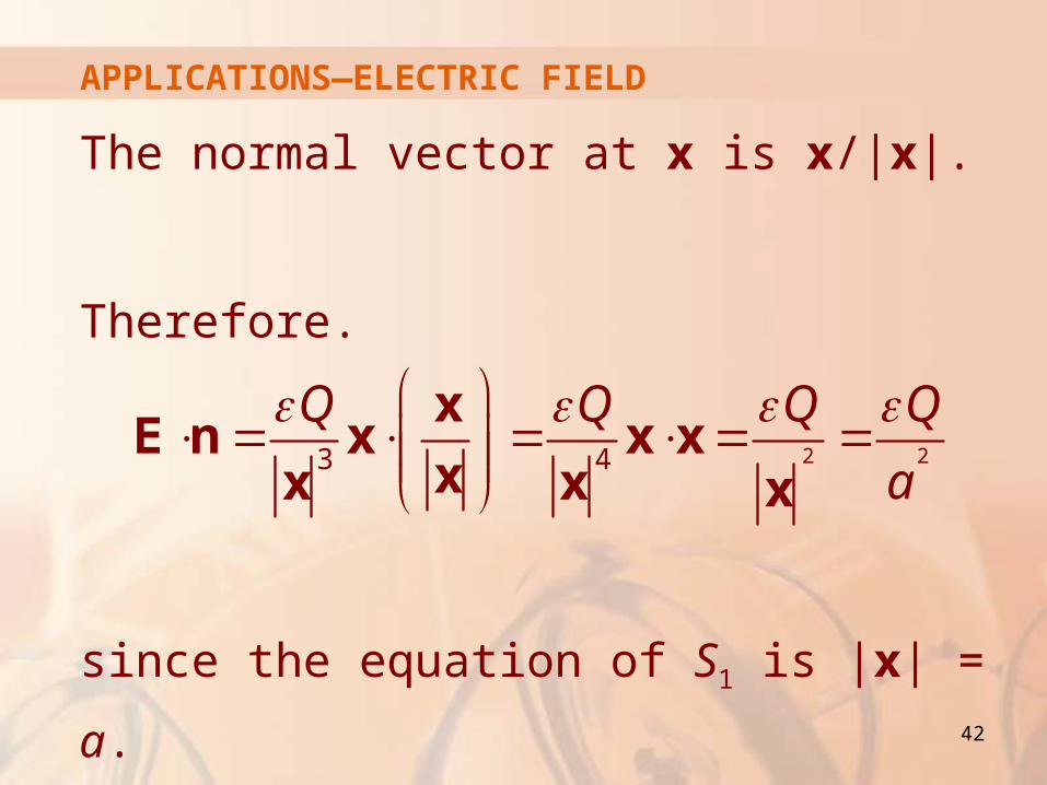
APPLICATIONS—ELECTRIC FIELD
The normal vector at x is x/|x|.
Therefore.
since the equation of S1 is |x| = a.
2 23 4
Q Q Q Q
a
xE n x x x
xx x x
43
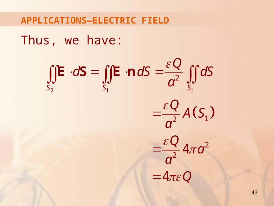
APPLICATIONS—ELECTRIC FIELD
Thus, we have:
2 1 1
2
12
224
4
S S S
Qd dS dS
a
QA S
aQ
aaQ
E S E n
44
APPLICATIONS—ELECTRIC FIELD
This shows that the electric flux of E is 4πεQ
through any closed surface S2 that contains
the origin.
This is a special case of Gauss’s Law (Equation 11 in Section 17.7) for a single charge.
The relationship between ε and ε0 is ε = 1/4πε0.
45
APPLICATIONS—FLUID FLOW
Another application of the Divergence
Theorem occurs in fluid flow.
Let v(x, y, z) be the velocity field of a fluid with constant density ρ.
Then, F = ρv is the rate of flow per unit area.
46
APPLICATIONS—FLUID FLOW
Suppose:
P0(x0, y0, z0) is a point in the fluid.
Ba is a ball with center P0 and very small
radius a.
Then, div F(P) ≈ div F(P0) for all points in Ba since div F is continuous.
47
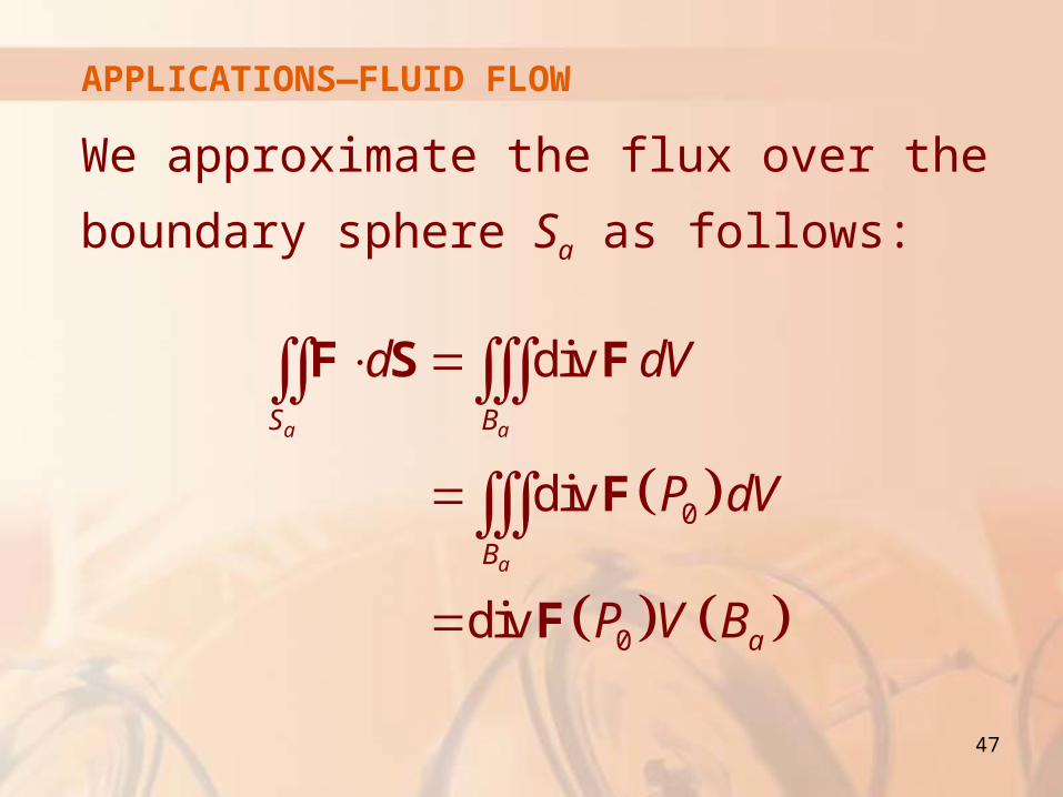
APPLICATIONS—FLUID FLOW
We approximate the flux over the boundary
sphere Sa as follows:
0
0
div
div
div
a a
a
S B
B
a
d dV
P dV
P V B
F S F
F
F
48
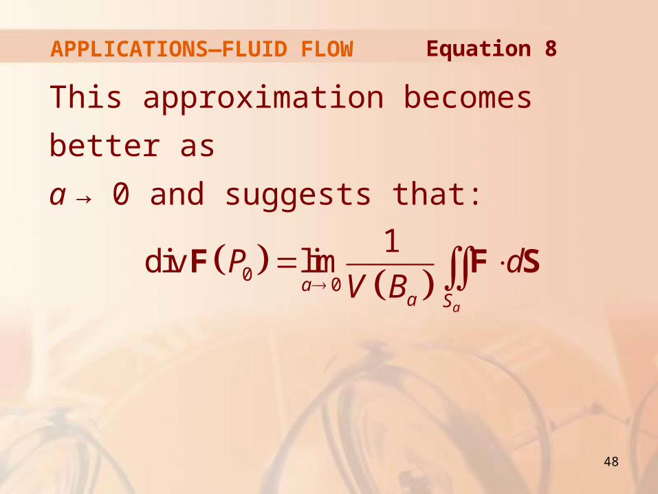
APPLICATIONS—FLUID FLOW
This approximation becomes better as
a → 0 and suggests that:
00
1div lim
a
aa S
P dV B
F F S
Equation 8
49
SOURCE AND SINK
Equation 8 says that div F(P0) is the net rate
of outward flux per unit volume at P0.
(This is the reason for the name divergence.)
If div F(P) > 0, the net flow is outward near P and P is called a source.
If div F(P) < 0, the net flow is inward near P and P is called a sink.
50
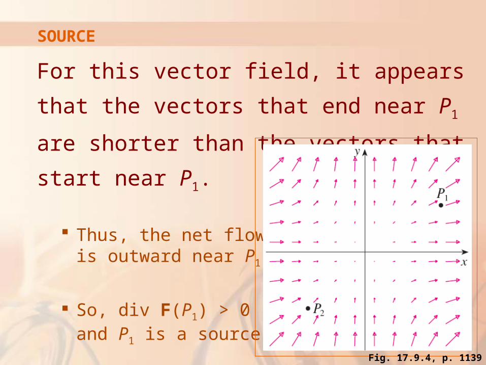
SOURCE
For this vector field, it appears that the vectors
that end near P1 are shorter than the vectors
that start near P1.
Thus, the net flow is outward near P1.
So, div F(P1) > 0 and P1 is a source.
Fig. 17.9.4, p. 1139
51
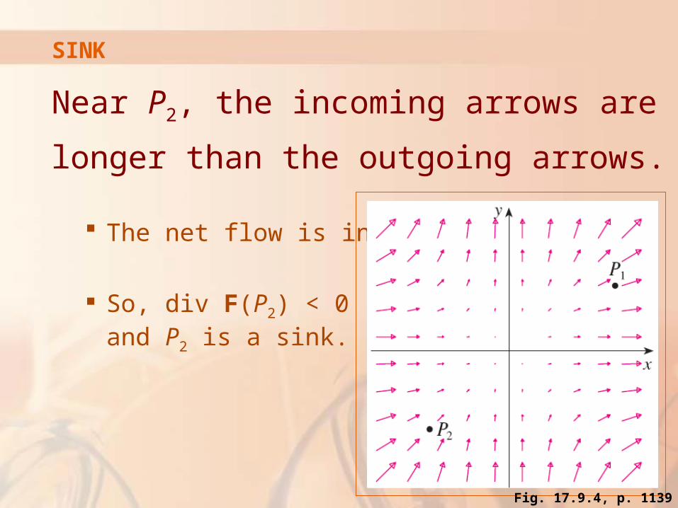
SINK
Near P2, the incoming arrows are longer
than the outgoing arrows.
The net flow is inward.
So, div F(P2) < 0 and P2 is a sink.
Fig. 17.9.4, p. 1139
52
SOURCE AND SINK
We can use the formula for F to confirm
this impression.
Since F = x2 i + y2 j, we have div F = 2x + 2y, which is positive when y > –x.
So, the points above the line y = –x are sources and those below are sinks.