Discrete Tomography by ContinuousMultilabeling Subject to Projection Constraints

Matthias Zisler, Stefania Petra, Claudius Schnorr, and Christoph Schnorr

Heidelberg University

Abstract. We present a non-convex variational approach to non-binarydiscrete tomography which combines non-local projection constraintswith a continuous convex relaxation of the multilabeling problem. Min-imizing this non-convex energy is achieved by a fixed point iterationwhich amounts to solving a sequence of convex problems, with guaran-teed convergence to a critical point. A competitive numerical evaluationusing standard test-datasets demonstrates a significantly improved re-construction quality for noisy measurements from a small number ofprojections.

1 Introduction

Computed tomography [14] deals after spatial discretization in an algebraic set-up with the reconstruction of 2D- or 3D-images u ∈ RN from a small number ofnoisy measurements b = Au + ν ∈ Rm. The latter correspond to line integralsthat sum up all absorptions over each ray transmitted through the object. Agiven projection matrix A ∈ Rm×N encodes this imaging geometry. Applicationsrange from medical imaging [3] to natural sciences and industrial applications,like non-destructive material testing [7]. Many situations require to keep thenumber of measurements as low as possible, which leads to a small number ofprojections and hence to a severely ill–posed reconstruction problem.

To cope with such problems, a common assumption in the field of discrete to-mography [8] concerns knowledge of a finite range of u ∈ LN , L := {c1, ..., cK} ⊂[0, 1], that is, u represents a piecewise constant function. Our main concern inthis paper is to effectively exploit the additional prior knowledge in terms of L,besides the projection constraints, in order to solve the discrete reconstructionproblem

Au = b s.t. ui ∈ L, ∀ i = 1, . . . , N, (1)

which generally is a NP-hard problem.Related work on discrete tomography considers either binary or non-binary

(multivalued) problems. The latter ones are considerably more involved.Regarding binary discrete tomography, Weber et al. [29, 21] proposed to com-

bine a quadratic program with a non-convex penalty which gradually enforcesbinary constraints. More recently, Kappes et al. [9] showed how a binary discretegraphical model and a sequence of s-t graph-cuts can be used to take into accountthe affine projection constraints and to recover high-quality reconstructions.

2 M. Zisler, S. Petra, C. Schnorr, C. Schnorr

Regarding non-binary discrete tomography, an extension of the latter ap-proach is not straightforward due to the nonlocal projection constraints. We-ber [27, Chapter 6] proposed a non-convex term for non-binary discrete tomog-raphy that we derive in a natural way in the present work. However, Weber’sapproach differs with respect to the data term for the projection constraints,regularization and optimization, and additionally requires parameter tuning.

Because u is assumed to be piecewise constant, an obvious approach is toconsider sparsity promoting priors. The authors of [23] proposed a dynamic pro-gramming approach for minimizing the `0-norm of the gradient. However, theset L of feasble intensities is not exploited. In the convex setting, the integralityconstraints are dropped and priors like the `1-norm or the total variation (TV)are used [22, 6, 5], with a postprocessing step to round the continuous solutionto a piecewise constant one. This approach connects discrete tomography andthe fast evolving field of compressive sensing with corresponding recovery guar-antees [5]. Again, however, the prior information of the range of the image tobe reconstructed is not involved in the optimization process. We focus next onmethods that make use of the set L during the reconstruction process.

Tuysuzoglu et al. [25] casted the non-binary discrete reconstruction probleminto a series of submodular binary problems within an α-expansion approachby linearizing the `2-fidelity term around an iteratively updated working point.This local approximation discards a lot of information, and a significantly largernumber of projections is required to get reasonable reconstructions. Maeda etal. [12] suggested a probabilistic formulation which couples a continuous recon-struction with the Potts model. Alternating optimization is applied to maximizethe a posteriori probability locally. However, there is no guarantee that thesealternating continuous and discrete block coordinate steps converge.

Ramlau et al. [10] investigated the theoretical regularization properties ofthe piecewise constant Mumford-Shah functional [13] applied to linear ill-posedproblems. In earlier work [19], they considered discrete tomography reconstruc-tion using this framework. The difficult geometric optimization of the partitionis carried out by a level-set approach and additionally the intensities L wereestimated in an alternating fashion. By contrast, our approach is based on aconvex relaxation of the perimeter regularization and the set L is assumed to beknown beforehand.

Varga et al. [26] suggested a heuristic algorithm which is adaptively comb-ing an energy formulation with a non-convex polynomial in order to steer thereconstruction towards the feasible values. Batenburg et al. [2] proposed the Dis-crete Algebraic Reconstruction Technique (DART) algorithm which starts with acontinuous reconstruction by a basic algebraic reconstruction method, followedby thresholding to ensure a piecewise constant function. These steps interleavedwith smoothing are iteratively repeated to refine the locations where u jumps.This heuristic approach yields good reconstructions in practice but cannot becharacterized by an objective function that is optimized.

We regard [2, 26] as state-of-the-art approaches for the experimental compar-ison.

Discrete Tomography by Continuous Multilabeling 3

Contributions. We present a novel variational approach to the discretetomography reconstruction problem in the general non-binary case. Contraryto existing work, we utilize both the non-local projection constraints and thefeasible set of intensities L in connection with an established convex relaxationof the multilabeling approach with a Potts prior. We show how the resultingnon-convex overall energy can be optimized efficiently by a fixed-point iterationwhich requires to solve a convex problem at each step. In this way, the derivationof our non-convex data and its local updates arise naturally. We also proposea suitable rounding procedure as post-processing step, because the integralityconstraints are relaxed. A comprehensive numerical evaluation demonstrates thesuperior reconstruction performance of our approach compared to related work.

2 Reconstruction by Constrained Multilabeling

In this section, we first reformulate the discrete reconstruction problem (1) asa constraint combinatorial multilabeling problem. Then we derive a tractablevariational approximation and suggest a proper rounding procedure.

2.1 Constrained Multilabeling Problem

We assume that there are less measurements than pixels m� N and hence thatthe discrete reconstruction problem (1) is ill-posed and requires regularization.A common choice is the Potts model [18], R(u) = ‖∇u‖0 := |{i | (∇u)i 6= 0}|for sparse gradient regularization which favours piecewise constant images. Inpresence of noisy measurements b, we use the more general constraints b(ε) ≤Au ≤ b(ε) instead of Au = b, where ε is an upper bound of the noise level. As aresult, the discrete reconstruction problem can be rewritten as

E(u) = λ · ‖∇u‖0 s.t. b(ε) ≤ Au ≤ b(ε) ∧ ui ∈ L ∀ i = 1...N. (2)

We refer to problem (2) as a constrained multilabeling problem with Potts regu-larization but point out that, from the viewpoint of graphical models, the systemof affine inequalities induces (very) high-order potentials. This high-order inter-action induced by the non-local constraints results in a non-standard labelingproblem which becomes intractable for discrete approaches and larger problemsizes. We adopt, therefore, the strategy of solving a sequence of convex relax-ations in order to minimize a non-convex energy, which properly approximatesthe original problem.

2.2 Approximate Variational Problem

Our starting point is the established convex relaxation of the multilabeling prob-lem [30, 11, 17]. Minimizing the energy in (3a) below with respect to z over theset of relaxed indicator vectors (3b) assigns to each given image pixel from u0

a label of the set L = {c1, . . . , cK}. The discretized total variation, weighted

4 M. Zisler, S. Petra, C. Schnorr, C. Schnorr

by λ, and the simplex constraints G constitute a basic convex relaxation of theintegrality constraints with respect to z.

E(z, u0) =

N∑i=1

K∑k=1

zik(u0i − ck

)2+ λ

K∑k=1

‖∇zk‖1 (3a)

s.t. z ∈ G :=

{z ∈ [0, 1]N×K :

K∑k=1

zik = 1, ∀ i = 1, . . . , N

}. (3b)

Regarding the notation, we denote by zk, k ∈ {1, . . . ,K} the k-th column vectorof z and by zik = (zk)i the entries of the matrix z.

Next, we add the projection constraints b ≤ Au ≤ b to the relaxed energy (3a)by transforming the indicator variables z back to their corresponding intensitieswith the linear operator W : G→ RN , z 7→

∑Kl=1 clzl which preserves convexity

of the resulting energy

E(z, u0) =

N∑i=1

K∑k=1

zik(u0i − ck

)2+ λ

K∑k=1

‖∇zk‖1

+ δRm+

(AWz − b) + δRm−

(AWz − b) + δG(z).

(4)

Note that the constraints b ≤ AWz ≤ b and z ∈ G are implemented by indicatorfunctions δRm

+and δRm

−.

In tomography, no image u0 is given, however. Therefore, we cannot dropthe unary data term in Eq. (4), since the constraints are feasible for all convexcombinations of prototypes ck. In other words, the constraints only constrain thevalue of a pixel but do not indicate how the indicator variables should realizethis value (similar to estimating a vector given only its magnitude).

A straightforward approach would be to start with some initial guess u0, e.g.computed using some another reconstruction method, followed by iterativelyapplying this approach above. This gives the fixed point iteration

zn+1 = arg minz

E(z,Wzn). (5)

At every iteration a convex problem has to be solved whose solution updates theunary data term. This raises the question whether the iteration converges andwhich overall energy is actually optimized?

To address these questions, we first eliminate u0 in a principled way. Notethat E(z, ·) in (4) is differentiable with respect to the second argument. Weinvoke Fermat’s (first order) optimality condition u∗ = Wz which says that theoptimal u∗ must be equal to the weighted average of the labels ck. Substitutingthis optimality condition back into the energy (4) results in the final version ofthe proposed energy which only depends on z,

E(z) =

N∑i=1

K∑k=1

zik ((Wz)i − ck)2

+ λ

K∑k=1

‖∇zk‖1

+ δRm+

(AWz − b) + δRm−

(AWz − b) + δG(z).

(6)

Discrete Tomography by Continuous Multilabeling 5

This new energy function, Eq. (6), is non-convex because of the products in thefirst term which measures the discreteness of z. We call this term phase dataterm and denote it by

D(z) :=

N∑i=1

K∑k=1

zik ((Wz)i − ck)2. (7)

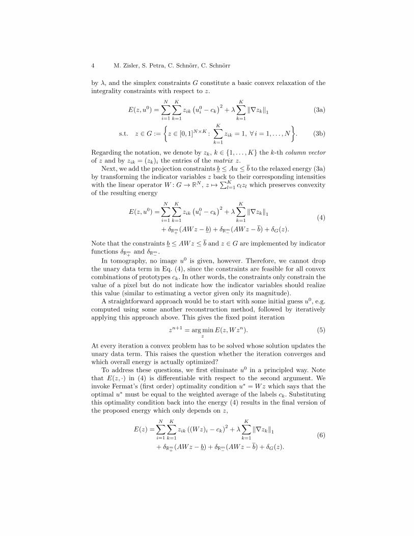
Fig. 1. Visualization of the phase data term D(z)for N = 1 over the probability simplex G, the ver-tices correspond to the values L = {0.0, 0.4, 1.0}.Note that the minimum is attained at the verticesof the simplex which correspond to unit vectors.

Using the notation introduced after Eq. (3), the i-th summand of (7) reads

K∑k=1

zik

( K∑l=1

zilcl − ck)2

=

K∑k=1

zikc2k −

( K∑k=1

zikck

)2(8)

which is concave with respect to the vector zi. Consequently, D(z) given by (7)is concave as well. Figure 1 shows a plot of D(z). Weber [27, Chapter 6] proposedthis term for discrete tomography which arises here in a natural way, whereas hisoverall approach differs with respect to data term for the projection constraints,regularization and optimization.

3 Optimization

In this section, we reformulate the objective function (6) as a DC program [15]and work out a corresponding optimization algorithm.

DC Programming. A large subclass of non-convex optimization problemsare DC functions (difference of convex functions) which can be solved by DCProgramming [15]. This generalizes subgradient optimization of convex functionsto local optimization of DC functions. Accordingly, basic concepts of convex op-timization like duality and KKT conditions were extended to DC functions [24].The basic form of a DC program is given by

z∗ = arg minz

g(z)− h(z), (9)

where g(z) and h(x) are proper, lower semicontinuous, convex functions. Thereexists a simplified version of the DC algorithm [16] for minimizing (9) whichguarantees convergence to a critical point by starting with z0 ∈ dom(g) andthen alternatingly applying the updates

vn ∈ ∂h(zn) and zn+1 ∈ ∂g∗(vn) (10)

6 M. Zisler, S. Petra, C. Schnorr, C. Schnorr

until a termination criterion is reached, where g∗ denotes the Legendre-Fenchelconjugate [20] of g. To apply the DC algorithm to our non-convex energy E(z) in(6), we rewrite E(z) = g(z)−h(z) as a DC function. We set h(z) = −D(z) sincethe phase data term (7) is concave by (8), and we denote by g(z) the remainingconvex terms from Eq. (6).

In order to make the step zn+1 ∈ ∂g∗(vn) explicit, we apply the subgradientinversion rule of convex analysis to obtain

zn+1 ∈ ∂g∗(vn) ⇔ vn ∈ ∂g(zn+1) ⇔ 0 ∈ ∂g(zn+1)− vn (11)

which is equivalent to the convex optimization problem

zn+1 = arg minz

g(z)− 〈vn, z〉. (12)

Because h is differentiable, the first step of (10) reads

vn ∈ ∂h(zn) ⇔ vn = −∇D(zn), (13)

where the gradient of D at z for pixel i and label ck is given by (see Lemma 1from the supplementary material)

(∇D(z))ik =∂D(z)

∂zik= ((Wz)i − ck)2, i = 1, . . . , N, k = 1, . . . ,K. (14)

Combining equations (13) and (14) and inserting into equation (12) yields

zn+1 = arg minz

E(z,Wzn) = arg minz

g(z) +

N∑i=1

K∑k=1

zik ((Wzn)i − ck)2. (15)

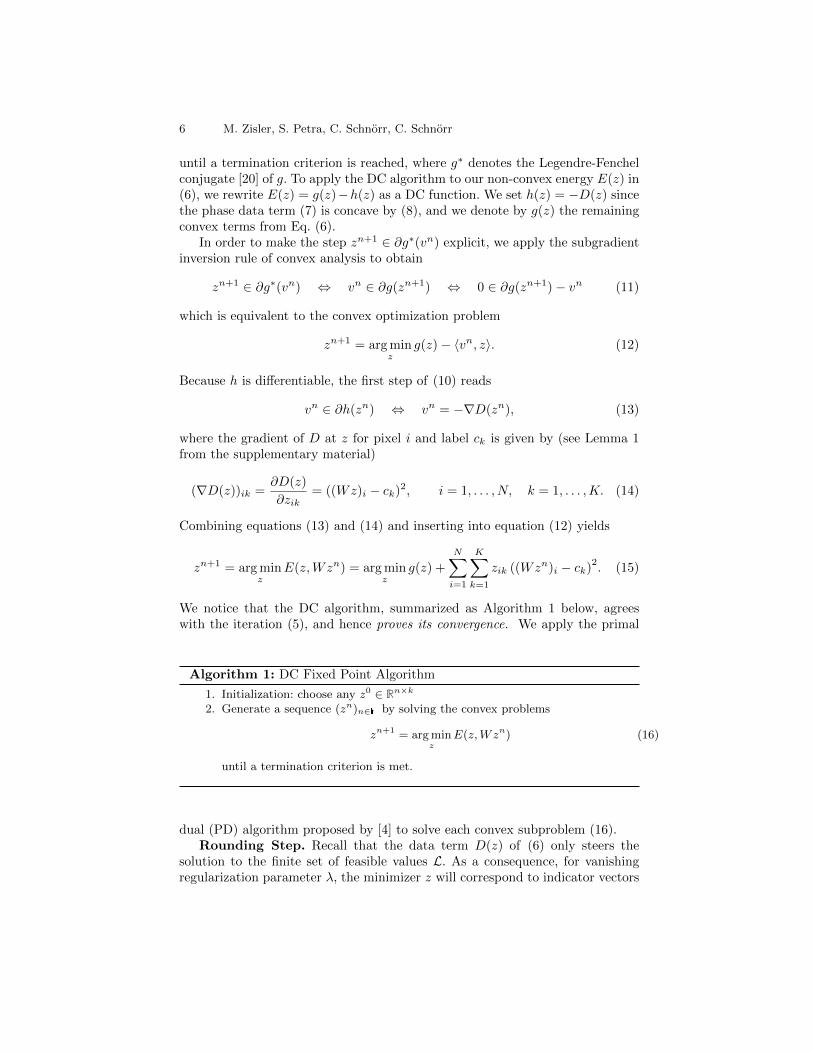
We notice that the DC algorithm, summarized as Algorithm 1 below, agreeswith the iteration (5), and hence proves its convergence. We apply the primal

Algorithm 1: DC Fixed Point Algorithm

1. Initialization: choose any z0 ∈ Rn×k

2. Generate a sequence (zn)n∈N by solving the convex problems

zn+1 = arg minz

E(z,Wzn) (16)

until a termination criterion is met.

dual (PD) algorithm proposed by [4] to solve each convex subproblem (16).Rounding Step. Recall that the data term D(z) of (6) only steers the

solution to the finite set of feasible values L. As a consequence, for vanishingregularization parameter λ, the minimizer z will correspond to indicator vectors

Discrete Tomography by Continuous Multilabeling 7

zi that assign a unique label to each pixel i. For larger values of λ which are morecommon in practice, however, the minimizing vectors zi will not be integral ingeneral. Therefore, a post-processing step for rounding the solution is required.

Given the minimizer z∗ of (6), we propose to select a label for each pixel ias a post-processing step by solving the local problems

u∗i = arg minc∈L

|(Wz∗)i − c|, i = 1, . . . , N. (17)

Note that this method differs from the common rounding procedure of multi-labeling approaches which select the label ck if zik = max{zi1, . . . , ziK}.

4 Numerical Experiments

Set-up. In this section, we compare our approach to state-of-the-art approachesfor non-binary discrete tomography in limited angles scenarios. Specifically, weconsidered the Discrete Algebraic Reconstruction Technique (DART ) [2] andthe energy minimization method from Varga et al. [26] (Varga). As multivalued

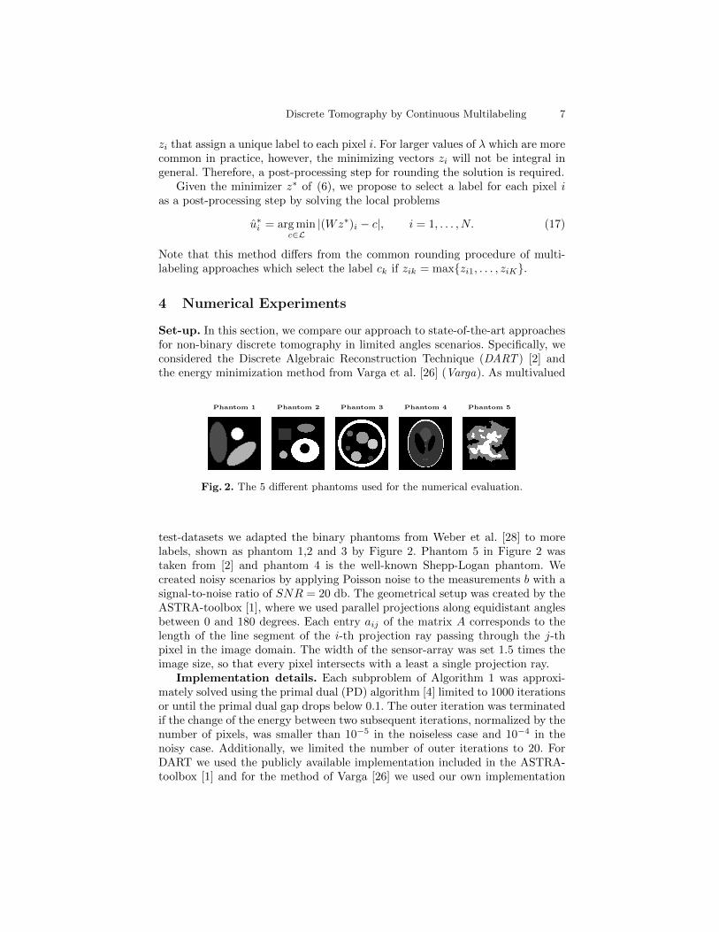
Phantom 1 Phantom 2 Phantom 3 Phantom 4 Phantom 5

Fig. 2. The 5 different phantoms used for the numerical evaluation.

test-datasets we adapted the binary phantoms from Weber et al. [28] to morelabels, shown as phantom 1,2 and 3 by Figure 2. Phantom 5 in Figure 2 wastaken from [2] and phantom 4 is the well-known Shepp-Logan phantom. Wecreated noisy scenarios by applying Poisson noise to the measurements b with asignal-to-noise ratio of SNR = 20 db. The geometrical setup was created by theASTRA-toolbox [1], where we used parallel projections along equidistant anglesbetween 0 and 180 degrees. Each entry aij of the matrix A corresponds to thelength of the line segment of the i-th projection ray passing through the j-thpixel in the image domain. The width of the sensor-array was set 1.5 times theimage size, so that every pixel intersects with a least a single projection ray.

Implementation details. Each subproblem of Algorithm 1 was approxi-mately solved using the primal dual (PD) algorithm [4] limited to 1000 iterationsor until the primal dual gap drops below 0.1. The outer iteration was terminatedif the change of the energy between two subsequent iterations, normalized by thenumber of pixels, was smaller than 10−5 in the noiseless case and 10−4 in thenoisy case. Additionally, we limited the number of outer iterations to 20. ForDART we used the publicly available implementation included in the ASTRA-toolbox [1] and for the method of Varga [26] we used our own implementation

8 M. Zisler, S. Petra, C. Schnorr, C. Schnorr

Proposednoiseless

Proposednoise case

DART[2]noiseless

DART[2]noise case

Varga[26]noiseless

Varga[26]noise case

2

3

7

10

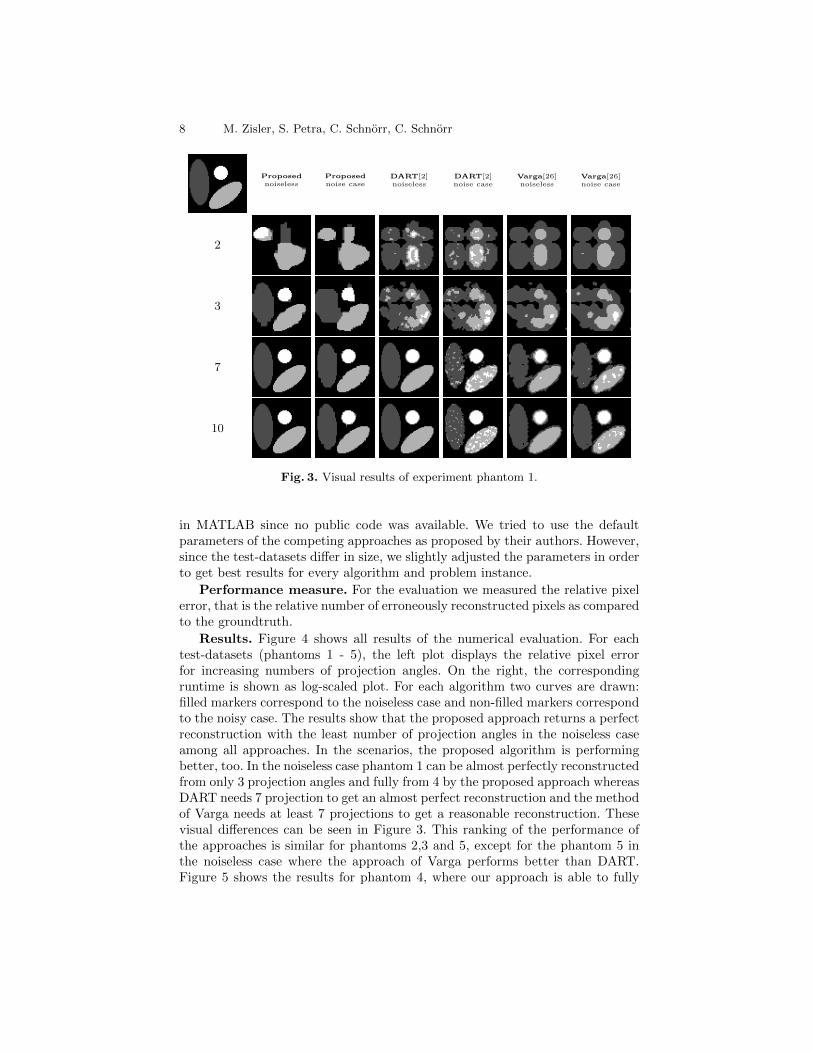
Fig. 3. Visual results of experiment phantom 1.

in MATLAB since no public code was available. We tried to use the defaultparameters of the competing approaches as proposed by their authors. However,since the test-datasets differ in size, we slightly adjusted the parameters in orderto get best results for every algorithm and problem instance.

Performance measure. For the evaluation we measured the relative pixelerror, that is the relative number of erroneously reconstructed pixels as comparedto the groundtruth.

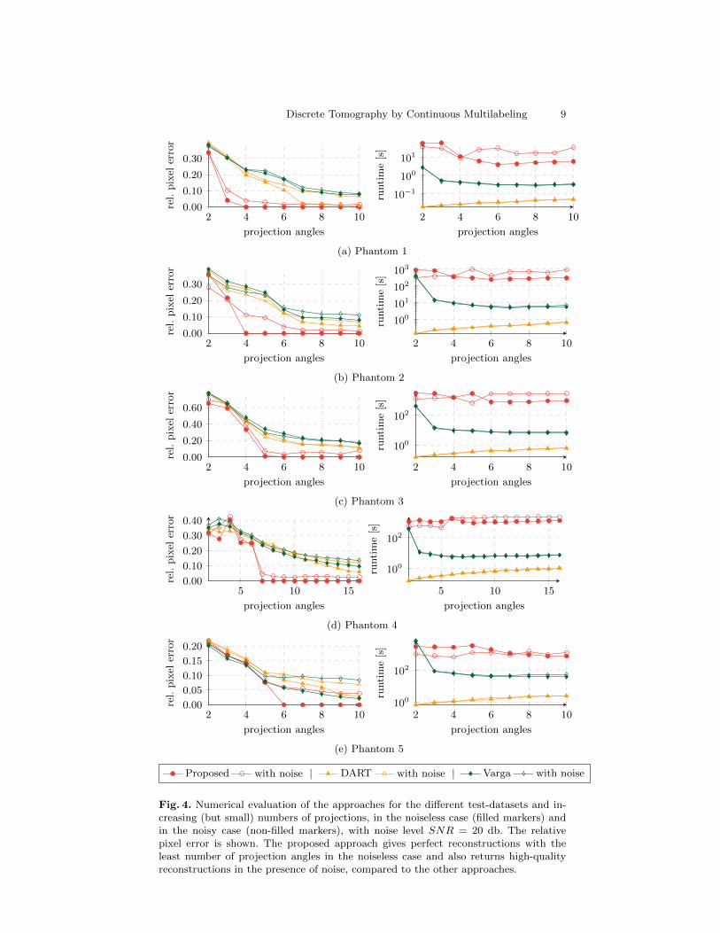
Results. Figure 4 shows all results of the numerical evaluation. For eachtest-datasets (phantoms 1 - 5), the left plot displays the relative pixel errorfor increasing numbers of projection angles. On the right, the correspondingruntime is shown as log-scaled plot. For each algorithm two curves are drawn:filled markers correspond to the noiseless case and non-filled markers correspondto the noisy case. The results show that the proposed approach returns a perfectreconstruction with the least number of projection angles in the noiseless caseamong all approaches. In the scenarios, the proposed algorithm is performingbetter, too. In the noiseless case phantom 1 can be almost perfectly reconstructedfrom only 3 projection angles and fully from 4 by the proposed approach whereasDART needs 7 projection to get an almost perfect reconstruction and the methodof Varga needs at least 7 projections to get a reasonable reconstruction. Thesevisual differences can be seen in Figure 3. This ranking of the performance ofthe approaches is similar for phantoms 2,3 and 5, except for the phantom 5 inthe noiseless case where the approach of Varga performs better than DART.Figure 5 shows the results for phantom 4, where our approach is able to fully

Discrete Tomography by Continuous Multilabeling 9

2 4 6 8 100.00

0.10

0.20

0.30

projection angles

rel.

pix

eler

ror

2 4 6 8 10

10−1

100

101

projection angles

runti

me

[s]

(a) Phantom 1

2 4 6 8 100.00

0.10

0.20

0.30

projection angles

rel.

pix

eler

ror

2 4 6 8 10

100

101

102

103

projection angles

runti

me

[s]

(b) Phantom 2

2 4 6 8 100.00

0.20

0.40

0.60

projection angles

rel.

pix

eler

ror

2 4 6 8 10

100

102

projection angles

runti

me

[s]

(c) Phantom 3

5 10 150.00

0.10

0.20

0.30

0.40

projection angles

rel.

pix

eler

ror

5 10 15

100

102

projection angles

runti

me

[s]

(d) Phantom 4

2 4 6 8 100.00

0.05

0.10

0.15

0.20

projection angles

rel.

pix

eler

ror

2 4 6 8 10100

102

projection angles

runti

me

[s]

(e) Phantom 5

Proposed with noise | DART with noise | Varga with noise

Fig. 4. Numerical evaluation of the approaches for the different test-datasets and in-creasing (but small) numbers of projections, in the noiseless case (filled markers) andin the noisy case (non-filled markers), with noise level SNR = 20 db. The relativepixel error is shown. The proposed approach gives perfect reconstructions with theleast number of projection angles in the noiseless case and also returns high-qualityreconstructions in the presence of noise, compared to the other approaches.

10 M. Zisler, S. Petra, C. Schnorr, C. Schnorr

Proposednoiseless

Proposednoise case

DART[2]noiseless

DART[2]noise case

Varga[26]noiseless

Varga[26]noise case

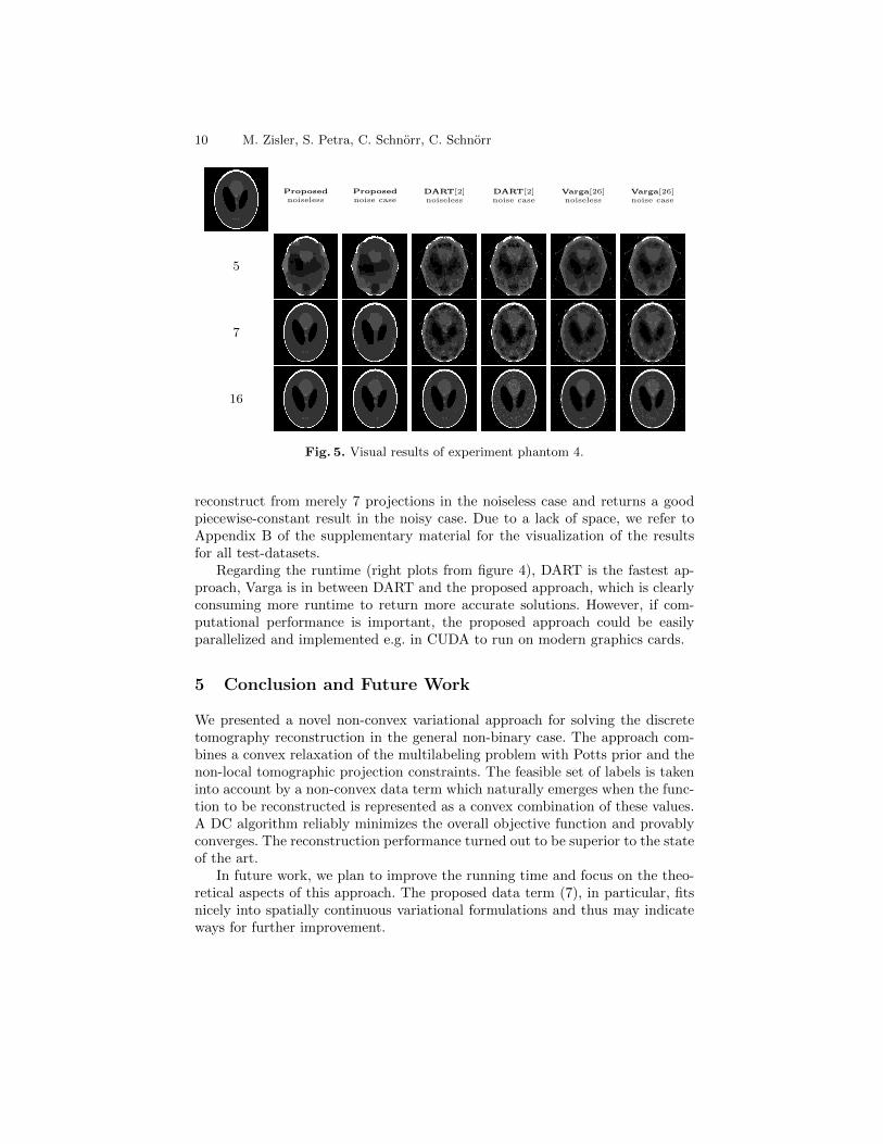
5

7

16

Fig. 5. Visual results of experiment phantom 4.

reconstruct from merely 7 projections in the noiseless case and returns a goodpiecewise-constant result in the noisy case. Due to a lack of space, we refer toAppendix B of the supplementary material for the visualization of the resultsfor all test-datasets.

Regarding the runtime (right plots from figure 4), DART is the fastest ap-proach, Varga is in between DART and the proposed approach, which is clearlyconsuming more runtime to return more accurate solutions. However, if com-putational performance is important, the proposed approach could be easilyparallelized and implemented e.g. in CUDA to run on modern graphics cards.

5 Conclusion and Future Work

We presented a novel non-convex variational approach for solving the discretetomography reconstruction in the general non-binary case. The approach com-bines a convex relaxation of the multilabeling problem with Potts prior and thenon-local tomographic projection constraints. The feasible set of labels is takeninto account by a non-convex data term which naturally emerges when the func-tion to be reconstructed is represented as a convex combination of these values.A DC algorithm reliably minimizes the overall objective function and provablyconverges. The reconstruction performance turned out to be superior to the stateof the art.

In future work, we plan to improve the running time and focus on the theo-retical aspects of this approach. The proposed data term (7), in particular, fitsnicely into spatially continuous variational formulations and thus may indicateways for further improvement.

Discrete Tomography by Continuous Multilabeling 11

References

1. Aarle, W., Palenstijn, W., Beenhouwer, J., Altantzis, T., Bals, S., Batenburg, K.,Sijbers, J.: The {ASTRA} Toolbox: A Platform for Advanced Algorithm Develop-ment in Electron Tomography. Ultramicroscopy 157, 35 – 47 (2015)

2. Batenburg, K., Sijbers, J.: DART: A Practical Reconstruction Algorithm for Dis-crete Tomography. Image Processing, IEEE Transactions on 20(9), 2542–2553 (Sept2011)

3. Bushberg, J., Seibert, J., Leidholdt, E., Boone, J.: The Essential Physics of MedicalImaging. Wolters Kluwer, 3rd edn. (2011)

4. Chambolle, A., Pock, T.: A First-Order Primal-Dual Algorithm for Convex Prob-lems with Applications to Imaging. J. Math. Imaging Vis. 40(1), 120–145 (May2011)

5. Denitiu, A., Petra, S., Schnorr, C., Schnorr, C.: Phase Transitions and CosparseTomographic Recovery of Compound Solid Bodies from Few Projections. Funda-menta Informaticae 135, 73–102 (2014)

6. Goris, B., Broek, W., Batenburg, K., Mezerji, H., Bals, S.: Electron Tomogra-phy Based on a Total Variation Minimization Reconstruction Technique. Ultrami-croscopy 113, 120 – 130 (2012)

7. Hanke, R., Fuchs, T., Uhlmann, N.: X-ray Based Methods for Non-DestructiveTesting and Material Characterization. Nuclear Instruments and Methods inPhysics Research Section A: Accelerators, Spectrometers, Detectors and Associ-ated Equipment 591(1), 14 – 18 (2008)

8. Herman, G., Kuba, A.: Discrete Tomography: Foundations, Algorithms and Ap-plications. Birkhauser (1999)

9. Kappes, J.H., Petra, S., Schnorr, C., Zisler, M.: TomoGC: Binary Tomography byConstrained GraphCuts. Proc. GCPR 30

10. Klann, E., Ramlau, R.: Regularization Properties of Mumford–Shah-Type Func-tionals with Perimeter and Norm Constraints for Linear Ill-Posed Problems. SIAMJournal on Imaging Sciences 6(1), 413–436 (2013)

11. Lellmann, J., Becker, F., Schnorr, C.: Convex Optimization for Multi-Class ImageLabeling with a Novel Family of Total Variation Based Regularizers. In: Proceed-ings of the IEEE Conference on Computer Vision (ICCV 09) Kyoto, Japan. pp.646–653 (2009), 1

12. Maeda, S., Fukuda, W., Kanemura, A., Ishii, S.: Maximum a posteriori X-raycomputed tomography using graph cuts. Journal of Physics: Conference Series 233(2010)

13. Mumford, D., Shah, J.: Optimal Approximations by Piecewise Smooth Functionsand Associated Variational Problems. Communications on Pure and Applied Math-ematics 42(5), 577–685 (1989)

14. Natterer, F., Wubbeling, F.: Mathematical Methods in Image Reconstruction.SIAM (2001)

15. Pham Dinh, T., El Bernoussi, S.: Algorithms for Solving a Class of Nonconvex Opti-mization Problems. Methods of Subgradients. In: Hiriart-Urruty, J.B. (ed.) FermatDays 85: Mathematics for Optimization, North-Holland Mathematics Studies, vol.129, pp. 249 – 271. North-Holland (1986)

16. Pham Dinh, T., Hoai An, L.: Convex Analysis Approach to D.C. Programming:Theory, Algorithms and Applications. Acta Math. Vietnamica 22(1), 289–355(1997)

12 M. Zisler, S. Petra, C. Schnorr, C. Schnorr

17. Pock, T., Chambolle, A., Cremers, D., Bischof, H.: A Convex Relaxation Approachfor Computing Minimal Partitions. In: Computer Vision and Pattern Recognition,2009. CVPR 2009. IEEE Conference on. pp. 810–817 (June 2009)

18. Potts, R.B.: Some Generalized Order-Disorder Transformations. MathematicalProceedings of the Cambridge Philosophical Society 48, 106–109 (1 1952)

19. Ramlau, R., Ring, W.: A Mumford–Shah Level-Set Approach for the Inversionand Segmentation of X-ray Tomography Data. Journal of Computational Physics221(2), 539–557 (2007)

20. Rockafellar, R.T., Wets, R.J.B.: Variational Analysis, vol. 317. Springer Science &Business Media (2009)

21. Schule, T., Schnorr, C., Weber, S., Hornegger, J.: Discrete Tomography by Convex-Concave Regularization and D.C. Programming. Discrete Applied Mathematics151(13), 229 – 243 (2005)

22. Sidky, E.Y., Pan, X.: Image Reconstruction in Circular Cone-Beam ComputedTomography by Constrained, Total-Variation Minimization. Physics in Medicineand Biology 53(17), 4777 (2008)

23. Storath, M., Weinmann, A., Frikel, J., Unser, M.: Joint Image Reconstruction andSegmentation Using the Potts Model. Inverse Problems 31(2), 025003 (2015)

24. Toland, J.F.: Duality in Nonconvex Optimization. Journal of Mathematical Anal-ysis and Applications 66(2), 399–415 (1978)

25. Tuysuzoglu, A., Karl, W., Stojanovic, I., Castanon, D., Unlu, M.: Graph-Cut BasedDiscrete-Valued Image Reconstruction. Image Processing, IEEE Transactions on24(5), 1614–1627 (May 2015)

26. Varga, L., Balazs, P., Nagy, A.: An Energy Minimization Reconstruction Algorithmfor Multivalued Discrete Tomography. In: 3rd International Symposium on Com-putational Modeling of Objects Represented in Images, Rome, Italy, Proceedings(Taylor & Francis). pp. 179–185 (2012)

27. Weber, S.: Discrete Tomography by Convex-Concave Regularization Using Linearand Quadratic Optimization. PhD thesis, Ruprecht-Karls-Universitat, Heidelberg,Germany (2009)

28. Weber, S., Nagy, A., Schule, T., Schnorr, C., Kuba, A.: A Benchmark Evaluation ofLarge-Scale Optimization Approaches to Binary Tomography. In: Discrete Geom-etry for Computer Imagery (DGCI 2006). LNCS, vol. 4245, pp. 146–156. Springer(2006)

29. Weber, S., Schnorr, C., Hornegger, J.: A Linear Programming Relaxation for Bi-nary Tomography with Smoothness Priors. Electronic Notes in Discrete Mathe-matics 12, 243–254 (2003)

30. Zach, C., Gallup, D., Frahm, J., Niethammer, M.: Fast Global Labeling for Real-Time Stereo Using Multiple Plane Sweeps. In: Proceedings of the Vision, Modeling,and Visualization Conference 2008, VMV 2008, Konstanz, Germany, October 8-10,2008. pp. 243–252 (2008)