1

Introduction to Inverse Problems (2 lectures)

Summary

Direct and inverse problems

Examples of direct (forward) problems

Deterministic and statistical points of view

Ill-posed and ill-conditioned problems

An illustrative example: The deconvolution problem

Truncated Fourier decomposition (TFD); Tikhonov regularization

Generalized Tikhonov regularization; Bayesian perspective.

Iterative optimization.

IP, José Bioucas Dias, 2007, IST

2

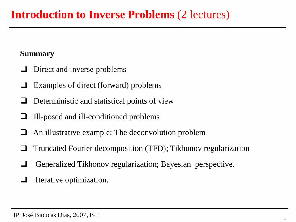
Direct/Inverse problems

Causes Effects

Direct (forward) problem

Inverse problem

Example:

Direct problem: the computation of the trajectories of bodies from the

knowledge of the forces.

Inverse problem: determination of the forces from the knowledge of the

trajectories

Newton solved the first direct/inverse problem: the determintion of the

gravitation force from the Kepler laws describing the trajectories of planets

3

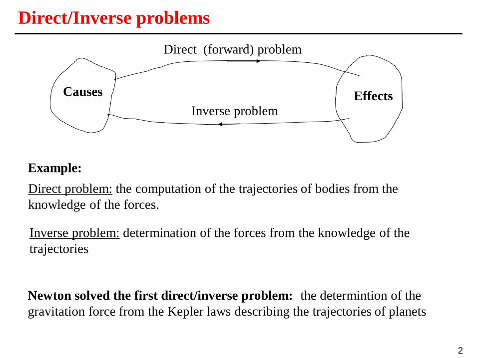
An example: a linear time invariant (LTI) system

Inverse problem:

Fourier domain

high frequencies of the

perturbation are amplified,

degrading the estimate of f

A perturbation on leads to a perturbation on given by

Source of difficulties: is unbounded

Direct problem:

4

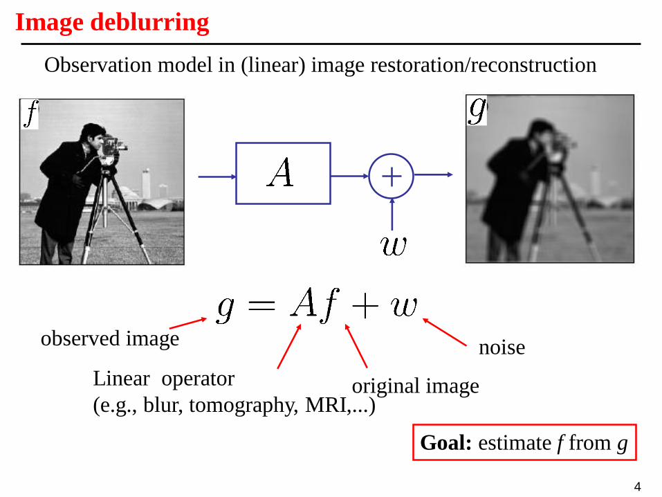
Image deblurring

Observation model in (linear) image restoration/reconstruction

observed image

original image

noise

Linear operator

(e.g., blur, tomography, MRI,...)

Goal: estimate f from g

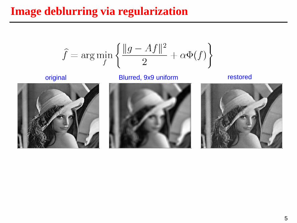
5

original restoredBlurred, 9x9 uniform

Image deblurring via regularization

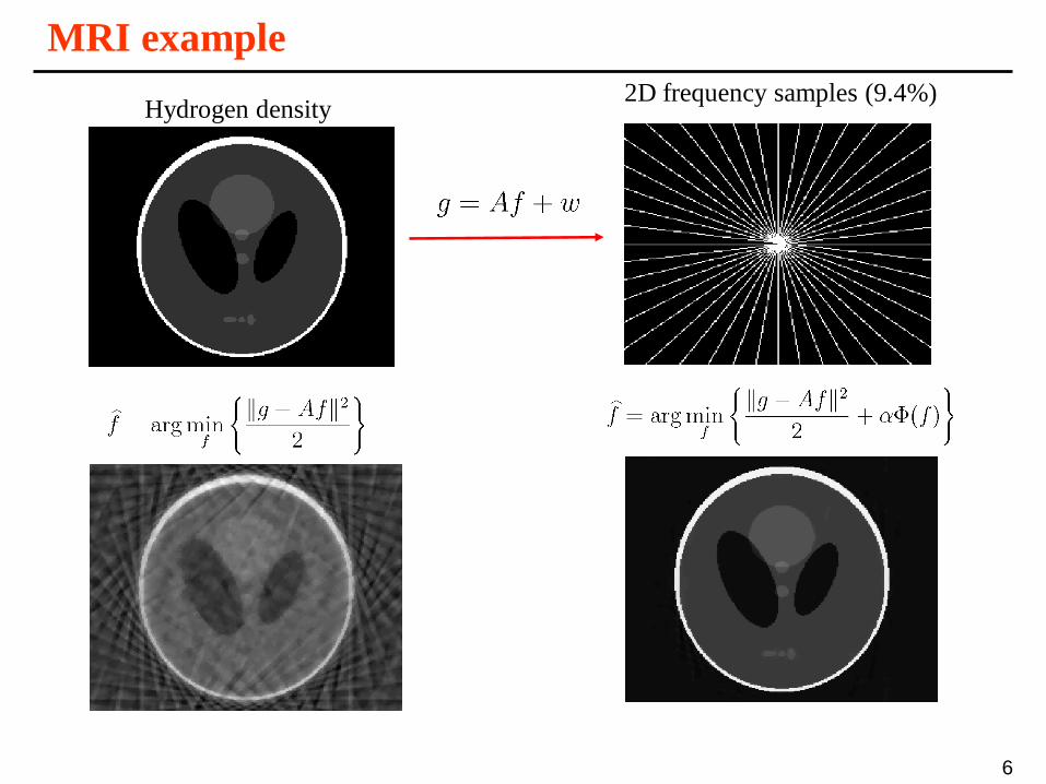
6

MRI example

Hydrogen density2D frequency samples (9.4%)

7

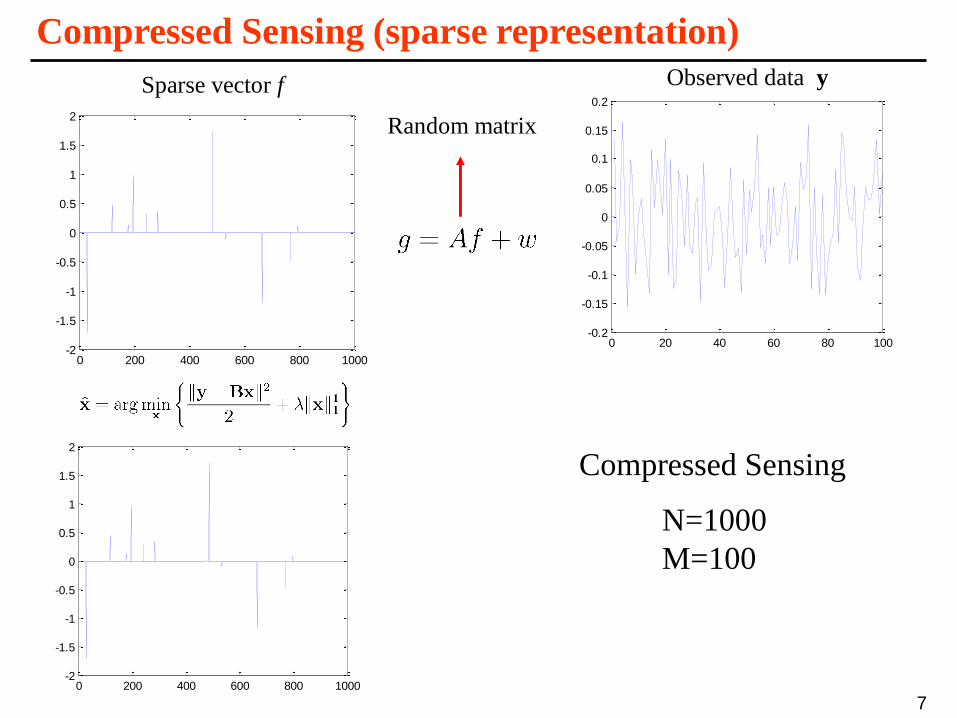
Compressed Sensing (sparse representation)

0 200 400 600 800 1000-2

-1.5

-1

-0.5

0

0.5

1

1.5

2

Sparse vector f

0 20 40 60 80 100-0.2

-0.15

-0.1

-0.05

0

0.05

0.1

0.15

0.2

Observed data y

Random matrix

0 200 400 600 800 1000-2

-1.5

-1

-0.5

0

0.5

1

1.5

2

N=1000

M=100

Compressed Sensing

8

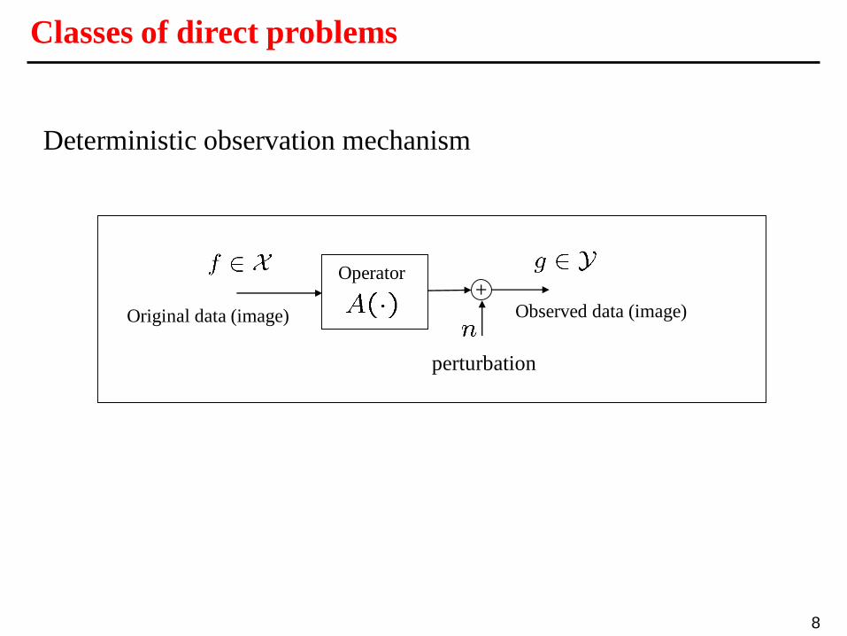
Deterministic observation mechanism

Classes of direct problems

+

perturbation

Operator

Original data (image) Observed data (image)

9

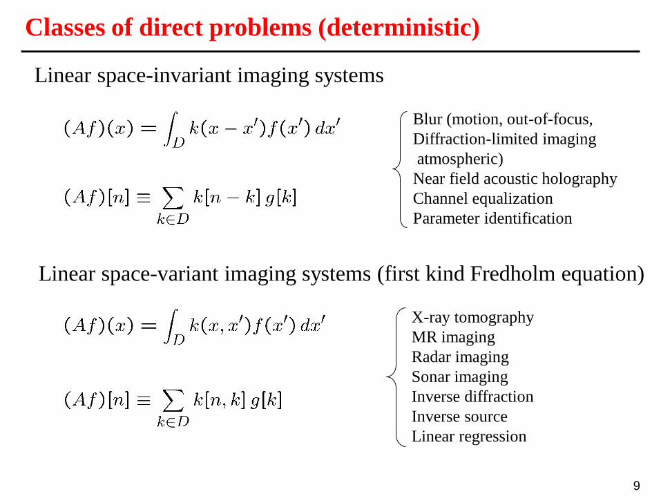
Classes of direct problems (deterministic)

Linear space-variant imaging systems (first kind Fredholm equation)

X-ray tomography

MR imaging

Radar imaging

Sonar imaging

Inverse diffraction

Inverse source

Linear regression

Blur (motion, out-of-focus,

Diffraction-limited imaging

atmospheric)

Near field acoustic holography

Channel equalization

Parameter identification

Linear space-invariant imaging systems

10

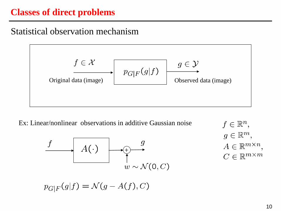
Classes of direct problems

Statistical observation mechanism

Original data (image) Observed data (image)

+

Ex: Linear/nonlinear observations in additive Gaussian noise

11

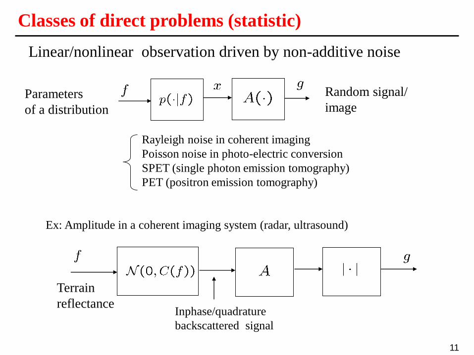
Classes of direct problems (statistic)

Rayleigh noise in coherent imaging

Poisson noise in photo-electric conversion

SPET (single photon emission tomography)

PET (positron emission tomography)

Linear/nonlinear observation driven by non-additive noise

Parameters

of a distribution

Random signal/

image

Ex: Amplitude in a coherent imaging system (radar, ultrasound)

Inphase/quadrature

backscattered signal

Terrain

reflectance

12

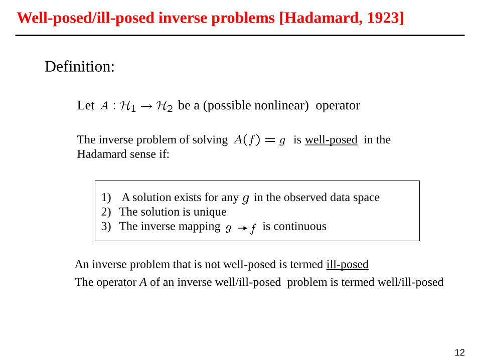
Well-posed/ill-posed inverse problems [Hadamard, 1923]

The inverse problem of solving is well-posed in the

Hadamard sense if:

1) A solution exists for any in the observed data space

2) The solution is unique

3) The inverse mapping is continuous

An inverse problem that is not well-posed is termed ill-posed

The operator A of an inverse well/ill-posed problem is termed well/ill-posed

Definition:

Let be a (possible nonlinear) operator

13

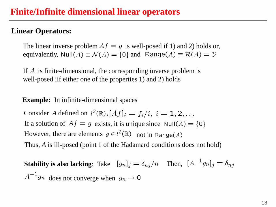
Finite/Infinite dimensional linear operators

Stability is also lacking: Take Then,

does not converge when

Consider A defined on ,

If a solution of exists, it is unique since

However, there are elements not in

Thus, A is ill-posed (point 1 of the Hadamard conditions does not hold)

Example: In infinite-dimensional spaces

The linear inverse problem is well-posed if 1) and 2) holds or,

equivalently, and

If is finite-dimensional, the corresponding inverse problem is

well-posed iif either one of the properties 1) and 2) holds

Linear Operators:

14

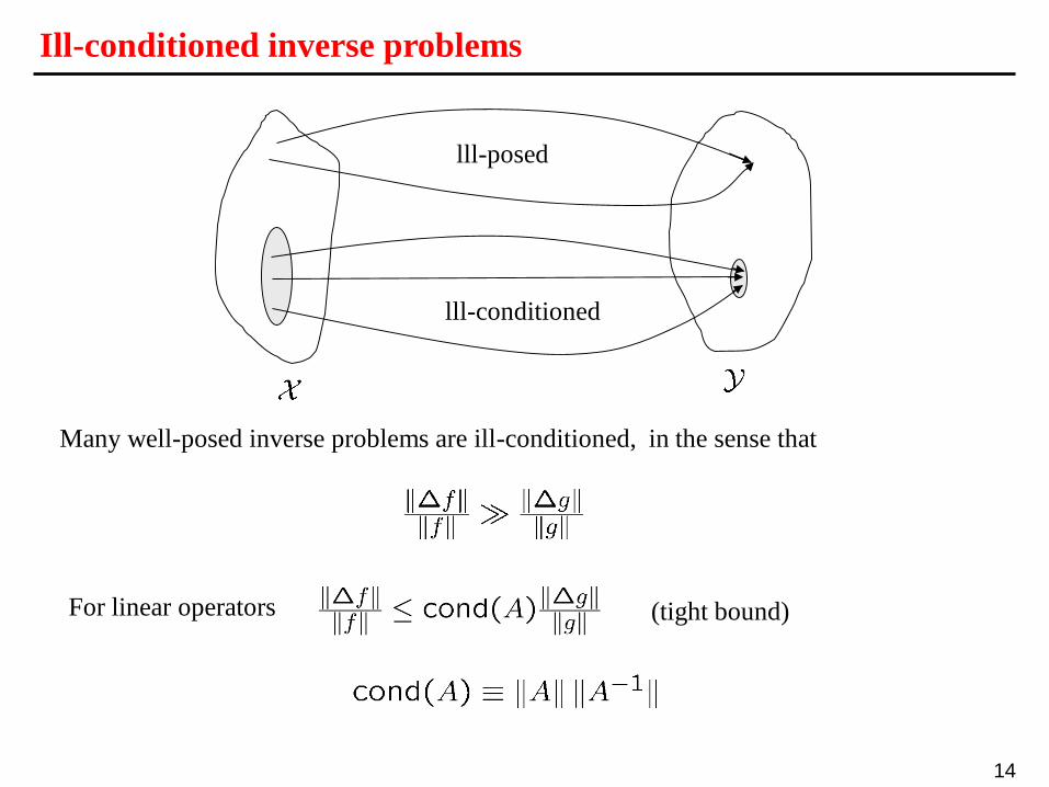
Ill-conditioned inverse problems

lll-posed

lll-conditioned

Many well-posed inverse problems are ill-conditioned, in the sense that

For linear operators (tight bound)

15

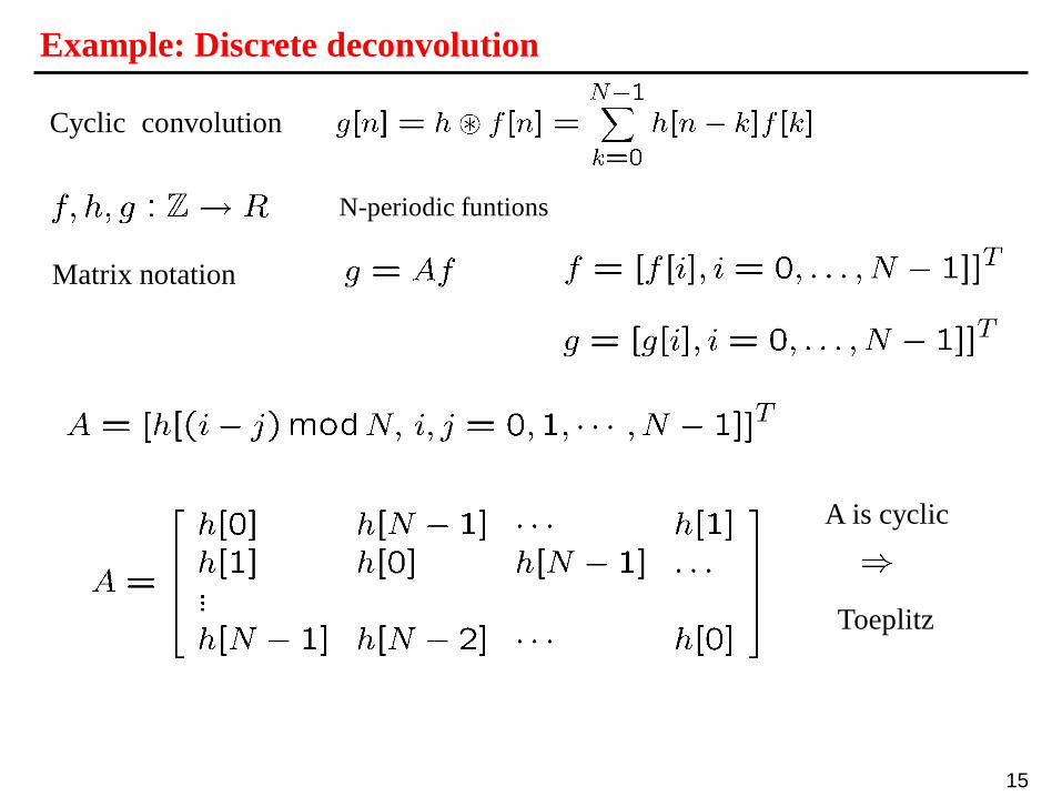
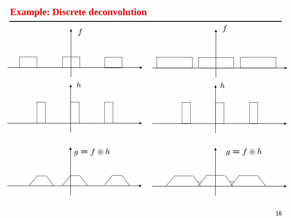
Example: Discrete deconvolution

N-periodic funtions

Cyclic convolution

Matrix notation

A is cyclic

Toeplitz

16

Example: Discrete deconvolution

17

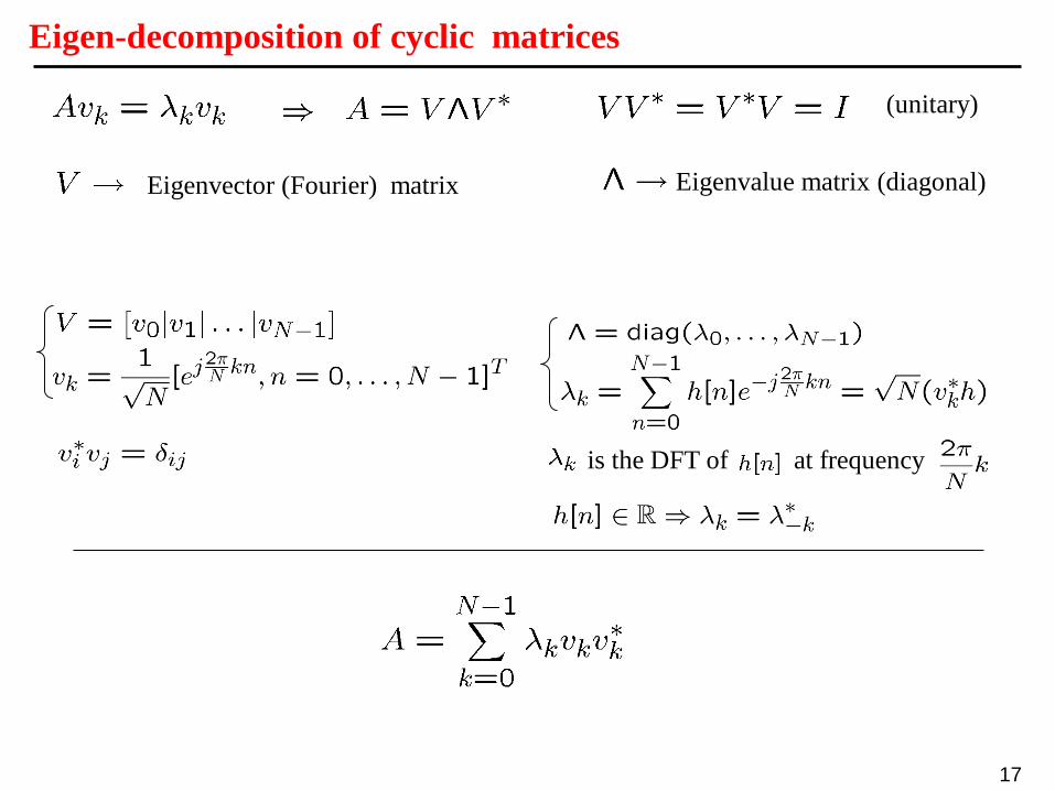
Eigen-decomposition of cyclic matrices

(unitary)

Eigenvector (Fourier) matrix Eigenvalue matrix (diagonal)

is the DFT of at frequency

18

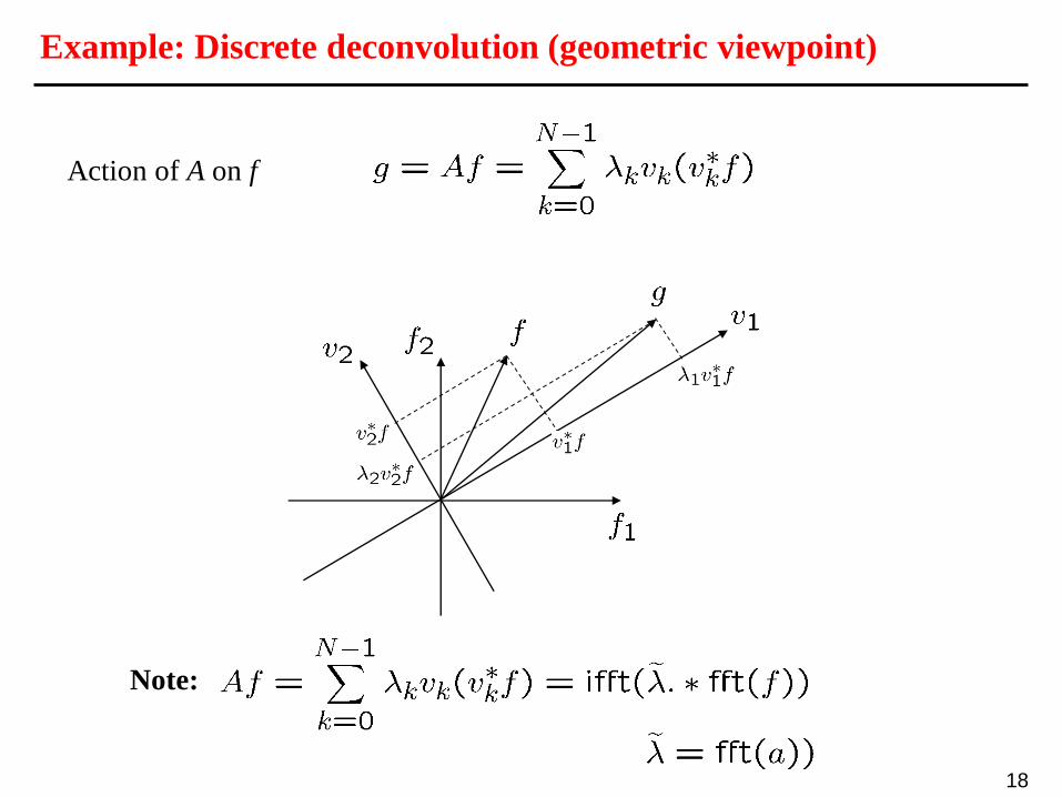
Example: Discrete deconvolution (geometric viewpoint)

Action of A on f

Note:

19

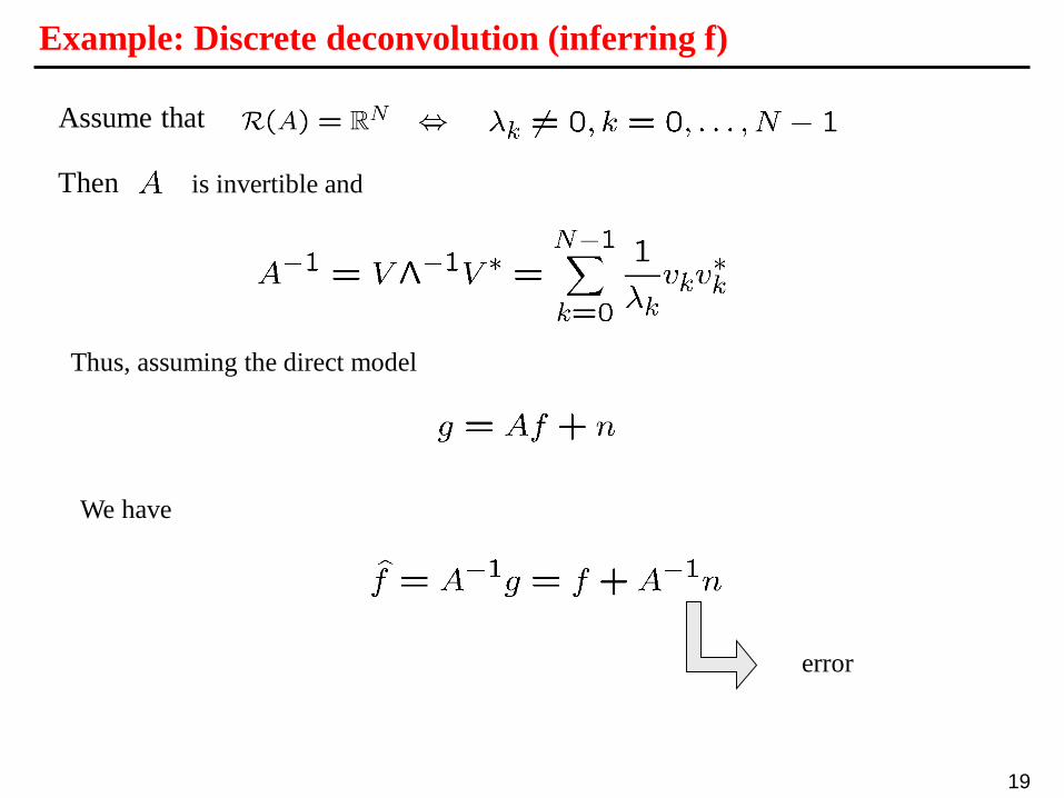
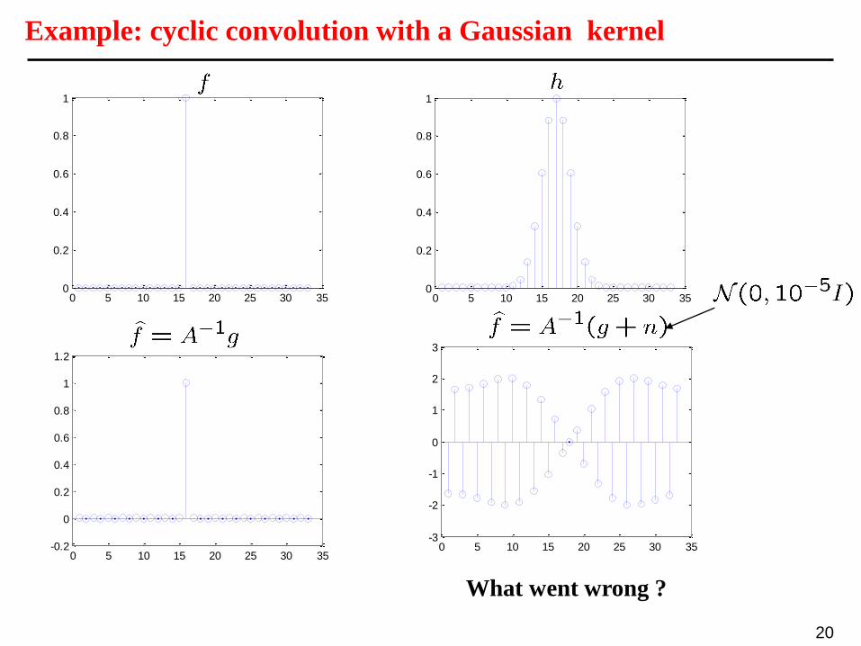
Example: Discrete deconvolution (inferring f)

Assume that

Then is invertible and

Thus, assuming the direct model

We have

error

20

Example: cyclic convolution with a Gaussian kernel

0 5 10 15 20 25 30 350

0.2

0.4

0.6

0.8

1

0 5 10 15 20 25 30 350

0.2

0.4

0.6

0.8

1

0 5 10 15 20 25 30 35-0.2

0

0.2

0.4

0.6

0.8

1

1.2

0 5 10 15 20 25 30 35-3

-2

-1

0

1

2

3

What went wrong ?

21

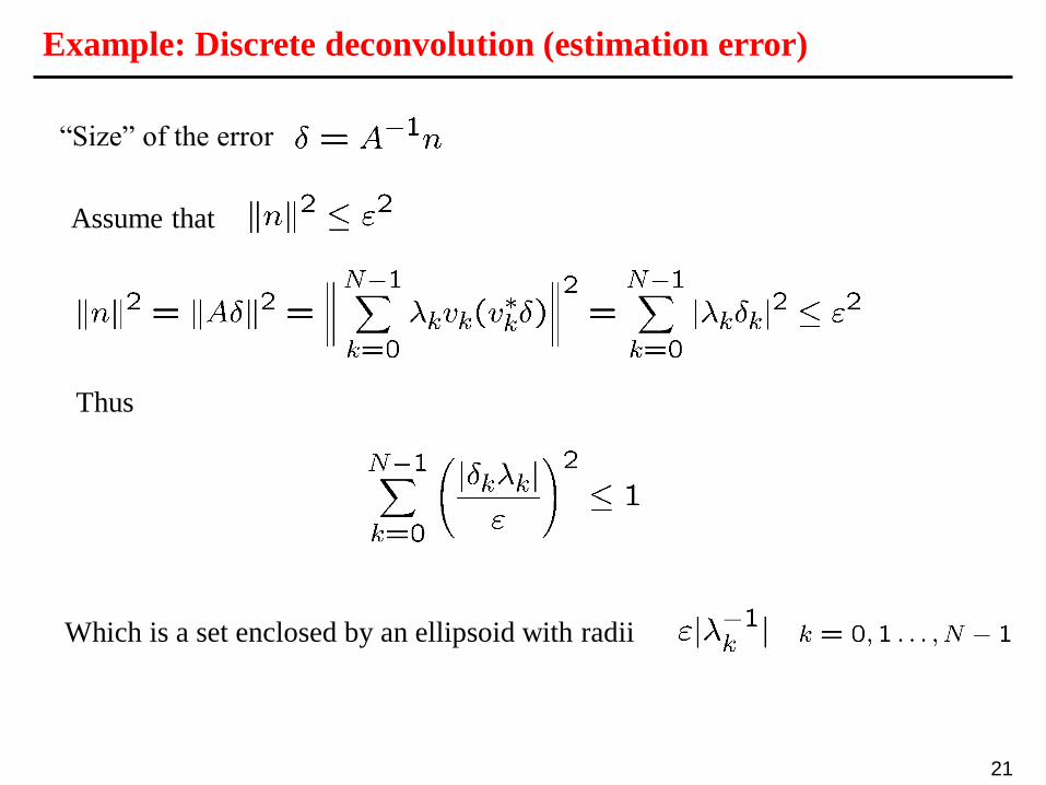
Example: Discrete deconvolution (estimation error)

“Size” of the error

Assume that

Thus

Which is a set enclosed by an ellipsoid with radii

22

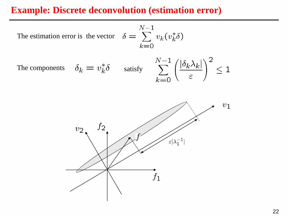
Example: Discrete deconvolution (estimation error)

The estimation error is the vector

The components satisfy

23

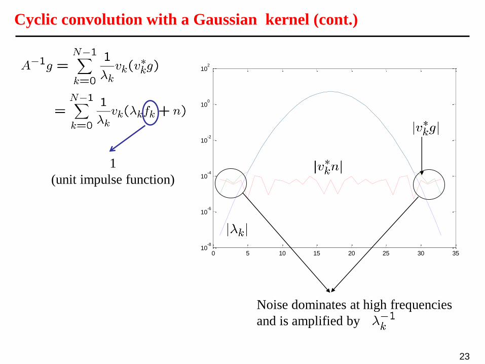
Cyclic convolution with a Gaussian kernel (cont.)

0 5 10 15 20 25 30 3510

-8

10-6

10-4

10-2

100

102

Noise dominates at high frequencies

and is amplified by

1

(unit impulse function)

24

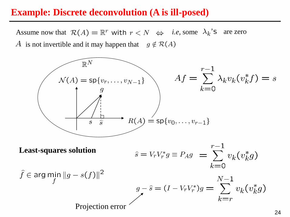
Example: Discrete deconvolution (A is ill-posed)

Assume now that

is not invertible and it may happen that

i.e, some are zero

Least-squares solution

Projection error

25

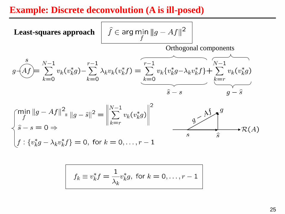
Example: Discrete deconvolution (A is ill-posed)

Least-squares approach

Orthogonal components

26

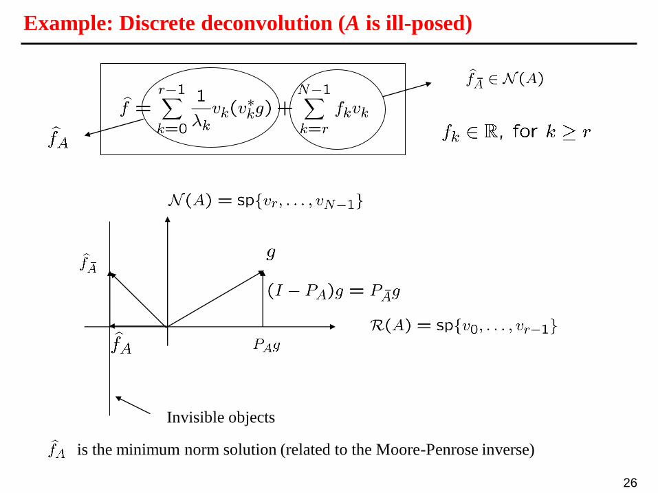
Example: Discrete deconvolution (A is ill-posed)

Invisible objects

is the minimum norm solution (related to the Moore-Penrose inverse)

27

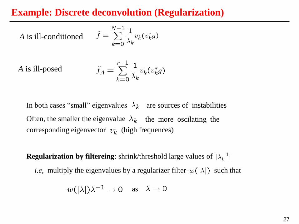
Example: Discrete deconvolution (Regularization)

A is ill-conditioned

A is ill-posed

In both cases “small” eigenvalues are sources of instabilities

Often, the smaller the eigenvalue the more oscilating the

corresponding eigenvector (high frequences)

Regularization by filtereing: shrink/threshold large values of

i.e, multiply the eigenvalues by a regularizer filter such that

as

28

Example: Discrete deconvolution

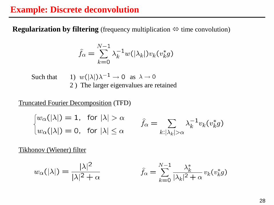
1)

2 ) The larger eigenvalues are retained

as

Regularization by filtering (frequency multiplication time convolution)

Such that

Truncated Fourier Decomposition (TFD)

Tikhonov (Wiener) filter

29

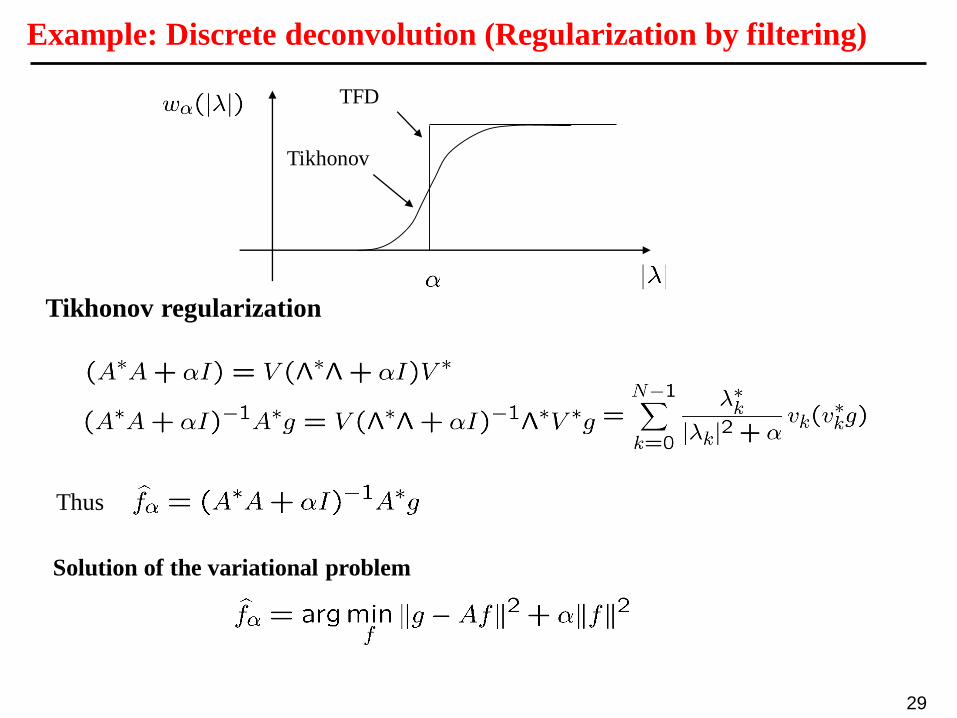
Example: Discrete deconvolution (Regularization by filtering)

TFD

Tikhonov

Tikhonov regularization

Thus

Solution of the variational problem

30

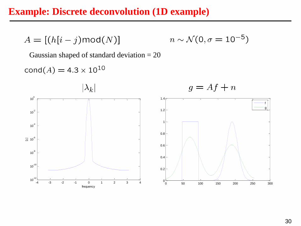
Example: Discrete deconvolution (1D example)

0 50 100 150 200 250 3000

0.2

0.4

0.6

0.8

1

1.2

1.4

f

g

Gaussian shaped of standard deviation = 20

-4 -3 -2 -1 0 1 2 3 410

-12

10-10

10-8

10-6

10-4

10-2

100

frequency

| |

31

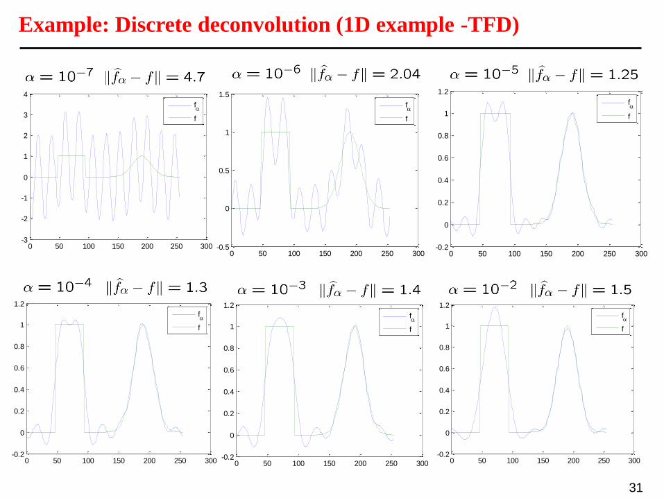
Example: Discrete deconvolution (1D example -TFD)

0 50 100 150 200 250 300-3

-2

-1

0

1

2

3

4

f

f

0 50 100 150 200 250 300-0.5

0

0.5

1

1.5

f

f

0 50 100 150 200 250 300-0.2

0

0.2

0.4

0.6

0.8

1

1.2

f

f

0 50 100 150 200 250 300-0.2

0

0.2

0.4

0.6

0.8

1

1.2

f

f

0 50 100 150 200 250 300-0.2

0

0.2

0.4

0.6

0.8

1

1.2

f

f

0 50 100 150 200 250 300-0.2

0

0.2

0.4

0.6

0.8

1

1.2

f

f

32

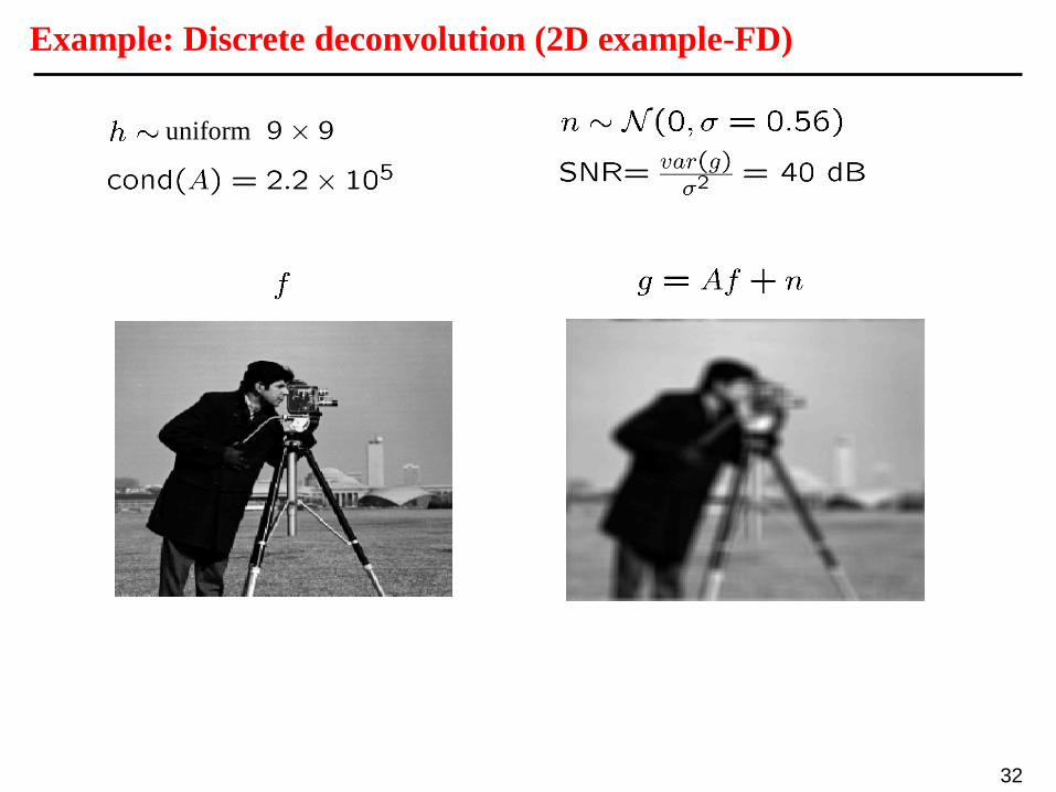
Example: Discrete deconvolution (2D example-FD)

uniform

33

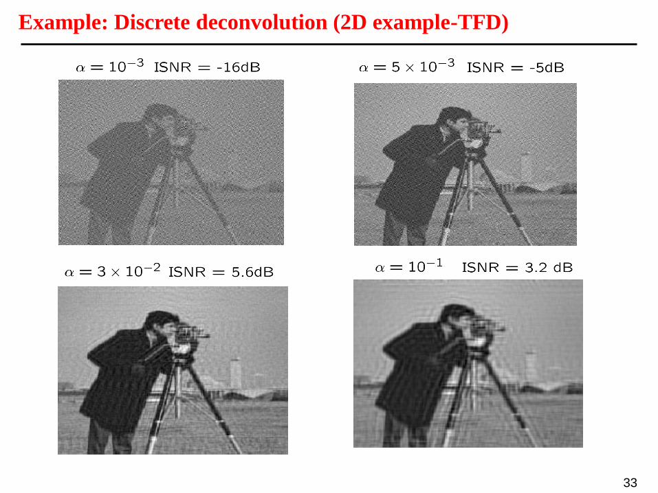
Example: Discrete deconvolution (2D example-TFD)

34

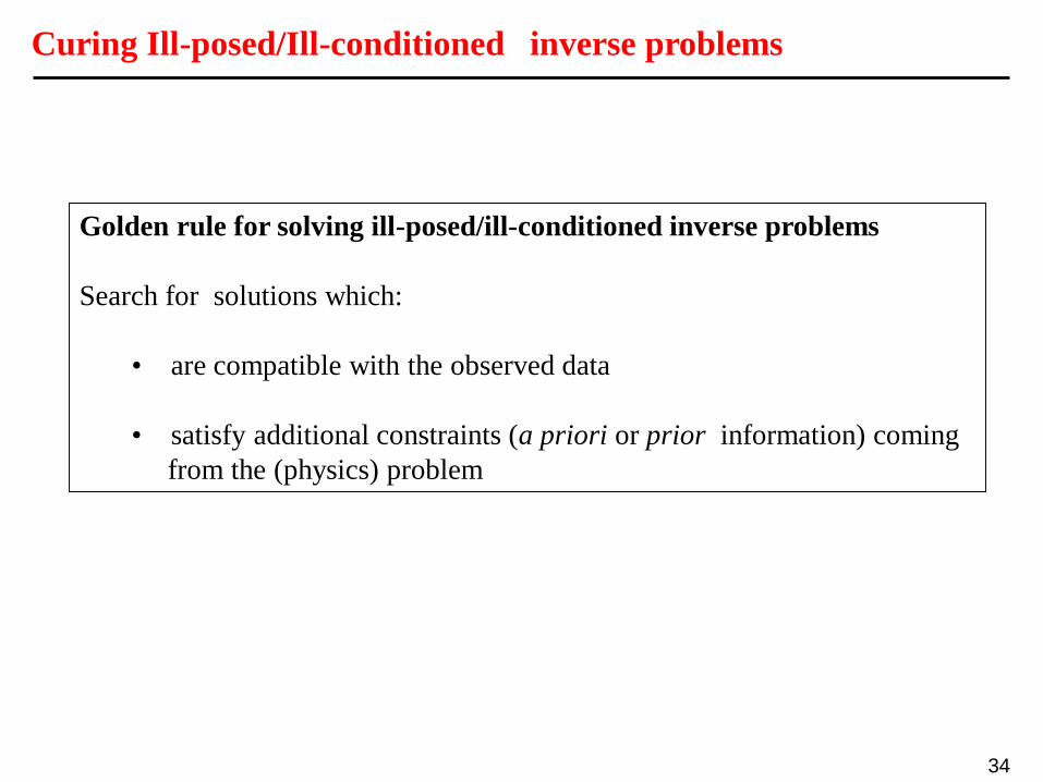
Curing Ill-posed/Ill-conditioned inverse problems

Golden rule for solving ill-posed/ill-conditioned inverse problems

Search for solutions which:

• are compatible with the observed data

• satisfy additional constraints (a priori or prior information) coming

from the (physics) problem

35

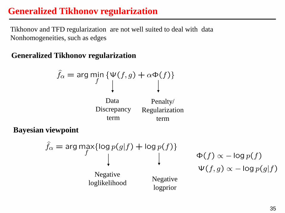
Generalized Tikhonov regularization

Tikhonov and TFD regularization are not well suited to deal with data

Nonhomogeneities, such as edges

Generalized Tikhonov regularization

Data

Discrepancy

term

Penalty/

Regularization

term

Bayesian viewpoint

Negative

loglikelihood Negative

logprior

36

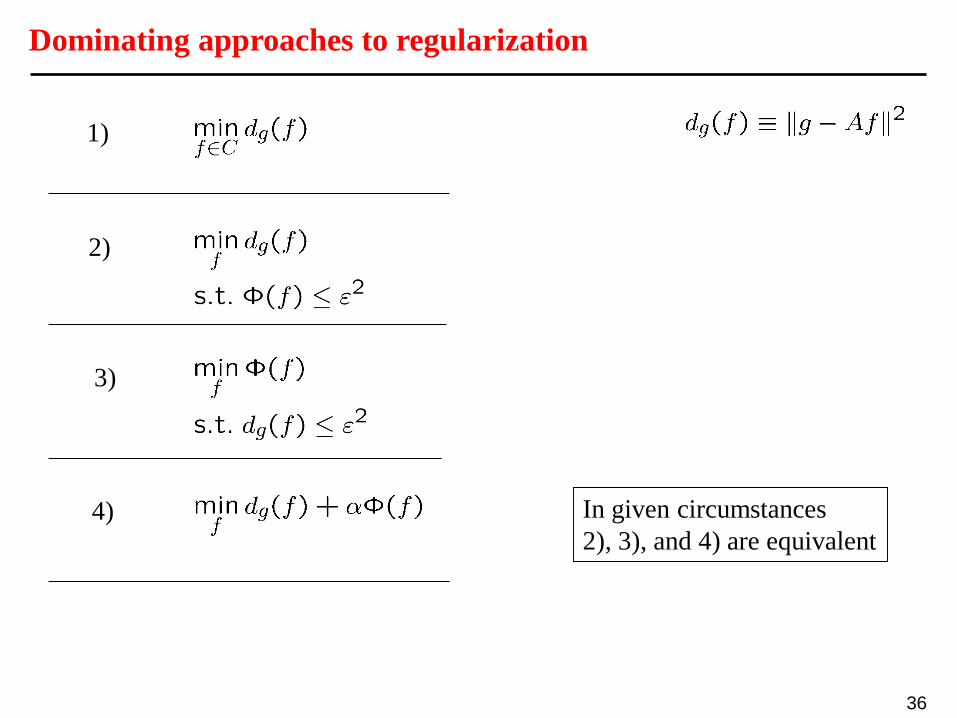
Dominating approaches to regularization

1)

2)

3)

4) In given circumstances

2), 3), and 4) are equivalent

37

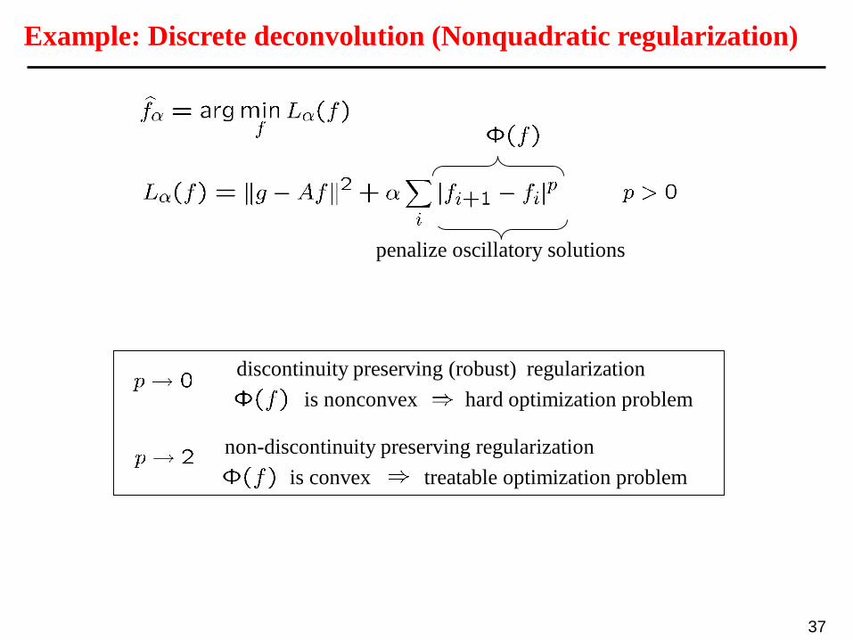
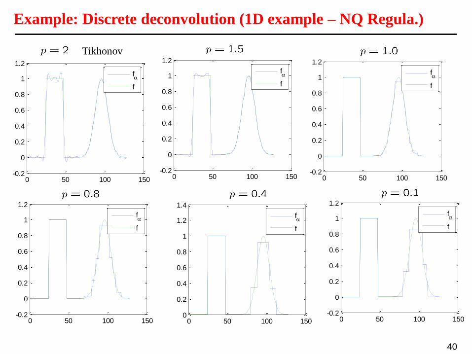
Example: Discrete deconvolution (Nonquadratic regularization)

discontinuity preserving (robust) regularization

is nonconvex hard optimization problem

non-discontinuity preserving regularization

is convex treatable optimization problem

penalize oscillatory solutions

38

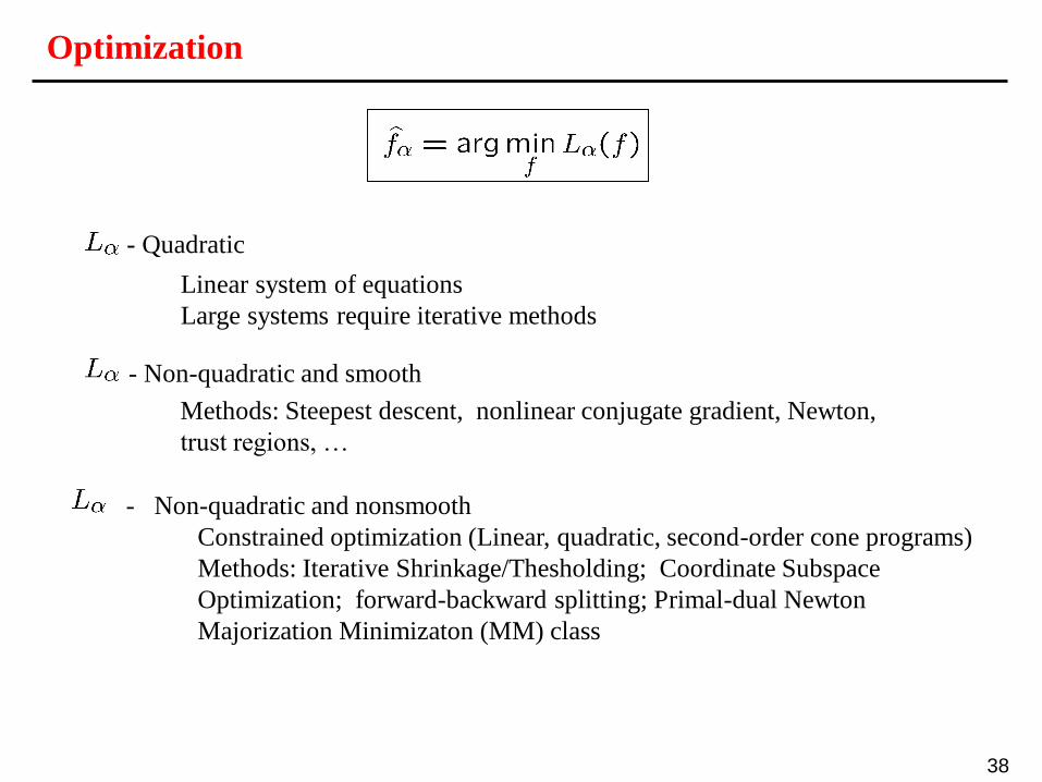
Optimization

- Quadratic

Linear system of equations

Large systems require iterative methods

- Non-quadratic and smooth

Methods: Steepest descent, nonlinear conjugate gradient, Newton,

trust regions, …

- Non-quadratic and nonsmooth

Constrained optimization (Linear, quadratic, second-order cone programs)

Methods: Iterative Shrinkage/Thesholding; Coordinate Subspace

Optimization; forward-backward splitting; Primal-dual Newton

Majorization Minimizaton (MM) class

39

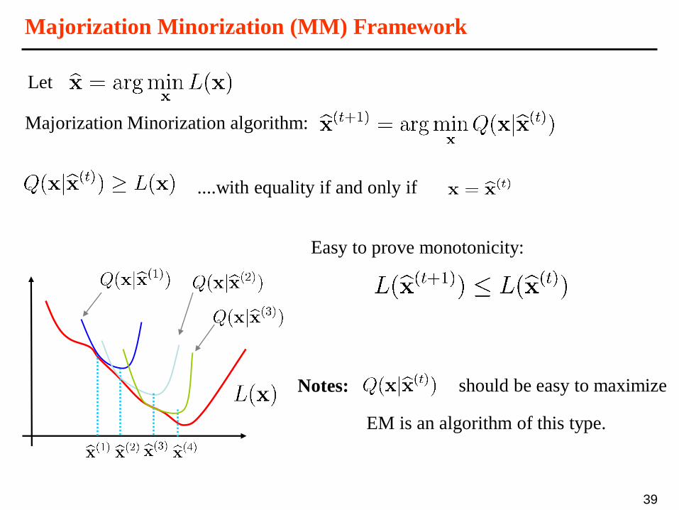
Majorization Minorization (MM) Framework

Let

Majorization Minorization algorithm:

....with equality if and only if

Easy to prove monotonicity:

Notes:

EM is an algorithm of this type.

should be easy to maximize

40

Example: Discrete deconvolution (1D example – NQ Regula.)

0 50 100 150-0.2

0

0.2

0.4

0.6

0.8

1

1.2

f

f

Tikhonov

0 50 100 150-0.2

0

0.2

0.4

0.6

0.8

1

1.2

f

f

0 50 100 150-0.2

0

0.2

0.4

0.6

0.8

1

1.2

f

f

0 50 100 150-0.2

0

0.2

0.4

0.6

0.8

1

1.2

f

f

0 50 100 1500

0.2

0.4

0.6

0.8

1

1.2

1.4

f

f

0 50 100 150-0.2

0

0.2

0.4

0.6

0.8

1

1.2

f

f

41

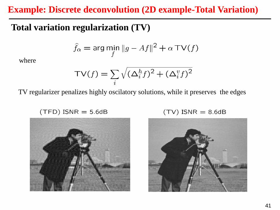
Example: Discrete deconvolution (2D example-Total Variation)

Total variation regularization (TV)

TV regularizer penalizes highly oscilatory solutions, while it preserves the edges

where

42

[Ch1. RB2, Ch1. L1]

Euclidian and Hilbert spaces of functions [App. A, RB2]

Linear operators in function spaces [App. B, RB2]

Euclidian vector spaces and matrices [App. C, RB2]

Properties of the DFT and the FFT algorithm [App. B, RB2]

Bibliography

Important topics

Matlab scripts

TFD_regularization_1D.m

TFD_regularization_2D.m

TFD_Error_1D.m

TV_regulatization_1D.m