Embed Size (px)
Citation preview
Stochastic Processes and their Applications 111 (2004) 175–206www.elsevier.com/locate/spa
Discrete-time approximation and Monte-Carlosimulation of backward stochastic di)erential
equationsBruno Boucharda ;∗, Nizar Touzib
aUniversite Paris VI, LPMA, and CREST, 4, place Jussieu, 75252 Paris, FrancebCREST and CEREMADE, Paris, France
Received 2 October 2003; accepted 6 January 2004
Abstract
We suggest a discrete-time approximation for decoupled forward–backward stochastic di)er-ential equations. The Lp norm of the error is shown to be of the order of the time step. Given asimulation-based estimator of the conditional expectation operator, we then suggest a backwardsimulation scheme, and we study the induced Lp error. This estimate is more investigated in thecontext of the Malliavin approach for the approximation of conditional expectations. Extensionsto the re:ected case are also considered.c© 2003 Elsevier B.V. All rights reserved.
MSC: 65C05; 60H07; 62G08
Keywords: Monte-Carlo methods for (re:ected) forward–backward SDEs; Malliavin calculus; Regressionestimation
1. Introduction
In this paper, we are interested in the problem of discretization and simulation ofthe (decoupled) forward–backward stochastic di)erential equation (SDE, hereafter) onthe time interval [0; 1]:
dXt = b(Xt) dt + �(Xt) dWt; −dYt = f(t; Xt ; Yt ; Zt) dt − Zt · dWt;
X0 = x and Y1 = g(X1);
∗ Corresponding author. Tel.: +33-1-44-27-3973; fax: +33-1-44-27-7223.E-mail addresses: [email protected] (B. Bouchard), [email protected] (N. Touzi).
0304-4149/$ - see front matter c© 2003 Elsevier B.V. All rights reserved.doi:10.1016/j.spa.2004.01.001

176 B. Bouchard, N. Touzi / Stochastic Processes and their Applications 111 (2004) 175–206
where W is a standard Brownian motion, b, � and f are valued, respectively, in Rn,Mn and R. The analysis of this paper extends easily to the case of re:ected backwardSDEs with z-independent generator f. This extension is presented in the last sectionof this paper.Notice that the problem of discretization and simulation of the forward components
X is well-understood (see e.g. Kloeden and Platen, 1992) and we are mainly interestedin the backward component Y . Given a partition � : 0= t0¡ · · ·¡tn=1 of the interval[0; 1], we consider the Irst naive Euler discretization of the backward SDE:
Y �ti − Y �
ti−1=−f(ti−1; X �
ti−1; Y �
ti−1; Z�
ti−1)(ti − ti−1) + Z�
ti−1· (Wti −Wti−1 )
together with the Inal data Y �tn = g(X �
tn ). The above backward equation is in fact aninInite system of equations which does not take into account the adaptability constrainton Y and Z to the Iltration. Hence, (Y �; Z�) is not uniquely deIned by the abovesystem, and is not guaranteed to be adapted.A workable backward induction scheme is obtained by taking conditional expecta-
tions. This suggests naturally the following backward procedure for the deInition ofthe discrete-time approximation (Y �; Z�):
Y �tn = g(X �
tn ); Z�ti−1
= (ti − ti−1)−1E[Y �ti (Wti −Wti−1 ) |Fti−1 ]
Y �ti−1
= E[Y �ti |Fti−1 ] + f(ti−1; X �
ti−1; Y �
ti−1; Z�
ti−1)(ti − ti−1);
for all i = 1; : : : ; n. Here {Ft} is the completed Iltration of the Brownian motion W .Our Irst main result, Theorem 3.1, is an estimate of the error Y � − Y of the orderof |�|1=2. A similar error estimate was obtained by Zhang (2001a), but with a slightlydi)erent, and less natural, discretization scheme.The key-ingredient for the simulation of the backward component Y is the following
well-known result: under standard Lipschitz conditions, the backward component andthe associated control (Y; Z), which solves the backward SDE, can be expressed as afunction of X , i.e. (Yt; Zt)=(u(t; Xt); v(t; Xt)), t6 1, for, some deterministic functions uand v. Then, the conditional expectations, involved in the above discretization scheme,reduce to the regression of Y �
ti and Y �ti (Wti −Wti−1 ) on the random variable X �
ti−1. For
instance, one can use the classical kernel regression estimation, as in CarriNere (1996),the basis projection method suggested by Longsta) and Schwartz (2001), see alsoClOement et al. (2002), or the Malliavin approach introduced in FourniOe et al. (2001),and further developed in Bouchard et al. (2004), see also Kohatsu-Higa and Pettersson(2002).Given a simulation-based approximation E�
i−1 of E[ · |Fti−1 ], we then analyse thebackward simulation scheme
Y �tn = g
(X �tn
); Z�
ti−1= (ti − ti−1)−1E�
i−1[Y�ti(Wti −Wti−1 )];
Y �ti−1
= E�i−1[Y
�ti ] + f(ti−1; X �
ti−1; Y �
ti−1; Z�
ti−1)(ti − ti−1):
Let � denote the maximum simulation error of (Ei−1 − Ei−1)[Y �ti ] and (Ei−1 − Ei−1)
[Y �ti(Wti − Wti−1 )]. Observe that � depends both on the number of simulated paths
and the time step |�|. Also, given a number N of simulated paths for the regression

B. Bouchard, N. Touzi / Stochastic Processes and their Applications 111 (2004) 175–206 177
approximation, the best estimate that one can expect for � is N−1=2, the classicalMonte-Carlo error deduced from the Central Limit Theorem. Our second main result,Theorem 4.1, states that the Lp-norm of the error due to the regression estimationis of the order |�|−1�. This rate of convergence is easily understood in the case of aregular grid, as the scheme involves |�|−1 steps, each of them requiring some regressionapproximation. As a consequence of this result, for |�|= n−1, we see that in order toachieve the rate n−1=2, one needs to use at least N=n3 simulated paths for the regressionestimation.We next investigate in more details the error (Ei−1 − Ei−1)
[Y �
ti
]and (Ei−1 −
Ei−1)[Y �
ti(Wti −Wti−1 )]. More precisely, we examine a common diQculty to the ker-
nel and the Malliavin regression estimation methods: in both methods the regressionestimator is the ratio of two statistics, which is not guaranteed to be integrable. Wesolve this diQculty by introducing a truncation procedure along the above backwardsimulation scheme. In Theorem 5.1, we show that this reduces the error to the analysisof the “integrated standard deviation” of the regression estimator. This quantity is es-timated for the Malliavin regression estimator in Section 6. The results of this sectionimply an estimate of the Lp-error Y � − Y � of the order of |�|−1−d=4pN−1=2p, whereN is the number of simulated paths for the regression estimation, see Theorem 6.2.In order to better understand this result, let � = n−1 (n time-steps), then in order toachieve an error estimate of the order n−1=2, one needs to use N = n3p+d=2 simulatedpaths for the regression estimation at each step. In the limit case p=1, this reduces toN = n3+d=2. Unfortunately, we have not been able to obtain the best expected N = n3
number of simulated paths.We conclude this introductory section by some references to the existing alternative
numerical methods for backward SDEs. First, the four step algorithm was developedby Ma et al. (1994) to solve a class of more general forward–backward SDEs (seealso Douglas et al., 1996). Their method is based on the Inite di)erence approximationof the associated PDE, which unfortunately can not be managed in high dimension.Recently, a quantization technique was suggested by Bally and PagNes (2001, 2002) forthe resolution of re:ected backward SDEs when the generator f does not depend onthe control variable z. This method is based on the approximation of the continuoustime processes on a Inite grid, and requires a further estimation of the transitionprobabilities on the grid. Discrete-time scheme based on the approximation of theBrownian motion by some discrete process have been considered in Chevance (1997),Coquet et al. (1998), Briand et al. (2001), Antonelli and Kohatsu-Higa (2000) andMa et al. (2002). This technique allows to simplify the computation of the conditionalexpectations involved at each time step. However, the implementation of these schemesin high dimension is questionable. We Inally refer to Bally (1997) for a random timescheme, which requires a further approximation of conditional expectations to give animplementation.
Notations. We shall denote by Mn;d the set of all n × d matrices with real coeQ-cients. We simply denote Rn := Mn;1 and Mn := Mn;n. We shall denote by |a| :=(∑
i; j a2i; j)1=2
the Euclydian norm on Mn;d, a∗ the transpose of a, ak the kth column

178 B. Bouchard, N. Touzi / Stochastic Processes and their Applications 111 (2004) 175–206
of a, or the kth component if a∈Rd. Finally, we denote by x ·y :=∑i xiyi the scalarproduct on Rn.
2. The simulation and discretization problem
Let (�; {F(t)}06t61; P) be a Iltered probability space equipped with a d-dimensionalstandard Brownian motion {W (t)}06t61.Consider two functions b :Rd → Rd and � : Rd → Md satisfying the Lipschitz
condition:
|b(u)− b(v)|+ |�(u)− �(v)|6K |u− v| (2.1)
for some constant K independent of u; v∈Rd. Then, it is well-known that, for anyinitial condition x∈Rd, the (forward) stochastic di)erential equation
Xt = x +∫ t
0b(Xs) ds+ �(Xs) dWs (2.2)
has a unique {Ft}-adapted solution {Xt}06t61 satisfying
E{sup06t61
|Xt |2}
¡∞:
See e.g. Karatzas and Shreve (1988). Next, let f : [0; 1] × Rd × R × Rd → R andg : Rd → R be two functions satisfying the Lipschitz condition
|g(u)− g(v)|+ |f(#)− f($)|6K(|u− v|+ |#− $|) (2.3)
for some constant K independent of u; v∈Rd and #; $∈ [0; 1]×Rd ×R×Rd. Considerthe backward stochastic di)erential equation:
Yt = g(X1) +∫ 1
tf(s; Xs; Ys; Zs) ds−
∫ 1
tZs · dWs; t6 1: (2.4)
The Lipschitz condition (2.3) ensures the existence and uniqueness of an adaptedsolution (Y; Z) to (2.4) satisfying
E
{sup06t61
|Yt |2 +∫ 1
0|Zt |2 dt
}¡∞:
See e.g. Ma and Yong (1999). Eqs. (2.2)–(2.4) deIne a decoupled system of forward–backward stochastic di)erential equations. The purpose of this paper is to study theproblem of discretization and simulation of the components (X; Y ) of the solution of(2.2)–(2.4).
Remark 2.1. Under the Lipschitz conditions (2.1)–(2.3), it is easily checked that
|Yt |6 a0 + a1|Xt |; 06 t6 1
for some parameters a0 and a1 depending on K , b(0), �(0), g(0) and f(0). In the sub-sequent paragraph, we shall derive a similar bound on the discrete-time approximation

B. Bouchard, N. Touzi / Stochastic Processes and their Applications 111 (2004) 175–206 179
of Y . The a priori knowledge of such a bound will be of crucial importance for thesimulation scheme suggested in this paper.
3. Discrete-time approximation error
In order to approximate the solution of the above BSDE, we introduce the followingdiscretized version. Let � : 0= t0¡t1¡ · · ·¡tn=1 be a partition of the time interval[0; 1] with mesh
|�| := max16i6n
|ti − ti−1|:
Throughout this paper, we shall use the notations
%�i = ti − ti−1 and %�Wi =Wti −Wti−1 ; i = 1; : : : ; n:
The forward component X will be approximated by the classical Euler scheme
X �t0 = Xt0 ;
X �ti = X �
ti−1+ b(X �
ti−1)%�
i + �(X �ti−1)%�Wi for i = 1; : : : ; n (3.1)
and we set
X �t := X �
ti−1+ b(X �
ti−1)(t − ti−1) + �(X �
ti−1)(Wt −Wti−1 ) for t ∈ (ti−1; ti):
We shall denote by {F�i }06i6n the associated discrete-time Iltration
F�i := �(X �
tj ; j6 i):
Under the Lipschitz conditions on b and �, the following Lp estimate for the errordue to the Euler scheme is well known
lim sup|�|→0
|�|−1=2 max16i6n
E
[sup06t61
|Xt − X �t |p + sup
ti−16t6ti|Xt − Xti−1 |p
]1=p¡∞ (3.2)
for all p¿ 1 (see e.g. Kloeden and Platen, 1992). We next consider the followingnatural discrete-time approximation of the backward component Y :
Y �1 = g(X �
1 );
Z�ti−1
=1%�
iE�i−1[Y
�ti %
�Wi]; (3.3)
Y �ti−1
= E�i−1[Y
�ti ] + f(ti−1; X �
ti−1; Y �
ti−1; Z�
ti−1)%�
i ; 16 i6 n; (3.4)
where E�i [ · ] = E[ · |F�
i ]. The above conditional expectations are well deIned at eachstep of the algorithm. Indeed, by a backward induction argument, it is easily checkedthat Y �
ti ∈L2 for all i.
Remark 3.1. Using an induction argument, it is easily seen that the random variablesY �ti and Z�
ti are deterministic functions of X �ti for each i = 0; : : : ; n. From the Markov

180 B. Bouchard, N. Touzi / Stochastic Processes and their Applications 111 (2004) 175–206
feature of the process X �, it then follows that the conditional expectations involved in(3.3) and (3.4) can be replaced by the corresponding regressions:
E�i−1[Y
�ti %
�Wi] = E[Y �ti %
�Wi |X �ti−1] and E�
i−1[Y�ti ] = E[Y �
ti |X �ti−1]:
For later use, we observe that the same argument shows that
Ei−1[Y �ti ] = E[Y �
ti |X �ti−1] and Ei−1[Y �
ti %�Wi] = E[Y �
ti %�Wi |X �
ti−1];
where Ei[ · ] := E[ · |Fti ] for all 06 i6 n.
Notice that (Y �; Z�) di)ers from the approximation scheme suggested in Zhang(2001b) which involves the computation of (2d + 1) conditional expectations at eachstep.For later use, we need to introduce a continuous-time approximation of (Y; Z). Since
Y �ti ∈L2 for all 16 i6 n, we deduce, from the classical martingale representation the-orem, that there exists some square integrable process Z� such that:
Y �ti+1 = E[Y �
ti+1 |Fti ] +∫ ti+1
tiZ�s · dWs
= E�i [Y
�ti+1 ] +
∫ ti+1
tiZ�s · dWs: (3.5)
We then deIne
Y �t := Y �
ti − (t − ti)f(ti; X �ti ; Y
�ti ; Z
�ti ) +
∫ t
tiZ�s · dWs; ti ¡ t6 ti+1:
The following property of the Z� is needed for the proof of the main result of thissection.
Lemma 3.1. For all 16 i6 n, we have
Z�ti−1
%�i = Ei−1
[∫ ti
ti−1
Z�s ds
]:
Proof. This is a direct consequence of the Ito isometry as by Remark 3.1
Z�ti−1
%�i = Ei−1[Y �
ti %�Wi] = Ei−1
[%�Wi
∫ ti
ti−1
Z�s · dWs
]:
We also need the following estimate proved in Theorem 3.4.3 of Zhang (2001a).
Lemma 3.2. For each 16 i6 n, de6ne
VZ�ti−1
:=1%�
iE
[∫ ti
ti−1
Zs ds |Fti−1
]:

B. Bouchard, N. Touzi / Stochastic Processes and their Applications 111 (2004) 175–206 181
Then,
lim sup|�|→0
|�|−1{max16i6n
supti−16t¡ti
E|Yt−Yti−1 |2+n∑
i=1
E
[∫ ti
ti−1
|Zt− VZ�ti−1
|2 dt]}
¡∞:
We are now ready to state our Irst result, which provides an error estimate of theapproximation scheme (3.3) and (3.4) of the same order than Zhang (2001b).
Theorem 3.1.
lim sup|�|→0
|�|−1{sup06t61
E|Y �t − Yt |2 + E
[∫ 1
0|Z�
t − Zt |2 dt]}
¡∞:
Proof. In the following, C ¿ 0 will denote a generic constant independent of i and nthat may take di)erent values from line to line. Let i∈{0; : : : ; n− 1} be Ixed, and set
(Yt := Yt − Y �t ; (Zt := Zt − Z�
t and (ft := f(t; Xt ; Yt ; Zt)− f(ti; X �ti ; Y
�ti ; Z
�ti )
for t ∈ [ti; ti+1). By Ito’s Lemma, we compute thatAt := E|(Yt |2 +
∫ ti+1
tE|(Zs|2 ds− E|(Yti+1 |2=
∫ ti+1
tE[2(Ys(fs] ds; ti6t6ti+1:
(1) Let *¿ 0 be a constant to be chosen later on. From the Lipschitz property off, together with the inequality ab6 *a2 + b2=*, this provides
At 6 E[C∫ ti+1
t|(Ys|(|�|+ |Xs − X �
ti |+ |Ys − Y �ti |+ |Zs − Z�
ti |) ds]
6∫ ti+1
t*E|(Ys|2 ds
+C*
∫ ti+1
tE[|�|2 + |Xs − X �
ti |2 + |Ys − Y �ti |2 + |Zs − Z�
ti |2] ds: (3.6)
Now observe that
E|Xs − X �ti |26C|�|; (3.7)
E|Ys − Y �ti |26 2{E|Ys − Yti |2 + E|(Yti |2}6C{|�|+ E|(Yti |2} (3.8)
by (3.2) and the estimate of Lemma 3.2. Also, with the notation of Lemma 3.2, itfollows from Lemma 3.1 that
E|Zs − Z�ti |26 2{E|Zs − VZ�
ti |2 + E|Z�ti − VZ�
ti |2}
= 2
{E|Zs − VZ�
ti |2 + E∣∣∣∣ 1%�
i+1
∫ ti+1
tiE[(Zr|Fti ] dr
∣∣∣∣2}
6 2{E|Zs − VZ�
ti |2 +1
%�i+1
∫ ti+1
tiE|(Zr|2 dr
}(3.9)

182 B. Bouchard, N. Touzi / Stochastic Processes and their Applications 111 (2004) 175–206
by Jensen’s inequality. We now plug (3.7)–(3.9) into (3.6) to obtain
At 6∫ ti+1
t*E|(Ys|2 ds+ C
*
∫ ti+1
tE[|�|+ |(Yti |2 + |Zs − VZ�
ti |2] ds
+C
*%�i+1
∫ ti+1
t
∫ ti+1
tiE|(Zr|2 dr ds (3.10)
6∫ ti+1
t*E|(Ys|2 ds+ C
*
∫ ti+1
tE[|�|+ |(Yti |2 + |Zs − VZ�
ti |2] ds
+C*
∫ ti+1
tiE|(Zr|2 dr: (3.11)
(2) From the deInition of At and (3.11), we see that, for ti6 t ¡ ti+1,
E|(Yt |26E|(Yt |2 +∫ ti+1
tE|(Zs|2 ds6 *
∫ ti+1
tE|(Ys|2 ds+ Bi; (3.12)
where
Bi := E|(Yti+1 |2+C*
{|�|2+|�|E|(Yti |2+
∫ ti+1
tiE|(Zr|2 d+
∫ ti+1
tiE|Zs − VZ�
ti |2 ds}
:
By Gronwall’s Lemma, this shows that E|(Yt |26Bie*|�| for ti6 t ¡ ti+1, which pluggedin the second inequality of (3.12) provides
E|(Yt |2 +∫ ti+1
tE|(Zs|2 ds6Bi(1 + *|�|e*|�|)6Bi(1 + C*|�|) (3.13)
for small |�|. For t= ti and * suQciently larger than C, we deduce from this inequalitythat
E|(Yti |2 +12
∫ ti+1
tiE|(Zs|2 ds
6 (1 + C|�|){E|(Yti+1 |2 + |�|2 +
∫ ti+1
tiE|Zs − VZ�
ti |2 ds}
for small |�|.(3) Iterating the last inequality, we get
E|(Yti |2 +12
∫ ti+1
tiE|(Zs|2 ds
6 (1 + C|�|)1=|�|{E|(Y1|2 + |�|+
n∑i=1
∫ ti
ti−1
E|Zs − VZ�ti−1
|2 ds}
:

B. Bouchard, N. Touzi / Stochastic Processes and their Applications 111 (2004) 175–206 183
Using the estimate of Lemma 3.2, together with the Lipschitz property of g and (3.2),this provides
E|(Yti |2 +12
∫ ti+1
tiE|(Zs|2 ds6C(1 + C|�|)1=|�|{E|(Y1|2 + C|�|}6C|�|
(3.14)
for small |�|. Summing up inequality (3.13) with t = ti, we get[1− C
*(1 + C*|�|)
] ∫ 1
0E|(Zs|2 ds
6 (1 + C*|�|)C*|�|+ (1 + C*|�|)E|(Y1|2
+[(1 + C*|�|)C
*|�| − 1
]E|(Y0|2
+[(1 + C*|�|)
(1 +
C*|�|)− 1] n−1∑
i=1
E|(Yti |2
+ (1 + C*|�|)C*
n−1∑i=0
∫ ti+1
tiE|Zs − VZti |2 ds:
For * suQciently larger than C, this proves that for small |�|:∫ 1
0E|(Zs|2 ds6C
[|�|+ E|(Y1|2 + |�|
n−1∑i=1
E|(Yti |2 +n−1∑i=0
∫ ti+1
tiE|Zs − VZti |2 ds
];
where we recall that C is a generic constant which changes from line to line. We nowuse (3.14) and the estimate of Lemma 3.2 to see that∫ 1
0E|(Zs|2 ds6C|�|:
Together with Lemma 3.2 and (3.14), this shows that Bi6C|�|, and therefore,sup06t61
E|(Yt |26C|�|
by taking the supremum over t in (3.13). This completes the proof of the theorem.
We end up this section with the following bound on the Y �ti ’s which will be used
in the simulation based approximation of the discrete-time conditional expectation op-erators E�
i , 06 i6 n− 1.
Lemma 3.3. Assume that
|g(0)|+ |f(0)|+ ‖b‖∞ + ‖�‖∞6K (3.15)

184 B. Bouchard, N. Touzi / Stochastic Processes and their Applications 111 (2004) 175–206
for some K¿ 1, and de6ne the sequence
*�n := 2K; -�
n := K;
*�i := (1− K |�|)−1{(1 + K2|�|)1=2(*�
i+1 + -�i+16K
2|�|) + 3K |�|};-�i := (1− K |�|)−1{(1 + K2|�|)1=2(1 + 2K |�|)-�
i+1 + K |�|}; 06 i6 n− 1:Then, for all 06 i6 n:
|Y �ti |6 *�
i + -�i |X �
ti |2; (3.16)
E�i−1|Y �
ti |6 {E�i−1|Y �
ti |2}1=26 *�i + -�
i [(1 + 2K |�|)|X �ti−1
|2 + 6K2|�|]; (3.17)
E�i−1|Y �
ti %�Wi|6
√|�|{*�
i + -�i [(1 + 2K |�|)|X �
ti−1|2 + 6K2|�|]}: (3.18)
Moreover,
lim sup|�|→0
max06i6n
{*�i + -�
i }¡∞:
Proof. We Irst observe that bound (3.17) is a by-product of the proof of (3.16).Bound (3.18) follows directly from (3.17) together with the Cauchy–Schwartz in-equality. In order to prove (3.16), we use a backward induction argument. First, sinceg is K-Lipschitz and g(0) is bounded by K , we have
|Y �1 |6K(1 + |X �
1 |)6K(2 + |X �1 |2) = *�
n + -�n |X �
1 |2: (3.19)
We next assume that
|Y �ti+1 |6 *�
i+1 + -�i+1|X �
ti+1 |2 (3.20)
for some Ixed 06 i6 n − 1. From the Lipschitz property of f, there exists an R ×Rd ×R×Rd-valued Fti -measurable random variable (.i; #i; /i; $i), essentially boundedby K , such that
f(ti; X �ti ; Y
�ti ; (%
�i+1)
−1E�i [Y
�ti+1%
�Wi+1])− f(0)
= .iti + #iX �ti + /iY �
ti + (%�i+1)
−1$i · E�i [Y
�ti+1%
�Wi+1]:
By the deInition of Y � in (3.4), this provides
Y �ti = E�
i [Y�ti+1 ] + %�
i+1f(0)
+%�i+1{.iti + #iX �
ti + /iY �ti + (%
�i+1)
−1$i · E�i [Y
�ti+1%
�Wi+1]}:Then, it follows from the Cauchy–Schwartz inequality and the inequality |x|6 1+ |x|2that, for |�|6 1,
(1− K |�|)|Y �ti |6 E�
i |Y �ti+1(1 + $i · %�Wi+1)|+ K |�|(2 + |X �
ti |)
6 [E�i |Y �
ti+1 |2]1=2[E�i |1 + $i · %�Wi+1|2]1=2 + K |�|(3 + |X �
ti |2):(3.21)

B. Bouchard, N. Touzi / Stochastic Processes and their Applications 111 (2004) 175–206 185
Now, since $i is Fti -measurable and bounded by K , observe that
E�i |1 + $i · %�Wi+1|26 1 + K2|�|:
We then get from (3.21):
(1− K |�|)|Y �ti |6 (1 + K2|�|)1=2[E�
i |Y �ti+1 |2]1=2 + K |�|(3 + |X �
ti |2): (3.22)
Using (3.20) and the Cauchy–Schwartz inequality, we now write that
[E�i |Y �
ti+1 |2]1=26 *�i+1 + -�
i+1{E�i (X
�ti + |�|b(X �
ti ) + �(X �ti )%
�Wi+1)4}1=2; (3.23)
where, by (3.15) and the assumption K¿ 1, direct computation leads to
{E�i (X
�ti + |�|b(X �
ti ) + �(X �ti )%
�Wi+1)4}1=26 (|X �ti |+ K |�|)2 + 3K2|�|
6 (1 + 2K |�|)|X �ti |2 + 6K2|�|: (3.24)
Together with (3.22)–(3.24), this implies that
(1− K |�|)|Y �ti |6 (1 + K2|�|)1=2{*�
i+1 + -�i+1((1 + 2K |�|)|X �
ti |2 + 6K2|�|)}+K |�|(3 + |X �
ti |2):It follows that
|Y �ti |6 *�
i + -�i |X �
ti |2:Writing -�
i in terms of � and K , we easily check that max06i6n -�i and max06i6n *�
iis uniformly bounded in |�|.
4. Error due to the regression approximation
In this section, we focus on the problem of simulating the approximation (X �; Y �)of the components (X; Y ) of the solution of the decoupled forward–backward stochas-tic di)erential equation (2.2)–(2.4). The forward component X � deIned by (3.1) canof course be simulated on the time grid deIned by the partition � by the classicalMonte-Carlo method. Then, we are reduced to the problem of simulating the approxi-mation Y � deIned in (3.3) and (3.4), given the approximation X � of X .Notice that each step of the backward induction (3.3) and (3.4) requires the com-
putation of (d + 1) conditional expectations. In practice, one can only hope to havean approximation E�
i of the conditional expectation operator E�i . Therefore, the main
idea for the deInition of an approximation of Y �, and therefore of Z�, is to replacethe conditional expectation E�
i by E�i in the backward scheme (3.3) and (3.4).
However, we would like to improve the eQciency of the approximation scheme of(Y �; Z�) when it is known to lie in some given domain. Let then ˝�={(˝�
i ; V�i )}06i6n
be a sequence of pairs of maps from Rd into R ∪ {−∞;+∞} satisfying˝�
i (X�ti )6Y �
ti 6 V �i (X�ti ) for all i = 0; : : : ; n; (4.1)
i.e. ˝�i 6 V �i are some given a priori known bounds on Y �
i for each i. For instance,one can deIne ˝� by the bounds derived in Lemma 3.3. When no bounds on Y � areknown, one may take ˝�
i =−∞ and V �i =+∞.
186 B. Bouchard, N. Touzi / Stochastic Processes and their Applications 111 (2004) 175–206
Given a random variable $ valued in R, we shall use the notation
T˝�
i ($) := ˝�i (X
�ti ) ∨ $ ∧ V �i (X
�ti );
where ∨ and ∧ denote, respectively, the binary maximum and minimum operators.Since the backward scheme (3.3) and (3.4) involves the computation of the conditionalexpectations E�
i−1[Y�ti ] and E�
i−1[Y�ti %
�Wi], we shall also need to introduce the sequencesR� = {(R�
i ; VR�i )}06i6n and I� = {(I�
i ; VI�i )}06i6n of pairs of maps from Rd into R ∪
{−∞;+∞} satisfying:R�
i−1(X�ti−1)6E�
i−1[Y�ti ]6 VR�
i−1(X�ti−1);
I�i−1(X
�ti−1)6E�
i−1[Y�ti %
�Wi]6 VI�i−1(X
�ti−1)
for all i = 1; : : : ; n. The corresponding operators TR�
i and TI�
i are deIned similarly toT˝�
i . An example of such sequences is given by Lemma 3.3.Now, given an approximation E�
i of E�i , we deIne the process (Y
�; Z�) by thebackward induction scheme:
Y �1 = Y �
1 = g(X �1 );
Z�ti−1
=1%�
iE�
i−1[Y�ti%
�Wi]; (4.2)
XY �ti−1
= E�i−1[Y
�ti ] + %�
i f(ti−1; X�ti−1
; XY �ti−1
; Z�ti−1); (4.3)
Y �ti−1
= T˝�
i−1( XY�ti−1) (4.4)
for all 16 i6 n. Recall from Remark 3.1 that the conditional expectations involvedin (3.3) and (3.4) are in fact regression functions. This simpliIes considerably theproblem of approximating E�
i .
Example 4.1 (Non-parametric regression). Let $ be an Fti+1 -measurable random vari-able, and (X �(j) ; $(j))Nj=1 be N independent copies of (X �
t1 ; : : : ; X�tn ; $). The non-parametric
kernel estimator of the regression operator E�i is deIned by
E�i [$] :=
∑Nj=1 $(j)1((hN )−1(X �(j)
ti − X �ti ))∑N
j=1 1((hN )−1(X �(j)ti − X �
ti ));
where 1 is a kernel function and hN is a bandwidth matrix converging to 0 as N → ∞.We send the reader to Bosq (1998) for details on the analysis of the error E�
i − E�i .
The above regression estimator can be improved in our context by using the a prioribounds R� and I�:
E�i−1[Y ti ] = T
R�
i−1(E�i−1[Y ti ]) and E�
i−1[Y ti%�Wi] = TI�
i−1(E�i−1[Y ti%
�Wi]):
Example 4.2 (Malliavin regression approach). Let 3 be a mapping from Rd into R,and (X �(j) )Nj=1 be N independent copies of (X �
t1 ; : : : ; X�tn ). The Malliavin regression
B. Bouchard, N. Touzi / Stochastic Processes and their Applications 111 (2004) 175–206 187
estimator of the operator E�i is deIned by
E�i [3(X
�ti+1)] :=
∑Nj=1 3(X �(j)
ti+1 )HX�ti(X �(j)
ti )S(j)∑Nj=1 HX�
ti(X �(j)
ti )S(j);
where Hx is the Heaviside function, Hx(y) =∏d
i=1 1xi6yi , and S(j) are independentcopies of some random variable S whose precise deInition is given in Section 6below. Notice that the practical implementation of this approximation procedure in thebackward induction (4.2) and (4.3) requires a slight extension of this estimator. Thisissue will be discussed precisely in Section 6.As in the previous example, the above regression estimator can be improved in our
context by using the a priori bounds R� and I�:
E�i−1[Y ti ] = T
R�
i−1(E�i−1[Y ti ]) and E�
i−1[Y ti%�Wi] = TI�
i−1(E�i−1[Y ti%
�Wi]):
Remark 4.1. The use of a priori bounds on the conditional expectation to be computedis a crucial step in our analysis. This is due to the fact that, in general, natural estimatorsE�
i , as in Examples 4.1 and 4.2, produce random variables which are not necessarilyintegrable. This integrability issue is very important in view of Theorem 4.1 below.
We now turn to the main result of this section, which provides an Lp estimate ofthe error Y � − Y � in terms of the regression errors E�
i − E�i .
Theorem 4.1. Let p¿ 1 be given, and ˝� be a sequence of pairs of maps valued inR ∪ {−∞;∞} satisfying (4.1). Then, there is a constant C ¿ 0 which only dependson (K;p) such that
‖Y �ti−Y �
ti ‖Lp6C|�| max
06j6n−1{‖(E�
j−E�j )[Y
�tj+1 ]‖Lp + ‖(E�
j − E�j )[Y
�tj+1%
�Wj+1]‖Lp}
for all 06 i6 n.
Proof. In the following, C ¿ 0 will denote a generic constant, which only depends on(K;p), that may change from line to line. Let 06 i6 n−1 be Ixed. We Irst computethat
Y �ti − XY �
ti = 6i + E�i [Y
�ti+1 − Y �
ti+1 ]
+%�i+1{f(ti; X �
ti ; Y�ti ; (%
�i+1)
−1E�i [Y
�ti+1%
�Wi+1])
−f(ti; X �ti ; XY
�ti ; (%
�i+1)
−1E�i [Y
�ti+1%
�Wi+1])}; (4.5)
where
6i := (E�i − E�
i )[Y�ti+1 ] + %�
i+1{f(ti; X �ti ; XY
�ti ; (%
�i+1)
−1E�i [Y
�ti+1%
�Wi+1])
−f(ti; X �ti ; XY
�ti ; (%
�i+1)
−1E�i [Y
�ti+1%
�Wi+1])}:From the Lipschitz property of f, we have
‖6i‖Lp 6 �i := C{‖(E�i − E�
i )[Y�ti+1 ]‖Lp + ‖(E�
i − E�i )[Y
�ti+1%
�Wi+1]‖Lp}:

188 B. Bouchard, N. Touzi / Stochastic Processes and their Applications 111 (2004) 175–206
Again, from the Lipschitz property of f, there exists an R×Rd-valued Fti -measurablerandom variable (/i; $i), essentially bounded by K , such that
f(ti; X �ti ; Y
�ti ; (%
�i+1)
−1E�i [Y
�ti+1%
�Wi+1])− f(ti; X �ti ; XY
�ti ; (%
�i+1)
−1E�i [Y
�ti+1%
�Wi+1])
=/i(Y �ti − XY �
ti) + (%�i+1)
−1$i · E�i [(Y
�ti+1 − Y �
ti+1)%�Wi+1]:
Then, it follows from (4.5) and the HYolder inequality that
(1− K |�|)|Y �ti − XY �
ti |6 |6i|+ E�i |(Y �
ti+1 − Y �ti+1)(1 + $i · %�Wi+1)|
6 |6i|+ [E�i |Y �
ti+1 − Y �ti+1 |p]1=p[E�
i |1 + $i · %�Wi+1|q]1=q
6 |6i|+ [E�i |Y �
ti+1 − Y �ti+1 |p]1=p[E�
i |1 + $i · %�Wi+1|2k ]1=2k ;where q is the conjugate of p and k¿ q=2 is an arbitrary integer. Recalling thatY �
ti = T˝�
i ( XY�ti) and Y �
ti = T˝�
i (Y�ti ), by (4.1), this provides
(1− K |�|)|Y �ti −Y �
ti |6|6i|+[E�i |Y �
ti+1−Y �ti+1 |p]1=p[E�
i |1+$i · %�Wi+1|2k ]1=2k (4.6)
by the 1-Lipschitz property of T˝�
i . Now, since $i is Fti -measurable and bounded byK , observe that
E�i |1 + $i · %�Wi+1|2k =
2k∑j=0
(2k
j
)E�i ($i · %�Wi+1)j
=k∑
j=0
(2k
2j
)E�i ($i · %�Wi+1)2j
6 1 + C|�|:We then get from (4.6):
(1− K |�|)‖Y �ti − Y �
ti‖Lp 6 ‖6i‖Lp + (1 + C|�|)1=2k‖Y �ti+1 − Y �
ti+1‖Lp
6 �i + (1 + C|�|)1=2k‖Y �ti+1 − Y �
ti+1‖Lp : (4.7)
For small |�|, it follows from this inequality that:
‖Y �ti+1 − Y �
ti+1‖Lp 61|�| (1− K |�|)−1=|�|(1 + C|�|)1=(2k|�|) max
06j6n−1�i
6C|�| max
06j6n−1�j:
Remark 4.2. In the particular case where the generator f does not depend on thecontrol variable z, Theorem 4.1 is valid for p= 1. This is easily checked by noticingthat, in this case, $i = 0 in the above proof.

B. Bouchard, N. Touzi / Stochastic Processes and their Applications 111 (2004) 175–206 189
5. Regression error estimate
In this section, we focus on the regression procedure. Let (R; S) be a pair of randomvariables. In both Examples 4.1 and 4.2, the regression estimator is based on theobservation that the regression function can be written in
r(x) := E[R|S = x] =qR(x)q1(x)
; where qR(x) := E[R6x(S)]
and 6x denotes the Dirac measure at the point x. Then, the regression estimation problemis reduced to the problem of estimating separately qR(x) and q1(x), and the maindiQculty lies in the presence of the Dirac measure inside the expectation operator.While the kernel estimator is based on approximating the Dirac measure by a kernel
function with bandwidth shrinking to zero, the Malliavin estimator is suggested by analternative representation of qR(x) obtained by integrating up the Dirac measure to theHeaviside function, see Section 6. In both cases, one deInes an estimator
rN (x; !) :=qRN (x; !)
q1N (x; !); !∈�;
where qRN (x; !) and q1N (x; !) are deIned as the means on a sample of N independent
copies {A(i)(x; !); B(i)(x; !)}16i6N of some corresponding random variables {A(x; !);B(x; !)}:
qRN (x; !) :=
1N
N∑i=1
A(i)(x; !) and q1N (x; !) :=1N
N∑i=1
B(i)(x; !):
In the Malliavin approach these random variables {A(x; !); B(x; !)} have expectationequal to {qR(x); q1(x)}, see Theorem 6.1 below. Using the above deInitions, it followsthat:
VR(x) := N Var[qRN (x)] = Var[A(x)];
V1(x) := N Var[q1N (x)] = Var[B(x)]: (5.1)
In order to prepare for the results of Section 6, we shall now concentrate on the casewhere E(A(x); B(x)) = (qR(x); q1(x)), so that (5.1) holds. A similar analysis can beperformed for the kernel approach, see Remark 5.1 below.In view of Theorem 4.1, the Lp error estimate of |Y �−Y �| is related to the Lp error
on the regression estimator. As mentioned in Remark 4.1, the regression error rN (S)−r(S) is not guaranteed to be integrable. Indeed, the classical central limit theoremindicates that the denominator q1N (x) of rN (x) has a gaussian asymptotic distribution,which induces integrability problems on the ratio qR
N (x)=q1N (x).
We solve this diQculty by introducing the a priori bounds {;(x); V;(x)} on r(x):
;(x)6 r(x)6 V;(x) for all x
and we deIne the truncated estimators
rN (x) := T;(rN (x)) := ;(x) ∨ rN (x) ∧ V;(x):
We are now ready for the main result of this section.

190 B. Bouchard, N. Touzi / Stochastic Processes and their Applications 111 (2004) 175–206
Theorem 5.1. Let R and S be random variables valued respectively in R and Rd.Assume that S has a density q1¿ 0 with respect to the Lebesgue measure on Rd.For all x∈Rd, let {A(i)(x)}16i6N and {B(i)(x)}16i6N be two families of independentand identically distributed random variables on R satisfying
E[A(i)(x)] = qR(x) and E[B(i)(x)] = q1(x) for all 16 i6N:
Set >(x) := | V;− ;|(x), and assume that
?(r; >; V1; VR) :=∫Rd
>(x)p−1[VR(x)1=2 + (|r(x)|+ >(x))V1(x)1=2] dx¡∞ (5.2)
for some p¿ 1. Then,
‖rN (S)− r(S)‖Lp 6 (2?(r; >; V1; VR)N−1=2)1=p:
Proof. We Irst estimate that
‖rN (S)− r(S)‖pLp 6 E[|rN (S)− r(S)|p ∧ >(S)p]
= E[∣∣∣∣ 6RN (S)− r(S)61N (S)
q1N (S)
∣∣∣∣p
∧ >(S)p]; (5.3)
where
6RN (x; !) := qRN (x; !)− qR(x) and 61N (x; !) := q1N (x; !)− q1(x):
For later use, we observe that
‖6RN (x)‖L16 ‖6RN (x)‖L26N−1=2VR(x)1=2;
‖61N (x)‖L16 ‖61N (x)‖L26N−1=2V1(x)1=2
by (5.1). Next, for all x∈Rd, we consider the event set
M(x) := {!∈� : |q1N (x; !)− q1(x)|6 2−1q1(x)}and observe that, for a.e. !∈�,∣∣∣∣ 6RN (x; !)− r(x)61N (x)
q1N (x; !)
∣∣∣∣p
∧ >(x)p6∣∣∣∣2 6RN (x; !)− r(x)61N (x)
q1(x)
∣∣∣∣p
∧ >(x)p1M(x)(!)
+ >(x)p1M(x)c(!): (5.4)
As for the Irst term on the right-hand side, we directly compute that for p¿ 1:∣∣∣∣2 6RN (x)− r(x)61N (x)q1(x)
∣∣∣∣p
∧ >(x)p6 2∣∣∣∣ 6RN (x)− r(x)61N (x)
q1(x)
∣∣∣∣ >(x)p−1so that
E[∣∣∣∣2 6RN (S)− r(S)61N (S)
q1(S)
∣∣∣∣p
∧ >(S)p1M(S)
]
6 2∫Rd
E|6RN (x)− r(x)61N (x)|>(x)p−1 dx
B. Bouchard, N. Touzi / Stochastic Processes and their Applications 111 (2004) 175–206 191
6 2∫Rd(‖6RN (x)‖L2 + ‖r(x)61N (x)‖L2 )>(x)p−1 dx
=2N−1=2∫Rd(VR(x)1=2 + |r(x)|V1(x)1=2)>(x)p−1 dx: (5.5)
The second term on the right-hand side of (5.4) is estimated by means of theTchebytchev inequality:
E[>(S)p1Mc(S)] = E[E(>(S)p1Mc(S) | S)]= E[>(S)pP(M(S)c | S)]= E[>(S)pP(2|q1N (S)− q1(S)|¿q1(S) | S)]6 2E[>(S)pq1(S)−1E[|q1N (S)− q1(S)| | S]]6 2E[>(S)pq1(S)−1 Var[q1N (S) | S]1=2]
= 2N−1=2∫Rd
>(x)pV1(x)1=2 dx: (5.6)
The required result follows by plugging inequalities (5.4)–(5.6) into (5.3).
Remark 5.1. Observe from the above proof, that the error estimate of Theorem 5.1could have been written in terms of ‖6RN (x)‖L1 and ‖61N (x)‖L1 instead of N−1=2VR(x)1=2
and N−1=2V1(x)1=2. In that case, the estimate of Theorem 5.1 reads
‖rN (S)− r(S)‖pLp 6 2∫Rd
>(x)p−1[‖6RN (x)‖L1 + (|r(x)|+ >(x))‖61N (x)‖L1 ] dx
a result which does not require the assumption E(A(x); B(x)) = (qR(x); q1(x)). In thekernel approach, ‖6RN (x)‖L1 and ‖61N (x)‖L1 will typically go to zero as N tends toinInity. A detailed study of the above quantity is left to future researches.
6. Malliavin calculus based regression approximation
In this section, we concentrate on the Malliavin approach for the approximation of theconditional expectation E�
i as introduced in Example 4.2. We shall assume throughoutthis section that
�(x) is invertible for all x∈Rd and b; �; �−1 ∈C∞b : (6.1)
For sake of simplicity, we shall also restrict the presentation to the case of regularsampling
%�i = ti − ti−1 = |�| for all 16 i6 n:

192 B. Bouchard, N. Touzi / Stochastic Processes and their Applications 111 (2004) 175–206
6.1. Alternative representation of conditional expectation
We start by introducing some notations. Throughout this section, we shall denote byJk the subset of Nk whose elements I = (i1; : : : ; ik) satisfy 16 i1¡ · · ·¡ik 6d. Weextend this deInition to k = 0 by setting J0 = ∅.Let I=(i1; : : : ; im) and J =(j1; : : : ; in) be two arbitrary elements in Jm and Jn. Then
{i1; : : : ; im} ∪ {j1; : : : ; jn}= {k1; : : : ; kp} for some max{n; m}6p6min{d;m+ n}, and16 k1¡ · · ·¡kp · · ·6d . We then denote I ∨ J := (k1; : : : ; kp)∈Jp.Given a matrix-valued process h, with columns denoted by hi, and a random variable
F , we denote
Shi [F] :=
∫ ∞
0Fhi
t · dWt for i = 1; : : : ; k; and ShI [F] := Sh
i1 ◦ · · · ◦ Shik [F]
for I=(i1; : : : ; ik)∈Jk , whenever these stochastic integrals exist in the Skorohod sense.We extend this deInition to k =0 by setting Sh
∅[F] := F . Similarly, for I ∈Jk , we set
Sh−I [F] := Sh
VI [F];
where VI ∈Jd−k and I ∨ VI is the unique element of Jd.Let ’ be a C0b (Rd
+), i.e. continuous and bounded, mapping from Rd+ into R. We say
that ’ is a smooth localizing function if
’(0) = 1 and @I’∈C0b (Rd+) for all k = 0; : : : ; d and I ∈Jk :
Here, @I’= @k’=@xi1 : : : @xik . For k = 0, Jk = ∅, and we set @∅’ := ’. We denote byL the collection of all smooth localization functions.With these notations, we introduce the set H(X �
ti ) (16 i6 n− 1) as the collectionof all matrix-valued L2(F1) processes h satisfying∫ ∞
0DtX �
ti ht dt = Id and∫ ∞
0DtX �
ti+1ht dt = 0 (6.2)
(here Id denotes the identity matrix of Md) and such that, for any aQne functiona : Rd → R,
ShI [a(%
�Wi+1)’(X �ti )] is well-deIned in D1;2
for all I ∈Jk ; k6d and ’∈L: (6.3)
For later use, we observe that by a straightforward extension of Remark 3.4 inBouchard et al. (2004), we have the representation:
Shi [a(%�Wi+1)’(X �ti − x)] =
d∑j=0
(−1)j∑J∈Jj
@J’(X �ti − x)Shi
−J [a(%�Wi+1)] (6.4)
for any aQne function a : Rd → R.
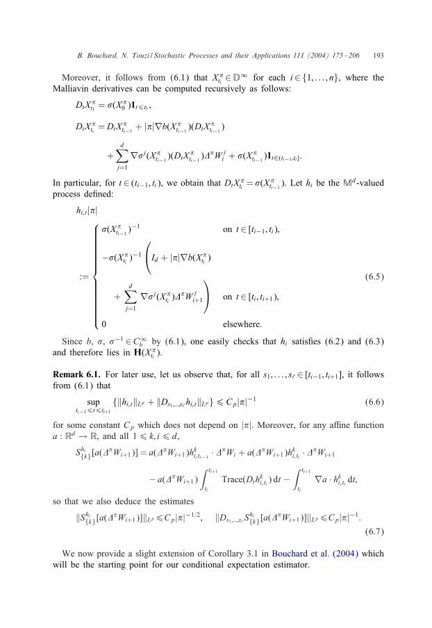
B. Bouchard, N. Touzi / Stochastic Processes and their Applications 111 (2004) 175–206 193
Moreover, it follows from (6.1) that X �ti ∈D∞ for each i∈{1; : : : ; n}, where the
Malliavin derivatives can be computed recursively as follows:
DtX �t1 = �(X �
0 )1t6t1 ;
DtX �ti =DtX �
ti−1+ |�|∇b(X �
ti−1)(DtX �
ti−1)
+d∑
j=1
∇�j(X �ti−1)(DtX �
ti−1)%�Wj
i + �(X �ti−1)1t∈(ti−1 ;ti]:
In particular, for t ∈ (ti−1; ti), we obtain that DtX �ti = �(X �
ti−1). Let hi be the Md-valued
process deIned:
hi; t |�|
:=
�(X �ti−1)−1 on t ∈ [ti−1; ti);
−�(X �ti )
−1
Id + |�|∇b(X �
ti )
+d∑
j=1
∇�j(X �ti )%
�Wji+1
on t ∈ [ti; ti+1);
0 elsewhere:
(6.5)
Since b, �, �−1 ∈C∞b by (6.1), one easily checks that hi satisIes (6.2) and (6.3)
and therefore lies in H(X �ti ).
Remark 6.1. For later use, let us observe that, for all s1; : : : ; s‘ ∈ [ti−1; ti+1], it followsfrom (6.1) that
supti−16t6ti+1
{‖hi; t‖Lp + ‖Ds1 ;:::;s‘hi; t‖Lp}6Cp|�|−1 (6.6)
for some constant Cp which does not depend on |�|. Moreover, for any aQne functiona : Rd → R, and all 16 k; i6d,
Shi{k}[a(%
�Wi+1)] = a(%�Wi+1)hki; ti−1
· %�Wi + a(%�Wi+1)hki; ti · %�Wi+1
− a(%�Wi+1)∫ ti+1
tiTrace(Dthk
i; ti) dt −∫ ti+1
ti∇a · hk
i; ti dt;
so that we also deduce the estimates
‖Shi{k}[a(%
�Wi+1)]‖Lp6Cp|�|−1=2; ‖Ds1 ;:::;s‘Shi{k}[a(%
�Wi+1)]‖Lp6Cp|�|−1:(6.7)
We now provide a slight extension of Corollary 3.1 in Bouchard et al. (2004) whichwill be the starting point for our conditional expectation estimator.

194 B. Bouchard, N. Touzi / Stochastic Processes and their Applications 111 (2004) 175–206
Theorem 6.1. Let % be a real-valued mapping and # be a (vector) random variableindependent of �(X �
ti ; 16 i6 n) with R := %(X �ti+1 ; #)a(%
�Wi+1)∈L2, for some a<nefunction a : Rd → R. Then, for all localizing functions ’, ∈L:
E[R |X �ti = x] =
E[QR[hi; ’](x)]E[Q1[hi; ](x)]
; (6.8)
where
QR[hi; ’](x) := Hx(X �ti )%(X
�ti+1 ; #)S
hi [a(%�Wi+1)’(X �ti − x)]
and Shi = Shi(1; :::;d). Moreover, if q�
i denotes the density of X �ti , then,
q�i (x) = E[Q1[hi; ’](x)];
where Q1 is de6ned as QR by replacing R by 1.
Remark 6.2. The above theorem holds for any random variable F ∈D∞, instead ofthe particular aQne transformation of the Brownian increments a(%�Wi+1). One onlyhas to change the deInition of the set of localizing functions L accordingly in orderto ensure that the involved Skorohod integrals are well deIned. However, we shallsee in Section 4.2 that we only need this characterization for the aQne functionsak(x)=1k=0+xk1k¿1, 06 k6d. Indeed, writing Y �
ti+1 as %(X�ti+1 ; $), we are interested in
computing E�i [Y
�ti+1 ]=E�
i [Y�ti+1a0(%
�Wi+1)] and E�i [Y
�ti+1%
�Wki+1]=E�
i [Y�ti+1ak(%�Wi+1)],
16 k6d, see also the deInition of Ri after (6.12).
6.2. Application to the estimation of E�
The algorithm is inspired from the work of CarriNere (1996), Longsta) andSchwartz (2001)and Lions and Regnier (2001). We consider nN copies (X �(1); : : : ; X �(nN ) )of the discrete-time process X � on the grid �, where N is some positive integer. Set
Ni := {(i − 1)N + 1; : : : ; iN}; 16 i6 n:
For ease of notation, we write X �(0) for X �. We consider the approximation scheme(4.2)–(4.4) with an approximation of conditional expectation operator E�
i suggested byTheorem 6.1. At each time step ti of this algorithm, we shall make use of the subsetXi := (X �(j) ; j∈Ni). The independence of the Xi’s is crucial as explained in Remark6.3 below.Initialization: For j∈{0} ∪Nn, we set
Y �(j)1 := Y �(j)
1 = g(X �(j)1 ): (6.9)
Backward induction: For i = n; : : : ; 2, we set, for j∈{0} ∪Ni−1:
Z�(j)ti−1
=1|�| E
�(j)i−1[Y
�(j)ti %�W ( j)
i ]; (6.10)
XY �(j)ti−1
= E�(j)i−1[Y
�(j)ti ] + |�|f(ti−1; X �(j)
ti−1; XY �(j)
ti−1; Z�(j)
ti−1);
Y �(j)ti−1
:= T˝�(j)
i−1 ( XY�(j)ti−1); (6.11)
B. Bouchard, N. Touzi / Stochastic Processes and their Applications 111 (2004) 175–206 195
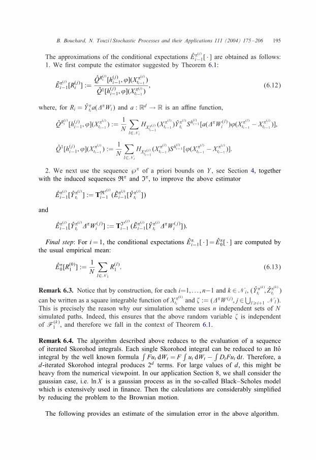
The approximations of the conditional expectations E�(j)i−1[ · ] are obtained as follows:
1. We Irst compute the estimator suggested by Theorem 6.1:
E�(j)i−1[R
(j)i ] :=
QR(j)i [h(j)i−1; ’](X�(j)ti−1)
Q1[h(j)i−1; ’](X�(j)ti−1)
; (6.12)
where, for Ri = Y �ti a(%
�Wi) and a : Rd → R is an aQne function,
QR(j)i [h(j)i−1; ’](X�(j)ti−1) :=
1N
∑l∈Ni
HX �(j)ti−1
(X �(l)ti−1)Y �(l)
ti Sh(l)i−1 [a(%�W (l)i )’(X �(l)
ti−1− X �(j)
ti−1)];
Q1[h(j)i−1; ’](X�(j)ti−1) :=
1N
∑l∈Ni
HX �(j)ti−1
(X �(l)ti−1)Sh(l)i−1 [’(X �(l)
ti−1− X �(j)
ti−1)]:
2. We next use the sequence ˝� of a priori bounds on Y , see Section 4, togetherwith the induced sequences R� and I�, to improve the above estimator
E�(j)i−1[Y
�(j)ti ] := TR�(j)
i−1 (E�(j)i−1[Y
�(j)ti ])
and
E�(j)i−1[Y
�(j)ti %�W ( j)
i ] := TI�(j)
i−1 (E�(j)i−1[Y
�(j)ti %�W ( j)
i ]):
Final step: For i=1, the conditional expectations E�i−1[ · ] = E�
0[ · ] are computed bythe usual empirical mean:
E�0[R
(0)1 ] :=
1N
∑l∈N1
R(l)1 : (6.13)
Remark 6.3. Notice that by construction, for each i=1; : : : ; n−1 and k ∈Ni, (Y �(k)ti ; Z�(k)
ti )
can be written as a square integrable function of X �(k)ti and $ := (%�W (j); j∈⋃l¿i+1 Nl).
This is precisely the reason why our simulation scheme uses n independent sets of Nsimulated paths. Indeed, this ensures that the above random variable $ is independentof F(k)
1 , and therefore we fall in the context of Theorem 6.1.
Remark 6.4. The algorithm described above reduces to the evaluation of a sequenceof iterated Skorohod integrals. Each single Skorohod integral can be reduced to an Itointegral by the well known formula
∫Fut dWt = F
∫ut dWt −
∫DtFut dt. Therefore, a
d-iterated Skorohod integral produces 2d terms. For large values of d, this might beheavy from the numerical viewpoint. In our application Section 8, we shall consider thegaussian case, i.e. ln X is a gaussian process as in the so-called Black–Scholes modelwhich is extensively used in Inance. Then the calculations are considerably simpliIedby reducing the problem to the Brownian motion.
The following provides an estimate of the simulation error in the above algorithm.

196 B. Bouchard, N. Touzi / Stochastic Processes and their Applications 111 (2004) 175–206
Theorem 6.2. Let p¿ 1 and ’∈L satisfyingd∑
k=0
∑I∈Jk
∫Rd
|u|4p+2 @I’(u)2 du¡∞:
Consider the function ’�(x) =’(|�|−1=2x) as a localizing function in (4.2)–(4.4) and(6.12). Let ˝�, R�, I� be the bounds de6ned by Lemma 3.3. Then,
lim sup|�|→0
max06i6n
|�|p+d=4N 1=2‖Y �ti − Y �
ti ‖pLp ¡∞:
The above estimate is obtained in two steps. First, Theorem 4.1 reduces the problemto the analysis of the regression simulation error. Next, for 16 i6 n, the result followsfrom Theorem 6.3 which is the main object of the subsequent paragraph. The case i=0is trivial as the regression estimator (6.13) is the classical empirical mean.
Remark 6.5. In the particular case where the generator f does not depend on thecontrol variable z, the above proposition is valid with p=1. This follows from Remark4.2.
Remark 6.6. In the previous proposition, we have introduced the normalized localizingfunction ’�(x) = ’(|�|−1=2x). This normalization is necessary for the control of theerror estimate as |�| tends to zero. An interesting observation is that, in the casewhere R is of the form %(X �
ti+1 ; $)a(%�Wi+1) for some aQne function a : Rd → R,
this normalization is in agreement with Bouchard et al. (2004) who showed that theminimal integrated variance within the class of separable localization functions is givenby ’(x) = exp(−� · x) with
(�i)2 =E[{R∑d−1
k=0 (−1)k∑
i ∈I∈JkSh−I [a(%
�Wi+1)]∏
j∈I �j}2]E[{R∑d−1
k=0 (−1)k∑
i ∈I∈JkSh−(I∨i)[a(%
�Wi+1)]∏
j∈I �j}2]; 16 i6d:
Indeed, we will show in Lemma 6.1 below that ShI [a(%
�Wi+1)] is of order |�|−|I |=2,and therefore the above ratio is of order |�|−1.
6.3. Analysis of the regression error
According to Theorem 6.1, the Lp estimate of the regression error depends on theintegrated standard deviation ? deIned in (5.2). In order to analyse this term, westart by
Lemma 6.1. For any integer m=0; : : : ; d, I ∈Jm, and any a<ne function a : Rd → R,we have
lim sup|�|→0
|�|m=2 max16i6n−1
‖ShiI [a(%
�Wi+1)]‖Lp ¡∞
for all p¿ 1.

B. Bouchard, N. Touzi / Stochastic Processes and their Applications 111 (2004) 175–206 197
Proof. Let d¿ j1¿ · · ·¿jm¿ 1 be m integers, and deIne Ik := (jm−k ; : : : ; j1). Forease of presentation, we introduce the process hi := |�|hi, and we observe thatShiI = |�|−mShi
I , by linearity of the Skorohod integral. We shall also write ShiI for
ShiI [a(%
�Wi+1)]. In order to prove the required result, we intend to show that
for all integers 06 ‘6 k6m− 1 and all . := (s1; : : : ; s‘)∈ [ti−1; ti+1]‘;
‖D.ShiIk ‖Lp 6Cp|�|(k−‘)=2; (6.14)
where Cp is a constant which does not depend on �, and .=∅, D.F=F , whenever ‘=0.We shall use a backward induction argument on the variable k. First, for k = m − 1,(6.14) follows from (6.7). We next assume that (6.14) holds for some 16 k6m− 1,and we intend to extend it to k−1. We Irst need to introduce some notations. Let S‘
be the collection of all permutations � of the set (1; : : : ; ‘). For �∈S‘ and some integeru6 ‘, we set .�u := (s�(1); : : : ; s�(u)) and V.�u := (s�(u+1); : : : ; s�(‘)), with the convention.�0 = V.�‘ = ∅.Let ‘6 k − 1 be Ixed. By direct computation, we see that
‖D.ShiIk−1
‖Lp 6∑�∈S‘
‘∑u=0
‖D.�u ShiIk ‖L2p‖D V.�u S
hijm−k+1
‖L2p
+∫ ti+1
ti−1
‖D.�uDtShiIk ‖L2p‖D V.�u h
jm−k+1t ‖L2p dt
by Cauchy–Schwarz inequality. By (6.7) and the induction hypothesis (6.14), thisprovides
‖D.ShiIk+1‖Lp 6C
∑�∈S‘
(|�|(k−‘)=2|�|1=2 +
‘−1∑u=0
|�|(k−u)=2 + |�|‘∑
u=0
|�|(k−u−1)=2)
6C∑�∈S‘
(|�|(k+1−‘)=2 +
‘−1∑u=0
|�|(k+1−‘)=2 +‘∑
u=0
|�|(k+1−‘)=2
)
= C|�|(k+1−‘)=2;
where C is a generic constant, independent of |�| and i, with di)erent values from lineto line.
Lemma 6.2. Let L be a map from Rd into R with polynomial growth
supx∈Rd
|L(x)|1 + |x|m ¡∞ for some m¿ 1:
Let ’∈L be such thatd∑
k=0
∑I∈Jk
∫Rd
|u|m@I’(u)2 du¡∞:
198 B. Bouchard, N. Touzi / Stochastic Processes and their Applications 111 (2004) 175–206
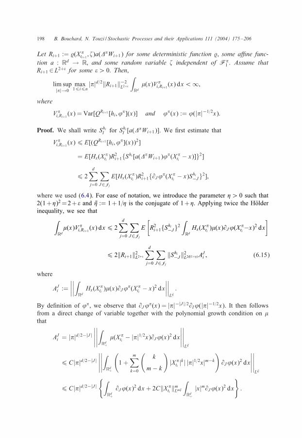
Let Ri+1 := %(X �ti+1 ; $)a(%
�Wi+1) for some deterministic function %, some a<ne func-tion a : Rd → R, and some random variable $ independent of F�
1 . Assume thatRi+1 ∈L2+6 for some 6¿ 0. Then,
lim sup|�|→0
max16i6n
|�|d=2‖Ri+1‖−2L2+6
∫Rd
L(x)V�i;Ri+1
(x) dx¡∞;
where
V�i;Ri+1
(x) = Var[QRi+1 [hi; ’�](x)] and ’�(x) := ’(|�|−1=2x):
Proof. We shall write ShiI for Shi
I [a(%�Wi+1)]. We Irst estimate that
V�i;Ri+1
(x)6 E[(QRi+1 [hi; ’�](x))2]
= E[Hx(X �ti )R
2i+1{Shi [a(%�Wi+1)’�(X �
ti − x)]}2]
6 2d∑
j=0
∑J∈Jj
E[Hx(X �ti )R
2i+1{@J’�(X �
ti − x)Shi−J}2];
where we used (6.4). For ease of notation, we introduce the parameter �¿ 0 such that2(1+�)2 =2+ 6 and V� := 1+1=� is the conjugate of 1+�. Applying twice the HYolderinequality, we see that∫
RdL(x)V�
i;Ri+1(x) dx6 2
d∑j=0
∑J∈Jj
E[R2i+1{Shi
−J}2∫Rd
Hx(X �ti )L(x)@J’(X �
ti −x)2 dx]
6 2‖Ri+1‖2L2+6
d∑j=0
∑J∈Jj
‖Shi−J‖2L2 V�(1+�)AJ
i ; (6.15)
where
AJi :=
∣∣∣∣∣∣∣∣∫Rd
Hx(X �ti )L(x)@J’�(X �
ti − x)2 dx∣∣∣∣∣∣∣∣L V�
:
By deInition of ’�, we observe that @J’�(x) = |�|−|J |=2@I’(|�|−1=2x). It then followsfrom a direct change of variable together with the polynomial growth condition on Lthat
AJi = |�|d=2−|J |
∣∣∣∣∣∣∣∣∣∣∫Rd+
L(X �ti − |�|1=2x)@J’(x)2 dx
∣∣∣∣∣∣∣∣∣∣L V�
6C|�|d=2−|J |∣∣∣∣∣∣∣∣∣∣∫Rd+
(1 +
m∑k=0
(k
m− k
)|X �
ti |k | |�|1=2x|m−k
)@J’(x)2 dx
∣∣∣∣∣∣∣∣∣∣L V�
6C|�|d=2−|J |{∫
Rd+
@J’(x)2 dx + 2C‖X �ti ‖mLm V�
∫Rd+
|x|m@J’(x)2 dx
}:
B. Bouchard, N. Touzi / Stochastic Processes and their Applications 111 (2004) 175–206 199
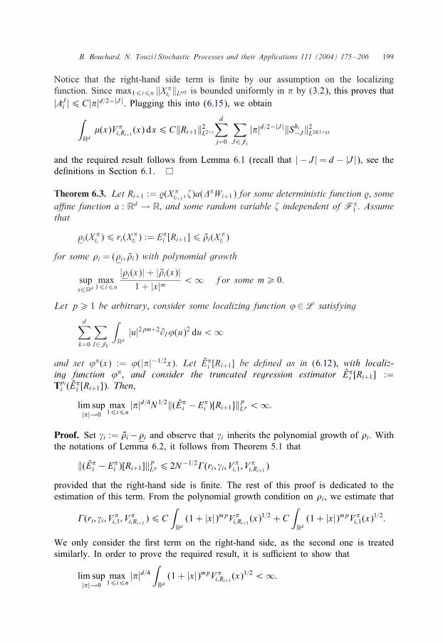
Notice that the right-hand side term is Inite by our assumption on the localizingfunction. Since max16i6n ‖X �
ti ‖Lm V� is bounded uniformly in � by (3.2), this proves that|AJ
i |6C|�|d=2−|J |. Plugging this into (6.15), we obtain∫Rd
L(x)V�i;Ri+1
(x) dx6C‖Ri+1‖2L2+6
d∑j=0
∑J∈Jj
|�|d=2−|J |‖Shi−J‖2L2 V�(1+�)
and the required result follows from Lemma 6.1 (recall that | − J |= d− |J |), see thedeInitions in Section 6.1.
Theorem 6.3. Let Ri+1 := %(X �ti+1 ; $)a(%
�Wi+1) for some deterministic function %, somea<ne function a : Rd → R, and some random variable $ independent of F�
1 . Assumethat
;i(X �ti )6 ri(X �
ti ) := E�i [Ri+1]6 V;i(X �
ti )
for some ;i = (;i; V;i) with polynomial growth
supx∈Rd
max16i6n
|;i(x)|+ | V;i(x)|1 + |x|m ¡∞ for some m¿ 0:
Let p¿ 1 be arbitrary, consider some localizing function ’∈L satisfying
d∑k=0
∑I∈Jk
∫Rd
|u|2pm+2@I’(u)2 du¡∞
and set ’�(x) := ’(|�|−1=2x). Let E�i [Ri+1] be de6ned as in (6.12), with localiz-
ing function ’�, and consider the truncated regression estimator E�i [Ri+1] :=
T;ii (E
�i [Ri+1]). Then,
lim sup|�|→0
max16i6n
|�|d=4N 1=2‖(E�i − E�
i )[Ri+1]‖pLp ¡∞:
Proof. Set >i := V;i −;i and observe that >i inherits the polynomial growth of ;i. Withthe notations of Lemma 6.2, it follows from Theorem 5.1 that
‖(E�i − E�
i )[Ri+1]‖pLp 6 2N−1=2?(ri; >i; V �i;1; V
�i;Ri+1
)
provided that the right-hand side is Inite. The rest of this proof is dedicated to theestimation of this term. From the polynomial growth condition on ;i, we estimate that
?(ri; >i; V �i;1; V
�i;Ri+1
)6C∫Rd(1 + |x|)mpV�
i;Ri+1(x)1=2 + C
∫Rd(1 + |x|)mpV�
i;1(x)1=2:
We only consider the Irst term on the right-hand side, as the second one is treatedsimilarly. In order to prove the required result, it is suQcient to show that
lim sup|�|→0
max16i6n
|�|d=4∫Rd(1 + |x|)mpV�
i;Ri+1(x)1=2¡∞:

200 B. Bouchard, N. Touzi / Stochastic Processes and their Applications 111 (2004) 175–206
Let 3(x)=C3(1+ |x|2)−1 with C3 such that∫Rd 3(x) dx=1. By the Jensen inequality,
we get∫Rd(1 + |x|)mpV�
i;Ri+1(x)1=26C
∫Rd
3(x)(3−2(x)(1 + |x|2mp)V�i;Ri+1
(x))1=2
6C(∫
Rd(1 + |x|2mp+2)V�
i;Ri+1(x))1=2
:
The proof is completed by appealing to Lemma 6.2.
7. Extension to re+ected backward SDEs
The purpose of this section is to extend our analysis to re:ected backward SDEs inthe case where the generator f does not depend on the z variable. We then considerK-Lipschitz functions f : [0; 1]× Rd × R→ R and g : Rd → R, for some K ¿ 0, andwe let (Y; Z; A) be the unique solution of:
Yt = g(X1) +∫ 1
tf(s; Xs; Ys) ds−
∫ 1
tZs · dWs + A1 − At; (7.1)
Yt¿ g(Xt); 06 t6 1; (7.2)
such that Yt ∈L2, for all 06 t6 1, Z ∈L2([0; 1]) and A is a non-decreasing continuousprocess satisfying∫ 1
0(Yt − g(Xt)) dAt = 0:
We refer to El Karoui et al. (1997a) for the existence and uniqueness issues.
7.1. Discrete-time approximation
It is well known that Y admits a Snell envelope type representation. We thereforeintroduce the discrete-time counterpart of this representation:
Y �1 = g(X �
1 ); (7.3)
Y �ti−1
= max{g(X �ti−1); E�
i−1[Y�ti ] + f(ti−1; X �
ti−1; Y �
ti−1)%�
i }; 16 i6 n: (7.4)
Observe that our scheme di)ers for Bally and PagNes (2002), who consider the backwardscheme deIned by
Y �ti−1
= max{g(X �ti−1); E�
i−1[Y�ti + f(ti; X �
ti ; Y�ti)%
�i ]}; 16 i6 n;
instead of (7.4). By direct adaptation of the proofs of Bally and PagNes (2002), weobtain the following estimate of the discretization error. Notice that it is of the sameorder than in the non-re:ected case.
Theorem 7.1. For all p¿ 1,
lim sup|�|→0
|�|−1=2 sup06i6n
‖Y �ti − Yti‖Lp ¡∞:

B. Bouchard, N. Touzi / Stochastic Processes and their Applications 111 (2004) 175–206 201
Proof. For 06 i6 n, we denote by N�i the set of stopping times with values in
{ti; : : : ; tn = 1}, and we deIne:
R�ti := ess sup
.∈N�i
E�ti
[g(X.) + |�|
n−1∑j=i
1.¿tjf(tj; Xtj ; Ytj)
];
L�ti := ess sup
.∈Ni
E�ti
[g(X.) +
∫ .
tif(s; Xs; Ys) ds
]; 06 i6 n:
From Lemma 2(a) in Bally and PagNes (2002), we have
lim sup|�|→0
|�|−1=2 max06i6n
‖L�ti − Yti‖Lp ¡∞: (7.5)
A straightforward adaptation of Lemma 5 in Bally and PagNes (2002) leads to
lim sup|�|→0
|�|−1=2 max06i6n
‖R�ti − L�
ti‖Lp ¡∞: (7.6)
In order to complete the proof, we shall show that
lim sup|�|→0
|�|−1=2 max06i6n
‖Y �ti − R�
ti‖Lp ¡∞: (7.7)
We Irst write Y �ti in its Snell envelope type representation:
Y �ti := ess sup
.∈N�i
E�ti
[g(X �
. ) + |�|n−1∑j=i
1.¿tjf(tj; X�tj ; Y
�tj )
]:
By the Lipschitz conditions on f and g, we then estimate that
|R�ti − Y �
ti |
6C ess sup.∈Ni
{E�i |X �
. − X.|+ |�|n∑
j=i
E�i (|�|+ |Xtj − X �
tj |+ |Ytj − Y �tj |)}
6C
{E�i
[maxi6j6n
|Xtj − X �tj |]+ |�|
n∑j=i
E�i (|�|+ |Ytj − R�
tj |+ |R�tj − Y �
tj |)}
:
It follows from the arbitrariness of i, that for each integer i6 ‘6 n:
E�i |R�
t‘ − Y �t‘ |
6C
{E�i
[maxi6j6n
|Xtj − X �tj |]+ |�|
n∑j=i
E�i (|�|+ |Ytj − R�
tj |+ |R�tj − Y �
tj |)}
:
Using the discrete-time version of Gronwall’s Lemma, we therefore obtain
|R�ti − Y �
ti |6C
{E�i
[maxi6j6n
|Xtj − X �tj |]+ |�|
n∑j=i
E�i (|�|+ |Ytj − R�
tj |)}

202 B. Bouchard, N. Touzi / Stochastic Processes and their Applications 111 (2004) 175–206
for some constant C independent of �. Eq. (7.7) is then obtained by using (3.2), (7.5)and (7.6).
7.2. A priori bounds on the discrete-time approximation
Consider the sequence of maps
V �i (x) = *�i + -�
i |x|; 06 i6 n;
where the (*�i ; -
�i ) are deIned as in Lemma 3.3. Observe that V
�i ¿ V �i+1¿ |g|, 06
i6 n− 1.Let ˝� = {(g; V �i )}06i6n. Then, it follows from the same arguments as in Lemma
3.3, that
T˝�
i (Y�ti ) = Y �
ti ; 06 i6 n:
In particular, this induces similar bounds on E�i−1[Y
�ti ] by direct computations.
7.3. Simulation
As in the non-re:ected case, we deIne the approximation Y � of Y � by
Y �1 = g(X �
1 );
XY �ti−1
= E�i−1[Y
�ti ] + f(ti−1; X �
ti−1; XY �
ti−1)%�
i ;
Y �ti−1
= T˝�
i−1( XY�ti−1) = (g(X �
ti−1) ∨ XY �
ti−1) ∧ V �i−1(X
�ti−1); 16 i6 n; (7.8)
where E� is some approximation of E�.With this construction, the estimation of the regression error of Theorem 4.1 imme-
diately extends to the context of re:ected backward SDEs approximation. In particu-lar, we obtain the same Lp error estimate of the regression approximation as in thenon-re:ected case:
Theorem 7.2. Let p¿ 1 be given. Then, there is a constant C ¿ 0 which only dependson (K;p) such that
‖Y �ti − Y �
ti ‖Lp 6C|�| max
06j6n−1‖(E�
j − E�j )[Y
�tj+1 ]‖Lp
for all 06 i6 n.
From this theorem, we can now deduce an estimate of the Lp error Y � − Y � in thecase where E� is deIned as in Section 6.2. Let ’∈L satisfying
d∑k=0
∑I∈Jk
∫Rd
|u|4p+2@I’(u)2 du¡∞
for some p¿ 1. Consider the approximation Y � obtained by the above simulationscheme, where E� is deIned as in Section 6.2 with normalized localizing function

B. Bouchard, N. Touzi / Stochastic Processes and their Applications 111 (2004) 175–206 203
’�(x) = ’(|�|−1=2x). Then, we have the following Lp estimate of the error due to theregression approximation:
lim sup|�|→0
max06i6n
|�|p+d=4N 1=2‖Y �ti − Y �
ti ‖pLp ¡∞:
8. Application to the pricing of American options
In this section, we present some numerical results in the context of the problem ofpricing multi-assets American options in Inance. This problem is described for instancein El Karoui et al. (1997b), who show in particular that its value function reduces to amulti-dimensional re:ected backward stochastic di)erential. We shall study the gaussianversion corresponding to the so-called Black and Scholes model:
dXt = rXt dt + diag(Xt)� dWt;
dYt = Zt dWt − dAt;
Yt¿ g(Xt) := (K − |X 1t · · ·X d
t |1=d)+ for all 06 t6 1;
where K ¿ 0 is some given constant. This particular speciIcation of the function gis motivated by the observation that the variable |X 1
t · · ·X dt |1=d is log-normal so that
the above d-dimensional problem reduces to the one-dimensional case. Therefore, ournumerical results can be compared to very accurate results computed by the Initedi)erence method in the corresponding one-dimensional problem. We will considersuch results as exact.We start by passing to the log variables so that the forward state variable reduces
to the Brownian motion, and the Backward SDE can be expressed in the form
dYt = Zt dWt − dAt;
Yt¿G(t; Wt) for all 06 t6 1
with
G(t; w) := g(X(t; w)) where Xi(t; w) := X i0 exp[(r − |�i:|2)t + �i:w]
and �i: denotes the ith row of the matrix �. We shall consider the regular partition ofthe interval [0; 1]:
ti :=in
for all i = 0; : : : ; n:
We apply the algorithm described in the previous section with the process
hi; t := Id{t−1i 1[0; ti)(t)− (ti+1 − ti)−11[ti ;ti+1](t)}and the optimal localizing functions
’�i (x) = ’i(
√nx) with ’i(x) := e
−∑nj=1 �ji x
j
:

204 B. Bouchard, N. Touzi / Stochastic Processes and their Applications 111 (2004) 175–206
Here, �i is estimated by the natural empirical counterpart of the formula given inRemark 6.6. With this choice of h and ’, we directly compute
Shi(’i(Wti − w)) = ’i(Wti − w)d∏
j=1
{Wj
ti
ti− Wj
ti+1 −Wjti
ti+1 − ti+ �j
i
}:
Finally, we use the bounds
˝�i =R�
i := 0 and V �i = VR�i := K:
Notice that we do not need to specify the bounds VI�i since we are not interested in the
simulation of the process Z . Also, observe that these bounds are constant, so that theestimations of Theorem 6.2 are valid.Our numerical results are obtained for d ranging from 1 to 3, with r = 0:05 and
X i0 =K=100 for all i. As explained above, an approximate value of Y0 is computed bythe Inite di)erence method applied to the associated free boundary partial di)erentialequation, and is considered to be the exact value.
• For the one-dimensional case, we take n=50. The exact value of Y0 and the resultingestimate for Y0 together with the associated relative standard deviation are computedfor two di)erent values of the parameters � and N :
N � Y0 Y �0 Rel: std (%)
4096 0:15 4:23 4:21 0:32
8182 0:40 13:55 13:55 0:14
• For the two-dimensional case, we consider the following matrices:
�1 =
[0:15 0
−0:05 0:1
]and �2 =
[0:40 0
0 0:40
]:
The exact values of Y0 and the resulting estimates for Y0 together with the associatedrelative standard deviations, for di)erent values of n, N , �, are
n N � Y0 Y �0 Rel: std (%)
20 4096 �1 1:54 1:53 1:13
50 16384 �1 1:54 1:54 0:28
50 16384 �2 10:42 10:38 0:24

B. Bouchard, N. Touzi / Stochastic Processes and their Applications 111 (2004) 175–206 205
• For the three-dimensional case, we take n= 20, N = 16384, and
�1 =
0:15 0 0
−0:05 0:1 0
0:03 −0:04 0:15
and �2 =
0:40 0 0
0 0:40 0
0 0 0:40
:
The exact values of Y0 and the resulting estimates for Y0 together with the associatedrelative standard deviations are
� Y0 Y �0 Rel: std (%)
�1 1:53 1:53 0:52
�2 8:93 8:87 0:67
References
Antonelli, F., Kohatsu-Higa, A., 2000. Filtration stability of backward SDE’s. Stochastic Anal. Appl. 18,11–37.
Bally, V., 1997. An approximation scheme for BSDEs and applications to control and nonlinear PDE’s. In:Pitman Research Notes in Mathematics Series, Vol. 364. Longman, New York.
Bally, V., PagNes, G., 2001. A quantization algorithm for solving multi-dimensional optimal stopping problems.Preprint.
Bally, V., PagNes, G., 2002. Error analysis of the quantization algorithm for obstacle problems. Preprint.Bosq, D., 1998. Non-parametric Statistics for Stochastic Processes. Springer, New York.Bouchard, B., Ekeland, I., Touzi, N., 2004. On the Malliavin approach to Monte Carlo approximation ofconditional expectations. Finance Stochastics 8, 45–71.
Briand, P., Delyon, B., MOemin, J., 2001. Donsker-type theorem for BSDE’s. Electron. Commun. Probab. 6,1–14.
CarriNere, J.F., 1996. Valuation of the early-exercise price for options using simulations and nonparametricregression. Insurance: Math. Econom. 19, 19–30.
Chevance, D., 1997. Numerical methods for backward stochastic di)erential equations. In: Rogers, L.C.G.,Talay, D. (Eds.), Numerical Methods in Finance. Cambridge University Press, Cambridge, pp. 232–244.
ClOement, E., Lamberton, D., Protter, P., 2002. An analysis of a least squares regression method for Americanoption pricing. Finance Stochastics 6, 449–472.
Coquet, F., MackeviXcius, V., MOemin, J., 1998. Stability in D of martingales and backward equations underdiscretization of Iltration. Stochastic Process. Appl. 75, 235–248.
Douglas Jr., J., Ma, J., Protter, P., 1996. Numerical methods for forward–backward stochastic di)erentialequations. Ann. Appl. Probab. 6, 940–968.
FourniOe, E., Lasry, J.-M., Lebuchoux, J., Lions, P.-L., 2001. Applications of Malliavin calculus to MonteCarlo methods in Inance II. Finance Stochastics 5, 201–236.
Karatzas, I., Shreve, S.E., 1988. Brownian motion and stochastic calculus. In: Graduate Texts in Mathematics,Vol. 113. Springer, New York.
El Karoui, N., Kapoudjan, C., Pardoux, E., Peng, S., Quenez, M.C., 1997a. Re:ected solutions of backwardstochastic di)erential equations and related obstacle problems for PDE’s. Ann. Probab. 25, 702–737.
El Karoui, N., Peng, S., Quenez, M.C., 1997b. Backward stochastic di)erential equations in Inance. Math.Inance 7, 1–71.
Kloeden, P.E., Platen, E., 1992. Numerical Solution of Stochastic Di)erential Equations. Springer, Berlin.Kohatsu-Higa, A., Pettersson, R., 2002. Variance reduction methods for simulation of densities on Wienerspace. SIAM J. Numer. Anal. 40, 431–450.

206 B. Bouchard, N. Touzi / Stochastic Processes and their Applications 111 (2004) 175–206
Lions, P.-L., Regnier, H., 2001. Calcul du prix et des sensibilitOes d’une option amOericaine par une mOethodede Monte Carlo. Preprint.
Longsta), F.A., Schwartz, R.S., 2001. Valuing American options by simulation: a simple least-squareapproach. Rev. Financial Stud. 14, 113–147.
Ma, J., Yong, J., 1999. Forward–Backward Stochastic Di)erential Equations and Their Applications. In:Lecture Notes in Mathematics, Vol. 1702. Springer, Berlin.
Ma, J., Protter, P., Yong, J., 1994. Solving forward–backward stochastic di)erential equations explicitly—afour step scheme. Probab. Theory Related Fields 98, 339–359.
Ma, J., Protter, P., San Martin, J., Torres, S., 2002. Numerical method for backward stochastic di)erentialequations. Ann. Appl. Probab. 12 (1), 302–316.
Zhang, J., 2001a. Some Ine properties of backward stochastic di)erential equations. Ph.D. Thesis, PurdueUniversity.
Zhang, J., 2001b. A numerical scheme for backward stochastic di)erential equations: approximation by stepprocesses. Preprint.


![Approximation of Integrals via Monte Carlo Methods, with ... · Swerling target models, and appears in [Shnidman 1998]. A Monte Carlo scheme is used, as well as some other approximations,](https://img.pdfslide.us/doc/110x75/5f16a77b1ff8a62f181c8481/approximation-of-integrals-via-monte-carlo-methods-with-swerling-target-models.jpg)


![The backward Monte Carlo method for semiconductor device ...€¦ · chainMonte Carlo method[3,4].Startingfrom(7)willresult in a backward Monte Carlo method, which means that the](https://img.pdfslide.us/doc/110x75/6061444c6c762954fd251de9/the-backward-monte-carlo-method-for-semiconductor-device-chainmonte-carlo-method34startingfrom7willresult.jpg)