Embed Size (px)
Citation preview

Discrete Tabu Search for Graph Matching
Kamil Adamczewski
Yumin Suh
Kyoung Mu Lee
Department of ECE, ASRI, Seoul National University
Abstract
Graph matching is a fundamental problem in computer
vision. In this paper, we propose a novel graph match-
ing algorithm based on tabu search [13]. The proposed
method solves graph matching problem by casting it into
an equivalent weighted maximum clique problem of the
corresponding association graph, which we further penal-
ize through introducing negative weights. Subsequent tabu
search optimization allows for overcoming the convention
of using positive weights. The method’s distinct feature is
that it utilizes the history of search to make more strate-
gic decisions while looking for the optimal solution, thus
effectively escaping local optima and in practice achiev-
ing superior results. The proposed method, unlike the ex-
isting algorithms, enables direct optimization in the orig-
inal discrete space while encouraging rather than artifi-
cially enforcing hard one-to-one constraint, thus resulting
in better solution. The experiments demonstrate the ro-
bustness of the algorithm in a variety of settings, present-
ing the state-of-the-art results. The code is available at
http://cv.snu.ac.kr/research/˜DTSGM/.
1. Introduction
Graph matching is an important problem in both theo-
retical computer science, and practical applications of com-
puter vision and machine learning. In computer vision, it
has been proven to effectively deal with the problem of
matching two sets of visual features making it the approach
of choice in shape matching [4], object recognition [8, 25]
and tracking [18]. Typically, graph matching is formulated
as an integer quadratic program (IQP) with an additional
one-to-one constraint. The formulation is popular due to its
generality to allow complex but more informative affinity
measures between node correspondences such as transfer
error [6]. Nonetheless, there are two main theoretical issues
with optimizing this graph matching formulation; (1) IQP
is generally an NP-hard non-convex problem with multiple
local minima; (2) the one-to-one constraint is not straight-
forward to combine into the IQP optimization process. As
a result, various methods have been developed to approx-
imate the optimal solution of the graph matching problem
based on different approaches, including eigenvector analy-
sis [27, 20], random walk [7], stochastic methods [26] and
other optimization techniques [21, 32].
Conventionally, two stage procedure has been used to
approximate the solution of IQP: first, solve the optimiza-
tion problem in continuous domain by relaxing integer con-
straint, and then project the intermediate solution into the
original feasible space of IQP [20, 7, 14]. Nonetheless, re-
cent research [21, 30] devises methods that produce discrete
solutions and suggests that post-processing discretization
leads to substantial loss in accuracy, especially that the dis-
cretization step is independent of the optimization of IQP.
The approach to one-to-one constraint is three-fold. The
first way, which enforces one-to-one constraint in the post-
processing stage, suffers from the above-mentioned post-
processing loss [2, 20]. The second approach, bistochastic
normalization, in continuous space softly enforces the con-
straint during the optimization procedure [7, 14]. Finally,
incorporating hard one-to-one during optimization results
in overly restrictive search of the solution space. [19, 26]
In this work we propose a novel method for the graph
matching based on tabu search, which solves the IQP prob-
lem effectively incorporating the one-to-one constraint. The
contributions of this paper are manyfold: (1) It proposes
the penalized association graph framework which softly en-
courages the one-to-one constraint while directly searching
in the discrete solution space. (2) Given the above frame-
work, it adopts tabu search as an optimization technique.
Tabu search, thanks to its strategic approach to searching
the solution space has become a successful tool in optimiz-
ing hard combinatorial problems, while not being popular
yet in computer vision. (3) It extends the proposed frame-
work to work with repeated structure graph matching, en-
hancing its usage in practice. (4) Presents experimental re-
sults which prove outstanding robustness of the algorithm
1109

it: 0 it: 1, tabu: none
it: 2, tabu: a, e it: 3, tabu: b, c
a
bc
d
e f
31
2
2
2
3
3
4 1
3
3
3
2
1
2
a
bc
d
e f
3 3
2
a
bc
d
e f
4
1
2
a
bc
d
e f
3
4
2
Figure 1. An example of tabu search to find the maximum
weighted clique. At each iteration we swap two non-tabu nodes
to maximize the objective (1). After being swapped, the nodes
(marked as shaded) remain tabu for 1 iteration. (0) initially,
K = acf and |acf | = 5; no variables are tabu. (1) e substi-
tutes a, and |cef | = 8. (2) tabu variables are e that entered and a
that left, we choose between b and d, both choices lower the ob-
jective, choose b, |bef | = 6. (3) tabu variables are b and c, choose
d to obtain the global optimum |bed| = 9.
in practical environment where noise and outliers exist.
2. Related works
The proposed method casts graph matching as a
weighted maximum clique problem. In the literature, Ho-
raud et al. [17] first proposed to formulate feature corre-
spondence problem as finding the maximum clique between
the nodes representing linear segments in two images. Sim-
ilarly, Liu et al. [23] formulated graph matching as finding
dense subgraphs within the association graph correspond-
ing to local optima. The method was further generalized
by allowing subgraph matching [22]. Zhao et al. [31] pro-
posed heuristic label propagation as a post processing step
following the initialization by [23]. In contrast, in this work,
we redefine the notion of the association graph to incor-
porate soft one-to-one constraint and further propose tabu
search method, which is less initialization dependent, to ef-
fectively explore given solution space searching beyond the
local maxima, and thus resulting in more accurate solution.
Nevertheless, despite being a flexible and effective tool
for solving combinatorial optimization problems [13], tabu
search has not been actively applied in computer vision.
Sorlin and Solnon [24] and Williams et al. [29] mentioned
tabu search for graph matching focusing on simple incom-
plete synthetic graphs without noise nor outliers, omitting
any tests on real world datasets. Moreover, [29] restricts
the formulation to simple Bayesian consistency similarity
measure and [24] uses cardinality functions.
This work is written in the spirit of recent research that
advocates the importance of discretization in the course of
the algorithm. Leordeanu et al. [21] iterates between max-
imizing linearly approximated objective in discrete domain
and maximizing along the gradient direction in continuous
domain. Moreover, Zhou et al. [32] induces discrete solu-
tion by gradually changing weights of concave and convex
relaxations of the original objective. Although these meth-
ods mitigate the artifact of continuous relaxation, they still
phase through the continuous solution space during the op-
timization.
On the other hand, few algorithms have been proposed
to directly explore the feasible space of IQP without any re-
laxation. Yan et al. [30] propose discrete method for hyper
graph matching. Lee et al. [19] built Markov chain Monte
Carlo based algorithm and Suh et al. [26] used Sequential
Monte Carlo sampling to deal with the exponentially large
and discrete solution space. Though they circumvent the
issue of relaxation mentioned above, instead, they suffer
from inefficient exploration, because the one-to-one con-
straint significantly limits the possible moves in their ap-
proach.
3. Graph Matching Problem
A graph G is represented as a quadruple G =(V, E ,WV ,WE). The elements V, E ,WV ,WE respectively
denote a set of nodes, a set of edges (which represent pair-
wise relations between the nodes), attributes of nodes and
attributes of edges. In feature correspondence, a node at-
tribute describes a local appearance of a feature in an image,
and an edge geometrical relationship between features.
The objective of graph matching is to find the correct
correspondences between nodes of two graphs G1 and G2with n1 and n2 nodes, respectively. In this work, “one-to-
one” constraint is assumed, which requires one node in G1to be matched to at most one node in G2 and vice versa The
case when a node is not matched can be interpreted as the
node being an outlier.
The compatibility between nodes and edges of two
graphs G1 and G2 is commonly encoded in the nonnegative
affinity matrix A ∈ Rn1n2×n1n2 . A diagonal entry Aii′;ii′
1
represents an affinity between attributes of vi ∈ V1 and
vi′ ∈ V2. A non-diagonal entry Aii′;jj′ is a quantified in-
formation how well a match between vi ∈ V1 and vi′ ∈ V2corresponds to another match vj ∈ V1 and vj′ ∈ V2. In
subsequent sections for simplicity of notation, we will use
superscript v1i to denote the i-th node of graph G1.
3.1. Formulation
The goal of graph matching problem is to find the set of
matches between nodes of two graphs G1 and G2 that maxi-
1For ease of understanding, in this paper we use notation Aii′;jj′ to
refer actually to the affinity matrix entry A(i′−1)n1+i,(j′−1)n1+j .
2110

j
ki
i′ k′
j′
i, i′
i, j′
i, k′j, i′
j, j′
j, k′
k, i′k, j′
k, k′
11
-2
αK
αkk′ = −1
αjk′ = −1
αij′ = 2
αL
αii′ = 0
αji′ = 0
αki′ = 0
αjj′ = −2
αkj′ = −2
αik′ = −6
∆
∆kk′,ii′
0 − (−1) − 1 = 0
∆kk′,ji′
0 − (−1) − 1 = 0
∆jk′,ii′
0 − (−1) − 1 = 0
∆jk′,ji′
0 − (−1) − (−2) = 3
i, i′
i, j′
i, k′j, i′
j, j′
j, k′
k, i′k, j′
k, k′
1
1
1
(a) (b) (c) (d) (e)
Figure 2. An example of using penalty to enforce one-to-one constraint through local search for (a) graph matching between G1 and G2
with initial matching ij′,jk′,kk′ violating the constraint. (b) the corresponding association graph. The weights for non-conflicting matches
are 1 and for conflicting matches −2 (for clarity, only the weights for the subgraph K are shown). (c) affinity value of each node to K given
by Eq.(5) (d) The change ∆ab to the IQP objective for interchanging top two matches from (c) according to Eq.(6). (e) Resulting subgraph
with matches satisfying one-to-one constraint (one of the two possible results).
mize the sum of affinity values of corresponding nodes and
edges given by the affinity matrix A. This formulation can
be compactly represented by means of Integer Quadratic
Programming (IQP):
x = argmaxx
xTAx (1)
s.t x ∈ {0, 1}n1n2 , (2)
where the resulting matches are represented by a column
vector x, where xii′ = 1 if node v1i is matched with v2i′ and
0 otherwise2. In accordance with the IQP graph matching
conventional formulation, we assume the one-to-one con-
straint:
∀i,
n2∑
i′=1
xii′ ∈ {0, 1} and ∀i′,
n1∑
i=1
xii′ ∈ {0, 1}. (3)
3.2. Equivalent weighted maximum clique problem
In this section we build a graph matching framework
based on the notion of the association graph, and incor-
porate graph matching constraints in an intuitive yet pow-
erful way. Let us consider the association graph A =(VA, EA,W
VA, ,W
EA) constructed from two input graphs, G1
and G2, which is a fully connected graph with real valued
attributes for both node and edges. Each node represents
a possible node correspondence between input graphs, i.e.,
v ∈ VA stands for (v1i , v2i′) ∈ V1×V2 and each edge e ∈ EA
represents a relationship between the two node correspon-
dences. The nodes and edges are respectively characterized
by its weights wv ∈ WVA and we ∈ W
EA. Then, denote K
as the corresponding fully connected induced subgraph of
A such that the subset of nodes VK ⊂ VA. Choosing the
2In a similar manner to the convention used for A, we use xii′ to de-
note the entry x(i−1)n2+i′ = 1
subset VK is equivalent to selecting a set of node correspon-
dences between the original graphs (see Fig. 2(a,b)). Anal-
ogously, we let L = A\K. Thus, we represent the selection
of nodes inA with a binary indicator vector x ∈ {0, 1}|VA|,
where xa = 1 if a-th node is selected, that is va ∈ K and
xa = 0 if va ∈ L. Let us note, that vector x in this form
satisfies the graph matching integer constraint and belongs
to the feasible solution set of the constrained IQP (1).
Now, we can construct a graph AP , whose maximum
clique problem is equivalent to the graph matching prob-
lem. The weighted maximum clique problem is to find a
subgraph K, also referred to as a clique, in the graph AP
which maximizes its potential, where the potential is the
sum of all weights of included nodes and edges, i.e.,
∑
v∈VK
wv +∑
e∈EK
we. (4)
We assign the attributes as follows: wv = Aii′;ii′ , where
v = (v1i , v2i′), and we = Aii′;jj′ + p, where e = (v, u),
v = (v1i , v2i′), u = (v1j , v
2j′) and the term p < 0 when i = j
or i′ = j′, which is a conflicting match, and 0 otherwise.
If p = 0, then finding the vector x that maximizes the sum
of the affinities values in K is equivalent to maximizing the
QP with the integer constraint. If p = −∞, then it be-
comes equivalent to maximizing the IQP with one-to-one
constraint.
In this work, we propose to incorporate the penalty term
p into the association graph framework which enforces the
one-to-one constraint in soft way. As our objective is to
maximize the sum of affinities in the clique K, choosing a
match that violates one-to-one constraint, (which is equiv-
alent to selecting an edge penalized negatively) lowers the
objective function. The subsequent section describes the lo-
cal search optimization which utilizes above framework to
enforce the one-to-one constraint.
3111

4. Discrete Tabu Search for Graph Matching
In this section, we propose a tabu search based graph
matching algorithm that optimizes the framework built
in the previous section. Tabu search solves the original
optimization problem Eq.(1-3) by solving the equivalent
weighted maximum clique problem (3.2) in the penalized
association graph AP . Tabu search, also called adaptive
memory programming, has been introduced to deal with
hard optimization problems through economical search in
the solution space exploiting the search history [11, 12].
It has been widely applied in various fields including en-
gineering, economics and finance spanning the application
ranging from pattern classification, VLSI design, invest-
ment planning, energy policy, biomedical analysis and en-
vironmental conservation [13] due to its flexibility and ex-
cellent performance, though it has not been widely applied
yet in computer vision. In this work, we use tabu search to
explore the space of all possible cliques of the association
graph.
Tabu search is a meta-algorithm and constitutes of two
components. The first one is the base algorithm which de-
scribes the general mechanism how we iterate between solu-
tions (Section. 4.1). The second part consists of the criteria
which solutions are allowed and which ones are forbidden
at any given iteration (Section. 4.2). The overall algorithm
is described as Alg. 1. The subsequent section describes
the local search, where we propose how to utilize discrete
solution space to iterate between solutions.
4.1. Local search and search space
Local search is an optimization technique which
searches for the optimal solution among the set of candi-
date solutions. In our case, the set of candidate solutions is
the neighborhood N(x). The basic idea behind local search
is to advance from one candidate solution x to another so-
lution x′ by an operation called a move. The movement
occurs in the neighborhood N(x) which we define as the
set of solutions that differ with the candidate solution x by
one node:
N(x) = {x′|x′ · x = k − 2, ‖x‖ = ‖x′‖ = k}.
Since the goal of the graph matching is to maximize the
affinity sum between the matches, local search moves from
one solution to another in such a way to encounter a solution
that maximizes the objective (1). To this aim, we need to
make appropriate change to the composition of K, that is to
remove the nodes that have little affinity to the rest of the
subgraph and substitute them with the nodes which have
high affinity with the rest of the subgraph.
Let αa be the sum of affinity values between a node vaand all the nodes in K:
αa =∑
b|vb∈K
Aab (5)
Then change in the objective (1) when interchanging
va ∈ K and vb ∈ L is equal to:
∆ab = αb − αa −Aab. (6)
For simplicity, we denote αKa if va ∈ K and respectively
αLa if va ∈ L. Computing affinity values and the affinity
change are illustrated in Fig. 2(c,d) and in Alg. 1 lines 7-8.
4.1.1 Decreasing the size of local search space
Note that for a single solution x, the search space contains
|K| · |L| possible moves and as the search space of local
search is large, we attempt to decrease the scope of the
search to the movements which are most likely to cause the
large positive change ∆ in the objective. To this aim simi-
larly to the method in [28], we select the pairs of nodes from
K and L which are likely to result in the largest positive
change in the objective. To do so, we sort values αKa in the
increasing order and αLa in the decreasing order and identify
the top t nodes in each of the list for which we compute the
change in the objective (Alg.1, line 8). Thus, we narrow the
search space from |K|·|L| to t2 where t2 ≪ |K|·|L|. Define
the narrowed space as N(x). Let us note that swapping top
nodes from each of the list may not be optimal if the affinity
between two nodes we swap is large. Subsequently, among
t2 candidate pairs we choose the pair of nodes that results
in the highest gain and swap the two nodes.
Once the move is done and a node va in K is replaced
by a node vb, then and therefore the node affinity values for
each node in both K and L must be updated accordingly:
αc := αc −Aca +Acb. (7)
Note two special cases when c = a and c = b. The affinity
Acc is 0 for all c, and therefore when va is replaced by vb in
the subgraph, the sum of affinities of va to the new subgraph
increases by its affinity to the new node in the subgraph, vb.
The case for the new node vb is analogous.
αc = αb +Aab, if c = a
αc = αb −Aab, if c = b. (8)
4.2. Tabu search
The local search algorithm is a vanilla algorithm which
forms the base for the tabu search. Local search defines
the general direction of the search by aiming to choose the
move which maximizes the change in the objective. On the
other hand, tabu search defines the criteria whether a move
proposed by local search can be executed or not.
4112

Input: Affinity matrix A ∈ Rn1n2×n1n2
Output: Solution vector x∗ ∈ {0, 1}n1n2×1
1 penalize conflicting matches in A with penalty p ;
2 S← {} // stores multiple solutions
3 for i=1 to sol do
4 it← 0;nonImpIt← 0; bestTabu←−∞, bestnTabu← −∞; tabuIt[]← 0[];
5 while NonImpIter > endIt do
6 initialize subgraph K with random nodes from
affinity graph A ;
7 αa ← compute subgraph affinity for va ∈ VA;
8 ∆ab ← compute the change (6) in the
objective for exchanging top t nodes from
sorted αKa (increasingly) and αL
a
(decreasingly) ;
9 xtabu,xnontabu,xnontabu2 ← choose tabu
(tabuIt > it), best non-tabu and second best
tabu solution with highest ∆ab;
10 if f(xtabu) > f(xnontabu) and f(xtabu) >f(x∗) then
11 xcur ← xtabu
12 else
13 xcur ← xnontabu // can lower objective.
14 end
15 tabuIt(a), tabuIt(b)← rand([q, r]) + it16 αa ← recompute subgraph affinity for
va ∈ VA for new solution xcur using (7)&(8);
17 if f(xcur) > f(x∗cur) then
18 x∗cur ← xcur
19 else
20 nonImpIt = nonImpIt+ 1;
21 end
22 if f(xcur) > f(x∗cur) then
23 x∗cur ← xcur
24 end
25 end
26 if f(x∗cur) > f(x∗) then
27 x∗ ← x
∗cur
28 end
29 end
Algorithm 1: Tabu search for Graph Matching
In other words, the purpose of tabu search is to mod-
ify neighborhood N(x) (usually by removing solutions) in
such a way as to encourage or discourage certain moves
in order to find the global solution. The advantages of the
tabu search follow. Tabu search overcomes the shortcom-
ings of simple descent method, which looks within the static
neighborhood for the solutions that improve the objective,
but terminates at a local optimum when no improving solu-
tion can be found. In contrast, the tabu search by redefining
the neighborhood and forbidding certain moves, allows the
objective to worsen in order to leave the current neighbor-
hood in the search for more optimal solutions. As a result,
optimization via tabu search is less dependent on the ini-
tialization as the tabu search has capability of moving away
from the undesired states. Finally, the distinct feature of
tabu search is its use of the history of search in making
strategic changes to N(x). The set of rules behind modi-
fication of search space are called adaptive memory and are
described in detail in the following sections. The proposed
method adapts two types of adaptive memory, short-term
memory and long-term memory.
4.2.1 Short term memory
The main component of tabu search is short-term mem-
ory which uses recent search history to modify the neigh-
borhood of the current solution. Short-term memory is a
selective memory that keeps track of solutions visited in
the past to forbid revisiting them in the future. Fig. 1 de-
scribes a simple example of short-term memory mechanism
on a graph, which, in this work, is the penalized association
graph AP .
In the proposed algorithm, the search history of the op-
timization process of the objective (1) relies on a sequence
of swaps between two nodes, va ∈ K and vb ∈ L. Thus,
we consider a solution x to be characterized by two nodes
va and vb that participate in the swap. The short-term mem-
ory is implemented to keep track of nodes that have been
swapped and forbid them to participate in the swap within
certain span of time in the future. Thus, the result of the
short-term mechanism is a modified neighborhood N(xcur)which is the subset of the original neighborhood N(x).
Short-term memory is implemented via a list, called tabu
list which keeps track of the nodes that are forbidden to
participate in the swap at the current iteration. After every
swap a node vi that was swapped (there are two of them) is
assigned a positive integer, si, randomly selected from the
interval [q, r] which prevents the variable to participate in
swap for si subsequent iterations. Originally, all the values
sa are initialized to 0. These nodes which cannot participate
in the swap are called tabu variables. Clearly, at subsequent
iterations only non-tabu variables can be swapped.
Table 1. Parameters used in Alg. 1
p penalty for conflicting matches. (-4·max A)
q-r lower and upper bound of the possible tabu
tenure. (2-4)
t number of nodes inK and L which are consid-
ered for move in a given iteration. (5)
endIt number of iterations that do not improve the
objective to terminate. (1500)
sol number of runs of the algorithm. (20)
5113
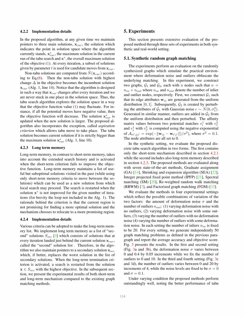
4.2.2 Implementation details
In the proposed algorithm, at any given time we maintain
pointers to three main solutions, xcur, the solution which
indicates the point in solution space where the algorithm
currently stands, x∗cur, the maximum solution in the current
run of the tabu search and x∗, the overall maximum solution
of the objective (1). At every iteration, a subset of solutions
given by parameter t is used for candidate moves from xcur.
Non-tabu solutions are computed from N(xcur) accord-
ing to Eq.(6). Then the non-tabu solution with highest
change ∆ in the objective becomes the incumbent solution
xcur (Alg. 1, line 14). Notice that the algorithm is designed
in such a way that xcur changes after every iteration and we
are never stuck in one place in the solution space. Thus, the
tabu search algorithm explores the solution space in a way
that the objective function value (1) may fluctuate. For in-
stance, if all the potential moves have negative value, then
the objective function will decrease. The solution x∗cur is
updated when the new solution is larger. The proposed al-
gorithm also incorporates the exception, called aspiration
criterion which allows tabu move to take place. The tabu
solution becomes current solution if it is strictly bigger than
the maximum solution x∗cur (Alg. 1, line 10).
4.2.3 Long term memory
Long-term memory, in contrast to short-term memory, takes
into account the extended search history and is activated
when the short-term criterion fails to improve the objec-
tive function. Long-term memory maintains a list of use-
ful but suboptimal solutions visited in the past (while using
only short-term memory criteria to move between the so-
lutions) which can be used as a new solution from which
local search may proceed. The search is restarted when the
solution x∗ is not improved for the given number of itera-
tions (for brevity the loop not included in the Alg. 1). The
rationale behind the criterion is that the current region is
not promising for finding a more optimal solution and the
mechanism chooses to relocate to a more promising region.
4.2.4 Implementation details
Various criteria can be adopted to make the long-term mem-
ory list. We implement long term memory as a list of “sec-
ond” solutions Ssec [3] which consists of solutions that at
every iteration landed just behind the current solution xcur,
called the “second” solution list . Therefore, in the algo-
rithm we also maintain pointers to a secondary solution xsec
which, if better, replaces the worst solution in the list of
secondary solutions. When the long-term termination cri-
terion is activated, a search is restarted from the solution
x ∈ Ssec with the highest objective. In the subsequent sec-
tion, we present the experimental results of both short-term
and long-term mechanism compared to the existing graph
matching methods.
5. Experiments
This section presents extensive evaluation of the pro-
posed method through three sets of experiments in both syn-
thetic and real-world setting.
5.1. Synthetic random graph matching
The experiments perform an evaluation on the randomly
synthesized graphs which simulate the practical environ-
ment where deformation noise and outliers obfuscate the
underlying matching. In this experiment, we construct
two graphs, G1 and G2, each with n nodes such that n =nin + nout where nin and nout denote the number of inlier
and outlier nodes, respectively. First, we construct G1 such
that its edge attributes wij are generated from the uniform
distribution [0, 1]. Subsequently, G2 is created by perturb-
ing the attributes of G1 with Gaussian noise ǫ ∼ N(0, σ2s).
Generated in similar manner, outliers are added in G2 from
the uniform distribution and then perturbed. The affinity
matrix values between two potential matches v1i with v2i′and v1j with v2j′ is computed using the negative exponential
of Aii′;jj′ = exp(−‖wij −wi′j′‖)/σ2), where σ2 = 0.1.
The node attributes are all set to 0.
In the synthetic setting, we evaluate the proposed dis-
crete tabu search algorithm in two forms. The first contains
only the short-term mechanism described in section 4.2.1
while the second includes also long-term memory described
in section 4.2.3. The proposed methods are evaluated along
with seven state-of-the-art methods, Graduate assignment
(GA) [14], Shrinking and expansion algorithm (SEA) [22],
Integer projected fixed point method (IPFP) [21], Spectral
matching (SM) [20], Re-weighted random walk matching
(RRWM) [7], and Factorized graph matching (FGM) [32].
We evaluate the methods in four experimental settings
which reflect the possible combinations of variation of the
two factors: the amount of deformation noise σ and the
number of outliers nout: (1) varying deformation noise with
no outliers, (2) varying deformation noise with some out-
liers, (3) varying the number of outliers with no deformation
noise (4) varying the number of outliers with some deforma-
tion noise. In each setting the number of inliers nin is fixed
to be 20. For every setting, we generate independently 50
graph matching problems as defined in the previous para-
graph and report the average accuracy and objective score.
Fig. 3 presents the results. In the first and second setting
(Fig. 3a and 3b), the deformation noise σ varies between
0 and 0.4 by 0.05 increments while we fix the number of
outliers to 0 and 10. In the third and fourth setting (Fig. 3c
and 3d), the number of outliers varies between 0 and 20 by
increments of 4, while the noise levels are fixed to be σ = 0and σ = 0.1.
Under varying condition the proposed methods perform
outstandingly well, noting the better performance of tabu
6114

(a) Varying deformation with no
outliers
(b) Varying deformation with
some outliers
(c) Varying outliers with no
deformation
(d) Varying outliers with some
deformation
Figure 3. Accuracy and score curves are plotted for four different conditions: varying the amount of deformation noise with fixed number
of outliers (a) nout = 0 and (b) nout = 10, and varying the number of outliers with fixed deformation noise (c) σ = 0 (d) σ = 0.15)
Table 2. SNU Dataset Average Accuracy (%)
Alg SEA GAGM RRWM IPFP Ours
Accuracy(%) 56.3 70.3 73.6 74.1 79.0
Time(s) 3.33 1.78 0.22 0.10 0.69
Table 3. Willow Object Dataset Average Accuracy (%)
Class Car Duck FaceMotor
bike
Wine
bottleavg
SEA 30.3 26.5 72.9 32.4 45.4 41.4
GAGM 38.6 35.4 79.4 38.3 53.9 49.1
RRWM 38.0 35.7 78.3 40.4 53.7 49.2
IPFP 37.6 36.9 80.4 40.4 56.0 50.3
Ours 39.5 36.1 80.2 44.0 57.9 51.5
search which includes only short-term memory. As the only
evaluated method, it achieves 100% accuracy given high
levels of noise (σ = 0.2 and σ = 0.25 with no outliers
and σ = 0.1 σ = 0.15 with outliers). While varying out-
liers, the method slightly falls short to SEA, whose perfor-
mance, however, considerably deteriorates when noise ap-
pears. The proposed method proves to be particularly robust
in more practical settings where both outliers and noise are
present. Given choice of parameters from Table 4.2.1 and
varying endIt and sol, it obtains superior solutions in the
presence of noise and outliers in 1.0-4.4 sec.; FGM - 23.5,
RRWM - 0.2, IPFP - 0.2, GAGM - 0.4 and SEA - 1.1 (aver-
aged results for results in Fig. 3b,d).
5.2. Real image feature correspondence
In this section, we evaluate the proposed method for fea-
ture correspondence task on two datasets: SNU dataset [7]
and Willow Object Class dataset [5]. RRWM, IPFP,
Model graph Proposed method IPFP
RRWM GAGM SEA
Model graph Proposed method IPFP
RRWM GAGM SEA
Figure 4. Example results of the real image matching on Willow
Object dataset. Keypoints are distinguished by different colors in
the model image and the matched locations are depicted for each
algorithm
GAGM, and SEA are compared with the proposed method3.
SNU dataset consists of 30 pairs of images most of which
are collected from Caltech-101 [10] and MSRC [1] dataset.
Each pair of images have similar viewpoints with large
3FGM is not compared because it cannot be applied in the experimental
setting of [7], which uses initial candidate matches.
7115

(a) Varying deformation with no
outliers
(b) Varying deformation with
some outliers
(c) Varying outliers with no
deformation
(d) Varying outliers with some
deformation
Figure 5. Accuracy and score curves are plotted for four different conditions: varying the amount of deformation noise with fixed number
of outliers (a) nout = 0 and (b) nout = 10, and varying the number of outliers with fixed deformation noise (c) σ = 0 (d) σ = 0.1).
intra-class variation. In addition to the original experimen-
tal setting [7], which did not use unary score, WHO [16]
and their inner product are used as feature descriptor and
unary score to enhance the overall performance. The aver-
age accuracy over 10 experiments is shown in Table 2. The
proposed algorithm outperforms all the other methods.
Willow dataset consists of 5 classes, whose images are
collected from Caltech-256 [15] and PASCAL VOC2007
dataset [9] with 10 manual keypoint annotation for each
image. Each class contains 40 to 108 images taken from
various viewpoints with clutter, making feature correspon-
dence extremely challenging. Therefore, we restricted the
graph constructed from one side image to have only key-
points without outliers. WHO [16] and HARG [5] are used
as node and edge descriptors, respectively. The average ac-
curacy over 100 random pairs is shown in Table 3. Classes
with low intra-class variation (face and winebottle) show
high accuracy overall, while the performance of the classes
with large intra-class variation (car, duck, and motorbike)
is relatively low. The proposed algorithm outperforms the
other algorithms in car, motorbike and winebottle classes,
while is comparable in face and duck classes. Some qual-
itative example results are shown in Fig. 4. The average
running times are following: proposed - 0.93s, RRWM -
0.04s, IPFP - 0.03s, GAGM - 0.08s, SEA - 0.49s.
5.3. Repeated Structure Matching
In this set of experiments, we present particular suit-
ability of tabu search method to multiple graph matching,
attempting to discover repeated structures or multiple in-
stances of an object. The advantage is due to the fact that
the method produces multiple solutions (Alg. 1, line 2-3),
each of which is a set of matches between two regions in
two graphs. The multiple solutions may or may not cor-
respond to the same regions in the original graphs. This
setting makes graph matching more useful in practical ap-
plications. E.g., in feature correspondence, it overcomes the
conventional restriction to allow one object per image.
In this set of experiments, we simulate the multiple ob-
ject environment. We construct Gmult1 and Gmult
2 according
to the procedure in Section (5.1) where |Gmult1 | = n and
|Gmult2 | = 2|Gmult
1 | = 2n in such a way that Gmult1 con-
sists of two independently perturbed copies of Gmult1 . The
affinity matrix Amult has size 2n2× 2n2. We subsequently
perform tabu search optimization on the penalized associa-
tion graph APmult obtained from Amult.
We compare our method to SEA which also produces
multiple solutions and the remaining methods evaluated in
Section (5.1) (with the exception of FGM whose running
time is too large for this set of experiments) adapted to mul-
tiple matching setting by means of the following sequential
matching procedure. We perform matching m times (where
m = 2 in our case) after each stage removing matched
nodes and performing the subsequent round on the remain-
ing nodes. The methods are evaluated in the same settings
as in Section (5.1) where we vary deformation noise and
the number of outliers. The results are presented in Fig. 5.
The proposed method outperforms the existing methods by
large margin when noise is varied. The improving accuracy
of SEA with the increasing number of outliers is notewor-
thy. The proposed method again performs very robustly in
a mixed environment with both noise and outliers present.
6. Conclusion
In this work, we propose graph matching algorithm
which adapts tabu search to search discrete solution space
directly and effectively. First, we build the framework based
on penalized association graph to move between its sub-
graphs by forbidding certain solutions and encouraging oth-
ers. As a result unlike any of the existing works, this method
works both in discrete space (by itself discrete graph match-
ing optimization is rare) and incorporates one-to-one con-
straint softly into the optimization process with no post-
processing step. The proposed method is suitable for mul-
tiple graph matching as it produces different solutions that
potentially correspond to repeated instances of an object.
The algorithm proves to be outstandingly robust achieving
superior results to the existing algorithms (in some cases
over 40 percentage points, which given a long history of
graph matching research, is notable) in the extensive combi-
nation of experiments where noise and outliers are present.
8116

References
[1] Microsoft research cambridge object recog-
nition image database. http://www.pascal-
network.org/challenges/VOC/voc2007/workshop/index.html.
7
[2] A. Albarelli, S. R. Bulo, A. Torsello, and M. Pelillo. Match-
ing as a non-cooperative game. In ICCV, 2009. 1
[3] R. Aringhieri, R. Cordone, and Y. Melzani. Tabu search ver-
sus grasp for the maximum diversity problem. 4OR, 2008.
6
[4] A. C. Berg, T. L. Berg, and J. Malik. Shape matching and
object recognition using low distortion correspondences. In
CVPR, 2005. 1
[5] M. Cho, K. Alahari, and J. Ponce. Learning graphs to match.
In ICCV, 2013. 7, 8
[6] M. Cho and J. Lee. Feature correspondence and deformable
object matching via agglomerative correspondence cluster-
ing. In ICCV, 2009. 1
[7] M. Cho, J. Lee, and K. M. Lee. Reweighted random walks
for graph matching. In ECCV, 2010. 1, 6, 7, 8
[8] O. Duchenne, A. Joulin, and J. Ponce. A graph-matching
kernel for object categorization. In ICCV, 2011. 1
[9] M. Everingham, L. Van Gool, C. K. I. Williams, J. Winn,
and A. Zisserman. The PASCAL Visual Object Classes
Challenge 2007 (VOC2007) Results. http://www.pascal-
network.org/challenges/VOC/voc2007/workshop/index.html.
8
[10] L. Fei-Fei, R. Fergus, and P. Perona. Learning generative
visual models from few training examples: An incremental
bayesian approach tested on 101 object categories. CVIU,
2007. 7
[11] F. Glover. Future paths for integer programming and links to
artificial intelligence. Computers and Operations Research,
1986. 4
[12] F. Glover. Tabu search-part i. ORSA Journal on Computing,
1989. 4
[13] F. Glover and M. Laguna. Tabu search. Springer, 1999. 1, 2,
4
[14] S. Gold and A. Rangarajan. A graduated assignment algo-
rithm for graph matching. TPAMI, 1996. 1, 6
[15] G. Griffin, A. Holub, and P. Perona. Caltech-256 object cat-
egory dataset. 2007. 8
[16] B. Hariharan, J. Malik, and D. Ramanan. Discriminative
decorrelation for clustering and classification. In ECCV.
2012. 8
[17] R. Horaud and T. Skordas. Stereo correspondence through
feature grouping and maximal cliques. TPAMI, 1989. 2
[18] S. Kim, S. Kwak, J. Feyereisl, and B. Han. Online multi-
target tracking by large margin structured learning. In ACCV.
2013. 1
[19] J. Lee, M. Cho, and K. M. Lee. A graph matching algorithm
using data-driven markov chain monte carlo sampling. In
ICPR, 2010. 1, 2
[20] M. Leordeanu and M. Hebert. A spectral technique for cor-
respondence problems using pairwise constraints. In ICCV,
2005. 1, 6
[21] M. Leordeanu and M. Hebert. An integer projected fixed
point method for graph matching and map inference. In
NIPS, 2009. 1, 2, 6
[22] H. Liu, L. J. Latecki, and S. Yan. Fast detection of dense
subgraphs with iterative shrinking and expansion. TPAMI,
2013. 2, 6
[23] H. Liu and S. Yan. Common visual pattern discovery via
spatially coherent correspondences. In CVPR, 2010. 2
[24] S. Sorlin and C. Solnon. Reactive tabu search for measuring
graph similarity. In Graph-Based Representations in Pattern
Recognition. Springer, 2005. 2
[25] Y. Suh, K. Adamczewski, and K. M. Lee. Subgraph match-
ing using compactness prior for robust feature correspo-
dence. In CVPR, 2015. 1
[26] Y. Suh, M. Cho, and K. M. Lee. Graph matching via sequen-
tial monte carlo. In ECCV, 2012. 1, 2
[27] S. Umeyama. An eigendecomposition approach to weighted
graph matching problems. TPAMI, 1988. 1
[28] Y. Wang, J.-K. Hao, F. Glover, and Z. Lu. A tabu search
based memetic algorithm for the maximum diversity prob-
lem. Engineering Applications of Artificial Intelligence,
2014. 4
[29] M. L. Williams, R. C. Wilson, and E. R. Hancock. Determin-
istic search for relational graph matching. Pattern Recogni-
tion, 1999. 2
[30] J. Yan, C. Zhang, H. Zha, W. Liu, X. Yang, and S. M. Chu.
Discrete hyper-graph matching. In CVPR, 2015. 1, 2
[31] Z. Zhao, Y. Qiao, J. Yang, and L. Bai. From dense subgraph
to graph matching: A label propagation approach. In Audio,
Language and Image Processing (ICALIP), 2014. 2
[32] F. Zhou and F. D. la Torre. Factorized graph matching. In
CVPR, 2012. 1, 2, 6
9117