Discrete Mechanical Interpolation of Keyframes

Thesis by

Weiwei Yang

In Partial Fulfillment of the Requirements

for the Degree of

Master of Science

California Institute of Technology

Pasadena, California

2007

(Submitted Dec 31, 2007)

ii

c© 2007

Weiwei Yang

All Rights Reserved

iii

Acknowledgments

To no absolutes; To Absolut.

iv

This page intentionally left blank.

v

Abstract

Advances in computer hardware and software have made it possible to use physical simulation

methods to add unprecedented degrees of realism to computer animations. Unfortunately, the

reliance on such methods makes it difficult or even impossible to control the results in order to

achieve artistic goals. We present a method for allowing artistic control of physical realism by

interpolating between given keyframes. The method is based on the discrete Lagrange-d’Alembert

principle; we introduce additional ghost forces that are calculated to bring the system into the

configuration requested by the artist. We derive a cost function that when minimized ensures the

corresponding motion to be smooth and physical looking. We describe the implementation and show

an example of animating a multi-particle mass-spring system in 3D using our method.

vi

This page intentionally left blank.

vii

Contents

Acknowledgments iii

Abstract v

1 Introduction 1

2 Overview of Lagrangian Dynamics 2

2.1 Continuous Lagrangian dynamics . . . . . . . . . . . . . . . . . . . . . . . . . . . . . 2

2.2 Discrete Lagrangian . . . . . . . . . . . . . . . . . . . . . . . . . . . . . . . . . . . . 3

2.3 Lagrange-d’Alembert principle . . . . . . . . . . . . . . . . . . . . . . . . . . . . . . 5

3 Hamilton-Pontryagin-Based Simulation 7

4 Discrete Mechanical Interpolation 9

4.1 Ghost force . . . . . . . . . . . . . . . . . . . . . . . . . . . . . . . . . . . . . . . . . 9

4.2 DMOC method . . . . . . . . . . . . . . . . . . . . . . . . . . . . . . . . . . . . . . . 10

4.3 Criteria for ghost forces . . . . . . . . . . . . . . . . . . . . . . . . . . . . . . . . . . 11

4.4 Our approach . . . . . . . . . . . . . . . . . . . . . . . . . . . . . . . . . . . . . . . . 12

5 Implementation Details 14

5.1 Solver . . . . . . . . . . . . . . . . . . . . . . . . . . . . . . . . . . . . . . . . . . . . 14

5.2 Regularization . . . . . . . . . . . . . . . . . . . . . . . . . . . . . . . . . . . . . . . 14

5.3 Relaxation . . . . . . . . . . . . . . . . . . . . . . . . . . . . . . . . . . . . . . . . . . 16

6 Examples 19

6.1 A simple 1-D mass spring system . . . . . . . . . . . . . . . . . . . . . . . . . . . . . 19

6.2 Coupled mass-spring system in 3-space . . . . . . . . . . . . . . . . . . . . . . . . . . 21

7 Discussion about TRACKS 27

8 Conclusion and Future Work 28

viii

This page intentionally left blank.

ix

List of Figures

2.1 Least action principle . . . . . . . . . . . . . . . . . . . . . . . . . . . . . . . . . . . 3

2.2 Discrete forces and momenta . . . . . . . . . . . . . . . . . . . . . . . . . . . . . . . 5

4.1 Simulation results vs. desired animation . . . . . . . . . . . . . . . . . . . . . . . . . 9

4.2 Discrete force and momentum distribution along a motion path. . . . . . . . . . . . 10

4.3 Possible motions containing two key frames . . . . . . . . . . . . . . . . . . . . . . . 11

4.4 Iterative process of finding middle frames . . . . . . . . . . . . . . . . . . . . . . . . 13

5.1 Pseudocode of our physical interpolation scheme. . . . . . . . . . . . . . . . . . . . . 15

5.2 Regularization by attaching fictitious springs . . . . . . . . . . . . . . . . . . . . . . 16

5.3 Relaxation process . . . . . . . . . . . . . . . . . . . . . . . . . . . . . . . . . . . . . 17

6.1 1-D mass-spring system. . . . . . . . . . . . . . . . . . . . . . . . . . . . . . . . . . . 19

6.2 Results for 1-D mass spring system . . . . . . . . . . . . . . . . . . . . . . . . . . . . 20

6.3 Resulting motion for non-physical key frames . . . . . . . . . . . . . . . . . . . . . . 21

6.4 Relaxation comparison . . . . . . . . . . . . . . . . . . . . . . . . . . . . . . . . . . . 22

6.5 Coupled mass-spring system. . . . . . . . . . . . . . . . . . . . . . . . . . . . . . . . 22

6.6 Key frames for coupled mass spring animation. . . . . . . . . . . . . . . . . . . . . . 22

6.7 Letter “D” to letter “M” . . . . . . . . . . . . . . . . . . . . . . . . . . . . . . . . . . 24

6.8 Letter “M” to letter “O” . . . . . . . . . . . . . . . . . . . . . . . . . . . . . . . . . . 25

6.9 Letter “O” to letter “C” . . . . . . . . . . . . . . . . . . . . . . . . . . . . . . . . . . 26

x

This page intentionally left blank.

1

Chapter 1

Introduction

The strive for realism in computer animation has made the task of animating objects such as hair,

smoke and water increasingly difficult and impractical. On the other hand, simulating such objects

using physics leaves little room for artistry: once initial conditions are set, the resulting simulations

are at the complete mercy of the underlying physics and numerical integrators. Furthermore, these

systems are usually highly nonlinear, and therefore make tweaking initial conditions to achieve

desired results a black art. For example, a simulated skirt may flow realistically around a character,

but it may also contain visually distracting creases that are impossible to iron out without changing

the material properties of the skirt. What it is needed is a scheme that allows artistic control of

physical realism.

In this thesis, we present an interpolation scheme based on the discrete Lagrange-d’Alembert

principle. Our goal is to provide a range of compromises between artistic control and the laws of

physics. We expect to see stylized, yet “physical looking” animation.

In chapter 2, we give an overview of Lagrangian dynamics, which is the foundation for our method.

In chapter 3, we describe the Hamilton-Pontryagin-based simulation method, which uses Lagrangian

dynamics to simulate physical materials such as a rubbery, elastic bunny. In chapter 4 we present

our method for interpolating keyframes based on discrete mechanics. Our implementation details

are covered in chapter 5. Chapter 6 contains results of animating coupled spring-mass systems using

our method.

2

Chapter 2

Overview of Lagrangian Dynamics

What follows is a brief overview of Lagrangian dynamics; for a more detailed description and deriva-

tion, please refer to Matthew West’s Ph.D. thesis [26] on variational integrators.

2.1 Continuous Lagrangian dynamics

Let q = (q1, q2, q3, . . . , qn) be the instantaneous configuration, or state, of a dynamical system in

Rn, and let q be the time derivative of q, q(t) = dq/dt. The Lagrangian L of the system is given as

a function of q and q and is defined as kinetic energy, K, minus potential energy, W :

L(q, q) = K(q(t)) − W (q(t)). (2.1)

The principle of stationary action states that, when the system is conservative, the motion of the

system from time t1 to t2 is such that the line integral

I(q) =

∫ t2

t1

L(q(t), q(t)) dt, (2.2)

which is called action, is stationary with respect to the variation of q for the correct path of the

motion between the fixed end points q(t1) = q1 and q(t2) = q2. In other words, the motion is such

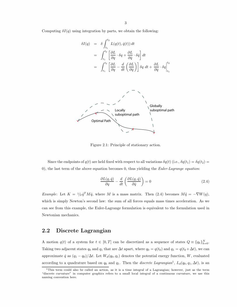
that the variation of the line integral I for fixed t1 and t2 is zero, as shown in figure (2.1):

δI(q) = δ

∫ t2

t1

L(q(t), q(t)) dt = 0 (2.3)

3

Computing δI(q) using integration by parts, we obtain the following:

δI(q) = δ

∫ t2

t1

L(q(t), q(t)) dt

=

∫ t2

t1

[

∂L

∂q· δq +

∂L

∂q· δq

]

dt

=

∫ t2

t1

[

∂L

∂q−

d

dt

(

∂L

∂q

)]

δq dt +∂L

∂q· δq

∣

∣

∣

∣

t2

t1

Globally

suboptimal pathLocally

suboptimal path

Optimal Path

Figure 2.1: Principle of stationary action.

Since the endpoints of q(t) are held fixed with respect to all variations δq(t) (i.e., δq(t1) = δq(t2) =

0), the last term of the above equation becomes 0, thus yielding the Euler-Lagrange equation:

∂L(q, q)

∂q−

d

dt

(

∂L(q, q)

∂q

)

= 0 (2.4)

Example: Let K = 1/2 qT Mq, where M is a mass matrix. Then (2.4) becomes Mq = −∇W (q),

which is simply Newton’s second law: the sum of all forces equals mass times acceleration. As we

can see from this example, the Euler-Lagrange formulation is equivalent to the formulation used in

Newtonian mechanics.

2.2 Discrete Lagrangian

A motion q(t) of a system for t ∈ [0, T ] can be discretized as a sequence of states Q ≡ {qk}Nk=0

.

Taking two adjacent states q0 and q1 that are ∆t apart, where q0 = q(t0) and q1 = q(t0 +∆t), we can

approximate q as (q1 − q0)/∆t. Let Wd(q0, q1) denotes the potential energy function, W , evaluated

according to a quadrature based on q0 and q1. Then the discrete Lagrangian1, Ld(q0, q1, ∆t), is an

1This term could also be called an action, as it is a time integral of a Lagrangian; however, just as the term

“discrete curvature” in computer graphics refers to a small local integral of a continuous curvature, we use this

naming convention here.

4

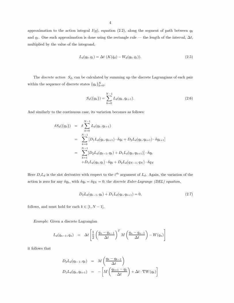
approximation to the action integral I(q), equation (2.2), along the segment of path between q0

and q1. One such approximation is done using the rectangle rule — the length of the interval, ∆t,

multiplied by the value of the integrand,

Ld(q0, q1) = ∆t (K(qd) − Wd(q0, q1)). (2.5)

The discrete action Sd, can be calculated by summing up the discrete Lagrangians of each pair

within the sequence of discrete states {qk}Nk=0

,

Sd({qk}) =

N−1∑

k=0

Ld(qk, qk+1). (2.6)

And similarly to the continuous case, its variation becomes as follows:

δSd({qk}) = δN−1∑

k=0

Ld(qk, qk+1)

=

N−1∑

k=0

[D1Ld(qk, qk+1) · δqk + D2Ld(qk, qk+1) · δqk+1]

=

N−1∑

k=1

[D2Ld(qk−1, qk) + D1Ld(qk, qk+1)] · δqk

+D1Ld(q0, q1) · δq0 + D2Ld(qN−1, qN ) · δqN

Here DiLd is the slot derivative with respect to the ith argument of Ld. Again, the variation of the

action is zero for any δqk, with δq0 = δqN = 0; the discrete Euler-Lagrange (DEL) equation,

D2Ld(qk−1, qk) + D1Ld(qk, qk+1) = 0, (2.7)

follows, and must hold for each k ∈ [1, N − 1].

Example: Given a discrete Lagrangian

Ld(qn−1, qn) = ∆t

[

1

2

(

qn − qn−1

∆t

)T

M

(

qn − qn−1

∆t

)

− W (qn)

]

it follows that

D2Ld(qk−1, qk) = M

(

qk − qk−1

∆t

)

D1Ld(qk, qk+1) = −

[

M

(

qk+1 − qk

∆t

)

+ ∆t · ∇W (qk)

]

5

and (2.7) becomes the discretization of Newton’s second law:

M

(

qk+1 − 2qk + qk−1

(∆t)2

)

= −∇W (qk).

2.3 Lagrange-d’Alembert principle

Non-conservative systems, which contain forcing or dissipating terms, can be described using the

Lagrange-d’Alembert principle in the continuous case, where F (q(t), q(t)) is the non-conservative

force:

δ

∫

L(q(t), q(t)) dt +

∫

F (q(t), q(t)) · δq dt = 0 (2.8)

The discrete Lagrange-d’Alembert principle states that

δ

N−1∑

k=0

Ld(qk, qk+1) +

N−1∑

k=0

[F−

d (qk, qk+1) · δqk + F+

d (qk, qk+1) · δqk+1] = 0. (2.9)

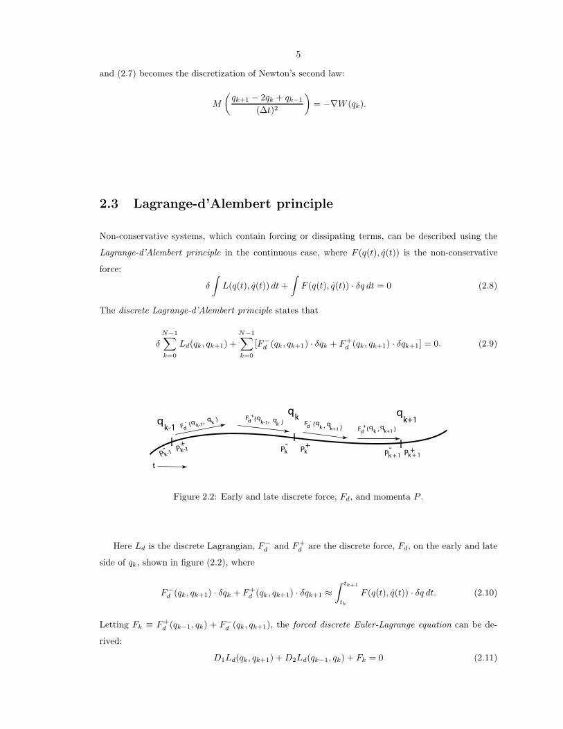
qk k+1

q

Pk+

Pk-

qk-1 Fd

- ( , )q

k-1q

k

Pk-1+

Pk-1- Pk + 1

+Pk + 1-

Fd

+( , )q

k-1q

k Fd

-( , )q

kq

k+1 Fd+

( , )qk

qk+1

t

Figure 2.2: Early and late discrete force, Fd, and momenta P .

Here Ld is the discrete Lagrangian, F−

d and F+

d are the discrete force, Fd, on the early and late

side of qk, shown in figure (2.2), where

F−

d (qk, qk+1) · δqk + F+

d (qk, qk+1) · δqk+1 ≈

∫ tk+1

tk

F (q(t), q(t)) · δq dt. (2.10)

Letting Fk ≡ F+

d (qk−1, qk) + F−

d (qk, qk+1), the forced discrete Euler-Lagrange equation can be de-

rived:

D1Ld(qk, qk+1) + D2Ld(qk−1, qk) + Fk = 0 (2.11)

6

Let’s define the early and late momenta at time step k as follows:

p+

k = −D1Ld(qk, qk+1) − F−

d (qk, qk+1) (2.12)

p−k = D2Ld(qk−1, qk) + F+

d (qk−1, qk) (2.13)

(2.14)

Now the DEL equation, (2.11), can be rewritten simply as

p+

k − p−k = 0. (2.15)

7

Chapter 3

Hamilton-Pontryagin-Based

Simulation

Let us now sketch the method for physically based simulation presented by Kharevych et al. [13]

based on the Hamilton-Pontryagin Principle, which states that

δ

∫ T

0

[p(q − v) + L(q, v)] dt = 0 (3.1)

For more details on this method, and our novel update through minimization please refer to the

paper.

In the Hamilton-Pontryagin Principle, the configuration variable q, the velocity v, and the mo-

mentum p are treated as independent variables, that is q(t), v(t), and p(t) vary independently with

end-point conditions on q(t). Taking the variation of the three independent variables, δp(t), δq(t)

and δv(t) yields that

v = q,dp

dt=

∂L(q, v)

∂q, and p =

∂L(q, v)

∂v. (3.2)

Time Discretization Similar to the discretization of q(t) as the sequence {qk}Nk=0

, v(t) and p(t)

are discretized by the sequences {vk}Nk=1

and {pk}Nk=1

. Velocities vk+1 and momenta pk+1 are viewed

as approximations within the intervals [tk, tk+1], which are staggered with respect to the positions

qk. We will call hk the time step between time tk and tk+1. Even though the time step can be

adjusted throughout the computation based on standard time step control ideas, it is observed in

practice that the numerics of a simulation are more stable when hk is fixed in time.

Discrete Hamilton-Pontryagin Principle Once a discrete Lagrangian in the form of (2.5) is

given, then its corresponding discrete Hamilton-Pontryagin principle can be expressed as follows:

δN∑

k=0

[

pk+1

(

qk+1 − qk

hk

− vk+1

)

hk + Ld(qk, vk+1)

]

= 0 (3.3)

8

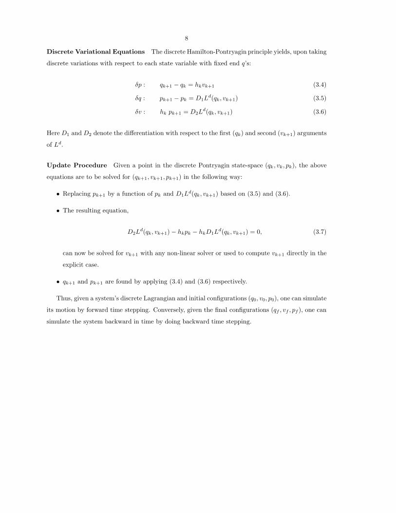
Discrete Variational Equations The discrete Hamilton-Pontryagin principle yields, upon taking

discrete variations with respect to each state variable with fixed end q’s:

δp : qk+1 − qk = hkvk+1 (3.4)

δq : pk+1 − pk = D1Ld(qk, vk+1) (3.5)

δv : hk pk+1 = D2Ld(qk, vk+1) (3.6)

Here D1 and D2 denote the differentiation with respect to the first (qk) and second (vk+1) arguments

of Ld.

Update Procedure Given a point in the discrete Pontryagin state-space (qk, vk, pk), the above

equations are to be solved for (qk+1, vk+1, pk+1) in the following way:

• Replacing pk+1 by a function of pk and D1Ld(qk, vk+1) based on (3.5) and (3.6).

• The resulting equation,

D2Ld(qk, vk+1) − hkpk − hkD1L

d(qk, vk+1) = 0, (3.7)

can now be solved for vk+1 with any non-linear solver or used to compute vk+1 directly in the

explicit case.

• qk+1 and pk+1 are found by applying (3.4) and (3.6) respectively.

Thus, given a system’s discrete Lagrangian and initial configurations (q0, v0, p0), one can simulate

its motion by forward time stepping. Conversely, given the final configurations (qf , vf , pf ), one can

simulate the system backward in time by doing backward time stepping.

9

Chapter 4

Discrete Mechanical Interpolation

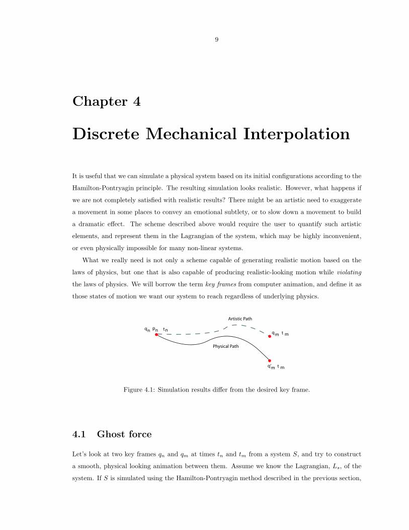
It is useful that we can simulate a physical system based on its initial configurations according to the

Hamilton-Pontryagin principle. The resulting simulation looks realistic. However, what happens if

we are not completely satisfied with realistic results? There might be an artistic need to exaggerate

a movement in some places to convey an emotional subtlety, or to slow down a movement to build

a dramatic effect. The scheme described above would require the user to quantify such artistic

elements, and represent them in the Lagrangian of the system, which may be highly inconvenient,

or even physically impossible for many non-linear systems.

What we really need is not only a scheme capable of generating realistic motion based on the

laws of physics, but one that is also capable of producing realistic-looking motion while violating

the laws of physics. We will borrow the term key frames from computer animation, and define it as

those states of motion we want our system to reach regardless of underlying physics.

qn pn

q‘m

qmtn

t m

t m

Physical Path

Artistic Path

Figure 4.1: Simulation results differ from the desired key frame.

4.1 Ghost force

Let’s look at two key frames qn and qm at times tn and tm from a system S, and try to construct

a smooth, physical looking animation between them. Assume we know the Lagrangian, Ls, of the

system. If S is simulated using the Hamilton-Pontryagin method described in the previous section,

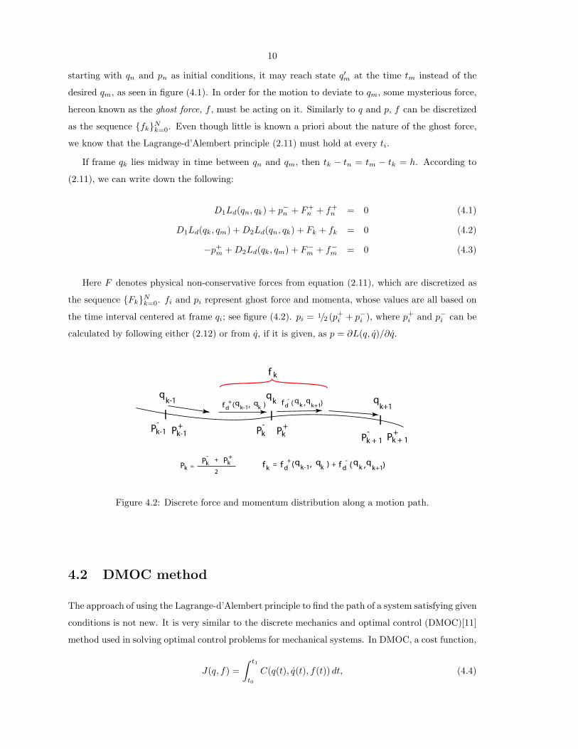
10

starting with qn and pn as initial conditions, it may reach state q′m at the time tm instead of the

desired qm, as seen in figure (4.1). In order for the motion to deviate to qm, some mysterious force,

hereon known as the ghost force, f , must be acting on it. Similarly to q and p, f can be discretized

as the sequence {fk}Nk=0

. Even though little is known a priori about the nature of the ghost force,

we know that the Lagrange-d’Alembert principle (2.11) must hold at every ti.

If frame qk lies midway in time between qn and qm, then tk − tn = tm − tk = h. According to

(2.11), we can write down the following:

D1Ld(qn, qk) + p−n + F+n + f+

n = 0 (4.1)

D1Ld(qk, qm) + D2Ld(qn, qk) + Fk + fk = 0 (4.2)

−p+m + D2Ld(qk, qm) + F−

m + f−

m = 0 (4.3)

Here F denotes physical non-conservative forces from equation (2.11), which are discretized as

the sequence {Fk}Nk=0

. fi and pi represent ghost force and momenta, whose values are all based on

the time interval centered at frame qi; see figure (4.2). pi = 1/2 (p+

i + p−i ), where p+

i and p−i can be

calculated by following either (2.12) or from q, if it is given, as p = ∂L(q, q)/∂q.

qk

k+1q

Pk+

Pk-

Pk =Pk

-Pk

++

2

qk-1

f d+

( , )qk-1

qk

f d-

( , )qk

qk+1

f d+

( , )qk-1

qk f d

-( , )q

kq

k+1f k= +

f k

Pk-1+Pk-1

-

Pk + 1+

Pk + 1-

Figure 4.2: Discrete force and momentum distribution along a motion path.

4.2 DMOC method

The approach of using the Lagrange-d’Alembert principle to find the path of a system satisfying given

conditions is not new. It is very similar to the discrete mechanics and optimal control (DMOC)[11]

method used in solving optimal control problems for mechanical systems. In DMOC, a cost function,

J(q, f) =

∫ t1

t0

C(q(t), q(t), f(t)) dt, (4.4)

11

is minimized under the constraint (2.8). This method is very efficient in finding a motion when the

mechanical systems involved only have a few degrees of freedom, (below a few hundreds). However,

it does not scale well and becomes inadequate for the types of physical systems we simulate in

computer animation, where we could have up to a few thousand degrees of freedom.

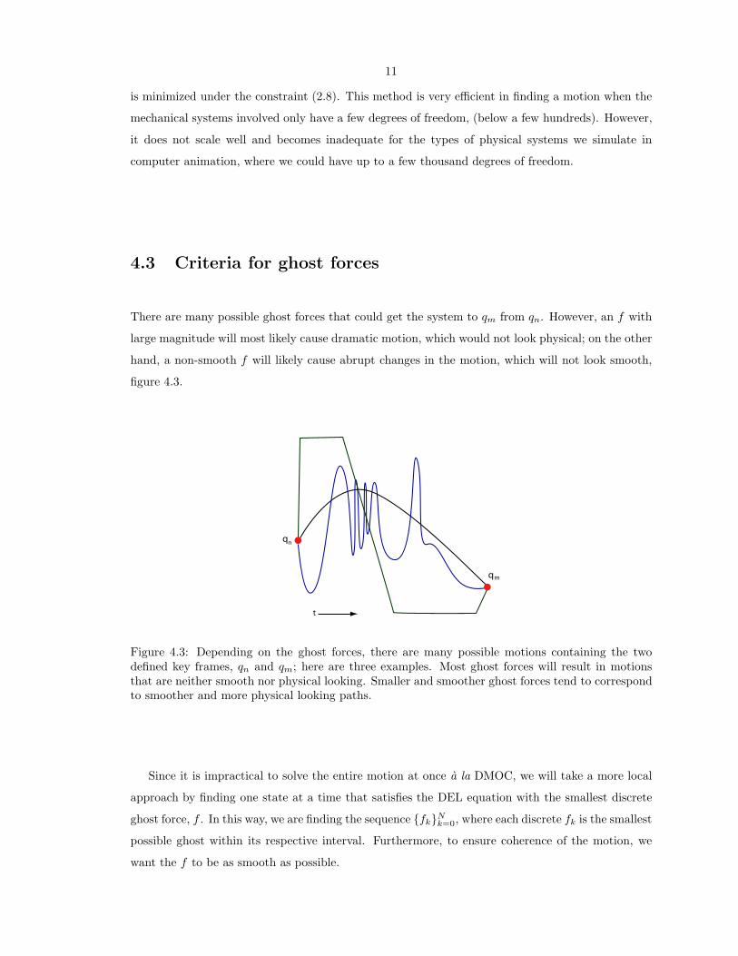
4.3 Criteria for ghost forces

There are many possible ghost forces that could get the system to qm from qn. However, an f with

large magnitude will most likely cause dramatic motion, which would not look physical; on the other

hand, a non-smooth f will likely cause abrupt changes in the motion, which will not look smooth,

figure 4.3.

qn

qm

t

Figure 4.3: Depending on the ghost forces, there are many possible motions containing the twodefined key frames, qn and qm; here are three examples. Most ghost forces will result in motionsthat are neither smooth nor physical looking. Smaller and smoother ghost forces tend to correspondto smoother and more physical looking paths.

Since it is impractical to solve the entire motion at once a la DMOC, we will take a more local

approach by finding one state at a time that satisfies the DEL equation with the smallest discrete

ghost force, f . In this way, we are finding the sequence {fk}Nk=0

, where each discrete fk is the smallest

possible ghost within its respective interval. Furthermore, to ensure coherence of the motion, we

want the f to be as smooth as possible.

12

4.4 Our approach

Let’s start by establishing some relation between fk and qk. To do this, we go back to the DEL

equations (4.1)–(4.3) and solve for each discrete fk:

f+n = D1Ld(qn, qk) + p−n + F+

n

fk = D1Ld(qk, qm) + D2Ld(qn, qk) + Fk

f−

m = −p+m + D2Ld(qk, qm) + F−

m

Each of these is of the form

fi = p+

i − p−i . (4.5)

This means that the smaller the difference between a pair of early and late discrete momenta, the

smaller the ghost force within that interval. This should not come as a surprise, since when there is

no ghost force present, p+

i − p−i = 0, (2.15). One way to minimize fi is to minimize its norm; here

we use the L2 norm. Incidentally, one way to ensure smoothness of f is by imposing the condition

that the difference between every adjacent f be as small as possible; in other words, the sum of all

L2 norm of the two differences, fi−1 − fi and fi+1 − fi, is minimized.

We define:

E(p−, p+, ∆t) =

(

p+ − p−

∆t

)2

∆t, (4.6)

which is the L2 norms of the difference p+−p−, where p+ and p− are both associated with the same

frame, normalized with respect to its corresponding time step. And

Es(f1, f2, ∆t) =

(

f2 − f1

∆t

)2

∆t, (4.7)

the L2 norm of the differences between fk, and its two adjacent ghost forces, f+n and f−

m, also

normalized with respect to its corresponding time step.

Let λs denote a constant that weighs the contribution of the smoothness versus the magnitude

of the ghost forces in the objective function. It can be adjusted according to desired results.

Now we are ready to define a cost function Jqk, that when minimized with respect to qk will give

us a sequence of small and smooth {fk}Nk=0

.

Jqk= E(pn + F+

n ,−D1Ld(qn, qk),hk

2) + E(D2Ld(qn, qk) + Fk,−D1Ld(qk, qm), hk) +(4.8)

+ E(D2Ld(qk, qm) + F−

m , pm,hk

2) + λs

(

Es(f+n ,

fk

2, hk) + Es(

fk

2, f−

m, hk)

)

There are three E terms in Jqk, since a change in the location of qk will affect not only p+

k , p−k ,

13

and their associated fk, but also p+n , p+

m, and f+n , f−

m.

For systems with more than two key frames, we repeat the minimization process on every two

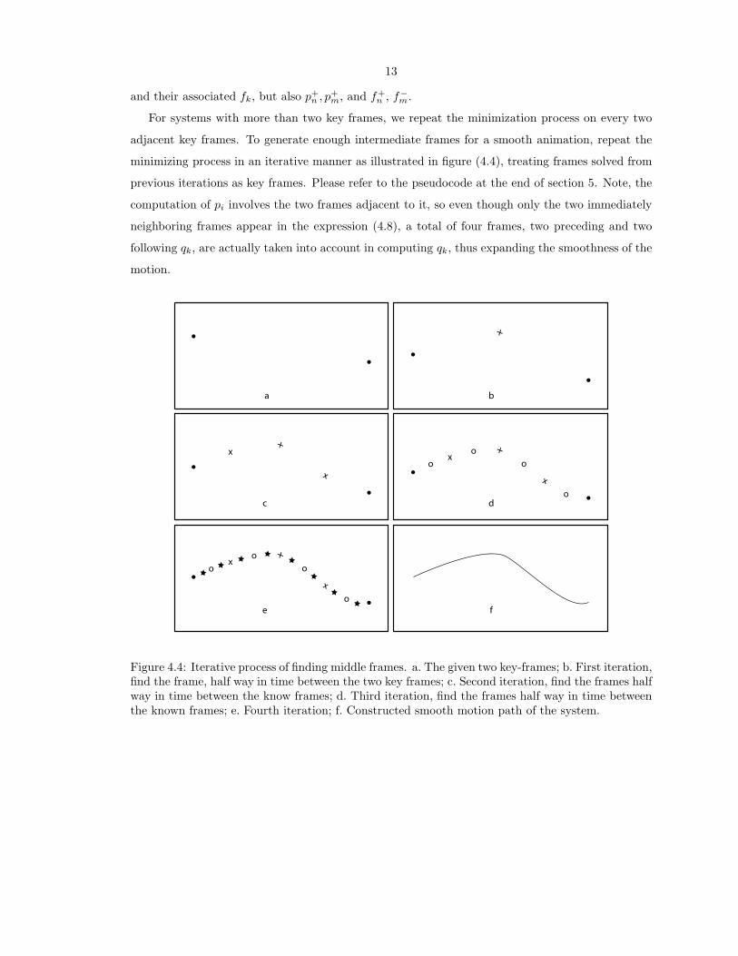
adjacent key frames. To generate enough intermediate frames for a smooth animation, repeat the

minimizing process in an iterative manner as illustrated in figure (4.4), treating frames solved from

previous iterations as key frames. Please refer to the pseudocode at the end of section 5. Note, the

computation of pi involves the two frames adjacent to it, so even though only the two immediately

neighboring frames appear in the expression (4.8), a total of four frames, two preceding and two

following qk, are actually taken into account in computing qk, thus expanding the smoothness of the

motion.

x

x

x

x

o

o

o

o

x

x

o

o

o

o

a b

c d

e f

Figure 4.4: Iterative process of finding middle frames. a. The given two key-frames; b. First iteration,find the frame, half way in time between the two key frames; c. Second iteration, find the frames halfway in time between the know frames; d. Third iteration, find the frames half way in time betweenthe known frames; e. Fourth iteration; f. Constructed smooth motion path of the system.

14

Chapter 5

Implementation Details

5.1 Solver

Any solver capable of handling non-linear system could be used. In our implementation, we used the

package Ipopt (Interior Point OPTimizer)[25]. Because the Hessian of the objective function (4.8)

contains second order derivatives, its analytical expression can become quite lengthy and prone to

human errors, especially for complicated potential functions W (qk). Therefore we opted to use the

built-in numerical Hessian approximation function in Ipopt.

5.2 Regularization

Since the objective functions, (4.8), are usually non-linear, it is not always easy to minimize them.

Another difficulty, especially in the initial steps where the time steps between frames, hk, are large,

is that the −hk∇W term dominates, making the gradient non-positive-definite. In the first few

iterations, we thus need to help the solver converge by adding a regularization term to (4.8). The

regularization term should vanish as hk between frames becomes small, so that the regularization

does not affect the motion of the system at finer levels. To ensure this, we write the regularization

term with a scalar factor c(hk), as c(hk)Ereg , where

limhk→0

c(hk) = 0.

There are many ways to regularize, depending on the system and desired results; any one method,

or a combination of all described below can be used.

Spatial Laplacian: It is observed in most physical systems that neighboring parts tend to move

in unison. When neighboring parts do not move in unison, the system exhibits shaking/jitteriness,

15

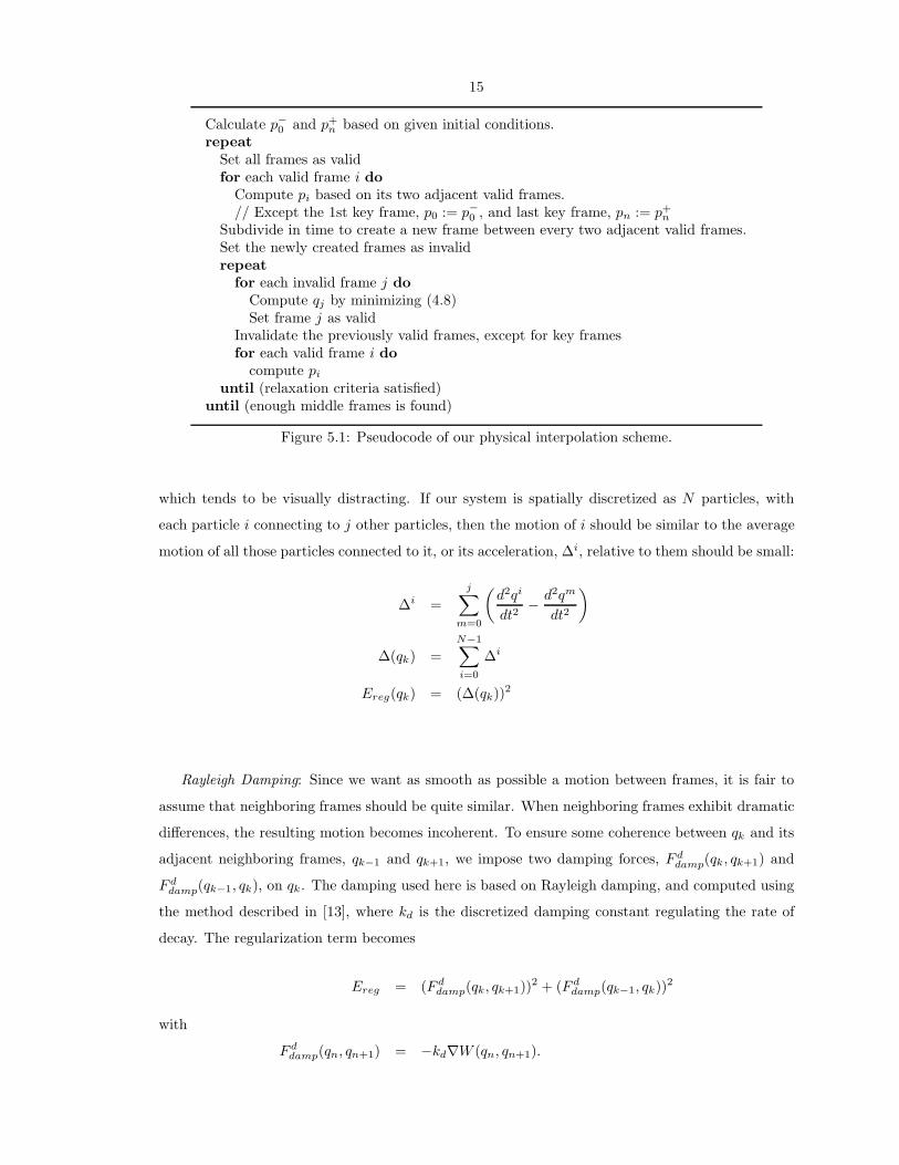
Calculate p−0 and p+n based on given initial conditions.

repeat

Set all frames as validfor each valid frame i do

Compute pi based on its two adjacent valid frames.// Except the 1st key frame, p0 := p−0 , and last key frame, pn := p+

n

Subdivide in time to create a new frame between every two adjacent valid frames.Set the newly created frames as invalidrepeat

for each invalid frame j do

Compute qj by minimizing (4.8)Set frame j as valid

Invalidate the previously valid frames, except for key framesfor each valid frame i do

compute pi

until (relaxation criteria satisfied)until (enough middle frames is found)

Figure 5.1: Pseudocode of our physical interpolation scheme.

which tends to be visually distracting. If our system is spatially discretized as N particles, with

each particle i connecting to j other particles, then the motion of i should be similar to the average

motion of all those particles connected to it, or its acceleration, ∆i, relative to them should be small:

∆i =

j∑

m=0

(

d2qi

dt2−

d2qm

dt2

)

∆(qk) =

N−1∑

i=0

∆i

Ereg(qk) = (∆(qk))2

Rayleigh Damping: Since we want as smooth as possible a motion between frames, it is fair to

assume that neighboring frames should be quite similar. When neighboring frames exhibit dramatic

differences, the resulting motion becomes incoherent. To ensure some coherence between qk and its

adjacent neighboring frames, qk−1 and qk+1, we impose two damping forces, F ddamp(qk, qk+1) and

F ddamp(qk−1, qk), on qk. The damping used here is based on Rayleigh damping, and computed using

the method described in [13], where kd is the discretized damping constant regulating the rate of

decay. The regularization term becomes

Ereg = (F ddamp(qk, qk+1))

2 + (F ddamp(qk−1, qk))2

with

F ddamp(qn, qn+1) = −kd∇W (qn, qn+1).

16

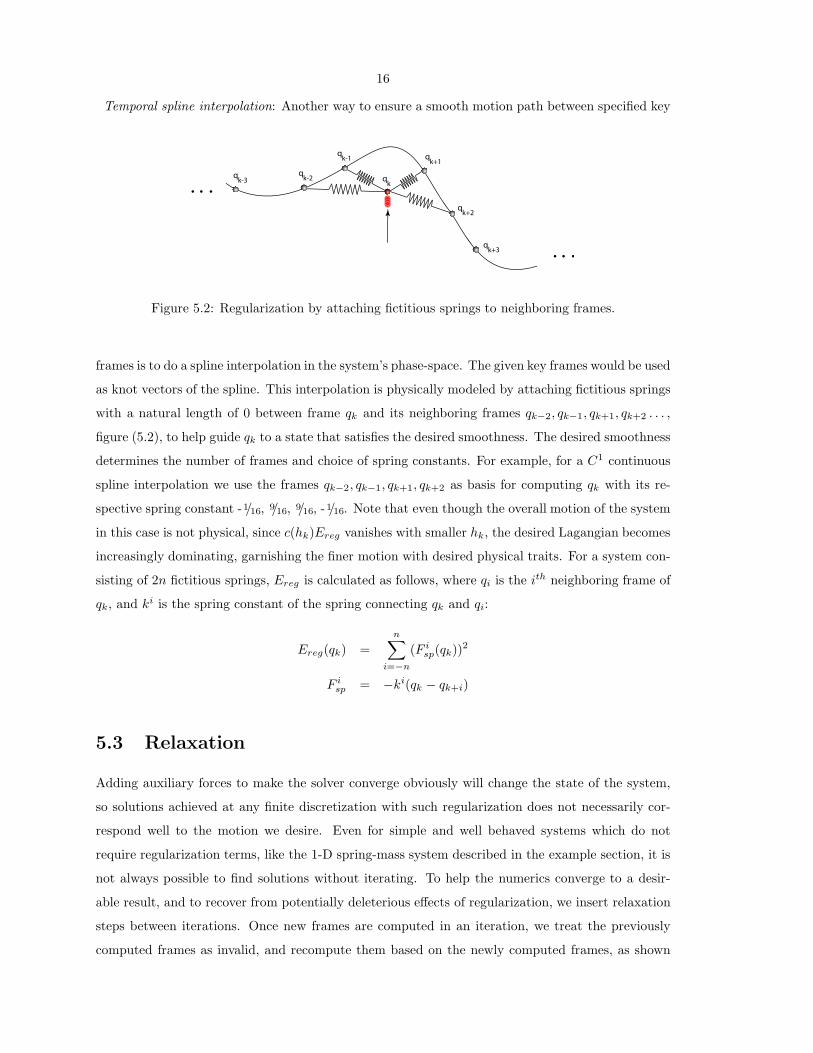
Temporal spline interpolation: Another way to ensure a smooth motion path between specified key

qk

qk-1 q

k+1

qk+2

qk+3

qk-2q

k-3

Figure 5.2: Regularization by attaching fictitious springs to neighboring frames.

frames is to do a spline interpolation in the system’s phase-space. The given key frames would be used

as knot vectors of the spline. This interpolation is physically modeled by attaching fictitious springs

with a natural length of 0 between frame qk and its neighboring frames qk−2, qk−1, qk+1, qk+2 . . . ,

figure (5.2), to help guide qk to a state that satisfies the desired smoothness. The desired smoothness

determines the number of frames and choice of spring constants. For example, for a C1 continuous

spline interpolation we use the frames qk−2, qk−1, qk+1, qk+2 as basis for computing qk with its re-

spective spring constant -1/16, 9/16, 9/16, -1/16. Note that even though the overall motion of the system

in this case is not physical, since c(hk)Ereg vanishes with smaller hk, the desired Lagangian becomes

increasingly dominating, garnishing the finer motion with desired physical traits. For a system con-

sisting of 2n fictitious springs, Ereg is calculated as follows, where qi is the ith neighboring frame of

qk, and ki is the spring constant of the spring connecting qk and qi:

Ereg(qk) =

n∑

i=−n

(F isp(qk))2

F isp = −ki(qk − qk+i)

5.3 Relaxation

Adding auxiliary forces to make the solver converge obviously will change the state of the system,

so solutions achieved at any finite discretization with such regularization does not necessarily cor-

respond well to the motion we desire. Even for simple and well behaved systems which do not

require regularization terms, like the 1-D spring-mass system described in the example section, it is

not always possible to find solutions without iterating. To help the numerics converge to a desir-

able result, and to recover from potentially deleterious effects of regularization, we insert relaxation

steps between iterations. Once new frames are computed in an iteration, we treat the previously

computed frames as invalid, and recompute them based on the newly computed frames, as shown

17

I II

III IV

VI V

Key frames Frame solved in previous iteration

Frames solved in current iteration Locations before relaxation

Desired Path Actual Path

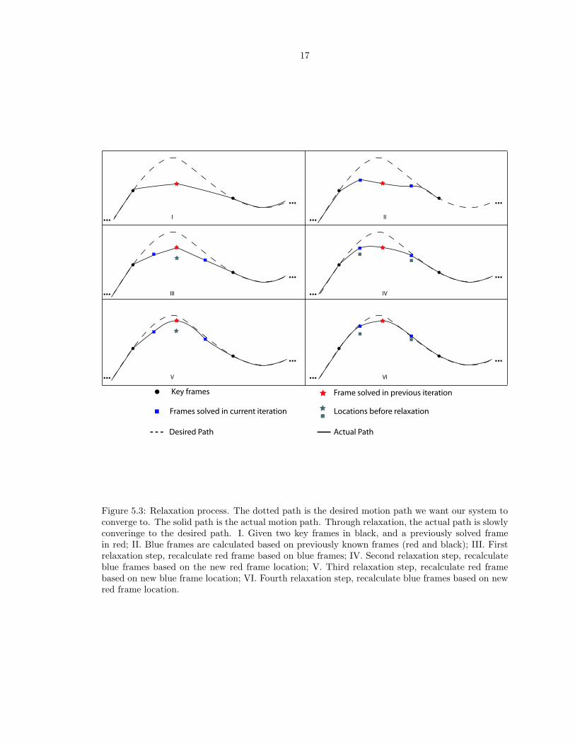
Figure 5.3: Relaxation process. The dotted path is the desired motion path we want our system toconverge to. The solid path is the actual motion path. Through relaxation, the actual path is slowlyconveringe to the desired path. I. Given two key frames in black, and a previously solved framein red; II. Blue frames are calculated based on previously known frames (red and black); III. Firstrelaxation step, recalculate red frame based on blue frames; IV. Second relaxation step, recalculateblue frames based on the new red frame location; V. Third relaxation step, recalculate red framebased on new blue frame location; VI. Fourth relaxation step, recalculate blue frames based on newred frame location.

18

in figure (5.3). This process can be repeated many times. The optimal number of relaxation steps

needed depends on the number of states in that system. The method used here is slow, as during

one relaxation step, a change to a frame will only be propagated to its two adjacent frames. To

help speed up the relaxation process, we employ an numerical trick along the principle of successive

over-relaxation [22]. If qo is the location of frame q before relaxation, and qn is the new location

after, then dq = qn − qo. Assuming dq is along the right direction for q to converge to, then we can

speed up the convergence process by introducing an over-relax factor cr, so instead of q = qo + dq,

we let q = qo + cr dq. It is best to keep cr ∈ [1, 2), as over shooting could happen which will result

in q unnecessarily oscillating around the value it is trying to converge to. An example of the effects

of relaxation on a motion path is given in the 1-D mass-spring example below.

19

Chapter 6

Examples

6.1 A simple 1-D mass spring system

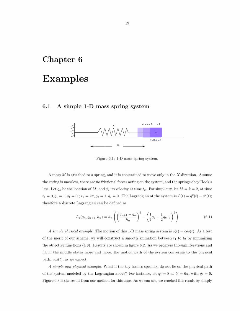
m

k

m

m = k = 2

t =0 , x = 1

l = 1

0

Figure 6.1: 1-D mass-spring system.

A mass M is attached to a spring, and it is constrained to move only in the X direction. Assume

the spring is massless, there are no frictional forces acting on the system, and the springs obey Hook’s

law. Let qk be the location of M , and qk its velocity at time tk. For simplicity, let M = k = 2, at time

t1 = 0, q1 = 1, q1 = 0 ; t2 = 2π, q2 = 1, q2 = 0. The Lagrangian of the system is L(t) = q2(t)− q2(t);

therefore a discrete Lagrangian can be defined as:

Ld(qn, qn+1, hn) = hn

(

(

qn+1 − qn

hn

)2

−

(

1

2qk +

1

2qk+1

)2)

(6.1)

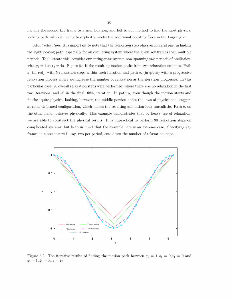
A simple physical example: The motion of this 1-D mass spring system is q(t) = cos(t). As a test

of the merit of our scheme, we will construct a smooth animation between t1 to t2 by minimizing

the objective functions (4.8). Results are shown in figure 6.2. As we progress through iterations and

fill in the middle states more and more, the motion path of the system converges to the physical

path, cos(t), as we expect.

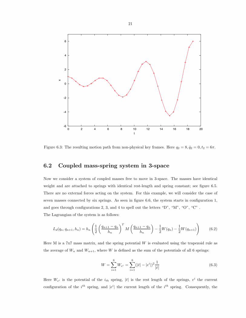
A simple non-physical example: What if the key frames specified do not lie on the physical path

of the system modeled by the Lagrangian above? For instance, let q2 = 8 at t2 = 6π, with q2 = 0.

Figure 6.3 is the result from our method for this case. As we can see, we reached this result by simply

20

moving the second key frame to a new location, and left to our method to find the most physical

looking path without having to explicitly model the additional boosting force in the Lagrangian.

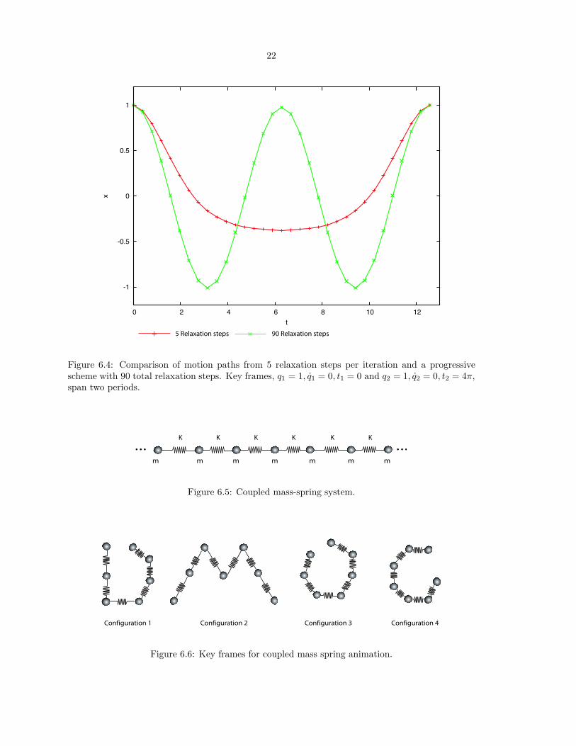
About relaxation: It is important to note that the relaxation step plays an integral part in finding

the right looking path, especially for an oscillating system where the given key frames span multiple

periods. To illustrate this, consider our spring-mass system now spanning two periods of oscillation,

with q2 = 1 at t2 = 4π. Figure 6.4 is the resulting motion paths from two relaxation schemes. Path

a, (in red), with 5 relaxation steps within each iteration and path b, (in green) with a progressive

relaxation process where we increase the number of relaxation as the iteration progresses. In this

particular case, 90 overall relaxation steps were performed, where there was no relaxation in the first

two iterations, and 40 in the final, fifth, iteration. In path a, even though the motion starts and

finishes quite physical looking, however, the middle portion defies the laws of physics and staggers

at some deformed configuration, which makes the resulting animation look unrealistic. Path b, on

the other hand, behaves physically. This example demonstrates that by heavy use of relaxation,

we are able to construct the physical results. It is impractical to perform 90 relaxation steps on

complicated systems, but keep in mind that the example here is an extreme case. Specifying key

frames in closer intervals, say, two per period, cuts down the number of relaxation steps.

-1

-0.5

0

0.5

1

0 1 2 3 4 5 6

x

t

First iteration Second iteration

Third iteration Fourth iteration

Fifith iteration

Figure 6.2: The iterative results of finding the motion path between q1 = 1, q1 = 0, t1 = 0 andq2 = 1, q2 = 0, t2 = 2π

21

-6

-4

-2

0

2

4

6

0 2 4 6 8 10 12 14 16 18 20

x

t

Figure 6.3: The resulting motion path from non-physical key frames. Here q2 = 8, q2 = 0, t2 = 6π.

6.2 Coupled mass-spring system in 3-space

Now we consider a system of coupled masses free to move in 3-space. The masses have identical

weight and are attached to springs with identical rest-length and spring constant; see figure 6.5.

There are no external forces acting on the system. For this example, we will consider the case of

seven masses connected by six springs. As seen in figure 6.6, the system starts in configuration 1,

and goes through configurations 2, 3, and 4 to spell out the letters “D”, “M”, “O”, “C” .

The Lagrangian of the system is as follows:

Ld(qn, qn+1, hn) = hn

(

1

2

(

qn+1 − qn

hn

)T

M

(

qn+1 − qn

hn

)

−1

2W (qn) −

1

2W (qn+1)

)

(6.2)

Here M is a 7x7 mass matrix, and the spring potential W is evaluated using the trapezoid rule as

the average of Wn and Wn+1, where W is defined as the sum of the potentials of all 6 springs:

W =

6∑

i=1

Wei =

6∑

i=1

(|e| − |ei|)21

|e|(6.3)

Here Wei is the potential of the ith spring, |e| is the rest length of the springs, ei the current

configuration of the ith spring, and |ei| the current length of the ith spring. Consequently, the

22

-1

-0.5

0

0.5

1

0 2 4 6 8 10 12

x

t

5 Relaxation steps 90 Relaxation steps

Figure 6.4: Comparison of motion paths from 5 relaxation steps per iteration and a progressivescheme with 90 total relaxation steps. Key frames, q1 = 1, q1 = 0, t1 = 0 and q2 = 1, q2 = 0, t2 = 4π,span two periods.

m m m m m m m

K K K K K K

Figure 6.5: Coupled mass-spring system.

Configuration 3Configuration 2Configuration 1 Configuration 4

Figure 6.6: Key frames for coupled mass spring animation.

23

partial derivatives of the Lagrangian are

D1Ld(qn, qn+1, hn) = −hn

(

M

(

qn+1 − qn

hn

)

+1

2∇W (qn)

)

and

D2Ld(qn, qn+1, hn) = hn

(

M

(

qn+1 − qn

hn

)

−1

2∇W (qn+1)

)

,

where∂Wei

∂qi

= −2

(

ei

|e|−

ei

|ei|

)

.

Results: The key frames are spaced 1 unit apart in time. All the springs have rest length of 1

unit in space, and have been compressed at all four key frames, which is why the springs extend in

the animation. Below are frames of the resulting simulation from six iterations of our mechanical

interpolation scheme with 50 relaxation steps between each iteration.

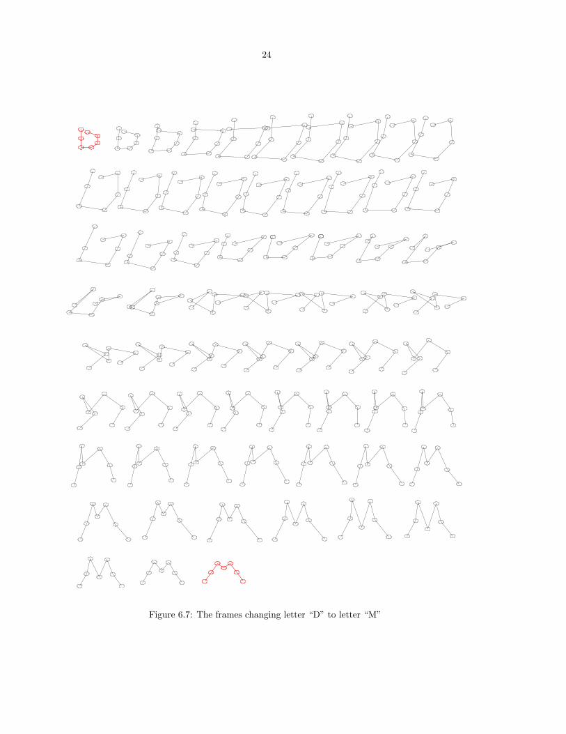
24

Figure 6.7: The frames changing letter “D” to letter “M”

25

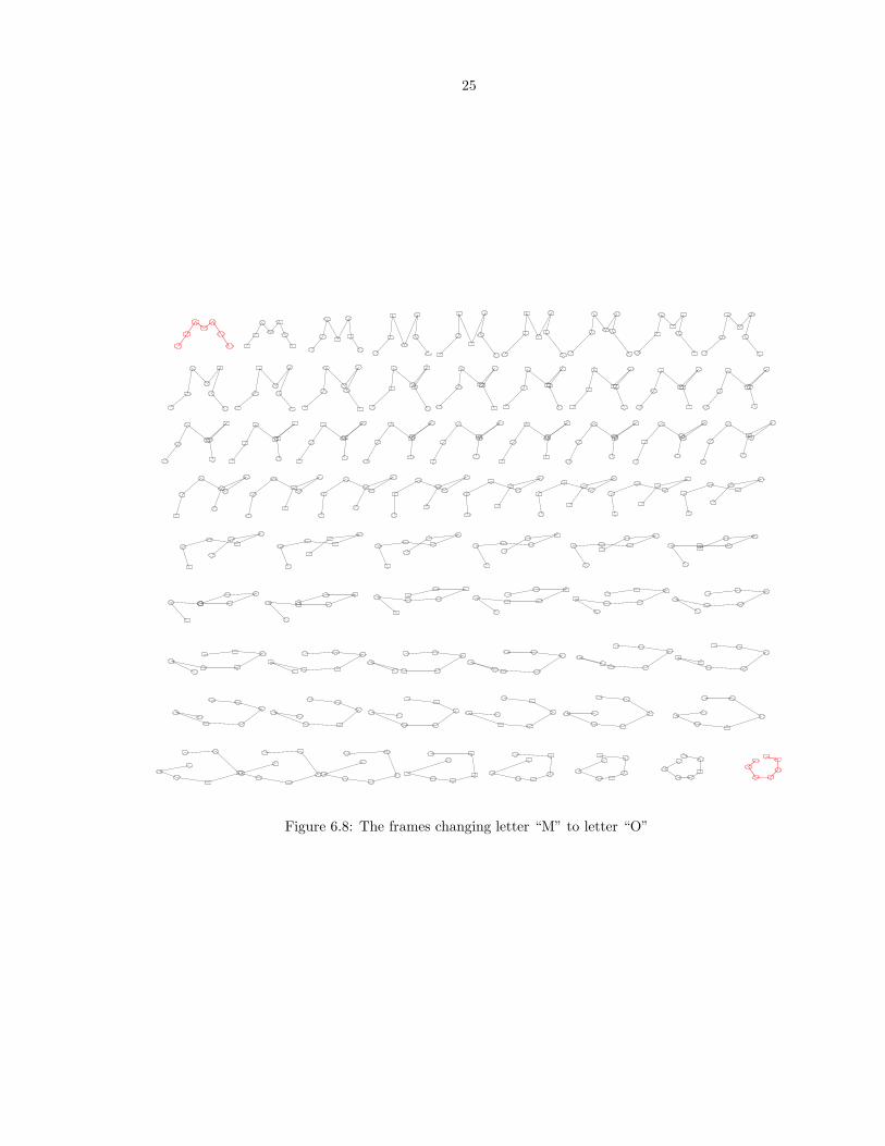
Figure 6.8: The frames changing letter “M” to letter “O”

26

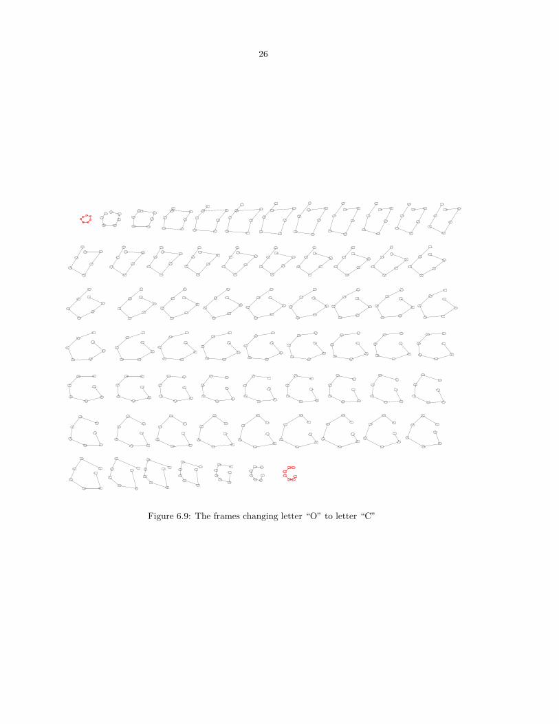
Figure 6.9: The frames changing letter “O” to letter “C”

27

Chapter 7

Discussion about TRACKS

Bergou et al. recently propose a process called TRACKS [4] with similar goals to ours; in their case,

they add physical details, thin shell behavior, to an animation. TRACKS is a three-step process that

first builds a correspondence between guide (coarse input) and tracked (fine output) shapes, then

creates weak-form constraints using Petrov-Galerkin test functions, and finally solves constrained

Lagrangian mechanics equations to add physical details while enforcing the matched constraints.

It was shown to be robust and effective in adding physical details to an existing animation. By

simulating or animating the coarse guide-shapes instead of the fine ones, TRACKS greatly reduces

the computation required, but does not eliminate the hassles of having to manually animate an

entire sequence and having to wrestle with the initial conditions of a simulation.

Our proposed discrete mechanical-interpolation scheme, on the other hand, is less trouble to set

up, requiring only a few input keyframes. However, owing to the number of relaxation steps required,

our method might not be practical for very detailed shapes, which have many degrees of freedom.

If we combine TRACKS and our process, we might be able to reap the benefits of both. Our

discrete mechanical interpolation scheme can be used to generate input animation for coarse-input

guide-shapes; then one can use TRACKS to flesh out the fine physical detailed animation.

28

Chapter 8

Conclusion and Future Work

In this thesis we presented a novel interpolation scheme based on the Lagrange-d’Alembert principle

capable of generating plausible looking motion with physically impossible constraints, along with its

practical implementation and examples using our scheme. Our scheme is similar to DMOC, (discrete

mechanics and optimal control)[11], method used in optimal control, but instead of solving for the

entire motion in one shot, we take a local approach, and solve for a motion one discrete state at

a time using an iterative process. This method can handle systems with much larger degrees of

freedom. It is also excellent in integrating stylistic and artistic choice with the laws of physics to

generate physical looking motion while satisfying conflicting constraints.

For future work, we plan to explore ways to cut down computational time, perhaps by taking a

more DMOC approach by solving for and relaxing multiple states simultaneously, instead of one at

a time. We would also like to adapt our methods to handling interpolation of colliding objects and

systems with discontinuous Lagrangians.

29

Bibliography

[1] David Baraff and Andrew Witkin. Large steps in cloth simulation. In ACM SIGGRAPH, pages

43–54, 1998.

[2] Jernej Barbic and Doug James. Real-Time Subspace Integration for St. Venant-Kirchhoff De-

formable Models. ACM Trans. on Graphics, 24(3):982–990, August 2005.

[3] Steven J. Benson, Lois Curfman McInnes, Jorge More, and Jason Sarich. TAO user manual

(revision 1.7). Technical Report ANL/MCS-TM-242, Argonne National Lab, 2004.

[4] Miklos Bergou, Saurabh Mathur, Max Wardetzky, and Eitan Grinspun. TRACKS: Toward

Directable Thin Shells. SIGGRAPH (ACM Transactions on Graphics), Aug 2007.

[5] J. Bonet and A. Burton. A Simple Average Nodal Pressure Tetrahedral Element for Incom-

pressible and Nearly Incompressible Dynamic Explicit Applications. Comm. in Num. Meth. in

Eng., 14(5):437–449, 1998.

[6] R. C. Fetecau, J. E. Marsden, M. Ortiz, and M. West. Nonsmooth Lagrangian Mechanics and

Variational Collision Integrators. SIAM J. Applied Dynamical Systems, 2(3):381–416, 2003.

[7] Razvan C. Fetecau, Jerrold E. Marsden, Michael Ortiz, and Matt West. Nonsmooth Lagrangian

Mechanics and Variational Collision Integrators. SIAM J. Applied Dynamical Systems, 2:381–

416, 2003.

[8] Ernst Hairer, Christian Lubich, and Gerhard Wanner. Geometric Numerical Integration:

Structure-Preserving Algorithms for ODEs. Springer, 2002.

[9] Michael Hauth, Olaf Etzmuß, and Wolfgang Straßer. Analysis of Numerical Methods for the

Simulation of Deformable Models. The Visual Computer, 19(7-8):581–600, 2003.

[10] H.Yoshimura and J.E.Marsden. Dirac Structures and Lagrangian Mechanics. J. Geom. and

Physics, 2006.

[11] O. Junge, J.E. Marsden, and S. Ober-Blobaum. Discrete Mechanics and Optimal Control. In

Proc. of IFAC World Congress, pages We–M14–TO/3, 2005.

30

[12] Couro Kane, Jerrold E. Marsden, Michael Ortiz, and Matt West. Variational Integrators and

the Newmark Algorithm for Conservative and Dissipative Mechanical Systems. I.J.N.M.E.,

49:1295–1325, 2000.

[13] L. Kharevych, Weiwei, Y. Tong, E. Kanso, J. E. Marsden, P. Schrder, and M. Desbrun. Geo-

metric, Variational Integrators for Computer Animation. ACM/EG Symposium on Computer

Animation, pages 43–51, 2006.

[14] P. Krysl, S. Lall, and J.E. Marsden. Dimensional Model Reduction in Non-linear Finite Element

Dynamics of Solids and Structures. I.J.N.M.E., 51:479–504, 2000.

[15] S.K. Lahiri, J. Bonet, J. Peraire, and L. Casals. A Variationally Consistent Fractional Time

Step Integration Method for Lagrangian Dynamics. Int. J. Numer. Meth. Engng, 3:1–23, 2003.

[16] S. Lall and M. West. Discrete variational Hamiltonian mechanics. J. Phys. A: Math. Gen.,

39:5509–5519, 2006.

[17] Adrian Lew. Variational Time Integrators in Computational Solid Mechanics. PhD thesis,

Caltech, May 2003.

[18] Adrian Lew, Jerrold E. Marsden, Michael Ortiz, and Matt West. Asynchronous Variational

Integrators. Arch. Rational Mech. Anal., 167:85–146, 2003.

[19] J.E. Marsden and M. West. Discrete Mechanics and Variational Integrators. Acta Numerica,

pages 357–515, 2001.

[20] Jorge Nocedal and Stephen J. Wright. Numerical Optimization. Series in Operations Research.

Springer, 1999.

[21] Richard Parent. Computer Animation: Algorithms and Techniques. Morgan Kaufmann, 2001.

[22] William H. Press, Brian P. Flannery, Saul A. Teukolsky, and William T. Vetterling. Numerical

Recipes in C: The Art of Scientific Computing. Cambridge University Press, 2nd edition, 1992.

[23] Raul Radovitzky and Michael Ortiz. Error Estimation and Adaptive Meshing in Strongly

Nonlinear Dynamic Problems. Comput. Method. Appl. M, 172(1-4):203–240, 1999.

[24] Ari Stein and Mathieu Desbrun. Discrete geometric mechanics for variational time integrators.

In Discrete Differential Geometry. ACM SIGGRAPH Course Notes, 2006.

[25] A. Wachter and L. T. Biegler. On the Implementation of a Primal-Dual Interior Point Filter

Line Search Algorithm for Large-Scale Nonlinear Programming. Mathematical Programming

106(1), pages 25–57, 2006.

[26] Matthew West. Variational Integrators. PhD thesis, Caltech, June 2003.