Embed Size (px)
Citation preview
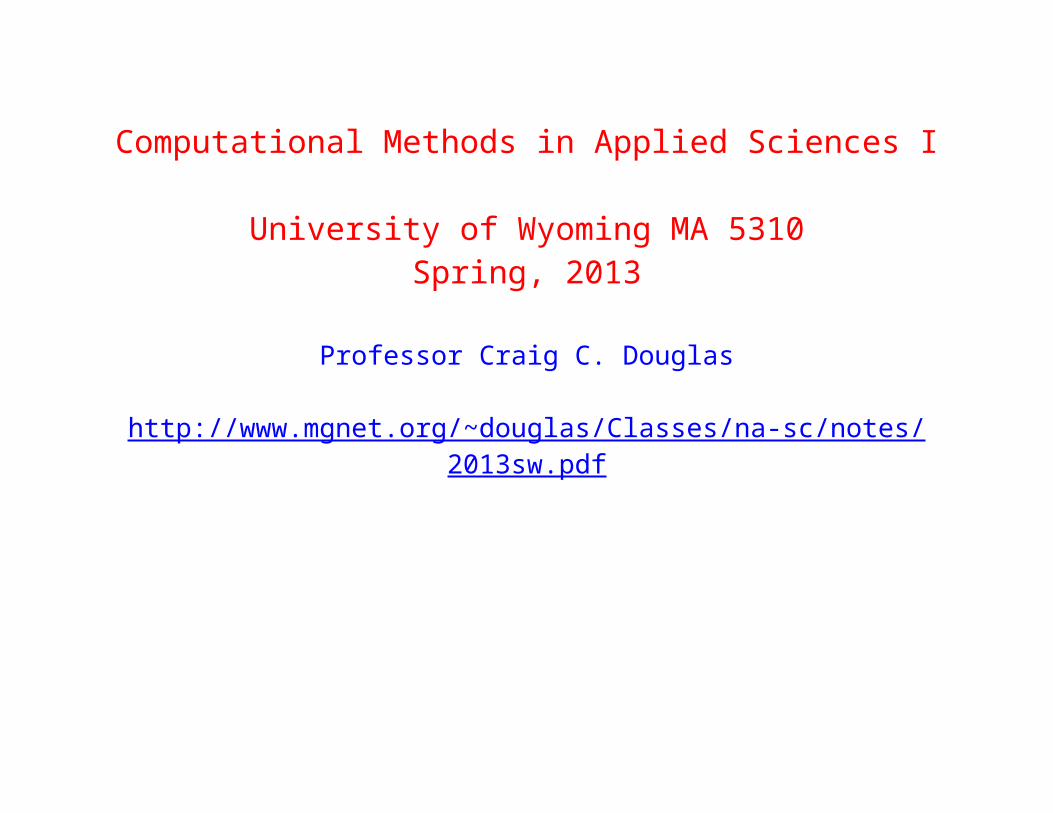
Computational Methods in Applied Sciences I
University of Wyoming MA 5310Spring, 2013
Professor Craig C. Douglas
http://www.mgnet.org/~douglas/Classes/na-sc/notes/2013sw.pdf
Course Description: First semester of a three-semester computational methods series. Review of basics (round off errors and matrix algebra review), finite differences and Taylor expansions, solution of linear systems of equations (Gaussian elimination variations (tridiagonal, general, and sparse matrices), iterative methods (relaxation and conjugate gradient methods), and overdetermined systems (least squares)), nonlinear equations (root finding of functions), interpolation and approximation (polynomial, Lagrange, Hermite, piecewise polynomial, Chebyshev, tensor product methods, and least squares fit), numerical integration (traditional quadrature rules and automatic quadrature rules), and one other topic (simple optimization methods, Monte-Carlo, etc.).(3 hours)Prerequisites: Math 3310 and COSC 1010. Identical to COSC 5310, CHE 5140, ME 5140, and CE 5140.Suggestion: Get a Calculus for a single variable textbook and reread it.
Textbook: George Em Karniadakis and Robert M. Kirby II, Parallel Scientific Computing in C++ and MPI: A Seamless Approach to Parallel Algorithms and Their Implementation, Cambridge University Press, 2003.
2
Preface: Outline of Course
Errors
In pure mathematics, a+b is well defined and exact. In computing, a and b might not even be representable in Floating Point numbers (e.g., 3 is not representable in IEEE floating point and is only approximately 3), which is a finite subset of the Reals. In addition, a+b is subject to roundoff errors, a concept unknown in the Reals. We will study computational and numerical errors in this unit.
See Chapter 2.
C++ and parallel communications
If you do not know simple C++, then you will learn enough to get by in this class. While you will be using MPI (message passing interface), you will be taught how to use another set of routines that will hide MPI from you. The advantages of hiding MPI will be given during the lectures. MPI has an
3
enormous number of routines and great functionality. In fact, its vastness is also a disadvantage for newcomers to parallel computing on cluster machines.
See Appendix A and a web link.
Solution of linear systems of equations Ax=b
We will first review matrix and vector algebra. Then we will study a variety of direct methods (ones with a predictable number of steps) based on Gaussian elimination. Then we will study a collection of iterative methods (ones with a possibly unpredictable number of steps) based on splitting methods. Then we will study Krylov space methods, which are a hybrid of the direct and iterative paradigms. Finally we will study methods for sparse matrices (ones that are almost all zero).
See Chapters 2, 7, and 9.
4
Solution of nonlinear equations
We will develop methods for finding specific values of one variable functions using root finding and fixed point methods.
See Chapters 3 and 4.
Interpolation and approximation
Given {f(x0), f(x1), …, f(xN+1)}, what is f(x), x0xxN+1 and xi<xi+1?
See Chapter 3.
Numerical integration and differentiation
Suppose I give you an impossible to integrate (formally) function f(x) and a domain of integration. How do you approximate the integral? Numerical integration, using quadrature rules, turns out to be relatively simple.
5
Alternately, given a reasonable function g(x), how do I takes its derivative using just a computer? This turns out to be relatively difficult in comparison to integration. Surprisingly, from a numerical viewpoint, it is the exact opposite of what freshman calculus students determine in terms of hardness.
Finally, we will look at simple finite difference methods for approximating ordinary differential equations.
See Chapters 4, 5, and 6.
Specialized topic(s)
If there is sufficient time at the end of the course, one or more other topics will be covered, possibly by the graduate students in the class.
6
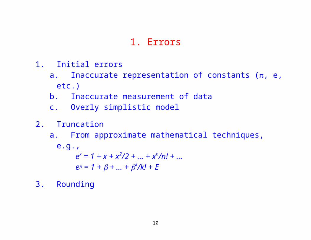
1. Errors
1. Initial errorsa. Inaccurate representation of constants (, e, etc.)b. Inaccurate measurement of datac. Overly simplistic model
2. Truncationa. From approximate mathematical techniques, e.g.,
ex = 1 + x + x2/2 + … + xn/n! + … e = 1 + + … + k/k! + E
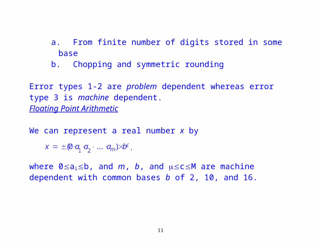
3. Roundinga. From finite number of digits stored in some baseb. Chopping and symmetric rounding
Error types 1-2 are problem dependent whereas error type 3 is machine dependent.Floating Point Arithmetic
7
We can represent a real number x by
where 0aib, and m, b, and cM are machine dependent with common bases b of 2, 10, and 16.
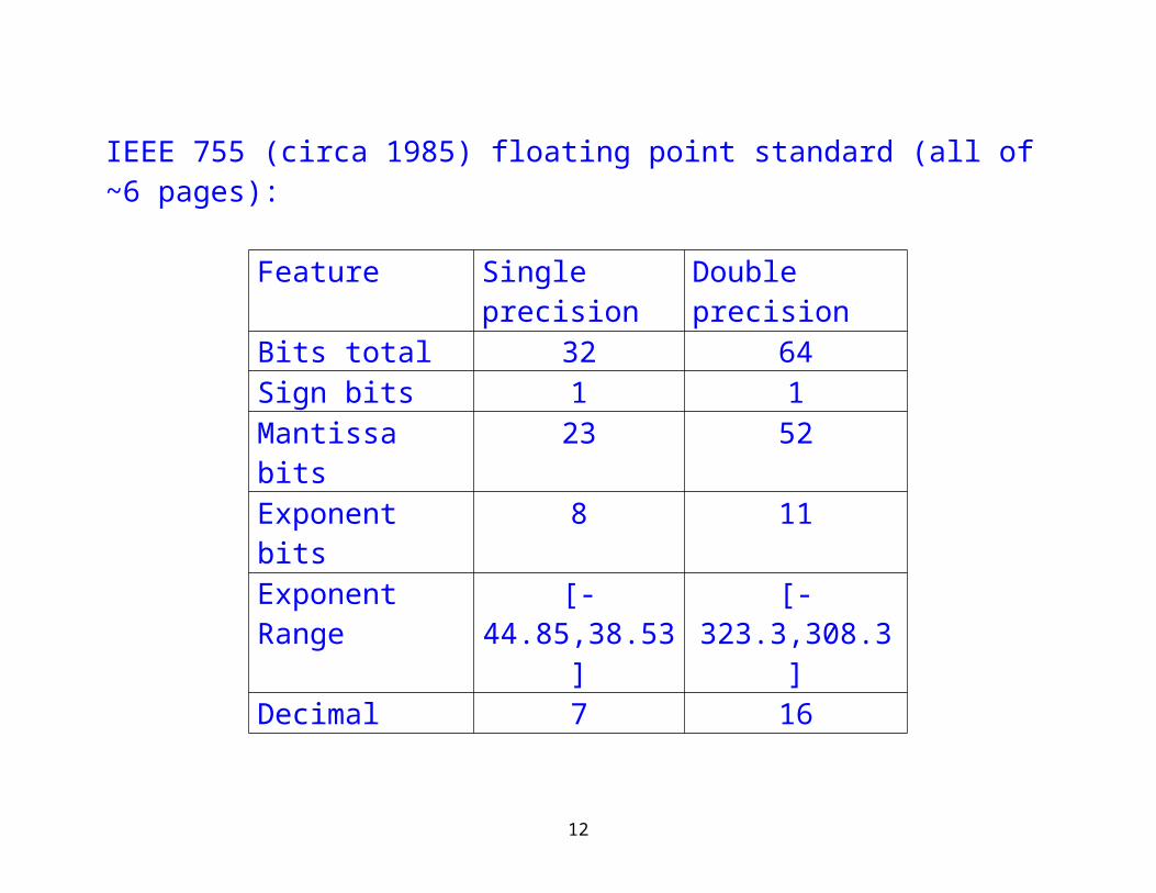
IEEE 755 (circa 1985) floating point standard (all of ~6 pages):
Feature Single precision Double precisionBits total 32 64Sign bits 1 1Mantissa bits 23 52Exponent bits 8 11Exponent Range [-44.85,38.53] [-323.3,308.3]Decimal digits 7 16
8
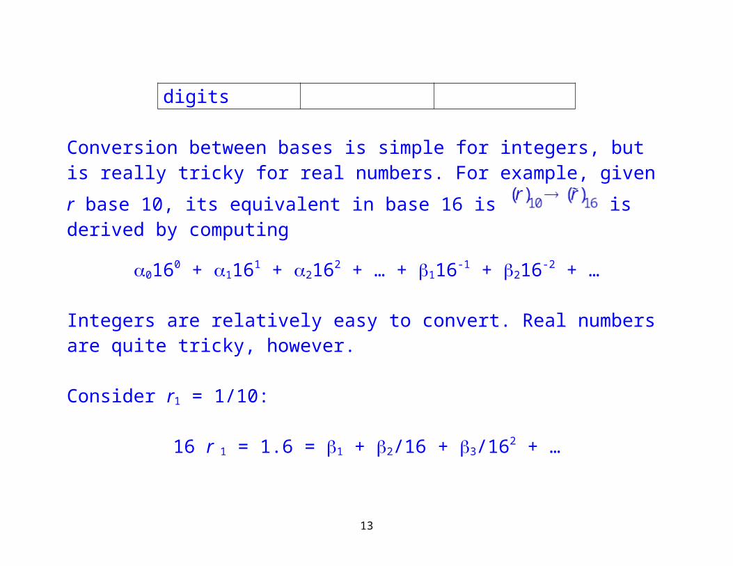
Conversion between bases is simple for integers, but is really tricky for real
numbers. For example, given r base 10, its equivalent in base 16 is is derived by computing
0160 + 1161 + 2162 + … + 116-1 + 216-2 + …
Integers are relatively easy to convert. Real numbers are quite tricky, however.
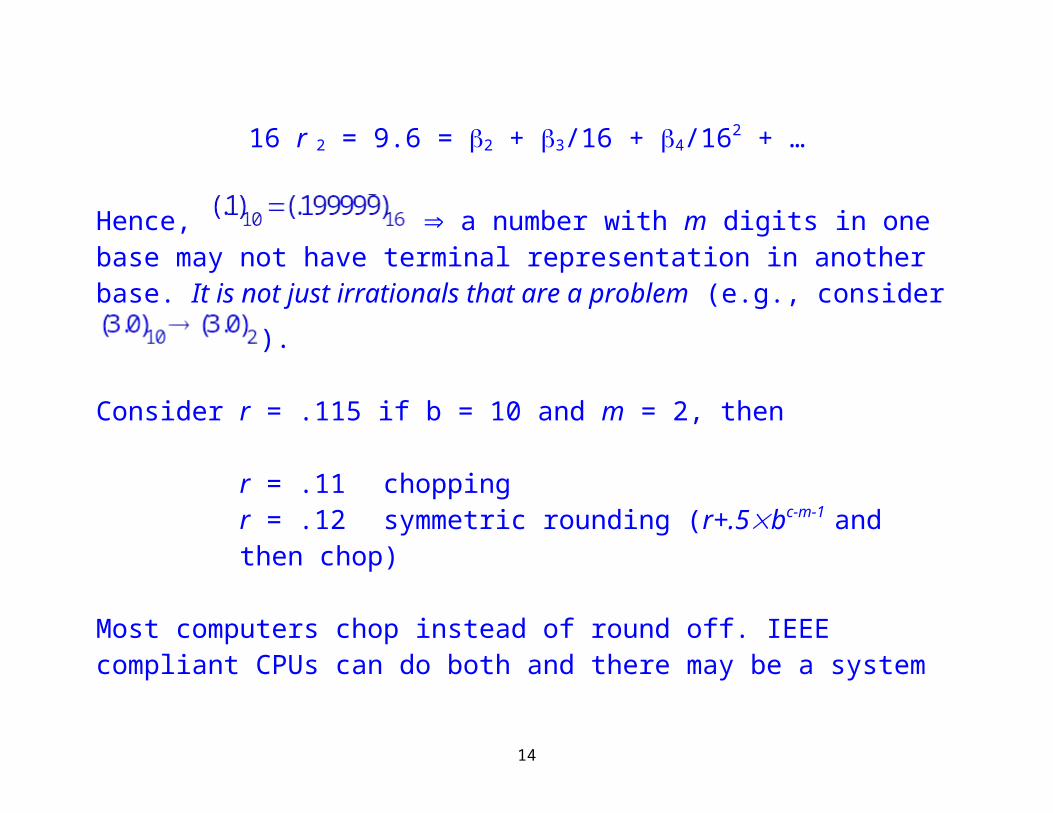
Consider r1 = 1/10:
16 r 1 = 1.6 = 1 + 2/16 + 3/162 + …16 r 2 = 9.6 = 2 + 3/16 + 4/162 + …
Hence, a number with m digits in one base may not have terminal representation in another base. It is not just irrationals that are a
problem (e.g., consider ).
9
Consider r = .115 if b = 10 and m = 2, then
r = .11 choppingr = .12 symmetric rounding (r+.5bc-m-1 and then chop)
Most computers chop instead of round off. IEEE compliant CPUs can do both and there may be a system call to switch, which is usually not user accessible.
Note: When the rounding changes, almost all nontrivial codes break.
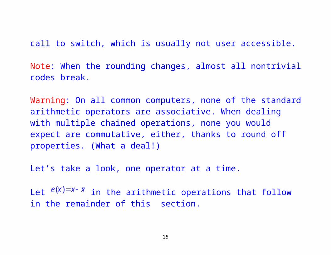
Warning: On all common computers, none of the standard arithmetic operators are associative. When dealing with multiple chained operations, none you would expect are commutative, either, thanks to round off properties. (What a deal!)
Let’s take a look, one operator at a time.
Let in the arithmetic operations that follow in the remainder of this section.
10
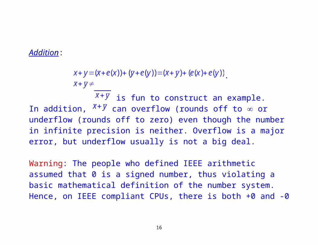
Addition:
.
is fun to construct an example.In addition, can overflow (rounds off to or underflow (rounds off to zero) even though the number in infinite precision is neither. Overflow is a major error, but underflow usually is not a big deal.
Warning: The people who defined IEEE arithmetic assumed that 0 is a signed number, thus violating a basic mathematical definition of the number system. Hence, on IEEE compliant CPUs, there is both +0 and -0 (but no signless 0), which are different numbers in floating point. This seriously disrupts comparisons with 0. The programming fix is to compare abs(expression) with 0, which is computationally ridiculous and inefficient.
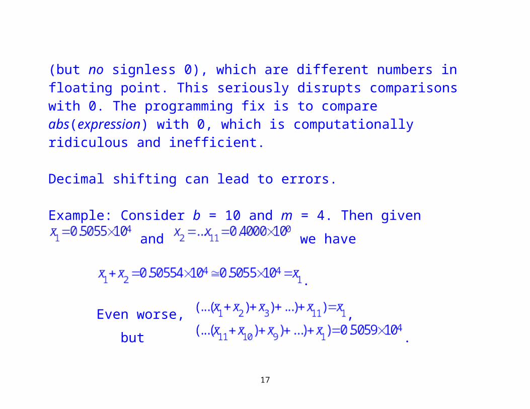
Decimal shifting can lead to errors.
11
Example: Consider b = 10 and m = 4. Then given and
we have
.
Even worse, ,
but .
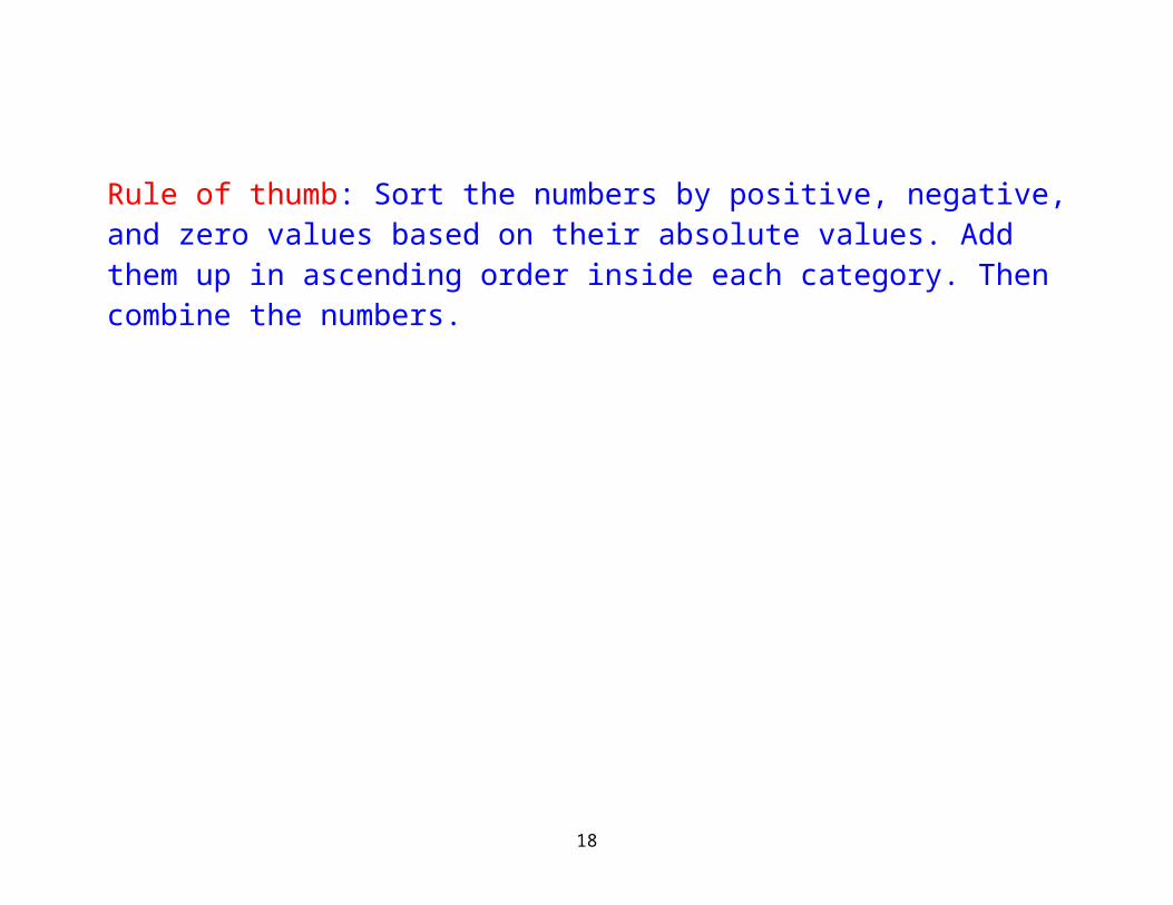
Rule of thumb: Sort the numbers by positive, negative, and zero values based on their absolute values. Add them up in ascending order inside each category. Then combine the numbers.
12
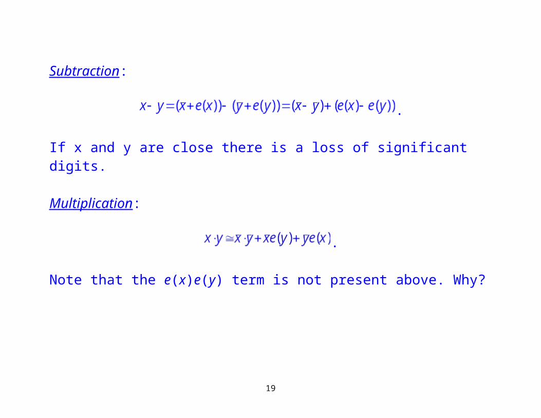
Subtraction:
.
If x and y are close there is a loss of significant digits.
Multiplication:
.
Note that the e(x)e(y) term is not present above. Why?
13
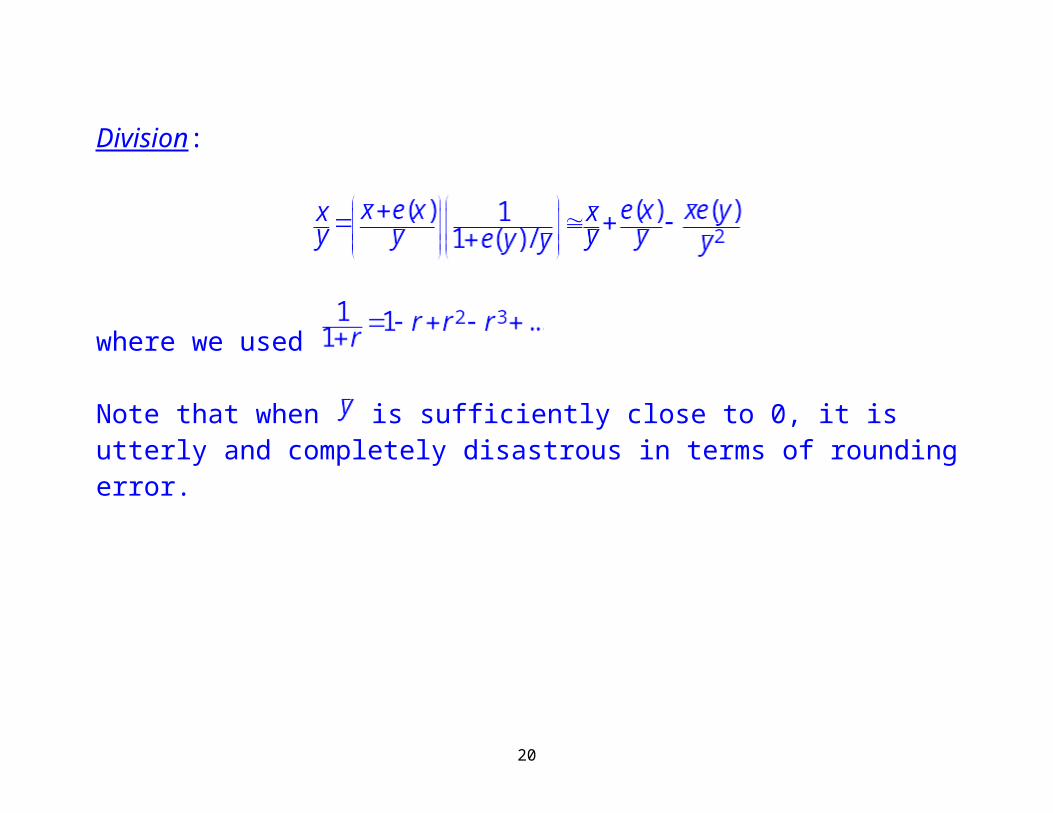
Division:
where we used
Note that when is sufficiently close to 0, it is utterly and completely disastrous in terms of rounding error.
14
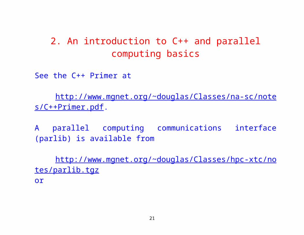
2. An introduction to C++ and parallel computing basics
See the C++ Primer at
http://www.mgnet.org/~douglas/Classes/na-sc/notes/C++Primer.pdf.
A parallel computing communications interface (parlib) is available from
http://www.mgnet.org/~douglas/Classes/hpc-xtc/notes/parlib.tgzor http://www.mgnet.org/~douglas/Classes/hpc-xtc/notes/parlib.zip
with documentation available from
http://www.mgnet.org/~douglas/Classes/hpc-xtc/notes/parlib.pdf.
15
Assume there are p processors numbered from 0 to p-1 and labeled Pi. The communication between the processors uses one or more high speed and bandwidth switches.
In the old days, various topologies were used, none of which scaled to more than a modest number of processors. The Internet model saved parallel computing.
Today parallel computers come in several flavors (hybrids, too): Small shared memory (SMPs) Small clusters of PCs Blade servers (in one or more racks) Forests of racks GRID or Cloud computing
Google operates the world’s largest Cloud/GRID system. The Top 500 list provides an ongoing list of the fastest computers willing to be measured. It is not a comprehensive list and Google, Yahoo!, and many governments and companies do not participate.
16
Data needs to be distributed sensibly among the p processors. Where the data needs to be can change, depending on the operation, and communication is usual.
Algorithms that essentially never need to communicate are known as embarrassingly parallel. These algorithms scale wonderfully and are frequently used as examples of how well so and so’s parallel system scales. Most applications are not in this category, unfortunately.
To do parallel programming, you need only a few functions to get by: Initialize the environment and find out processor numbers i. Finalize or end parallel processing on one or all processors. Send data to one, a set, or all processors. Receive data from one, a set, or all processors. Cooperative operations on all processors (e.g., sum of a distributed vector).
17
Everything else is a bonus. Almost all of MPI is designed for compiler writers and operating systems developers. Only a small subset is expected to be used by regular people.
18
3. Solution of Linear Systems of Equations
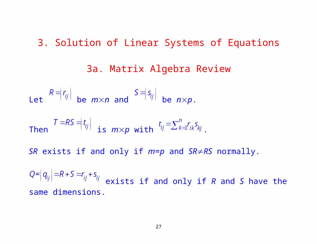
3a. Matrix Algebra Review
Let be mn and be np.
Then is mp with .
SR exists if and only if m=p and SRRS normally.
exists if and only if R and S have the same dimensions.
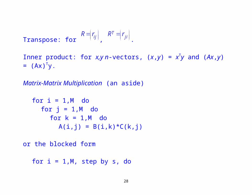
Transpose: for , .
19
Inner product: for x,y n-vectors, (x,y) = xTy and (Ax,y) = (Ax)Ty.
Matrix-Matrix Multiplication (an aside)
for i = 1,M do
for j = 1,M do
for k = 1,M do
A(i,j) = B(i,k)*C(k,j)
or the blocked form
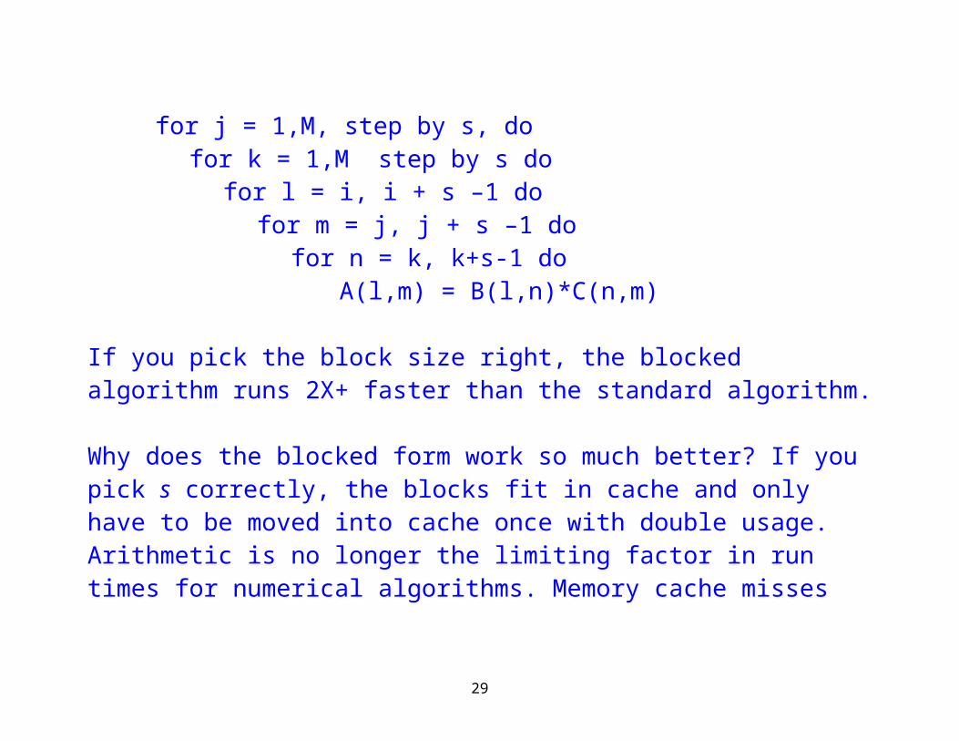
for i = 1,M, step by s, do
for j = 1,M, step by s, do
for k = 1,M step by s do
for l = i, i + s –1 do
for m = j, j + s –1 do
for n = k, k+s-1 do
A(l,m) = B(l,n)*C(n,m)
20
If you pick the block size right, the blocked algorithm runs 2X+ faster than the standard algorithm.
Why does the blocked form work so much better? If you pick s correctly, the blocks fit in cache and only have to be moved into cache once with double usage. Arithmetic is no longer the limiting factor in run times for numerical algorithms. Memory cache misses control the run times and are notoriously hard to model or repeat in successive runs.
An even better way of multiplying matrices is a Strassen style algorithm (the Winograd variant is the fastest in practical usage). A good implementation is the GEMMW code (see http://www.mgnet.org/~douglas/ccd-free-software.html).
21
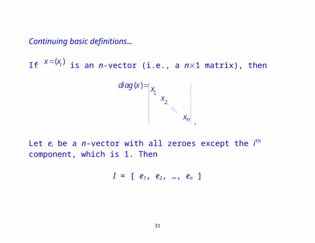
Continuing basic definitions…
If is an n-vector (i.e., a n1 matrix), then
.
Let ei be a n-vector with all zeroes except the ith component, which is 1. Then
I = [ e1, e2, …, en ]
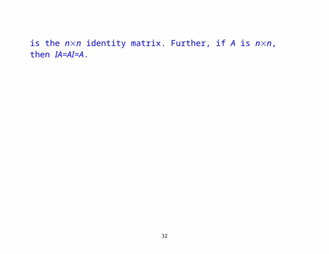
is the nn identity matrix. Further, if A is nn, then IA=AI=A.
22
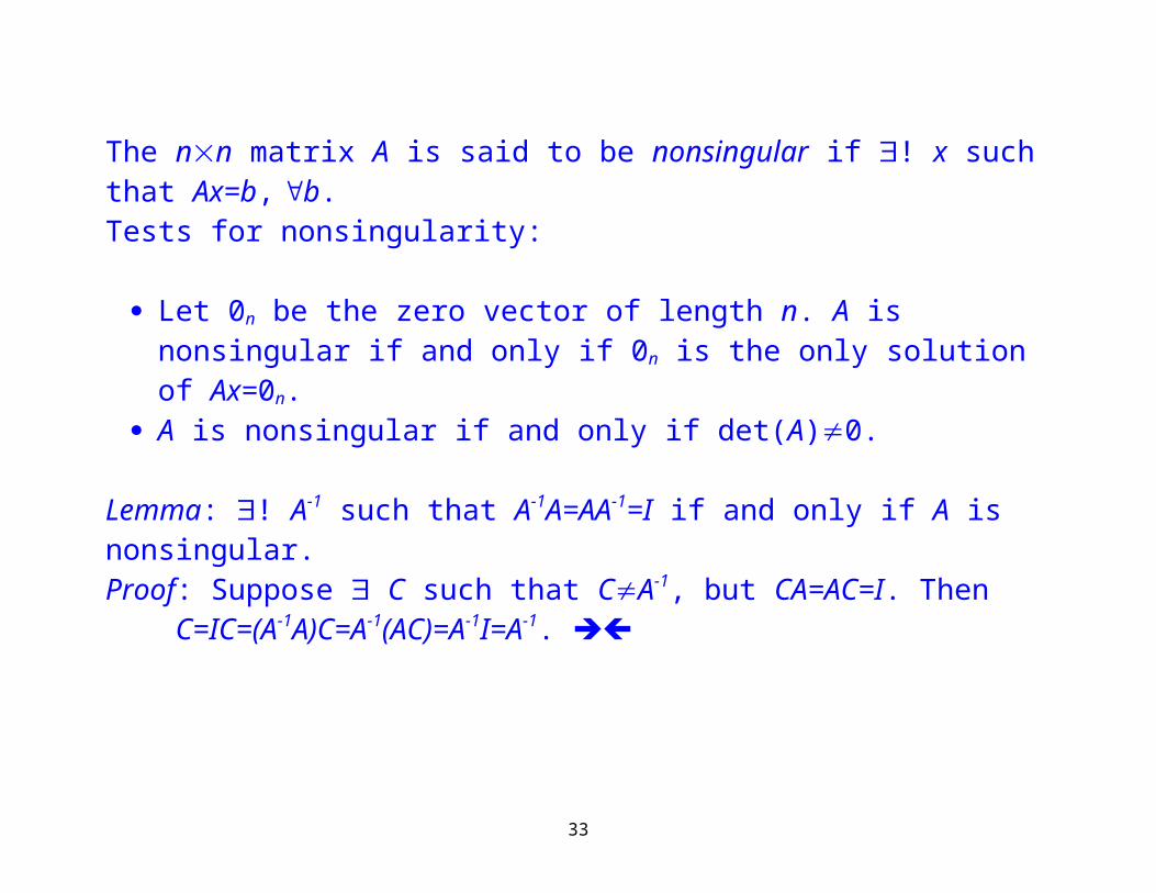
The nn matrix A is said to be nonsingular if ! x such that Ax=b, b.Tests for nonsingularity:
Let 0n be the zero vector of length n. A is nonsingular if and only if 0n is the only solution of Ax=0n.
A is nonsingular if and only if det(A)0.
Lemma: ! A-1 such that A-1A=AA-1=I if and only if A is nonsingular.Proof: Suppose C such that CA-1, but CA=AC=I. Then C=IC=(A-1A)C=A-1(AC)=A-1I=A-1.
23
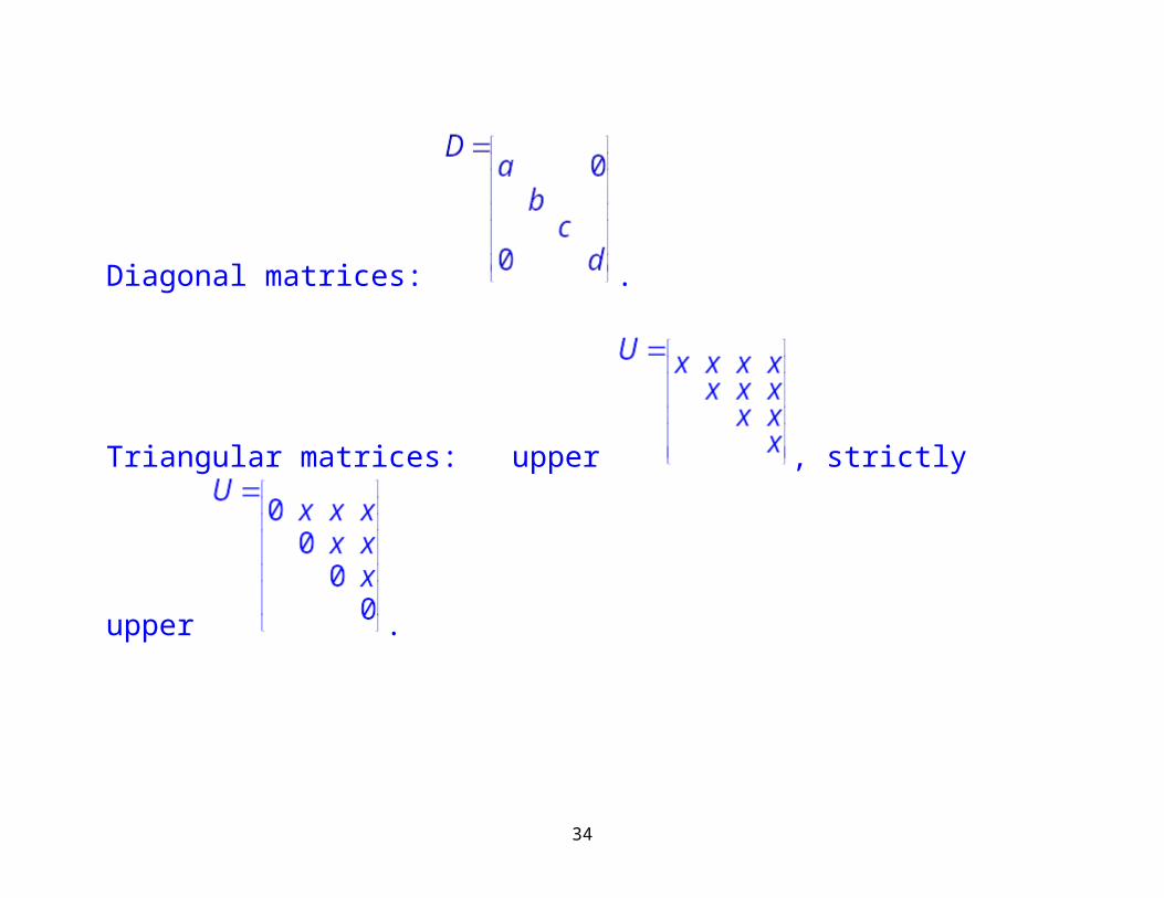
Diagonal matrices: .
Triangular matrices: upper , strictly upper .
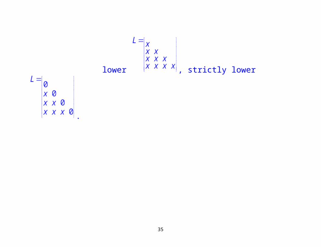
lower , strictly lower .
24
25
3b. Gaussian elimination
Solve Ux=b, U upper triangular, real, and nonsingular:
If we define , then the formal algorithm is
, i=n,n-1, …, 1.
Solve Lx=b, L lower triangular, real, and nonsingular similarly.
Operation count: O(n2) multiplies
26
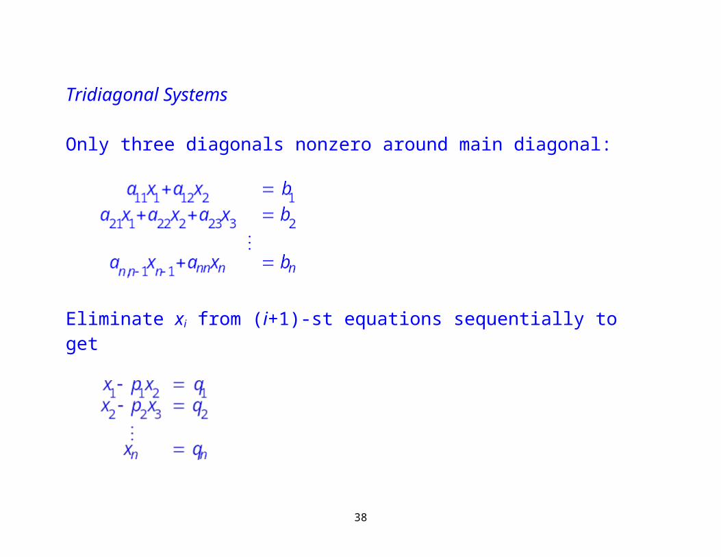
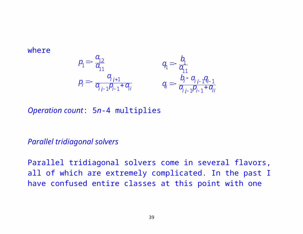
Tridiagonal Systems
Only three diagonals nonzero around main diagonal:
Eliminate xi from (i+1)-st equations sequentially to get
where
27
Operation count: 5n-4 multiplies
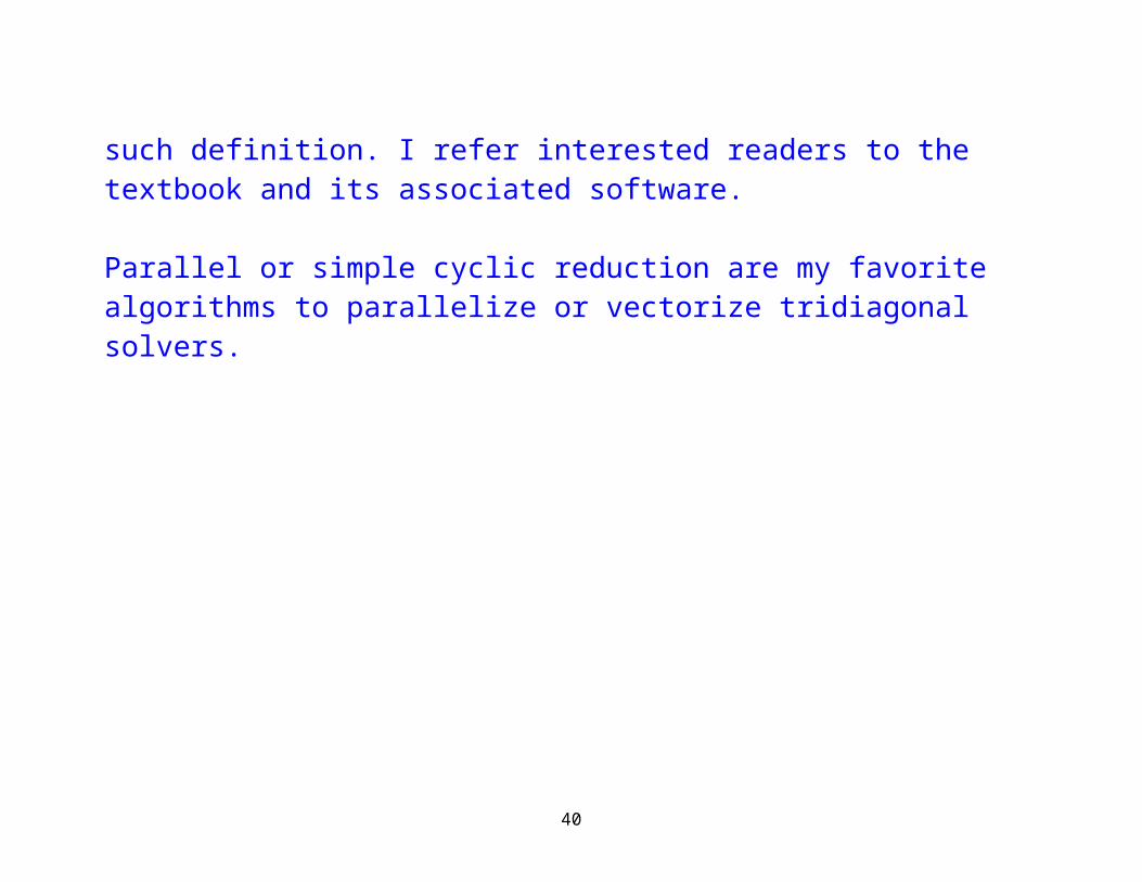
Parallel tridiagonal solvers
Parallel tridiagonal solvers come in several flavors, all of which are extremely complicated. In the past I have confused entire classes at this point with one such definition. I refer interested readers to the textbook and its associated software.
Parallel or simple cyclic reduction are my favorite algorithms to parallelize or vectorize tridiagonal solvers.
28
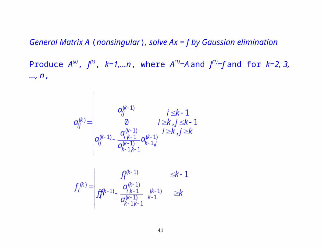
General Matrix A (nonsingular), solve Ax = f by Gaussian elimination
Produce A(k), f(k), k=1,…n, where A(1)=A and f(1)=f and for k=2, 3, …, n,
29
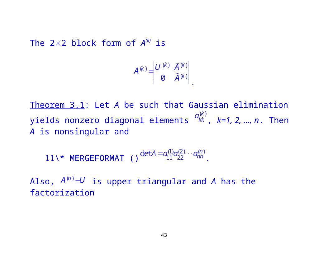
The 22 block form of A(k) is
.
Theorem 3.1: Let A be such that Gaussian elimination yields nonzero diagonal
elements , k=1, 2, …, n. Then A is nonsingular and
11\* MERGEFORMAT () .
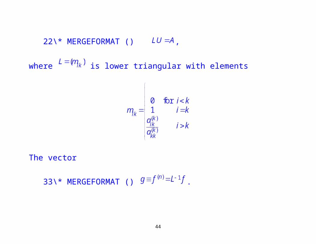
Also, is upper triangular and A has the factorization
22\* MERGEFORMAT () ,
where is lower triangular with elements
30
The vector
33\* MERGEFORMAT () .
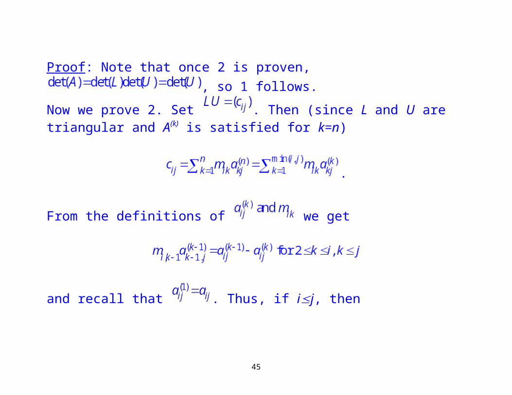
Proof: Note that once 2 is proven, , so 1 follows.
Now we prove 2. Set . Then (since L and U are triangular and A(k) is satisfied for k=n)
.
31
From the definitions of we get
and recall that . Thus, if ij, then
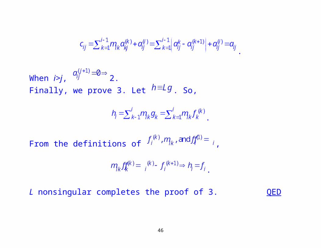
.
When i>j, 2.Finally, we prove 3. Let . So,
.
32
From the definitions of ,
.
L nonsingular completes the proof of 3. QED
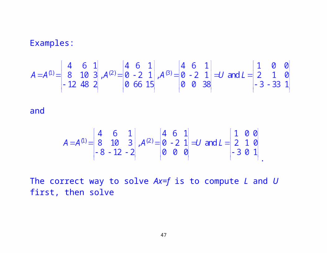
Examples:
and
33
.
The correct way to solve Ax=f is to compute L and U first, then solve
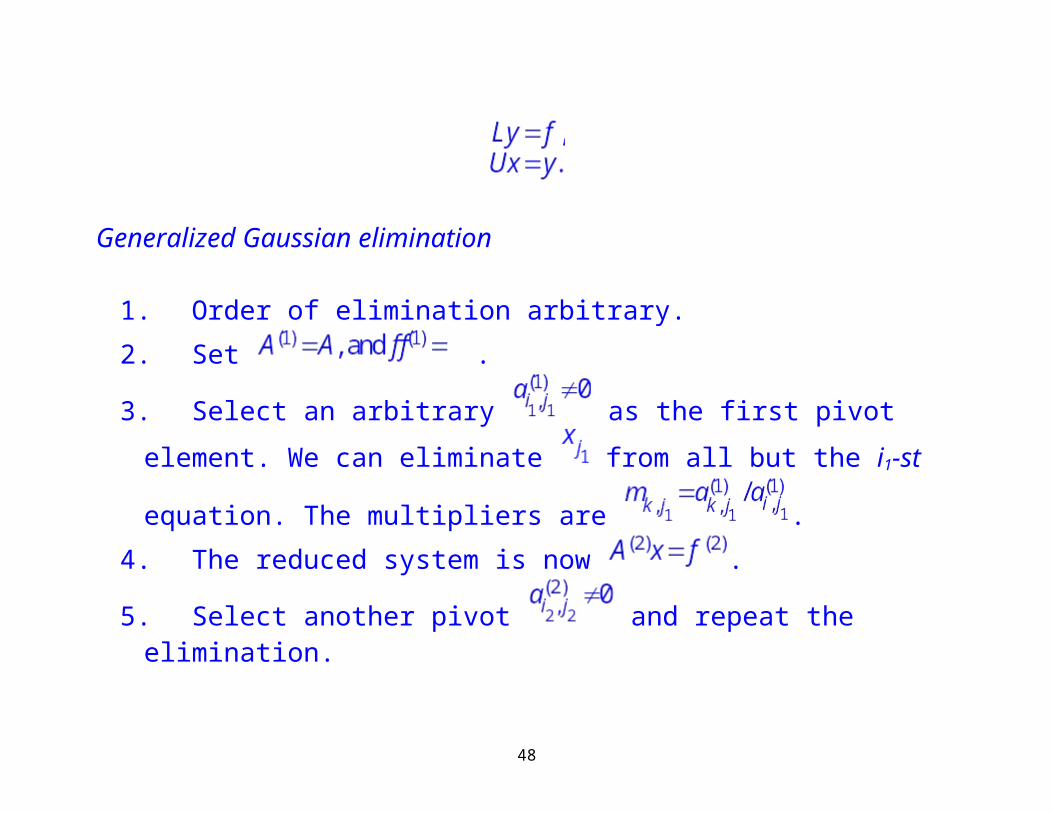
Generalized Gaussian elimination
1. Order of elimination arbitrary.2. Set .
3. Select an arbitrary as the first pivot element. We can eliminate
from all but the i1-st equation. The multipliers are .
34
4. The reduced system is now .
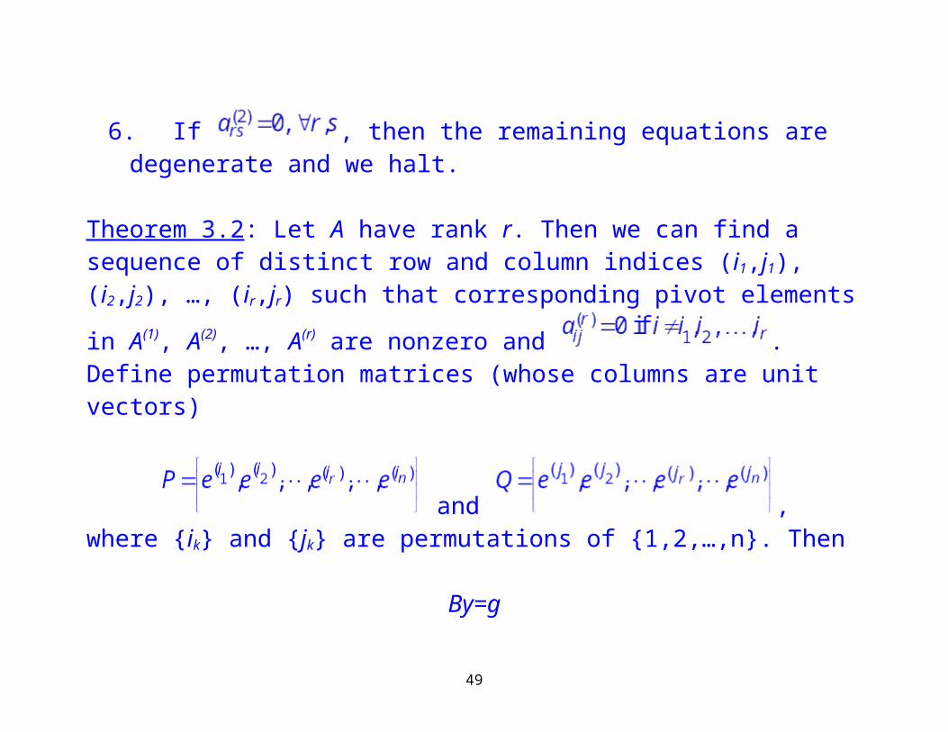
5. Select another pivot and repeat the elimination.6. If , then the remaining equations are degenerate and we halt.
Theorem 3.2: Let A have rank r. Then we can find a sequence of distinct row and column indices (i1,j1), (i2,j2), …, (ir,jr) such that corresponding pivot
elements in A(1), A(2), …, A(r) are nonzero and . Define permutation matrices (whose columns are unit vectors)
and ,where {ik} and {jk} are permutations of {1,2,…,n}. Then
By=g
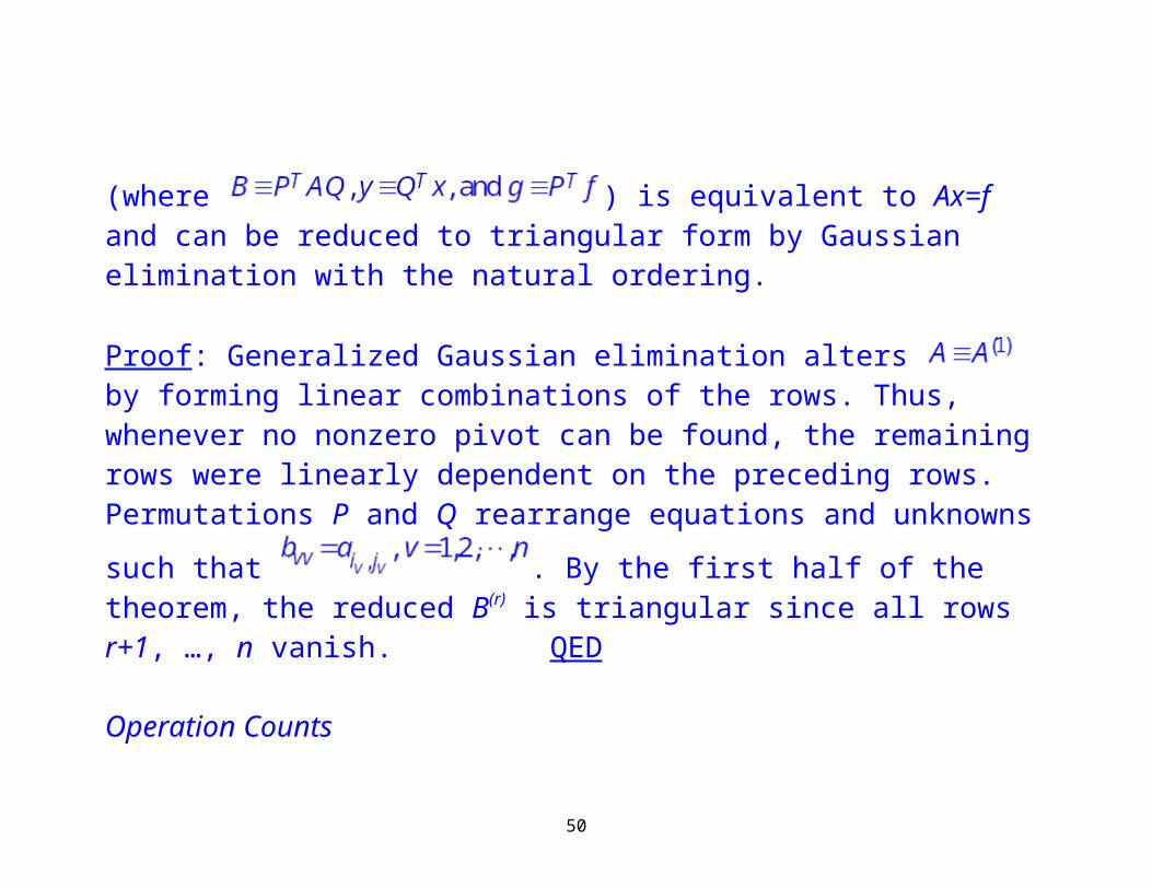
35

(where ) is equivalent to Ax=f and can be reduced to triangular form by Gaussian elimination with the natural ordering.
Proof: Generalized Gaussian elimination alters by forming linear combinations of the rows. Thus, whenever no nonzero pivot can be found, the remaining rows were linearly dependent on the preceding rows. Permutations P
and Q rearrange equations and unknowns such that . By the first half of the theorem, the reduced B(r) is triangular since all rows r+1, …, n vanish. QED
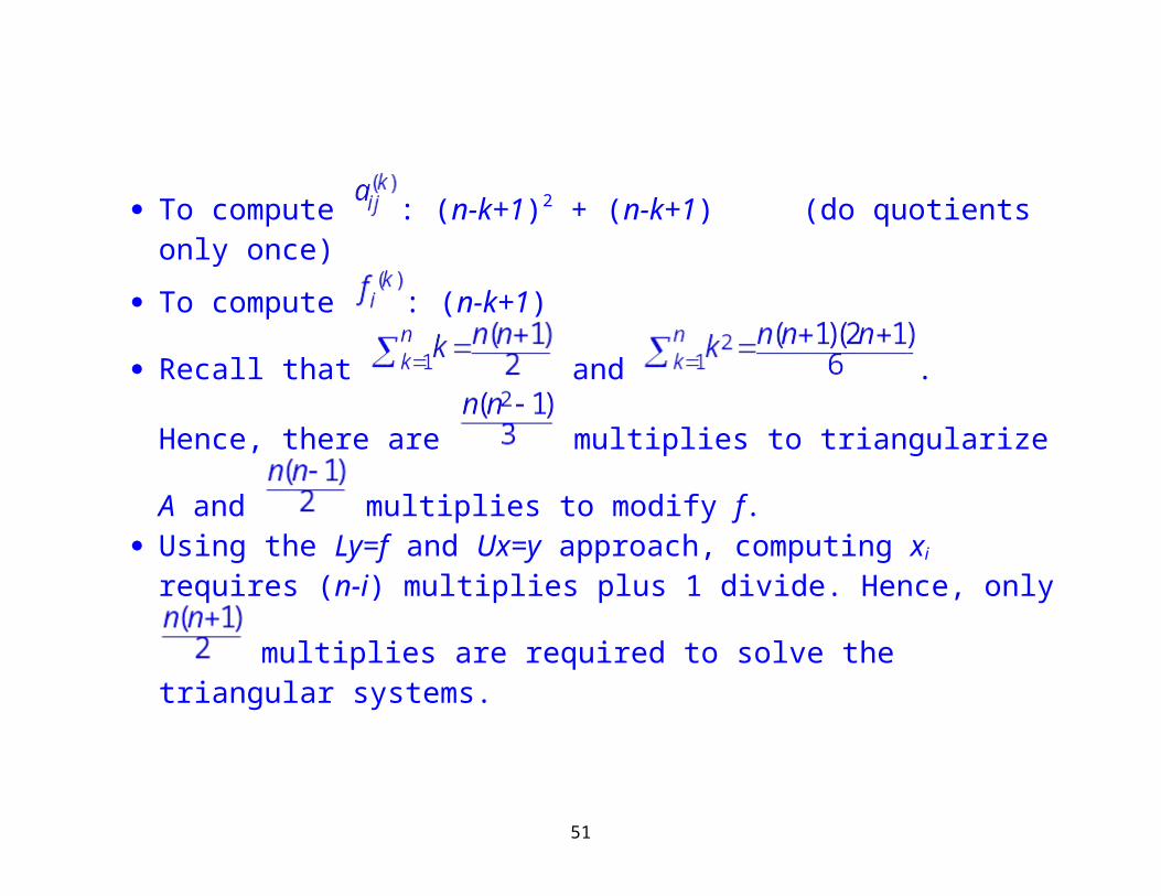
Operation Counts
To compute : (n-k+1)2 + (n-k+1) (do quotients only once)
To compute : (n-k+1)
36
Recall that and . Hence, there are
multiplies to triangularize A and multiplies to modify f. Using the Ly=f and Ux=y approach, computing xi requires (n-i) multiplies
plus 1 divide. Hence, only multiplies are required to solve the triangular systems.
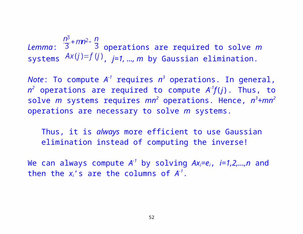
Lemma: operations are required to solve m systems , j=1, …, m by Gaussian elimination.
Note: To compute A-1 requires n3 operations. In general, n2 operations are required to compute A-1f(j). Thus, to solve m systems requires mn2 operations. Hence, n3+mn2 operations are necessary to solve m systems.
37
Thus, it is always more efficient to use Gaussian elimination instead of computing the inverse!
We can always compute A-1 by solving Axi=ei, i=1,2,…,n and then the xi’s are the columns of A-1.
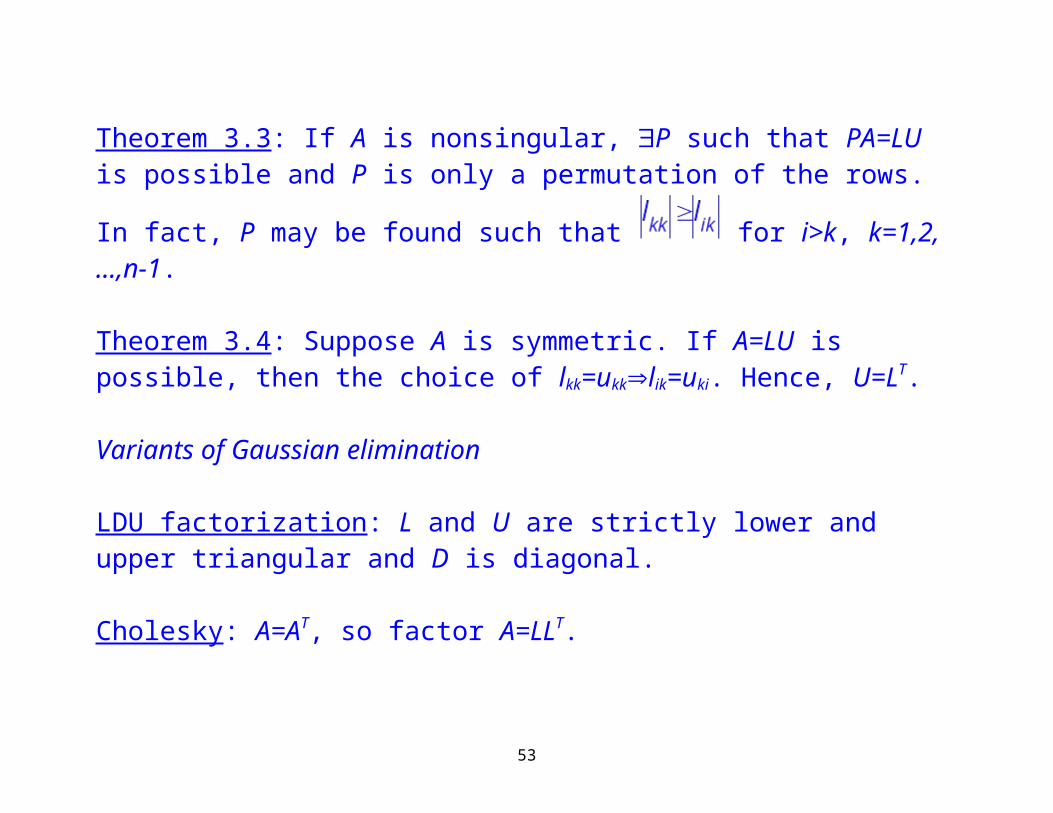
Theorem 3.3: If A is nonsingular, P such that PA=LU is possible and P is only
a permutation of the rows. In fact, P may be found such that for i>k, k=1,2,…,n-1.
Theorem 3.4: Suppose A is symmetric. If A=LU is possible, then the choice of lkk=ukklik=uki. Hence, U=LT.
Variants of Gaussian elimination
LDU factorization: L and U are strictly lower and upper triangular and D is diagonal.
38
Cholesky: A=AT, so factor A=LLT.
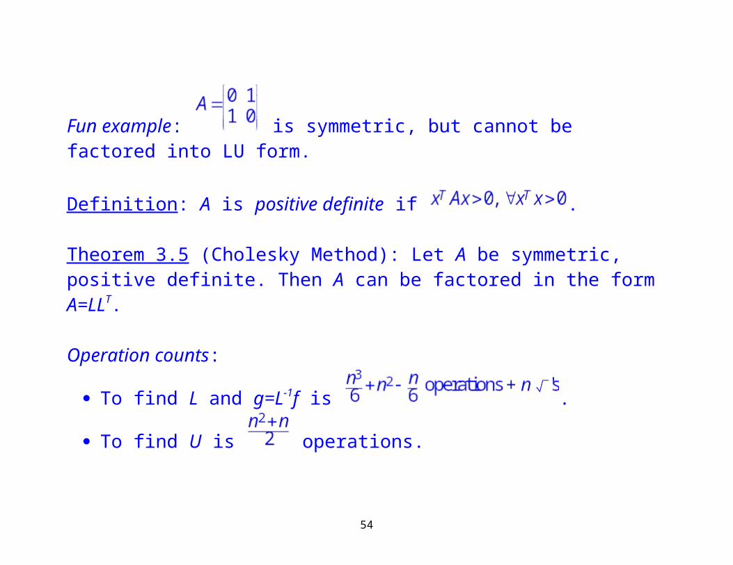
Fun example: is symmetric, but cannot be factored into LU form.
Definition: A is positive definite if .
Theorem 3.5 (Cholesky Method): Let A be symmetric, positive definite. Then A can be factored in the form A=LLT.
Operation counts:
To find L and g=L-1f is .
To find U is operations.
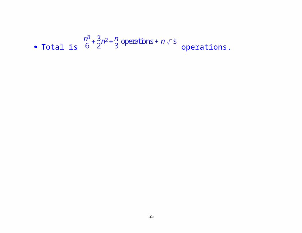
Total is operations.
39
40
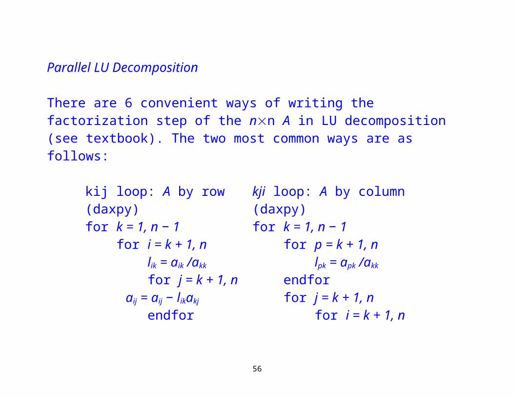
Parallel LU Decomposition
There are 6 convenient ways of writing the factorization step of the nn A in LU decomposition (see textbook). The two most common ways are as follows:
kij loop: A by row (daxpy) kji loop: A by column (daxpy)for k = 1, n − 1 for k = 1, n − 1 for i = k + 1, n for p = k + 1, n lik = aik /akk lpk = apk /akk
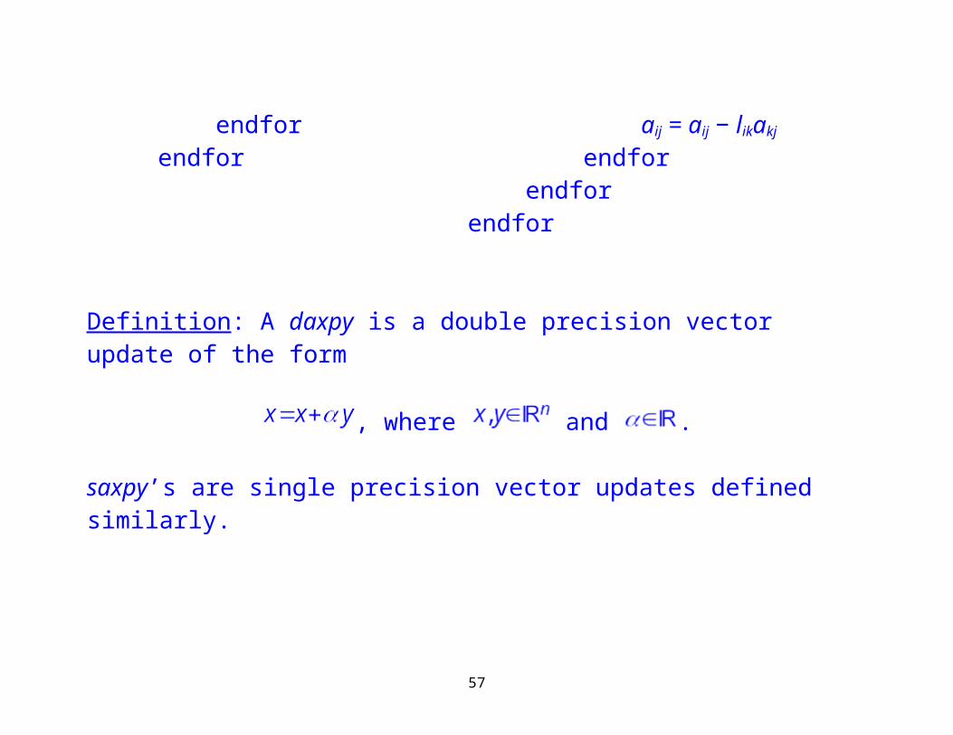
for j = k + 1, n endfor aij = aij − likakj for j = k + 1, n endfor for i = k + 1, n endfor aij = aij − likakj
endfor endfor endforendfor
41

Definition: A daxpy is a double precision vector update of the form
, where and .
saxpy’s are single precision vector updates defined similarly.
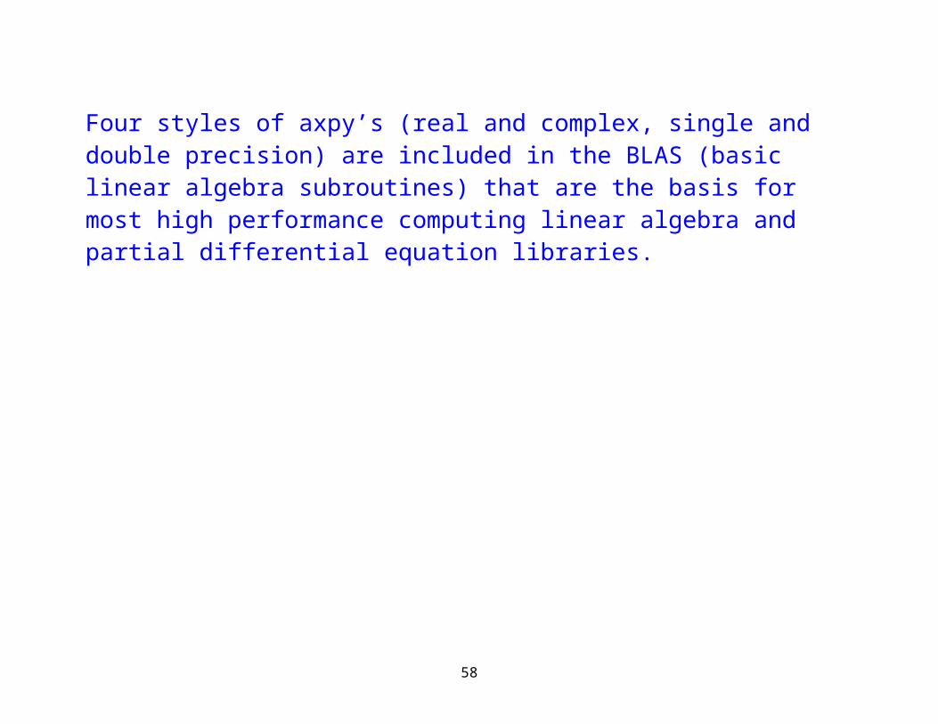
Four styles of axpy’s (real and complex, single and double precision) are included in the BLAS (basic linear algebra subroutines) that are the basis for most high performance computing linear algebra and partial differential equation libraries.
42
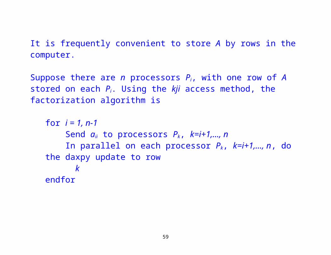
It is frequently convenient to store A by rows in the computer.
Suppose there are n processors Pi, with one row of A stored on each Pi. Using the kji access method, the factorization algorithm is
for i = 1, n-1 Send aii to processors Pk, k=i+1,…, n In parallel on each processor Pk, k=i+1,…, n, do the daxpy update to row kendfor
Note that in step i, after Pi sends aii to other processors that the first i processors are idle for the rest of the calculation. This is highly inefficient if this is the only thing the parallel computer is doing.
A column oriented version is very similar.
43
We can overlap communication with computing to hide some of the expenses of communication. This still does not address the processor dropout issue. We can do a lot better yet.Improvements to aid parallel efficiency:
1. Store multiple rows (columns) on a processor. This assumes that there are p processors and that . While helpful to have mod(n,p)=0, it is unnecessary (it just complicates the implementation slightly).
2. Store multiple blocks of rows (columns) on a processor.3. Store either 1 or 2 using a cyclic scheme (e.g., store rows 1 and 3 on P1 and
rows 2 and 4 on P2 when p=2 and n=4).
Improvement 3, while extremely nasty to program (and already has been as part of Scalapack so you do not have to reinvent the wheel if you choose not to) leads to the best use of all of the processors. No processor drops out. Figuring out how to get the right part of A to the right processors is lots of fun, too, but is also provided in the BLACS, which are required by Scalapack.
44
Now that we know how to factor A = LU in parallel, we need to know how to do back substitution in parallel. This is a classic divide and conquer algorithm leading to an operation count that cannot be realized on a known computer (why?).
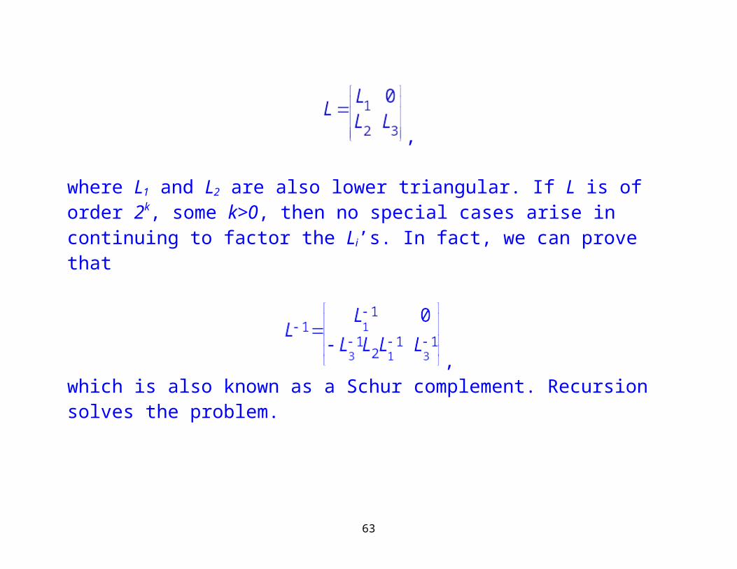
We can write the lower triangular matrix L in block form as
,
where L1 and L2 are also lower triangular. If L is of order 2k, some k>0, then no special cases arise in continuing to factor the Li’s. In fact, we can prove that
,which is also known as a Schur complement. Recursion solves the problem.
45
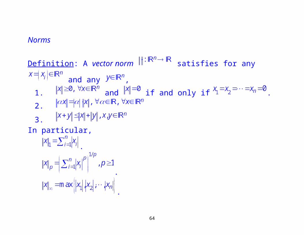
Norms
Definition: A vector norm satisfies for any and any ,
1. and if and only if .
2.
3.In particular,
.
.
.
46
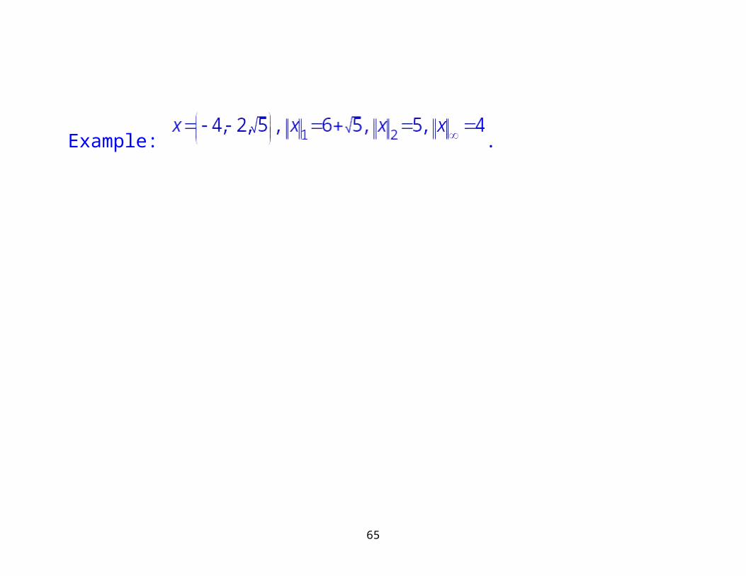
Example: .
47
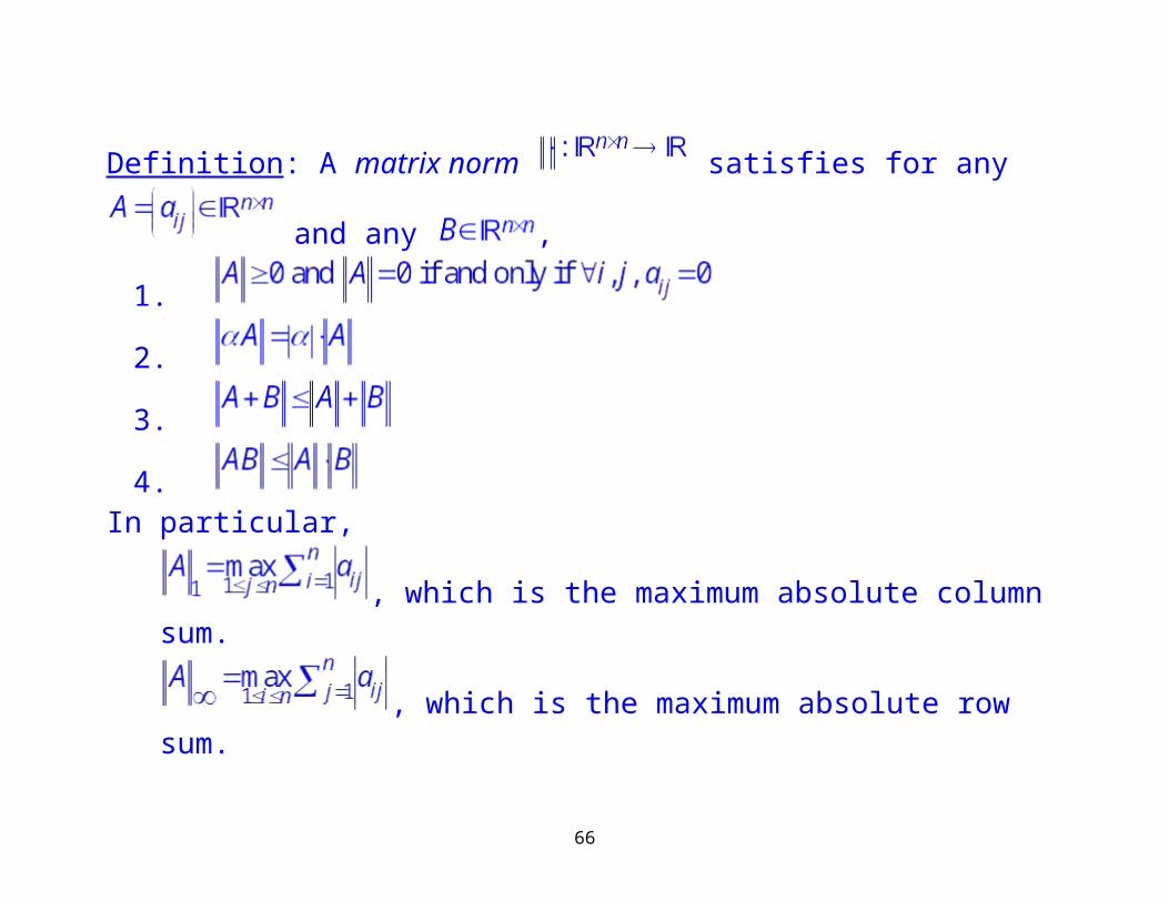
Definition: A matrix norm satisfies for any and any ,
1.
2.
3.
4.In particular,
, which is the maximum absolute column sum.
, which is the maximum absolute row sum.
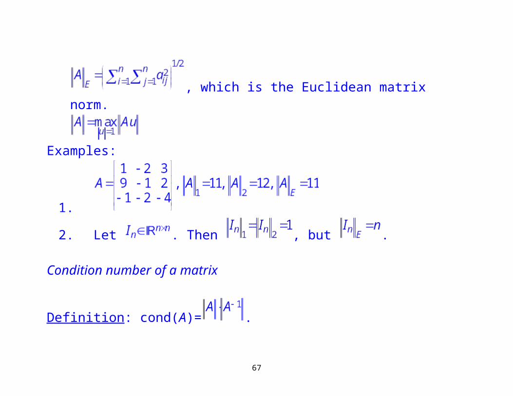
, which is the Euclidean matrix norm.
48
Examples:
1.
2. Let . Then , but .
Condition number of a matrix
Definition: cond(A)= .
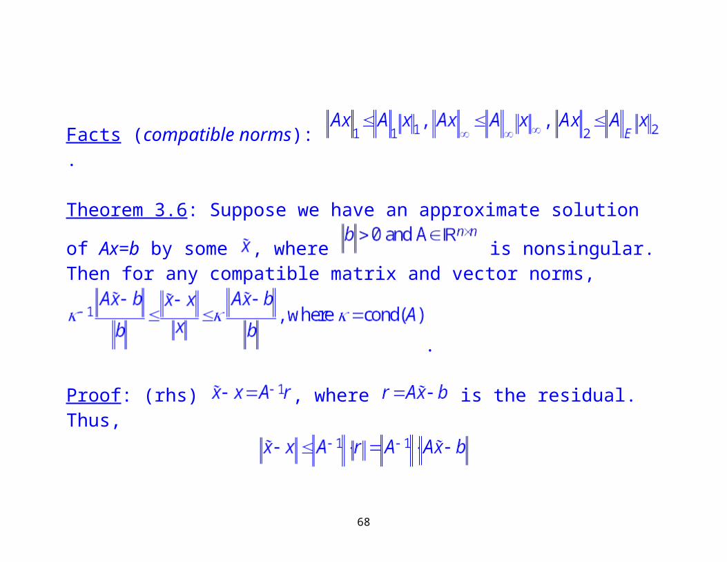
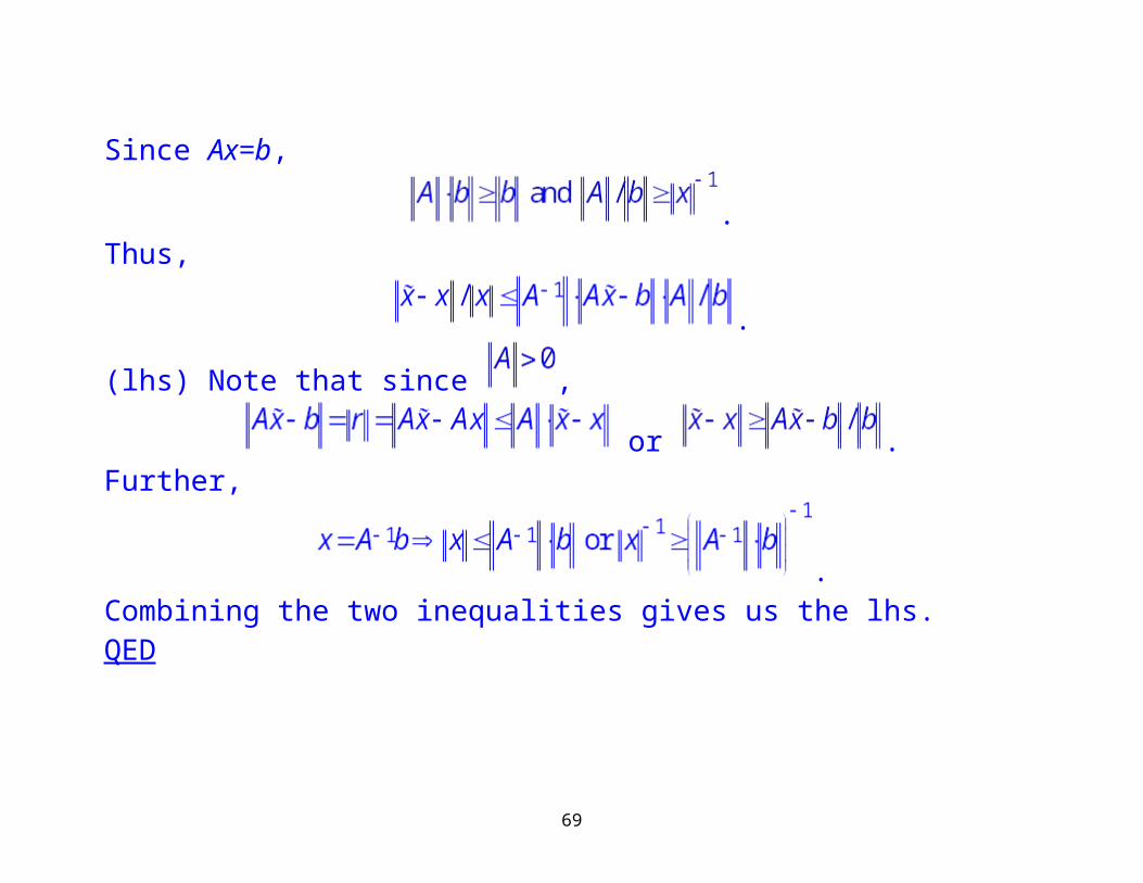
Facts (compatible norms): .
49
Theorem 3.6: Suppose we have an approximate solution of Ax=b by some ,
where is nonsingular. Then for any compatible matrix and
vector norms, .
Proof: (rhs) , where is the residual. Thus,
Since Ax=b,
.Thus,
.
(lhs) Note that since ,
50
or .Further,
.Combining the two inequalities gives us the lhs. QED
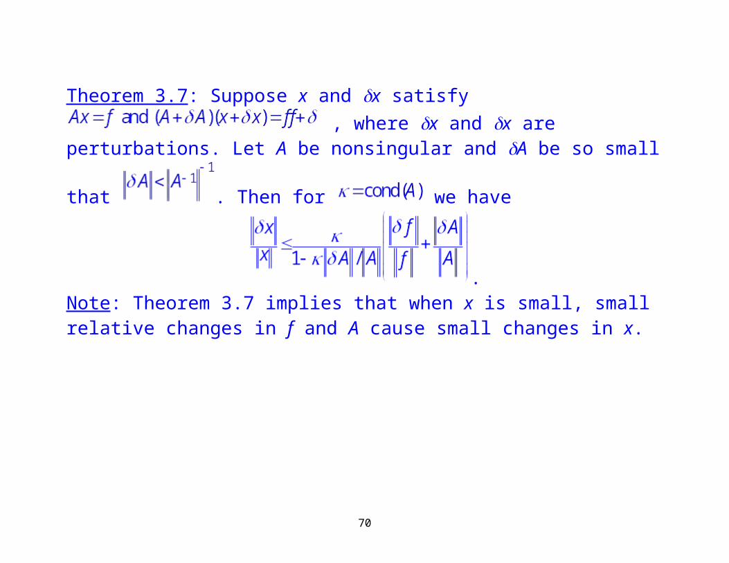
Theorem 3.7: Suppose x and x satisfy , where x and x are perturbations. Let A be nonsingular and A be so small that
. Then for we have
.Note: Theorem 3.7 implies that when x is small, small relative changes in f and A cause small changes in x.
51
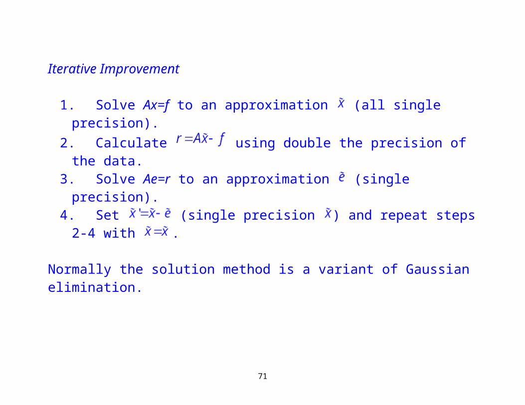
Iterative Improvement
1. Solve Ax=f to an approximation (all single precision).2. Calculate using double the precision of the data.3. Solve Ae=r to an approximation (single precision).4. Set (single precision ) and repeat steps 2-4 with .
Normally the solution method is a variant of Gaussian elimination.Note that . Since we cannot solve Ax=f exactly, we probably cannot solve Ae=r exactly, either.
Fact: If 1st has q digits correct. Then the 2nd will have 2q digits correct (assuming that 2q is less than the number of digits representable on your computer) and the nth will have nq digits correct (under a similar assumption as before).
Parallelization is straightforward: Use a parallel Gaussian elimination code and parallelize the residual calculation based on where the data resides.
52
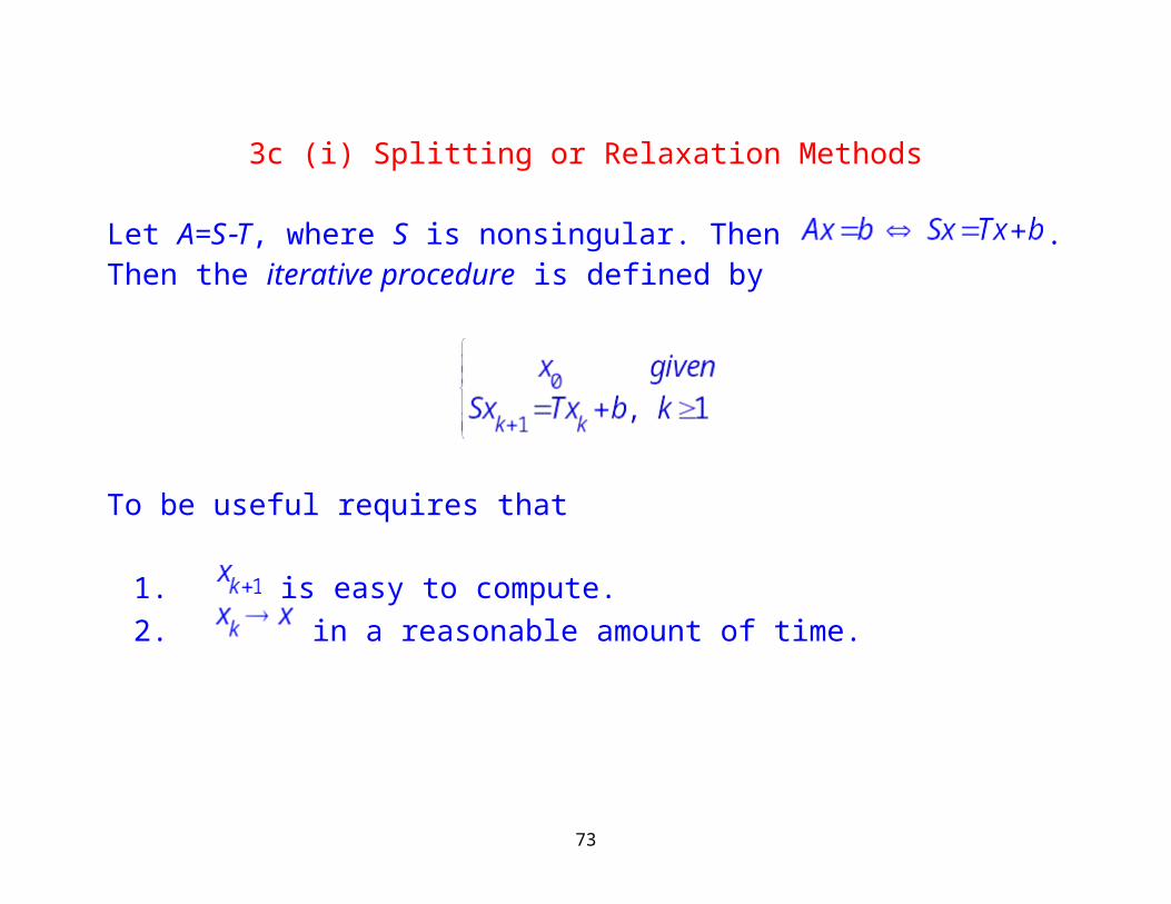
3c. Iterative Methods
3c (i) Splitting or Relaxation Methods
Let A=ST, where S is nonsingular. Then . Then the iterative procedure is defined by
To be useful requires that
1. is easy to compute.2. in a reasonable amount of time.
53
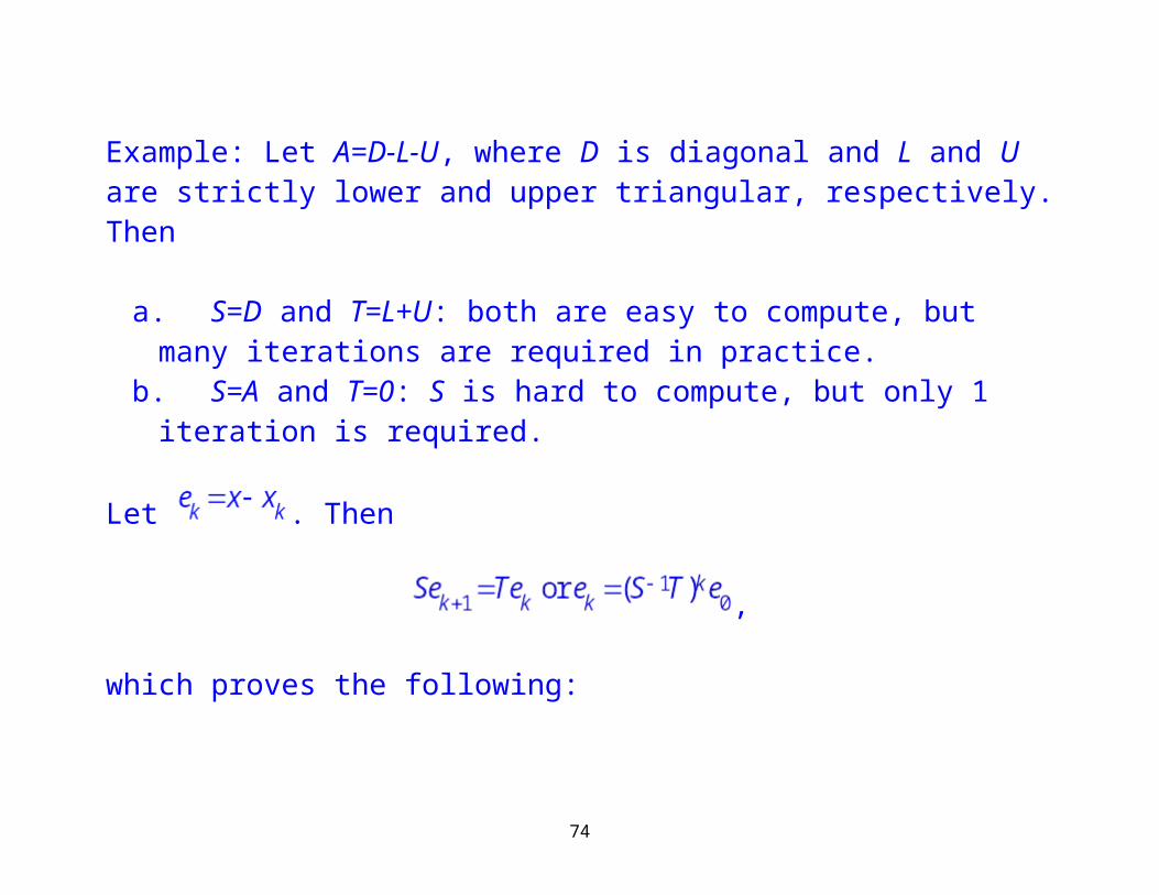
Example: Let A=D-L-U, where D is diagonal and L and U are strictly lower and upper triangular, respectively. Then
a. S=D and T=L+U: both are easy to compute, but many iterations are required in practice.
b. S=A and T=0: S is hard to compute, but only 1 iteration is required.
Let . Then
,
which proves the following:
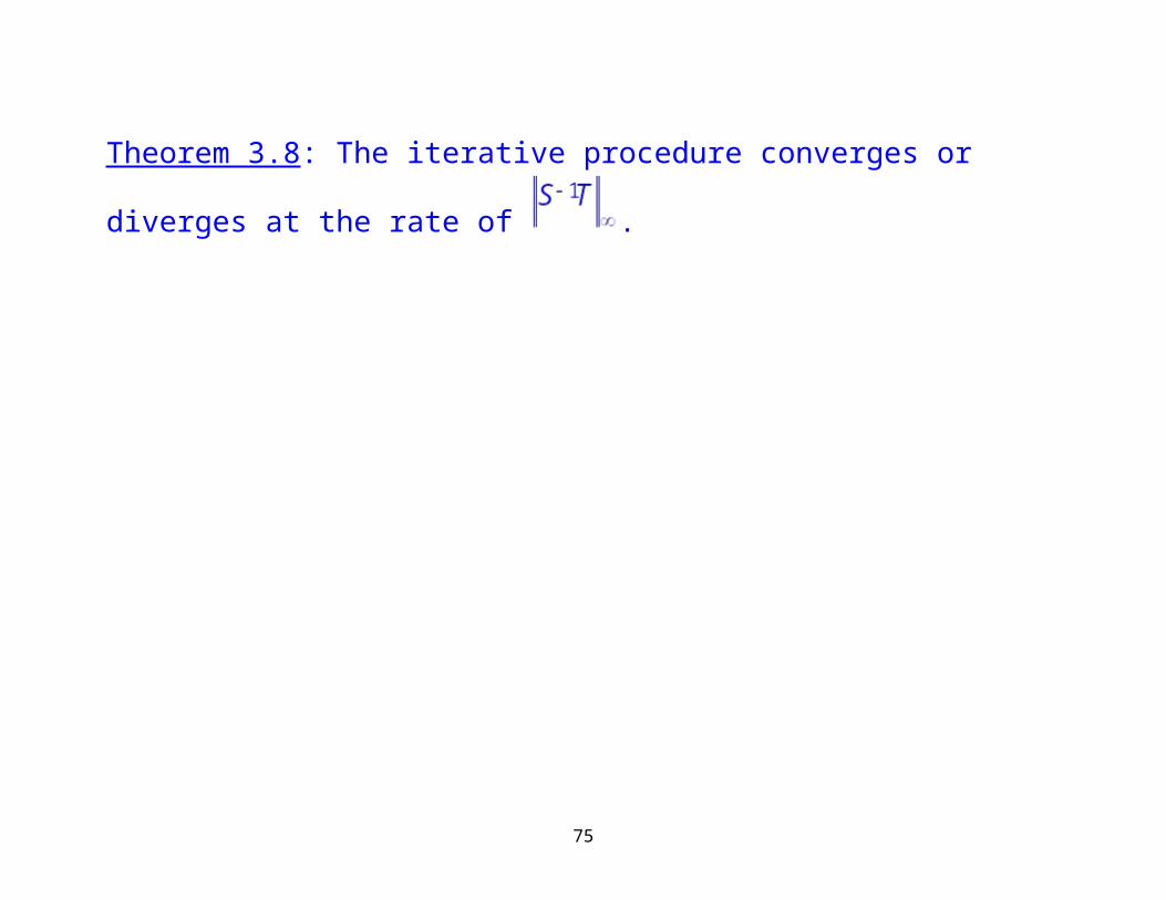
Theorem 3.8: The iterative procedure converges or diverges at the rate of
.
54
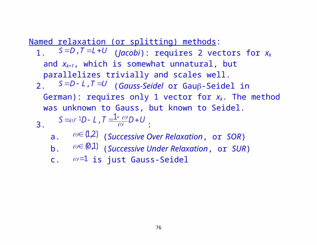
Named relaxation (or splitting) methods:1. (Jacobi): requires 2 vectors for xk and xk+1, which is
somewhat unnatural, but parallelizes trivially and scales well.2. (Gauss-Seidel or Gau-Seidel in German): requires only 1
vector for xk. The method was unknown to Gauss, but known to Seidel.
3. :a. (Successive Over Relaxation, or SOR)b. (Successive Under Relaxation, or SUR)c. is just Gauss-Seidel
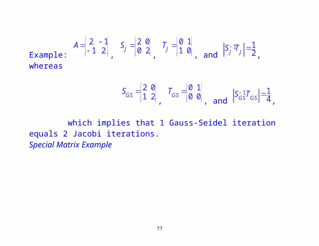
Example: , , , and , whereas
, , and ,
55
which implies that 1 Gauss-Seidel iteration equals 2 Jacobi iterations.Special Matrix Example
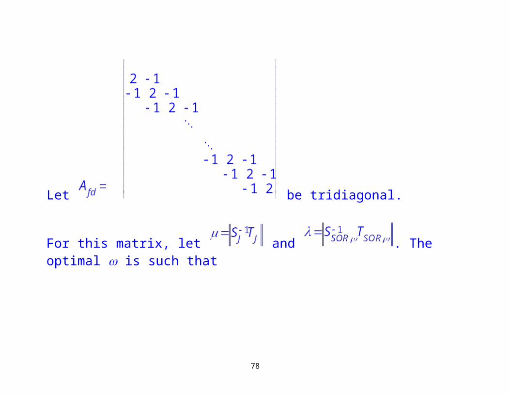
Let be tridiagonal.
For this matrix, let and . The optimal is such that
56
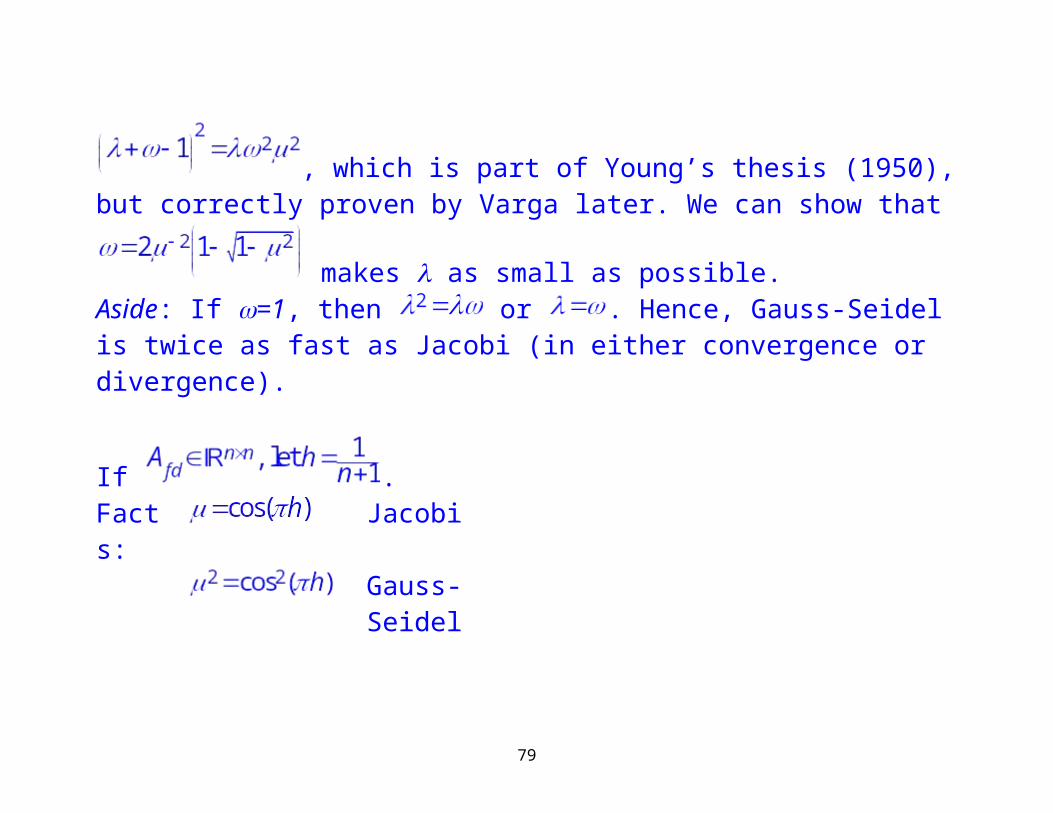
, which is part of Young’s thesis (1950), but correctly proven
by Varga later. We can show that makes as small as possible.Aside: If =1, then or . Hence, Gauss-Seidel is twice as fast as Jacobi (in either convergence or divergence).
If .Facts: Jacobi
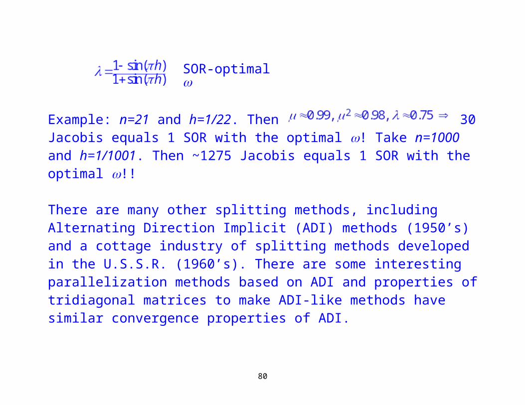
Gauss-SeidelSOR-optimal
Example: n=21 and h=1/22. Then 30 Jacobis equals 1 SOR with the optimal ! Take n=1000 and h=1/1001. Then ~1275 Jacobis equals 1 SOR with the optimal !!
57
There are many other splitting methods, including Alternating Direction Implicit (ADI) methods (1950’s) and a cottage industry of splitting methods developed in the U.S.S.R. (1960’s). There are some interesting parallelization methods based on ADI and properties of tridiagonal matrices to make ADI-like methods have similar convergence properties of ADI.
Parallelization of the Iterative Procedure
For Jacobi, parallelization is utterly trivial:1. Split up the unknowns onto processors.2. Each processor updates all of its unknowns.3. Each processor sends its unknowns to processors that need the updated
information.4. Continue iterating until done.
58
Common fallacies: When an element of the solution vector xk has a small enough element-
wise residual, stop updating the element. This leads to utterly wrong solutions since the residuals are affected by updates of neighbors after the element stops being updated.
Keep computing and use the last known update from neighboring processors. This leads to chattering and no element-wise convergence.
Asynchronous algorithms exist, but eliminate the chattering through extra calculations.
Parallel Gauss-Seidel and SOR are much, much harder. In fact, by and large, they do not exist. Googling efforts leads to an interesting set of papers that approximately parallelize Gauss-Seidel for a set of matrices with a very well known structures only. Even then, the algorithms are extremely complex.
59
Parallel Block-Jacobi is commonly used instead as an approximation. The matrix A is divided up into a number of blocks. Each block is assigned to a processor. Inside of each block, Jacobi is performed some number of iterations. Data is exchanged between processors and the iteration continues.
See the book (absolutely shameless plug),
C. C. Douglas, G. Haase, and U. Langer, A Tutorial on Elliptic PDE Solvers and Their Parallelization, SIAM Books, Philadelphia, 2003
for how to do parallelization of iterative methods for matrices that commonly occur when solving partial differential equations (what else would you ever want to solve anyway???).
60
3c (ii) Krylov Space Methods
Conjugate Gradients
Let A be symmetric, positive definite, i.e.,
A=AT and .
The conjugate gradient iteration method for the solution of Ax+b=0 is defined as follows with r=r(x)=Ax+b:
x0 arbitrary (approximate solution)r0=Ax0+b (approximate residual)w0=r0 (search direction)
61
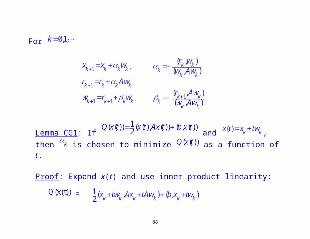
For
Lemma CG1: If and , then is chosen to minimize as a function of t.
Proof: Expand x(t) and use inner product linearity:
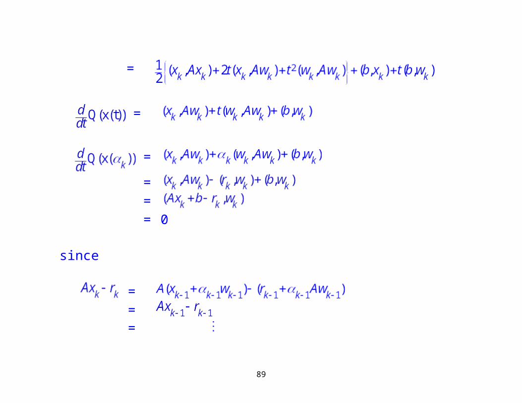
=
=
62
=
=
=== 0
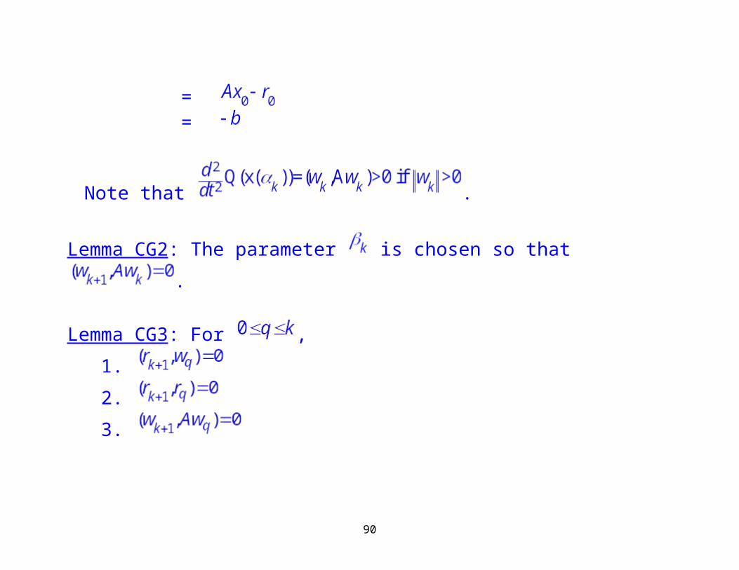
since
=== ==
63
Note that .
Lemma CG2: The parameter is chosen so that .
Lemma CG3: For ,
1.
2.
3.
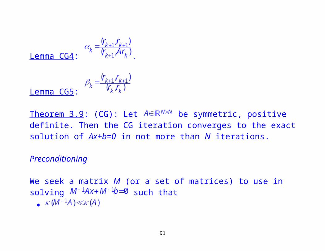
Lemma CG4: .
64
Lemma CG5:
Theorem 3.9: (CG): Let be symmetric, positive definite. Then the CG iteration converges to the exact solution of Ax+b=0 in not more than N iterations.
Preconditioning
We seek a matrix M (or a set of matrices) to use in solving such that
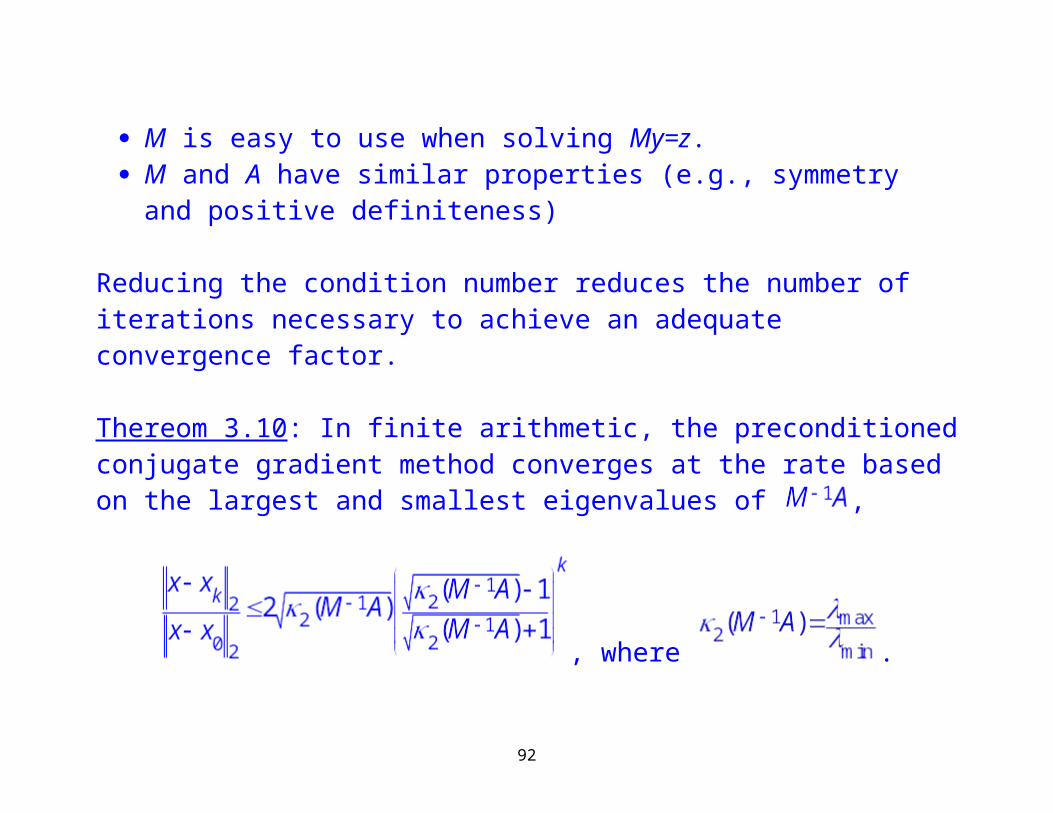
M is easy to use when solving My=z. M and A have similar properties (e.g., symmetry and positive definiteness)
Reducing the condition number reduces the number of iterations necessary to achieve an adequate convergence factor.
65
Thereom 3.10: In finite arithmetic, the preconditioned conjugate gradient method converges at the rate based on the largest and smallest eigenvalues of
,
, where .
Proof: See Golub and Van Loan or many other numerical linear algebra books.
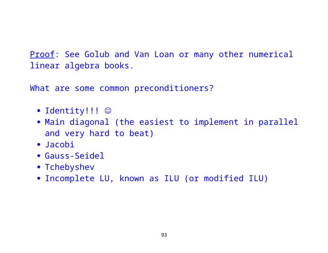
What are some common preconditioners?
Identity!!! Main diagonal (the easiest to implement in parallel and very hard to beat) Jacobi Gauss-Seidel
66
Tchebyshev Incomplete LU, known as ILU (or modified ILU)
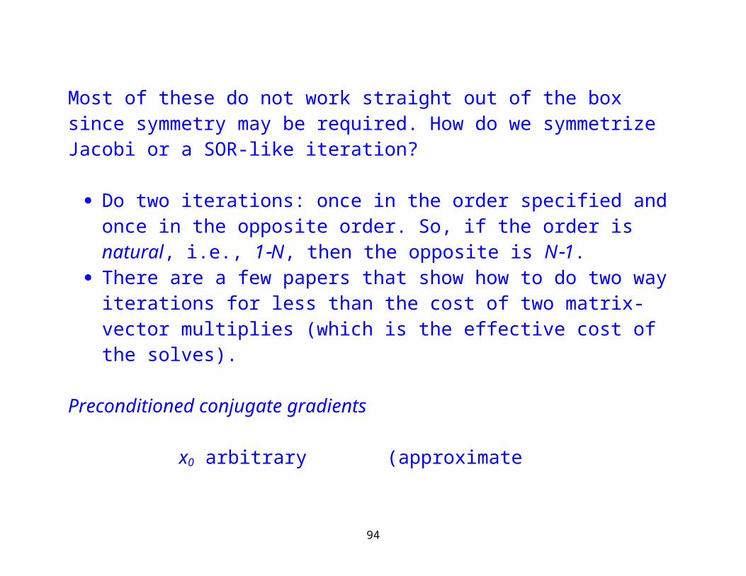
Most of these do not work straight out of the box since symmetry may be required. How do we symmetrize Jacobi or a SOR-like iteration?
Do two iterations: once in the order specified and once in the opposite order. So, if the order is natural, i.e., 1N, then the opposite is N1.
There are a few papers that show how to do two way iterations for less than the cost of two matrix-vector multiplies (which is the effective cost of the solves).
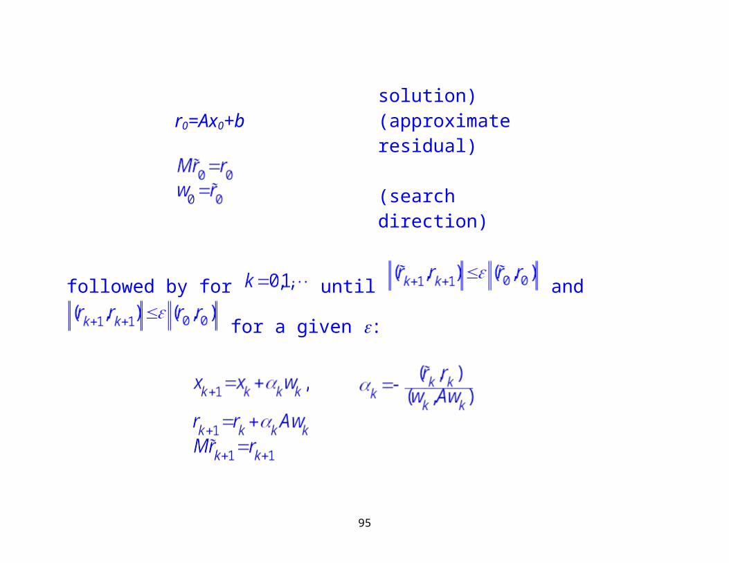
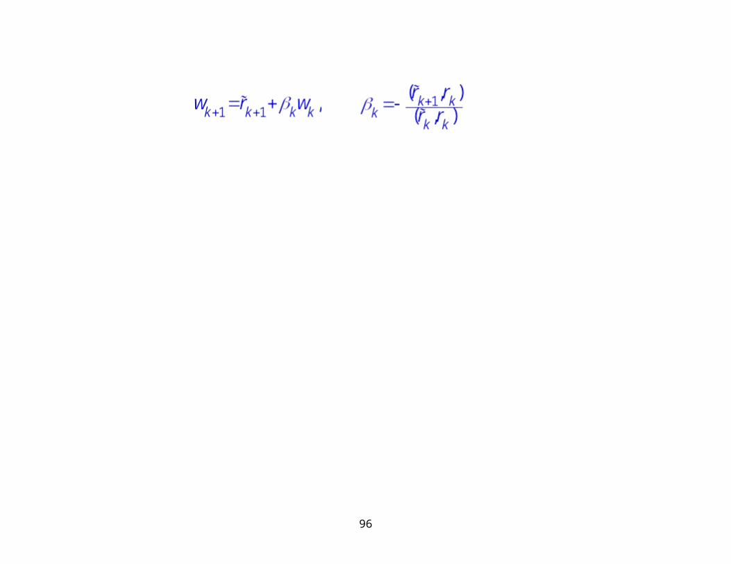
Preconditioned conjugate gradients
x0 arbitrary (approximate solution)r0=Ax0+b (approximate residual)
(search direction)
67
followed by for until and for a given :
68
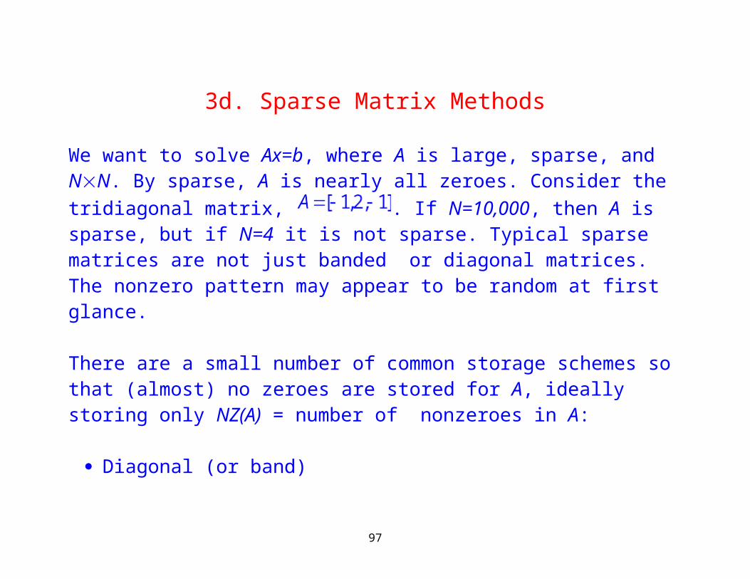
3d. Sparse Matrix Methods
We want to solve Ax=b, where A is large, sparse, and NN. By sparse, A is nearly all zeroes. Consider the tridiagonal matrix, . If N=10,000, then A is sparse, but if N=4 it is not sparse. Typical sparse matrices are not just banded or diagonal matrices. The nonzero pattern may appear to be random at first glance.
There are a small number of common storage schemes so that (almost) no zeroes are stored for A, ideally storing only NZ(A) = number of nonzeroes in A:
Diagonal (or band) Profile Row or column (and several variants) Any of the above for blocks
The schemes all work in parallel, too, for the local parts of A. Sparse matrices arise in a very large percentage of problems on large parallel computers.
69
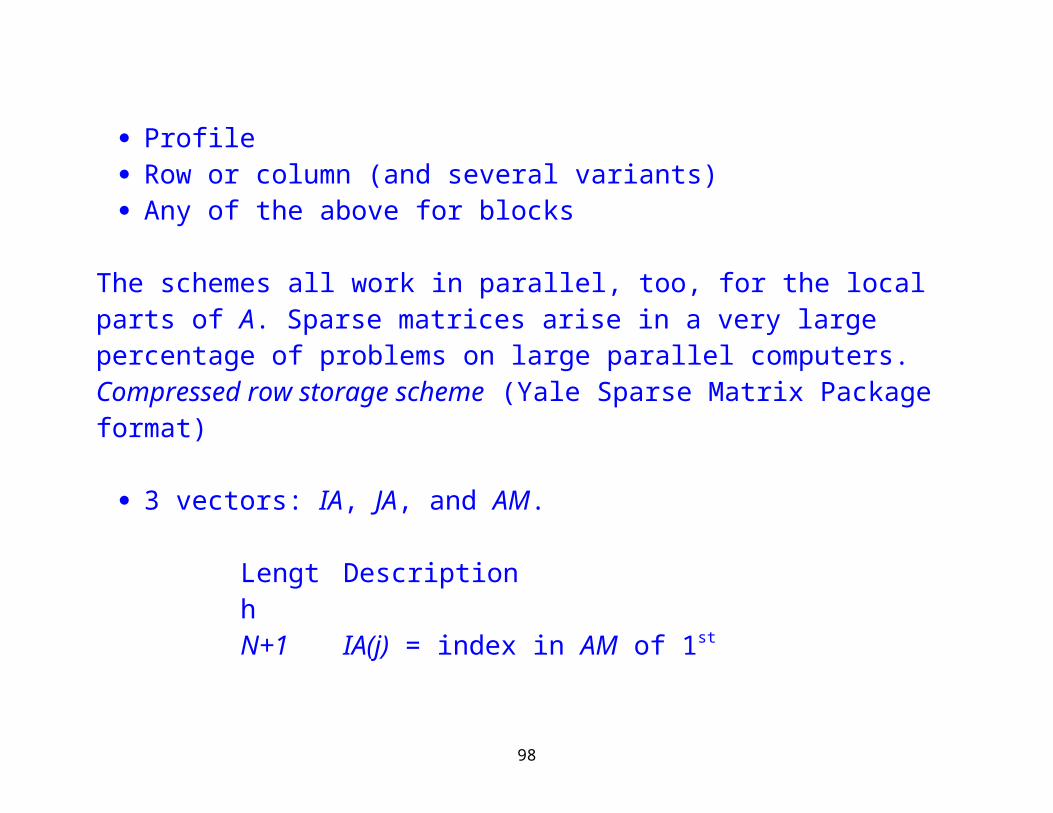
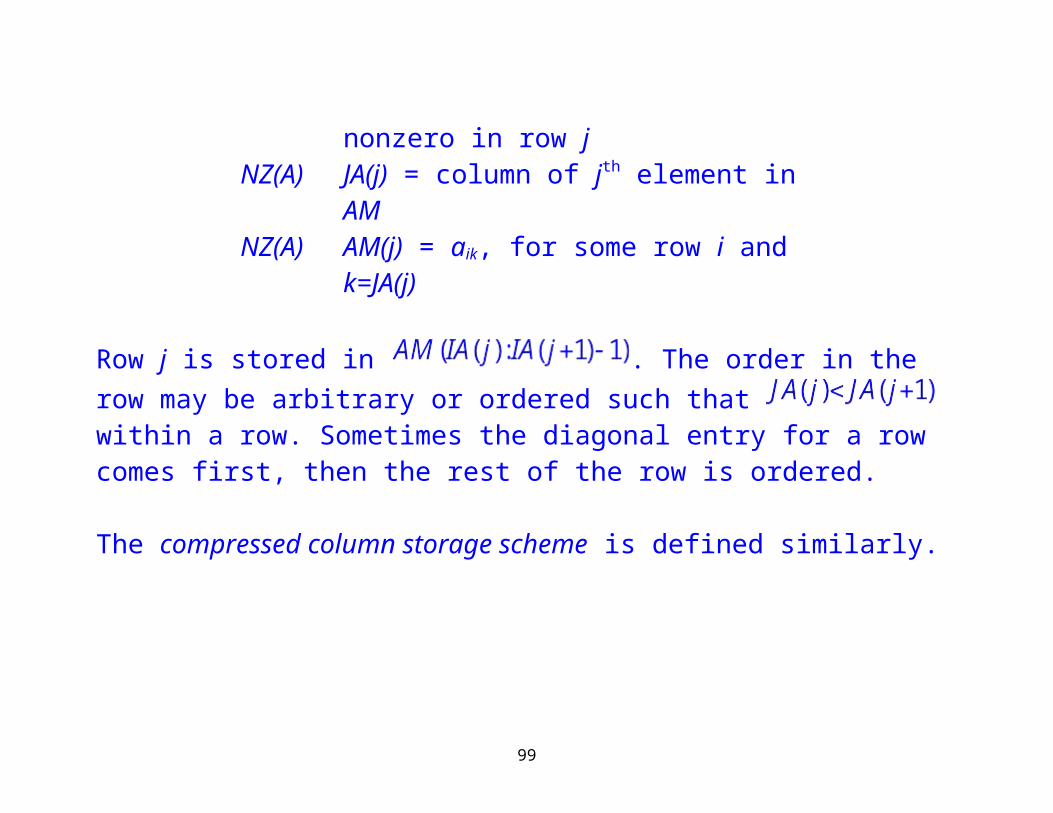
Compressed row storage scheme (Yale Sparse Matrix Package format)
3 vectors: IA, JA, and AM.
Length DescriptionN+1 IA(j) = index in AM of 1st nonzero in row jNZ(A) JA(j) = column of jth element in AMNZ(A) AM(j) = aik, for some row i and k=JA(j)
Row j is stored in . The order in the row may be arbitrary or ordered such that within a row. Sometimes the diagonal entry for a row comes first, then the rest of the row is ordered.
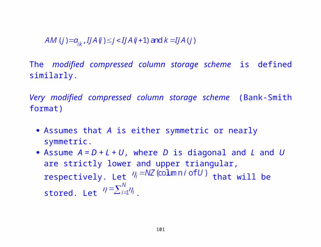
The compressed column storage scheme is defined similarly.
70
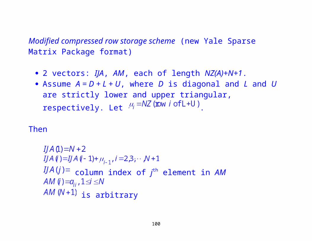
Modified compressed row storage scheme (new Yale Sparse Matrix Package format)
2 vectors: IJA, AM, each of length NZ(A)+N+1. Assume A = D + L + U, where D is diagonal and L and U are strictly lower
and upper triangular, respectively. Let .
Then
column index of jth element in AM
is arbitrary
The modified compressed column storage scheme is defined similarly.
71
Very modified compressed column storage scheme (Bank-Smith format)
Assumes that A is either symmetric or nearly symmetric. Assume A = D + L + U, where D is diagonal and L and U are strictly lower
and upper triangular, respectively. Let that will be
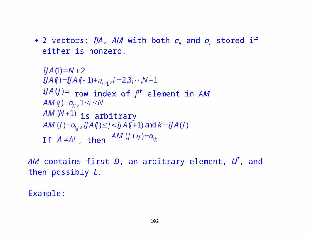
stored. Let . 2 vectors: IJA, AM with both aij and aji stored if either is nonzero.
row index of jth element in AM
is arbitrary
If , then
72
AM contains first D, an arbitrary element, UT, and then possibly L.
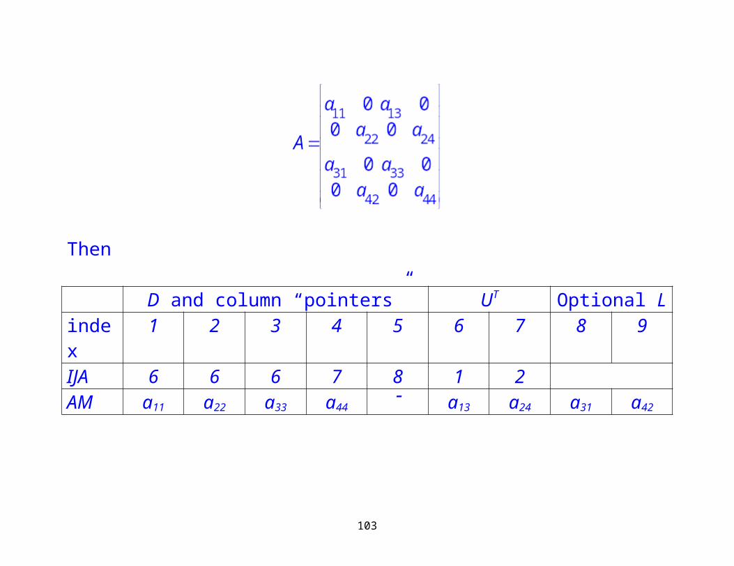
Example:
Then
D and column “pointers” UT Optional Lindex 1 2 3 4 5 6 7 8 9IJA 6 6 6 7 8 1 2AM a11 a22 a33 a44 a13 a24 a31 a42
73
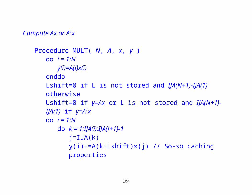
Compute Ax or ATx
Procedure MULT( N, A, x, y )do i = 1:N
y(i)=A(i)x(i)enddoLshift=0 if L is not stored and IJA(N+1)-IJA(1) otherwiseUshift=0 if y=Ax or L is not stored and IJA(N+1)-IJA(1) if y=ATxdo i = 1:N
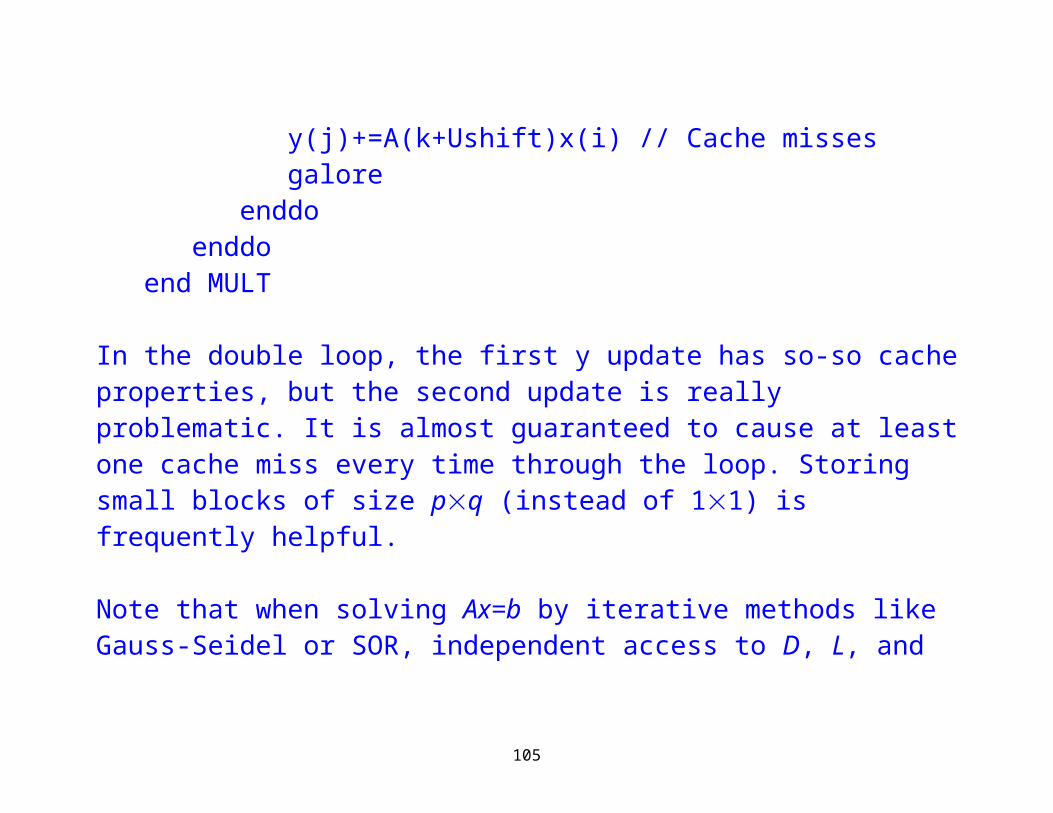
do k = 1:IJA(i):IJA(i+1)-1j=IJA(k)y(i)+=A(k+Lshift)x(j) // So-so caching propertiesy(j)+=A(k+Ushift)x(i) // Cache misses galore
enddoenddo
end MULT
74
In the double loop, the first y update has so-so cache properties, but the second update is really problematic. It is almost guaranteed to cause at least one cache miss every time through the loop. Storing small blocks of size pq (instead of 11) is frequently helpful.
Note that when solving Ax=b by iterative methods like Gauss-Seidel or SOR, independent access to D, L, and U is required. These algorithms can be implemented fairly easily on a single processor core.
Sparse Gaussian elimination
We want to factor A=LDU. Without loss of generality, we assume that A is already reordered so that this is accomplished without pivoting. The solution is computed using forward, diagonal, and backward substitutions:
There are 3 phases:
75
1. symbolic factorization (determine the nonzero structure of U and possibly L,
2. numeric factorization (compute LDU), and3. forward/backward substitution (compute x).
Let denote the ordered, undirected graph corresponding to the matrix
A. is the virtex set, is the edge set, and
virtex adjaceny set is .
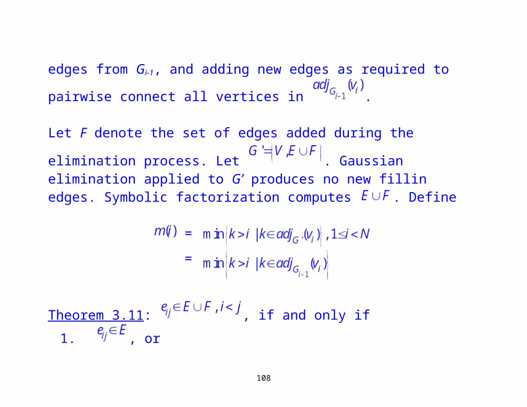
Gaussian elimination corresponds to a sequence of elimination graphs Gi, 0i<N. Let G0=G. Define Gi from Gi-1, i>0, by removing vi from Gi-1 and all of its incident edges from Gi-1, and adding new edges as required to pairwise
connect all vertices in .
76
Let F denote the set of edges added during the elimination process. Let
. Gaussian elimination applied to G’ produces no new fillin edges. Symbolic factorization computes . Define
=
=
Theorem 3.11: , if and only if
1. , or
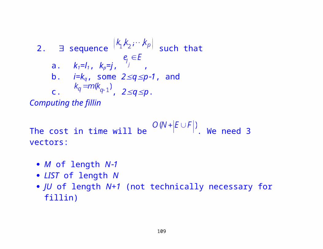
2. sequence such that
a. k1=l1, kp=j, ,b. i=kq, some 2qp1, and
c. , 2qp.
77
Computing the fillin
The cost in time will be . We need 3 vectors:
M of length N1 LIST of length N JU of length N+1 (not technically necessary for fillin)
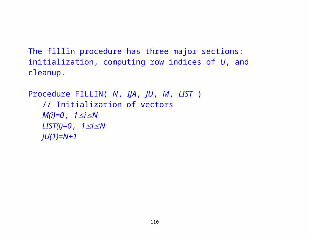
The fillin procedure has three major sections: initialization, computing row indices of U, and cleanup.
Procedure FILLIN( N, IJA, JU, M, LIST )// Initialization of vectorsM(i)=0, 1iNLIST(i)=0, 1iNJU(1)=N+1
78
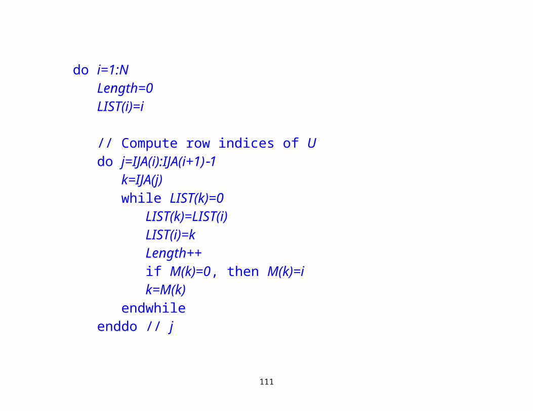
do i=1:NLength=0LIST(i)=i
// Compute row indices of Udo j=IJA(i):IJA(i+1)1
k=IJA(j)while LIST(k)=0
LIST(k)=LIST(i)LIST(i)=kLength++if M(k)=0, then M(k)=ik=M(k)
endwhileenddo // jJU(i+1)=JU(i)+Length
79
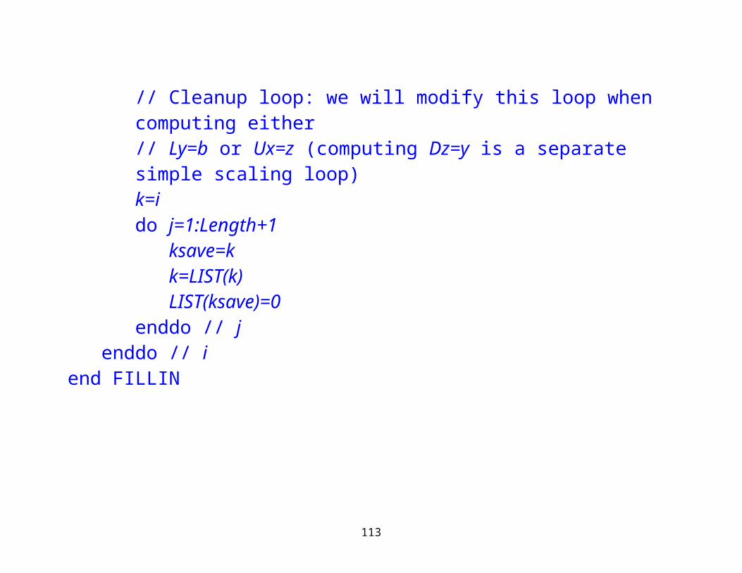
// Cleanup loop: we will modify this loop when computing either// Ly=b or Ux=z (computing Dz=y is a separate simple scaling loop)k=ido j=1:Length+1
ksave=kk=LIST(k)LIST(ksave)=0
enddo // jenddo // i
end FILLIN
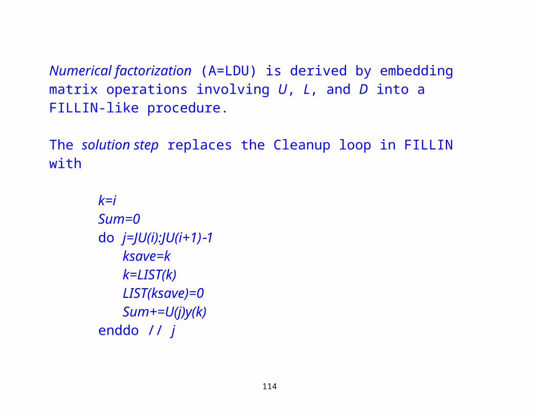
Numerical factorization (A=LDU) is derived by embedding matrix operations involving U, L, and D into a FILLIN-like procedure.
The solution step replaces the Cleanup loop in FILLIN with
k=iSum=0
80
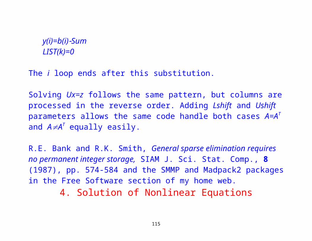
do j=JU(i):JU(i+1)1ksave=kk=LIST(k)LIST(ksave)=0Sum+=U(j)y(k)
enddo // jy(i)=b(i)SumLIST(k)=0
The i loop ends after this substitution.
Solving Ux=z follows the same pattern, but columns are processed in the reverse order. Adding Lshift and Ushift parameters allows the same code handle both cases A=AT and AAT equally easily.
R.E. Bank and R.K. Smith, General sparse elimination requires no permanent integer storage, SIAM J. Sci. Stat. Comp., 8 (1987), pp. 574-584 and the SMMP and Madpack2 packages in the Free Software section of my home web.
81
4. Solution of Nonlinear Equations
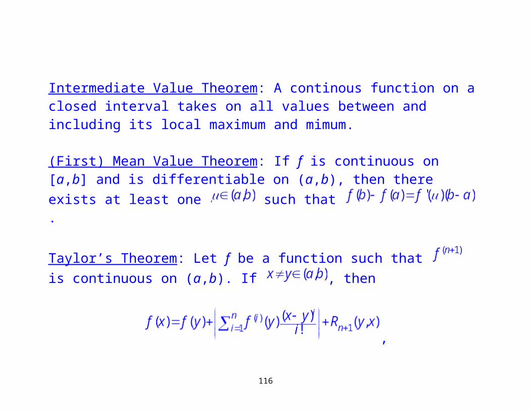
Intermediate Value Theorem: A continous function on a closed interval takes on all values between and including its local maximum and mimum.
(First) Mean Value Theorem: If f is continuous on [a,b] and is differentiable on (a,b), then there exists at least one such that .
Taylor’s Theorem: Let f be a function such that is continuous on (a,b). If , then
,where between x and y such that
82
.Given y=f(x), find all s such that f(s)=0.
Backtracking Schemes
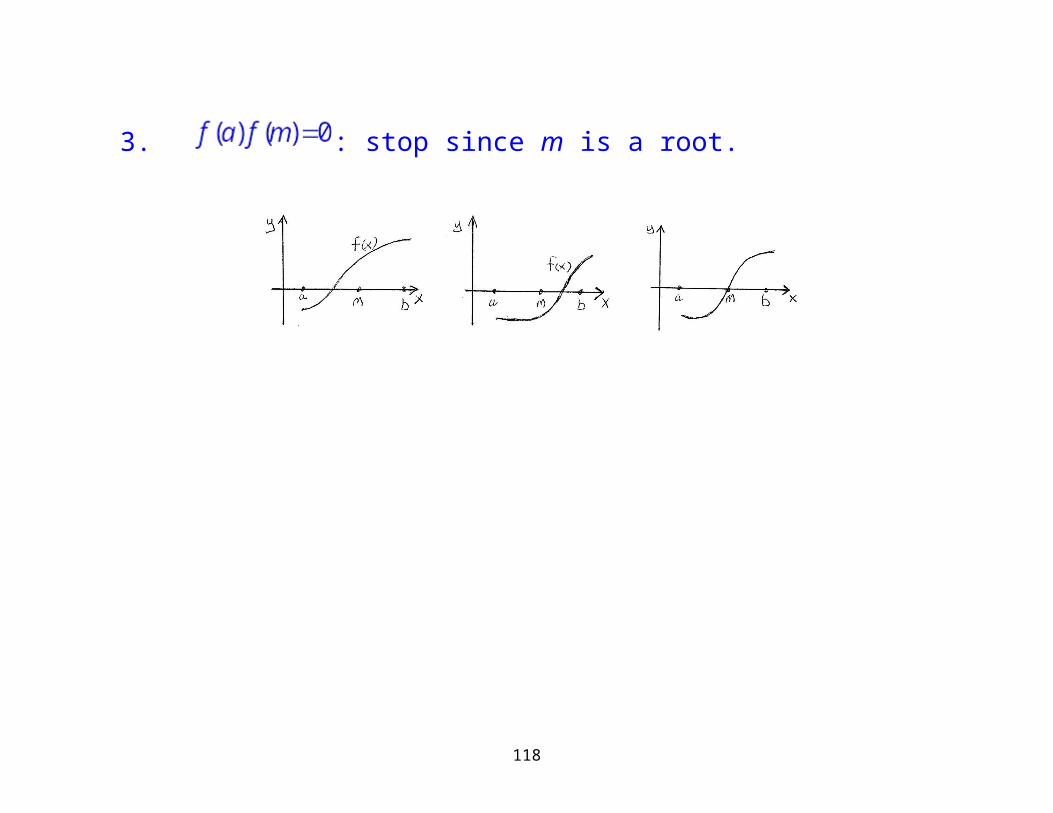
Suppose and f is continuous on [a,b].
Bisection method: Let . Then either1. : replace b by m. 2. : replace a by m. 3. : stop since m is a root.
83
84
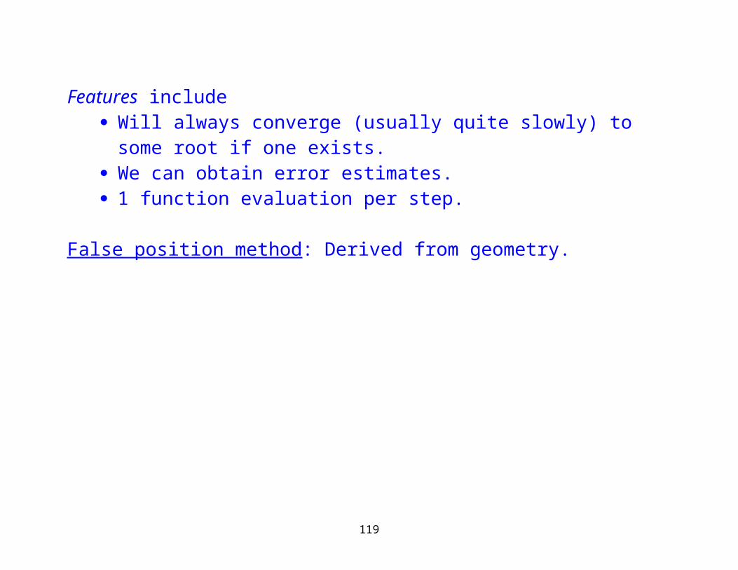
Features include Will always converge (usually quite slowly) to some root if one exists. We can obtain error estimates. 1 function evaluation per step.
False position method: Derived from geometry.
85
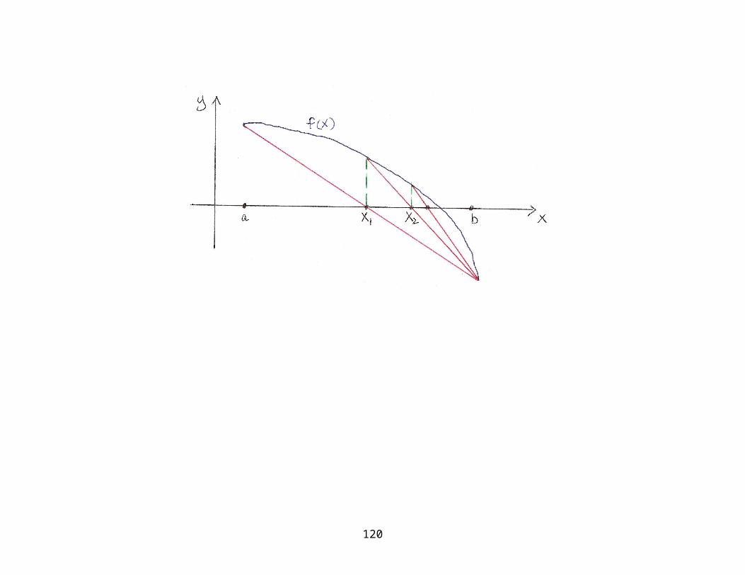
First we determine the secant line from to :
.
The secant line crosses the x-axis when , where
or .
Then a root lies in either or depending on sign of as before. We replace a or b with depending on which interval the root lies and repeat until we get (close enough) to the root.
86
Features include
Usually converges faster than the Bisection method, but is quite slow.. Very old method: first reference is in the Indian mathematics text Vaishali
Ganit (circa 3rd century BC). It was known in China by the 2nd century AD and by Fibonacci in 1202. Middle Eastern mathematicians kept the method alive during the European Dark Ages.
The method can get stuck, however. In this case, it can be unstuck (and speeded up) by choosing either
or .
Modifications like this are called the Illinois method and date to the 1970’s.
87
Fixed point methods: Construct a function g(s) such that .
Example: .
Constructing a good fixed point method is easy. The motivation is to look at a function y=g(x) and see when g(x) intersects y=x.
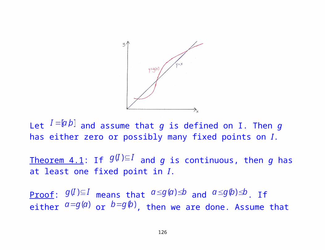
Let and assume that g is defined on I. Then g has either zero or possibly many fixed points on I.
88
Theorem 4.1: If and g is continuous, then g has at least one fixed point in I.
Proof: means that and . If either or , then we are done. Assume that is not the case: hence, and
. For , F is continuous and and . Thus, by the initial value theorem, there exists at least one such that
. QED
Why are Theorem 4.1’s requirements reasonable? : s cannot equal g(s) if not . Continuity: if g is discontinuous, the graph of g may lie partly above and
below y=x without an intersection.
Theorem 4.2: If and , then such that g(s)=s.
89
Proof: Suppose are both fixed points of g. The mean value theorem
with has the property that
,
which is a contradiction. QED
Note that the condition on must be continuous.
90
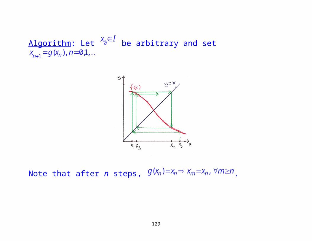
Algorithm: Let be arbitrary and set
Note that after n steps, .
91
Theorem 4.3: Let and . For , the sequence
converges to the fixed point s and the nth error satisfies
.
Note that Theorem 4.3 is a nonlocal convergence theorem because s is fixed, a known interval I is assumed, and convergence is for any .
Proof: (convergence) Recall that s is unique. For any n, between xn-1 and s such that
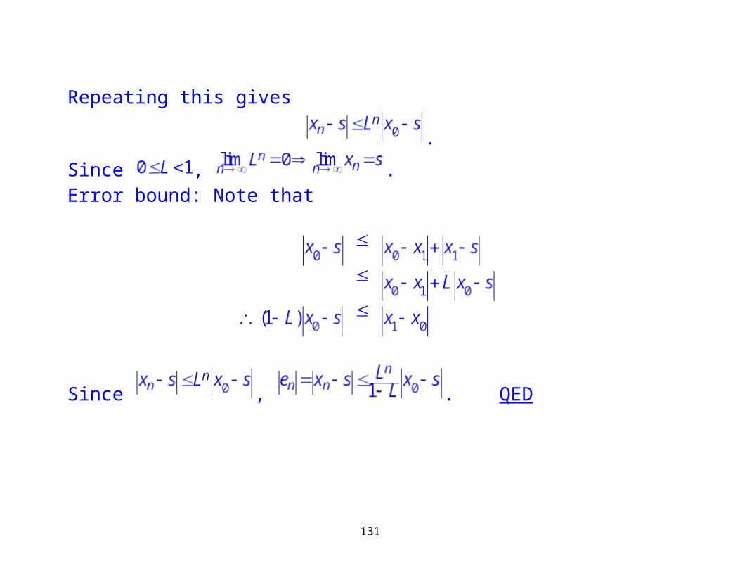
.Repeating this gives
.
92
Since , .Error bound: Note that
Since , . QED
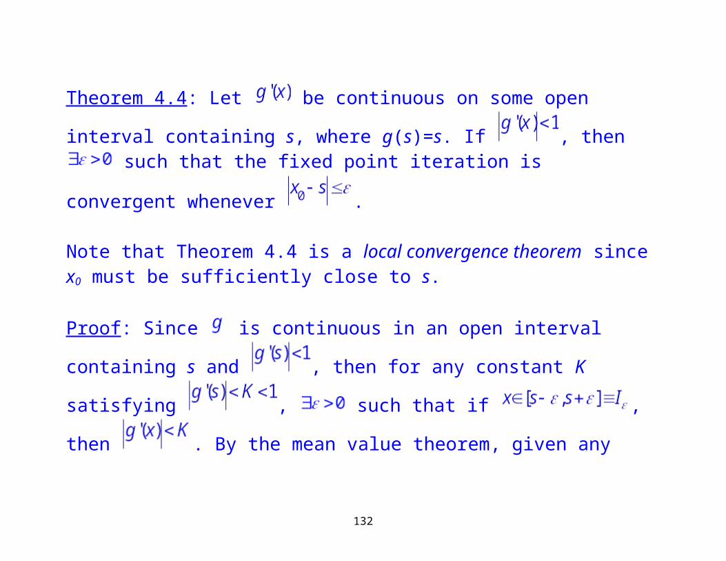
Theorem 4.4: Let be continuous on some open interval containing s, where
g(s)=s. If , then such that the fixed point iteration is convergent
whenever .
93
Note that Theorem 4.4 is a local convergence theorem since x0 must be sufficiently close to s.
Proof: Since is continuous in an open interval containing s and , then
for any constant K satisfying , such that if ,
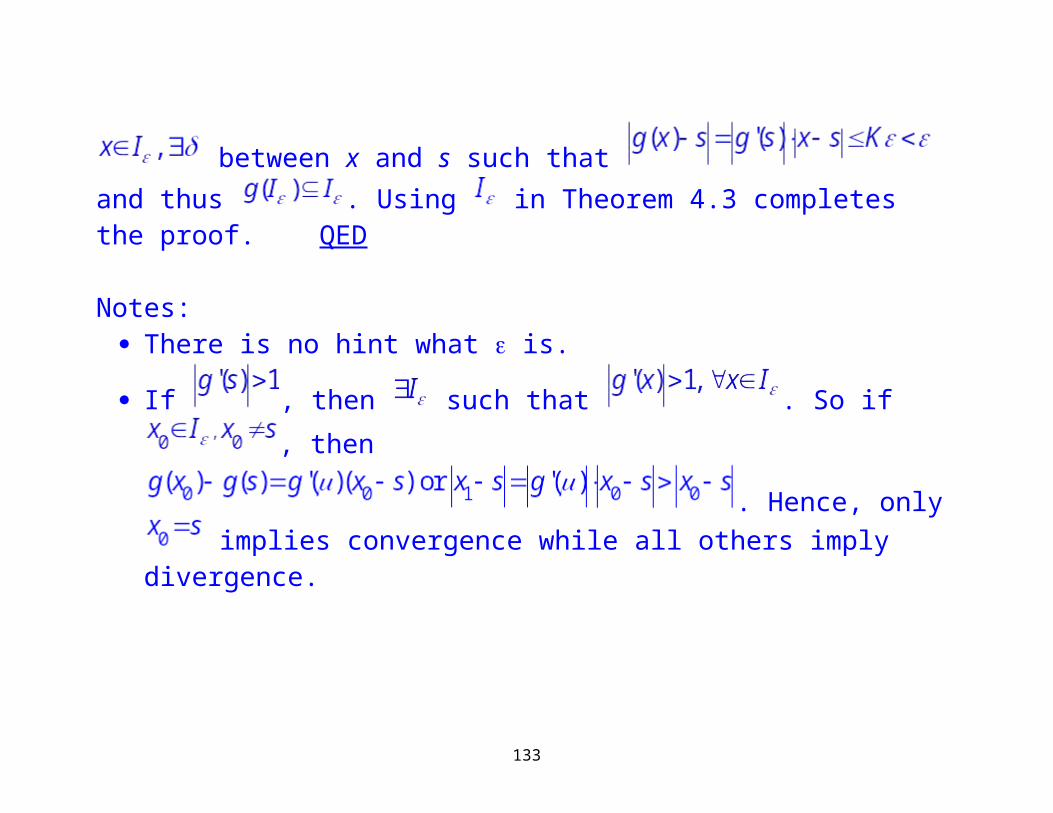
then . By the mean value theorem, given any between x and
s such that and thus . Using in Theorem 4.3 completes the proof. QED
Notes: There is no hint what is.
If , then such that . So if , then
. Hence, only implies convergence while all others imply divergence.
94
95
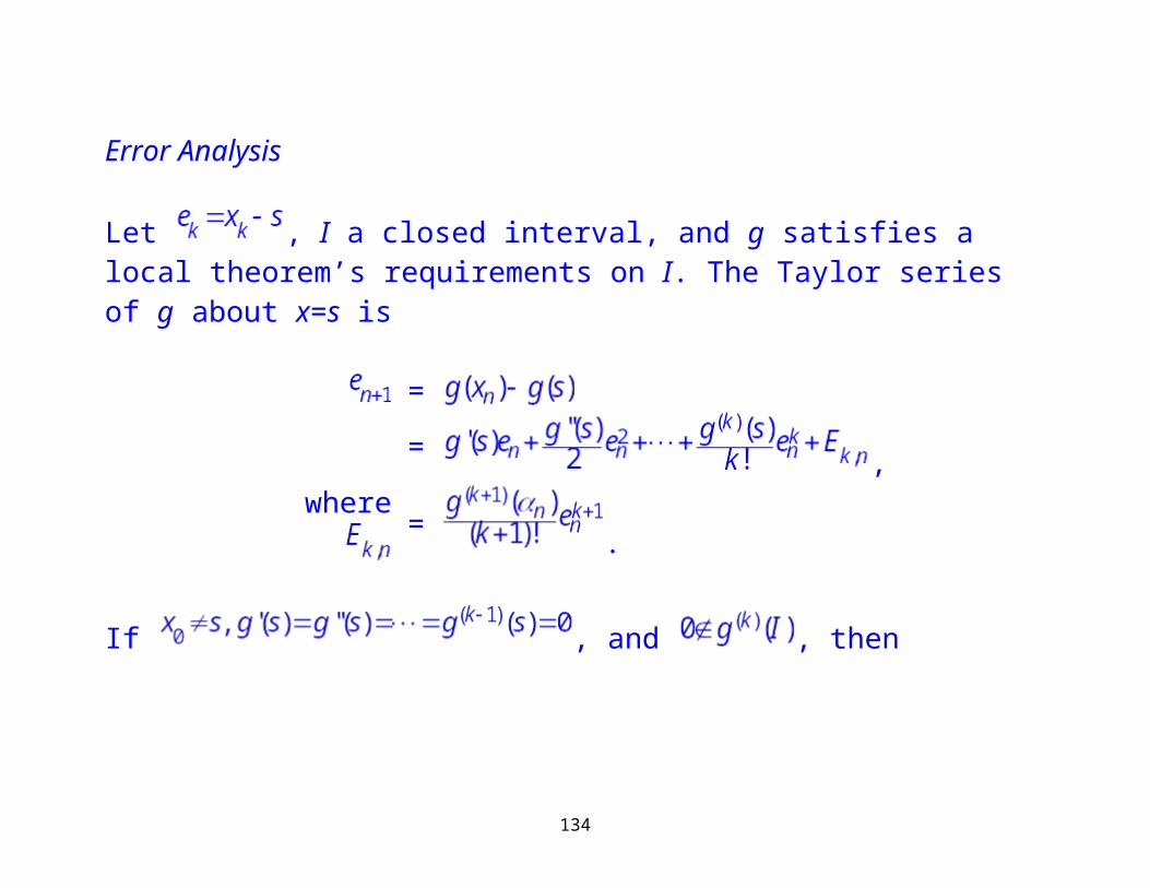
Error Analysis
Let , I a closed interval, and g satisfies a local theorem’s requirements on I. The Taylor series of g about x=s is
=
= ,
where =.
If , and , then
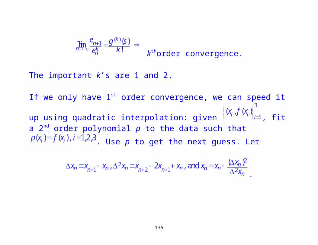
kthorder convergence.
The important k’s are 1 and 2.
96
If we only have 1st order convergence, we can speed it up using quadratic
interpolation: given , fit a 2nd order polynomial p to the data such that . Use p to get the next guess. Let
.
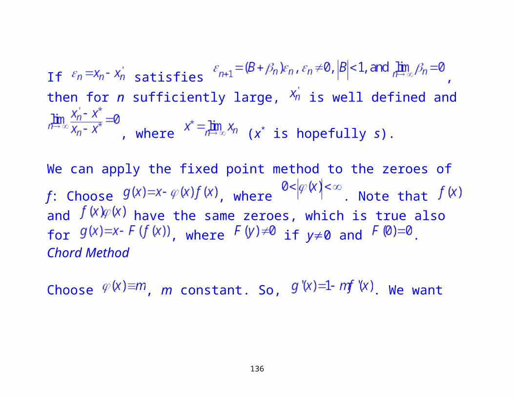
If satisfies , then for n
sufficiently large, is well defined and , where (x* is hopefully s).
We can apply the fixed point method to the zeroes of f: Choose
, where . Note that and have the
97
same zeroes, which is true also for , where if y0 and .
Chord Method
Choose , m constant. So, . We want
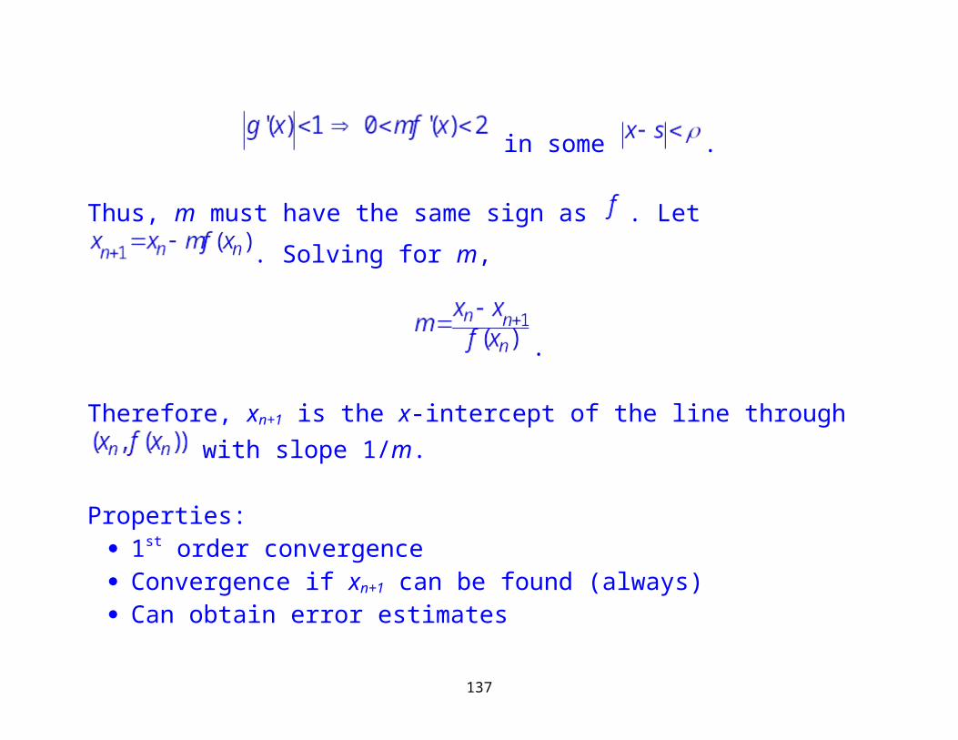
in some .
Thus, m must have the same sign as . Let . Solving for m,
.
Therefore, xn+1 is the x-intercept of the line through with slope 1/m.
Properties:
98
1st order convergence Convergence if xn+1 can be found (always) Can obtain error estimates
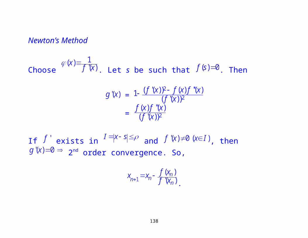
Newton’s Method
Choose . Let s be such that . Then
=
=
If exists in and , then 2nd order convergence. So,
.
99
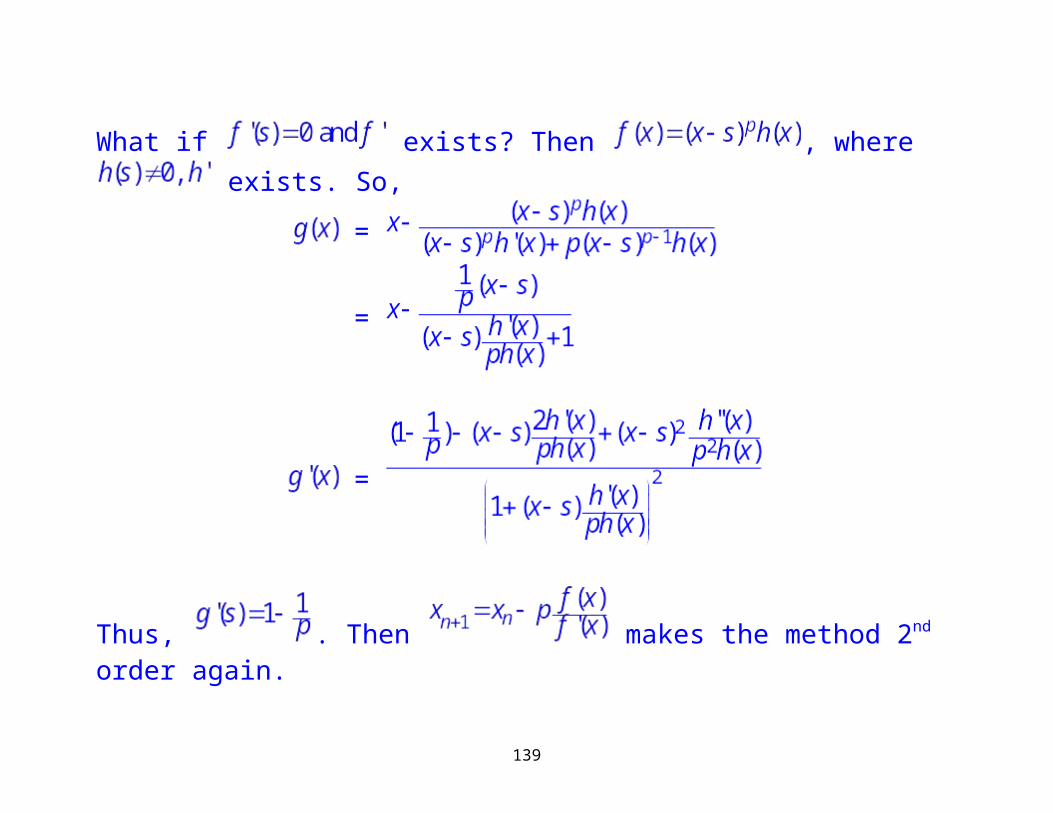
What if exists? Then , where exists. So,
=
=
=
Thus, . Then makes the method 2nd order again.
100
101
Properties: 2nd order convergence Evaluation of both and .
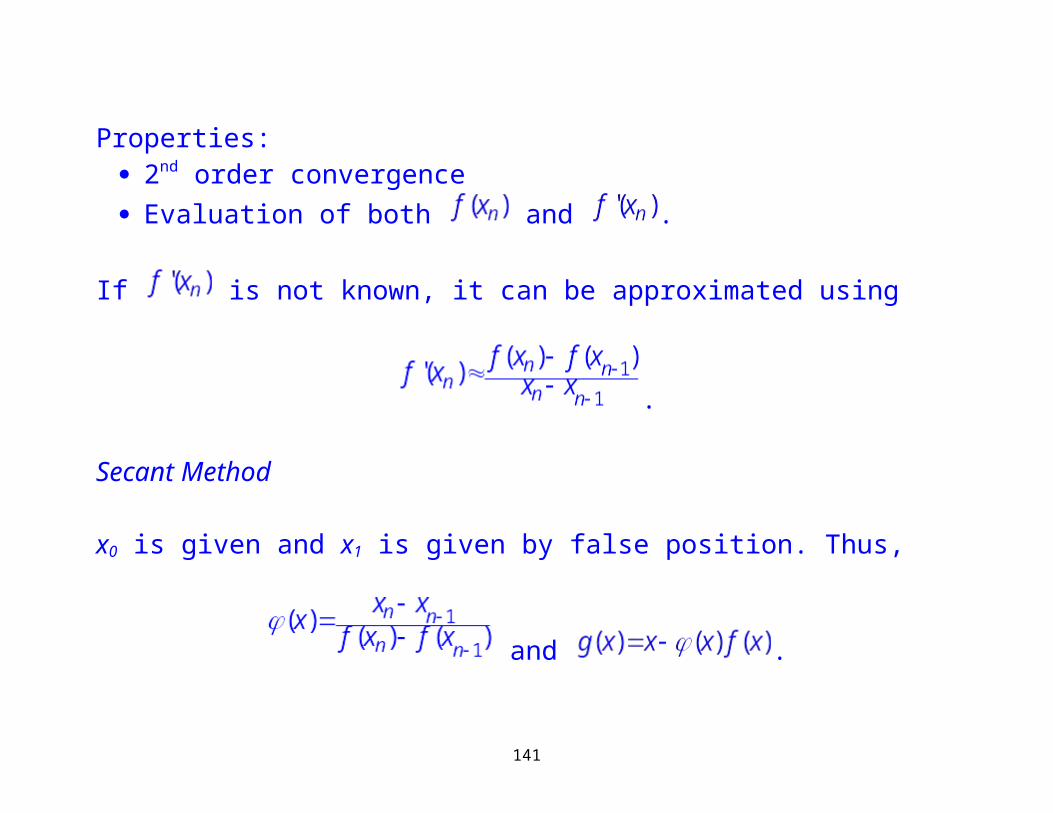
If is not known, it can be approximated using
.
Secant Method
x0 is given and x1 is given by false position. Thus,
and .
102
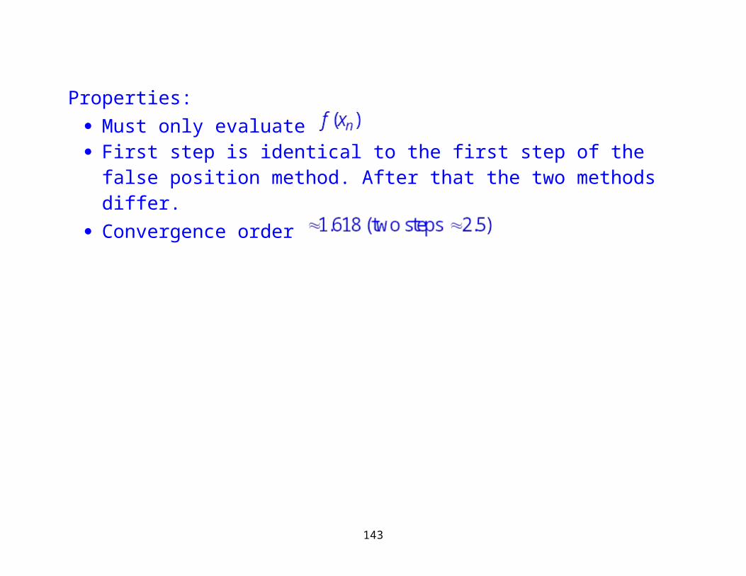
Properties: Must only evaluate First step is identical to the first step of the false position method. After that
the two methods differ. Convergence order
103
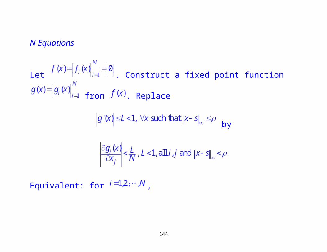
N Equations
Let . Construct a fixed point function from . Replace
by
Equivalent: for ,
.Thus,
104
Thus, .
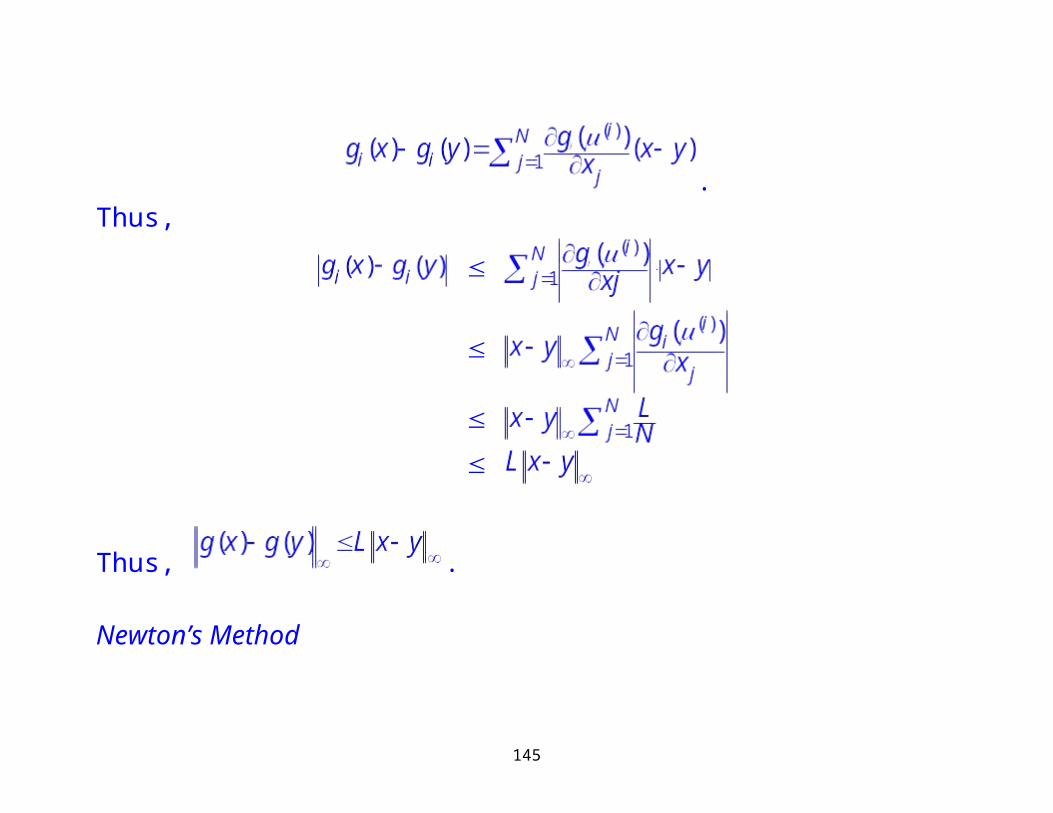
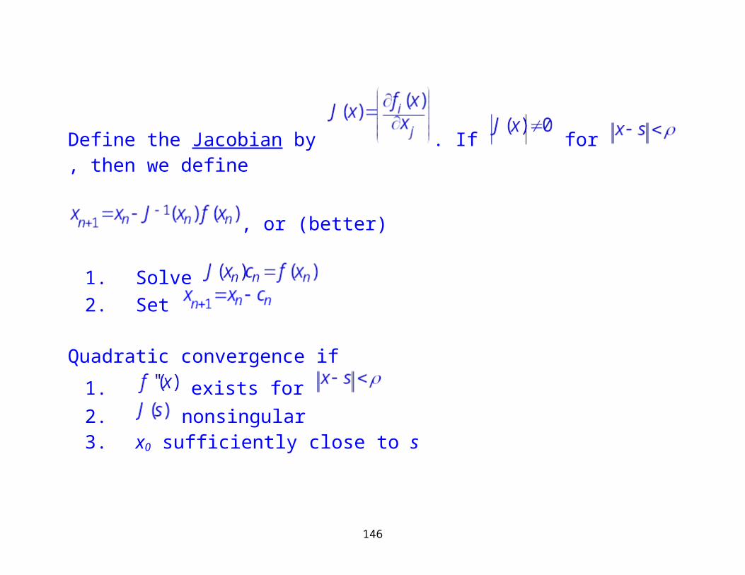
Newton’s Method
Define the Jacobian by . If for , then we define
105
, or (better)
1. Solve 2. Set
Quadratic convergence if
1. exists for 2. nonsingular3. x0 sufficiently close to s
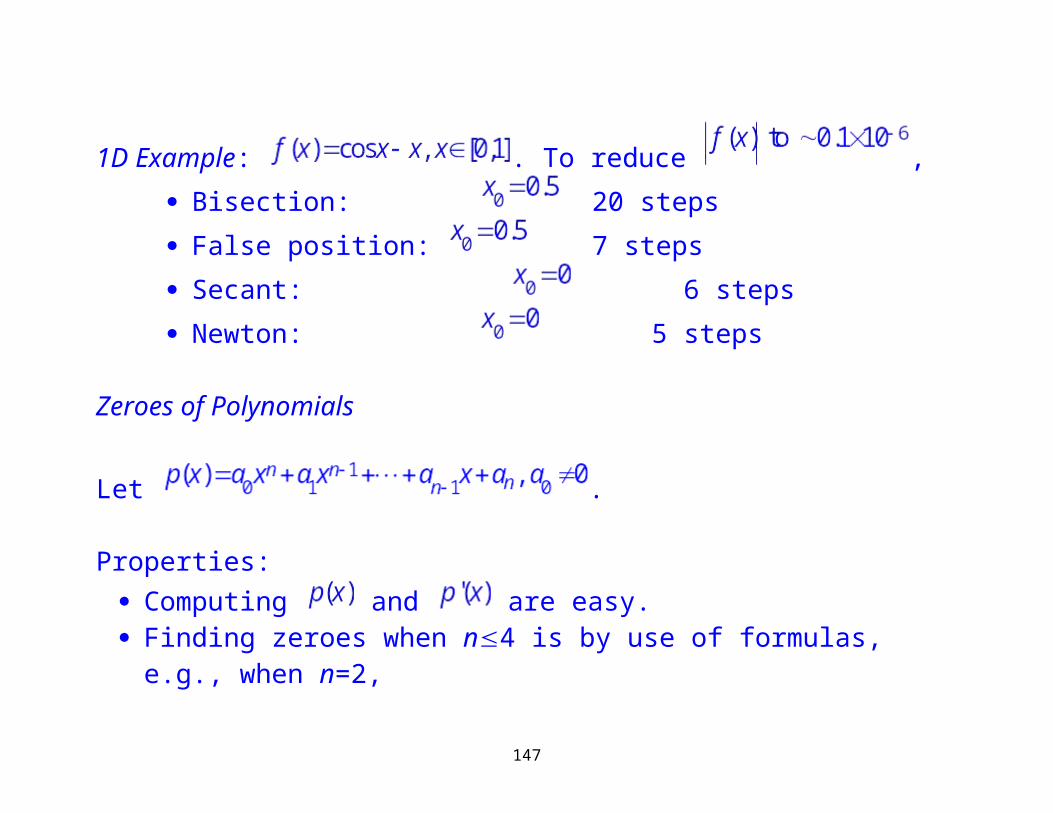
1D Example: . To reduce , Bisection: 20 steps False position: 7 steps Secant: 6 steps
106
Newton: 5 steps
Zeroes of Polynomials
Let .
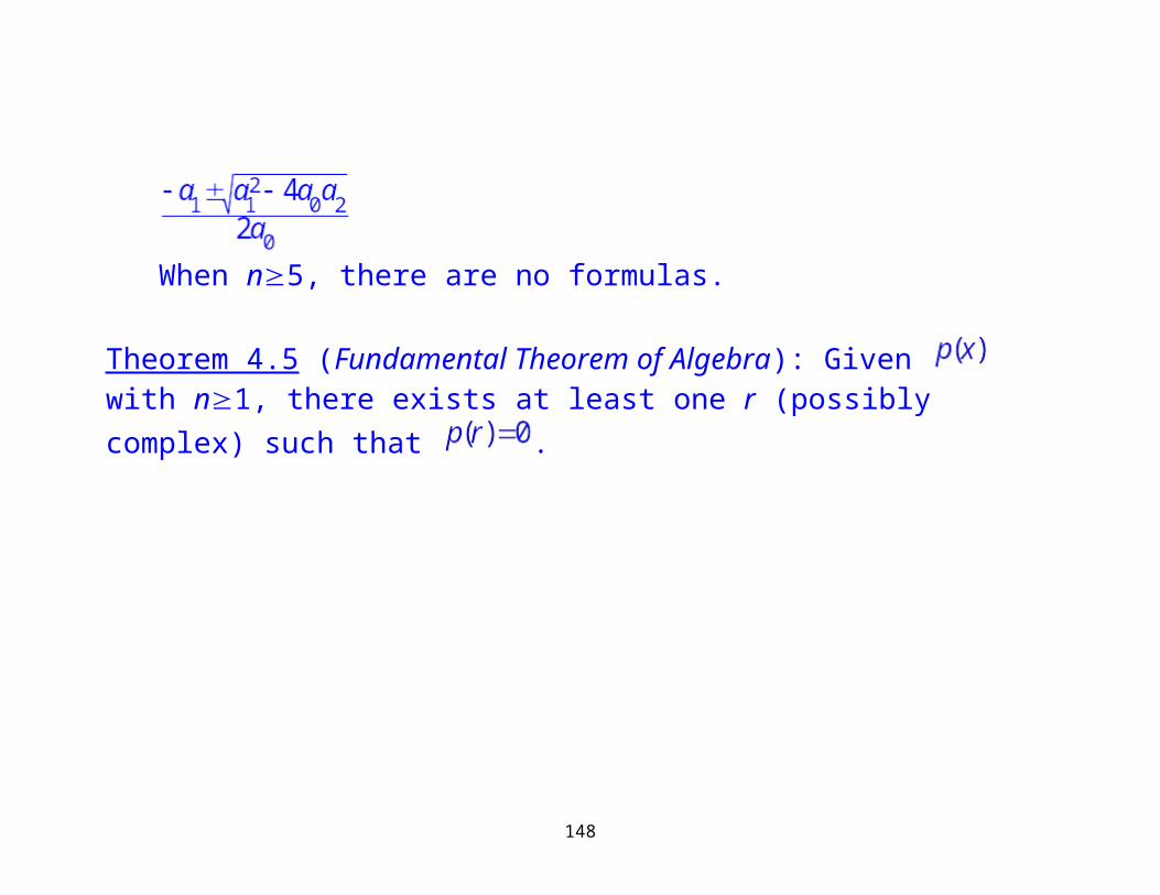
Properties: Computing and are easy. Finding zeroes when n4 is by use of formulas, e.g., when n=2,
When n5, there are no formulas.
Theorem 4.5 (Fundamental Theorem of Algebra): Given with n1, there exists at least one r (possibly complex) such that .
107
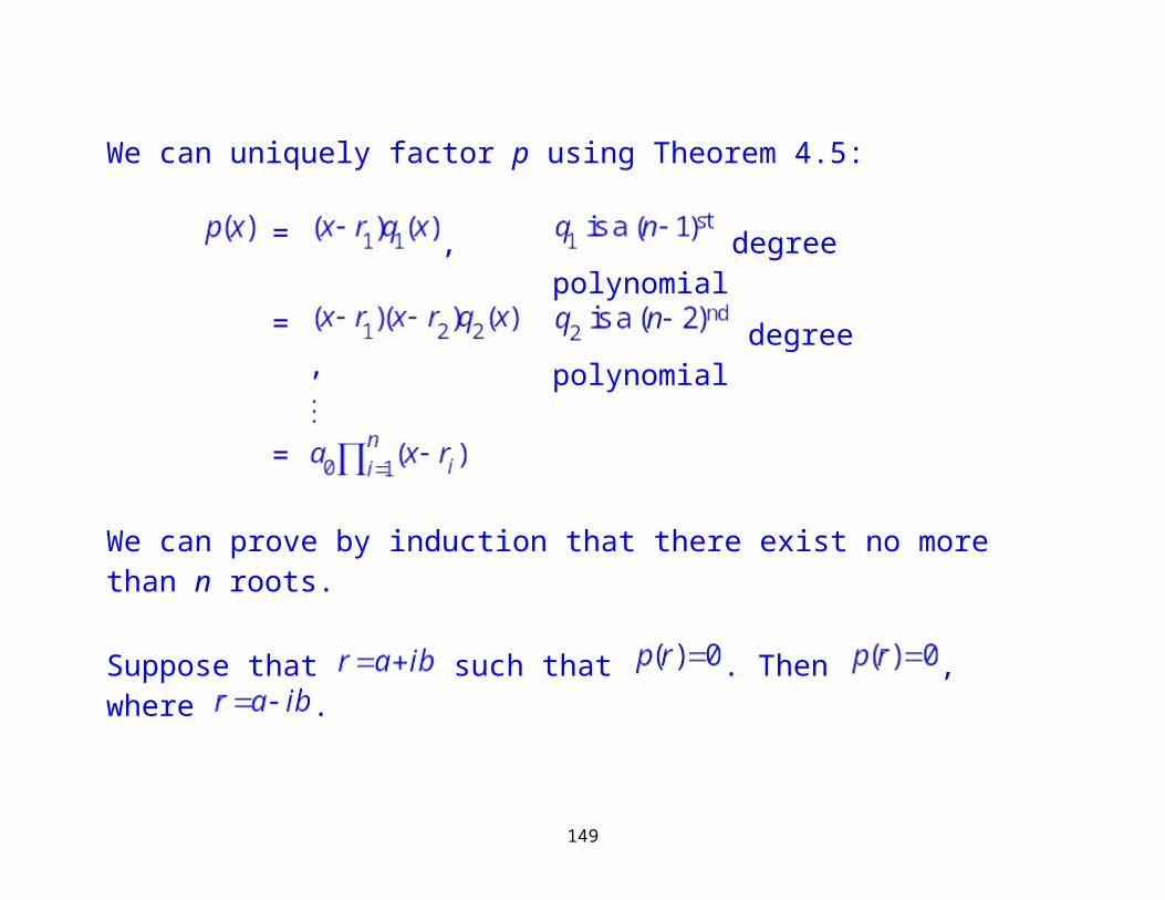
We can uniquely factor p using Theorem 4.5:
= , degree polynomial= , degree polynomial
=
We can prove by induction that there exist no more than n roots.
Suppose that such that . Then , where .
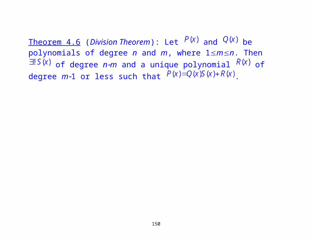
Theorem 4.6 (Division Theorem): Let and be polynomials of degree n and m, where 1mn. Then of degree nm and a unique polynomial
of degree m1 or less such that .
108
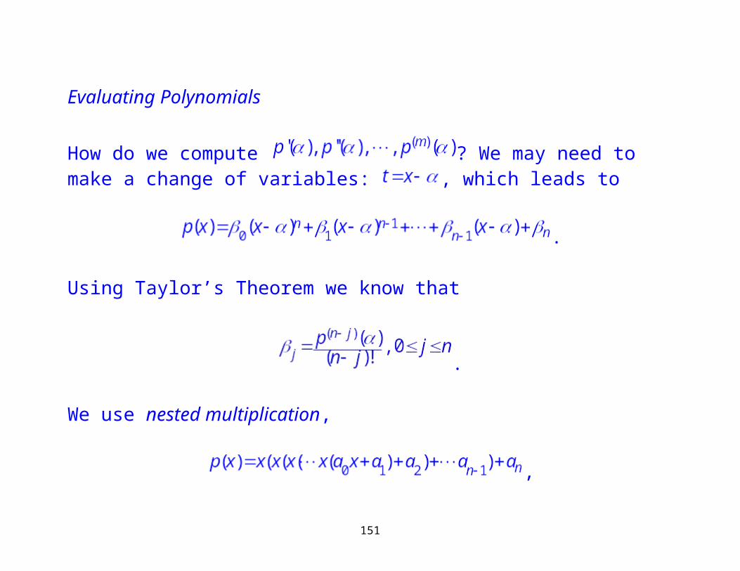
Evaluating Polynomials
How do we compute ? We may need to make a change of variables: , which leads to
.
Using Taylor’s Theorem we know that
.
We use nested multiplication,
,
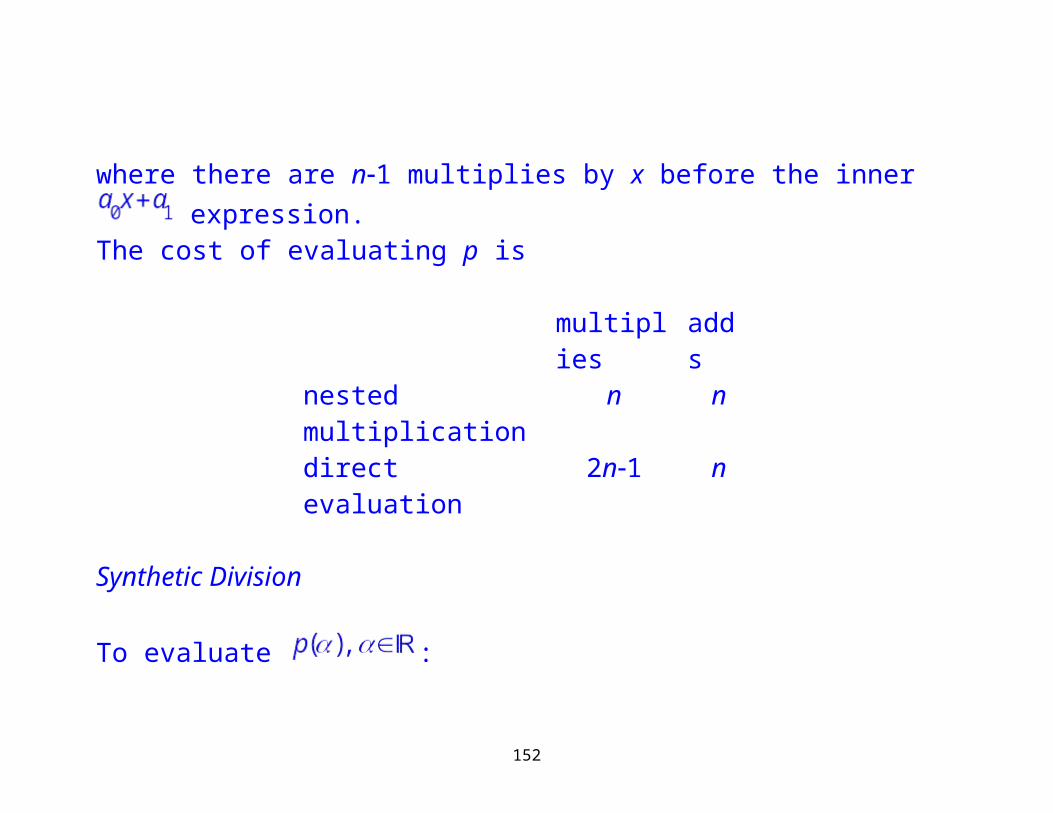
where there are n1 multiplies by x before the inner expression.
109
The cost of evaluating p is
multiplies addsnested multiplication n ndirect evaluation 2n1 n
Synthetic Division
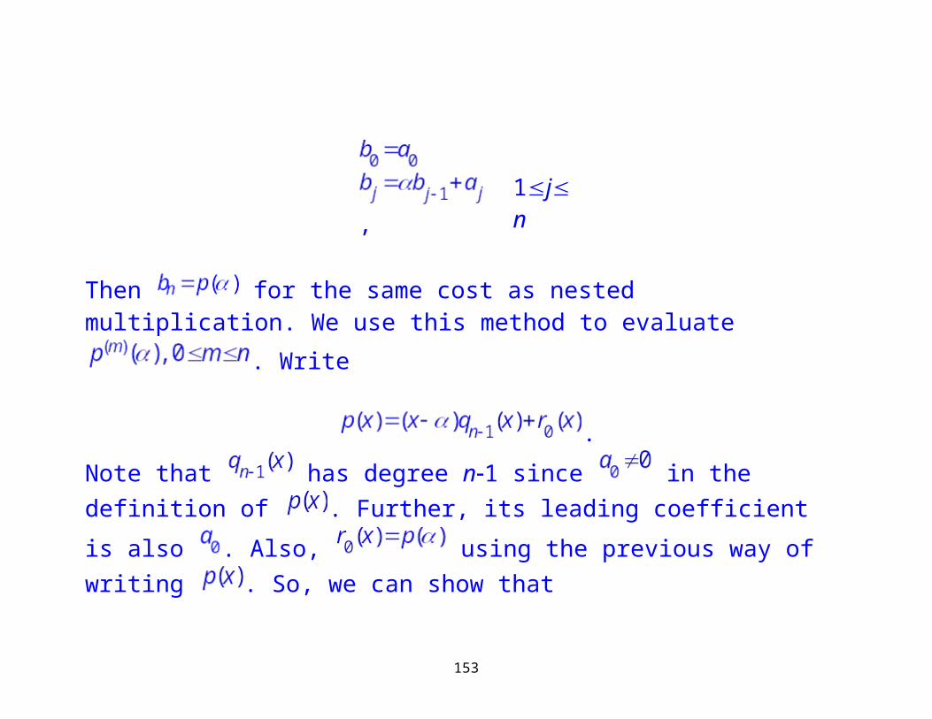
To evaluate :
, 1jn
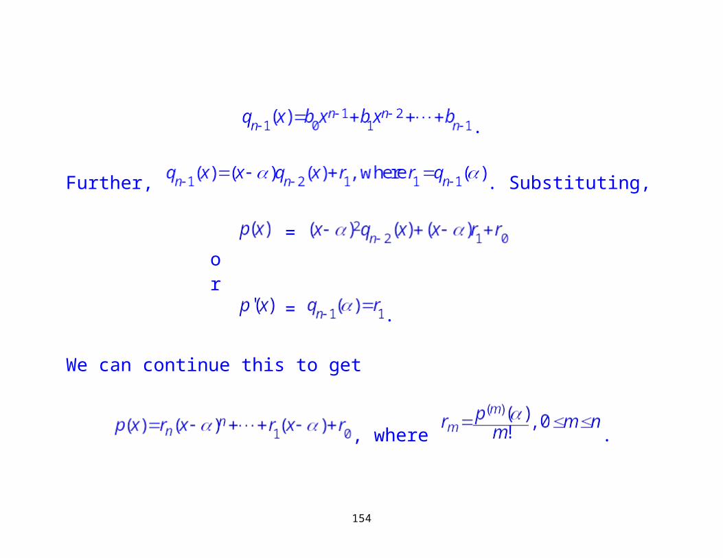
Then for the same cost as nested multiplication. We use this method to evaluate . Write
110
.
Note that has degree n1 since in the definition of . Further,
its leading coefficient is also . Also, using the previous way of writing . So, we can show that
.
Further, . Substituting,
=or
= .
We can continue this to get
111

, where .
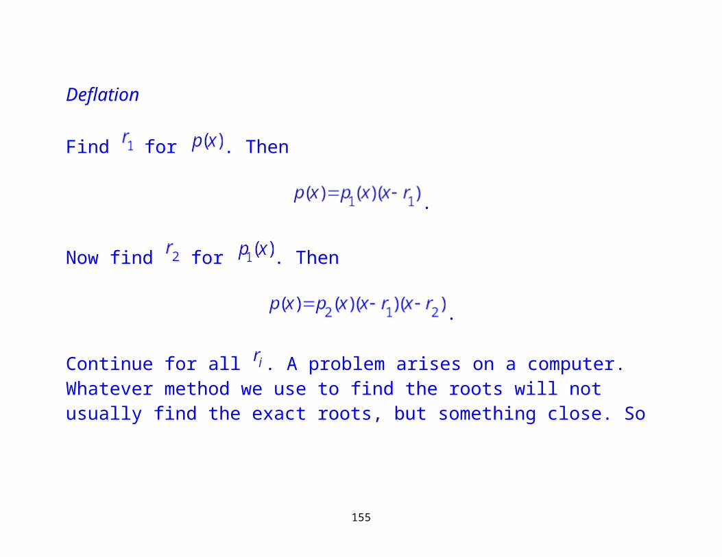
Deflation
Find for . Then
.
Now find for . Then
.
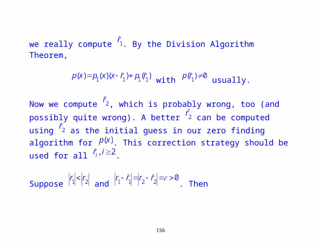
Continue for all . A problem arises on a computer. Whatever method we use to find the roots will not usually find the exact roots, but something close. So we really compute . By the Division Algorithm Theorem,
112
with usually.
Now we compute , which is probably wrong, too (and possibly quite wrong). A better can be computed using as the initial guess in our zero finding algorithm for . This correction strategy should be used for all .
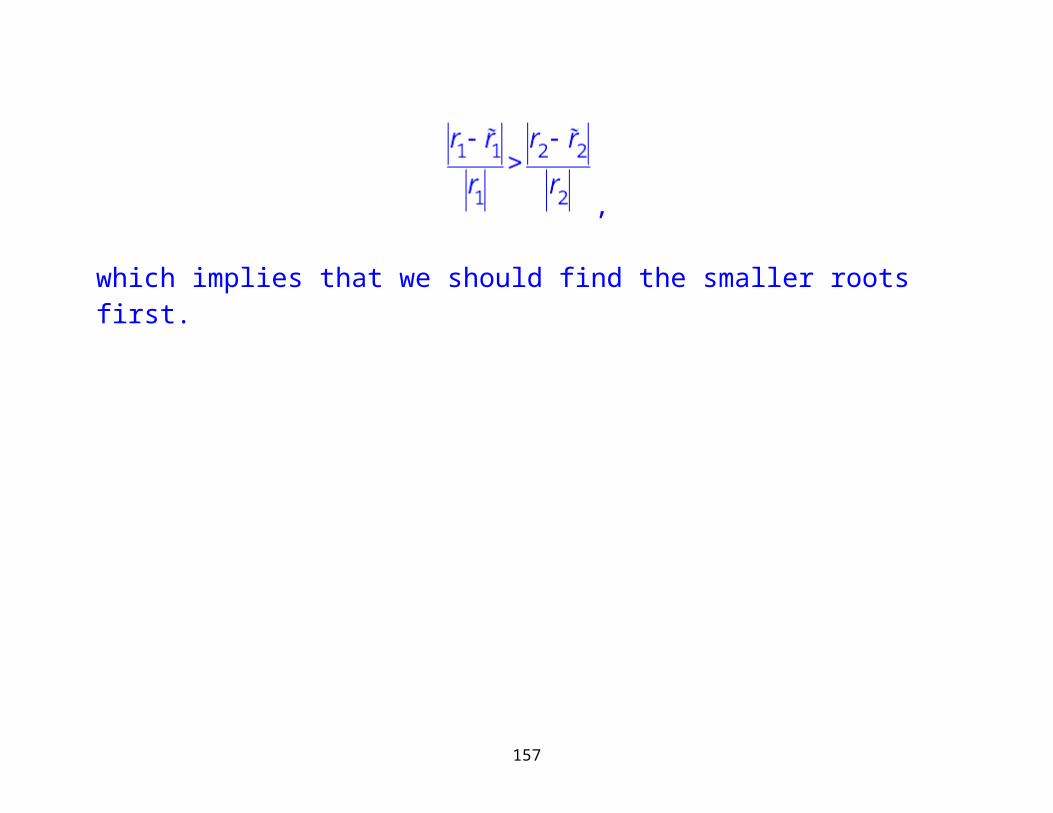
Suppose and . Then
,
which implies that we should find the smaller roots first.
113
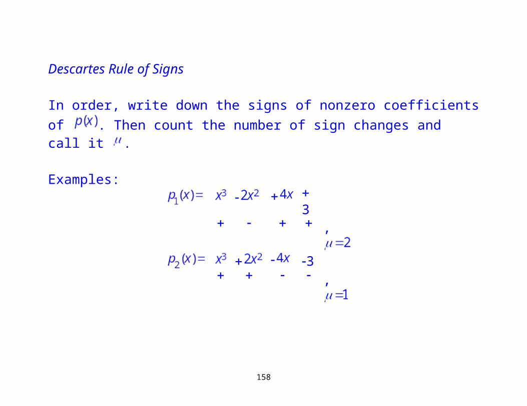
Descartes Rule of Signs
In order, write down the signs of nonzero coefficients of . Then count the number of sign changes and call it .
Examples:
3 ,
3 ,
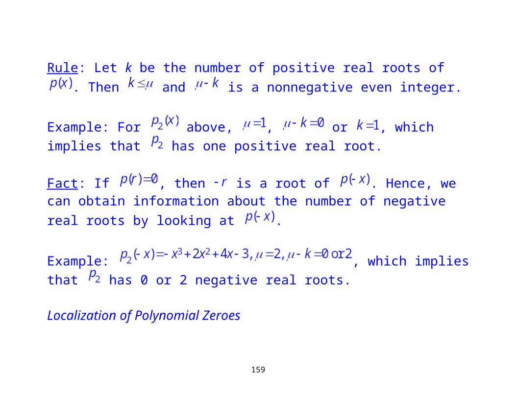
Rule: Let k be the number of positive real roots of . Then and is a nonnegative even integer.
Example: For above, , or , which implies that has one positive real root.
114
Fact: If , then is a root of . Hence, we can obtain information about the number of negative real roots by looking at .
Example: , which implies that has 0 or 2 negative real roots.
Localization of Polynomial Zeroes
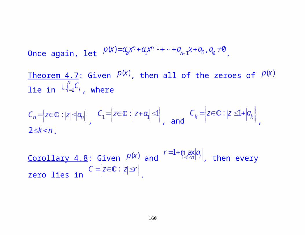
Once again, let .
Theorem 4.7: Given , then all of the zeroes of lie in , where
, , and , .
115
Corollary 4.8: Given and , then every zero lies in
.
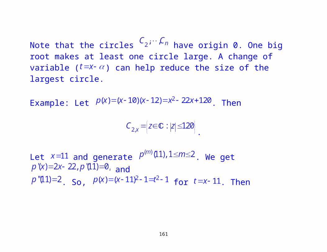
Note that the circles have origin 0. One big root makes at least one circle large. A change of variable ( ) can help reduce the size of the largest circle.
Example: Let . Then
.
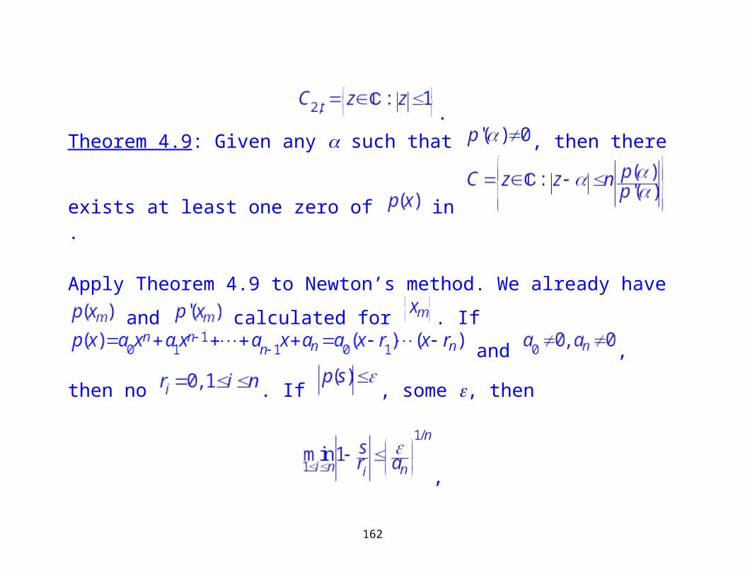
Let and generate . We get and . So, for . Then
116
.Theorem 4.9: Given any such that , then there exists at least one zero
of in .
Apply Theorem 4.9 to Newton’s method. We already have and
calculated for . If and
, then no . If , some , then
,
which is an upper bound on the relative error of s with respect to some zero of .
117
118
5. Interpolation and Approximation
Assume we want to approximate some function by a simpler function .
Example: a Taylor expansion.
Besides approximating , may be used to approximate or
.
Polynomial interpolation
. Most of the theory relies on
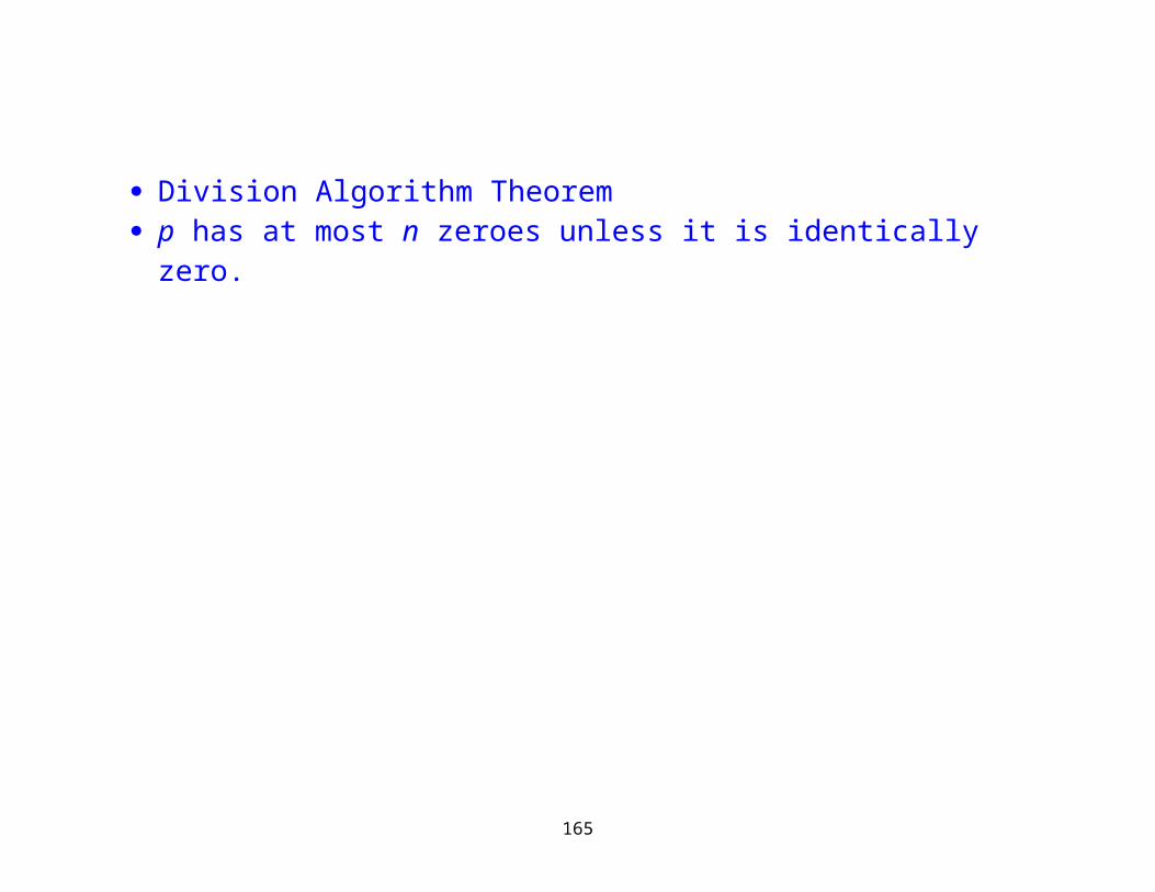
Division Algorithm Theorem p has at most n zeroes unless it is identically zero.
119
Lagrange interpolation
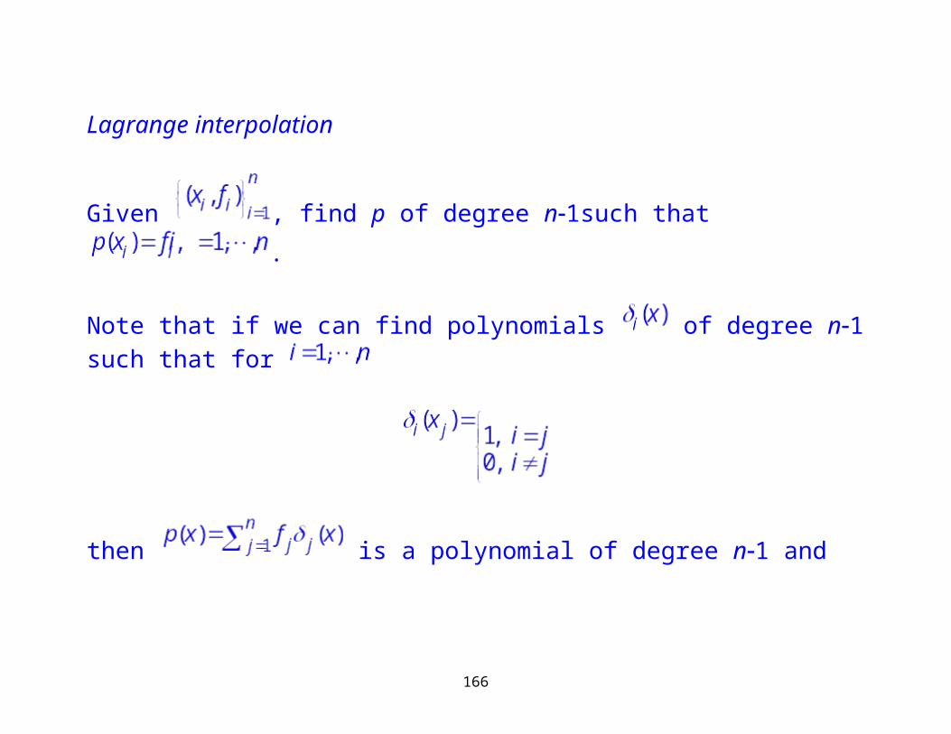
Given , find p of degree n1such that .
Note that if we can find polynomials of degree n1 such that for
then is a polynomial of degree n1 and
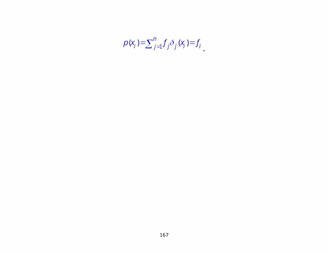
.
120
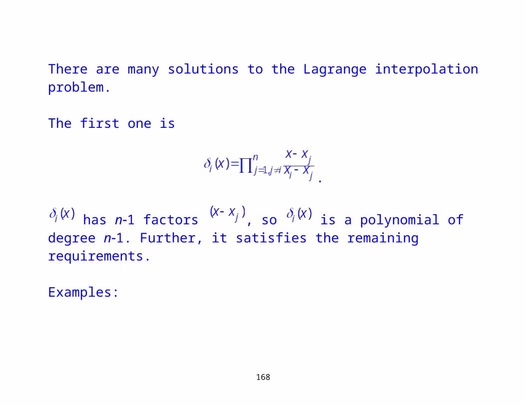
There are many solutions to the Lagrange interpolation problem.
The first one is
.
has n1 factors , so is a polynomial of degree n1. Further, it satisfies the remaining requirements.
Examples:
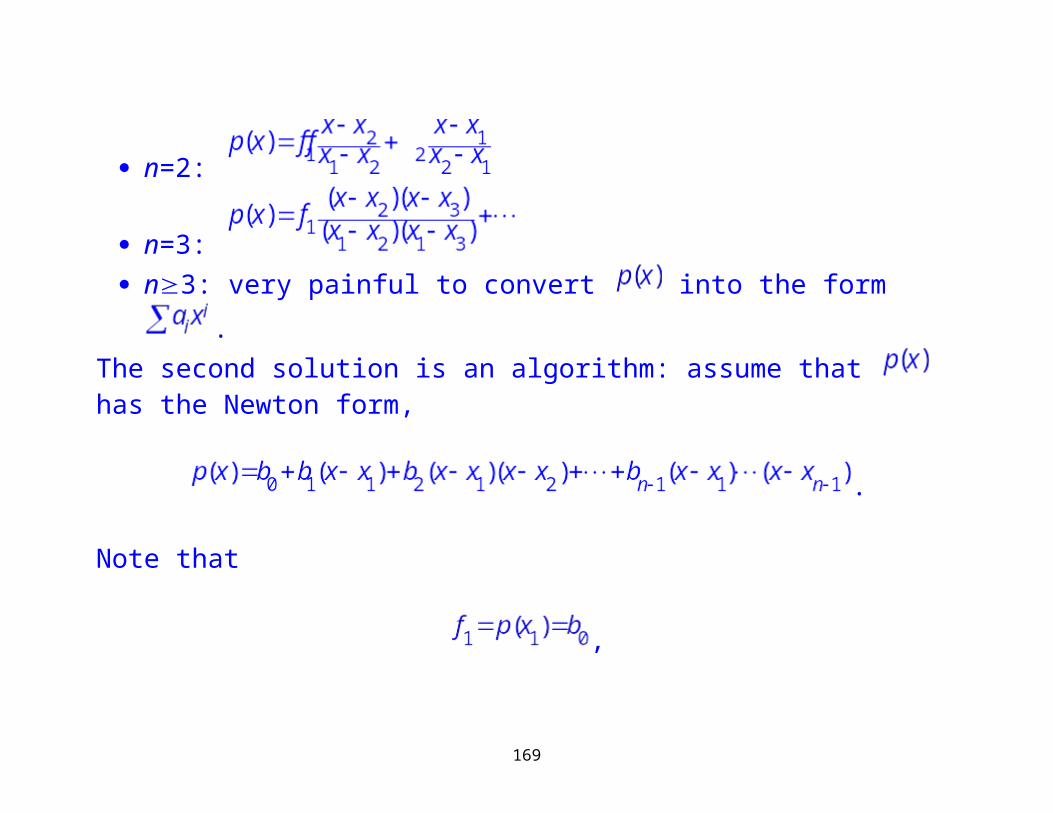
n=2:
n=3: n3: very painful to convert into the form .
121

The second solution is an algorithm: assume that has the Newton form,
.
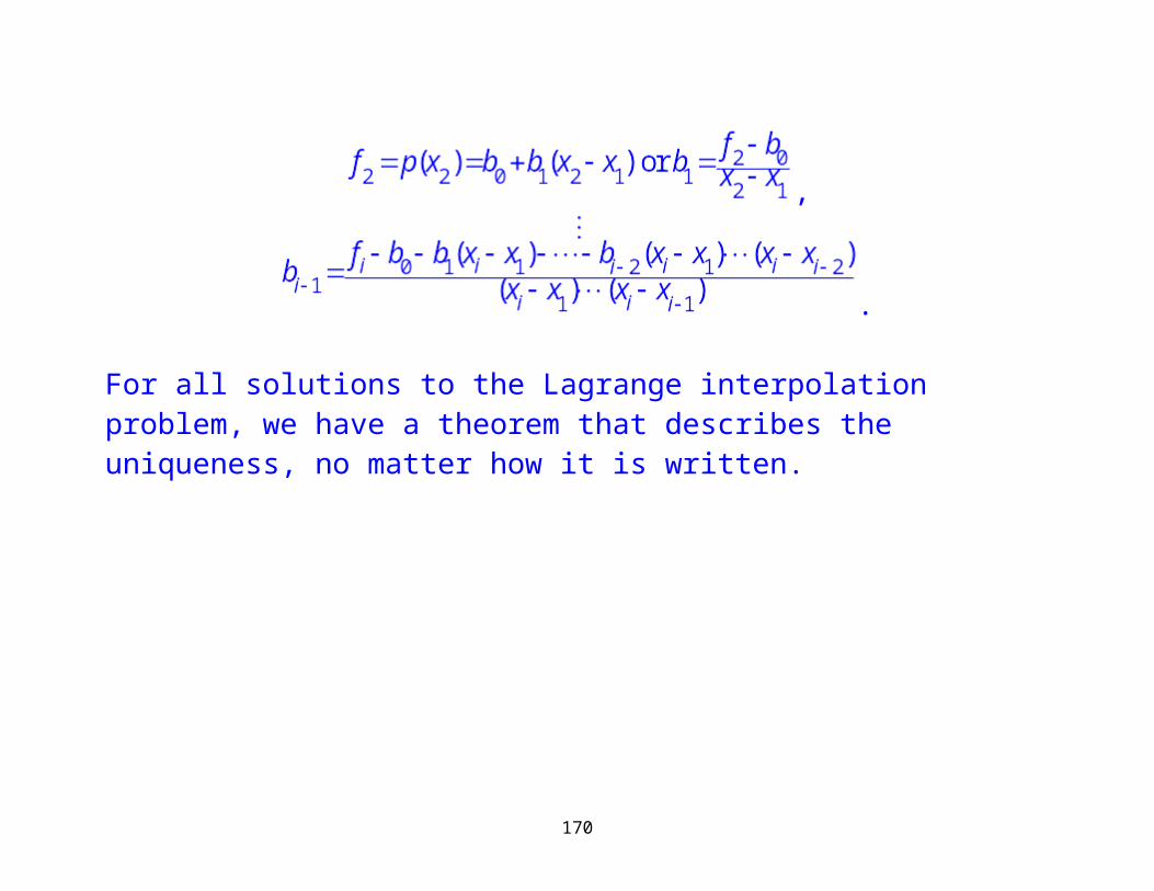
Note that
,
,
.
For all solutions to the Lagrange interpolation problem, we have a theorem that describes the uniqueness, no matter how it is written.
122
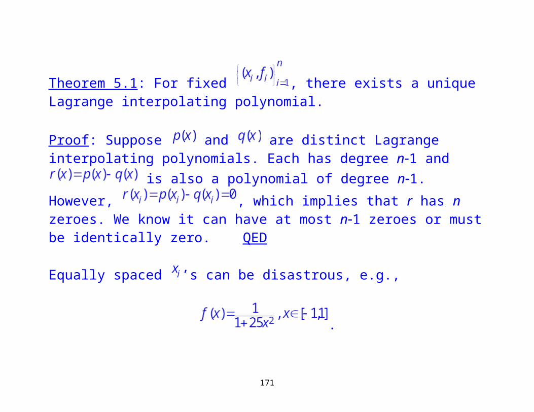
Theorem 5.1: For fixed , there exists a unique Lagrange interpolating polynomial.
Proof: Suppose and are distinct Lagrange interpolating polynomials. Each has degree n1 and is also a polynomial of degree n1. However, , which implies that r has n zeroes. We know it can have at most n1 zeroes or must be identically zero. QED
Equally spaced ’s can be disastrous, e.g.,
.
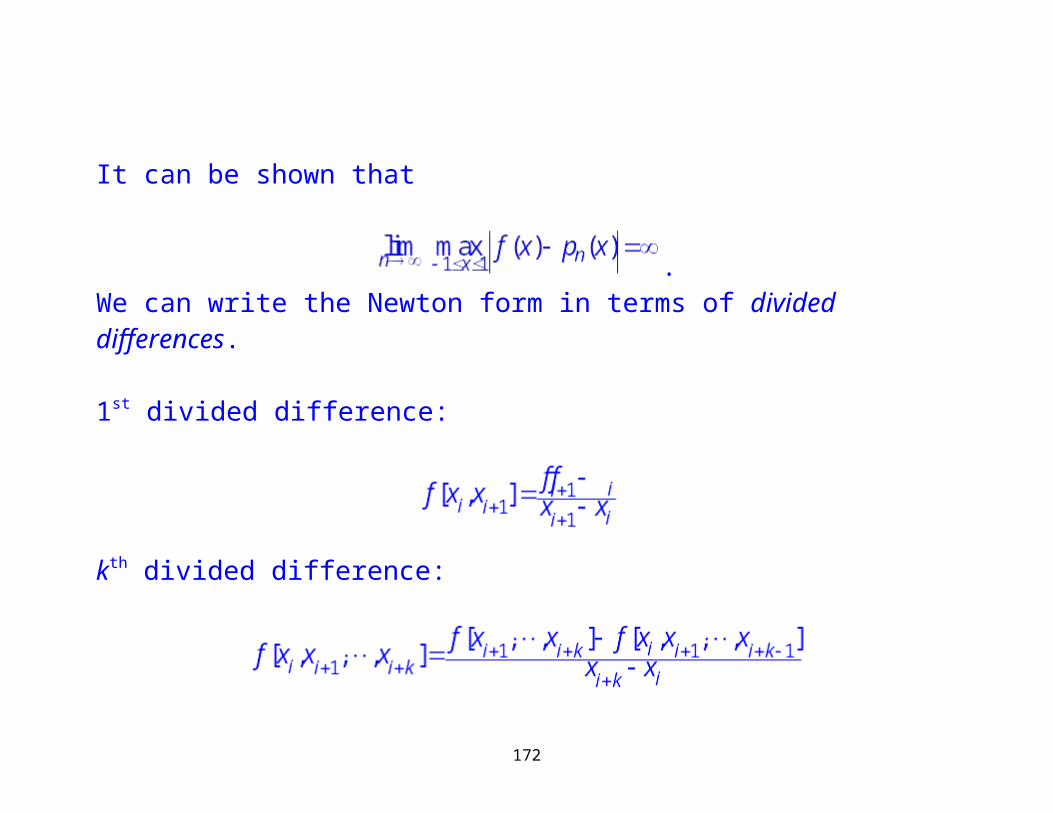
It can be shown that
.
123

We can write the Newton form in terms of divided differences.
1st divided difference:
kth divided difference:
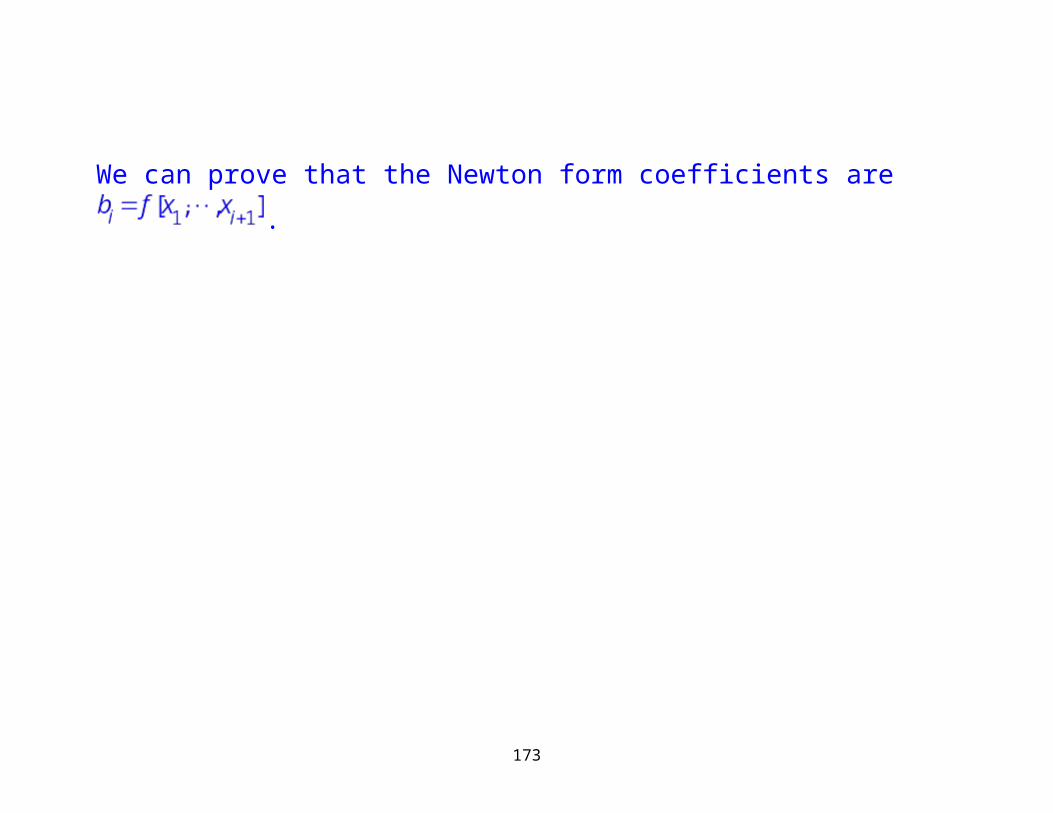
We can prove that the Newton form coefficients are .
124
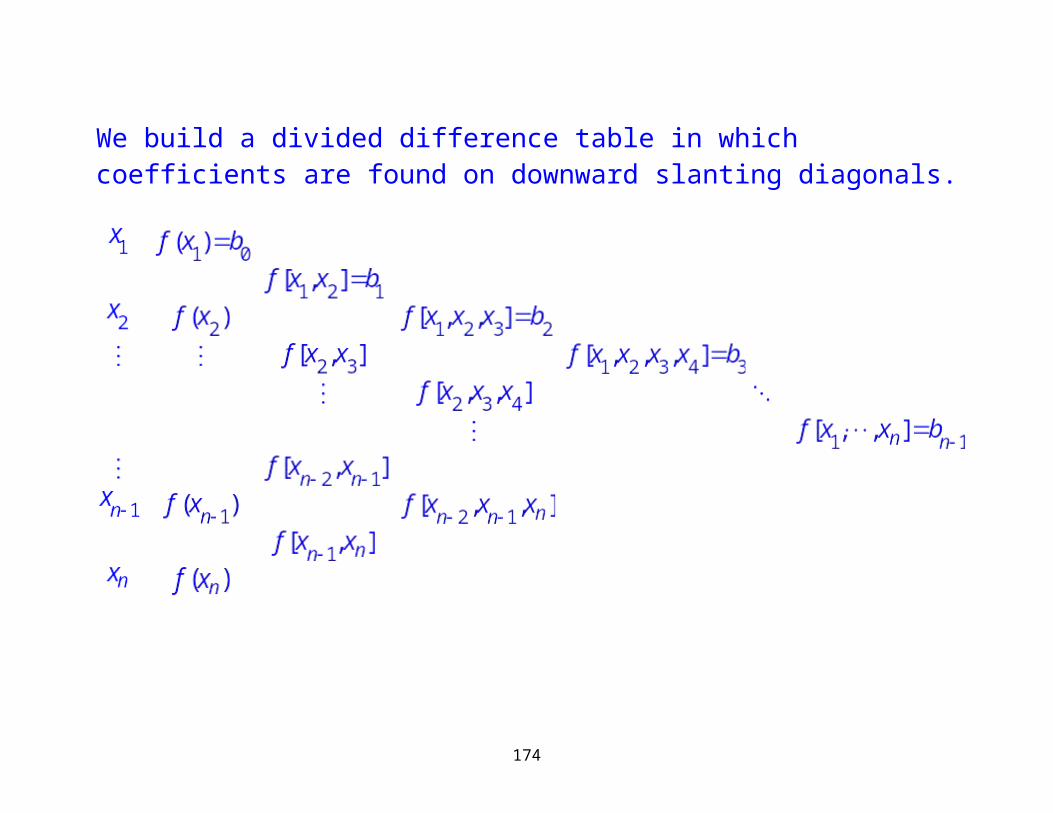
We build a divided difference table in which coefficients are found on downward slanting diagonals.
125
This table contains a wealth of information about many interpolating polynomials for . For example, the quadratic polynomial of at
is a table lookup starting at .
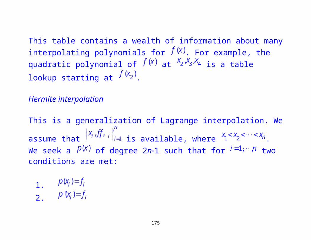
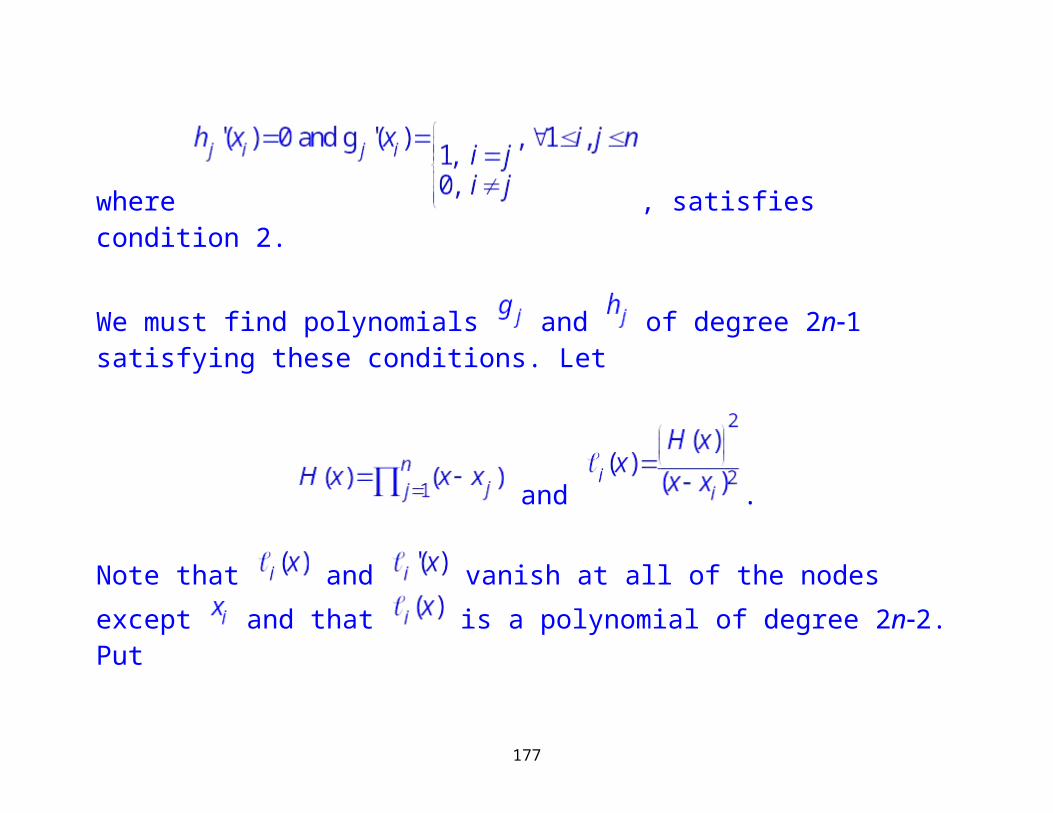
Hermite interpolation
This is a generalization of Lagrange interpolation. We assume that is available, where . We seek a of degree 2n1 such that for
two conditions are met:
1.2.
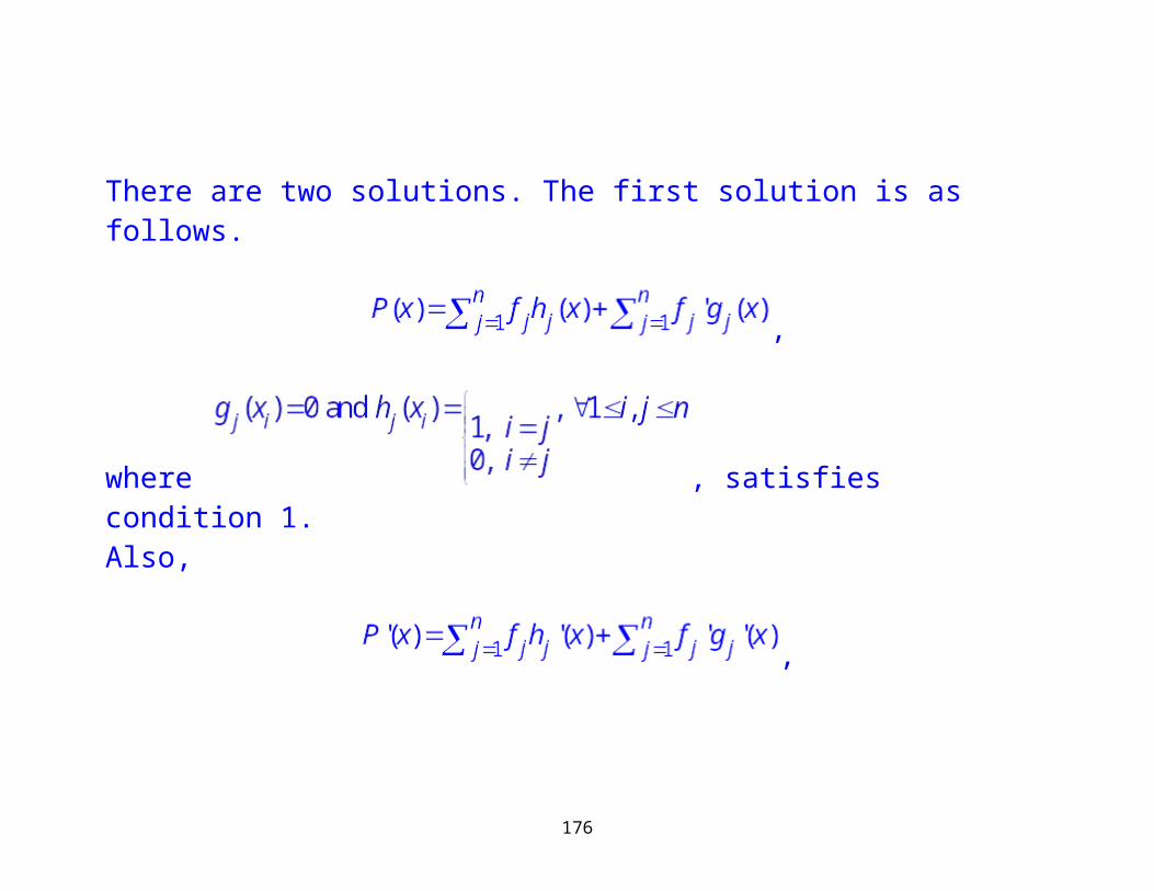
There are two solutions. The first solution is as follows.
126
,
where , satisfies condition 1.Also,
,
where , satisfies condition 2.
We must find polynomials and of degree 2n1 satisfying these conditions. Let
127
and .
Note that and vanish at all of the nodes except and that is a polynomial of degree 2n2. Put
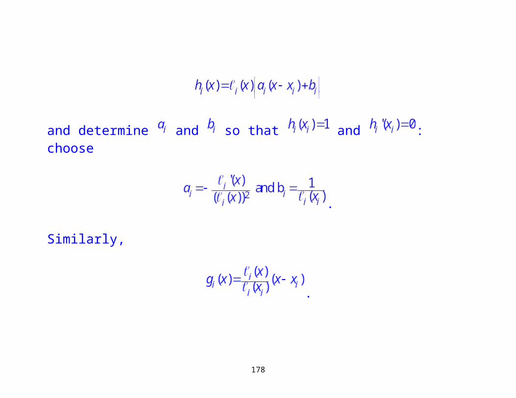
and determine and so that and : choose
.
Similarly,
128
.
129
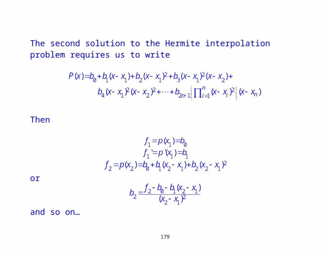
The second solution to the Hermite interpolation problem requires us to write
Then
or
and so on…
130
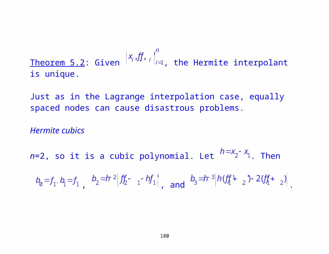
Theorem 5.2: Given , the Hermite interpolant is unique.
Just as in the Lagrange interpolation case, equally spaced nodes can cause disastrous problems.
Hermite cubics
n=2, so it is a cubic polynomial. Let . Then
, , and .
Hermite cubics is by far the most common form of Hermite interpolation that you are likely to see in practice.
131
Piecewise polynomial interpolation
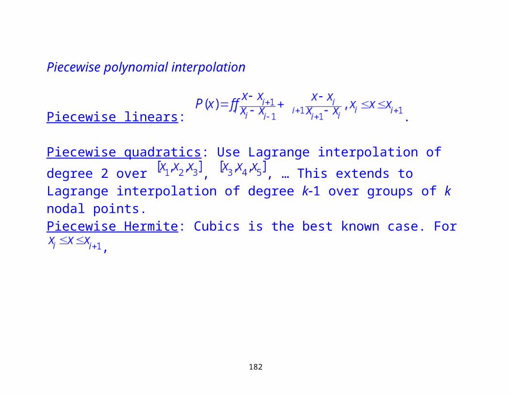
Piecewise linears: .
Piecewise quadratics: Use Lagrange interpolation of degree 2 over , , … This extends to Lagrange interpolation of degree k1 over groups
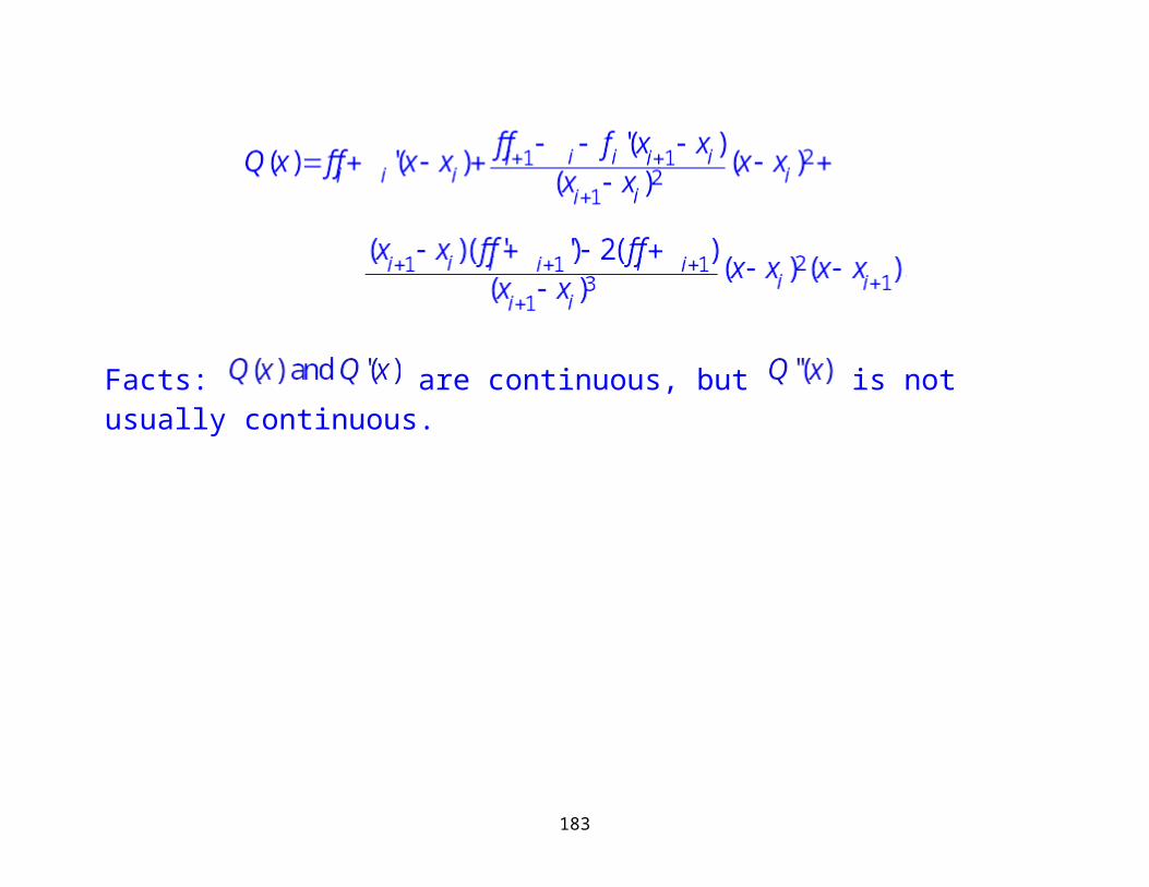
of k nodal points.Piecewise Hermite: Cubics is the best known case. For ,
132
Facts: are continuous, but is not usually continuous.
133
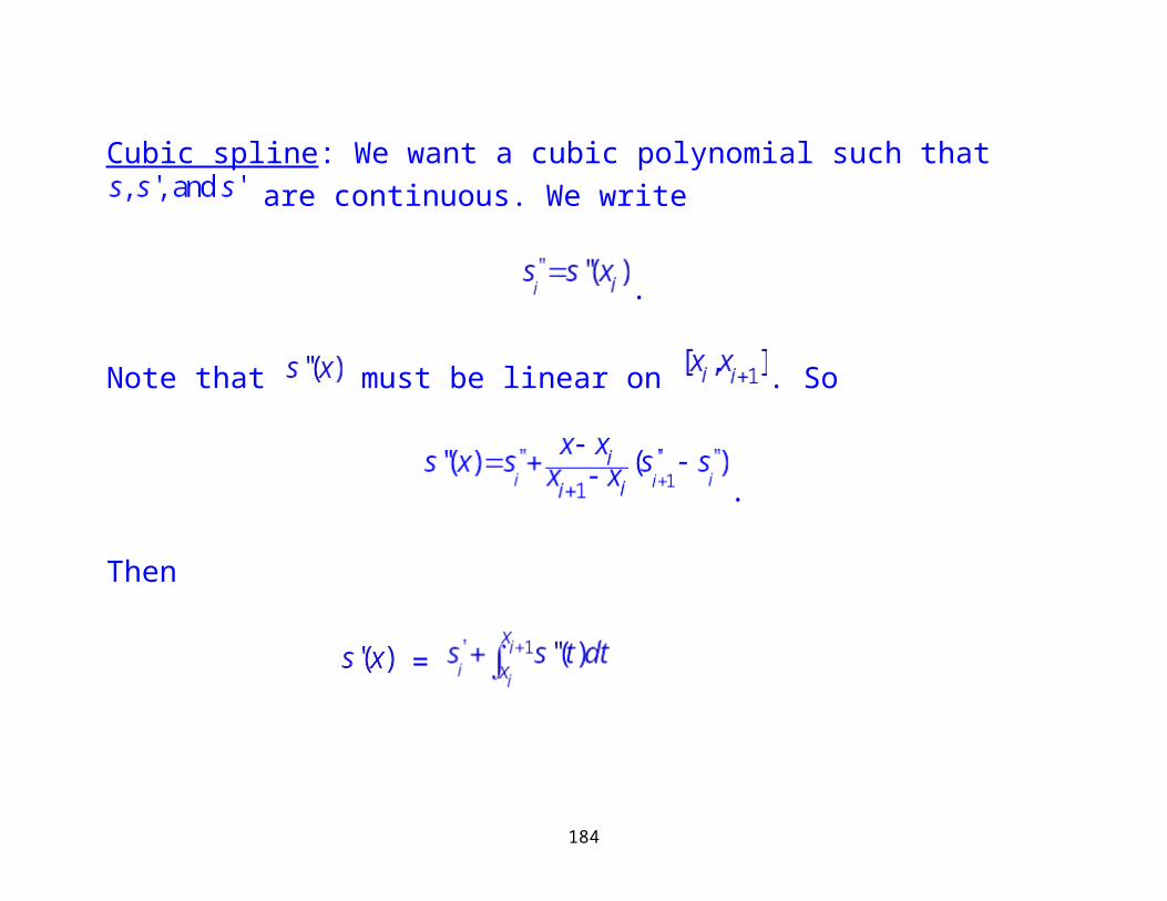
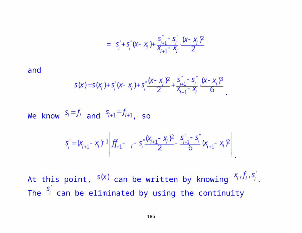
Cubic spline: We want a cubic polynomial such that are continuous. We write
.
Note that must be linear on . So
.
Then
=
=
134
and
.
We know and , so
.
At this point, can be written by knowing . The can be eliminated
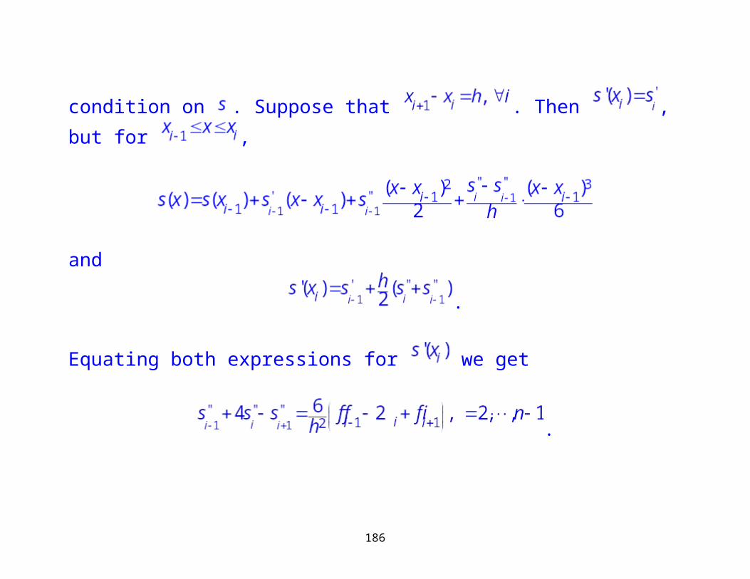
by using the continuity condition on . Suppose that . Then
, but for ,
135
and
.
Equating both expressions for we get
.
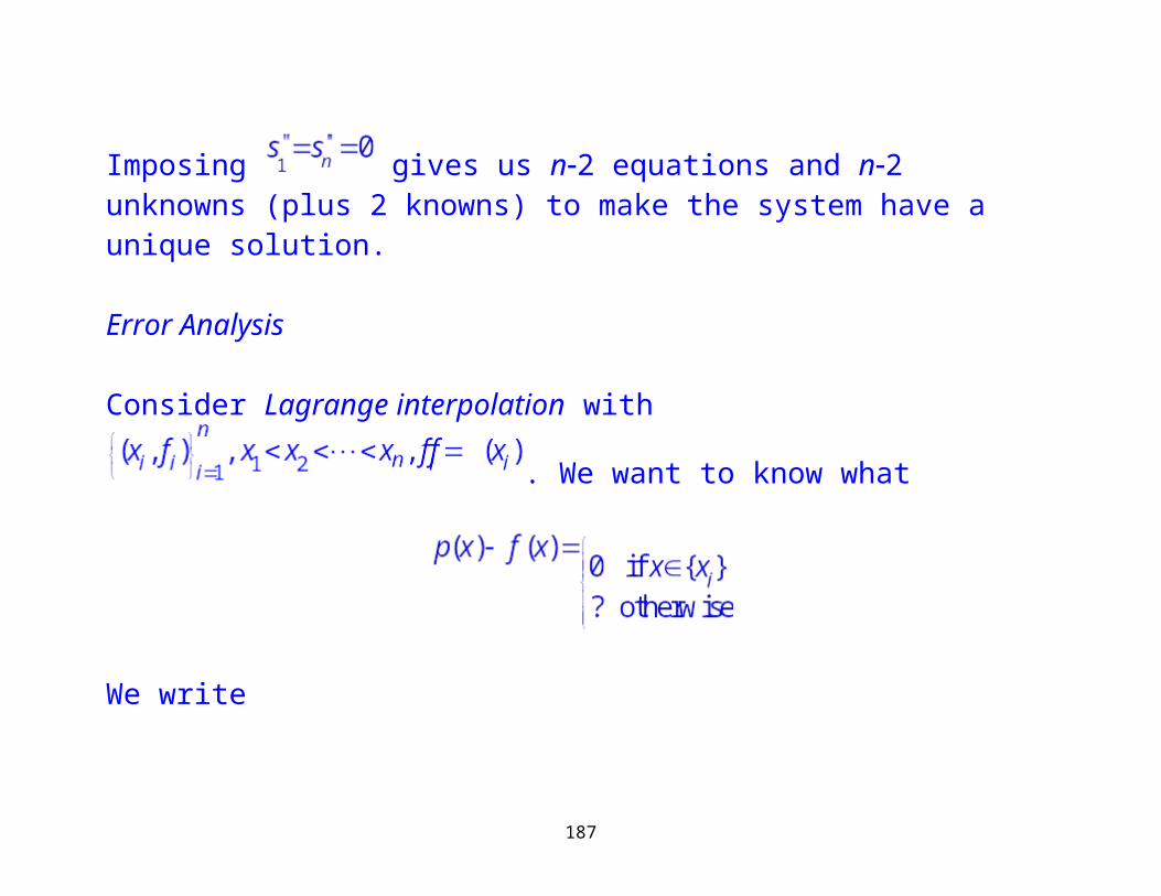
Imposing gives us n2 equations and n2 unknowns (plus 2 knowns) to make the system have a unique solution.
Error Analysis
Consider Lagrange interpolation with . We want to know what
136
We write
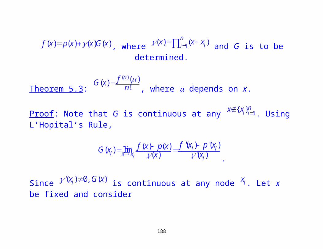
, where and G is to be determined.
Theorem 5.3: , where depends on x.
Proof: Note that G is continuous at any . Using L’Hopital’s Rule,
.
137
Since is continuous at any node . Let x be fixed and consider
.
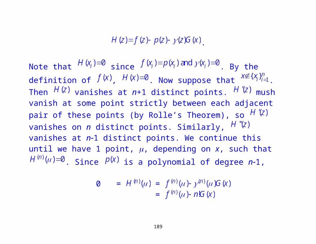
Note that since . By the definition of ,
. Now suppose that . Then vanishes at n+1 distinct points. mush vanish at some point strictly between each adjacent pair of these points (by Rolle’s Theorem), so vanishes on n distinct points. Similarly, vanishes at n1 distinct points. We continue this until we have 1 point, , depending on x, such that . Since is a polynomial of degree n1,
0 = ==
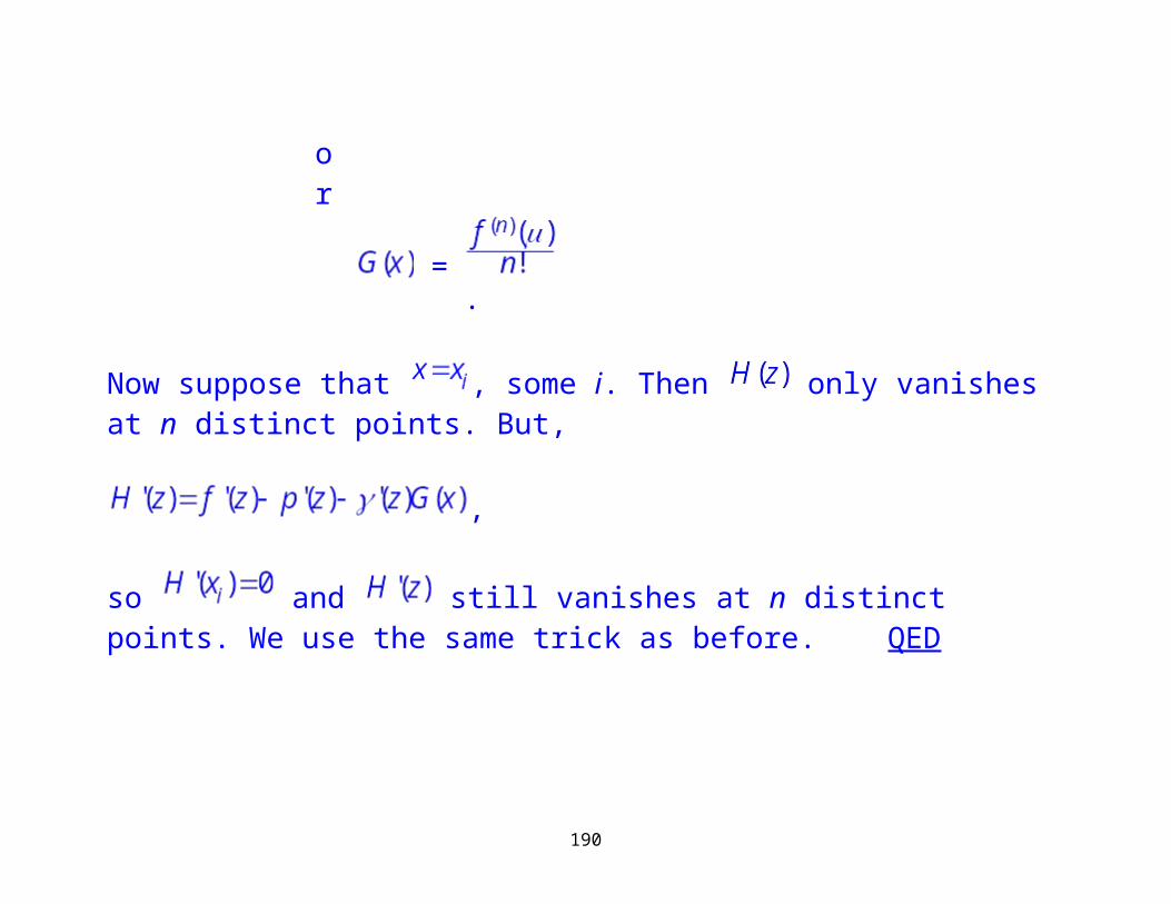
or
138
=.
Now suppose that , some i. Then only vanishes at n distinct points. But,
,
so and still vanishes at n distinct points. We use the same trick as before. QED
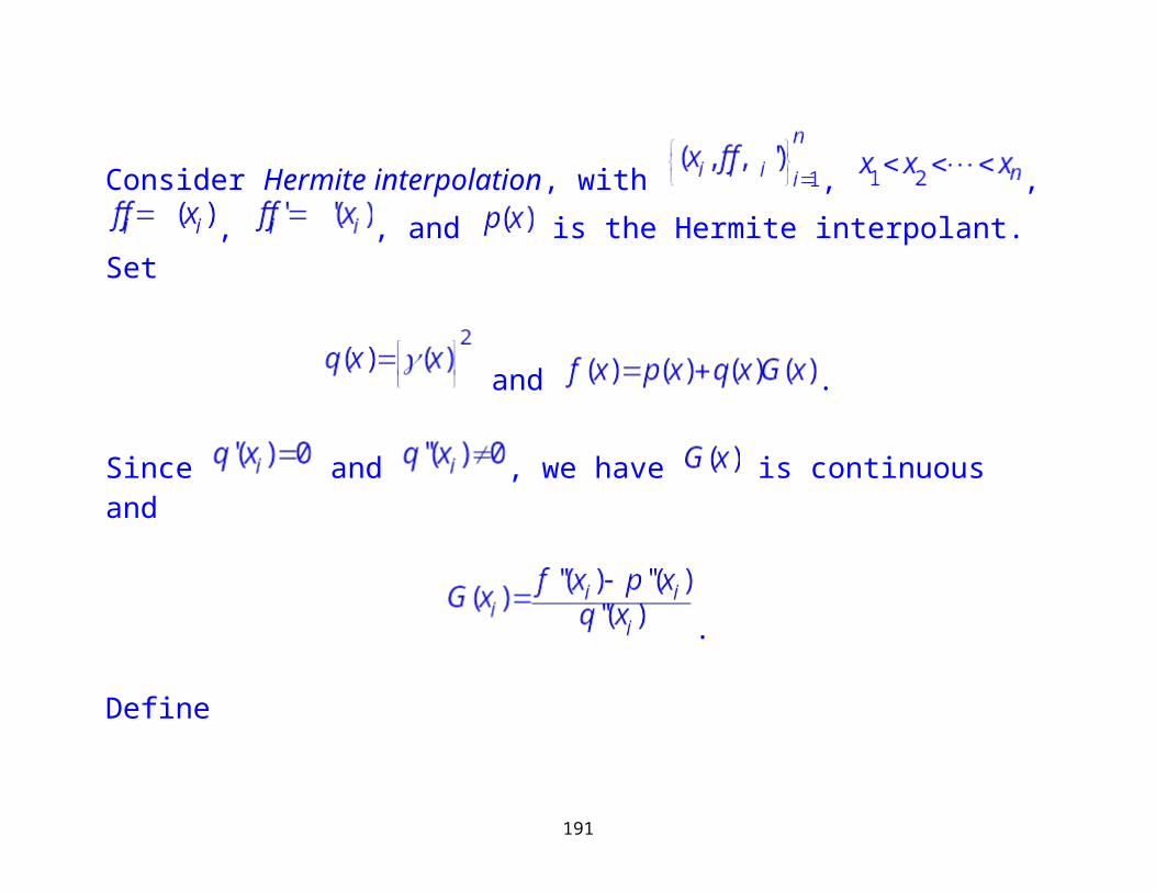
Consider Hermite interpolation, with , , , , and is the Hermite interpolant. Set
139

and .
Since and , we have is continuous and
.
Define
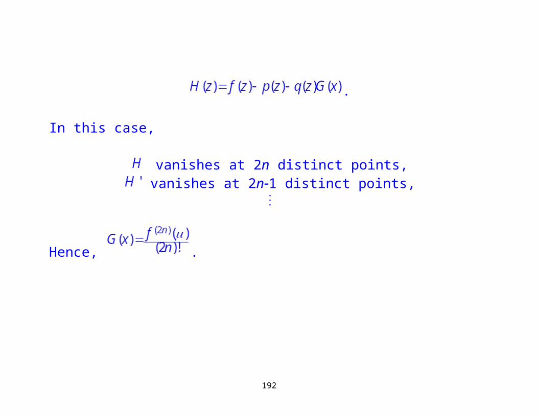
.
In this case,
vanishes at 2n distinct points, vanishes at 2n1 distinct points,
140
Hence, .
141

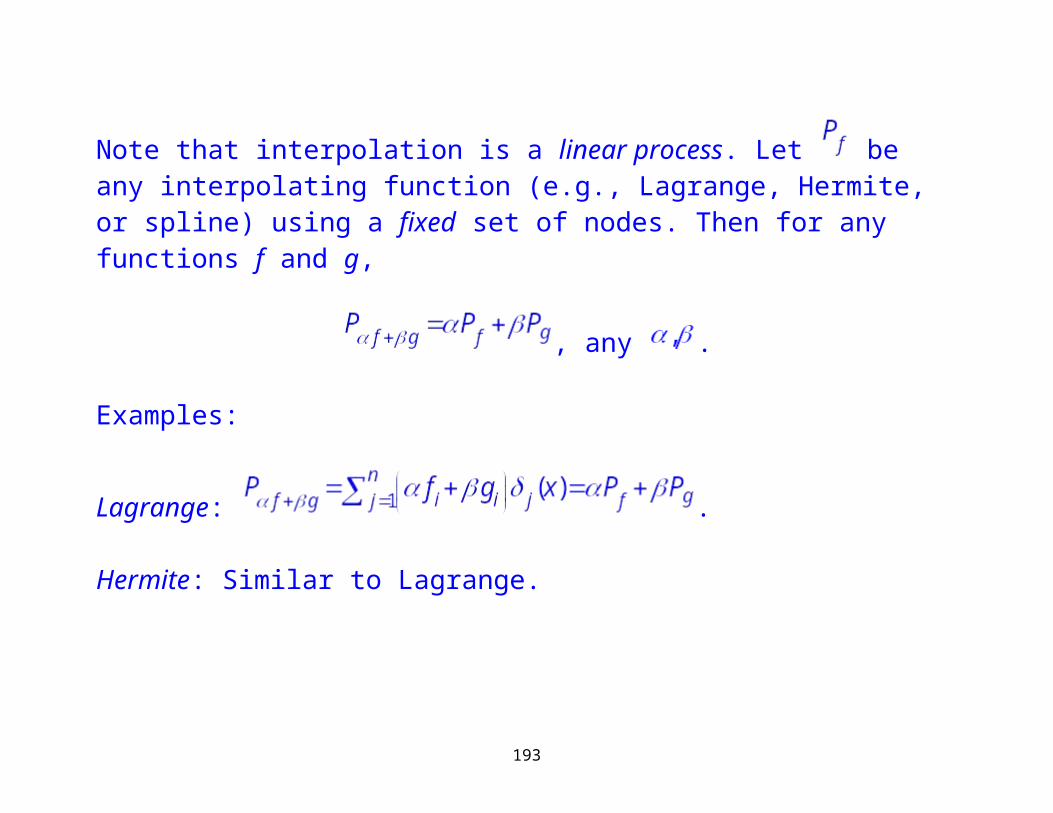
Note that interpolation is a linear process. Let be any interpolating function (e.g., Lagrange, Hermite, or spline) using a fixed set of nodes. Then for any functions f and g,
, any .
Examples:
Lagrange: .
Hermite: Similar to Lagrange.
142
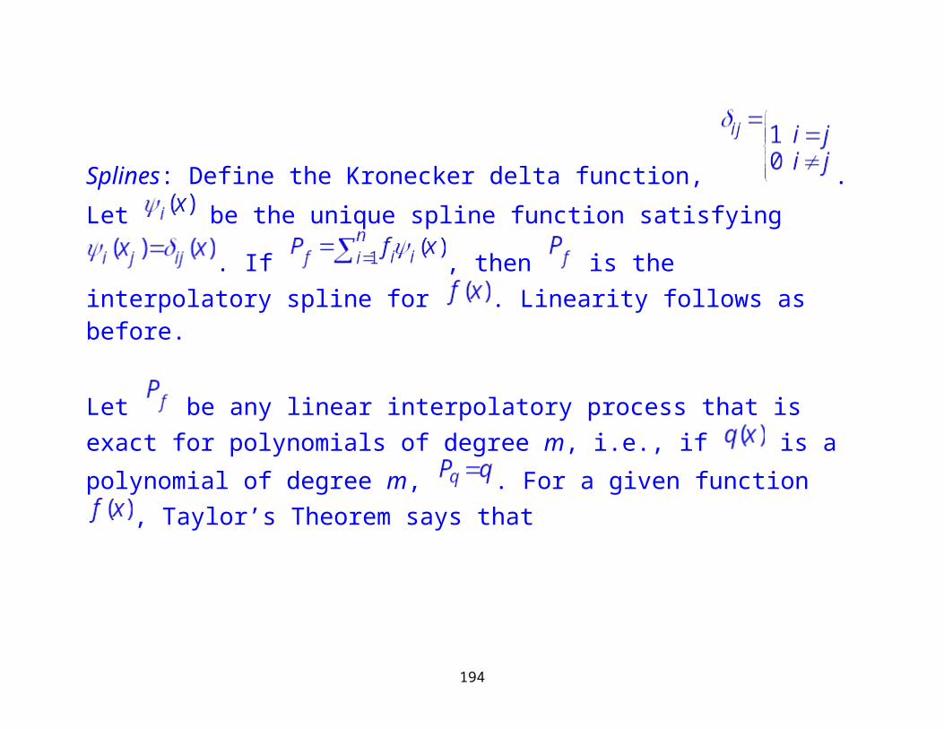
Splines: Define the Kronecker delta function, . Let be the
unique spline function satisfying . If , then is the interpolatory spline for . Linearity follows as before.
Let be any linear interpolatory process that is exact for polynomials of degree m, i.e., if is a polynomial of degree m, . For a given function
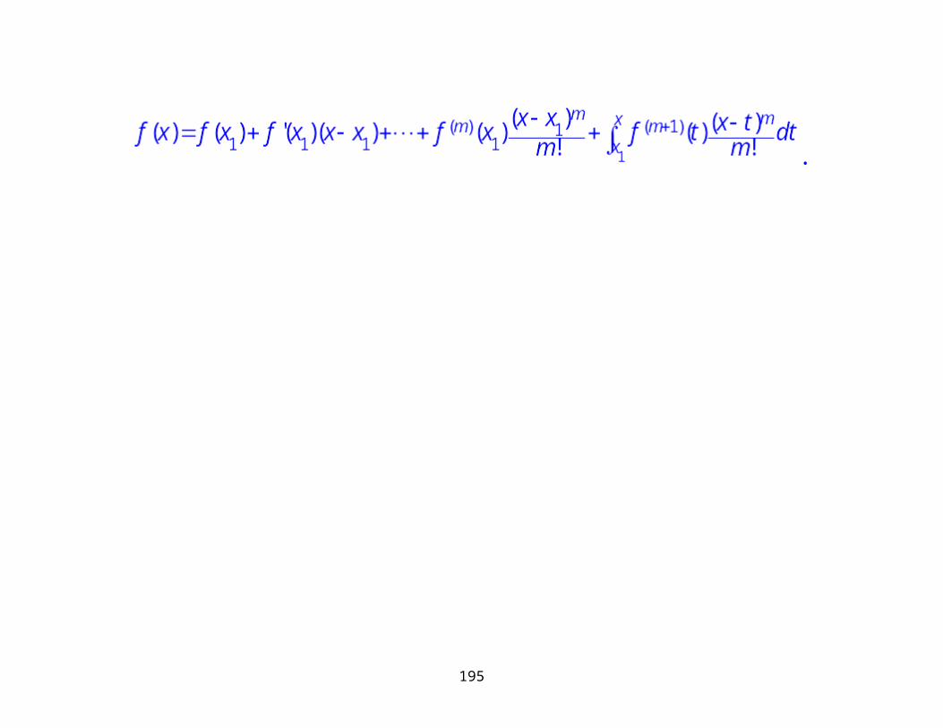
, Taylor’s Theorem says that
.
143
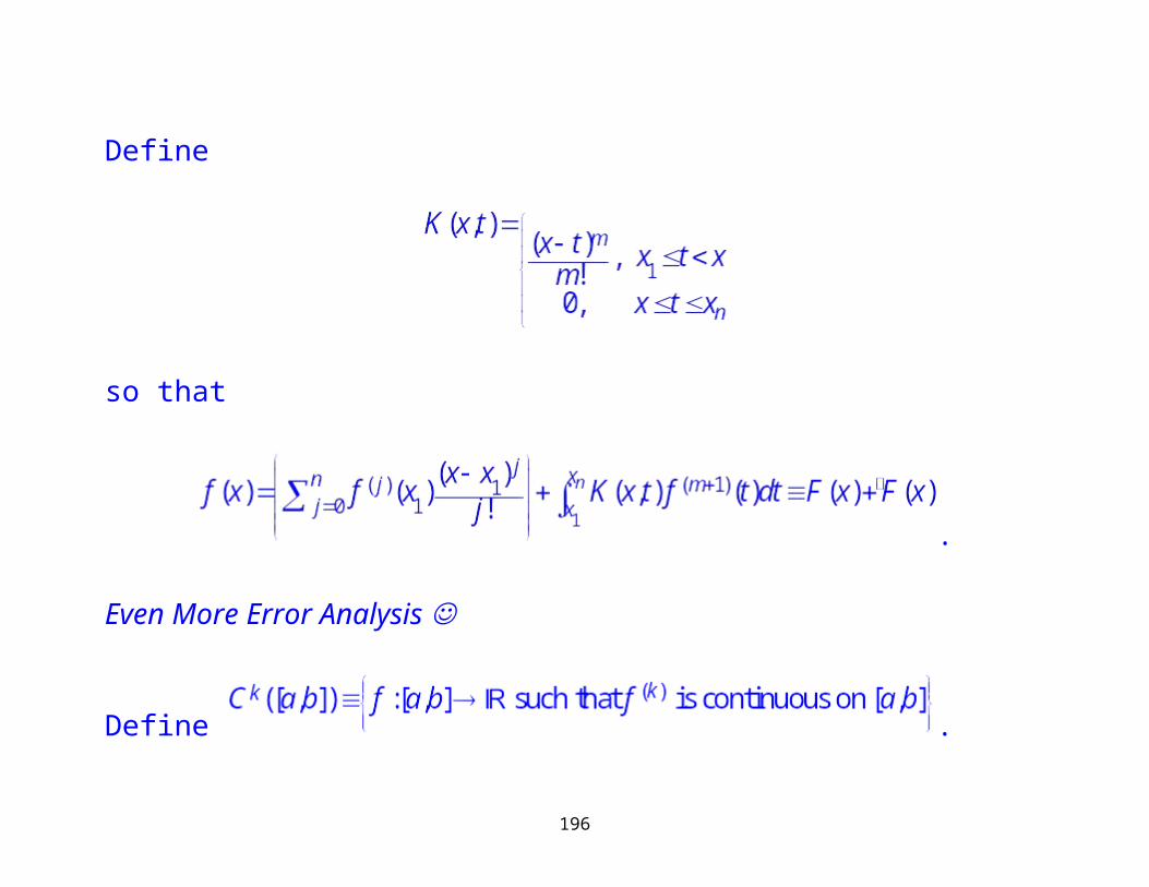
Define
so that
.
Even More Error Analysis
Define .
144
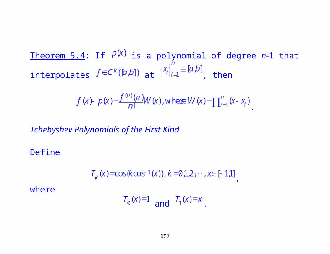
Theorem 5.4: If is a polynomial of degree n1 that interpolates
at , then
.
Tchebyshev Polynomials of the First Kind
Define
,where
and .
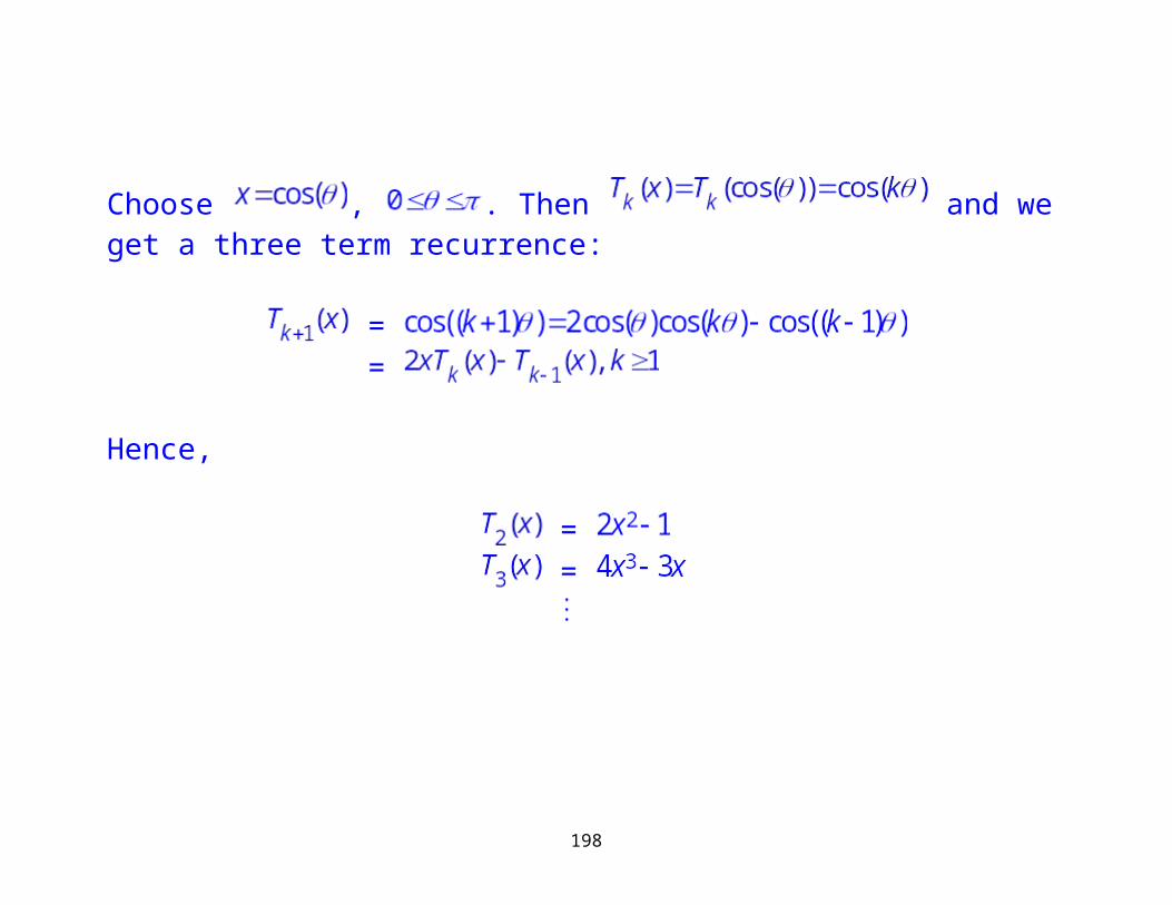
Choose , . Then and we get a three term recurrence:
145
==
Hence,
==
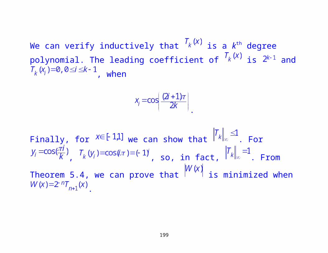
We can verify inductively that is a kth degree polynomial. The leading
coefficient of is and , when
.
146
Finally, for we can show that . For ,
, so, in fact, . From Theorem 5.4, we can prove that
is minimized when .
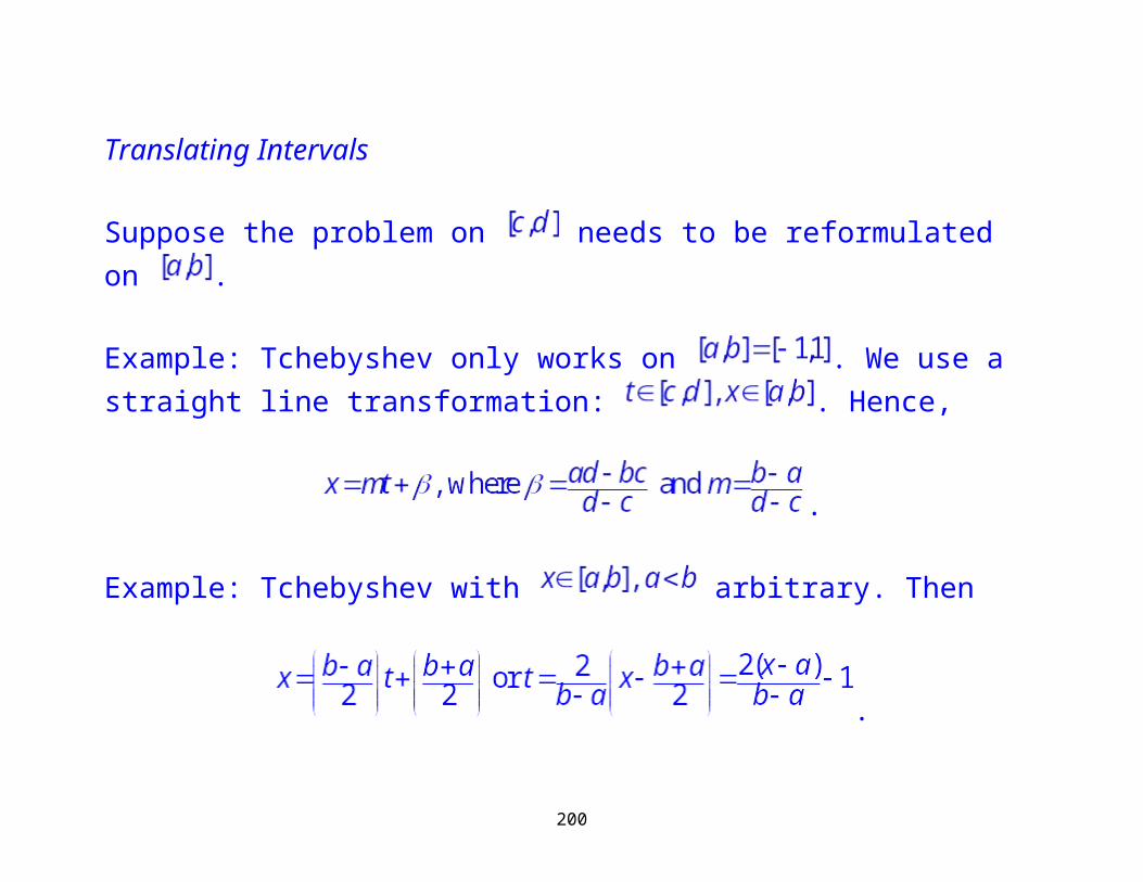
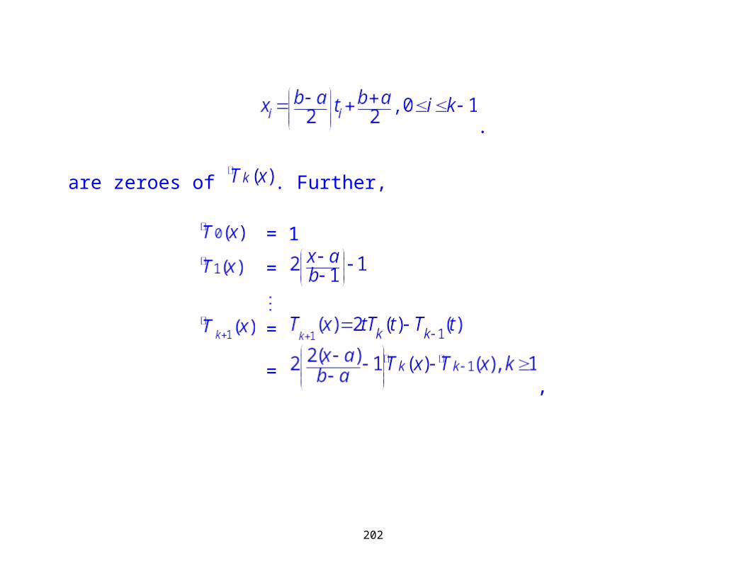
Translating Intervals
Suppose the problem on needs to be reformulated on .
Example: Tchebyshev only works on . We use a straight line transformation: . Hence,
.
Example: Tchebyshev with arbitrary. Then
147
.
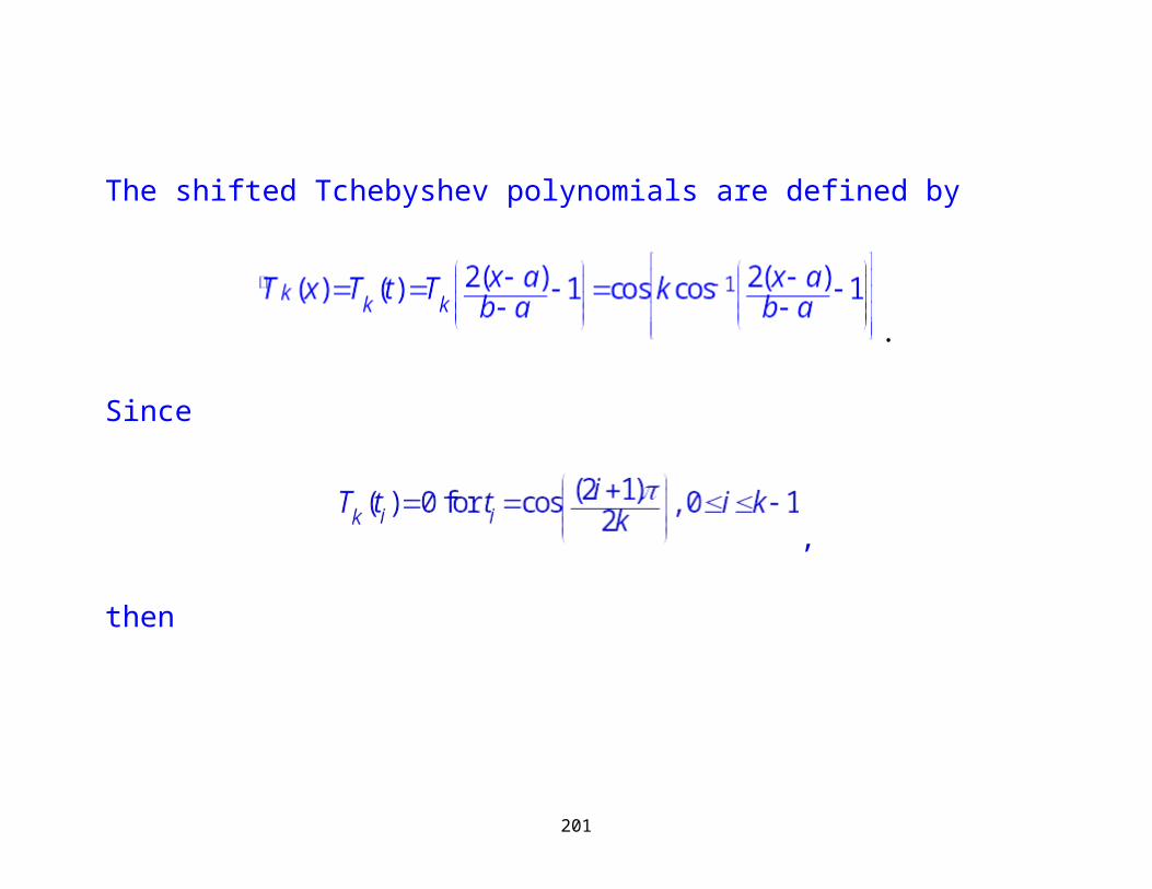
The shifted Tchebyshev polynomials are defined by
.
Since
,
then
148
.
are zeroes of . Further,
= 1
=
=
=,
149
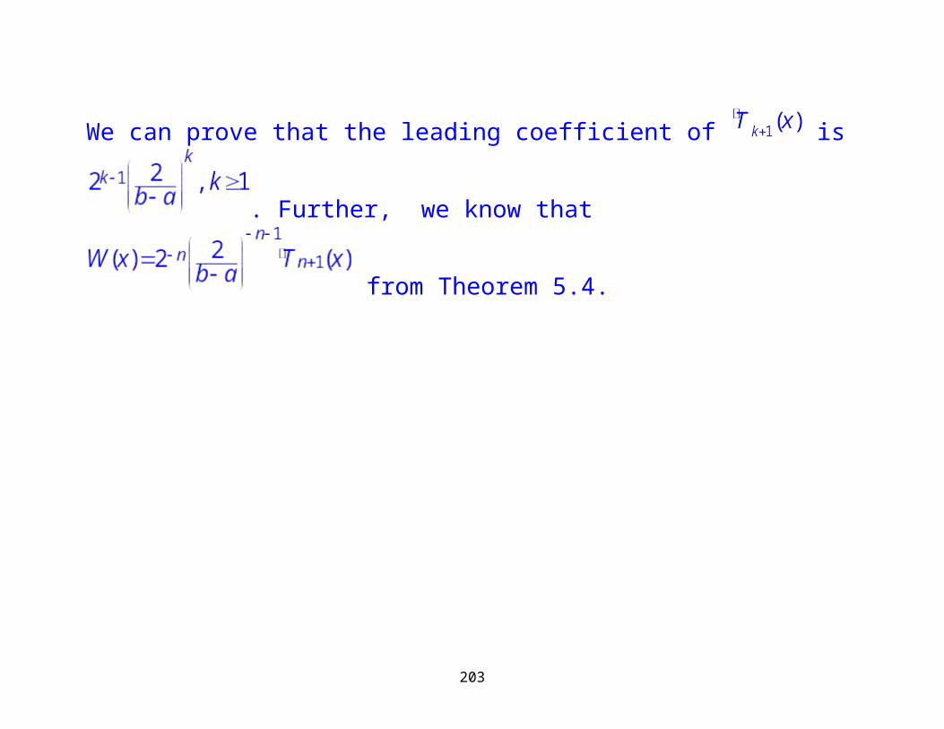
We can prove that the leading coefficient of is .
Further, we know that from Theorem 5.4.
150
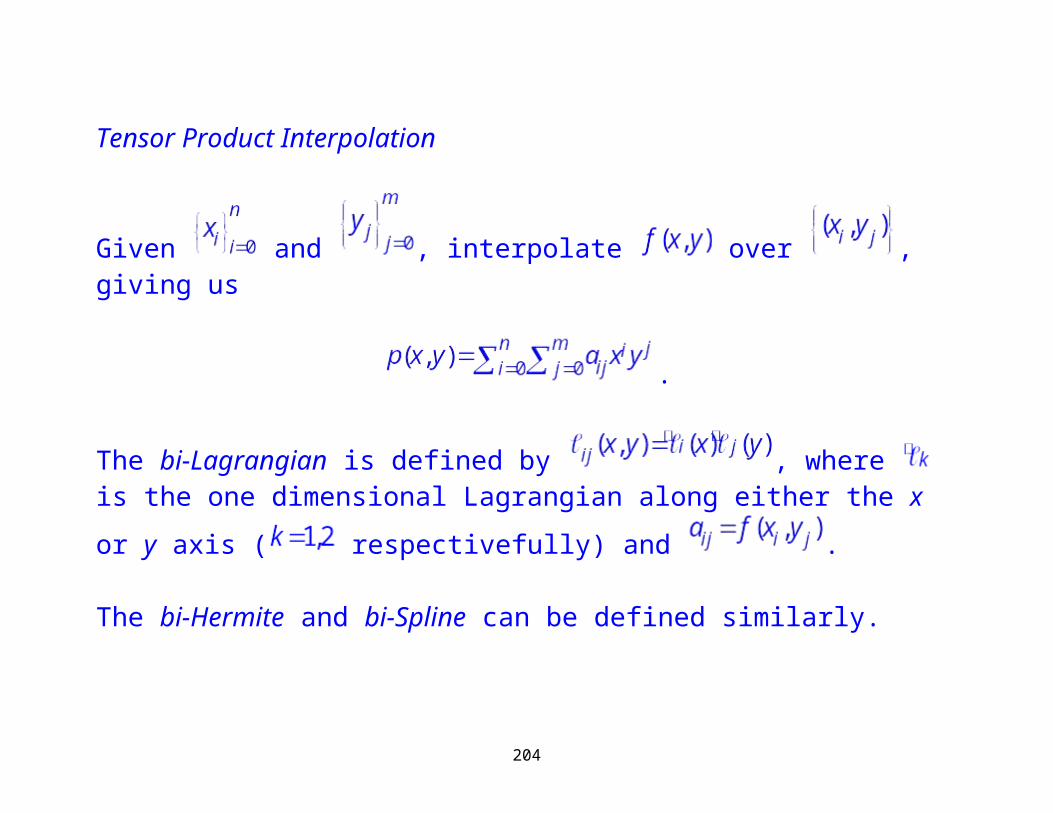
Tensor Product Interpolation
Given and , interpolate over , giving us
.
The bi-Lagrangian is defined by , where is the one dimensional Lagrangian along either the x or y axis ( respectivefully) and
.
The bi-Hermite and bi-Spline can be defined similarly.
151
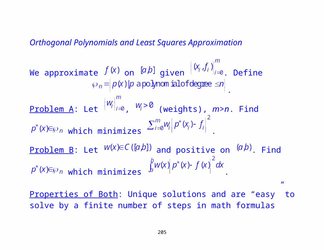
Orthogonal Polynomials and Least Squares Approximation
We approximate on given . Define
.
Problem A: Let , (weights), m>n. Find which minimizes
. Problem B: Let and positive on . Find which
minimizes .
152
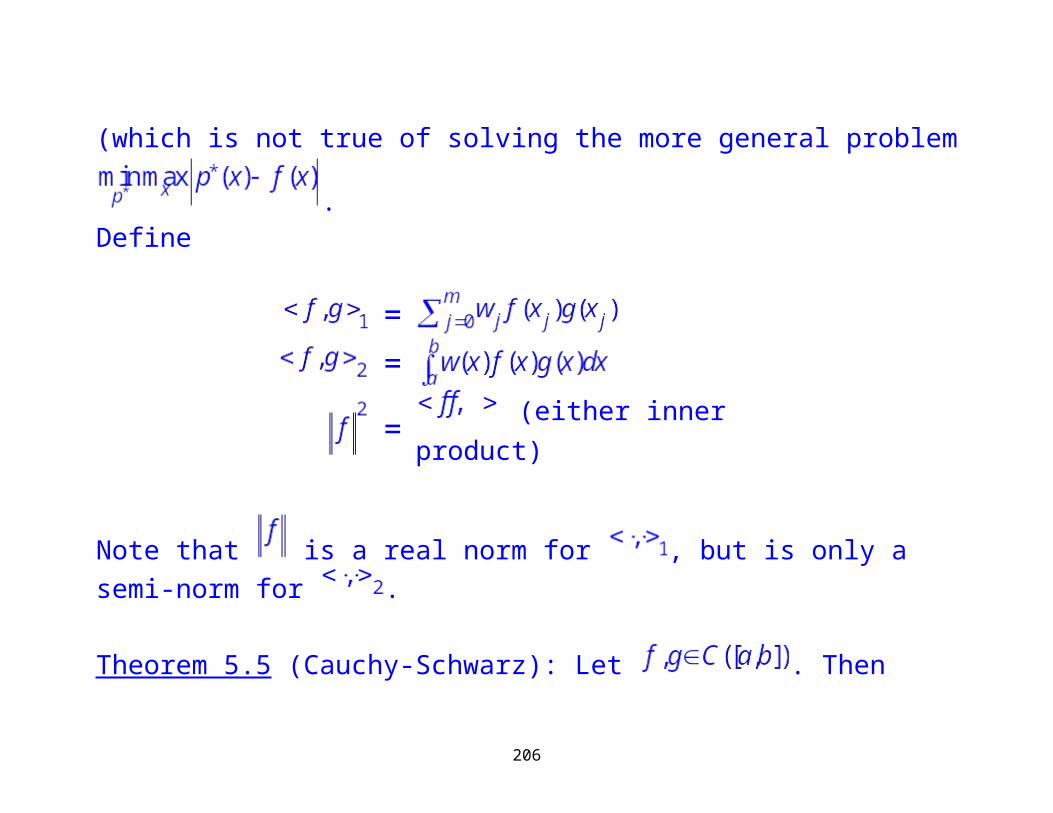
Properties of Both: Unique solutions and are “easy” to solve by a finite number of steps in math formulas (which is not true of solving the more general problem
.Define
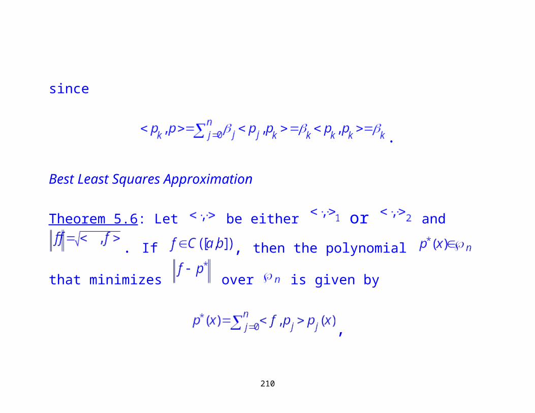
==
= (either inner product)
Note that is a real norm for , but is only a semi-norm for .
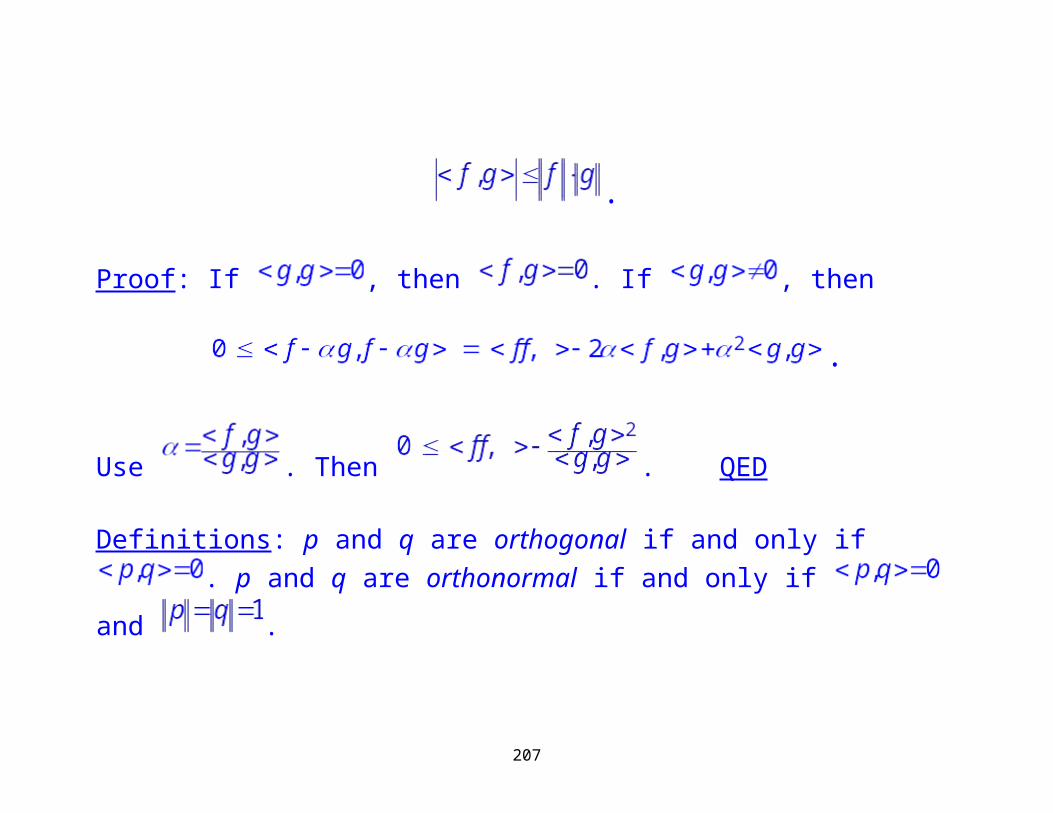
Theorem 5.5 (Cauchy-Schwarz): Let . Then
153
.
Proof: If , then . If , then
.
Use . Then . QED
Definitions: p and q are orthogonal if and only if . p and q are
orthonormal if and only if and .
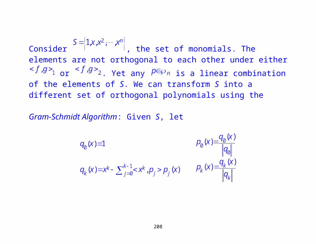
Consider , the set of monomials. The elements are not
orthogonal to each other under either or . Yet any is a
154
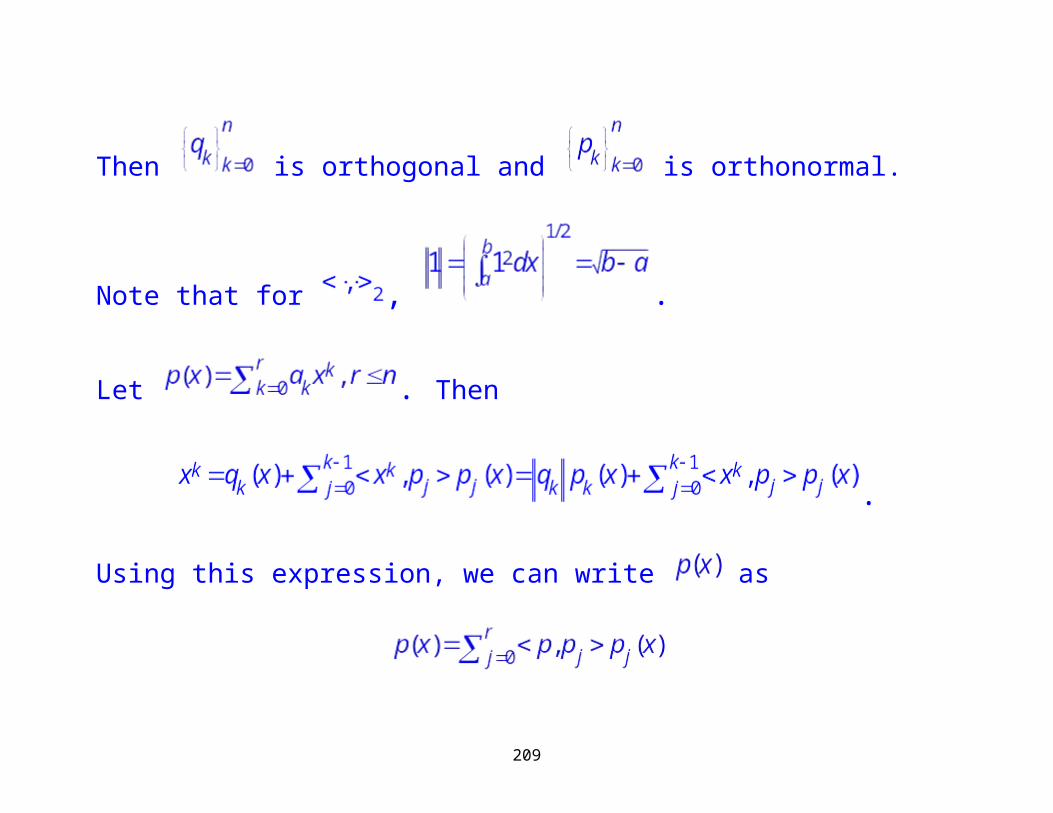
linear combination of the elements of S. We can transform S into a different set of orthogonal polynomials using the
Gram-Schmidt Algorithm: Given S, let
Then is orthogonal and is orthonormal.
Note that for , .
155
Let . Then
.
Using this expression, we can write as
since
.
Best Least Squares Approximation
156
Theorem 5.6: Let be either or and . If
, then the polynomial that minimizes over is given by
,
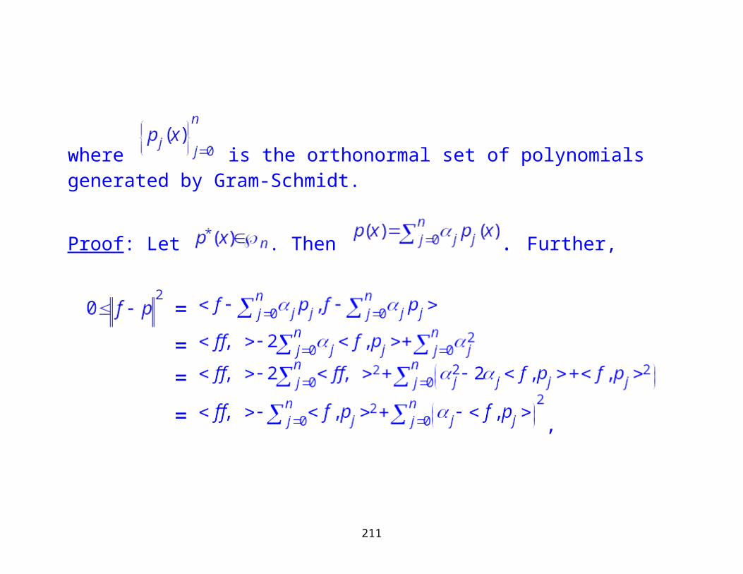
where is the orthonormal set of polynomials generated by Gram-Schmidt.
Proof: Let . Then . Further,
=
157
==
= ,
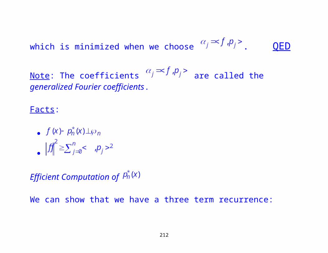
which is minimized when we choose . QED
Note: The coefficients are called the generalized Fourier coefficients.
Facts:
158
Efficient Computation of
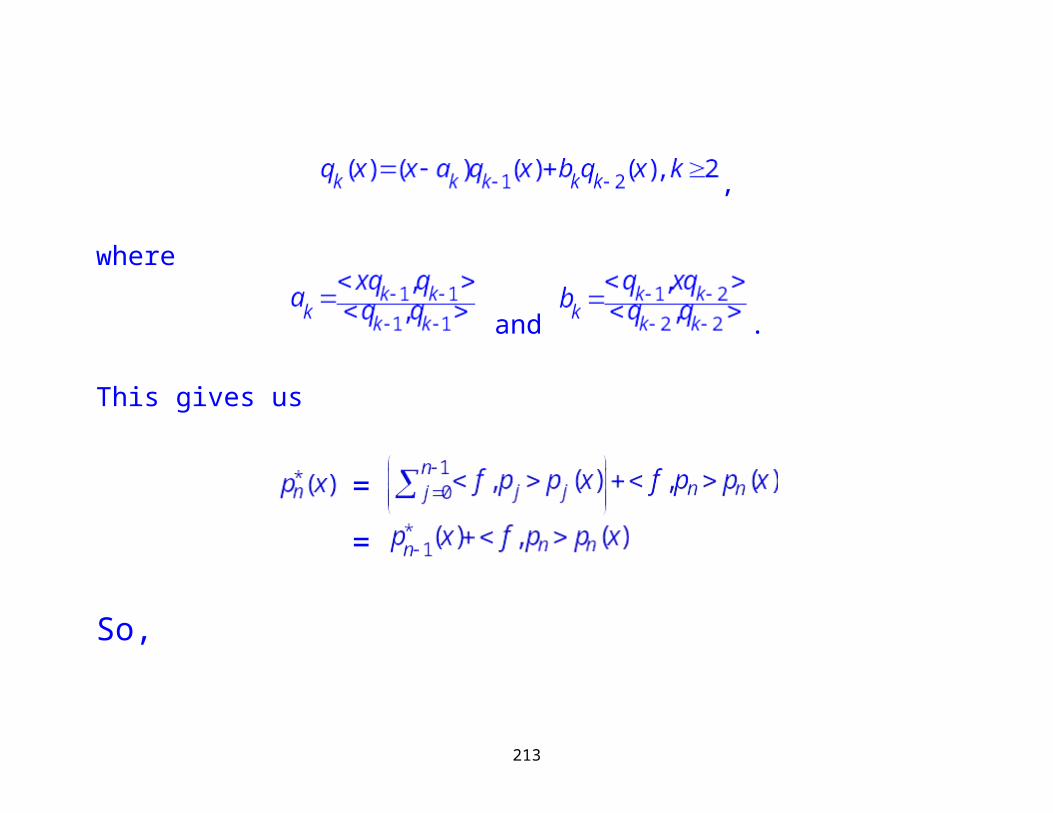
We can show that we have a three term recurrence:
,
where
and .
This gives us
=
=
159
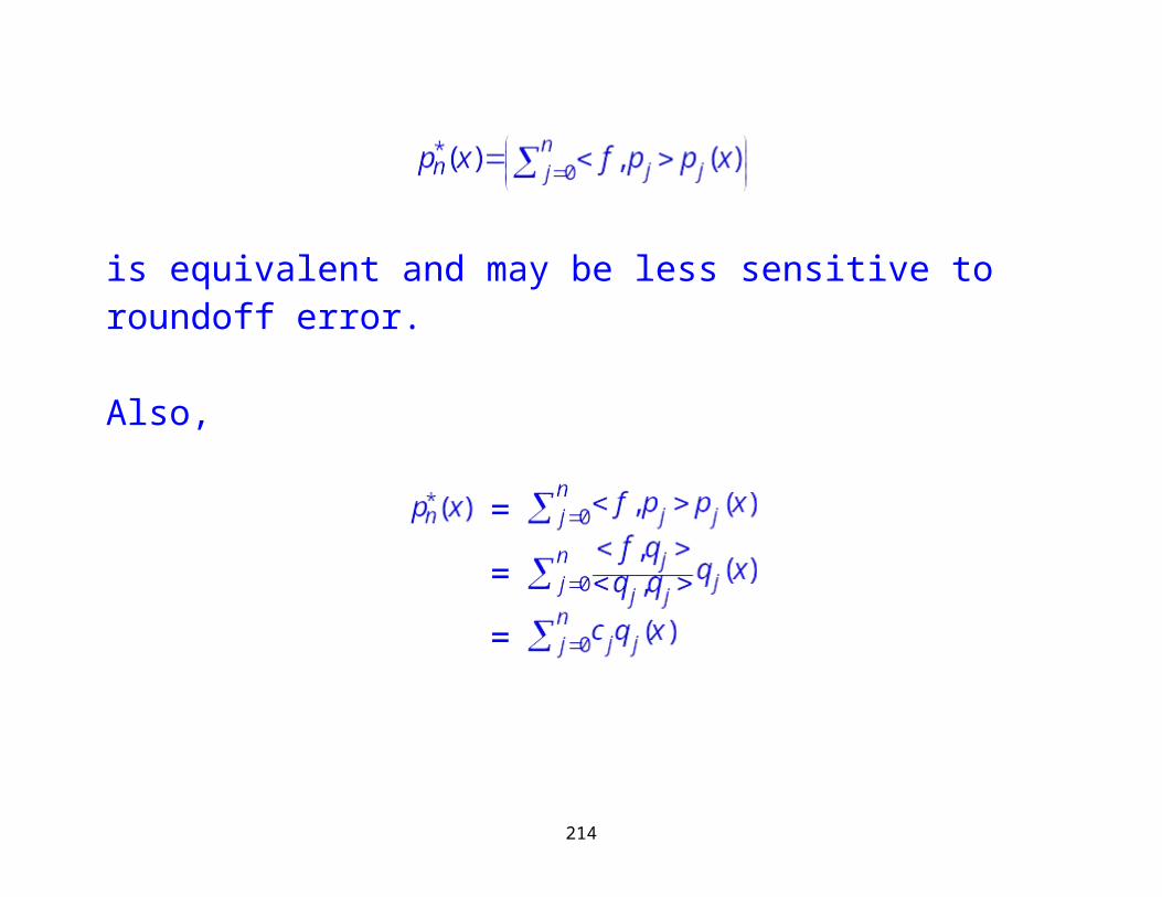
So,
is equivalent and may be less sensitive to roundoff error.
Also,
=
=
=
160
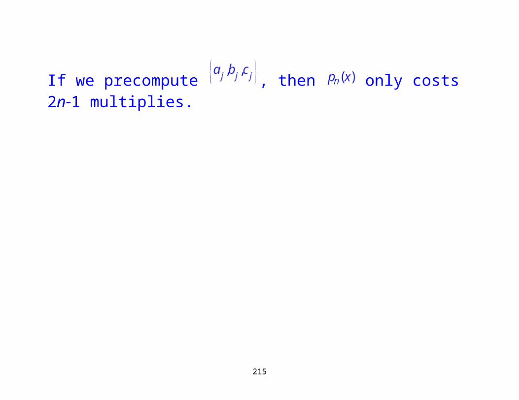
If we precompute , then only costs 2n1 multiplies.
161
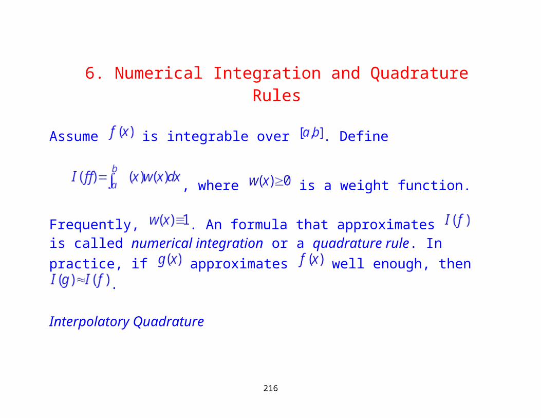
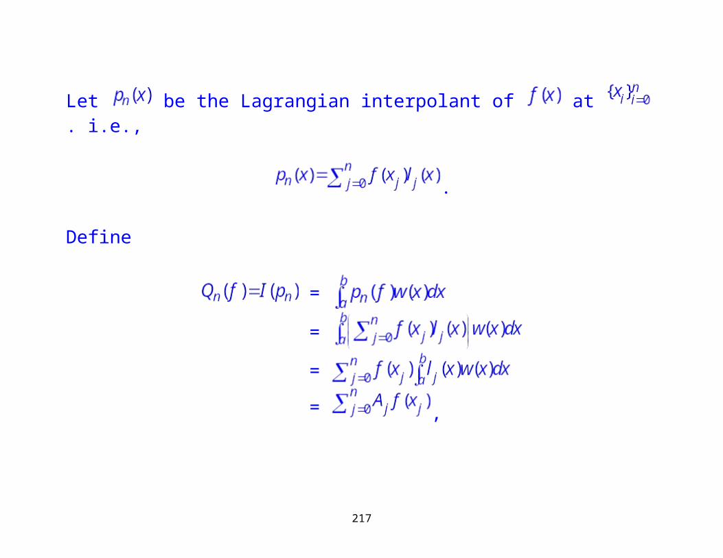
6. Numerical Integration and Quadrature Rules
Assume is integrable over . Define
, where is a weight function.
Frequently, . An formula that approximates is called numerical integration or a quadrature rule. In practice, if approximates well enough, then .
Interpolatory Quadrature
Let be the Lagrangian interpolant of at . i.e.,
.
162
Define
=
=
=
= ,
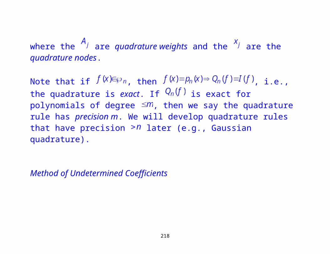
where the are quadrature weights and the are the quadrature nodes.
Note that if , then , i.e., the quadrature is exact. If is exact for polynomials of degree , then we say the quadrature rule has precision m. We will develop quadrature rules that have precision later (e.g., Gaussian quadrature).
163
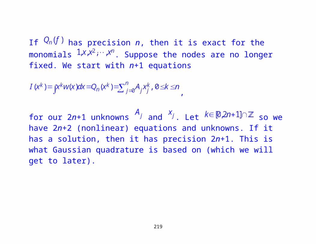
Method of Undetermined Coefficients
If has precision n, then it is exact for the monomials . Suppose the nodes are no longer fixed. We start with n+1 equations
,
for our 2n+1 unknowns and . Let so we have 2n+2 (nonlinear) equations and unknowns. If it has a solution, then it has precision 2n+1. This is what Gaussian quadrature is based on (which we will get to later).
The Trapezoidal and Simpson’s Rules are trivial examples.
Trapezoidal Rule
164
Let . This is derived by direct integration rule. Take
and . Then=
=
=
= .
Simpson’s Rule
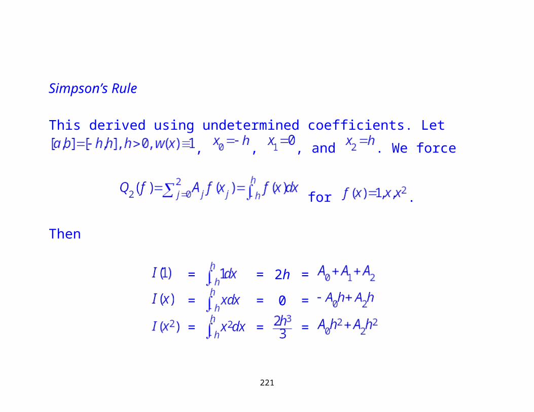
This derived using undetermined coefficients. Let ,
, , and . We force
165
for .
Then
= = 2h =
= = 0 =
= = =
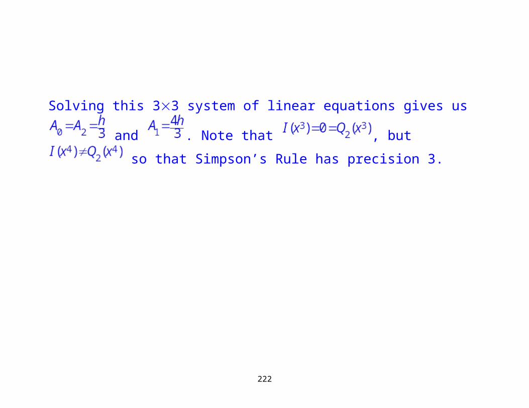
Solving this 33 system of linear equations gives us and .
Note that , but so that Simpson’s Rule has precision 3.
166
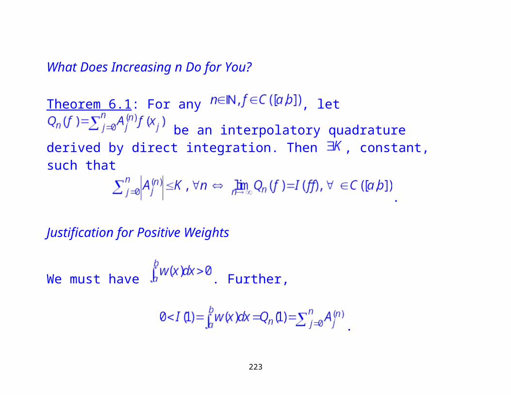
What Does Increasing n Do for You?
Theorem 6.1: For any , let be an interpolatory quadrature derived by direct integration. Then , constant, such that
.
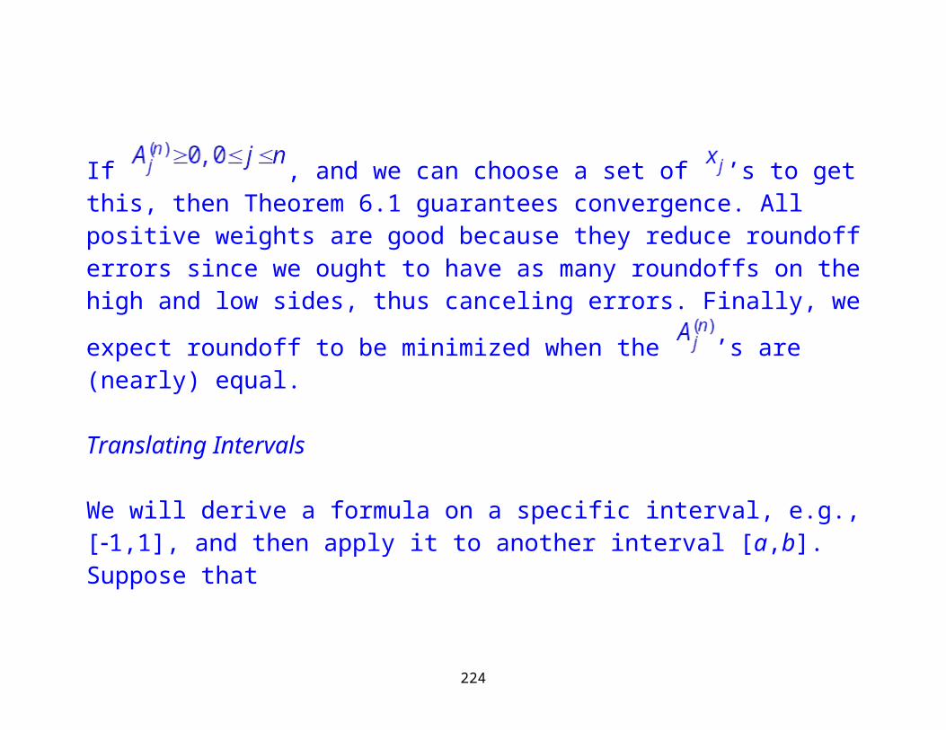
Justification for Positive Weights
We must have . Further,
.
167
If , and we can choose a set of ’s to get this, then Theorem 6.1 guarantees convergence. All positive weights are good because they reduce roundoff errors since we ought to have as many roundoffs on the high and low sides, thus canceling errors. Finally, we expect roundoff to be minimized when
the ’s are (nearly) equal.
Translating Intervals
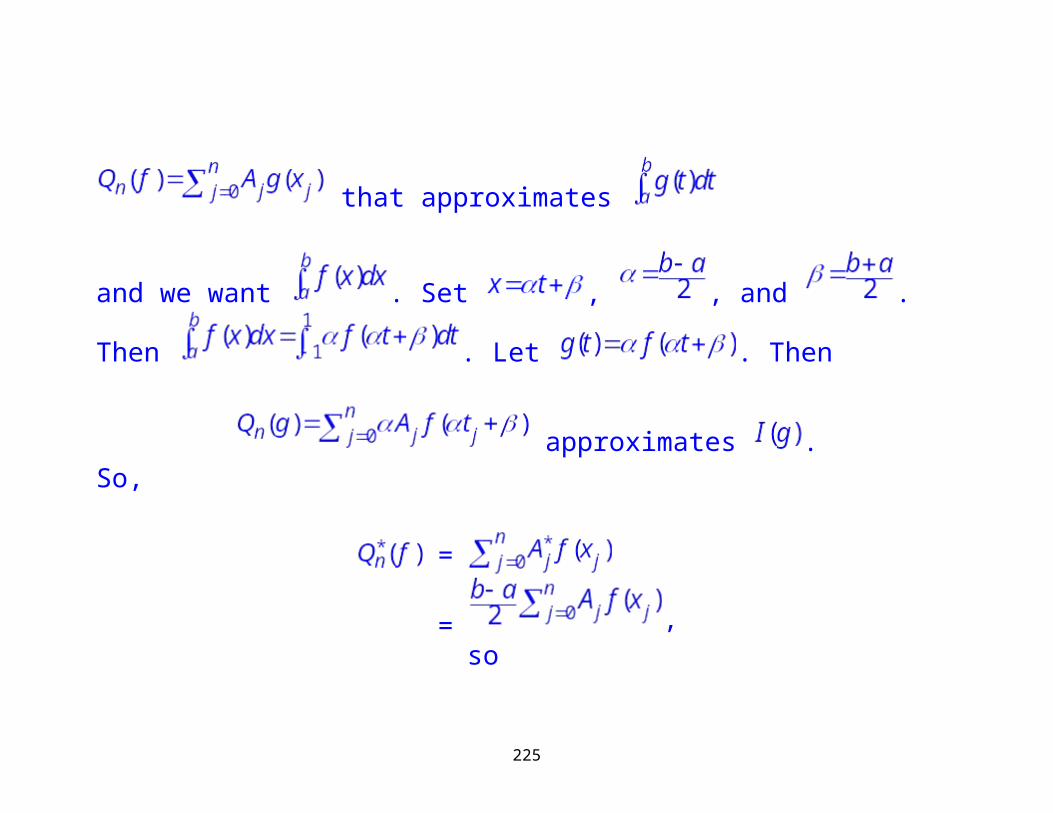
We will derive a formula on a specific interval, e.g., [1,1], and then apply it to another interval [a,b]. Suppose that
that approximates
168
and we want . Set , , and . Then
. Let . Then
approximates .So,
=
= , so
= .
Newton-Coates Formulas
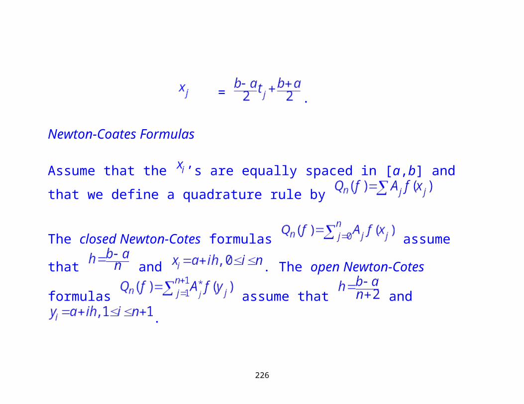
169
Assume that the ’s are equally spaced in [a,b] and that we define a quadrature
rule by
The closed Newton-Cotes formulas assume that
and . The open Newton-Cotes formulas
assume that and .
170
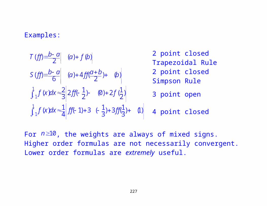
Examples:
2 point closed Trapezoidal Rule
2 point closed Simpson Rule
3 point open
4 point closed
For , the weights are always of mixed signs. Higher order formulas are not necessarily convergent. Lower order formulas are extremely useful.
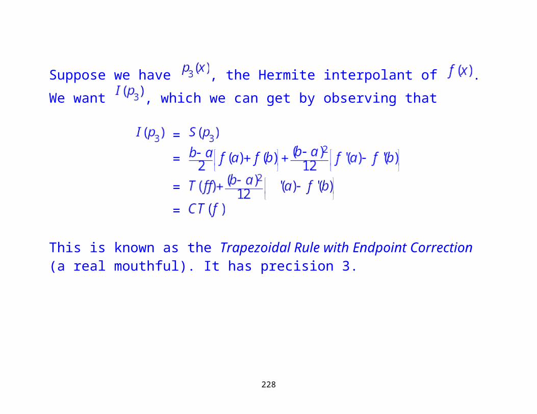
Suppose we have , the Hermite interpolant of . We want , which we can get by observing that
171
=
=
=
=
This is known as the Trapezoidal Rule with Endpoint Correction (a real mouthful). It has precision 3.
172
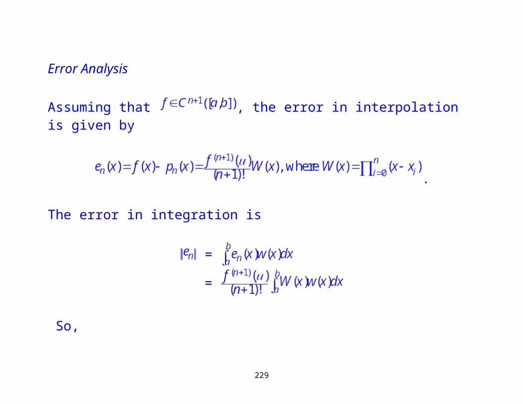
Error Analysis
Assuming that , the error in interpolation is given by
.
The error in integration is
=
=
So,
.
173
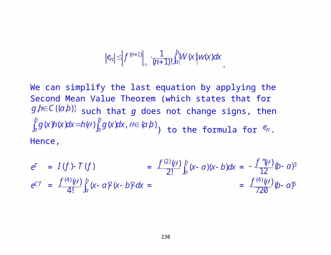
We can simplify the last equation by applying the Second Mean Value Theorem (which states that for such that g does not change signs, then
) to the formula for . Hence,
= = =
= = =
=
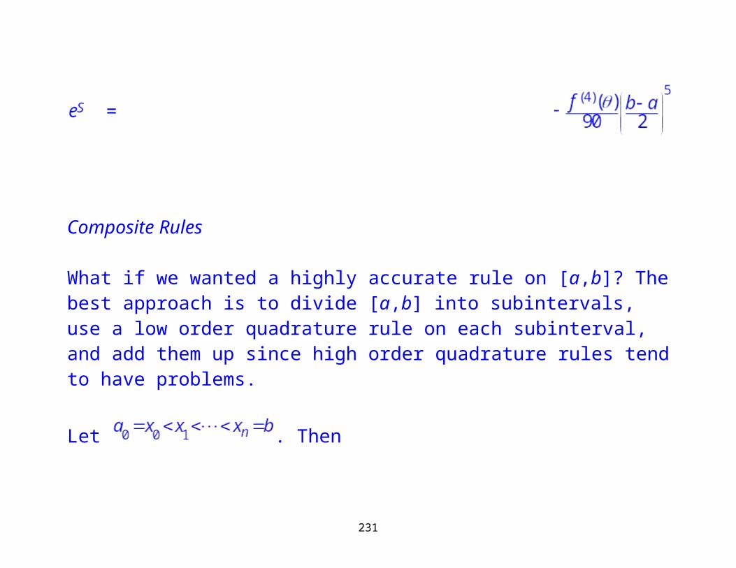
Composite Rules
174
What if we wanted a highly accurate rule on [a,b]? The best approach is to divide [a,b] into subintervals, use a low order quadrature rule on each subinterval, and add them up since high order quadrature rules tend to have problems.
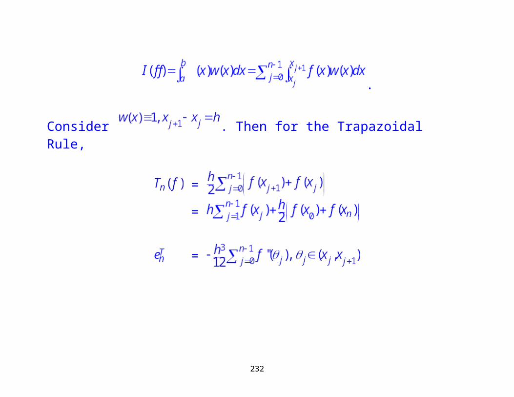
Let . Then
.
Consider . Then for the Trapazoidal Rule,
=
=
175
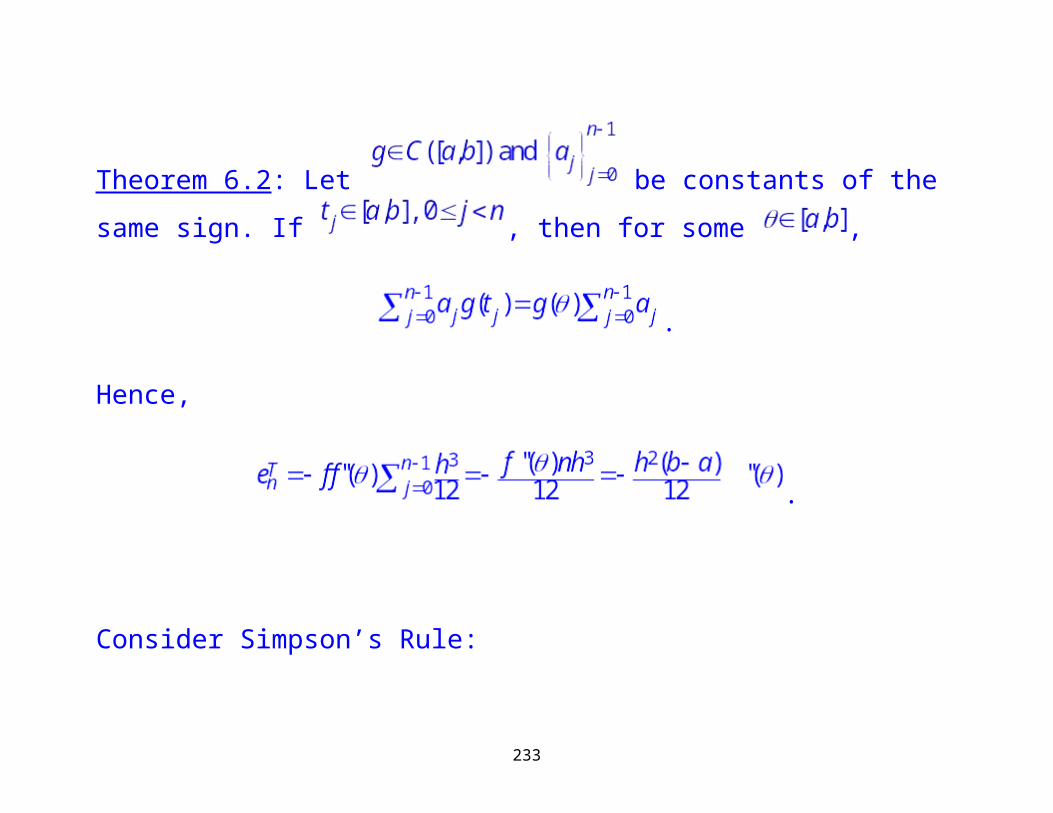
=
Theorem 6.2: Let be constants of the same sign. If
, then for some ,
.
Hence,
.
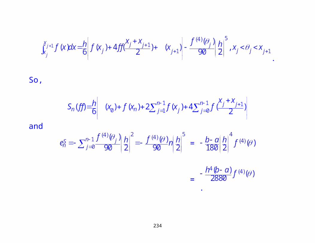
Consider Simpson’s Rule:
176
.
So,
and
=
=.
177
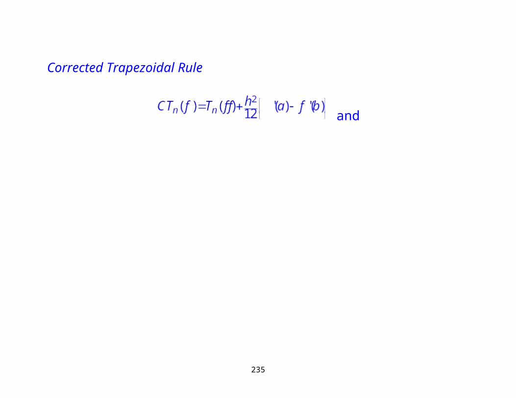
Corrected Trapezoidal Rule
and
178
The number of function evaluations and order of error over n points is
Method Evaluations OrderFunction Derivative
N2N+1
N 2
We can show that
.
If the function evaluation cost is quite high, becomes quite attractive computationally, particularly if the endpoint derivatives are known or quite easy
179
to compute. While and are both , there is a noticeable difference in the constants, which needs to be considered in choosing n.
180
Adaptive Quadrature
Suppose we want to within an error tolerance of and an automatic procedure to accomplish this feat. Consider .
Motivation: Suppose is badly behaved only over , where is a small part of . Then over will be accurate for small n’s, but over may be a very poor approximation to . Doubling n will not necessarily increase accuracy over , where it was already acceptable, and we still not get an acceptable approximation over
. Instead, we want to subdivide and work hard just there while doing minimal work in … and we do not want to know where is in advance!
181
Adaptive quadrature packages accept , f, and and return EST, which supposedly satisfies
.
An error sensing mechanism is used on intermediate steps to control the overall quadrature error. For instance, if and , then
and ,
where . The critical (and sometimes erroneous) assumption is that constant over . This is true when is small in
comparison to how rapidly varies in .
182
Set
.
Then
,
which mean that is 16 times more accurate than when is well behaved on . So,
.
183
We know to compute both and over . Many applications require that EST be very accurate, rather than inexpensive to compute. Hence, we can use a conservative error estimator of the form,
.
Algorithm apparent: Compute and over .
1. If the error is acceptable, then add the estimate of into EST.2. Otherwise, divide into two equal sized intervals and try again in both
intervals. The expected error on both intervals is reduced by a factor of 32.The real estimator must depend on the size of , however. A good choice is
.
184
Theorem 6.3: This estimator will eventually produce a interval that is acceptable.
Proof: Every time we half the interval , the quadrature error decreases by a factor of 32. Set
.If
,then
.
Taking . QED
Theorem 6.4: The cost is only two extra function evaluations at each step.
185
Folk Theorem 6.5: Given any adaptive quadrature algorithm, there exists an infinite number of ’s that will fool the Algorithm Apparent into failing. (Better algorithms work for the usual ’s.)
Proof: Let be 5 equally spaced points used in computing
and . Test
.
If true, then use as an estimate to . If false, then retreat to , where , equally
spaced. Now only evaluations at are necessary if we saved our
previous function evaluations. We test . If the test
186
succeeds, then we pass on to interval , otherwise we work on a new level 3. This process is not guaranteed to succeed. Hence, we need to add an extra condition that
always.
If this fails, then we cannot produce EST. QED
Richardson Extrapolation
This method combines two or more estimates of something to get a better estimate. Suppose
,
where is computable for any . Further, we assume that
187
.
Finally, we assume that
,
where the ’s are independent of h and . Take
with the most common value. We want to eliminate the term using a combination of by noting that
.
We have two definitions of , so we can equate them to compute first + second definitions, or
188
.
189
Set
=
=
=
Then
.
If , then we can repeat this process to eliminate the term. Define
190
Then
and
Applications of Richardson Extrapolation
Differentiation is a primary application. Assume that .
First, try for small h, . The Taylor expansion about gives us
,
191
where the ’s are independent of h and probably unknown.
Second, try . We can prove that
We can modify the definition of to use Then
Next extrapolatation must be of the form . So,
.
Use this formula whenever
192
Romberg Integration
On , approximate . Define
,
where . This choice of eliminates half of the
function evaluations when computing . The error only contains even powers of h. Hence,
193
or .Continue extrapolation as long as
.
Roundoff error is the typical culprit for stopping Richardson extrapolation.
194
7. Automatic Differentiation (AD)
This is a technique to numerically evaluate the derivative of a function using a computer program. There have been two standard techniques in the past:
Symbolic differentiation Numerical differentiation
Symbolic differentiation is slow, frequently produces many pages of expressions instead of a compact one, and has great difficulty converting a computer program. Numerical differentiation involves finite differences, which are subject to roundoff errors in the discretization and cancellation effects. Higher order derivatives exasperate the difficulties of both techniques.
“Automatic differentiation solves all of the mentioned problems.” Wikipedia
Throughout this section, we follow Wikipedia’s AD description and use its figures. The most comprehensive AD book is Griewank’s SIAM 300 pager.
195
The primary tool of AD is the chain rule,
for a function .
There are two ways to traverse the chain rule:
Right to left, known as forward accumulation. Left to right, known as backward accumulation.
196
Assume that any computer program that evaluates a function can be decomposed into a sequence of simpler, or elementary partial differivatives, each of which is differentiated using a trivial table lookup procedure. Each elementary partial derivative is evaluated for a particular argument using the chain rule to provide derivative information about F (e.g., gradients, tangents, Jacobian matrix, etc.) that is exact numerically to some level of accuracy. Problems with symbolic mathematics are avoided by only using it for a set of very basic expressions, not complex ones.
197
Forward accumulation
First compute then in .
Example: Find the derivative of . We have to seed the expression to distinguish between the derivative for and .
Original code statements Added AD statements
(seed)
(seed)
198
Forward accumulation traverses the figure from bottom to top to accumulate the result.
199
In order to compute the gradient of f, we have to evaluate both and , which corresponds to using seeds and , respectively.
The computational complexity of forward accumulation is proportional to the complexity of the original code.
Reverse accumulation
First compute then in .
Example: As before. We can produce a graph of the steps needed. Unlike, forward accumulation, we only need one seed to walk through the graph (from top to bottom this time) to calculate the gradient in half the work of forward accumulation.
200
Superiority condition of forward versus reverse accumulation
Forward accumulation is superior to reverse accumulation for functions . Reverse accumulation is superior to forward accumulation
for functions .
201
Jacobean computation
The Jacobean J of is a matrix. We can compute the Jacobian using either
n sweeps of forward accumulation, where each sweep produces a column of J.
m sweeps of backward accumulation, where each sweep produces a row of J.
Computing the Jacobian with a minimum number of arithmetic operations is known as optimal Jacobian accumulation and has been proven to be a NP-complete hard problem.
202
Dual numbers
We define a new arithmetic in which every is replaced by , where and is nothing but a symbol such that . For regular arithmetic, we
can show that
,
,
and similarly for subtractraction and division. Polynomials can be calculated using dual numbers:
=
=
= ,
203
where represents the derivative of P with respect to its first argument and is an arbitrarily chosen seed.
The dual number based arithmetic we use consists of ordered pairs with ordinary arithmetic on the first element and first order differential arithmetic on the second element. In general for a function f, we have
,
where represent the derivative of f with respect to the first and second arguments, respectively. Some common expressions are the following:
and
204
and
and
and
and
The derivative of at some point in some direction is given by
205
using the just defined arithmetic. We can generalize this method to higher order derivatives, but the rules become quite complicated. Truncated Taylor series arithmetic is typically used instead since the Taylor summands in a series are known coefficients and derivatives of the function in question.
Implementations
Google “automatic differentiation” and just search through the interesting sites.
Oldies, but goodies:
ADIFOR (Fortran 77) ADIC (C, C++) OpenAD (Fortran 77/95, C, C++) MAD (Matlab) – not recommended!
Typically, the transformation process is similar to the following:
206
8. Numerical Differential (Finite Differences)
Assume . Then
for all . This suggests a finite difference approach to estimating . Let
.
For simplicity assume that
207
,
which is known as a uniform mesh. We will use Taylor expansions about one of more points liberally, e.g.,
There are 3 common first differences of note:
Forward
Backward
208
Central
While the forward and backward differences are 1st order with mesh spacing h, they are second order for mesh spacing h/2 for midpoints !
To get an approximation to the 2nd derivative, we add two Taylor expansions about the points to get
, which is .
These formulae are frequently reduced to stencils involving only 2-3 adjacent points in the mesh:
209
.
There are many more formulae with specific properties that can be derived by matching terms in specific Taylor expansions.
Example (upwind difference): Find a one sided, 2nd order finite difference for , i.e.,
.
Expand about the points of interest to see that
c: =
b: =
210
a: =
211
So,
=
=
We are left solving
or .
Hence,
212
The stencil is . Note that the trailing 0’s are sometimes left off if the meaning is completely clear. In practice, with a stencil based code, the 0’s usually are left off since the ith location in the stencil has to be specified.
We can apply finite differences to an elliptic differential equation with boundary values, which is also known as an elliptic boundary-value problem (BVP). This one is also known as Laplace’s equation in one dimension (1D):
On a uniform mesh we get the following system of linear equations:
213
,
which is nonsymmetric. We can eliminate the first and last rows and columns (since we know the boundary values of u) to get an symmetric, positive definite system of linear equations instead. Any of the methods we used earlier for solving systems of linear equations (direct or iterative) work well to solve this problem.
214
Variable coefficients can be handled by taking the correct Taylor expansions and combining them. Consider the differential equation
.
Suitable Taylor expansions lead to a finite difference scheme of
,
which is .
Question: What happens when is unavailable to evaluate? Then has to be interpolated to or better. This leads to another error term.
215
Error analysis of finite difference schemes leads to considering what is known as the Lax equivalence theorem, which can be summarized by
Consistency + Stability = Convergence.
Consistency determines the order of accuracy of a difference scheme plus the truncation error.
Stability determines the frequency distribution of the error (usually by investigating eigenvalue type analysis).
Absoulte stability is based on considering . We want
and prefer that .
Conditional stability is simlar, but there is at least one condition to guarantee stability.
216
Time and Space finite differences
Consider an initial value problem (IVP)
.
If , then there are very efficient special methods, which are in the textbook, but not here. Consider some typical explicit cases:
Forward Euler or
Leapfrog
Multistep
217
The general formula for a k-step scheme is
with (normalization) and either (explicit) or (implicit).
Example: Adams-Bashford family
1st order Forward Euler
2nd order
3rd order
218
The first few steps use lower order methods, which can cause problems and spurious errors in later time steps.
Multi-stage methods use a weighted sum of corrections within one time step. So,
219

The Ck are determined by matching terms in a Taylor expansion. Typically,
(Forward Euler)
220
Runge-Kutta methods are popular and usually either Total Variation Diminshing (TVD) or … Bounded (TVB), which do not allow any spurious oscillations to appear in the numerical solution and ruin all further calculations.
RK2 / 2 level storage scheme:
Set .
Compute
Update
Note that is the modified Euler method and is Heun’s method.
221
Classic RK4 / 4 levels of storage:
Compute
and
Update
Note that there is a trick that reduces this scheme to only 3 levels of storage.
222
Implicit Time Stepping:
Consider the IVP . The family of methods is defined by
.
Note that =0 is Forward Euler (explicit), =1 is Backward Euler (implicit), and =1/2 is Crank-Nicolson (implicit). For implicit methods, some sort of direct solver is implied (or an iterative methods approximation).
Consistency:
As , the right hand side goes to zero, so we recover the IVP.
223
Stability: We study So, . Looking at the error at the nth step and doing some algebraic manipulations, we get
.
We have absolute stability if .
Conditional stability and requires that .
Unconditional stability whenever .
For Forward Euler, we must have , which is a very serious constraint as . Implicit methods are more expensive per step, but can use much, much
224
bigger time steps.9. Monte Carlo Methods
Monte Carlo (MC) methods use repeated random sampling to solve computational problems when there is no affordable deterministic algorithm. Most often used in
Physics Chemistry Finance and risk analysis Engineering
MC is typically used in high dimensional problems where a lower dimensional approximation is inaccurate.
Example: n year mortgages paid once a month. The risk analysis is in 12n dimensions. For a 30 year mortgage we have a 360 dimensional problem. Integration (quadrature rules) above 8 dimensions is impractical.
225
Main drawback is the addition of statistical errors to the systematic errors. A balance between the two error types has to be made intelligently, which is not always easy nor obvious.
Short history: MC methods have been used since 1777 when the Compte de Buffon and Laplace each solved problems. In the 1930’s Enrico Fermi used MC to estimate what lab experiments would show for neutron transport in fissile materials. Metropolis and Ulam first called the method MC in the 1940’s. In 1950’s MC was expanded to use an probability distribution, not just Gaussian. In the 1960’s and 1970’s, quantum MC and variational MC methods were developed.
MC Simulations: The problem being solved is stochastic and the MC method mimics the stochastic properties well. Example: neutron transport an decay in a nuclear reactor.
226
MC Calculations: The problem is not stochastic, but is solved using a stochastic MC method. Example: high dimension integration.Quick review of probability
Event B is a set of possible outcomes that has probability . The set of all events is denoted by and particular outcomes are . Hence, .
Suppose . Then represents events in both B and C. Similarly, represents events that are in B or C.
Some axioms of probability are1.2. 3. 4.
227
The conditional probability that a C outcome is also a B outcome is given by Bayes formula,
.Frequently, we already know both and and use Bayes formula to calculate .
Events B and C are independent if .
If is either finite or countable, we call discrete. In this case we can specify all probabilities of possible outcomes as
and an event B has probability
228
.
A discrete random variable is a number that depends on the random outcome . As an example, in coin tossing, could represent how many
heads or tails came up. For , define the expected value by
.
The probability distribution of a continuous random variable is described using a probability density function (PDF) . If and , then
and .
The variance in 1D is given by
229
.
The notation is identical for discrete and continuous random variables.For 2 or higher dimensions, there is a symmetric variance/covariance matrix given by
,
where the matrix elements are given by
.
The covariance matrix is positive semidefinite.
230
Common random variables
The standard uniform random variable U has a probability density of
We can create a random variable in [a,b] by . The PDF for Y is
The exponential random variable T with rate constant has a PDF
231
The standard normal is denoted by Z and has a PDF
.
The general normal with mean and variance is given by and has PDF
.
We write in this case. A standard distribution has .
If an n component random variable X is a multivariate normal with mean and covariance C, then it has a probability density
232
.
Multivariate normal possess a linear transformation property: suppose L is an matrix with rank m, so and onto. If are
multivariate normal, then the covariance matrix for Y is
assuming that .
Finally, there are two probability laws/theorems that are crucial to believing that MC is relevant to any problem:
1. Law of large numbers2. Central limit theorem
Law of large numbers: Suppose and . The approximation of A is
233
as .
All estimators satisfying the law of large numbers are denoted consistent.
Central limit theorem: If , then .
Hence, recalling that A is not random, that
.
The law of large numbers makes the estimator unbiased. The central limit theorem follows from the independence of the . When n is large enough, is approximately normal, independent of the distribution of X as long as
.
234
Random number generators
Beware simple random number generators. For example, never, ever use the UNIX/Linux function rand. It repeats much too quickly. The function random repeats less frequently, but is not useful for parallel computing. Matlab has a very good random number generator that is operating system independent.
Look for digital based codes developed 20 years ago by Michael Mascagni for good parallel random number generators. These are the state of the art even today.
However, the best ones are analog: they measure the deviations in the electrical line over time and normalize them to the interval . Some CPUs do this as a hardware instruction for sampling the deviation. These are the only true random number generators available on computers. The Itanium2 CPU line has this built in. Some other chips have this, too, but finding operating systems that will sample this instruction is hard to find.
235
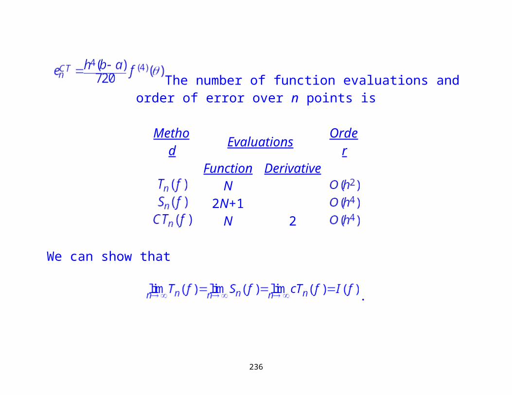
Sampling
A simple sampler produces and independent sample of X each time it is called. The simple sampler turns standard uniforms into samples of some other random variable.
MC codes spend almost all of their time in the sampler. Optimizing the sampler code to reduce its execution time can have a profound effect on the overall run time of the MC computation.
In the discussion below rng() is a good random number generator.
236
Bernoulli coin tossing
A Bernoulli random variable with parameter p is a random variable X with
.
If U is a standard uniform, then . So we can sample X using the code fragment
if ( rng() <= p ) X = 1; else X = 0;
For a random variable with a finite number of values
,
we sample it using the unit interval and dividing it into subintervals of length pk. This works well with Markov chains.
237
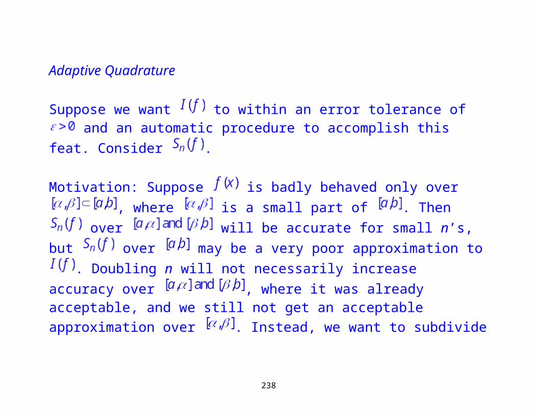
Exponential
If U is a standard uniform, then
is an exponential with rate parameter with units 1/Time. Since 0<U<1, and T>0. We can sample T with the code fragment
T = -(1/lambda)*log(rng());
The PDF of the random variable T is given by for some t>0.
238

Cumulative density function (CDF)
Suppose X is a one component random variable with PDF . Then the CDF
. We know that there is an x such that .
The simple sampler can be coded with
1. Choose U = rng()2. Find X such that
Note that step 2 can be quite difficult and time consuming. Good programming reduces the time.
There is no elementary formula for the cumulative normal . However there is software available to compute it to approximately double precision. The inverse cumulative normal can also be approximated.
239
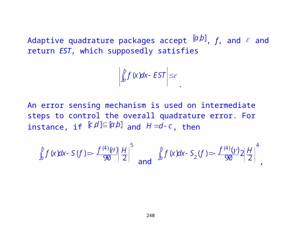
The Box Muller method
We can generate two independent standard normal from two independent standard uniforms using the formulas
We can make N independent standard normal by making N standard uniforms and then using them in pairs to make N/2 pairs of independent standard normal.
240
Multivariate normals
Let be a multivariate normal random variable with mean 0 and covariance matrix C. We sample X using the Cholesky factorization of , where L is lower triangular. Let be a vector of n independent standard normal generated by the Box Muller method (or similarly). Then . If
, then X is multivariate normal and has .
There are many more methods that can be studied, e.g., Rejection.
Testing samplers
All scientific software should be presumed wrong until demonstrated to be correct. Simple 1D samplers are testing using tables and histograms.
241
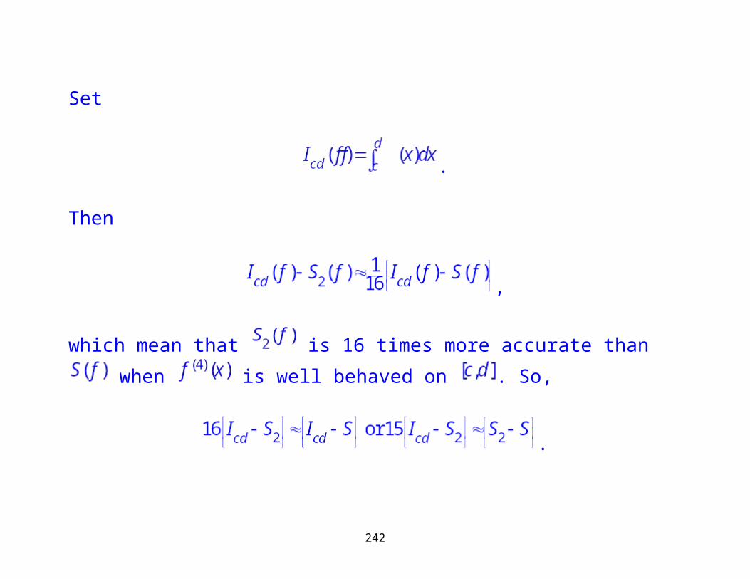
Errors
Estimating the error in a MC calculation is straightforward. Normally a result with an error estimate is given when using a MC method.
Suppose X is a scalar random variable. Approximate by
. The central limit theorem states that is the standard
deviation of and . It can be shown that
, where ,
which we estimate using
then take .
242
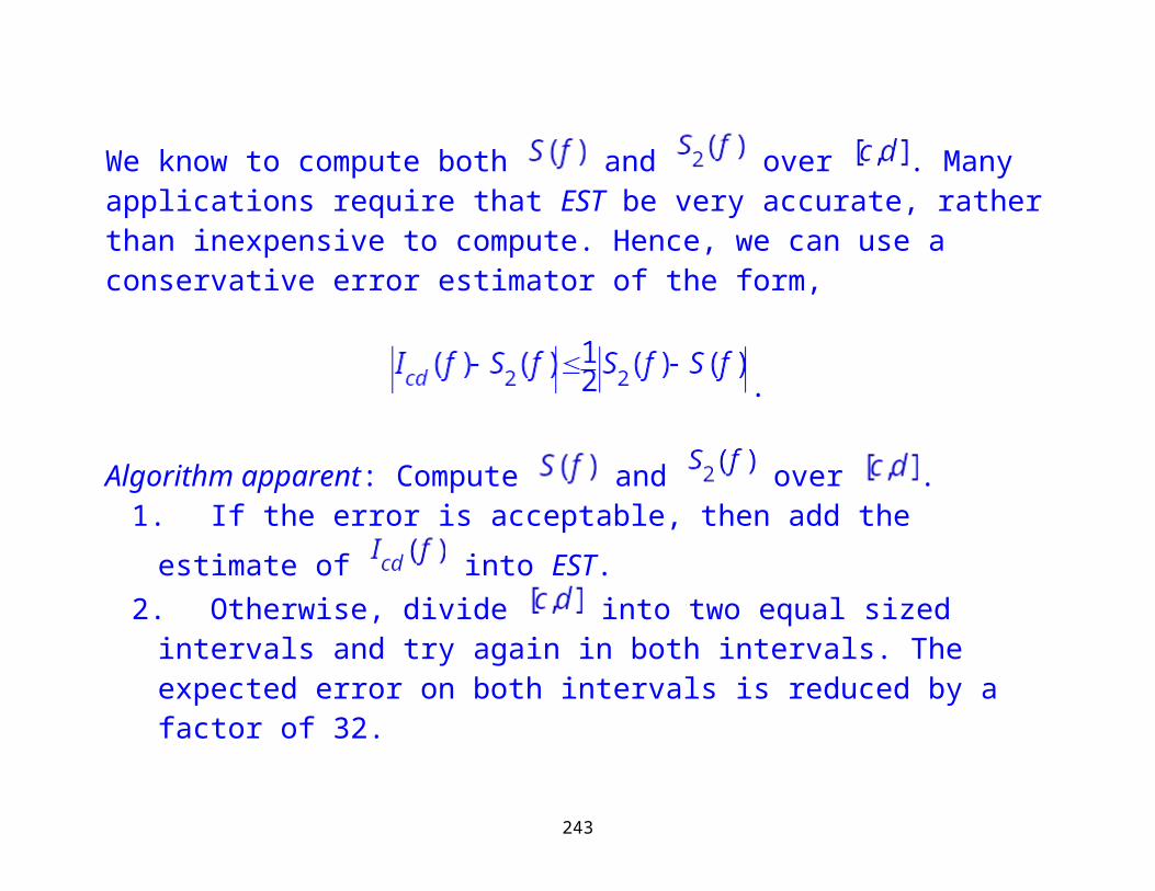
Since Z is of order 1, is of order .
We typically report the MC data as . We can plot circles with a line for the diameter called the (standard deviation) error bar. We can think of k
standard deviation error bars , which are confidence levels. The central limit theorem can be used to show that
and .
It is common in MC to report one standard deviation error bar. To interpret the data correctly, knowledge that the real data is outside of the circle one-third of the time has to be understood.
243
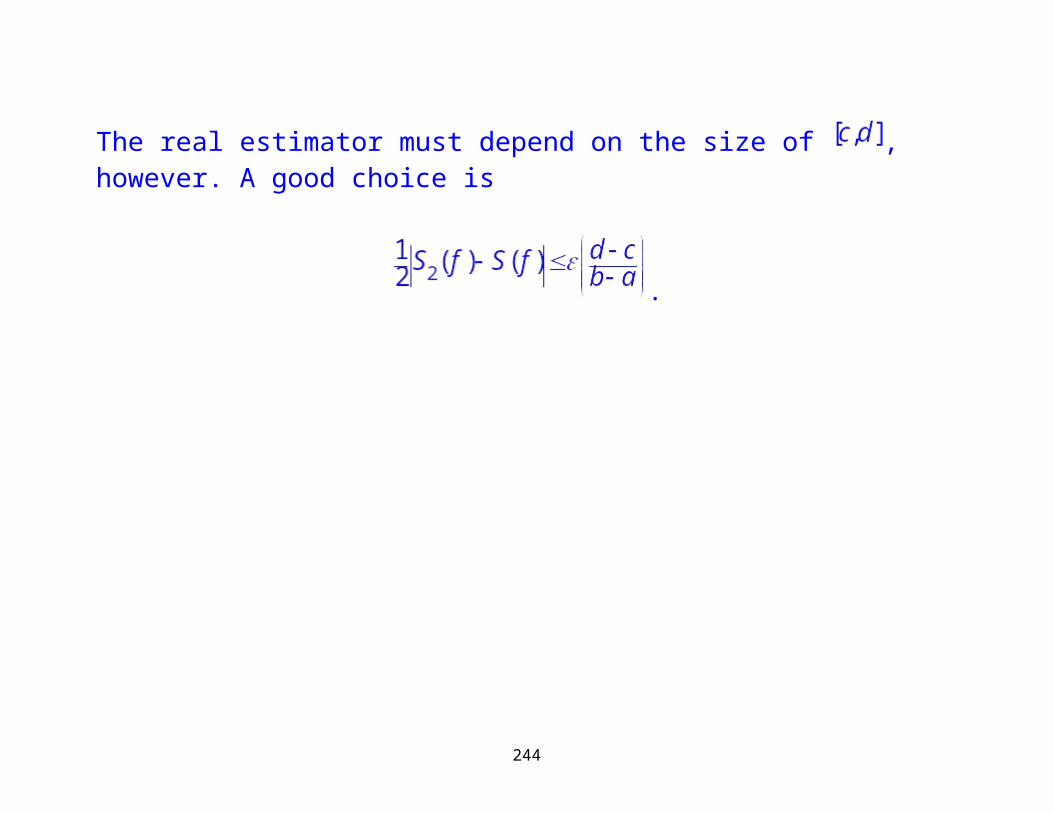
Integration (quadrature)
We want to approximate a d dimensional integral to an accuracy of . Assume we can do this using N quadrature points. Consider Simpson’s rule. For a function , . MC integration can be done so that
independent of d as long as the variance of the integrand is finite.
MC integration
Let V be the domain of integration. Define and for uniform let
and .Then
.
244