EXPLORATIONS IN ECONOMIC HISTORY 28, 274-286 (1991)

Discontinuities in Canadian Economic Growth, 1870-l 985

KRIS INWOOD AND THANASIS STENGOS”

Department of Economics, University of Guelph

INTRODUCTION

Economic historians as diverse as Karl Marx, Lloyd Reynolds, and Walt Rostow view economic development in distinct periods separated by a change in the trend rate or pattern of growth. If the economy simulta- neously experiences cyclical change, however, the change in trend can be difficult to identify. A useful example is presented by the debate about Canada’s early 20th century growth spurt, the “wheat boom.” Was the wheat boom a particularly exuberant upward cycle, or did it mark the beginning of a new and fundamentally different growth process (Hartland, 1955)?

In a macroeconomic context this question is recognized as a problem of correctly decomposing a time series into trend and cyclical movements (Stock and Watson, 1988). Perron (1989) has proposed a technique to determine if exogenous shocks derived from war, technological innova- tion, or other international market changes were sufficiently powerful to alter the underlying trend rate of growth. Use of this technique on Can- ada’s new national income data over the period from 1870 to 1985 leads to the conclusion that the wheat boom and each of the two World Wars created a structural break in the growth process and that no other ex- ogenous shock had a comparable impact.

In the next section we provide a brief synopsis of Canadian growth between 1870 and 1985. In Section III we outline the technique used to determine if particular shocks had the effect of changing the trend rate of growth; technical aspects of the procedure are confined to an appendix.

* We are grateful to the Social Sciences and Humanities Research Council of Canada for financial support in the preparation of this paper. Helpful comments have been received from Lou Cain, Larry Neal, Angela Redish, our colleagues at Guelph, and the anonymous referees of this journal. The authors assume all responsibility for remaining errors and weaknesses.

274

0014-4983/91 $3.00 Copyright 0 1991 by Academic Press, Inc. All rights of reproduction in any form reserved.

CANADIAN ECONOMIC GROWTH 275

12-

1910 1950 1890 1930 1970

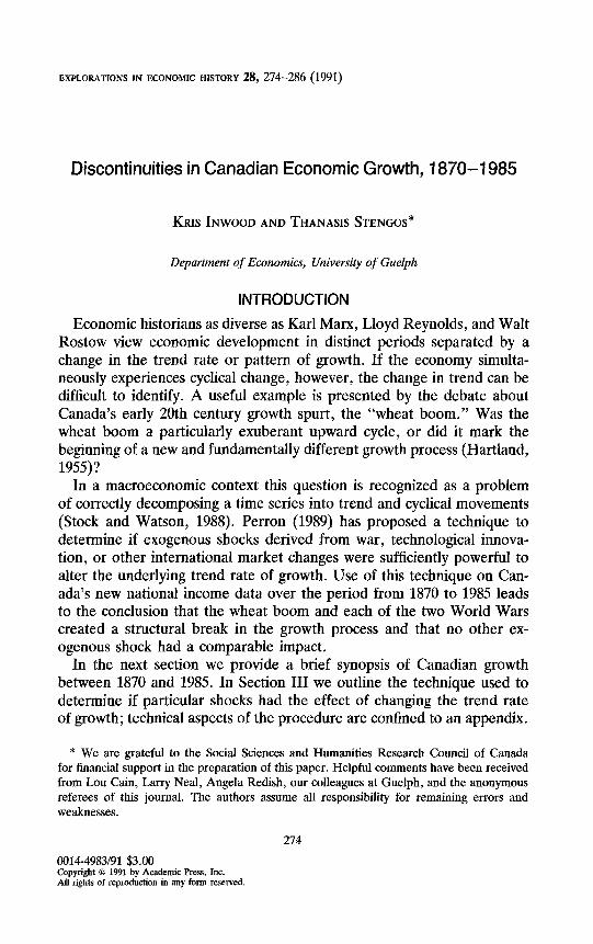
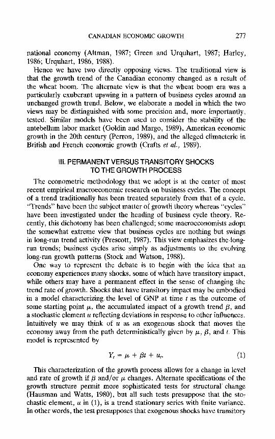
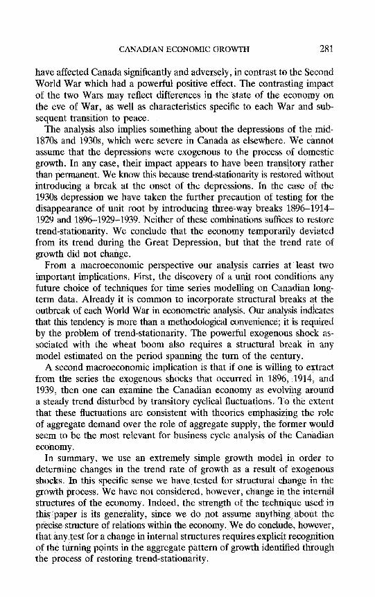
FIG. 1. Log of real GNP with trend lines.

In Section IV we conclude with a brief interpretation of the test results and point to several implications for economic historians of Canada.

It. EXTERNAL SHOCKS AND THE CANADIAN ECONOMY, 1870-f 985

New estimates of Canadian national income from 1870 to 1926 have confirmed that the engine of Canadian growth was impressively strong during the 19th century and then accelerated during the late 1893s in response to an exogenous shift in the Canadian demand for Canadian wheat (Wrquhart, 1986, 1988). This acceleration around the turn of the century has come to be known as the “wheat boom.” Economic growth during the wheat boom decade from 1900 to 1910 was the fastest ever recorded in Canada and investments share of Canadian GNP reached its highest ever level (Fig. 1).

The economy decelerated abruptly in the First World War; per capita income and labor productivity actually contracted during the decade. The government share of GNP temporarily doubled while investment declined from 34% in 1912 to only 12% of GNP in 1918. War-related shipments of foodstuff and materiel loom large in the national accounts as the ex- port/GNP ratio rose dramatically. Although the War’s impact was less dramatic than in Europe, the rise of government spending and other war- related market disturbances had major domestic repercussions (Naylur, 1981). Growth improved after the First World War although not to its prewar level. Investment was less than 20‘% of GNP almost continuously

276 INWOOD AND STENGOS

from 1915 to 1948 and sank to record lows in 1933 and 1943-1944 (Sa- farian, 1970).

During World War Two public spending again grew as the government share of the economy more than tripled to 42% in 1944. In the immediate post-war period government activity diminished but the loss was more than compensated by a resurgence of private sector investment and output. The relatively smooth transition to peace during the late 1940s inaugurated the most sustained boom period in Canadian history. Population growth and the aggregate investment ratio returned to pre-Great War levels as GNP grew at a remarkable rate for four consecutive decades. In the aftermath of the 1973 oil price shock, however, the growth rate of output and productivity diminished, while unemployment and inflation rose (Drummond, 1986).

The above survey suggests four exogenous shocks that may have altered the Canadian economy’s growth path: the 1973 increase in energy prices, two World Wars, and the wheat boom. Other external events may be worthy of consideration; the Great Depression of the 1930s is seen by some as an exogenous shock of some significance. Nevertheless, there is some controversy about the origin of the depression; depending on one’s perspective, it may or may not have been exogenous to the domestic economy.

We return to the Great Depression in the concluding section of this paper. Here it suffices to note that only four developments were clearly exogenous and likely to have had sufficient impact-wheat boom, two World Wars, and the oil price change. The literature on these shocks is mixed. The Second World War is recognized as having been quite pow- erful. The First World War has attracted less attention and its impact is less clear. It would be reasonable to suspect that Canada was disrupted less than Europe (where most of the battles were fought) but more than the United States (which entered the War late and enjoyed the natural insulation of a large internal market). Nevertheless, some uncertainty prevails about the importance of the Great War to the Canadian economy.

Even more controversial has been the wheat boom. For many years the wheat-derived upsurge in activity around the turn of the century was considered a major turning point in Canadian development. During the 1960s this traditional view was challenged by revisionist arguments that the wheat boom contributed little to the rise in per capita GNP (Chambers and Gordon, 1966), growth was more continuous than previously had been recognized (Bertram, 1963; McDougall, 1971, 1973) and that fluc- tuations such as the wheat boom reflect the working of the business cycle (Chambers, 1964; Hay, 1966, 1967). More recent literature reflects a variety of perspectives. An important reexamination of the time series data has revealed greater evidence of discontinuity, but revisionists argue that the small size of the Prairie wheat sector limited its impact on the

CANADIAN ECONOMIC GROWTH 277

national economy (Altman, 1987; Green and Urquhart, 1987; Harley, 1986; Urquhart, 1986, 1988).

Hence we have two directly opposing views. The traditional view is that the growth trend of the Canadian economy changed as a result of the wheat boom. The alternate view is that the wheat boom era was a particularly exuberant upswing in a pattern of business cycles around an unchanged growth trend. Below, we elaborate a model in which the two views may be distinguished with some precision and, more importantly, tested. Similar models have been used to consider the stability of the antebellum labor market (Goldin and Margo, 1989), American economic growth in the 20th century (Perron, 1989), and the alleged climacteric in British and French economic growth (Crafts et al., 1989).

III. PERMANENT VERSUS TRANSITORY SHOCKS TO THE GROWTH PROCESS

The econometric methodology that we adopt is at the center of most recent empirical macroeconomic research on business cycles. The concept of a trend traditionally has been treated separately from that of a cycle. “Trends” have been the subject matter of growth theory whereas “cycles” have been investigated under the heading of business cycle theory. Re- cently, this dichotomy has been challenged; some macroeconomists adopt the somewhat extreme view that business cycles are nothing but swings in long-run trend activity (Prescott, 1987). This view emphasizes the long- run trends; business cycles arise simply as adjustments to the evolving long-run growth patterns (Stock and Watson, 1988).

One way to represent the debate is to begin with the idea that an economy experiences many shocks, some of which have transitory impact, while others may have a permanent effect in the sense of changing the trend rate of growth. Shocks that have transitory impact may be embodied in a model characterizing the level of GNP at time t as the outcome of some starting point II, the accumulated impact of a growth trend p, and a stochastic element u reflecting deviations in response to other influences. Intuitively we may think of u as an exogenous shock that moves the economy away from the path deterministically given by pY p, and t. This model is represented by

Y, = /.I, + pt + u,. (1)

This characterization of the growth process allows for a change in level and rate of growth if p and/or p changes. Alternate specifications of the growth structure permit more sophisticated tests for structural change (Hausman and Watts, 1980), but all such tests presuppose that the sto- chastic element, u in (l), is a trend stationary series with finite variance. In other words, the test presupposes that exogenous shocks have transitary

278 INWOOD AND STENGOS

impact rather than permanent impact, or that Y is temporarily driven away from its deterministic value and subsequently reverts to trend.

Unfortunately, u is known to be non-trend-stationary, or to have a “unit root,” in many macroeconomic time series (Durlauf and Phillips, 1988; Nelson and Plosser, 1982; Perron, 1988; Wasserfallen, 1986). More immediately troublesome for our purposes, Canadian GNP and investment 1870-1985 are non-trend-stationary, as we demonstrate in the appendix to this paper. This implies that the distribution of u varies with time and that hypothesis testing on regression coefficients is unreliable because the disturbance of the test statistic for structural change is nonstandard (Nel- son and Plosser, 1982). Hence it is important to test for the presence of a unit root by allowing for the presence of trend breaks in a given time series. If it is found to be stationary after introducing these breaks, the remaining regressors may be assessed using standard hypothesis testing procedures.

This approach views the fundamental problem of nonstationarity as the result of powerful exogenous shocks that permanently change the structure of the growth process. Perron (1989) suggests that this information may be exploited by introducing a structural break into the growth model in order to capture the impact of exogenous forces that may have had a permanent effect. Correct identification of the structural break eliminates the source of nonstationarity and thereby its impact on the data. The Perron extension of Nelson-Plosser is particularly appealing for a small open economy such as Canada.

More formally, consider the alternate characterization of growth:

Y, = /3 + Yt-l + et. (2)

Backward substitution within the autoregressive structure and an assumed initial starting point Y0 leads to

Y, = Y, + Pt + i e,. (3)

The latter expression reveals that past shocks have a permanent impact on the formation of current and future Y (Dickey and Fuller, 1979).

The final term in Eq. (3) is interpreted as the current effect of past exogenous shocks. Equations (1) and (3) are similar except that the latter is not trend-stationary by virtue of this final term. In Eq. (1) shocks responsible for moving an economy away from its trend are hypothesized to be transitory fluctuations around the stable path to which the economy eventually reverts, In Eq. (3), by contrast, exogenous shocks have en- during consequences.

A reliable and computationally practical procedure to determine which growth structure best characterizes a time series has been proposed by

CANADIAN ECONOMIC GROWTH 279

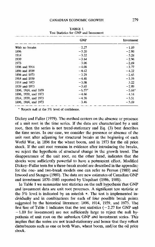
TABLE 1 Test Statistics for GNP and Investment

GNP Investment

With no breaks -2.27 -1.89 1896 -3.20 -2.80 1914 -3.22 -3.28 1939 -3.64 - 2.96 1973 -3.06 - 2.69 1896 and 1914 - 4.08 -3.17 1896 and 1939 -4.62 -4.22 1896 and 1973 -3.29 -2.85 1914 and 1939 -4.48 -3.59 1914 and 1973 -3.08 -3.22 1939 and 1973 -3.65 -2.89 1896, 1914, and 1939 -6.57* - 5.66% 1896, 1939, and 1973 -4.66 -4.14 1914, 1939, and 1973 -4.56 -3.51 1896, 1914, and 1973 -3.46 -3.69

* Rejects null at the 5% level of confidence.

Dickey and Fuller (1979). The method centers on the absence or presence of a unit root in the time series. If the data are characterized by a unit root, then the series is not trend-stationary and Eq. (3) best describes the time series. In our case, we consider the presence or absence of the unit root after adjusting for structural breaks at the beginning of each World War, in 1896 for the wheat boom, and in 1973 for the oil price shock. If the unit root remains in evidence after introducing the breaks, we reject the hypothesis of structural change in the growth trend. The disappearance of the unit root, on the other hand, indicates that the shocks were sufficiently powerful to have a permanent effect. Modified Dickey-Fuller tests for a three-break model are described in the appendix; for the one- and two-break models one can refer to Perron (1989) and Inwood and Stengos (1989). The data are new estimates of Canadian GNP and investment 1870-1985 reported by Urquhart (1986, 1988).

In Table 1 we summarize test statistics on the null hypothesis that GNP and investment data are unit root processes. A significant test statistic at the 5% level is indicated by an asterisk *. The test is implemented in- dividually and in combinations for each of four possible break points suggested by the historical literature: 1896, 1914, 1939; and 1973. The first line of Table 1 indicates that the test statistics (- 2.27 for GNP and - 1.89 for investment) are not sufficiently large to reject the null hyL pothesis of unit root on the unbroken GNP and investment series. This implies that the series are not trend-stationary and hence that they reflect disturbances such as one or both Wars, wheat boom, and/or the oil price shock.

280 INWOOD AND STENGOS

The effect of introducing structural breaks for these events, individually and in combination, is represented in the remainder of Table 1. For GNP, for example, the second line shows the effect of recognizing one structural break at the onset of the wheat boom in 1896; the test statistic rises to -3.20, but remains too small for a rejection of the null hypothesis. In other words, the data continue to show evidence of exogenous shocks with permanent impact even after adjusting for a structural break in 1896.

The remaining lines of Table 1 indicate that only the three-break scen- ario involving wheat boom and two Wars raises the GNP test statistic above its critical value of -5.13 (appendix). A similar pattern is obtained in the case of investment. A straightforward interpretation of this pattern is that the wheat boom and both Wars changed the growth process in the sense of altering the underlying trend by which GNP and investment expanded. The rejection of a unit root after introducing the three breaks also implies that the data are now trend-stationary, and hence that there are no other exogenous shocks with permanent impact. By implication, therefore, neither of the two great depressions (1870s and 1930s) nor the 1973 oil shock can be viewed as an exogenous shock responsible for a change in the trend rate of growth.

IV. CONCLUSIONS

The test statistics support a straightforward characterization of growth between 1870 and 198.5. The Canadian economy grew with its own internal dynamic, as represented in a deterministic growth model with a stationary stochastic term (such as Eq. (1)). Growth was influenced by various ex- ogenous shocks. Some shocks took GNP and investment away from their trends on a merely transitory basis. The wheat boom and both World Wars, by contrast, had an enduring impact in the sense that they changed the underlying growth trend of the economy.

The effect may be illustrated by examining the trends estimated under the assumption of deterministic growth that changed in 1896, 1914, and 1939. The trend rate of annual GNP growth is represented by trend lines in Fig. 1. Annual growth is estimated to be 1.3% until 1896, doubling to 2.7% in the wheat boom era, falling back to 0.8% with the onset of World War One, and rising again to 2.1% in 1939.

The first change in growth trend confirms the belief of an earlier gen- eration of economic historians that the wheat boom marked a major turning point in Canadian development. New national income estimates and improved price data have provided some support for the “disconti- nuity hypothesis,” but the trend-stationarity problem has made it impos- sible to determine if the wheat boom was a temporary deviation from an unchanged growth trend or if the trend itself changed. Our technique permits a formal affirmation of the traditional perspective on the wheat boom and also directs attention at the First World War which appears to

CANADIAN ECONOMIC GROWTH 28

have affected Canada significantly and adversely, in contrast to the Second World War which had a powerful positive effect. The contrasting impact of the two Wars may reflect differences in the state of the economy on the eve of War, as well as characteristics specific to each War and sub- sequent transition to peace.

The analysis also implies something about the depressions of the mid- 1870s and 1930s which were severe in Canada as elsewhere. We cannot assume that the depressions were exogenous to the process of domestic growth. In any case, their impact appears to have been transitory rather than permanent. We know this because trend-stationarity is restored without introducing a break at the onset of the depressions. In the case of the 1930s depression we have taken the further precaution of testing for the disappearance of unit root by introducing three-way breaks 1896--1914- 1929 and 1896-1929-1939. Neither of these combinations suffices to restore trend-stationarity. We conclude that the economy temporarily deviate from its trend during the Great Depression, but that the trend rate of growth did not change.

From a macroeconomic perspective our analysis carries at least two important implications. First, the discovery of a unit root conditions any future choice of techniques for time series modelling on Canadian long- term data. Already it is common to incorporate structural breaks at the outbreak of each World War in econometric analysis. Our analysis indicates that this tendency is more than a methodological convenience; it is required by the problem of trend-stationarity. The powerful exogenous shock as- sociated with the wheat boom also requires a structural break in any model estimated on the period spanning the turn of the century.

A second macroeconomic implication is that if one is willing to extract from the series the exogenous shocks that occurred in 1896, 1914, and 1939, then one can examine the Canadian economy as evolving around a steady trend disturbed by transitory cyclical fluctuations. To the extent that these fluctuations are consistent with theories emphasizing the role of aggregate demand over the role of aggregate supply, the former would seem to be the most relevant for business cycle analysis of the Canadian economy.

In summary, we use an extremely simple growth model in order to determine changes in the trend rate of growth as a result of exogenous shocks. In this specific sense we have tested for structural change in the growth process. We have not considered, however, change in the internal structures of the economy. Indeed, the strength of the technique used in this paper is its generality, since we do not assume anything about the precise structure of relations within the economy. We do conclude, however, that any test for a change in internal structures requires explicit recognition of the turning points in the aggregate pattern of growth identified through the process of restoring trend-stationarity.

282 INWOOD AND STENGOS

APPENDIX: TESTING FOR STRUCTURAL CHANGE IN THE PRESENCE OF A UNIT ROOT AND THREE

EXOGENOUS SHOCKS

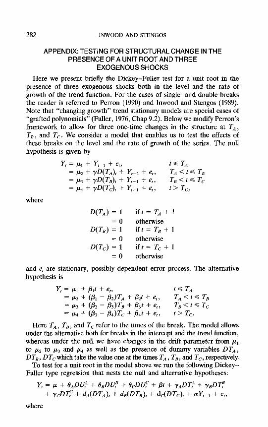
Here we present briefly the Dickey-Fuller test for a unit root in the presence of three exogenous shocks both in the level and the rate of growth of the trend function. For the cases of single- and double-breaks the reader is referred to Perron (1990) and Inwood and Stengos (1989). Note that “changing growth” trend stationary models are special cases of “grafted polynomials” (Fuller, 1976, Chap 9.2). Below we modify Perron’s framework to allow for three one-time changes in the structure at TA, TB, and Tc. We consider a model that enables us to test the effects of these breaks on the level and the rate of growth of the series. The null hypothesis is given by

where

K = PI + X-1 + e,, te TA = ru2 + rDG% + L + et, TA < t s TB = p3 + YW~)~ + JL + et, TB < t G Tc = p4 + YWCL + K-l + et, t’ Tc,

D(T,) = 1 if t = TA + 1 0

D(T,) 1 1 otherwise ift= TB+ 1

0 D(T,) 1 1

otherwise ift= T,+ 1

= 0 otherwise

and e, are stationary, possibly dependent error process. The alternative hypothesis is

K = pt + Pd + et, t =G TA = ~2 + 0% - &)TA + P2t + et, TA < t s TB = ~3 + (P2 - P&b + Pd + et, TB -=c t =s Tc = (u4 + (P3 - &)Tc + Pd + ef, t> Tc.

Here T, , TB , and Tc refer to the times of the break. The model allows under the alternative both for breaks in the intercept and the trend function, whereas under the null we have changes in the drift parameter from pl to ,b to p3 and I(L~ as well as the presence of dummy variables DT,, DT, , DT, which take the value one at the times TA , TB , and Tc , respectively.

To test for a unit root in the model above we run the following Dickey- Fuller type regression that nests the null and alternative hypotheses:

Y, = p + 0,DUf’ + &DUf + &De + /3t + y,DTf + yeDTf + Y&C + &(DTA), + &(DTB), + dXDTc), + ~Y,-I + et,

where

CANADIAN ECONOMIC GROWTH 283

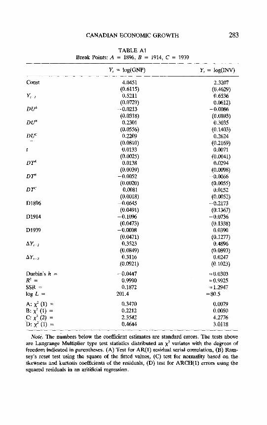
TABLE Al Break Points: A = 1896, B = 1914, C = 1939

Y, = log(GNP) Y, = log(INV)

Const

Y,-*

DUA

DUB

DUC

DP

DTB

DF

D1896

D1914

D1939

AYt-,

AYr-,

Durbin’s h = -9.0447 R* = 0.9990 SSR = 0.1872 log L = 201.4

= 0.0303 = 0.9925 = 1.2947

=80.5

A: x” (1) = 0.3470 0.0079 B: x2 (1) = 0.2212 0.0050 c: x2 (2) = 2.3542 4.2776 D: x” (1) = 0.4644 3.0118

4.0451 (0.6115) 0.5211

(0.0729) -0.0213 (0.0318) 0.2301

(0.0556) 0.2209

(0.0810) 0.0133

(0.0025) 0.0138

(0.0039) -0.0052 (0.0020) 0.0081

(0.0018) -0.0645 (0.0491)

-0.1096 (0.0473)

-0.0008 (0.0471) 0.3523

(0.0849) 0.3116

(0.0921)

2.3207 (0.4629) 0.6536 0.0612)

-0.0086 (0.0893) 0.3035

(0.1403) 0.2624

(0.2169) 0.0071

(0.0041) 0.0294

(0.0098) -0.0066 (0.005s) 0.0152

(0.0052) - 0.2113 (0.1367)

-0.0736 (0.1338) 0.0390

(0.1277) 0.4896

(0.0893) 0.0247

(0.1023)

Note. The numbers below the coefficient estimates are standard errors. The tests above are Langrange Multiplier type test statistics distributed as x2 variates with the degrees of freedom indicated in parentheses. (A) Test for AR(l) residual seriai correlation, (B) Ram- sey’s reset test using the square of the fitted values, (C) test for normality based on the skewness and kurtosis coefficients of the residuals, (D) test for ARCH(l) errors using the squared residuals in an aritificial regression.

284 INWOOD AND STENGOS

DU;’ = 0 if t s TA = 1 TA < t 4 TB =o t> TB

DlJf=O if t G TB = 1 TB < t =s Tc

0 D&O

ift> Tc ift< Tc

1 Or;‘:0

ift> Tc if t G TA

= t - TA TA < t =s TB = 0 t> TB

DT; = 0 ift< TB =t-T,T,<t=sT,

0 D&O

ift> Tc ifts Tc

= t - Tc ift> Tc.

In order to introduce the errors e, in the Dickey-Fuller regressions to be independent one adds AYf-i terms in these regressions to remove any possible correlation of the errors. Both the autocorrelation function of the residuals and the Langrange Multiplier test statistic of no serial correlation were used to determine how many of these terms to add. In the regressions we considered two such terms were sufficient to induce white noise residuals, see Table Al.

To obtain the critical values we conduct a Monte Carlo simulation since the values tabulated by Perron are only applicable in the case of one break in our model. We generate a unit root series with no drift and iid errors and simulate the t ratios in the various models with actual sample size and the actual breaks in the model. Since each model with different break points yields different critical values we use the maximum of the computed critical values. The maximum of the critical values computed for the two-break model is -4.8555 and for the three-break model it is -5.1316 at the 5% level of significance after performing 2000 replications. Regression results for the three-break model (1896, 1914, and 1939) are reported in Table Al. Results with the other break points are available from the authors.

REFERENCES Altman, M. (1987), “A Revision of Canadian Economic Growth: 1870-1910.” Canadian

Journal of Economics 20. Bertram, G. (1963), “Economic Growth and Canadian Industry, 1870-1915: The Staple

Model and the Takeoff Hypothesis.” Canadian Journal of Economics and Political Science 29.

CANADIAN ECONOMIC GROWTH 28.5

Chambers, E. J. (1964), “Late Nineteenth Century Business Cycles in Canada.” Canadian Journal of Economics and Political Science 30.

Chambers, E. J., and Gordon, D. F. (1966), “Primary Products and Economic Growth: An Empirical Measurement.” Journal of Political Economy 74.

Crafts, N., Leybourne, S. and Mills, T. (1989), “The Climacteric in Late Victorian Britain and France: A Reappraisal of the Evidence.” Journal of Applied Economics 4.

Dickey, D. A., and Fuller, W. A. (1979), “Distribution of the Estimators for Autoregressive Time Series with a Unit Root.” Journal of the American Statistical Association 74,

Durlauf, S. N., and Phillips, P. C. B. (1988), “Trends Versus Stationary Walks in Time Series Analysis.” Econometrica 56.

Drummond, I. M. (1986), “Economic History and Canadian Economic Performance since the Second World War.” In J. Sargent (Ed.), Postwar Macroeconomic Developments. Toronto: Univ. Toronto Press.

Fuller, W. A. (1976), Introduction to Time Series. New York: Wiley. Goldin, C., and Margo, R. “Wages, Prices and Labor Markets before the Civil War.”

NBER Working Paper No. 3198. Green, A. G., and Urquhart, M. C. (1987), “New Estimates of Output Growth in Canada:

Measurement and Interpretation.” In D. McCalla (Ed.), Perspectives on Canadian Economic History. Toronto: Copp Clark Pitman.

Harley, C. K. (1986), “Resources and Economic Development in Historical Perspective.” In D. Laidler (Ed.), Resources and Economic Development in Historical Perspective. Toronto: Univ. Toronto Press.

Hartland, P. (1955), “Factors in Economic Growth in Canada.” Journal oJ?&onomic History 15.

Hausman, W., and Watts, J. (1980), “Structural Change in the 18th~Century British Economy: A Test Using Cubic Splines.” Explorations in Economic History 17.

Hay, K. A. J. (1966), “Early Twentieth Century Business Cycles in Canada.” Canadian Journal of Economics and Political Science 32.

Hay, K. A. J. (1967), “Money and Cycles in Post-Confederation Canada.” Journal of Political Economy 75.

Inwood, K., and T. Stengos (1989), “Structural Change and Canadian Economic Growth, 1870-1939.” University of Guelph, Department of Economics Working Paper 89-9.

McDougall, D. (1971), “Canadian Manufactured Commodity Output, 1870-1915.” Canadian Journal of Economics 4.

McDougall, D, (1973), “The Domestic Availability of Manufactured Commodity Output, Canada, 1870-1915.” Canadian Journal of Economics 6.

Naylor, R. T. (1981), “The Canadian State, the Accumulation of Capital, and the Great War.” Journal of Canadian Studies 16.

Nelson, C. R., and Plosser, C. I. (1982), “Trends and Random Walks in Macroeconomic Time Series.” Journal of Monetary Economics 10.

Perron, P. (1988), “Trends and Random Walks in Macroeconomic Time Series: Further Evidence from a New Approach.” Journal of Economic Dynamics and Control l2,

Perron, P. (1989), “The Great Crash, the Oil Price Shock and the Unit Root Hypothesis.” Econometrica 57.

Prescott, E. (1987). ‘*Theory ahead of Business Cycle Measurement.” Carnegie-Mellon Conference on Public Policy.

Safarian, E. (1970) The Canadian Economic during the Great Depression. Toronto: McClelland and Stewart.

Stock, J., and Watson, M. (1988), “Variable Trends in Economic Time Series.” Journal of Economic Perspectives 2.

Urquhart, M. C. (1986) “New Estimates of Gross National Product, Canada, 1870-1926:

286 INWOOD AND STENGOS

Some Implications for Canadian Development.” In S. Engerman and R. Gallman (Eds.), Long-Temz Factors in American Economic Growth. Chicago: Univ. Chicago Press and the National Bureau of Economic Research.

Urquhart, M. C. (1988), “Canadian Economic Growth 1870-1980.” Queen’s University Institute of Economic Research, Discussion Paper 734.

Wasserfallen, W. (1986), “Non-stationarities in Macro-economic Time Series: Further Evidence and Implications.” Canadian Journal of Economics 19.