Embed Size (px)
Citation preview

2009 Copyright 2009 ©Andreas Spanias I-1
Digital Signal ProcessingFundamentals with Hands-on Experiments
by
Andreas Spanias, Ph.D.
June 24, 2009School of Electrical, Computer and Energy Engineering
Arizona State UniversityTempe, AZ 85287-5706
480 965 1837480 965 8325
DSP Primer – June 24, 2009Sponsored in part by NSF 0817596
2009 Copyright 2009 ©Andreas Spanias I-2
Disclaimer
These course notes cover the fundamentals and select applications of Digital Signal Processing and are intended solely for education. No other use is intended or authorized. No warranty or implied warranty is given that any of the material is fit for a particular purpose, application, or product. Although the author believes that the concepts, algorithms, software, and data presented are accurate, he provides no guarantee or implied guarantee that they are free of error. The material presented should not be used without extensive verification. If you do not wish to be bound by the above then please do not use these notes.
2009 Copyright 2009 ©Andreas Spanias I-3
Contents
• Introduction to DSP - Review of analog signals and sampling
• Discrete-time systems and digital filters• The z transform in DSP• Design of FIR digital filters• Design of IIR digital filters• The discrete and the fast Fourier
transform• FFT info and applications
2009 Copyright 2009 ©Andreas Spanias I-4
Digital Signal Processing (DSP) Introduction
• Digital Signal Processing (DSP) is a branch of signal processingthat emerged from the rapid development of VLSI technology that made feasible real- time digital computation.
• DSP involves time and amplitude quantization of signals and relies on the theory of discrete- time signals and systems.
• DSP emerged as a field in the 1960s.
• Early applications of off- line DSP include seismic data analysis, voice processing research.
2009 Copyright 2009 ©Andreas Spanias I-5
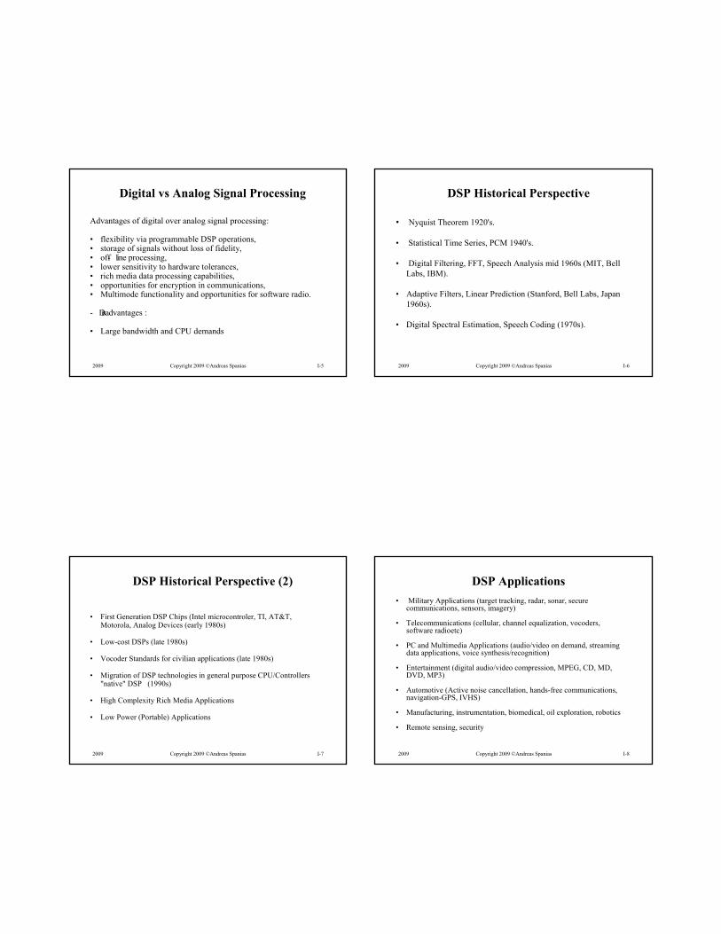
Digital vs Analog Signal Processing
Advantages of digital over analog signal processing:
• flexibility via programmable DSP operations,• storage of signals without loss of fidelity,• off- line processing,• lower sensitivity to hardware tolerances,• rich media data processing capabilities,• opportunities for encryption in communications,• Multimode functionality and opportunities for software radio.
- Disadvantages :
• Large bandwidth and CPU demands
2009 Copyright 2009 ©Andreas Spanias I-6
DSP Historical Perspective
• Nyquist Theorem 1920's.
• Statistical Time Series, PCM 1940's.
• Digital Filtering, FFT, Speech Analysis mid 1960s (MIT, Bell Labs, IBM).
• Adaptive Filters, Linear Prediction (Stanford, Bell Labs, Japan 1960s).
• Digital Spectral Estimation, Speech Coding (1970s).
2009 Copyright 2009 ©Andreas Spanias I-7
DSP Historical Perspective (2)
• First Generation DSP Chips (Intel microcontroler, TI, AT&T, Motorola, Analog Devices (early 1980s)
• Low-cost DSPs (late 1980s)
• Vocoder Standards for civilian applications (late 1980s)
• Migration of DSP technologies in general purpose CPU/Controllers"native" DSP (1990s)
• High Complexity Rich Media Applications
• Low Power (Portable) Applications
2009 Copyright 2009 ©Andreas Spanias I-8
DSP Applications
• Military Applications (target tracking, radar, sonar, secure communications, sensors, imagery)
• Telecommunications (cellular, channel equalization, vocoders, software radioetc)
• PC and Multimedia Applications (audio/video on demand, streamingdata applications, voice synthesis/recognition)
• Entertainment (digital audio/video compression, MPEG, CD, MD, DVD, MP3)
• Automotive (Active noise cancellation, hands-free communications, navigation-GPS, IVHS)
• Manufacturing, instrumentation, biomedical, oil exploration, robotics
• Remote sensing, security

2009 Copyright 2009 ©Andreas Spanias I-9
Communications and DSP
• DTMF (use of the FFT and digital oscillators)
• Adaptive echo cancellation (Hands-free telephony, Speakerphones)
• Speech coding (speech coding in cellular phones)
• Modem (data/computer connectivity)
• Software radio (multi-mode/multi standard wireless communications)
• Channel estimation (equalization)
• Antenna beamforming (space division multiple access - SDMA)
• CDMA (modulating with random sequences)
2009 Copyright 2009 ©Andreas Spanias I-10
Typical Digital Signal Processing System
x(t) x`(t) x(nT)
y(nT)
y`(t)y(t)
LPF sample& A/D
Digital Signal Processor
D/ALPF
fs
Remarks: The diagram shows the sampling, processing, and reconstruction of an analog signal. There are applications where processing stops at the digitalsignal processor, e.g., speech recognition.
AntialiasingReconstruction
NowdaysNowdays LPF and A/D integratedLPF and A/D integrated
NowdaysNowdays LPF and D/A integratedLPF and D/A integrated
DSP chip
2009 Copyright 2009 ©Andreas Spanias I-11
Symbols and Notation
indextimediscrete;
function)(systemresponseimpulse;(.)
functionsresponsefrequencyandtransfer;(.)
outputtimediscrete;)(
inputtimediscrete;)()(|)(
n
h
H
ny
nxnTxtx nTta
Remarks: In general and unless otherwise stated lower case symbols will be used for time-domain signals and upper case symbols will be used fortransform domain signals. Bold face or underlined face symbols will be Be generally used for vectors or matrices.
2009 Copyright 2009 ©Andreas Spanias I-12
Continuous vs Discrete-time
Remarks: A continuous-time signal is converted to discrete-time using sampling and quantization. As a result aliasing and quantization noise is introduced. This noisecan be controlled by properly designing the quantizer and anti-aliasing filter.
Qx(t) x(n)
t
x(t)
n
Continuous-time (analog) Signal Discrete-time (digital) signal
0 T 2T ...
x(n)

2009 Copyright 2009 ©Andreas Spanias I-13
Quantization Noise
sampling period
)()()( tetxtx qq
eq(t)
analog waveform
quantized waveform
quantization noise
T
xa(t)
xq(t)
2009 Copyright 2009 ©Andreas Spanias I-14
Simplest Quantization Scheme -Uniform PCM
Performance in terms of Signal to Noise Ratio (SNR)
where Rb is the number of bits and the value of K1
depends on signal statistics. For telephone speechK1 = -10
1bPCM KR02.6SNR
2009 Copyright 2009 ©Andreas Spanias I-15
Oversampling / or / Conversion
• Integrated oversampling and 1-bit quantization
• Very compact and inexpensive circuitry (some low power applications as well)
• Lowers analog circuit complexity with a modest increase in software (DSP MIPS) complexity
• Uses concepts from multirate signal processing and Delta Modulation
• Will be described in the context of multirate signal processing
2009 Copyright 2009 ©Andreas Spanias I-16
Time vs Frequency Domain
t f0 0
...
. . .. . .
t
x ( t )
t im e -d o m a in fr e q u e n c y -d o m a in
|X ( f ) |
f
...
. . .
0 0
.. .
x ( t ) |X ( f ) |
Remarks: Slowly time-varying signals tend to have low-frequency contentwhile signals with abrupt changes in their amplitudes have high frequency content.The frequency content of signals can be estimated using Fourier techniques.

2009 Copyright 2009 ©Andreas Spanias I-17
Example: Time vs Frequency Domain Speech
Time domain speech segment
Time (mS)
Am
plit
ud
e
TAPE TIME: 3840
0 8 16 24 32
1.0
0.0
-1.0
Ma
gn
itu
de
(d
B)
-30
0
20
40
0 1 2 3 4
Frequency (KHz)
Time domain speech segment
Time (mS)
Am
pli
tud
e
TAPE TIME: 8014
0 8 16 24 32
1.0
0.0
-1.0
Mag
nit
ud
e (
dB
)
-20
0
20
50
0 1 2 3 4
Frequency (KHz)
fundamental
frequency
Formant Structure
Periodic waveform gives harmonic spectraPeriodic waveform gives harmonic spectra
2009 Copyright 2009 ©Andreas Spanias I-18
Some Important Signals
)(n ....
n
1
0
Discrete-time Impulse
Think of signals as a weighted sum of impulses. Think of signals as a weighted sum of impulses. Impulses help in analyzing signals and filtersImpulses help in analyzing signals and filters
2009 Copyright 2009 ©Andreas Spanias I-19
Some Important Signals (3)
Sinusoids are used in analyzing or synthesizing acoustic and othSinusoids are used in analyzing or synthesizing acoustic and other signalser signals
The sinusoid
)2
(sin)(sin tT
t
Period TPeriod T
Tf
22 units: units: ωω((rad/srad/s) ) f f (Hz) T(s)(Hz) T(s)
2009 Copyright 2009 ©Andreas Spanias I-20
Some Important Signals (4)
The sinc function
t
tt
)sin()(sinc
. . .
0
. . .
π 2π
SincSinc functions often appear in signal and filter analysisfunctions often appear in signal and filter analysisparticularly when considering frequency domain behaviorparticularly when considering frequency domain behavior
mainlobemainlobesidelobessidelobes

2009 Copyright 2009 ©Andreas Spanias I-21
Some Important Signals (5)
Random noise
Encountered in communication systems and other applicationEncountered in communication systems and other applicationCharacterized by their mean and varianceCharacterized by their mean and variance
2009 Copyright 2009 ©Andreas Spanias I-22
Representing Periodic Signals with Sinusoids
)sin()cos( tkjtke ootjk o
11
0 )sin()cos()(k
okk
ok tkbtkaatx
k
tjkk
oeXtx )(
Fourier series: Trigonometric form:Fourier series: Trigonometric form:
Fourier series: Complex (magnitude/phase) form:Fourier series: Complex (magnitude/phase) form:
Preferred in engineering Preferred in engineering - -- - >>>>
Xk are complex F.S. coefficients and provide spectral magnitude andare complex F.S. coefficients and provide spectral magnitude and phase infophase info
andand
2009 Copyright 2009 ©Andreas Spanias I-23
Fourier Series Analysis ExampleRepresenting a Periodic Pulse Train as a Sum of Harmonic Sinusoids
Remarks: A periodic pulse signal has a discrete F.S. spectrum described bysamples that fall on a sinc (sinc(x)=sin(x)/x) function. As the period increases the F.S. components become more dense in frequency and weaker in amplitude. If T goes to infinity periodicity is lost and the F.S. vanishes.
. . . . . .
T
d
0 t
x ( t )
2sinc1
1 2/
2/
dk
T
ddte
TX o
d
d
tjkk
o
2009 Copyright 2009 ©Andreas Spanias I-24
Fourier Series Example (2)Harmonic Spectrum
. . . . . .
0
Fundamental frequency o
o2
kX
4/1T
d
o3harmonics

2009 Copyright 2009 ©Andreas Spanias I-25
d/T=1/5
d/T=1/10
4π
2π
0
0
Fourier Series Example (3)
2009 Copyright 2009 ©Andreas Spanias I-26
Use Sinusoids to synthesize a periodic pulse using the Fourier series (only one period shown)
1 sinusoid1 sinusoid
2 sinusoids2 sinusoids
3 sinusoids3 sinusoids
10 sinusoids10 sinusoids
50 sinusoids50 sinusoids
100 sinusoids100 sinusoids
2009 Copyright 2009 ©Andreas Spanias I-27
The Continuous Fourier Transform (CFT) Equations
The Fourier transform
dtetxX tj )()(
The inverse Fourier transform
1( ) ( )
2j tx t X e d
A Fourier transform pair is designated by: )()( Xtx
Synthesis Expression
Analysis Expression
Remarks: Both time and frequency are continuous variables. The CFT canhandle non-periodic signals as long as they are integrable. Periodic signals can be handled using the impulse and CFT properties.
2009 Copyright 2009 ©Andreas Spanias I-28
2sinc)(
2/
2/
dddteX
d
d
tj
Fourier transform of a time-limited pulse(Represent a single pulse by sinusoids)
Given the signal tx
d
t......
0
Remarks: Note that a time-limited signal has a non-bandlimited CFT spectrum.The sinc function has zero crossings at integer multiples of 2π/d. As the pulsewidth increases the sinc function “shrinks”. In the limit, if T goes to infinity (i.e., pulse becomes D.C. signal) the sinc function collapses to a unit impulse.

2009 Copyright 2009 ©Andreas Spanias I-29
Fourier transform of a time-limited pulse(Cont.)
. . .
0
. . .
2sinc)(
ddX
ω
2π /d 4π/d
d
t...... . . .
0
. . .
a transform paira transform pairtime domaintime domain frequency domainfrequency domain
pulsepulse sincsinc
2009 Copyright 2009 ©Andreas Spanias I-30
Symmetry of the Fourier transform
)(2)()()( xtXthenXtxif
t...... . . .
0
. . .
. . .
0
. . . ......
t
x(t)
X(t)
X(ω)
2π x(-ω)
(time(time--limited)limited)
(band(band--limited)limited)(non time(non time--limited)limited)
(non band(non band--limited)limited)
2009 Copyright 2009 ©Andreas Spanias I-31
The Time-Domain Convolution (Filtering) Property
)()(
)()(
Hth
Xtx
DEMODEMO
)()()(*)( XHtxth
convolution in time is multiplication in frequencyconvolution in time is multiplication in frequency
dtxhtxth )()()(*)(
......t
... ...... * = t
Example: Convolution of an exponential with a pulseExample: Convolution of an exponential with a pulse
MuliplicationMuliplication in frequency in frequency is essentially a filtering operationis essentially a filtering operation
2009 Copyright 2009 ©Andreas Spanias I-32
))()(()cos( 000 t
Important Fourier Transform Pairs
tω
ωO0-ωO
π(ω- ωO)

2009 Copyright 2009 ©Andreas Spanias I-33
Truncating a Cosine
t
1
0T
0( ) cos( )s t t 0 0( ) ( ( ) ( ))S
ω000
CFT
0 0where 2 /T
0
t
1
0T
( ) ( ) ( )ws t s t w t
0T
ω000
CFT
0
( )w t
0 / 20 0 0 0 0( ) sinc / 2 +sinc / 2j T
wS T e T T
01; 0( )
0; otherwise
t Tw t
CFT0 / 2
0( ) sinc2
j T 0TW T e
2009 Copyright 2009 ©Andreas Spanias I-34
Truncating Signals with Tapered Windows
....
t
.. .. t
25dB
13dB
B
1.33B
… …
… …
2009 Copyright 2009 ©Andreas Spanias I-35
Truncating Speech
CFT
Normalized frequency x rad/sec
2009 Copyright 2009 ©Andreas Spanias I-36
CFT
Normalized frequency x rad/sec
Truncating Speech (tapered window)

2009 Copyright 2009 ©Andreas Spanias I-37
The Sampling Process
A bandlimited signal that has no spectral components at or above B can be uniquely represented by its sampled values spaced at uniform intervals that are not more than π/B seconds apart.
or a signal that is bandlimited to B must be sampled at a rate of ωs where
BT
xx ==analog signalanalog signal samplingsampling digital signaldigital signal
B
forB ss 2
2009 Copyright 2009 ©Andreas Spanias
Example: Audio - Bandwidth
200 - 3200 Hz Basic Telephone SpeechIntelligiblePreserves Speaker Identity
50 - 7000 Hz Wideband SpeechAM-grade audio
50 - 15000 Hz Near High FidelityFM-grade Audio
20 - 20000 Hz High-FidelityCD/DAT Quality Voice
2009 Copyright 2009 ©Andreas Spanias
Example: Sampling of Audio Signals
192 kHz96 kHzDVD audio (DVD-A)
2.8224 MHz100 kHzSuper audio CD
(SACD)
48 kHz20 kHzDigital audio tape
(DAT)
44.1 kHz20 kHzHigh-fidelity, CD
16 kHz7 kHzWideband audio
8 kHz3.2 kHzTelephony
Sampling frequencyBandwidthFormat
2009 Copyright 2009 ©Andreas Spanias I-40
Sampling and Periodic Spectra
......
……
t 00
)(tx )(X
BB
... ...
T 2T 3T
......
0
)(txs
0
)(sX
B ss2s Bt
1/T

2009 Copyright 2009 ©Andreas Spanias I-41
Signal Reconstruction using an Ideal Filter
... ...
T 2T 3T
......
0
)(txs
0
)(sX
B s s2s Bt
1/T
......
……
t 00
)(tx )(X
BB
T
2009 Copyright 2009 ©Andreas Spanias I-42
ALIASING (UNDERSAMPLING) ωs<2B
the signal can not be recovered perfectly even with an ideal filthe signal can not be recovered perfectly even with an ideal filter ter only a distorted version of the signal can be recoveredonly a distorted version of the signal can be recovered
......
0
)(sX
B s s2B
aliasingaliasing
2009 Copyright 2009 ©Andreas Spanias I-43
Oversampling ωs>>2B
...
0
)(sX
B s s2s B
Guard bandsGuard bands
OversamplingOversampling relaxes the requirements on relaxes the requirements on antialiasingantialiasing filtersfilters
It is used in It is used in // ((/ / ) A) A--toto--D convertersD converters
2009 Copyright 2009 ©Andreas Spanias I-44
Example
Differential equation:
dy t
dt RCy t
RCx t
( )( ) ( )
1 1
Transfer function:
H ssRC
( )
1
1
x(t)
R
Ci(t) y(t)
Frequency response function:
RCjH
1
1)(
)sin()( ttx then
))(sin()()( HtHty ss
if sinusoid in sinusoid in sinusoid outsinusoid out

2009 Copyright 2009 ©Andreas Spanias I-45
Example - Impulse Response
Consider the circuit below with R=1M, C=1x10⁻⁶
dh t
dt RCh t
RCt
( )( ) ( )
1 1
The solution: h tRC
e et
RC t( ) 1
for t > 0
x(t)
R
Ci(t) y(t)
..
t2009 Copyright 2009 ©Andreas Spanias I-46
Example - Convolve and obtain an output
Consider the RC with impulse response
and the input x t u t u t( ) ( ) ( ) 1
)()( tueth t
1for )(
10for 1)(
)1(
1
0
teedety
tedety
ttt
t
tt
....t
....t
.. ....* =
t

Jan. 2009 Copyright 2009 ©Andreas Spanias II- 1
Discrete-time Linear Systems
Digital Filters
Jan. 2009 Copyright 2009 ©Andreas Spanias II- 2
Discrete- time Linear Systems – Digital Filters
x(n)h(n)
y(n)
The output is produced by convolving the input with the impulse response
)(*)()()()( nxnhmnxmhnym
This operation can also involve a finite-length impulse response(FIR) sequence
L
m
mnxmhny0
)()()(
An FIR filter is programmed using a multiply-accumulate instruction
Jan. 2009 Copyright 2009 ©Andreas Spanias II- 3
Some Definitions
•A digital filter is linear if it has the property of generalized superposition
•A digital filter is causal if it non anticipatory, i.e., the present output does not depend on future inputs.
•All real-time systems are causal.
• Non-causalities arise in image processing where the signal indexes are spatial instead of temporal.
• Unless otherwise stated all systems in this course will be assumed causal.
Jan. 2009 Copyright 2009 ©Andreas Spanias II- 4
Some More Definitions
Lb
.
1zT or ;unit delayx(n) x(n-1)
x(n) bL x(n)
x(n)
x(n-1)
x(n)+x(n-1)
;signal scaling by a filter coefficient
;signal addition
x(n) x(n-1)

Jan. 2009 Copyright 2009 ©Andreas Spanias II- 5
IIR Digital Filter Structure
M
ii
L
ii inyainxbny
10
)()()(
feedback
ny nx
T
1a
Ma0b
Lb... ...
...
.......
- --
1b 2a.
T T T T
Jan. 2009 Copyright 2009 ©Andreas Spanias II- 6
FIR Digital Filter Structure
L
ii inxbny
0
)()(
ny nx
T T
0b
Lb...
.....
1b.
Jan. 2009 Copyright 2009 ©Andreas Spanias II- 7
Two i/p- o/p Equations for Digital Filters
x(n)h(n)
y(n)
One can compute the output using the convolution sum
mm
mnhmxmnxmhny )()()()()(
or by using the difference equation
M
ii
L
ii inyainxbny
10
)()()(
Remark: The impulse response h(n) can be determined by solving the difference equation.
Jan. 2009 Copyright 2009 ©Andreas Spanias II- 8
Unit Impulse
The analysis of digital filters in the frequency domain is facilitatedusing sinusoids. In the time domain a unique input signal is usedfor analysis, namely the unit impulse. That is defined as:
0n for 1elsewhere 0
n
n
n0

Jan. 2009 Copyright 2009 ©Andreas Spanias II- 9
Signal Representation with Unit Impulses
Any discrete-time signal may be represented by a linear combinationof unit impulses
is represented by:
x n n n n
n n n
( ) . ( ) . ( ) ( )
( ) . ( ) . ( )
5 2 1 5 1 2
1 5 2 2 5 3
nx
n10 2 3 4 5
50.
251.
50.
52.1
Jan. 2009 Copyright 2009 ©Andreas Spanias II- 10
Impulse Response
The response of a digital filter to a unit impulse is known as impulse response and is given by
)(...)2()1(
)(...)1()()(
21
10
Mnhanhanha
Lnbnbnbnh
M
L
(n)h(n)
h(n)
Jan. 2009 Copyright 2009 ©Andreas Spanias II- 11
Impulses as input to source- system LPC Vocoders
Vowels are typically synthesized by exciting a filter representiVowels are typically synthesized by exciting a filter representing the ng the mouth and nasal (vocal tract) cavity with a train of periodic immouth and nasal (vocal tract) cavity with a train of periodic impulsespulses
VOCAL
TRACT
FILTER
SYNTHETIC
SPEECH
gain
i
innx )()( pitch periodpitch period
TimeTime--varyingvaryingdigital filterdigital filter
Jan. 2009 Copyright 2009 ©Andreas Spanias II- 12
Finite- Length Impulse Response (FIR)
If the digital filter has no feedback terms the impulse response isfinite length
)(...)1()()( 10 Lnbnbnbnh L
0)0( bh
1)1( bh
2)2( bh
LbLh )(
..
..
Note that
Remark: The filter has a finite-length impulse response and is called FIR. The values of the impulse response sequence are the coefficients themselves. The filter is always stable.

Jan. 2009 Copyright 2009 ©Andreas Spanias II- 13
Example – The Moving Average Filter
)(...)1()(1
1)( Lnnn
Lnh
LnL
nh
01
1)(
Remark: The moving average is essentially a low-pass (smoothing) filter. Later on we will see that this filter is also optimal in estimation problems.
L
i
inxL
ny0
)(1
1)(
Jan. 2009 Copyright 2009 ©Andreas Spanias II- 14
J-DSP Simulation of Averaging Filter
L=10 L=50
Jan. 2009 Copyright 2009 ©Andreas Spanias II- 15
Infinite- Length Impulse Response (IIR)
If the digital filter has feedback terms then the impulse response is infinite length
M
ii
L
ii inhainbnh
10
)()()(
Example: )1()()( 1 nhannh
1)0( h 1)1( ah 21)2( ah .... nanh )()( 1
Remark: Note that if the coefficient a1 has magnitude larger than one the impulse response will go to infinity and hence the filter would be unstable.
Jan. 2009 Copyright 2009 ©Andreas Spanias II- 16
IIR – Another First Order Example
)1(8.0)(2.0)( nhnnh
0)8.0(2.0)( nnh n
nh
1z
8.0
n
2.0
Remark: This particular IIR filter is also a low-pass filter behaving in similar manner like the the averaging FIR filter.

Jan. 2009 Copyright 2009 ©Andreas Spanias II- 17
IIR – Another First Order Example (Plot)
0 5 10 15 20 250
0.02
0.04
0.06
0.08
0.1
0.12
0.14
0.16
0.18
0.2
0)8.0(2.0)( nnh n
Jan. 2009 Copyright 2009 ©Andreas Spanias II- 18
Frequency Responses
11 z
π Ω π Ω
π Ωπ Ω
11 z
)9.01( 1 z )9.01( 1 z
dB dB
dB dB
0 0
( )jH e
11
( )jH e
0 0
11 z
π Ω π Ω
π Ωπ Ω
11 z
)9.01( 1 z )9.01( 1 z
dB dB
dB dB
0 0
( )jH e
11
( )jH e
0 0
Jan. 2009 Copyright 2009 ©Andreas Spanias II- 19
Impulse Response and Stability
Bounded Input Bounded Output (BIBO) stability is defined as
0
)(k
kh
The condition above is guaranteed if
1ip for all i = 1, 2, . . . , M
0
)()()(m
mnxmhny
For the causal digital filter
Jan. 2009 Copyright 2009 ©Andreas Spanias II- 20
An Unstable Filter

Jan. 2009 Copyright 2009 ©Andreas Spanias II- 21
Example of Transient and Steady State Response
ny
1z
8.0
nu
2.0
1)8.0(8.0)()()( nsstr nynyny
01)( nnu
0 2 4 6 8 10 12 14 16 18 200
0.10.20.30.40.50.60.70.80.91
Jan. 2009 Copyright 2009 ©Andreas Spanias II- 22
Steady- State Sinusoidal Response ofDigital Filters
A special case of interest is the steady-state response to input sinusoids and is formulated as follows. For the IIR filter
The frequency response function is given by:
jM
Mjj
jLL
jjj
eaeaea
ebebebbeH
...1
...)(
221
2210
M
ii
L
ii inyainxbny
10
)()()(
Jan. 2009 Copyright 2009 ©Andreas Spanias II- 23
Steady- State Sinusoidal Response ofLinear Discrete Systems (Cont.)
The frequency response function is periodic and an example of thesteady state sinusoidal response is given below
if:
)sin()( nnx
then:
))(sin()()( jjss eHneHny
sf
f2 ;normalized frequency
Jan. 2009 Copyright 2009 ©Andreas Spanias II- 24
Example of Steady State Sinusoidal Response
ny
1z
8.0
nx
2.0
)2
sin()2000/5002sin()(n
nnx
The filter is excited by a 500 Hz sinusoid and theSampling rate is 2000Hz.
))8.01
2.0arg(
2sin(|
8.01
2.0|)(
j
n
jnyss
jj
eeH
8.01
2.0)(

Jan. 2009 Copyright 2009 ©Andreas Spanias II- 25
Frequency Response Plot
jj
eeH
8.01
2.0)(
``
0.1
0.5
1
1000 Hz0

Jan. 2009 Copyright 2009 ©Andreas Spanias III-1
The Z-Transform in DSP
Jan. 2009 Copyright 2009 ©Andreas Spanias III-2
The Z- Transform
•The z-transform plays a similar role in DSP as the Laplace transform in analog circuits and systems.
•It provides intuition that is sometimes not evident in time-domain analysis
•Simplifies time-domain operations – time domain-convolution maps to Z-domain multiplication
•Used to define transfer functions
•Could be used to determine responses of systems using a table look-up process
Jan. 2009 Copyright 2009 ©Andreas Spanias III-3
From the Laplace Transform to the Z- Transform
)()( zHsH da
R
C
sRCsHa
1
1)(
ny
1z nx
111
)(
za
bzH o
d
s-domain transfer function z-domain transfer function
Jan. 2009 Copyright 2009 ©Andreas Spanias III-4
The Z- Transform - Definition
Given the signal: )(nx
its Z-transform is X z x n z n
n
( ) ( )
For causal signals, i.e.,
0
)()(n
nznxzX
00)( nfornx

Jan. 2009 Copyright 2009 ©Andreas Spanias III-5
Selected Properties of the Z- Transform
Linearity: if: x n X z( ) ( ) and y n Y z( ) ( )then
x n y n X z Y z( ) ( ) ( ) ( )
Shifting: )()( zXzmnx m
Convolution: )()()(*)( zYzXnynx
Scaling (bandwidth expansion): )/()( azXnxa n Jan. 2009 Copyright 2009 ©Andreas Spanias III-6
Delay of 7 Samples
7( 7) ( )x n z X z
Jan. 2009 Copyright 2009 ©Andreas Spanias III-7
Selected Z- Transform Pairs
Unit-Impulse: ( )n 1
Sinusoids:
1,)cos(21
)sin(0),sin(
21
1
zzz
znn
1,)cos(21
)cos(10),cos(
21
1
zzz
znn
Sampled Unit-Step: 1 01
111, ,n
zz
Exponential Signals: a nz
z az an , ,
0
Jan. 2009 Copyright 2009 ©Andreas Spanias III-8
The Transfer Function
To write the transfer function put the difference equation in the z-domain
x n X z( ) ( ) y n Y z( ) ( )and
M
ii
L
ii inyainxbny
10
)()()(
iM
ii
L
i
ii zzYazzXbzY
10
)()()(
)(zX
1a
Ma0b
Lb... ...
...
.......
- -
-
1b 2a.
1z
)(zY
1z 1z 1z 1z

Jan. 2009 Copyright 2009 ©Andreas Spanias III-9
The Transfer Function (Cont.)
The transfer function H(z) is defined as:
MM
LL
zaza
zbzbb
zX
zYzH
...1
...
)(
)()(
11
110
)1()()()(10
iM
ii
L
i
ii zazYzbzX
iM
ii
L
i
ii
za
zbzH
1
0
1)(
Note that feedbackterms are in the denominator
Jan. 2009 Copyright 2009 ©Andreas Spanias III-10
The Transfer Function and the Impulse Response
It can be shown that a transfer function H(z) is related to the impulse response sequence h(n) by:
0
)()(n
nznhzH
or
h n H z( ) ( )
Convolution maps to multiplications in the z domain
)()()()(*)()( zHzXzYnhnxny
Jan. 2009 Copyright 2009 ©Andreas Spanias III-11
Example: Write the Transfer Function of a First Order IIR Filter
ny
1z
8.0
nx
2.0
Step 1: Write the Difference Equation
)1(8.0)(2.0)( nynxny
Step 2: Transform all signals to the z domain
)()1(
)()()()(1 zYzny
zXnxzYny
Jan. 2009 Copyright 2009 ©Andreas Spanias III-12
Example: Transfer Function of a First Order IIR Filter (cont.)
Step 3: Since z-transform is a linear operation I can write
)(8.0)(2.0)( 1 zYzzXzY
Step 4: Form the ratio Y(z)/X(z) to get the transfer function
8.0
2.0
8.01
2.0
)(
)()(
1
z
z
zzX
zYzH
Note below that the impulse response can be written by inspection of H(z)
8.0||8.0
2.0)()(8.02.0)(
z
z
zzHnunh n

Jan. 2009 Copyright 2009 ©Andreas Spanias III-13
The Transfer Function of FIR Systems
For the FIR filter the transfer function is:
L
i
ii
LL zbzbzbbzH
0
110 ...)(
this is also in agreement with
L
n
nznhzH0
)()(
Note that for FIR filters
LbbbLhhh ,....,,)(),...,1(),0( 10
Jan. 2009 Copyright 2009 ©Andreas Spanias III-14
Equivalent Filter Realizations
1
2
3
+
++
x(n)
y(n)
1.3
0.4
+
z -1
z -1 z -1
z -1
1
2
3
+
+
+z-1
z-1
1.3
0.4
x(n) y(n)
Direct Form 1
Direct Form 2
saves memory
Jan. 2009 Copyright 2009 ©Andreas Spanias III-15
Poles and Zeros of H(z)
In general the transfer function is rational; it has a numerator and a denominator polynomial.
The roots of the numerator and denominator polynomials are called the zeros and the poles respectively.
Pole-zero decompositions of H(z) are quite useful and provide intuition in signal analysis and filter design.
M
ii
L
ii
M
L
pz
zG
pzpzpz
zzzGzH
1
1
21
21
)(
)(
))...()((
))...()(()(
where G is a gain factor
Jan. 2009 Copyright 2009 ©Andreas Spanias III-16
Example: Poles and Zeros of H(z)
8.0
2.0)(
z
zzH • the zero (O) of this transfer function is at z=0
• the pole (X) of this transfer function is at z=0.8
-1 -0.5 0 0.5 1
-1
-0.5
0
0.5
1
Real part
Imag
inar
y pa
rt
XO

Jan. 2009 Copyright 2009 ©Andreas Spanias III-17
Example: Poles- Zeros of a Second Order System
21
21
55.045.01
9025.03435.11)(
zz
zzzH
Note that the filter coefficients are real valued and therefore poles and zeros occur in complex conjugate pairs.
H zz e z e
z e z e
j j
j j
o o
o o( )( . )( . )
( . )( . ). .
95 95
7416 7416
45 45
72 34 72 34
lm
X
X
0
0
polesX zeros0
Re
Jan. 2009 Copyright 2009 ©Andreas Spanias III-18
Poles and Zeros and Stability
The poles are related to the stability of the filter since they are related to the impulse response of the system. In fact, the poles ofFor stability all the poles must be inside the unit circle, that is
1ip for all i = 1, 2, . . . , M
IIR filters may be all-pole or pole-zero and stability is always a concern. FIR or all-zero filters are always stable.
Jan. 2009 Copyright 2009 ©Andreas Spanias III-19
The Frequency Response Function
The transfer function is
MM
LL
zaza
zbzbbzH
...1
...)(
11
110
by evaluating on the unit circle, i.e. for jez
jM
Mj
jLL
jj
eaea
ebebbeH
...1
...)(
1
10
Jan. 2009 Copyright 2009 ©Andreas Spanias III-20
The Frequency Response Function (Cont.)
The frequency response function and is a complex and periodicWith period 2. The normalized frequencies are associated to the sampling frequencies fs by
sf
fT 2
where fs is the sampling frequency and f is any frequency of interest. In practice, one determines the frequency response up to half the sampling frequency (fold-over frequency).
rad rad/s
Sampling period
Sampling frequency

Jan. 2009 Copyright 2009 ©Andreas Spanias III-21
The Frequency Response Function (Cont.)
0 2
0 fs/2 fs
Foldover Frequency
π π
•The frequency response is usually plotted w.r.t. normalized frequencies ()
•The frequency response is periodic with period fs (2 π )
•Since frequencies of interest are up to the bandwidth of the analog signal
the spectrum is usually plotted up to fs/2, ( π ) the foldover frequency
Jan. 2009 Copyright 2009 ©Andreas Spanias III-22
The Frequency Response and Poles and Zeros
The magnitude frequency response function
M
ii
j
L
ii
j
j
pe
eGeH
1
1)(
The phase frequency response function
M
ii
jL
ii
jj peeeH11
)arg()arg())(arg(
Jan. 2009 Copyright 2009 ©Andreas Spanias III-23
•Poles tend to create peaks in the magnitude frequency response
•Zeros tend to create valleys in the magnitude frequency response
•Very selective filters are designed efficiently by placing polesclose to the unit circle
•Sharp notches are achieved efficiently with zeros very close to the unit circle
•A sharp notch in the frequency response needs many poles (high order) if we are restricted to an all-pole filter (not efficient).
•A sharp peak in the frequency response needs many zeros (long or high order FIR) if an all-zero filter is to be used (not efficient).
Remarks on Effects of Poles and Zeros on H(ej)
Jan. 2009 Copyright 2009 ©Andreas Spanias III-24
Magnitude and Phase Response
The magnitude and phase response of
Frequency Index (Theta=2*PI*Index/128)
Ma
gn
itu
de
H(z
)
0.5
1.0
1.5
2.0
0.032 64 96 1280
0 2
0 fs/2 fs
Foldover Frequency
Magnitude ResponseIm
X
0
polesX zeros0
Re
0
X

Jan. 2009 Copyright 2009 ©Andreas Spanias III-25
Zero Locations and Frequency Response
o
o
o
foldover
o
Jan. 2009 Copyright 2009 ©Andreas Spanias III-26
Pole Locations and Frequency Responses
X
X
X
X
As the poles move outwards we get sharper peaks and if the polesare on the unit circle we get an oscillator.
Jan. 2009 Copyright 2009 ©Andreas Spanias III-27
X
X
X
X
transient
f
nn
Bandwidth Expansion Moving poles inwards stabilizes numerically a filter
The scaling property of the zThe scaling property of the z--transform is exploited for bandwidth expansion in LPC transform is exploited for bandwidth expansion in LPC vocodersvocoders
)/()( zHnhn 10
iM
ii
i zazH
1
1
1)/(
exampleexample
Jan. 2009 Copyright 2009 ©Andreas Spanias III-28
Stabilizing a Filter Using Pole Scaling

Jan. 2009 Copyright 2009 ©Andreas Spanias III-29
Computing Filter Responses Using the Inverse Z-Transform
Partial Fractions: Given a the transfer function
MMM
LLL
azaz
bzbzbzH
...
...)(
11
110
for distinct poles write H(z) as:
MM pz
zc
pz
zcczH
...)(
110
Jan. 2009 Copyright 2009 ©Andreas Spanias III-30
Example: Find the Impulse Response of the Filter
61
652 zzzz
zH2
31
21 -z
z-zz
9 zH 8
h n nn n
( ) ,
9
1
28
1
30
z-1
5/6
1/6
x(n) y(n)
+
+
-+
+
z-1
Jan. 2009 Copyright 2009 ©Andreas Spanias III-31
Filter Configurations
+( )X z
1 ( )H z1 ( )H z 2 ( )H z
3 ( )H z
( )Y z
( )X z
1 2 3( ) ( ) ( )H z H z H z( )Y z
Jan. 2009 Copyright 2009 ©Andreas Spanias III-32
Use z transforms to change the filter structure
+1z 1z 1z 1z
1.2
0.32
-+
x(n) y(n)+
1z 1z 1z 1z 1z 1z 1z 1z
1.2
0.32
-+
x(n) y(n)
1z
8.0
1z
1z
8.0
1z
8.0
1z
0.4
1z 1z
8.02.x(n) y(n)
1z
8.0
1z 1z
8.0 8.0
1z 1z
1z 1z
8.0 8.0
1z 1z
8.0 8.0
1z 1z
0.4
1z 1z 1z 1z
8.0 8.02.2.x(n) y(n)
ny1z
8.0
1z
0.4
x n ny1z
8.0
1z
8.0
1z
0.4
x n
=
=

Jan. 2009 Copyright 2009 ©Andreas Spanias III-33
J-DSP Simulation
Jan. 2009 Copyright 2009 ©Andreas Spanias III-34
Interesting Transfer FunctionsLong Term Prediction Synthesis Filter
pp za
zH
1
1)(
•Called long term because p is a long-term delay•Used in Vocoders
109.01
1)(
zzH
0 0.1 0.2 0.3 0.4 0.5 0.6 0.7 0.8 0.9 1-100
-50
0
50
100
Normalized frequency (Nyquist == 1)
Pha
se (
degr
ees)
0 0.1 0.2 0.3 0.4 0.5 0.6 0.7 0.8 0.9 1-10
0
10
20
Normalized frequency (Nyquist == 1)
Mag
nitu
de R
espo
nse
(dB
)
Example p=10>>
Jan. 2009 Copyright 2009 ©Andreas Spanias III-35
3095.01
1 z
Impulse response
LTP excited by a random signal
0 0.1 0.2 0.3 0.4 0.5 0.6 0.7 0.8 0.9 1-100
-50
0
50
100
Normalized frequency (Nyquist == 1)
Ph
as
e (
de
gre
es
)
0 0.1 0.2 0.3 0.4 0.5 0.6 0.7 0.8 0.9 1-10
0
10
20
Normalized frequency (Nyquist == 1)
Ma
gn
itu
de
Re
sp
on
se
(d
B)
Frequency response
Jan. 2009 Copyright 2009 ©Andreas Spanias III-36
J- DSP Simulation of LTP
10
1( )
1 0.9H z
z

Jan. 2009 Copyright 2009 ©Andreas Spanias III-37
Interesting Transfer FunctionsAll- Pole Filters
Typically used in speech processing(vocoders) as well as in spectral estimation applications
iM
ii
o
za
bzH
1
1)(
T T T
a1
a2
aM
y(n)
-
--
+x(n)b
0
Jan. 2009 Copyright 2009 ©Andreas Spanias III-38
VOCAL
TRACT
FILTER
SYNTHETIC
SPEECH
gain
Interesting Transfer FunctionsAll- Pole Filters (2)
iM
ii za
bzH
1
0
1)(
Jan. 2009 Copyright 2009 ©Andreas Spanias III-39
Interesting Transfer FunctionsDigital Oscillators
If we realize the z-transform of a sinusoid as a transfer function andwe excite it with a unit impulse we get a sinusoidal output
1,)cos(21
)sin(0),sin(
21
1
zzz
znn
21
1
)cos(21
)sin()(
zz
zzH
If we excite H(z) below
with (n) then the output will be a sinusoid
Jan. 2009 Copyright 2009 ©Andreas Spanias III-40
Interesting Transfer FunctionsDigital Oscillators (2)
))((
)sin(
)cos(21
)sin()(
21
1
jj ezez
z
zz
zzH
Note that H(z) has its poles on the unit circle
X
X

Jan. 2009 Copyright 2009 ©Andreas Spanias III-41
Interesting Transfer FunctionsDigital Oscillators (3)
21
1
1)cos(21
)sin()(
zz
zzH
z
z
-1
-1
(n) Sin(n)+
+
+
1
)cos(2
)sin(
0
2
1
1
0
a
a
b
b
Jan. 2009 Copyright 2009 ©Andreas Spanias III-42
1
4
7
*
2
5
8
0
3
6
9
#
1.209 kHz 1.336 kHz 1.477 kHz
0.697 kHz
0.77 kHz
0.852 kHz
0.941 kHz
Row Frequencies
Col
umn
Fre
quen
cies
Dual Tone Multi-frequency Encoder
DTMF Applications andDigital Oscillators (2)
Jan. 2009 Copyright 2009 ©Andreas Spanias III-43
DTMF Functionality
Generates dual-tone-multi-frequency (DTMF) tones used in landline telephony applications.
The tones can be played back using the J-DSP provided sound player, and used in a DSP simulation.
1 2cos(2 ) cos(2 )y f nT f nT are chosen from the tone frequencies
(697, 770, 852, 941, 1209, 1336, 1477 (Hz)). The
sampling frequency is 8 KHz, i.e., T = 0.125ms
where 1f and 2f
FFT
DTMF DEMO
Jan. 2009 Copyright ©2009 Andreas Spanias IV- 1
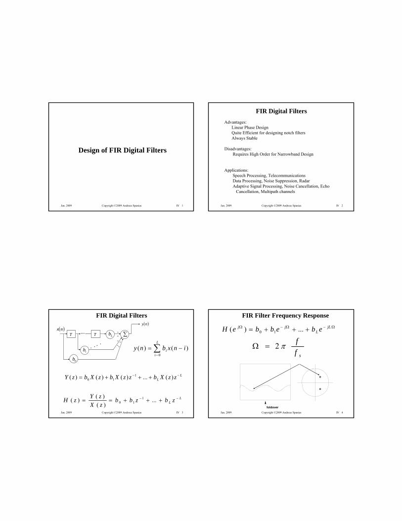
Design of FIR Digital Filters
Jan. 2009 Copyright ©2009 Andreas Spanias IV- 2
FIR Digital Filters
Advantages:Linear Phase DesignQuite Efficient for designing notch filtersAlways Stable
Disadvantages:Requires High Order for Narrowband Design
Applications:Speech Processing, TelecommunicationsData Processing, Noise Suppression, RadarAdaptive Signal Processing, Noise Cancellation, Echo
Cancellation, Multipath channels
Jan. 2009 Copyright ©2009 Andreas Spanias IV- 3
FIR Digital Filters
L
ii inxbny
0
)()(
ny nx
T T
0b
Lb...
.....
1b
.
LL zzXbzzXbzXbzY )(...)()()( 1
10
LL zbzbb
zX
zYzH ...
)(
)()( 1
10
Jan. 2009 Copyright ©2009 Andreas Spanias IV- 4
FIR Filter Frequency Response
jLL
jj ebebbeH ...)( 10
sf
f2
o
o
foldover

Jan. 2009 Copyright ©2009 Andreas Spanias IV- 5
LINEAR PHASE DESIGN
Linear Phase (constant time delay) FIR filter design is important in pulse transmission applications where pulse dispersion must be avoided. The frequency response function of the FIR filter iswritten as:
jLL
jjj ebebebbeH ...)( 2210
where
))(arg()(,)()( jj eHeHM
)()()( eMeH j
Jan. 2009 Copyright ©2009 Andreas Spanias IV- 6
GROUP DELAY
The time delay or group delay of a filter is defined as
d
d )(
therefore if is a linear function of then is aconstant.
is given in terms of samples
Jan. 2009 Copyright ©2009 Andreas Spanias IV- 7
LINEAR PHASE AND IMPULSE RESPONSE SYMMETRIES
It can be shown that linear phase is achieved if
)()( nLhnh
where h(n) is the impulse response of the filter. For L = odd
2
1
0
)( ))(()(
L
n
nLn zznhzH
2
1
0
2
2cos)(2)(
L
n
Ljj n
LnheeH
Jan. 2009 Copyright ©2009 Andreas Spanias IV- 8
SYMMETRIC AND ANTI-SYMMETRIC LINEAR PHASE FILTERS
Two Anti-symmetries for L=even or L=odd for
)()( nLhnh
)()( nLhnh
Two Symmetries for L=even or L=odd for

Jan. 2009 Copyright ©2009 Andreas Spanias IV- 9
EXAMPLES OF SYMMETRIES
nh4L
0
nh
0
nh
0
nh
0
4L
3L
3L
o
Jan. 2009 Copyright ©2009 Andreas Spanias IV- 10
EXAMPLES OF PHASE AND SYMMETRY IN h(n)
Normalized frequency (Nyquist == 1)0 0.1 0.2 0.3 0.4 0.5 0.6 0.7 0.8 0.9 1
-200
-150
-100
-50
0
50
Pha
se (de
gree
s)
0 0.1 0.2 0.3 0.4 0.5 0.6 0.7 0.8 0.9 1-200
-100
0
100
Normalized frequency (Nyquist == 1)
Pha
se(d
egre
es)
0
4L
0
4L
o
Jan. 2009 Copyright ©2009 Andreas Spanias IV- 11
Symmetries and Linear Phase Simulated with J-DSP
Jan. 2009 Copyright ©2009 Andreas Spanias IV- 12
Fourier Series Design Example
For the ideal low pass filter the impulse response sequence is an infinite length sampled sinc function. Lets say the sampling frequency is 8 KHz and we wish to have a cutoff frequency at2 KHz. This results in
28000
200022
s
cc f
f
That is
zHd
2
2

Jan. 2009 Copyright ©2009 Andreas Spanias IV- 13
Fourier Series Design Example (Cont.)
The ideal impulse response hd(n) is given by
,...2,1,0,2
sinc2
1)(
n
nnh d
For an FIR filter of 11 coefficients
,...0,0,
5
1,0,
3
1,0,
1,
2
1,
1,0,
3
1,0,
5
1,0,0...)(
nh
This impulse response is not causal, however a shift operator with 5 delays (z-5) will convert it into a causal DF.
Jan. 2009 Copyright ©2009 Andreas Spanias IV- 14
REALIZATION
. .
5/1 3/1 /1 21 /
...
.1z 1z 1z 1z 1z
1z 1z 1z 1z 1z
ny
nx
Jan. 2009 Copyright ©2009 Andreas Spanias IV- 15
Fourier Series Design Example (Cont.)
5
1,
3
1,
1,
2
1,
1,
3
1,
5
110865420 bbbbbbb
0 0.1 0.2 0.3 0.4 0.5 0.6 0.7 0.8 0.9 1-600
-400
-200
0
Norm alized frequency (Nyquis t == 1)
Ph
as
e (
de
gre
es
)
0 0.1 0.2 0.3 0.4 0.5 0.6 0.7 0.8 0.9 1-80
-60
-40
-20
0
20
Norm alized frequency (Nyquis t == 1)
Ma
gn
itu
de
Re
sp
on
se
(d
B)
Jan. 2009 Copyright ©2009 Andreas Spanias IV- 16
Fourier Series Design Example L=32
32,....1,0,2
)16(sinc
2
1
nn
bn
0 0.1 0.2 0.3 0.4 0.5 0.6 0.7 0.8 0.9 1-2000
-1500
-1000
-500
0
Norm alized frequency (Nyquis t == 1)
Ph
as
e (
de
gre
es
)
0 0.1 0.2 0.3 0.4 0.5 0.6 0.7 0.8 0.9 1-80
-60
-40
-20
0
20
Norm alized frequency (Nyquis t == 1)
Ma
gn
itu
de
Re
sp
on
se
(d
B)

Jan. 2009 Copyright ©2009 Andreas Spanias IV- 17
Fourier Series Design Example L=64
64,....,1,0,2
)32(sinc
2
1
nn
bn
0 0.1 0.2 0.3 0.4 0.5 0.6 0.7 0.8 0.9 1-3000
-2000
-1000
0
Normalized frequency (Nyquis t == 1)
Ph
as
e (
de
gre
es
)
0 0.1 0.2 0.3 0.4 0.5 0.6 0.7 0.8 0.9 1-100
-50
0
50
Normalized frequency (Nyquis t == 1)
Ma
gn
itu
de
Re
sp
on
se
(d
B)
Jan. 2009 Copyright ©2009 Andreas Spanias IV- 18
Truncating with Hamming Window L=64
Hamming(L)sinc xn
bn
2
)32(
2
1
0 0 .1 0 .2 0 .3 0 .4 0 .5 0 .6 0 .7 0 .8 0 .9 1-4 00 0
-3 00 0
-2 00 0
-1 00 0
0
N o rm a liz ed freq ue nc y (N y qu is t = = 1 )
Ph
as
e (
de
gre
es
)
0 0 .1 0 .2 0 .3 0 .4 0 .5 0 .6 0 .7 0 .8 0 .9 1-15 0
-10 0
-5 0
0
5 0
N o rm a liz ed freq ue nc y (N y qu is t = = 1 )
Ma
gn
itu
de
Re
sp
on
se
(d
B)
Jan. 2009 Copyright ©2009 Andreas Spanias IV- 19
F.S. Design; Rectangular vs Hamming Window - L=64
0 0.1 0.2 0.3 0.4 0.5 0.6 0.7 0.8 0.9 1-150
-100
-50
0
50
Normalized frequency (Nyquist == 1)
Mag
nitu
de R
espo
nse
(dB
)
0 0.1 0.2 0.3 0.4 0.5 0.6 0.7 0.8 0.9 1-100
-50
0
50
Normalized frequency (Nyquist == 1)
Mag
nitu
de R
espo
nse
(dB
)
Hamming
Rectangular
~45 dB
~13 dB
Jan. 2009 Copyright ©2009 Andreas Spanias IV- 20
Truncating in time- frequency convolution and F.S. design
•The main-lobe width determines transition characteristics
•The sidelobe level determines rejection characteristics
Ideal LPFNarrow mainlobe=Narrower transition
Wide mainlobe =Wide transition

Jan. 2009 Copyright ©2009 Andreas Spanias IV- 21
Truncating with Short/Long Windows and F.S. design
Wide mainlobe Wide transition
Narrow mainlobe Narrow transition
Ω
Ω
|H(ejΩ)|
|H(ejΩ)|
HLPF(ejΩ)*W(ejΩ)
HLPF(ejΩ)*W(ejΩ)
Wide mainlobe Wide transition
Narrow mainlobe Narrow transition
Ω
Ω
|H(ejΩ)|
|H(ejΩ)|
HLPF(ejΩ)*W(ejΩ)
HLPF(ejΩ)*W(ejΩ)
Wide mainlobe Wide transition
Narrow mainlobe Narrow transition
Ω
Ω
|H(ejΩ)|
|H(ejΩ)|
HLPF(ejΩ)*W(ejΩ)
HLPF(ejΩ)*W(ejΩ)
Jan. 2009 Copyright ©2009 Andreas Spanias IV- 22
Notes On Fourier Series Design
•The design performed in the previous example involved truncationof an ideal symmetric impulse response.A symmetric impulse response produces a linear phase design.
•Truncation involves the use of a window function which is multiplied with the impulse response. Multiplication in the time domain maps into frequency domain convolution and the spectralcharacteristics of the window function affect the design.
•The main-lobe width determines transition characteristics
•The sidelobe level determines rejection characteristics
Jan. 2009 Copyright ©2009 Andreas Spanias IV- 23
DEFINING DESIGN SPECIFICATIONS
2fH
dp1
1dp1
dsLPF Ideal
ffp fs
Passband band Transition Stopband
Regions Tolerance
fc
Jan. 2009 Copyright ©2009 Andreas Spanias IV- 24
DESIGN USING THE KAISER WINDOW
The Kaiser window is parametric and its bandwidth as well as its sidelobeenergy can be designed. Mainlobe bandwidth controls the transition characteristics and sidelobe energy affects the ripple characteristics.
10,)(
1
)(0
2/12
0
LnI
nI
nw
= L/2 ; associated with the order of the filter
is a design parameter that controls the shape of the window
I0(.) is a zeroth order modified Bessel function of the first kind

Jan. 2009 Copyright ©2009 Andreas Spanias IV- 25
DESIGN USING THE KAISER WINDOW (Cont.)
1
2
0 2!
11)(
k
kx
kxI
25 terms from the Bessel function are sufficient
Jan. 2009 Copyright ©2009 Andreas Spanias IV- 26
EXAMPLES OF KAISER WINDOW
0 20 40 60 80 100 120 1400
0.1
0.2
0.3
0.4
0.5
0.6
0.7
0.8
0.9
1
0
5
Jan. 2009 Copyright ©2009 Andreas Spanias IV- 27
KAISER WINDOW DESIGN EQUATIONS
Given fp, fs, T and dp, ds determine the FIR filter coefficients.
Tff
A
dpds
ps )(2
log20
),min(
10
The filter order is )2(285.2
8
A
L
21,0
5021),21(07886.0)21(5842.0
50),7.8(1102.04.0
A
AAA
AA
and the kaiser parameter is given by
Jan. 2009 Copyright ©2009 Andreas Spanias IV- 28
DESIGN PROCEDURE
1. Determine the cutoff frequency for the ideal Fourier Seriesmethod.
ff f
c
s p
22. Design the ideal LPF using the Fourier Series.3. Design the Kaiser window4. Shift and truncate the ideal impulse response
LnL
nhnwnh dLPF
0,
2)()(
Note that this procedure can be generalized for the design of BPF, HPF, and BSF.
Jan. 2009 Copyright ©2009 Andreas Spanias IV- 29
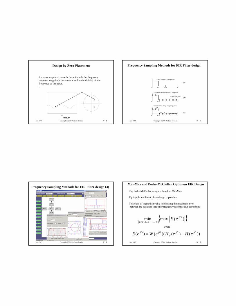
Design by Zero-Placement
As zeros are placed towards the unit circle the frequency response magnitude decreases at and in the vicinity of the frequency of the zeros. .
o
o
foldover
Jan. 2009 Copyright ©2009 Andreas Spanias IV- 30
π/2 π 0 π/4
Ideal frequency response
N=16 samples
π/4 π 0
Sampled ideal frequency response
π/4 π 0
Interpolated frequency response
(a)
(b)
(c)
Frequency Sampling Methods for FIR Filter design
Jan. 2009 Copyright ©2009 Andreas Spanias IV- 31
Frequency Sampling Methods for FIR Filter design (3)
Jan. 2009 Copyright ©2009 Andreas Spanias IV- 32
Min-Max and Parks-McClellan Optimum FIR Design
The Parks-McClellan design is based on Min-Max
Equiripple and linear phase design is possible
This class of methods involve minimizing the maximum errorbetween the designed FIR filter frequency response and a prototype
)(maxmin
,...,1,0),(
j
LiiheE
where
))()()(()( jjd
jj eHeHeWeE

Jan. 2009 Copyright ©2009 Andreas Spanias IV- 33
FIR Filter Design Using MATLAB+
IN THE MATLAB SP TOOLBOX
cremez - Complex and nonlinear phase equiripple FIR filter design.fir1 - Window based FIR filter design - low, high, band, stop, multi.fir2 - Window based FIR filter design - arbitrary response.fircls - Constrained Least Squares filter design - arbitrary response.fircls1 - Constrained Least Squares FIR filter design - low and highpassfirls - FIR filter design - arbitrary response with transition bands.firrcos - Raised cosine FIR filter design.intfilt - Interpolation FIR filter design.kaiserord - Window based filter order selection using Kaiser window.remez - Parks-McClellan optimal FIR filter design.remezord - Parks-McClellan filter order selection.
+ MATLAB is registered trade mark of the MathWorks
Jan. 2009 Copyright ©2009 Andreas Spanias IV- 34
FIR Filter Realizations
Direct Realizations
L
i
ii zbzH
0
)(
•Requires multiply accumulate instructions
...
...
nx
ny
1z
0b1b 2b
1Lb Lb
1z 1z
Jan. 2009 Copyright ©2009 Andreas Spanias IV- 35
FIR Filter Cascade Realizations
Cascade Realizations
q
iiii zbzbbzH
1
22
110 )()(
...1z
1z
1z
1z
10b
11b
12b
20b
21b
22b
nx
•Reduced Effects from Coefficient Quantization and round-off•In Fixed-Point implementation signal scaling must be done carefully at each stage
Jan. 2009 Copyright ©2009 Andreas Spanias IV- 36
Transform-Domain FIR Filter Realizations
A Transform domain realization is possible using the overlapand save and the FFT. This yields computational savings for highorder implementations. Input data is organized in 2N-point blocks and blocks are shifted N points at a time. The data blocks andN zero-padded coefficients are transformed and multiplied and theresults is inverse transformed. The last N-points are selected as theresult. The blocks are updated and the process is repeated.
F F T IF F T
x y
-
X k (0 )
X k (1 )
X k (L )
B k (0 )
B k (1 )
B k (L )
Select Last N points
x(n)
y(n)

Jan. 2009 Copyright ©2009 Andreas Spanias IV- 37
Implementing Efficiently Digital Cross-Over Using Subtractive Operations
LPF to tweeter
to wooferLinear Phase LPFWith delay L/2 samples
-+
could also implement delay compensation z –L/2

Jan. 2009 Copyright © 2009 Andreas Spanias V-1
DESIGN OF IIR DIGITAL FILTERS
Jan. 2009 Copyright © 2009 Andreas Spanias V-2
IIR DIGITAL FILTERS
Advantages:Efficient in terms of order
• Poles create narrow-band peaks efficiently• Arbitrarily long impulse responses with few feedback • coefficients
Disadvantages:• Feedback and stability concerns• Sensitive to Finite Word Length Effects• Generally non-Linear Phase
Applications:• Speech Processing, Telecommunications• Data Processing, Noise Suppression, Radar
Jan. 2009 Copyright © 2009 Andreas Spanias V-3
IIR FILTERS
The difference equation is:
M
ii
L
ii inyainxbny
10
)()()(
nx
z1
0b
... ...
...
.......
- --
ny
1b
Kb
1a
2a
Ma
z1
z1
z1
z1
1Kb
Jan. 2009 Copyright © 2009 Andreas Spanias V-4
IIR FILTERS (Cont.)
The frequency-response function :
The transfer function:
MM
LL
zaza
zbzbb
zX
zYzH
...1
...
)(
)()(
11
110
jM
Mj
jLL
jj
eaea
ebebbeH
...1
...)(
1
10

Jan. 2009 Copyright © 2009 Andreas Spanias V-5
IIR Filter Design by Analog Filter Approximation
The idea is to use many of the successful analog filter designs to design digital filters
This can be done by either:
• by sampling the analog impulse response (impulse invariance)and then determining a digital transfer function
or
• by transforming directly the analog transfer function to a digital filter transfer function using the bilinear transformation
Jan. 2009 Copyright © 2009 Andreas Spanias V-6
IIR Filter Design by Analog Filter Approxination
The impulse invariance method suffers from aliasing and israrely used
The bilinear transformation does not suffer from aliasing and isby more popular than the impulse invariance method.The frequency relationship from the s-plane to the z-plane is non-linear, and one needs to compensate by pre-processing the critical frequencies such that after the transformation the desired response is realized. Stability is maintained in this transformation since the left-half s-plane maps onto the interior of the unit circle.
Jan. 2009 Copyright © 2009 Andreas Spanias V-7
Impulse Invariance
1 1( ) ( ) and ( )
1
t
RCa ah t e u t H j
RC j RC
( ) ( )nT
RCTh n e u n
RC
x(t)
R
C
y(t)i
( / ) 1
( / )( )
1 T RC
T RCH z
e z
ny
1z
8.0
nx
2.0
Jan. 2009 Copyright © 2009 Andreas Spanias V-8
Impulse Invariance (2)
1 2
1 1 1( ) .....a
M
H ss p s p s p
1 21 1 1( ) .....
1 1 1 Mp T p T p T
T T TH z
e z e z e z

Jan. 2009 Copyright © 2009 Andreas Spanias V-9
The Bilinear Transformation
zs
s
1
1planeS planez
Im Im
Re Re
)1
1()(
z
zsHzH
TransformBilinear
Jan. 2009 Copyright © 2009 Andreas Spanias V-10
The Bilinear Transformation (Cont.)
The bilinear transformation compresses the frequency axis
,,
The non-linear frequency transformation (frequency warping function) is given by
2tan
-3 -2 -1 0 1 2 3-15
-10
-5
0
5
10
15
Jan. 2009 Copyright © 2009 Andreas Spanias V-11
Procedure for Analog Filter Approximation
1. Consider Critical Frequencies
2. Pre-warp critical frequencies
3. Analog Filter Design
4. Bilinear Transformation
5. Realization
Jan. 2009 Copyright © 2009 Andreas Spanias V-12
Applying the Bilinear Transformation
ω
Prewarping
Design
bilineartransformation
specification
ω

Jan. 2009 Copyright © 2009 Andreas Spanias V-13
EXAMPLE: TRANSFORMING AN RC CIRCUIT TO A DF
x(t)
R
Ci(t)
ssH
1
1)(
Apply pre-warpingSay we have the following DF specs:
1)4
tan()2
tan(
c
c
Step 3: Design the analog filter.In this case the analog filter function is a first order LPF similar to an RC circuit
2/cStep 1: Step 2:
RCjH
1
1)(
Suppose we want a first-order (R-C LPF) appoximation
Jan. 2009 Copyright © 2009 Andreas Spanias V-14
TRANSFORMING AN RC CIRCUIT TO A DF (2)
15.05.0
11
1
1)
1
1()(
z
zzz
zsHzH
Step 4: Apply the Bilinear Transform
Step 5: Realization
1z
5.0 nx
5.0
ny
Jan. 2009 Copyright © 2009 Andreas Spanias V-15
TRANSFORMING AN RC CIRCUIT TO A DF (3)
jj eeH 5.05.0)(Frequency Response
0 0.1 0.2 0.3 0.4 0.5 0.6 0.7 0.8 0.9 1-100
-80
-60
-40
-20
0
Norm alized frequency (Nyquist == 1)
Ph
as
e (
de
gre
es
)
0 0.1 0.2 0.3 0.4 0.5 0.6 0.7 0.8 0.9 1-60
-40
-20
0
20
Norm alized frequency (Nyquist == 1)
Ma
gn
itu
de
Re
sp
on
se
(d
B)
-1 -0.5 0 0.5 1
-1
-0.5
0
0.5
1
Real part
Ima
gin
ary
pa
rt
0
Notice that there is no aliasing effect with the bilinear transformation.Although in this simple R-C example the resultant digital filter is FIR, more complex analog filters will yield IIR digital filters. Jan. 2009 Copyright © 2009 Andreas Spanias V-16
Analog Filter Designs
•Butterworth - Maximally flat in passband
•Chebyshev I - Equiripple in passband
•Chebyshev II - Equiripple in stopband
•Elliptic - Equiripple in passband and stopband

Jan. 2009 Copyright © 2009 Andreas Spanias V-17
Butterworth Filter Design
• Maximally Flat in the Passband and Stopband
M
C
H2
2
)(1
1|)(|
Jan. 2009 Copyright © 2009 Andreas Spanias V-18
Butterworth Max. Flat in Passband and Stopband
Butterworth frequency response - transition is steeper as order increase
0 20 40 60 80 100 120 1400
0.1
0.2
0.3
0.4
0.5
0.6
0.7
0.8
0.9
1
frequency)
mag
nitu
de
Jan. 2009 Copyright © 2009 Andreas Spanias V-19
Butterworth Transfer Function
M
Cjs
sHsH2)(1
1)()(
12,...,1,0
)1(
1)(
2
)12(2/1
2
Mk
ejs
j
s
M
Mkj
CCM
k
M
C
note that roots can not fall on imaginary axis
Poles on a circle of radius c
Jan. 2009 Copyright © 2009 Andreas Spanias V-20
Design Example - Butterworth
• A Butterworth filter is designed by finding the poles of H(s)H(-s)
• The poles fall on a circle with radius c
• The poles falling on the left hand s-plane (stable poles) are chosen to form H(s)
• H(s) is transformed to H(z)

Jan. 2009 Copyright © 2009 Andreas Spanias V-21
Examples of IIR Filter Design Using MATLAB
FUNCTIONS IN THE SP TOOLBOX
IIR digital filter design.butter - Butterworth filter design.cheby1 - Chebyshev type I filter design.cheby2 - Chebyshev type II filter design.ellip - Elliptic filter design.maxflat - Generalized Butterworth lowpass filter design.yulewalk - Yule-Walker filter design.
IIR filter order selection.buttord - Butterworth filter order selection.cheb1ord - Chebyshev type I filter order selection.cheb2ord - Chebyshev type II filter order selection.ellipord - Elliptic filter order selection.
Jan. 2009 Copyright © 2009 Andreas Spanias V-22
Butterworth Design in MATLAB
• % Design an IIR Butterworth filter
• clear
• N=256; %for the computation of N discrete frequencies
• Wp=0.4; %passband edge
• Ws=0.6; %stopband edge
• Rp=1; % max dB deviation in passband
• Rs=40; %min dB rejection in stopband
• [M,Wn]=buttord(Wp,Ws,Rp,Rs);
• [b,a]=butter(M,Wn);
• theta=[(2*pi/N).*[0:(N/2)-2]]; % precompute the set of discrete frequencies up to fs/2
• H=freqz(b,a,theta); % compute the frequency response
• plot(angle(H))
• pause
• H=(20*log10(abs(H))); % plot the magnitude of the frequency response
• plot(H)
• title('frequency response')
• xlabel('discrete frequency index (N is the sampling freq.)')
• ylabel('magnitude (dB)')
Jan. 2009 Copyright © 2009 Andreas Spanias V-23
Butterworth Design in MATLAB (2)
• Wp=0.4; %passband edge
• Ws=0.6; %stopband edge
• Rp=1; % max dB deviation in passband
• Rs=40; %min dB rejection in stopband
• b = 0.0021 0.0186 0.0745 0.1739 0.2609 0.2609 0.1739
• 0.0745 0.0186 0.0021
• a = 1.0000 -1.0893 1.6925 -1.0804 0.7329 -0.2722 0.0916
• -0.0174 0.0024 -0.0001
Jan. 2009 Copyright © 2009 Andreas Spanias V-24
Butterworth Design in MATLAB (3)
0 2 0 4 0 6 0 8 0 1 0 0 1 2 0 1 4 00
0 . 2
0 . 4
0 . 6
0 . 8
1
1 . 2
1 . 4fre q u e n c y re s p o n s e
d is c re t e fre q u e n c y in d e x (N i s t h e s a m p lin g fr e q . )
ma
gn
itu
de
-1 -0.5 0 0.5 1
-1
-0.5
0
0.5
1
Real part
Ima
gin
ary
pa
rt

Jan. 2009 Copyright © 2009 Andreas Spanias V-25
MATLAB Chebyshev II Design Example
% Design an IIR Chebyshev II filter - Ex 2.20
clearN=256; %for the computation of N discrete frequencies
Wp=0.4; passband edgeWs=0.5; stopband edgeRp=1; ripple in passband (dB)Rs=60; rejection (dB)
[M,Wn] = cheb2ord(Wp,Ws, Rp, Rs); % determine order
[b,a] = cheby2(M,58,Wn); %determine coefficientssize(a)size(b)
% use routines to plot frequency response
Chebyshev I - Equiripple in passbandChebyshev II - Equiripple in stopband
Jan. 2009 Copyright © 2009 Andreas Spanias V-26
IIR Chebyshev II Example
b = 0.0274 0.1065 0.2290 0.3252 0.3252 0.2290 0.1065
.0274
a =1.0000 -0.7484 1.2644 -0.4555 0.3427 -0.0454 0.0186
-0.0002
0 20 40 60 80 100 120 140-100
-90
-80
-70
-60
-50
-40
-30
-20
-10
0frequency response
dis crete frequency index (N is the sam pling freq.)
ma
gn
itu
de
(d
B)
-1 -0.5 0 0.5 1
-1
-0.5
0
0.5
1
Real part
Ima
gin
ary
pa
rt
Jan. 2009 Copyright © 2009 Andreas Spanias V-27
MATLAB Elliptic Design Example
% Design an IIR Elliptic filter clearN=256; %for the computation of N discrete frequencies
Wp=0.4; %passband edgeWs=0.6; %stopband edgeRp=2; % max dB deviation in passbandRs=60; %min dB rejection in stopband[M,Wn] = ellipord(Wp,Ws,Rp,Rs);[b,a] = ellip(M,Rp,Rs,Wn); %design filtersize(a)size(b)
theta=[(2*pi/N).*[0:(N/2)-2]]; % precompute the set of discrete frequencies up to fs/2H=freqz(b,a,theta); % compute the frequency responseplot(angle(H))pauseH=(20*log10(abs(H))); % plot the magnitude of the frequency responseplot(H)title('frequency response')xlabel('discrete frequency index (N is the sampling freq.)')ylabel('magnitude (dB)')pausezplane(b,a) ;% z plane plot
Jan. 2009 Copyright © 2009 Andreas Spanias V-28
IIR Elliptic
-1 -0.5 0 0.5 1
-1
-0.5
0
0.5
1
Real part
Ima
gin
ary
pa
rt
0 20 40 60 80 100 120 140-4
-3
-2
-1
0
1
2
3
4
0 20 40 60 80 100 120 140-90
-80
-70
-60
-50
-40
-30
-20
-10
0
frequency response
discrete frequency index (N is the sampling freq.)
ma
gn
itu
de
(d
B)
b = 0.0181 0.0431 0.0675 0.0675 0.0431 0.0181
a = 1.0000 -2.3214 3.3196 -2.8409 1.5154 -0.4151

Jan. 2009 Copyright © 2009 Andreas Spanias V-29
Introduction to Special types of Digital Filters
• Shelving Filter
• Peaking Filter
• Graphic Equalizer
Jan. 2009 Copyright © 2009 Andreas Spanias V-30
Shelving Filters
Shelving filters realize tone controls in audio systems. The frequency response of a low-pass (bass) and high-pass (treble) shelving filter is shown below.
Frequency response of a low-pass and high-pass shelving filter.
Jan. 2009 Copyright © 2009 Andreas Spanias V-31
Tone Control Block in J-DSPThe low frequencies are affected by bass adjustments with the audio signal processed through low-pass shelving filters. The high frequencies are affected by treble adjustments with the audio signal processed through high-pass shelving filters. A J-DSP simulation using the Tone Control . Figure J-DSP simulation using the tone control block.
Jan. 2009 Copyright © 2009 Andreas Spanias V-32
Peaking Filter Block in J-DSP
A J- DSP simulation using the Peaking Filter block is shown below
Figure 9: J-DSP simulation using the peaking filter block.

Jan. 2009 Copyright © 2009 Andreas Spanias V-33
Graphic Equalizer• A graphic equalizer uses a cascade of peaking filters • It alters the frequency response of each band by varying the
corresponding peaking filter’s gain.
PeakingFilter#1
PeakingFilter#2
PeakingFilter#N-1
PeakingFilter#N
+ + +
Input
Output
…
…
…
A diagram of a graphic equalizer with N bands of control. Jan. 2009 Copyright © 2009 Andreas Spanias V-34
Graphic Equalizer Block in J-DSP
A J- DSP simulation using the Graphic Equalizer block is shown below. The sliders are a graphic representation of the frequency response applied to the input audio signal, hence the name “graphic” equalizer.
-DSP simulation using the graphic equalizer block.
Jan. 2009 Copyright © 2009 Andreas Spanias V-35
FIR vs IIR Digital Filters
FIR IIRAlways stableTransversalAll-zero modelMoving Average(MA) model
Inefficient for spectral peaks
Efficient for spectral notches
Not always stableRecursiveAll-pole or Pole-zero modelAutoregressive(AR) or
Autoregressive MovingAverage (ARMA) model
Efficient for spectral peaks (all-pole, pole-zero)
All pole inefficient for spectralnotches
Jan. 2009 Copyright © 2009 Andreas Spanias V-36
FIR IIR
FIR vs IIR Digital Filters (Cont.)
Pole-zero efficient for both notches and peaks
Generally requires lowerorder design
More sensitive to finite wordlength implementation
Generally non-linear phase
Requires high order design
Less sensitive to finite wordlength implementation
Linear phase design

Jan. 2009 Copyright © 2009 Andreas Spanias V-37
Digital Audio Filters (1)
The echo effect is obtained by mixing the input signal with its delayed version.
The proportion of the delayed signal to the "clean" original signal determines how obvious the echo is, and the delay signifies the echo period.
Echo Effects
• R = the number of echo delay in samples.
• In order to have a distinguishable echo, R
should be relatively large.
• b is the attenuation constant (|b| < 1).
y(n)= x(n) + b . x(n-R)
Echo
Jan. 2009 Copyright © 2009 Andreas Spanias V-38
Digital Audio Filters (2)
Reverberation is obtained bymixing the input signal with the delayed versions of its feedback.
The effect of the feedback results in multiple echoes.
Reverberation Effects
Reverb
• R = feedback delay in samples.
• b is the attenuation constant (|b| < 1).
y(n) = x(n) + b . y(n-R)
Jan. 2009 Copyright © 2009 Andreas Spanias V-39
Other Methods for Digital Filtering
Median Filters
The median operation ranks the samples in the memory of the filter and picks the sample that falls in the middle of the rank and assigns it to the output y(n)
Used for impulsive noise. One application reported is scratch noise removal in vinyl record restoration
)()(,...,2,1,0
inxny medianLi
Jan. 2009 Copyright © 2009 Andreas Spanias V-40
2-D Filters for Image Applications
• FIR 2-D filter
• IIR realizations also possible
• Theory very similar to 1-D and described in multidimensional signal processing books
1 2 1 2 1 20 0
( , ) ( , ) ( , )L M
l m
y n n h n n x n l n m

Jan. 2009 Copyright © 2009 Andreas Spanias V-41
Implementation of 2D Filters
High-pass filtering of a natural image Low-pass filtering of a natural
image
LPFLPF
HPFHPF
1
Jan. 2009 Copyright (c) 2009 Andreas Spanias VII-1
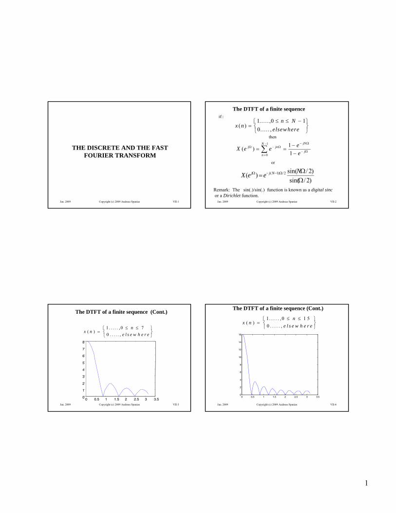
THE DISCRETE AND THE FAST FOURIER TRANSFORM
Jan. 2009 Copyright (c) 2009 Andreas Spanias VII-2
The DTFT of a finite sequence
then
j
jNN
n
jnj
e
eeeX
1
1)(
1
0
or
)2/sin(
)2/sin()( 2/)1(
NeeX Njj
x nn N
elsew here( )
. . . . . ,
. . . . . ,
1 0 1
0
if::
Remark: The sin(.)/sin(.) function is known as a digital sincor a Dirichlet function.
Jan. 2009 Copyright (c) 2009 Andreas Spanias VII-3
The DTFT of a finite sequence (Cont.)
x nn
e l s e w h e r e( )
. . . . . ,
. . . . . ,
1 0 7
0
0 0.5 1 1.5 2 2.5 3 3.50
1
2
3
4
5
6
7
8
Jan. 2009 Copyright (c) 2009 Andreas Spanias VII-4
The DTFT of a finite sequence (Cont.)
x nn
e l s e w h e r e( )
. . . . . ,
. . . . . ,
1 0 1 5
0
0 0.5 1 1.5 2 2.5 3 3.50
2
4
6
8
10
12
14
16

2
Jan. 2009 Copyright (c) 2009 Andreas Spanias VII-5
The Discrete Fourier Transform (DFT)
12 /
0
( ) ( )N
j kn N
n
X k x n e
and k = 0, 1, . . . , N-1
The inverse Discrete Fourier Transform (IDFT) of the sequence x(n)
1
0
/2)(1
)(N
k
NknjekXN
nx and n = 0, 1, …, N-1
The DFT transform pair is denoted by
x n X k( ) ( )Jan. 2009 Copyright (c) 2009 Andreas Spanias VII-6
The DFT Matrix
The DFT and the IDFT may be expressed in terms of matrices, i.e.,
where k j k Ne 2 /
1-Nx
.
.
2x
1x
0x
... 1
. ... . . .
. ... . . .
... 1
... 1
1 ... 1 1 1
NX
.
.
X
X
X
-1N--1N2--1N-
-1N2-4-2-
-1N-2--1
21
2
1
0
a more compact form xFX
HFN
F11
and
XFx 1and
Jan. 2009 Copyright (c) 2009 Andreas Spanias VII-7
The DFT Matrix (2)
1 1
1 -1
F
1 1 1
1 0.5 0.866 0.5 0.866
1 0.5 0.866 0.5 0.866
j j
j j
F
1 1 1 1
1 1
1 1 1 1
1 1
j j
j j
F
N=2, N=4, and N=8
Jan. 2009 Copyright (c) 2009 Andreas Spanias VII-8
Selected Properties of the DFT
Linearity:
Shifting:
Circular Convolution:
Freq. Circular Convolution:
Parseval’s Theorem:
x n y n X k Y k( ) ( ) ( ) ( )
x n m N e X kj km N( ) mod ( )/ 2
x nN
X kn
N
k
N
( ) ( )2
0
12
0
11
x n h n X k H k( ) ( ) ( ) ( )
where N
N
m
mhnhnx mod
1
0
m-n x
x n w nN
X k W k( ) ( ) ( ) ( ) 1

3
Jan. 2009 Copyright (c) 2009 Andreas Spanias VII-9
Frequency resolution of the DFT
The frequency resolution of the N-point DFT is
ff
Nrs
•The DFT can resolve exactly only the frequencies fallingexactly at: k fs/N. There is spectral leakage for componentsfalling between the DFT bins
•Typically we use an FFT that is as large as we can afford
•Zero-padding is often use to provide more resolution in thefrequency components
•Zero padding is often combined with tapered windowsJan. 2009 Copyright (c) 2009 Andreas Spanias VII-10
Spectral Estimates over Finite-time Data windows
Frequency domain representations are appropriately defined by theFourier Transform integrals over an infinite time span.
The DFT, however, estimates the spectrum over finite time
The DFT essentially applies a window to truncate the data.
The simplest data window is the rectangular (boxcar).
Truncation in time is convolution in frequency
The frequency domain characteristics of the data window, namely its bandwidth and sidelobes, affect the DFT spectral estimate.
Jan. 2009 Copyright (c) 2009 Andreas Spanias VII-11
WINDOWS
The spectral characteristics of the window affect the spectral estimates. The
rectangular window has the narrowest mainlobe width but the wordt sidelobes.
Tapered windows have wider mainlobe width but better behaved bandwidth.
- 57 dB12 π /NBlackman
- 31 dB8 π /NHanning
- 41 dB8 π /NHamming
- 25 dB8 π /NTriangular
-13 dB4π/(N+1)Rectangular
Sidelobe
Level
Mainlobewidth
N-point
Window
Jan. 2009 Copyright (c) 2009 Andreas Spanias VII-12
FFTs of Sinusoidal Signals (1)
256-point FFT of a 500 Hz sinusoid (fs=8 kHz). Notice that this sinusoid is resolved exactly
0 50 100 150 200 250 300-350
-300
-250
-200
-150
-100
-50
0
50FFT
disc rete frequency index (N is the sam pling freq.)
ma
gn
itu
de
(d
B)

4
Jan. 2009 Copyright (c) 2009 Andreas Spanias VII-13
FFTs of Sinusoidal Signals (2)
256-point FFT of a 510 Hz sinusoid (fs=8 kHz). Notice that this sinusoid is NOT resolved exactly
0 50 100 150 200 250 300-5
0
5
10
15
20
25
30
35
40
45FFT
discrete frequency index (N is the s ampling freq.)
ma
gn
itu
de
(d
B)
Jan. 2009 Copyright (c) 2009 Andreas Spanias VII-14
Zero-padded FFTs of Sinusoidal Signals (2)
16-point FFT of a 16-point 590 Hz sinusoid (fs=8 kHz).Vs
256-point FFT of a 16-point 590 Hz sinusoid (fs=8 kHz).Notice that although this sinusoid is NOT resolved exactly the frequency of the peak in the zero-padded case is closer to actual
0 2 4 6 8 10 12 14 16-10
-5
0
5
10
15
20FFT
discrete frequency index (N is the sam pling freq.)
ma
gn
itu
de
(d
B)
0 50 100 150 200 250 300-10
-5
0
5
10
15
20FFT
discrete frequency index (N is the sam pling freq.)
ma
gn
itu
de
(d
B)
Jan. 2009 Copyright (c) 2009 Andreas Spanias VII-15
Windowed FFTs on Sinusoids
0 50 100 150 200 250 300-10
-5
0
5
10
15
20boxc ar windowed FFT
dis crete frequenc y index (N is the sam pling freq.)
ma
gn
itu
de
(d
B)
boxcar. hamming
hanning
0 50 100 150 200 250 300-80
-70
-60
-50
-40
-30
-20
-10
0
10
20hanning windowed FFT
disc rete frequency index (N is the sam pling freq.)
ma
gn
itu
de
(d
B)
0 50 100 150 200 250 300-50
-40
-30
-20
-10
0
10
20hamm ing windowed FFT
discrete frequency index (N is the sampling freq.)
ma
gn
itu
de
(d
B)
Jan. 2009 Copyright (c) 2009 Andreas Spanias VII-16
Window Comparison with Closely Spaced Periodicities
boxcar. hamming
high resolution ---->
0 100 200 300 400 500 6000
5
10
15
20
25
30
35boxcar windowed 512-point FFT of two 32 point s inusoids
disc rete frequency index (N is the sam pling freq.)
ma
gn
itu
de
(d
B)
0 100 200 300 400 500 600-20
-15
-10
-5
0
5
10
15
20
25
30
Hamm ing windowed 512-point FFT of two 32 point s inusoids
dis crete frequency index (N is the sam pling freq.)
ma
gn
itu
de
(d
B)
0 1000 2000 3000 4000 5000 6000 7000 8000 9000-30
-20
-10
0
10
20
30
40
50
60
High Resolution"
dis c rete frequenc y index (N is the sam pling freq.)
ma
gn
itu
de
(d
B)

5
Jan. 2009 Copyright (c) 2009 Andreas Spanias VII-17
Window Comparison with Distant Periodicities
boxcar. hamming
High Resolution
0 100 200 300 400 500 600-30
-20
-10
0
10
20
30
40
50
Ham ming windowed 512-point FFT of two 8192 point s inusoids
discrete frequency index (N is the sampling freq.)
ma
gn
itu
de
(d
B)
0 100 200 300 400 500 600-10
0
10
20
30
40
50
B oxcar windowed 512-point F FT of two 32-point dis tant s inusoids
disc rete frequency index (N is the sam pling freq.)
ma
gn
itu
de
(d
B)
0 1000 2000 3000 4000 5000 6000 7000 8000 9000-40
-20
0
20
40
60
80
High Resolut ion"
discrete frequency index (N is the sam pling freq.)
ma
gn
itu
de
(d
B)
Jan. 2009 Copyright (c) 2009 Andreas Spanias VII-18
The FFT-DIT Algorithm
The FFT decimates the sequence and performs a DFT by processing results
of smaller size DFTs. This is done by decomposing the N-point DFT to 2-
point DFTs and using “butterfly” operations to obtain the result. For a
Decimation in Time (DIT) FFT algorithm the following steps are taken:
X k x n e j n k N
n
N
( ) ( ) /
2
0
1
By decimating x(n) we can write
X k x n e x n ej nk N
n
Nj n k N
n
N
( ) ( ) ( )/( / )
( ) /( / )
2 2 12 2
0
2 12 2 1
0
2 1
Jan. 2009 Copyright (c) 2009 Andreas Spanias VII-19
The FFT-DIT Algorithm (Cont.)
if we define NnkjnkN eWnxnxnxnx /2
21 )12()()2()(
1)2/(
02/22
1)2/(
02/11 )()()()(
N
n
nkN
N
n
nkN WnxkXWnxkX
and
)()()2/(
12/,...,1,0),()()(
21
21
kXWkXNkX
NkkXWkXkXk
N
kN
Remarks: The N-point DFT is broken down to two N/2-point DFTs. We then write the
N/2-point DFTs as a combination of two N/4-point DFTs and so forth.
Jan. 2009 Copyright (c) 2009 Andreas Spanias VII-20
DFT
intpo4
0x
DFT
intpo4
2x
4x
6x
01X
11X
21X
31X
0X
1X
2X
3X
1x
3x
5x
7x
02X
12X
22X
32X
4X
5X
6X
7X
1
1
1
1
08W1
8W2
8W3
8W
The FFT-DIT Algorithm (Cont.)

6
Jan. 2009 Copyright (c) 2009 Andreas Spanias VII-21
X'(0)
X'(1)
X'(0)
X'(1)
1
1
2
2
X'(0)
X'(1)
X'(0)
X'(1)
3
3
4
4
-1
X (0)
X (1)
X (2)
X (3)
1
1
1
1
X (0)
X (1)
X (2)
X (3)
2
2
2
2
-1
-1
-1
-1
W80
W82
W80
W82
-1
-1
-1
x(0)
x(2)
x(4)
x(6)
x(1)
x(3)
x(5)
x(7)
-1
-1
-1
-1
X(0)
X(1)
X(2)
X(3)
X(4)
X(5)
X(6)
X(7)
W80
W81
W82
W83
The FFT-DIT Algorithm (Cont.)
Jan. 2009 Copyright (c) 2009 Andreas Spanias VII-22
The DFT and the FFT Complexity
The N-point DFT requires N2 multiplications and N2 –1 additions to
compute the discrete frequency spectrum.
The complexity of the DFT is reduced using the FFT to
N/2 log2N multiplications and N log2N additions.
For example if N=4096 the DFT requires 16,777,216
multiplications while the FFT requires 49,152 multiplications.
Jan. 2009 Copyright (c) 2009 Andreas Spanias VII-23
FFT ALGORITHMS
IN FFT DECIMATION-IN-TIME-the frequency-domain (output) indices are in place while the time-domain(input) indices are bit-reversed
IN FFT DECIMATION-IN-FREQUENCY-the time-domain indices are in place while the frequency-domain indices arebit-reversed
VARIANTS OF FFT ALGORITHMS:Low-Complexity "Prunned" FFTs
- For computing fewer frequency bins- when time-domain values are systematically zero (ex: zero padded FFTs)
Radix 4 and Mixed-radix FFTs, Gortzel Algorithm (computes only one frq. bin),Rader, Prime Factor, Winograd, Zoom FFTs
Reference: E. Brigham, "The FFT and its Applications," Prentice Hall, NJ 1988Links on FFT: http://www.fftw.org/links.htmlFFT laboratory: http://sepwww.stanford.edu/oldsep/hale/FftLab.html
Jan. 2009 Copyright (c) 2009 Andreas Spanias VII-24
FFT Applications

7
Jan. 2009 Copyright (c) 2009 Andreas Spanias VII-25
FFT AND SPEECH ENHANCEMENT
•If we have speech corrupted by background noise, the spectrum of background noise can be estimated during speech pauses.
•Speech is enhanced in the spectral domain by subtracting the estimated noise spectrum from the noisy speech spectrum
•FFT-based spectral subtraction is used in military applications
•Also used in CDMA cellular IS-127 telephony standard
Jan. 2009 Copyright (c) 2009 Andreas Spanias VII-26
FFT SPEECH ENHANCEMENT IN CDMA
Window/FFTOverlap/add
IFFT
X
S (n)HP
Channel Gain
Computation
Channel Energy
Estimator
Channel SNR Noise
EstimatorEstimator
Channel SNR
Modification
Spectral
Estimator
Voice Metric
Computation
Noise Uodate
Decision
G(k) H(k)
Update Flag
Ech(m) En(m)
v(m)
Etot(m)
Deviation
Jan. 2009 Copyright (c) 2009 Andreas Spanias VII-27
FFT AND SINUSOIDAL TRANSFORM CODING
PHASES
FREQUENCIES
AMPLITUDES
FRAME-TO-FRAME PHASE
UNWRAPPING & INTERPOLATION
FRAME-TO-FRAME LINEAR
INTERPOLATION
SINE WAVE GENERATOR x SUM ALL
SINE WAVES
SYNTHETIC
SPEECH
Implemented by IFFT and overlap&add procedure
FFTSpeech
TAN-1(.)PHASES
FREQUENCIES
AMPLITUDES
Peak Picking
.
ENCODER
DECODER
R. McAulay and T. Quatieri, “Sinsoidal Coding,”Ch. 4, Speech Coding and Synthesis, W.B. Kleijn and K. Paliwal, eds, Elsevier, 1995.
Jan. 2009 Copyright (c) 2009 Andreas Spanias VII-28
Simple FFT Based Compression
DFT Analysis
IDFT Synthesis
Redundancy Removal
Input signal vector x
Output signal vector
x^

8
Jan. 2009 Copyright (c) 2009 Andreas Spanias VII-29
Fast Convolution Using the FFT
• Fast Circular Convolution
b. Fast Linear Convolution
FFTs are often used to compute efficiently convolutions ofvery long sequences. Such convolutions arise in adaptive filtersthat are used in noise and echo cancellation.
Jan. 2009 Copyright (c) 2009 Andreas Spanias VII-30
Fast N-point Circular Convolution
X
FFT
FFT
IFFT
x(n)
h(n)
X(k)
H(k)
Y(k) y(n)
Jan. 2009 Copyright (c) 2009 Andreas Spanias VII-31
Fast N-point Linear Convolutionusing the Overlap/Save
X
2NFFT
2NIFFT
x(n)
h(n)
X(k)
H(k)
Y(k)
y(n)
0
1
0
1
2NFFT
Jan. 2009 Copyright (c) 2009 Andreas Spanias VII-32
J-DSP and Fast Convolution

9
Jan. 2009 Copyright (c) 2009 Andreas Spanias VII-33
Orthogonal Frequency Division Multiplexing (OFDM) and FFTs
)()()(
,,1)()()/2()(
H nnn
NknwnsNkHnz kkk
vsDz