Disaster Risk in a New Keynesian Model - CEPII - Accueil · CEPII Working Paper Disaster Risk in a New Keynesian Model DISASTER RISK IN A NEW KEYNESIAN MODEL Marlène Isoré and Urszula

C E N T R ED ’ É T U D E S P R O S P E C T I V E SE T D ’ I N F O R M A T I O N SI N T E R N A T I O N A L E S

No 2013-12

April

DO

CU

ME

NT

DE

TR

AV

AI

L

Disaster Risk in a New Keynesian Model

Marlène Isoré and Urszula Szczerbowicz

CEPII Working Paper Disaster Risk in a New Keynesian Model

TABLE OF CONTENTS

Highlights and Abstract . . . . . . . . . . . . . . . . . . . . . . . . . . . 3Points clefs et résumé. . . . . . . . . . . . . . . . . . . . . . . . . . . . 41. Introduction . . . . . . . . . . . . . . . . . . . . . . . . . . . . . . 52. Model . . . . . . . . . . . . . . . . . . . . . . . . . . . . . . . . 7

2.1. Households . . . . . . . . . . . . . . . . . . . . . . . . . . . . 72.2. Firms . . . . . . . . . . . . . . . . . . . . . . . . . . . . . . . 102.3. Public authority . . . . . . . . . . . . . . . . . . . . . . . . . . . 13

3. Equilibrium . . . . . . . . . . . . . . . . . . . . . . . . . . . . . . 143.1. Market clearing . . . . . . . . . . . . . . . . . . . . . . . . . . . 143.2. Calibration and steady-state analysis . . . . . . . . . . . . . . . . . . 14

4. Impulse responses of the macroeconomic variables . . . . . . . . . . . . . . 164.1. A rise in the probability of disaster . . . . . . . . . . . . . . . . . . . 164.2. Standard shocks. . . . . . . . . . . . . . . . . . . . . . . . . . . 18

5. Further research . . . . . . . . . . . . . . . . . . . . . . . . . . . . 186. Conclusion . . . . . . . . . . . . . . . . . . . . . . . . . . . . . . 19References . . . . . . . . . . . . . . . . . . . . . . . . . . . . . . . . 21Appendix . . . . . . . . . . . . . . . . . . . . . . . . . . . . . . . . 238. Mathematical Appendix . . . . . . . . . . . . . . . . . . . . . . . . . 23

A. Households . . . . . . . . . . . . . . . . . . . . . . . . . . . . 23B. Firms . . . . . . . . . . . . . . . . . . . . . . . . . . . . . . . 23C. Aggregation . . . . . . . . . . . . . . . . . . . . . . . . . . . . 27D. Full set of equilibrium conditions . . . . . . . . . . . . . . . . . . . . 31E. Steady-state . . . . . . . . . . . . . . . . . . . . . . . . . . . . 33

2


DISASTER RISK IN A NEW KEYNESIAN MODEL


HIGHLIGHTS

We incorporate a small and time-varying “disaster risk” in a New Keynesian model.A higher probability of disaster is sufficient to generate a recession without effective occur-rence of the disaster.The dynamic responses of macroeconomic quantities are discussed relatively to a flexibleprice benchmark.

ABSTRACT

This paper incorporates a small and time-varying “disaster risk” à la Gourio (2012) in a New Keynesianmodel. A change in the probability of disaster may affect macroeconomic quantities and asset prices. Inparticular, a higher risk is sufficient to generate a recession without effective occurrence of the disaster.By accounting for monopolistic competition, price stickiness, and a Taylor-type rule, this paper providesa baseline framework of the dynamic interactions between the macroeconomic effects of rare events andnominal rigidity, particularly suitable for further analysis of monetary policy. We also set up our nextresearch agenda aimed at assessing the desirability of several policy measures in case of a variation inthe probability of rare events.

JEL Classification: E17, E20, E32, G12

Keywords: disaster risk, rare events, DSGE models, business cycles.

3


DISASTER RISK IN A NEW KEYNESIAN MODEL


POINTS CLEFS

Nous incorporons un risque faible et variable dans le temps de “désastre” économique dansun modèle néo-keynésien.Un accroissement de la probabilité de désastre s’avère suffisant pour générer une récessionsans occurrence effective de ce désastre.Nous comparons les dynamiques des quantités macroéconomiques ainsi obtenues en présenceet en l’absence de rigidités nominales.

RÉSUMÉ

Ce document introduit dans un modèle néo-keynésien un risque faible et variable dans le temps de "dé-sastre" économique à la Gourio (2012). Une légère variation de la probabilité de désastre affecte lesquantités macroéconomiques et les prix des actifs. En particulier, un accroissement du risque s’avèresuffisant pour générer une récession sans occurrence effective du désastre. En étudiant cet effet dansun cadre néo-keynésien standard, en concurrence monopolistique avec rigidité des prix et en présenced’une règle de politique monétaire, nous fournissons un cadre de référence pour l’étude des interactionsdynamiques entre les effets macroéconomiques des événements rares et les rigidités nominales. Nousproposons enfin un programme de recherche visant à évaluer l’impact de différentes politiques écono-miques, notamment de mesures monétaires non conventionnelles, en cas d’augmentation de la probabilitéde désastre.

Classification JEL : E17, E20, E32, G12

Mots clés : Risque de désastre, événements rares, modèles DSGE, business cycles.

4


DISASTER RISK IN A NEW KEYNESIAN MODEL1

Marlène Isoré∗ and Urszula Szczerbowicz†

1. INTRODUCTION

A recent but growing literature studies how the risk of rare events — sometimes called economic“disasters” — affects the dynamic interactions between macroeconomic quantities and assetprices — risk premia in particular. However, disaster risk is still rarely accounted for in generalequilibrium models, especially in the models used to conduct monetary policy where variationsin the expected returns are generally entirely driven by variations in the risk-free interest rate.Yet understanding the efficiency and the desirability of monetary policy facing — realized orpotential — rare events is of main interest. In order to design an appropriate intervention,studying the effects of a time-varying disaster risk in this class of models is a prerequisite.

Early papers on disaster risk were restricted to endowment economies (Rietz, 1988, Barro, 2006,Gabaix, 2012) such that policy implications could have hardly been derived. Gourio (2012) hasgone a step further by introducing a small and stochastically time-varying risk premium into areal business cycle model. His model has thus provided a tractable way to analyze the feedbackeffects between changes in aggregate risk and the macroeconomic variables, as well as to repro-duce some important empirical facts in terms of asset pricing including the countercyclicalityof the risk premia. In particular, an increase in the probability of disaster leads investment andoutput to fall as capital becomes riskier. Meanwhile precautionary savings lower the yield onrisk-free assets, such that the spread rises in distressed times.

This paper builds on Gourio’s approach and introduces a time-varying risk of disaster in anotherwise standard New Keynesian DSGE model, providing a baseline framework that willallow to evaluate the role of monetary policy facing changes in the probability of rare events.The occurrence of a disaster is associated with the destruction of a share of capital, but theappealing feature of the model is that business cycles are significantly affected by the disasterrisk even when disasters do not effectively arrive. We especially focus on the responses ofmacroeconomic quantities to a sudden rise in the probability of disaster, and get some interestingpreliminary results.

1We thank Pierpaolo Benigno, Julio Carrillo, Benjamin Carton, Rich Clarida, Marco Del Negro, François Gourio,Salvatore Nisticò, Henri Sterdyniak, and Philippe Weil for many discussions from the early stages of this work.All remaining errors are ours.∗MIT Economics, 50 Memorial Drive, Cambridge MA 02142. Email: [email protected]†CEPII, 113 rue de Grenelle, 75007 Paris, France. Email: [email protected]

5


First, we are able to relax one essential assumption in Gourio’s work which consists in imposinga reduction in total factor productivity by exactly the same amount than the capital stock toreplicate the data. We show that the output fall may be large enough by introducing investmentadjustment costs and monopolistic competition in intermediate goods instead. The responseof output is much more important under time-dependent price stickiness, however, since firmsmay be more inclined to adjust their prices when the aggregate risk rises (Caplin and Leahy,1991), we also allow for some state-dependent price adjustment.

Second, we find that consumption falls on impact in case of a rise in disaster risk while Gouriofound the opposite response with a more stylized model. Similarly, we get a drop in wageswhich is not observed in the pure flexible-price but otherwise similar version of the model,that seems more reminiscent of distressed economic times, whether under time-dependent orstate-dependent price stickiness. Finally, we compare the responses of the model to standardmonetary, fiscal, and productivity shocks, with and without the presence of a disaster risk.

This version of the model does not study the feedback effects between these macroeconomicquantities and the impact of disaster risk on asset pricing yet. However, the set-up is such thatwe will be able to do so quite easily by already incorporating a stochastic discount factor fromwhich the term premium will be derived and some features that proved effective in replicat-ing the variations of equity premia, including habit formation.2 Gourio (2012) shows that thepresence of a time-varying disaster risk allows to replicate well the first- and second momentsof asset returns, as well as their correlation with the macroeconomic quantities. This suggeststhat the degree of risk aversion or the amount of risk in the economy has a significant impacton macroeconomic dynamics while Tallarini (2000)’s “observational equivalence” only holdswhen the probability of disaster is constant over time. In our model, solved under certainty-equivalence so far, linear and nonlinear approximations give almost identical results since westudy the responses of macroeconomic quantities to a (small) change in the probability of dis-aster instead of the responses to a (large) disaster shock. Asset pricing in the presence of atime-varying disaster risk would however require the combination of nonlinear methods andaggregate uncertainty.3

The remainder of the paper is as follows. Section 2 develops the model, Section 3 discusseshow the steady state is affected by the presence of a disaster risk and presents the calibration,Section 4 describes the response functions to a shock to the probability of disaster as well as tostandard shocks. Section 5 gives our further research agenda, and Section 6 concludes.

2See Campbell and Cochrane (1999) and Uhlig (2007).3See Bloom (2009) for a model with uncertainty shocks for instance.

6


2. MODEL

2.1. Households

Households consume goods, supply labor, and save through risk-free bonds and capital accu-mulation so as to maximize the expected discounted sum of utility flows given by

E0

∞

∑t=0

βt

((Ct−hCt−1)

1−γ

1− γ−χ

L1+φ

t

1+φ

)(1)

where β is the subjective discount factor, E0 the expectation operator, C and L consumption andlabor flows respectively, h a habit formation parameter, γ the coefficient of relative risk aversionor the inverse of the intertemporal elasticity of substitution, and φ the inverse of the elasticityof work effort with respect to the real wage. Households own the capital stock Kt and lease afraction ut of it to the firms. Thus their budget constraint is

Ct + It +Bt+1

pt≤WtLt +(1+ it−1)

Bt

pt+Rk

t utKt +Πt−Tt (2)

where It is investment, Bt are one-period bonds, wt is the real wage, Πt are profits from firms,and Rk

t is the real rental rate of capital, at time t.

Capital is considered as a risky asset here in the sense that it may be hit by a “disaster”. In Barro(2006) and Gourio (2012)’s spirit, a disaster occurrence may be either a war which physicallydestroys a part of the capital stock, the expropriation of capital holders, a technological revolu-tion that make it worthless, or the loss of intangible capital due to a prolonged recession. Weassume that the disaster destroys a share bk of the capital stock if realized.4 Therefore the lawof capital accumulation is given by

Kt+1 =

(1−δt)Kt +

[1−S

(It

It−1

)]It

(1− xt+1bk) (3)

where δt = δuη

t is the depreciation rate increasing with capital utilization (Burnside and Eichen-

baum, 1996), and S = τ

2

(It

It−1−1)2

is a capital adjustment cost function which verifies the usualproperties (S(0) = 0, S′(0) = 0, and S′′(.) > 0). The disaster is captured by the indicator xt+1which is equal to 1 with probability θt and equal to 0 otherwise. Gourio (2012) argues thatthis probability can be considered as strict rational expectations or more generally account for

4As a disaster lowers the return on capital because investing in capital is riskier one can equally consider ex antethat this is the price or the quantity of capital which is affected by the disaster.

7


time-varying beliefs which may differ from the objective probability.5 We consider that the logof the probability of disaster follows a first-order autoregressive process as

logθt = (1−ρθ ) log θ +ρθ logθt−1 +σθ εθt (4)

and assume that the shocks θt+1 and xt+1 are independent, conditional on θt , in line with theevidence that a disaster occurrence tomorrow is not likely if there is a disaster today (Gourio,2008).

We relax Gourio (2012)’s assumption that total factor productivity is reduced by exactly thesame amount than the capital (bk) in case of a disaster here. This assumption has been made fortwo reasons. First, detrending the capital by the (stochastic) technology level gives a stationaryvariable and reduces the dimension of the state space, so as to obtain analytical results andsimplify the numerical analysis. Second, it delivers an empirically relevant magnitude for therecession. However, the combination of adjustment costs and monopolistic competition allowsus to replicate a large enough fall in output following a rise in disaster risk without havingto maintain this assumption here. Moreover, while Gourio argues that some disasters wereassociated with a fall in TFP (South America since 1945, Russia in 1917), some papers find,on the contrary, that TFP may rise in recessions as the least productive firms are shut down (forinstance Petrosky-Nadeau, 2010).

Maximizing (1) subject to (2), (3), and (4) gives standard first-order conditions for consumption,labor, and the riskfree bonds, respectively as

λt = (Ct−hCt−1)−γ −βhEt(Ct+1−hCt)

−γ (5)

χLφ

t = wtλt (6)

λt = βEtλt+1(1+ it)(1+πt+1)−1 (7)

in which 1+πt+1 ≡ pt+1pt

where π is the (net) inflation rate, whereas the first-order conditionsfor capital and capital utilization are both affected by the disaster probability and the disastersize effect, θtbk, as follows6

µt = βEt

[λt+1Rk

t+1ut+1 +µt+1(1−δuη

t+1)(1−θt+1bk)

](8)

5Building on the behavioral macroeconomics literature would help to disentangle whether this probability isobjective or stemming from agents’ sentiments or “animal spirits” (waves of optimism or pessimism) but this isout of the scope of our paper for now (see Section 5).

6These expressions hold under certainty-equivalence, such that disaster risk is not an uncertainty shock in thisversion of the paper. See Section 5 and Appendix.

8


λtRkt = µtδηuη−1

t (1−θtbk) (9)

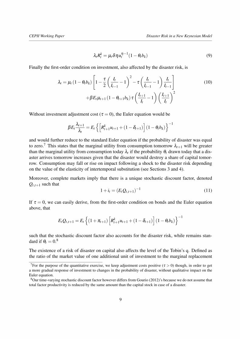
Finally the first-order condition on investment, also affected by the disaster risk, is

λt = µt (1−θtbk)

[1− τ

2

(It

It−1−1)2

− τ

(It

It−1−1)

ItIt−1

](10)

+βEt µt+1 (1−θt+1bk)τ

(It+1

It−1)(

It+1

It

)2

Without investment adjustment cost (τ = 0), the Euler equation would be

βEtλt+1

λt= Et

[Rk

t+1ut+1 +(1−δt+1)](1−θtbk)

−1

and would further reduce to the standard Euler equation if the probability of disaster was equalto zero.7 This states that the marginal utility from consumption tomorrow λt+1 will be greaterthan the marginal utility from consumption today λt if the probability θt drawn today that a dis-aster arrives tomorrow increases given that the disaster would destroy a share of capital tomor-row. Consumption may fall or rise on impact following a shock to the disaster risk dependingon the value of the elasticity of intertemporal substitution (see Sections 3 and 4).

Moreover, complete markets imply that there is a unique stochastic discount factor, denotedQt,t+1 such that

1+ it = (EtQt,t+1)−1 (11)

If τ = 0, we can easily derive, from the first-order condition on bonds and the Euler equationabove, that

EtQt,t+1 = Et

(1+πt+1)

[Rk

t+1ut+1 +(1−δt+1)](1−θtbk)

−1

such that the stochastic discount factor also accounts for the disaster risk, while remains stan-dard if θt = 0.8

The existence of a risk of disaster on capital also affects the level of the Tobin’s q. Defined asthe ratio of the market value of one additional unit of investment to the marginal replacement

7For the purpose of the quantitative exercise, we keep adjustment costs positive (τ > 0) though, in order to geta more gradual response of investment to changes in the probability of disaster, without qualitative impact on theEuler equation.

8Our time-varying stochastic discount factor however differs from Gourio (2012)’s because we do not assume thattotal factor productivity is reduced by the same amount than the capital stock in case of a disaster.

9


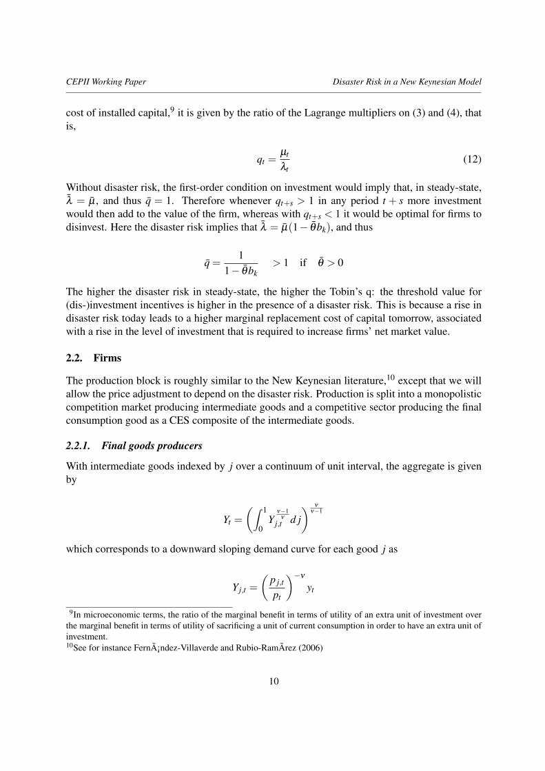
cost of installed capital,9 it is given by the ratio of the Lagrange multipliers on (3) and (4), thatis,

qt =µt

λt(12)

Without disaster risk, the first-order condition on investment would imply that, in steady-state,λ = µ , and thus q = 1. Therefore whenever qt+s > 1 in any period t + s more investmentwould then add to the value of the firm, whereas with qt+s < 1 it would be optimal for firms todisinvest. Here the disaster risk implies that λ = µ(1− θbk), and thus

q =1

1− θbk> 1 if θ > 0

The higher the disaster risk in steady-state, the higher the Tobin’s q: the threshold value for(dis-)investment incentives is higher in the presence of a disaster risk. This is because a rise indisaster risk today leads to a higher marginal replacement cost of capital tomorrow, associatedwith a rise in the level of investment that is required to increase firms’ net market value.

2.2. Firms

The production block is roughly similar to the New Keynesian literature,10 except that we willallow the price adjustment to depend on the disaster risk. Production is split into a monopolisticcompetition market producing intermediate goods and a competitive sector producing the finalconsumption good as a CES composite of the intermediate goods.

2.2.1. Final goods producers

With intermediate goods indexed by j over a continuum of unit interval, the aggregate is givenby

Yt =

(∫ 1

0Y

ν−1ν

j,t d j) ν

ν−1

which corresponds to a downward sloping demand curve for each good j as

Yj,t =

(p j,t

pt

)−ν

yt

9In microeconomic terms, the ratio of the marginal benefit in terms of utility of an extra unit of investment overthe marginal benefit in terms of utility of sacrificing a unit of current consumption in order to have an extra unit ofinvestment.10See for instance FernÃ¡ndez-Villaverde and Rubio-RamÃrez (2006)

10


and to an aggregate price index given by

pt =

(∫ 1

0p1−ν

j,t d j) 1

1−ν

2.2.2. Intermediate goods producers

Intermediate goods are produced with capital and labor, according to a standard Cobb-Douglasproduction function

Yj,t = AtKαj,tL

1−α

j,t

in which the capital leased to the firms is

Kt = utKt (13)

where ut is the variable utilization rate of capital, and in which total factor productivity, denotedAt , is driven by

logAt = (1−ρA) log A+ρA logAt−1 +σAεAt (14)

where the shocks are small and normally distributed (εt is i.i.d. N(0,1)).

There is a two-step problem for firms producing the intermediate goods. First, each firm jminimizes capital and labor costs at each date, independently of price adjustment, subject tothe restriction of producing at least as much as the intermediate good is demanded at the sellingprice, that is,

minL j,t ,K j,t

pt(wtL j,t +Rkt K j,t)

s.t. AtKαj,tL

1−α

j,t ≥(

p j,t

pt

)−ν

Yt

The first-order conditions for this problem give a capital-labor ratio which holds at the aggregatelevel since it is the same across all firms

(K j,t

L j,t

)∗=

wt

Rkt

α

(1−α)

and allows to write the optimal marginal input costs as

mc∗t = w1−αt

(1

1−α

)1−α( 1α

)α Rαt

At

11


from which the aggregate first-order conditions are expressed as

wt = mc∗ (1−α)At

(Kt

Lt

)α

(15)

Rkt = mc∗αAt

(Kt

Lt

)α−1

(16)

Then, given the optimal input mix, some firms maximize their profits by choosing their sellingprice p j,t . We consider two alternative ways to introduce nominal stickiness. One is standardCalvo time-dependent pricing so that firms in the intermediate sector face a constant probabilityζ0 of being unable to change their price at each time t despite the disaster risk. The other oneis to assume that firms’ price adjustment increases in the aggregate risk, i.e. the gap betweenthe current value of the probability ζt of being unable to change one’s price and the Calvoprobability ζ0 is given by

ζt−ζ0 =−θιt

where ι is the elasticity of the gap to the probability of disaster.11 12

Writing ζ as standing either for ζ0 in the first case or for ζt in the second, the profit-maximizingproblem in both cases is

maxp j,t

Et

∞

∑s=0

(ζ )s Qt+s

((p j,t

pt+s

)1−ν

yt+s−mc∗t+s

(p j,t

pt+s

)−ν

yt+s

)

The solution to this problem holds at the aggregate level (p∗t = p∗j,t). The gap between thisoptimal price p∗t and the consumer price index pt is

p∗tpt

=ν

ν−1Et

∑∞s=0 (ζ )

s Qt+s

(pt+spt

)ν

Yt+smc∗t+s

∑∞s=0 (ζ )

s Qt+s

(pt+spt

)ν−1Yt+s

11Note that this function requires to impose a parameter restriction so that ζ remains positive. With θ = 0.01 inparticular, ι cannot be lower than 0.05.12This price setting reminds the ‘SS pricing’ literature (Caplin and Leahy, 1991) although the firms do not react tothe effective realization of aggregate shocks but to the expected risk. This is because the probability of disaster isincorporated in the forward-looking agents’ optimization problem and the size of an effective disaster is constanthere.

12


This expression can finally be rewritten recursively in order to stress out the price adjustmentdynamics and in terms of an inflation gap to allow for a non-zero inflation steady-state, suchthat

1+π∗t1+πt

=ν

ν−1Et

Ξ1t/pνt

Ξ2t/pν−1t

(17)

with πt =pt

pt−1−1 the net inflation rate, π∗t the net reset inflation rate, and

Ξ1t

pνt=

Qt+s

βYtmc∗t +ζ βEt

Ξ1t+1

pνt+1

(1+πt+1)ν , and (18)

Ξ2t

pν−1t

=Qt+s

βYt +ζ βEt

Ξ2t+1

pν−1t+1

(1+πt+1)ν−1 (19)

All the computational details are given in Appendix.

2.3. Public authority

The public authority consumes some output Gt , charges lump sum taxes Tt to households, andissues debt Dt which pays interest it set up according to a standard Taylor-type rule that dependson the deviation of inflation from steady-state and on an output growth gap as

it = ρiit−1 +(1−ρi) [ψπ(πt− π)+ψY (yt− y)+ i]+σiεit (20)

in which y is the growth rate of output and where an overbar indicates the steady-state value ofa variable. The public authority’s budget constraint equates spending plus payment on existingdebt to collected taxes plus new debt issuance13, that is,

Gt +(1+ it)Dt

pt= Tt +

Dt+1

pt

in which Gt follows a first-order autoregressive process in the logs

logGt = (1−ρG) log(ωY )+ρG logGt−1 +σGεGt (21)

where ω is the steady-state share of output devoted to public expenditures.

13We assume that there is no money, hence no seignorage revenue in the model.

13


3. EQUILIBRIUM

3.1. Market clearing

Market-clearing in the bond market implies that the total amount of debt is equal to the totalamount of bounds in period t

Dt = Bt

and market-clearing in output implies that

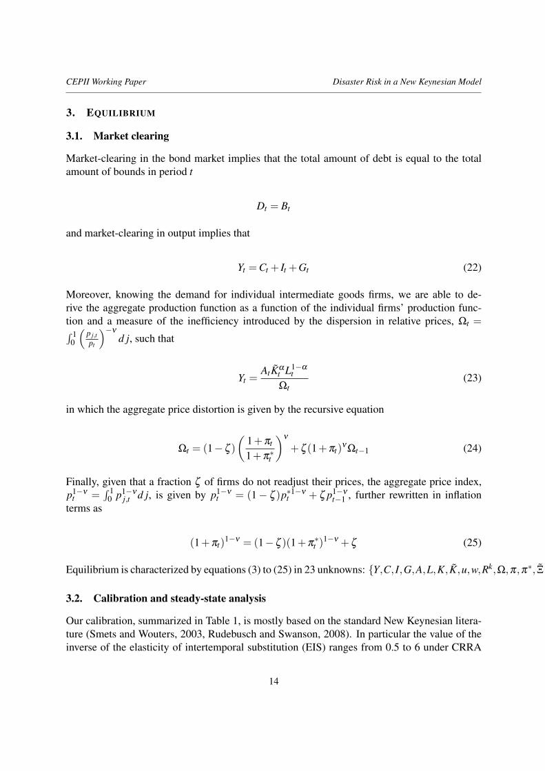
Yt =Ct + It +Gt (22)

Moreover, knowing the demand for individual intermediate goods firms, we are able to de-rive the aggregate production function as a function of the individual firms’ production func-tion and a measure of the inefficiency introduced by the dispersion in relative prices, Ωt =∫ 1

0

(p j,tpt

)−ν

d j, such that

Yt =AtKα

t L1−αt

Ωt(23)

in which the aggregate price distortion is given by the recursive equation

Ωt = (1−ζ )

(1+πt

1+π∗t

)ν

+ζ (1+πt)νΩt−1 (24)

Finally, given that a fraction ζ of firms do not readjust their prices, the aggregate price index,p1−ν

t =∫ 1

0 p1−ν

j,t d j, is given by p1−νt = (1− ζ )p∗1−ν

t + ζ p1−ν

t−1 , further rewritten in inflationterms as

(1+πt)1−ν = (1−ζ )(1+π

∗t )

1−ν +ζ (25)

Equilibrium is characterized by equations (3) to (25) in 23 unknowns: Y,C, I,G,A,L,K, K,u,w,Rk,Ω,π,π∗, Ξ1, Ξ2,mc∗,λ ,µ, i,q,Q,θ.

3.2. Calibration and steady-state analysis

Our calibration, summarized in Table 1, is mostly based on the standard New Keynesian litera-ture (Smets and Wouters, 2003, Rudebusch and Swanson, 2008). In particular the value of theinverse of the elasticity of intertemporal substitution (EIS) ranges from 0.5 to 6 under CRRA

14


preferences with a baseline value of 2. In addition, Barro (2006) found on historical data thatthe average share of capital that is destroyed in case of disaster is 43%, while Gourio (2012)estimates that the average probability of a such a disaster is 1.7% annually, backing it out fromevidence on asset prices under the assumption that the fall in total factor productivity is also ex-actly equal to 43%. Since we use the quarterly calibration of standard New Keynesian modelsand are not able to replicate the estimation so far, we test for several values of θ around a 1%benchmark, as well as for several values of bk and of the persistence in the shock to θ , withoutsignificant changes in our results.

In our steady-state, the capital stock, output, and consumption are lower in the presence of a dis-aster risk as compared to the same economy without disaster for all values of risk aversion/EIS.Steady-state investment and labor may be larger in the presence of disasters if the EIS is veryhigh (γ = 0.5), but are generally weaker, such that wages are generally lower. The firms cansubstitute labor to capital such that their steady-state marginal costs are unchanged even thoughthe cost of capital is higher in case of disaster. Therefore the non-zero steady-state inflationrate is unaffected by disaster risk and equal to the public authority’s target that we set at 2%annually. The main ratios, C/Y , I/Y , G/Y are in all cases slightly above or below their stan-dard values, 60%, 20% and 20%, respectively. Finally, the steady-state risk premium in caseof disaster corresponds to the wedge between the higher steady-state return on capital and theunchanged riskfree rate.

Gourio (2012) found that the model quantities shift to a lower steady-state in the economy withdisaster risk (as compared to an economy without disaster) if and only if the EIS is larger thanunity. Therefore, it is noteworthy to clarify at this point why we do get a lower steady-state forall values of the EIS here, on the one hand, and its further implications on the model dynam-ics, on the other hand. First, with Epstein-Zin preferences, i.e. dissociating the risk aversioncoefficient from the inverse of the EIS, it would be possible to show that, when investment oncapital becomes riskier, the risk-adjusted return on capital goes down for risk averse agents,while the effect of this change on the consumption-savings decisions depends on the value ofthe EIS (Weil, 1990, Angeletos, 2007). In particular, when the EIS is larger than unity (γ < 1),the substitution effect of a higher risk-adjusted return is larger than the income effect and sav-ings fall. Therefore the steady-state capital stock and output are lower. However, when the EISis equal to 1, both effects cancel each other out and savings are unaffected by changes in therisk-adjusted return, that is, are unaffected by changes in the return on capital even if agentsare risk-averse.14 Our specification, where risk aversion is only the inverse of the EIS, does notallow to disentangle the two effects, yet remains preferable in order to solve the equity premiumpuzzle by incorporating habit formation (Weil, 1989, Uhlig, 2007, Angeletos, 2007).

More importantly, the reason why we get lower steady-state macro quantities even when theEIS is unity is because we solve the model such that the disaster risk is treated as a small but

14The EIS determines the sign of the effect of increased uncertainty on savings while the risk aversion only affectsits magnitude (Weil, 1990).

15


certain probability of disaster instead of being a large uncertain shock. This allows to solvethe model quite easily without having to maintain Gourio’s assumption that the disaster is astrict combination of a depreciation shock to capital and a negative shock to the total factorproductivity by the same amount. Meanwhile, this does not substantially restrict our businesscycle analysis for two reasons. First, we capture the main first-moment effect of disaster riskby the fact that depreciation of capital will be higher in the future, even though we do nothave the second-moment effect associated with higher uncertainty about future depreciation.15

Second, Gourio shows that Tallarini (2000)’s observational equivalence in the dynamics ofthe macroeconomic variables in case there is an aggregate risk or not does not hold when theprobability of disaster is not constant. When the disaster risk is time-varying, Gourio finds thatrisk aversion matters for the macroeconomic dynamics, and this is captured here.

4. IMPULSE RESPONSES OF THE MACROECONOMIC VARIABLES

Analyzing the effects of a time-varying risk on asset pricing would require to treat the disas-ter risk as an uncertainty shock and to use nonlinear methods to solve the model. However,since there is a consensus about the irrelevance of approximation beyond the first-order for themacroeconomic quantities, on the one hand, and given that we do not consider the case of alarge shock, on the other hand, we maintain certainty-equivalence and first-order methods inthis version of the paper, although we keep track of some second-order corrections in the Ap-pendix.1617 For each (small) shock below, we compare the responses obtained in our model(solid line) to their counterpart in a flexible-price but otherwise similar model18 (dashed line)and in a standard sticky-price New Keynesian model without disaster risk (dotted line).

4.1. A rise in the probability of disaster

Figure 1 depicts the responses of the main variables to a rise in the probability of disaster,θ . Investment and capital fall on impact as households foresee the upcoming depreciation ofcapital when the probability of disaster, θ , rises. These effects are much more important underCalvo price stickiness (ζ = 0.8) than under flexible prices (ζ = 0) as all firms do not adjust theirprices downwards as much as they would optimally do to match the fall in aggregate demand.The capital stock still goes down next periods because of the depressed investment even thoughthe probability of disaster gradually returns to its initial level (from the autoregressive process).15Gourio admits that the two effects are present but cannot be disentangled in his article. In every case, both effectspush the variables in the same direction, and the first-moment effect is far more important for macroeconomicquantities.16Since certainty-equivalence holds, these correction terms are naturally very small.17The effective occurrence of a disaster would be a large shock, whereas the rise in the probability of disasterconsidered here is a small one.18The flexible-price model is different from Gourio’s RBC with disaster risk since we have CRRA preferenceswith habit formation, a public authority, and variable utilization rate of capital, on the one hand, and because wedo not assume a fall to TFP by the same amount as simultaneous to the rise in the probability of disaster, on theother hand.

16


Labor supply decreases when prices are flexible because it is less attractive for workers to worktoday when the return on savings is low (intertemporal effect), despite a negative wealth effectthat tends to push employment up.19 Wages thus slightly rise. However, when prices are sticky,the firms that cannot readjust their prices downwards as much as they want face an even lowerdemand for their own intermediate goods, and thus in turn lower their demand of labor, leadingwages to fall. Because capital and labor decrease more under sticky prices, combined with thefact that decrease in aggregate demand is more severe, the slump in output is far larger withnominal rigidity.

In the flexible case, consumption increases on impact as households substitute consumptionfor investment in the first period, while lower output leads consumption to fall in the nextperiods, for standard values of the EIS and/or risk aversion.20 With sticky prices however,consumption falls on impact for the baseline calibration (γ = 2), or lower values of the EIS(higher risk aversion). For very low risk aversion, consumption moves up on impact similarlyto the flexible-price case but a quantitative difference due to price stickiness remains, as shownin Figure 5.

As investment in capital is riskier, households’ demand for safer government bonds rises, sothat the short-term nominal interest rate falls (“flight to quality” effect). However, because ofthe inertia in the Taylor-type reaction, the interest rate — and therefore inflation — falls lessunder price stickiness Finally, actual inflation decreases less than reset inflation, so that the pricedispersion falls, but still falls more than the nominal interest rate, so that the real rate rises.

Figures 6 to 10 present some robustness checks and alternative specifications. Figure 6 con-siders different values of the steady-state probability of disaster (θ ). While the magnitude ofthe effects increases in the steady-state disaster risk, the qualitative responses are all identical.Figure 7 gives some alternative values for the persistence of the shock (ρθ ). Figure 8 tests fordifferent values for the share of capital which is destroyed in case of disaster (bk), including apossible negative value.21

More importantly, Figure 9 gives the responses under state-dependent price stickiness for dif-ferent values of the parameter ι < 1.22 The responses still differ significantly from the pureflexible-price version of the model (ζ = 0) and our main results hold, notably the drop in wages,including for an extreme ι = 0.1.

We finally consider a fall in the probability of disaster in Figure 10. Table 2 gives the second-order correction terms associated with this shock, naturally found to be very small under the

19The relative importance of the two effects would depend on the EIS with Epstein-Zin preferences. However thisresult is familiar with standard calibration of CRRA preferences.20Gourio (2012) found a similar effect with a slightly different flexible-price model and a simultaneous shock tothe TFP.21A negative value of bk verifies that the model works symmetrically such that the rare event could be a “miracle”instead of a “disaster”.22When ι ≥ 1, the responses are almost identical to the time-dependent pricing case.

17


certainty-equivalence assumption.

To sum up, a rise in the probability of disaster creates a recession, a fall in inflation, a flight toquality in terms of asset demand, depressed investment and labor, as well as lower consumptionfor standard risk aversion. The fact that the probability of a disaster is higher suffices to generatethis recession, without effective occurrence of the disaster.

4.2. Standard shocks

The responses to standard shocks in the model with disaster risk are very close to the responsesin a standard New Keynesian model.

For a TFP shock (Figure 2), output and investment rise because the marginal returns on laborand capital rise. However this is slightly less important in the presence of a disaster risk whichdepreciates capital. Consumption rise more however from the substitution effect between in-vestment and consumption for households. The response of labor is discussed extensively in theliterature: in opposition to a RBC where labor increases because the marginal return on labor ishigher, sticky prices prevent some firms from lowering their prices leading them to lower theirlabor demand because of the contraction in demand for their own intermediate goods (Galí,1999). In addition, higher incomes for households make leisure more desirable so that the sup-ply of labor does not substantially rise neither. As reset inflation is higher than actual inflation,price dispersion falls and the real interest rate goes up despite the fall in the nominal rate.

A positive shock to public expenditures (Figure 3) also replicates the very well-known reactions.In all cases, there is a temporary rise in output from the rise in aggregate demand, an evictioneffect on private consumption and investment, hence a fall in capital. Thus firms rely more onlabor and wages go up. High reset inflation creates more price dispersion, and the nominal rateis increased.

Finally, a monetary contraction (Figure 4) generates the standard decrease in all macro quanti-ties, as well as in inflation and price dispersion.

5. FURTHER RESEARCH

This paper provides a baseline framework that could be used to develop a number of innovativeresearch ideas, including the role of monetary policy to prevent self-fulfilling recessions in caseof misperceptions about the disaster risk. This Section presents our research agenda, whichbroadly consists in three steps.

First, we would like to account for a perceived risk of disaster along with the real disaster risk.Gourio (2012) considers that the probability of disaster introduced in his model (and in ours)may result from the economic agents’ perception, probably because considering that the prob-ability taken as given by the agents is the real risk would be associated with perfect individualrationality and knowledge about disasters while one could be more agnostic by considering it

18


as merely perceived, especially for rare events. We think that it would be helpful to build on thebehavioral macroeconomics literature (Gabaix and Laibson, 2002, De Grauwe, 2010, Fuster,Laibson and Mendel, 2010, Angeletos and La’O, 2012, Barsky and Sims, 2012) in order todisentangle a perceived from a real disaster risk. Another mean would be the use of computa-tional methods in order to keep the disaster variable (xt+1) as an indicator in the Euler equationinstead of substituting the time-varying probability θt of an effective future occurrence. Thiswould allow to simulate a rise in the probability of disaster while preventing the real occurrenceof a disaster by accounting for uncertainty in the model.

As a second step, we will evaluate the model predictions in terms of asset pricing, especiallythe countercyclicality of the risk premium. Some interactions between price rigidity and therisk of disaster may affect equity returns. The asset price volatility may in turn have importantconsequences on consumption volatility. In particular the perception of disaster risk may beone of the psychological mechanisms that alter the reactivity of consumption changes to assetprice movements (see Lynch, 1996, or Gabaix and Laibson, 2002, for instance), in addition tohabit formation (Campbell and Cochrane, 1999, Uhlig, 2007), or adjustment costs (Grossmanand Laroque, 1990). On practical grounds, pricing assets requires a few more sophisticationsin our setup. One is to go beyond the first-order approximation in the Taylor expansion. Theconsensus in the literature is that these higher-order terms do not matter for the responses ofmacroeconomic quantities we have focused on so far but have an important role in the assetpricing in the presence of a time-varying risk. Another key element will be to add corporatebonds in the model since leverage is a standard way to make equity returns more volatile andprocyclical — in line with the data — in the literature, which may be even more relevant in amodel in which firms’ prices are sticky.

Finally, we would like to assess the desirability of monetary policy to prevent a (self-fulfilling)recession from a sudden rise in the (perceived) probability of disaster. Several conventional andunconventional interventions could be compared with one another by incorporating a welfarefunction measuring their effectiveness. In particular we think of adding an extra term in theTaylor-type rule which would represent a direct response of the monetary authority in the faceof a wave of pessimism. This would be a quasi-conventional intervention, making changesin the nominal interest rate more reactive but still limited by the zero lower bound. A moreunconventional measure could consist in purchasing corporate bonds (which may encompassbank debt), directly affected by the disaster risk, by selling riskfree government bonds (as far assovereign default is excluded).

6. CONCLUSION

This paper provides a baseline framework to analyze the business cycle responses of macroeco-nomic quantities in the presence of a small time-varying disaster risk in an otherwise standardNew Keynesian model. While following Gourio (2012) on the description of an economic dis-aster, we relax the assumption that total factor productivity needs to fall by the same amount

19


than the capital stock in case of a disaster. By incorporating investment adjustment costs andmonopolistic competition, we show that the magnitude of the recession following a shock tothe probability of disaster may be far increased. As compared with the early papers on rareevents, we also account for the fact that consumption and wages do not rise in distressed eco-nomic times, whether nominal rigidity is time-dependent or state-dependent. More generally,this paper is a first step towards the introduction of rare events into the models used to conductmonetary policy, and will be used to compare the effectiveness of several interventions in thepresence of such a risk.

20


REFERENCES

George-Marios Angeletos. Uninsured idiosyncratic investment risk and aggregate saving. Review ofEconomic Dynamics, 10(1):1–30, January 2007.

George-Marios Angeletos and Jennifer La’O. Sentiments. Unpublished manuscript, available at http://faculty.chicagobooth.edu/jennifer.lao/research/sentiments.pdf.

Robert J. Barro. Rare disasters and asset markets in the twentieth century. Quarterly Journal of Eco-nomics, 2006.

Robert B. Barsky and Eric R. Sims. Information, animal spirits, and the meaning of innovations inconsumer confidence. American Economic Review, forthcoming, 2012.

Nicholas Bloom. The impact of uncertainty shocks. Econometrica, 77(3):623–685, 05 2009.

Craig Burnside and Martin Eichenbaum. Factor-hoarding and the propagation of business-cycle shocks.American Economic Review, 86(5):1154–74, December 1996.

John Campbell and John Cochrane. By force of habit: A consumption-based explanation of aggregatestock market behavior. Journal of Political Economy, 1999.

Andrew Caplin and John Leahy. State-dependent pricing and the dynamics of money and output. Quar-terly Journal of Economics, 106(3):683–708, August 1991.

Paul De Grauwe. Top-down versus bottom-up macroeconomics. CESifo Economic Studies, 56(4):465–497, December 2010.

Paul De Grauwe. Animal spirits and monetary policy. Economic Theory, 47(2):423–457, June 2011.

Jesús Fernández-Villaverde and Juan F. Rubio-Ramírez. A baseline DSGE model. Unpublishedmanuscript, available at http://economics.sas.upenn.edu/~jesusfv/benchmark_DSGE.

pdf, year = 2006.

Andreas Fuster, Benjamin Hebert, and David Laibson. Natural expectations, macroeconomic dynamics,and asset pricing. NBER Working Papers 17301, National Bureau of Economic Research, Inc,August 2011.

Andreas Fuster, David Laibson, and Brock Mendel. Natural expectations and macroeconomic fluctua-tions. Journal of Economic Perspectives, 24(4):67–84, 2010.

Xavier Gabaix. Variable rare disasters: An exactly solved framework for ten puzzles in macro-finance.Quarterly Journal of Economics, 127(2):645–700, 2012.

Xavier Gabaix and David Laibson. The 6D bias and the equity-premium puzzle. In NBER Macroeco-nomics Annual 2001, Volume 16, NBER Chapters, pages 257–330. National Bureau of EconomicResearch, Inc, 2002.

21

http://faculty.chicagobooth.edu/jennifer.lao/research/sentiments.pdf

http://faculty.chicagobooth.edu/jennifer.lao/research/sentiments.pdf

http://economics.sas.upenn.edu/~jesusfv/benchmark_DSGE.pdf

http://economics.sas.upenn.edu/~jesusfv/benchmark_DSGE.pdf


Jordi Galí. Technology, employment, and the business cycle: Do technology shocks explain aggregatefluctuations? American Economic Review, 89(1):249–271, March 1999.

François Gourio. Disasters and recoveries. American Economic Review, 98(2):68–73, May 2008.

François Gourio. Disaster risk and business cycles. American Economic Review, forthcoming, 2012.

Sanford J. Grossman and Guy Laroque. Asset pricing and optimal portfolio choice in the presence ofilliquid durable consumption goods. Econometrica, 58(1):25–51, January 1990.

Anthony W. Lynch. Decision frequency and synchronization across agents: Implications for aggregateconsumption and equity return. Journal of Finance, 51(4):1479–97, September 1996.

Nicolas Petrosky-Nadeau. TFP during a credit crunch. GSIA working papers, Carnegie Mellon Univer-sity, Tepper School of Business, 2010.

Thomas A. Rietz. The equity risk premium: a solution. Journal of Monetary Economics, 22(1):117–131,July 1988.

Glenn D. Rudebusch and Eric T. Swanson. Examining the bond premium puzzle with a dsge model.Journal of Monetary Economics, 55:S111–S126, October 2008.

Frank Smets and Rafael Wouters. An estimated dynamic stochastic general equilibrium model of theeuro area. Journal of the European Economic Association, 1(5):1123–1175, 09 2003.

Thomas D. Tallarini Jr. Risk-sensitive real business cycles. Journal of Monetary Economics, 45(3):507–532, June 2000.

Harald Uhlig. Explaining asset prices with external habits and wage rigidities in a dsge model. AmericanEconomic Review, 97(2):239–243, May 2007.

Philippe Weil. The equity premium puzzle and the risk-free rate puzzle. Journal of Monetary Economics,24(3):401–421, November 1989.

Philippe Weil. Nonexpected utility in macroeconomics. Quarterly Journal of Economics, 105(1):29–42,February 1990.

22


APPENDIX

8. MATHEMATICAL APPENDIX

A. Households

Given that next period disaster xt+1 is equal to 1 with probability θt and equal to 0 with proba-bility 1−θt , the law of accumulation of capital can be rewritten as

Kt+1 = [θt(1−bk)+(1−θt)](1−δt)Kt +[1−S(It/It−1)]It= (1−θtbk)(1−δt)Kt +[1−S(It/It−1)]It

Therefore the Lagrangian for the households’ problem is

L =Et

∞

∑t=0

βt

((Ct −hCt−1)

1−γ

1− γ−χ

L1+φ

t

1+φ

)

+λt

(WtLt +(1+ it−1)

Bt

pt+

Mt

pt− Bt+1

pt−Mt+1

pt+Rk

t utKt +Πt −Tt − It −Ct

)+ µt

[((1−δuη

t )Kt +

(1− τ

2

(It

It−1−1)2)

It

)(1−θtbk)−Kt+1

]

and the first-order conditions are

• Consumption: λt = (Ct−hCt−1)−γ −βhEt(Ct+1−hCt)

−γ

• Labor: χLφ

t = wtλt• Bonds: λt = βEtλt+1(1+ it)(1+πt+1)

−1, with1+πt+1 ≡ pt+1pt

• Capital: µt = βEt[λt+1Rk


t+1)(1−θt+1bk)

]• Capital utilization rate: λtRk

t = µtδηuη−1t (1−θtbk)

• Investment: λt = µt (1−θtbk)

[1− τ

2

(It

It−1−1)2− τ

(It

It−1−1)

ItIt−1

]+βEt µt+1 (1−θt+1bk)τ

(It+1It−1)(

It+1It

)2

With no investment adjustment cost (τ = 0), the FOC on investment becomes λt = µt(1−θtbk),which in turn implies from the FOC on the capital utilization rate that Rk

t = δ ′t . Substituting intothe FOC on capital gives the Euler equation (11) in case τ = 0.

B. Firms

• Production aggregation

23


The aggregate of intermediate goods is given by

Yt =

(∫ 1

0Y

ν−1ν

j,t d j) ν

ν−1

so that the profit maximization problem of the representative firm in the final sector is

maxYt, j

pt

(∫ 1

0Y

ν−1ν

j,t d j) ν

ν−1

−∫ 1

0p j,tYj,td j

The first-order condition with respect to Yt, j yields a downward sloping demand curve for eachintermediate good j as

Yj,t =

(p j,t

pt

)−ν

Yt

The nominal value of the final good is the sum of prices times quantities of intermediates

ptYt =∫ 1

0p j,tYj,td j

in which Yt is substituted to give the aggregate price index as

pt =

(∫ 1

0p1−ν

j,t d j) 1

1−ν

• Cost minimization

Firms are price-takers in the input markets, facing a nominal wage wt pt and a nominal rentalrate Rk

t pt (wt and Rkt are in real terms). Therefore, they choose the optimal quantities of labor

and capital given the input prices and subject to the restriction of producing at least as much asthe intermediate good is demanded at the given price. The intratemporal problem is

minL j,t ,K j,t

wt ptL j,t +Rkt ptK j,t

s.t. atKαj,tL

1−α

j,t ≥(

p j,t

pt

)−ν

Yt

The first-order conditions are

24


(L j,t :) wt =ϕ j,t

pt(1−α)At

(K j,t

L j,t

)α

(K j,t :) Rkt =

ϕ j,t

ptαAt

(K j,t

L j,t

)α−1

in which the Lagrange multiplier ϕ j,t can be interpreted as the (nominal) marginal cost associ-ated with an additional unit of capital or labor. Rearranging gives the optimal capital over laborratio as

(K j,t

L j,t

)∗=

wt

Rkt

α

(1−α)

in which none of the terms on the right hand side depends on j, and thus holds for all firms inequilibrium, i.e., Kt

Lt=

K j,tL j,t

. Replacing in the first-order conditions further gives mc∗t =ϕtpt

as

mc∗t = w1−αt

(1

1−α

)1−α( 1α

)α(Rk

t)α

At

• Profit maximization

Let us now consider the pricing problem of a firm that gets to update its price in period t andwants to maximize the present discounted value of future profits. First, the (nominal) profit flow,p j,tYj,t −wt ptL j,t −Rk

j,t ptK j,t , can be rewritten as Π j,t = (p j,t −ϕt)Yj,t , that is, in real terms,Π j,tpt

=p j,tpt

Yj,t −mc∗t Y j,t . Firms will discount future profit flows by both the stochastic discountfactor, Qt = β sλt+s, and by the probability ζ s that a price chosen at time t is still in effect at

time s. Replacing Yj,t =(

p j,tpt

)−ν

Yt , the profit maximization problem is

maxp j,t

Et

∞

∑s=0

(ζ )s Qt+s

((p j,t

pt+s

)1−ν

Yt+s−mc∗t+s

(p j,t

pt+s

)−ν

Yt+s

)

Given that mc∗t =ϕtpt

and factorizing, we can rewrite it as

maxp j,t

Et

∞

∑s=0

(ζ )s Qt+s pν−1t+s Yt+s

(p1−ν

j,t −ϕt p−ν

j,t

)The first-order condition is

25


Et

∞

∑s=0

(ζ )s Qt+s pν−1t+s Yt+s

((1−ν)p−ν

j,t +νϕt p−ν−1j,t

)= 0

which simplifies as

p∗j,t =ν

ν−1Et

∑∞s=0 (ζ )

s Qt+s pνt+sYt+smc∗t+s

∑∞s=0 (ζ )

s Qt+s pν−1t+s Yt+s

Note that this optimal price depends on aggregate variables only, so that p∗t = p∗j,t . The gapbetween the current price and the optimal aggregate price is thus given by

p∗tpt

=ν

ν−1Et

∑∞s=0 (ζ )

s Qt+s

(pt+spt

)ν

Yt+smc∗t+s

∑∞s=0 (ζ )

s Qt+s

(pt+spt

)ν−1Yt+s

In order to stress out the recursive price adjustment, let define p∗t as

p∗t =ν

ν−1Et

Ξ1t

Ξ2t

in which Ξ1t and Ξ2t can be expressed recursively as

Ξ1t = Qt+s pνt Ytmc∗t +ζ EtΞ1t+1

Ξ2t = Qt+s pν−1t Yt +ζ EtΞ2t+1

and rewritten as

βΞ1t

pνt= Qt+sYtmc∗t +ζ β

2EtΞ1t+1

pνt+1

(pt+1

pt

)ν

βΞ2t

pν−1t

= Qt+sYt +ζ β2Et

Ξ2t+1

pν−1t+1

(pt+1

pt

)ν−1

Therefore, we have

26


p∗tpt

=ν

ν−1Et

Ξ1tpν

tΞ2t

pν−1t

C. Aggregation

C.1. Bonds market

Market-clearing requires that:Dt = Bt

C.2. Aggregate demand

First replace Dt = Bt into the public authority’s budget constraint, and express Tt as

Tt = Gt +(1+ it)Bt

pt− Bt+1

pt

which can be plugged into the household budget constraint as

Ct + It +Bt+1

pt= wtLt +(1+ it)

Bt

pt+Rk

t Kt +Πt−(

Gt +(1+ it)Bt

pt− Bt+1

pt

)This further simplifies to:

Ct + It +Gt = wtLt +Rkt Kt +Πt

where we have to verify that the RHS is equal to Yt . Total profits Πt must be equal to the sumof profits earned by intermediate good firms, that is

Πt =∫ 1

0Π j,td j

Real profits earned by intermediate good firms j are given by

Π j,t(real) =p j,t

ptYj,t−wtL j,t−Rk

t K j,t

Substituting Y j,t , we have

27


Π j,t(real) =

(p j,t

pt

)1−ν

Yt−wtL j,t−Rkt K j,t

Therefore,

Πt(real) =∫ 1

0

((p j,t

pt

)1−ν

Yt −wtL j,t −Rkt K j,t

)d j =

∫ 1

0

(p j,t

pt

)1−ν

Ytd j

−∫ 1

0wtL j,td j−

∫ 1

0Rk

t K j,td j

Πt(real) =∫ 1

0

((p j,t

pt

)1−ν

Yt −wtL j,t −Rkt K j,t

)d j = Yt

1p1−ν

t

∫ 1

0(p j,t)

1−ν d j

−wt

∫ 1

0L j,td j−Rk

t

∫ 1

0K j,td j

Given that

- the aggregate price level is p1−νt =

∫ 10 p1−ν

j,t d j,- aggregate labor demand must equal supply,

∫ 10 L j,td j = Lt , and

- aggregate supply of capital services must equal demand∫ 1

0 K j,td j = Kt ,

the aggregate profit is

Πt(real) = Yt−wtLt−Rkt Kt

Plugging this expression into the household budget constraint finally gives the aggregate ac-counting identity as

Yt =Ct + It +Gt

C.3. Inflation

Firms have a probability 1− ζ of getting to update their price each period. Since there are aninfinite number of firms, there is also the exact fraction 1− ζ of total firms who adjust theirprices and the fraction ζ who stay with the previous period price. Moreover, since there is arandom sampling from the entire distribution of firm prices, the distribution of any subset of

28


firm prices is similar to the entire distribution. Therefore, the aggregate price index, p1−νt =∫ 1

0 p1−ν

j,t d j, is rewritten as

p1−νt =

∫ 1−ζ

0p∗1−ν

t d j+∫ 1

1−ζ

p1−ν

j,t−1d j

which simplifies top1−ν

t = (1−ζ )p∗1−νt +ζ p1−ν

t−1

Dividing both sides of the equation by p1−ν

t−1

(pt

pt−1

)1−ν

= (1−ζ )

(p∗t

pt−1

)1−ν

+ζ

(pt−1

pt−1

)1−ν

and defining gross inflation as 1+πt =pt

pt−1and gross reset inflation as 1+π∗t =

p∗tpt−1

, we get

(1+πt)1−ν = (1−ζ )(1+π

∗t )

1−ν +ζ

Finally, from p∗t =ν

ν−1EtΞ1tΞ2t

, we have

p∗tpt

=ν

ν−1Et

Ξ1t/pνt

Ξ2t/pν−1t

Rewritting the left-hand side as p∗tpt

pt−1pt−1

, and rearranging, we get

π∗t = πt

ν

ν−1Et

Ξ1t/pνt

Ξ2t/pν−1t

Therefore we have

Ξ1t

pνt=

Qt+s

βYtmc∗t +ζ βEt

Ξ1t+1

pνt+1

(1+πt+1)ν

Ξ2t

pν−1t

=Qt+s

βYt +ζ βEt

Ξ2t+1

pν−1t+1

(1+πt+1)ν−1

29


C.4. Aggregate supply

We know that the demand to individual firm j is given by

Yj,t =

(p j,t

pt

)−ν

Yt

and that firm j hires labor and capital in the same proportion than the aggregate capital tolabor ratio (common factor markets). Hence, substituting in the production function for theintermediate good j we get

At

(Kt

Lt

)α

L j,t =

(p j,t

pt

)−ν

Yt

Then, summing up across the intermediate firms gives

At

(Kt

Lt

)α ∫ 1

0L j,td j = Yt

∫ 1

0

(p j,t

pt

)−ν

d j

Given that aggregate labor demand equals aggregate labor supply∫ 1

0 L j,td j = Lt , we have

∫ 1

0

(p j,t

pt

)−ν

d jYt = AtKαt L1−α

t

Thus, the aggregate production function can be written as

Yt =AtKα

t L1−αt

Ωt

where Ωt =∫ 1

0

(p j,tpt

)−ν

d j measures a distortion introduced by the dispersion in relative prices.23

In order to express Ωt in aggregate terms, let decompose it according to the Calvo pricing as-sumption again, so that

Ωt =∫ 1

0

(p j,t

pt

)−ν

d j = pνt

∫ 1

0p−ν

j,t

23This distortion is not the one associated with the monopoly power of firms but an additional one that arises fromthe relative price fluctuations due to prie stickiness.

30


pνt

∫ 1

0p−ν

j,t = pνt

(∫ 1−ζ

0p∗−ν

t d j+∫ 1

1−ζ

p−ν

j,t−1d j)

pνt

∫ 1

0p−ν

j,t = pνt (1−ζ )p∗−ν

t + pνt

∫ 1

1−ζ

p−ν

j,t−1d j

pνt

∫ 1

0p−ν

j,t = (1−ζ )

(p∗tpt

)−ν

+ pνt

∫ 1

1−ζ

p−ν

j,t−1d j

pνt

∫ 1

0p−ν

j,t = (1−ζ )

(p∗t

pt−1

)−ν( pt−1

pt

)−ν

+ pνt

∫ 1

1−ζ

p−ν

j,t−1d j

pνt

∫ 1

0p−ν

j,t = (1−ζ )(1+π∗t )−ν(1+πt)

ν + p−ν

t−1 pνt

∫ 1

1−ζ

(p j,t−1

pt−1

)−ν

d j

Given random sampling and the fact that there is a continuum of firms

Ωt = (1−ζ )(1+π∗t )−ν(1+πt)

ν +ζ (1+πt)νΩt−1

D. Full set of equilibrium conditions

Kt+1 =

(1−δuη

t )Kt +

[1− τ

2

(It

It−1−1)2]

It

(1−θtbk) (26)

logθt = (1−ρθ ) log θ +ρθ logθt−1 +σθ εθt (27)

Kt = utKt (28)

λt = (Ct−hCt−1)−γ −βhEt(Ct+1−hCt)

−γ (29)

χLφ

t = wtλt (30)

λt = βEtλt+1(1+ it+1)(1+πt+1)−1 (31)

31


µt = βEt

[λt+1Rk


t+1)(1−θt+1bk)

](32)

λtRkt = µtδηuη−1

t (1−θtbk) (33)

λt = µt (1−θtbk)

[1− τ

2

(It

It−1−1)2

− τ

(It

It−1−1)

ItIt−1

]

+βEt µt+1 (1−θt+1bk)τ

(It+1

It−1)(

It+1

It

)2

(34)

1+ it = (EtQt,t+1)−1 (35)

qt =µt

λt(36)

logAt = (1−ρA) log A+ρA logAt−1 +σAεAt (37)

wt = mc∗ (1−α)At

(Kt

Lt

)α

(38)

Rkt = mc∗αAt

(Kt

Lt

)α−1

(39)

(1+π∗t ) = (1+πt)

ν

ν−1Et

Ξ1t

Ξ2t

(40)

where Ξ1t =Ξ1tpν

tand Ξ2t =

Ξ2tpν−1

t.

Ξ1t = λtYtmc∗t +ζ βEtΞ1t+1 (1+πt+1)ν (41)

Ξ2t = λtYt +ζ βEtΞ2t+1 (1+πt+1)ν−1 (42)

32


it = ρiit−1 +(1−ρi) [ψπ(πt− π)+ψY (yt− y)+ i]+σiεit (43)

logGt = (1−ρG) log(ωY )+ρG logGt−1 +σGεGt (44)

Yt =Ct + It +Gt (45)

Yt =AtKαL1−α

t

Ωt(46)

(1+πt)1−ν = (1−ζ )(1+π

∗t )

1−ν +ζ (47)

Ωt = (1−ζ )(1+π∗t )−ν(1+πt)

ν +ζ (1+πt)νΩt−1 (48)

This is a system of 23 equations in 23 unknowns: Y,C, I,G,A,L,K, K,u,w, Rk,Ω,π,π∗, Ξ1, Ξ2,mc∗,λ ,µ, i,q,Q,θ.

E. Steady-state

From the FOC on investment (34), we have

λ = µ(1− θbk) (49)

which implies by (36) that

q =µ

λ=

11− θbk

(50)

Without disaster risk, we would have q = 1 determining the threshold under which firms investor disinvest to raise their market value. Here disaster risk implies that this threshold is greaterthan unity since, for a given replacement cost in terms of utility, firms find it less profitable toinvest as the probability that a part of their capital turns out to be destroyed rises.

Normalizing u = 1, we have ¯K = K from (28), and from (33)

Rk = δη (51)

33


Moreover (32) implies that

Rk =1

β (1− θbk)− (1−δ ) (52)

The last two equations imply a parameter restriction of η as

η = 1+1

β (1−θbk)−1

δ(53)

Therefore, with parameter values β = .99, δ = .025, θ = .017, and bk = .43, we have η = 1.7(and η = 1.404 in a world without disasters).

Then from (47), and given the target inflation rate π , we have the steady-state reset inflation rateas

(1+ π∗) =

((1+ π)1−ν −ζ

1−ζ

) 11−ν

(54)

and, since from (40) we have,

(1+ π∗) = (1+ π)

ν

ν−1

¯Ξ1¯Ξ1

(55)

where, from (41) and (42),

¯Ξ1 =

λY mc∗

1−ζ β (1+ π)ν(56)

¯Ξ2 =

λY1−ζ β (1+ π)ν−1 (57)

we get

(1+ π∗) = (1+ π)

ν

ν−1mc∗

1−ζ β (1+ π)ν−1

1−ζ β (1+ π)ν(58)

34


which gives the steady-state marginal cost mc∗ as

mc∗ =ν−1

ν

1(1+ π)

1−ζ β (1+ π)ν

1−ζ β (1+ π)ν−1

((1+ π)1−ν −ζ

1−ζ

) 11−ν

(59)

Note that we must therefore restrict parameter values so that ζ β (1+ π)ν < 1.

With the expressions for Rk and mc∗, we can express the steady-state capital-labor ratio as afunction of the steady-state characteristics of disaster from (39)

KL=

(mc∗α a

Rk

) 11−α

(60)

Therefore the steady-state wage is given by (38)

w = mc∗(1−α)a(

KL

)α

(61)

From (48), we have

Ω =(1−ζ )(1+ π∗)−ν(1+ π)ν

1−ζ (1+ π)ν(62)

From the law of capital accumulation (26) in steady-state, we have

I = K(

11− θbk

− (1−δ )

)(63)

and given that from (44),G = ωY (64)

the accounting identity (45) becomes in steady-state

Y =1

1−ω

C+ K

[1

1− θbk− (1−δ )

](65)

in which 11−ω

is the keynesian multiplier of public expenditures. Further dividing each side byL gives

YL=

11−ω

CL+

KL

[1

1− θbk− (1−δ )

](66)

35


Replacing the left-hand side by the output-labor ratio obtained from the aggregate productionfunction (46), we have

AΩ

(KL

)α

=1

1−ω

CL+

KL

[1

1− θbk− (1−δ )

](67)

which can be solved for the steady-state consumption-labor ratio as

CL=

A(1−ω)

Ω

(KL

)α

− KL

[1

1− θbk− (1−δ )

](68)

Combining the FOC on consumption (29) in steady-state

λ = [(1−h)C]−γ(1−βh) (69)

with the FOC on labor (30) in steady-state

L =

(wλ

χ

)1/φ

(70)

we can express L as a function of the steady state consumption-labor ratio

L =

w(1−h)−γ

(CL

)−γ

(1−βh)

χL

1

φL+γ

(71)

which gives λ by (69) and therefore µ . L also gives Y by (66) and K by (60). Then G is obtainedby (64) and I by the accounting identity or by (63). Then we get ¯

Ξ1 and ¯Ξ2 by (56) and (57).

Finally, from the FOC on bonds (31) we have the standard Fisher relation between the subjectivediscount factor, the nominal interest rate and the inflation rate, 1/β = (1+ i)/(1+ π), such that,by (35), the one-period stochastic discount factor is

Q =1

1+ i=

β

1+ π(72)

36


Figure E.1 – Standard-deviation responses to a shock to the probability of disaster (increasein θ ). Solid line: model with disaster risk and sticky prices (ζ = 0.8). Dashed line: model with disasterrisk and flexible prices (ζ = 0).


Table E.1 – Baseline calibration parameters (quarterly values)

Utility functionβ discount factor 0.99γ inverse of EIS / risk aversion coefficient 2h habit in consumption 0.7φ inverse of the elasticity of work effort to the real wage 1χ labor disutility weight 4.74

Investmentδ capital depreciation rate 0.025τ investment adjustment costs 0.5u utilization rate of capital 1

Productionα capital share of production 0.33ζ0 Calvo probability 0.8ν elasticity of substitution among intermediate goods 6

Public authorityω steady-state G/Y ratio 0.2ψπ Taylor rule inflation weight 1.5ψY Taylor rule output weight 0.5π target inflation rate 0.005ρA TFP smoothing parameter 0.9ρG government expenditures smoothing parameter 0.85ρi interest rate smoothing parameter 0.85

Disaster riskθ disaster risk 0.01bk share of capital destroyed if disaster 0.43ρθ disaster risk smoothing parameter 0.85σ standard deviation of shocks 0.01


Figure E.2 – Standard-deviation responses to a productivity shock. Solid line: model with dis-aster risk and sticky prices (ζ = 0.8). Dashed line: model with disaster risk and flexible prices (ζ = 0).Dotted line: model without disasters, with sticky prices.


Figure E.3 – Standard-deviation responses to a public spending shock. Solid line: model withdisaster risk and sticky prices (ζ = 0.8). Dashed line: model with disaster risk and flexible prices (ζ =0). Dotted line: model without disasters, with sticky prices.


Figure E.4 – Standard-deviation responses to a monetary shock. Solid line: model with disasterrisk and sticky prices (ζ = 0.8). Dashed line: model with disaster risk and flexible prices (ζ = 0). Dottedline: model without disasters, with sticky prices.


Figure E.5 – Standard-deviation of consumption to a shock to the probability of disaster, fordifferent values of the risk aversion coefficient γ .

Figure E.6 – Standard-deviation responses to a shock to the probability of disaster, for differentvalues of the steady-state probability of disaster, θ .


Figure E.7 – Standard-deviation responses to a shock to the probability of disaster, for differentvalues of the persistence of the shock ρθ .

Figure E.8 – Standard-deviation responses to a shock to the probability of disaster, for differentvalues of the destroyed share of capital bk.


Figure E.9 – Standard-deviation responses to a shock to the probability of disaster, with state-dependent price stickiness. We assume that ζt = ζ0−θ ι

t . With ι ≥ 1, the responses are very close tothe Calvo pricing case (ζ = 0.8), thus not included.


Figure E.10 – Standard-deviation responses to a shock to the probability of disaster. Negativeand positive shocks.

Table E.2 – Correction terms for the second-order approximation, shock to θ

Y C I G K L Ω

Constant 0.691892 0.169961 -0.884952 -0.917545 2.644587 -0.281788 0.0017772nd-order correction -0.000001 0 -0.000004 0 0 0 0

π π∗ mc∗ w Rk q QConstant 0.004987 0.026281 -0.182864 0.387128 -3.232391 0.004307 -0.0150382nd-order correction 0 -0.000003 -0.000006 -0.000007 -0.000004 -0.000002 0

45

Documents

Disaster Risk in a New Keynesian Model - CEPII - Accueil · CEPII Working Paper Disaster Risk in a New Keynesian Model DISASTER RISK IN A NEW KEYNESIAN MODEL Marlène Isoré and Urszula