Embed Size (px)
Citation preview

SFB 649 Discussion Paper 2013-020
Disaster Risk in a New Keynesian
Model
Maren Brede*
* Humboldt-Universität zu Berlin, Germany
This research was supported by the Deutsche Forschungsgemeinschaft through the SFB 649 "Economic Risk".
http://sfb649.wiwi.hu-berlin.de
ISSN 1860-5664
SFB 649, Humboldt-Universität zu Berlin Spandauer Straße 1, D-10178 Berlin
SFB
6
4 9
E
C O
N O
M I
C
R I
S K
B
E R
L I
N
Disaster Risk in a New Keynesian Model
Maren Brede
Humboldt-Universitat zu Berlin
April 2013
Abstract
This paper develops a simple New Keynesian model incorporating a small time-varying
probability that the economy is struck by a disaster in the future. The model’s main
prediction is that a small increase in the disaster probability causes a recession in the
economy, specifically due to limited saving opportunities inasmuch as the model abstracts
from capital accumulation. By contrasting its findings to the ones of a comparable real
business cycle model, this paper evaluates how the disaster hypothesis has been used and
modelled in the existing literature.
Keywords: time-varying risk, disasters, rare events, nominal rigidities
JEL code: E21, E31, E32
This paper is based on my Master’s Thesis at University College London. I would like to thank
Vincent Sterk for helpful comments and support as well as Michael C. Burda for the encouragement to
further develop this work. Furthermore, I am very grateful for financial support from the German Research
Foundation (DFG) through the Research Training Group 1659 and from the Collaborative Research Center
649.
i

1 INTRODUCTION
1 Introduction
Several economic crises or so-called disasters have characterised and significantly influ-
enced the economic world in the twentieth and twenty-first century. As pointed out by
Barro (2006), a disaster may, beside other possible interpretations, represent an economic
downturn due to significant destruction of physical capital, technology or output per se
as typically occurring during wars and natural catastrophes. Some countries might have
experienced fewer national disasters or have been less affected during international critical
episodes in past decades, but due to global interdependencies of economies and their mar-
kets it is reasonable to argue that individual probabilities of entering a state of crisis or
disaster varied by a significant amount in the past decades. In this context it is interesting
to ask how agents of an economy change their behaviour by experiencing or perceiving a
higher chance for the economy to collapse, particularly to question what are the channels
through which variations in the likelihood of a future disaster translate.
Including the risk of an economy-wide downturn finds its origin in the work of Rietz
(1988), who demonstrates that the inclusion of a low probability event representing a
state of disaster in macroeconomic models can account for the high puzzling risk premia
observed by Mehra and Prescott (1985). To justify the implementation and calibration of
disaster parameters in the macro-finance literature, Barro (2006) empirically exposes that
national and international disasters or crises occur frequently and are of sufficiently large
scale finding a baseline value of a 1.7% chance per year to arrive in a state of crisis. Barro
(2005) firstly criticises this assumption of a constant disaster probability as well as perma-
nent disasters and proposes the incorporation of stochastic disaster probabilities for future
research on macro-finance puzzles.1 Gabaix (2008), Gourio (2008b) and Wachter (2008)
consider endowment economies with a small chance of a consumption disaster following
the setup of Barro-Rietz, i.e. the disaster is modelled to hit the economy as a permanent
partial destruction or loss of consumption. While Wachter (2008) captures consumption
disasters by a Poisson process, Gabaix (2008) additionally considers dividend disasters and
allows the intensity of both disasters to vary over time. In Gourio (2008b) the disaster
probability jumps between two discrete values indicating a high or low probability of a
disaster in the future period, that is the probability follows a two-state Markov chain.
Gourio (2009) firstly introduces the disaster hypothesis in a standard Real Business Cycle
1 “A natural next step is to extend the model to incorporate stochastic, persisting variations in the disaster
probabilities [...].” (Barro, 2005, p.39).
1

1 INTRODUCTION
(RBC) model with capital accumulation in which he defines the state of crisis as a par-
tial destruction of either the stock of capital, technology, or both where the disaster risk
probability is assumed to follow an autoregressive process. His work can be seen as being
the closest to this paper’s undertaking in implementing the Barro-Rietz assumption in a
DSGE framework and delivers a suitable benchmark for comparisons of the model design
and, partially, qualitative results.
Even though previously mentioned works reveal a considerable amount of variation in
modelling assumptions concerning the disaster and its probability, none of these authors
incorporate nominal rigidities or market imperfections in their model setups.2 Even though
Keen and Pakko (2011) and Niemann and Pichler (2011) embody rare disasters in a New
Keynesian framework, they do not focus on dynamics in the model by allowing the prob-
ability for the disaster state to vary, but on implications for the policy maker when the
disaster actually realises.
This paper’s contribution is twofold. Firstly, it seeks to incorporate a disaster risk in a
New Keynesian model, and hence fill a gap in the existing literature, in order to analyse
effects induced by variations in its probability. Secondly, by comparing the dynamics to a
flexible price benchmark model and results obtained by Gourio (2009) in the RBC setting,
this paper reveals and discusses shortcomings of the Barro-Rietz hypothesis in the DSGE
framework in terms of modelling assumptions and its implications. Most importantly, this
paper’s attempt is to motivate the reader to critically review the success of the disaster
hypothesis in economic models.
The paper proceeds as follows: Section 2 presents the setup of the model by considering
the agents in the two possible states of the economy, normal times and the disaster. Sec-
tion 3 reveals the qualitative results in terms of impulse response functions followed by a
sensitivity analysis and a critical comment on the disaster hypothesis in DSGE models.
Section 4 concludes.
2 The inclusion of these features is firstly suggested by Gourio (2009) who concludes that “it would be
interesting to consider the effect of a time-varying risk of disaster in a richer business cycle model, e.g.
[...] a standard New Keynesian model” (p. 28).
2

2 THE MODEL
2 The Model
This section deals with the setup of the model that allows for the analysis of a time-
varying disaster probability in a DSGE framework with nominal rigidities. In order to
clarify the environment in which the agents of the economy operate, general assumptions
about the disaster state need defining in advance. Moreover, this section’s focus lies on
the appropriate outline of general and state-contingent optimality conditions for agents
acting in the economy.
2.1 The Disaster State
The economy stands in an environment of two possible states of nature — a disaster state
and normal times. In normal times, as the name suggests, the economy operates under
regular conditions where there is no current loss or destruction of capital, consumption,
or output. However, there exists a small probability for the economy to enter such a state
of misfortune, i.e. to experience a large downturn of economic activity as a consequence
of a war or a natural catastrophe.
For the sake of accessibility this paper follows the assumption of the Barro-Rietz model
in which the disaster is an absorbing state, i.e. once entered the economy stays in the
disaster state forever. 3
The assumption of a permanent disaster is also needed in order to compose a deterministic
disaster state, since the general model setup abstracts from other stochastic elements
such as technology or preference shocks. The deterministic design allows for a simple
solution of allocations in the disaster state which, in a second step, is needed to solve the
normal times economy. This argument will become clear once the optimality conditions
are outlined. Except for the variations in the disaster risk probability, the abstraction
from other stochastic innovations also applies to the normal times state. The subsequent
subsections introduce the setup of the model by firstly sketching general assumptions,
which are valid in both states, followed by a differentiation of optimality conditions for
the two distinct states of nature.
3 This assumption is clearly unrealistic as it is commonly observed that large economic downturns are
often followed by a, at least partial, recovery of economic activity. However, for the sake of simplicity
the possibility of recoveries as dealt with in Gourio (2008a) and Nakamura et al. (2010) is neglected.
3

2 THE MODEL
2.2 Households
The economy consists of a continuum of identical and infinitely lived households who
maximise their lifetime utility
Et
∞∑j=0
βjU (Ct+j , Nt+j)
with β ∈ (0, 1) being the subjective discount factor and Et the mathematical expectation
operator conditional on information available at time t. The utility function is assumed
to be separable in consumption Ct and labour Nt and increasing and strictly concave in
both its arguments. The following assumes that the utility function takes the form of
U (Ct, Nt) =C1−σt
1− σ− N1+κ
t
1 + κ
Following a standard notation, σ denotes the coefficient of relative risk aversion and κ
the inverse of the Frisch elasticity of labour supply. Due to the presence of monopolistic
competition, as will be further discussed later, general consumption Ct is defined as a
basket containing slightly differentiated consumption goods Ct(i) which are substitutes to
each other. Formally, it is defined as in Dixit and Stiglitz (2000)
Ct =
(∫ 1
0Ct(i)
ε−1ε di
) εε−1
where ε measures the price elasticity of demand.In order to maximise their lifetime utility,
households seek to optimally allocate their consumption expenditures. Hence, there exists
a first stage optimisation problem faced by the household: the cost minimisation problem
for consumption good expenditures, namely
minCt(i)
∫ 1
0Ct(i)Pt(i)di = CtPt subject to Ct =
(∫ 1
0Ct(i)
ε−1ε di
) εε−1
By defining the aggregate price level as Pt =(∫ 1
0 Pt(i)1−εdi
) 11−ε
the former optimisation
problem yields the following demand for consumption good i
Ct(i) =
(Pt(i)
Pt
)−εCt
It is accessible that demand for consumption good i is a fraction of total consumption,
where the weight is determined by the relation of good i’s price Pt(i) to the aggregate
price level Pt.
By supplying labour to the firms, the household earns a nominal wage Wt which is assumed
4

2 THE MODEL
to be determined in a perfectly competitive labour market. Additionally, the household
can lend or borrow Bt such that the budget constraint for the second stage optimisation
problem, the utility maximisation, in real terms can be written as
Ct +Bt
(1 + it)Pt=WtNt
Pt+ τt +
Bt−1Pt
where τt denotes lump-sum taxes and it the nominal interest rate paid on Bt.
2.2.1 Disaster State
Due to its absorbing character, the disaster state can be entirely separated from the normal
times state and hence features the very standard structure of a New Keynesian model.4
The first order conditions are the intratemporal Euler equation characterising the within-
period labour-leisure choice and the intertemporal Euler equation capturing the trade-off
between consumption in period t and consumption in period t+ 1 reading
NκD,t
C−σD,t=
WD,t
PD,t(CD,tCD,t+1
)−σ= βEt
[(1 + iD,t)
PD,tPD,t+1
]These optimality conditions equate marginal rates of intra- and intertemporal substitution
to their relative prices being the real wage and the discounted real return on bonds. The
D-subscript indicating the presence of the disaster state is necessary to include in order
to differentiate between disaster and normal times variables in the optimality conditions
in the subsequent paragraphs.
2.2.2 Normal Times
In normal times the household’s problem mirrors the previously presented one in terms
of assumptions and functional forms. In order to understand what changes in the first
order conditions it needs to be emphasised that a possible disaster is solely anticipated
and hence translates through expectations made by the household. While in a classic
one-state economy in period t the agent exclusively forms expectations about variables in
period t + 1, in the two-state economy the agent additionally needs to consider that she
may not find herself in the normal times state but in the disaster state in the next period.
Anticipated consumption levels as well as the real return on bonds in period t+ 1 will be
4 For a comprehensive overview of a standard New Keynesian model see Gali (2002).
5

2 THE MODEL
significantly different across the two states of nature.
As a result, expected values need to be split up forming a weighted average of the normal
times and disaster state future variables whenever they appear in optimality conditions.
The weight is determined by the probability of the respective state of nature, where in
the following ψt denotes the probability to enter a disaster in period t + 1 and hence
1−ψt the probability to remain in normal times. After this reflection it is clear that what
changes significantly in the normal times state is the intertemporal Euler equation, while
the intratemporal Euler equation stays unaffected in its form, since it does not feature
expectations about future variables.5 Following the argument above, the normal times
intertemporal Euler equation can be written as
C−σt = ψtβEt
[C−σD,t+1(1 + it)
PtPD,t+1
]+ (1− ψt)βEt
[C−σt+1(1 + it)
PtPt+1
]Marginal utility of consumption at time t equals the weighted average of expected marginal
utilities of consumption at time t+ 1 in the two distinct states of nature.
Clearly, all previously presented arguments and optimality conditions for the household are
also valid under a flexible price setting assumption as in a basic RBC model. This equality
is practical in the sense that it allows the comparison of dynamic effects of alterations in
ψt in both price setting environments as the household’s side stays unaffected by the price
setting regime and the only difference materialises on the supply side of the economy as
presented in the following.
2.3 Firms
A continuum of firms indexed on the unit interval i ∈ [0, 1] produces differentiated goods
in monopolistic competition, i.e. firms are assumed to possess market power allowing them
to choose their prices. Aggregate output, mirroring the consumption basket Ct, is defined
as in Dixit and Stiglitz (2000)
Yt =
(∫ 1
0Yt(i)
ε−1ε di
) εε−1
where Yt(i) denotes output of firm i and ε the elasticity of substitution across differentiated
goods. As found before from the cost-minimising behaviour of the household, firm i faces
a certain demand for the good it produces. Under market clearing, namely Yt(i) = Ct(i)
5 Hence, one can simply drop the D-index from the intratemporal Euler equation in the disaster state to
obtain the normal times optimality conditions.
6

2 THE MODEL
for all i and hence Yt = Ct, the demand faced by firm i reads
Yt(i) =
(Pt(i)
Pt
)−εYt
where Pt(i) is the price charged by firm i and Pt the general price level of the economy
defined as Pt =(∫ 1
0 Pt(i)1−εdi
) 11−ε
as stated earlier in the context of the households.
It is assumed that firm i produces its output through a simplistic production function
which is linear in individual labour input Nt(i) as in
Yt(i) = Nt(i)
The nominal wage Wt paid on one unit of labour input in the production is taken as given
by the firms. The price setting of firms is assumed to be rigid in the form of quadratic
adjustment costs θ2
(Pt(i)Pt−1(i)
− 1)2
a la Rotemberg (1982) and Schmitt-Grohe and Uribe
(2004) with θ measuring the strength of stickiness in the economy.
2.3.1 Short Comment on the Modelling Choice of the Nominal Rigidity
Besides the presented cost-motive, there exist several other possibilities to model the nom-
inal rigidity. Most prominently used in New Keynesian models are the assumption of price
setting a la Calvo (1983), in which with a constant probability a firm has the opportunity
to reset its price, or Taylor (1980) staggered price contracts, in which a price is set in
advance for a specific number of periods. Both examples appear to be inconsistent with
the two-state economy discussed in this paper, since both imply an average lifetime of
a price or contract. Considering the actual realisation of an economic collapse it seems
hard to defend the idea that a previously set contract on a specific price will stay in place.
More realistically one would assume that contracts agreed upon in normal times would be
re-optimised in case of a disaster rather than firms holding on to them. Theoretically, this
could be modelled by special clauses for the event of the economic disaster such that, for
instance, the Calvo parameter, which is the probability of being able to reset one’s price,
changes or the average contract length is exogenously reduced once the disaster realises.
Considering these clauses would create an immense room for possible calibrations and
hence manipulations of the results which is not the purpose of this paper. Instead, the
argument that price adjustments are costly appears to be valid in both states of nature.
Consequently, using the assumption of Rotemberg-pricing to model the nominal rigidity
is believed to deliver a more unified picture of the dynamics.6
6 One could still argue that θ decreases once the disaster hits, but for the sake of uniformity this aspect
will not be considered in this paper.
7
2 THE MODEL
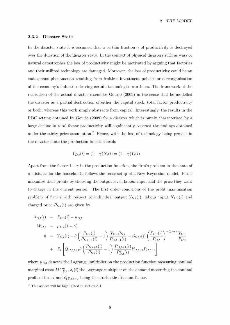
2.3.2 Disaster State
In the disaster state it is assumed that a certain fraction γ of productivity is destroyed
over the duration of the disaster state. In the context of physical disasters such as wars or
natural catastrophes the loss of productivity might be motivated by arguing that factories
and their utilized technology are damaged. Moreover, the loss of productivity could be an
endogenous phenomenon resulting from fruitless investment policies or a reorganisation
of the economy’s industries leaving certain technologies worthless. The framework of the
realisation of the actual disaster resembles Gourio (2009) in the sense that he modelled
the disaster as a partial destruction of either the capital stock, total factor productivity
or both, whereas this work simply abstracts from capital. Interestingly, the results in the
RBC setting obtained by Gourio (2009) for a disaster which is purely characterised by a
large decline in total factor productivity will significantly contrast the findings obtained
under the sticky price assumption.7 Hence, with the loss of technology being present in
the disaster state the production function reads
YD,t(i) = (1− γ)Nt(i) = (1− γ)Yt(i)
Apart from the factor 1− γ in the production function, the firm’s problem in the state of
a crisis, as for the households, follows the basic setup of a New Keynesian model. Firms
maximise their profits by choosing the output level, labour input and the price they want
to charge in the current period. The first order conditions of the profit maximisation
problem of firm i with respect to individual output YD,t(i), labour input ND,t(i) and
charged price PD,t(i) are given by
λD,t(i) = PD,t(i)− µD,t
WD,t = µD,t(1− γ)
0 = YD,t(i)− θ(
PD,t(i)
PD,t−1(i)− 1
)YD,tPD,tPD,t−1(i)
− ελD,t(i)(PD,t(i)
PD,t
)−(1+ε) YD,tPD,t
+ Et
[QD,t,t+1θ
(PD,t+1(i)
PD,t(i)− 1
)PD,t+1(i)
P 2D,t(i)
YD,t+1PD,t+1
]
where µD,t denotes the Lagrange multiplier on the production function measuring nominal
marginal costs MCnD,t, λt(i) the Lagrange multiplier on the demand measuring the nominal
profit of firm i and QD,t,t+1 being the stochastic discount factor.
7 This aspect will be highlighted in section 3.4.
8
2 THE MODEL
2.3.3 Normal Times
Obviously, in normal times there is no current loss or destruction of productivity, but firms
operate in their usual setting with the linear production function presented in the general
setting of the firms. This in turn causes an immediate but minor alteration in one of the
firm’s first order conditions, namely the one obtained from the differentiation of the profit
function with respect to labour input Nt(i), which in normal times simply reads
Wt = µt
with µt again denoting the Lagrange multiplier on the production function measuring
nominal marginal costs MCnt in normal times.
The dominant change on the firm’s side of the economylies in the first order condition
with respect to one’s chosen price Pt(i) as it features an expected value. By forming
expectations about variables in t+ 1 the firm needs to assign a probability or weight of ψt
to the disaster state and a weight of 1− ψt to the scenario in which the economy remains
in normal times. Hence, as brought up in the intertemporal Euler equation, the expected
value needs to be split up yielding the following first order condition for Pt(i) for the
normal times state
0 = Yt(i)− θ(
Pt(i)
Pt−1(i)− 1
)YtPtPt−1(i)
− ελt(i)(Pt(i)
Pt
)−(1+ε) YtPt
+ ψtEt
[Qt,D,t+1θ
(PD,t+1(i)
Pt(i)− 1
)PD,t+1(i)
P 2t (i)
YD,t+1PD,t+1
]+ (1− ψt)Et
[Qt,t+1θ
(Pt+1(i)
Pt(i)− 1
)Pt+1(i)
P 2t (i)
Yt+1Pt+1
]This rather unpleasant looking optimality condition appears to be challenging to analyse.
So far, it does not deliver a clear image of how a shock on ψt transmits through the supply
side of the economy and whether firms will increase or decrease their prices in response to
an increase in ψt. However, the discussion on optimal monetary policy will deliver a strong
simplification resulting in a convenient log-linearised version of the optimality condition
stated above.
2.4 Monetary Authority
To close the setup of the theoretical model, this section deals with the monetary authority
operating in the previously described economy. It is convenient to firstly consider optimal
9

2 THE MODEL
monetary policy in the transition period when the economy jumps from the normal times
state into the disaster state and its implications for the inflation rate in the transition
PD,t+1
Pt. From the perspective of normal times it is known that agents anticipate a sharp
drop in output, and hence consumption, if a disaster truly realises, where this negative
outlook might cause agents to extremely react to changes in ψt by the intertemporal
Euler equation as a matter of risk aversion or simply anxiety about the future. These
overreactions should not be in the general interest of the monetary authority. Rather one
could think about a monetary authority trying to let the disaster scenario appear less
disastrous in order to ease agent’s expectations about the future. Such a relaxation of
facts is expected to happen when the monetary authority commits to a policy in which
they allow for a relatively high transition inflation ratePD,t+1
Pt. As consumption in the
disaster state will be only a fraction of the normal times consumption level, marginal
utility of consumption in the disaster state will be very high such that, in order to smooth
the relation of consumption at time t + 1 in the two distinct states of nature, the real
return on borrowing or lending should be low when the crisis hits.
From the perspective of normal times, such inflationary promises in the state of transition
seem to be desirable but it remains questionable whether such a policy is time-consistent
or subject to re-optimisation at another point in time. Considering the actual realisation
of the disaster, and hence the transition period, the inflationary promises do not appear
to be a policy the monetary authority will undoubtedly stick to. Due to its deterministic
design the monetary authority has the ability to implement the flexible price allocation
in the disaster state and allowing for a high transition inflation would solely create a high
degree of distortion in the economy. As a consequence, it seems to be more reasonable
to think that monetary policy will be re-optimised in the transition period in order to
eliminate any distortion arising from its inflation rate, namely to setPD,t+1
Ptequal to 1.
This assumption of a discretionary monetary policy in the transition when the disaster
actually hits causes a strong simplification of the first order conditions of the households
and the firms. By log-linearisation around a zero-inflation and symmetric steady state one
obtains the two New Keynesian Phillips Curves (NKPC) which read
πD,t−1,t = βEtπD,t,t+1 +ε− 1
θ(σ + κ)yD,t and πt−1,t = (1− ψ)βEtπt,t+1 +
ε− 1
θ(σ + κ)yt
where ψ denotes the steady state level of the disaster probability. The similarity and
standard character of the two NKPCs for the two states of nature are a practical feature
for choosing an appropriate form of monetary policy. By following a Taylor (1993) rule,
10

2 THE MODEL
usually expressed as
it = φππt−1,t + φyyt and iD,t = φππD,t−1,t + φyyD,t
the monetary authority can ensure local determinacy by restricting the values of φy and
φπ, which denote the preferences of the monetary authority in terms of inflation and out-
put stabilisation.8 In conclusion, it is assumed that the monetary authority follows a
Taylor (1993) rule in both states of nature, while in the transition from normal times to
the state of disaster she is assumed to deviate from this commitment in order to limit the
distortion arising from the transition inflation as discussed in the foregoing paragraphs.9
2.5 Equilibrium
Concerning both states in which the economy exists, as used in the determination of
optimal monetary policy, this paper focuses on symmetric equilibria, that is all firms
charge the same price such that Pt(i) = Pt and hire the same amount of labour. Since all
households are assumed to be identical the market clearing condition for the credit market
is
Bt = 0 ∀t
that is borrowing or lending has to be balanced on aggregate. In order to clear the goods
market it has to hold in both states of nature that
Ct(i) = Yt(i)
which in turn implies
Ct = Yt
In other words, all produced output is consumed by the households. Moreover, the third
market clearing condition considers the labour market where optimality requires that
Nt =
∫ 1
0Nt(i)di
8 See, for example, Gali and Gertler (1999) for a discussion of advantages and shortcomings arising from
preferences of the monetary authority.9 The concrete form of this discretionary policy is not derived in this paper as only its result that
PD,t+1
Pt= 1
is needed for the solution of the model.
11
3 RESULTS
Lastly, in equilibrium the nominal interest rate needs to be non-negative,
it ≥ 0
for otherwise households would benefit from arbitrage opportunities.
Combining these statements with the optimality conditions of the households and firms
derived in the previous subsections and the lastly found simplification ofPD,t+1
Pt= 1 delivers
a parsimonious set of equilibrium conditions which after log-linearisation around the zero-
inflation steady state, in which it holds that CD = (1− γ)C, read
πD,t−1,t =ε− 1
θ(σ + κ)yD,t + βEtπD,t,t+1 (1)
yD,t = EtyD,t+1 −1
σ(iD,t − EtπD,t,t+1) (2)
iD,t = φππD,t−1,t + φyyD,t (3)
πt−1,t =ε− 1
θ(σ + κ)yt + (1− ψ)βEtπt,t+1 (4)
−σyt = −σψβ(1 + i)(1− γ)−σEtyD,t+1
− σ(1− ψ)β(1 + i)Etyt+1
+ it − (1− ψ)β(1 + i)Etπt,t+1
+ [β(1− γ)−σ(1 + i)− β(1 + i)]ψψt
(5)
it = φππt−1,t + φyyt (6)
The first three equations characterise the disaster state by a very basic setup of a standard
New Keynesian model, while the last three equations capture the economy in normal
times. While equation 4, the NKPC in normal times, does not largely differ from its
disaster counterpart in equation 1, it is evident that the log-linearised Euler equation, or
New Keynesian IS curve, in normal times displayed by equation 5 heavily differs from its
standard representation as in equation 2 as it also features the disaster variable yD,t+1 as
well as it is directly affected by percentage deviations of the disaster probability from its
steady state ψt.
3 Results
This section deals with the results of shocks on the disaster probability in the New Key-
nesian model graphically illustrated by impulse response functions. The subsequent para-
graphs present a baseline calibration of the model with which the first results are obtained
12

3 RESULTS
Parameter Symbol Value
Relative risk aversion (inverse of intertemp. elasticity) σ 1
Frisch elasticity of labour supply 1/κ 1
Steady state nominal interest rate i 0.01
Price elasticity of demand ε 11
Discount factor β 0.9869
Steady state disaster probability ψ 0.00425
Size of output destruction γ 0.43
Rotemberg parameter θ 116.51
Persistence of AR(1) ρ 0.9
Weight on inflation stabilisation in Taylor rule φπ 1.5
Weight on output stabilisation in Taylor rule φy 0.125
Table 1: Calibration of parameter values for the baseline model
and displayed. Furthermore, a sensitivity analysis with respect to the nominal rigidity is
executed in order to motivate a following critical reception on the disaster hypothesis.
3.1 Calibration
Parameters and their calibration are listed in Table 1 where one period is set to be one
quarter. To account for disagreements on parameter values for σ and κ in the existing
literature the assumption of log-utility and a unit Frisch elasticity of labour supply is con-
sidered as an acceptable compromise for a baseline calibration. In the appendix, different
parameter values are considered serving as a robustness check of the results obtained from
the baseline calibration.
Crucial elements such as the steady state value for the probability of entering a state of
disaster ψ follows the empirical finding of 1.7% per year by Barro (2006), and hence 0.4%
per quarter,as well as the baseline size for the destruction rate of 43% in a disaster which
has also been used in Gourio (2009). As shown in the setup of the model, the inclusion of
the disaster state significantly alters the intertemporal Euler equation and consequently
the determination of certain parameters. In the steady state the intertemporal Euler
equation reads
(1 + i) =1
β
1
ψ(1− γ)−σ + (1− ψ)
revealing a slight restriction of the model regarding its calibration. By fixing specific
parameter values one variable has to be chosen which will be determined endogenously.
As this paper seeks to assign the stated values for γ and ψ found by Barro (2006) either i
13
3 RESULTS
or β needs to be determined endogenously. In order to avoid possible negative values of i
which would arise for certain parameter combinations by fixing the value of β, this paper
takes a commonly assumed value for the steady state annual real return of 4% by allowing
β to vary with parameter variations.10
The evolution of percentage deviations of the disaster probability from its steady state
value is modelled as an AR(1) process, i.e.
ψt = ρψt−1 + ξt
with ρ measuring the persistence, being calibrated to a value of 0.9, and ξt denoting the
stochastic innovation.
As arguably troublesome to calibrate stands the Rotemberg parameter θ as it does not
feature an empirical counterpart, as an average contract length or lifetime of a price,
allowing the measurement of appropriate values. This deficiency has been addressed by
Keen and Wang (2007) who show a convenient and intuitive way to express θ by β, ε and
the Calvo parameter α measuring the average lifetime of a price by 1/(1 − α).11 As a
baseline value it is assumed that on average firms change or adjust their prices once a year
or every four quarters as found by Rotemberg and Woodford (1995), which designates a
value of 116.51 for θ. Due to general disagreements in the literature on the strength of
price stickiness in general or on an industry-specific level, the sensitivity analysis discusses
variations of θ as well as the flexible price scenario in which θ is equal to zero.
Lastly, Table 1 lists the parameters of the Taylor rule φπ and φy. The chosen calibration
lies in a standard range being in line with Christiano et al. (2005) and Keen and Pakko
(2011), emphasising the focus on inflation stabilisation via φπ rather than responses of the
interest rate to output deviations by φy. Since this paper’s focus does not lie on the analysis
of monetary policy, variations in the last two mentioned parameters will not be explicitly
discussed in the following. However, and for the sake of completeness, a sensitivity analysis
of impulse responses for different combinations of φπ and φy is displayed in Figure 6 in
appendix A.
10As a side note, as γ → 0 or ψ → 0 one obtains the usual relation of 1 + i = 1/β which would imply the
usually taken value of 0.99 for β.11The formula stated by Keen and Wang (2007) to determine θ by observables reads θ = [(ε−1)α]
[(1−α)(1−βα)] .
14

3 RESULTS
3.2 Response to an Increase in the Disaster Probability
After declaring the baseline calibration, the key exercise of this paper, to exogenously
increase the probability of a disaster, is performed, where it is assumed that the probability
of entering a disaster doubles at time t = 0 from 0.425% to 0.85% per quarter. Figure 1
displays the impulse responses of output, the nominal interest rate, and inflation rate.12
Output decreases and initially falls to approximately 0.3% below its steady state level
accompanied with a drop in the price level displayed by negative inflation in the center
panel. According to the Taylor principle the nominal interest rate drops as both output and
inflation are below their steady state levels. Geometrically declining with the persistence
parameter of the probability process all series move back to their steady state. Emphasis
0 10 20 30
0.4
0.5
0.6
0.7
0.8
0.9
1
in %
poin
ts
Nominal interest rate
quarters0 10 20 30
−0.4
−0.3
−0.2
−0.1
0
quarters
Inflation rate
in %
poin
ts
0 10 20 30
−0.3
−0.2
−0.1
0
% d
evia
tion fro
m s
teady s
tate
Output
quarters
Figure 1: The effect on an increase in the disaster probability. Displayed are the impulse
responses for the baseline calibration where at t = 0 the disaster probability doubles from 0.425%
to 0.85% per quarter. The red line denotes the steady state.
has to be put on the fact that these impulse responses reveal that an arguably small
increase in the chance to enter a disaster to 0.85% per quarter leads to a recession in the
economy.
As the disaster state becomes more probable, or agents become more pessimistic, they have
a higher incentive to save in pursuance of insuring themselves against the higher perceived
risk in the economy. The only tool of saving in the economy, borrowing or lending, is
12Due to the simplistic setup of the model it holds that yt = ct = nt and hence it is appropriate to solely
report output responses.
15

3 RESULTS
constrained to be zero on aggregate, which leaves agents with no other choice than to
reduce current consumption, and by market clearing output as well as labour input, in
order to smooth out a possible huge drop in consumption if the disaster would actually
realise. The drop in demand faced by the firms gives rise to price lowering motives causing
the drop in the price level and hence deflation of around 0.4%. As the nominal interest
rate responds to both outlined deviations it comes very close to the zero lower bound as
to be seen in the initial shock period, where the level of the nominal interest rate drops
to 0.33%. As the shock on ψt has only been temporary the monetary authority does not
face an actual liquidity trap, but it is recognisable that parameter alterations might easily
cause the impotence of monetary policy when the zero lower bound becomes binding.
To summarise, all presented responses are the result of a disputable small increase in the
disaster probability to 0.85% per quarter. Especially the reaction of output appears to be
quite significant for this slight increase in agent’s perceived risk or pessimism towards the
future. On the contrary, the deflation rate following the increase in the disaster probability
appears to be reasonably small keeping in mind that the model is based on a zero-inflation
steady state.
In the following, parameter variations in θ will be considered, determining the sensitivity
of the previously presented results with respect to the nominal rigidity. 13
3.3 Robustness with Respect to θ
The basic calibration of θ implied an average lifetime of a price of a year or 4 quarters,
which denotes quite a solid degree of stickiness in the economy. The considerations in this
paragraph are twofold as θ will be calibrated to values implying average price lifetimes of
2 and 5 quarters as well as the flexible price benchmark economy attained by setting θ
equal to zero.14 Figure 2 displays the impulse responses to a 10% increase in the disaster
probability for the different calibrations of θ where the red line, denoting the steady state,
coincides with the response of output in the flexible price benchmark economy (dashed
line).15
13For sensitivity checks of σ, κ, φπ, φy and γ please see appendix A.14 In these alterations the steady state markup remains fixed to 10%.15An unpleasant by-product with the initially used size of the shock, i.e. a 100% increase of the disaster
probability, and higher values of θ the monetary authority hits the zero lower bound, that is has to set
the nominal interest rate to zero. To allow for a comparable graphical illustration the size of the shock
has been reduced to a 10% increase in the disaster probability.
16

3 RESULTS
0 10 20 300.92
0.94
0.96
0.98
1in
% p
oin
tsNominal interest rate
quarters0 10 20 30
−0.05
−0.03
−0.01
0
quarters
Inflation rate
in %
poin
ts
0 10 20 30−0.05
−0.03
−0.01
0
% d
evia
tion fro
m s
teady s
tate
Output
quarters
Figure 2: Sensitivity of impulse responses with respect to θ. Impulse responses to a 10%
increase in the probability of a disaster in t = 0 for θ = 0 (dashed), θ = 19.80 (dotted), θ = 116.51
(solid) and θ = 192.31 (dotdashed). The red line denotes the steady state.
Generally, it can be said that with a rising strength of the nominal rigidity, the decline
in output below its steady state level amplifies while the responses of inflation and the
nominal interest rate are dampened. With a rigidity implying an average price lifetime
of 5 quarters (θ = 192.31) placing a 10% increase in the probability of a disaster causes
a decline in output of more than 0.04% below its steady state level. Concerning the
flexible price benchmark economy, where θ equals zero, it is apparent that there are no
real effects in the economy as the probability of a future disaster increases. The shock
entirely transmits through inflation and the nominal interest rate.
In conclusion it can be said that variations in θ drive the relative transmission of shocks on
the disaster probability. As the degree of price stickiness increases the effects of the shock
are carried out by the real economy while in a flexible price economy the real economy
stays unaffected and solely the nominal interest rate and inflation rate respond.
3.4 The Barro-Rietz Hypothesis in a DSGE framework
The foregoing sensitivity check revealed that the sign of the responses to an increase in
the disaster probability is robust to variations in the parameter calibration, while the
magnitude as well as the relative responses of nominal and real variables are subject to
parameter values. After achieving these results, it is interesting to compare the sign of the
17

3 RESULTS
obtained responses in the sticky price model of this paper to the ones obtained by Gourio
(2009) in the RBC setting. As mentioned earlier, he considers three possible disaster
scenarios being characterised by either a large destruction of the capital stock, total factor
productivity, or both. By considering the disaster scenario in which, as well as in this
work, total factor productivity is destroyed he finds the reverse response of output, that
is an increase in the probability of the disaster leads to a boom in the economy. On the
other hand, by inspecting the disaster scenarios in which a certain fraction of the capital
stock is erased he finds the negative response of output identical to the response displayed
in the antecedent paragraphs of this section. In order to correct the sign of the response
of output and match key business cycle statistics he needed to add large adjustment costs
to the disaster scenario of pure productivity destruction.
Naturally, this difference in the response of output stems from the involvement of capital
accumulation in his model. When the disaster is assumed to not affect the capital stock,
investments in this stock denote a device of saving and insurance against the disaster
state. Consequently, agents increase investments due to a precautionary savings motive
in response to an increase in the disaster probability causing a rise in the stock of capital
and hence an increase in aggregate production explaining the reverse response of output
in the RBC setting. Moreover, the abstraction from capital in this work puts emphasis on
uninsured intertemporal smoothing as the increase in the disaster probability represents a
negative wealth effect. Due to its simplistic design output, consumption and hours worked
perfectly comove, while in Gourio (2009) the sign of the consumption response opposes
the one of the other two when considering a disaster scenario with capital destruction.
This denotes a small success of the sticky price model with the disaster hypothesis since
it does not fail to generate a positive comovement of consumption and hours worked.
Finally, this paper shows that by removing the nominal rigidity (θ = 0) alterations in the
disaster probability transmit through nominal variables alone leaving the real economy
unaffected, which highlights the importance of including capital in the RBC context in
order to achieve success.
This comment on the different results of the disaster hypothesis by adapting particular
modelling assumptions gives rise to a critical reception on the inclusion of the Barro-Rietz
hypothesis in DSGE models. To begin with, in the review of the literature it became
apparent that there exist numerous definitions and hence approaches to model the disaster
hypothesis. In the foregoing comparison to the RBC setting this paper revealed that
18

4 CONCLUSION
depending on the general setup of the model one can obtain reverse responses of variables
which are of interest. As there does not exist a unified picture on how to model or
implement the disaster state in macroeconomic models one should question the validity of
the hypothesis’ success in explaining phenomena in macroeconomics in general, specifically
in the area of macro-finance. By combining different modelling assumptions the disaster
hypothesis can be designed to be successful, which has been a common approach in the
disaster literature illustrating a way of residualisation of the disaster aspect. Movements
or variances of the disaster probability were set or backed out from model frameworks
in order to optimally match phenomena or puzzles in macro-finance, where the critical
examination of obtained disaster probability aspects as the size, time series behaviour, and
the definition itself mostly fails to appear. Secondly, and more obviously, the difficulty to
empirically assess the disaster probability and its movements continues to hinder the full
acceptance of the Barro-Rietz hypothesis. The model considered in this paper comes with
the deficiency that the tiniest movements in the disaster probability cause the zero lower
bound to bind, which was the reason for the reduced size of the shock on the disaster
probability in the sensitivity analysis. In order to appropriately judge and evaluate this
theoretical drawback as well as to justify the quantitative assumptions which have been
made on the Barro-Rietz hypothesis in the macro-finance literature, future focus has to be
put on a convenient and convincing empirical assessment most favourably detached from
theoretical containments.
4 Conclusion
This work shows that exogenous variations in the probability for a future disaster in a
New Keynesian model causes significant responses of real and nominal variables. Most
importantly the model suggests that an increase in the aggregate risk perceived by house-
holds and firms leads to a recession in the economy which stands in line with findings of
Gourio (2009) in the context of an RBC model. The replication of this finding depends
heavily on the definition of the disaster state and the limited saving opportunities of the
households inasmuch as the presented model abstracts from capital accumulation. On that
account, this work questions the validity and the success of the Barro-Rietz hypothesis
in DSGE models believing that there exist several aspects which need to be adressed in
future research.
To begin with, and in order to avoid the common approach of residualising the disaster
19

4 CONCLUSION
hypothesis, it would be interesting to find further empirical support, specifically quantify-
ing movements in the disaster probability. Since these are captured in agents’ optimism
or pessimism towards the future they might be extractable from, for example, business
outlook surveys. By feeding these into a theoretical framework one could validate the
success of the Barro-Rietz assumption.
Furthermore, while earthquakes or hurricanes certainly denote exogenous events it is more
likely that for instance financial crises indicate an endogenous phenomenon in the econ-
omy. Accordingly, it would be interesting to endogenise variations in the probability for a
disaster as well as its realisation allowing for economic crashes which have been induced by
agents’ behaviour. In light of this aspect, future research could consider the Barro-Rietz
assumption in models of heterogeneous agents concerning the degree of individual risk
aversion in which the decisions of a small fraction of the population can significantly drive
the disaster probability.
20
REFERENCES
References
Barro, R. J. (2005): “Rare Events and the Equity Premium,” Working Paper 11310,
National Bureau of Economic Research.
——— (2006): “Rare Disasters and Asset Markets in the Twentieth Century,” The Quar-
terly Journal of Economics, 121, pp. 823–866.
Blanchard, O. and J. Gali (2007): “Real Wage Rigidities and the New Keynesian
Model,” Journal of Money, Credit and Banking, 39, 35–65.
Blundell, R. and T. Macurdy (1999): Labor Supply: A Review of Alternative Ap-
proaches., U College London and Institute for Fiscal Studies: Handbooks in Economics,
vol. 5., 1559 – 1695.
Calvo, G. A. (1983): “Staggered prices in a utility-maximizing framework,” Journal of
Monetary Economics, 12, 383 – 398.
Christiano, L. J., M. Eichenbaum, and C. L. Evans (2005): “Nominal Rigidities
and the Dynamic Effects of a Shock to Monetary Policy,” Journal of Political Economy,
113, pp. 1–45.
Dixit, A. K. and J. E. Stiglitz (2000): Monopolistic Competition and Optimum Prod-
uct Diversity., Princeton U: Readings for Contemporary Economics., 126 – 144.
Eichenbaum, M. and J. D. M. Fisher (2007): “Estimating the Frequency of Price
Re-optimization in Calvo-Style Models.” Journal of Monetary Economics, 54, 2032 –
2047.
Farhi, E. and X. Gabaix (2008): “Rare Disasters and Exchange Rates,” Working Paper
13805, National Bureau of Economic Research.
Gabaix, X. (2008): “Variable Rare Disasters: A Tractable Theory of Ten Puzzles in
Macro-finance.” American Economic Review, 98, 64 – 67.
Gali, J. (2002): “New Perspectives on Monetary Policy, Inflation, and the Business
Cycle,” NBER Working Papers 8767, National Bureau of Economic Research, Inc.
Gali, J. and M. Gertler (1999): “Inflation dynamics: A structural econometric anal-
ysis,” Journal of Monetary Economics, 44, 195 – 222.
21

REFERENCES
Gourio, F. (2008a): “Disasters and Recoveries.” American Economic Review, 98, 68 –
73.
——— (2008b): “Time-series predictability in the disaster model,” Boston University -
Department of Economics - Working Papers Series wp2008-016, Boston University -
Department of Economics.
——— (2009): “Disasters Risk and Business Cycles,” Working Paper 15399, National
Bureau of Economic Research.
Hall, R. E. (1988): “Intertemporal Substitution in Consumption,” Journal of Political
Economy, 96, 339–57.
Keen, B. and Y. Wang (2007): “What is a realistic value for price adjustment costs in
New Keynesian models?” Applied Economics Letters, 14, 789–793.
Keen, B. D. and M. R. Pakko (2011): “Monetary Policy and Natural Disasters in a
DSGE Model.” Southern Economic Journal, 77, 973 – 990.
Kehoe, T. J. and e. Prescott, Edward C. (2007): Great Depressions of the Twentieth
Century., Federal Reserve Bank of Minneapolis.
Maddison, A. (2003): The World Economy: Historical Statistics, Paris: OECD.
Mankiw, N. G. (1985): “Small Menu Costs and Large Business Cycles: A Macroeconomic
Model of Monopoly,” The Quarterly Journal of Economics, 100, pp. 529–537.
Mehra, R. and E. C. Prescott (1985): “The equity premium: A puzzle,” Journal of
Monetary Economics, 15, 145 – 161.
Nakamura, E., J. Steinsson, R. Barro, and J. Ursa (2010): “Crises and Recoveries
in an Empirical Model of Consumption Disasters,” Working Paper 15920, National
Bureau of Economic Research.
Niemann, S. and P. Pichler (2011): “Optimal Fiscal and Monetary Policies in the
Face of Rare Disasters.” European Economic Review, 55, 75 – 92.
Rietz, T. A. (1988): “The Equity Risk Premium: A Solution.” Journal of Monetary
Economics, 22, 117 – 131.
Rotemberg, J. J. (1982): “Sticky Prices in the United States,” Journal of Political
Economy, 90, pp. 1187–1211.
22

REFERENCES
Rotemberg, J. J. and M. Woodford (1995): Oligopolistic Pricing and the Effects of
Aggregate Demand on Economic Activity., MIT: Elgar Reference Collection. Interna-
tional Library of Critical Writings in Economics, vol. 58., 418 – 472.
Schmitt-Grohe, S. and M. Uribe (2004): “Optimal Fiscal and Monetary Policy under
Sticky Prices.” Journal of Economic Theory, 114, 198 – 230.
——— (2010): “Chapter 13 - The Optimal Rate of Inflation,” Elsevier, vol. 3 of Handbook
of Monetary Economics, 653 – 722.
Taylor, J. B. (1980): “Aggregate Dynamics and Staggered Contracts,” Journal of Po-
litical Economy, 88, pp. 1–23.
——— (1993): “Discretion versus Policy Rules in Practice.” Carnegie-Rochester Confer-
ence Series on Public Policy, 39, 195 – 214.
Wachter, J. (2008): “Can Time-Varying Risk of Rare Disasters Explain Aggregate Stock
Market Volatility?” Working Paper 14386, National Bureau of Economic Research.
Woodford, M. (2003): Interest and prices., Princeton and Oxford:.
23

A FIGURES
A Figures
0 10 20 30−0.1
0
0.1
0.2
0.3
0.4
0.5
0.6
0.7
0.8
0.9
in %
poin
ts
Nominal interest rate
quarters0 10 20 30
−0.4
−0.2
0
−0.6
quarters
Inflation rate
in %
poin
ts
0 10 20 30
−0.2
−0.1
0
% d
evia
tion fro
m s
teady s
tate
Output
quarters
Figure 3: Sensitivity of impulse responses with respect to σ. Impulse responses to a 10%
increase in the probability of a disaster in t = 0 for σ = 1 (solid), σ = 3 (dotted) and σ = 5
(dotdashed). The red line denotes the steady state.
24

A FIGURES
0 10 20 300.92
0.94
0.96
0.98
1
in %
poin
ts
Nominal interest rate
quarters0 10 20 30
−0.05
−0.03
−0.01
0
quarters
Inflation rate
in %
poin
ts
0 10 20 30−0.03
−0.02
−0.01
0
% d
evia
tion fro
m s
teady s
tate
Output
quarters
Figure 4: Sensitivity of impulse responses with respect to κ. Impulse responses to a 10%
increase in the probability of a disaster in t = 0 for κ = 1 (solid), κ = 3 (dotted) and κ = 5
(dotdashed). The red line denotes the steady state.
0 10 20 300.85
0.9
0.95
1
in %
poin
ts
Nominal interest rate
quarters0 10 20 30
−0.09
−0.07
−0.05
−0.03
−0.01
0
quarters
Inflation rate
in %
poin
ts
0 10 20 30
−0.05
−0.03
−0.01
0
% d
evia
tion fro
m s
teady s
tate
Output
quarters
Figure 5: Sensitivity of impulse responses with respect to γ. Impulse responses to a 10%
increase in the probability of a disaster in t = 0 for γ = 0 (dashed), γ = 0.1 (dotted), γ = 0.43
(solid) and γ = 0.6 (dotdashed). The red line denotes the steady state.
25

A FIGURES
0 10 20 300.92
0.94
0.96
0.98
1
in %
poin
ts
Nominal interest rate
quarters0 10 20 30
−0.05
−0.03
−0.01
0
quarters
Inflation rate
in %
poin
ts
0 10 20 30
−0.03
−0.01
0
% d
evia
tion fro
m s
teady s
tate
Output
quarters
Figure 6: Sensitivity of impulse responses with respect to φπ and φy. Impulse responses to
a 10% increase in the probability of a disaster in t = 0 for pairs of (φπ, φy) of (1.5, 0.125) (solid),
(1.5, 0) (dotted), (5, 0) (dotdashed) and (5, 1) (dashed). The red line denotes the steady state.
26
SFB 649 Discussion Paper Series 2013
For a complete list of Discussion Papers published by the SFB 649, please visit http://sfb649.wiwi.hu-berlin.de. 001 "Functional Data Analysis of Generalized Quantile Regressions" by
Mengmeng Guo, Lhan Zhou, Jianhua Z. Huang and Wolfgang Karl Härdle, January 2013.
002 "Statistical properties and stability of ratings in a subset of US firms" by Alexander B. Matthies, January 2013.
003 "Empirical Research on Corporate Credit-Ratings: A Literature Review" by Alexander B. Matthies, January 2013.
004 "Preference for Randomization: Empirical and Experimental Evidence" by Nadja Dwenger, Dorothea Kübler and Georg Weizsäcker, January 2013.
005 "Pricing Rainfall Derivatives at the CME" by Brenda López Cabrera, Martin Odening and Matthias Ritter, January 2013.
006 "Inference for Multi-Dimensional High-Frequency Data: Equivalence of Methods, Central Limit Theorems, and an Application to Conditional Independence Testing" by Markus Bibinger and Per A. Mykland, January 2013.
007 "Crossing Network versus Dealer Market: Unique Equilibrium in the Allocation of Order Flow" by Jutta Dönges, Frank Heinemann and Tijmen R. Daniëls, January 2013.
008 "Forecasting systemic impact in financial networks" by Nikolaus Hautsch, Julia Schaumburg and Melanie Schienle, January 2013.
009 "‘I'll do it by myself as I knew it all along’: On the failure of hindsight-biased principals to delegate optimally" by David Danz, Frank Hüber, Dorothea Kübler, Lydia Mechtenberg and Julia Schmid, January 2013.
010 "Composite Quantile Regression for the Single-Index Model" by Yan Fan, Wolfgang Karl Härdle, Weining Wang and Lixing Zhu, February 2013.
011 "The Real Consequences of Financial Stress" by Stefan Mittnik and Willi Semmler, February 2013.
012 "Are There Bubbles in the Sterling-dollar Exchange Rate? New Evidence from Sequential ADF Tests" by Timo Bettendorf and Wenjuan Chen, February 2013.
013 "A Transfer Mechanism for a Monetary Union" by Philipp Engler and Simon Voigts, March 2013.
014 "Do High-Frequency Data Improve High-Dimensional Portfolio Allocations?" by Nikolaus Hautsch, Lada M. Kyj and Peter Malec, March 2013.
015 "Cyclical Variation in Labor Hours and Productivity Using the ATUS" by Michael C. Burda, Daniel S. Hamermesh and Jay Stewart, March 2013.
016 "Quantitative forward guidance and the predictability of monetary policy – A wavelet based jump detection approach –" by Lars Winkelmann, April 2013.
017 "Estimating the Quadratic Covariation Matrix from Noisy Observations: Local Method of Moments and Efficiency" by Markus Bibinger, Nikolaus Hautsch, Peter Malec and Markus Reiss, April 2013.
018 "Fair re-valuation of wine as an investment" by Fabian Y.R.P. Bocart and Christian M. Hafner, April 2013.
019 "The European Debt Crisis: How did we get into this mess? How can we get out of it?" by Michael C. Burda, April 2013.
SFB 649, Spandauer Straße 1, D-10178 Berlin http://sfb649.wiwi.hu-berlin.de
This research was supported by the Deutsche
Forschungsgemeinschaft through the SFB 649 "Economic Risk".
SFB 649, Spandauer Straße 1, D-10178 Berlin http://sfb649.wiwi.hu-berlin.de
This research was supported by the Deutsche
Forschungsgemeinschaft through the SFB 649 "Economic Risk".
SFB 649 Discussion Paper Series 2013
For a complete list of Discussion Papers published by the SFB 649, please visit http://sfb649.wiwi.hu-berlin.de. 020 "Disaster Risk in a New Keynesian Model" by Maren Brede, April 2013.