Embed Size (px)
Citation preview

DIRECTIONAL MEASUREMENTS AND MODELLING OF INDOOR ENVIRONMENTS AT 5.2GHZ
D.I. Laurenson*, C.M. Tan†, C.C. Chong* and M.A. Beach† *Institute for Digital Communications, School of Engineering and Electronics
The University of Edinburgh, Mayfield Road, Edinburgh, U.K., EH9 3JL †Centre for Communication Research, Electrical Engineering
University of Bristol, Bristol, U.K. phone: + (44) 131 650 5579, fax: + (44) 131 650 6554, email: [email protected]
phone: + (44) 117 954 5190, fax: + (44), email: [email protected] web: www.mobilevce.com
ABSTRACT State of the art antenna array systems require detailed infor-mation about the channel in order to maximise usable capac-ity. Such systems require both detailed analysis and realistic simulation based testing. To date there has been little work carried out in the area of directional channel characterisation when one of the terminals is in motion. This paper will de-scribe a dynamic measurement campaign, conducted at Bris-tol University, employing antenna arrays, both for a SIMO configuration with a ULA, and a MIMO configuration em-ploying CUBAs. Associated with the SIMO measurements, a modelling strategy was developed for simulating direc-tional multipath propagation. The model is based on sto-chastic processes controlling the birth and death of observ-able multipath components, the temporal and spatial correla-tion of multipath components, the variation of the spatial and temporal properties of components as the terminal moves, and the spectral characteristics of these components. The generic framework is fitted to the measurements ob-tained, and the resulting parameters are presented.
1. INTRODUCTION
Radio channel measurement and modelling have been key elements in the assessment of communication systems since the first hardware simulators appeared. They are no less important today, although the systems that they support are infinitely more complex than those produced decades ago. Currently, the research focus is on directional channel mod-els that may or may not incorporate the dynamic evolution of the environment. Such models are essential for assessing the potential of smart antenna based systems – key elements for support of high bandwidth communication.
In recent years, many studies have been conducted in order to gain a more detailed knowledge of radio propaga-tion. Numerous channel models have been reported in the literature [1], [2]. A major shortcoming of many of these is that they do not consider dynamic behaviour of the channels, concentrating instead on a statistically stationary description of the channel. This can be attributed to the lack of dynamic measurement campaigns to support realistic modelling of a dynamic channel.
This paper describes work that has been carried out by Bristol University and The University of Edinburgh in the UK under the auspices of the Virtual Centre of Excellence in Mobile Communications (MobileVCE). Channel measure-ments were conducted by Bristol University, encompassing both dynamic SIMO and dynamic MIMO measurements, while the channel modelling work was carried out at The University of Edinburgh, principally focussing on the Dy-namic SIMO data. Work to extend the model to the dynamic MIMO case is currently underway.
The remainder of the paper is organised as follows: Sec-tion 2 will describe the measurement equipment and opera-tion, and section 3 the key parameters extracted from these measurements. Section 4 will introduce the modelling work, while section 5 will draw the paper to a close.
2. CHANNEL MEASUREMENTS
2.1 Measurement setup Two sets of measurements were obtained for channel
modelling purposes, a set of single input multiple output (SIMO) measurements, and a set of multiple input multiple output (MIMO) measurements. Both sets were conducted using a Medav RUSK BRI channel sounder operating at 5.2 GHz [3]. A periodic multitone signal with a bandwidth of 120 MHz and repetition period of 0.8 µs was used. The fre-quency domain channel response was calculated online and stored on the sounder’s hard disk for post-processing.
For the SIMO measurements, the mobile transmitter (TX) used an omni-directional antenna transmitting at an input power of +26 dBm with a stationary receiver (RX) comprising a uniform linear array (ULA). The ULA had 8 active dipole-like elements spaced by half a wavelength and 2 dummy elements at both ends to balance the mutual cou-pling effects. The effective azimuth visible range of the ULA was 120º.
For the MIMO measurements, two identical 16-element uniform circular arrays with dual-polarised (horizontal and vertical) stacked patch antenna elements were used for both the transmitter and receiver. For the measurements con-ducted, only the vertical polarisation was considered. The ideal radius of the circular arrays was found to be 1.28λ.

Spatial calibration of all array systems was carried out in an anaechoic environment prior to measurements being con-ducted.
16 m
Pillar
Pillar
18 m
5.5 m1.55 m
1.65 m
0°
Entrance door was kept open during the measurement.
The dynamic measurements were conducted by slowly pushing the TX towards the RX using a trolley and wireless telemetry equipment specially developed for this dynamic channel sounding exercise. The trolley had 2 odometers on the left and right wheels that enable precise logging of the distance moved. For the SIMO measurement campaign, the sounder was configured to record 20 snapshots consecutively for every 18 mm moved. A snapshot consists of 8 complex channel response measurements in the frequency domain across the 8-element ULA. For a multitone signal period of 0.8 µs, the time for recording a full SIMO snapshot was 12.8 µs [3]. Therefore, the total recording time of 1 Fast Doppler Block (FDB) was 256 µs, which was well within the coher-ence time of the channel and also the 2 ms Medium Access Control (MAC) frame of the HIPERLAN/2 standard. A FDB in this measurement consists of a block of 20 consecutive SIMO snapshots.
2.2 Measurement Environments
One set of measurements were conducted in a highly cluttered modern office environment with standard office furniture, wooden shelves (height 1.83 m) and metal cabinets (height 1.3/1.85 m) present. The tables were separated by soft boards (height 1.3/1.5 m). The floor was carpeted with aluminium backed floor tiles and the walls were brick and concrete. Other environments included a research laboratory with aluminium frame benches, an open foyer, and a corridor. Full details of all of the conducted measurement scenarios are given in [4]. For SIMO measurements, the mobile TX was pushed along the dotted path and the RX was fixed at a position labelled as “RX” (F ). In the MIMO case, it is the TX which is fixed, and the RX is mobile (F ). The height of the fixed end was 1.7/2.1/2.5/3.0 m (depending on ceiling height), while the height of the mobile was set to 1.7 m. The arrow indicates the orientation of the ULA broadside direction. Measurements were conducted during both normal office and out of office hours.
igure 1igure 2
3. KEY PARAMETERS EXTRACTED FROM MEASUREMENTS
The channel model parameters are based upon data from the measurement campaigns described above. In order to use such data it is necessary to extract multipath component parameters from the data, and then to translate these into model parameters.
3.1 Multipath Channel Parameter Estimation
The super-resolution frequency domain Space-Alternating Generalised Expectation maximisation (FD-SAGE) algorithm is used to detect and estimate the the num-ber of multipath components (MPCs) and the complex path gain, time-of-arrival (TOA) and angle-of-arrival (AOA) of each of these [5]. The channel parameters vary as a function of mobile displacement, thus a set of varying parameters is obtained from the measurement data. The FDB index, n,
corresponds to the MT displacement where the separation between FDBs is equivalent to 18mm. The total number of FDBs, N, varies according to the total distance travelled by the trolley. Typically, N lies between 500 and 850.
When dealing with the MIMO data, the added complica-tion using the SAGE process is that its iterative nature does not scale well to the increased data size. In order to reduce the time required to perform the analysis, a hybrid-space SAGE (HS-SAGE) algorithm was developed [6]. 3.2 Joint Parameter Estimation Results
Analysis of the joint parameter distributions was per-formed on the MIMO data. All array rotations were normal-ised in post-processing such that the transmitter and receiver 0º directions faced each other at all measurement positions.
5.4 m
3 m
4 m
RX
Figure 1: Office environment in SIMO configuration
Figure 2: Research Laboratory in MIMO configuration

The direction of departure and direction of arrival distri-butions are shown in F , and indicate that for the in-door environment studied, there is a bias for multipath com-ponents to appear around the 0º angle. This would indicate that despite the clutter, an assumption of paths arriving equally from all angles is invalid for such environments.
igure 3
igure 4
igure
5
Correlations between DoD and DoA can be observed when their joint distribution is plotted, as shown in F . The largest peak corresponds to the direct path between the transmitter and receiver, and there are also substantial peaks corresponding to back-wall reflections, appearing at angles of 180º. When the joint power density is considered (F
), it becomes clear that not only are these directions the most commonly observed, but they also correspond to the most substantial contributions to overall received power.
3.3 Identification of Path “Birth” and “Death”
In order to model the dynamic nature of the channel, a birth death model is used to describe the distance varying nature of the multipath propagation. The active paths in each particular FDB can be classified as new or inherited paths. New paths or births are defined as paths that first appear in that particular FDB, while inherited paths are defined as paths that existed in the previous FDB. A death is defined as an inherited or new path that does not appear in the next FDB.
In order to identify the number of births, LB, and deaths, LD, in each FDB, we introduced the terms active path (AP), active region (AR) and uncertainty region (UR). The area of the AR is determined by the intrinsic temporal and angular resolution of the measurement system, namely the Rayleigh resolution [7]. Here, the temporal and spatial coverage area of the AR is set to be δττ ±A and uu A δ± , respectively, where Aτ and (the spatial domain here is expressed in u-space, defined as
Auφsin=u ) form the centroid of the AR,
while δτ and uδ are chosen to be 9ns and 0.25, respec-tively.
Multipath components may exist in one FDB, disappear for one or more FDBs, and then reappear. The temporary disappearance of these paths may be due to the fact that they are in a deep fade position, i.e. a null in the resultant complex path gain of the cluster. Thus, if paths appear, disappear and reappear within a finite local region, they can still be as-sumed to be within their lifespan. A distance of three wave-lengths was chosen as a reasonable range within which to consider that a multipath component may be in a deep fade.
4. DYNAMIC CHANNEL MODEL
The channel model comprises two key components, a static directional component that describes the location of multi-path components in delay and angular space, and a dynamic component that models the behaviour of these componentts over time.
4.1 Static model The measured time and angle of arrival of multipath compo-nents were found to form clusters in the spatio-temporal do-main [8]. These were analysed using joint distribution func-tions, an example of which is shown in F . On aver-age, 9 clusters were identified in the office environments, and within these clusters, the number of multipath components is approximated by an exponential distribution, with clusters typically having fewer than five multipath components.
igure 6
Figure 5: Joint power density DoD/DoA
Figure 4: Joint distribution of DoD/DoA
-150 -100 -50 0 50 100 1500
0.02
0.04
0.06
0.08
0.1
DoA PDF
DoA [degree]
Pro
babi
lity
-150 -100 -50 0 50 100 1500
0.02
0.04
0.06
0.08
0.1
0.12DoD PDF
DoD [degree]
Pro
babi
lity
Figure 3: Aggregated direction of arrival (DoA) and direc-
tion of departure (DoD) distributions
p00
p10
p11
p01
p02
p12
p03
p13
p33
p23
p22
p31
S0 S1 S2 S3
p30
p20
p21 p32
Join
t P
DF
2
4
6
8
10
12
14
16
x 10−5
0
50
100
150
−50
0
50
0
0.2
0.4
0.6
0.8
1
1.2
1.4
1.6
x 10−4
Cluster TOA , T [nanosec]
Joint PDF for the Cluster Position in the Office Environment
Cluster AOA , Φ [deg]
Join
t P
DF
, f(T
,Φ)
Figure 6: Joint PDF of cluster position in the office envi-ronment.
Figure 7: 4-state Markov model
By employing two joint PDFs to describe multipath compo-nent location in the spatio-temporal domain, a two stage process results. The correlation between the spatial and tem-poral domains is described by the joint PDF of cluster posi-tion, f(Τk,Φk), and the joint PDF of MPCs position within a cluster, f(τkl,φkl). Using the Anderson-Darling goodness-of-fit test, the cluster position PDF is found to be described by an exponential dis-tribution for the delay, and a Gaussian distribution in angle. Thus
( )
>Τ
Τ−
=Τ ΤΤ
otherwise
f kk
k
,0
0,exp1µµ
and
( ) ( )
−Φ−
⋅=ΤΦ
ΤΦ
ΤΦ
ΤΦ|
2
2|
|2
exp2
1|σµ
σπk
kkf .
The mean, µΦ|Τ of f(Φk|Τk) was constant at 0° (i.e. the LOS direction) while the standard deviation, σΦ|Τ, for line of sight environments, varies according to a Weibull distribution,
( )| |1
| || |
expt tn n
n n
n n
b b
n nt n t
t t
t tt c
a aσ
Φ Φ−
Φ ΦΦ Φ
= ⋅ ⋅ −
,
where the parameters are found using non-linear regression. Within the clusters the joint PDF, f(τkl,φkl), is found to be separable with time of arrival again being described by an exponential distribution, but the angle of arrival being de-scribed by a Laplacian distribution,
( )
−−=
τφ
τφ
τφσ
µφ
στφ
|
|
|
2exp21| kl
klklf .
The parameters are detailed in for line of sight (LOS), obstructed line of sight (OLOS) and non-line of sight (NLOS) environments.
Table 1
Table 1: Static model parameters
Parameter LOS OLOS NLOS µΤ 40.9ns 41.2ns 52.9ns aΦ|tn 50.2
Parameter LOS OLOS NLOS bΦ|tn 1.54 cΦ|tn 67.7 σ φ |Τ 3.9º 9.0º 7.3º µt 13.8ns 22ns 33.4ns
4.2 Dynamic model
A 4-state Markov channel model (MCM) is proposed in order to model the dynamic evolution of paths when the MT in motion. At any time instant, the propagation channel can only be operating in one of the four possible states, where each of the state may be defined as follows:
• S0 – No “births” or “deaths” • S1 – 1 “death” only • S2 – 1 “birth” only • S3 – 1 “birth” and 1 “death” Four states are required in order to account for the corre-
lation that exists between LB and LD. F illustrates the state transition diagram of the 4-state MCM.
igure 7
The transitions between states is defined by the probabil-ity matrix, P, given by
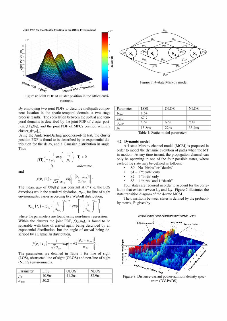
Figure 8: Distance-variant power-azimuth density spec-trum (DV-PADS)

watAaopcd 4Toptss(dTccomwTosodTogOnp
presence of a LOS path causes the channel sounder to miss paths with relatively low powers as the dynamic range of the channel sounder is finite (i.e. 40 dB). As diffuse reflections dominate in the OLOS and NLOS scenarios, the strongest paths detected by the channel sounder have approximately the same power. Therefore, paths with relatively low power can still be detected by the channel sounder provided they fall within the dynamic range. Under the LOS condition, M = 3 is sufficient, while for the OLOS and NLOS cases, at least M = 8 is required in order to ensure P converges. These values were verified by simula-tion results by increasing M until the value of P did not change significantly. For example, under the LOS condition it was observed that all elements of P estimated at M = 3 and M = 4 (i.e. P3 and P4, respectively) do not vary by more than 15%. Increasing M further does not alter the value of P sig-
Figure 9: Distance-variant power-delay density spectrum (DV-PDDS)
{ }
00 01 02 03
10 11 12 13
20 21 22 23
30 31 32 33
ij
p p p p
p p p pp p p p p
p p p p
= =
P (1) en
here i and j are state indices, and is the probability that process currently in state i will occupy state j after its next ransition.
ijp
nalysis of the measurement data shows that multiple births nd deaths can occur between two consecutive FDBs. In rder to account for this, a multiple step (M-step) MCM is roposed. By applying the 4-state MCM M times, both the orrelation between LB and LD as well as multiple births and eaths will be achieved.
.3 Model parameters he measurement data were fitted to (1) through solving a set f 29 over-determined nonlinear equations. The resulting arameter set describes the 4-state MCM parameters required o generate a set of multipath births and deaths that have imilar characteristics to the measured data itself. F hows the distance-variant power-azimuth density spectrum DV-PADS) and F , the distance-variant power-delay ensity spectrum (DV-PDDS) for a sample measurement file. he DV-PDDS shows that the TOA of the strongest LOS omponent increases as the trolley moves along its trajectory, orresponding to the trolley moving away from the RX. Also bservable in the graph are the higher order reflections. The ajor first order reflection is due to a reflection off the wall ith the entrance door. This accounts for the decrease in OA as the trolley moves further away from the RX. On the ther hand, the major second order reflection is due to the ignal being first reflected by the wall behind the RX (first rder), and then reflected again by the wall with the entrance oor (second order) before arriving at the RX.
igure 8
igure 9
nifica
NLOS
he figure also illustrates the appearance and disappearance f multipath components in the angular temporal plane. In eneral, larger values of LB and LD were obtained for the LOS and NLOS scenarios when compared to the LOS sce-ario. This is mainly due to a larger total number of multi-ath components in OLOS and NLOS environments. The
ntly. Thus, M = 3 is used as the upper limit of the step size to generate P for the LOS case. A similar observation was made for the OLOS and NLOS cases where the differ-
ce between P8 and P9 is insignificant. Therefore, M = 8 is used as the upper limit of the step size for the OLOS and
cases. An assessment of the performance of this approach can be
made by examining the total number of active paths for a
0 100 200 300 400 500 600 7000
5
10
15
20
25
30
35Dynamic Evolution of the Total Number of Active Paths − Office
Fast Doppler Block (FDB), n
To
tal N
um
ber
of
Act
ive
Pat
hs,
LT
0 100 200 300 400 500 600 7000
5
10
15
20
25
30
35Dynamic Evolution of the Total Number of Active Paths − Simulated
Fast Doppler Block (FDB), n
To
tal N
um
ber
of
Act
ive
Pat
hs,
LT
Figure 10: Total number of multipath components, meas-
ured and simulated

gtMrcrlt
F
igure 12 and Figure 13
4
DatntbcIupistFtpo
pWpitsUdbct
angle of arrival, and is well modelled by a truncated Gaus-sian distribution, shown as an inset in Figure 10. In order to model the power variation of a path within its lifespan, its power spectral density (PSD) is studied in order to determine an appropriate filter that is able to reproduce a set of random signals that exhibit the similar spectral charac-teristics. F illustrate the power varia-
−40 −30 −20 −10 0 10 200
5
10
15
20
25
30
35
40
45
50Spatio−Temporal Variation Within Path Lifespan − Office
Azimuth, φ [deg]
Rel
ativ
e D
elay
, τ [
ns]
Measurement DataBest Line Fit
−100 −50 0 50 1000
0.005
0.01
0.015
0.02
Spatio−temporal vector, ω
PD
F, f
(ω)
Estimated pdfData histogram
Figure 11: Variation of multipath component angle and time of arrival
iven scenario. F shows the number of paths de-ected in the measurement results, and a simulation using the
arkov parameter set extracted from this measurement envi-onment. Similar trends in the total number of multipaths an be observed in both measured results and in simulation esults, indicating a certain degree of confidence that the non-inear optimisation has produced results that are representa-ive of the practical environment.
igure 10
igure 11
igure 11
.4 Variation of multipath components within their life-span
uring the lifespan of a multipath component, its time of rrival, direction of arrival and power will vary due to mo-ion in the environment. This is a key element of the dy-amic nature of the channel, and will be different from the raditional Rayleigh fading based approaches, which are ased upon the concept of multiple coincident multipath omponents. n order to characterise the component variation, the meas-rement results were examined to find those multipath com-onents that had the longest lifetimes. These could be used n the analysis process as their longevity contributed to more tatistically significant data on how components vary over ime. irstly, the time and angle of arrival were examined to de-
ermine how these varied jointly for a given multipath com-onent: joint estimation is used as correlation between time f arrival and angle of arrival has already been established.
shows a scatter plot of all of the long lived multi-ath components’ parameters for an entire measurement run. ith the knowledge of the FDB number for each of these
oints, the variation of a single multipath component can be dentified. Drawn on this plot are the best fit lines indicating he direction of variation of multipath components in this patio-temporal plane. sing a definition of a spatio-temporal vector, ω, which escribes the angle between the angle of arrival axis and the est line fit in F , a description of how multipath omponents vary can be defined. It is found that the spatio-emporal vector is not dependent upon time of arrival or
tiitTsisivalaitdththmecth
0 0.2 0.4 0.6 0.8 1 1.2 1.4 1.6 1.8 20.3
0.4
0.5
0.6
0.7
0.8
0.9
1Power Variation of a Path Within Its Lifespan − Office
Relative distance travelled, x[m]N
orm
alis
ed p
ow
er, P
No
rm
Figure 12: Power variation of a single multipath compo-nent
on of a single path selected from the measurement data and s corresponding PSD (in logarithmic scale), respectively. hese figures show that only low frequency components are gnificant. Several other paths were also investigated and milar PSDs were observed. This implies that the power ariation of path within its lifespan can be well-modelled by simple LPF and a white noise source which exhibits a simi-r frequency response. The power variation of a path within s lifespan can be caused by several mechanisms. Firstly, ue to the motion of the MT along its trajectory that changes e reflection coefficients of some media. For example, as e trolley moves along the trajectory in the office environ-ent, reflections can be due to the walls, furniture, doors or
ven people in the surroundings. Thus, the building structure an cause a path to fade within its lifespan. Secondly, due to e finite spatio-temporal resolution of the measurement sys-
0 5 10 15 20 25−60
−50
−40
−30
−20
−10
0
Angular frequency, ψ, [cycle/meter]
No
rmal
ised
Po
wer
, PN
orm
[d
B]
Normalised Power Spectral Density − Office
Figure 13: Power spectral density of a single multipath component

REFERENCES tem, paths with closely spaced TOAs and AOAs are unable to be resolved. This causes multiple paths being detected as “a single path” which will fade due to changes in path lengths of the unresolvable components.
[1] R. B. Ertel, P. Cardieri, K. W. Sowerby, T. S. Rappaport and J. H. Reed, “Overview of spatial channel models for antenna array communication systems,” IEEE Pers. Com-mun., vol. 5, no. 1, pp. 10-22, Feb. 1998.
4.5 Model implementation [2] U. Martin, J. Fuhl, I. Gaspard, M. Haardt, A. Kuchar, C. Math, A. F. Molisch and R. Thomä, “Model scenarios for direction-selective adaptive antennas in cellular mobile communication systems – scanning the literature,” Wireless Pers. Commun., vol. 11, no. 1, pp. 109-129, Oct. 1999.
Parameters suitable for an office environment for the Markov model are; for line of sight,
=
2772.04165.03064.00000.08340.01663.00000.00000.04972.00000.05029.00000.00272.00367.00290.09039.0
LOSP [3] R. S. Thomä, D. Hampicke, A. Richter, G. Sommerkorn, A. Schneider, U. Trautwein and W. Wirnitzer, “Identification of time-variant directional mobile radio channels,” IEEE Trans. Instrum. Meas., vol. 49, no. 2, pp. 357-364, Apr. 2000. and for non-line of sight,
=
0411.09588.00000.00000.04715.05286.00000.00000.01131.00001.08869.00000.00018.00020.00029.09911.0
NLOSP
[4] C. M. Tan, M. A. Beach and A. R. Nix, “Indoor dynamic SIMO measurement and samples of post-processed results,” Internal report for Mobile VCE Core II WP3.1.1 Deliverable, Jan. 2002. [5] C. C. Chong, D. I. Laurenson, C. M. Tan, S. McLaugh-lin, M. A. Beach and A. R. Nix, “Joint detection-estimation of directional channel parameters using the 2-D frequency domain SAGE algorithm with serial interference cancella-tion,” in Proc. IEEE Intl. Conf. Commun. (ICC 2002), New York, USA, Apr. 2002, pp. 906-910.
Using these matrices, the M-step model can be run to pro-duce birth-death statistics of multipath components. Parame-ters for new components are selected from the joint distribu-tion functions defined for static environments, and their dy-namic evolution defined from the spatio-temporal angle and power spectral density defined above. The resulting set of multipath components can then be used as a directional channel implementation as input to a system simulation
[6] C.M. Tan, M.A. Beach, and A.R. Nix, “Multipath pa-rameters estimation with a reduced complexity unitary-SAGE algorithm,” European Transactions on Telecommuni-cations, Vol 14, pp. 515-528, January 2004. [7] S. Haykin, Adaptive Filter Theory, 4th ed., New York: Prentice Hall, 2001.
5. CONCLUSIONS
This paper has described a measurement and a modelling approach for producing detailed dynamic channel models that can be employed in antenna array based simulation sys-tems. The measurement system produces data in a form that allows for joint distributions between angle of arrival, angle of departure and time of flight to be formulated, the result-ing distributions being then used to create a channel model. MIMO measurements have indicated that there is strong correlation between angle of departure and angle of arrival of multipath components; this information should be incor-porated into future channel models in order to better test practical system implementations. A channel modelling approach has been described, with data fitting it to SIMO measurements, showing how correlated time of arrival and angle of arrival information can be used to generate realisa-tions of multipath channels.
[8] C. C. Chong, C. M. Tan, D. I. Laurenson, S. McLaugh-lin, M. A. Beach, A. R. Nix, “A New Statistical Wideband Spatio-Temporal Channel Model for 5GHz Band WLAN Systems”, IEEE J. Select. Areas Commun., vol. 21, no. 2, pp. 139-150, Feb. 2003.
6. ACKNOWLEDGEMENTS
The work reported in this paper has formed part of the Wire-less Access area of the Core 2 Research Programme of the Virtual Centre of Excellence in Mobile & Personal Commu-nications, Mobile VCE, www.mobilevce.com, whose fund-ing support, including that of EPSRC, is gratefully acknowl-edged. Fully detailed technical reports on this research are available to Industrial Members of Mobile VCE. Chia Chin Chong would also gratefully acknowledge funding from a Vodafone Scholarship.