Embed Size (px)
DESCRIPTION
Direct Volume Rendering Joe Michael Kniss [email protected] http://www.cs.utah.edu/~jmk Scientific Computing and Imaging Institute University of Utah. Outline. What is Volume Rendering? Shading models Current hardware methods Visualization 2001 presentation. What?. Volume Rendering. - PowerPoint PPT Presentation
Citation preview
Direct Volume Rendering
Joe Michael [email protected]
http://www.cs.utah.edu/~jmk
Scientific Computing and Imaging InstituteUniversity of Utah
Outline
1. What is Volume Rendering?
2. Shading models
3. Current hardware methods
4.Visualization 2001 presentation
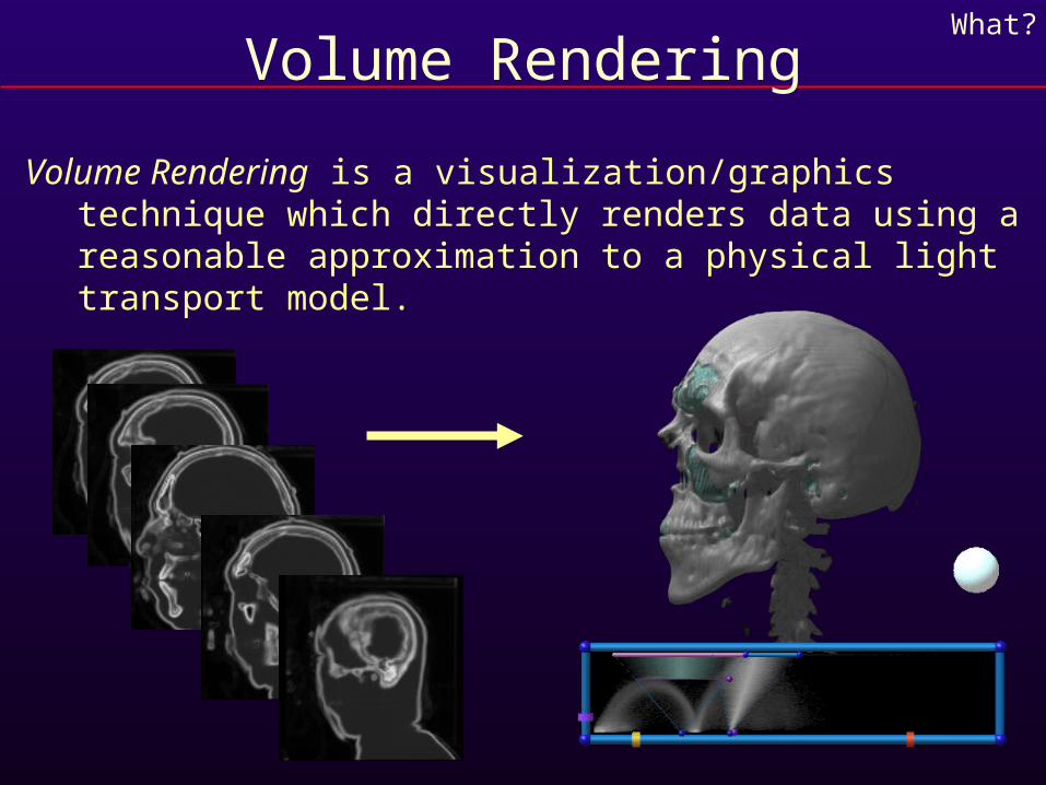
Volume Rendering
Volume Rendering is a visualization/graphics technique which directly renders data using a reasonable approximation to a physical light transport model.
What?
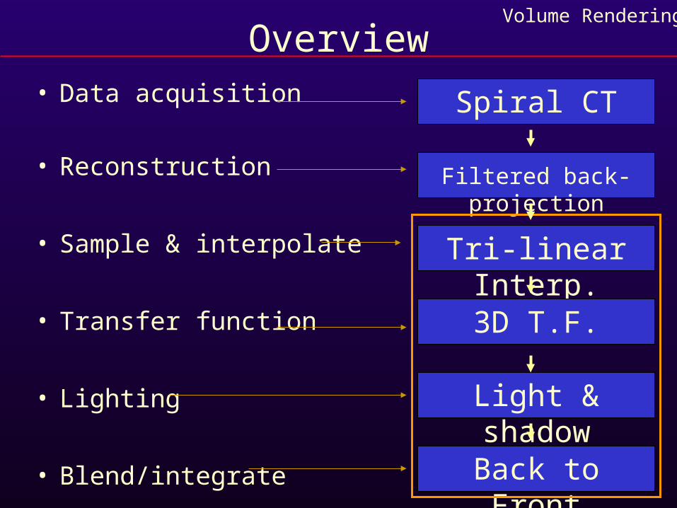
Overview• Data acquisition
• Reconstruction
• Sample & interpolate
• Transfer function
• Lighting
• Blend/integrate
Volume Rendering
Spiral CT
Filtered back-projection
Tri-linear Interp.
3D T.F.
Light & shadow
Back to Front
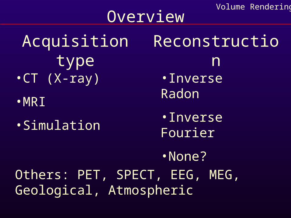
OverviewVolume Rendering
Acquisition type Reconstruction
•CT (X-ray)
•MRI
•Simulation
•Inverse Radon
•Inverse Fourier
•None?
Others: PET, SPECT, EEG, MEG, Geological, Atmospheric
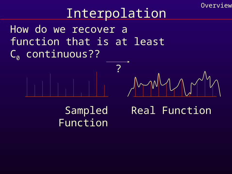
InterpolationOverview
Sampled Function
How do we recover a function that is at least C0 continuous??
Real Function
?
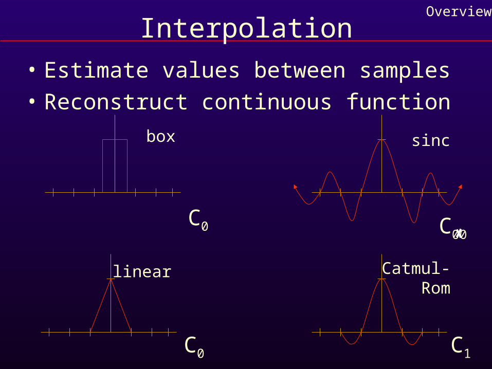
Interpolation
• Estimate values between samples
• Reconstruct continuous function
Overview
box
linear
sinc
Catmul-Rom
C0
C0 C1
C00
Interpolation
• Estimate values between samples
• Reconstruct continuous function
Overview
box
linear
sinc
Catmul-Rom
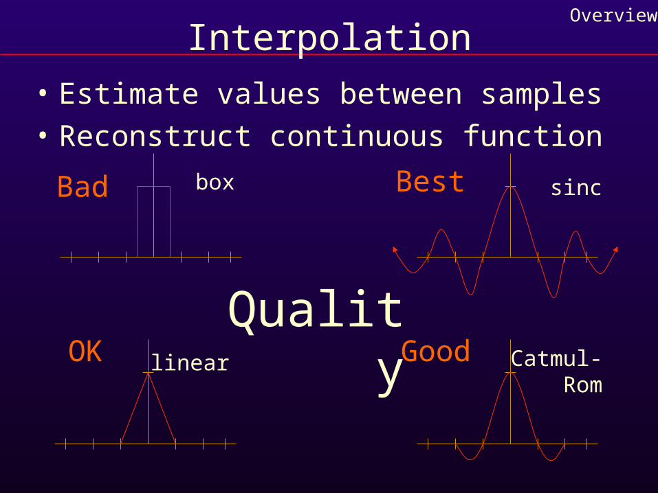
Bad
OK Good
Best
Quality
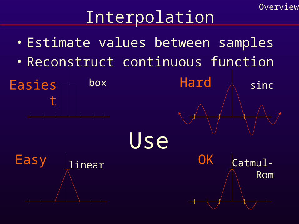
Interpolation
• Estimate values between samples
• Reconstruct continuous function
Overview
box
linear
sinc
Catmul-Rom
Easiest
Easy OK
Hard
Use

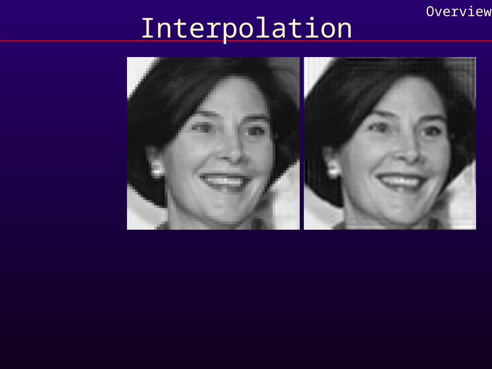
InterpolationOverview
Sampled Function
Laura Bush
InterpolationOverview
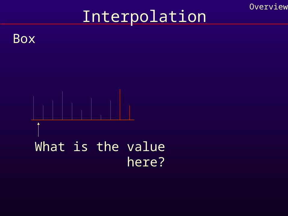
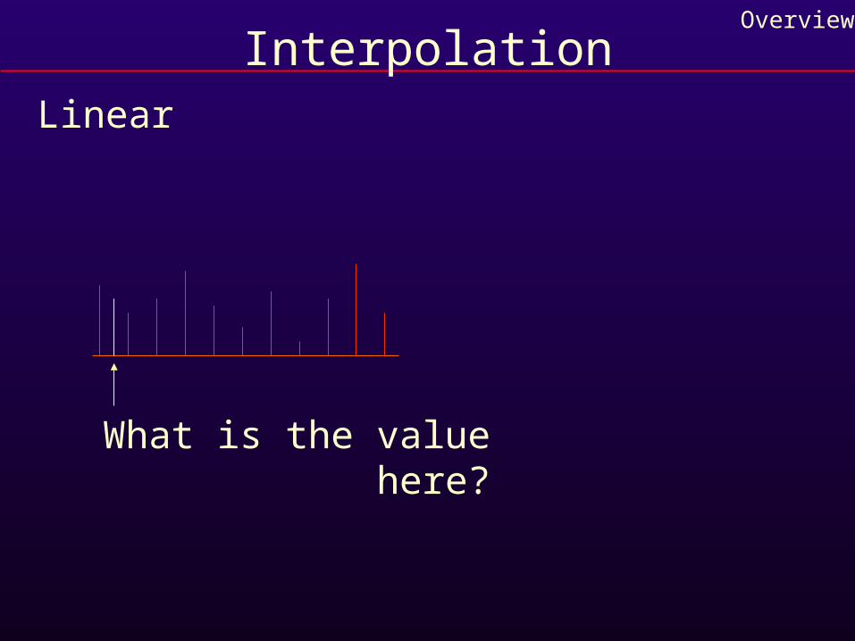
Box
What is the value here?
InterpolationOverview
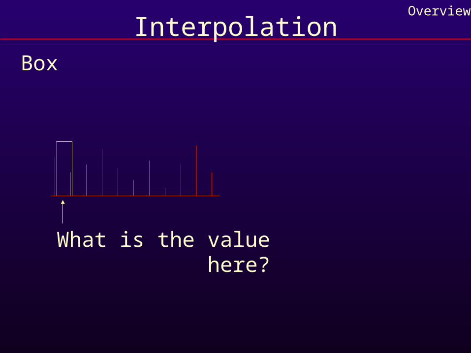
Box
What is the value here?
InterpolationOverview
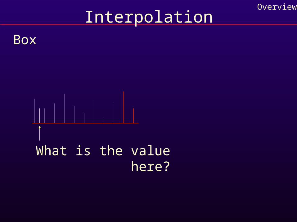
Box
What is the value here?
InterpolationOverview
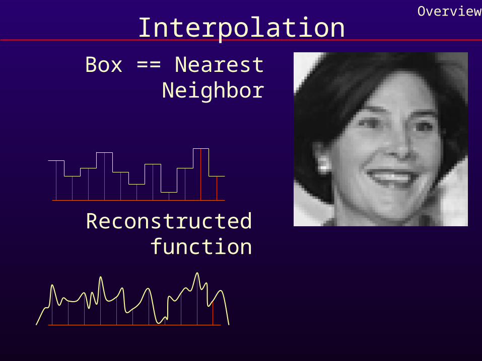
Box == Nearest Neighbor
Reconstructed function

InterpolationOverview
Linear
What is the value here?

InterpolationOverview
Linear
What is the value here?
InterpolationOverview
Linear
What is the value here?
InterpolationOverview
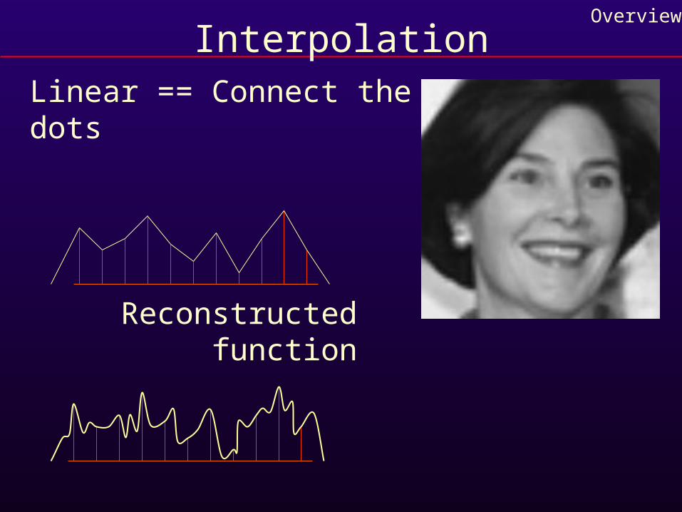
Linear == Connect the dots
Reconstructed function
InterpolationOverview
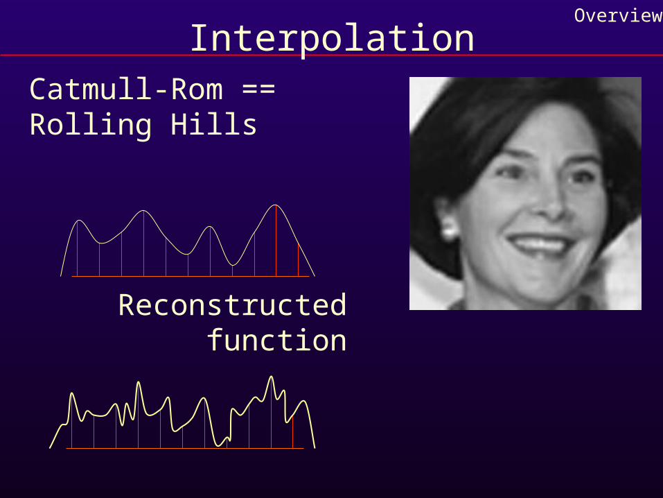
Catmull-Rom == Rolling Hills
Reconstructed function
InterpolationOverview
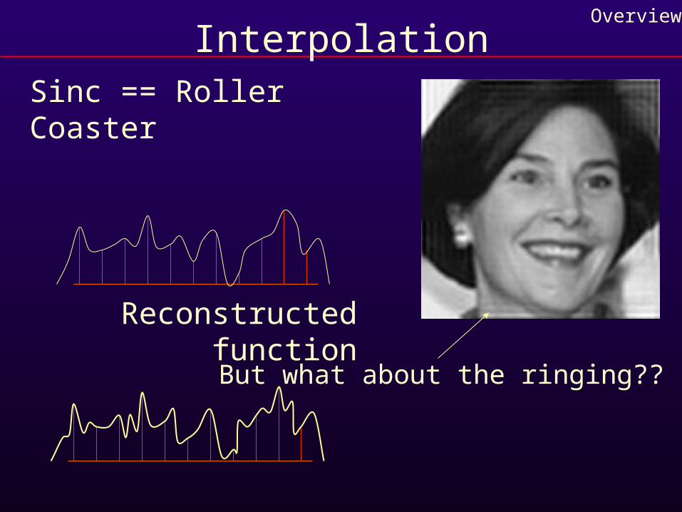
Sinc == Roller Coaster
Reconstructed function
But what about the ringing??
InterpolationOverview
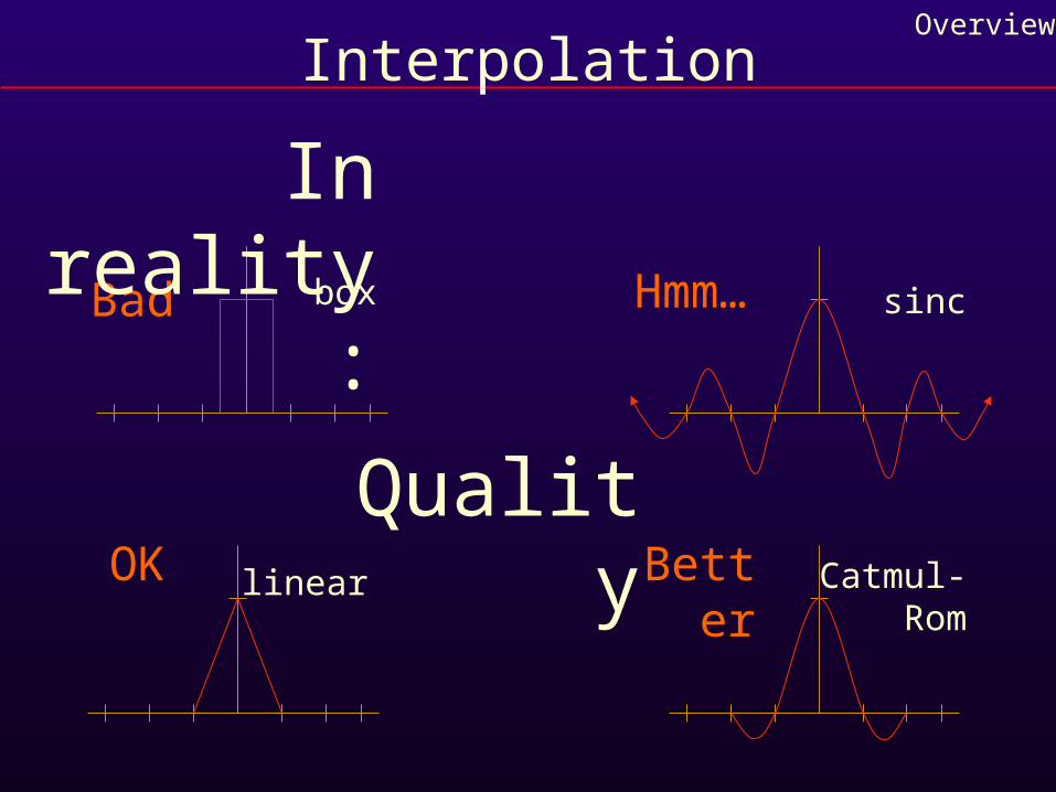
InterpolationOverview
box
linear
sinc
Catmul-Rom
Bad
OK Better
Hmm…
Quality
In reality:
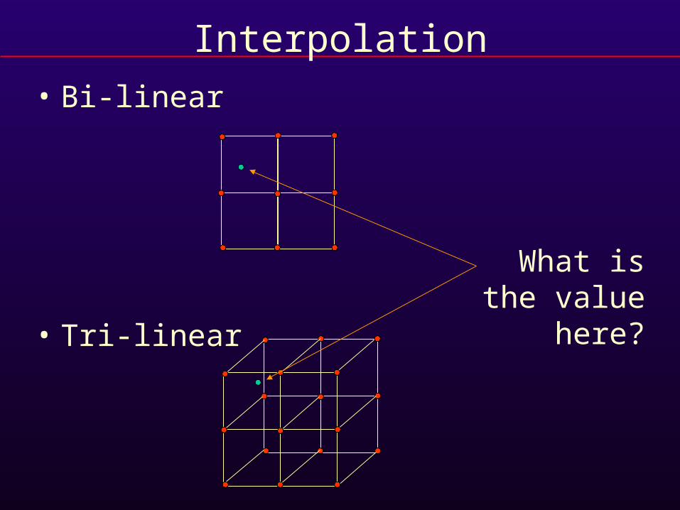
Interpolation
• Bi-linear
• Tri-linear
What is the value here?
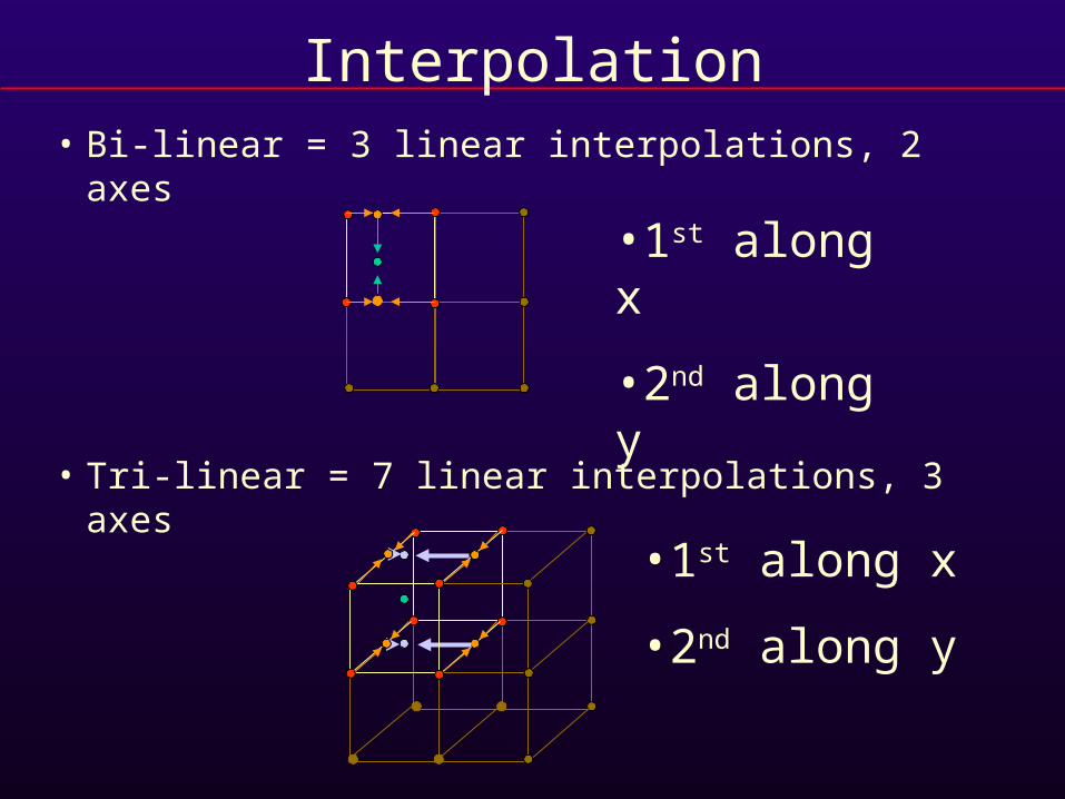
• Bi-linear = 3 linear interpolations, 2 axes
• Tri-linear = 7 linear interpolations, 3 axes
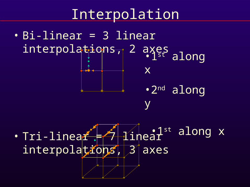
Interpolation
•1st along x
•2nd along y
•1st along x
• Bi-linear = 3 linear interpolations, 2 axes
• Tri-linear = 7 linear interpolations, 3 axes
Interpolation
•1st along x
•2nd along y
•1st along x
•2nd along y
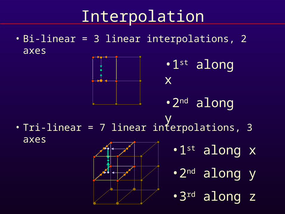
• Bi-linear = 3 linear interpolations, 2 axes
• Tri-linear = 7 linear interpolations, 3 axes
Interpolation
•1st along x
•2nd along y
•1st along x
•2nd along y
•3rd along z
Transfer Function
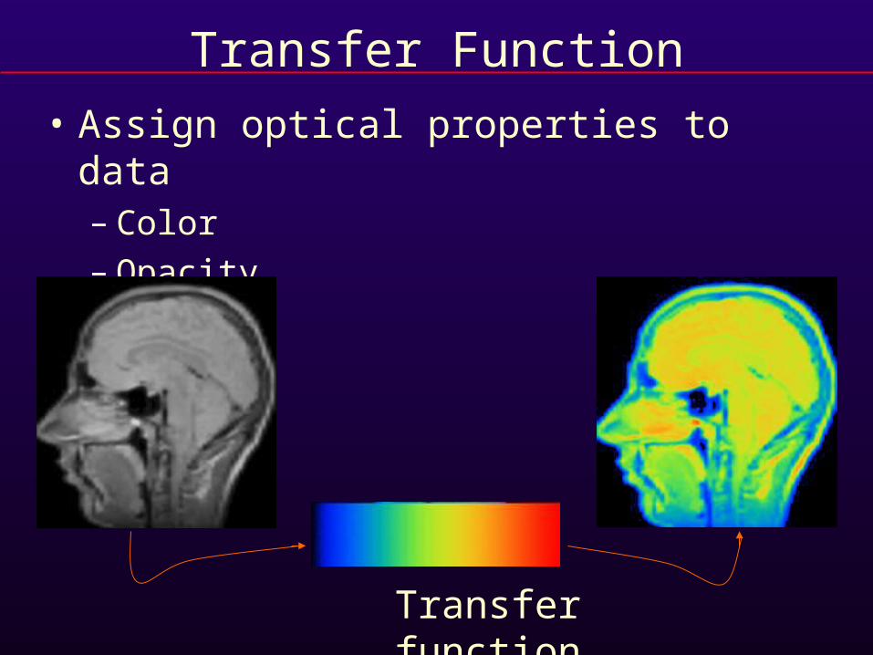
• Assign optical properties to data– Color– Opacity
Transfer function
Transfer Function
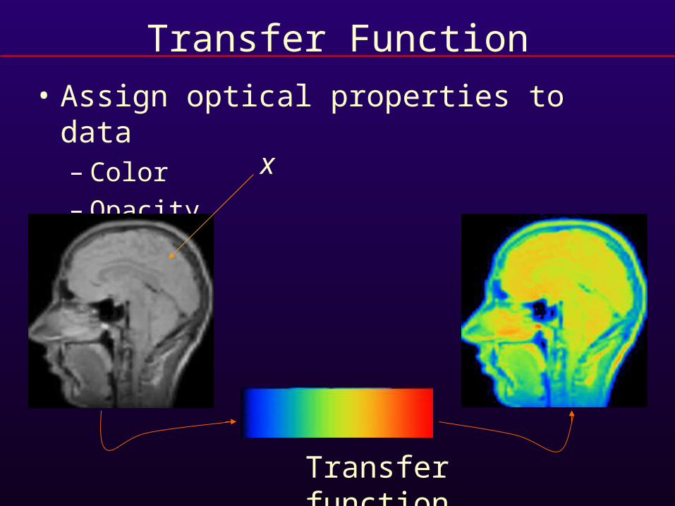
• Assign optical properties to data– Color– Opacity
Transfer function
x

Transfer Function
• Assign optical properties to data– Color– Opacity
Transfer function
T(x)
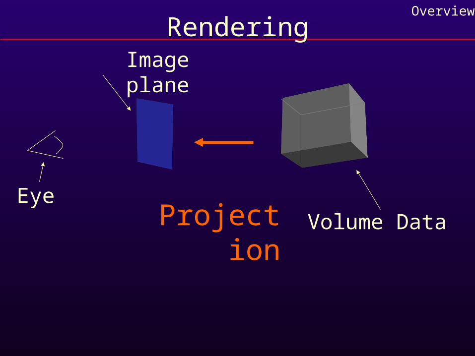
RenderingOverview
Volume DataEye
Image plane
Projection
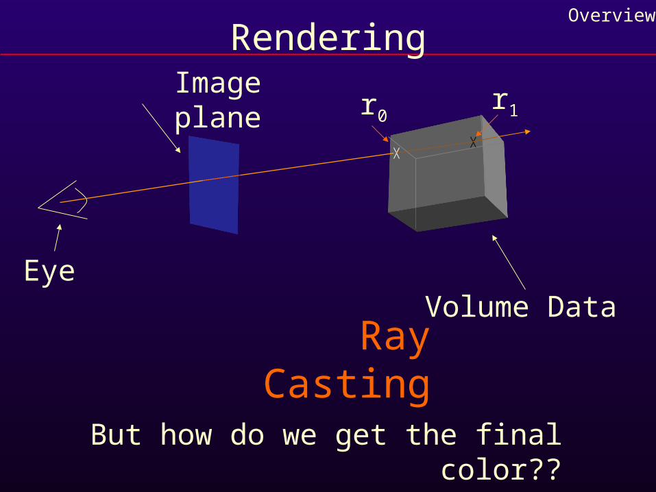
RenderingOverview
Volume DataEye
Image plane
Ray Casting
But how do we get the final color??
r0r1
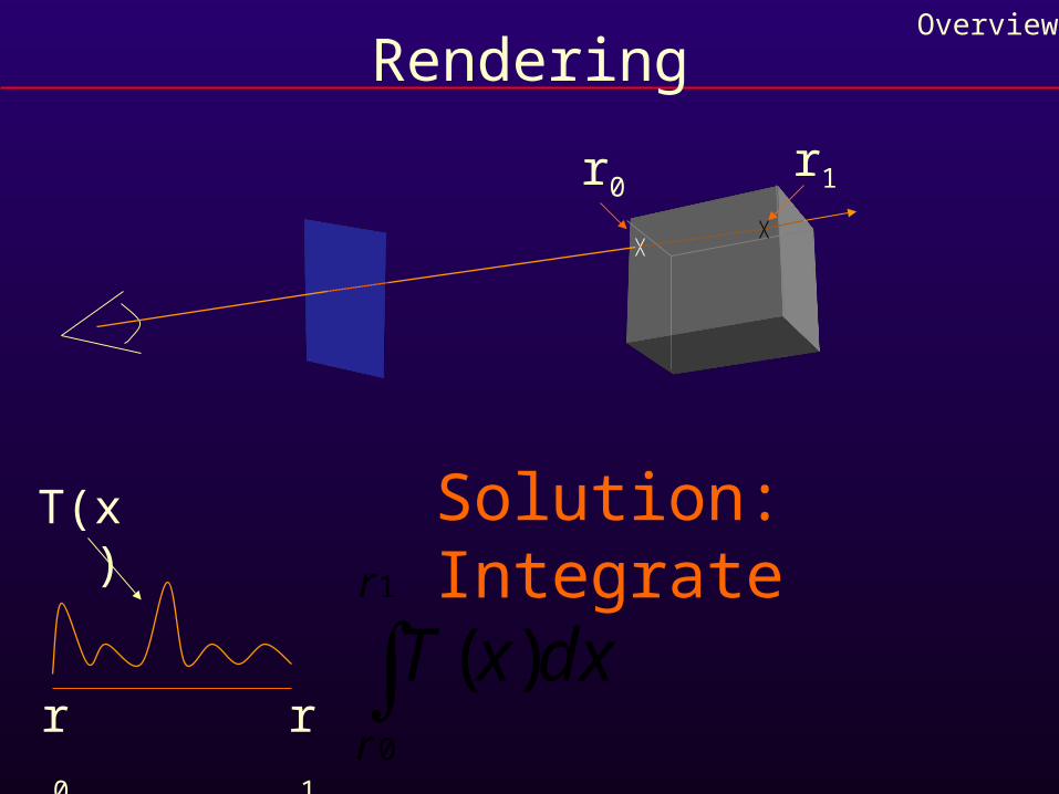
RenderingOverview
Solution: Integrate
r0 r11
0
)(r
r
dxxT
r0r1
T(x)
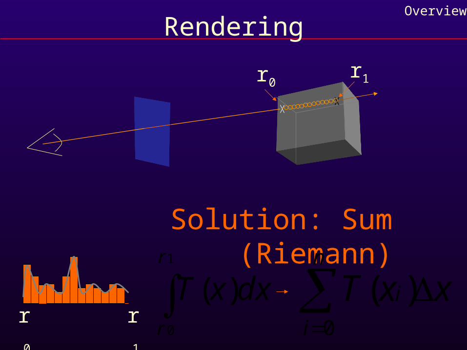
RenderingOverview
Solution: Sum (Riemann)
r0r1
r0 r11
0
)(r
r
dxxT xxTn
i
i 0
)(
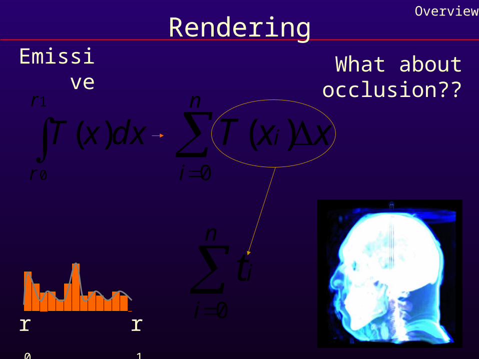
RenderingOverview
r0 r1
1
0
)(r
r
dxxT xxTn
i
i 0
)(
Emissive What about occlusion??
n
i
it0
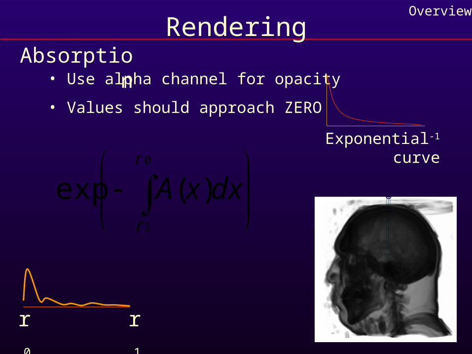
RenderingOverview
r0 r1
Absorption• Use alpha channel for opacity
• Values should approach ZERO
Exponential-1 curve
0
1
)(expr
r
dxxA
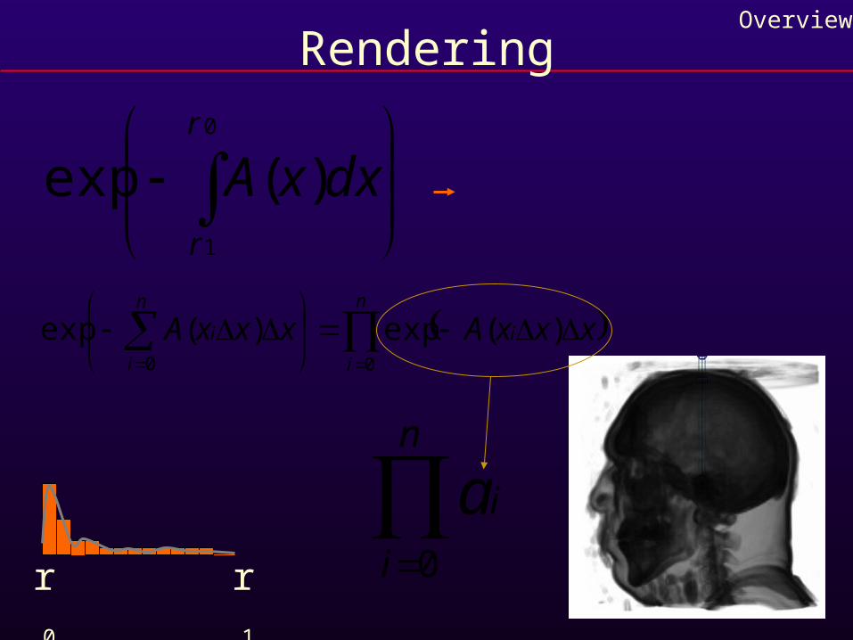
RenderingOverview
r0 r1
0
1
)(expr
r
dxxA
n
i
i
n
i
i xxxAxxxA00
)(exp)(exp
n
i
ia0
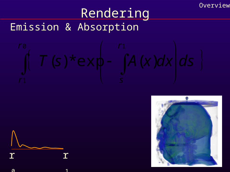
RenderingOverview
r0 r1
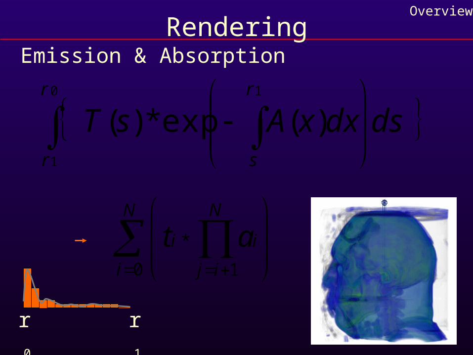
Emission & Absorption
dsdxxAsTr
s
r
r
10
1
)(exp*)(
RenderingOverview
Emission & Absorption
r0 r1
N
i
N
ij
ii at0 1
*
dsdxxAsTr
s
r
r
10
1
)(exp*)(
RenderingOverview
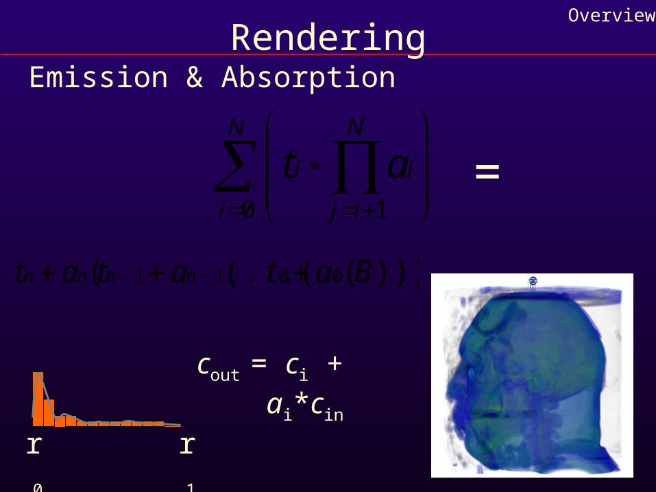
Emission & Absorption
r0 r1
))))((...(( 0011 Batatat nnnn
cout = ci + ai*cin
N
i
N
ij
ii at0 1
* =
RenderingOverview
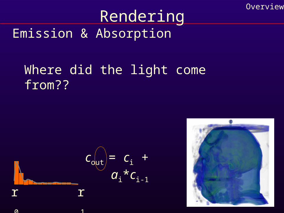
Emission & Absorption
r0 r1
cout = ci + ai*ci-1
Where did the light come from??
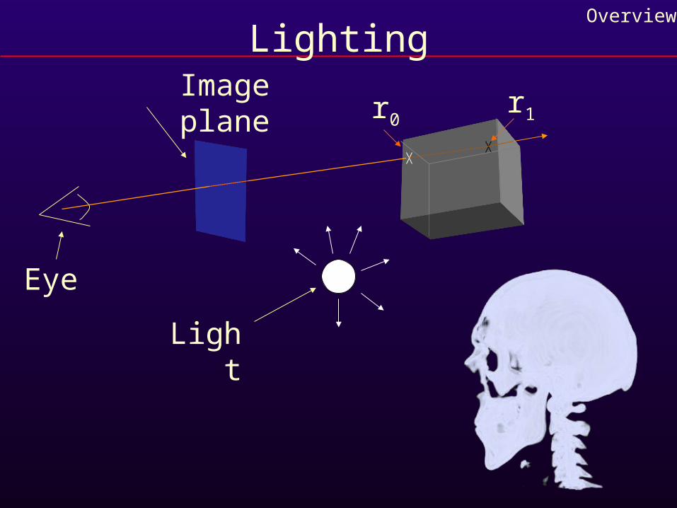
LightingOverview
Eye
Image planer0
r1
Light
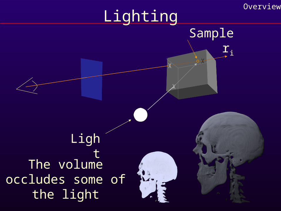
LightingOverview
Light
Sample ri
The volume occludes some of the light
N
i
N
ij
i
L
k
ki aat0 1
*
0
*
dsdxxAdttAsTr
s
r
r
l
s
00
1
0
)(exp*)(exp*)(
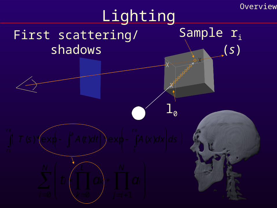
LightingOverview
Sample ri (s)First scattering/ shadows
l0
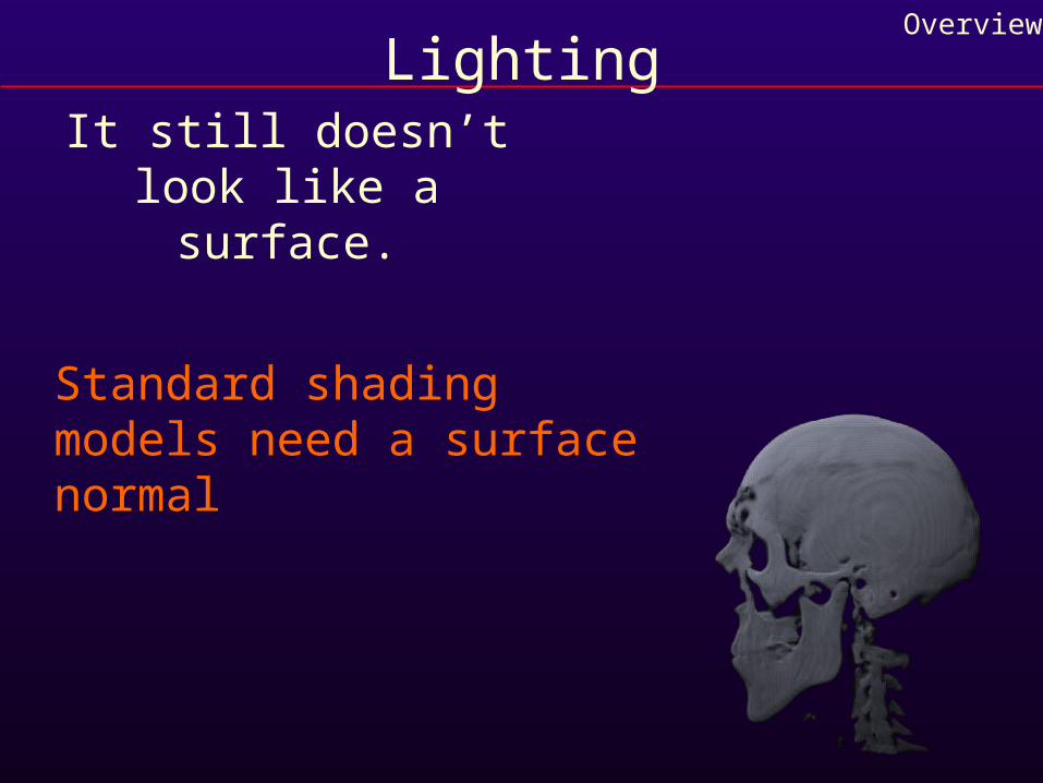
LightingOverview
It still doesn’t look like a surface.
Standard shading models need a surface normal
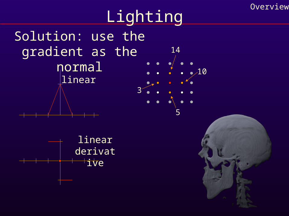
LightingOverview
Solution: use the gradient as the normal
linear
linear derivative
14
10
5
3
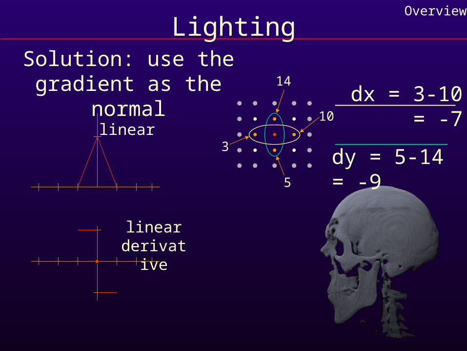
LightingOverview
Solution: use the gradient as the normal
linear
linear derivative
14
10
5
3
dx = 3-10 = -7
dy = 5-14 = -9
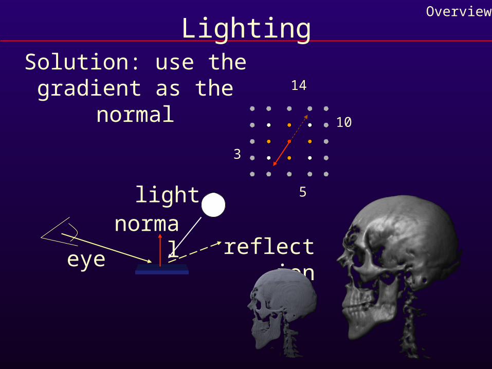
LightingOverview
Solution: use the gradient as the normal 14
10
5
3
normallight
eyereflection
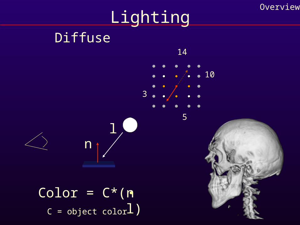
LightingOverview
Diffuse14
10
5
3
nl
Color = C*(n l)C = object color
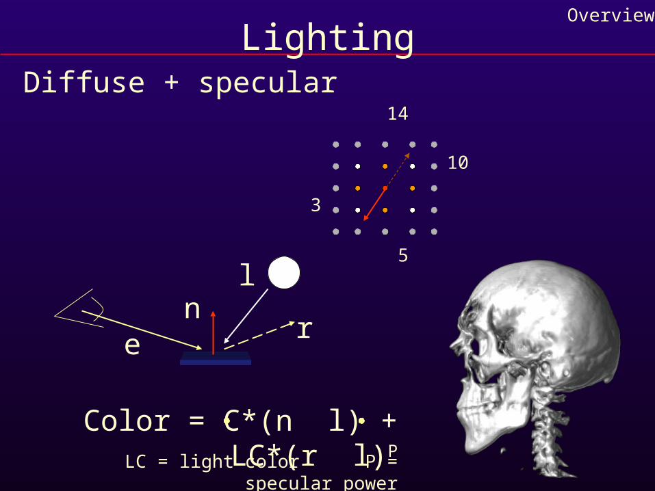
LightingOverview
Diffuse + specular14
10
5
3
nl
er
Color = C*(n l) + LC*(r l)P
LC = light color P = specular power
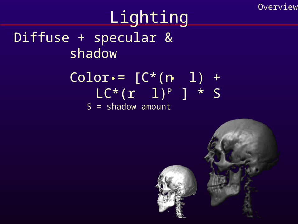
LightingOverview
Diffuse + specular & shadow
Color = [C*(n l) + LC*(r l)P ] * S
S = shadow amount
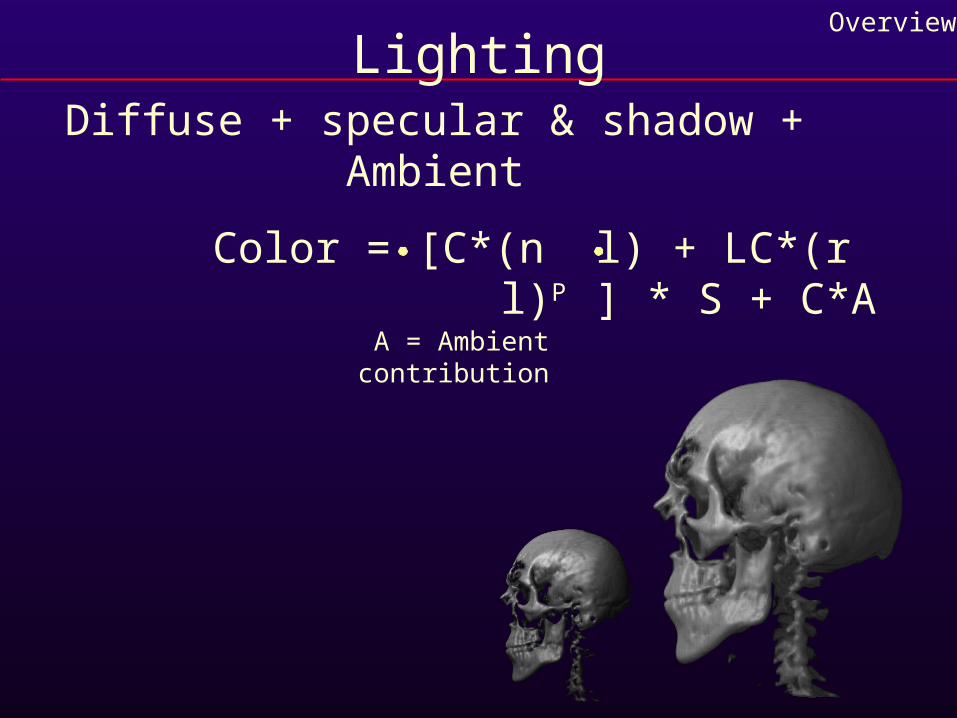
LightingOverview
Diffuse + specular & shadow + Ambient
Color = [C*(n l) + LC*(r l)P ] * S + C*A
A = Ambient contribution
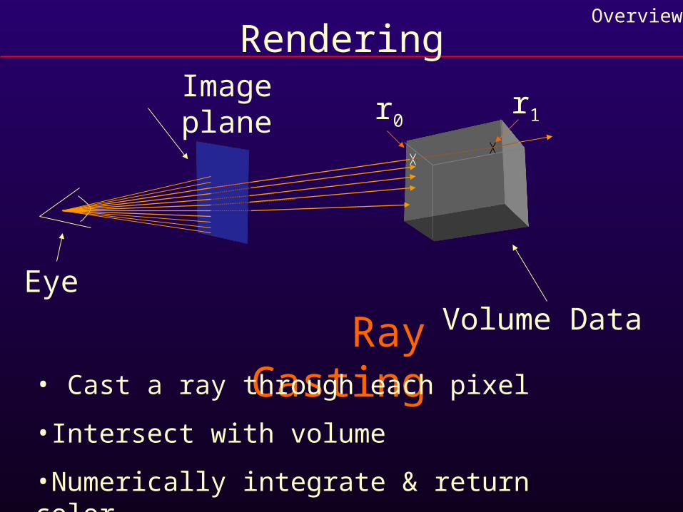
RenderingOverview
Volume DataEye
Image plane
Ray Casting
r0r1
• Cast a ray through each pixel
•Intersect with volume
•Numerically integrate & return color
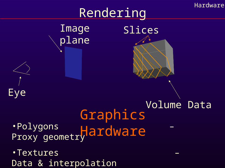
RenderingHardware
Volume DataEye
Image plane
Graphics Hardware•Polygons – Proxy geometry
•Textures – Data & interpolation
•Blending operations – Numerical integration
Slices
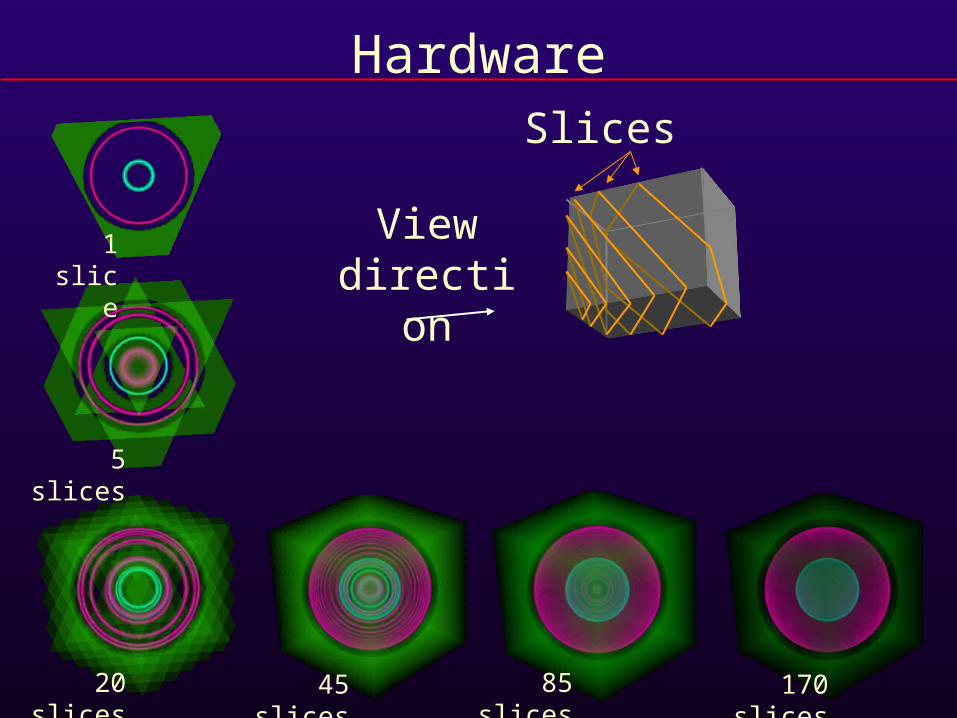
HardwareSlices
View direction
1 slice
5 slices
20 slices 45 slices 85 slices 170 slices
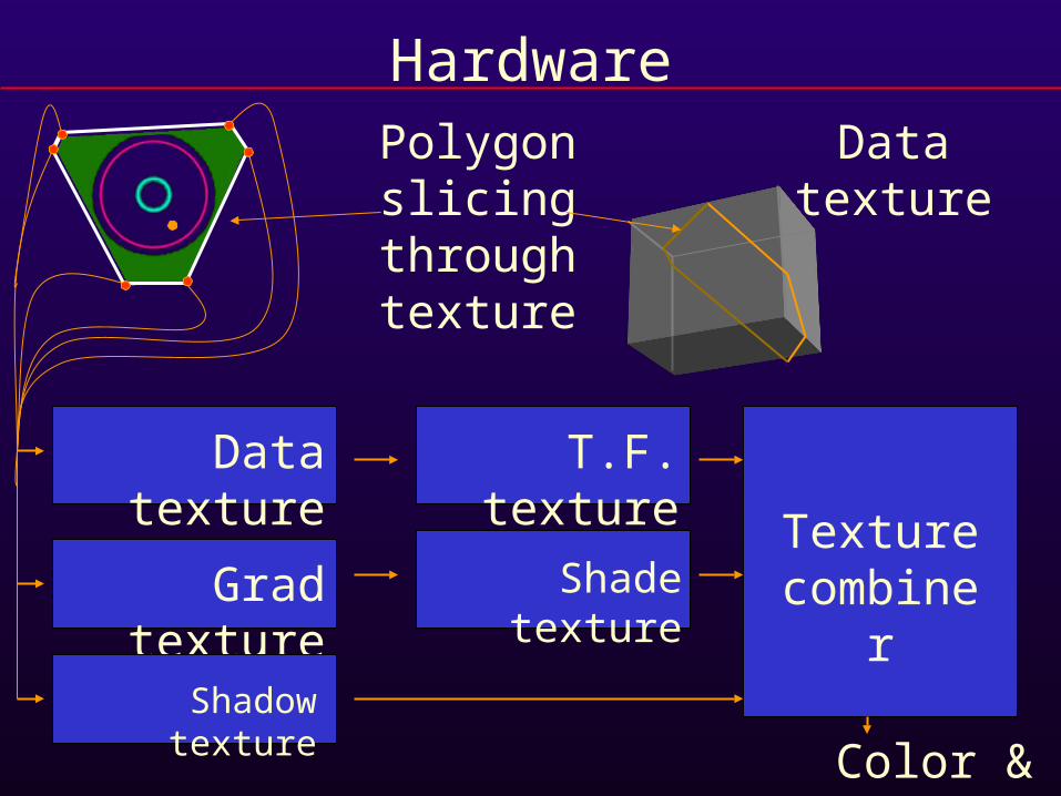
Hardware
Data texture
Grad texture
Shadow texture
T.F. texture
Shade textureTexture
combiner
Color & opacity
Data texture
Polygon slicing
through texture
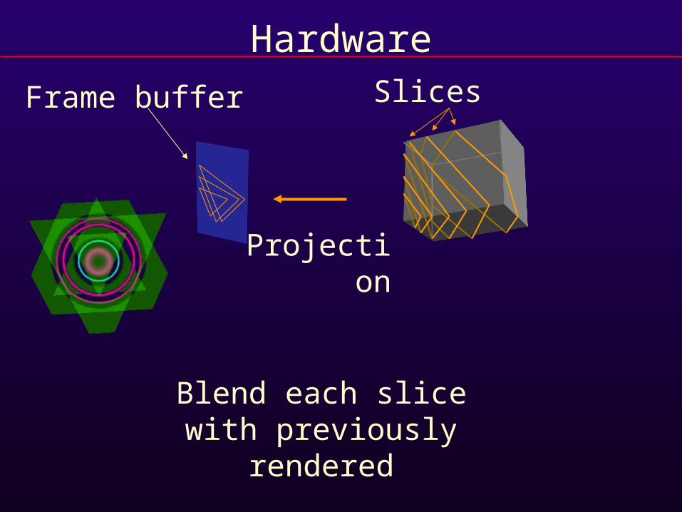
HardwareSlicesFrame buffer
Blend each slice with previously rendered
Projection
References
• Nelson Max, Optical Models for Direct Volume Rendering, IEEE Visualization and Computer Graphics (v1 #2 June 1995)
• Mark Levoy, Display of Surfaces from Volume Data, IEEE Computer Graphics and Applications (v8 #3 May 1988)
• Kenneth R. Castleman, Digital Image Processing, Prentice Hall (c1996 ISBN:0-13-211467-4)