Embed Size (px)
Citation preview
Master of Science Thesis KTH School of Industrial Engineering and Management
Energy Technology EGI-2014-103MSC EKV1064 Division of Heat & Power SE-100 44 STOCKHOLM
Effect of cooling charge air on the gas turbine performance and feasibility of using absorption refrigeration in the
“Kelanitissa” power station, Sri Lanka
Dinindu R. Kodituwakku
16.2
16.4
16.6
16.8
17
17.2
17.4
17.6
17.8
18
18.2
25 26 27 28 29 30 31 32
Act
ive
pow
er (M
W)
Ambient Temperature oC
Master of Science Thesis EGI-2014-103MSC EKV1064
Effect of cooling charge air on the gas turbine performance and feasibility of using
absorption refrigeration in the “Kelanitissa” power station, Sri Lanka
Dinindu R. Kodituwakku
Approved
2014-10-21
Examiner
Miroslav Petrov
Supervisors at KTH
Jens Fridh Commissioner
Open University of Sri Lanka
Local Supervisor
Dr. N S Senanayake
Abstract One of the drawbacks of the gas turbine is that performance drops rapidly when ambient air temperature increases. This is a major drawback for gas turbines operated in a tropical country like Sri Lanka. In Colombo, commercial capital of Sri Lanka where this study was carried out, the ambient temperature typically varies between 25 0C and 32 0C. The Kelanitissa gas turbine plant has single shaft gas turbines (GE MS5001 R) operated in open cycle which use diesel as fuel (designed for dual fuel) at a designed heat rate of 13,980 kJ/kWh and an electrical efficiency of 25.8%. The designed exhaust temperature is 513 0C. In this study, Kelanitissa gas turbine unit was used for assessment of the performance with the changes in ambient air temperature. Two approaches were used to study this phenomenon. Firstly, the performance parameters were calculated by using actual data acquired by the operation history of the power plant. Secondly, the performance was analyzed using thermodynamic principles. Then results of the two approaches were compared. The present performance values of the studied gas turbine, when compared to designed values, showed a very poor performance due to predominantly high ambient air temperatures. Originally designed for an efficiency of 25.8%, the maximum efficiency achieved at 33 0C was only 21.2%. This translates into a 4.6 %-point reduction in efficiency at 33 0C ambient temperature. Estimated cooling load for the proposed inlet air cooling is 679.87 RT. Cost per unit cooling load of the reference 2-stage direct-fired absorption system is $751-721 (according to 600RT-700RT). For the worst case scenario the value of $751 per RT and exhaust system constituting 98% of the cost of a market-ready direct fired system (Broad Inc., 2008) can be used. This results in $736/RT as the cost for an absorption chiller system driven by exhaust heat. Total cost for the 679.87 RT system is $ 500,370.72 (Rs. 65Mn). Payback period of the project is 11 years but the present value after 19 years is exceeding the project cost. Present value for 19 years is Rs. 65.86 Mn. Bringing down the temperature from an average of 270C to the ISO value of 15 0C would give Rs. 6 Mn of annual savings.

Acknowledgments
I would like to thank my supervisors first for the guidance in various ways to carry out
the work and for showing the correct sense where research should go. Then I would like to thank
Post Graduate Office, Royal Institute of Technology, Stockholm, Sweden for coordinating us
with the supervisors and course coordinators and various other supports.
Next I thank the Open University of Sri Lanka and ICBT campus for facilitating for the
course and linking with the local supervisors. Then I would thank engineers and employees at
Kelanitissa power station, Ceylon Electricity Board for helping me on collecting the operational
data of the turbines. And at last I would thank my friends and colleagues who supported me on
doing the research work.

2
Contents 1. INTRODUCTION ...................................................................................................................................... 4
1.1 GENERAL OVERVIEW ............................................................................................................................................................ 4 1.2 KELANITISSA GAS TURBINE POWER STATION .................................................................................................................. 5 1.3 PROBLEM STATEMENT ........................................................................................................................................................... 7 1.4 OBJECTIVES ............................................................................................................................................................................. 8
2. METHODOLOGY ..................................................................................................................................... 9
3. LITERATURE REVIEW .......................................................................................................................... 10
3.1 BACKGROUND AND PAST WORK ........................................................................................................................................ 10 3.2 CHARGE AIR COOLING METHODS ..................................................................................................................................... 13
Fogging system ............................................................................................................................................................................ 13 Evaporative cooler ...................................................................................................................................................................... 14 Mechanical refrigeration system (Direct type) ............................................................................................................................... 14 Mechanical refrigeration system (indirect type) ............................................................................................................................. 14 Mechanical refrigeration system with ice storage ........................................................................................................................... 15 Mechanical refrigeration system with chilled water storage ............................................................................................................ 15 LiBr absorption chiller ............................................................................................................................................................... 15
4. THERMODYNAMIC APPROACH ON THE GAS TURBINEAND INLET COOLING .................... 17
4.1 GAS TURBINE PERFORMANCE AND BRAYTON CYCLE ................................................................................................... 17 4.2 COOLING LOAD ESTIMATION FOR GAS TURBINE INLET COOLING.............................................................. 22 4.3 THERMODYNAMIC MODEL ANALYSIS FOR POWER OUTPUT AND EFFICIENCY ........................................................ 23
5. ANALYSIS OF DATA AND RESULTS ................................................................................................... 27
5.1 VARIATION OF ACTIVE POWER WITH AMBIENT TEMPERATURE .................................................................................. 27 5.2 HEAT RATE TEST .................................................................................................................................................................. 31 5.3 ACTUAL COOLING LOAD ESTIMATION ASSUMING INLET TEMPERATURE 270C ........................................................ 33 5.4 ECONOMIC ASPECTS OF THE PROJECT ............................................................................................................................. 35
Expected performance of the machines by inlet air cooling ............................................................................................................ 35 Economic feasibility analysis of the project ................................................................................................................................... 35 Project cost estimation ................................................................................................................................................................. 36
5.5 SYSTEM DESIGN ................................................................................................................................................................... 37 Exhaust flue gas conditions of the Kelanitissa GT ...................................................................................................................... 37 Selection of the Absorption refrigerating system ........................................................................................................................... 37 Components and layout of the system .......................................................................................................................................... 39
6. CONCLUDING REMARKS ...................................................................................................................... 41
6.1 POWER OUTPUT ................................................................................................................................................................... 41 6.2 EFFICIENCY ........................................................................................................................................................................... 42 6.3 FEASIBILITY ........................................................................................................................................................................... 43 6.4 FUTURE DEVELOPMENTS .................................................................................................................................................... 43
REFERENCES ............................................................................................................................................. 45
APPENDIX I ................................................................................................................................................ 47
EES EQUATIONS FOR POWER OUTPUT AND EFFICIENCY CALCULATION ..................................................................... 47
APPENDIX II ............................................................................................................................................... 50
EES EQUATIONS FOR COOLING LOAD CALCULATION ...................................................................................................... 50

3
Nomenclature 𝜼 - Efficiency 𝛄 - Specific heat ratio �̇�𝒔 - Sensible cooling load (kW) �̇�𝒂 - Volume flow rate of air at the ISO conditions (m3/kg) 𝒕𝒂𝒂,𝒅𝒃 - Dry bulb temperature of the ambient air (0C) 𝒕𝒄,𝒊 - Compressor inlet temperature (0C) 𝒗𝒂 - Specific volume of the wetted air per kilogram of dry air (m3/kg) Patm – Ambient pressure in (kPa) 𝑿𝒂𝒂,𝒅𝒃 - Specific humidity of the ambient air at its dry bulb temperature (kg/kg) 𝑴𝒗 - Molecular weight of the water vapor (kg/kmol) 𝑴𝒂 - Molecular weight of the air (kg/kmol) 𝑷𝒔 - The saturation vapor pressure at inlet air dry bulb temperature (kPa) 𝑪𝒑,𝒗 - Specific heat at constant pressure of the water vapor (kJ/kgK) 𝒙𝒄,𝒊𝒔 - Specific humidity at the compressor inlet temperature and (kg/kg) 𝑪𝒑,𝒘- Specific heat of liquid water at constant pressure (kJ/kgK) 𝒓𝒑 – Pressure ratio of the compressor Ta,in – Inlet air temperature (K) 𝑻𝒂𝒎𝒃 – Ambient temperature 𝑾𝒄𝒚𝒄 - Cyclic work 𝑾𝒕 - Turbine work 𝑾𝒄 - Compressor work 𝒉 – Enthalpy 𝑺 −Entropy 𝑻𝒇 – Firing temperature LHV – Lower heat value �̇�𝒇 – Fuel mass flow rate �̇�𝒂 – Air mass flow rate �̇�𝒈𝒂𝒔 – Gas mass flow rate (𝒓𝒑)𝒆𝒐𝒑𝒕 – Pressure ratio optimized to efficiency (𝒓𝒑)𝑷𝒘𝒐𝒑𝒕 – Pressure ratio optimized to power output 𝜼𝑡 – Turbine efficiency 𝜼𝑐 – Compressor efficiency 𝜼𝑐𝑦𝑐 – Cyclic efficiency PV – Present Value A – Annual return r – Discounted rate n – Number of years

4
1. Introduction
1.1 General Overview
A gas turbine (GT) is a heat engine that uses high-temperature, high-pressure gas as the
working fluid. Part of the heat supplied by the gas is converted to mechanical work. In most
cases, hot gas is produced by burning a fuel in air. This is why gas turbines are often referred to
as "combustion" turbines. Because gas turbines are compact, lightweight, quick-starting, and
simple to operate, they are widely used for power generation and in aircraft propulsion. The
capacity of gas turbines ranges from micro size to approximately 500 MW maximum per unit.
Gas turbine power plants are ideal for providing certain midrange and peaking electric
power to the grid for onsite power generation. Gas turbines are also responsive to load variations
and are very cost effective and feasible in combined cycle operation. They are commonly used in
combined cycle arrangements with steam Rankine bottoming cycle. There are some special cycles
like BIGCC (biomass integrated gasification combined cycle) where a gas turbines is utilized due
to its high power-to-weight ratio and high mass flow rate. Common fuels are NG (Natural gas),
Diesel (HSD) or sometimes HFO (heavy fuel oil) to power the gas turbines. The simple gas
turbine layout for power generation depicting main components is shown in Fig. 1 below.
Figure 1.1 Schematic layout of a simple gas turbine plant
5
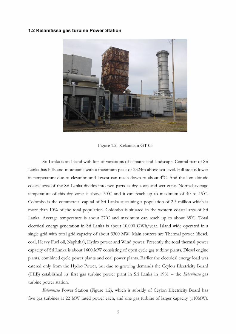
1.2 Kelanitissa gas turbine Power Station
Figure 1.2- Kelanitissa GT 05
Sri Lanka is an Island with lots of variations of climates and landscape. Central part of Sri
Lanka has hills and mountains with a maximum peak of 2524m above sea level. Hill side is lower
in temperature due to elevation and lowest can reach down to about 40C. And the low altitude
coastal area of the Sri Lanka divides into two parts as dry zoon and wet zone. Normal average
temperature of this dry zone is above 300C and it can reach up to maximum of 40 to 450C.
Colombo is the commercial capital of Sri Lanka sustaining a population of 2.3 million which is
more than 10% of the total population. Colombo is situated in the western coastal area of Sri
Lanka. Average temperature is about 270C and maximum can reach up to about 350C. Total
electrical energy generation in Sri Lanka is about 10,000 GWh/year. Island wide operated in a
single grid with total grid capacity of about 3300 MW. Main sources are Thermal power (diesel,
coal, Heavy Fuel oil, Naphtha), Hydro power and Wind power. Presently the total thermal power
capacity of Sri Lanka is about 1600 MW consisting of open cycle gas turbine plants, Diesel engine
plants, combined cycle power plants and coal power plants. Earlier the electrical energy load was
catered only from the Hydro Power, but due to growing demands the Ceylon Electricity Board
(CEB) established its first gas turbine power plant in Sri Lanka in 1981 – the Kelanitissa gas
turbine power station.
Kelanitissa Power Station (Figure 1.2), which is subsidy of Ceylon Electricity Board has
five gas turbines at 22 MW rated power each, and one gas turbine of larger capacity (110MW).
6
Those are grid connected and mostly started in peak hours to cater for the peak demand. Sri
Lanka as a third world country, electricity from open cycle gas turbine (Diesel) is an extravagance
solution for the energy demand. The CEB has to bare cost of about Rs.60/kWh ($0.50/kWh) per
unit. But the unit selling price for electricity is far below the production cost. Hence it is not
economical to run open cycle gas turbines and also environmental hazards due to high waste heat
rejection are involved. Hence these gas turbines should be modified in such a way so that to
increase their economic viability in operation and also to improve their environmental aspects.
Nowadays, waste heat from gas turbines can be used constructively in several ways. For example
in Combined Heat and Power plants, combined cycle power plants, chiller plants etc. All these
methods can optimize the use of energy from the fuel. But if we can increase the efficiency of the
existing gas turbine, it can directly deliver a cut down of energy cost. Charge air cooling is a
plausible method to increase the power output and the efficiency of the existing gas turbines.
Following specifications are from the 5 identical gas turbines mentioned above:
Model : GE MS5001 (Frame 5)
Make : John Brown
Rated output of Turbine : 22,480 kW
Generator Output : 25 MVA
Fuel : Auto Diesel
Year of Manufacture : 1980
This is a single shaft gas turbine operated in open cycle which is using diesel as fuel (designed for
dual fuel). It features an axial compressor with 16 stages and a turbine with 2 stages rotating at a
speed of 5100 rpm. Firing temperature is about 2,5000F (13710C) to 32000F (17600C) and turbine
inlet temperature is in the range 16500F - 17500F (8990C - 9540C). Designed heat rate of the gas
turbine is 13,980kJ/kWh at an efficiency of 25.8%. The designed exhaust temperature is 5130C.
For the study of GT performance with varying inlet temperature, one of these gas turbines
was chosen as reference. The gas turbine has been designed around a limiting firing temperature
(Tf), which ensures that the hot gas path parts are not subjected to excessive thermal stress, and
as a measure of Tf, the exhaust temperature Tx is used in the control system. It would not be
practical to directly measure Tf since this could be around 3000 oF (16490C) but by using 12
thermocouples around the exhaust plenum we can obtain an accurate indication of Tf through
Tx. As the unit is loaded up on a hot day it will reach the limiting firing temperature level at a
high exhaust temperature and it operates on a low load with low fuel consumption. On a cold day
the same limiting temperature will be reached at a lower Tx and it operates at maximum load with
high fuel consumption. So increasing the ambient temperature, the power output proportionately
7
reduces while increasing the heat rate and the exhaust gas temperature. In this case the gas
turbine lowers its output with the inlet temperature by two ways. One is due to lowering of the
air mass flow rate and the other is lowering of the power by lowering the fuel in order to keep
down the Tf within its safe limit.
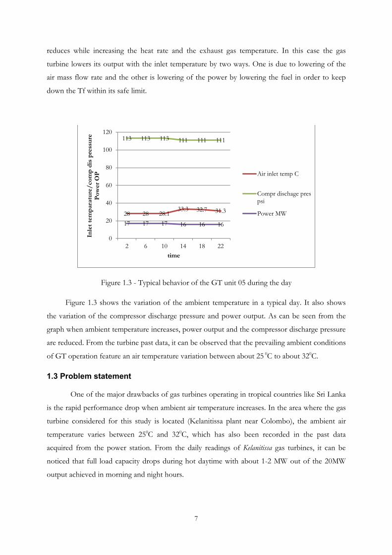
Figure 1.3 - Typical behavior of the GT unit 05 during the day
Figure 1.3 shows the variation of the ambient temperature in a typical day. It also shows
the variation of the compressor discharge pressure and power output. As can be seen from the
graph when ambient temperature increases, power output and the compressor discharge pressure
are reduced. From the turbine past data, it can be observed that the prevailing ambient conditions
of GT operation feature an air temperature variation between about 25 0C to about 320C.
1.3 Problem statement
One of the major drawbacks of gas turbines operating in tropical countries like Sri Lanka
is the rapid performance drop when ambient air temperature increases. In the area where the gas
turbine considered for this study is located (Kelanitissa plant near Colombo), the ambient air
temperature varies between 250C and 320C, which has also been recorded in the past data
acquired from the power station. From the daily readings of Kelanitissa gas turbines, it can be
noticed that full load capacity drops during hot daytime with about 1-2 MW out of the 20MW
output achieved in morning and night hours.
28 28 28.1 33.3 32.7 31.3
113 113 113 111 111 111
17 17 17 16 16 16
0
20
40
60
80
100
120
2 6 10 14 18 22
Inle
t tem
para
ture
/com
p di
s pr
essu
re
Pow
er O
P
time
Air inlet temp C
Compr dischage prespsi
Power MW

8
1.4 Objectives
This research and evaluation study will focus on the possible performance enhancement of
the reference gas turbine by supplying charge air cooling. Main objective is to derive the behavior
of the gas turbine with the ambient temperature variation. A thermodynamic model for the inlet
air cooling performance will then be developed and approximated by simulations. Further, the
use of available exhaust gas heat to drive the charge air cooler and its technical and economic
feasibility will be studied for analyzing the adoption of a practical absorption refrigeration system
in the Kelanitissa Power station.

9
2. Methodology
In this research the main focus was to investigate the present situation of the gas turbine inlet
cooling. As the first step, literature survey was carried out to study about the inlet cooling
methods, advantages and disadvantages in specific methods, theoretical background of the inlet
cooling, gas turbine operation. Relationship between inlet cooling and gas turbine performance
was analyzed and discussed.
One of the Kelanitissa gas turbine units was used for assessing the performance with the changes
in ambient air temperature. Two approaches were applied to study this phenomenon. Firstly,
changes were calculated by actual data acquired by the operation history of the power plant. The
required data needed for the analysis was acquired from the data sheets of the power plant and
from the machine manuals. These data were analyzed in view of determining the patterns of
variations of performance with air temperature. Secondly, the performance was analyzed using
thermodynamic principles. Then the results of the two approaches were compared.
In the next phase, energy calculations were performed to obtain the required level of the charge
air cooling and to select a suitable capacity of absorption chiller. Then the costs involved were
calculated. Finally, the technical and economic feasibility of the system were analyzed and
discussed in details.
10
3. Literature Review
3.1 Background and past work
Industrial gas turbines are usually rated according to ISO conditions, which are
(OMIDVAR, Bob, 2001):
1. Ambient dry bulb temperature: 150C
2. Relative humidity: 60%
3. Wet bulb temperature: 7.20C
4. Atmospheric pressure: 1.01325 bar (sea level)
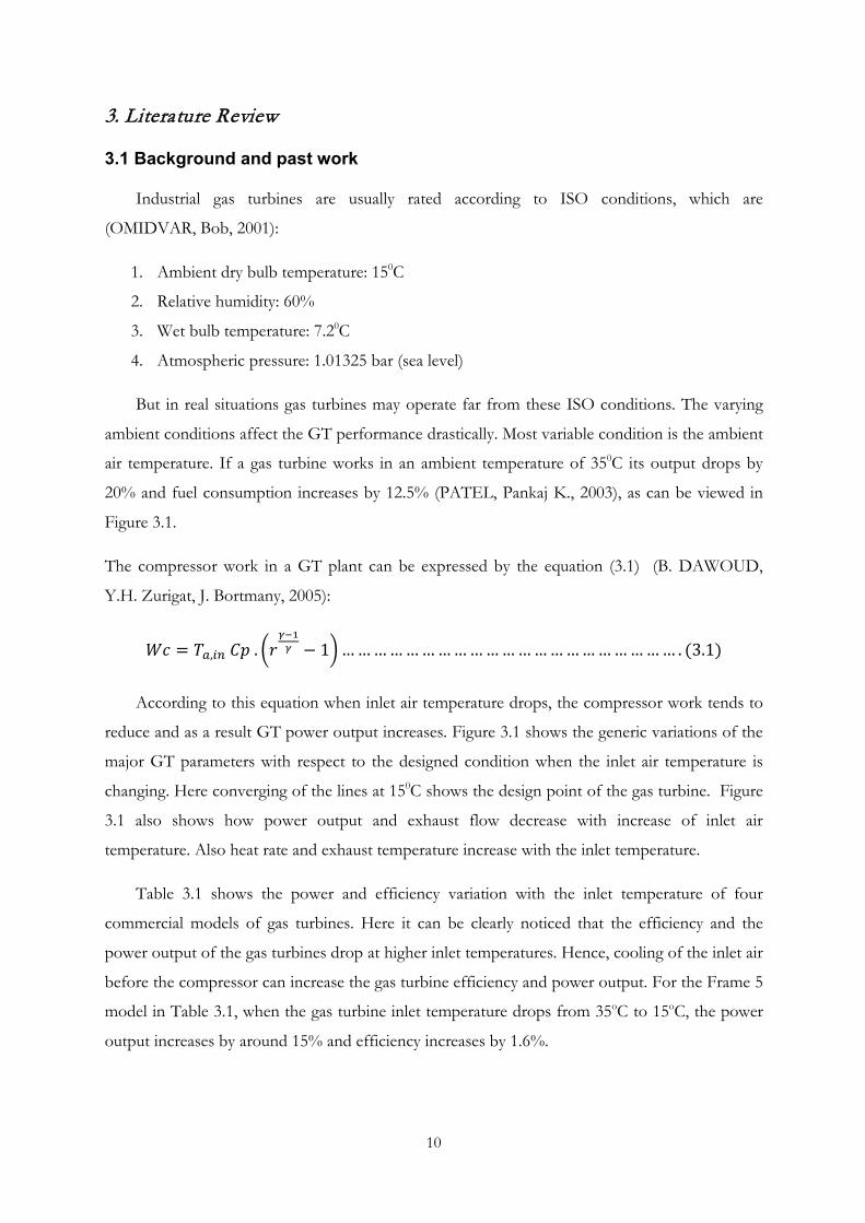
But in real situations gas turbines may operate far from these ISO conditions. The varying
ambient conditions affect the GT performance drastically. Most variable condition is the ambient
air temperature. If a gas turbine works in an ambient temperature of 350C its output drops by
20% and fuel consumption increases by 12.5% (PATEL, Pankaj K., 2003), as can be viewed in
Figure 3.1.
The compressor work in a GT plant can be expressed by the equation (3.1) (B. DAWOUD,
Y.H. Zurigat, J. Bortmany, 2005):
𝑊𝑐 = 𝑇𝑎,𝑖𝑛 𝐶𝑝 . �𝑟𝛾−1𝛾 − 1�… … … … … … … … … … … … … … … … … … … … … . (3.1)
According to this equation when inlet air temperature drops, the compressor work tends to
reduce and as a result GT power output increases. Figure 3.1 shows the generic variations of the
major GT parameters with respect to the designed condition when the inlet air temperature is
changing. Here converging of the lines at 150C shows the design point of the gas turbine. Figure
3.1 also shows how power output and exhaust flow decrease with increase of inlet air
temperature. Also heat rate and exhaust temperature increase with the inlet temperature.
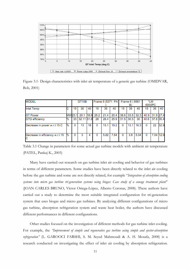
Table 3.1 shows the power and efficiency variation with the inlet temperature of four
commercial models of gas turbines. Here it can be clearly noticed that the efficiency and the
power output of the gas turbines drop at higher inlet temperatures. Hence, cooling of the inlet air
before the compressor can increase the gas turbine efficiency and power output. For the Frame 5
model in Table 3.1, when the gas turbine inlet temperature drops from 35oC to 15oC, the power
output increases by around 15% and efficiency increases by 1.6%.
11
Figure 3.1- Design characteristics with inlet air temperature of a generic gas turbine (OMIDVAR,
Bob, 2001)
Table 3.1 Change in parameters for some actual gas turbine models with ambient air temperature
(PATEL, Pankaj K., 2003)
Many have carried out research on gas turbine inlet air cooling and behavior of gas turbines
in terms of different parameters. Some studies have been directly related to the inlet air cooling
before the gas turbine and some are not directly related, for example “Integration of absorption cooling
systems into micro gas turbine tri-generation systems using biogas: Case study of a sewage treatment plant”
(JOAN CARLES BRUNO, Víctor Ortega-López, Alberto Coronas, 2008). These authors have
carried out a study to determine the most suitable integrated configuration for tri-generation
system that uses biogas and micro gas turbines. By analyzing different configurations of micro
gas turbine, absorption refrigeration system and waste heat boiler, the authors have discussed
different performances in different configurations.
Other studies focused on the investigation of different methods for gas turbine inlet cooling.
For example, the “Improvement of simple and regenerative gas turbine using simple and ejector-absorption
refrigeration” (L. GAROOCI FARSHI, S. M. Seyed Mahmoudi & A. H. Mosafa, 2008) is a
research conducted on investigating the effect of inlet air cooling by absorption refrigeration.
12
According to this study, gas turbine power output and efficiency were found to increase by 6-
10% and 1-5% respectively for a decrease of 10oC of inlet air temperature.
Al-Tobi, I. (2009) reported that gas turbine performance changes with inlet cooling
according to a study performed with simulation software called “Turbomatch” which is another
approach for analyzing this type of machines.
However, Thamir et al. (2011) reported that the efficiency was decreasing slightly with the
inlet cooling, but power output was increasing. It states “gas turbine intake air cooling may
cause a small decrease in efficiency because a lot of fuel is needed to bring compressor
exhaust gas equal to the same gas turbine entry temperature”. This statement is based on basic
energy calculation done on simple cycle gas turbine cycle based on shear theoretical basis.
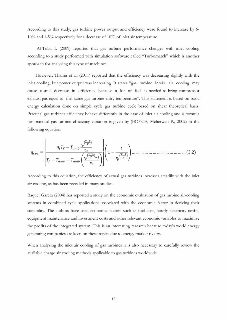
Practical gas turbines efficiency behave differently in the case of inlet air cooling and a formula
for practical gas turbine efficiency variation is given by (BOYCE, Meherwan P., 2002) in the
following equation:
η𝑐𝑦𝑐 =
⎣⎢⎢⎢⎢⎡
𝜂𝑡𝑇𝑓 − 𝑇𝑎𝑚𝑏𝑟𝑝
�𝛾−1𝛾 �
𝜂𝑐
𝑇𝑓 − 𝑇𝑎𝑚𝑏 − 𝑇𝑎𝑚𝑏 �𝑟𝑝
�𝛾−1𝛾 �−1
𝜂𝑐�⎦⎥⎥⎥⎥⎤
�1 −1
𝑟𝑝�𝛾−1𝛾 �
�… … … … … … … … … … … … … (3.2)
According to this equation, the efficiency of actual gas turbines increases steadily with the inlet
air cooling, as has been revealed in many studies.
Raquel Gareta (2004) has reported a study on the economic evaluation of gas turbine air-cooling
systems in combined cycle applications associated with the economic factor in deriving their
suitability. The authors have used economic factors such as fuel cost, hourly electricity tariffs,
equipment maintenance and investment costs and other relevant economic variables to maximize
the profits of the integrated system. This is an interesting research because today’s world energy
generating companies are keen on these topics due to energy market rivalry.
When analyzing the inlet air cooling of gas turbines it is also necessary to carefully review the
available charge air cooling methods applicable to gas turbines worldwide.
13
3.2 Charge air cooling methods
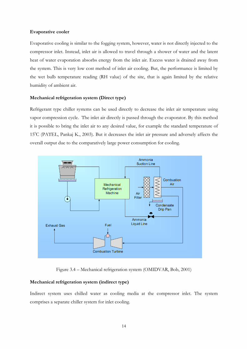
Fogging system
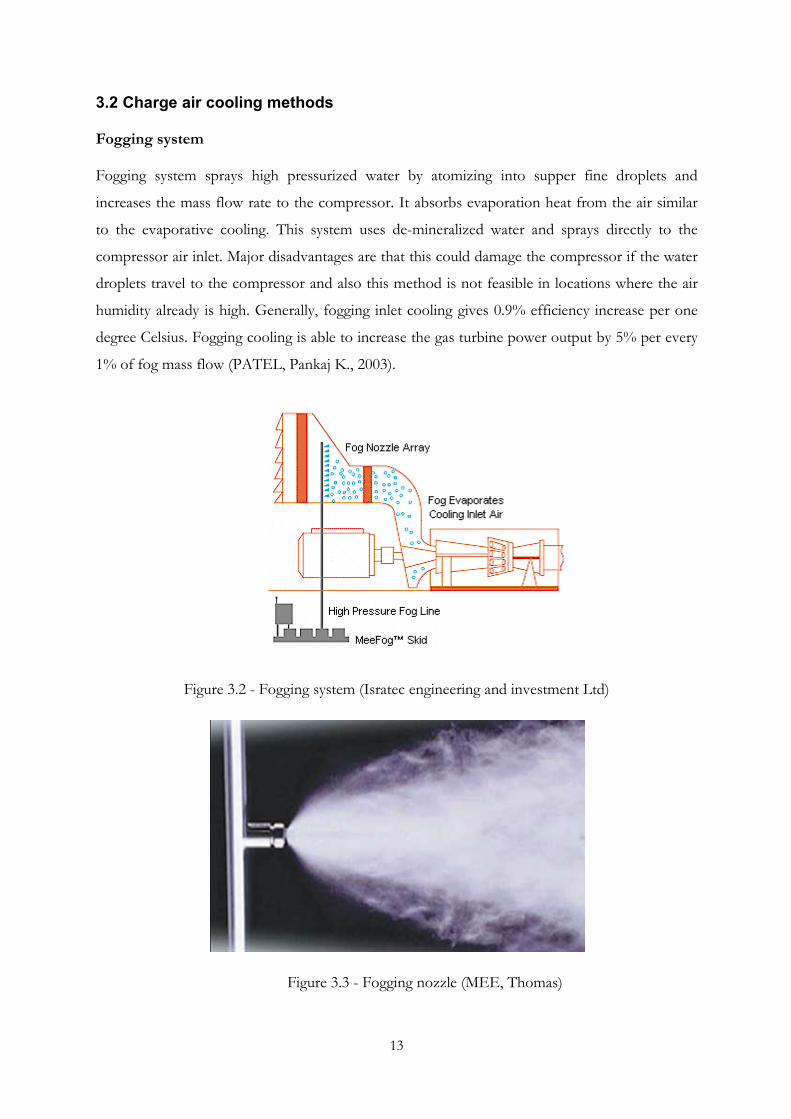
Fogging system sprays high pressurized water by atomizing into supper fine droplets and
increases the mass flow rate to the compressor. It absorbs evaporation heat from the air similar
to the evaporative cooling. This system uses de-mineralized water and sprays directly to the
compressor air inlet. Major disadvantages are that this could damage the compressor if the water
droplets travel to the compressor and also this method is not feasible in locations where the air
humidity already is high. Generally, fogging inlet cooling gives 0.9% efficiency increase per one
degree Celsius. Fogging cooling is able to increase the gas turbine power output by 5% per every
1% of fog mass flow (PATEL, Pankaj K., 2003).
Figure 3.2 - Fogging system (Isratec engineering and investment Ltd)
Figure 3.3 - Fogging nozzle (MEE, Thomas)
14
Evaporative cooler
Evaporative cooling is similar to the fogging system, however, water is not directly injected to the
compressor inlet. Instead, inlet air is allowed to travel through a shower of water and the latent
heat of water evaporation absorbs energy from the inlet air. Excess water is drained away from
the system. This is very low cost method of inlet air cooling. But, the performance is limited by
the wet bulb temperature reading (RH value) of the site, that is again limited by the relative
humidity of ambient air.
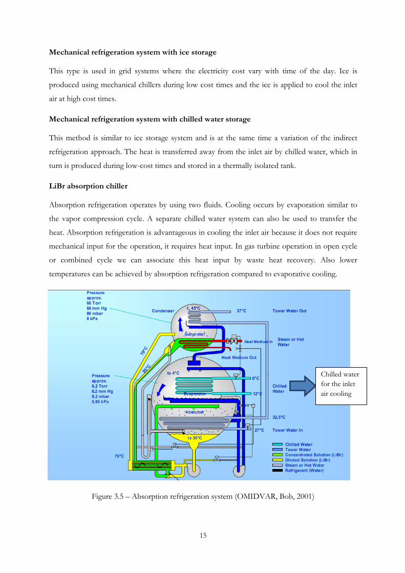
Mechanical refrigeration system (Direct type)
Refrigerant type chiller systems can be used directly to decrease the inlet air temperature using
vapor compression cycle. The inlet air directly is passed through the evaporator. By this method
it is possible to bring the inlet air to any desired value, for example the standard temperature of
150C (PATEL, Pankaj K., 2003). But it decreases the inlet air pressure and adversely affects the
overall output due to the comparatively large power consumption for cooling.
Figure 3.4 – Mechanical refrigeration system (OMIDVAR, Bob, 2001)
Mechanical refrigeration system (indirect type)
Indirect system uses chilled water as cooling media at the compressor inlet. The system
comprises a separate chiller system for inlet cooling.
15
Mechanical refrigeration system with ice storage
This type is used in grid systems where the electricity cost vary with time of the day. Ice is
produced using mechanical chillers during low cost times and the ice is applied to cool the inlet
air at high cost times.
Mechanical refrigeration system with chilled water storage
This method is similar to ice storage system and is at the same time a variation of the indirect
refrigeration approach. The heat is transferred away from the inlet air by chilled water, which in
turn is produced during low-cost times and stored in a thermally isolated tank.
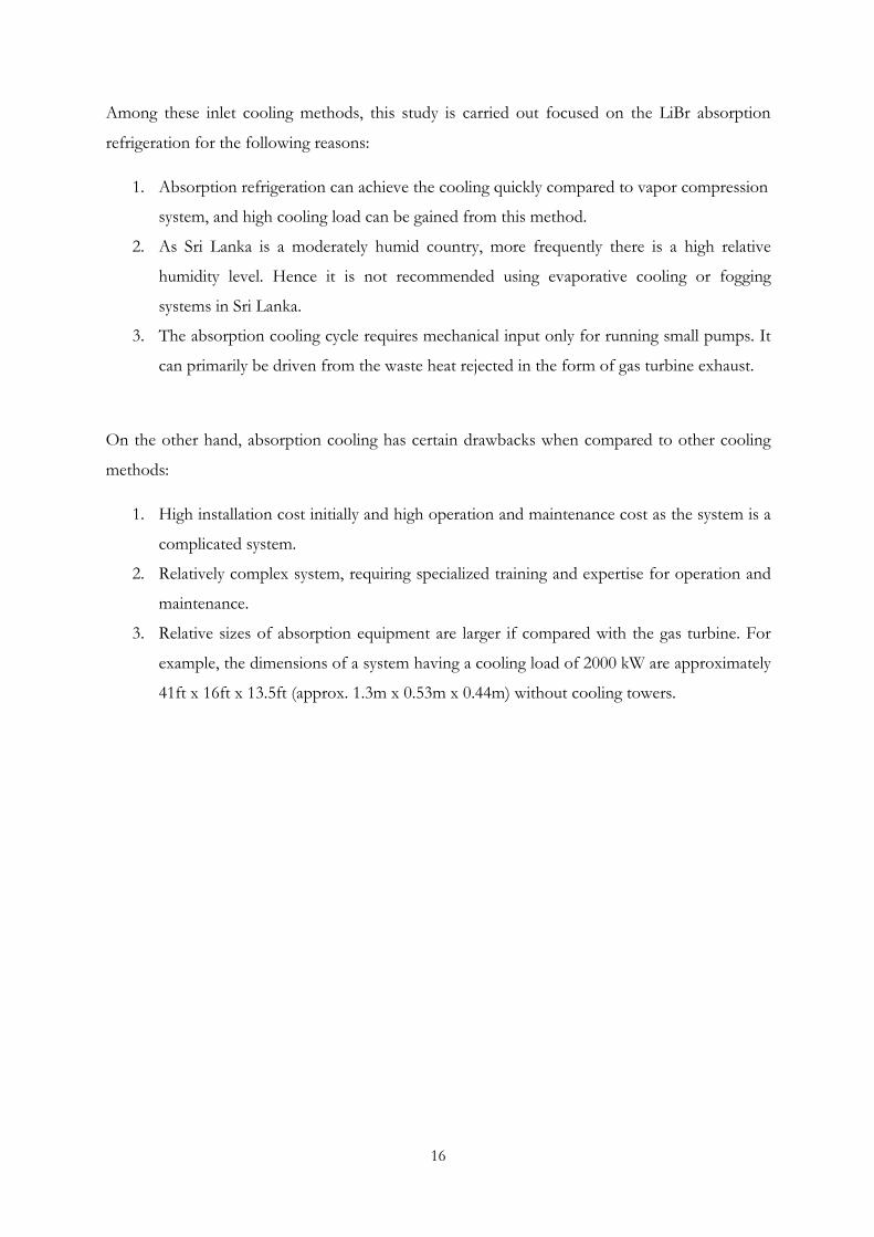
LiBr absorption chiller
Absorption refrigeration operates by using two fluids. Cooling occurs by evaporation similar to
the vapor compression cycle. A separate chilled water system can also be used to transfer the
heat. Absorption refrigeration is advantageous in cooling the inlet air because it does not require
mechanical input for the operation, it requires heat input. In gas turbine operation in open cycle
or combined cycle we can associate this heat input by waste heat recovery. Also lower
temperatures can be achieved by absorption refrigeration compared to evaporative cooling.
Figure 3.5 – Absorption refrigeration system (OMIDVAR, Bob, 2001)
Chilled water for the inlet air cooling
16
Among these inlet cooling methods, this study is carried out focused on the LiBr absorption
refrigeration for the following reasons:
1. Absorption refrigeration can achieve the cooling quickly compared to vapor compression
system, and high cooling load can be gained from this method.
2. As Sri Lanka is a moderately humid country, more frequently there is a high relative
humidity level. Hence it is not recommended using evaporative cooling or fogging
systems in Sri Lanka.
3. The absorption cooling cycle requires mechanical input only for running small pumps. It
can primarily be driven from the waste heat rejected in the form of gas turbine exhaust.
On the other hand, absorption cooling has certain drawbacks when compared to other cooling
methods:
1. High installation cost initially and high operation and maintenance cost as the system is a
complicated system.
2. Relatively complex system, requiring specialized training and expertise for operation and
maintenance.
3. Relative sizes of absorption equipment are larger if compared with the gas turbine. For
example, the dimensions of a system having a cooling load of 2000 kW are approximately
41ft x 16ft x 13.5ft (approx. 1.3m x 0.53m x 0.44m) without cooling towers.
17
4. Thermodynamic approach on the gas turbine and inlet cooling
Thermodynamic analysis in this chapter is a brief outline of the generalized gas turbine
performance, efficiency and its characteristics. Air-standard Brayton cycle is assumed for the
analysis of the thermodynamic processes.
4.1 Gas turbine performance and Brayton cycle
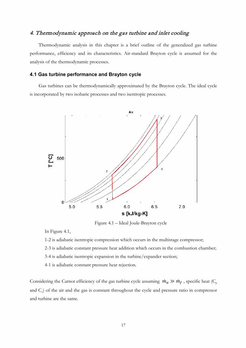
Gas turbines can be thermodynamically approximated by the Brayton cycle. The ideal cycle
is incorporated by two isobaric processes and two isentropic processes.
Figure 4.1 – Ideal Joule-Brayton cycle
In Figure 4.1,
1-2 is adiabatic isentropic compression which occurs in the multistage compressor;
2-3 is adiabatic constant pressure heat addition which occurs in the combustion chamber;
3-4 is adiabatic isentropic expansion in the turbine/expander section;
4-1 is adiabatic constant pressure heat rejection.
Considering the Carnot efficiency of the gas turbine cycle assuming �̇�𝑎 ≫ �̇�𝑓 , specific heat (Cp
and Cv) of the air and the gas is constant throughout the cycle and pressure ratio in compressor
and turbine are the same.
18
Power input to the compressor
𝑃𝑐 = �̇�𝑎𝑖𝑟 . (ℎ2 − ℎ1) … … … … … … … … … … … … … … … … … … … . . … … (4.1)
Turbine power output
𝑃𝑡 = �̇�𝑔𝑎𝑠. (ℎ3 − ℎ4) … … … … … … … … … … … … … … … … … . . … … … . . (4.2)
Net work output of the cycle (simple cycle)
𝑊𝑐𝑦𝑐 = 𝑊𝑡 −𝑊𝑐 … … … … … … … … … … … … … … … … … … … … … … … . . . … . . (4.3)
Energy added to the system
𝑄2,3 = 𝑚𝑓𝑥𝐿𝐻𝑉𝑓𝑢𝑒𝑙 = (�̇�𝑎 + �̇�𝑓)̇ ℎ3 − �̇�𝑎ℎ2 … … … … … . . … … … . … . . (4.4)
Thus, the thermal efficiency of the cycle is
𝜂 =𝑊𝑐𝑦𝑐
𝑄2,3… … … … … … … … … … … … … … … … … … … … … … … … … … … . . … . . (4.5)
Also, with the above mentioned assumptions, following expression gives the relationship of
efficiency with pressure ratio (EASTOP, T.D., 2002):
𝜂 = 1 − � 1𝑟𝑝�
𝛾−1𝛾 … … … … … … … … … … … … … … … … … … … … … … … … … … . (4.6)
Considering the real gas turbine cycle if efficiency in the compressor is ηc and efficiency of
the turbine (expander) is ηt then the relation for the cycle efficiency for the firing temperature Tf
is (BOYCE, Meherwan P., 2002):
η𝑐𝑦𝑐 =
⎣⎢⎢⎢⎢⎡
𝜂𝑡𝑇𝑓 − 𝑇𝑎𝑚𝑏𝑟𝑝
�𝛾−1𝛾 �
𝜂𝑐
𝑇𝑓 − 𝑇𝑎𝑚𝑏 − 𝑇𝑎𝑚𝑏 �𝑟𝑝
�𝛾−1𝛾 �−1
𝜂𝑐�⎦⎥⎥⎥⎥⎤
�1 −1
𝑟𝑝�𝛾−1𝛾 �
�… … … … … … … . . (4.7)
The most affecting factors for the gas turbine thermal efficiency are the compression ratio
of the compressor and the turbine inlet temperature (Gas turbine firing temperature). Gas
turbine thermal efficiency increases dramatically with the increase of compressor compression
ratio. However, it starts to decrease after a certain value of the compression ratio for the given
temperatures. Higher values of pressure ratios can decrease the operating range of the
compressor and it will be much more vulnerable to failures that could be caused by surges, dust
and sedimentations on the blades. Hence the values for the pressure ratio should be optimized
according for the application used.
19
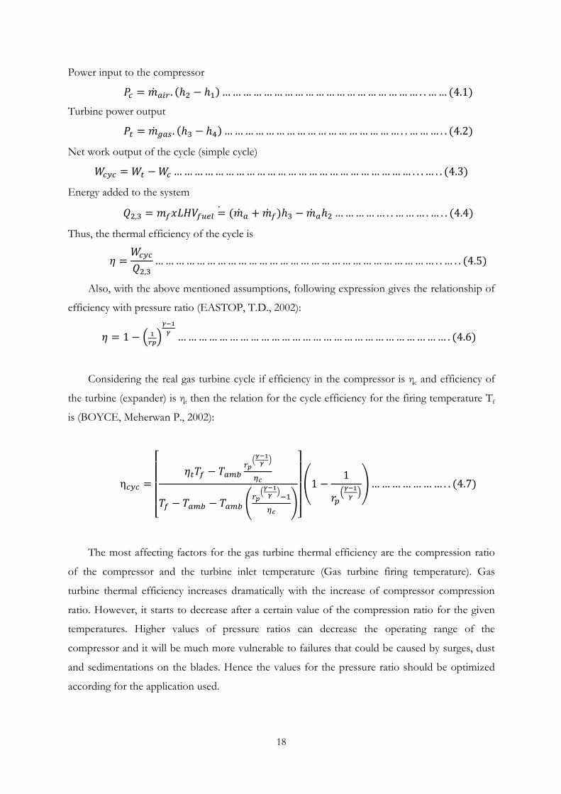
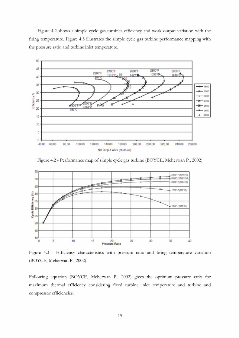
Figure 4.2 shows a simple cycle gas turbines efficiency and work output variation with the
firing temperature. Figure 4.3 illustrates the simple cycle gas turbine performance mapping with
the pressure ratio and turbine inlet temperature.
Figure 4.2 - Performance map of simple cycle gas turbine (BOYCE, Meherwan P., 2002)
Figure 4.3 - Efficiency characteristics with pressure ratio and firing temperature variation
(BOYCE, Meherwan P., 2002)
Following equation (BOYCE, Meherwan P., 2002) gives the optimum pressure ratio for
maximum thermal efficiency considering fixed turbine inlet temperature and turbine and
compressor efficiencies:
20
(𝑟𝑝)𝑒𝑜𝑝𝑡 =
� 1𝑇1𝑇3𝜂𝑡−𝑇1𝑇3+𝑇1
�𝑇1𝑇3𝜂𝑡 −
�(𝑇1𝑇3𝜂𝑡)2 − �𝑇1𝑇3𝜂𝑡 − 𝑇1𝑇3 + 𝑇12�(𝑇32𝜂𝑐𝜂𝑡 − 𝑇1𝑇3𝜂𝑡𝜂𝑐 + 𝑇1𝑇3𝜂𝑡)��
𝛾𝛾−1
… … … … . (4.8)
This optimum pressure ratio can be found for maximum work output with turbine section and
compressor section efficiency (BOYCE, Meherwan P., 2002).
(𝒓𝒑)𝑷𝒘𝒐𝒑𝒕 = �𝑇3𝜂𝑡𝜂𝑐
2𝑇1+
12�
𝛾𝛾−1
… … … … … … … … … … … … … … … … … … … … … (4.9)
Analyzing the two equations for the two pressure ratios (𝑟𝑝)𝑒𝑜𝑝𝑡 and (𝑟)𝑃𝑤𝑜𝑝𝑡 for the pressure
ratio for maximum efficiency is greater than the pressure ratio for the maximum work output, for
the same values of firing temperature and turbine and compressor efficiencies.
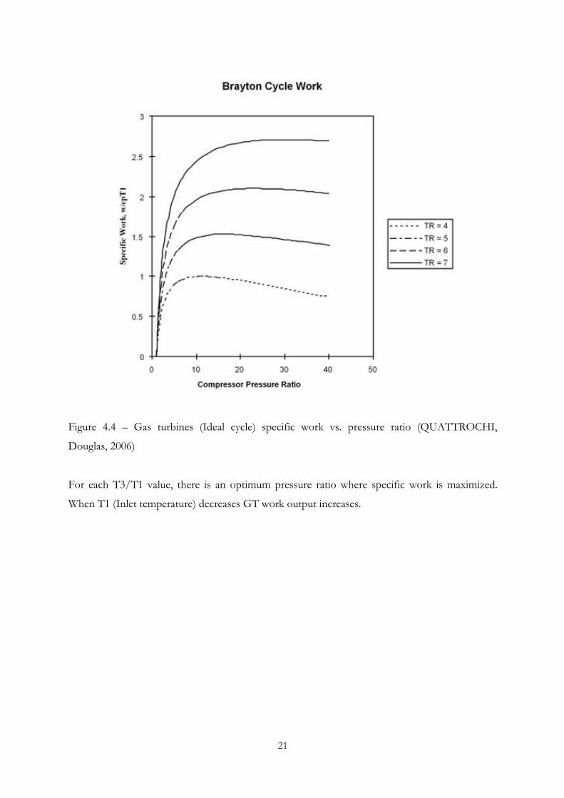
Figure 4.4 below presents the normalized specific work output for the air-standard Brayton cycle
as a function of compressor pressure ratio and of temperature increase ratio within the cycle. The
influence of compressor air inlet temperature (T1) on the cycle work output can also be derived
from the diagram.
21
Figure 4.4 – Gas turbines (Ideal cycle) specific work vs. pressure ratio (QUATTROCHI,
Douglas, 2006)
For each T3/T1 value, there is an optimum pressure ratio where specific work is maximized.
When T1 (Inlet temperature) decreases GT work output increases.
22
4.2 Cooling load estimation for gas turbine inlet cooling
To analyze the GT inlet cooling with absorption refrigeration, the cooling load is to be
calculated by referring to the actual online data taken from the Kelanitissa gas turbine unit No:05.
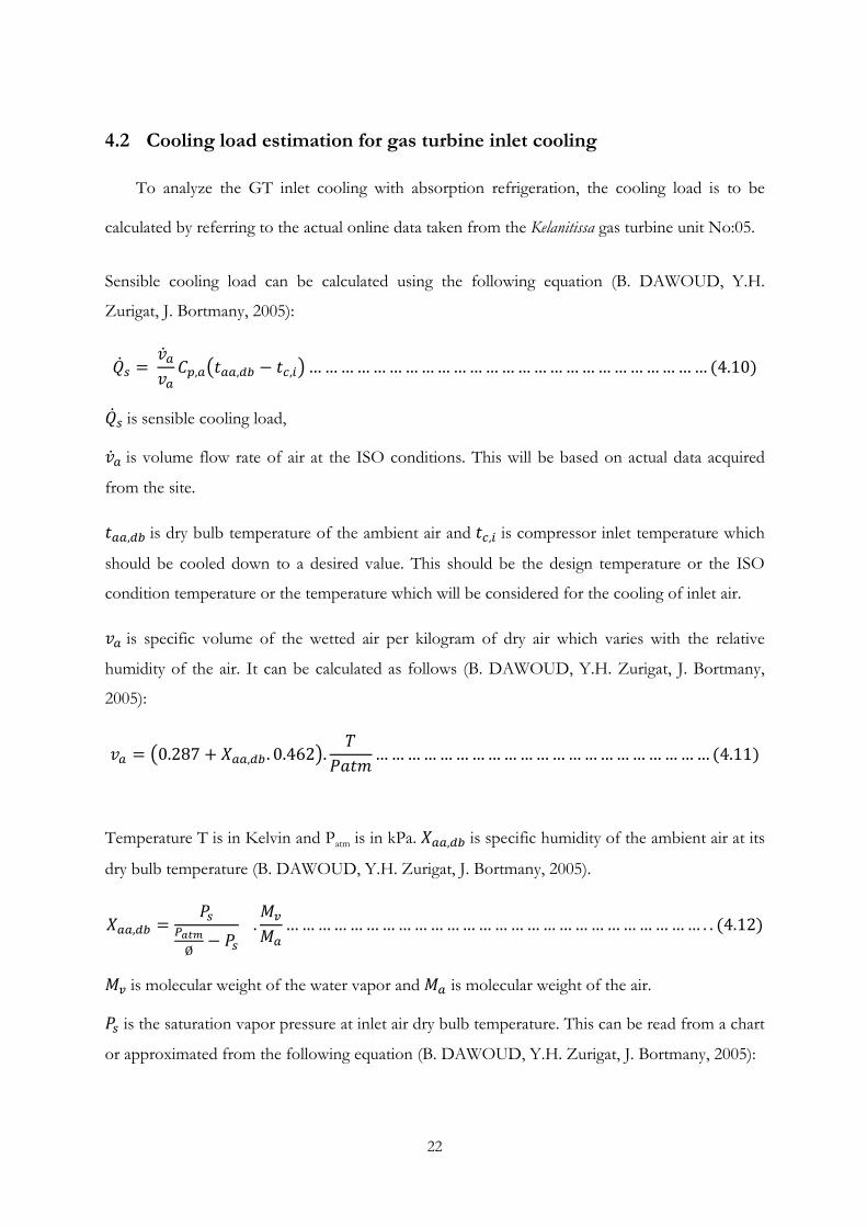
Sensible cooling load can be calculated using the following equation (B. DAWOUD, Y.H.
Zurigat, J. Bortmany, 2005):
�̇�𝑠 = �̇�𝑎𝑣𝑎𝐶𝑝,𝑎�𝑡𝑎𝑎,𝑑𝑏 − 𝑡𝑐,𝑖�… … … … … … … … … … … … … … … … … … … … … … … … … (4.10)
�̇�𝑠 is sensible cooling load,
�̇�𝑎 is volume flow rate of air at the ISO conditions. This will be based on actual data acquired
from the site.
𝑡𝑎𝑎,𝑑𝑏 is dry bulb temperature of the ambient air and 𝑡𝑐,𝑖 is compressor inlet temperature which
should be cooled down to a desired value. This should be the design temperature or the ISO
condition temperature or the temperature which will be considered for the cooling of inlet air.
𝑣𝑎 is specific volume of the wetted air per kilogram of dry air which varies with the relative
humidity of the air. It can be calculated as follows (B. DAWOUD, Y.H. Zurigat, J. Bortmany,
2005):
𝑣𝑎 = �0.287 + 𝑋𝑎𝑎,𝑑𝑏 . 0.462�.𝑇
𝑃𝑎𝑡𝑚… … … … … … … … … … … … … … … … … … … … … (4.11)
Temperature T is in Kelvin and Patm is in kPa. 𝑋𝑎𝑎,𝑑𝑏 is specific humidity of the ambient air at its
dry bulb temperature (B. DAWOUD, Y.H. Zurigat, J. Bortmany, 2005).
𝑋𝑎𝑎,𝑑𝑏 =𝑃𝑠
𝑃𝑎𝑡𝑚Ø
− 𝑃𝑠 .𝑀𝑣
𝑀𝑎… … … … … … … … … … … … … … … … … … … … … … … … … … . . (4.12)
𝑀𝑣 is molecular weight of the water vapor and 𝑀𝑎 is molecular weight of the air.
𝑃𝑠 is the saturation vapor pressure at inlet air dry bulb temperature. This can be read from a chart
or approximated from the following equation (B. DAWOUD, Y.H. Zurigat, J. Bortmany, 2005):
23
𝑃𝑠 = 22064. exp �−7.76451 �1 − 𝑇
647.14� + 1.45838 �
1 − 𝑇647.14
�1.5
− 2.7758 �1 − 𝑇
647.14�3
− 1.23303 �1 − 𝑇
647.14�6
/ �𝑇
647.14��… … … … … … … … … … … … … … … … … … … … … … … … . . (4.13)
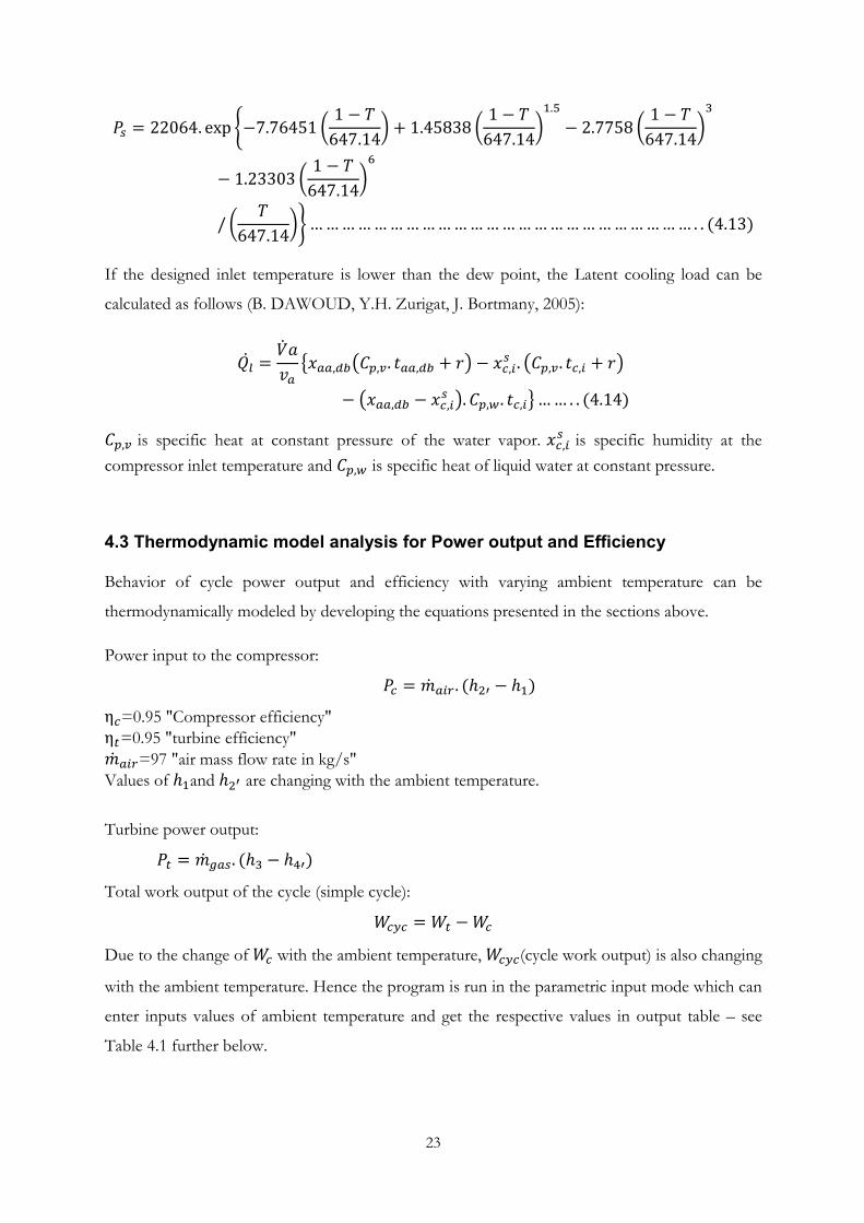
If the designed inlet temperature is lower than the dew point, the Latent cooling load can be
calculated as follows (B. DAWOUD, Y.H. Zurigat, J. Bortmany, 2005):
𝑄𝑙̇ =�̇�𝑎𝑣𝑎
�𝑥𝑎𝑎,𝑑𝑏�𝐶𝑝,𝑣. 𝑡𝑎𝑎,𝑑𝑏 + 𝑟� − 𝑥𝑐,𝑖𝑠 . �𝐶𝑝,𝑣. 𝑡𝑐,𝑖 + 𝑟�
− �𝑥𝑎𝑎,𝑑𝑏 − 𝑥𝑐,𝑖𝑠 �.𝐶𝑝,𝑤. 𝑡𝑐,𝑖�… … . . (4.14)
𝐶𝑝,𝑣 is specific heat at constant pressure of the water vapor. 𝑥𝑐,𝑖𝑠 is specific humidity at the
compressor inlet temperature and 𝐶𝑝,𝑤 is specific heat of liquid water at constant pressure.
4.3 Thermodynamic model analysis for Power output and Efficiency
Behavior of cycle power output and efficiency with varying ambient temperature can be
thermodynamically modeled by developing the equations presented in the sections above.
Power input to the compressor:
𝑃𝑐 = �̇�𝑎𝑖𝑟 . (ℎ2′ − ℎ1)
η𝑐=0.95 "Compressor efficiency" η𝑡=0.95 "turbine efficiency" �̇�𝑎𝑖𝑟=97 "air mass flow rate in kg/s" Values of ℎ1and ℎ2′ are changing with the ambient temperature.
Turbine power output:
𝑃𝑡 = �̇�𝑔𝑎𝑠. (ℎ3 − ℎ4′)
Total work output of the cycle (simple cycle):
𝑊𝑐𝑦𝑐 = 𝑊𝑡 −𝑊𝑐
Due to the change of 𝑊𝑐 with the ambient temperature, 𝑊𝑐𝑦𝑐(cycle work output) is also changing
with the ambient temperature. Hence the program is run in the parametric input mode which can
enter inputs values of ambient temperature and get the respective values in output table – see
Table 4.1 further below.
24
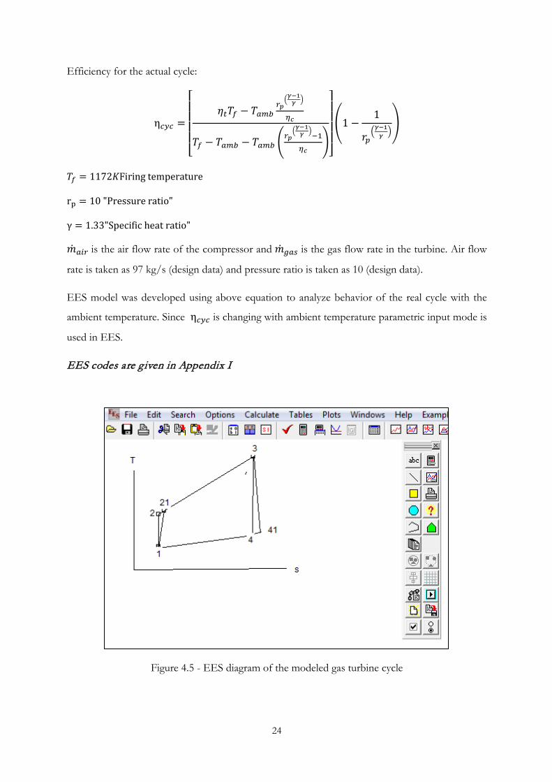
Efficiency for the actual cycle:
η𝑐𝑦𝑐 =
⎣⎢⎢⎢⎢⎡
𝜂𝑡𝑇𝑓 − 𝑇𝑎𝑚𝑏𝑟𝑝
�𝛾−1𝛾 �
𝜂𝑐
𝑇𝑓 − 𝑇𝑎𝑚𝑏 − 𝑇𝑎𝑚𝑏 �𝑟𝑝
�𝛾−1𝛾 �−1
𝜂𝑐�⎦⎥⎥⎥⎥⎤
�1 −1
𝑟𝑝�𝛾−1𝛾 �
�
𝑇𝑓 = 1172𝐾Firing temperature
rp = 10 "Pressure ratio"
γ = 1.33"Specific heat ratio"
�̇�𝑎𝑖𝑟 is the air flow rate of the compressor and �̇�𝑔𝑎𝑠 is the gas flow rate in the turbine. Air flow
rate is taken as 97 kg/s (design data) and pressure ratio is taken as 10 (design data).
EES model was developed using above equation to analyze behavior of the real cycle with the
ambient temperature. Since η𝑐𝑦𝑐 is changing with ambient temperature parametric input mode is
used in EES.
EES codes are g iven in Appendix I
Figure 4.5 - EES diagram of the modeled gas turbine cycle
25
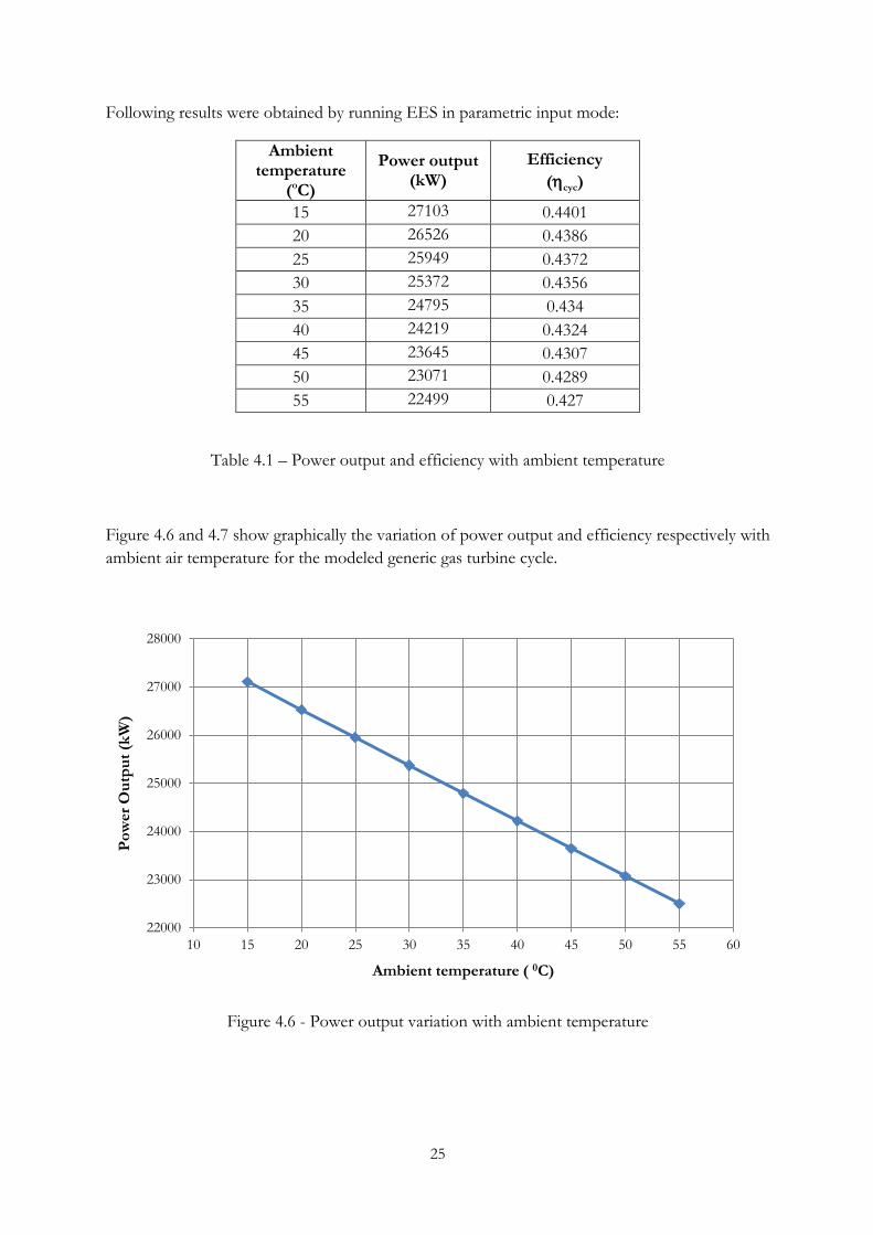
Following results were obtained by running EES in parametric input mode:
Ambient temperature
(oC)
Power output (kW)
Efficiency (ηcyc)
15 27103 0.4401 20 26526 0.4386 25 25949 0.4372 30 25372 0.4356 35 24795 0.434 40 24219 0.4324 45 23645 0.4307 50 23071 0.4289 55 22499 0.427
Table 4.1 – Power output and efficiency with ambient temperature
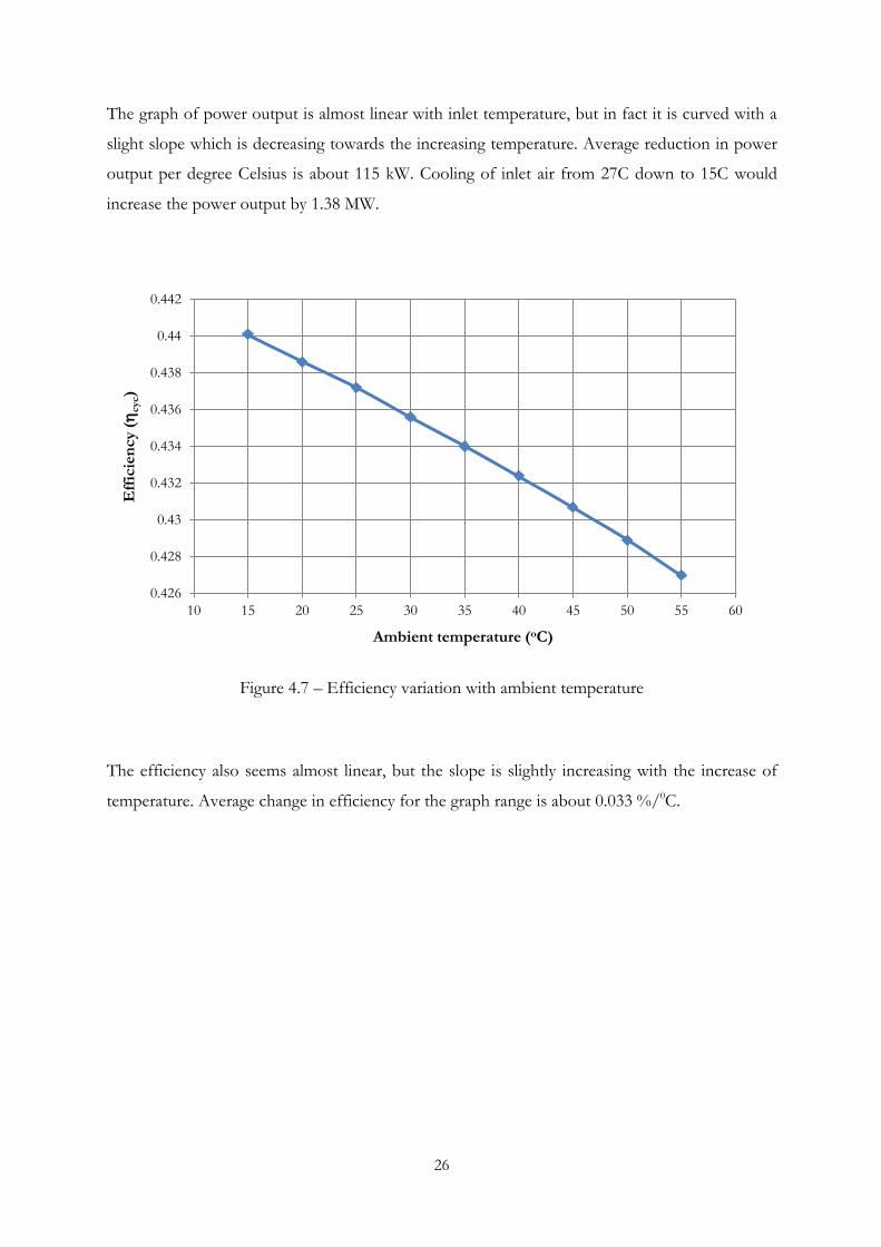
Figure 4.6 and 4.7 show graphically the variation of power output and efficiency respectively with ambient air temperature for the modeled generic gas turbine cycle.
Figure 4.6 - Power output variation with ambient temperature
22000
23000
24000
25000
26000
27000
28000
10 15 20 25 30 35 40 45 50 55 60
Pow
er O
utpu
t (kW
)
Ambient temperature ( 0C)
26
The graph of power output is almost linear with inlet temperature, but in fact it is curved with a
slight slope which is decreasing towards the increasing temperature. Average reduction in power
output per degree Celsius is about 115 kW. Cooling of inlet air from 27C down to 15C would
increase the power output by 1.38 MW.
Figure 4.7 – Efficiency variation with ambient temperature
The efficiency also seems almost linear, but the slope is slightly increasing with the increase of
temperature. Average change in efficiency for the graph range is about 0.033 %/0C.
0.426
0.428
0.43
0.432
0.434
0.436
0.438
0.44
0.442
10 15 20 25 30 35 40 45 50 55 60
Effi
cien
cy (η
cyc)
Ambient temperature (oC)
27
5. Analysis of data and results
This chapter presents the actual performance of the gas turbine in terms of efficiency, heat rate, active
power which were determined with the help of available data.
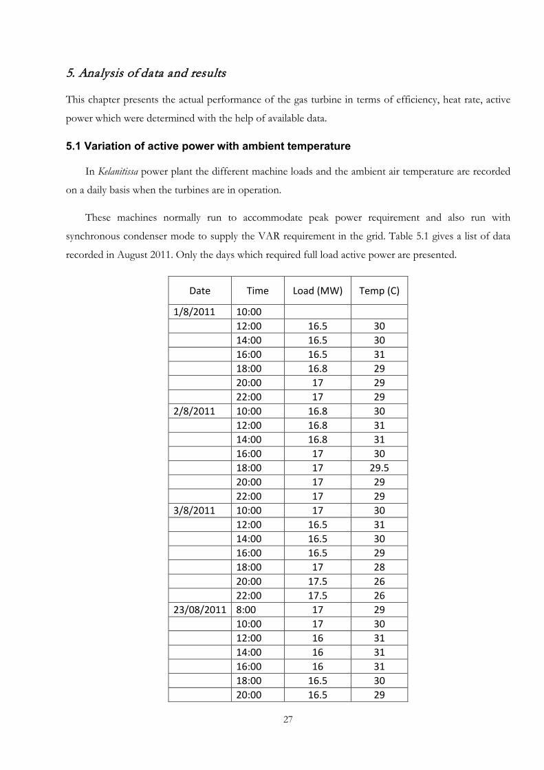
5.1 Variation of active power with ambient temperature
In Kelanitissa power plant the different machine loads and the ambient air temperature are recorded
on a daily basis when the turbines are in operation.
These machines normally run to accommodate peak power requirement and also run with
synchronous condenser mode to supply the VAR requirement in the grid. Table 5.1 gives a list of data
recorded in August 2011. Only the days which required full load active power are presented.
Date Time Load (MW) Temp (C)
1/8/2011 10:00 12:00 16.5 30 14:00 16.5 30 16:00 16.5 31 18:00 16.8 29 20:00 17 29 22:00 17 29 2/8/2011 10:00 16.8 30 12:00 16.8 31 14:00 16.8 31 16:00 17 30 18:00 17 29.5 20:00 17 29 22:00 17 29 3/8/2011 10:00 17 30 12:00 16.5 31 14:00 16.5 30 16:00 16.5 29 18:00 17 28 20:00 17.5 26 22:00 17.5 26 23/08/2011 8:00 17 29 10:00 17 30 12:00 16 31 14:00 16 31 16:00 16 31 18:00 16.5 30 20:00 16.5 29
28
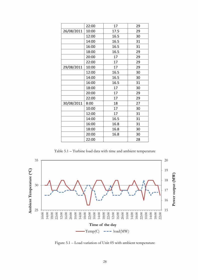
22:00 17 29 26/08/2011 10:00 17.5 29 12:00 16.5 30 14:00 16.5 31 16:00 16.5 31 18:00 16.5 29 20:00 17 29 22:00 17 29 29/08/2011 10:00 17 29 12:00 16.5 30 14:00 16.5 30 16:00 16.5 31 18:00 17 30 20:00 17 29 22:00 17 29 30/08/2011 8:00 18 27 10:00 17 30 12:00 17 31 14:00 16.5 31 16:00 16.8 31 18:00 16.8 30 20:00 16.8 30 22:00 28
Table 5.1 – Turbine load data with time and ambient temperature
Figure 5.1 – Load variation of Unit 05 with ambient temperature
15
16
17
18
19
20
25
30
35
10:0
014
:00
18:0
022
:00
12:0
016
:00
20:0
010
:00
14:0
018
:00
22:0
010
:00
14:0
018
:00
22:0
012
:00
16:0
020
:00
10:0
014
:00
18:0
022
:00
10:0
014
:00
18:0
022
:00
Pow
er o
utpu
t (M
W)
Am
bien
t Tem
pera
ture
(o C)
Time of the day
Temp(C) load(MW)
29
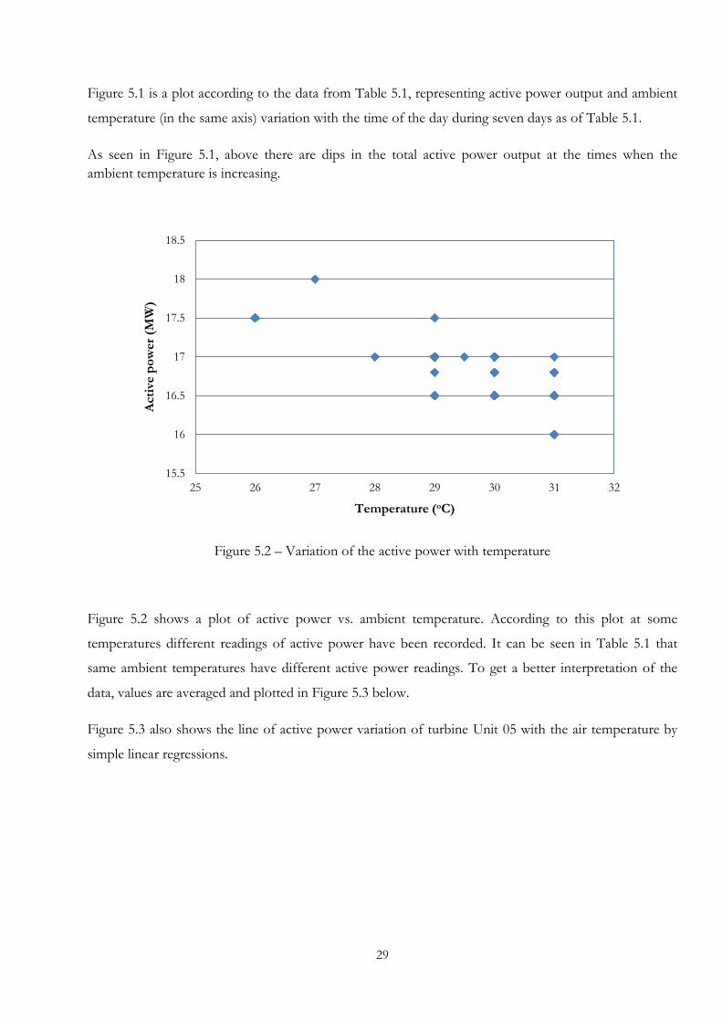
Figure 5.1 is a plot according to the data from Table 5.1, representing active power output and ambient
temperature (in the same axis) variation with the time of the day during seven days as of Table 5.1.
As seen in Figure 5.1, above there are dips in the total active power output at the times when the ambient temperature is increasing.
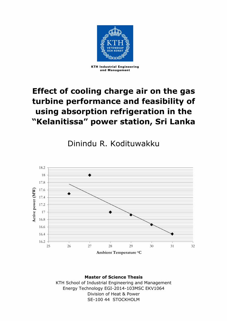
Figure 5.2 – Variation of the active power with temperature
Figure 5.2 shows a plot of active power vs. ambient temperature. According to this plot at some
temperatures different readings of active power have been recorded. It can be seen in Table 5.1 that
same ambient temperatures have different active power readings. To get a better interpretation of the
data, values are averaged and plotted in Figure 5.3 below.
Figure 5.3 also shows the line of active power variation of turbine Unit 05 with the air temperature by
simple linear regressions.
15.5
16
16.5
17
17.5
18
18.5
25 26 27 28 29 30 31 32
Act
ive
pow
er (M
W)
Temperature (oC)
30
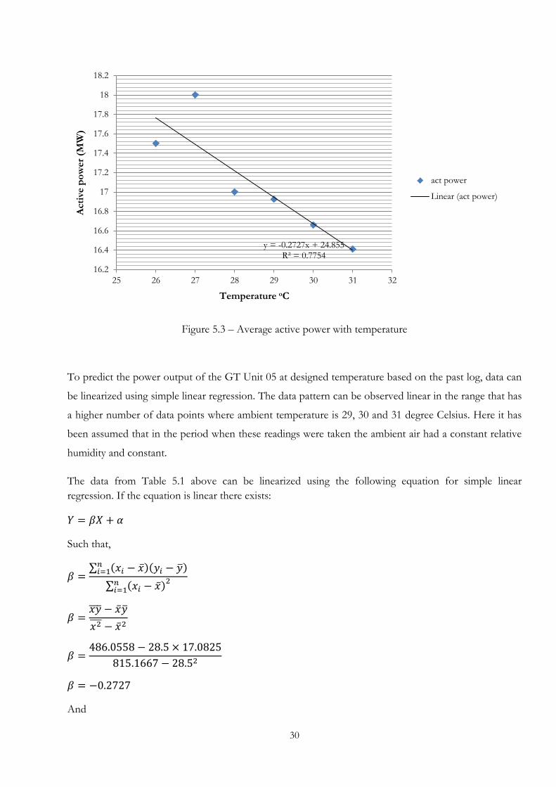
Figure 5.3 – Average active power with temperature
To predict the power output of the GT Unit 05 at designed temperature based on the past log, data can
be linearized using simple linear regression. The data pattern can be observed linear in the range that has
a higher number of data points where ambient temperature is 29, 30 and 31 degree Celsius. Here it has
been assumed that in the period when these readings were taken the ambient air had a constant relative
humidity and constant.
The data from Table 5.1 above can be linearized using the following equation for simple linear regression. If the equation is linear there exists:
𝑌 = 𝛽𝑋 + 𝛼
Such that,
𝛽 =∑ (𝑥𝑖 − �̅�)(𝑦𝑖 − 𝑦�)𝑛𝑖=1
∑ (𝑥𝑖 − �̅�)𝑛𝑖=1
2
𝛽 =𝑥𝑦��� − �̅�𝑦�𝑥2��� − �̅�2
𝛽 =486.0558 − 28.5 × 17.0825
815.1667 − 28.52
𝛽 = −0.2727
And
y = -0.2727x + 24.855 R² = 0.7754
16.2
16.4
16.6
16.8
17
17.2
17.4
17.6
17.8
18
18.2
25 26 27 28 29 30 31 32
Act
ive
pow
er (M
W)
Temperature oC
act power
Linear (act power)

31
𝛼 = 𝑌� − 𝛽𝑋�
𝛼 = 17.0825 − (−0.2727) × 28.5
𝛼 = 24.85
Hence the linearized equation is,
𝑌 = −0.2727𝑋 + 24.85
Machine active power is interpreted by Y and ambient temperature is interpreted by X.
Then to get active power at 150C, X is substituted by 15:
𝑌 = −0.2727(15) + 24.85
𝑌 = 20.7595
Hence the expected load at ambient temperature 150C is 20.76 MW.
5.2 Heat Rate test
Heat rate is a commonly used term for expressing the energy efficiency of the heat engines. Heat rate is
the fuel energy needed to generate a unit of electrical energy.
𝐻𝑒𝑎𝑡 𝑟𝑎𝑡𝑒 =𝑇𝑜𝑡𝑎𝑙 𝑒𝑛𝑒𝑟𝑔𝑦 𝑜𝑓 𝑐𝑜𝑛𝑠𝑢𝑚𝑒𝑑 𝑓𝑢𝑒𝑙 (𝑘𝐽/𝑘𝑔)𝐺𝑒𝑛𝑒𝑟𝑎𝑡𝑒𝑑 𝑒𝑙𝑒𝑐𝑡𝑟𝑖𝑐𝑎𝑙 𝑒𝑛𝑒𝑟𝑔𝑦 (𝑘𝑊ℎ)
A heat rate test had been carried-out for the Kelanitissa Power Station gas turbines on 21/05/2012 (see
Table 5.2 below). It has been done by the Public Utilities Commission of Sri Lanka, the organization
which is responsible for energy utilities in Sri Lanka.
32
Fuel Flow Meter Reading (Liters)
Generated Energy Meter Reading (MWh)
Auxiliary Energy Meter Reading (kWh)
Aux. Energy Meter Reading / Fin Fans (KWh)
Compres-sor Discharge Temp: (0C)
Exhaust Average Temp: (0C)
Initial Readings
Startup 32521106.00 682502 1072938 840691 - -
Synchronizing 32521269.00 682502 1072942 840693 - -
05 Minutes after Full Load 32521943.00 682503.5 1072943 840694 - - Running full load (17 MW) for 1 hour 32529735.00 682520.5 1072954 840712 328 492
Deloading Running Part Load (15 MW) for 1/2 hour 32533308.00 682528.3 1072959 840721 326 456
Running Part Load (12 MW) for 1/2 hour 32536435.00 682534.4 1072964 840729 321 420
Running Part Load (10 MW) for 1/2 hour 32539286.00 682539.5 1072970 840738 315 400
Shutdown
After Shutdown 32540104.00 682540.8 1072974 840741 - -
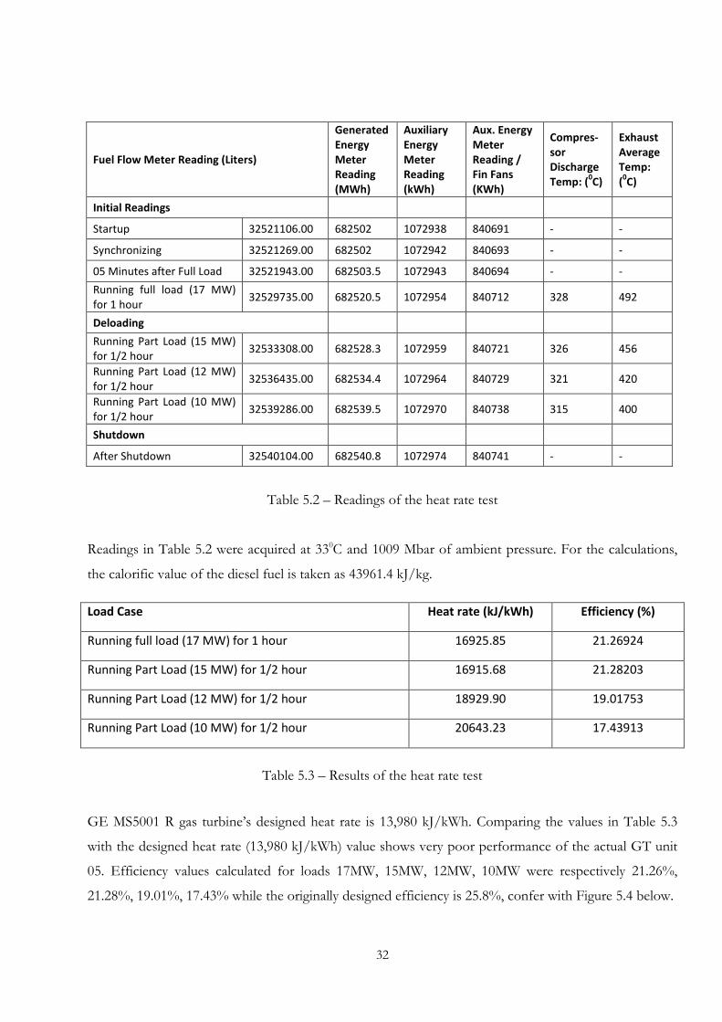
Table 5.2 – Readings of the heat rate test
Readings in Table 5.2 were acquired at 330C and 1009 Mbar of ambient pressure. For the calculations,
the calorific value of the diesel fuel is taken as 43961.4 kJ/kg.
Table 5.3 – Results of the heat rate test
GE MS5001 R gas turbine’s designed heat rate is 13,980 kJ/kWh. Comparing the values in Table 5.3
with the designed heat rate (13,980 kJ/kWh) value shows very poor performance of the actual GT unit
05. Efficiency values calculated for loads 17MW, 15MW, 12MW, 10MW were respectively 21.26%,
21.28%, 19.01%, 17.43% while the originally designed efficiency is 25.8%, confer with Figure 5.4 below.
Load Case Heat rate (kJ/kWh) Efficiency (%)
Running full load (17 MW) for 1 hour 16925.85 21.26924
Running Part Load (15 MW) for 1/2 hour 16915.68 21.28203
Running Part Load (12 MW) for 1/2 hour 18929.90 19.01753
Running Part Load (10 MW) for 1/2 hour 20643.23 17.43913
33
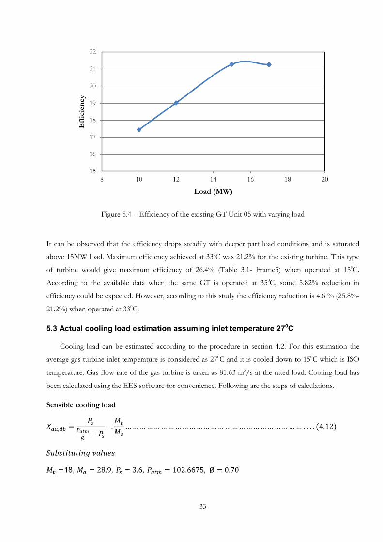
Figure 5.4 – Efficiency of the existing GT Unit 05 with varying load
It can be observed that the efficiency drops steadily with deeper part load conditions and is saturated
above 15MW load. Maximum efficiency achieved at 330C was 21.2% for the existing turbine. This type
of turbine would give maximum efficiency of 26.4% (Table 3.1- Frame5) when operated at 150C.
According to the available data when the same GT is operated at 350C, some 5.82% reduction in
efficiency could be expected. However, according to this study the efficiency reduction is 4.6 % (25.8%-
21.2%) when operated at 330C.
5.3 Actual cooling load estimation assuming inlet temperature 270C
Cooling load can be estimated according to the procedure in section 4.2. For this estimation the
average gas turbine inlet temperature is considered as 270C and it is cooled down to 150C which is ISO
temperature. Gas flow rate of the gas turbine is taken as 81.63 m3/s at the rated load. Cooling load has
been calculated using the EES software for convenience. Following are the steps of calculations.
Sensible cooling load
𝑋𝑎𝑎,𝑑𝑏 =𝑃𝑠
𝑃𝑎𝑡𝑚Ø
− 𝑃𝑠 .𝑀𝑣
𝑀𝑎… … … … … … … … … … … … … … … … … … … … … … … … … … . . (4.12)
𝑆𝑢𝑏𝑠𝑡𝑖𝑡𝑢𝑡𝑖𝑛𝑔 𝑣𝑎𝑙𝑢𝑒𝑠
𝑀𝑣 =18, 𝑀𝑎 = 28.9, 𝑃𝑠 = 3.6, 𝑃𝑎𝑡𝑚 = 102.6675, Ø = 0.70
15
16
17
18
19
20
21
22
8 10 12 14 16 18 20
Effi
cien
cy
Load (MW)
34
𝑋𝑎𝑎,𝑑𝑏 = 0.01567
𝑣𝑎 = �0.287 + 𝑋𝑎𝑎,𝑑𝑏 . 0.462�.𝑇
𝑃𝑎𝑡𝑚… … … … … … … … … … … … … … … … … … … … … (4.11)
𝑠𝑢𝑏𝑠𝑡𝑖𝑡𝑢𝑡𝑖𝑛𝑔 𝑇 = 300
𝑣𝑎 = 0.8598
�̇�𝑠 = �̇�𝑎𝑣𝑎𝐶𝑝,𝑎�𝑡𝑎𝑎,𝑑𝑏 − 𝑡𝑐,𝑖�… … … … … … … … … … … … … … … … … … … … … … … … … (4.10)
�̇�𝑎 = 81.63, 𝑡𝑐,𝑖 = 15, 𝐶𝑝,𝑎 = 1.004
�̇�𝑠 = 1143 𝑘𝑊
Latent Cooling load
𝑄𝑙̇ =�̇�𝑎𝑣𝑎
�𝑥𝑎𝑎,𝑑𝑏�𝐶𝑝,𝑣. 𝑡𝑎𝑎,𝑑𝑏 + 𝑟� − 𝑥𝑐,𝑖𝑠 . �𝐶𝑝,𝑣. 𝑡𝑐,𝑖 + 𝑟� − �𝑥𝑎𝑎,𝑑𝑏 − 𝑥𝑐,𝑖
𝑠 �.𝐶𝑝,𝑤. 𝑡𝑐,𝑖�… … . . (4.14)
𝑆𝑢𝑏𝑠𝑡𝑖𝑡𝑢𝑡𝑖𝑛𝑔 𝑣𝑎𝑙𝑢𝑒𝑠
𝐶𝑝,𝑣 = 1.866, 𝑡𝑎𝑎,𝑑𝑏 = 27, 𝑟 = 2500.8, 𝑥𝑐,𝑖𝑠 = 0.01049, 𝐶𝑝,𝑤 = 4.2
𝑄𝑙̇ = 1247 𝑘𝑊
Total cooling load 𝑄 = 𝑄𝑙̇ + �̇�𝑠 = 𝟐𝟑𝟗𝟏 𝒌𝑾
EES Codes are attached in appendix II
According to the calculations, the total cooling load is Q= 2391 kW (679.87 RT). This required energy is freely available in the hot exhaust gas behind the turbine outlet. In the present market there are few manufacturers who supply absorption chiller systems in commercial scale. Some of them are:
• Broad USA • Thermax Ldt. • Trane Inc. • York Intl.
These manufactures have compact designs to meet customers’ requirements which include chilled water
circulation system, cooling water circulation system with cooling towers, etc.
Broad USA is a company that supplies absorption chiller systems up to 3400 RT of cooling load, driven
by direct firing, steam or exhaust waste heat.
35
5.4 Economic Aspects of the project
Main focus of this section is to discuss about the economic feasibility of the project. Financial
calculations are based on the projected performance discussed in the previous chapter.
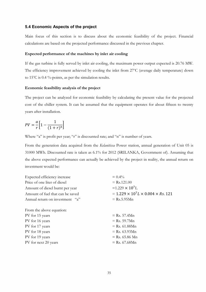
Expected performance of the machines by inlet air cooling
If the gas turbine is fully served by inlet air cooling, the maximum power output expected is 20.76 MW.
The efficiency improvement achieved by cooling the inlet from 27oC (average daily temperature) down
to 15oC is 0.4 %-points, as per the simulation results.
Economic feasibility analysis of the project
The project can be analyzed for economic feasibility by calculating the present value for the projected
cost of the chiller system. It can be assumed that the equipment operates for about fifteen to twenty
years after installation.
𝑃𝑉 =𝑎𝑟�1 −
1(1 + 𝑟)𝑛
�
Where “a” is profit per year; “r” is discounted rate; and “n” is number of years.
From the generation data acquired from the Kelanitissa Power station, annual generation of Unit 05 is
31000 MWh. Discounted rate is taken as 6.1% for 2012 (SRILANKA, Government of). Assuming that
the above expected performance can actually be achieved by the project in reality, the annual return on
investment would be:
Expected efficiency increase = 0.4% Price of one liter of diesel = Rs.121.00 Amount of diesel burnt per year =1.229 × 10⁷L Amount of fuel that can be saved = 1.229 × 107𝐿 × 0.004 × 𝑅𝑠. 121 Annual return on investment “a” = Rs.5.95Mn From the above equation: PV for 15 years = Rs. 57.4Mn PV for 16 years = Rs. 59.7Mn PV for 17 years = Rs. 61.88Mn PV for 18 years = Rs. 63.93Mn PV for 19 years = Rs. 65.86 Mn PV for next 20 years = Rs. 67.68Mn
36
Project cost estimation
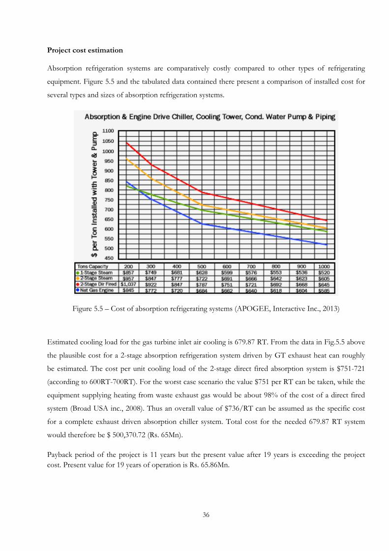
Absorption refrigeration systems are comparatively costly compared to other types of refrigerating
equipment. Figure 5.5 and the tabulated data contained there present a comparison of installed cost for
several types and sizes of absorption refrigeration systems.
Figure 5.5 – Cost of absorption refrigerating systems (APOGEE, Interactive Inc., 2013)
Estimated cooling load for the gas turbine inlet air cooling is 679.87 RT. From the data in Fig.5.5 above
the plausible cost for a 2-stage absorption refrigeration system driven by GT exhaust heat can roughly
be estimated. The cost per unit cooling load of the 2-stage direct fired absorption system is $751-721
(according to 600RT-700RT). For the worst case scenario the value $751 per RT can be taken, while the
equipment supplying heating from waste exhaust gas would be about 98% of the cost of a direct fired
system (Broad USA inc., 2008). Thus an overall value of $736/RT can be assumed as the specific cost
for a complete exhaust driven absorption chiller system. Total cost for the needed 679.87 RT system
would therefore be $ 500,370.72 (Rs. 65Mn).
Payback period of the project is 11 years but the present value after 19 years is exceeding the project cost. Present value for 19 years of operation is Rs. 65.86Mn.
37
5.5 System Design
This section focuses on some overall aspects of system design, in particular the extraction of energy
from the GT exhaust gas, the practical use of commercial absorption refrigeration components, and the
air cooling heat exchanger at the compressor inlet. The main steps of the design procedure are:
1. Selecting suitable products and manufacturers for an absorption chiller driven by exhaust gas; 2. Design of a heat exchanger for cooling the air at the inlet of the compressor; 3. Design of a hot gas inlet to the absorption refrigeration system.
Exhaust flue gas conditions of the Kelanitissa GT
GT exhaust mass flow rate is about 98.2 kg/s and the rated exhaust temperature is 513 0C. Volume flow rate of the exhaust gas is 167.2 m3 .
Total heat content (also represented by the theoretical exergy potential) of the exhaust gas waste heat flow can be calculated by the enthalpy drop down to ambient temperature:
�̇� = �̇�𝑔𝑎𝑠. (ℎ4 − ℎ1)
�̇� = 98.2 × (600.1 − 300.6)
�̇� = 29,410.9 𝑘𝑊
Selection of the Absorption refrigerating system
There are several established companies in the world which manufacture and supply absorption
refrigeration systems; they have already been presented in chapter 4.3 above. The further discussion here
is focusing on the products from the manufacturer Broad Inc. from USA. Among the product range of
Broad Inc., a suitable system can be selected and applied for GT inlet cooling.
Maximum cooling load required to bring the ambient temperature from an average of 27oC and
typical air humidity for the region, down to 15oC, is 2391 kW (679.87 RT). Necessary heating power
input to the chiller disregarding heat losses and system efficiency is therefore 2391 kW (or somewhat
above that value in practice), while the available energy rate in the GT exhaust gas flow is a massive
29,410.9 kW hence completely able to satisfy the requirement as per the energy balance. However, the
absorption chiller system requires the heating agent to have temperature levels according to
manufacturer’s specifications. To cover a cooling load of 2391 kW, a two-stage absorption refrigeration
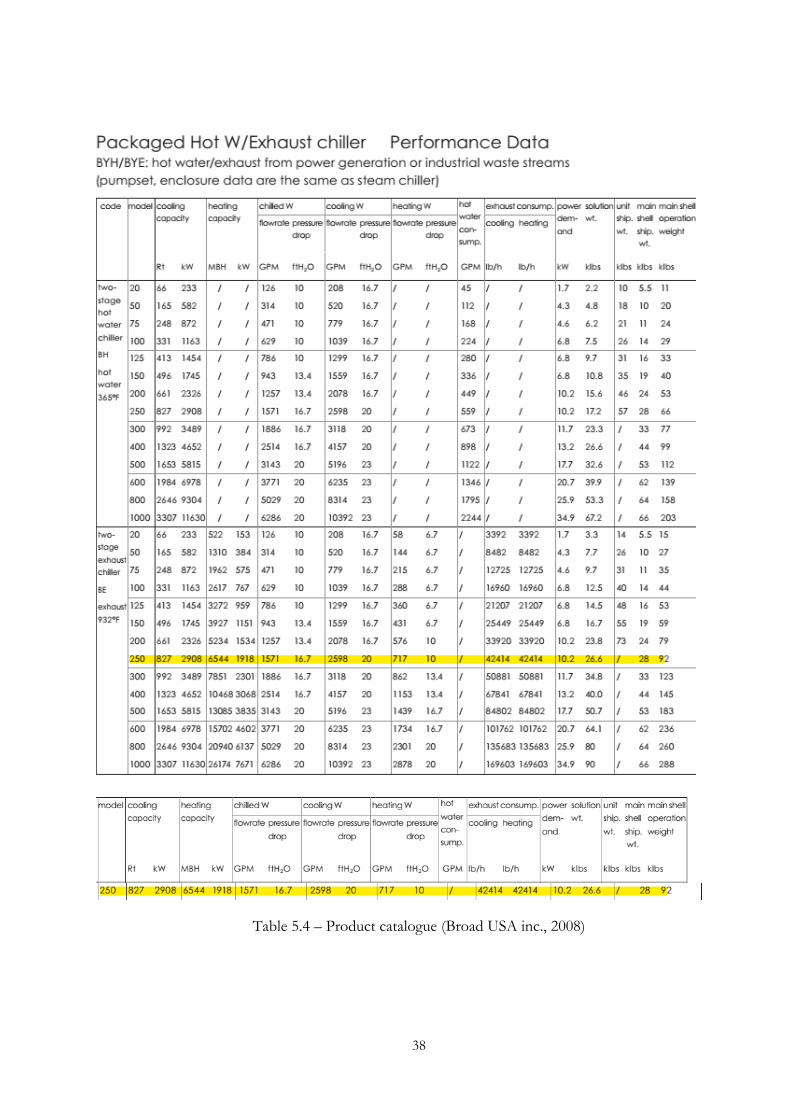
system should be utilized. The BYE250X absorption system by Broad Inc. is the chiller that can achieve
the cooling capacity required for the GT inlet cooling project, confer with Table 5.4.
38
Table 5.4 – Product catalogue (Broad USA inc., 2008)
39
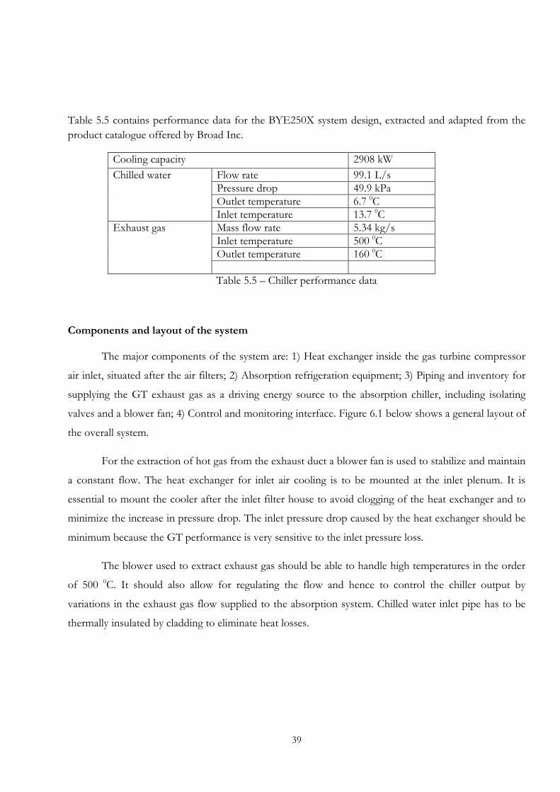
Table 5.5 contains performance data for the BYE250X system design, extracted and adapted from the product catalogue offered by Broad Inc.
Cooling capacity 2908 kW Chilled water Flow rate 99.1 L/s
Pressure drop 49.9 kPa Outlet temperature 6.7 0C Inlet temperature 13.7 0C
Exhaust gas Mass flow rate 5.34 kg/s Inlet temperature 500 0C Outlet temperature 160 0C Table 5.5 – Chiller performance data
Components and layout of the system
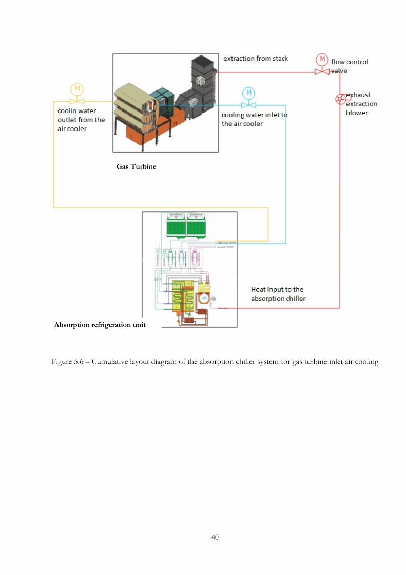
The major components of the system are: 1) Heat exchanger inside the gas turbine compressor
air inlet, situated after the air filters; 2) Absorption refrigeration equipment; 3) Piping and inventory for
supplying the GT exhaust gas as a driving energy source to the absorption chiller, including isolating
valves and a blower fan; 4) Control and monitoring interface. Figure 6.1 below shows a general layout of
the overall system.
For the extraction of hot gas from the exhaust duct a blower fan is used to stabilize and maintain
a constant flow. The heat exchanger for inlet air cooling is to be mounted at the inlet plenum. It is
essential to mount the cooler after the inlet filter house to avoid clogging of the heat exchanger and to
minimize the increase in pressure drop. The inlet pressure drop caused by the heat exchanger should be
minimum because the GT performance is very sensitive to the inlet pressure loss.
The blower used to extract exhaust gas should be able to handle high temperatures in the order
of 500 0C. It should also allow for regulating the flow and hence to control the chiller output by
variations in the exhaust gas flow supplied to the absorption system. Chilled water inlet pipe has to be
thermally insulated by cladding to eliminate heat losses.
40
Figure 5.6 – Cumulative layout diagram of the absorption chiller system for gas turbine inlet air cooling
Absorption refrigeration unit
Gas Turbine
41
6. Concluding Remarks
6.1 Power Output
Efficiency and power output are the key indexes of measuring gas turbine performance and
its variation with the fluctuations of inlet air temperature. Normally, gas turbine power output
and efficiency increase when the inlet air temperature is decreasing.
The power required to drive the compressor decreases with the decrease of ambient
temperature. In the T-S diagram it can be seen that the gap between two constant pressure lines
reduces with the decreasing temperature. Hence the power load in the compressor decreases with
the decrease of ambient temperature. For the Kelanitissa gas turbine, the actual power output
increase is about 272.7 kW per 1oC reduction of air temperature. This is about 22.3% increase.
The corresponding theoretical value for a generic gas turbine is 115.1 kW per 1oC reduction. It
should be noted that, when calculating the theoretical power output in this study the possible
variation of heat losses was neglected, considering them as constant with the change of inlet air
temperature, hence it would not affect the final result in the comparison of performance.
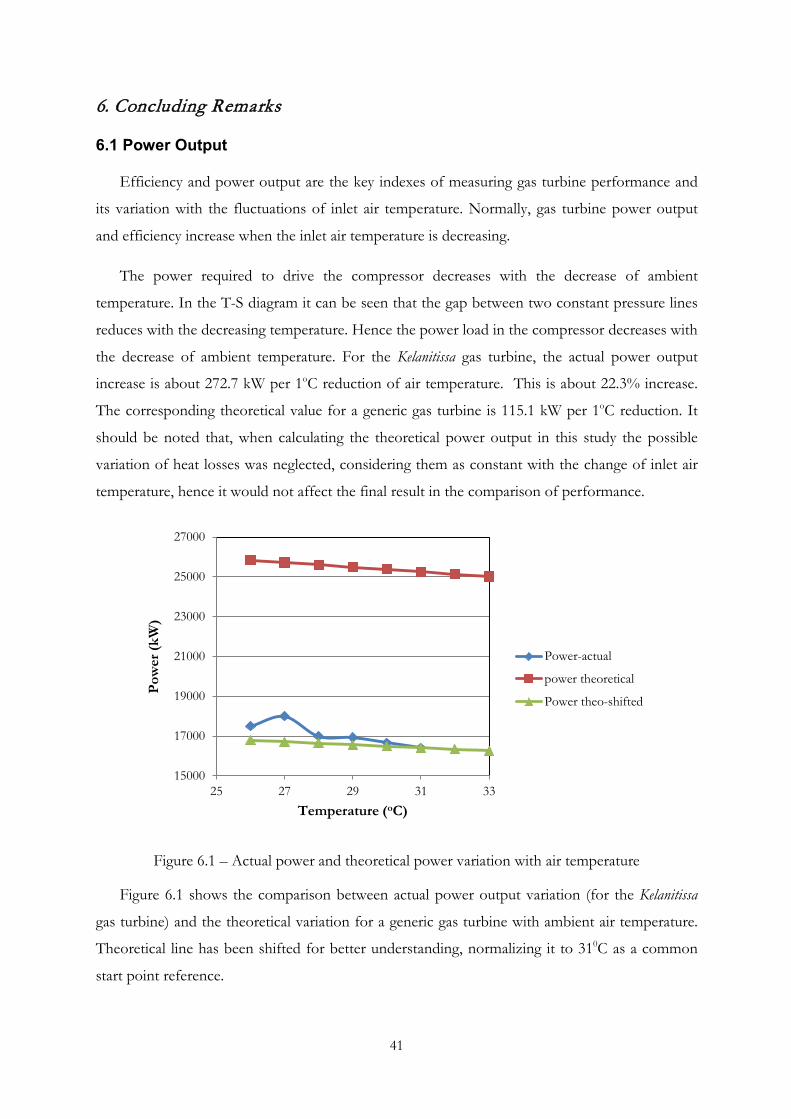
Figure 6.1 – Actual power and theoretical power variation with air temperature
Figure 6.1 shows the comparison between actual power output variation (for the Kelanitissa
gas turbine) and the theoretical variation for a generic gas turbine with ambient air temperature.
Theoretical line has been shifted for better understanding, normalizing it to 310C as a common
start point reference.
15000
17000
19000
21000
23000
25000
27000
25 27 29 31 33
Pow
er (k
W)
Temperature (oC)
Power-actual
power theoretical
Power theo-shifted
42
It can be clearly noticed that the actual power responds to a temperature change more than
the theoretically derived power variation. This difference could be due to the increase of
mechanical losses with the increase of temperature. Most probably it could be the heat loss which
is higher when the temperature is higher, causing the observed difference.
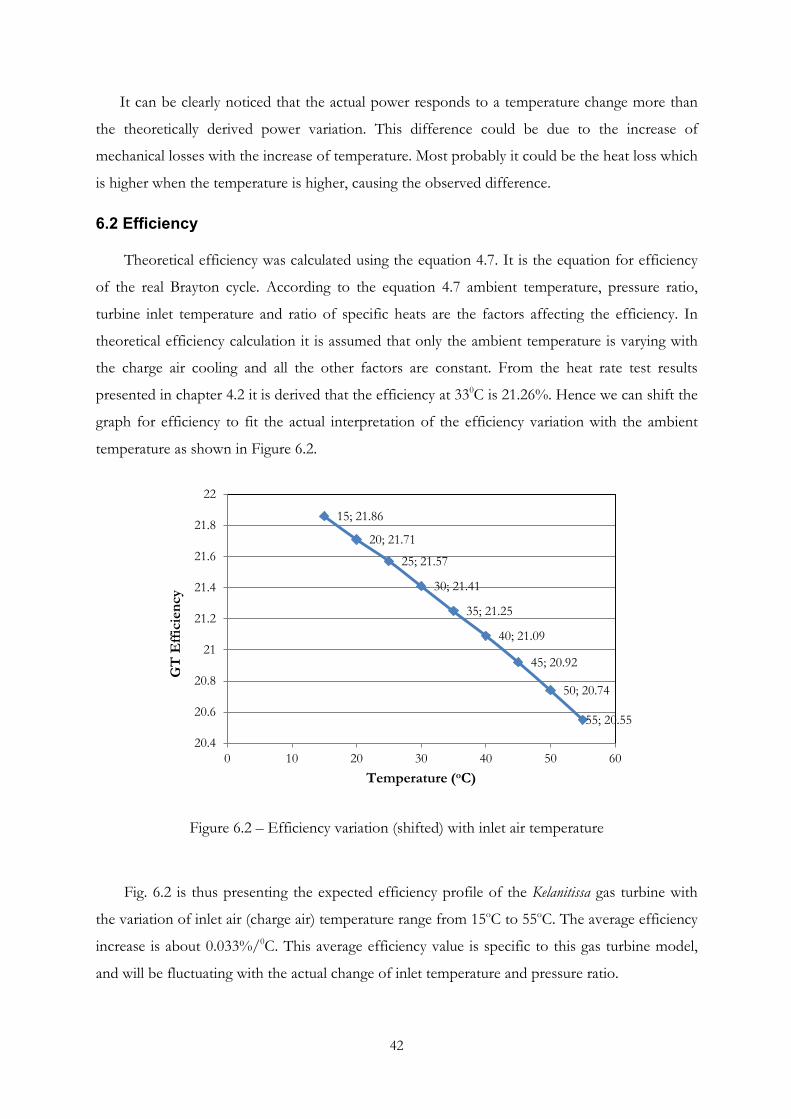
6.2 Efficiency
Theoretical efficiency was calculated using the equation 4.7. It is the equation for efficiency
of the real Brayton cycle. According to the equation 4.7 ambient temperature, pressure ratio,
turbine inlet temperature and ratio of specific heats are the factors affecting the efficiency. In
theoretical efficiency calculation it is assumed that only the ambient temperature is varying with
the charge air cooling and all the other factors are constant. From the heat rate test results
presented in chapter 4.2 it is derived that the efficiency at 330C is 21.26%. Hence we can shift the
graph for efficiency to fit the actual interpretation of the efficiency variation with the ambient
temperature as shown in Figure 6.2.
Figure 6.2 – Efficiency variation (shifted) with inlet air temperature
Fig. 6.2 is thus presenting the expected efficiency profile of the Kelanitissa gas turbine with
the variation of inlet air (charge air) temperature range from 15oC to 55oC. The average efficiency
increase is about 0.033%/0C. This average efficiency value is specific to this gas turbine model,
and will be fluctuating with the actual change of inlet temperature and pressure ratio.
15; 21.86
20; 21.71
25; 21.57
30; 21.41
35; 21.25
40; 21.09
45; 20.92
50; 20.74
55; 20.55
20.4
20.6
20.8
21
21.2
21.4
21.6
21.8
22
0 10 20 30 40 50 60
GT
Effi
cien
cy
Temperature (oC)
43
According to above Figures 6.1 and 6.2, the Kelanitissa gas turbine can reach up to 20.76 MW
power output and 21.86% efficiency maximum at 15oC of inlet air temperature, which is the
design temperature. The design performance indexes according to the manufacturer are 25.8% of
efficiency and 22.4MW power output. This major difference between the original performance
and the present performance is due to aging of the machine after nearly 30 years of operation.
6.3 Feasibility
According to chapter 5, 27oC is the average air temperature in Colombo year-round, and
bringing it down to ISO value of 150C gives Rs.5.9Mn of annual savings for the Kelanitissa gas
turbine Unit 05 at the established operational hours. This saving is only from the decreased
amount of fuel due to efficiency improvement. A value or measurement for economic return due
to the increase of active power output is not considered in the financial benefits of the project.
The annual power generation by the Kelanitissa plant can be increased by more than 20%. If the
inlet cooling is to be done by absorption refrigeration, the capital cost for a 600RT-700RT
system would be about Rs.65Mn ($500,370).
Direct payback for this system only by fuel savings is about eleven years (assuming constant
fuel prices as per 2013), but the benefit from power increase should also be considered in the
actual assessment of the practical feasibility if the additionally produced power can be sold to the
grid at the same conditions.
6.4 Future developments
Further studies can be done on this project to increase the accuracy of feasibility assessment
and to enhance the economic benefits. One option is to cool the inlet air for all five gas turbines
installed at the Kelanitissa power station by using exhaust gas from one gas turbine. This method
can keep cost down while achieving higher economic feasibility. It will require a chiller system
with larger cooling capacity which should be enough to cool the air for all the five gas turbines in
the power station. The exhaust gas from a single turbine does have the energy content to deliver
such large cooling load, however, that particular machine should be kept operating with priority
in order to supply precooled air to all other operating turbines at any particular moment. Again,
the overall increase of power production for the entire plant should also be valorized for the
financial benefits according to the actual operational hours for each of the available gas turbines
in the plant.

44
If the Kelanitissa power plant utilized inlet cooling from the beginning of its commercial life,
the past 30 years of operation would have saved a lot of money and energy, approximately at a
present value of Rs.81Mn. Waste heat can be used in many ways to optimize the use of energy;
extending the proposed chiller plant into a combined district cooling and/or heating unit which
could provide district cooling energy for commercial users in Colombo. A proper estimation of
the capital cost for such a project, however, is outside the scope of this study.
Open cycle gas turbine operation is normally omitted in modern power generating systems.
Still, there are many cases around the world where old or new gas turbines are utilized in open-
cycle mode for back-up or peak loads, or for various industrial drives in hot climates which
cumulatively present an enormous potential for efficiency improvement and fuel savings, with
the consequent benefit of an immediate decrease of the environmental footprint for these
installations. District cooling/heating systems are not an option in some locations, while the
utilization of exhaust gas heat for inlet air cooling could generally be applied anywhere in hot
climate zones. Deliverables of this study may be able to help optimizing the operation and the
environmental performance of such existing open cycle gas turbine plants.
45
References
(NLR), National Aerospace Labrotory. 2013. Gas turbine Simulation Program (GSP). [online].
2001. Gas Turbine Inlet Air Cooling System, perf. Bob OMIDVAR. Australian Gas Turbine Confrence.
AL-TOBI, Is'haq. 2009. Performance Enhancement of Gas Turbines by Inlet Air Cooling. In: International Conference on Communication Computer and Power(ICCCP'09). Muscat, pp.165-170.
APOGEE, Interactive Inc. 2013. APOGEE Interactive Energy library. [online]. [Accessed 2013]. Available from World Wide Web: <http://smud.apogee.net/comsuite/content/ces/?utilid=s&id=1084>
B. DAWOUD, Y.H. Zurigat, J. Bortmany. 2004. Thermodynamic assessment of power requirements and impact of different gas-turbine inlet air cooling techniques at two different locations in Oman. Oman: www.sciencedirect.com.
BOYCE, Meherwan P. 2002. Gas Turbine Engineering Handbook. Texas: Butterworth-Heinemann.
Broad USA inc. [online]. Available from World Wide Web: <http://www.broadusa.com/>
DAIBER, Paul C. Performance and Reliability Improvement for the MS5001 Gas Turbines. Atlanta: GE Power systems.
EASTOP, T.D. 2002. Applied Thermodynamics for Engineering Technologists. Longman Group UK Ltd.
H COHEN, GFC Rogers, HIH Saravanamuttoo. 1995. GAS TURBINE THEORY. Harlow, England: Longman Group Ltd.
Isratec engineering and investment Ltd. [online]. [Accessed 1 Nov 2011]. Available from World Wide Web: <http://www.isratec.com/content.php?actions=show&id=3015&b=1>
JOAN CARLES BRUNO, Víctor Ortega-López, Alberto Coronas. 2008. Integration of absorption cooling systems into micro gas turbine trigeneration. Elsvier.
L. GAROOCI FARSHI, S. M. Seyed Mahmoudi & A. H. Mosafa. 2008. Improvement of simple and regenerative gas turbine using simple and ejector-absorption refrigeration. IUST International Journal of Engineering Science., pp.127-136.
MEE, Thomas. Power engineering. [online]. [Accessed 1 Nov 2011]. Available from World Wide Web: <http://www.power-eng.com/articles/print/volume-115/issue-8/departments/what-works/oregon-state-leeds-the-nation-in-energy-efficiency.html>
PATEL, Pankaj K. 2003. BETTER POWER GENERATION FROM GAS TURBINE. ATLANTA: ASME.
QUATTROCHI, Douglas. 2006. Thermodynamic and propulsion-brayton cycle. [online]. Available from World Wide Web: <http://web.mit.edu/16.unified/www/FALL/thermodynamics/notes/node28.html>

46
RAQUEL GARETA, Luis M. Romeo, Antonia Gil. 2001. Methodology for the economic evaluation of gas turbine air-cooling systems in combined cycle applications. Zaragoza (Spain): University of Zaragoza.
SRILANKA, Government of. Central Bank of Sri Lanka. [online]. Available from World Wide Web: <http://www.cbsl.gov.lk/htm/english/05_fss/fss.html>
THAMIR K. IBRAHIM, M. M. Rahman, Ahmed N. Abdalla. 2011. Improvement of gas turbine performance based on inlet air cooling systems. International Journal of Physical Sciences., pp. 620-627.

47
Appendix I
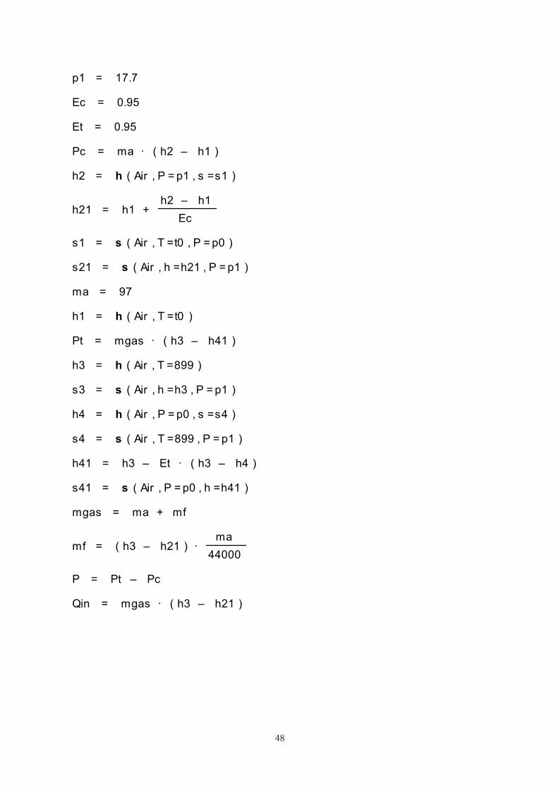
EES Equations for Power Output and Efficiency Calculation
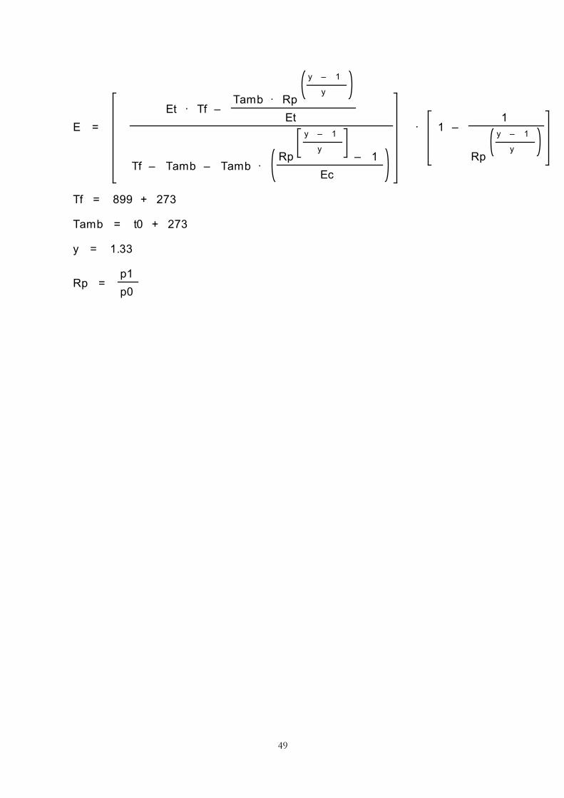
p0=1.04166"Inlet pressure in bar" p1=17.7"compressor discharge pressure" Ec=0.95"Compressor efficiency" Et=0.95"turbine efficiency" ma=97"air mass flow rate kg/s" Pc=ma*(h2-h1)*Ec"compressor power kw" h2=enthalpy(Air, p=p1, S=s1)"specific enthalpy in kJ/kg" h21= h1+((h2-h1)/Ec) s1=entropy(Air, T=t0, p=p0) s21=entropy(Air,h=h21,p=p1) h1=enthalpy(Air, T=t0) Pt= mgas*(h3-h41)*Et"turbine power" h3=enthalpy(Air,T=899) s3=entropy(Air,h=h3,p=p1) h4=enthalpy(Air,p=p0, S=s4) s4=entropy(Air, T=899, P=p1) h41=h3-Et*(h3-h4) s41=entropy(air, p=p0,h=h41) mgas=ma+mf"gas flow rate" mf=(h3-h21)*ma/44000"Fuel flow rate" P=Pt-Pc "power output" Qin=mgas*(h3-h21)"Total heat input" E=(( (Et*Tf-((Tamb*Rp^((y-1)/y))/Et))/(Tf-Tamb-Tamb*((Rp^((y-1)/y)-1)/Ec))))*(1-(1/Rp^((y-1)/y))) "Efficiency" Tf=899+273"firing temperature" Tamb=t0+273"ambient temperature" y=1.33"specific heat ratio" Rp=(p1/p0) "Pressure ratio" Formatted equations
p0 = 1.04166
48
p1 = 17.7
Ec = 0.95
Et = 0.95
Pc = ma · ( h2 – h1 )
h2 = h ( Air , P = p1 , s =s1 )
h21 = h1 + h2 – h1
Ec
s1 = s ( Air , T =t0 , P = p0 )
s21 = s ( Air , h =h21 , P = p1 )
ma = 97
h1 = h ( Air , T =t0 )
Pt = mgas · ( h3 – h41 )
h3 = h ( Air , T =899 )
s3 = s ( Air , h =h3 , P = p1 )
h4 = h ( Air , P = p0 , s =s4 )
s4 = s ( Air , T =899 , P = p1 )
h41 = h3 – Et · ( h3 – h4 )
s41 = s ( Air , P = p0 , h =h41 )
mgas = ma + mf
mf = ( h3 – h21 ) · ma
44000
P = Pt – Pc
Qin = mgas · ( h3 – h21 )
49
E = Et · Tf –
Tamb · Rp
y – 1
y
Et
Tf – Tamb – Tamb · Rp
y – 1
y – 1
Ec
· 1 – 1
Rp
y – 1
y
Tf = 899 + 273
Tamb = t0 + 273
y = 1.33
Rp = p1p0
50
Appendix II
EES Equations for Cooling Load Calculation
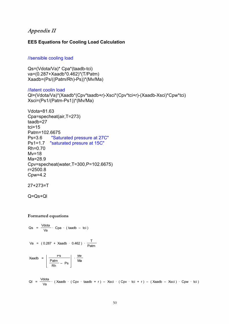
//sensible cooling load Qs=(Vdota/Va)* Cpa*(taadb-tci) va=(0.287+Xaadb*0.462)*(T/Patm) Xaadb=(Ps/((Patm/Rh)-Ps))*(Mv/Ma) //latent coolin load Ql=(Vdota/Va)*(Xaadb*(Cpv*taadb+r)-Xsci*(Cpv*tci+r)-(Xaadb-Xsci)*Cpw*tci) Xsci=(Ps1/(Patm-Ps1))*(Mv/Ma) Vdota=81.63 Cpa=specheat(air,T=273) taadb=27 tci=15 Patm=102.6675 Ps=3.6 "Saturated pressure at 27C" Ps1=1.7 "saturated presure at 15C" Rh=0.70 Mv=18 Ma=28.9 Cpv=specheat(water,T=300,P=102.6675) r=2500.8 Cpw=4.2 27+273=T Q=Qs+Ql
Formatted equations
Qs = Vdota
Va · Cpa · ( taadb – tci )
Va = ( 0.287 + Xaadb · 0.462 ) · T
Patm
Xaadb = Ps
PatmRh
– Ps ·
MvMa
Ql = Vdota
Va · ( Xaadb · ( Cpv · taadb + r ) – Xsci · ( Cpv · tci + r ) – ( Xaadb – Xsci ) · Cpw · tci )

51
Calculation results
Cpa=1.004
Cpv=1.866
Cpw=4.2
Ma=28.9
Mv=18
Patm=102.7
Ps=3.6
Ps1=1.7
r=2501
Rh=0.7
T=300
taadb=27
tci=15
Va=0.8598
Vdota=81.63
Xaadb=0.01567
Xsci=0.01049
Q=2391
Ql=1247
Qs=1143
Xsci = Ps1
Patm – Ps1 ·
MvMa
Q = Qs + Ql