1

Dilution Of Precision Revisited

DENNIS MILBERT Rockville, Maryland

Revised: NAVIGATION, January 14, 2008

ABSTRACT Measured vertical to horizontal positional error ratios from FAA data show behavior inconsistent with the random error propagation model of DOP. The current almanac gives a mean VDOP/HDOP ratio of 1.474, which does not match the recent measured error ratio. A new measure, Error Scale Factor (ESF), is defined which scales systematic error sources and which is analogous to DOP. The ESF is further refined to account for differing ionosphere and troposphere mapping functions. A Monte Carlo simulation illustrates the transfer of the systematic atmospheric residual errors into position. A hybrid error model is constructed which is partially successful in quantifying both random and systematic error sources. INTRODUCTION

The recent edition of the Precise Positioning Service (PPS) Performance Standard (PS) [1] emphasizes that it only specifies the GPS Signal-In-Space performance, and does not define performance of any application of the signal (such as using the GPS signal to compute a position). Given the innumerable applications using GPS for positioning, knowing the relationship between the statistics of the measurements and the statistics of the positions becomes even more important. As has been done historically, as well as in the PPS-PS Appendix B [1], this relationship is modeled by covariance elements called Dilution of Precision (DOP). Since the description of DOP is found in numerous references (e.g. [2]), only a brief sketch is needed. Pseudorange observations are solved for position by an “all satellites in view” weighted least squares setup: (A tQ-1 A) x = A tQ-1 y (1) with n satellite observations and 4 unknown parameters, where A matrix of observation equation partial differentials (n x 4) Q covariance matrix of observations (n x n) x vector of unknown parameters (4 x 1) y vector of observations (n x 1)

2

The pseudorange observation model is

vdtR ll ++= ρ (2)

where lR pseudorange from satellite l to receiver (meters)

lρ geometric range from satellite l to receiver (meters) dt time bias parameter for receiver (meters) v residual observational error (meters) The 4 unknowns are 3-dimensional receiver position (X,Y,Z) and the time bias, dt. The variance-covariance matrix of the unknowns is written, Qx = (A tQ-1 A)-1 (3) And, through the principle of linear error propagation, one may express the variance-covariance matrix of the unknowns in a local geodetic horizon system, h:

Qh = G Qx G t (4)

where h is a left-hand system ordered [North, East, Up, dt], so that

⎥⎥⎥⎥

⎦

⎤

⎢⎢⎢⎢

⎣

⎡−

=

10000ssin coscoscos00cossin-0cossinsin-cossin

φλφλφλλ

φλφλφ

inG (5)

and where φ and λ are receiver geodetic latitude and longitude (positive East), respectively. The DOPs are defined as traces of various submatrices of Qh. Thus, Horizontal DOP HDOP = (qnn + qee) ½

Vertical DOP VDOP = (quu) ½ (6)

Time DOP TDOP = (qtt) ½

Position DOP PDOP = (qnn + qee + quu) ½ = (qxx + qyy + qzz) ½ Geometric DOP GDOP = (qnn + qee + quu + qtt) ½ = (qxx + qyy + qzz + qtt) ½ A few minor comments related to conventions must be made here. Time bias, dt, is carried as units of meters. This insures a uniform GDOP computation. The variance-covariance matrix of the pseudoranges, Q, is carried as units of squared meters. While it is not required that Q be uniformly weighted, nor that the pseudoranges be considered uncorrelated, Q is conventionally taken to be the identity matrix, I. For consideration of DOPs that use different covariances based on GPS broadcast User Range Accuracies

3

(URA), refer to the “K” family of DOPs found in ARINC’s [3-4]. One can envision other weighting schemes for Q, such as elevation angle-dependent weights that model increased error due to multipath. But, for this paper, the Q = I convention is used. The key point of this paper is Equation (3). This equation describes random error propagation of noise in measurements into the noise of the unknown parameters. The equation is linear for any measurement variance scale factor, k. If (3) holds, then when one halves the dispersion of the measurements (e.g. kQ), one will halve the dispersion of the positional error (i.e. kQx). Such scaling carries through Equations (4), (5), and (6). For this reason, DOPs are commonly treated as multipliers that convert range error into various forms of positional error. As a note on the Q = I convention, this paper follows the derivation and assumptions of [2]. However, some recent references (e.g. Section 7.3.1 of [5]) use a relation, Q = σ2 I , where σ2 is pseudorange variance. This has the advantage of explicit formulation of the linearity described above, since k = σ2, but requires construction of an intermediate (A tA)-1 matrix to develop the DOP factors. Either approach yields identical DOPs.

As discussed in the first paragraph, DOP is a model relationship between signal statistics and position statistics. No model is perfect. Collins and Langley [6], for example, discuss the shortcomings of VDOP in predicting vertical position error. Testing models requires measurements. In the case of GPS L1 point positioning, FAA-sponsored monitoring and analysis of the GPS Standard Positioning Service (SPS) has been documented in a quarterly series called the Performance Analysis (PAN) Reports [7]. The 95% percentile of positional error, taken comprehensively over space and time, without any subsetting whatsoever, is chosen to analyze behavior. Its computation is nonparametric and is straightforward. Take all measured variates, sort them, and report the 95% limit. If a GPS satellite becomes unavailable due to a maneuver, no special consideration is made. If a particular location has higher noise, it is not considered to be the sole source of measurements (i.e. worst site positioning domain accuracy). Such a measure, aggregated over space and time, is always found in Figures 5-1 and 5-2 of the PAN reports [7]. The comprehensive 95% can also be found in the Appendix A Performance Summary beginning with PAN #52 (4th Quarter, 2005). Note that the Appendix A 95% “Predictable Accuracy” in the reports through PAN #51 refers to a worst site condition, and can not be considered comprehensive. The PAN report 95% percentiles of positional error measured since the cessation of SA are reproduced in Table 1.

4

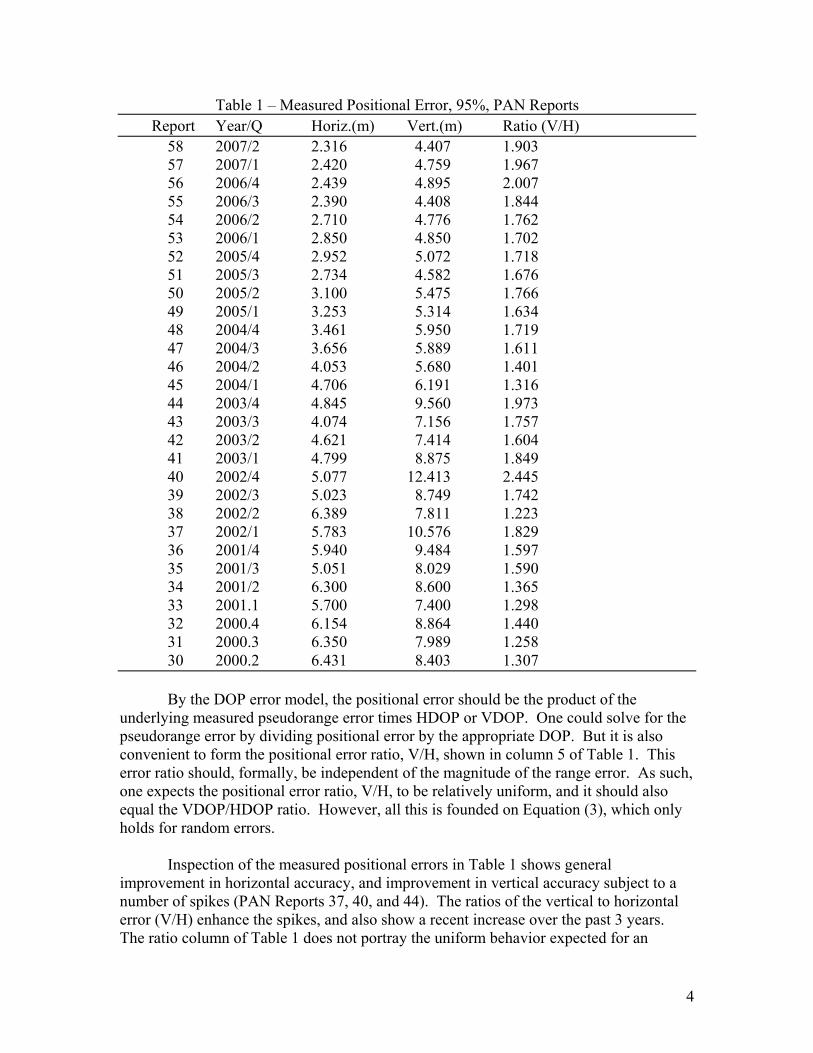
Table 1 – Measured Positional Error, 95%, PAN Reports Report Year/Q Horiz.(m) Vert.(m) Ratio (V/H) 58 2007/2 2.316 4.407 1.903 57 2007/1 2.420 4.759 1.967 56 2006/4 2.439 4.895 2.007 55 2006/3 2.390 4.408 1.844 54 2006/2 2.710 4.776 1.762 53 2006/1 2.850 4.850 1.702 52 2005/4 2.952 5.072 1.718 51 2005/3 2.734 4.582 1.676 50 2005/2 3.100 5.475 1.766 49 2005/1 3.253 5.314 1.634 48 2004/4 3.461 5.950 1.719 47 2004/3 3.656 5.889 1.611 46 2004/2 4.053 5.680 1.401 45 2004/1 4.706 6.191 1.316 44 2003/4 4.845 9.560 1.973 43 2003/3 4.074 7.156 1.757 42 2003/2 4.621 7.414 1.604 41 2003/1 4.799 8.875 1.849 40 2002/4 5.077 12.413 2.445 39 2002/3 5.023 8.749 1.742 38 2002/2 6.389 7.811 1.223 37 2002/1 5.783 10.576 1.829 36 2001/4 5.940 9.484 1.597 35 2001/3 5.051 8.029 1.590 34 2001/2 6.300 8.600 1.365 33 2001.1 5.700 7.400 1.298 32 2000.4 6.154 8.864 1.440 31 2000.3 6.350 7.989 1.258 30 2000.2 6.431 8.403 1.307 By the DOP error model, the positional error should be the product of the underlying measured pseudorange error times HDOP or VDOP. One could solve for the pseudorange error by dividing positional error by the appropriate DOP. But it is also convenient to form the positional error ratio, V/H, shown in column 5 of Table 1. This error ratio should, formally, be independent of the magnitude of the range error. As such, one expects the positional error ratio, V/H, to be relatively uniform, and it should also equal the VDOP/HDOP ratio. However, all this is founded on Equation (3), which only holds for random errors. Inspection of the measured positional errors in Table 1 shows general improvement in horizontal accuracy, and improvement in vertical accuracy subject to a number of spikes (PAN Reports 37, 40, and 44). The ratios of the vertical to horizontal error (V/H) enhance the spikes, and also show a recent increase over the past 3 years. The ratio column of Table 1 does not portray the uniform behavior expected for an

5

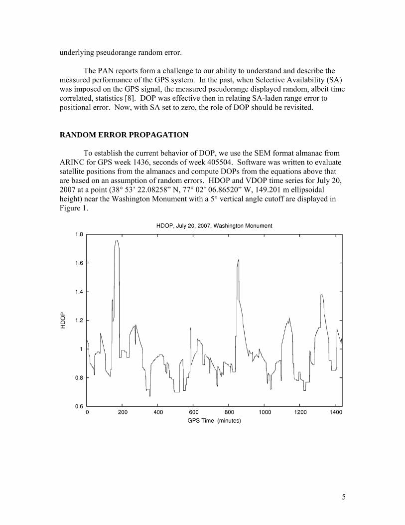
underlying pseudorange random error. The PAN reports form a challenge to our ability to understand and describe the measured performance of the GPS system. In the past, when Selective Availability (SA) was imposed on the GPS signal, the measured pseudorange displayed random, albeit time correlated, statistics [8]. DOP was effective then in relating SA-laden range error to positional error. Now, with SA set to zero, the role of DOP should be revisited. RANDOM ERROR PROPAGATION To establish the current behavior of DOP, we use the SEM format almanac from ARINC for GPS week 1436, seconds of week 405504. Software was written to evaluate satellite positions from the almanacs and compute DOPs from the equations above that are based on an assumption of random errors. HDOP and VDOP time series for July 20, 2007 at a point (38° 53’ 22.08258” N, 77° 02’ 06.86520” W, 149.201 m ellipsoidal height) near the Washington Monument with a 5° vertical angle cutoff are displayed in Figure 1.

6

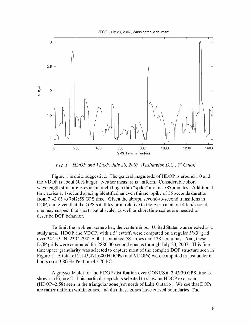
Fig. 1 – HDOP and VDOP, July 20, 2007, Washington D.C., 5° Cutoff Figure 1 is quite suggestive. The general magnitude of HDOP is around 1.0 and the VDOP is about 50% larger. Neither measure is uniform. Considerable short wavelength structure is evident, including a thin “spike” around 585 minutes. Additional time series at 1-second spacing identified an even thinner spike of 55 seconds duration from 7:42:03 to 7:42:58 GPS time. Given the abrupt, second-to-second transitions in DOP, and given that the GPS satellites orbit relative to the Earth at about 4 km/second, one may suspect that short spatial scales as well as short time scales are needed to describe DOP behavior. To limit the problem somewhat, the conterminous United States was selected as a study area. HDOP and VDOP, with a 5° cutoff, were computed on a regular 3’x3’ grid over 24°-53° N, 230°-294° E, that contained 581 rows and 1281 columns. And, these DOP grids were computed for 2880 30-second epochs through July 20, 2007. This fine time/space granularity was selected to capture most of the complex DOP structure seen in Figure 1. A total of 2,143,471,680 HDOPs (and VDOPs) were computed in just under 6 hours on a 3.8GHz Pentium 4-670 PC. A grayscale plot for the HDOP distribution over CONUS at 2:42:30 GPS time is shown in Figure 2. This particular epoch is selected to show an HDOP excursion (HDOP=2.58) seen in the triangular zone just north of Lake Ontario . We see that DOPs are rather uniform within zones, and that these zones have curved boundaries. The

7

boundaries are sharply delineated and move geographically in time, which explains the jumps seen in high-rate DOP time series (e.g. Figure 1). Inspection of sky coverage plots confirms that the curved boundaries are the geographic locations where particular GPS satellites rise or set. Thus, the broad, curved boundaries seen in Figure 2 are the footprints of the various GPS satellites. When Figure 2 is rendered with a linear rainbow color scale, one more easily notices that some of the zones gradually vary in hue. This shows some variation of DOP as the spatial mappings of the local elevation angles change for a given set of GPS satellites in a region.

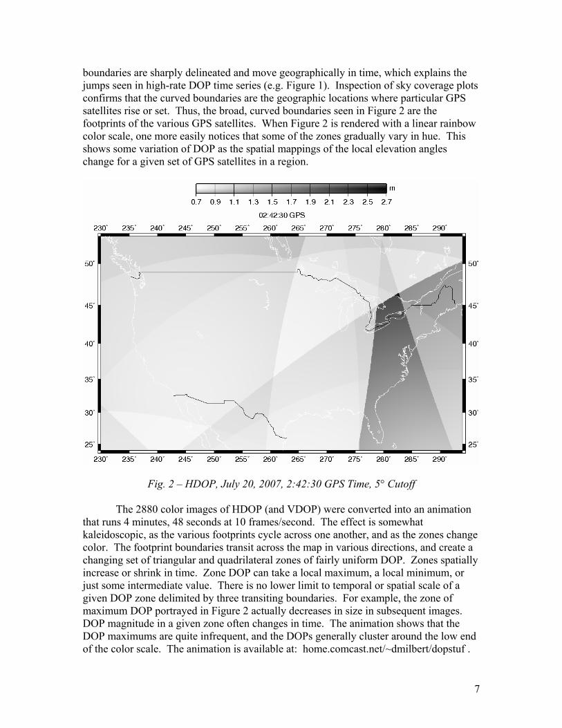
Fig. 2 – HDOP, July 20, 2007, 2:42:30 GPS Time, 5° Cutoff The 2880 color images of HDOP (and VDOP) were converted into an animation that runs 4 minutes, 48 seconds at 10 frames/second. The effect is somewhat kaleidoscopic, as the various footprints cycle across one another, and as the zones change color. The footprint boundaries transit across the map in various directions, and create a changing set of triangular and quadrilateral zones of fairly uniform DOP. Zones spatially increase or shrink in time. Zone DOP can take a local maximum, a local minimum, or just some intermediate value. There is no lower limit to temporal or spatial scale of a given DOP zone delimited by three transiting boundaries. For example, the zone of maximum DOP portrayed in Figure 2 actually decreases in size in subsequent images. DOP magnitude in a given zone often changes in time. The animation shows that the DOP maximums are quite infrequent, and the DOPs generally cluster around the low end of the color scale. The animation is available at: home.comcast.net/~dmilbert/dopstuf .

8

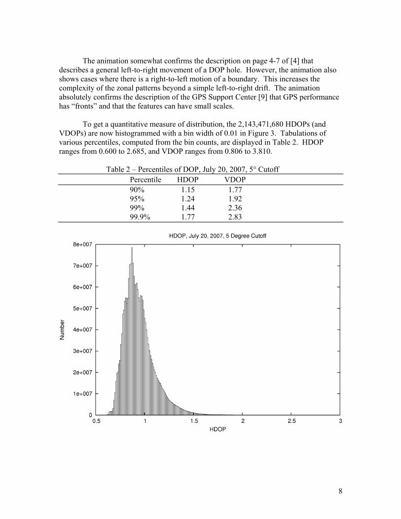
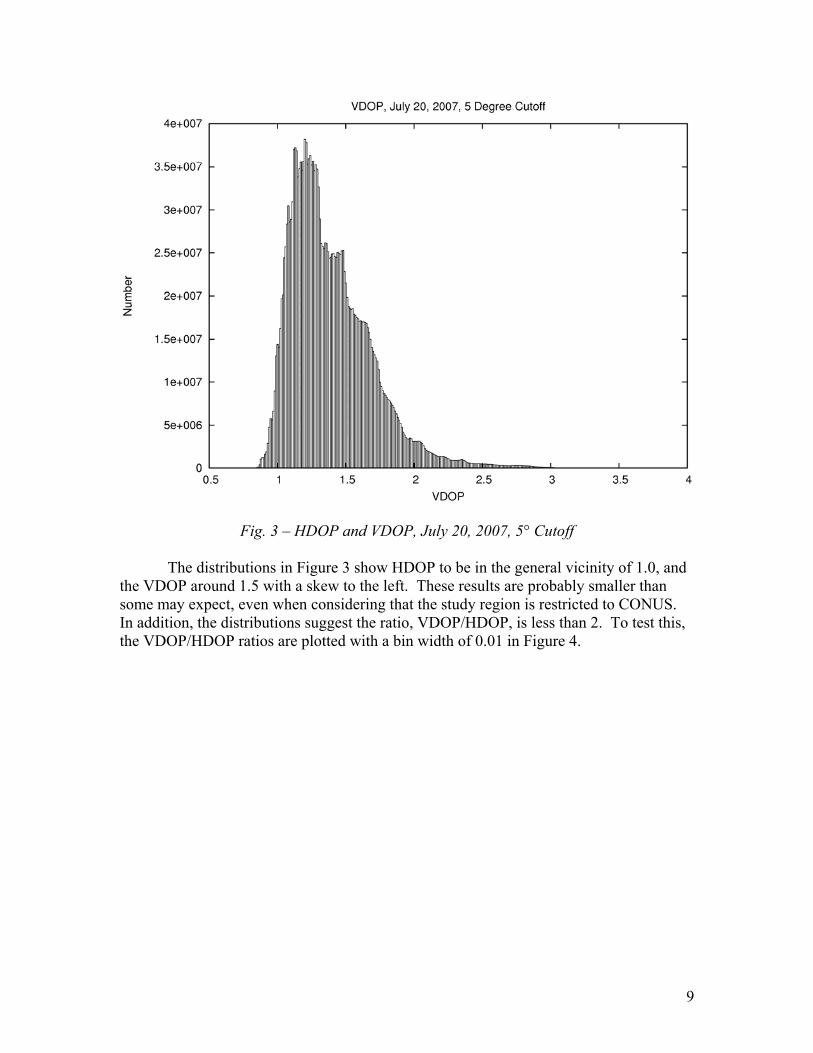
The animation somewhat confirms the description on page 4-7 of [4] that describes a general left-to-right movement of a DOP hole. However, the animation also shows cases where there is a right-to-left motion of a boundary. This increases the complexity of the zonal patterns beyond a simple left-to-right drift. The animation absolutely confirms the description of the GPS Support Center [9] that GPS performance has “fronts” and that the features can have small scales. To get a quantitative measure of distribution, the 2,143,471,680 HDOPs (and VDOPs) are now histogrammed with a bin width of 0.01 in Figure 3. Tabulations of various percentiles, computed from the bin counts, are displayed in Table 2. HDOP ranges from 0.600 to 2.685, and VDOP ranges from 0.806 to 3.810. Table 2 – Percentiles of DOP, July 20, 2007, 5° Cutoff Percentile HDOP VDOP

90% 1.15 1.77 95% 1.24 1.92

99% 1.44 2.36 99.9% 1.77 2.83

9

Fig. 3 – HDOP and VDOP, July 20, 2007, 5° Cutoff The distributions in Figure 3 show HDOP to be in the general vicinity of 1.0, and the VDOP around 1.5 with a skew to the left. These results are probably smaller than some may expect, even when considering that the study region is restricted to CONUS. In addition, the distributions suggest the ratio, VDOP/HDOP, is less than 2. To test this, the VDOP/HDOP ratios are plotted with a bin width of 0.01 in Figure 4.

10

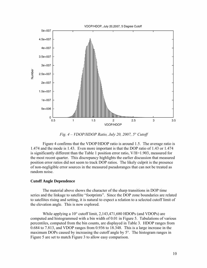
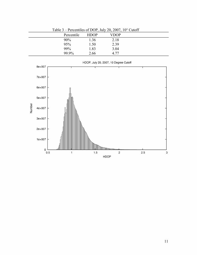
Fig. 4 – VDOP/HDOP Ratio, July 20, 2007, 5° Cutoff Figure 4 confirms that the VDOP/HDOP ratio is around 1.5. The average ratio is 1.474 and the mode is 1.43. Even more important is that the DOP ratio of 1.43 or 1.474 is significantly different than the Table 1 position error ratio, V/H=1.903, measured for the most recent quarter. This discrepancy highlights the earlier discussion that measured position error ratios did not seem to track DOP ratios. The likely culprit is the presence of non-negligible error sources in the measured pseudoranges that can not be treated as random noise. Cutoff Angle Dependence The material above shows the character of the sharp transitions in DOP time series and the linkage to satellite “footprints”. Since the DOP zone boundaries are related to satellites rising and setting, it is natural to expect a relation to a selected cutoff limit of the elevation angle. This is now explored. While applying a 10° cutoff limit, 2,143,471,680 HDOPs (and VDOPs) are computed and histogrammed with a bin width of 0.01 in Figure 5. Tabulations of various percentiles, computed from the bin counts, are displayed in Table 3. HDOP ranges from 0.684 to 7.813, and VDOP ranges from 0.936 to 18.348. This is a large increase in the maximum DOPs caused by increasing the cutoff angle by 5°. The histogram ranges in Figure 5 are set to match Figure 3 to allow easy comparison.

11

Table 3 – Percentiles of DOP, July 20, 2007, 10° Cutoff Percentile HDOP VDOP

90% 1.36 2.18 95% 1.50 2.39

99% 1.83 3.04 99.9% 2.66 4.77

12

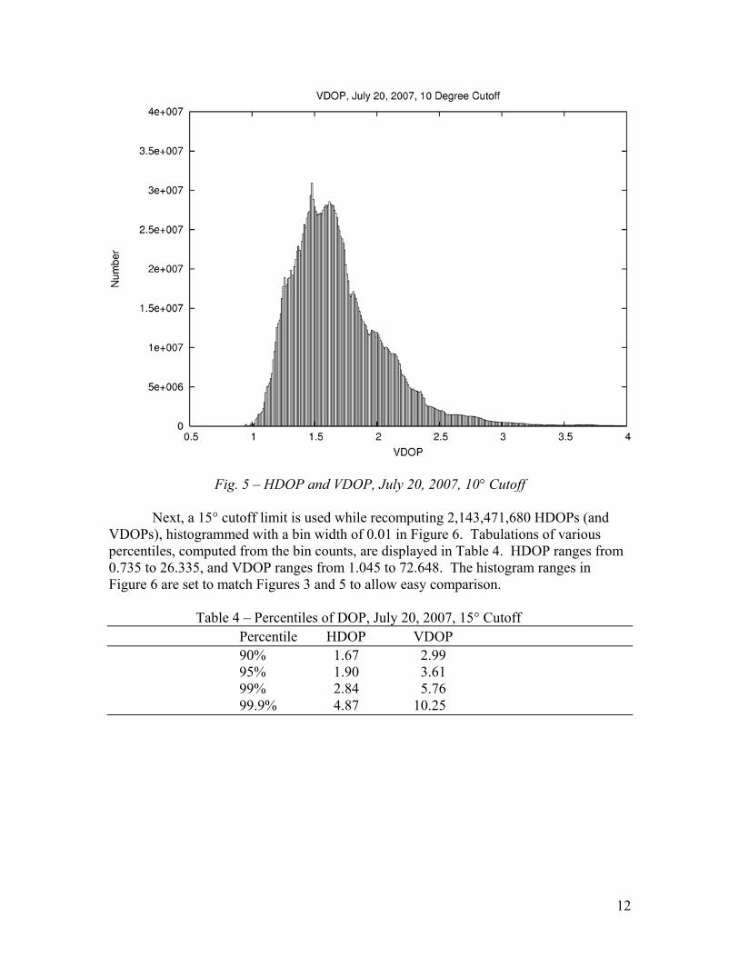
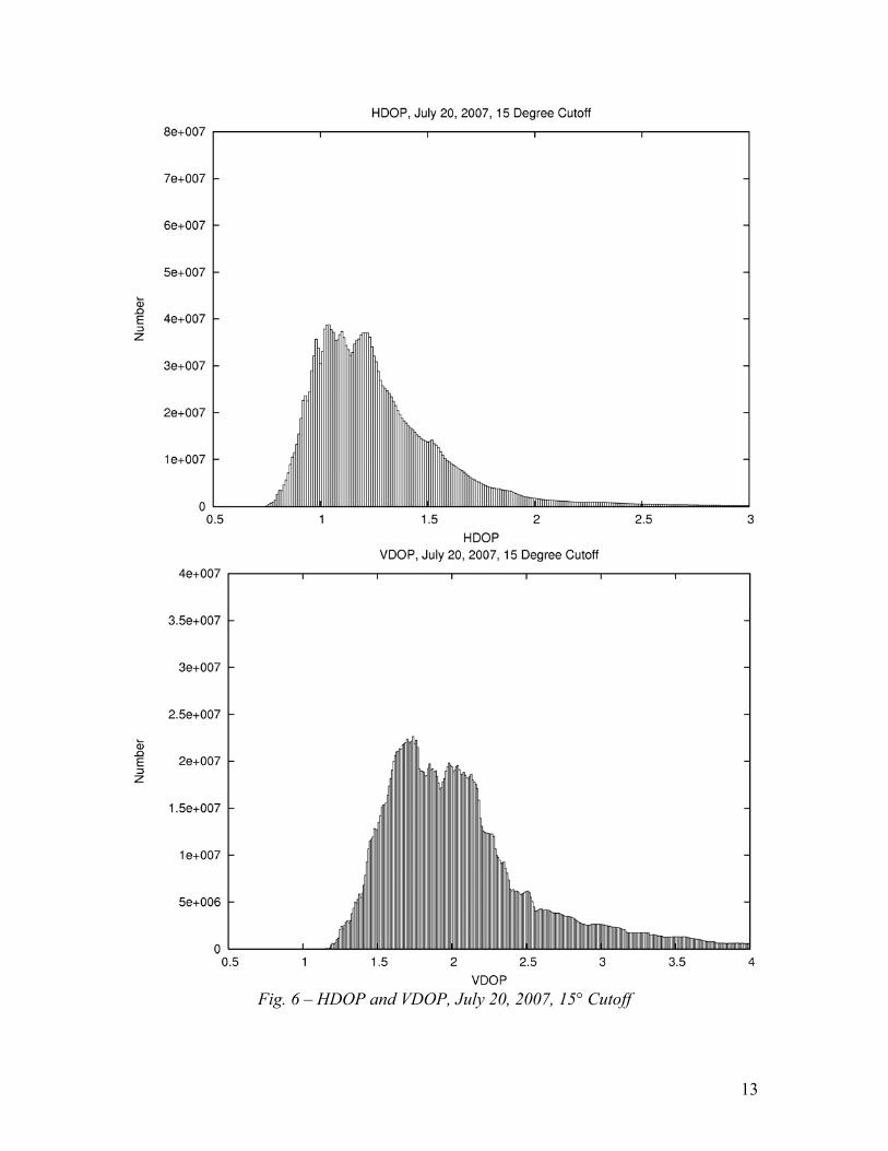
Fig. 5 – HDOP and VDOP, July 20, 2007, 10° Cutoff Next, a 15° cutoff limit is used while recomputing 2,143,471,680 HDOPs (and VDOPs), histogrammed with a bin width of 0.01 in Figure 6. Tabulations of various percentiles, computed from the bin counts, are displayed in Table 4. HDOP ranges from 0.735 to 26.335, and VDOP ranges from 1.045 to 72.648. The histogram ranges in Figure 6 are set to match Figures 3 and 5 to allow easy comparison. Table 4 – Percentiles of DOP, July 20, 2007, 15° Cutoff Percentile HDOP VDOP

90% 1.67 2.99 95% 1.90 3.61

99% 2.84 5.76 99.9% 4.87 10.25

13

Fig. 6 – HDOP and VDOP, July 20, 2007, 15° Cutoff

14

Inspection of the Figures 3, 5, 6 and Tables 2, 3, 4 shows that DOPs are markedly sensitive to cutoff angles. The histogram tails increase, and the maximum DOPs dramatically increase. The 95% HDOP increases by about 50% when the cutoff angle increases from 5° to 15°. The solutions weaken somewhat, and the poorer solutions get much worse. The effect is somewhat greater for VDOP. Implications are profound. One normally considers DOP as a property of the satellite constellation that has a space-time mapping. DOP is seen to strongly depend upon horizon visibility. This is a completely local property that is highly variable throughout the country. In short, DOP depends on the antenna site as well as the constellation. In a single experiment described in the Appendix, cutoff angle is seen to be more important than the constellation population. SYSTEMATIC ERROR PROPAGATION It is known that certain error sources in GPS are systematic and, as such, display different behaviors from random error. [10] describes the cancellation of ionospheric delay in position solutions and offers an analysis. This point is reiterated in [11], who also state that residual ionospheric error should not be considered random. Section 7.3.2 of [5] recognizes the systematic error correlation between satellites invalidates the assumption of random error propagation of DOPs. And, as described earlier, [6] points out the failure of VDOP to characterize tropospheric error. New metrics for systematic positional error are needed.

Consider a systematic bias, b, in measured pseudorange, R. One may propagate the bias, b, through the least squares adjustment (1) by setting y = b. Vector x then contains the differential change (error) in coordinates (δx, δy, δz, δt) induced by the bias. The coordinate error can then be expressed in the local geodetic horizon system by xh = G x (7) And, the positional systematic error is defined as Horizontal Error (δN2 + δE2) ½ (8) Vertical Error |δU| As with DOP, the system of equations (1), (7), and (8) is linear for any measurement bias scale factor, k that applies to all satellite pseudoranges in an epoch. Thus, if one halves the bias that applies to all pseudoranges (e.g. ky) then one will halve the associated coordinate error, kx and kxh. Analogous to DOP, we take bias as units of meters with a base error b=1, and designate the resulting measures (8) as Horizontal Error Scale Factor (HESF), and Vertical Error Scale Factor (VESF). This adds a capability of developing error budgets for systematic effects that parallels DOP. Systematic errors in GPS position solutions have a distinctly different behavior

15

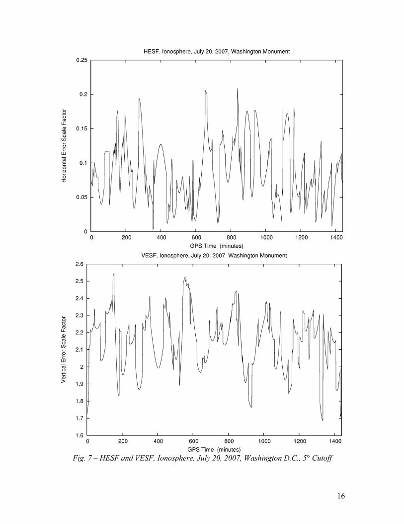
than random errors. This is illustrated by a trivial example that is presented to emphasize this point. If one repeats any of the tests above with a constant value of b, one will find that, aside from computer roundoff error, no systematic error propagates into the position. The coordinates are recovered perfectly, and the bias, b, is absorbed into the receiver time bias parameter, dt. This is no surprise, since the model (2) is constructed to solve for a constant bias. Of interest is that the coordinate recovery is uniformly perfect irrespective of the values of DOP. See [10] for an algebraic analysis of systematic error transfer into dt. Of the errors that contaminate pseudoranges, many of them seem systematic when considered for one or two epochs, but will soon yield random statistics when considered over spans of time or over the entire constellation. Multipath, for example, plagues low elevation angle measurements. But multipath will not be in phase for two satellites at the same elevation angle. Thus, the “all satellites in view” system (1) will not tend to absorb multipath error into the dt parameter. Ionosphere and troposphere, on the other hand, cause systematic error in pseudoranges that are common to all satellites. These systematic errors are greater for lower elevation satellites than for higher elevation satellites. So, unlike the trivial example above, this error can not be perfectly absorbed into dt. However, the systematics never vanish, even for satellites at zenith. One may expect some resulting positional error that does not behave randomly. The systematic effect of ionosphere and troposphere differ through their mapping functions. These are functions of elevation angle, E, and are scale factors to the systematic effect at zenith (E=90°). Because of the different altitudes of these atmospheric layers, the mapping functions take different forms. For this reason, systematic error scale factors (ESFs) for ionosphere and troposphere must be considered separately. Ionosphere Error Scale Factor Following Figure 20-6 of the IS-GPS-200D [12], the ionospheric mapping function, F, is F = 1.0 + 16.0 (0.53 - E)3 (E in semicircles) (9) and where semicircles are angular units of 180 degrees and of π radians. Since the base error is considered b=1 for ESFs, y is simply populated with the various values of F appropriate to the elevation angles, E, of the various satellites visible at a given epoch. HESF and VESF ionosphere time series for July 20, 2007 at a point (38° 53’ 22.08258” N, 77° 02’ 06.86520” W, 149.201 m ellipsoidal height) near the Washington Monument with a 5° vertical angle cutoff are displayed in Figure 7. The figure portrays how systematic ionosphere error will be magnified into positional error, just as DOPs portray how random pseudorange error is magnified into positional error.

16

Fig. 7 – HESF and VESF, Ionosphere, July 20, 2007, Washington D.C., 5° Cutoff

17

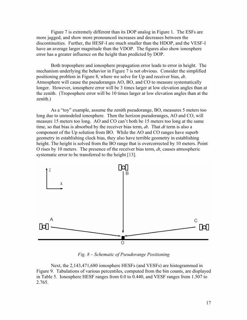
Figure 7 is extremely different than its DOP analog in Figure 1. The ESFs are more jagged, and show more pronounced increases and decreases between the discontinuities. Further, the HESF-I are much smaller than the HDOP, and the VESF-I have an average larger magnitude than the VDOP. The figures also show ionosphere error has a greater influence on the height than predicted by DOP. Both troposphere and ionosphere propagation error leads to error in height. The mechanism underlying the behavior in Figure 7 is not obvious. Consider the simplified positioning problem in Figure 8, where we solve for Up and receiver bias, dt. Atmosphere will cause the pseudoranges AO, BO, and CO to measure systematically longer. However, ionosphere error will be 3 times larger at low elevation angles than at the zenith. (Troposphere error will be 10 times larger at low elevation angles than at the zenith.) As a “toy” example, assume the zenith pseudorange, BO, measures 5 meters too long due to unmodeled ionosphere. Then the horizon pseudoranges, AO and CO, will measure 15 meters too long. AO and CO can’t both be 15 meters too long at the same time, so that bias is absorbed by the receiver bias term, dt. That dt term is also a component of the Up solution from BO. While the AO and CO ranges have superb geometry in establishing clock bias, they also have terrible geometry in establishing height. The height is solved from the BO range that is overcorrected by 10 meters. Point O rises by 10 meters. The presence of the receiver bias term, dt, causes atmospheric systematic error to be transferred to the height [13].

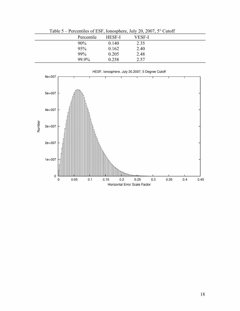
Fig. 8 – Schematic of Pseudorange Positioning Next, the 2,143,471,680 ionosphere HESFs (and VESFs) are histogrammed in Figure 9. Tabulations of various percentiles, computed from the bin counts, are displayed in Table 5. Ionosphere HESF ranges from 0.0 to 0.440, and VESF ranges from 1.507 to 2.765.

18

Table 5 – Percentiles of ESF, Ionosphere, July 20, 2007, 5° Cutoff Percentile HESF-I VESF-I

90% 0.140 2.35 95% 0.162 2.40

99% 0.205 2.48 99.9% 0.258 2.57

19

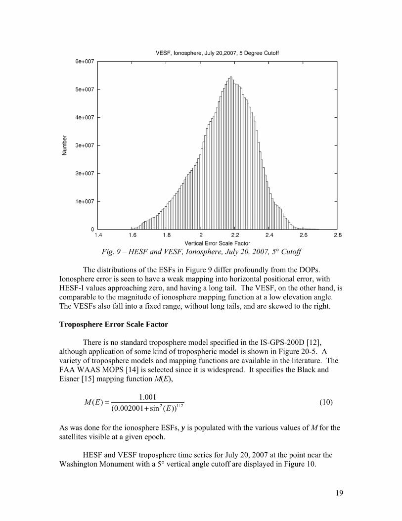
Fig. 9 – HESF and VESF, Ionosphere, July 20, 2007, 5° Cutoff

The distributions of the ESFs in Figure 9 differ profoundly from the DOPs. Ionosphere error is seen to have a weak mapping into horizontal positional error, with HESF-I values approaching zero, and having a long tail. The VESF, on the other hand, is comparable to the magnitude of ionosphere mapping function at a low elevation angle. The VESFs also fall into a fixed range, without long tails, and are skewed to the right. Troposphere Error Scale Factor There is no standard troposphere model specified in the IS-GPS-200D [12], although application of some kind of tropospheric model is shown in Figure 20-5. A variety of troposphere models and mapping functions are available in the literature. The FAA WAAS MOPS [14] is selected since it is widespread. It specifies the Black and Eisner [15] mapping function M(E),

2/12 ))(sin002001.0(001.1)(

EEM

+= (10)

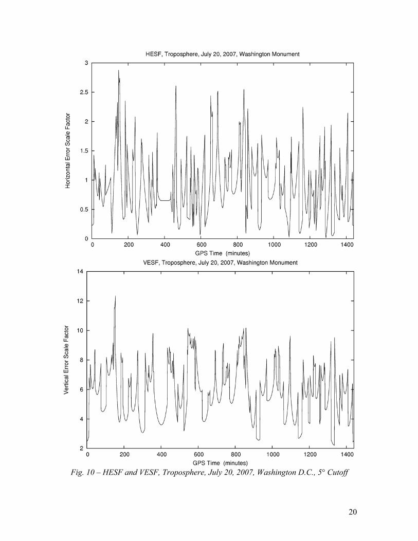
As was done for the ionosphere ESFs, y is populated with the various values of M for the satellites visible at a given epoch. HESF and VESF troposphere time series for July 20, 2007 at the point near the Washington Monument with a 5° vertical angle cutoff are displayed in Figure 10.

20

Fig. 10 – HESF and VESF, Troposphere, July 20, 2007, Washington D.C., 5° Cutoff

21

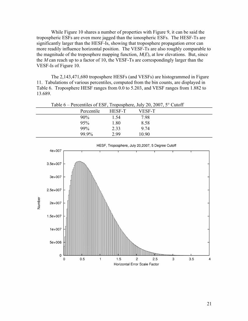
While Figure 10 shares a number of properties with Figure 9, it can be said the tropospheric ESFs are even more jagged than the ionospheric ESFs. The HESF-Ts are significantly larger than the HESF-Is, showing that troposphere propagation error can more readily influence horizontal position. The VESF-Ts are also roughly comparable to the magnitude of the troposphere mapping function, M(E), at low elevations. But, since the M can reach up to a factor of 10, the VESF-Ts are correspondingly larger than the VESF-Is of Figure 10. The 2,143,471,680 troposphere HESFs (and VESFs) are histogrammed in Figure 11. Tabulations of various percentiles, computed from the bin counts, are displayed in Table 6. Troposphere HESF ranges from 0.0 to 5.203, and VESF ranges from 1.882 to 13.689. Table 6 – Percentiles of ESF, Troposphere, July 20, 2007, 5° Cutoff Percentile HESF-T VESF-T

90% 1.54 7.98 95% 1.80 8.58

99% 2.33 9.74 99.9% 2.99 10.90

22

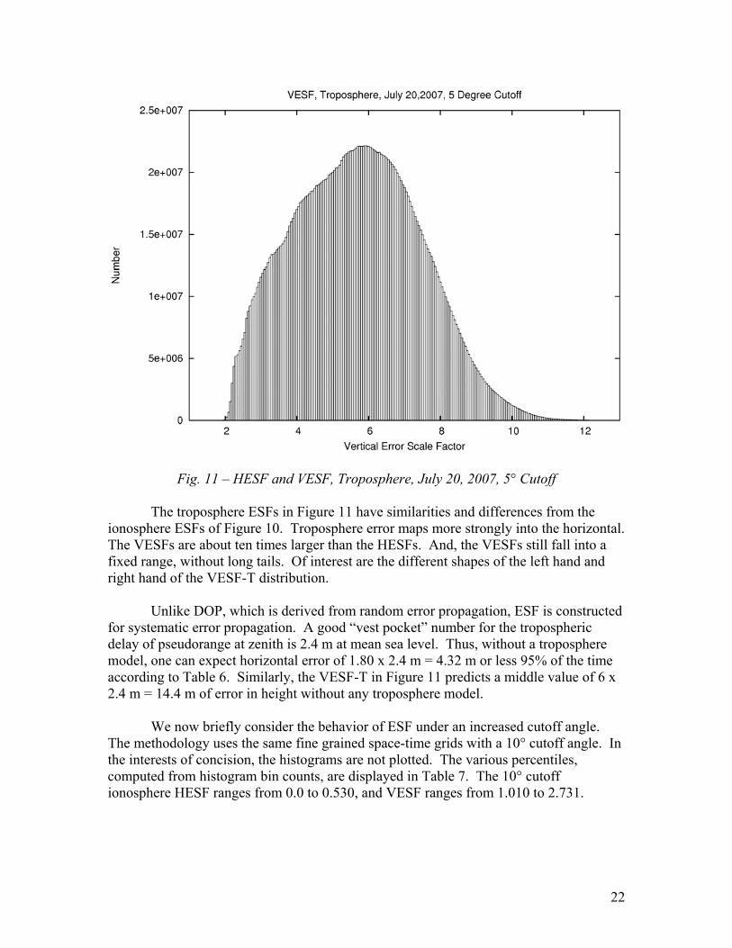
Fig. 11 – HESF and VESF, Troposphere, July 20, 2007, 5° Cutoff The troposphere ESFs in Figure 11 have similarities and differences from the ionosphere ESFs of Figure 10. Troposphere error maps more strongly into the horizontal. The VESFs are about ten times larger than the HESFs. And, the VESFs still fall into a fixed range, without long tails. Of interest are the different shapes of the left hand and right hand of the VESF-T distribution. Unlike DOP, which is derived from random error propagation, ESF is constructed for systematic error propagation. A good “vest pocket” number for the tropospheric delay of pseudorange at zenith is 2.4 m at mean sea level. Thus, without a troposphere model, one can expect horizontal error of 1.80 x 2.4 m = 4.32 m or less 95% of the time according to Table 6. Similarly, the VESF-T in Figure 11 predicts a middle value of 6 x 2.4 m = 14.4 m of error in height without any troposphere model. We now briefly consider the behavior of ESF under an increased cutoff angle. The methodology uses the same fine grained space-time grids with a 10° cutoff angle. In the interests of concision, the histograms are not plotted. The various percentiles, computed from histogram bin counts, are displayed in Table 7. The 10° cutoff ionosphere HESF ranges from 0.0 to 0.530, and VESF ranges from 1.010 to 2.731.

23

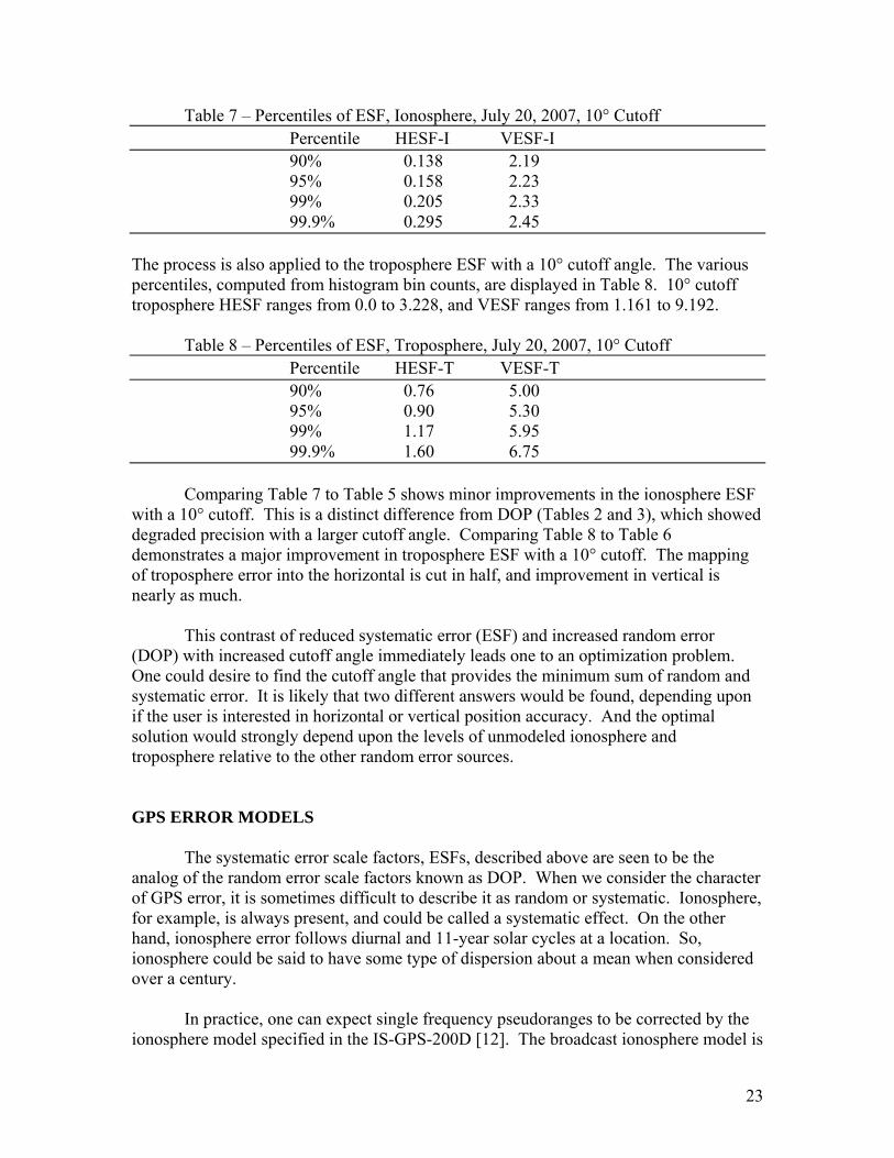
Table 7 – Percentiles of ESF, Ionosphere, July 20, 2007, 10° Cutoff Percentile HESF-I VESF-I

90% 0.138 2.19 95% 0.158 2.23

99% 0.205 2.33 99.9% 0.295 2.45 The process is also applied to the troposphere ESF with a 10° cutoff angle. The various percentiles, computed from histogram bin counts, are displayed in Table 8. 10° cutoff troposphere HESF ranges from 0.0 to 3.228, and VESF ranges from 1.161 to 9.192. Table 8 – Percentiles of ESF, Troposphere, July 20, 2007, 10° Cutoff Percentile HESF-T VESF-T

90% 0.76 5.00 95% 0.90 5.30

99% 1.17 5.95 99.9% 1.60 6.75 Comparing Table 7 to Table 5 shows minor improvements in the ionosphere ESF with a 10° cutoff. This is a distinct difference from DOP (Tables 2 and 3), which showed degraded precision with a larger cutoff angle. Comparing Table 8 to Table 6 demonstrates a major improvement in troposphere ESF with a 10° cutoff. The mapping of troposphere error into the horizontal is cut in half, and improvement in vertical is nearly as much. This contrast of reduced systematic error (ESF) and increased random error (DOP) with increased cutoff angle immediately leads one to an optimization problem. One could desire to find the cutoff angle that provides the minimum sum of random and systematic error. It is likely that two different answers would be found, depending upon if the user is interested in horizontal or vertical position accuracy. And the optimal solution would strongly depend upon the levels of unmodeled ionosphere and troposphere relative to the other random error sources. GPS ERROR MODELS The systematic error scale factors, ESFs, described above are seen to be the analog of the random error scale factors known as DOP. When we consider the character of GPS error, it is sometimes difficult to describe it as random or systematic. Ionosphere, for example, is always present, and could be called a systematic effect. On the other hand, ionosphere error follows diurnal and 11-year solar cycles at a location. So, ionosphere could be said to have some type of dispersion about a mean when considered over a century. In practice, one can expect single frequency pseudoranges to be corrected by the ionosphere model specified in the IS-GPS-200D [12]. The broadcast ionosphere model is

24

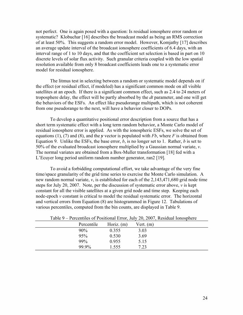
not perfect. One is again posed with a question: Is residual ionosphere error random or systematic? Klobuchar [16] describes the broadcast model as being an RMS correction of at least 50%. This suggests a random error model. However, Komjathy [17] describes an average update interval of the broadcast ionosphere coefficients of 6.4 days, with an interval range of 1 to 10 days, and that the coefficient set selection is based in part on 10 discrete levels of solar flux activity. Such granular criteria coupled with the low spatial resolution available from only 8 broadcast coefficients leads one to a systematic error model for residual ionosphere. The litmus test in selecting between a random or systematic model depends on if the effect (or residual effect, if modeled) has a significant common mode on all visible satellites at an epoch. If there is a significant common effect, such as 2.4 to 24 meters of troposphere delay, the effect will be partly absorbed by the dt parameter, and one will get the behaviors of the ESFs. An effect like pseudorange multipath, which is not coherent from one pseudorange to the next, will have a behavior closer to DOPs. To develop a quantitative positional error description from a source that has a short term systematic effect with a long term random behavior, a Monte Carlo model of residual ionosphere error is applied. As with the ionospheric ESFs, we solve the set of equations (1), (7) and (8), and the y vector is populated with Fb, where F is obtained from Equation 9. Unlike the ESFs, the base error, b, is no longer set to 1. Rather, b is set to 50% of the evaluated broadcast ionosphere multiplied by a Gaussian normal variate, v. The normal variates are obtained from a Box-Muller transformation [18] fed with a L’Ecuyer long period uniform random number generator, ran2 [19]. To avoid a forbidding computational effort, we take advantage of the very fine time/space granularity of the grid time series to exercise the Monte Carlo simulation. A new random normal variate, v, is established for each of the 2,143,471,680 grid node time steps for July 20, 2007. Note, per the discussion of systematic error above, v is kept constant for all the visible satellites at a given grid node and time step. Keeping each node-epoch v constant is critical to model the residual systematic error. The horizontal and vertical errors from Equation (8) are histogrammed in Figure 12. Tabulations of various percentiles, computed from the bin counts, are displayed in Table 9. Table 9 – Percentiles of Positional Error, July 20, 2007, Residual Ionosphere Percentile Horiz. (m) Vert. (m)

90% 0.355 3.03 95% 0.530 3.69

99% 0.955 5.15 99.9% 1.555 7.23

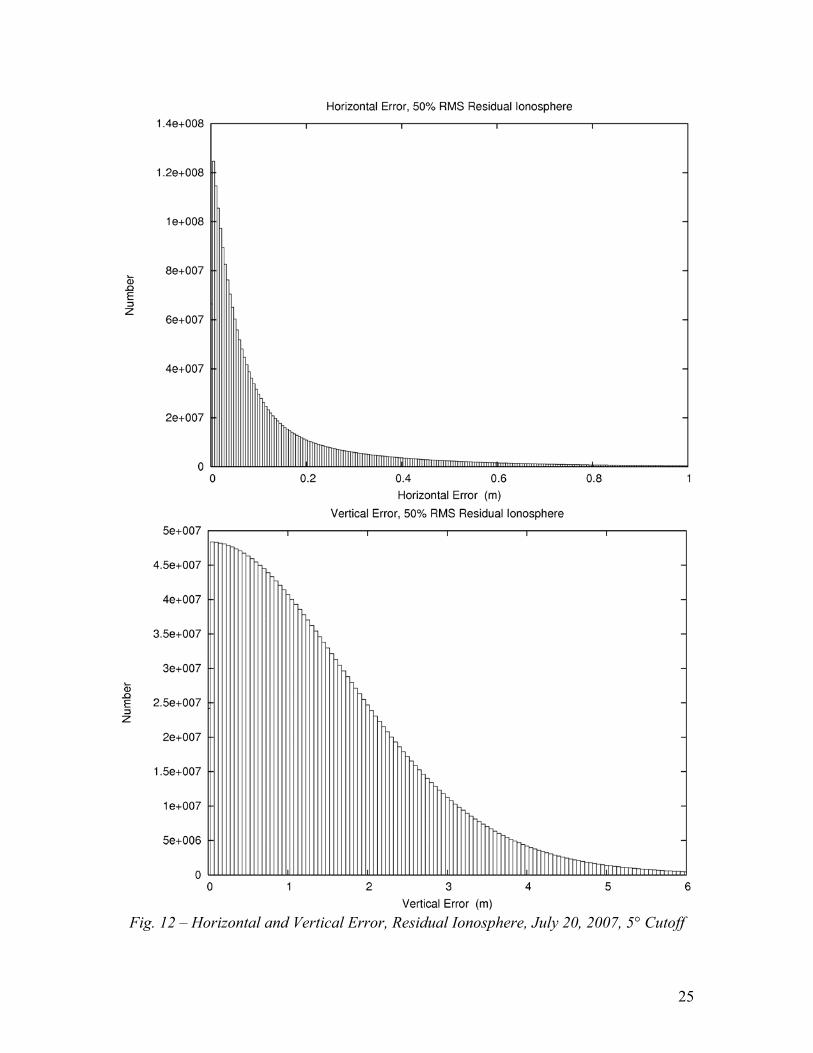
25

Fig. 12 – Horizontal and Vertical Error, Residual Ionosphere, July 20, 2007, 5° Cutoff

26

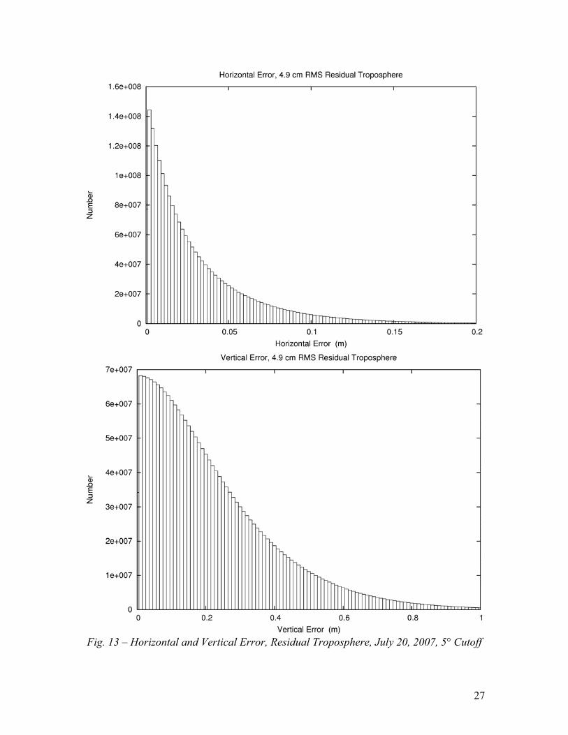
The positional error due to residual ionosphere distributions in Figure 12 is based on the broadcast ionosphere of July 20, 2007, and would certainly vary at other times of the solar cycle. In addition, the 50% RMS value, itself, coupled with the ionosphere coefficient selection process, deserves additional exploration. The discussion describes possible refinements. As mentioned earlier, the IS-GPS-200D [12] does not specify a troposphere model. We consider the FAA WAAS [14] troposphere model instead. An excellent analysis by Collins and Langley [6] shows residual troposphere error of 4.9 cm RMS subject to a remaining 2 cm systematic bias. That 2 cm residual bias can be directly scaled by the HESF-T and VSEF-T values in Figure 11 and Table 8 to get a portion of the troposphere residual error. Alternatively, one could choose a new, modified version of the model, UNB3m [20]. The UNB3m model removes most of the residual bias, and maintains the small RMS residual troposphere error. To get the positional error due to 4.9 cm RMS of residual troposphere error, the Monte Carlo method described above is applied with the Black and Eisner tropospheric mapping function [15] of Equation (10) and b=0.049. While UNB3m does specify the Niell mapping functions [21], the WAAS protocol is retained since little difference was noted in Collins and Langley [6]. Since the troposphere model is expected to overpredict or underpredict for all visible satellites at an epoch and location, the Gaussian normal variate, v, is kept constant for all the visible satellites at each given grid node and time step, as was done for Figure 12 and Table 9.

The horizontal and vertical errors from Equation (8) are histogrammed in Figure 13. Tabulations of various percentiles, computed from the bin counts, are displayed in Table 10. Table 10 – Percentiles of Positional Error, Residual Troposphere Percentile Horiz. (m) Vert. (m)

90% 0.08 0.48 95% 0.10 0.60

99% 0.16 0.84 99.9% 0.26 1.17

27

Fig. 13 – Horizontal and Vertical Error, Residual Troposphere, July 20, 2007, 5° Cutoff

28

The horizontal residual troposphere error is seen to be negligible. It is notable that the horizontal 95% percentile is about double the RMS residual troposphere model error. The residual troposphere error, on the other hand, has a much larger effect on vertical position error. The vertical 95% percentile is six times larger than the horizontal, which is slightly less than the approximation reported by Collins and Langley [6]. The magnitude of the troposphere mapping function at low elevation angles in conjunction with the action of the dt bias parameter lead to a bigger vertical error effect than predicted from simple VDOP scaling of a 4.9 cm RMS residual troposphere error. We close this section by providing a first attempt of a calibrated error model derived from the PAN measurements that accommodates both random error and systematic error behaviors. To begin, consider the simple random error model (as found in Appendix B of the PPS-PS [1]) Mh = r Dh (11) Mv = r Dv where r denotes an unknown calibration coefficient for random error, and where Dh is HDOP 95% percentile at 5° cutoff (1.24 by Table 2) Dv is VDOP 95% percentile at 5° cutoff (1.92 by Table 2) Mh is measured 95% percentile horizontal error (varies with PAN #, Table 1) Mv is measured 95% percentile vertical error (varies with PAN #, Table 1). One immediately sees by inspection that we have not one, but two estimates of r for each PAN report. And, these estimates are inconsistent. Now, add the ionosphere and troposphere components to produce a hybrid error model Mh

2 = r2 Dh2 + i2 Ih

2 + t2 Th2 (12)

Mv2 = r2 Dv

2 + i2 Iv2 + t2 Tv

2 where i denotes an unknown calibration coefficient for residual ionosphere systematic error, and where Ih is HESF-I 95% percentile at 5° cutoff (0.162 by Table 5) Iv is VESF-I 95% percentile at 5° cutoff (2.40 by Table 5) t is a coefficient for residual troposphere systematic error Th is HESF-T 95% percentile at 5° cutoff Tv is VESF-T 95% percentile at 5° cutoff. Given the inability to solve for 3 coefficients with 2 positional error measures in a quarter, we treat the residual troposphere as resolved, and substitute the 95% values from Table 10:

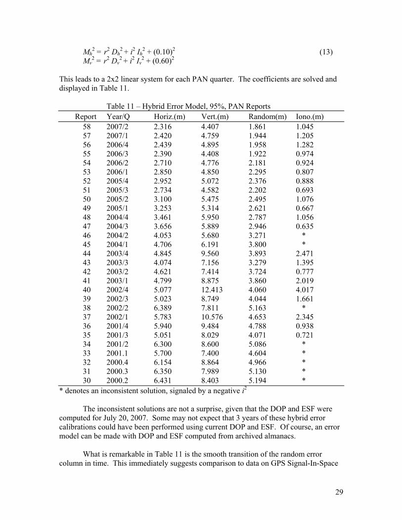
29

Mh2 = r2 Dh

2 + i2 Ih2 + (0.10)2 (13)

Mv2 = r2 Dv

2 + i2 Iv2 + (0.60)2

This leads to a 2x2 linear system for each PAN quarter. The coefficients are solved and displayed in Table 11. Table 11 – Hybrid Error Model, 95%, PAN Reports Report Year/Q Horiz.(m) Vert.(m) Random(m) Iono.(m) 58 2007/2 2.316 4.407 1.861 1.045 57 2007/1 2.420 4.759 1.944 1.205 56 2006/4 2.439 4.895 1.958 1.282 55 2006/3 2.390 4.408 1.922 0.974 54 2006/2 2.710 4.776 2.181 0.924 53 2006/1 2.850 4.850 2.295 0.807 52 2005/4 2.952 5.072 2.376 0.888 51 2005/3 2.734 4.582 2.202 0.693 50 2005/2 3.100 5.475 2.495 1.076 49 2005/1 3.253 5.314 2.621 0.667 48 2004/4 3.461 5.950 2.787 1.056 47 2004/3 3.656 5.889 2.946 0.635 46 2004/2 4.053 5.680 3.271 * 45 2004/1 4.706 6.191 3.800 * 44 2003/4 4.845 9.560 3.893 2.471 43 2003/3 4.074 7.156 3.279 1.395 42 2003/2 4.621 7.414 3.724 0.777 41 2003/1 4.799 8.875 3.860 2.019 40 2002/4 5.077 12.413 4.060 4.017 39 2002/3 5.023 8.749 4.044 1.661 38 2002/2 6.389 7.811 5.163 * 37 2002/1 5.783 10.576 4.653 2.345 36 2001/4 5.940 9.484 4.788 0.938 35 2001/3 5.051 8.029 4.071 0.721 34 2001/2 6.300 8.600 5.086 * 33 2001.1 5.700 7.400 4.604 * 32 2000.4 6.154 8.864 4.966 * 31 2000.3 6.350 7.989 5.130 * 30 2000.2 6.431 8.403 5.194 * * denotes an inconsistent solution, signaled by a negative i2 The inconsistent solutions are not a surprise, given that the DOP and ESF were computed for July 20, 2007. Some may not expect that 3 years of these hybrid error calibrations could have been performed using current DOP and ESF. Of course, an error model can be made with DOP and ESF computed from archived almanacs. What is remarkable in Table 11 is the smooth transition of the random error column in time. This immediately suggests comparison to data on GPS Signal-In-Space

30

(SIS) User Range Error (URE). Figures of SIS URE by the GPS Operations Center [22] portray average values of about 1.05 m for January 1, 2006 and about 0.97 m for July 20, 2007. Table 11 shows larger reduction in random error over the same interval. Ionosphere error is likely to have been only partially calibrated by the error fitting procedure. This also suggests that average SIS URE is another data set which can be brought to bear on the hybrid error model calibration problem. This hybrid error model is just a first attempt at simultaneously reconciling random and systematic effects. It shows some capability to filter ionosphere error from other truly random noise sources. Consider that this preliminary model only used July 20, 2007 DOP and ESF values to fit 29 quarters of data that reached back to 2000. In addition, both DOP and ESF are sensitive to cutoff angle, and it was assumed that a 5° cutoff was suitable for the PAN network. The 95% percentile from the PAN reports was chosen since it was the only comprehensive statistic provided. A 50% percentile, if it had been provided, is a more robust statistic. Despite these factors, the model does relate measured PAN statistics to a consistent set of error budget coefficients. This hybrid error model is partially successful in quantifying both random and systematic error sources. DISCUSSION DOP was first applied to GPS positioning 30 years ago in [2]. Since that time, the GPS system has evolved to where it is capable of SIS URE of about 1 meter [22], and CONUS horizontal positions better than 2.5 meters 95% of the time [7]. The assumption of atmospheric error having a random effect on the single frequency point position problem is now seen to have broken down. We are currently in the solar cycle minimum, and the systematic error from the ionosphere will have an even larger share of the error budget in the coming years. Systematic error propagation needs to be considered. This study can be extended in numerous ways. For example, global error distribution could be measured by means of the International GNSS Service (IGS) [23] tracking network much as the PAN network does. The exact cutoff angles for each of the PAN network stations could be established from analysis of the GPS raw data in the Continuously Operating Reference Stations (CORS) archives of the National Geodetic Survey [24]. In principle, it would be possible to reproduce PAN analysis from the CORS data, as well as supplement it with other stations. Additional data sets can be used to construct more sophisticated error budgets. Mention was made above of the GPS Operations Center daily assessment of SIS URE [22]. Performance of the broadcast ionosphere model could be independently assessed by means of IGS ionosphere TEC grids, ionosphere products from the Center for Orbit Determination in Europe (CODE) [25], or the real-time ionosphere product by NOAA [26]. Similarly, one can independently assess some reference troposphere model, such as UNB3m [20], by means of IGS troposphere grids, UNB online products [27], and the NOAA GPS-Met network [28]. (Note that [27] currently displays images of the performance of UNB3 and UNB3m compared to their new models.)

31

Additional data enables extension of the hybrid error model of Equation (12) by adding more observation equations and error budget components. A least squares adjustment solves this more elaborate system. One might also tailor the error model calibration to the monitor stations, as demonstrated by the comprehensive 95% percentile data found in Table 5-1 of the PAN reports [7]. Here, one constructs multiple instances of Equation (12), but using the DOP and ESF unique to each monitor station. As an alternative approach to quantifying systematic error propagation by Equations (1), (7) and (8), one could study the “DOP-like” quantities that arise from more sophisticated treatments of the pseudorange covariance matrix, Q. For example, Equation (7.68) of [5] describes a covariance matrix that not only deweights low elevation angle satellites, but also introduces correlations reflecting the geometry of the ionosphere mapping function (Eq. 9). It would be interesting to see how such weight-based approaches would compare to ESF in construction of GPS error models. CONCLUSIONS Computation of measured vertical to horizontal positional error ratios from FAA PAN report data shows non-uniform behavior inconsistent with the random error propagation model of DOP. Computation and animation of HDOP and VDOP at a 30 second interval on a regular 3’x3’ grid demonstrate that DOP has broad, curved, and distinct boundaries reflecting satellite footprints. The motion of these boundaries leads to intersections and zones (e.g. DOP “holes”) that can be arbitrarily small in space and time. For CONUS on July 20, 2007 the 95% percentile is 1.24 for HDOP and 1.92 for VDOP. The mean VDOP/HDOP ratio is 1.474, which does not match the most recent measured PAN positional error ratio. DOP is sensitive to cutoff angle. The 95% HDOP increases by about 50% when the cutoff angle increases from 5° to 15°. The effect is somewhat greater for VDOP. DOP is a local property, depending upon the antenna site and horizon visibility. A new measure, Error Scale Factor (ESF), is defined which scales systematic error sources and which is analogous to DOP. Due to the differing elevation angle mapping functions, ESF is further categorized into ionosphere and troposphere forms. ESF has distinctly different behaviors than DOP. The 95% percentiles for ionosphere HESF and VESF are 0.162 and 2.40, respectively. The troposphere ESFs are 1.80 and 8.58. The marked sensitivity of vertical error to systematic pseudorange error is due to the solution of the unknown receiver clock bias parameter in the point positioning problem. Less systematic error will map into positional error if one increases cutoff angle. This behavior is the reverse of DOP, and allows the formulation of an optimization problem. Systematic error is not completely removed by existing atmosphere models. Both residual ionosphere error and residual troposphere error are systematic when inspecting their effects on pseudoranges at a single epoch, and the associated transfer of bias into the

32

receiver clock parameter. A Monte Carlo simulation shows 50% RMS residual ionosphere error for July 20, 2007 maps into 95% percentiles of 0.53 m of horizontal and 3.69 m of vertical error. A related Monte Carlo simulation demonstrates that 4.9 cm RMS residual troposphere error maps into 95% percentiles of 0.10 m of horizontal and 0.60 m of vertical error. A hybrid error model is constructed which relates measured PAN statistics to a consistent set of error budget coefficients. This hybrid error model is partially successful in quantifying both random and systematic error sources. ACKNOWLEDGEMENTS Thanks are extended to ARINC, whose WSEM provided reference values to test correct software operation. Thank you to the contributors to the open source software, Gnuplot. I thank Drs. Wessel and Smith for building the Generic Mapping Tools software which rendered the animation frames. Thank you to the contributors to the open source software VirtualDubMod and the XviD codec (construct and play the animation). Thanks to Dr. Dru Smith and Dr. Chris Hegarty for their early review and helpful suggestions. Thank you to an anonymous reviewer who provided thoughful comments and suggested further consideration of Equation (7.68) in [5]. Thanks are also expressed to the men and women of the GPS Operations Center (2SOPS), whose efforts have lead to the outstanding accuracies depicted in this paper. APPENDIX The focus of this paper has been an exploration of the relationship of DOP to recent, measured GPS performance. However, the temptation to consider alternative, hypothetical constellation configurations is irresistible. In particular, the current (August 2007) constellation has 30 GPS satellites set healthy. On the other hand, the PPS-PS (pg. 19) [1] describes a 24-ball constellation with options for up to 3 additional satellites in expandable slots (24+3). Given the pace of GPS modernization and the longevity of current GPS satellites, it is hard to imagine only 24 GPS satellites operating anytime in the near future. In this Appendix we explore the behavior of HDOP and VDOP for a hypothetical 24+3 satellite constellation. To readily generate the almanac for the hypothetical constellation, the July 20, 2007 almanac was edited. PRN 1, 7, and 25 in slots F6, C5, and A5, respectively, were set unhealthy. PRN 26 (slot F2) and 29 (slot F5) were considered to occupy an expandable slot. However, 7° was added to the mean anomaly of PRN 29 and subtracted from the mean anomaly of PRN 26 to establish a target separation of 26° in the argument of latitude. The almanac parameters for PRN 16 (slot B1) were copied to PRN 12 (slot B5). Then, 13° was added was added to the mean anomaly of PRN 16 and subtracted from the mean anomaly of PRN 12 to establish the target separation. Similarly, almanac parameters for PRN 11 (slot D2) were copied to PRN 24 (slot D6). Finally, 13° was added was added to the mean anomaly of PRN 11 and subtracted from the mean anomaly of PRN 24 to establish the target separation of the expandable slot.

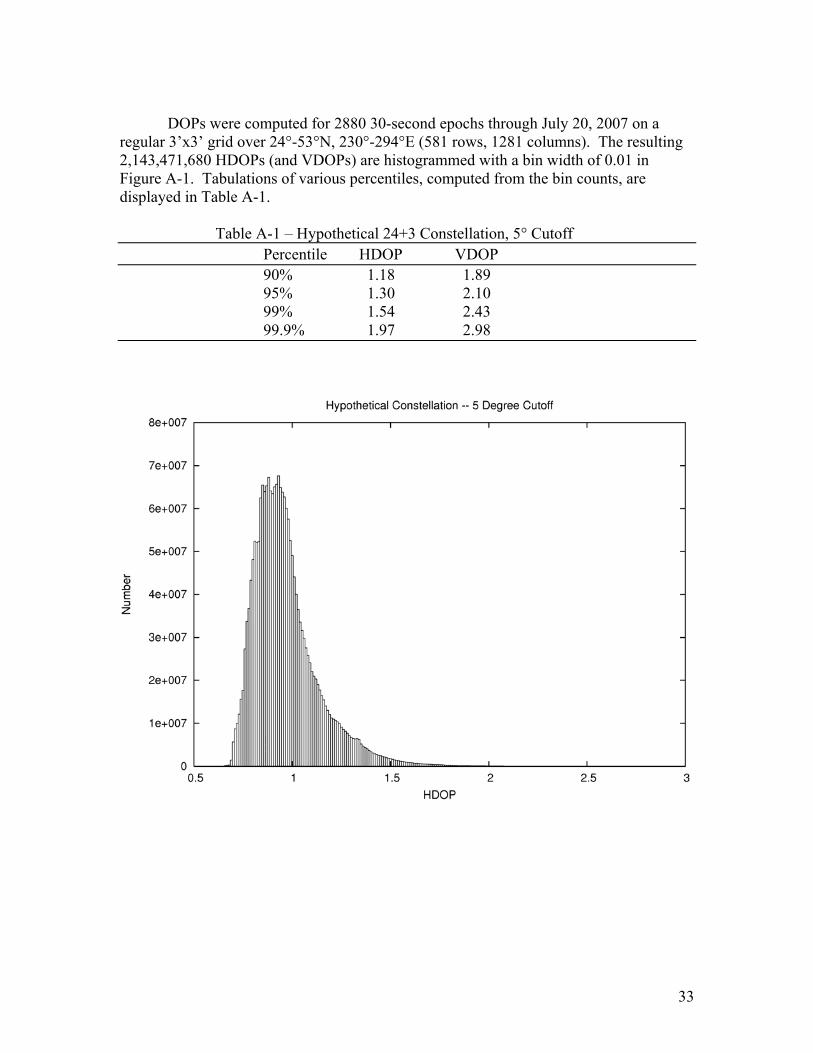
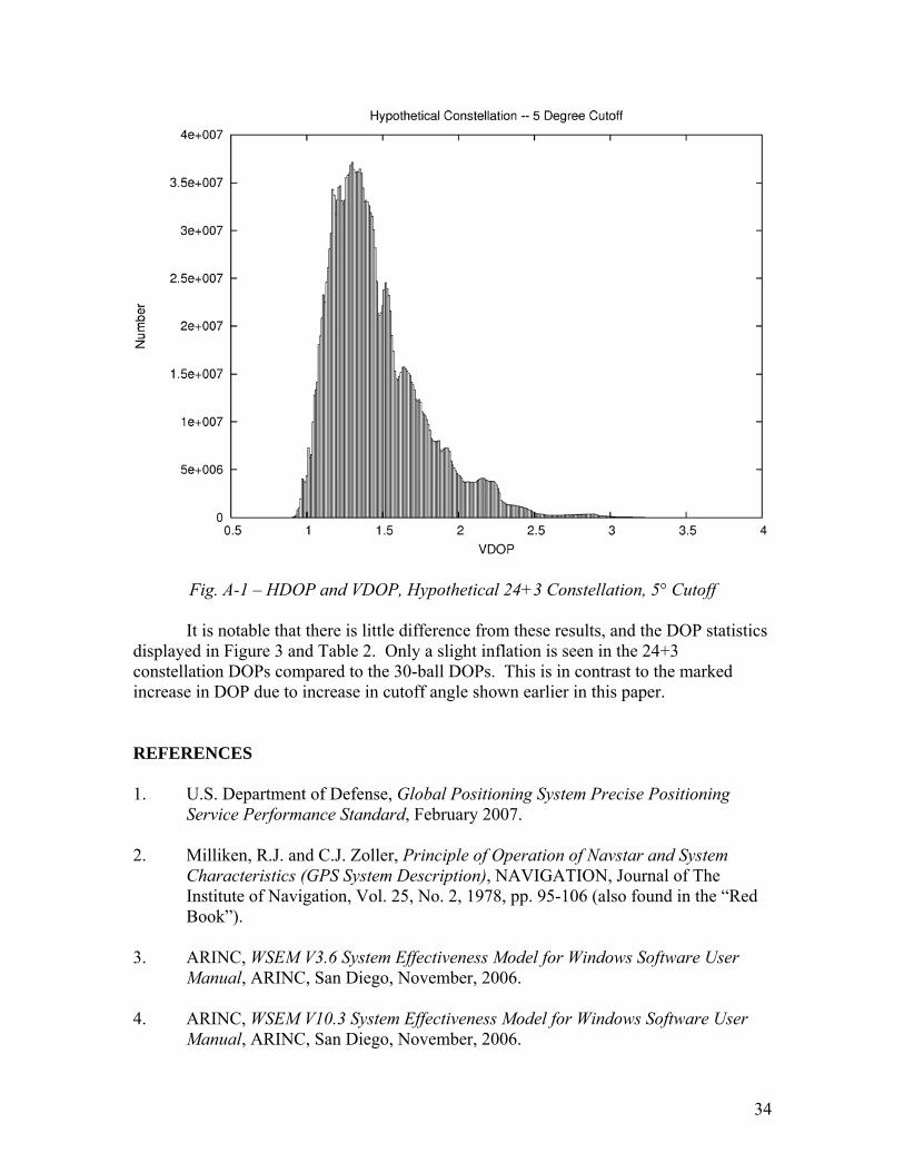
33

DOPs were computed for 2880 30-second epochs through July 20, 2007 on a regular 3’x3’ grid over 24°-53°N, 230°-294°E (581 rows, 1281 columns). The resulting 2,143,471,680 HDOPs (and VDOPs) are histogrammed with a bin width of 0.01 in Figure A-1. Tabulations of various percentiles, computed from the bin counts, are displayed in Table A-1. Table A-1 – Hypothetical 24+3 Constellation, 5° Cutoff Percentile HDOP VDOP

90% 1.18 1.89 95% 1.30 2.10

99% 1.54 2.43 99.9% 1.97 2.98

34

Fig. A-1 – HDOP and VDOP, Hypothetical 24+3 Constellation, 5° Cutoff It is notable that there is little difference from these results, and the DOP statistics displayed in Figure 3 and Table 2. Only a slight inflation is seen in the 24+3 constellation DOPs compared to the 30-ball DOPs. This is in contrast to the marked increase in DOP due to increase in cutoff angle shown earlier in this paper. REFERENCES 1. U.S. Department of Defense, Global Positioning System Precise Positioning

Service Performance Standard, February 2007. 2. Milliken, R.J. and C.J. Zoller, Principle of Operation of Navstar and System

Characteristics (GPS System Description), NAVIGATION, Journal of The Institute of Navigation, Vol. 25, No. 2, 1978, pp. 95-106 (also found in the “Red Book”).

3. ARINC, WSEM V3.6 System Effectiveness Model for Windows Software User

Manual, ARINC, San Diego, November, 2006. 4. ARINC, WSEM V10.3 System Effectiveness Model for Windows Software User

Manual, ARINC, San Diego, November, 2006.

35

5. Conley, R., R. Cosentino, C. J. Hegarty, E. D. Kaplan, J. L. Leva, M. U. de Haag,

and K. Van Dyke, Performance of Stand-Alone GPS, in Understanding GPS Principles and Applications, E. D. Kaplan and C. J. Hegarty, Eds., pp. 301-378, Artech House, Norwood, Mass, USA, 2nd edition, 2006.

6. Collins, J.P. and R.B. Langley, The Residual Tropospheric Propagation Delay:

How Bad Can It Get?, 11th International Technical Meeting of the Institute of Navigation, Nashville, Tennessee, September 15-18, 1998.

7. National Satellite Test Bed/Wide Area Augmentation Test and Evaluation Team,

Global Positioning System (GPS) Standard Positioning Service (SPS) Performance Analysis Report, Report #58, Federal Aviation Administration William J. Hughes Technical Center, Atlantic City International Airport, New Jersey, http://www.nstb.tc.faa.gov/DisplayArchive.htm, July 31, 2007 (issued quarterly).

8. Conley, R., GPS Performance: What Is Normal?, NAVIGATION, Journal of The

Institute of Navigation, Vol. 40, No. 3, 1993, pp. 261-81. 9. GPS Support Center, How Dangerous Is It To Use a Single Point Prediction for

an Entire Region?, http://web.archive.org/web/20040511160956/www.schriever.af.mil/gpssupportcenter/archive/Frontpage/J286PointVsGrid.htm, October 12, 2000.

10. Greenspan, R. L., A. K. Tetwsky, J. I. Donna, and J. A. Klobuchar, The Effects of

Ionospheric Errors on Single-Frequency GPS Users, Proceedings of the 4th International Technical Meeting of the Satellite Division of the Institute of Navigation ION GPS 1991, Albuquerque, New Mexico, pp. 291-298, September 11-13, 1991.

11. McDonald, K. D. and C. J. Hegarty, Post-Modernization GPS Performance

Capabilities, Proceedings of the IAIN World Congress and the 56th Annual Meeting of the Institute of Navigation, San Diego, California, pp. 242-249, June 26-28, 2000.

12. GPS Joint Program Office, Navstar Global Positioning System Interface

Specification, IS-GPS-200D, El Segundo, CA, March 2006. 13. Milbert, D., GPS Accuracy Monitor (Garmin 12XL),

http://home.comcast.net/~dmilbert/handacc/accur.htm, 2001, updated August 9, 2005.

14. RTCA, Inc., DO-229D, Minimum Operational Performance Standards for Global

Positioning System/Wide Area Augmentation System Airborne Equipment, SC-169, RTCA, Inc., Washington D.C., 2006.

36

15. Black, H.D. and A. Eisner, Correcting Satellite Doppler Data for Tropospheric

Effects, Journal of Geophysical Research, Vol. 89, D2, 1984, pp. 2616-26. 16. Klobuchar, John A., Ionospheric Time-Delay Algorithm for Single-Frequency

GPS Users, IEEE Transactions on Aerospace and Electronic Systems, Vol. AES-23, No. 3, May 1987, p. 325-331.

17. Komjathy, A., Global Ionospheric Total Electron Content Mapping Using the

Global Positioning System, Ph.D. dissertation, Department of Geodesy and Geomatics Engineering Technical Report No. 188, University of New Brunswick, Fredericton, New Brunswick, Canada, September 1997.

18. Forsythe, G.E., M.A. Malcolm, and C.B. Moler, Computer Methods for

Mathematical Computations, Prentice-Hall, Englewood Cliffs, New Jersey, 1977. 19. Press, W.H., S.A. Teukolsky, W.A. Vetterling, B.P. Flannery, Numerical Recipies

in Fortran 77, Second Ed., Cambridge University Press, New York., 1992. 20. Leandro, R., M. Santos, and R.B. Langley, UNB Neutral Atmosphere Models:

Development and Performance, Proceedings of the 2006 National Technical Meeting of the Institute of Navigation, Monterey, California, pp. 564-73, January 18-20, 2006.

21. Niell, A.E., Global Mapping Functions for the Atmosphere Delay at Radio

Wavelengths, Journal of Geophysical Research, Vol. 101, No. B2, pp. 3227-46, 1996.

22. GPS Operations Center, GPS Operations Center Archived File Retrieval,

http://gps.afspc.af.mil/gpsoc/archive, 2007 (updated daily). 23. International GNSS Service (IGS), web site and electronic products,

http://igscb.jpl.nasa.gov/. 24. National Geodetic Survey (NGS), web site and electronic products,

http://www.ngs.noaa.gov/. 25. Center for Orbit Determination in Europe (CODE), web site and electronic

products, http://www.aiub.unibe.ch/content/research/gnss/code___research/index_eng.html.

26. NOAA Space Environment Center, Real-time US-Total Electron Content:

Vertical and Slant, http://www.sec.noaa.gov/ustec/index.html, 2007 (updated every 15 minutes).

27. Ghoddousi-Fard, R., Online Raytracing, Department of Geodesy and Geomatics

37

Engineering, University of New Brunswick, Fredericton, New Brunswick, Canada, http://galileo.gge.unb.ca/main.shtml, 2007.

28. NOAA Global Systems Division, Ground-Based GPS Meteorology (GPS-MET),

http://www.gpsmet.noaa.gov/jsp/index.jsp, 2007.