Embed Size (px)
Citation preview
DIGITAL VIDEO IMAGE QUALITY ANDPERCEPTUAL CODING
H. R. Wu K. R. Rao
Royal Melbourne Institute of Technology, University of Texas at Arlington,
Australia USA

To those who have pioneered, inspired and persevered.
Contents
List of Figures iii
List of Tables vi
2 Fundamentals of Human Vision and Vision Modeling 1
2.1 Introduction . . . . . . . . . . . . . . . . . . . . . . . . . . . . . . . . 1
2.2 A Brief Overview of the Visual System . . . . . . . . . . . . . . . . . 2
2.3 Color Vision . . . . . . . . . . . . . . . . . . . . . . . . . . . . . . . . 4
2.3.1 Colorimetry . . . . . . . . . . . . . . . . . . . . . . . . . . . . 4
2.3.2 Color Appearance, Color Order Systems, and Color Difference . 8
2.4 Luminance and the Perception of Light Intensity . . . . . . .. . . . . . 12
2.4.1 Luminance . . . . . . . . . . . . . . . . . . . . . . . . . . . . 12
2.4.2 Perceived Intensity . . . . . . . . . . . . . . . . . . . . . . . . 14
2.5 Spatial Vision and Contrast Sensitivity . . . . . . . . . . . . .. . . . . 17
2.5.1 Acuity and Sampling . . . . . . . . . . . . . . . . . . . . . . . 17
2.5.2 Contrast Sensitivity . . . . . . . . . . . . . . . . . . . . . . . . 18
2.5.3 Multiple Spatial Frequency Channels . . . . . . . . . . . . . .20
2.5.3.1 Pattern adaptation . . . . . . . . . . . . . . . . . . . 21
2.5.3.2 Pattern detection . . . . . . . . . . . . . . . . . . . . 22
2.5.3.3 Masking and facilitation . . . . . . . . . . . . . . . . 23
2.5.3.4 Nonindependence in spatial frequency and orientation 25
i
2.5.3.5 Chromatic contrast sensitivity . . . . . . . . . . . . . 26
2.5.3.6 Suprathreshold contrast sensitivity . . . . . . . . . . 28
2.5.3.7 Image compression and image difference . . . . . . . 31
2.6 Temporal Vision and Motion . . . . . . . . . . . . . . . . . . . . . . . 32
2.6.1 Temporal CSF . . . . . . . . . . . . . . . . . . . . . . . . . . 32
2.6.2 Apparent Motion . . . . . . . . . . . . . . . . . . . . . . . . . 35
2.7 Visual Modeling . . . . . . . . . . . . . . . . . . . . . . . . . . . . . . 37
2.7.1 Image and Video Quality Research . . . . . . . . . . . . . . . . 38
2.8 Conclusions . . . . . . . . . . . . . . . . . . . . . . . . . . . . . . . . 39
Index 46
ii
List of Figures
2.1 Maxwell diagram representing the concept of color-matching with threeprimaries, R, G, and B. . . . . . . . . . . . . . . . . . . . . . . . . . . 5
2.2 The CIE 1931 2◦ Standard Observer System of Colorimetry. A) (Topleft) The color-matching functions based on real primariesR, G, and B.B) (Top right) The transformed color-matching functions for the imagi-nary primaries, X, Y,and Z. C) (Bottom) The (x, y) chromaticity diagram. 7
2.3 The organization of the Munsell Book of Colors. A) (Left)Arrangementof the hues in a plane of constant value. B) (Right) A hue leaf withvariation in value and chroma. . . . . . . . . . . . . . . . . . . . . . . 9
2.4 A CRT gamut plotted in CIELAB space. . . . . . . . . . . . . . . . . . 11
2.5 TheHelmholtz-Kohlrausch effect in which the apparent brightness ofisoluminant chromatic colors increases with chroma. The loci of con-stant ratios of the luminance of chromatic colors to a white reference(B/L) based on heterochromatic brightness matches of Sanders and Wyszecki[?, ?] are shown in the CIE 1964 (x10, y10) chromaticity diagram. From [?]. 13
2.6 A variety of luminance versus lightness functions: 1) Munsell renotationsystem, observations on a middle-gray background; 2) Original Mun-sell system, observations on a white background; 3) Modifiedversionof (1) for a middle-gray background; 4) CIE L∗ function, middle-graybackground; 5) Gray scale of theColor Harmony Manual, backgroundsimilar to the grays being compared; 6) Gray scale of theDIN ColorChart, gray background. Equations from [?]. . . . . . . . . . . . . . . . 16
2.7 Various lightness illusions. A) Simultaneous contrast: The appearanceof the identical gray squares changes due to the background.B) Crispen-ing: The difference between the two gray squares is more perceptiblewhen the background is close to the lightness of the squares.C) White’sillusion: The appearance of the identical gray bars changeswhen theyare embedded in the white and black stripes. . . . . . . . . . . . . . .. 17
iii
2.8 Contrast sensitivity function for different mean luminance levels. Thecurves were generated using the empirical model of the achromatic CSFin [?]. . . . . . . . . . . . . . . . . . . . . . . . . . . . . . . . . . . . 19
2.9 The contrast sensitivity function represented as the envelope of multiple,more narrowly tuned spatial frequency channels. . . . . . . . . .. . . 21
2.10 Pattern and orientation adaptation. A) After adaptingto the two patternson the left by staring at the fixation bar in the center for a minute orso, the two identical patterns in the center will appear to have differentwidths. Similarly, adaptation to the tilted patterns on theright will causean apparent orientation change in the central test patterns. B) Adaptationto a specific spatial frequency (arrow) causes a transient loss in contrastsensitivity in the region of the adapting frequency and a dipin the CSF. 22
2.11 Contrast masking experiment showing masking and facilitation by themasking stimulus. The threshold contrasts (ordinate) for detecting a 2cpd target grating are plotted as a function of the contrast of a superim-posed masking grating. Each curve represents the results for a mask ofa different spatial frequency. Mask frequencies ranged from 1 to 4 cpd.The curves are displaced vertically for clarity. The dashedlines indicatethe unmasked contrast threshold. From [?]. . . . . . . . . . . . . . . . 24
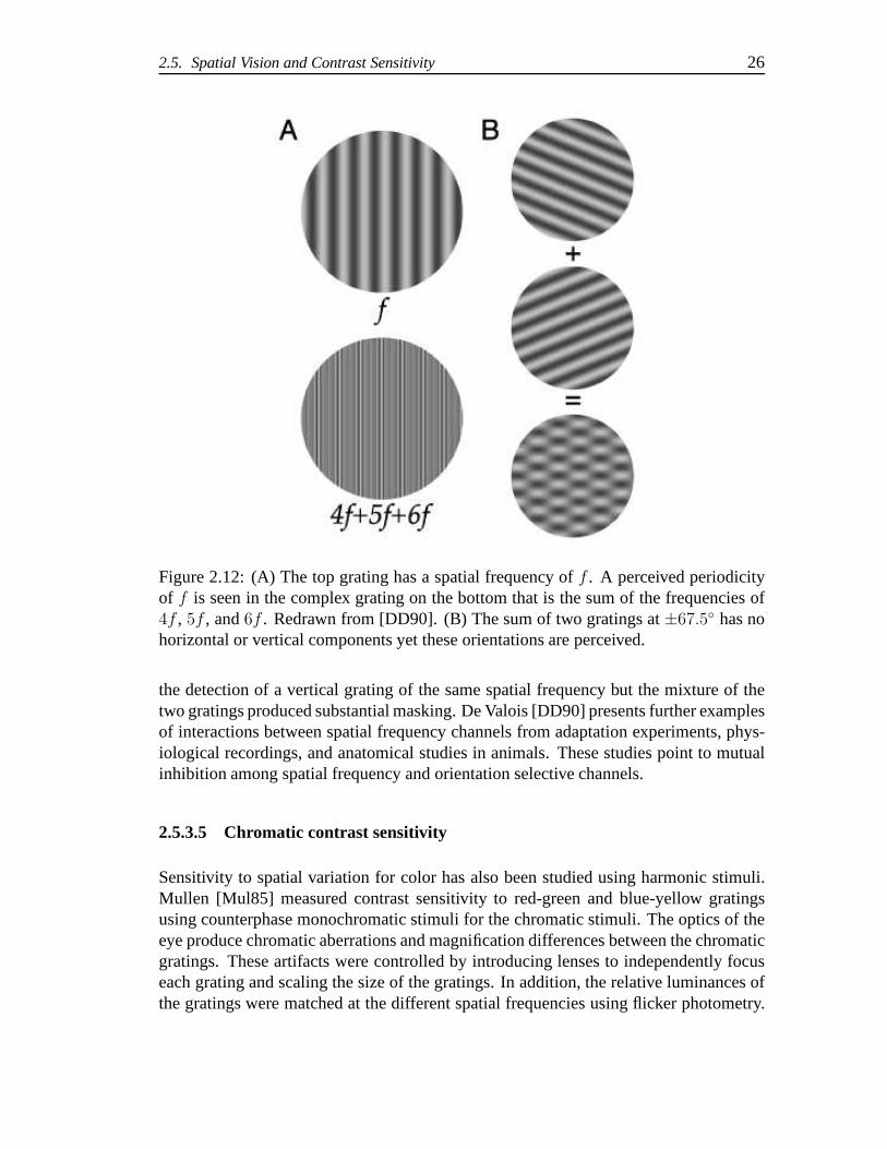
2.12 (A) The top grating has a spatial frequency off . A perceived periodicityof f is seen in the complex grating on the bottom that is the sum of thefrequencies of4f , 5f , and6f . Redrawn from [?]. (B) The sum of twogratings at±67.5◦ has no horizontal or vertical components yet theseorientations are perceived. . . . . . . . . . . . . . . . . . . . . . . . . 26
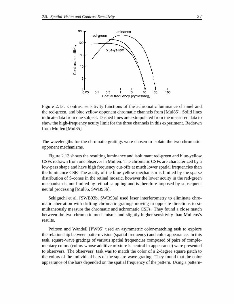
2.13 Contrast sensitivity functions of the achromatic luminance channel andthe red-green, and blue yellow opponent chromatic channelsfrom [?].Solid lines indicate data from one subject. Dashed lines areextrapolatedfrom the measured data to show the high-frequency acuity limit for thethree channels in this experiment. Redrawn from Mullen [?].. . . . . . 27
2.14 Results from Georgeson and Sullivan [?] showing equal-contrast con-tours for suprathreshold gratings of various spatial frequencies matchedto 5 cpd gratings. . . . . . . . . . . . . . . . . . . . . . . . . . . . . . 29
iv
2.15 (A) Contrast matches between stimuli that vary in different dimensionsof color space: luminance (lum), isoluminant red-green (LM), isolumi-nant blue-yellow (S), L-cone excitation only (L), and M-cone excita-tion only (M). The data show proportionality in contrast matches (solidlines). The dashed lines, slope equals 1, indicate the prediction for con-trast based on equal cone contrast. (B) Average contrast-matching ratiosacross observers for the different pairwise comparisons ofcontrast. Di-amonds indicate individual observers’ ratios. A ratio of 1 (dashed line)indicates prediction based on cone-contrast. From [?]. . . . . . . . . . . 30
2.16 Temporally counterphase modulated gratings change contrast over timesinusoidally producing a pattern that flickers. Each plot onthe left showsthe amplitude at a point in time. The luminance profile is simulated onthe right. . . . . . . . . . . . . . . . . . . . . . . . . . . . . . . . . . . 33
2.17 (A) Temporal CSF as a function of mean luminance for a large flickeringfield. (B) The data in A are replotted in terms of amplitude rather thancontrast. Replotted from [?]. . . . . . . . . . . . . . . . . . . . . . . . 34
2.18 (A) Spatial contrast sensitivity measured for gratings modulated at vari-ous temporal frequencies. (B) Temporal contrast sensitivity for gratingsof various spatial frequencies. The mean luminance was heldconstantat 20 cd/m2. From [?]. . . . . . . . . . . . . . . . . . . . . . . . . . . 35
2.19 A representation of a spatiotemporal contrast sensitivity surface. Re-drawn from [?]. . . . . . . . . . . . . . . . . . . . . . . . . . . . . . . 36
v

List of Tables
vi
Chapter 2
Fundamentals of Human Vision andVision Modeling
Ethan D. Montag and Mark D. FairchildRochester Institute of Technology, Rochester, New York
2.1 Introduction
Just as the visual system evolved to best adapt to the environment, video displays andvideo encoding technology is evolving to meet the requirements demanded by the vi-sual system. If the goal of video display is to veridically reproduce the world as seenby the mind’s eye, we need to understand the way the visual system itself representsthe world. This understanding involves finding the answer toquestions such as: Whatcharacteristics of a scene are represented in the visual system? What are the limits ofvisual perception? What is the sensitivity of the visual system to spatial and temporalchange? How does the visual system encode color information?
In this chapter, the limits and characteristics of human vision will be introduced inorder to elucidate a variety of the requirements needed for video display. Through anunderstanding of the fundamentals of vision, not only can the design principles for videoencoding and display be determined but methods for their evaluation can be established.That is, not only can we determine what is essential to display and how to display it,but we can also decide on the appropriate methods to use to measure the quality ofvideo display in terms relevant to human vision. In addition, an understanding of the
2.2. A Brief Overview of the Visual System 2
visual system can lead to insight into how rendering video imagery can be enhanced foraesthetic and scientific purposes.
2.2 A Brief Overview of the Visual System
Our knowledge of how the visual system operates derives frommany diverse fields rang-ing from anatomy and physiology to psychophysics and molecular genetics, to name afew. The physical interaction of light with matter, the electro-chemical nature of nerveconduction, and the psychology of perception all play a role. In his Treatise on Phys-iological Optics [vH11], Helmholtz divides the study of vision into three parts: 1) thetheory of the path of light in the eye, 2) the theory of the sensations of the nervous mech-anisms of vision, and 3) the theory of the interpretation of the visual sensations. Herewe will briefly trace the visual pathway to summarize its parts and functions.
Light first encounters the eye at the cornea, the main refractive surface of the eye.The light then enters the eye through the pupil, the hole in the center of the circularpigmented iris, which gives our eyes their characteristic color. The iris is bathed inaqueous humor, the watery fluid between the cornea and lens ofthe eye. The pupildiameter, which ranges from about 3 to 7 mm, changes based on the prevailing light leveland other influences of the autonomic nervous system. The constriction and dilation ofthe pupil changes its area by a factor of 5, which as we will seelater contributes littleto the ability of the eye to adapt to the wide range of illumination it encounters. Thelight then passes through the lens of the eye, a transparent layered body that changesshape with accommodation to focus the image on the back of theeye. The main body ofthe eyeball contains the gelatinous vitreous humor maintaining the eye’s shape. Liningthe back of the eye is the retina, where the light sensitive photoreceptors transduce theelectromagnetic energy of light into the electro-chemicalsignals used by the nervoussystem. Behind the retina is the pigment epithelium that aids in trapping the light that isnot absorbed by the photoreceptors and provides metabolic activities for the retina andphotoreceptors.
An inverted image of the visual field is projected onto the retina. The retina is consid-ered an extension of the central nervous system and in fact develops as an outcropping ofthe neural tube during embryonic development. It consists of five main neural cell typesorganized into three cellular layers and two synaptic layers. The photoreceptors, spe-cialized neurons that contain photopigments that absorb and initiate the neural responseto light, are located on the outer part of the retina meaning that light must pass throughall the other retinal layers before being detected. The signals from the photoreceptorsare processed via the multitude of retinal connections and eventually exit the eye by wayof the optic nerve, the axons of the ganglion cells, which make up the inner cellular layerof the retina. These axons are gathered together and exit theeye at the optic disc formingthe optic nerve that projects to the lateral geniculate nucleus, a part of the thalamus in
2.2. A Brief Overview of the Visual System 3
the midbrain. From here, there are synaptic connections to neurons that project to theprimary visual cortex located in the occipital lobe of the cerebral cortex. The humancortex contains many areas that respond to visual stimuli (covering 950 cm2 or 27% ofthe cortical surface [Ess03]) where processing of the various modes of vision such asform, location, motion, color, etc. occur. It is interesting to note that these various areasmaintain a spatial mapping of the visual world even as the responses of neurons becomemore complex.
There are two classes of photoreceptors, rods and cones. Therods are used for visionat very low light levels (scotopic) and do not normally contribute to color vision. Thecones, which operate at higher light levels (photopic), mediate color vision and the see-ing of fine spatial detail. There are three types of cones known as the short wavelengthsensitive cones (S-cones), the middle wavelength sensitive cones (M-cones), and thelong wavelength sensitive cones (L-cones), where the wavelength refers to the visibleregion of the spectrum between approximately 400 - 700 nm. Each cone type is color-blind; that is, the wavelength information of the light absorbed is lost. This is knownas the Principle of Univariance so that the differential sensitivity to wavelength by thephotoreceptors is due to the probability of photon absorption. Once a photopigmentmolecule absorbs a photon, the effect on vision is the same regardless of the wavelengthof the photon. Color vision derives from the differential spectral sensitivities of thethree cone types and the comparisons made between the signals generated in each conetype. Because there are only three cone types, it is possibleto specify the color stimulusin terms of three numbers indicating the absorption of lightby each of the three conephotoreceptors. This is the basis of trichromacy, the ability to match any color with amixture of three suitably chosen primaries.
As an indication of the processing in the retina, we can note that there are approx-imately 127 million receptors (120 million rods and 7 million cones) in the retina yetonly 1 million ganglion cells in the optic nerve. This overall 127:1 convergence of in-formation in the retina belies the complex visual processing in the retina. For scotopicvision there is convergence, or spatial summation, of 100 receptors to 1 ganglion cell toincrease sensitivity at low light levels. However, in the rod-free fovea, cone receptorsmay have input to more than one ganglion cell. The locus of light adaptation is sub-stantially retinal and the center-surround antagonistic receptive field properties of theganglion cells, responsible for the chromatic-opponent processing of color and lateralinhibition, are due to lateral connections in the retina.
Physiological analysis of the receptive field properties ofneurons in the cortex hasrevealed a great deal of specialization and organization intheir response in different re-gions of the cortex. Neurons in the primary visual cortex, for example, show responsesthat are tuned to stimuli of specific sizes and orientations (see [KNM84]). The area MT,located in the medial temporal region of the cortex in the macaque monkey, is area inwhich the cells are remarkably sensitive to motion stimuli [MM93]. Damage to homol-ogous areas in humans (through stroke or accident, for example) has been thought to
2.3. Color Vision 4
cause defects in motion perception [Zek91]. Deficits in other modes of vision such ascolor perception, localization, visual recognition and identification, have been associ-ated with particular areas or processing streams within thecortex.
2.3 Color Vision
As pointed out by Newton, color is a property of the mind and not of objects in theworld. Color results from the interaction of a light source,an object, and the visualsystem. Although the product of the spectral radiance of a source and the reflectance ofan object (or the spectral distribution of an emissive source such as an LCD or a CRTdisplay) specify the spectral power distribution of the distal stimulus to color vision,the color signal can be considered the product of this signalwith the spectral sensitivityof the three cone receptor types. The color signal can therefore be summarized as 3numbers that express the absorption of the three cone types at each “pixel” in the scene.Unfortunately, a standard for specifying cone signals has not yet been agreed upon, butthe basic principles of color additivity have led to a description of the color signal thatcan be considered as linearly related to the cone signals.
2.3.1 Colorimetry
Trichromacy leads to the principle that any color can be matched with a mixture of threesuitable chosen primaries. We can characterize an additivematch by using an equationsuch as:
C1 = r1R + g1G + b1B, (2.1)
where the Red, Green, and Blue primaries are mixed together to match an arbitrary testlight C by adjusting their intensities with the scalars r, g,and b. The amounts of eachprimary needed to make the match are known as the tristimulusvalues. The behav-ior of color matches follows the linear algebraic rules of additivity and proportionality(Grassmann’s laws) [WS82]. Therefore, given another match:
C2 = r2R + g2G + b2B, (2.2)
the mixture of lights C1 and C2 can be matched by adding the constituent match com-ponents:
C3 = C1 + C2 = (r1 + r2)R + (g1 + g2)G + (b1 + b2)B. (2.3)
Scaling the intensities of the lights retains the match (at photopic levels):
kC3 = kC1 + kC2. (2.4)
2.3. Color Vision 5
R
G B
0.2
0.4
0.6
0.8
0.2
0.4
0.6
0.8
0.2
0.4
0.6
0.8
C4
C1
M
Amt. of R
Am
t. of
GA
mt. of
B
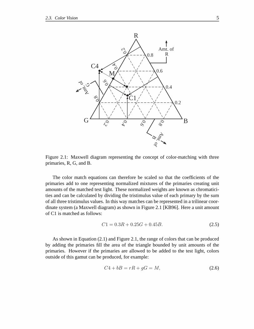
Figure 2.1: Maxwell diagram representing the concept of color-matching with threeprimaries, R, G, and B.
The color match equations can therefore be scaled so that thecoefficients of theprimaries add to one representing normalized mixtures of the primaries creating unitamounts of the matched test light. These normalized weightsare known as chromatici-ties and can be calculated by dividing the tristimulus valueof each primary by the sumof all three tristimulus values. In this way matches can be represented in a trilinear coor-dinate system (a Maxwell diagram) as shown in Figure 2.1 [KB96]. Here a unit amountof C1 is matched as follows:
C1 = 0.3R + 0.25G + 0.45B. (2.5)
As shown in Equation (2.1) and Figure 2.1, the range of colorsthat can be producedby adding the primaries fill the area of the triangle bounded by unit amounts of theprimaries. However if the primaries are allowed to be added to the test light, colorsoutside of this gamut can be produced, for example:
C4 + bB = rR + gG = M, (2.6)
2.3. Color Vision 6
where M is the color that appears in the matched fields. This can be rewritten as:
C4 = rR + gG − bB, (2.7)
where a negative amount of a primary means the primary is added to the test field. InFigure 2.1, an example is shown where:
C4 = 0.6R + 0.6G − 0.2B. (2.8)
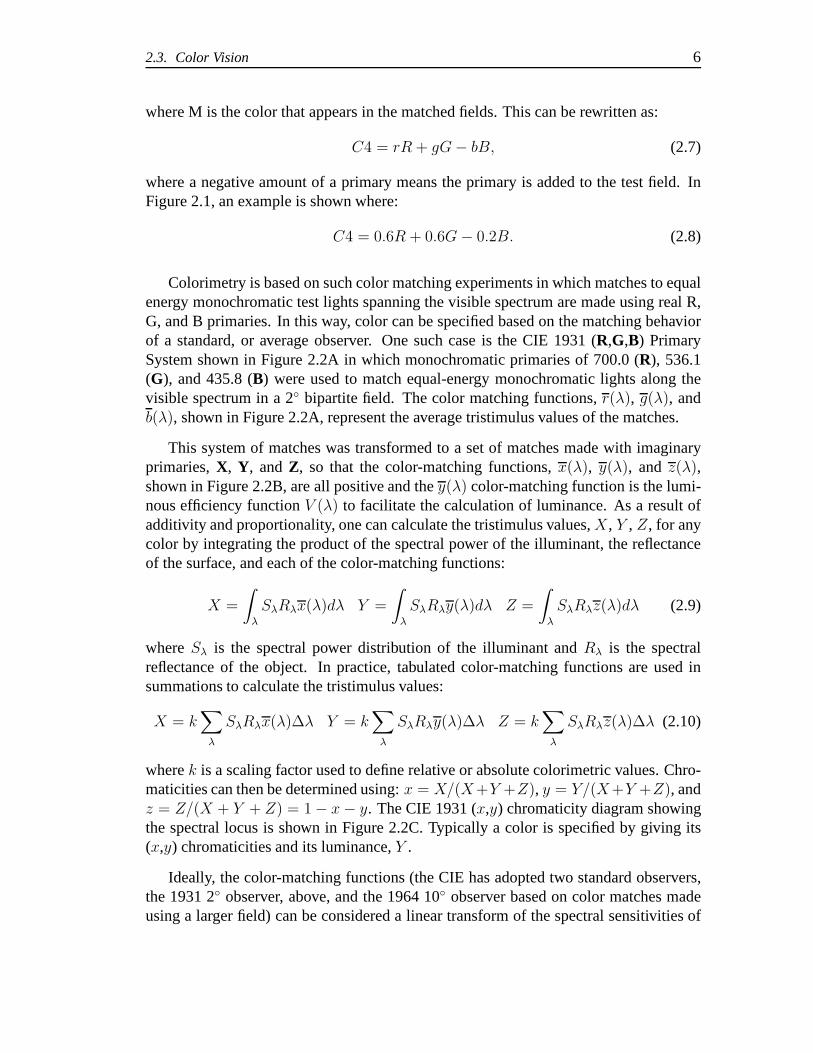
Colorimetry is based on such color matching experiments in which matches to equalenergy monochromatic test lights spanning the visible spectrum are made using real R,G, and B primaries. In this way, color can be specified based onthe matching behaviorof a standard, or average observer. One such case is the CIE 1931 (R,G,B) PrimarySystem shown in Figure 2.2A in which monochromatic primaries of 700.0 (R), 536.1(G), and 435.8 (B) were used to match equal-energy monochromatic lights along thevisible spectrum in a 2◦ bipartite field. The color matching functions,r(λ), g(λ), andb(λ), shown in Figure 2.2A, represent the average tristimulus values of the matches.
This system of matches was transformed to a set of matches made with imaginaryprimaries,X, Y, andZ, so that the color-matching functions,x(λ), y(λ), and z(λ),shown in Figure 2.2B, are all positive and they(λ) color-matching function is the lumi-nous efficiency functionV (λ) to facilitate the calculation of luminance. As a result ofadditivity and proportionality, one can calculate the tristimulus values,X, Y , Z, for anycolor by integrating the product of the spectral power of theilluminant, the reflectanceof the surface, and each of the color-matching functions:
X =
∫
λ
SλRλx(λ)dλ Y =
∫
λ
SλRλy(λ)dλ Z =
∫
λ
SλRλz(λ)dλ (2.9)
whereSλ is the spectral power distribution of the illuminant andRλ is the spectralreflectance of the object. In practice, tabulated color-matching functions are used insummations to calculate the tristimulus values:
X = k∑
λ
SλRλx(λ)∆λ Y = k∑
λ
SλRλy(λ)∆λ Z = k∑
λ
SλRλz(λ)∆λ (2.10)
wherek is a scaling factor used to define relative or absolute colorimetric values. Chro-maticities can then be determined using:x = X/(X+Y +Z), y = Y/(X+Y +Z), andz = Z/(X + Y + Z) = 1 − x − y. The CIE 1931 (x,y) chromaticity diagram showingthe spectral locus is shown in Figure 2.2C. Typically a coloris specified by giving its(x,y) chromaticities and its luminance,Y .
Ideally, the color-matching functions (the CIE has adoptedtwo standard observers,the 1931 2◦ observer, above, and the 1964 10◦ observer based on color matches madeusing a larger field) can be considered a linear transform of the spectral sensitivities of
2.3. Color Vision 7
0 0.1 0.2 0.3 0.4 0.5 0.6 0.7 0.80
0.1
0.2
0.3
0.4
0.5
0.6
0.7
0.8
0.9
380
x
y
450
475
500
525
550
575
600
625650720
400 450 500 550 600 650 700−0.1
0.0
0.1
0.2
0.3
Wavelength, nm
Tris
timul
us V
alue
s
435.
8 nm
546.
1 nm
700.
0 nm
_b
_g
_r
400 450 500 550 600 650 7000
0.5
1
1.5
2
Wavelength, nm
Tris
timul
us V
alue
s
_z
_y
_x
Figure 2.2: The CIE 1931 2◦ Standard Observer System of Colorimetry. A) (Top left)The color-matching functions based on real primaries R, G, and B. B) (Top right) Thetransformed color-matching functions for the imaginary primaries, X, Y,and Z. C) (Bot-tom) The (x, y) chromaticity diagram.
the L-, M-, and S- cones. It is therefore possible to specify color in terms of L-, M- andS-cone excitation.
Currently, work is underway to reconcile the data from colormatching, luminousefficiency, and spectral sensitivity into a system that can be adopted universally. Un-til recently, specification of the cone spectral sensitivities has been a difficult problembecause the overlap of their sensitivities makes it difficult to isolate these functions. Asystem of colorimetry based on L, M, and S primaries would allow a more direct and in-tuitive link between color specification and the early physiology of color vision [Boy96].
2.3. Color Vision 8
2.3.2 Color Appearance, Color Order Systems, and Color Differ-ence
A chromaticity diagram is useful for specifying color and determining the results ofadditive color mixing. However, it gives no insight into theappearance of colors. Theappearance of a particular color depends on the viewer’s state of adaptation, both glob-ally and locally, the size, configuration, and location of the stimulus in the visual field,the color and location of other objects in the scene, the color of the background and sur-round, and even the colors of objects presented after the onein question. Therefore, twocolored patches with the same chromaticity and luminance may have wildly differentappearances.
Although color is typically thought of as being three-dimensional due to the trichro-matic nature of color matching, five perceptual attributes are needed for a completespecification of color appearance [Fai98]. These are:brightness, the attribute accordingto which an area appears to be more or less intense;lightness, the brightness of an arearelative to a similarly illuminated area that appears to be white; colorfulness (chromat-icness), the attribute according to which an area appears to be moreor less chromatic;chroma, the colorfulness of an area relative to a similarly illuminated area that appearsto be white; andhue, the attribute of a color denoted by its name such as blue, green,yellow, orange, etc. One other common attribute, saturation, defined as the colorfulnessof an area relative to its brightness, is redundant when these five attributes are specified.Brightness and colorfulness are considered sensations that indicate the absolute levelsof the corresponding sensations while lightness and chromaindicate the relative lev-els of these sensations. In general, increasing the illumination increases the brightnessand colorfulness of a stimulus while the lightness and chroma remain approximatelyconstant. Therefore a video or photographic reproduction of a scene can maintain therelative attributes even though the absolute levels of illumination are not realizable.
In terms of hue, it is observed that the colors red, green, yellow, and blue, are uniquehues that do not have the appearance of being mixtures of other hues. In addition, theyform opponent pairs so that perception of red and green cannot coexist in the same stim-ulus nor can yellow and blue. In addition, these terms are sufficient for describing thehue components of any unrelated color stimulus. This idea ofopponent channels, firstascribed to Hering [Her64], indicates a higher level of visual processing concerned withthe organization of color appearance. Color opponency is observed both physiologi-cally and psychophysically in the chromatic channels with L- and M-cone (L-M) oppo-nency and opponency between S-cones and the sum of the L- and M-cones (S-(L+M)).However, although these chromatic mechanisms are sure to bethe initial substrate ofred-green and yellow-blue opponency, they do not account for the phenomenology ofHering’s opponent hues.
Even under standard viewing conditions of adaptation and stimulus presentation,
2.3. Color Vision 9
5R 10R
5YR
10YR
5Y
10Y
5GY
10GY
5G
10G5GB
5B
10B
5PB
10PB
5P
10P
5RP10RP
10GB
1 2 3 46
78
9
/2/4
/6/8
/10
Boundary of colorant mixturegamut
Munsell chroma
Mun
sell
valu
e
Black
White
0/
1/
2/
3/
4/
5/
6/
7/
8/
9/
10/
/2 /4 /6 /8 /10
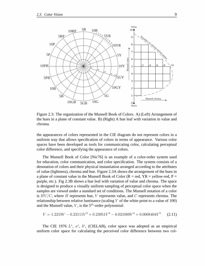
Figure 2.3: The organization of the Munsell Book of Colors. A) (Left) Arrangement ofthe hues in a plane of constant value. B) (Right) A hue leaf with variation in value andchroma.
the appearances of colors represented in the CIE diagram do not represent colors in auniform way that allows specification of colors in terms of appearance. Various colorspaces have been developed as tools for communicating color, calculating perceptualcolor difference, and specifying the appearance of colors.
The Munsell Book of Color [Nic76] is an example of a color-order system usedfor education, color communication, and color specification. The system consists of adenotation of colors and their physical instantiation arranged according to the attributesof value (lightness), chroma and hue. Figure 2.3A shows the arrangement of the hues ina plane of constant value in the Munsell Book of Color (R = red,YR = yellow-red, P =purple, etc.). Fig 2.3B shows a hue leaf with variation of value and chroma. The spaceis designed to produce a visually uniform sampling of perceptual color space when thesamples are viewed under a standard set of conditions. The Munsell notation of a coloris HV/C, whereH represents hue,V represents value, andC represents chroma. Therelationship between relative luminance (scalingY of the white point to a value of 100)and the Munsell value,V , is the 5th-order polynomial:
Y = 1.2219V − 0.23111V 2 + 0.23951V 3− 0.021009V 4 + 0.0008404V 5 (2.11)
The CIE 1976L∗, a∗, b∗, (CIELAB), color space was adopted as an empiricaluniform color space for calculating the perceived color difference between two col-
2.3. Color Vision 10
ors [CIE86]. The Cartesian coordinates,L∗, a∗, and b∗, of a color correspond to alightness dimension and two chromatic dimensions that are roughly red-green and blue-yellow. The coordinates of color are calculated from its tristimulus values and the tris-timulus values of a reference white so that the white is plotted atL∗ = 100, a∗ = 0,andb∗ = 0. The space is organized so that the polar transformations ofthea∗ andb∗
coordinates give the chroma,C∗
ab, and the hue angle,hab, of a color. The equations forcalculating CIELAB coordinates are:
L∗ = 116(Y/Yn)1/3
− 16a∗ = 500[(X/Xn)
1/3− (Y/Yn)
1/3]b∗ = 200[(Y/Yn)
1/3− (Z/Zn)
1/3]C∗
ab = [a∗2− b∗2]1/2
hab = arctan( b∗
a∗)
(2.12)
where (X,Y ,Z) are the color’s CIE tristimulus values and (Xn, Yn, Zn) are the tristim-ulus values of a reference white. For values ofY/Yn, X/Xn, andZ/Zn less than 0.01the formulae are modified (see [WS82] for details). Lightness, L∗, is an exponentialfunction of luminance. There is also an “opponent-like” transform for calculatinga∗
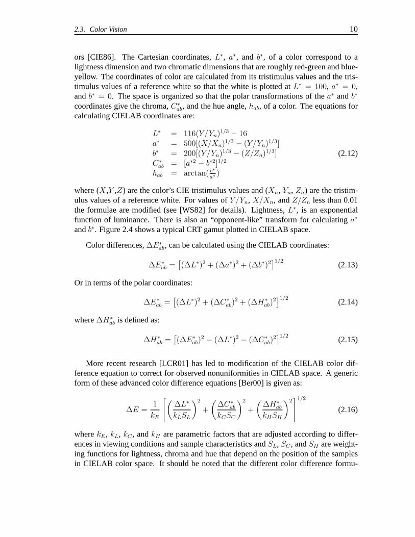
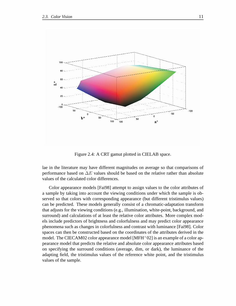
andb∗. Figure 2.4 shows a typical CRT gamut plotted in CIELAB space.
Color differences,∆E∗
ab, can be calculated using the CIELAB coordinates:
∆E∗
ab =[
(∆L∗)2 + (∆a∗)2 + (∆b∗)2]1/2
(2.13)
Or in terms of the polar coordinates:
∆E∗
ab =[
(∆L∗)2 + (∆C∗
ab)2 + (∆H∗
ab)2]1/2
(2.14)
where∆H∗
ab is defined as:
∆H∗
ab =[
(∆E∗
ab)2− (∆L∗)2
− (∆C∗
ab)2]1/2
(2.15)
More recent research [LCR01] has led to modification of the CIELAB color dif-ference equation to correct for observed nonuniformities in CIELAB space. A genericform of these advanced color difference equations [Ber00] is given as:
∆E =1
kE
[
(
∆L∗
kLSL
)2
+
(
∆C∗
ab
kCSC
)2
+
(
∆H∗
ab
kHSH
)2]1/2
(2.16)
wherekE, kL, kC , andkH are parametric factors that are adjusted according to differ-ences in viewing conditions and sample characteristics andSL, SC , andSH are weight-ing functions for lightness, chroma and hue that depend on the position of the samplesin CIELAB color space. It should be noted that the different color difference formu-
2.3. Color Vision 11
Figure 2.4: A CRT gamut plotted in CIELAB space.
lae in the literature may have different magnitudes on average so that comparisons ofperformance based on∆E values should be based on the relative rather than absolutevalues of the calculated color differences.
Color appearance models [Fai98] attempt to assign values tothe color attributes ofa sample by taking into account the viewing conditions underwhich the sample is ob-served so that colors with corresponding appearance (but different tristimulus values)can be predicted. These models generally consist of a chromatic-adaptation transformthat adjusts for the viewing conditions (e.g., illumination, white-point, background, andsurround) and calculations of at least the relative color attributes. More complex mod-els include predictors of brightness and colorfulness and may predict color appearancephenomena such as changes in colorfulness and contrast withluminance [Fai98]. Colorspaces can then be constructed based on the coordinates of the attributes derived in themodel. The CIECAM02 color appearance model [MFH+02] is an example of a color ap-pearance model that predicts the relative and absolute color appearance attributes basedon specifying the surround conditions (average, dim, or dark), the luminance of theadapting field, the tristimulus values of the reference white point, and the tristimulusvalues of the sample.
2.4. Luminance and the Perception of Light Intensity 12
2.4 Luminance and the Perception of Light Intensity
Luminance is a term that has taken on different meanings in different contexts and there-fore the concept of luminance, its definition, and its application can lead to confusion.Luminance is a photometric measure that has loosely been described as the “apparentintensity” of a stimulus but is actually defined as the effectiveness of lights of differentwavelengths in specific photometric matching tasks [SS99].The term is also used tolabel the achromatic channel of visual processing.
2.4.1 Luminance
The CIE definition of luminance [WS82] is a quantity that is a constant times the integralof the product of radiance andV (λ), the photopic spectral luminous efficiency function.V (λ) is defined as the ratio of radiant flux at wavelengthλm to that of wavelengthλ,when the two fluxes produce the same luminous sensations under specified conditionwith a value of1 at λm = 555 nm. Luminance efficiency is therefore tied to the tasksthat are used to measure it. Luminance is expressed in units of candelas per square meter(cd/m2). To control for the amount of light falling on the retina, the troland (td) unit isdefined as cd/m2 multiplied by the area of the pupil.
TheV (λ) function in use by the CIE was adopted by the CIE in 1924 and is basedon a weighted assembly of the results of a variety of visual brightness matching andminimum flicker experiments. The goal of theV (λ) in the CIE system of photome-try and colorimetry is to predict brightness matches so thatgiven two spectral powerdistributions,P1λ andP2λ, the expression:
∫
λ
P1λV (λ)dλ =
∫
λ
P2λV (λ)dλ (2.17)
predicts a brightness match and therefore additivity applies to brightness.
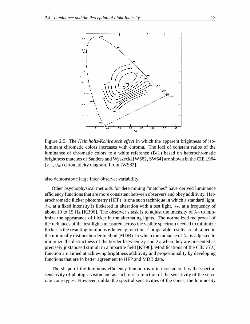
In direct heterochromatic brightness matching, it has beenshown that this additivitylaw, known as Abney’s law, fails substantially [WS82]. For example when a reference“white”, W, is matched in brightness to a “blue” stimulus,C1, and to a “yellow” stim-ulus, C2, the additive mixture ofC1 and C2 is found to be less bright than 2W, astimulus that is twice the radiance of the reference white [KB96]. Another example ofthe failure ofV (λ) to predict brightness matches is known as theHelmholtz-Kohlrauscheffect where chromatic stimuli of the same luminance as a referencewhite stimulus ap-pear brighter than the reference. In Figure 2.5, we see the results from Sanders andWyszecki [SW64] and presented in [WS82] that show how the ratio, B/L, of the lumi-nance of a chromatic test color, B, to the luminance of a whitereference,L, varies as afunction of chroma and hue. Direct hetereochromatic brightness matching experiments
2.4. Luminance and the Perception of Light Intensity 13
Figure 2.5: TheHelmholtz-Kohlrausch effect in which the apparent brightness of iso-luminant chromatic colors increases with chroma. The loci of constant ratios of theluminance of chromatic colors to a white reference (B/L) based on heterochromaticbrightness matches of Sanders and Wyszecki [WS82, SW64] areshown in the CIE 1964(x10, y10) chromaticity diagram. From [WS82].
also demonstrate large inter-observer variability.
Other psychophysical methods for determining “matches” have derived luminanceefficiency functions that are more consistent between observers and obey additivity. Het-erochromatic flicker photometry (HFP) is one such techniquein which a standard light,λS, at a fixed intensity is flickered in alteration with a test light, λT , at a frequency ofabout 10 to 15 Hz [KB96]. The observer’s task is to adjust the intensity ofλT to min-imize the appearance of flicker in the alternating lights. The normalized reciprocal ofthe radiances of the test lights measured across the visiblespectrum needed to minimizeflicker is the resulting luminous efficiency function. Comparable results are obtained inthe minimally distinct border method (MDB) in which the radiance ofλT is adjusted tominimize the distinctness of the border betweenλT andλS when they are presented asprecisely juxtaposed stimuli in a bipartite field [KB96]. Modifications of the CIEV (λ)function are aimed at achieving brightness additivity and proportionality by developingfunctions that are in better agreement to HFP and MDB data.
The shape of the luminous efficiency function is often considered as the spectralsensitivity of photopic vision and as such it is a function ofthe sensitivity of the sepa-rate cone types. However, unlike the spectral sensitivities of the cones, the luminosity
2.4. Luminance and the Perception of Light Intensity 14
function changes shape depending on the state of adaptation, especially chromatic adap-tation [SS99]. Therefore the luminosity function only defines luminance for the condi-tions under which it was measured. As measured by HFP and MDB,the luminosityfunction can be modeled as a weighted sum of L- and M-cone spectral sensitivities withL-cones dominating. The S-cones contribution to luminosity is considered negligibleunder normal conditions. (The luminosity function of dichromats, those color-deficientobservers who lack either the L- or M-cone photopigment, is the spectral sensitivity ofthe remaining longer wavelength sensitive receptor pigment. Protanopes, who lack theL-cone pigment, generally see “red” objects as being dark. Deuteranopes, who lack theM-cone pigment, see brightness similarly to color normal observers.)
2.4.2 Perceived Intensity
As the intensity of a background field increases, the intensity required to detect a thresh-old increment superimposed on the background increases. Weber’s law states that the ra-tio of the increment to the background or adaptation level isa constant so that∆I/I = k,whereI is the background intensity and∆I is the increment threshold (also known asthe just noticeable difference or JND) above this background level. Weber’s law is ageneral rule of thumb that applies across different sensorysystems.
To the extent that Weber’s Law holds, it states that threshold contrast is constant at alllevels of background adaptation so that a plot of∆I versus I will have a constant slope.In vision research, plots oflog(∆I) versuslog(I), known as threshold versus intensityor t.v.i. curves, exhibit a slope of one when Weber’s law applies. The curve that resultswhen the ratio,∆I/I, the Weber fraction, is plotted against background intensity has aslope of zero when Weber’s law applies.
The Weber fraction is a measure of contrast and it should be noted that contrastis a more important aspect of vision than the detection of absolute intensity. As theillumination on this page increases from dim illumination to full sunlight, the contrast ofthe ink to the paper remains constant even as the radiance of the reflected light off the inkin sunlight surpasses the radiance reflected off the white paper under dim illumination.
If the increment threshold is considered a unit of sensation, one can build a scale ofincreasing sensation by integrating JNDs so thatS = K log(I), whereS is the sensa-tion magnitude andK is a constant that depends on the particular stimulus conditions.The logarithmic relationship between stimulus intensity and the associated sensation isknown as Fechner’s Law. The increase in perceptual magnitude is characterized by acompressive relationship with intensity as shown in Figure2.6. Based on applicabilityof Weber’s law and the assumptions of Fechner’s Law, a scale of perceptual intensitycan be constructed based on the measurement of increment thresholds using classicalpsychophysical techniques to determine the Weber fraction.
2.4. Luminance and the Perception of Light Intensity 15
Weber’s law, in fact, does not hold for the full range of intensities that the visualsystem operates. However, at luminance levels above 100 cd/m2, typical of indoor light-ning, Weber’s Law holds fairly well. The value of the Weber fraction depends upon theexact stimulus configuration with a value as low as 1% under optimal conditions [HF86].In order to create a scale of sensation using Fechner’s Law, one would need to choosea Weber fraction that is representative of the conditions under which the scale would beused.
Logarithmic functions have been used for determining lightness differences such asin the BFD color difference equation [LR87]. It should be noted, however, that∆Evalues are typically larger than one JND. Since they do not represent true incrementthresholds, Weber’s law may not apply.
The validity of Fechner’s law has been questioned based on direct brightness scal-ing experiments using magnitude estimation techniques. Typically these experimentsyield scales of brightness that are power functions of the form S = kIa, whereS isthe sensation magnitude,I is the stimulus intensity,a is exponent that depends on thestimulus conditions, andk is a scaling constant. This relationship is known as Stevens’Power Law. For judgments of lightness, the exponent,a, typically has a value less thanone demonstrating a compressive relationship between stimulus intensity and perceivedmagnitude.
The value of the exponent is dependent on the stimulus conditions of the experimentused to measure it. Therefore, the choice of exponent must bebased on data fromexperiments that are representative of the conditions in which the law will be applied.As shown above, the Munsell Book of Color, Equation (2.11), and the L∗ function inCIELAB, Equation (2.12) are both exponential functions.
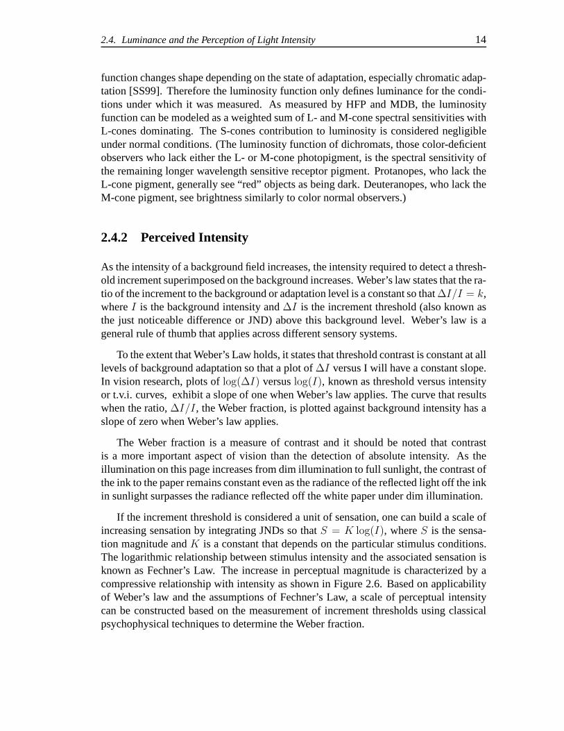
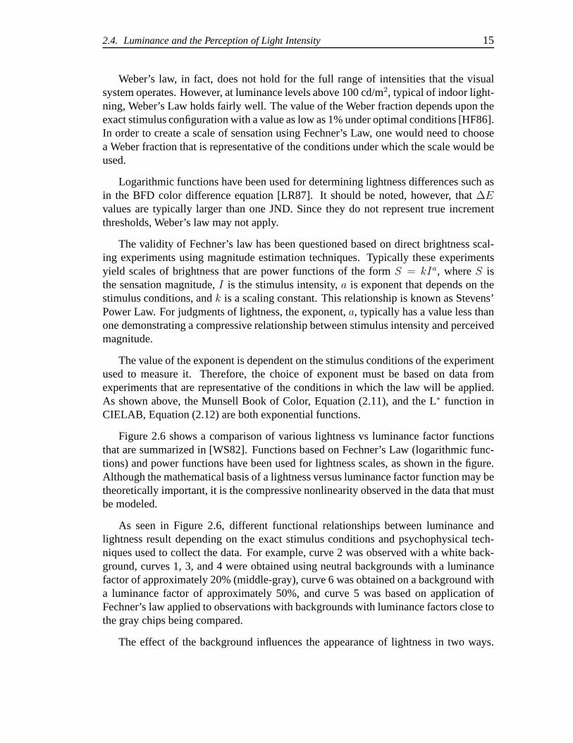
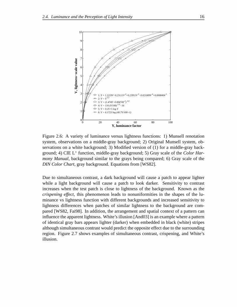
Figure 2.6 shows a comparison of various lightness vs luminance factor functionsthat are summarized in [WS82]. Functions based on Fechner’sLaw (logarithmic func-tions) and power functions have been used for lightness scales, as shown in the figure.Although the mathematical basis of a lightness versus luminance factor function may betheoretically important, it is the compressive nonlinearity observed in the data that mustbe modeled.
As seen in Figure 2.6, different functional relationships between luminance andlightness result depending on the exact stimulus conditions and psychophysical tech-niques used to collect the data. For example, curve 2 was observed with a white back-ground, curves 1, 3, and 4 were obtained using neutral backgrounds with a luminancefactor of approximately 20% (middle-gray), curve 6 was obtained on a background witha luminance factor of approximately 50%, and curve 5 was based on application ofFechner’s law applied to observations with backgrounds with luminance factors close tothe gray chips being compared.
The effect of the background influences the appearance of lightness in two ways.
2.4. Luminance and the Perception of Light Intensity 16
0 20 40 60 80 1000
1
2
3
4
5
6
7
8
9
10
Y, luminance factor
V, l
ight
ness
−sc
ale
valu
e
1: Y = 1.2219V−0.23111V 2+0.23951V 3−0.021009V 4+0.0008404 5 2: V = Y 1/2
3: V = (1.474Y−0.00474Y 2) 1/2
4: V = 116 (Y/100) 1/3−165: V = 0.25+5 log Y
6: V = 6.1723 log (40.7Y/100+1)
Figure 2.6: A variety of luminance versus lightness functions: 1) Munsell renotationsystem, observations on a middle-gray background; 2) Original Munsell system, ob-servations on a white background; 3) Modified version of (1) for a middle-gray back-ground; 4) CIE L∗ function, middle-gray background; 5) Gray scale of theColor Har-mony Manual, background similar to the grays being compared; 6) Gray scale of theDIN Color Chart, gray background. Equations from [WS82].
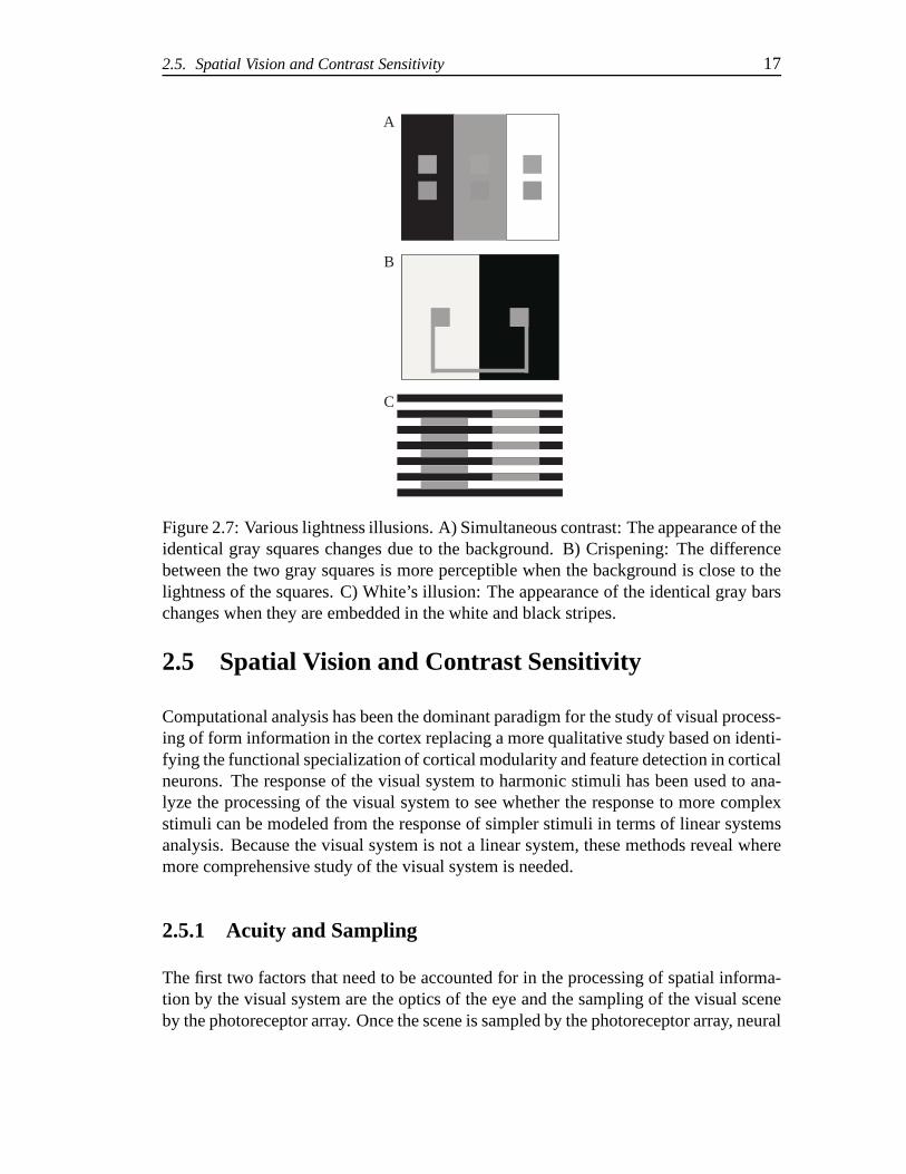
Due to simultaneous contrast, a dark background will cause apatch to appear lighterwhile a light background will cause a patch to look darker. Sensitivity to contrastincreases when the test patch is close to lightness of the background. Known as thecrispening effect, this phenomenon leads to nonuniformities in the shapes of the lu-minance vs lightness function with different backgrounds and increased sensitivity tolightness differences when patches of similar lightness tothe background are com-pared [WS82, Fai98]. In addition, the arrangement and spatial context of a pattern caninfluence the apparent lightness. White’s illusion [And03]is an example where a patternof identical gray bars appears lighter (darker) when embedded in black (white) stripesalthough simultaneous contrast would predict the oppositeeffect due to the surroundingregion. Figure 2.7 shows examples of simultaneous contrast, crispening, and White’sillusion.
2.5. Spatial Vision and Contrast Sensitivity 17
A
B
C
Figure 2.7: Various lightness illusions. A) Simultaneous contrast: The appearance of theidentical gray squares changes due to the background. B) Crispening: The differencebetween the two gray squares is more perceptible when the background is close to thelightness of the squares. C) White’s illusion: The appearance of the identical gray barschanges when they are embedded in the white and black stripes.
2.5 Spatial Vision and Contrast Sensitivity
Computational analysis has been the dominant paradigm for the study of visual process-ing of form information in the cortex replacing a more qualitative study based on identi-fying the functional specialization of cortical modularity and feature detection in corticalneurons. The response of the visual system to harmonic stimuli has been used to ana-lyze the processing of the visual system to see whether the response to more complexstimuli can be modeled from the response of simpler stimuli in terms of linear systemsanalysis. Because the visual system is not a linear system, these methods reveal wheremore comprehensive study of the visual system is needed.
2.5.1 Acuity and Sampling
The first two factors that need to be accounted for in the processing of spatial informa-tion by the visual system are the optics of the eye and the sampling of the visual sceneby the photoreceptor array. Once the scene is sampled by the photoreceptor array, neural
2.5. Spatial Vision and Contrast Sensitivity 18
processing determines the visual response to spatial variation.
Attempts to measure the modulation transfer function (MTF)of the eye have reliedon both physical and psychophysical techniques. Campbell and Gubisch [CG66], forexample, measured the linespread function of the eye by measuring the light from abright line stimulus reflected out of the eye and correcting for the double passage of lightthrough the eye for different pupil sizes. MTFs derived fromdouble-pass measurementscorrespond well with psychophysical measurements derivedfrom laser interferometry inwhich the MTF is estimated from the ratio of contrast sensitivity to conventional gratingsand interference fringes that are not blurred by the optics of the eye [WBMN94]. TheMTF of the eye demonstrates that for 2 mm pupils, the modulation of the signal falls offvery rapidly and is approximately 1% at about 60 cpd. For larger pupils, 4-6 mm, themodulation falls to 1% at approximately 120 cpd [PW03].
In the fovea the cone photoreceptors are packed tightly in a triangular arrangementwith a mean center-to-center spacing of 32 arc min [Wil88]. This corresponds to a sam-pling rate of approximately 120 samples per degree or a Nyquist frequency of around60 cpd. Because the optics of the eye sufficiently degrade theimage above 60 cpd weare spared the effects of spatial aliasing in normal foveal vision. The S-cone packing inthe retina is much more sparse than the M- and L-cone packing so that its Nyquist limitis approximately 10 cpd [PW03].
Visual spatial acuity is therefore considered to be approximately 60 cpd althoughunder special conditions, for example, peripheral vision,large pupil sizes, and laserinterferometry, higher spatial frequencies can be either directly resolved or seen via theeffects of aliasing. This would appear to set a useful limit for the design of displays,for example. However, in addition to the ability of the visual system to detect spatialvariation, there also exists the ability to detect spatial alignment known as Vernier acuityor hyperacuity. In these tasks, observers are able to judge whether two stimuli (dots orline segments) separated by a small gap are misaligned with offsets as small as 2-5 arcsec, which is less than one-fifth the width of a cone [WM77]. Itis hypothesized that itis the blurring of the optics of eye that contributes to this effect by distributing the lightover a number of receptors. By comparing the distributions of the responses to the twostimuli, the visual system can localize the position of the stimuli at a resolution finerthan the receptor spacing [Wan95, DD90].
2.5.2 Contrast Sensitivity
It can be argued that the visual system evolved to discriminate and identify objects inthe world. The requirements for this task are different fromthose needed if the purposeof the visual system was meant to measure and to record the variation of light intensityin the visual field. In this regard, characterization of the visual system’s response tovariations in contrast as a function of spatial frequency isstudied using harmonic stimuli.
2.5. Spatial Vision and Contrast Sensitivity 19
0.1 1 10 1001
10
100
Spatial frequency (cycles/degree)
Con
tras
t sen
sitiv
ity
0.01 cd/m2
0.1 cd/m2
1 cd/m2
10 cd/m2
100 cd/m2
1000 cd/m2
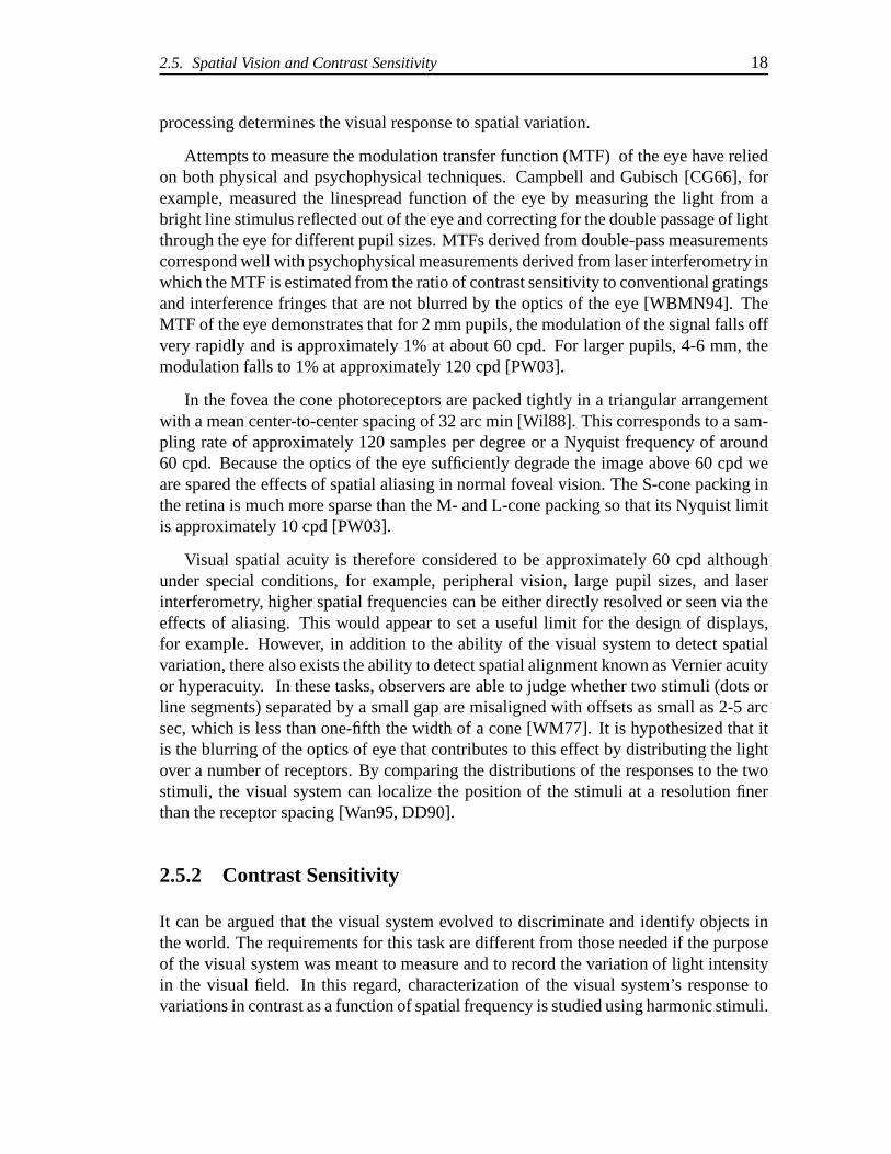
Figure 2.8: Contrast sensitivity function for different mean luminance levels. The curveswere generated using the empirical model of the achromatic CSF in [Bar04].
The contrast sensitivity function (CSF) plots the sensitivity of the visual system tosinusoids of varying spatial frequency.
Figure 2.8 shows the contrast sensitivity of the visual system based on Barten’s em-pirical model [Bar99, Bar04]. The contrast sensitivity is aplot of the reciprocal of thethreshold (ordinate) contrast needed to detect sinusoidalgratings of different spatial fre-quency (abscissa) in cycles per degree of visual angle. Contrast is usually given usingMichelson contrast:(Lmax −Lmin)/(Lmax + Lmin), whereLmax andLmin are the peakand trough luminance of the grating, respectively. Typically plotted on log-log coordi-nates, the CSF reveals the limits of detecting variation in intensity as a function of size.Each curve in Figure 2.8 shows the change in contrast sensitivity for sinusoidal grat-ings modulated around mean luminance levels ranging from 0.01 cd/m2 to 1000 cd/m2.As the mean luminance increases to photopic levels the CSF takes on its characteristicband-pass shape. As luminance increases, the high frequency cut-off, indicating spatialacuity, increases. At scotopic light levels, reduced acuity is due to the increased spatialpooling in the rod pathway which increases absolute sensitivity to light.
As the mean luminance level increases the contrast sensitivity to lower spatial fre-quencies increases and then remains constant. Where these curves converge and overlap,we see that the threshold contrast is constant despite the change in mean luminance. Thisis where Weber’s law holds. At higher spatial frequencies, Weber’s Law breaks down.
The exact shape of the CSF depends on many parametric factorsso that there is no
2.5. Spatial Vision and Contrast Sensitivity 20
one canonical CSF curve [Gra89]. Mean luminance, spatial position on the retina, spa-tial extent (size), orientation, temporal frequency, individual differences, and pathologyare all factors that influence the CSF. (See [Gra89] for a detailed bibliography of studiesrelated to parametric differences.)
Sensitivity is greatest at the fovea and tends to fall off linearly (in terms of log sen-sitivity) with distance from the fovea for each spatial frequency. This fall off is fasterfor higher spatial frequencies so that the CSF becomes more low-pass in the peripheralretina. As the spatial extent (the number of periods) in the stimulus increases, there isan increase in sensitivity up to a point at which sensitivityremains constant. The changein sensitivity with spatial extent changes as the distance from the fovea increases so thatthe most effective stimuli in the periphery are larger than in the fovea. Theoblique effectis the term applied to the reduction in contrast sensitivityto obliquely oriented gratingscompared to horizontally and vertically ones. This reduction in sensitivity (a factor of 2or 3) occurs at high spatial frequencies.
2.5.3 Multiple Spatial Frequency Channels
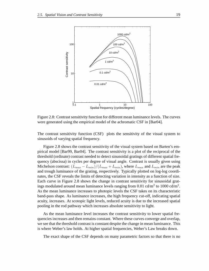
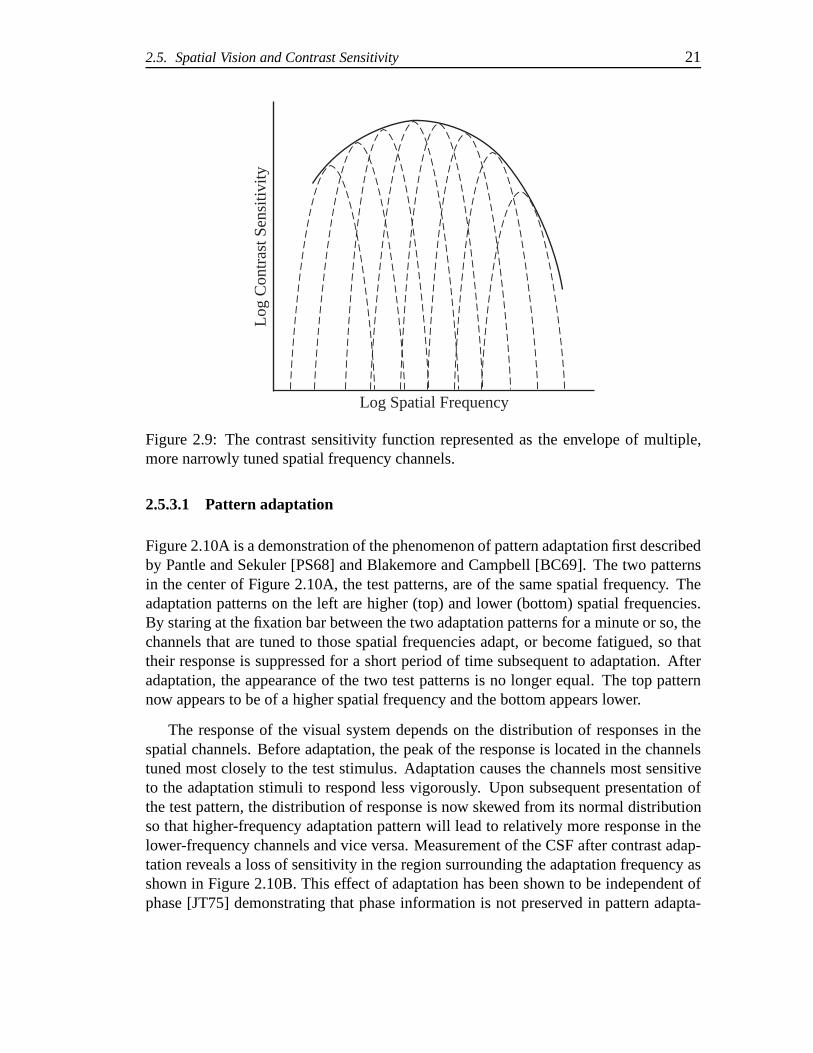
Psychophysical, physiological, and anatomical evidence suggest that the CSF repre-sents the envelope of the sensitivity of many more narrowly tuned channels as shownin Figure 2.9. The idea is that the visual system analyzes thevisual scene in terms ofmultiple channels each sensitive to a narrow range of spatial frequencies. In addition tochannels sensitive to narrow bands of spatial frequency, the scene is also decomposedinto channels sensitive to narrow bands of orientation. This concept of multiresolutionrepresentations forms the basis of many models of spatial vision and pattern sensitivity(see [Wan95, DD90]).
The receptive fields of neurons in the visual cortex are size specific and there-fore show tuning functions that correspond with multiresolution theory and may be thephysiological underpinnings of the psychophysical phenomena described below. Phys-iological evidence points to a continuous distribution of peak frequencies in corticalcells [DD90] although multiresolution models have been built using a discrete numberof spatial channels and orientations (e.g., Wilson and Regan [WR84] suggested a modelwith six spatial channels at eight orientations). Studies have shown that six channelsseem to model psychophysical data well without ruling out a larger number [WLM+90].Both physiological and psychophysical evidence indicate that the bandwidths of the un-derlying channels are broader for lower frequency channelsand become narrower athigher frequencies as plotted on a logarithmic scale of spatial frequency. On a linearscale, however, the low-frequency channels have a much narrower bandwidth than thehigh-frequency channels.
2.5. Spatial Vision and Contrast Sensitivity 21
Log Spatial Frequency
Log
Con
tras
t Sen
sitiv
ity
Figure 2.9: The contrast sensitivity function representedas the envelope of multiple,more narrowly tuned spatial frequency channels.
2.5.3.1 Pattern adaptation
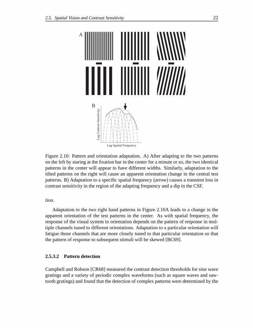
Figure 2.10A is a demonstration of the phenomenon of patternadaptation first describedby Pantle and Sekuler [PS68] and Blakemore and Campbell [BC69]. The two patternsin the center of Figure 2.10A, the test patterns, are of the same spatial frequency. Theadaptation patterns on the left are higher (top) and lower (bottom) spatial frequencies.By staring at the fixation bar between the two adaptation patterns for a minute or so, thechannels that are tuned to those spatial frequencies adapt,or become fatigued, so thattheir response is suppressed for a short period of time subsequent to adaptation. Afteradaptation, the appearance of the two test patterns is no longer equal. The top patternnow appears to be of a higher spatial frequency and the bottomappears lower.
The response of the visual system depends on the distribution of responses in thespatial channels. Before adaptation, the peak of the response is located in the channelstuned most closely to the test stimulus. Adaptation causes the channels most sensitiveto the adaptation stimuli to respond less vigorously. Upon subsequent presentation ofthe test pattern, the distribution of response is now skewedfrom its normal distributionso that higher-frequency adaptation pattern will lead to relatively more response in thelower-frequency channels and vice versa. Measurement of the CSF after contrast adap-tation reveals a loss of sensitivity in the region surrounding the adaptation frequency asshown in Figure 2.10B. This effect of adaptation has been shown to be independent ofphase [JT75] demonstrating that phase information is not preserved in pattern adapta-
2.5. Spatial Vision and Contrast Sensitivity 22
A
Log Spatial Frequency
Log
Con
tras
t Sen
sitiv
ity
B
Figure 2.10: Pattern and orientation adaptation. A) After adapting to the two patternson the left by staring at the fixation bar in the center for a minute or so, the two identicalpatterns in the center will appear to have different widths.Similarly, adaptation to thetilted patterns on the right will cause an apparent orientation change in the central testpatterns. B) Adaptation to a specific spatial frequency (arrow) causes a transient loss incontrast sensitivity in the region of the adapting frequency and a dip in the CSF.
tion.
Adaptation to the two right hand patterns in Figure 2.10A leads to a change in theapparent orientation of the test patterns in the center. As with spatial frequency, theresponse of the visual system to orientation depends on the pattern of response in mul-tiple channels tuned to different orientations. Adaptation to a particular orientation willfatigue those channels that are more closely tuned to that particular orientation so thatthe pattern of response to subsequent stimuli will be skewed[BC69].
2.5.3.2 Pattern detection
Campbell and Robson [CR68] measured the contrast detectionthresholds for sine wavegratings and a variety of periodic complex waveforms (such as square waves and saw-tooth gratings) and found that the detection of complex patterns were determined by the
2.5. Spatial Vision and Contrast Sensitivity 23
contrast of the fundamental component rather than the contrast of the overall pattern.In addition, they observed that the ability to distinguish asquare wave pattern from asinusoid occurred when the third harmonic of the square wavereached its own thresholdcontrast.
Graham and Nachmias [GN71] measured the detection thresholds for gratings com-posed of two frequency components,f and3f , as a function of the relative phase ofthe two gratings. When these two components are added in phase so that their peakscoincide, the overall contrast is higher than when they are combined so that their peakssubtract. However, the thresholds for detecting the gratings were the same regardlessof phase. These results support a spatial frequency analysis of the visual stimulus asopposed to detection based on the luminance profile.
2.5.3.3 Masking and facilitation
The experiments on pattern adaptation and detection dealt with the detection and inter-action of gratings at their contrast threshold levels. The effect of suprathreshold patternson grating detection is more complicated. In these cases a superimposed grating caneither hinder the detection (masking) of a test grating or itcan lead to a lower detectionthreshold (facilitation), depending on the properties of the two gratings. The influenceof the mask on the detectability of the test depends on the spatial frequency, orientation,and phase of the mask relative to the test. This interaction increases as the mask andtarget become more similar. For similar tests and masks, facilitation is seen at low maskcontrasts and as the contrast increases the test is masked.
In the typical experimental paradigm a grating (or a Gabor pattern) of a fixed contrastcalled the “pedestal” or “masking grating” is presented along with a “test” or “signal”grating (or Gabor). The threshold contrast at which the testcan be detected (or discrim-inated in a forced-choice) is measured as a function of the contrast of the mask. Theresulting plot of contrast threshold versus the masking contrast is sometimes referred toas the threshold versus contrast, or TvC, function.
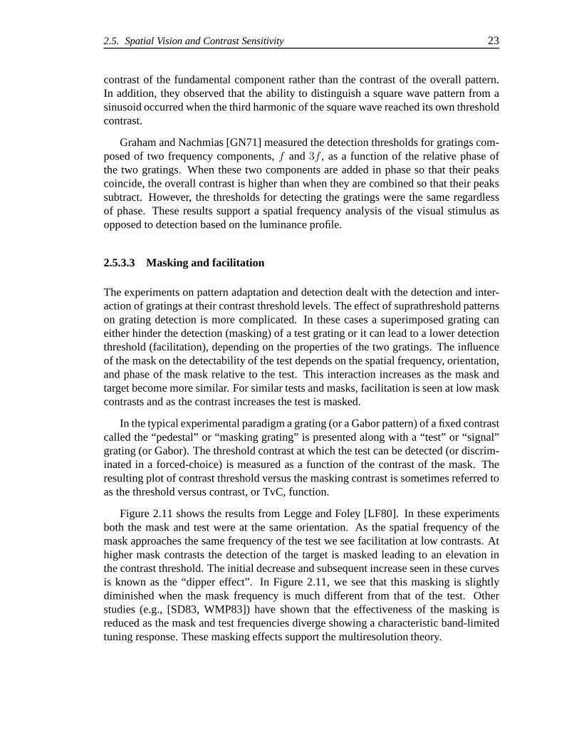
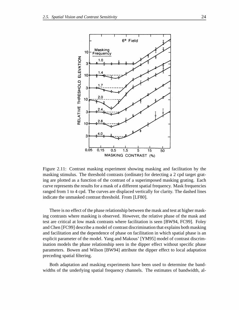
Figure 2.11 shows the results from Legge and Foley [LF80]. Inthese experimentsboth the mask and test were at the same orientation. As the spatial frequency of themask approaches the same frequency of the test we see facilitation at low contrasts. Athigher mask contrasts the detection of the target is masked leading to an elevation inthe contrast threshold. The initial decrease and subsequent increase seen in these curvesis known as the “dipper effect”. In Figure 2.11, we see that this masking is slightlydiminished when the mask frequency is much different from that of the test. Otherstudies (e.g., [SD83, WMP83]) have shown that the effectiveness of the masking isreduced as the mask and test frequencies diverge showing a characteristic band-limitedtuning response. These masking effects support the multiresolution theory.
2.5. Spatial Vision and Contrast Sensitivity 24
Figure 2.11: Contrast masking experiment showing masking and facilitation by themasking stimulus. The threshold contrasts (ordinate) for detecting a 2 cpd target grat-ing are plotted as a function of the contrast of a superimposed masking grating. Eachcurve represents the results for a mask of a different spatial frequency. Mask frequenciesranged from 1 to 4 cpd. The curves are displaced vertically for clarity. The dashed linesindicate the unmasked contrast threshold. From [LF80].
There is no effect of the phase relationship between the maskand test at higher mask-ing contrasts where masking is observed. However, the relative phase of the mask andtest are critical at low mask contrasts where facilitation is seen [BW94, FC99]. Foleyand Chen [FC99] describe a model of contrast discriminationthat explains both maskingand facilitation and the dependence of phase on facilitation in which spatial phase is anexplicit parameter of the model. Yang and Makous’ [YM95] model of contrast discrim-ination models the phase relationship seen in the dipper effect without specific phaseparameters. Bowen and Wilson [BW94] attribute the dipper effect to local adaptationpreceding spatial filtering.
Both adaptation and masking experiments have been used to determine the band-widths of the underlying spatial frequency channels. The estimates of bandwidth, al-
2.5. Spatial Vision and Contrast Sensitivity 25
though variable, correspond to the bandwidths of cells in the primary visual cortex ofanimals studied using physiological techniques [DD90, WLM+90].
Experiments studying the effect of orientation of the mask on target detection haveshown that as the orientation of the mask approaches that of the target, the thresholdcontrast for detecting the target increases. Phillips and Wilson [PW84], for example,measured the threshold elevation caused by masking for various spatial frequencies andmasking contrasts. Their estimates of the orientation bandwidths show a gradual de-crease in bandwidth of about±30◦ at 0.5 cpd to±15◦ at 11.3 cpd which agrees well withphysiological results from macaque striate cortex. No differences were found for testsoriented at0◦ and45◦ indicating that the oblique effect is not due to differencesin band-width at these two orientations but rather is more likely dueto a predominance of cellswith orientation specificity to the horizontal and vertical[PW84]. The same relation-ships found between the spatial and orientation tuning of visual mechanism elucidatedusing the psychophysical masking paradigm agree with thoserevealed in recordingsfrom cells in the macaque primary cortex [WLM+90].
2.5.3.4 Nonindependence in spatial frequency and orientation
The multiresolution representation theory postulates independence among the variousspatial frequency and orientation channels that are analyzing the visual scene. Modelsof spatial contrast discrimination are typically based on the analysis of the stimulusthrough independent spatial frequency channels followed by a decision stage in whichthe outputs from these channels are compared (e.g., [FC99, WR84]).
However, there is considerable evidence of nonlinear interactions between separatespatial frequency and orientation channels that challengea strong form of the multires-olution theory (see [Wan95]). Both physiologically and psychophysically, there is evi-dence of interactions between channels that are far apart intheir tuning characteristics.Figure 2.12 shows two perceptual illustrations of nonlinear interaction for spatial fre-quency (Figure 2.12A) and orientation (Figure 2.12B).
Figure 2.12A shows a grating of frequencyf , top, and a grating that is the sum ofgratings of4f , 5f , and6f . The appearance of the complex grating has a periodicity offrequencyf although there is no component at this frequency. Even though the earlycortical mechanisms tuned tof are not responding to the complex grating, the higherfrequency mechanisms tuned to the region of5f somehow produce signals that fill inthe “missing fundamental” during later visual processing (see [DD90]).
Figure 2.12B shows the grating produced by the sum of two gratings at±67.5◦ fromthe vertical. Although there is no grating components in thehorizontal or vertical direc-tion, there is the appearance of such stripes. Derrington and Henning [DH89] performeda masking experiment in which individual grating at orientations of±67.5◦ did not mask
2.5. Spatial Vision and Contrast Sensitivity 26
Figure 2.12: (A) The top grating has a spatial frequency off . A perceived periodicityof f is seen in the complex grating on the bottom that is the sum of the frequencies of4f , 5f , and6f . Redrawn from [DD90]. (B) The sum of two gratings at±67.5◦ has nohorizontal or vertical components yet these orientations are perceived.
the detection of a vertical grating of the same spatial frequency but the mixture of thetwo gratings produced substantial masking. De Valois [DD90] presents further examplesof interactions between spatial frequency channels from adaptation experiments, phys-iological recordings, and anatomical studies in animals. These studies point to mutualinhibition among spatial frequency and orientation selective channels.
2.5.3.5 Chromatic contrast sensitivity
Sensitivity to spatial variation for color has also been studied using harmonic stimuli.Mullen [Mul85] measured contrast sensitivity to red-greenand blue-yellow gratingsusing counterphase monochromatic stimuli for the chromatic stimuli. The optics of theeye produce chromatic aberrations and magnification differences between the chromaticgratings. These artifacts were controlled by introducing lenses to independently focuseach grating and scaling the size of the gratings. In addition, the relative luminances ofthe gratings were matched at the different spatial frequencies using flicker photometry.
2.5. Spatial Vision and Contrast Sensitivity 27
Figure 2.13: Contrast sensitivity functions of the achromatic luminance channel andthe red-green, and blue yellow opponent chromatic channelsfrom [Mul85]. Solid linesindicate data from one subject. Dashed lines are extrapolated from the measured data toshow the high-frequency acuity limit for the three channelsin this experiment. Redrawnfrom Mullen [Mul85].
The wavelengths for the chromatic gratings were chosen to isolate the two chromatic-opponent mechanisms.
Figure 2.13 shows the resulting luminance and isolumant red-green and blue-yellowCSFs redrawn from one observer in Mullen. The chromatic CSFsare characterized by alow-pass shape and have high frequency cut-offs at much lower spatial frequencies thanthe luminance CSF. The acuity of the blue-yellow mechanism is limited by the sparsedistribution of S-cones in the retinal mosaic, however the lower acuity in the red-greenmechanism is not limited by retinal sampling and is therefore imposed by subsequentneural processing [Mul85, SWB93b].
Sekiguchi et al. [SWB93b, SWB93a] used laser interferometry to eliminate chro-matic aberration with drifting chromatic gratings moving in opposite directions to si-multaneously measure the chromatic and achromatic CSFs. They found a close matchbetween the two chromatic mechanisms and slightly higher sensitivity than Mullens’sresults.
Poirson and Wandell [PW95] used an asymmetric color-matching task to explorethe relationship between pattern vision (spatial frequency) and color appearance. In thistask, square-wave gratings of various spatial frequenciescomposed of pairs of comple-mentary colors (colors whose additive mixture is neutral inappearance) were presentedto observers. The observers’ task was to match the color of a 2-degree square patch tothe colors of the individual bars of the square-wave grating. They found that the colorappearance of the bars depended on the spatial frequency of the pattern. Using a pattern-
2.5. Spatial Vision and Contrast Sensitivity 28
color separable model, Poirson and Wandell derived the spectral sensitivities and spatialcontrast sensitivities of the three mechanisms that mediated the color appearance judg-ments. These mechanisms showed a striking resemblance to the luminance and twochromatic-opponent channels identified psychophysicallyand physiologically.
One outcome of the difference in the spatial response between the chromatic andluminance channels is that the sharpness of an image is judged based on the sharpnessof the luminance information in the image since the visual system is incapable of re-solving high-frequency chromatic information. This has been taken advantage of in thecompression and transmission of color images since the highspatial frequency chro-matic information in an image can be removed without a loss inperceived image quality(e.g., [MF85]). The perceptual salience of many geometric visual illusions is severelydiminished or eliminated when they are reproduced using isoluminant patterns due tothis loss of high spatial frequency information. The minimally distinct border methodfor determining luminance matches is also related to the reduced spatial accuity of thechromatic mechanisms.
2.5.3.6 Suprathreshold contrast sensitivity
The discussion so far has focused on threshold measurementsof contrast. Our sensitivityto contrast at threshold is very dependent on spatial frequency and has been studiedin-depth to understand the limits of visual perception. Therelationship between theperception of contrast and spatial frequency at levels above threshold will be brieflydiscussed here. It should be noted that there is increasing evidence that the effects seenat threshold are qualitatively different from those at suprathreshold levels so that modelsof detection and discrimination may not be applicable (e.g., [FBM03]).
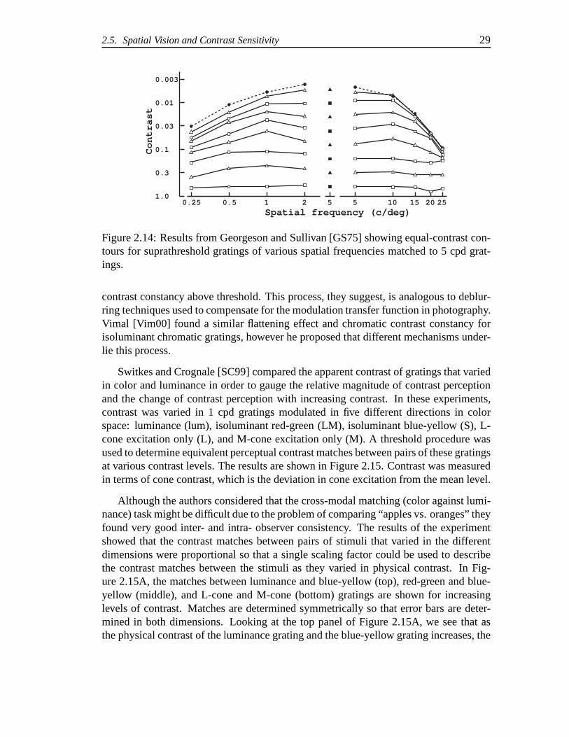
Figure 2.14 presents data for one subject redrawn from Georgeson and Sullivan[GS75] showing the results from a suprathreshold contrast matching experiment. Inthis experiment observers made apparent contrast matches between a standard 5 cpdgrating and test gratings that varied from 0.25 to 25 cpd. Theuppermost contour reflectsthe CSF at threshold. As the contrast of the gratings increased above threshold lev-els, the results showed that the apparent contrast matched when the physical contrastswere equal. This flattening of the equal-contrast contours in Figure 2.14 is more rapidat higher spatial frequencies. The flattening of the contours was termed “contrast con-stancy”. Subjects also made contrast matches using single lines and band-pass filteredimages. Again it was shown that the apparent contrast matched the physical contrastwhen the stimuli were above threshold. Further experimentsdemonstrated that theseresults were largely independent of mean luminance level and position on the retina.
Georgeson and Sullivan suggest that an active process is correcting the neural andoptical blurring seen at threshold for high spatial frequencies. They hypothesize that thevarious spatial frequency channels adjust their gain independently in order to achieve
2.5. Spatial Vision and Contrast Sensitivity 29
25
Spatial frequency (c/deg)
Contrast
0.003
0.01
0.03
0.1
0.3
1.00.25 0.5 1 2 5 5 10 15 20
Figure 2.14: Results from Georgeson and Sullivan [GS75] showing equal-contrast con-tours for suprathreshold gratings of various spatial frequencies matched to 5 cpd grat-ings.
contrast constancy above threshold. This process, they suggest, is analogous to deblur-ring techniques used to compensate for the modulation transfer function in photography.Vimal [Vim00] found a similar flattening effect and chromatic contrast constancy forisoluminant chromatic gratings, however he proposed that different mechanisms under-lie this process.
Switkes and Crognale [SC99] compared the apparent contrastof gratings that variedin color and luminance in order to gauge the relative magnitude of contrast perceptionand the change of contrast perception with increasing contrast. In these experiments,contrast was varied in 1 cpd gratings modulated in five different directions in colorspace: luminance (lum), isoluminant red-green (LM), isoluminant blue-yellow (S), L-cone excitation only (L), and M-cone excitation only (M). A threshold procedure wasused to determine equivalent perceptual contrast matches between pairs of these gratingsat various contrast levels. The results are shown in Figure 2.15. Contrast was measuredin terms of cone contrast, which is the deviation in cone excitation from the mean level.
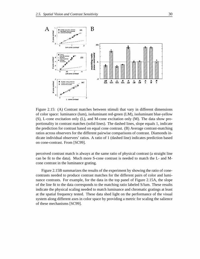
Although the authors considered that the cross-modal matching (color against lumi-nance) task might be difficult due to the problem of comparing“apples vs. oranges” theyfound very good inter- and intra- observer consistency. Theresults of the experimentshowed that the contrast matches between pairs of stimuli that varied in the differentdimensions were proportional so that a single scaling factor could be used to describethe contrast matches between the stimuli as they varied in physical contrast. In Fig-ure 2.15A, the matches between luminance and blue-yellow (top), red-green and blue-yellow (middle), and L-cone and M-cone (bottom) gratings are shown for increasinglevels of contrast. Matches are determined symmetrically so that error bars are deter-mined in both dimensions. Looking at the top panel of Figure 2.15A, we see that asthe physical contrast of the luminance grating and the blue-yellow grating increases, the
2.5. Spatial Vision and Contrast Sensitivity 30
Figure 2.15: (A) Contrast matches between stimuli that varyin different dimensionsof color space: luminance (lum), isoluminant red-green (LM), isoluminant blue-yellow(S), L-cone excitation only (L), and M-cone excitation only(M). The data show pro-portionality in contrast matches (solid lines). The dashedlines, slope equals 1, indicatethe prediction for contrast based on equal cone contrast. (B) Average contrast-matchingratios across observers for the different pairwise comparisons of contrast. Diamonds in-dicate individual observers’ ratios. A ratio of 1 (dashed line) indicates prediction basedon cone-contrast. From [SC99].
perceived contrast match is always at the same ratio of physical contrast (a straight linecan be fit to the data). Much more S-cone contrast is needed to match the L- and M-cone contrast in the luminance grating.
Figure 2.15B summarizes the results of the experiment by showing the ratio of cone-contrasts needed to produce contrast matches for the different pairs of color and lumi-nance contrasts. For example, for the data in the top panel ofFigure 2.15A, the slopeof the line fit to the data corresponds to the matching ratio labeled S/lum. These resultsindicate the physical scaling needed to match luminance andchromatic gratings at leastat the spatial frequency tested. These data shed light on theperformance of the visualsystem along different axes in color space by providing a metric for scaling the salienceof these mechanisms [SC99].
2.5. Spatial Vision and Contrast Sensitivity 31
2.5.3.7 Image compression and image difference
Despite the fact that studies of the ability of the human visual system to detect anddiscriminate patterns do not give a complete understandingof how the visual systemworks to produce our final representation of the world, this information on perceptuallimits can have practical use in imaging applications. For image compression, we canuse this information to help guide the development of perceptually lossless encodingschemes. Similarly, we can use this information to eliminate information from imageryto which the visual system is insensitive in order to computeimage differences based onwhat is visible in the scene.
In his book,Foundations of Vision, Wandell [Wan95] introduces the concepts of thediscrete cosine transformation in JPEG image compression,image compression usingLaplacian pyramids, and wavelet compression. He points outthe similarities betweenthese algorithms and the multiresolution representation theory of pattern vision. Per-ceptually lossless image compression is possible because of the ability to quantize highspatial frequency information in the transformed image. Glenn [Gle93] enumerates andquantifies how the visual effects based on thresholds, whichhave been described in parthere, such as the luminance and chromatic CSFs, pattern masking, the oblique effect,and temporal sensitivity (see below) can contribute to perceptually lossless compres-sion. Zeng et al. [ZDL02] summarize the “visual optimization tools” based on spatialfrequency sensitivity, color sensitivity, and visual masking that are used in JPEG 2000in order to optimize perceptually lossless compression.
It was pointed out above that the reduced resolution of the chromatic channels hadbeen taken advantage of in image compression and transmission. This difference inthe processing of chromatic and achromatic vision has been used for describing imagedifferences in Zhang and Wandell’s extension of CIELAB for digital image reproduc-tion called S-CIELAB for Spatial-CIELAB (Zhang and Wandell[ZW96, ZW88]). Thismethod is intended to compute the visible color difference for determining errors incolor image reproduction.
In this procedure, an original color image and a reproduction are each convertedinto three bands corresponding to the luminance and two opponent chromatic channels.From here, each band is convolved with a spatial filter that removes the informationbeyond the limits of contrast visibility. The images are then converted into CIELABcoordinates where pixel-by-pixel color differences can becomputed.
Johnson and Fairchild [JF02, JF03] explored the use of different CSF functions, in-cluding the standard S-CIELAB filters, on their ability to predict image differences.They found that the use of filters that were normalized to maintain the DC componentof the image performed better [JF02]. This also has an effectof boosting the gain forcertain spatial frequencies since the function produces a filter with coefficients greaterthan one when the DC component is fixed at a value of one. In addition, they found that
2.6. Temporal Vision and Motion 32
anisotropic filters (with parameters that predict the oblique effect), such as the one usedin Daly’s Visible Difference Predictor [Dal93], improve the predictions of the image dif-ference model. Johnson and Fairchild [JF02] also applied spatial frequency adaptation,both a generic statistical model based on the1/f approximation of spatial frequencycontent in natural scenes and an image dependent model, in their image difference pre-dictor and found improvement. This adaptation tends to shift the peak of the CSF tohigher frequencies.
2.6 Temporal Vision and Motion
The sensitivity of the visual system to change over time and the perception of objectmotion are often linked together because the stimuli for motion produce temporal vari-ations in light intensity falling on the retina. It follows that the perception of motion,at the early stages of visual processing, is driven by the same mechanisms that detectchanges in intensity over time. In this section, the response of the visual system to tem-porally periodic stimuli will be briefly presented, followed by a short discussion of realand apparent motion.
2.6.1 Temporal CSF
Before the application of linear systems theory to the studyof temporal vision, the lit-erature was dominated by studies that examined the temporalsensitivity of the eye interms of the critical flicker frequency (CFF) of periodic waveforms modulated in am-plitude [Wat86]. CFF refers to the temporal frequency (Hz) at which the perceptionof flicker in the stimulus changes to a steady or fused appearance. Two concepts thatemerged from this work are the Ferry-Porter law and the Talbot-Plateau law. The Ferry-Porter law states that CFF rises linearly with the logarithmof the time-average back-ground intensity. The Talbot-Plateau law states that the perceived intensity of a fusedperiodic stimulus is the same as a steady stimulus of the sametime-average intensity.
De Lange [de 54, de 58] introduced the ability to modulate temporal contrast whilekeeping the time-average background constant, which allowed the measurement of CFFand temporal contrast sensitivity at various mean intensities and temporal frequencies.His application of linear systems theory produced a coherent framework for interpretingthe literature on temporal sensitivity [Wat86].
In a typical experiment for the measurement of temporal contrast sensitivity a gratingis modulated temporally in counterphase so that the contrast reverses sinusoidally overtime (see Figure 2.16). The contrast threshold for detecting a pattern is measured as afunction of both the temporal frequency of the modulation and the spatial frequency of
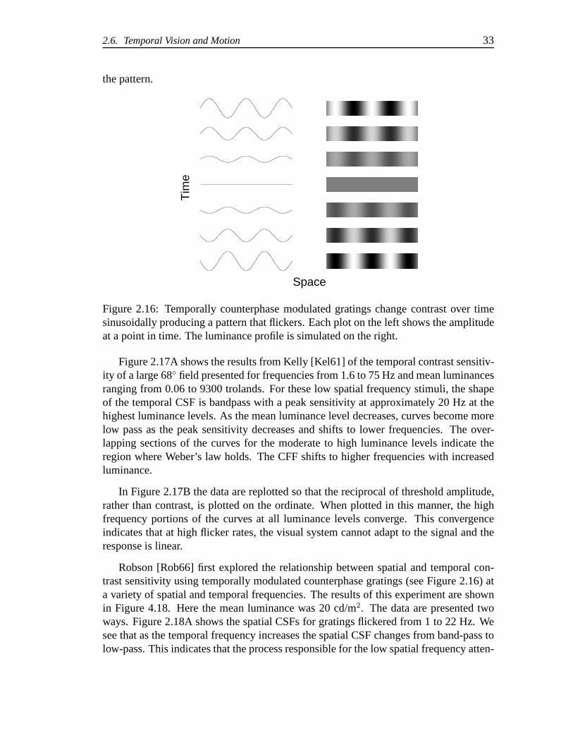
2.6. Temporal Vision and Motion 33
the pattern.
Tim
e
Space
Figure 2.16: Temporally counterphase modulated gratings change contrast over timesinusoidally producing a pattern that flickers. Each plot onthe left shows the amplitudeat a point in time. The luminance profile is simulated on the right.
Figure 2.17A shows the results from Kelly [Kel61] of the temporal contrast sensitiv-ity of a large 68◦ field presented for frequencies from 1.6 to 75 Hz and mean luminancesranging from 0.06 to 9300 trolands. For these low spatial frequency stimuli, the shapeof the temporal CSF is bandpass with a peak sensitivity at approximately 20 Hz at thehighest luminance levels. As the mean luminance level decreases, curves become morelow pass as the peak sensitivity decreases and shifts to lower frequencies. The over-lapping sections of the curves for the moderate to high luminance levels indicate theregion where Weber’s law holds. The CFF shifts to higher frequencies with increasedluminance.
In Figure 2.17B the data are replotted so that the reciprocalof threshold amplitude,rather than contrast, is plotted on the ordinate. When plotted in this manner, the highfrequency portions of the curves at all luminance levels converge. This convergenceindicates that at high flicker rates, the visual system cannot adapt to the signal and theresponse is linear.
Robson [Rob66] first explored the relationship between spatial and temporal con-trast sensitivity using temporally modulated counterphase gratings (see Figure 2.16) ata variety of spatial and temporal frequencies. The results of this experiment are shownin Figure 4.18. Here the mean luminance was 20 cd/m2. The data are presented twoways. Figure 2.18A shows the spatial CSFs for gratings flickered from 1 to 22 Hz. Wesee that as the temporal frequency increases the spatial CSFchanges from band-pass tolow-pass. This indicates that the process responsible for the low spatial frequency atten-
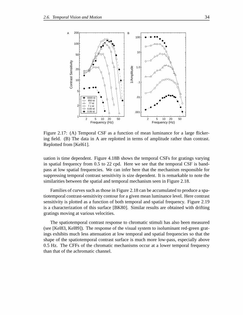
2.6. Temporal Vision and Motion 34
2 5 10 20 501
2
5
10
20
50
100
200
Frequency (Hz)
Con
tras
t Sen
sitiv
ity
9300 td 850 td 77 td 7.1 td0.65 td0.06 td
2 5 10 20 50
.001
.01
.1
1.0
10
100
Frequency (Hz)
1/A
mpl
itude
A B
Figure 2.17: (A) Temporal CSF as a function of mean luminancefor a large flicker-ing field. (B) The data in A are replotted in terms of amplituderather than contrast.Replotted from [Kel61].
uation is time dependent. Figure 4.18B shows the temporal CSFs for gratings varyingin spatial frequency from 0.5 to 22 cpd. Here we see that the temporal CSF is band-pass at low spatial frequencies. We can infer here that the mechanism responsible forsuppressing temporal contrast sensitivity is size dependent. It is remarkable to note thesimilarities between the spatial and temporal mechanism seen in Figure 2.18.
Families of curves such as those in Figure 2.18 can be accumulated to produce a spa-tiotemporal contrast-sensitivity contour for a given meanluminance level. Here contrastsensitivity is plotted as a function of both temporal and spatial frequency. Figure 2.19is a characterization of this surface [BK80]. Similar results are obtained with driftinggratings moving at various velocities.
The spatiotemporal contrast response to chromatic stimulihas also been measured(see [Kel83, Kel89]). The response of the visual system to isoluminant red-green grat-ings exhibits much less attenuation at low temporal and spatial frequencies so that theshape of the spatiotemporal contrast surface is much more low-pass, especially above0.5 Hz. The CFFs of the chromatic mechanisms occur at a lower temporal frequencythan that of the achromatic channel.
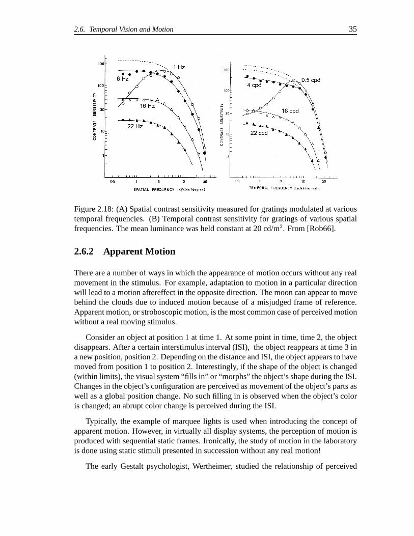
2.6. Temporal Vision and Motion 35
Figure 2.18: (A) Spatial contrast sensitivity measured forgratings modulated at varioustemporal frequencies. (B) Temporal contrast sensitivity for gratings of various spatialfrequencies. The mean luminance was held constant at 20 cd/m2. From [Rob66].
2.6.2 Apparent Motion
There are a number of ways in which the appearance of motion occurs without any realmovement in the stimulus. For example, adaptation to motionin a particular directionwill lead to a motion aftereffect in the opposite direction.The moon can appear to movebehind the clouds due to induced motion because of a misjudged frame of reference.Apparent motion, or stroboscopic motion, is the most commoncase of perceived motionwithout a real moving stimulus.
Consider an object at position 1 at time 1. At some point in time, time 2, the objectdisappears. After a certain interstimulus interval (ISI),the object reappears at time 3 ina new position, position 2. Depending on the distance and ISI, the object appears to havemoved from position 1 to position 2. Interestingly, if the shape of the object is changed(within limits), the visual system “fills in” or “morphs” theobject’s shape during the ISI.Changes in the object’s configuration are perceived as movement of the object’s parts aswell as a global position change. No such filling in is observed when the object’s coloris changed; an abrupt color change is perceived during the ISI.
Typically, the example of marquee lights is used when introducing the concept ofapparent motion. However, in virtually all display systems, the perception of motion isproduced with sequential static frames. Ironically, the study of motion in the laboratoryis done using static stimuli presented in succession without any real motion!
The early Gestalt psychologist, Wertheimer, studied the relationship of perceived
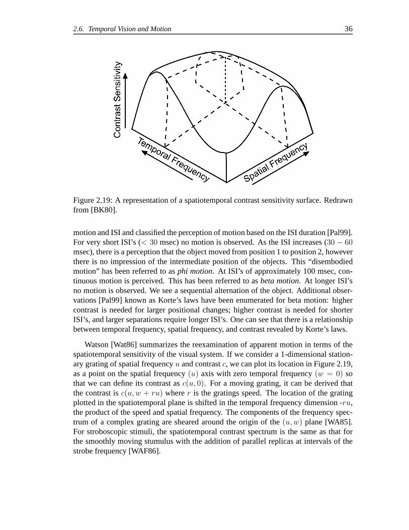
2.6. Temporal Vision and Motion 36
Figure 2.19: A representation of a spatiotemporal contrastsensitivity surface. Redrawnfrom [BK80].
motion and ISI and classified the perception of motion based on the ISI duration [Pal99].For very short ISI’s (< 30 msec) no motion is observed. As the ISI increases (30 − 60msec), there is a perception that the object moved from position 1 to position 2, howeverthere is no impression of the intermediate position of the objects. This “disembodiedmotion” has been referred to asphi motion. At ISI’s of approximately 100 msec, con-tinuous motion is perceived. This has been referred to asbeta motion. At longer ISI’sno motion is observed. We see a sequential alternation of theobject. Additional obser-vations [Pal99] known as Korte’s laws have been enumerated for beta motion: highercontrast is needed for larger positional changes; higher contrast is needed for shorterISI’s, and larger separations require longer ISI’s. One cansee that there is a relationshipbetween temporal frequency, spatial frequency, and contrast revealed by Korte’s laws.
Watson [Wat86] summarizes the reexamination of apparent motion in terms of thespatiotemporal sensitivity of the visual system. If we consider a 1-dimensional station-ary grating of spatial frequencyu and contrastc, we can plot its location in Figure 2.19,as a point on the spatial frequency(u) axis with zero temporal frequency(w = 0) sothat we can define its contrast asc(u, 0). For a moving grating, it can be derived thatthe contrast isc(u, w + ru) wherer is the gratings speed. The location of the gratingplotted in the spatiotemporal plane is shifted in the temporal frequency dimension -ru,the product of the speed and spatial frequency. The components of the frequency spec-trum of a complex grating are sheared around the origin of the(u, w) plane [WA85].For stroboscopic stimuli, the spatiotemporal contrast spectrum is the same as that forthe smoothly moving stumulus with the addition of parallel replicas at intervals of thestrobe frequency [WAF86].
2.7. Visual Modeling 37
For stroboscopic vision to appear smooth and real, Watson etal. [WAF86] predictedthat the contrast of parallel replicas of the stimuli must bebeyond the sensitivity of thevisual system. That is, the temporal and spatial frequency spectra of these replicationsshould be of sufficiently low contrast or beyond the CFF and acuity limits. Psychophysi-cal tests of this prediction were confirmed. These results have implication for the designof motion capture and display systems to reduce the visibility of the aliasing compo-nents.
2.7 Visual Modeling
Visual modeling in one form or another has become an integralpart of the study of thevisual system. Rarely are basic psychophysical and physiological findings not put inthe context of a model of visual processing in order to provide an understanding of thedata in context of what is known about the visual system. Thisis necessary in order toassemble a full picture of the complexity of visual processing given that discoveries aremade in small steps looking at specific aspects of visual function. In addition to the goalof understanding how vision works, what other purposes can visual modeling serve?
One possible goal, machine vision, is to simulate human vision in order to createsystems that can replace humans for certain tasks. Another reason to study human vi-sion is to discover the processing algorithms used by the visual system and apply thesealgorithms in other contexts. Wandell [Wan95] points out that until we fully understandwhy the visual system works the way it does, it is more likely that vision scientists willlearn more from engineers than engineers will learn from vision scientists.
One other goal of modeling visual processing is in order to improve our ability to re-produce the visual world. Imagine a camera that can accurately capture, pixel for pixel,the complete spectral and radiometric information in a scene. Now imagine a device thatcan play it back with complete fidelity (perhaps some virtualreality environment). If wehad such devices, there would be no need to understand visionfrom an application pointof view. However, because we are limited in our ability to capture and display imagery,we need to discover the relevant information that must be captured and how to displayit. Our reproductions are generally presented at a different size, resolution, adaptationlevel, dynamic range and surround environment, to name a few. We must therefore un-derstand how vision processes the original scene information in order to best reproducethe scene.
2.7. Visual Modeling 38
2.7.1 Image and Video Quality Research
There has been significant research applying visual models to video quality and videoquality metrics, often aimed at the creation and optimization of encoding/compression/decoding algorithms such as MPEG-2 and MPEG-4. The static-image visible differ-ences predictor of Daly [Dal93] is one such model used to predict the visibility of arti-facts introduced into still images by JPEG image compression, for example. The Dalymodel was designed to predict the probability of detecting an artifact (i.e., is the artifactabove the visual threshold).
Recently, Fairchild has been developing an image appearance model, iCAM (forimage color appearance model) that has had a different objective with respect to imagequality [FJ02, FJ03]. Instead of focusing on threshold differences in quality, this workhas focused on the prediction of image quality scales (e.g.,scales of sharpness, contrast,graininess) for images with changes well above threshold. The question has not been“can a difference be perceived”, but rather “how large is theperceived difference”. Suchsuprathreshold image differences are a new domain of image quality research based onimage appearance that separate the iCAM model from previousimage quality models.
A similar situation exists in the area of video quality metrics. Metrics have beenpublished to examine the probability of detection of artifacts in video (i.e., thresholdmetrics). Two well-known video image quality models are theSarnoff JND model andthe NASA DVQ model.
The Sarnoff JND model, a proprietary model of human vision [ATI01], is based onthe multi-scale model of spatial vision published by Lubin [Lub93, Lub95] with someextensions for color processing and temporal variation. The Lubin model is similar innature to the Daly model mentioned above in that it is designed to predict the probabilityof detection of artifacts in images. These are threshold changes in images often referredto as just-noticeable differences, or JNDs. The Sarnoff JNDmodel has no mechanismsof chromatic and luminance adaptation, as are included in the iCAM model [FJ02]. Theinput to the Sarnoff model must first be normalized (which canbe considered a veryrudimentary form of adaptation). The temporal aspects of the Sarnoff model are aimed atpredicting the detectability of temporal artifacts. The model only uses two frames (fourfields) in its temporal processing. Thus, it is capable of predicting the perceptibility ofrelatively high frequency temporal variation in the video.It cannot predict the visibilityof low frequency variations that would require an appearance-oriented, rather than JND-oriented model. The Sarnoff model also cannot be used for rendering video, but rather islimited to the prediction of difference-visibility maps ona frame-by-frame basis. Whileit is well accepted in the vision science literature that JNDpredictions are not linearlyrelated to suprathreshold appearance differences, it is certainly possible to use a JNDmodel to try to predict suprathreshold image differences and the Sarnoff JND model hasbeen applied with some success to such data.
2.8. Conclusions 39
A similar model, the DVQ (Digital Video Quality) metric has been published byWatson and colleagues [Wat98, WHM01]. The DVQ metric is similar in concept to theSarnoff JND model, but significantly different in implementation. Its spatial decompo-sition is based on the coefficients of a discrete cosine transformation (DCT) making itamenable to hardware implementation and likely making it particularly good at detect-ing artifacts introduced by DCT-based video compression algorithms. It also has a morerobust temporal filter that should be capable of predicting awider array of temporal ar-tifacts. Like the Sarnoff model, the DVQ metric is aimed at predicting the probabilityof detection of threshold image differences.
2.8 Conclusions
In this chapter we presented a basic outline of some of the psychophysical aspects ofvision focusing on color vision, spatial vision, and temporal vision. At first glance, itmay seem that our knowledge of the visual system based on the rather simple stimuliused in the laboratory may be quite rudimentary when we compare these stimuli to thecomplexity seen in the visual world. However, it is not the case that simple stimuli areused in visual psychophysics because they are easy. Rather,they are chosen in order tobuild up our knowledge of visual perception based on first principles. Before we canunderstand how we see objects, we must understand how the visual system responds topatterns. And before we can fully understand this we must know how the visual systemresponds to intensity. Although the stimuli used in psychophysical experiments mayappear artificial, they are designed to measure specific aspects of visual function.
Notwithstanding, the gains in understanding of visual processing have had success-ful application to practical imaging. In this regard, the use of vision models for imagecompression and image quality has been briefly discussed. Inorder for there to be con-tinued opportunity for the application of vision research and color science to technicalchallenges in video and imagery there must be continued interaction among the basicresearch community and the engineering and technical community in industry. By pro-viding a brief summary of human vision, it is hoped that this chapter will facilitate thisinteraction.
Bibliography
[And03] B. L. Anderson. Perceptual Organization and White’s Illusion. Perception,32(3):269–284, 2003.
[ATI01] ATIS. Iobjective perceptual video quality measurement using a jnd-based full ref-erence technique. Technical Report T1.TR.PP.75-2001, Alliance for Telecommu-nications Industry Solutions Technical Report, 2001.
[Bar99] P. G. J. Barten.Contrast Sensitivity of the Human Eye and Its Effects on ImageQuality. Bellingham, WA: SPIE Press, 1999.
[Bar04] P. G. J. Barten. Formula for the Contrast Sensitivity of the Human Eye. InY. Miyake and D. R. Rasmussen, editors,Image Quality and System Performan-cei, Proceedings of SPIE-IS&T Electronic Imaging, volume 5294, pages 231–238,2004. Y. Miyake and D. R. Rasmussen, eds.
[BC69] C. Blakemore and F. W. Campbell. On the Existence of Neurons in the HumanVisual System Selectively Sensitive to the Orientation andSize of Retinal Images.J. Physiol., 203:237–260, 1969.
[Ber00] R. S. Berns.Billmeyer and Salzman’s Principles of Color Technology. NY: JohnWiley & Sons, Inc., 2000. L. M. Hurvich and D. Jameson, Trans.
[BK80] C. A. Burbeck and D. H. Kelly. Spatiotemporal Characteristics of Visual Mecha-nisms: Excitatory-Inhibitory Model.J. Opt. Soc. Am., 70(9):1121–1126, 1980.
[Boy96] R. M. Boynton. History and Current Status of a Physiologically Based System ofPhotometry and Colorimetry.J. Opt. Soc. Am. A, 13(8):1609–1621, 1996.
[BW94] R. W. Bowen and H. R. Wilson. A Two-Process Analysis ofPattern Masking.Vision Research, 34:645–658, 1994.
[CG66] F. W. Campbell and R. W. Gubisch. Optical Quality of the Human Eye.J. Physiol.,186:558–578, 1966.
[CIE86] CIE No. 15.2. Colorimetry. Commission Internationale de l’Eclairage, Vienna,Austria, 2 edition, 1986.
[CR68] F. W. Campbell and J. G. Robson. Application of Fourier Analysis to the Visibilityof Gratings.J. Physiol., 197:551–566, 1968.
Bibliography 41
[Dal93] S. Daly. The Visible Differences Predictor: An Algorithm for the Assessment ofImage Fidelity. In A. W. Watson, editor,Digital Images and Human Vision, pages179–206. Cambridge, MA: MIT Press, 1993. A. W. Watson, ed.
[DD90] R. L. De Valois and K. K. De Valois.Spatial Vision. NY: Oxford University Press,1990.
[de 54] H. de Lange. Relationship Between Critical Flicker Frequency and a Set of LowFrequency Characteristics of the Eye.J. Opt. Soc. Am., 44:380–389, 1954.
[de 58] H. de Lange. Relationship Between Critical Flicker Frequency and a Set of LowFrequency Characteristics of the Eye.J. Opt. Soc. Am., 48:777–784, 1958.
[DH89] A. M. Derrington and G. B. Henning. Some Observationson the Masking Effectsof Two-Dimensional Stimuli.Vision Research, 28:241–246, 1989.
[Ess03] D. C. Van Essen. Organization of the Visual Areas in Macaque and Human Cere-bral Cortex. In L. M. Chalupa and J. S. Werner, editors,The Visual Sciences, pages507–521. MIT Press, June 2003. L. M. Chalupa and J. S. Werner,eds.
[Fai98] M. D. Fairchild.Color Appearance Models. Reading, MA: Addison-Wesley, 1998.
[FBM03] J. Fiser, P. J. Bex, and W. Makous. Contrast Conservation in Human Vision.VisionResearch, 43(25):2637– 2648, 2003.
[FC99] J. M. Foley and C.-C. Chen. Pattern Detection in the Presence of Maskers that Dif-fer in Spatial Phase and Temporal Offset: Threshold Measurements and a Model.Vision Research, 39:3855–3872, 1999.
[FJ02] M. D. Fairchild and G. M. Johnson. Meet iCAM: A Next-Generation cColor Ap-pearance Model. InProceedings of IS&T/SID 10th Color Imaging Conference,pages 33–38, Scottsdale, AZ, 2002.
[FJ03] M. D. Fairchild and G. M. Johnson. Image Appearance Modeling. In B. R. Ro-gowitz and T. N. Pappas, editors,Human Vision and Electronic Imaging VIII, Pro-ceedings of SPIE-IS&T Electronic Imaging, volume 5007, pages 149–160, 2003.B. R. Rogowitz and T. N. Pappas, eds.
[Gle93] W. E. Glenn. Digital Image Compression Based on Visual Perception. In A. W.Watson, editor,Digital Images and Human Vision, pages 63–72. Cambridge, MA:MIT Press, 1993. A. W. Watson, ed.
[GN71] N. Graham and J. Nachmias. Detection of Grating Patterns Containing Two SpatialFrequencies: A Comparison of Single Channel and Multichannel Models. VisionResearch, 11:251–259, 1971.
[Gra89] N. V. S. Graham.Visual Pattern Analyzers. NY: Oxford University Press, 1989.
[GS75] M. A. Georgeson and G. D. Sullivan. Contrast Constancy: Deblurring in HumanVision by Spatial Frequency Channels.J. Physiol., 252(3):627–656, 1975.
Bibliography 42
[Her64] E. Hering. Outlines of a Theory of the Light Sense. Cambridge, MA: HarvardUniversity Press, 1920/1964. L. M. Hurvich and D. Jameson, Trans.
[HF86] D. C. Hood and M. A. Finkelstein. Sensitivity to Light. In K. R. Boff, L. Kaufman,and J. P. Thoma, editors,Handbook of Perception and Human Performance, Vol. 1:Sensory Processes and Perception, pages (5–1)–(5–66), Vienna, 1963, 1986. NewYork: John Wiley & Sons. K. R. Boff and L. Kaufman and J. P. Thoma, eds.
[JF02] G. M. Johnson and M. D. Fairchild. On Contrast Sensitivity in an Image DifferenceModel. InProceedings of the IS&T PICS Conference, pages 18–23, Portland, OR,2002.
[JF03] G. M. Johnson and M. D. Faichild. Measuring Images: Differences, Quality, andAppearance. In B. R. Rogowitz and T. N. Pappas, editors,Human Vision andElectronic Imaging VIII, Proceedings of SPIE, volume 5007, pages 51–60, 2003.B. R. Rogowitz and T. N. Pappas, eds.
[JT75] R. M. Jones and U. Tulunay-Keesey. Local Retinal Adaptation and Spatial Fre-quency Channels.Vision Research, 15:1239–1244, 1975.
[KB96] P. K. Kaiser and R. M. Boynton.Human Color Vision. Washington, DC: OpticalSociety of America, 2 edition, 1996.
[Kel61] D. H. Kelly. Visual Responses to Time-Dependent Stimuli, I. Amplitude Sensitiv-ity Measurements.J. Opt. Soc. Am., 51(4):422–429, 1961.
[Kel83] D. H. Kelly. Spatiotemporal variation of Chromaticand Achromatic ContrastThresholds.J. Opt. Soc. Am., 73(11):1784–1793, 1983.
[Kel89] D. H. Kelly. Opponent-Color Receptive-Field Profiles determined from Large-Area Psychophysical Measurements.J. Opt. Soc. Am. A, 6(11):1784–1793, 1989.
[KNM84] S. W. Kuffler, J. G. Nicholls, and A. R. Martin.From Neuron to Brain. Sunderland,MA: Sinauer Associates Inc., 2 edition, 1984.
[LCR01] M. R. Luo, G. Cui, and B. Rigg. The Development of the CIE 2000 Colour-Difference Formula: CIEDE2000.Color Researcha nd Application, 26(5):340–350, 2001.
[LF80] G. E. Legge and J. M. Foley. Contrast Masking in Human Vision. J. Opt. Soc. Am.,70(12):1458–1471, 1980.
[LR87] M. R. Luo and B. Rigg. BFD (l:c) Colour-Difference Formula, Part 1 - Develop-ment of the Formula.J. Soc. Dyers. Colour, 103:86–94, 1987.
[Lub93] J. Lubin. The use of psychophysical data and models in the analysis of displaysystem performance. In A. W. Watson, editor,Digital Images and Human Vision,pages 163–178. Cambridge, MA: MIT Press, 1993. A. W. Watson,ed.
Bibliography 43
[Lub95] J. Lubin. A visual discrimination model for imagingsystem design and evaluation.In E. Peli, editor,Vision Models for Target Detection and Recognition, pages 245–283. World Scientific, Singapore, 1995. E. Peli, ed.
[MF85] N. M. Moroney and M. D. Fairchild. Color Space Selection for JPEG Image Com-pression.J. Electronic Imaging, 4(4):373–381, 1985.
[MFH+02] N. Moroney, M. D. Fairchild, R. W. G. Hunt, C. Li, M. R. Luo,and T. Newman.The CIECAM02 Color Appearance Model. InProceedings of IS&T/SID TenthColor Imaging Conference, pages 23–27, Scottsdale, AZ, 2002.
[MM93] W. H. Merigan and J. H. R. Maunsell. How Parallel are the Primate Visual Path-ways.Annual Review of Neuroscience, 16:369–402, 1993.
[Mul85] K. T. Mullen. The Contrast Sensitivity of Human Colour Vision to Red-Green anBlue-Yellow Chromatic Gratings.J. Physiol., 359:381–400, 1985.
[Nic76] D. Nickerson. History of the Munsell Color System.Color Research and Applica-tion, 1:121–130, 1976.
[Pal99] S. E. Palmer.Vision Science: Photons to Phenomenology. Cambridge, MA: MITPress, 1999.
[PS68] A. Pantle and R. W. Sekular. Size-Detection Mechanisms in Human Vision.Sci-ence, 162:1146–1148, 1968.
[PW84] G. C. Phillips and H. R. Wilson. Orientation Bandwidths of Spatial MechanismsMeasured by Masking.J. Opt. Soc. Am. A, 1(2):226–232, 1984.
[PW95] A. B. Poirson and B. A. Wandell. The Appearance of Colored Patterns: Pattern-Color Separability.J. Opt. Soc. Am. A, 12:2458–2471, 1995.
[PW03] O. Packer and D. R. Williams. Light, the Retinal Image, and Photoreceptors. InS. K. Shevell, editor,The Science of Color, pages 41–102. NY: Optical Society ofAmerica, 2003. S. K. Shevell, ed.
[Rob66] J. G. Robson. Spatial and Temporal Contrast-Sensitivity Functions of the VisualSystem.J. Opt. Soc. Am., 56(8):1141–1142, 1966.
[SC99] E. Switkes and M. A. Crognale. Comparison of Color andLuminance Contrast:Apples Versus Oranges?Vision Research, 39(10):1823–1832, 1999.
[SD83] E. Switkes and K. K. DeValois. Luminance and Chromaticity Interactions in Spa-tial Vision. In J. D. Mollon and L. T. Sharpe, editors,Colour Vision, pages 465–470. London: Academic Press, 1983. J. D. Mollon and L. T. Sharpe, eds.
[SS99] A. Stockman and L. T. Sharpe. Cone Spectral Sensitivities and Color Matching.In K. R. Gegenfurtner and L. T. Sharpe, editors,Color Vision, pages 53–88. Cam-bridge University Press, 1999. K. R. Gegenfurtner and L. T. Sharpe, eds.
Bibliography 44
[SW64] C. L. Sanders and G. Wyszecki. Correlate for Brightness in Terms of CIE ColorMatching Data. InCIE Proceedings 15th Session, pages Paper P–63.6. CIE CentralBureau, Paris, 1964.
[SWB93a] N. Sekiguchi, D. R. Williams, and D. H. Brainard. Aberration-Free Measurementsof the Visibility of Isoluminant Gratings.J. Opt. Soc. Am. A, 10(10):2105–2117,1993.
[SWB93b] N. Sekiguchi, D. R. Williams, and D. H. Brainard. Efficiency in Detection of Iso-luminant and Isochromatic Interference Fringes.J. Opt. Soc. Am. A, 10(10):2118–2133, 1993.
[vH11] H. v. Helmholtz.Treatise on Physiological Optics. Rochester, NY: Optical Societyof America, 1866/1911. Translated from 3rd German ed., J. P.Southall, Ed. andTrans.
[Vim00] R. L. P. Vimal. Spatial Color Contrast Matching: Broad-Bandpass Functions andthe Flattening Effect.Vision Research, 40(23):3231–3244, 2000.
[WA85] A. B. Watson and A. J. Ahumada, Jr. Model of Human Visual-Motion Sensing.J.Opt. Soc. Am. A, 2(2):322–342, 1985.
[WAF86] A. B. Watson, A. J. Ahumada, Jr., and J. E. Farrell. Window of Visibility: APsychophysical Theory of Fidelity in Time-Sampled Visual Motion Displays. J.Opt. Soc. Am. A, 3(3):300–307, 1986.
[Wan95] B. A. Wandell.Foundations of Vision. Sunderland, MA: Sinauer Associates, Inc.,1995.
[Wat86] A. B. Watson. Temporal Sensitivity. In K. R. Boff, L.Kaufman, , and J. P.Thoma, editors,Handbook of Perception and Human Performance, Vol. 1: Sen-sory Processes and Perception, pages (6–1)–(6–43). New York: John Wiley &Sons, 1986. K. R. Boff and L. Kaufman and J. P. Thoma, eds.
[Wat98] A. B. Watson. Toward a perceptual video quality metric. In Human Vision andElectronic Imaging III, volume 3299, pages 139–147. SPIE, 1998.
[WBMN94] D. R. Williams, D. H. Brainard, M. J. McMahon, and R.Navarro. Double-Passand Interferometric Measures of the Optical Quality of the Eye. J. Opt. Soc. Am.A, 11(12):3123–3135, 1994.
[WHM01] A. B. Watson, J. Hu, and J. F. McGowan. DVQ: A digital video quality metricbased on human vision.J. Electronic Imaging, 10:20–29, 2001.
[Wil88] D. R. Williams. Topography of the Foveal Cone Mosaicin the Living Human Eye.Vision Research, 28(3):433–454, 1988.
[WLM +90] H. R. Wilson, D. Levi, L. Maffei, J. Rovamo, and R. DeValois. The Perception ofForm: Retina to Striate Cortex. In L. Spillman and J. Werner,editors,Visual Per-ception: The Neurophysiological Foundations, pages 231–272. New York: Acad-emic Press, Inc., 1990. L. Spillman and J. Werner, eds.
Bibliography 45
[WM77] G. Westheimer and J. McKee. Spatial Configurations for Visual Hyperacuity.Vi-sion Research, 17:941–947, 1977.
[WMP83] H. R. Wilson, D. K. McFarlane, and G. C. Phillips. Spatial Frequency Tuningof Orientation Selective Units Estimated by Oblique Masking. Vision Research,23:873–882, 1983.
[WR84] H. R. Wilson and D. Regan. Spatial Frequency Adaptation and Grating Discrim-ination: Predictions of a Line Element Model.J. Opt. Soc. Am. A, 1:1091–1096,1984.
[WS82] G. Wyszecki and W. S. Stiles.Color Science Concepts and Methods, QuantitativeData and Formulae. NY: John Wiley and Sons, 2 edition, 1982.
[YM95] J. Yang and W. Makous. Modeling Pedestal Experimentswith Amplitude Insteadof Contrast.Vision Research, 35(14):1979–1989, 1995.
[ZDL02] W. Zeng, S. Daly, and S Lei. An Overview of the Visual Optimization Tools inJPEG 2000.Signal Processing: Image Communication, 17:85–104, 2002.
[Zek91] S. Zeki. Cerebral Akinetopsia (Visual Motion Blindness).Brain, 114(2):811–824,1991.
[ZW88] X. Zhang and B. A. Wandell. Color Image Fidelity Metrics Evaluated Using ImageDistortion Maps.Signal Processing, 70(3):201–214, 1988.
[ZW96] X. Zhang and B. A. Wandell. A Spatial Extension to CIELAB for Digital ColorImage Reproduction. InSociety for Information Display Symposium TechnicalDigest, volume 27, pages 731–734, 1996. SID.
Index
t.v.i., see Intensity
Apparent motion, 35
Brightness, 8
CFF,see Critical flicker frequencyChroma, 8Chromaticness,see ColorfulnessColor Harmony Manual, 15Colorfulness, 8Colorimetry, 4Contrast
contrast threshold, 32Contrast sensitivity, 18
chromatic, 26contrast constancy, 28contrast sensitivity function, 19suprathreshold, 28temporal, 32
Crispening effect, 16Critical flicker frequency, 32CSF,see Contrast sensitivity function
DIN Color Chart, 15
Facilitation, 23
Helmholtz-Kohlrausch effect, 12Heterochromatic flicker photometry, 13HFP,see heterochromatic flicker photome-
tryHue, 8Hyperacuity,see Vernier acuity
iCAM model, 38Intensity
perceived, 14
threshold, 14Interstimulus interval, 35ISI, see Interstimulus interval
JND,see Just noticeable differenceJust noticeable difference, 14, 38
Lightness, 8Luminance, 12
Masking, 23dipper effect, 23masking contrast, 23threshold versus contrast, 23
MDB, see Minimally distinct border methodMinimally distinct border method, 13Modulation transfer function, 18Motion
beta motion, 36Korte’s laws, 36phi motion, 36
MTF, see Modulation transfer function
NASA DVQ model, 39Nyquist frequency, 18
Oblique effect, 20
Pattern adaptation, 21Pattern detection, 22Perceptually lossless compression,see Per-
ceptually lossless image compres-sion
Perceptually lossless encoding,see Percep-tually lossless image compression
Perceptually lossless image compression,31

Index 47
Sarnoff JND model, 38Saturation, 8Spatial aliasing, 18
TvC function,see threshold versus contrast
Vernier acuity, 18Visible Difference Predictor, 32Visual spatial acuity, 18