Digital Soil Mapping: Past, Present and Future

Phillip R. Owens

Associate Professor, Soil Geomorphology/Pedology

Digital Soil Mapping

• Also called predictive soil mapping.• Computer assisted production of soils and

soil properties.• Digital Soil Mapping makes extensive use

of: (1) technological advances, including GPS receivers, field scanners, and remote sensing, and (2) computational advances, including geostatistical interpolation and inference algorithms, GIS, digital elevation model, and data mining

Digital Soil Mapping

• These techniques are simply tools to apply your knowledge of soil patterns and distributions. The maps can only be as good as your understanding of the soils and landscapes

• DSM - Same type of advancement to the Soil Survey as aerial photographs and stereoscopes introduced by Tom Bushnell and others early in the Survey.

Key Point

• It is impossible to use these products and create good maps if you do not know your soil-landscape relationship.

Opportunities • Available soil data are increasingly numerical

– Tools (GIS, Scanners, GPS,…– Soil Data Models– Increasing soil data harmonization

• The spatial infrastructures are growing– DEMs: Global coverage– Remote Sensing– Web servers

• Quantitative mapping methods– Geostatistics (pedometrics)– Data mining– Expert knowledge modeling

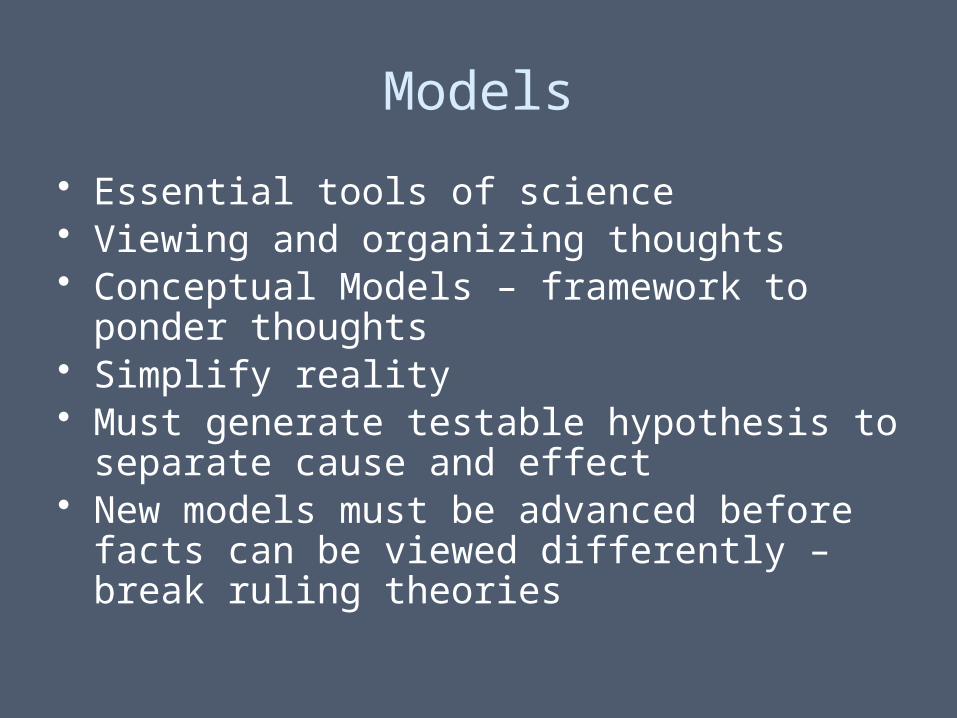
Models

• Essential tools of science• Viewing and organizing thoughts• Conceptual Models – framework to ponder

thoughts• Simplify reality• Must generate testable hypothesis to separate

cause and effect• New models must be advanced before facts can

be viewed differently – break ruling theories

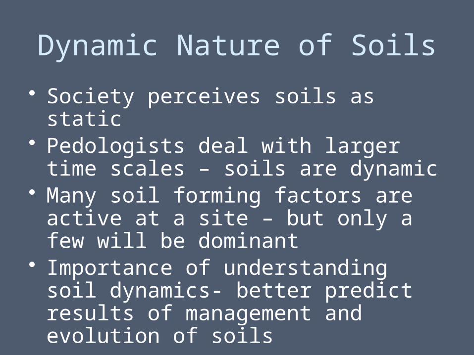
Dynamic Nature of Soils

• Society perceives soils as static• Pedologists deal with larger time scales –

soils are dynamic• Many soil forming factors are active at a

site – but only a few will be dominant• Importance of understanding soil

dynamics- better predict results of management and evolution of soils

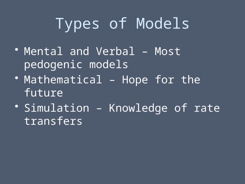
Types of Models

• Mental and Verbal – Most pedogenic models

• Mathematical – Hope for the future• Simulation – Knowledge of rate transfers

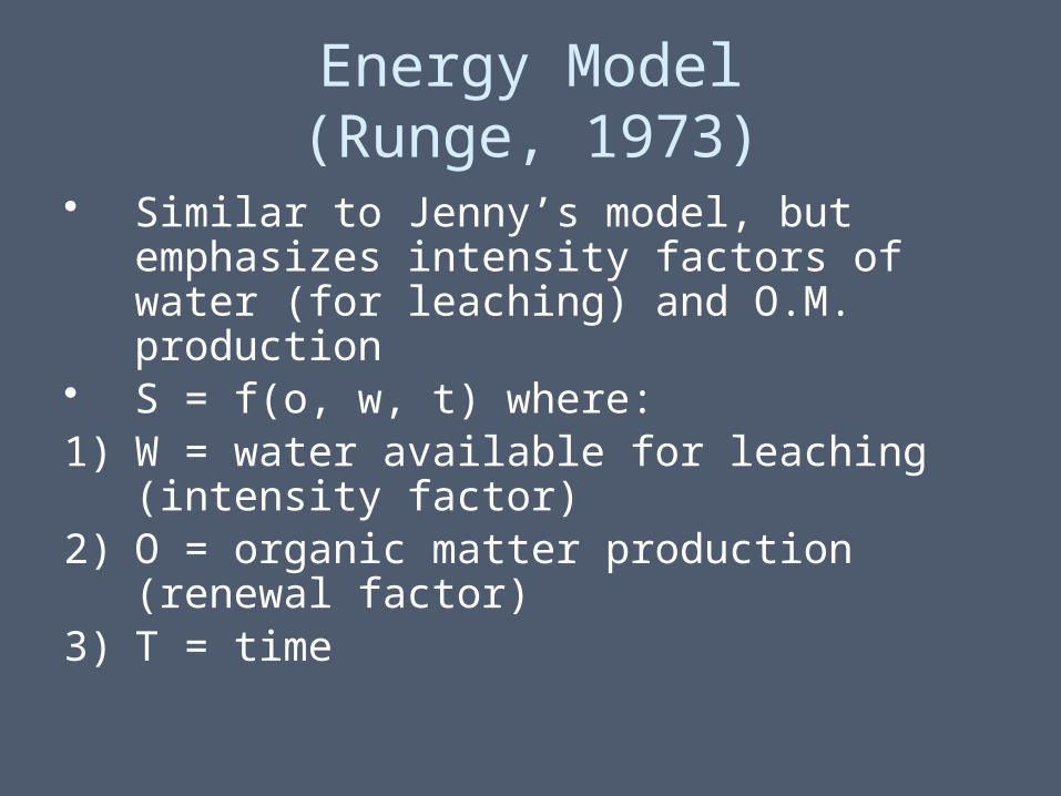
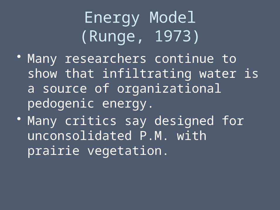
Energy Model(Runge, 1973)

• Similar to Jenny’s model, but emphasizes intensity factors of water (for leaching) and O.M. production

• S = f(o, w, t) where:1) W = water available for leaching (intensity

factor)2) O = organic matter production (renewal factor)3) T = time

Energy Model(Runge, 1973)

• Many researchers continue to show that infiltrating water is a source of organizational pedogenic energy.

• Many critics say designed for unconsolidated P.M. with prairie vegetation.

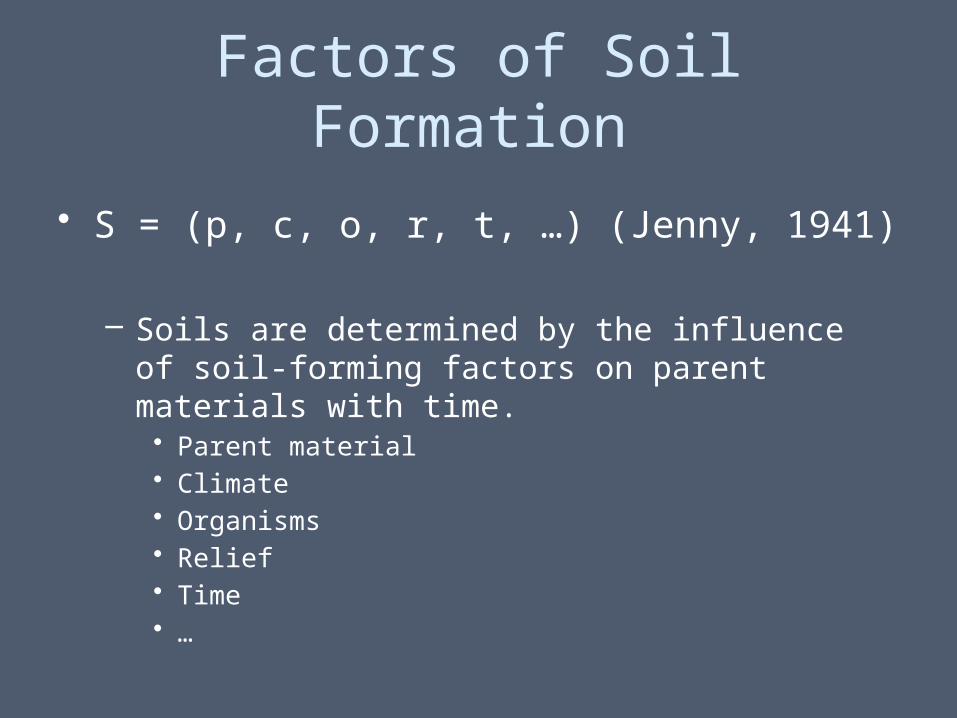
Factors of Soil Formation

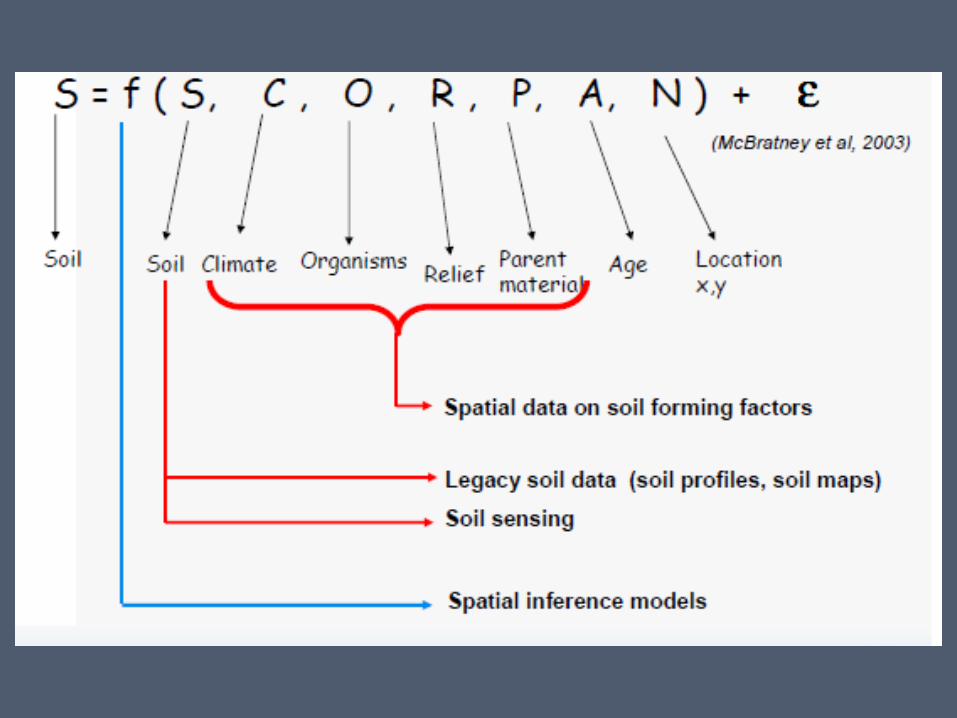
• S = (p, c, o, r, t, …) (Jenny, 1941)

– Soils are determined by the influence of soil-forming factors on parent materials with time.• Parent material• Climate• Organisms• Relief• Time• …

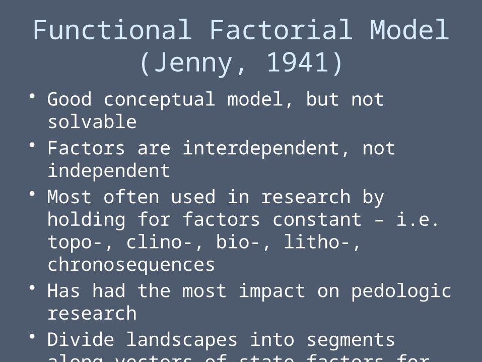
Functional Factorial Model(Jenny, 1941)

• Good conceptual model, but not solvable• Factors are interdependent, not independent• Most often used in research by holding for

factors constant – i.e. topo-, clino-, bio-, litho-, chronosequences

• Has had the most impact on pedologic research• Divide landscapes into segments along vectors

of state factors for better understanding

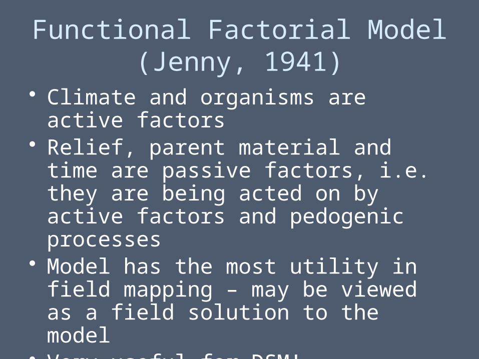
Functional Factorial Model(Jenny, 1941)

• Climate and organisms are active factors• Relief, parent material and time are

passive factors, i.e. they are being acted on by active factors and pedogenic processes

• Model has the most utility in field mapping – may be viewed as a field solution to the model

• Very useful for DSM!

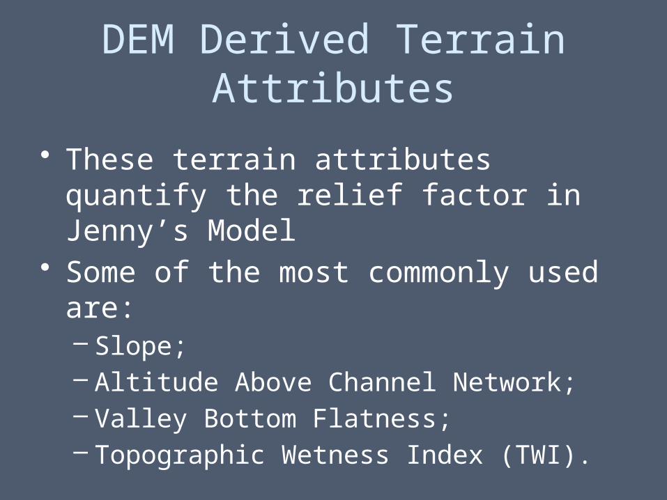
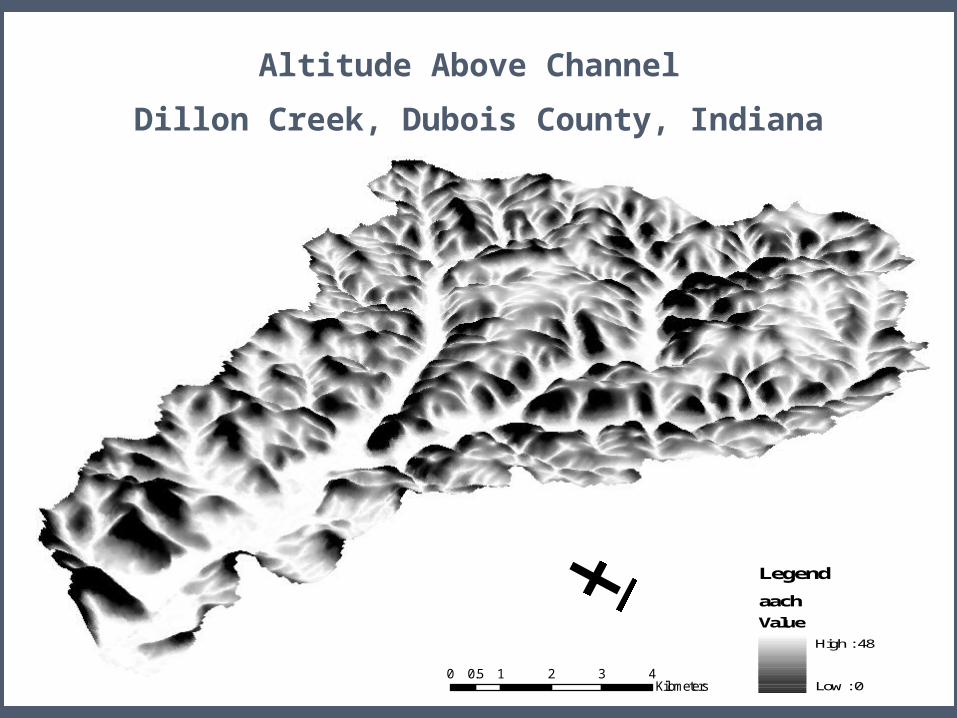
DEM Derived Terrain Attributes

• These terrain attributes quantify the relief factor in Jenny’s Model

• Some of the most commonly used are:– Slope;– Altitude Above Channel Network;– Valley Bottom Flatness;– Topographic Wetness Index (TWI).

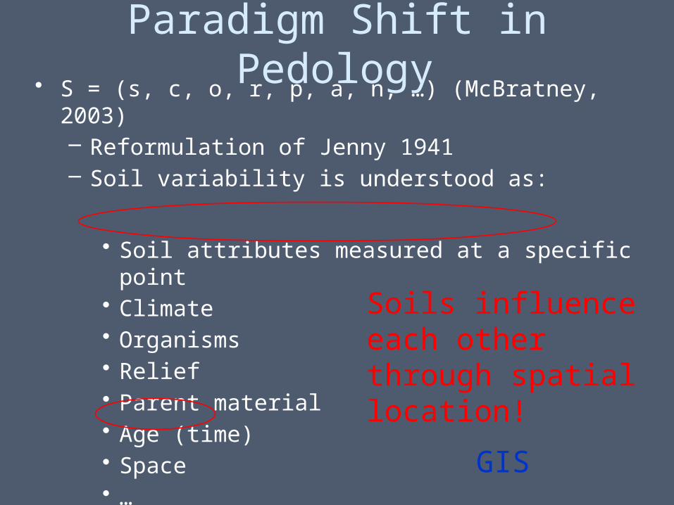
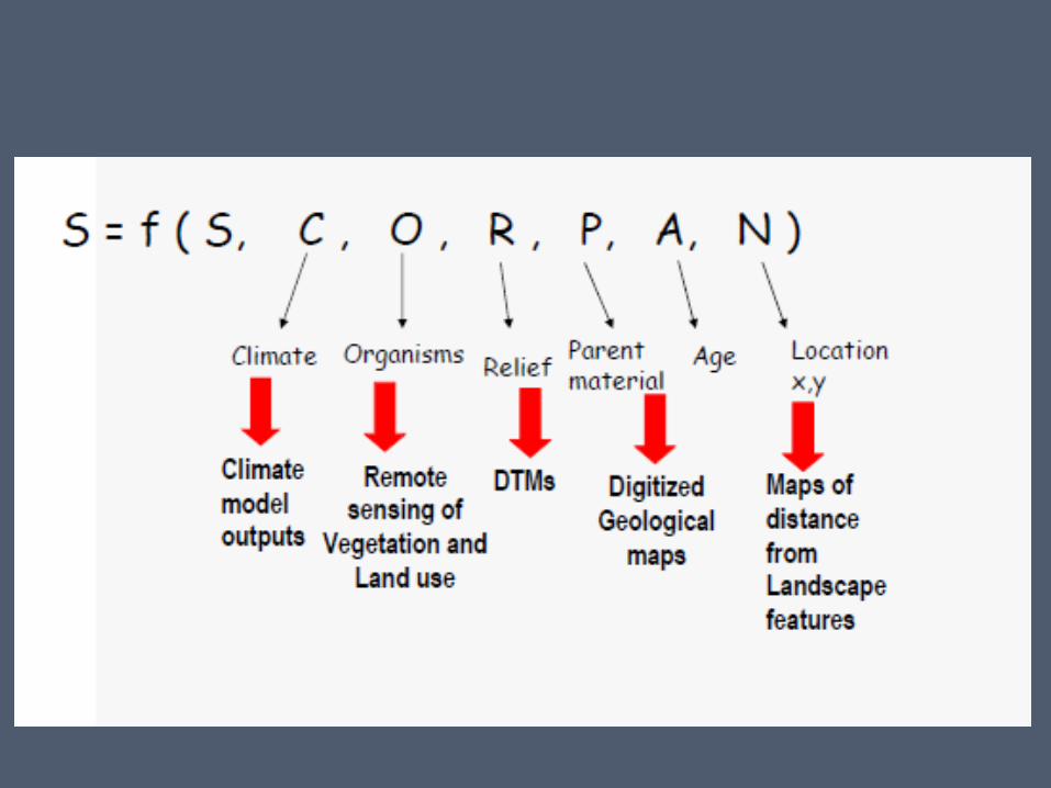
Paradigm Shift in Pedology• S = (s, c, o, r, p, a, n, …) (McBratney, 2003)

– Reformulation of Jenny 1941– Soil variability is understood as:

• Soil attributes measured at a specific point• Climate• Organisms• Relief• Parent material• Age (time)• Space• …

Soils influence each other through spatial location!

GIS

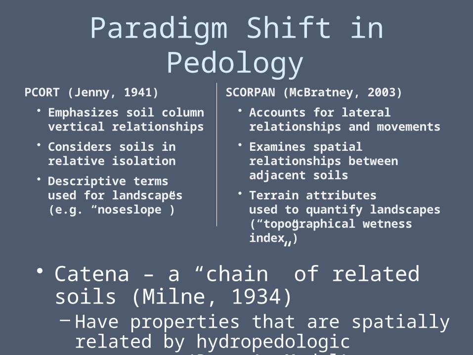
Paradigm Shift in Pedology

PCORT (Jenny, 1941)

• Emphasizes soil column vertical relationships

• Considers soils in relative isolation

• Descriptive terms used for landscapes (e.g. “noseslope”)

SCORPAN (McBratney, 2003)

• Accounts for lateral relationships and movements

• Examines spatial relationships between adjacent soils

• Terrain attributesused to quantify landscapes(“topographical wetness index”)

• Catena – a “chain” of related soils (Milne, 1934)– Have properties that are spatially related by

hydropedologic processes (Runge’s Model)

19

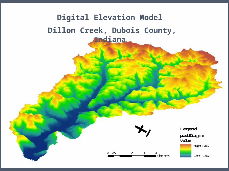
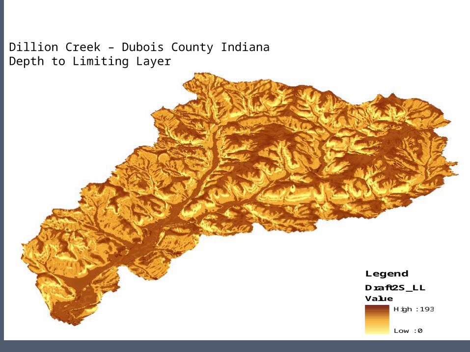
Digital Elevation Model

Dillon Creek, Dubois County, Indiana

Legend

padillcr_mm

Value

High : 267

Low : 146

Elevation

m

m0 1 2 3 40.5Kilometers

±

200 1 2 3 40.5Kilometers

±

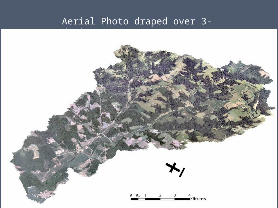
Aerial Photo draped over 3-d view

21

AACH

Altitude Above Channel

Dillon Creek, Dubois County, Indiana

Legend

aach

Value

High : 48

Low : 00 1 2 3 40.5

Kilometers

±

22

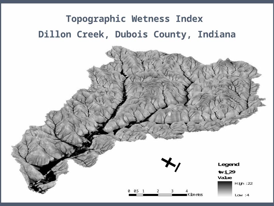
TWI

Topographic Wetness Index

Dillon Creek, Dubois County, Indiana

Legend

twi_29

Value

High : 22

Low : 40 1 2 3 40.5

Kilometers

±

23

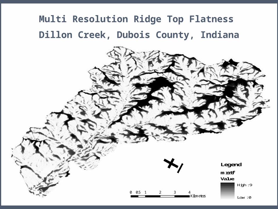
MRRTFLegend

mrrtf

Value

High : 9

Low : 0

Multi Resolution Ridge Top Flatness

Dillon Creek, Dubois County, Indiana

0 1 2 3 40.5Kilometers

±

24

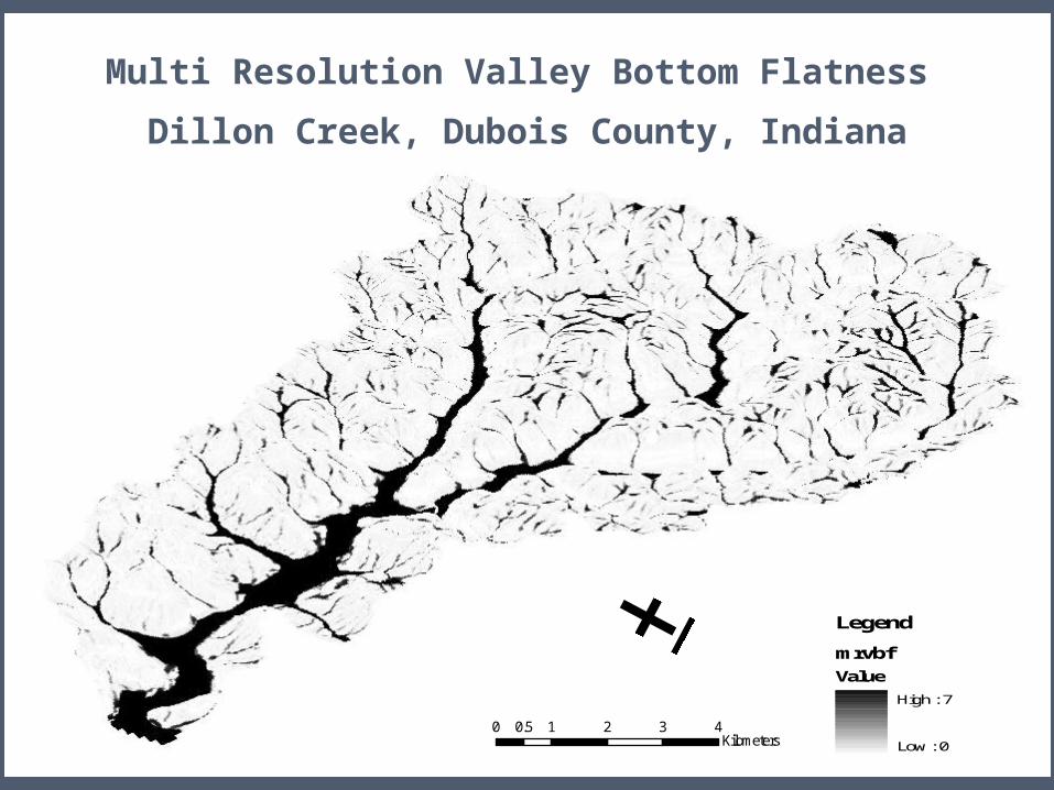
MRVBFLegend

mrvbf

Value

High : 7

Low : 0

Multi Resolution Valley Bottom Flatness

Dillon Creek, Dubois County, Indiana

0 1 2 3 40.5Kilometers

±

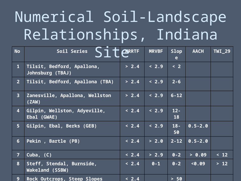
No Soil Series MRRTF MRVBF Slope AACH TWI_29

1 Tilsit, Bedford, Apallona, Johnsburg (TBAJ) > 2.4 < 2.9 < 2

2 Tilsit, Bedford, Apallona (TBA) > 2.4 < 2.9 2-6

3 Zanesville, Apallona, Wellston (ZAW) > 2.4 < 2.9 6-12

4 Gilpin, Wellston, Adyeville, Ebal (GWAE) < 2.4 < 2.9 12-18

5 Gilpin, Ebal, Berks (GEB) < 2.4 < 2.9 18-50 0.5-2.0

6 Pekin , Bartle (PB) < 2.4 > 2.0 2-12 0.5-2.0

7 Cuba, (C) < 2.4 > 2.9 0-2 > 0.09 < 12

8 Steff, Stendal, Burnside, Wakeland (SSBW) < 2.4 0-1 0-2 <0.09 > 12

9 Rock Outcrops, Steep Slopes < 2.4 > 50

Numerical Soil-Landscape Relationships, Indiana Site

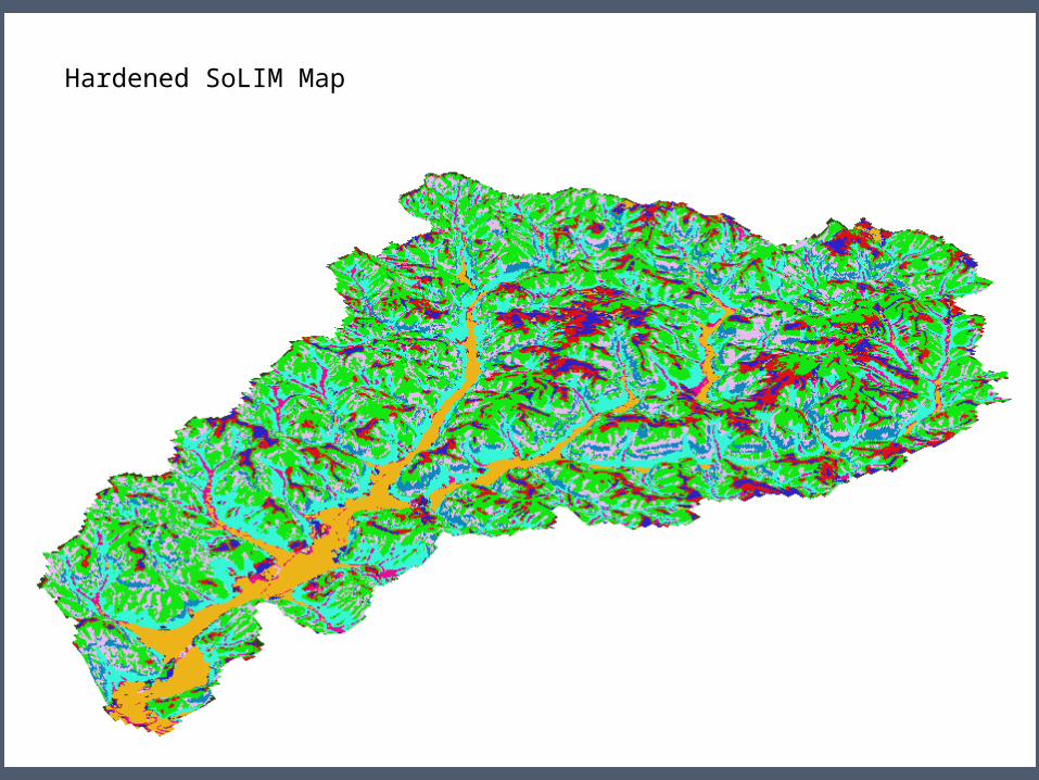
SOLIM map

Hardened SoLIM Map

Dillion Creek – Dubois County IndianaDepth to Limiting Layer

Legend

Draft2S_LL

Value

High : 193

Low : 0

cm

cm

Low relief Landscape in the Glaciated Portion of Indiana

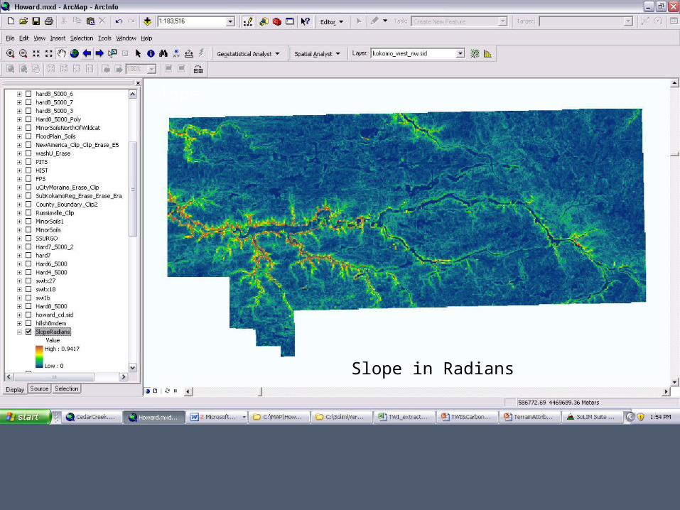
Slope

Slope in Radians

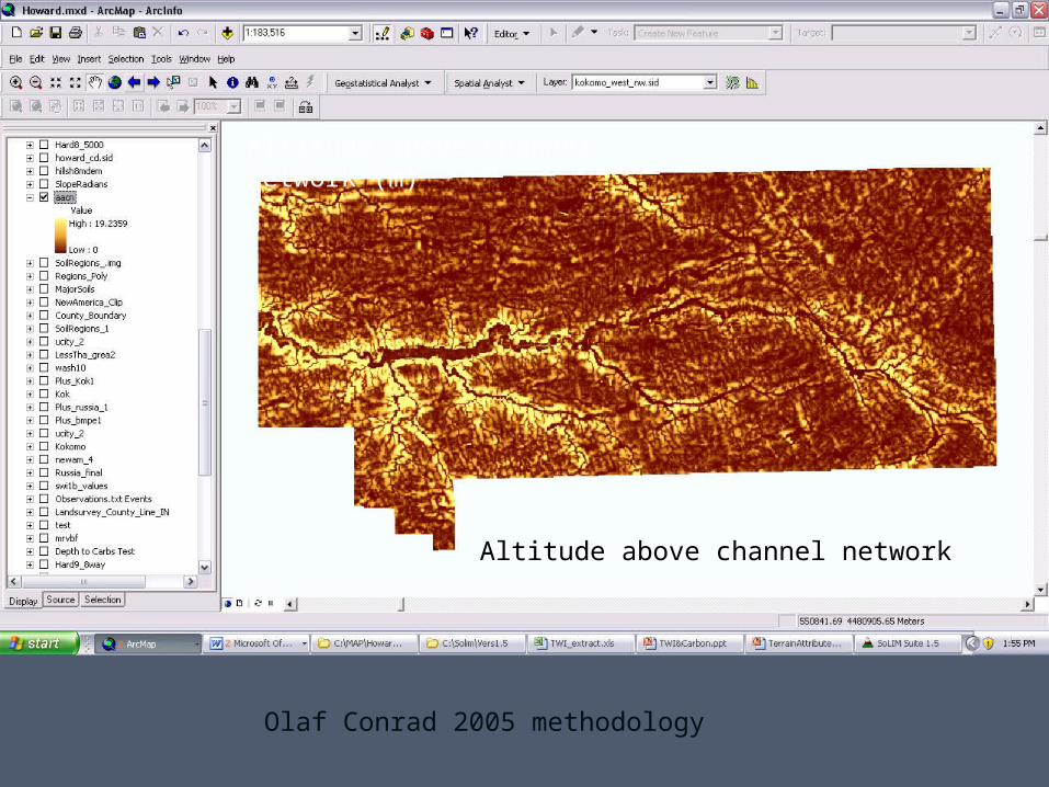
Altitude above channel network (m)

Olaf Conrad 2005 methodology

Altitude above channel network

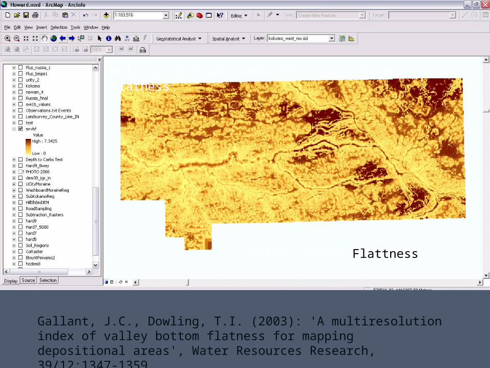
Multi-resolution index of valley-bottom flatness

Gallant, J.C., Dowling, T.I. (2003): 'A multiresolution index of valley bottom flatness for mapping depositional areas', Water Resources Research, 39/12:1347-1359

Valley Bottom Flattness

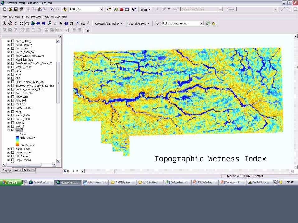
TWI: 9

Topographic Wetness Index

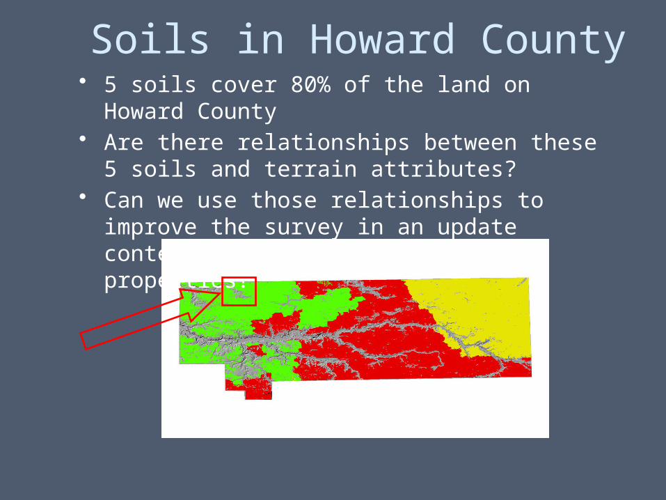
Soils in Howard County• 5 soils cover 80% of the land on Howard County• Are there relationships between these 5 soils and

terrain attributes?• Can we use those relationships to improve the

survey in an update context? Provide predicted properties?

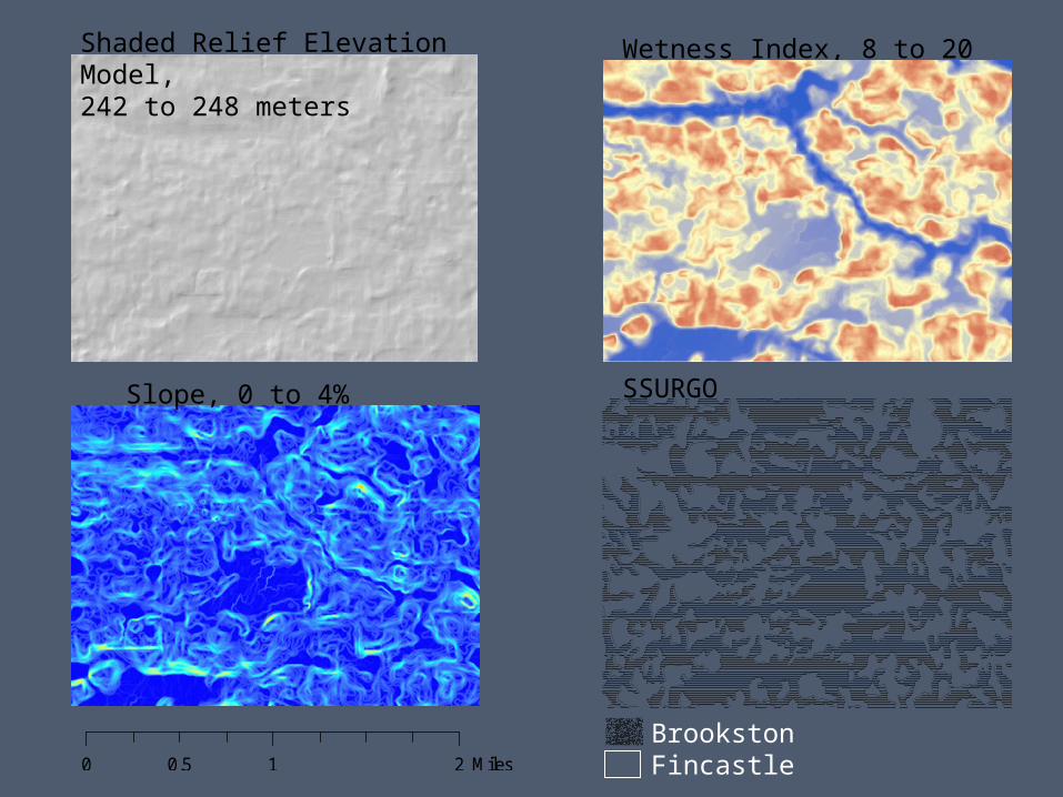
SSURGO

Shaded Relief Elevation Model, 242 to 248 meters

Brookston Fincastle

Wetness Index, 8 to 20

Slope, 0 to 4%

0 1 20.5 Miles

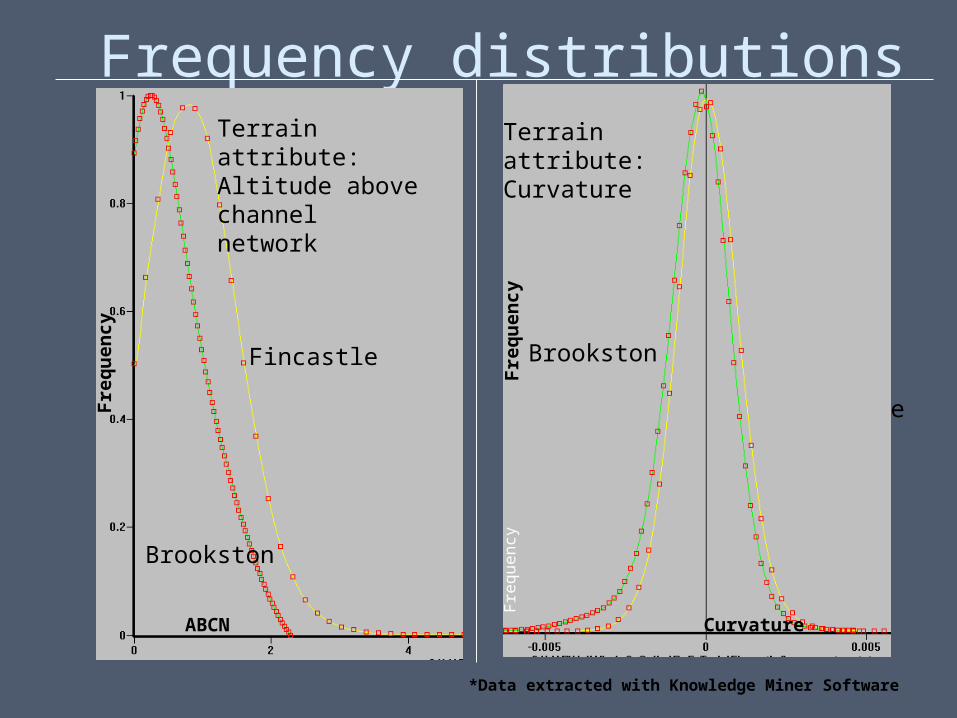
Frequency distributions

Fincastle

Terrain attribute:Curvature

Brookston

Terrain attribute:Altitude above channel network

Brookston

Fincastle

Fre

qu

enc

y

Fre

qu

en

cyF

req

uen

cy

ABCN Curvature

*Data extracted with Knowledge Miner Software

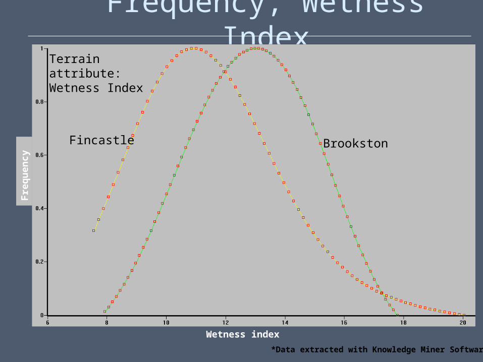
Frequency, Wetness IndexF

req

uen

cy

BrookstonFincastle

Terrain attribute:Wetness Index

Wetness index

*Data extracted with Knowledge Miner Software

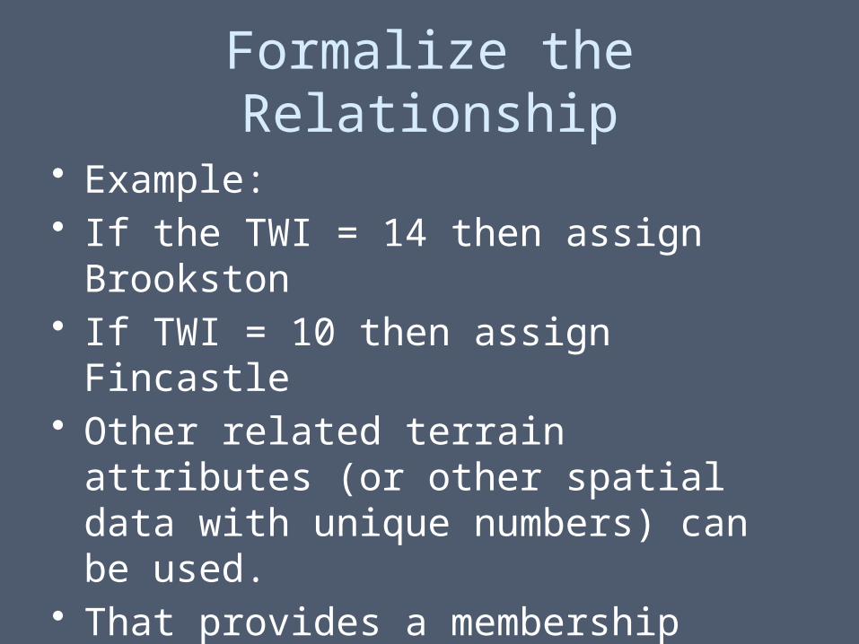
Formalize the Relationship

• Example: • If the TWI = 14 then assign Brookston• If TWI = 10 then assign Fincastle• Other related terrain attributes (or other

spatial data with unique numbers) can be used.

• That provides a membership probability to each pixel

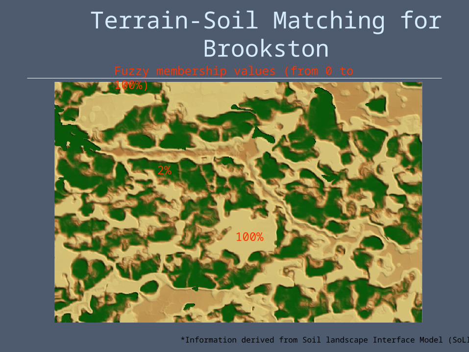
Terrain-Soil Matching for Brookston

100%

2%

Fuzzy membership values (from 0 to 100%)

*Information derived from Soil landscape Interface Model (SoLIM)

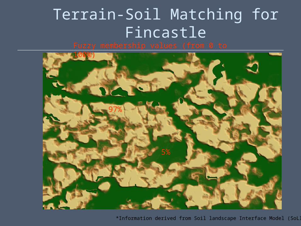
Terrain-Soil Matching for Fincastle

5%

97%

Fuzzy membership values (from 0 to 100%)

*Information derived from Soil landscape Interface Model (SoLIM)

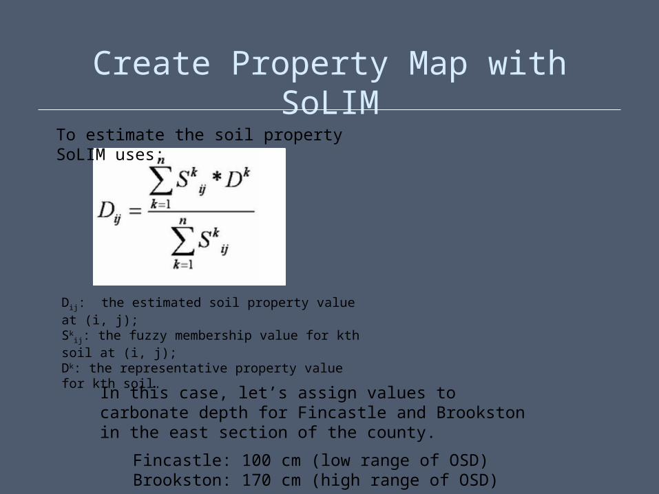
Create Property Map with SoLIM

Dij: the estimated soil property value at (i, j);Sk

ij: the fuzzy membership value for kth soil at (i, j);Dk: the representative property value for kth soil.

We already have Skij – the

fuzzy membership value used to make the hardened soil map.

To estimate the soil property SoLIM uses:

In this case, let’s assign values to carbonate depth for Fincastle and Brookston in the east section of the county.

Fincastle: 100 cm (low range of OSD)Brookston: 170 cm (high range of OSD)

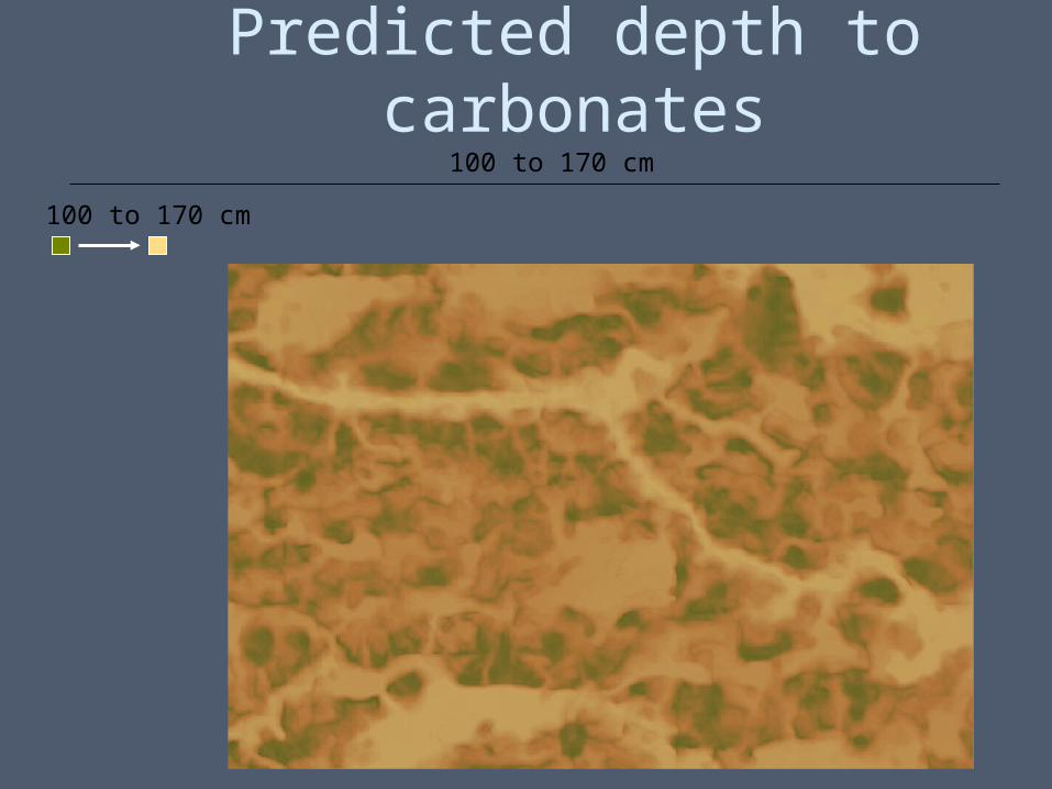
Predicted depth to carbonates100 to 170 cm

100 to 170 cm

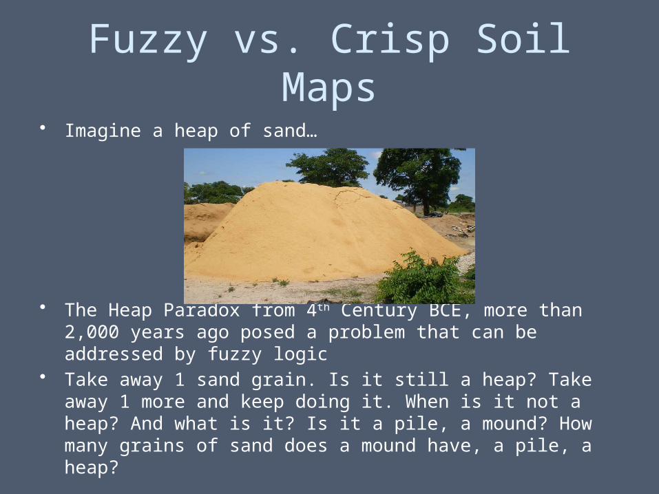
Fuzzy vs. Crisp Soil Maps

• Imagine a heap of sand…

• The Heap Paradox from 4th Century BCE, more than 2,000 years ago posed a problem that can be addressed by fuzzy logic

• Take away 1 sand grain. Is it still a heap? Take away 1 more and keep doing it. When is it not a heap? And what is it? Is it a pile, a mound? How many grains of sand does a mound have, a pile, a heap?

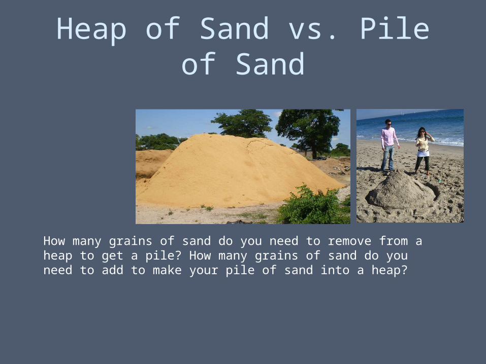
Heap of Sand vs. Pile of Sand

How many grains of sand do you need to remove from a heap to get a pile? How many grains of sand do you need to add to make your pile of sand into a heap?

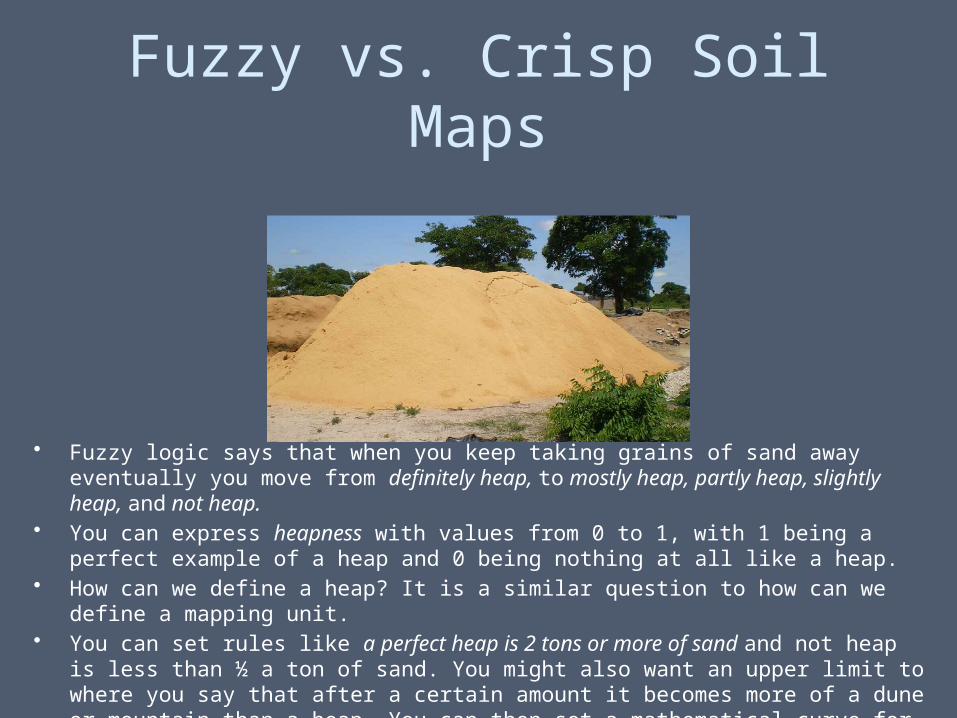
Fuzzy vs. Crisp Soil Maps

• Fuzzy logic says that when you keep taking grains of sand away eventually you move from definitely heap, to mostly heap, partly heap, slightly heap, and not heap.

• You can express heapness with values from 0 to 1, with 1 being a perfect example of a heap and 0 being nothing at all like a heap.

• How can we define a heap? It is a similar question to how can we define a mapping unit.• You can set rules like a perfect heap is 2 tons or more of sand and not heap is less than ½

a ton of sand. You might also want an upper limit to where you say that after a certain amount it becomes more of a dune or mountain than a heap. You can then set a mathematical curve for expressing the decline in heapness as a function of the removal of sand grains.

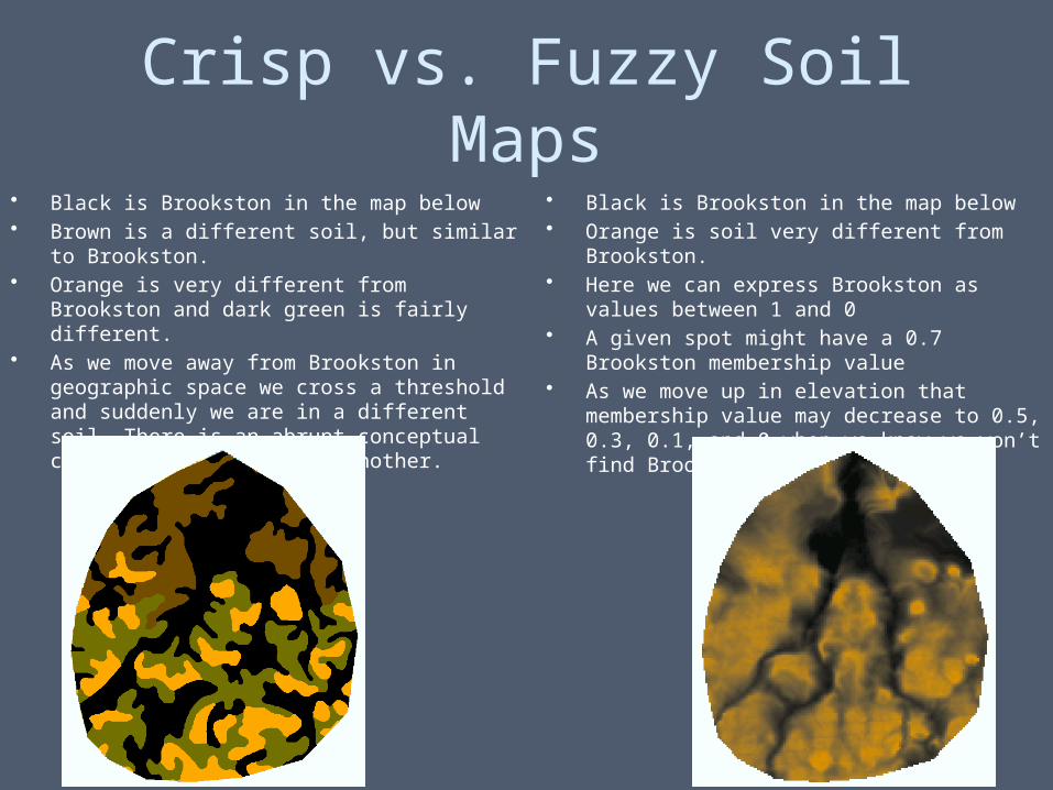
• Black is Brookston in the map below• Orange is soil very different from Brookston. • Here we can express Brookston as values

between 1 and 0• A given spot might have a 0.7 Brookston

membership value• As we move up in elevation that membership

value may decrease to 0.5, 0.3, 0.1, and 0 when we know we won’t find Brookston

• Black is Brookston in the map below• Brown is a different soil, but similar to Brookston. • Orange is very different from Brookston and dark

green is fairly different.• As we move away from Brookston in geographic

space we cross a threshold and suddenly we are in a different soil. There is an abrupt conceptual change from one soil to another.

Crisp vs. Fuzzy Soil Maps

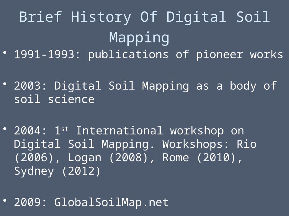
Brief History Of Digital Soil Mapping • 1991-1993: publications of pioneer works

• 2003: Digital Soil Mapping as a body of soil science

• 2004: 1st International workshop on Digital Soil Mapping. Workshops: Rio (2006), Logan (2008), Rome (2010), Sydney (2012)

• 2009: GlobalSoilMap.net

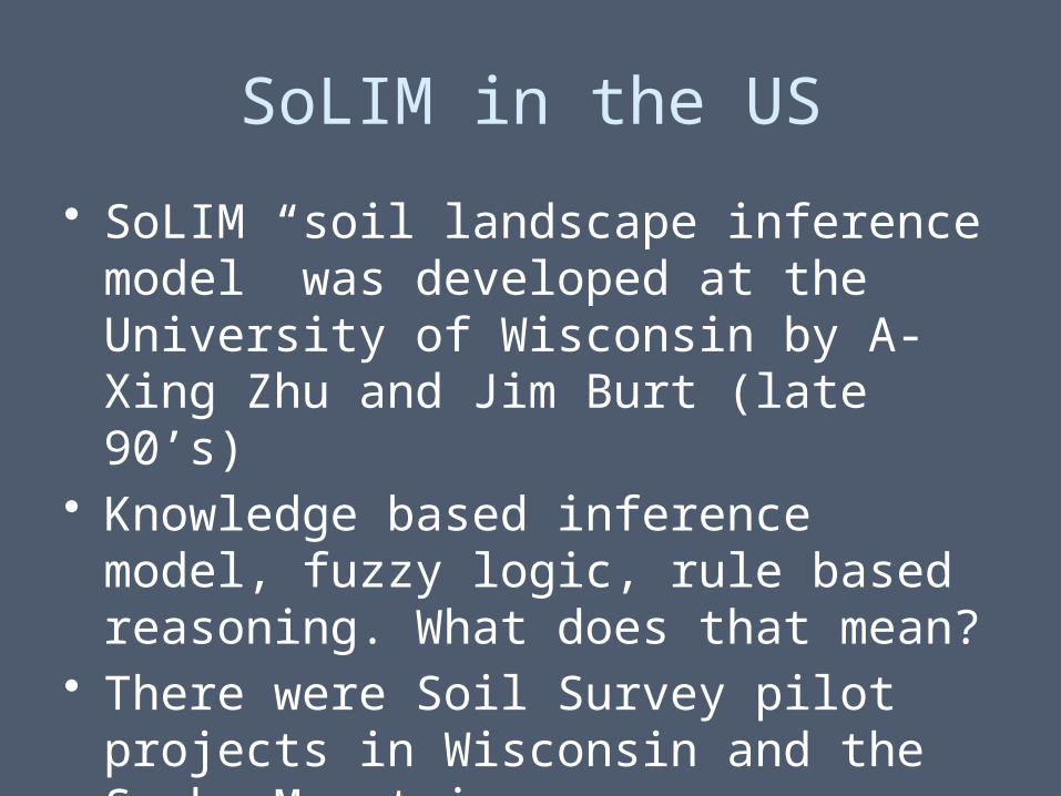
SoLIM in the US

• SoLIM “soil landscape inference model” was developed at the University of Wisconsin by A-Xing Zhu and Jim Burt (late 90’s)

• Knowledge based inference model, fuzzy logic, rule based reasoning. What does that mean?

• There were Soil Survey pilot projects in Wisconsin and the Smoky Mountains

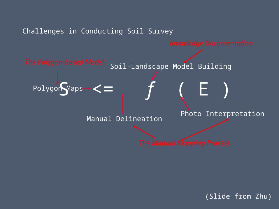
Challenges in Conducting Soil Survey

S <= f ( E )

Soil-Landscape Model Building

Photo InterpretationManual Delineation

Polygon Maps

The Polygon-based Model

The Manual Mapping Process

Knowledge Documentation

(Slide from Zhu)

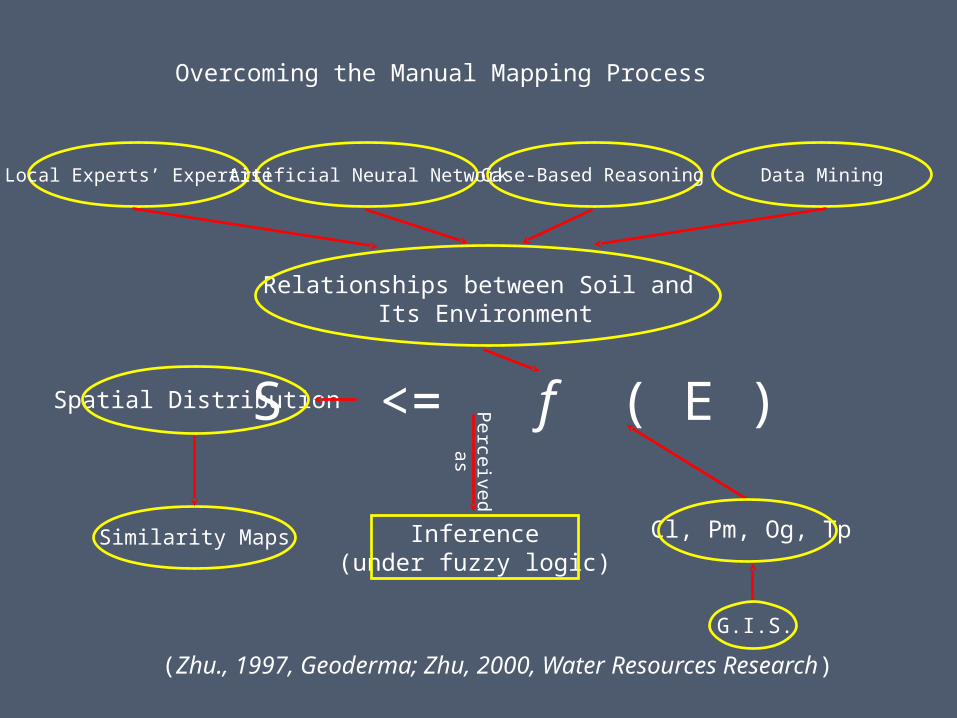
Spatial Distribution

Similarity Maps Inference(under fuzzy logic)

Perceived

as

S <= f ( E )

Relationships between Soil and Its Environment

Cl, Pm, Og, Tp

G.I.S.

Local Experts’ Expertise Artificial Neural Network Data MiningCase-Based Reasoning

(Zhu., 1997, Geoderma; Zhu, 2000, Water Resources Research)

Overcoming the Manual Mapping Process

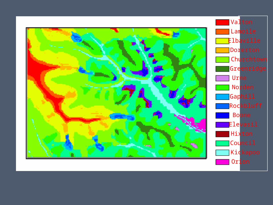
Valton

Lamoile

Elbaville

Dorerton

Churchtown

Greenridge

Urne

Norden

Gaphill

Rockbluff

Boone

Elevasil

Hixton

Council

Kickapoo

Orion

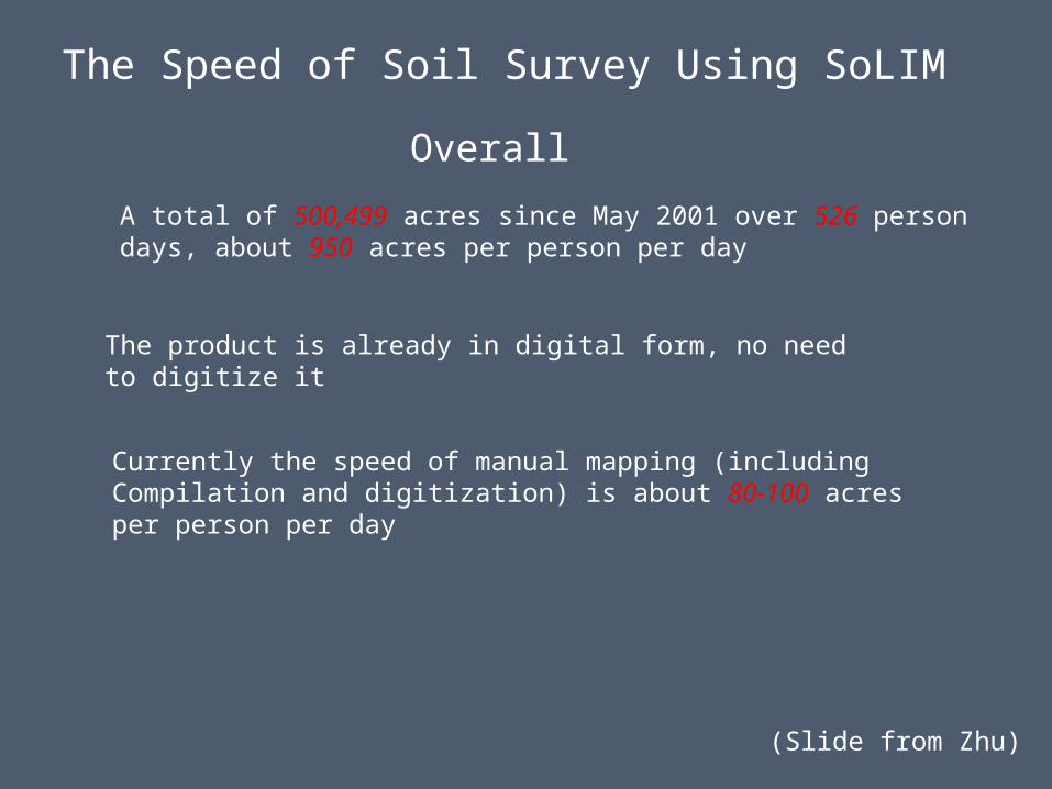
The Speed of Soil Survey Using SoLIM

The product is already in digital form, no need to digitize it

A total of 500,499 acres since May 2001 over 526 person days, about 950 acres per person per day

Overall

Currently the speed of manual mapping (including Compilation and digitization) is about 80-100 acres per person per day

(Slide from Zhu)

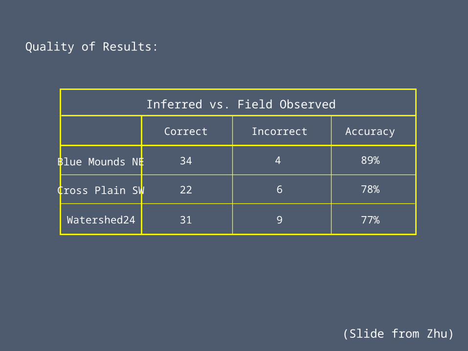
Quality of Results:

Inferred vs. Field Observed

Correct Incorrect Accuracy

Blue Mounds NE

Cross Plain SW

34

22

4

6

89%

78%

Watershed24 31 9 77%

(Slide from Zhu)

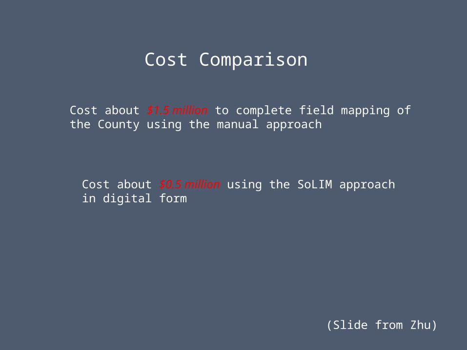
Cost Comparison

Cost about $1.5 million to complete field mapping of the County using the manual approach

Cost about $0.5 million using the SoLIM approachin digital form

(Slide from Zhu)

SoLIM

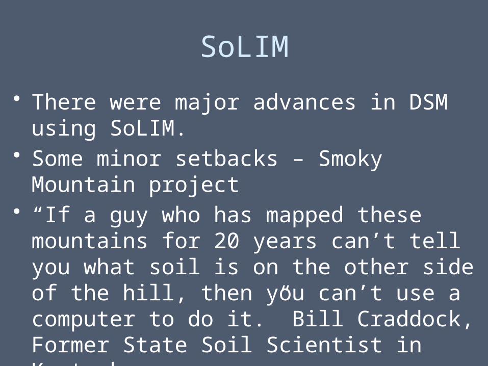
• There were major advances in DSM using SoLIM.

• Some minor setbacks – Smoky Mountain project

• “If a guy who has mapped these mountains for 20 years can’t tell you what soil is on the other side of the hill, then you can’t use a computer to do it.” Bill Craddock, Former State Soil Scientist in Kentucky

DSM – Current State

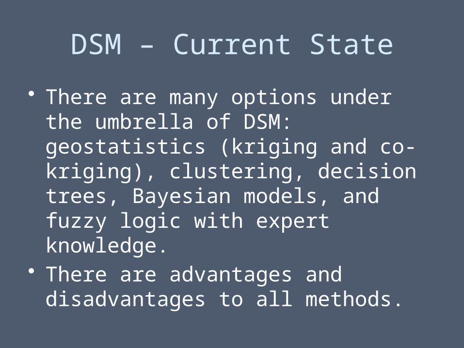
• There are many options under the umbrella of DSM: geostatistics (kriging and co-kriging), clustering, decision trees, Bayesian models, and fuzzy logic with expert knowledge.

• There are advantages and disadvantages to all methods.

DSM – Current State

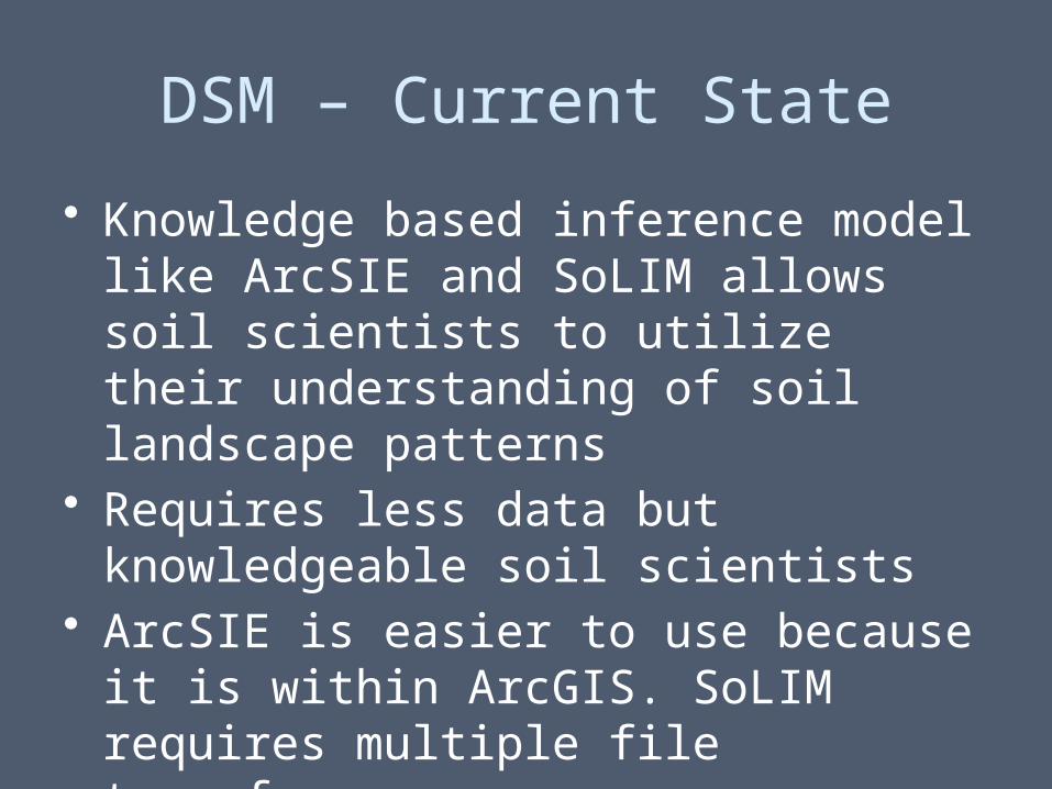
• Knowledge based inference model like ArcSIE and SoLIM allows soil scientists to utilize their understanding of soil landscape patterns

• Requires less data but knowledgeable soil scientists

• ArcSIE is easier to use because it is within ArcGIS. SoLIM requires multiple file transfers

DSM Current State

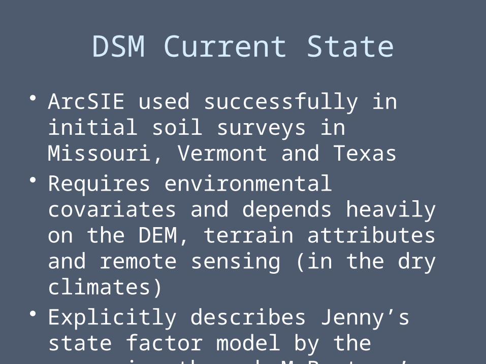
• ArcSIE used successfully in initial soil surveys in Missouri, Vermont and Texas

• Requires environmental covariates and depends heavily on the DEM, terrain attributes and remote sensing (in the dry climates)

• Explicitly describes Jenny’s state factor model by the expansion through McBratney’s SCORPAN

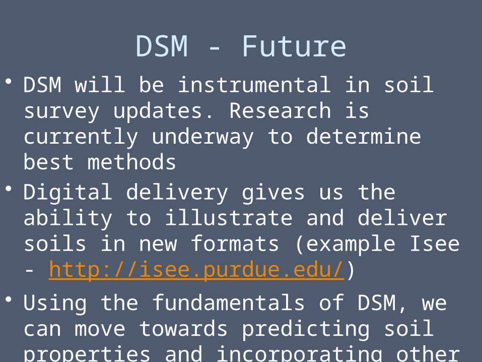
DSM - Future• DSM will be instrumental in soil survey updates.

Research is currently underway to determine best methods

• Digital delivery gives us the ability to illustrate and deliver soils in new formats (example Isee - http://isee.purdue.edu/)

• Using the fundamentals of DSM, we can move towards predicting soil properties and incorporating other explanatory data (i.e. ecologic site descriptions, land use, etc.)

Dillion Creek – Dubois County IndianaDepth to Limiting Layer

Legend

Draft2S_LL

Value

High : 193

Low : 0

cm

cm

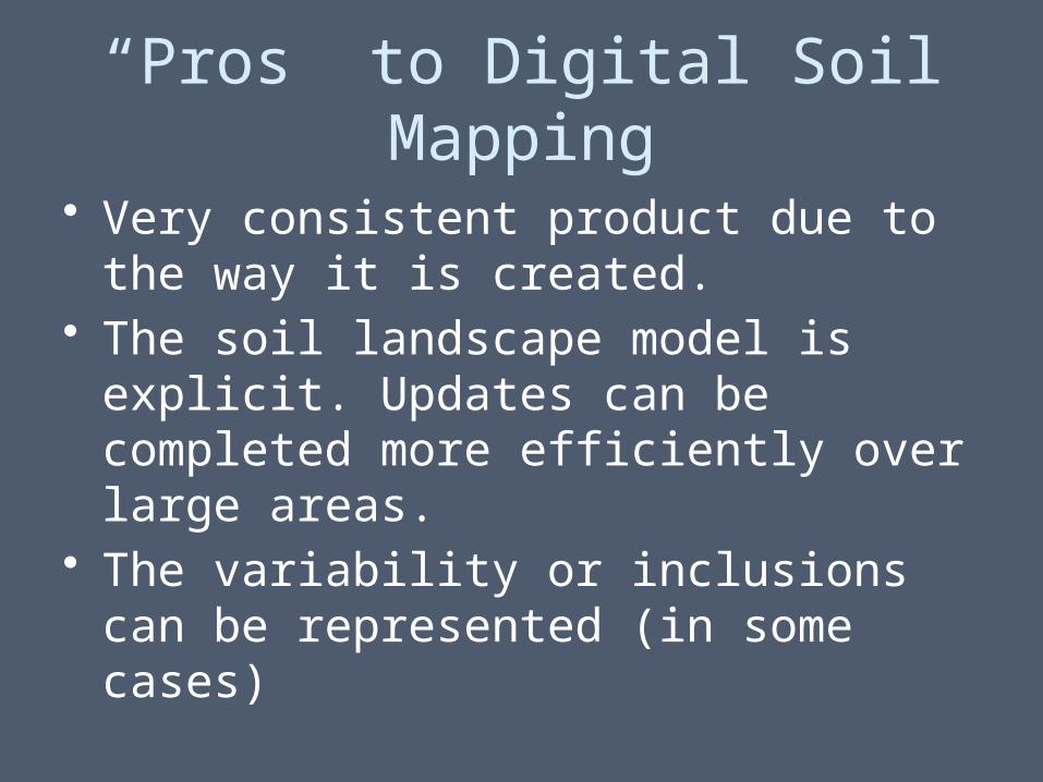
“Pros” to Digital Soil Mapping

• Very consistent product due to the way it is created.

• The soil landscape model is explicit. Updates can be completed more efficiently over large areas.

• The variability or inclusions can be represented (in some cases)

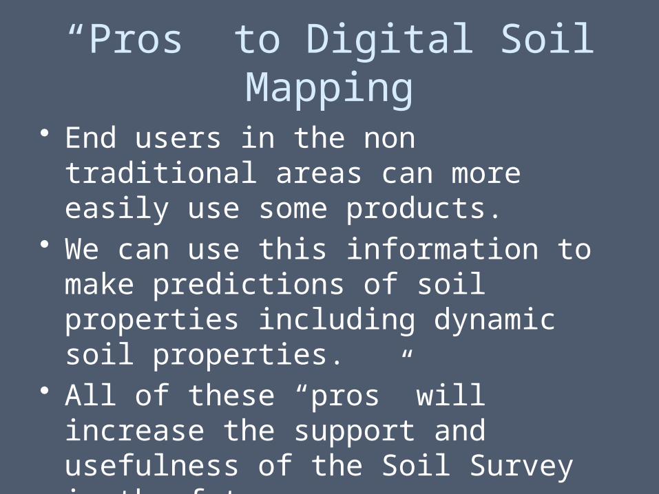
“Pros” to Digital Soil Mapping

• End users in the non traditional areas can more easily use some products.

• We can use this information to make predictions of soil properties including dynamic soil properties.

• All of these “pros” will increase the support and usefulness of the Soil Survey in the future.

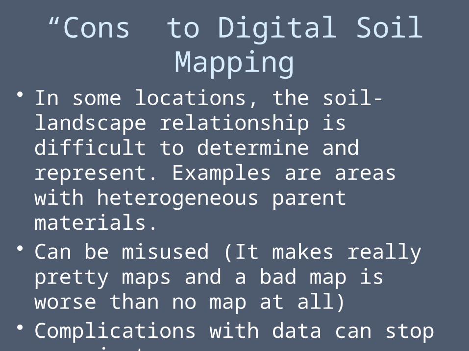
“Cons” to Digital Soil Mapping

• In some locations, the soil-landscape relationship is difficult to determine and represent. Examples are areas with heterogeneous parent materials.

• Can be misused (It makes really pretty maps and a bad map is worse than no map at all)

• Complications with data can stop a project. • Learning new softwares can be very

frustrating

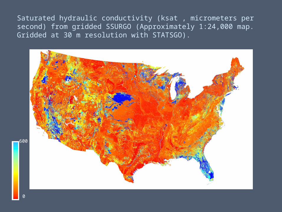
Saturated hydraulic conductivity (ksat , micrometers per second) from gridded SSURGO (Approximately 1:24,000 map. Gridded at 30 m resolution with STATSGO).

600

0

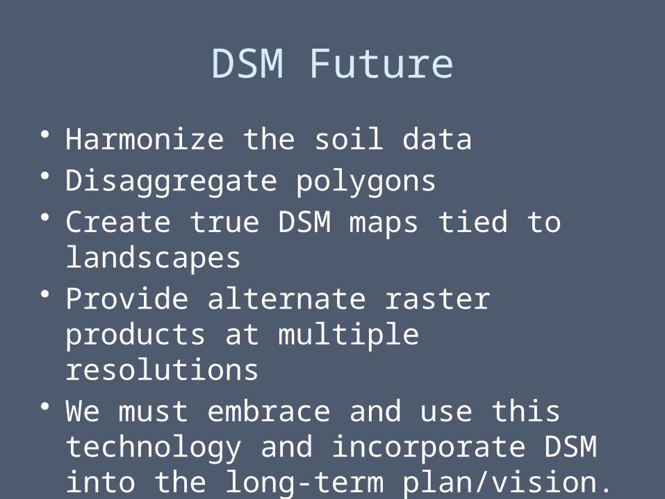
DSM Future

• Harmonize the soil data• Disaggregate polygons • Create true DSM maps tied to landscapes• Provide alternate raster products at

multiple resolutions• We must embrace and use this technology

and incorporate DSM into the long-term plan/vision.