Embed Size (px)
Citation preview

Digital CommunicationsChapter 3: Digital Modulation Schemes
Po-Ning Chen, Professor
Institute of Communications EngineeringNational Chiao-Tung University, Taiwan
Digital Communications: Chapter 3 Ver. 2016.04.09 Po-Ning Chen 1 / 160
3.1 Representation of digitallymodulated signals
Digital Communications: Chapter 3 Ver. 2016.04.09 Po-Ning Chen 2 / 160

Note that the channel symbols are bandpass signals.
Digital Communications: Chapter 3 Ver. 2016.04.09 Po-Ning Chen 3 / 160

L = Constraint length of mod-ulation (with memory)
Memoryless modulation: sm`(t), m` ∈ {1,2, . . . ,M},m` =function of Block`
Modulation with memory: sm`(t),m` =function of (Block`, Block`−1,⋯, Block`−(L−1))
Digital Communications: Chapter 3 Ver. 2016.04.09 Po-Ning Chen 4 / 160

Terminology
Signal sm(t), 1 ≤ m ≤M , t ∈ [0,Ts)
Signaling interval: Ts (For convenience, we will use Tinstead sometimes.)
Signaling rate (or symbol rate): Rs =1Ts
(Equivalent) Bit interval: Tb =Ts
log2 M
(Eqiuvalent) Bit rate: Rb =1Tb
= Rs log2 M
Average signal energy (assume equal-probable in messagem)
Eavg =1
M
M
∑m=1∫
Ts
0∣sm(t)∣
2dt
(Equivalent) Average bit energy: Ebavg =Eavg
log2 M
Average power: Pavg =Eavg
Ts= RsEavg =
Ebavg
Tb= RbEbavg
Digital Communications: Chapter 3 Ver. 2016.04.09 Po-Ning Chen 5 / 160

3.2 Memoryless modulationmethods
Digital Communications: Chapter 3 Ver. 2016.04.09 Po-Ning Chen 6 / 160

Example studies of memoryless modulation
Digital pulse amplitude modulated (PAM) signals(Amplitude-shift keying or ASK)
Digital phase-modulated (PM) signals (Phase shift keyingor PSK)
Quadrature amplitude modulated (QAM) signals
Multidimensional modulated signals
OrthogonalBi-orthogonal
Simplex signals
Digital Communications: Chapter 3 Ver. 2016.04.09 Po-Ning Chen 7 / 160

M-ary pulse amplitude modulation (M-PAM)
PAM bandpass waveform
sm(t) = Re{Amg(t)eı2πfc t} = Amg(t) cos (2πfct) , t ∈ [0,Ts),
where Am = (2m − 1 −M)d , and m = 1,2,⋯,M
Example 1 (M=4)
⎧⎪⎪⎪⎪⎪⎨⎪⎪⎪⎪⎪⎩
s1(t) = −3 ⋅ d ⋅ g(t) ⋅ cos (2πfct)s2(t) = −1 ⋅ d ⋅ g(t) ⋅ cos (2πfct)s3(t) = +1 ⋅ d ⋅ g(t) ⋅ cos (2πfct)s4(t) = +3 ⋅ d ⋅ g(t) ⋅ cos (2πfct)
The amplitude difference between two adjacent signals = 2d .
Digital Communications: Chapter 3 Ver. 2016.04.09 Po-Ning Chen 8 / 160

sm(t) = Re{Amg(t)e ı2πfc t} = Amg(t) cos (2πfct) , t ∈ [0,Ts)
g(t) is the pulse shaping function.
Ts is usually assumed to be a multiple of 1fc
in principle.
Digital Communications: Chapter 3 Ver. 2016.04.09 Po-Ning Chen 9 / 160
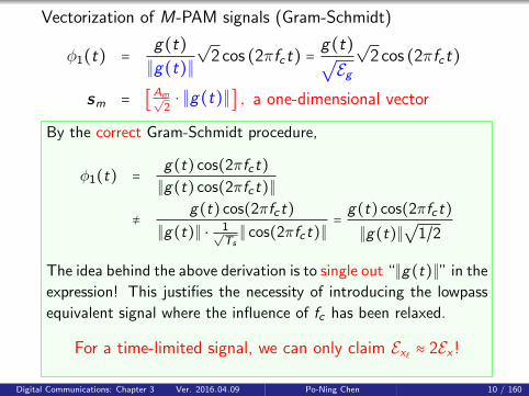
Vectorization of M-PAM signals (Gram-Schmidt)
φ1(t) =g(t)
∥g(t)∥
√2 cos (2πfct) =
g(t)√Eg
√2 cos (2πfct)
sm = [Am√
2⋅ ∥g(t)∥] , a one-dimensional vector
By the correct Gram-Schmidt procedure,
φ1(t) =g(t) cos(2πfct)
∥g(t) cos(2πfct)∥
≠g(t) cos(2πfct)
∥g(t)∥ ⋅ 1√Ts
∥ cos(2πfct)∥=g(t) cos(2πfct)
∥g(t)∥√
1/2
The idea behind the above derivation is to single out “∥g(t)∥” in the
expression! This justifies the necessity of introducing the lowpass
equivalent signal where the influence of fc has been relaxed.
For a time-limited signal, we can only claim Ex` ≈ 2Ex !
Digital Communications: Chapter 3 Ver. 2016.04.09 Po-Ning Chen 10 / 160

∥φ1(t)∥2
=2
∥g(t)∥2 ∫
Ts
0g 2(t) cos2 (2πfct) dt
=2
∥g(t)∥2 ∫
Ts
0g 2(t) [
1 + cos (4πfct)
2] dt
=1
∥g(t)∥2 ∫
Ts
0g 2(t)dt
+1
∥g(t)∥2 ∫
Ts
0g 2(t) cos (4πfct) dt
≈1
∥g(t)∥2 ∫
Ts
0g 2(t)dt = 1
If g(t) is constant for t ∈ [0,Ts) and Ts is a multiple of 1fc
,then the above “≈” becomes “=.”
Digital Communications: Chapter 3 Ver. 2016.04.09 Po-Ning Chen 11 / 160

Based on the “pseudo”-vectorization,
Transmission energy of M-PAM signals
Em = ∫
Ts
0∣sm(t)∣2 dt ≈
A2m ∥g(t)∥
2
2=
1
2A2mEg
Error consideration
The most possible error is the erroneous selection of anadjacent amplitude to the transmitted signal amplitude.
Therefore, the mapping (from bit pattern to channelsymbol) is assigned such that the adjacent signalamplitudes differ by exactly one bit. (Gray encoding)
In such way, the most possible bit error pattern (causedby the noise) is a single bit error.
Digital Communications: Chapter 3 Ver. 2016.04.09 Po-Ning Chen 12 / 160
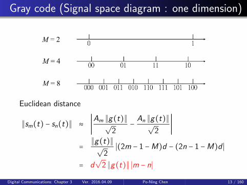
Gray code (Signal space diagram : one dimension)
Euclidean distance
∥sm(t) − sn(t)∥ ≈ ∣Am ∥g(t)∥
√2
−An ∥g(t)∥
√2
∣
=∥g(t)∥√
2∣(2m − 1 −M)d − (2n − 1 −M)d ∣
= d√
2 ∥g(t)∥ ∣m − n∣
Digital Communications: Chapter 3 Ver. 2016.04.09 Po-Ning Chen 13 / 160

Single side band (SSB) PAM
1 g(t) is real ⇔ G(f ) is Hermitian symmetric.
2 Consequently, the previous PAM is based on the DSBtransmission which requires twice the bandwidth.
3 Recall
F−1 {u−1(f )G(f )} =1
2[g(t) + ı g(t)] = g+(t)
where g(t) is the Hilbert transform of g(t).
Digital Communications: Chapter 3 Ver. 2016.04.09 Po-Ning Chen 14 / 160
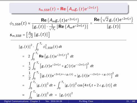
sm,SSB(t) = Re{Amg+(t)eı2πfc t}
φ1,SSB(t) ≈Re{Amg+(t)e ı2πfc t}
∥g+(t)∥ ⋅1√Ts
∥Re{Ame ı2πfc t}∥=
Re{√
2g+(t)e ı2πfc t}
∥g+(t)∥
sm,SSB = [Am√
2∥g+(t)∥]
∥g+(t)∥2⋅ ∫
Ts
0φ2
1,SSB(t)dt
= 2∫Ts
0Re{g+(t)e ı 2πfc t}
2dt
=1
2 ∫Ts
0[g+(t)e ı 2πfc t + g∗+(t)e
− ı 2πfc t]2dt
=1
2 ∫Ts
0[∣g+(t)∣e ı 2πfc t+∠g+(t) + ∣g+(t)∣e− ı 2πfc t−∠g+(t)]
2dt
= ∫
Ts
0∣g+(t)∣
2dt + ∫
Ts
0∣g+(t)∣
2cos [4πfct + 2∠g+(t)] dt
≈ ∫
Ts
0∣g+(t)∣
2dt = ∥g+(t)∥
2
Digital Communications: Chapter 3 Ver. 2016.04.09 Po-Ning Chen 15 / 160

sm,SSB(t) = Re{Am
2[g(t) ± ı g(t)] e ı2πfc t}
=Am
2g(t) cos (2πfct) ∓
Am
2g(t) sin (2πfct)
Digital Communications: Chapter 3 Ver. 2016.04.09 Po-Ning Chen 16 / 160

∥g+(t)∥2= ∥
1
2g(t) + ı
1
2g(t)∥
2
=1
2∥g(t)∥
2
Recall from Slide 2-22, x+(t) = 12(x(t) + ı x(t)) and Ex = 2Ex+ .
To summarize⎧⎪⎪⎨⎪⎪⎩
φ1(,DSB)(t) =g(t)
∥g(t)∥√
2 cos (2πfct)
sm(,DSB) = Am√2∥g(t)∥
⎧⎪⎪⎨⎪⎪⎩
φ1,SSB(t) = Re{g+(t)
∥g+(t)∥√
2e ı2πfc t}
sm,SSB = Am√2∥g+(t)∥
2-level PAM signals are particularly named antipodal signals.(±1 signals)
Digital Communications: Chapter 3 Ver. 2016.04.09 Po-Ning Chen 17 / 160

Applications of PAM
Ts = T
Digital Communications: Chapter 3 Ver. 2016.04.09 Po-Ning Chen 18 / 160

Phase-modulation (PM)
Bandpass PM
sm(t) = Re [g(t)e ı2π(m−1)/M e ı2πfc t]
= g(t) cos (2πfct + θm)
= cos (θm)g(t) cos (2πfct)´¹¹¹¹¹¹¹¹¹¹¹¹¹¹¹¹¹¹¹¹¹¹¹¹¹¹¹¹¹¹¹¹¹¹¹¹¹¹¹¹¹¸¹¹¹¹¹¹¹¹¹¹¹¹¹¹¹¹¹¹¹¹¹¹¹¹¹¹¹¹¹¹¹¹¹¹¹¹¹¹¹¹¹
φ1
− sin(θm)g(t) sin(2πfct)´¹¹¹¹¹¹¹¹¹¹¹¹¹¹¹¹¹¹¹¹¹¹¹¹¹¹¹¹¹¹¹¹¹¹¹¹¹¹¸¹¹¹¹¹¹¹¹¹¹¹¹¹¹¹¹¹¹¹¹¹¹¹¹¹¹¹¹¹¹¹¹¹¹¹¹¹¹
φ2
where θm = 2π(m − 1)/M , m = 1,2,⋯,M
Example 2 (M=4)
⎧⎪⎪⎪⎪⎪⎨⎪⎪⎪⎪⎪⎩
s1(t) = g(t) cos (2πfct)s2(t) = g(t) cos (2πfct + π/2)s3(t) = g(t) cos (2πfct + π)s4(t) = g(t) cos (2πfct + 3π/2)
Digital Communications: Chapter 3 Ver. 2016.04.09 Po-Ning Chen 19 / 160

Signal space of PM signals
⎧⎪⎪⎨⎪⎪⎩
φ1(t) ≈g(t)
∥g(t)∥√
2 cos (2πfct)
φ2(t) ≈ −g(t)
∥g(t)∥√
2 sin (2πfct)
Ô⇒
sm = [∥g(t)∥√
2cos(θm),
∥g(t)∥√
2sin(θm)]
Digital Communications: Chapter 3 Ver. 2016.04.09 Po-Ning Chen 20 / 160

Transmission energy of PM Signals
Em = ∫
T
0s2m(t)dt ≈
∥g(t)∥2
2[cos2(θm) + sin2(θm)] =
Eg
2
Advantages of PM signals : Equal energy for everychannel symbol.
Error consideration
The most possible error is the erroneous selection of anadjacent phase of the transmitted signal.
Therefore, we assign the mapping from bit pattern tochannel symbol as the adjacent signal phase differs onlyby one bit. (Gray encoding)
The most possible bit error pattern caused by the noiseis a single-bit error.
Digital Communications: Chapter 3 Ver. 2016.04.09 Po-Ning Chen 21 / 160

Signal space diagram of PM with Gray code
Digital Communications: Chapter 3 Ver. 2016.04.09 Po-Ning Chen 22 / 160

sm = [∥g(t)∥√
2cos(θm),
∥g(t)∥√
2sin(θm)]
Euclidean distance
∥sm(t) − sn(t)∥
=∥g(t)∥√
2
√
∣cos(θm) − cos(θn)∣2+ ∣sin(θm) − sin(θn)∣
2
= ∥g(t)∥√
1 − cos(θm − θn)
SSB?
Note that g(t)e ı θm is not real; hence its spectrum is notsymmetric and there is no SSB PM.
Digital Communications: Chapter 3 Ver. 2016.04.09 Po-Ning Chen 23 / 160

π/4-QPSK
A variant of 4-phase PSK (QPSK), named π/4-QPSK, isobtained by introducing an additional π/4 phase shift in thecarrier phase in each symbol interval.
Digital Communications: Chapter 3 Ver. 2016.04.09 Po-Ning Chen 24 / 160

Quadrature amplitude modulation (QAM)
Bandpass QAM
sm(t) = xi(t) cos(2πfct) − xq(t) sin(2πfct)
where xi(t) and xq(t) are quadrature components. Let
xi(t) = Amig(t) and xq(t) = Amqg(t); then bandpass QAM is
sm(t) = Amig(t) cos(2πfct) −Amqg(t) sin(2πfct)
Advantage: Transmit more digital information by using bothquadrature components as information carriers. As a result,the transfer rate of digital data is doubled.
Digital Communications: Chapter 3 Ver. 2016.04.09 Po-Ning Chen 25 / 160

Vectorization of QAM signals
sm(t) = Ami g(t) cos(2πfct)´¹¹¹¹¹¹¹¹¹¹¹¹¹¹¹¹¹¹¹¹¹¹¹¹¹¹¹¹¹¹¹¹¹¹¹¹¹¹¹¸¹¹¹¹¹¹¹¹¹¹¹¹¹¹¹¹¹¹¹¹¹¹¹¹¹¹¹¹¹¹¹¹¹¹¹¹¹¹¹
φ1
−Amq g(t) sin(2πfct)´¹¹¹¹¹¹¹¹¹¹¹¹¹¹¹¹¹¹¹¹¹¹¹¹¹¹¹¹¹¹¹¹¹¹¹¹¹¹¸¹¹¹¹¹¹¹¹¹¹¹¹¹¹¹¹¹¹¹¹¹¹¹¹¹¹¹¹¹¹¹¹¹¹¹¹¹¹
φ2
⎧⎪⎪⎨⎪⎪⎩
φ1(t) ≈g(t)
∥g(t)∥√
2 cos(2πfct)
φ2(t) ≈ −g(t)
∥g(t)∥√
2 sin(2πfct)
Ô⇒ sm = [Ami√
2∥g(t)∥ ,
Amq√
2∥g(t)∥]
Digital Communications: Chapter 3 Ver. 2016.04.09 Po-Ning Chen 26 / 160

sm = [Ami√
2∥g(t)∥ ,
Amq√
2∥g(t)∥]
Transmission energy of QAM signals
Em = ∫
T
0s2m(t)dt
=1
2∥g(t)∥
2A2mi +
1
2∥g(t)∥
2A2mq
=1
2∥g(t)∥
2(A2
mi +A2mq)
=1
2Eg (A2
mi +A2mq)
Euclidean Distance
∥sm(t) − sn(t)∥ =
√Eg
√2
√
∣Ami −Ani ∣2+ ∣Amq −Anq ∣
2
Digital Communications: Chapter 3 Ver. 2016.04.09 Po-Ning Chen 27 / 160

Signal space diagram for rectangular QAM
Digital Communications: Chapter 3 Ver. 2016.04.09 Po-Ning Chen 28 / 160

sm = [Ami√
2∥g(t)∥ ,
Amq√
2∥g(t)∥] ,
where Ami ,Amq ∈ {(2m − 1 −√M) ∶ m = 1,2,⋯,
√M}
Minimum Euclidean distance (of square QAM)
minm≠n
√Eg
2
¿ÁÁÀ∣Ami −Ani ∣
2
´¹¹¹¹¹¹¹¹¹¹¹¹¹¹¹¹¹¹¹¹¹¹¸¹¹¹¹¹¹¹¹¹¹¹¹¹¹¹¹¹¹¹¹¹¹¹¶=4
+ ∣Amq −Anq ∣2
´¹¹¹¹¹¹¹¹¹¹¹¹¹¹¹¹¹¹¹¹¹¹¹¹¹¸¹¹¹¹¹¹¹¹¹¹¹¹¹¹¹¹¹¹¹¹¹¹¹¹¹¶=0
=√
2Eg
Average symbol energy (of square QAM)
Eavg =1
M
Eg
2
√M
∑m=1
√M
∑n=1
(A2mi +A2
nq) =Eg
2M
2M(M − 1)
3=M − 1
3Eg
Average bit energy (of square QAM)
Ebavg =M − 1
3 log2 MEg
Digital Communications: Chapter 3 Ver. 2016.04.09 Po-Ning Chen 29 / 160
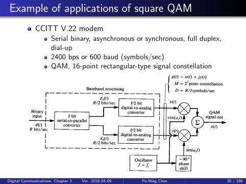
Example of applications of square QAM
CCITT V.22 modemSerial binary, asynchronous or synchronous, full duplex,dial-up2400 bps or 600 baud (symbols/sec)QAM, 16-point rectangular-type signal constellation
Digital Communications: Chapter 3 Ver. 2016.04.09 Po-Ning Chen 30 / 160

Alternative viewpoint of QAM
QAM = PM (PSK) + PAM (ASK)
Use both amplitude and phase as digital informationbearers.
sm(t) = Re [Vm1eı θm2g(t)e ı2πfc t] = Vm1g(t) cos (2πfct + θm2)
Compare with the previous viewpoint
sm(t) = Amig(t) cos(2πfct) −Amqg(t) sin(2πfct)
= Vm1g(t) cos (2πfct + θm2)
where Vm1 =√A2mi +A2
mq and θm2 = tan−1(Amq/Ami)
There is a one-to-one correspondence mapping from(Ami ,Amq) domain to (Vm1, θm2) domain.
Digital Communications: Chapter 3 Ver. 2016.04.09 Po-Ning Chen 31 / 160

Signal space for non-rectangular QAM (AM-PSK)
Digital Communications: Chapter 3 Ver. 2016.04.09 Po-Ning Chen 32 / 160
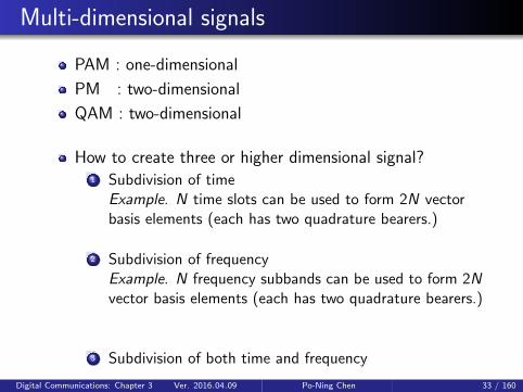
Multi-dimensional signals
PAM : one-dimensional
PM : two-dimensional
QAM : two-dimensional
How to create three or higher dimensional signal?1 Subdivision of time
Example. N time slots can be used to form 2N vectorbasis elements (each has two quadrature bearers.)
2 Subdivision of frequencyExample. N frequency subbands can be used to form 2Nvector basis elements (each has two quadrature bearers.)
3 Subdivision of both time and frequency
Digital Communications: Chapter 3 Ver. 2016.04.09 Po-Ning Chen 33 / 160

Frequency shift keying or FSK
Subdivision of frequency
Bandpass orthogonal multidimensional signals (Frequencyshift keying or FSK)
sm(t) = Re
⎡⎢⎢⎢⎢⎣
√2E
Te ı2π(m∆f )te ı2πfc t
⎤⎥⎥⎥⎥⎦
=
√2E
Tcos (2πfct + 2π(m∆f )t)
Vectorization of FSK signals under orthogonalityconditions (introduced in next few slides)
φm(t) =1
√Esm(t) and sm = [0, . . . ,0,
√E
°m-th
position
,0, . . . ,0]T
Digital Communications: Chapter 3 Ver. 2016.04.09 Po-Ning Chen 34 / 160

Crosscorrelations of FSK signals
sm,`(t) =
√2E
Te ı2π(m∆f )t and ∥sm,`(t)∥ =
√2E
ρmn,` =⟨sm,`(t), sn,`(t)⟩
∥sm,`(t)∥ ⋅ ∥sn,`(t)∥=
1
T ∫T
0e ı2π(m−n)∆f ⋅tdt
= sinc [T (m − n)∆f ] e ı πT(m−n)∆f
⟨sm(t), sn(t)⟩
∥sm(t)∥ ∥sn(t)∥= Re{ρmn,`} =
sin (πT (m − n)∆f )
πT (m − n)∆fcos (πT (m − n)∆f )
= sinc(2T (m − n)∆f )
When ∆f = k2T , Re{ρmn,`} = 0 for m ≠ n. In other words, the
minimum frequency separation between adjacent (bandpass)signals for orthogonality is ∆f = 1
2T .
Digital Communications: Chapter 3 Ver. 2016.04.09 Po-Ning Chen 35 / 160

Transmission energy of FSK signals
Em = ∫
T
0∣sm(t)∣2 dt = E
Ô⇒ Equal transmission power for each channel symbol.
Signal space diagram for FSK
Digital Communications: Chapter 3 Ver. 2016.04.09 Po-Ning Chen 36 / 160

Euclidean distance between FSK signals
Equal distance between signals
[s1 s2 ⋯ sM] =
⎡⎢⎢⎢⎢⎢⎢⎢⎢⎣
√E 0 ⋯ 0
0√E ⋯ 0
⋮ ⋮ ⋱ ⋮
0 0 ⋯√E
⎤⎥⎥⎥⎥⎥⎥⎥⎥⎦
∥sm − sn∥ =√
2E
Digital Communications: Chapter 3 Ver. 2016.04.09 Po-Ning Chen 37 / 160

Biorthogonal multidimensional FSK signals
Digital Communications: Chapter 3 Ver. 2016.04.09 Po-Ning Chen 38 / 160

Transmission energy for biorthogonal FSK signals
Em = ∫
T
0∣sm(t)∣2 dt = E
Still, equal transmission power for each channel symbol.
Cross-correlation of baseband biorthogonal FSK signals
sm,`(t) = sgn(m)
√2E
Te ı2π∣m∣(∆f ) t , m = ±1,±2,⋯,±M/2
ρmn,` =
⎧⎪⎪⎪⎨⎪⎪⎪⎩
1, m = n−1, m = −n
0, otherwise
Digital Communications: Chapter 3 Ver. 2016.04.09 Po-Ning Chen 39 / 160

Euclidean distance between signals
[s−1 ⋯ s−M/2 s1 ⋯ sM/2]
=
⎡⎢⎢⎢⎢⎢⎢⎢⎢⎣
−√E 0 ⋯ 0
√E 0 ⋯ 0
0 −√E ⋯ 0 0
√E ⋯ 0
⋮ ⋮ ⋱ ⋮ ⋮ ⋮ ⋱ ⋮
0 0 ⋯ −√E 0 0 ⋯
√E
⎤⎥⎥⎥⎥⎥⎥⎥⎥⎦
Hence
∥sm − sn∥ =⎧⎪⎪⎨⎪⎪⎩
√2E if m ≠ −n
2√E if m = −n
Digital Communications: Chapter 3 Ver. 2016.04.09 Po-Ning Chen 40 / 160

Simplex signals
Given the vector representations of orthogonal andequal-power channel symbols (such as FSK)
sm = [am1, am2, ⋯ , amk]
for m = 1,2,⋯,M , its center (of gravity under equal priorprobability assumption) is
c = [1
M
M
∑m=1
am1,1
M
M
∑m=1
am2, ⋯,1
M
M
∑m=1
amk]
Define new channel symbol as
s ′m = sm − c
Then {s ′1, s ′2,⋯, s ′M} is called the simplex signal.
Digital Communications: Chapter 3 Ver. 2016.04.09 Po-Ning Chen 41 / 160
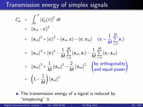
Transmission energy of simplex signals
E ′m = ∫
T
0∣s ′m(t)∣2 dt
= ∥sm − c∥2
= ∥sm∥2+ ∥c∥2
− ⟨sm,c⟩ − ⟨c , sm⟩ (c =1
M
M
∑i=1
s i)
= ∥sm∥2+ ∥c∥2
−1
M
M
∑i=1
⟨sm, s i⟩ −1
M
M
∑i=1
⟨s i , sm⟩
= ∥sm∥2+
1
M∥sm∥
2−
2
M∥sm∥
2(
by orthogonalityand equal-power
)
= (1 −1
M) ∥sm∥
2
The transmission energy of a signal is reduced by“simplexing” it.
Digital Communications: Chapter 3 Ver. 2016.04.09 Po-Ning Chen 42 / 160

Crosscorrelation of simplex signals
ρmn =⟨s ′m, s ′n⟩∥s ′m∥ ∥s ′n∥
=⟨sm − c , sn − c⟩(1 − 1
M) ∥sm∥
2
=⟨sm, sn⟩ − ⟨sm,c⟩ − ⟨c , sn⟩ + ⟨c ,c⟩
(1 − 1M) ∥sm∥
2
=
⎧⎪⎪⎪⎪⎨⎪⎪⎪⎪⎩
∥sm∥2− 2M
∥sm∥2+ 1M
∥sm∥2
(1− 1M
)∥sm∥2 m = n
0 − 2M
∥sm∥2+ 1M
∥sm∥2
(1− 1M
)∥sm∥2 m ≠ n
= {1 m = n
− 1M−1 m ≠ n
Simplex signals are equally correlated !
Digital Communications: Chapter 3 Ver. 2016.04.09 Po-Ning Chen 43 / 160
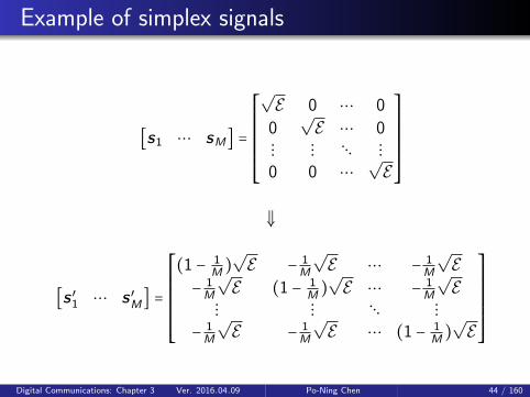
Example of simplex signals
[s1 ⋯ sM] =
⎡⎢⎢⎢⎢⎢⎢⎢⎢⎣
√E 0 ⋯ 0
0√E ⋯ 0
⋮ ⋮ ⋱ ⋮
0 0 ⋯√E
⎤⎥⎥⎥⎥⎥⎥⎥⎥⎦
⇓
[s ′1 ⋯ s ′M] =
⎡⎢⎢⎢⎢⎢⎢⎢⎢⎣
(1 − 1M )
√E − 1
M
√E ⋯ − 1
M
√E
− 1M
√E (1 − 1
M )√E ⋯ − 1
M
√E
⋮ ⋮ ⋱ ⋮
− 1M
√E − 1
M
√E ⋯ (1 − 1
M )√E
⎤⎥⎥⎥⎥⎥⎥⎥⎥⎦
Digital Communications: Chapter 3 Ver. 2016.04.09 Po-Ning Chen 44 / 160

Subdivision of time: N time slots
For example: BPSK in each dimension
sm = [cm,0, cm,1,⋯, cm,N−1] , 1 ≤ m ≤M
where NTc = T
“cm,j = 0” ≡ “g1(t) is transmitted at time slot j”
“cm,j = 1” ≡ “g2(t) is transmitted at time slot j”
g1(t) = +
√2EcTc
cos(2πfct), g2(t) = −
√2E
Tcos(2πfct),
with t ∈ [0,Tc)
sm(t) =
√2EcTc
N−1
∑j=0
(−1)cm,j cos (2πfc(t − jTc))1{jTc ≤ t < (j+1)Tc}
Digital Communications: Chapter 3 Ver. 2016.04.09 Po-Ning Chen 45 / 160

Crosscorrelation coefficient of adjacent signals(i.e., with only one distinct component)
For those identical components
∫
Tc
0∣g1(t)∣
2 dt = ∫Tc
0∣g2(t)∣
2 dt = Ec
For the single distinct component
∫
Tc
0g1(t)g
∗2 (t)dt = ∫
Tc
0−∣g1(t)∣
2 dt = −Ec
Hence
ρmn =⟨sm, sn⟩
∥sm∥ ∥sn∥=
(N − 1)Ec − EcNEc
= 1 −2
N
Minimum Euclidean distance between adjacent codewords
minm≠n
∥sm − sn∥ = minm≠n
√
∥sm∥2+ ∥sn∥
2− ⟨sm, sn⟩ − ⟨sn, sm⟩
=
√
NEc +NEc − 2(NEc)N − 2
N= 2
√Ec
Digital Communications: Chapter 3 Ver. 2016.04.09 Po-Ning Chen 46 / 160

Transmission energy of multidimensional BPSK signals
Em = ∫
T
0∣sm(t)∣
2dt = N ∥g1(t)∥
2= N ∫
Tc
0∣g1(t)∣
2 dt = NEc
Largest number of channel symbols
M ≤ 2N
Vectorization of BPSK signals
sm =
⎡⎢⎢⎢⎢⎢⎢⎢⎣
±√Ec
±√Ec⋮
±√Ec
⎤⎥⎥⎥⎥⎥⎥⎥⎦N×1
Can we properly choose {sm}Mm=1 such that they areorthogonal to each other ?
Digital Communications: Chapter 3 Ver. 2016.04.09 Po-Ning Chen 47 / 160

Orthogonal multidimensional signals: Hadamard
signals
Definition: The Hadamard signals of size M = 2n can berecursively defined as
Hn = [Hn−1 Hn−1
Hn−1 −Hn−1]
with initial value H0 = [1].For example,
H1 = [1 11 -1
] and H2 =
⎡⎢⎢⎢⎢⎢⎢⎢⎣
1 1 1 11 -1 1 -11 1 -1 -11 -1 -1 1
⎤⎥⎥⎥⎥⎥⎥⎥⎦
Digital Communications: Chapter 3 Ver. 2016.04.09 Po-Ning Chen 48 / 160

Hence, when M = 4, the Hadamard multidimensionalorthogonal (BPSK) signals are
[s1 s2 s3 s4] =
⎡⎢⎢⎢⎢⎢⎢⎢⎣
√Ec
√Ec
√Ec
√Ec√
Ec −√Ec
√Ec −
√Ec√
Ec√Ec −
√Ec −
√Ec√
Ec −√Ec −
√Ec
√Ec
⎤⎥⎥⎥⎥⎥⎥⎥⎦
Digital Communications: Chapter 3 Ver. 2016.04.09 Po-Ning Chen 49 / 160

3.3 Signaling schemes with memory
Digital Communications: Chapter 3 Ver. 2016.04.09 Po-Ning Chen 50 / 160

Memoryless modulation: smi(t), mi ∈ {1,2, . . . ,M},
mi =function of Blocki
Modulation with memory: smi(t),
mi =function of (Blocki , Blocki−1,⋯, Blocki−(L−1))
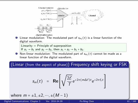
Linear modulation: The modulated part of smi(t) is a
linear function of the digital waveform.Linearity = Principle of superposition
If a1 → b1 and a2 → b2, then a1 + a2 → b1 + b2.
Non-linear modulation:Digital Communications: Chapter 3 Ver. 2016.04.09 Po-Ning Chen 51 / 160

Why introducing “memory” into signals?
The signal dependence is introduced for the purpose ofshaping the spectrum of transmitted signal so that itmatches the spectral characteristics of the channel.
Linearity
For example, smi (t) = Re{Ami e2πfc t}.
⎧⎪⎪⎪⎪⎪⎪⎪⎨⎪⎪⎪⎪⎪⎪⎪⎩
−3 Ð→ Re{−3e2πfc t}
−1 Ð→ Re{−1e2πfc t}
+1 Ð→ Re{+1e2πfc t}
+3 Ð→ Re{+3e2πfc t}
So, if the modulated part of smi (t) cannot be made as alinear function of the digital waveform, the modulation isclassified as non-linear.
Digital Communications: Chapter 3 Ver. 2016.04.09 Po-Ning Chen 52 / 160

Digital Communications: Chapter 3 Ver. 2016.04.09 Po-Ning Chen 53 / 160

Linear modulations with/without memory
NRZ (Non-Return-to-Zero) =Binary PAM or binary PSK: memoryless
channel code bit = input bit
NRZI (Non-Return-to-Zero, Inverted) =Differentialencoding : with memory
(channel code bit)k = (input bit)k ⊕ (channel code bit)k−1
⎧⎪⎪⎪⎪⎨⎪⎪⎪⎪⎩
(channel code bit)k = (channel code bit)k−1, when (input bit)k = 0
(channel code bit)k = (channel code bit)k−1, when (input bit)k = 1
Digital Communications: Chapter 3 Ver. 2016.04.09 Po-Ning Chen 54 / 160

Application: DBPSK/DQPSK in Wireless LAN
Digital Communications: Chapter 3 Ver. 2016.04.09 Po-Ning Chen 55 / 160
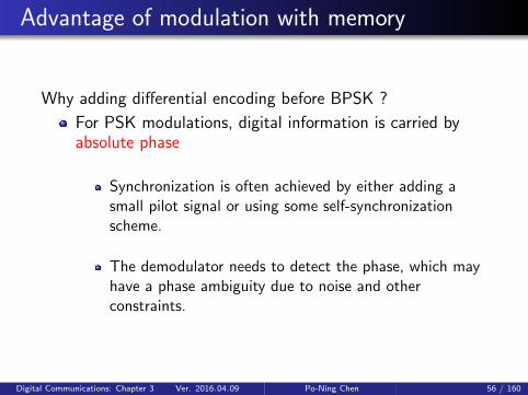
Advantage of modulation with memory
Why adding differential encoding before BPSK ?
For PSK modulations, digital information is carried byabsolute phase
Synchronization is often achieved by either adding asmall pilot signal or using some self-synchronizationscheme.
The demodulator needs to detect the phase, which mayhave a phase ambiguity due to noise and otherconstraints.
Digital Communications: Chapter 3 Ver. 2016.04.09 Po-Ning Chen 56 / 160

Example of phase ambiguity (frequency shift)
Ideal (noiseless) case
{ftransmiter = fc ∶ receive cos (2πfct + θ)freceiver = fc ∶ estimate it based on fc
Ô⇒ estimate θ = θ
Ambiguous case
{ftransmiter = fc ∶ receive cos (2πfct + θ)freceiver ≠ fc ∶ estimate it based on f ′c
Ô⇒ {receive cos (2πf ′c t + [2π(fc − f ′c )t] + θ)estimate it based on f ′c
Ô⇒ estimate θ = [2π(fc − f ′c )t] + θ
Digital Communications: Chapter 3 Ver. 2016.04.09 Po-Ning Chen 57 / 160

Advantage of differential encoding
(channel code bit)k = (input bit)k ⊕ (channel code bit)k−1
The phases or signs of the received waveforms are notimportant for detection.
What is important is the change in the sign of successivepulses.
The sign change can be detected even if thedemodulating carrier has a phase ambiguity.
Digital Communications: Chapter 3 Ver. 2016.04.09 Po-Ning Chen 58 / 160

Advantage of diff encode (Noncoherent demod.)
No need to generate a local carrier (at the receiver side).
Use the received signal itself as a carrier.
±A cos(2πfct) -
? DelayT0
6⊗ - Lowpass
fileter-
z(t)y(t)
y(t −T0)
z(t) =
⎧⎪⎪⎪⎪⎪⎪⎪⎪⎪⎨⎪⎪⎪⎪⎪⎪⎪⎪⎪⎩
A2c cos2(2πfct) =
A2c
2 + 12 cos (4πfct)→
12A
2c ,
if y(t) = y(t −T0)
−A2c cos2(2πfct) = −
A2c
2 − 12 cos (4πfct)→ −1
2A2c ,
if y(t) = −y(t −T0)
Digital Communications: Chapter 3 Ver. 2016.04.09 Po-Ning Chen 59 / 160

Nonlinear modulation methods withmemory
Digital Communications: Chapter 3 Ver. 2016.04.09 Po-Ning Chen 60 / 160
Linear modulation: The modulated part of smi (t) is a linear function of thedigital waveform.
Linearity = Principle of superpositionIf a1 → b1 and a2 → b2, then a1 + a2 → b1 + b2.
Non-linear modulation: The modulated part of smi (t) cannot be made as alinear function of the digital waveform.
(Linear (from the aspect of phase)) Frequency shift keying or FSK
sm(t) = Re
⎡⎢⎢⎢⎢⎣
√2E
Te ı2π(m∆f )te ı2πfc t
⎤⎥⎥⎥⎥⎦
where m = ±1,±2,⋯,±(M − 1)Digital Communications: Chapter 3 Ver. 2016.04.09 Po-Ning Chen 61 / 160

Motivation: Disadvantages of FSK
Potential obstacles of multidimensional FSK with (M − 1)oscillators for each desired frequency
Abrupt switching from one oscillator to another willresult in relatively large spectral side lobes outside of themain spectral band of the signal.
Continuous-Phase FSK (CPFSK)
Alternative implementation of multidimensional FSK
A single carrier whose frequency is changed continuously.
This is considered as a modulated signal with memory(we will explain this point in the next few slides).
Digital Communications: Chapter 3 Ver. 2016.04.09 Po-Ning Chen 62 / 160

Recall
s(t) = Re{s`(t)eı2πfc t} , s`(t) = xi(t) + ı xq(t)
s`(t) is the baseband version of the bandpass signal s(t).
For ideal FSK signals
sm(t) = Re
⎡⎢⎢⎢⎢⎣
√2E
Te ı2π(m∆f )te ı2πfc t
⎤⎥⎥⎥⎥⎦
Ô⇒ sm,`(t) =
√2E
Te ı2π(m∆f )t
where ∆f = fd and m = ±1,±2,⋯,±(M − 1).
Digital Communications: Chapter 3 Ver. 2016.04.09 Po-Ning Chen 63 / 160

Example of ideal (2-OSC) FSK signals
Let T = 0.5 sec, E = 0.25, fd = 0.5, In (= m) ∈ {1,−1}, andfc = 1.5 Hz.
s(t) = Re{s`(t)eı2πfc t} = {
cos(4πt) In = 1cos(2πt), In = −1
Digital Communications: Chapter 3 Ver. 2016.04.09 Po-Ning Chen 64 / 160

Discontinuous phase of (2-OSC) FSK
Phase of s`(t) = {πt, In = 1−πt, In = −1
for t ∈ [nT , (n + 1)T )
Digital Communications: Chapter 3 Ver. 2016.04.09 Po-Ning Chen 65 / 160

Phase change of (2-OSC) FSK
(Normalized) phase change (for t ∈ [nT , (n + 1)T ))
d(t) =phase of s`(t)
4πTfd=
∂∂t (2πInfdt)
4πTfd=
In2T
is the derivative of the phase!
Continue from the previous example with T = 0.5.
d(t) = (+1)[u−1(t) − u−1(t −T)] − δ(t −T)+ (−1)[u−1(t −T) − u−1(t − 2T)]+ (−1)[u−1(t − 2T) − u−1(t − 3T)] + 3δ(t − 3T)+ (+1)[u−1(t − 3T) − u−1(t − 4T)] +⋯
Digital Communications: Chapter 3 Ver. 2016.04.09 Po-Ning Chen 66 / 160

d(t)= I0 [u−1(t ) − u−1(t −T )] + 1{I0 ≠ I1} ⋅ I1 ⋅ 1 ⋅ δ(t −T )
+ I1 [u−1(t −T ) − u−1(t − 2T )] + 1{I1 ≠ I2} ⋅ I2 ⋅ 2 ⋅ δ(t − 2T )
+ I2 [u−1(t − 2T ) − u−1(t − 3T )] + 1{I2 ≠ I3} ⋅ I3 ⋅ 3 ⋅ δ(t − 3T )
+ I3 [u−1(t − 3T ) − u−1(t − 4T )] + 1{I3 ≠ I4} ⋅ I4 ⋅ 4 ⋅ δ(t − 4T )
+⋯
Phase change is the derivative of the phase!
Phase is the integration of phase change!
s`(t) =
√2E
Te ı4πTfd ∫ t
−∞ d(τ)dτ
Those δ(⋅) functions result in “discontinuity” inintegration! Hence, let us remove them to force“continuity” in phase.
Digital Communications: Chapter 3 Ver. 2016.04.09 Po-Ning Chen 67 / 160
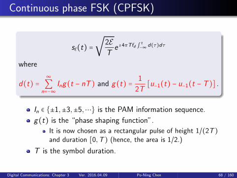
Continuous phase FSK (CPFSK)
s`(t) =
√2E
Te ı4πTfd ∫ t
−∞ d(τ)dτ
where
d(t) =∞∑
n=−∞Ing(t − nT ) and g(t) =
1
2T[u−1(t) − u−1(t −T )] .
In ∈ {±1,±3,±5,⋯} is the PAM information sequence.
g(t) is the “phase shaping function”.
It is now chosen as a rectangular pulse of height 1/(2T )
and duration [0,T ) (hence, the area is 1/2.)
T is the symbol duration.
Digital Communications: Chapter 3 Ver. 2016.04.09 Po-Ning Chen 68 / 160
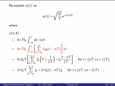
Re-express s`(t) as
s`(t) =
√2E
Te ı φ(t;I)
where
φ(t; I)
= 4πTfd ∫t
−∞d(τ)dτ
= 4πTfd ∫t
−∞[
∞∑
n=−∞Ing(τ − nT )] dτ
= 4πfdT [n−1
∑k=−∞
Ik (T ×1
2T) + In
t − nT
2T] for t ∈ [nT , (n + 1)T )
= 2πfdTn−1
∑k=−∞
Ik + 2πfd(t − nT )In for t ∈ [nT , (n + 1)T )
Digital Communications: Chapter 3 Ver. 2016.04.09 Po-Ning Chen 69 / 160

(Cont.)For t ∈ [nT , (n + 1)T ), s`(t) =√
2ET e ı φ(t;I) with
φ(t; I ) = 2πfdTn−1
∑k=−∞
Ik + 2πfd(t − nT )In
= θn + 2πh ⋅ In ⋅ q(t − nT ),
where
⎧⎪⎪⎪⎪⎪⎪⎪⎪⎪⎪⎪⎪⎨⎪⎪⎪⎪⎪⎪⎪⎪⎪⎪⎪⎪⎩
h = 2fdT (modulation index)
θn = πhn−1
∑k=−∞
Ik (accumulation of history/memory)
q(t) =
⎧⎪⎪⎪⎪⎨⎪⎪⎪⎪⎩
0 t < 0t
2T 0 ≤ t < T12 t ≥ T
(integration of g(t))
Digital Communications: Chapter 3 Ver. 2016.04.09 Po-Ning Chen 70 / 160

Generalization of CPFSK: CPM
We can further generalize φ(t; I ) to
φ(t; I ) = 2πn
∑k=−∞
hk ⋅ Ik ⋅ q(t − kT )
for nT ≤ t < (n + 1)T
where
1 I = {Ik}∞k=−∞ is the sequence of PAM symbols in{±1,±3, . . . ,±(M − 1)}.
2 hk is the modulation index.If hk varies with k , it is called multi-h CPM.
3 q(t) = ∫t
0 g(τ)dτ.If g(t) = 0 for t ≥ T (and t < 0), s`(t) is called full-response CPM;otherwise it is called partial-response CPM.
Digital Communications: Chapter 3 Ver. 2016.04.09 Po-Ning Chen 71 / 160

Examples of CPMs
Digital Communications: Chapter 3 Ver. 2016.04.09 Po-Ning Chen 72 / 160

Examples of CPMs
Digital Communications: Chapter 3 Ver. 2016.04.09 Po-Ning Chen 73 / 160

Some commonly used CPM pulse shapes
LREC (Rectangular): LREC with L = 1 is CPFSK
g(t) =1
2LT(u−1(t) − u−1(t − LT ))
LRC (Raised cosine)
g(t) =1
2LT(u−1(t) − u−1(t − LT )) (1 − cos(
2πt
LT))
Digital Communications: Chapter 3 Ver. 2016.04.09 Po-Ning Chen 74 / 160

Some commonly used CPM pulse shapes
GMSK (Gaussian minimum shift keying)
g(t) = Q (2πB (t −T
2) /
√ln 2)−Q (2πB (t +
T
2) /
√ln 2)
where Q(t) = ∫∞t
1√2πe−x
2/2 dx , and B is 3dB Bandwidth
g(t) is the response of filter H(f ) = e−ln(2)
2( fB)2
to arectangular pulse of u−1(t +T /2) − u−1(t −T /2).
GMSK with BT = 0.3 is used in the European digitalcellular communication system, called GSM (2G).
At BT = 0.3, the GMSK pulse may be truncated at∣t ∣ = 1.5T with a relatively small error incurred fort > 1.5T .
Digital Communications: Chapter 3 Ver. 2016.04.09 Po-Ning Chen 75 / 160

Representations of continuous-phase
Phase trajectory or phase tree
Phase trellis
Digital Communications: Chapter 3 Ver. 2016.04.09 Po-Ning Chen 76 / 160

Phase trajectory or phase tree
Binary CPFSK (i.e., In = ±1 and g(t) is full responserectangular function)
φ (t; I ) = πhn−1
∑k=−∞
Ik + 2πhIn ⋅ q(t − nT )
Digital Communications: Chapter 3 Ver. 2016.04.09 Po-Ning Chen 77 / 160

Example 3
Quaternary CPFSK (See the next page) withIn ∈ {−3,−1,+1,+3}.
We observe that the phase trees for CPFSK are piecewiselinear as a consequence of the fact that the pulse g(t) isrectangular.
Smoother phase trajectories and phase trees are obtainedby using pulses that do not contain discontinuities.
Digital Communications: Chapter 3 Ver. 2016.04.09 Po-Ning Chen 78 / 160

Digital Communications: Chapter 3 Ver. 2016.04.09 Po-Ning Chen 79 / 160

If g(t) is continuous (especially at boundaries), phasetrajectory becomes smooth.
Example 4
g(t) =1
6T(1 − cos(
2πt
3T)) = raised cosine of length 3T
with (I−2, I−1, I0, I1, I2,⋯) = (+1,+1,+1,−1,−1,−1,+1,+1,−1,+1,⋯)
Digital Communications: Chapter 3 Ver. 2016.04.09 Po-Ning Chen 80 / 160

Phase trellis
Phase trellis = Phase trajectory is plotted with modulo 2π
Example 5
Binary CPFSK with h = 1/2 and g(t) is a full responserectangular function.
Thus CPM can be decoded by Viterbi trellis decoding.Digital Communications: Chapter 3 Ver. 2016.04.09 Po-Ning Chen 81 / 160

Minimum shift keying (MSK)
Recall for nT ≤ t < (n + 1)T , CPM has
φ(t; I ) = 2πn
∑k=−∞
hk ⋅ Ik ⋅ q(t − kT ).
CPFSK is a special case of CPM with
g(t) = 12T for 0 ≤ t < T
MSK is a special case of binary CPFSK with
hk =12 , g(t) = 1
2T for 0 ≤ t < T and In ∈ {±1}
Thus for MSK, we have for nT ≤ t < (n + 1)T ,
φ(t; I ) =π
2
n−1
∑k=−∞
Ik + πInq(t − nT ) = θn +1
2πIn (
t − nT
T)
Digital Communications: Chapter 3 Ver. 2016.04.09 Po-Ning Chen 82 / 160

Φ(t; I ) = θn +1
2πIn (
t − nT
T) = 2π (
In4T
) t −nπIn
2+ θn
The corresponding modulated carrier wave is
sMSK(t) = A cos (2πfct +Φ(t; I ))
= A cos [2π (fc +In
4T) t −
nπIn2
+ θn]
Since In ∈ {±1}, sMSK(t) has two frequency components:
f1 = fc −1
4T
f2 = fc +1
4T
Digital Communications: Chapter 3 Ver. 2016.04.09 Po-Ning Chen 83 / 160
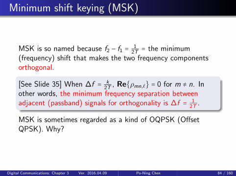
Minimum shift keying (MSK)
MSK is so named because f2 − f1 =1
2T = the minimum(frequency) shift that makes the two frequency componentsorthogonal.
[See Slide 35] When ∆f = k2T , Re{ρmn,`} = 0 for m ≠ n. In
other words, the minimum frequency separation betweenadjacent (passband) signals for orthogonality is ∆f = 1
2T .
MSK is sometimes regarded as a kind of OQPSK (OffsetQPSK). Why?
Digital Communications: Chapter 3 Ver. 2016.04.09 Po-Ning Chen 84 / 160

Offset QPSK
The original QPSK
There could be 180 degree of (sudden) phase change (so, notcontinuous phase), e.g., from (+1,+1) to (−1,−1).
Digital Communications: Chapter 3 Ver. 2016.04.09 Po-Ning Chen 85 / 160

sQPSK(t) =∞∑
n=−∞I2ng(t − 2nT ) cos(2πfc)
−∞∑
n=−∞I2n+1g(t − 2nT ) sin (2πfct)
(I0, I1) = (+1,+1), (I2, I3) = (−1,−1) and (I4, I5) = (−1,+1).g(t) rectangular pulse of unit height and during 2T .
Digital Communications: Chapter 3 Ver. 2016.04.09 Po-Ning Chen 86 / 160

Offset QPSK (OQPSK)
How to reduce the 180o phase change to only 90o?
Simple solution: Do not let the “two bits” I2n and I2n+1 changeat the same time!
0 2T 4T 6T
T 3T 5T 7T
I0 = 1 I2 = −1 I4 = −1
I1 = 1 I3 = −1 I5 = −1
sOQPSK(t) =∞∑
n=−∞I2ng(t − 2nT ) cos(2πfct)
−∞∑
n=−∞I2n+1g(t − (2n + 1)T ) sin (2πfct)
Digital Communications: Chapter 3 Ver. 2016.04.09 Po-Ning Chen 87 / 160

To synchronize with the textbook, we reverse {I2n+1} to obtain
sOQPSK(t) =∞∑
n=−∞I2ng(t − 2nT ) cos(2πfct)
+∞∑
n=−∞I2n+1g(t − (2n + 1)T ) sin (2πfct)
Digital Communications: Chapter 3 Ver. 2016.04.09 Po-Ning Chen 88 / 160

OQPSK vs. MSK
MSK can be regarded as a kind of (memoryless) OQPSK.Why?
Proof: Suppose without loss of generality,
θ0 =π
2
−1
∑k=−∞
Ik =3π
2.
Then for nT ≤ t < (n + 1)T ,
sMSK,`(t) = e ı φ(t;I)
= e ı2π( In4T
)t⋅ e− ı
nπ2In ⋅ e ı
π2 ∑
n−1k=0 Ik ⋅ e ı θ0
= [cos(πt
2T) + ı In sin(π
t
2T)] (−In ı )
n(n−1
∏k=0
(Ik ı )) (− ı )
= I n+1n (
n−1
∏k=0
Ik) sin(πt
2T) + ı I nn (
n−1
∏k=0
Ik) sin(π(t −T )
2T)
Digital Communications: Chapter 3 Ver. 2016.04.09 Po-Ning Chen 89 / 160

n I n+1n (∏
n−1k=0 Ik) I nn (∏
n−1k=0 Ik)
0 J0 = I0 = J2⌊0/2⌋1 J0 = I0 = J2⌊1/2⌋ J1 = I0I1 = J2⌊(1−1)/2⌋+1
2 J2 = I0I1I2 = J2⌊2/2⌋ J1 = I0I1 = J2⌊(2−1)/2⌋+1
3 J2 = I0I1I2 = J2⌊3/2⌋ J3 = I0I1I2I3 = J2⌊(3−1)/2⌋+1
4 J4 = I0I1I2I3I4 = J2⌊4/2⌋ J3 = I0I1I2I3 = J2⌊(4−1)/2⌋+1
5 J4 = I0I1I2I3I4 = J2⌊5/2⌋ J5 = I0I1I2I3I4I5 = J2⌊(5−1)/2⌋+1
6 J6 = I0I1I2I3I4I5I6 = J2⌊6/2⌋ J5 = I0I1I2I3I4I5 = J2⌊(6−1)/2⌋+1
For nT ≤ t < (n + 1)T ,
sMSK,`(t) = J2⌊n/2⌋(−1)⌊n/2⌋ sin(π(t − 2⌊n/2⌋T )
2T)
´¹¹¹¹¹¹¹¹¹¹¹¹¹¹¹¹¹¹¹¹¹¹¹¹¹¹¹¹¹¹¹¹¹¹¹¹¹¹¹¹¹¹¹¹¹¹¹¹¹¹¹¹¹¹¹¹¹¹¹¹¹¸¹¹¹¹¹¹¹¹¹¹¹¹¹¹¹¹¹¹¹¹¹¹¹¹¹¹¹¹¹¹¹¹¹¹¹¹¹¹¹¹¹¹¹¹¹¹¹¹¹¹¹¹¹¹¹¹¹¹¹¹¹¶g(t−2⌊n/2⌋T)
− ı J2⌊(n−1)/2⌋+1(−1)⌊(n−1)/2⌋+1 sin(π(t − 2⌊(n − 1)/2⌋T −T )
2T)
´¹¹¹¹¹¹¹¹¹¹¹¹¹¹¹¹¹¹¹¹¹¹¹¹¹¹¹¹¹¹¹¹¹¹¹¹¹¹¹¹¹¹¹¹¹¹¹¹¹¹¹¹¹¹¹¹¹¹¹¹¹¹¹¹¹¹¹¹¹¹¹¹¹¹¹¹¹¹¹¹¹¹¹¹¹¹¹¹¹¹¹¹¹¹¹¹¹¹¹¸¹¹¹¹¹¹¹¹¹¹¹¹¹¹¹¹¹¹¹¹¹¹¹¹¹¹¹¹¹¹¹¹¹¹¹¹¹¹¹¹¹¹¹¹¹¹¹¹¹¹¹¹¹¹¹¹¹¹¹¹¹¹¹¹¹¹¹¹¹¹¹¹¹¹¹¹¹¹¹¹¹¹¹¹¹¹¹¹¹¹¹¹¹¹¹¹¹¹¹¶g(t−2⌊(n−1)/2⌋T−T)
Digital Communications: Chapter 3 Ver. 2016.04.09 Po-Ning Chen 90 / 160
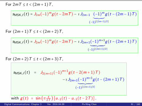
For 2mT ≤ t < (2m + 1)T ,
sMSK,`(t) = J2m(−1)mg(t − 2mT ) − ı J2m−1 (−1)m
´¹¹¹¹¸¹¹¹¹¹¶(−1)⌈(2m−1)/2⌉
g(t − (2m − 1)T )
For (2m + 1)T ≤ t < (2m + 2)T ,
sMSK,`(t) = J2m(−1)mg(t − 2mT ) − ı J2m+1(−1)m+1
´¹¹¹¹¹¹¹¹¹¹¹¹¸¹¹¹¹¹¹¹¹¹¹¹¹¹¶(−1)⌈(2m+1)/2⌉
g(t − (2m + 1)T )
For (2m + 2)T ≤ t < (2m + 3)T ,
sMSK,`(t) = J2(m+1)(−1)m+1g(t − 2(m + 1)T )
− ı J2m+1(−1)m+1
´¹¹¹¹¹¹¹¹¹¹¹¹¸¹¹¹¹¹¹¹¹¹¹¹¹¹¶(−1)⌈(2m+1)/2⌉
g(t − (2m + 1)T )
with g(t) = sin (π t2T
) [u−1(t) − u−1(t − 2T )] .
Digital Communications: Chapter 3 Ver. 2016.04.09 Po-Ning Chen 91 / 160

MSK can be regarded as a memoryless OQPSK by setting
sMSK(t) = [∞∑
n=−∞I2ng(t − 2nT )] cos(2πfct)
+ [∞∑
n=−∞I2n+1g(t − (2n + 1)T )] sin (2πfct)
with
In = (−1)⌈n/2⌉Jn = (−1)⌈n/2⌉n
∏k=0
Ik .
MSK can be “composed” using “memoryless” circuitswith “with-memory” information sequence I .
Please be noted that the textbook abuses the notation byusing g(t) to denote both the amplitude and phase pulseshaping functions for CPM signals!
Digital Communications: Chapter 3 Ver. 2016.04.09 Po-Ning Chen 92 / 160

A linear representation of CPM
The key of OQPSK representation of MSK is that phase canbe “pulled down” as a multiplicative adjustment in amplitudewhen In ∈ {−1,+1}!
For example, e ı2π( In4T
)t= cos(π
t
2T) + ı In sin(π
t
2T)
(1986 Laurent)
CPM can also be represented as a linear superposition ofAM signal waveforms (if In ∈ {±1}).
Such a representation provides an alternative method forgenerating CPM signal at the transmitter and fordemodulating the signal at the receiver.
Digital Communications: Chapter 3 Ver. 2016.04.09 Po-Ning Chen 93 / 160

An important and useful fact
For I ∈ {−1,+1},
e ıA⋅I =sin(B −A)
sin(B)+ e ıB ⋅I
sin(A)
sin(B).
Proof:
sin(B)e ıA⋅I
= sin(B)[cos(A) + ı I sin(A)]
= sin(B) cos(A) + ı sin(B ⋅ I ) sin(A)
= sin(B −A) + cos(B) sin(A) + ı sin(B ⋅ I ) sin(A)
= sin(B −A) + sin(A)[cos(B ⋅ I ) + ı sin(B ⋅ I )]
= sin(B −A) + sin(A)e ıB ⋅I
◻
Digital Communications: Chapter 3 Ver. 2016.04.09 Po-Ning Chen 94 / 160

For general h and g(⋅) function of duration L and of integral1/2 (but each In ∈ {±1}), we have for nT ≤ t < (n + 1)T (for abinary CPM signal),
sb-CPM,`(t) = e ı φ(t;I)
= e ı (πh∑n−Lk=−∞ Ik+2πh∑n
k=n−L+1 Ikq(t−kT))
= e ı πh∑n−Lk=−∞ Ik
L−1
∏k ′=0
e ı2πhIn−k′q(t−(n−k ′)T) (n − k ′ = k)
= e ı πh∑n−Lk=−∞ Ik
L−1
∏k ′=0
(sin(B − 2πh q(t − (n − k ′)T ))
sin(B)
+e ıB ⋅In−k′sin(2πh q(t − (n − k ′)T ))
sin(B)) ,
where B = πh.
Digital Communications: Chapter 3 Ver. 2016.04.09 Po-Ning Chen 95 / 160

Define
s0(t) =
⎧⎪⎪⎪⎪⎪⎨⎪⎪⎪⎪⎪⎩
sin(2πh q(t))sin(B) 0 ≤ t < LT
sin(B−2πh q(t−LT))sin(B) LT ≤ t < 2LT
0 otherwise
Since q(0) = 0 and q(LT ) = 1/2, s0(t) is continuous for t ∈ R.
Digital Communications: Chapter 3 Ver. 2016.04.09 Po-Ning Chen 96 / 160

Continue the derivation:
sb-CPM,`(t)
= e ı πh∑n−Lk=−∞ Ik
L−1
∏k ′=0
(sin(B − 2πhq(t − (n − k ′)T + LT − LT ))
sin(B)
+e ıB ⋅In−k′sin(2πhq(t − (n − k ′)T ))
sin(B))
= e ı πh∑n−Lk=−∞ Ik
L−1
∏k ′=0
(s0(t − (n − k ′)T + LT )
+e ıB ⋅In−k′ s0(t − (n − k ′)T ))
nT ≤ t < (n + 1)T and 0 ≤ k ′ ≤ L − 1 imply that
0 ≤ t − (n − k ′)T < LT and LT ≤ t − (n − k ′)T + LT < 2LT .
Digital Communications: Chapter 3 Ver. 2016.04.09 Po-Ning Chen 97 / 160

L−1
∏k ′=0
(s0(t − (n − k ′)T + LT ) + e ıB ⋅In−k′ s0(t − (n − k ′)T ))
= ( s0(t − nT + 0 ⋅T + LT )´¹¹¹¹¹¹¹¹¹¹¹¹¹¹¹¹¹¹¹¹¹¹¹¹¹¹¹¹¹¹¹¹¹¹¹¹¹¹¹¹¹¹¹¹¹¹¹¹¹¹¹¹¹¹¹¹¹¹¹¹¹¹¹¹¹¹¹¸¹¹¹¹¹¹¹¹¹¹¹¹¹¹¹¹¹¹¹¹¹¹¹¹¹¹¹¹¹¹¹¹¹¹¹¹¹¹¹¹¹¹¹¹¹¹¹¹¹¹¹¹¹¹¹¹¹¹¹¹¹¹¹¹¹¹¹¹
ai,0=1 (k ′=0)
+e ıB ⋅In−0 s0(t − nT + 0 ⋅T )´¹¹¹¹¹¹¹¹¹¹¹¹¹¹¹¹¹¹¹¹¹¹¹¹¹¹¹¹¹¹¹¹¹¹¹¹¹¹¹¹¹¹¹¹¹¹¹¸¹¹¹¹¹¹¹¹¹¹¹¹¹¹¹¹¹¹¹¹¹¹¹¹¹¹¹¹¹¹¹¹¹¹¹¹¹¹¹¹¹¹¹¹¹¹¹¹
ai,0=0 (k ′=0)
)
× ( s0(t − nT + 1 ⋅T + LT )´¹¹¹¹¹¹¹¹¹¹¹¹¹¹¹¹¹¹¹¹¹¹¹¹¹¹¹¹¹¹¹¹¹¹¹¹¹¹¹¹¹¹¹¹¹¹¹¹¹¹¹¹¹¹¹¹¹¹¹¹¹¹¹¹¹¹¹¸¹¹¹¹¹¹¹¹¹¹¹¹¹¹¹¹¹¹¹¹¹¹¹¹¹¹¹¹¹¹¹¹¹¹¹¹¹¹¹¹¹¹¹¹¹¹¹¹¹¹¹¹¹¹¹¹¹¹¹¹¹¹¹¹¹¹¹¹
ai,1=1 (k ′=1)
+e ıB ⋅In−1 s0(t − nT + 1 ⋅T )´¹¹¹¹¹¹¹¹¹¹¹¹¹¹¹¹¹¹¹¹¹¹¹¹¹¹¹¹¹¹¹¹¹¹¹¹¹¹¹¹¹¹¹¹¹¹¹¸¹¹¹¹¹¹¹¹¹¹¹¹¹¹¹¹¹¹¹¹¹¹¹¹¹¹¹¹¹¹¹¹¹¹¹¹¹¹¹¹¹¹¹¹¹¹¹¹
ai,1=0 (k ′=1)
)
⋮
× ( s0(t − nT + (L − 1) ⋅T + LT )´¹¹¹¹¹¹¹¹¹¹¹¹¹¹¹¹¹¹¹¹¹¹¹¹¹¹¹¹¹¹¹¹¹¹¹¹¹¹¹¹¹¹¹¹¹¹¹¹¹¹¹¹¹¹¹¹¹¹¹¹¹¹¹¹¹¹¹¹¹¹¹¹¹¹¹¹¹¹¹¹¹¹¹¹¹¹¹¹¹¸¹¹¹¹¹¹¹¹¹¹¹¹¹¹¹¹¹¹¹¹¹¹¹¹¹¹¹¹¹¹¹¹¹¹¹¹¹¹¹¹¹¹¹¹¹¹¹¹¹¹¹¹¹¹¹¹¹¹¹¹¹¹¹¹¹¹¹¹¹¹¹¹¹¹¹¹¹¹¹¹¹¹¹¹¹¹¹¹¹¹
ai,L−1=1 (k ′=L−1)
+e ıB ⋅In−(L−1) s0(t − nT + (L − 1) ⋅T )´¹¹¹¹¹¹¹¹¹¹¹¹¹¹¹¹¹¹¹¹¹¹¹¹¹¹¹¹¹¹¹¹¹¹¹¹¹¹¹¹¹¹¹¹¹¹¹¹¹¹¹¹¹¹¹¹¹¹¹¹¹¹¹¹¹¹¹¹¹¸¹¹¹¹¹¹¹¹¹¹¹¹¹¹¹¹¹¹¹¹¹¹¹¹¹¹¹¹¹¹¹¹¹¹¹¹¹¹¹¹¹¹¹¹¹¹¹¹¹¹¹¹¹¹¹¹¹¹¹¹¹¹¹¹¹¹¹¹¹
ai,L−1=0 (k ′=L−1)
)
=2L−1
∑i=0
e ıB∑L−1k′=0
(1−ai,k′)In−k′L−1
∏k ′=0
s0(t − nT + k ′T + ai ,k ′LT )
where (ai ,0, ai ,1, . . . , ai ,L−1) is the binary representation of i with
ai ,0 being the most significant bit.Digital Communications: Chapter 3 Ver. 2016.04.09 Po-Ning Chen 98 / 160

Continue the derivation:
sb-CPM,`(t)
= e ıB∑n−Lk=−∞ Ik
2L−1
∑i=0
e ıB∑L−1k′=0
(1−ai,k′)In−k′L−1
∏k ′=0
s0(t − nT + k ′T + ai ,k ′LT )
=2L−1
∑i=0
e ı πhAi,n
´¹¹¹¹¹¹¹¹¹¸¹¹¹¹¹¹¹¹¹¹¶complex
amplitude
ci(t − nT )´¹¹¹¹¹¹¹¹¹¹¹¹¹¹¹¹¹¹¹¹¸¹¹¹¹¹¹¹¹¹¹¹¹¹¹¹¹¹¹¹¹¹
pulse shapingfunction
where
Ai ,n =n
∑k=−∞
Ik−L−1
∑k ′=0
ai ,k ′ In−k ′ and ci(t) =L−1
∏k ′=0
s0(t+k′T+ai ,k ′LT ).
Binary CPM can be expressed as a weighted sum of 2L real-valued
pulses {ci(t)} where the complex amplitudes depends on the
information sequence. This is useful, especially when L is small!
Digital Communications: Chapter 3 Ver. 2016.04.09 Po-Ning Chen 99 / 160

Property of ci(t)
Duration: ci(t) = 0 if any of s0(t + k ′T + ai ,k ′LT ) = 0.Hence, ci(t) ≠ 0 only possible in
max0≤k ′<L
(−k ′T − ai ,k ′LT) ≤ t < min0≤k ′<L
[(−k ′T − ai ,k ′LT) + 2LT ]
⇔ −⎛
⎝min
0≤k′≤Land ai,k′=0
k ′
´¹¹¹¹¹¹¹¹¹¹¹¹¹¹¹¹¹¹¹¸¹¹¹¹¹¹¹¹¹¹¹¹¹¹¹¹¹¹¹¶“≤ L” for the caseof ai,k′ = 1 ∀k′
⎞
⎠T ≤ t < LT −
⎛
⎝max−1≤k′<L
and ai,k′=1
k ′
´¹¹¹¹¹¹¹¹¹¹¹¹¹¹¹¹¹¹¹¸¹¹¹¹¹¹¹¹¹¹¹¹¹¹¹¹¹¹¹¶“−1 ≤” for the case
of ai,k′ = 0 ∀k′
⎞
⎠T
where we define ai ,L = 0 and ai ,−1 = 1. So, the duration isequal to:
(L − ( max−1≤k ′<L and ai,k′=1
k ′)
´¹¹¹¹¹¹¹¹¹¹¹¹¹¹¹¹¹¹¹¹¹¹¹¹¹¹¹¹¹¹¹¹¹¹¹¹¹¹¹¹¹¹¹¹¹¹¹¹¹¹¹¹¹¹¹¹¹¹¹¹¸¹¹¹¹¹¹¹¹¹¹¹¹¹¹¹¹¹¹¹¹¹¹¹¹¹¹¹¹¹¹¹¹¹¹¹¹¹¹¹¹¹¹¹¹¹¹¹¹¹¹¹¹¹¹¹¹¹¹¹¹¶kmax1
+( min0≤k ′≤L and ai,k′=0
k ′)
´¹¹¹¹¹¹¹¹¹¹¹¹¹¹¹¹¹¹¹¹¹¹¹¹¹¹¹¹¹¹¹¹¹¹¹¹¹¹¹¹¹¹¹¹¹¹¹¹¹¹¹¹¹¹¹¹¸¹¹¹¹¹¹¹¹¹¹¹¹¹¹¹¹¹¹¹¹¹¹¹¹¹¹¹¹¹¹¹¹¹¹¹¹¹¹¹¹¹¹¹¹¹¹¹¹¹¹¹¹¹¹¹¹¶kmin0
)T .
Digital Communications: Chapter 3 Ver. 2016.04.09 Po-Ning Chen 100 / 160
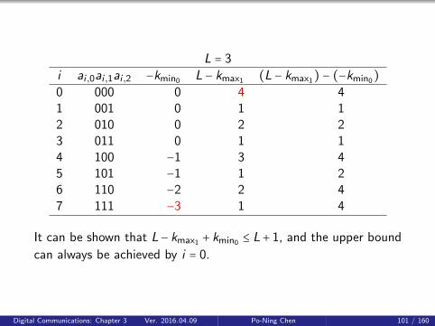
L = 3
i ai ,0ai ,1ai ,2 −kmin0 L − kmax1 (L − kmax1) − (−kmin0)
0 000 0 4 41 001 0 1 12 010 0 2 23 011 0 1 14 100 −1 3 45 101 −1 1 26 110 −2 2 47 111 −3 1 4
It can be shown that L− kmax1 + kmin0 ≤ L+ 1, and the upper bound
can always be achieved by i = 0.
Digital Communications: Chapter 3 Ver. 2016.04.09 Po-Ning Chen 101 / 160

Example. h = 1/2 and q(t) =
⎧⎪⎪⎪⎪⎨⎪⎪⎪⎪⎩
0 t < 0
t/(6T ) 0 ≤ t < 3T
1/2 otherwise
. Then
s0(t) =
⎧⎪⎪⎨⎪⎪⎩
sin ( π6T t) 0 ≤ t < 6T
0 otherwise
Ai ,n =n
∑k=−∞
Ik−2
∑k ′=0
ai ,k ′ In−k ′ and ci(t) =2
∏k ′=0
s0(t+k′T+ai ,k ′LT ).
Digital Communications: Chapter 3 Ver. 2016.04.09 Po-Ning Chen 102 / 160

ai,0ai,1ai,2 duration ci(t) e ı πhAi,n
0≡000 [0,4T) s0(t)s0(t +T )s0(t + 2T ) e ı θn+1
1≡001 [0,T) s0(t)s0(t +T )s0(t + 5T ) e ı (θn−2+πhIn+πhIn−1)
2≡010 [0,2T) s0(t)s0(t + 4T )s0(t + 2T ) e ı (θn−1+πhIn)
3≡011 [0,T) s0(t)s0(t + 4T )s0(t + 5T ) e ı (θn−2+πhIn)
4≡100 [-T,3T) s0(t + 3T )s0(t +T )s0(t + 2T ) e ı θn
5≡101 [-T,T) s0(t + 3T )s0(t +T )s0(t + 5T ) e ı (θn−2+πhIn−1)
6≡110 [-2T,2T) s0(t + 3T )s0(t + 4T )s0(t + 2T ) e ı θn−1
7≡111 [-3T,T) s0(t + 3T )s0(t + 4T )s0(t + 5T ) e ı θn−2
Note that⎧⎪⎪⎨⎪⎪⎩
c4(t) = c0(t +T )
e ı πhA4,n = e ı πhA0,n−1
⎧⎪⎪⎨⎪⎪⎩
c6(t) = c0(t + 2T )
e ı πhA6,n = e ı πhA0,n−2
⎧⎪⎪⎨⎪⎪⎩
c7(t) = c0(t + 3T )
e ı πhA7,n = e ı πhA0,n−3
and⎧⎪⎪⎨⎪⎪⎩
c5(t) = c2(t +T )
e ı πhA5,n = e ı πhA2,n−1
Digital Communications: Chapter 3 Ver. 2016.04.09 Po-Ning Chen 103 / 160

For nT ≤ t < (n + 1)T ,
sb-CPM,`(t) = e ı φ(t;I)=
7
∑i=0
e ı πhAi,nci(t − nT )
= e ı πhA0,nc0(t − nT ) + e ı πhA1,nc1(t − nT ) + e ı πhA2,nc2(t − nT )
+ e ı πhA3,nc3(t − nT ) + e ı πhA4,nc4(t − nT ) + e ı πhA5,nc5(t − nT )
+ e ı πhA6,nc6(t − nT ) + e ı πhA7,nc7(t − nT )
= e ı πhA0,nc0(t − nT ) + e ı πhA1,nc1(t − nT ) + e ı πhA2,nc2(t − nT )
+ e ı πhA3,nc3(t − nT ) + e ı πhA0,n−1c0(t − (n − 1)T )
+ e ı πhA2,n−1c2(t − (n − 1)T ) + e ı πhA0,n−2c0(t − (n − 2)T )
+ e ı πhA0,n−3c0(t − (n − 3)T )
=∞∑
m=−∞[e ı πhA0,mc0(t −mT ) + e ı πhA1,mc1(t −mT )
+e ı πhA2,mc2(t −mT ) + e ı πhA3,mc3(t −mT )]
=∞∑
m=−∞
⎡⎢⎢⎢⎢⎣
23−1−1
∑i=0
e ı πhAi,mci(t −mT )
⎤⎥⎥⎥⎥⎦
(for m = n − 3, n − 2, n − 1, n)
Digital Communications: Chapter 3 Ver. 2016.04.09 Po-Ning Chen 104 / 160

So, we notice that when ai ,0 = 1, ci(t) is always a shift-versionof some cj(t) with 0 ≤ j ≤ 2L−1 − 1.
This concludes to that:
Theorem 1 (Laurent ’86)
For nT ≤ t < (n + 1)T ,
sb-CPM,`(t) =∞∑
m=−∞
⎡⎢⎢⎢⎢⎣
2L−1−1
∑i=0
e ı πhAi,mci(t −mT )
⎤⎥⎥⎥⎥⎦
where
Ai ,n =n
∑k=−∞
Ik −L−1
∑k ′=1
ai ,k ′ In−k ′
and
ci(t) = s0(t)L−1
∏k ′=1
s0(t + k ′T + ai ,k ′LT )
with duration 0 ≤ t < (L − kmax1)T .
Digital Communications: Chapter 3 Ver. 2016.04.09 Po-Ning Chen 105 / 160

3.4 Power spectrum of digitalmodulated signals
Digital Communications: Chapter 3 Ver. 2016.04.09 Po-Ning Chen 106 / 160

Why studying spectral characteristics?
Bandwidth limitation in a real channel.
Random process Ô⇒ Power spectral density
PAMCPM
Digital Communications: Chapter 3 Ver. 2016.04.09 Po-Ning Chen 107 / 160

Power spectra of modulated signals
The modulated waveform s(t) is deterministic given theinformation sequence I , so only the information sequenceI = (. . . , I−2, I−1, I0, I1, I2, . . .) is random!For convenience, we denote the waveform atnT ≤ t < (n + 1)T as s(t − nT ; In) if the modulation ismemoryless, and as s(t − nT ; I n) if the modulation iswith memory, where I n = (. . . , In−2, In−1, In).
Digital Communications: Chapter 3 Ver. 2016.04.09 Po-Ning Chen 108 / 160

Hence, the modulated lowpass equivalent signal can beexpressed as
v `(t) =∞∑
n=−∞s(t − nT ; I n).
Note that v `(t) is usually not a (wide-sense) stationaryprocess but a cyclostationary process.
Its spectral characteristics is then determined by thetime-averaged autocorrelation function rather than the usualauthocorrelation function for a WSS proess.
Digital Communications: Chapter 3 Ver. 2016.04.09 Po-Ning Chen 109 / 160

2.7.2 Cyclostationary processes
Digital Communications: Chapter 3 Ver. 2016.04.09 Po-Ning Chen 110 / 160

How to model a waveform source that carries digitalinformation?
For example,
X (t) =∞∑
n=−∞an ⋅ g(t − nT )
where {an}∞n=−∞ is a discrete-time random sequence, and
g(t) is a deterministic pulse shaping function.
Digital Communications: Chapter 3 Ver. 2016.04.09 Po-Ning Chen 111 / 160

Cyclostationary processes
Given that {an}∞n=−∞ is WSS, what is the statistical property
of X (t)?
X (t) is not necessarily (strictly) stationary. Its meanbecomes periodic with period T :
E[X (t)] = E [∞∑
n=−∞ang(t − nT )] = µa
∞∑
n=−∞g(t−nT ) = E [X (t+KT )]
Autocorrelation function becomes periodic with period T
RX(t1, t2) = E [X (t1)X ∗(t2)]
=∞∑
n=−∞
∞∑
m=−∞E[ana∗m]g(t1 − nT )g(t2 −mT )
=∞∑
n=−∞
∞∑
m=−∞Ra(n −m)g(t1 − nT )g(t2 −mT )
= RX(t1 +KT , t2 +KT )
Digital Communications: Chapter 3 Ver. 2016.04.09 Po-Ning Chen 112 / 160
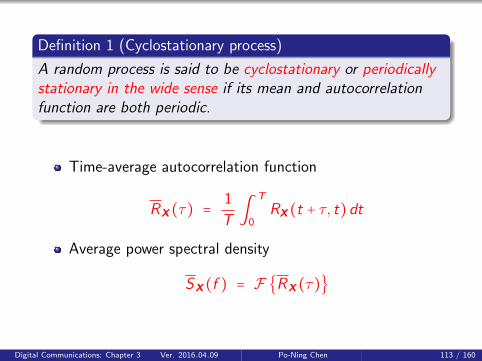
Definition 1 (Cyclostationary process)
A random process is said to be cyclostationary or periodicallystationary in the wide sense if its mean and autocorrelationfunction are both periodic.
Time-average autocorrelation function
RX(τ) =1
T ∫T
0RX(t + τ, t)dt
Average power spectral density
SX(f ) = F {RX(τ)}
Digital Communications: Chapter 3 Ver. 2016.04.09 Po-Ning Chen 113 / 160

3.4-1 Power spectral density of adigitally modulated signal with
memory
Digital Communications: Chapter 3 Ver. 2016.04.09 Po-Ning Chen 114 / 160

E [v `(t)] =∞∑
n=−∞E [In]g(t − nT ) = µI
∞∑
n=−∞g(t − nT ) = E [v `(t +T )]
and
Rv`(t1, t2) = E [v `(t1)v∗` (t2)]
=∞∑
n=−∞
∞∑
m=−∞E [InI
∗m]g(t1 − nT )g∗(t2 −mT ) = Rv`(t1 +T , t2 +T )
implies that v `(t) is cyclostationary.
Rv`(τ)
=1
T ∫T
0
∞∑
n=−∞
∞∑
m=−∞RI (n −m)g(t + τ − nT )g∗(t −mT )dt
=1
T ∫T
0
∞∑
k=−∞
∞∑
m=−∞RI (k)g(t + τ − kT −mT )g∗(t −mT )dt
(k = n −m)
Digital Communications: Chapter 3 Ver. 2016.04.09 Po-Ning Chen 115 / 160
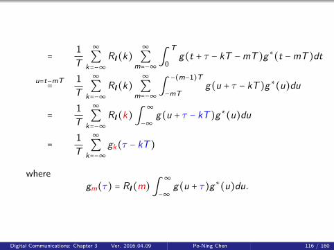
=1
T
∞∑
k=−∞RI (k)
∞∑
m=−∞∫
T
0g(t + τ − kT −mT )g∗(t −mT )dt
u=t−mT=
1
T
∞∑
k=−∞RI (k)
∞∑
m=−∞∫
−(m−1)T
−mTg(u + τ − kT )g∗(u)du
=1
T
∞∑
k=−∞RI (k)∫
∞
−∞g(u + τ − kT )g∗(u)du
=1
T
∞∑
k=−∞gk(τ − kT )
wheregm(τ) = RI (m)∫
∞
−∞g(u + τ)g∗(u)du.
Digital Communications: Chapter 3 Ver. 2016.04.09 Po-Ning Chen 116 / 160

Gm(f ) = ∫
∞
−∞gm(τ)e− ı2πf τdτ
= ∫
∞
−∞(RI (m)∫
∞
−∞g(u + τ)g∗(u)du) e− ı2πf τdτ
= RI (m)∫
∞
−∞(∫
∞
−∞g(u + τ)e− ı2πf τdτ)g∗(u)du
v=u+τ= RI (m)∫
∞
−∞(∫
∞
−∞g(v)e− ı2πf (v−u)dv)g∗(u)du
= RI (m) (∫
∞
−∞g(v)e− ı2πfvdv)(∫
∞
−∞g∗(u)e ı2πfudu)
= RI (m)∣G(f )∣2
⇒ Sv`(f ) = F {Rv`(τ)} =1
T
∞∑
k=−∞F {gk(τ − kT )}
=1
T
∞∑
k=−∞RI (k)∣G(f )∣2e− ı2πkfT
=1
TSI (f )∣G(f )∣2 where SI (f ) =
∞∑
k=−∞RI (k)e
− ı2πkfT .
Digital Communications: Chapter 3 Ver. 2016.04.09 Po-Ning Chen 117 / 160
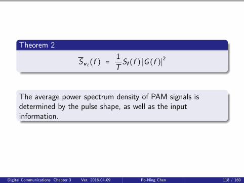
Theorem 2
Sv`(f ) =1
TSI(f ) ∣G(f )∣
2
The average power spectrum density of PAM signals isdetermined by the pulse shape, as well as the inputinformation.
Digital Communications: Chapter 3 Ver. 2016.04.09 Po-Ning Chen 118 / 160

Example
Input information is real and mutually uncorrelated
RI(k) = {σ2
I + µ2I , k = 0
µ2I , k ≠ 0
Hence
SI(f ) = σ2I + µ
2I
∞∑
k=−∞e− ı2πfkT = σ2
I +µ2
I
T
∞∑
k=−∞δ (f −
k
T)
and
Sv`(f ) =σ2
I
T∣G(f )∣
2+µ2
I
T 2
∞∑
k=−∞δ (f −
k
T) ∣G(f )∣
2
Digital Communications: Chapter 3 Ver. 2016.04.09 Po-Ning Chen 119 / 160

Sv`(f ) =σ2
I
T∣G(f )∣2
´¹¹¹¹¹¹¹¹¹¹¹¹¹¹¹¹¹¹¹¹¸¹¹¹¹¹¹¹¹¹¹¹¹¹¹¹¹¹¹¹¹¹¶continuous
+µ2
I
T 2
∞∑
k=−∞δ (f −
k
T) ∣G(f )∣2
´¹¹¹¹¹¹¹¹¹¹¹¹¹¹¹¹¹¹¹¹¹¹¹¹¹¹¹¹¹¹¹¹¹¹¹¹¹¹¹¹¹¹¹¹¹¹¹¹¹¹¹¹¹¹¹¹¹¹¹¹¹¹¹¹¹¹¹¹¹¹¹¹¹¹¹¹¹¹¹¹¸¹¹¹¹¹¹¹¹¹¹¹¹¹¹¹¹¹¹¹¹¹¹¹¹¹¹¹¹¹¹¹¹¹¹¹¹¹¹¹¹¹¹¹¹¹¹¹¹¹¹¹¹¹¹¹¹¹¹¹¹¹¹¹¹¹¹¹¹¹¹¹¹¹¹¹¹¹¹¹¹¹¶discrete
Observation 1: Discrete spectrum vanishes when theinput information has zero mean, which is often desirablefor digital modulation techniques under consideration.
Observation 2: With a zero-mean input information, theaverage power spectrum density is determined by G(f ).
Digital Communications: Chapter 3 Ver. 2016.04.09 Po-Ning Chen 120 / 160
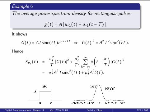
Example 6
The average power spectrum density for rectangular pulses
g(t) = A [u−1(t) − u−1(t −T )]
It shows
G(f ) = AT sinc(fT )e− ı πfT ⇒ ∣G(f )∣2 = A2T 2sinc2(fT ).
Hence
Sv`(f ) =σ2
IT
∣G(f )∣2 +µ2
IT 2
∞∑
k=−∞δ (f −
k
T) ∣G(f )∣2
= σ2I A
2T sinc2(fT ) + µ2
IA2δ(f ).
Digital Communications: Chapter 3 Ver. 2016.04.09 Po-Ning Chen 121 / 160

Example 7
The average power spectrum density for raised cosine pulse
g(t) =A
2[1 + cos(
2π
T(t −
T
2))] (u−1(t) − u−1(t −T )) .
It gives
G(f ) =AT
2sinc(fT )
1
1 − f 2T 2e− ı πfT .
Hence
Sv`(f ) =σ2
IT
∣G(f )∣2 +µ2
IT 2
∞∑
k=−∞δ (f −
k
T) ∣G(f )∣2
=σ2
I A2T sinc2(fT )
4(1 − f 2T 2)2+µ2
IA2
4δ(f ) +
µ2IA
2
16δ (f −
1
T) +
µ2IA
2
16δ (f +
1
T) .
Note: limx→±1sinc2(x)(1−x2)2 =
14
Digital Communications: Chapter 3 Ver. 2016.04.09 Po-Ning Chen 122 / 160

Digital Communications: Chapter 3 Ver. 2016.04.09 Po-Ning Chen 123 / 160

Comparison of the previous two examples
Broader side lobe
Faster decay in tail (f −6 < f −2)
Digital Communications: Chapter 3 Ver. 2016.04.09 Po-Ning Chen 124 / 160

Assume A = T = σ2I = 1 and µI = 0
Sv`(f )Sv`(0)
Digital Communications: Chapter 3 Ver. 2016.04.09 Po-Ning Chen 125 / 160

Assume A = T = σ2I = 1 and µI = 0
Sv`(f )Sv`(0)
Digital Communications: Chapter 3 Ver. 2016.04.09 Po-Ning Chen 126 / 160

Assume A = T = σ2I = 1 and µI = 0
The smoother (meaning, continuity of derivatives) thepulse shape, the greater the bandwidth efficiency (lowerbandwidth occupancy).
The raised cosine pulse shape will result in higherbandwidth efficiency than the rectangular pulse shape.
Digital Communications: Chapter 3 Ver. 2016.04.09 Po-Ning Chen 127 / 160

What if I correlated?
Example 8
In = bn + bn−1
where {bn} mutually uncorrelated with zero mean and unitvariance.
Then,
RI(k) =
⎧⎪⎪⎪⎪⎨⎪⎪⎪⎪⎩
2 k = 0
1 k = ±1
0 otherwise
SI(f ) = 2 + e ı2πfT + e− ı2πfT = 2 (1 + cos(2πfT )) = 4 cos2(πfT )
Sv`(f ) =1
T∣G(f )∣
2SI(f ) =
4
T∣G(f )∣
2cos2 (πfT )
Digital Communications: Chapter 3 Ver. 2016.04.09 Po-Ning Chen 128 / 160

Rectangular pulse shape with A = T = 1
Sv`(f )Sv`(0)
Digital Communications: Chapter 3 Ver. 2016.04.09 Po-Ning Chen 129 / 160

Rectangular pulse shape with A = T = 1
Dependence in transmitted information (not the originalinformation) can improve the bandwidth efficiency.
Sv`(f )Sv`(0)
Digital Communications: Chapter 3 Ver. 2016.04.09 Po-Ning Chen 130 / 160

Power spectra of CPFSK and CPM
CPM: Assume I i.i.d.
v `(t) = e ı φ(t;I)
where
φ(t; I ) = 2πh∞∑
k=−∞Ikq(t − kT )
Rv`(t1, t2)
= E [v `(t1)v∗` (t2)]
= E [e ı φ(t1,I)e− ı φ(t2,I)]
= E [exp( ı2πh∞∑
k=−∞Ik [q(t1 − kT ) − q(t2 − kT )])]
Digital Communications: Chapter 3 Ver. 2016.04.09 Po-Ning Chen 131 / 160

Rv`(t1, t2)
= E [∞∏
k=−∞exp ( ı2πhIk [q(t1 − kT ) − q(t2 − kT )])]
=∞∏
k=−∞E [exp ( ı2πhIk [q(t1 − kT ) − q(t2 − kT )])]
=∞∏
k=−∞[∑n∈S
Pn exp ( ı2πhn [q(t1 − kT ) − q(t2 − kT )])] ,
where Ik = n ∈ S and Pn ≜ Pr[Ik = n].
Rv`(τ) =1
T ∫T
0Rv`(t + τ, t)dt
=1
T ∫T
0
∞∏
k=−∞[∑n∈S
Pneı2πhn[q(t+τ−kT)−q(t−kT)]] dt.
Digital Communications: Chapter 3 Ver. 2016.04.09 Po-Ning Chen 132 / 160

Assume τ ≥ 0. For mT ≤ τ = ξ +mT < (m + 1)T and0 ≤ t < T (i.e., the range of integration)
t+τ −(m+1)T = t+ξ−T and t+τ −(m+1−L)T = t+ξ−(1−L)T .
Rv`(τ)
=1
T ∫T
0
max{m+1,0}∏
k=min{m+1−L,1−L}[∑n∈S
Pneı2πhn[q(t+τ−kT)−q(t−kT)]] dt
m≥0=
1
T ∫T
0
m+1
∏k=1−L
[∑n∈S
Pneı2πhn[q(t+τ−kT)−q(t−kT)]] dt.
Digital Communications: Chapter 3 Ver. 2016.04.09 Po-Ning Chen 133 / 160

Hermitian symmetry of Rv `(τ)
It suffices to derive Rv`(τ) for τ ≥ 0 because Rv`(−τ) = R∗v`(τ).
Proof:
R∗v`(τ) =
1
T ∫T
0E [e− ı2πh∑∞k=−∞ Ik [q(t+τ−kT)−q(t−kT)]
] dt
=1
T ∫T
0E [e ı2πh∑∞k=−∞ Ik [q(t−kT)−q(t+τ−kT)]
] dt
=1
T ∫T+τ
τE [e ı2πh∑∞k=−∞ Ik [q(v−τ−kT)−q(v−kT)]
] dv
(v = t + τ)
=1
T ∫T
0E [e ı2πh∑∞k=−∞ Ik [q(v−τ−kT)−q(v−kT)]
] dv
= Rv`(−τ).
Digital Communications: Chapter 3 Ver. 2016.04.09 Po-Ning Chen 134 / 160
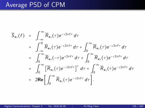
Average PSD of CPM
Sv`(f ) = ∫
∞
−∞Rv`(τ)e
− ı2πf τ dτ
= ∫
0
−∞Rv`(τ)e
− ı2πf τ dτ + ∫∞
0Rv`(τ)e
− ı2πf τ dτ
= ∫
∞
0Rv`(−τ)e
ı2πf τ dτ + ∫∞
0Rv`(τ)e
− ı2πf τ dτ
= ∫
∞
0[Rv`(τ)e
− ı2πf τ ]∗dτ + ∫
∞
0Rv`(τ)e
− ı2πf τ dτ
= 2Re [∫
∞
0Rv`(τ)e
− ı2πf τ dτ] .
Digital Communications: Chapter 3 Ver. 2016.04.09 Po-Ning Chen 135 / 160

∫
∞
0Rv`(τ)e
− ı2πf τ dτ
= ∫
LT
0Rv`(τ)e
− ı2πf τ dτ + ∫∞
LTRv`(τ)e
− ı2πf τ dτ
= ∫
LT
0Rv`(τ)e
− ı2πf τ dτ +∞∑m=L∫
(m+1)T
mTRv`(τ)e
− ı2πf τ dτ.
For m ≥ L, the two “regions” below are non-overlapping!
Digital Communications: Chapter 3 Ver. 2016.04.09 Po-Ning Chen 136 / 160

Rv`(τ)m≥L=
1
T ∫T
0
m+1
∏k=1−L
[∑n∈S
Pneı2πhn[q(t+τ−kT)−q(t−kT)]
] dt
=1
T ∫T
0(
0
∏k=1−L
[∑n∈S
Pneı2πhn[q(t+τ−kT)−q(t−kT)]
]
m−L∏k=1
[∑n∈S
Pneı2πhn[q(t+τ−kT)−q(t−kT)]
]
m+1
∏k=m+1−L
[∑n∈S
Pneı2πhn[q(t+τ−kT)−q(t−kT)]
])dt
=1
T ∫T
0(
0
∏k=1−L
[∑n∈S
Pneı2πhn[1/2−q(t−kT)]
]
m−L∏k=1
[∑n∈S
Pneı2πhn[1/2−0]
]
m+1
∏k=m+1−L
[∑n∈S
Pneı2πhn[q(t+τ−kT)−0]
])dt
Digital Communications: Chapter 3 Ver. 2016.04.09 Po-Ning Chen 137 / 160

Rv`(τ)m≥L=
1
T ∫T
0(
0
∏k=1−L
[∑n∈S
Pneı2πhn[1/2−q(t−kT)]
] [ΦI (h)]m−L
1
∏k ′=1−L
[∑n∈S
Pneı2πhn[q(t+τ−k ′T−mT)]
])dt (k ′ = k −m)
= [ΦI (h)]m−L λ(τ −mT ),
where ΦI (h) = ∑n∈S
Pneı πhn and
λ(ξ) =1
T ∫T
0(
0
∏k=1−L
[∑n∈S
Pneı2πhn[1/2−q(t−kT)]
]
1
∏k ′=1−L
[∑n∈S
Pneı2πhn[q(t+ξ−k ′T)]
])dt.
Digital Communications: Chapter 3 Ver. 2016.04.09 Po-Ning Chen 138 / 160

∞∑m=L∫
(m+1)T
mTRv`(τ)e
− ı2πf τ dτ
=∞∑m=L∫
(m+1)T
mT[ΦI (h)]
m−L λ(τ −mT )e− ı2πf τ dτ
=∞∑m=L∫
T
0[ΦI (h)]
m−L λ(ξ)e− ı2πf (ξ+mT) dξ (ξ = τ −mT )
= (∞∑m=L
[ΦI (h)]m−L e− ı2πfmT
)(∫
T
0λ(ξ)e− ı2πf ξdξ)
=
⎧⎪⎪⎪⎪⎪⎨⎪⎪⎪⎪⎪⎩
( e− ı 2πfLT
1−ΦI (h)e− ı 2πfT ) (∫T
0 λ(ξ)e− ı2πf ξdξ) if ∣ΦI (h)∣ < 1
(e− ı2πfLT∑∞m′=0 e
− ı2πT(f −ν/T)m′) (∫
T0 λ(ξ)e− ı2πf ξdξ)
if ∣ΦI (h)∣ = ∣e ı2πν ∣ = 1
=
⎧⎪⎪⎪⎪⎪⎨⎪⎪⎪⎪⎪⎩
( e− ı 2πfLT
1−ΦI (h)e− ı 2πfT ) (∫T
0 λ(ξ)e− ı2πf ξdξ) if ∣ΦI (h)∣ < 1
e− ı2πfLT (12 +
12T ∑
∞m′=−∞ δ (f −
ν+m′T ) − ı cot (πT (f − ν
T)))
(∫T
0 λ(ξ)e− ı2πf ξdξ) if ∣ΦI (h)∣ = ∣e ı2πν ∣ = 1
Digital Communications: Chapter 3 Ver. 2016.04.09 Po-Ning Chen 139 / 160

We finally obtain a numerically computable/plotable formula forthe average PSD of CPM. For example, if ∣ΦI (h)∣ < 1,
Sv`(f ) = 2 Re [∫
LT
0Rv`(τ)e
− ı2πf τ dτ
+(1
1 −ΦI (h)e− ı2πfT)(∫
T
0λ(ξ)e− ı2πf (ξ+LT)dξ)]
where for 0 ≤ τ = ξ +mT < LT ,
Rv`(τ)m≥0=
1
T ∫T
0
m+1
∏k=1−L
[∑n∈S
Pneı2πhn[q(t+τ−kT)−q(t−kT)]
] dt.
However, if ∣ΦI (h)∣ = ∣eı2πν ∣ = 1, where 0 ≤ ν < 1, the average PSDof CPM signals has impulses at fm′ = ν+m′
T for integer m′.
Digital Communications: Chapter 3 Ver. 2016.04.09 Po-Ning Chen 140 / 160
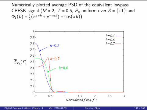
Numerically plotted average PSD of the equivalent lowpassCPFSK signal (M = 2, T = 0.5, Pn uniform over S = {±1} andΦI(h) =
12(e
ı πh + e− ı πh) = cos(πh))
Sv`(f )
Digital Communications: Chapter 3 Ver. 2016.04.09 Po-Ning Chen 141 / 160

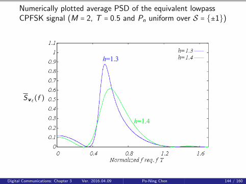
Numerically plotted average PSD of the equivalent lowpassCPFSK signal (M = 2, T = 0.5 and Pn uniform over S = {±1})
Sv`(f )
Digital Communications: Chapter 3 Ver. 2016.04.09 Po-Ning Chen 142 / 160

Numerically plotted average PSD of the equivalent lowpassCPFSK signal (M = 2, T = 0.5 and Pn uniform over S = {±1})
Sv`(f )
Digital Communications: Chapter 3 Ver. 2016.04.09 Po-Ning Chen 143 / 160
Numerically plotted average PSD of the equivalent lowpassCPFSK signal (M = 2, T = 0.5 and Pn uniform over S = {±1})
Sv`(f )
Digital Communications: Chapter 3 Ver. 2016.04.09 Po-Ning Chen 144 / 160

Observation 1
For h < 1
Its average PSD is relatively smooth and well confined.
Almost all power is confined within
fT < 0.6 or f <0.6
T
where T is the width of the channel symbols.
Digital Communications: Chapter 3 Ver. 2016.04.09 Po-Ning Chen 145 / 160
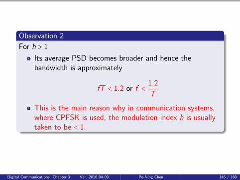
Observation 2
For h > 1
Its average PSD becomes broader and hence thebandwidth is approximately
fT < 1.2 or f <1.2
T
This is the main reason why in communication systems,where CPFSK is used, the modulation index h is usuallytaken to be < 1.
Digital Communications: Chapter 3 Ver. 2016.04.09 Po-Ning Chen 146 / 160

Example: Bluetooth RF specification (Version 1.0)
GFSK (Gaussian FSK) with BT = 0.5
B = Bandwidth (for baseband symbol) = 0.5 MHz,T = 1µ sec1 = positive frequency deviation0 = negative frequency deviation
Modulation index 0.28 ∼ 0.35
Modulation index = 2fdT , where fd is the peakfrequency deviation.0.28 < h = 2fdT < 0.35 Ô⇒ 140KHz < fd < 175KHzSymbol timing shall be better than ± 20 ppm.
Digital Communications: Chapter 3 Ver. 2016.04.09 Po-Ning Chen 147 / 160

Observation3
By letting h → 1
we can observe M impulses in the average PSD of theequivalent lowpass CPFSK signal.
Digital Communications: Chapter 3 Ver. 2016.04.09 Po-Ning Chen 148 / 160

Numerically plot-ted average PSD ofthe equivalent low-pass CPFSK signal(M = 4, Pn uniformover S = {±1,±3}and ΦI (h) =12(cos(πh)+cos(3πh)))
Approximately 4impulses appearwhen h ≈ 1.
The bandwidthbecomes broaderthan almost twiceof that of M = 2.
Digital Communications: Chapter 3 Ver. 2016.04.09 Po-Ning Chen 149 / 160

Approximately 8 impulses are observed when h ≈ 1.
Bandwidth becomes broader than almost four times ofthat of M = 2.
Digital Communications: Chapter 3 Ver. 2016.04.09 Po-Ning Chen 150 / 160

Re-visit MSK versus OQPSK
Sv`(f )Sv`(0) (dB)
Digital Communications: Chapter 3 Ver. 2016.04.09 Po-Ning Chen 151 / 160

Observations
Main Lobe: MSK is 50% wider than rectangular OQPSK,i.e., MSK = 1.5× rectangular OQPSK.
Side Lobe:
Compare the bandwidth that contains 99% of the totalpower: MSK = 1.2/T and rectangular OQPSK = 8.0/T .MSK decreases faster than OQPSK.MSK is significantly more bandwidth efficient thanrectangular OQPSK.By further decreasing the modulation index h (i.e.,making h < 1/2), the bandwidth efficiency of MSKs canbe increased. However, in such case MSK signals are nolonger orthogonal. Therefore, its error probability may
be increased. fd = 1/(4T )⇔ h = 2fdT = 1/2
Digital Communications: Chapter 3 Ver. 2016.04.09 Po-Ning Chen 152 / 160

Appendix: Fractional out-of-band power
Fractional in-band power
∆PIn-band(W ) =1
PTotal∫
W
−WSv`(f )df ,
where
PTotal = ∫
∞
−∞Sv`(f )df .
Fractional out-of-band power
∆POut-of-band(W ) = 1 −∆PIn-band(W )
This quantity is often used to measure the bandwidthefficiency of a modulation scheme. For example, findingthe bandwidth W under some acceptable condition, sayfractional-out-of-band power is no greater than 0.01.
Digital Communications: Chapter 3 Ver. 2016.04.09 Po-Ning Chen 153 / 160

Digital Communications: Chapter 3 Ver. 2016.04.09 Po-Ning Chen 154 / 160

Summary of spectral characteristics of CPFSK
signals
Modulation Index h
In general, the lower the modulation index h, the higherthe bandwidth efficiency.
Pulse shape g(t)
The smoother (meaning, e.g., continuity of thederivatives) the g(t), the greater the bandwidthefficiency.
For example, the raised cosine g(t) will result in higherbandwidth efficiency than the rectangular g(t).
For example, LRC (raised cosine g(t) with duration LT )with larger L (i.e., smoother) will result in greaterbandwidth efficiency.
Digital Communications: Chapter 3 Ver. 2016.04.09 Po-Ning Chen 155 / 160

Digital Communications: Chapter 3 Ver. 2016.04.09 Po-Ning Chen 156 / 160

Digital Communications: Chapter 3 Ver. 2016.04.09 Po-Ning Chen 157 / 160

What you learn from Chapter 3
(Pseudo-)Vectorization of standard ASK, PSK and QAMsignals
Computation of average energy based on signal spacevector pointsEuclidean distance based on signal space vector pointsGray code mapping from binary pattern to the signalspace vector points (in terms of their Euclideandistances)
(Good to know) QPSK versus π/4-QPSK
Digital Communications: Chapter 3 Ver. 2016.04.09 Po-Ning Chen 158 / 160
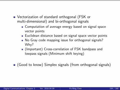
Vectorization of standard orthogonal (FSK ormulti-dimensional) and bi-orthogonal signals
Computation of average energy based on signal spacevector pointsEuclidean distance based on signal space vector pointsNo Gray code mapping issue for orthogonal signals?Why?(Important) Cross-correlation of FSK bandpass andlowpass signals (Minimum shift keying)
(Good to know) Simplex signals (from orthogonal signals)
Digital Communications: Chapter 3 Ver. 2016.04.09 Po-Ning Chen 159 / 160

(Important) Why cyclo-stationarity for digitallymodulated signals and its power spectrum
Modulation with memory – CPM signals
Its basic formation
φ(t; I) = 4πTfd ∫t
−∞d(τ)dτ
based on phase change d(t) = ∑∞n=−∞ Ing(t − nT )
(Good to know) Full response and partial responseMSK versus OQPSKLinear representation of CPM(Important) Time-average autocorrelation and powerspectrum (of cyclostationary PAM and MSK)
Digital Communications: Chapter 3 Ver. 2016.04.09 Po-Ning Chen 160 / 160


![II Baseband Modulation Schemes 020206[1]](https://img.pdfslide.us/doc/110x75/577d2a511a28ab4e1ea8f601/ii-baseband-modulation-schemes-0202061.jpg)