Embed Size (px)
Citation preview
I- NASA CR 3165 C.1
NASA Contractor Report 3165
Diffusion and Phase Change Characterization by Mass Spectrometry
Mark E. Koslin and Frederick A. White
GRANT NSG- 13 60 AUGUST 1979
https://ntrs.nasa.gov/search.jsp?R=19790020116 2018-08-04T02:49:56+00:00Z
TECH LIBRARY KAFB, NM
NASA Contractor Report 3165
Diffusion and Phase Change Characterization by Mass Spectrometry
Mark E. Koslin and Frederick A. White Rensselaer Polytechnic Institute Troy, New York
Prepared for Langley Research Center under Grant NSG- 1360
National Aeronautics and Space Administration
Scientific and Technical Information Branch
1979


TABLE OF CONTENTS
Page
PART I
PART II
PART III
PART IV
PART V
PART VI CONCLUSIONS .................................. 96
LIST OF TABLES ...............................
LIST OF FIGURES ..............................
INTRODUCTION .................................
ATOMIC DIFFUSION THEORY ......................
MATERIALS AND APPARATUS ......................
EXPERIMENTAL METHOD ..........................
RESULTS AND DISCUSSION .......................
iv
V
1
10
37
47
55
APPENDIXES ................................... 99
REFERENCES ................................... 102
iii

LIST OF TABLES
Table
Table
Table
Table
Table
Table
Table
Table
Table
Table
I
II
III
IV
V
VI
VII
VIII
IX
X
Page
Composition of 304 Stainless Steel......... 38
Composition of Tantalum.................... 39
Composition of Zircaloy-2.................. 40
Diffusion Coefficients of the Alkali Metals in Tantalum......................... 57
Diffusion Coefficients of the Alkali Metals in Zircaloy-2....................... 59
Diffusion Coefficients of the Alkali Metals in 304 Stainless Steel.............. 61
Do and Q for Impurity Diffusion in 304 Stainless Steel........................ 63
Do and Q for Impurity Diffusion in Tantalum................................... 64
Do and Q for Impurity Diffusion in Zircaloy-2...........................,..... 65
C-14 and Na-23 Diffusion in 304 Stain- less Steel................................. 91
Table XI Calculated Values of v and w............... 95
iv

I
Figure 1
Figure 2
Figure 3
Figure 4
Figure 5
Figure 6
Figure 7
Figure 8
Figure 9
Figure 10
Figure 11
Figure 12
Figure 13
Figure 14
Figure 15
Figure 16
Figure 17
LIST OF FIGURES
Page
DiffusiQn Mechanisms ......................
Mechanism for an Atomic Jump into a Vacancy ............................
Single Filament Thermal Ionization Source ....................................
Two-Stage Mass Spectrometer ...............
Schematic of Two-Stage Mass Spectrometer . .
Diffusion of Rb in Type 304 Stainless Steel .....................................
Activation Energy Diagram of Na-23 in Zircaloy-2 .............................
Activation Energy Diagram of K-39 in Zircaloy-2 .............................
Activation Energy Diagram of Rb-85 in Zircaloy-2 .............................
Activation Energy Diagram of Cs-133 in Zircaloy-2 .............................
Activation Energy Diagram of Li-7 in 304 Stainless Steel ....................
Activation Energy Diagram of Na-23 in 304 Stainless Steel ....................
Activation Energy Diagram of K-39 in 304 Stainless Steel ....................
Activation Energy Diagram of Rb-85 in 304 Stainless Steel ....................
Activation Energy Diagram of Cs-133 in 304 Stainless'Stee ....................
Activation Energy Diagram of Li-7 in Tantalum ...............................
Activation Energy Diagram of Na-23 in Tantalum ...............................
12
22
41
43
44
56
66
67
68
69
70
71
72
73
74
75
76
V
- --- .--.--.--.._. .

Page
Figure 18 Activation Energy Diagram of K-39 in Tantalum................................ 77
Figure 19 Activation Energy Diagram of Rb-85 in Tantalum................................ 78
Figure 20 Activation Energy Diagram of Cs-133 in Tantalum................................ 79
Figure 21 D vs. rimp(x) at Constant T('K) in Tantalum................................ 83
Figure 22 D vs. rimp(g) at Constant T('K) in Zircaloy-Z.............................. 86
Figure 23 D vs. rimp(R) at Constant T('K) in 304 Stainless Steel..................... 89
vi

Part I
INTRODUCTION
The mass spectrometer has long been used as an analyt-
ical tool in many disciplines. Relative to the space program,
the mass spectrometer was one of the first major analytical
instruments to be utilized from the very inception of the
nation's program.
Virtually every major rocket was equipped with a mass
spectrometer to measure the atmosphere either on ascent or
descent and in all recent missions the mass spectrometer has
provided a wealth of information which cannot be obtained with
any other type of instrumentation. Many types of mass spec-
trometers have monitored the upper atmosphere of the earth
and are continuing to do so. Additionally, deep space probes
can be expected to continue to utilize mass spectrometry, and
the surfaces of planets are amenable to analysis by mass
spectrometry via telemetering of their chemical composition.
Another major area in which mass spectrometry has made a
contribution to NASA sponsored programs relates to the high
purity materials that have been developed for solid state
electronics. Without mass spectrometric analysis to develop
a solid state technology, the rapid advance of transistors
and other microcircuitry, computers, etc. would not have
been possible, inasmuch as the mass spectrometer has a sensi-
tivity for analyzing trace elements that generally exceeds all

other analytical methodologies.
The present work, however, relates to a more generic
type of materials research that has applicability to high
strength metals and alloys for advanced space vehicles, and
even to the ultimate performance of composites in supersonic
transports. Hence, this research represents an even further
extension of the manifold applications for mass spectrometry
that have occurred during the last two decades.
Specifically, this paper addresses the problem of the
high temperature diffusion in metals, and it does so in a
very unique manner. Until the last few years, there was
rather little interest in the trace elements of metals as
opposed to some of the major constituents that are generally
recognized as alloying elements. However, we are now approach-
ing an era in which the efficiency and reliability of many
systems, e.g., freedom from corrosion, the attainment
of theoretical yield strengths, and the macroscopic properties
of materials generally are dependent upon trace metals and
their transport to grain boundaries. Hence, while this present
research effort is focused on a few specific materials, the
technology that it utilizes should have a very broad scale
application, and it is in this context that we are presenting
results of a preliminary nature which will hopefully lead to
an extended future study of diffusion in many engineering
materials.
We are pleased to acknowledge the technical input and
general Support from Dr. George M. Wood of the NASA-Langley
Research Center during the entire period of this investigation,

and for research funding from the National Aeronautics and
Space Administration under Research Grant NSG-1360.
The first basic theory for calculating diffusion coeffi-
cients was presented by Adolf Fick in 1855.l Fick who modified
Fourier's heat conduction equations, 2 hypothesized that in
an isotropic medium the quantity of diffusing substance Q,
which passes in a unit of time through a unit of transverse
cross sectional area, is proportional to the concentration
gradient measured along the normal to the section:
Q = -D(dC/dx) . (1)
The above equation is called Fick's first law for equilibrium
flow, C is the concentration of the diffusion substance in 3 units of mass/cm , x is the spatial coordinate in units of
cm., and D is the diffusion coefficient with units of cm2/sec.
In the case of non-equilibrium flow, Fick's second law can be
derived from the first law by considering the rate of accumula-
tion of the diffusing substance in a given element of volume
as the difference between the incoming and outgoing fluxes
per unit time. This yields
$$=D (2)
Fick's laws were shown to be approximations to more
general transport equations, and they may apply only to several
atomic distances from solute sources or sinks, when the solvent
is a homogeneous medium and when the solute concentrations are
small. 5 Boltzmann extended the application of Fick's equations
to large solute concentrations, 4 and these modified equations
were graphically solved by Matano 5 in 1936 for metallic
3

diffusion. To date, experimental determinations of the diffu-
sion coefficient have always followed a prescribed procedure.
The solute material was allowed to diffuse at a known temper-
ature and for a known time into a block of solvent material
of such a shape that Fick's laws yielded an exact mathematical
solution for the diffusion process in the system. Next, the
solute concentration was measured at known points throughout
the solvent. These values of solute concentration, and the
diffusion coefficient was found algebraically or graphically.
The problem of experimentally determining the diffusion co-
efficient thus became one of accurately determining the solute
concentrations throughout the solvent, and of fulfilling the
initial and boundary conditions applicable to a particular form
of Fick's laws.
The methods which various experimenters have used to
determine the solute concentrations and to satisfy the Fick's
law boundary conditions in their experiments are quite diverse.
An excellent summary of these different methods have been
compiled by Gertsriken and Dekhtyar. 6
The introduction of radioisotopes in the 1940's enabled
the concentration of a radioactive solute in a solvent
specimen to be determined quite readily by nuclear radiation
detectors. It is now advantageous to illustrate these
standard methods.
Serial Sectioning: This method involving radioactive tracers
is most frequently used in the study of diffusion. The sample
after being held at a given temperature for a known amount of
time (annealing time) to allow the radioactive tracer to
diffuse into the sample, is subjected to a series of sectioning
4

operations. The sample is weighed before and after each
cut to determine the thickness of the material removed.
The cuttings are collected and their activity measured with
a Geiger or scintillation counter. From the weights and
the density, the coordinates of the midpoints of each slice, .
(xl , are calculated. A plot of the natural logarithm of
the activity versus x2 has a slope of -1/4Dt for volume
diffusion. Hence, if the time of the anneal, t, is known,
the diffusion coefficient D may be calculated.
The main advantage of the serial sectioning method is
that it is simple, direct, and doesn't depend on the properties
of the radiation from the radioactive material used, assuming
no damage to substrate by ionizing radiation from the radio-
isotope.
Residual Activity Method: This method is similar to the .- -- serial sectioning analysis in that layers of thickness x
are removed, but the total remaining activity, I, of the
sample is measured in this case.
In the case of weakly absorbed radiation (strong gamma
rays) a plot of ln(-dI/dx) versus x should be a straight
line of slope -1/4Dt; and in the case of strongly absorbed
radiation (weak beta-rays) a plot of In(I) versus x L should
also be a straight line of slope -1/4Dt.
Surface Decrease Method: In this method, the total activity
of the specimen is measured as a function of time. No section-
ing of the sample is necessary.
5

Autoradiography: The principle of this method is to determine
the photographic density of the blackening of an exposed
emulsion as a function of the distance from the interface of
the specimen with the initial radioactive deposit. The speci-
men is usually cut at a measured angle a (usually 90') to the , initial face, and the cut face is placed in contact with a
piece of appropriate X-ray film. The blackening of the emulsion
(which is usually found to be directly proportional to the
cconcentration of activity) is measured with a micro-densitom-
eter. A plot of In (photographic density) versus x2 has a slope
of -1/4Dt from which D may be calculated if the anneal time,
t, is known. This method offered two distinct advantages; 1)
since the filament was small, the times involved in heating
and cooling it were small, and 2) because of the source mount-
ing and the high vacua of the mass spectrometer the diffusing
system was negligibly affected by any reaction between it and
the surrounding environment at the experimental operating
temperatures.
With the advent of sophisticated electronics, new devices
have been developed for studying solid state phenomena. The
electron-beam microprobe is one of the most important as far
as diffusion studies are concerned. The device collimates a
beam of electrons into a 1 l.~ diameter "pencil" which is
directed onto the specimen surface at the spot to be analyzed.
The electron bombardment causes characteristic X-rays to be
mitted from the sample. These X-rays are then detected and
analyzed to determine composition of the bombarded surface.
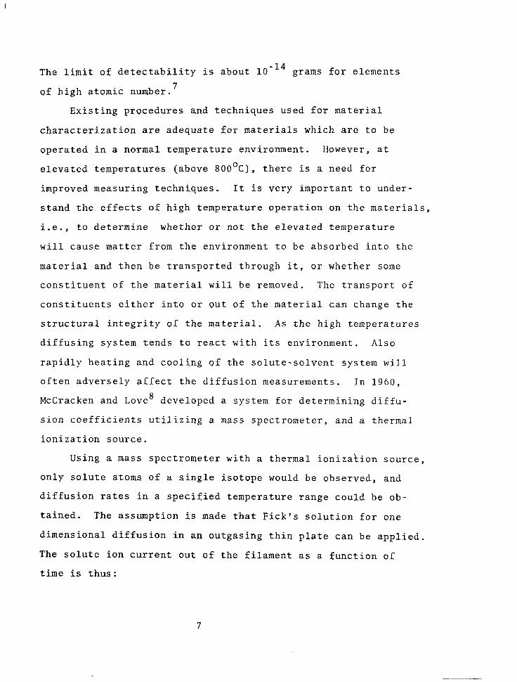
The limit of detectability is about lo-l4 grams for elements 7 of high atomic number.
Existing procedures and techniques used for material
characterization are adequate for materials which are to be
operated in a normal temperature environment. However, at
elevated temperatures (above 800°C), there is a need for
improved measuring techniques. It is very important to under-
stand the effects of high temperature operation on the materials,
i.e., to determine whether or not the elevated temperature
will cause matter from the environment to be absorbed into the
material and then be transported through it, or whether some
constituent of the material will be removed. The transport of
constituents either into or out of the material can change the
structural integrity of the material. As the high temperatures
diffusing system tends to react with its environment. Also
rapidly heating and cooling of the solute-solvent system will
often adversely affect the diffusion measurements. In 1960,
McCracken and Love8 developed a system for determining diffu-
sion coefficients utilizing a mass spectrometer, and a thermal
ionization source.
Using a mass spectrometer with a thermal ionization source,
Only solute atoms of a single isotope would be observed, and
diffusion rates in a specified temperature range could be ob-
tained. The assumption is made that Fick's solution for one
dimensional diffusion in an outgasing thin plate can be applied.
The solute ion current out of the filament as a function of
time is thus:

J- Ion = A exp (-r2Dt/x2) (3)
where A is a constant of proportionality, D is the diffusion
coefficient, x is the filament thickness, and t is the
measurement time. Hence, the slope of a plot of the natural
logarithm of the solute ion current versus time will yield
the desired diffusion coefficient, provided the thickness of
the filament is known. 9
General Advantages of the Mass Spectrometric Technique: There
were many reasons for choosing the mass spectrometric approach
for determining diffusion characteristics. As the mass
spectrometer analyzes one mass at a time, there is no ambiguity
caused by interfering masses. Since the filament is small,
the times involved in heating and cooling it are also small.
The probability of a reaction occuring between the high tem-
perature specimen and the surrounding environment is negligible
due to the mounting and the high vacua of the mass spectrometer.
Finally, the sensitivity of the instrument permits the impurity
level to be less than a part per billion, thus no doping of the
sample is necessary and commercial grade material can be
utilized.
Importance of Sample Materials: The materials studied in this
work were tantalum, zircalvy-2, and 304 stainless steel. These
materials were chosen for two basic reasons. First, they
represent a family of materials which go from being ultra pure
(99.996% Ta) to a 1.5% alloy with zirconium, to a 70% Fe,
8

18.5% Cr, 9% Ni, alloy (304 stainless steel). Hopefully,
this will enable one to draw conclusions about diffusion
rates in alloys rather than ultra-pure single crystals.
Secondly, these materials are of current interest to the
nuclear industry where higher operating temperatures mean
higher efficiencies.
The alkali metals were chosen as the elements of inter-
est primarily due to their relatively low ionization potential
(making them more suitable for thermal ionization) and due
to the fact that they probably appear in most materials as
naturally occurring impurities - thus eliminating doping of
the host matrix. It was decided that concentrating these
experiments on an entire chemical family might yield an over-
all diffusion mechanism which would allow diffusion rates of
other impurities and sample materials to be approximated.
Use of trade names or names of manufacturers in this
report does not constitute official endorsement of such
products or manufacturers, either expressed or implied,
by the National Aeronautics and Space Administration.

Part II
ATOMIC DIFFUSION THEORY
A. General Considerations
Diffusion is one of the mechanism by which matter
is transported through matter. From the theory of specific
heats, it is known that atoms in a crystal oscillate around
their equilibrium position. Occasionally these oscillations
become large enough to allow an atom to change sites. The
net result of many such random movements of a large number of
atoms is actual displacement of matter, the movement being
activated by the thermal energy of the crystal. 10 The path
of an individual particle is an unpredictable zigzag. The
length of an individual step in this zigzag is determined
in a solid by its jump length, b, i.e., the distance the
particle is able to move when it acquires enough energy to
make one jump.
The frequency of jumping, f, is the vibrational
frequency multiplied by the probability that the vibrating
atom has the activation energy to make the jump;
f = (1/3)w exp (GD/RT) (4)
where w is the vibrational frequency, l/3 allows roughly for
the fact that only about l/3 of the randomly directed vibra-
tions are in the required direction, and GD is the free
energy of activation, 11 From this we can obtain an equation
for the diffusion coefficient, D,
D = (l/2) b2f (5)
10

B. Diffusion Mechanisms
How the substance diffuses through the material is
just as important as the diffusion coefficient formula itself.
There are quite a variety of mechanisms by which an atom
can move from one position to another in a crystalline
structure.
Vacancy Mechanism: In all other than perfect crys-
tals, some of the lattice sites are unoccupied. These unoccu-
pied sites are called vacancies. If one of the atoms on an
adjacent site jumps into the vacancy, the atom is said to have
diffused by a vacancy mechanism, see Figure l(b).
Interstitial Mechanism: When small atoms dissolve
in metallic lattices as impurities so as to occupy inter-
stitial positions between solvent atoms and an atom passes
from one interstitial site to one of its nearest neighbor
interstitial sites without permanently displacing any of
the matrix atoms an interstitial mechanism is said to have
taken place. The interstitial mechanism is thought to
operate in alloys for those solute atoms which normally
occupy interstitial positions. It will be dominant in any
nonmetallic solid in which the diffusing interstitial
doesn't distort the lattice too much, 12 see Figure 1 (a).
Interchange or Exchange Mechanism: This is the
direct exchange of two nearest neighbor atoms.
Ring Mechanism: A more general form of the ex-
change mechanism consisting of a number (three or more) of
11

a b Interstitial Mechanism Vacancy Mechanism
0000 o- 0
0000
0 0 0000000 0 -0000000
0 8 0 0000000
oc..:;o C d
Interstitiality Mechanism Crowdion Mechanism
DIFFUSION MECHANISMS
Figure 1

atoms forming a closed ring. Atomic diffusion then takes
place by rotation of the ring.
Interstitialcy Mechanism: An interstitial atom
moves from an interstitial site to an adjacent normal
lattice site displacing the atom that had occupied that site
into a new interstitial site, see Figure 1 (c).
Crowdion Mechanism: A line imperfection consist-
ing of n nearest neighbor atoms compressed into a space
normally occupied by (n-l) atoms. Diffusion then takes
place by movement along the line of atoms, see Figure 1 (d).
Dislocation Mechanism: Dislocations can provide
easier paths for diffusion than a perfect lattice. The
diffusion of dislocated atoms can be produced in two ways:
1) the diffusion of the dislocated atoms over the inter-
stices and 2) displacement of the dislocated atom from the
interstice into a normal site of the lattice, and the atom
situated in the lattice goes over into the interstice.
C. Theoretical Methods of Diffusion Coefficient Calculations
While the mechanisms of diffusion may be summarized
from purely qualitative consideration, the problems involved
in quantitatively calculating a diffusion coefficient for a
specific solute-solvent system are quite complex. A con-
venient first step towards solving these problems is the
consideration of the rate at which the solvent atoms them-
selves move around in the solvent lattice, or the self-diffu-
sion coefficient of the solvent material. After a solution
13

has been found to the problem of self-diffusion, the effects
of a solute impurity are treated as a superposition problem.
The relationship between impurity diffusion coefficient and
the self-diffusion coefficient is discussed in section C-2.
C-l Self-Diffusion
Introduction: In a pure metal, diffusion operates
by the vacancy mechanism and the self-diffusion coefficient
is determined by the frequency with which an atom will jump
into a vacant neighboring site, w, and by the probability
that a given neighboring site is vacant, Pv. These experi-
ments are usually performed by plating a very thin film of
radioactive tracer on a pure metal, annealing, sectionino 09 and using the thin film solution to determine D,. 13 This
Ds is called the self-diffusion coefficient of the solute
in the given solvent, and the experiments are done ideally
at "infinite dilution." For the infinitely dilute alloy, the
problem is then to estimate whether and by how much w and
Pv for a solute atom differs from w and Pv for a solvent
atom.
c-1.1 Mathematical Model: A general approach to the
derivation of the diffusion coefficient is to consider the
problem as a whole sequence of jumps that result in paths of
atoms migrating through the lattice rather than merely
jumps between two planes. This concept is referred to as
the "random walk" approach.
14

Consider that successive atom jumps are vectors
? 1' f,, etc. If r is the total number of completed jumps
which an atom makes per unit time, then after a time t, a
total of n = tr completed jumps will have occurred, and the
atom will have moved an average distance, m
R(t) = Zri (6)
from its initial position. It may be shown that the diffusion
coefficient, D, is obtained by
D= R(t)2/6t (7)
where RTj2 = (ii(t) - ii(t) 1 .
Now m2 = z.v2
-2 = r. 1
+ 2LZri . r. i+j ' (8)
For the case of the fee, bee, and hcp crystal systems, all
the jump vectors will be of equal magnitude, r. Then
equation (8) may be written as
m2= nr2 + 2r2Z(n-j) cos 9 j (9)
where cos 8. is the average value of the cosine of the angle
between theJith and the ( i + j ) t11 atom jump.
If the direction of each jump is independent of
all earlier jumps, then cos e. 3
= 0 and substituting equation
(9) into equation (7) we obtain
D= ( l/6 ) r'r2 . (10)
The factor ( l/6 ) come from the fact that only l/3 of the
randomly directed vibrations are in the required direction,
and then substituted into equation (5).
15

As an example, consider an fee lattice. For this case r =
12wN, where 12 is the number of nearest neighbors, w is the
jump frequency, and Nv is the fraction of vacant sites.
With a lattice constant ao, for vacancy diffusion
D = ai N,w ,
while for interstitial diffusion
with d being a geometric constant. 14
The problem of determining D has now been reduced
to finding a way of calculating NV and w .
c-1.2 Correlation Effects: The assumption of uncorrela-
ted motion made in the derivation of equation (9) is valid
for interstitial diffusion in dilute alloys. However, it is
not valid in the case of vacancy or interstitialcy diffusion.
Consider vacancy diffusion, after an exchange between an
impurity atom and a vacancy all of its neighbors are not
identical; one of them consists of a vacancy, it is most
probable that the impurity atom will jump back to the position
occupied by the vacancy. In other words, the mean square dis-
placement for the impurity atom after n jumps, ai, will be
less than that for a vacancy which took the same number of
jumps, K: = nr2. The ratio of these two quantities defines
the correlation factor, f, as
(11)
16

The correlation factor has been calculated by
Compaan and Haven.l' They demonstrated that the correlation
factor could be written as
f = 1 + COS ei / l - coS ei (12)
where cos ei refers to the average of the cosine of the
angle between consecutive jumps. For vacancy diffusion in
a fee lattice, where the terms have been previously defined,
D= a:fwNv .
c-1.3 Calculation of NV: According to classical ther-
modynamics, a given system tends to assume a configuration
such that the free energy of the system is a minimum. This -
free energy G is related to the enthalpy, H, temperature in
degrees Kelvin, T, and entropy, S, of the system by
G =H-TS Cl31
The entropy of any system may be divided into two
parts, the thermal entropy St and the configurational
entropy SC. The thermal entropy St is determined by the
number of different ways Wt in which the thermal energy of
the crystal may be distributed over the possible vibrational
modes of the individual atoms. Wt is related to St by the
Boltzmann relation, where k is Boltzmann's constant,
St = k In Wt . (14)
The configurational entropy of a crystal SC is determined by
the number of different ways WC in which the atoms of the
17

crystal may be arranged over the available number of lattice
sites. For the case of vacancies in a crystal, let N, be
the number of atoms in the crystal and nv be the number of
vacancies, and let all of the lattice sites be equivalent.
It can be then shown that this case 16
WC = (Na + nv)!
(N,! nv!) s (15)
Again the relation between SC and Wc is given by the
Boltzmann relation
sC
INa = k ln WC = k In N , + nv)!
( a' "v' ,) . (161
Now assume the energy to create a vacancy in a crystal to be
h V’ The enthalpy of a single crystal containing nv vacancies
is increased by a factor nvhv over that of a perfect crystal.
For reasons given below, the thermal entropy will increase
by a factor nvAst when nv vacancies are added to the crystal.
Thus, from these considerations and from equations (13) and
(16), the free energy of an imperfect crystal as a function
of nv and T becomes,
(Na G(n,T) = GperfectU) + nvhv - nvTAst - k In ma!
+ nv)! n v!)
(17)
In order to find the equilibrium value of nv, we note that
at equilibrium aG/anv = 0. Using this fact, and the approx-
imation that In x! = x In x for x < 1, we have from (17)17
Note: Lower case letters indicate a property of a single crystal, while a capital letter indicates a property of an entire crystalline structure.
18

"V n
n +N V a eq = <eq
ASt -hv = exp 7 exp T . (181
Here, (nv/Na> eq is the equilibrium atomic fraction of
vacancies in the crystal. In terms of the equilibrium mole
fraction of vacancies NV, equation (18) may be written
NV
Ast = exp.T -HV expT - 119)
In equation (19), AS, and Hv refer to the thermal entropy and
enthalpy changes of the entire crystal due to the addition of
NV vacancies.
It should be noted that the foregoing derivation
assumed that st and h, are independent of nv/Na, which
would be true if nv/Na, or N,, were very small. Experiment-
ally, NV has been found to be about 10 -4 in pure metals, 18
so this assumption is a reasonable one.
The enthalpy of a crystal should change with the
addition of a vacancy, and this energy change equals approxi-
mately the energy necessary to remove an atom from the inter-
ior of the crystal and place it on the crystal surface. The
reason for the change in St, however, is more subtle, One
way to estimate this change is to assume an Einstein model
for the solid consisting of N atoms equally distributed over
3N harmonic oscillators. 19 When w is the Einstein frequency
of the atoms in a perfect crystal and hw << k, where h is
Plank'sconstant, and k is Boltzmann's constant, then S t, the
thermal entropy can be shown to be"
19

st = 3N,k 11 + In El p1
for that perfect crystal. In a crystal containing nv
the atoms around a vacancy will have a vibra-
tional frequency v’ less than v because the atomic restoring
forces are reduced. Again using the Einstein model, each
atom neighboring a vacancy is assumed equivalent to 3
harmonic oscillators of frequency u’ . For Na atoms and
n v vacancies in a crystal, we have
3n,x oscillators of frequency v
(3N, - 3nvx) oscillators of frequency u’
where x is the number of nearest neighbor atoms around eac.h
vacancy. Applying this to equation (20), we have that the
thermal entropy of an imperfect crystal is:
st = 3nvxk 11 + In El + (3N, - 3nvx)k 11 + In E,/
(211
The change in thermal entropy due to the addition of nv
vacancies to a perfect crystal can be estimated by subtract-
ing (20) from (21) and dividing by nv to obtain
st = 3xk In (w/w’) . (221
Thus the change in thermal entropy is due primarily to the
change in vibrational frequency of the atoms around the
vacancies.
20

Calculation of w: While the calculation of Nv is a
straightforward one, accurate determination of the atomic
jump frequency for a tracer atom is quite difficult. In
fact, the accuracy of the present calculations of w is so
poor that such calculations provide no real verification of
experimentally determined diffusion coefficients. However,
the following relatively simple theoretical treatment of
w yields a numerical value of this parameter within at
least an order of magnitude, and it further provides some
insight into the temperature dependence of this quantity.
First, assume a simplified sequence of atomic motions
required for a tracer atom to jump from one lattice site
to another, as shown in sequence Figures Za, Zb, and 2c.
Before such a sequence can occur, the tracer atom must
attempt a jump in the direction of the vacant site, with
the two restraining atoms simultaneously moving far enough
apart to let the tracer atom slide between them. The
atomic configuration shown in Figure 2b is called an
activated complex, --- and consists of a region containing a
diffusing atom between two equilibrium sites. The number
of atoms diffusing per second in one mole of solvent
material equals the mole fraction of activated complexes
N m, multiplied by the average velocity of the diffusion atoms
moving between the restraining atoms v, divided by the
width of the barrier created by these restraining atoms 6.
21

88 0 0
a b
0 0 8 0 0
0 0 88
C
1 I L 1 r a b C
Free Energy Variation of Lattice During Sequence of Atomic Motions Shown in a, b, and c
MI:~I~ANTSM FOR AN ATOMIC JlrMP INTO A VACANCY
Figure 2
22

The average jump frequency per atom, w, becomes
w = N,;/ 6 (23)
To find an approximate value of Nm, it is assumed
that diffusing atoms enter, remain at, and leave the acti-
vated complex slowly so that the remainder of the lattice
has time to continually relax to an equilibrium state. 21
Using this assumption, the work done during the resulting
reversible, isothermal process of moving an impurity atom
from one site to another is just equal to the change in the
Gibbs free energy for the region, Gm. From these assumptions,
at any temperature, there will always be an equilibrium
number of activated complexes. From the definition of Gm,
in equation (13)
Gm = Hm - TSm (24)
Since the lattice was assumed to be in thermal equilibrium,
G, will have all of the properties of Gv of equation (17).
By a process identical to the derivation of equation (19)
from equation (17), 22 we can obtain the equilibrium mole
fraction of activated complexes at any instant:
Nm = exp 1 -Hi + TASK
I -AG,
= exp 1 - I RT RT
(251
In equation (23), a dimensional analysis will reveal that
i/a is a frequency. This frequency is conveniently taken
to be the mean vibrational frequency of an atom about its
23

equilibrium site, w, and represents the frequency with which
an atom attempts to change sites. From this and from
equations (23) and (25) we find
W = v exp -Hm + TASK
(261 RT
It has been determined experimentally that the
activated complexes do not exist long enough for much of the
surrounding lattice to reach equilibrium. 23 Thus, it would
seem that the basis for the derivation of equation (26) is
open to serious question. However, it does yield an order
of magnitude agreement with experiment.
C-2 Relationship Between Self-Diffusion and Dilute
Impurity Diffusion
The problems involved with impurity diffusion are
more complex than those of self-diffusion, since the atoms
of both solvent and solute migrate simultaneously. The mi-
gration of solute atoms is influenced by that of solvent atoms,
and the presence of impurity atoms in the lattice, changes
the energy conditions, and thus influences the rate of self-
diffusion.
c-2.1 Correlation Effects: In dilute alloys, the
vacancies are partially bound to the solute atoms, so that
there is in addition to the correlation between the jumps of
the solute atoms a correlation between the successive jumps
of the vacancies. Thus, it is no longer possible for P, to
24

equal NV, although these two quantities are still closely
related. Also, the correlation coefficient becomes much
less than unity. In this discussion of impurity diffusion,
it is assumed that the solute concentration is so small
that the diffusion coefficient of the solute in the solvent
lattice, or the impurity diffusion coefficient, is inde-
pendent of the solute concentration. In analyzing the
behavior of a solute atom-vacancy pair in a solvent lattice
under these conditions, the frequency with which the solute
atom and vacancy exchange positions may be taken as wl, the
frequency with which the vacancy exchanges places with a
nearest neighbor atom to the solute atom as w2, and the
frequency with which the vacancy exchange places with a
solvent atom which is not a nearest neighbor to the solute
atom as w 3' Thus w3 is proportional to the frequency at
which the solute atom-vacancy pair dissociates. Now if the
vacancy is tightly bound to the solute atom, w3 will be
nearly zero, and w1 will be much greater than w2. In other
words, if a vacancy exchanges places with a solute atom
with a given jump, the probability that it will reverse
that exchange with its next jump is nearly unity. If this
is so, the vacancy movement is nearly completely correlated,
and the solute atom will move through the lattice only as
fast as the vacancy exchanges with the solvent atoms. Thus,
the impurity diffusion coefficient for small solute con-
centrations, D I (0), will not be given by
25
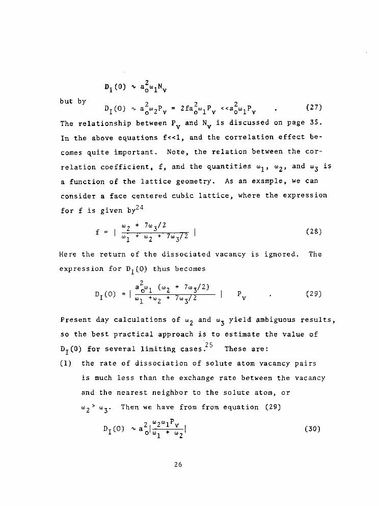
D I (0) s a'w N olv but by 2 DI(0) Q a w P 0 2 v = 2fa2w P olv <<a2w P olv * (27)
The relationship between P, and NV is discussed on page 35.
In the above equations f<<l, and the correlation effect be-
comes quite important. Note, the relation between the cor-
relation coefficient, f, and the quantities wl, w2, and w3 is
a function of the lattice geometry. As an example, we can
consider a face centered cubic lattice, where the expression
for f is given by24
f-1 w2 + 7w3/2 w1 + w2 + 7w3/2 I (28)
Here the return of the dissociated vacancy is ignored. The
expression for DI(0) thus becomes
2 D,(O) = 1 I;w;w
(w2 + 7w3/2) 2 + 7w 3/2 1 pv - (291
Present day calculations of w2 and o3 yield ambiguous results,
so the best practical approach is to estimate the value of -25 DI(0) for several limiting cases. These are:
(1) the rate of dissociation of solute atom vacancy pairs
is much less than the exchange rate between the vacancy
and the nearest neighbor to the solute atom, or
w2' w3. Then we have from from equation (29)
2 w2U1pv +(O) 'L aolw + w I 12
(39)
26

(2) the vacancy-solute atom exchange rate is much more
rapid than the two vacancy-solvent atom exchange rates,
or the vacancy-solute atom pair is tightly bound. Then
w1>>(w2 + 7w3/2) in (28), and we have
D I (0) Q az(w2 + 7w3/2)P V (31)
(w2 + 7w3/2) in (3) the solute atom jumps slowly, or wl<<
equation (29). Thus
2 D (0) 'L a w P I 01 v (32)
(4) the "solute" is a solvent tracer, so that wl = w2 = w3 =
W. Then, since here P, = NV, and D,(O) = DI(0)
D,(O) = 2faiNvw . (33)
It must be emphasized that the above results are
for a face centered cubic lattice. Other lattice geometries
will give results of essentially the same form, but with
different numerical constants.
c-2.2 Valence Effects: Due to the electronic effect of
an impurity atom with a valence different than that of the
surrounding host lattice a vacancy is often attracted to
the solute atom. Consider the case of a divalent impurity
in a monovalent lattice. According to the free electron
theory of metals the free electron density in the immediate
environment of the impurity will be greater than that
throughout the lattice as a whole, but it will not be great
27

enough to completely neutralize the excess positive charge
of the solute ion. This ion is said to be “screened,” and
it is surrounded by an electrostatic potential of the form
W-1 = (Ze/r 1 exp (-qV ) . (34)
Where r is the radial distance from the impurity ion, Z is
the number of excess electrons per impurity ion and q is
the screening parameter, which gives a measure of the
neutralization of the excess charge of the impurity ion.
Let a solvent atom be removed from a site adjacent to the
solute ion, and make the assumption that the electron dis-
tribution throughout the lattice will not be appreciably
distributed by this removal. If this is the case, the
vacancy resulting from this removal will have an effective
charge of -e. Its energy on the site next to the impurity
ion then will be reduced by
eV(rl = E(r) = ( Ze2/r 1 exp ( -qr I (35)
as compared to a site surrounded by normal solvent atoms.
Since the energy of the vacancy is lower next to the
impurity ion, the concentration of vacancies on any nearest
neighbor site will be increased to
pV = NV exp (E(r )/kT) . (36)
This effect will also decrease H, on a site next to a solute
atom by E(r ) as compared to H, on a site surrounded by
solvent atoms. This decrease in potential energy also makes
28

H, for the solute less than Hv for the solvent. Finally,
there is a force e(dV/dr) tending to draw the vacancy and
the impurity ion together. If the impurity ion and the
vacancy begin to move together, this force tends to pull
them together until Hv is decreased by roughly roe(dV/dr),,, .26 0
C-2.3 Size Effects: The effects on the impurity dif-
fusion coefficient of the size of the solute atom relative
to that of the solvent atom have been considered by Swalin 27
and Overhauser. 28
Swalin assumes that the solute atoms are com-
pressible spheres and the solvent lattice is an elastic con-
tinuum. For example, if the solute is larger than the
solvent atom, Hv will be increased by the additional strain
required at the saddle point. This change in Hv is a
balance between the strain on the diffusing solute atom and
the lattice continuum. Although it would seem that a large
solute atom would elastically strain the lattice and thereby
attract vacancies and lower H v, Stialin concluded that the
actual change in Hv is negligible to a first order approxi-
mation. 27
Overhauser 28 considered the effects on the
impurity diffusion coefficient of the presence of inter-
stitials in the solvent lattice. Since these interstitials
dilate the lattice locally, the average interatomic dis-
tance between the matrix atoms will be increased. This
lattice expansion will reduce the work required to squeeze
29

I-- II -m-m.--. mm. -.,mm.m.-- .-.-- ,_-._ , . . . . . . ._. . .._- . . . . ..---.-.--..-.-- --.-.
an atom through the saddle point, so Hv should be decreased
by the addition of an interstitial solute whose atoms are
larger than those of the solvent. Likewise, the addition
of an interstitial solute which contracts the solvent
lattice should increase H,.
Although the impurity diffusion concept has been
studied in detail for many elements, no single correlation
between diffusion parameters Do, the frequency factor, and Q,
the activation energy and the properties such as valence and
size has been found to fit more than one or two elements.
C-2.4 Solute Concentration Effects: When the solute
concentration becomes greater than some threshold value,
(which varies for different systems), the solute atoms begin
to interact and the diffusion coefficient for the solute as
well as the self-diffusion coefficient for the solvent
material becomes a function of the solute concentration.
In order to obtain a qualitative concept of the nature of
these functions, we consider the previously presented
equations for the self-diffusion of the pure solvent , (331,
and the dilute impurity diffusion coefficient for the solute,
in a face centered cubic solvent lattice, (28), i.e.,
2 Ds(0) = 2faowoNv (33)
and ao 1 2 (w
DIW = 21, + w 1
30

Now if Pv = NV and wl %LW~. - ~3, then no matter how large wl
is, D,(O) will about equal DI(0). However, if DI(0) is
greater that Ds(0) in very dilute alloys, it follows that
the impurity atoms attract vacancies so that Pv > Nv. Then
the solvent jump frequencies w2 and w1 are increased near
a solute atom. But if Pv > Nv, or w2 > w. near a solute
atom, then Ds is also greater near a solute atom. As the
solute concentration increases, so does the number of affected
solvent atoms. Thus, if DI (0) < D, (01, an addition of solute
will increase Ds. Similarly, if DI(0) > Ds(0), an addition
of solute will decrease D,.
To provide an estimate of the magnitude of the
change in the self-diffusion coefficient, Ds, with solute
concentration, the following empirical equations have been
derived for solute concentration 2 0.01:2g
DS =(l - ANI I( Ds (01) + ABNIDI (37)
DI = DIW (38)
Here, NI is the solute concentration, A is the number of
nearest neighbor sites around each atom, and B is an arbi-
trary constant < 1.0 which must be experimentally determined. - Thus, DI does not vary much with solute concentration for
solute concentrations less than 0.01. For solute concentra-
tions greater than 0.01, the relation between the impurity
diffusion coefficient and solute concentration is given by
DI = DI (0) ( 1 + I+ 1 (391
31

Here, p is a constant < 1.0. The values of the constants B -
and JJ vary from system to system. Specific theoretical
calculations of their values are quite difficult and are
not usually attempted.
D. Summary of Equations for Diffusion Coefficient
The following comprise a summary of the most use-
ful previously derived diffusion relationships which are
most useful in comparing experimentally observable parameters
with theoretical models for the diffusion process.
For vacancy self-diffusion in a pure solvent with
correlated tracer jumps, the self-diffusion coefficient, Ds,
is given by
Ds (01 = 2faiNvw (40)
-where f is the correlation coefficient, NV is the equili-
brium vacancy concentration, w is the tracer jump frequency,
and a0 is the lattice constant. For dilute impurity vacancy
diffusion, the diffusion coefficient of the solute in the
solvent lattice is
DI (01 = ZfazwlPv (41)
Here w1 is the frequency with which a solute atom changes
places with a nearest neighborvacancy, and Pv is the
probability that a nearest neighbor site to the impurity
atom is vacant. Because of attractive forces between the
vacancies and solute atoms have already been discussed, Pv
32

in equation (27) will not equal NV. An estimate 'of the
value of Pv in terms of NV for a given solvent-solute sys-
tem may be obtained from equations (33), (34), and (35).
The coefficient of correlation f is a function of lattice
geometry. For self-diffusion, f lies between 0.50 and 0.79;15
for a face-centered cubic solvent structure, f for impurity
vacancy diffusion is given by
f= w2 + 7w3/2 u1 + w2 + 7w3 (42)
Here w2 is the frequency with which a vacancy exchanges
position with a nearest neighbor atom to a solute atom, and
w3 is the frequency with which a vacancy exchanges position
with a solvent atom, which is not a nearest neighbor to a
solute atom.
From equilibrium thermodynamics, the equilibrium
vacancy concentration in a crystal was found to be
NV = Ast -HV
exp R ew RT - (43)
In a similar manner, an equilibrium approximation allowed
us to arrive at an expression for
a, = -H, + TASm
v exp -RT . (44)
Combining equations (19), (26), and (40) allows us to write
for the vacancy self-diffusion coefficient in a pure or
very dilutely contaminated solvent
33

Asf + As D, (0) =Zfatvexp 1 R m lexp 1 -Hf RTHml. (45)
Likewise, combining equations (19), (26) , (27) , and (35) , we
find for dilute impurity vacancy diffusion
DL(0) = 2faz v expl Asf + AS -H - -H, R ml exp I & j explql.
(46)
Here E(r ) may be estimated from equation (34), and f for a
fee lattice is given by equation (28). Generally, f will be
given in terms of the various jump frequencies described
above. Of these frequencies, only w1 can be calculated with
reasonable certainty; because of uncertainties in the values
of w2 and w 3, the usual practice is to consider the behavior
of DL(0) in the limiting cases given in equations (30), (31))
and (32).
Equations (37)) (38), and (39) give the variation
in the solvent self-diffusion coefficient Ds(0), and vacancy
impurity diffusion coefficient, D,(O), with solute concentra-
tion. Finally, for interstitial diffusion, the diffusion
coefficient, D, is given by
D= aivexp I- “21 exp I*] . (47)
Thus, interstitial diffusion can be considered a much simpler
process than vacancy diffusion. For the present investigation
it is probable that both vacancy and interstitial diffusion
mechanisms take place.
34

Equations (45), (46), and (47) are useful in cal-
culating values of D from theoretical models of the diffusion
process. To check the validity of a given model, a compari-
son is made of the calculated values of the factors compri-
sing D with corresponding experimentally determined values.
Several workers have devised experimental methods for deter-
mining the individual terms of equations (45), (46), and
(47), such as *Sf, AS,, Hm, etc.. However, the most common
procedure is first to express these equations in the form
D = Do exp ( -Q/RT ) . (48)
Then, after determining the diffusion coefficients of the
system under consideration at different temperatures, Q may
be found from the slope of the plot of the natural logarithm -1 of D versus ( temperature,'K ) , while the intercept of this
plot with the ordinate axis yields Do. The quantity Q is
called the activation energy, and is the sum of the enthalpy
terms in each of the equations for D, (45), (46), and (47).
This quantity is thus associated with the energy necessary
for the solute ion to make a single jump in the solvent lat-
tice. The symbol, Do, called the frequency factor, contains
the correlation coefficient, jump attempt frequency, lattice
parameter, and the entropy changes associated with an atomic
juv. Hence, Do gives a measure of the disorder induced in
the solvent lattice by an atomic jump.
35

The " random walk W is not the only approach for
the explanation of the phenomena of diffusion. Some of the
more interesting theories are presented by: Feit discusses a
dynamical theory,30931 Huntington and Seitz with a discussion
from the modern theory of metals, 32 Lazarus discusses the
effect of " screened 'I electrons on diffusion,55 Johnson
presents a " hole " theory for diffusion, 34
while Zener
presents a model for ring diffusion. 35
All of these studies
present arguments which are valid for some very limited
cases and were therefore not used in this work. For further
reading on diffusion, 36
the studies by LeClaire , Wert and 37
Zener, Turnbull and Hoffman, 38
and Zener 39
are suggested.
36
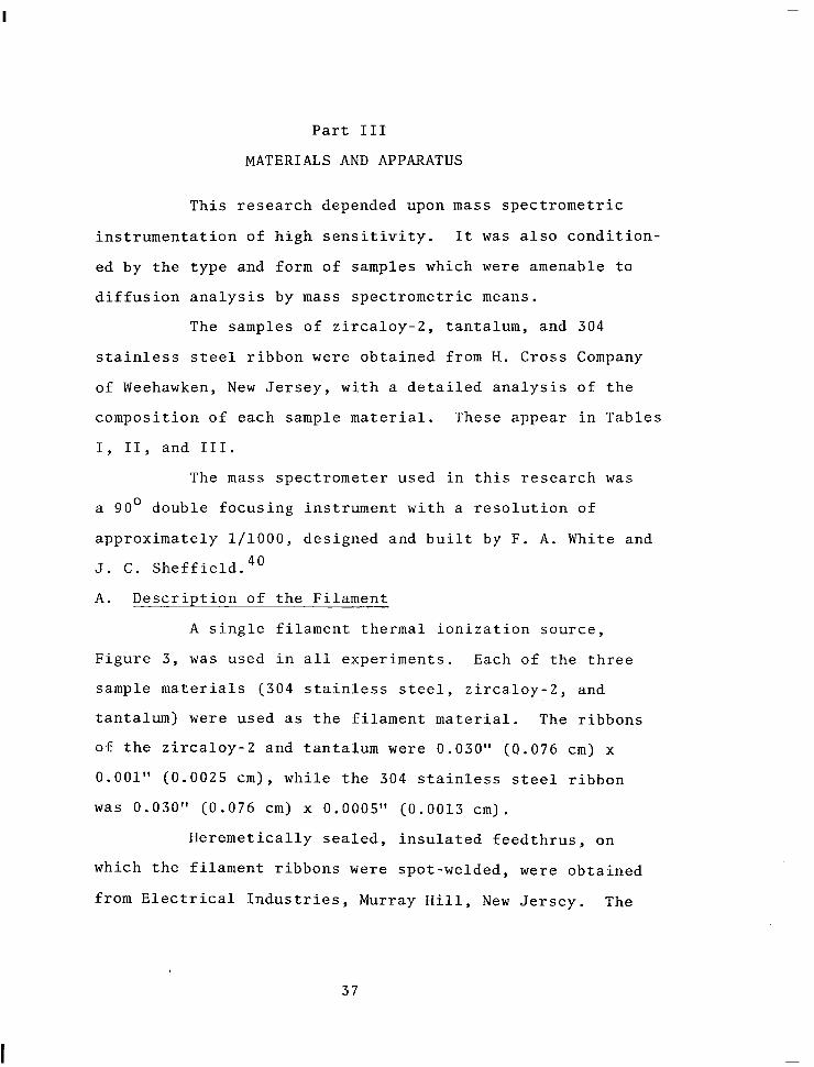
Part III
MATERIALS AND APPARATUS
This research depended upon mass spectrometric
instrumentation of high sensitivity. It was also condition-
ed by the type and form of samples which were amenable to
diffusion analysis by mass spectrometric means.
The samples of zircaloy-2, tantalum, and 304
stainless steel ribbon were obtained from H. Cross Company
of Weehawken, New Jersey, with a detailed analysis of the
composition of each sample material. These appear in Tables
I, 11, and III.
The mass spectrometer used in this research was
a 90' double focusing instrument with a resolution of
approximately l/1000, designed and built by F. A. White and
J. C. Sheffield.40
A. Description of the Filament
A single filament thermal ionization source,
Figure 3, was used in all experiments. Each of the three
sample materials (304 stainless steel, zircaloy-2, and
tantalum) were used as the filament material. The ribbons
of the zircaloy-2 and tantalum were 0.030" (0.076 cm) x
0.001" (0.0025 cm), while the 304 stainless steel ribbon
was 0.030" (0.076 cm) x 0.0005" (0.0013 cm).
Heremetically sealed, insulated feedthrus, on
which the filament ribbons were spot-welded, were obtained
from Electrical Industries, Murray Hill, New Jersey. The
37

Table I
COMPOSITION OF 304 STAINLESS STEEL
Carbon Manganese Phosphourus Sulphur Silicon Chromium Molybdenum Copper Nickel Cobalt
.056% 1.65 %
. 018%
. 012%
.49 % 18.53 %
. 31 %
.25 % 9.14 %
-03 %
38

I
Table II
COMPOSITION OF TANTALUM
TANTALUM
Ta Atomic Number 73 Atomic Weight 180.95 Crystal Structure BCC Melting Point OC 2996 Density gms/cc (2OOC) 16.6
Ibs./in3 0.600 MARZGRADE
MATERIALS ANALYSIS
Analysis: q Mass Spectmgraphic q Vacuum Fusion (Gases) 0 Emission Spectmgraphic II Conductometic (Carbon)
Element Content (ppm) Element Content (ppm)
0 < 5.0 s 2.0 C c 5.0 Cl 2.0 H < 5.0 K 0.1 N < 3.0 Ca 0.4 B c 0.1 < 0.1 F < 1.0 s: c 1.0 Na < 0.4 V 0.2 Mg -c 0.2 Cr 3.0 Al 0.5 Mn < 1.0 Si 0.7 Fe 100 P 0.3 Nl 1.0
METHOD OF PREPARATION: Electron Beam Zone Refined
STANDARD SINGLE CRYSTALS
cu
Zn Ge As Br Zr Nb MO
Ag Cd In
Content (ppmj Element
0.3 Sn c 0.1 Te < 0.4 I < 0.1 W c 1.0 Pt 4 1.0 AU
70.0 Pb < 0.5 Bi < 0.4 co < 0.3 All < 0.2 others
Content (ppm)
0.2 < 0.2 < 1.0
3.0 < 5.0 < 5.0 c 0.6 c 0.3 < 0.3
< 0.1
NOMINAL PURllY (TOTAJ-): 999%%
diameter S/in;, (1” Minimum Order)
w 96” $4” (.450”) $100. 5125. $150. $225.
Random Orientation. Oriented crystals. $75. additional orientation charge per crystal. independent of length. (100). (110). and (111) available.
SPECIAL APPUCAllON CRYSTALS
Cut from l/z” nominal diameter (elliptical cross-section) to approximately I/a” thickness, one face polished strain.free to expose specified crystallographic plane:
Within 1 o $65O./slice; additional slices of same orientation $200. each. Within 4O $325./slice; additional slices of Same orientation $150. each.
POLYCRYSTALLINE RODS
diameter in./lb. 137 H”
x0* 34 X” 15 p$” 8.5 1” 2.1 =-lb. on request.
Minimum Order: $50.00
gmsfin. 3.32
13.27 29.84
53 2.20
< 100 gms 100-300 gms 1-3 Ibs. Wgm Wgm S/lb. =-3 Ibs $3.00 $1.70
d- $550.
2.00 1.60 500. %e 1.85 1.55 475. 425. 1.75 1.45 450. 400. - 1.38 400. 350.
39

TABLE III
COMPOSITION OF ZIRCALOY-2
ZIRCALOY-2 INGOT HEAT NO. 387266
COMPOSITION IN PERCENT Top Bottom
Sn 1.45 1.48 Fe Cr Ni Zr
Al B 0.2 C 110 Cd <0.2 co (10 cu 16 H 7 Hf 41 0 1180 Mn <25 N 46 Si 73 Ti (25 IJ <25 LJ 1.5 v <25
0.15 0.16 0.11 0.11 0.05 0.06 BALANCE
IMPURITIES IN PPM 47 49
0.2 100
<0.2 <lo
15 <5 39
1150 <25
38 79
<25 (25 1.8 <25
INGOT HARDNESS, BHN Range 170 - 179 Average 176
40

SINGLE FILAMENT THERMAL IONIZATION SOURCE
FIGURE 3
41

feedthrus are designated as EI type A-40W-SS Mod H.
B. The Mass Spectrometer
The mass spectrometer separates chemical elements
according to their mass to charge ratio. The mass spectro-
meter shown in Figure 4 was used exclusively in this study.
A schematic of this two-stage, double focusing instrument
is shown in Figure 5. The major components of the instru-
ment include:
(a) Ion source (b) Electrostatic analyzer (c) Magnetic analyzer (d) Beam defining slit system (e) Ion detector and counting system (f) Vacuum system
Thermal Ionization. For mass spectrometric anal-
ysis, some method is needed to vaporize and ionize the sam-
ple into a beam of positively charged ions before entering
the electrostatic and magnetic filters. For the analysis of
metals, thermal ionization is an effective means of produc-
ing gaseous ions especially if the metal has a low ioniza-
tion potential compared to the filament's work function. As
the sample vaporizes, some atoms or molecules will leave the
surface of the filament with the loss of one or more of their
electrons. The hot filament surface has a higher affinity
for electrons than the metal itself. This is due in part,
to the intrinsic nature of the metallic crystal along with
the low binding energy of the outer shell electrons of most
metallic atoms.
42

.
P w
I .i
TWO-STAGE MASS SPECTROMETER
FIGURE 4

AMF’LlFIER/DISCRIhlINATOR / DRIVER
10.16 cm
h FINAL SLIT SYSTEM DATA ACQUISITION SYSTEM
ELECTRON MULTIPLIER Et BRIDGE CIRCUIT l5L/S VACION PUMP
MAGNETIC ANALYZER
50.8 CM. RADIUS OF CURVATURE
ION SOURCE
CENTER SLIT SYSTEM
DIFFUSION PUMP 75 L/S VAC ION PUMP
ELECTROSTATIC ANALYZER
50.8 CM. RADIUS OF CURVATURE
Two Stage, Double Focusing Mass Spectrometer
Figure 5
44

The probability of an atom evaporating from a sur-
face in the ionic state rather than as a neutral atom is
expressed by the relation,
+ n no
aE exp e+-+ a: eq ~~606TWP) (491
where n + is the number of positive ions, no is. the number of
neutral specie, e is the electron charge, IP is the ioniza-
tion potential of the sample in electron volts, 4 is the
surface work function of the filament material in electron
volts, k is Boltzmann's constant, and T is the surface
temperature in OK.
It can be seen that for elements where IP+ the
relative number of ions to neutrals produced will increase
with temperature.
Ions resulting from thermal ionization on the
filament surface are accelerated to high energy and defined
by collimating slits in the ion source. These high energy
ions pass through the electrostatic analyzer where they are
energy filtered. Ions with a discrete kinetic energy
(accelerating voltage) including a small energy spread
pass through the center defining aperture. The defining
slit determines the energy spread accepted. This filtered
heam of ions then enters the magnetic analyzer where the
beam is momentum filtered. Those ions of appropriate
energy and proper momentum (essentially mass) come to a
focus at the final slit and strike an electron multiplier.
45

Current pulses result from ion-electron conversion and sub-
sequent secondary electron amplification in the electron
multiplier tube. Output pulses are further amplified and
counted by an amplifier/discriminator/scalar system. Thus,
ions of the same mass are individually counted and the
exceedingly small ion currents can be quantitatively
measured.
By properly changing the accelerating potential
of the ion source, ions of other mass numbers are focused
on the electron multiplier. By comparing counting rates
for each mass position the isotopic ratio can be quantita-
tively determined.
46

Part IV
EXPERIMENTAL METHOD
A. General Experimental Techniques
From the literature, the most common method for ob-
taining diffusion coefficients is that of serial sectioning.
However, a mass spectrometric approach was chosen for this
work. The basic concept of the mass spectrometric technique
for determining diffusion coefficients is that a correlation
exists between the solute atoms moving through a solvent
lattice and the fraction of these atoms which are evaporated,
as ions, from the crystal surface at a given temperature.
In this work, a thin ribbon filament of solvent
material is used with its own impurity or solute concentra-
tion. No doping of the solvent was required and thus there
was no alteration of the crystal lattice. Since the mass
spectrometer source chamber pressure is well below the vapor
pressure of the solute material in the temperature range con-
sidered, the solute atoms diffuse to the filament surface,
and evaporate immediately. This results in a zero solute
concentration at the filament surface after the filament
temperature is raised to the desired level. Further, as the
ribbon thickness is much less than its length or width, the
diffusion problem may be considered to be one dimensional.
Application of Fick's Second Law for Diffusion
in a Thin Plate: Since the solute concentrations
47

under consideration are very small, the diffusion process
occurring in the ribbon may be described by
J(x,t) = -D aca(lt) ( so)
and
accx,t> = -Da2C(x,t) (51) at ax2
where J(x,t) is the solute flux, C(x,t) is the solute con-
centration, and D is the diffusion coefficient. For the
experimental conditions previously described, the solution
to Fick's second law for impurity evaporation from a thin
plate yields the solute concentration, as a function of
position in the filament and evaporation time,t.
Solving equation (51) by the method of separation
of variables, the solute concentration may be found to be
C(x,t) = ( A sin XX + B cos )ix ) exp (-X2Dt) (52)
2 where x = -(l/dT)(dT/dt) or -(l/X)(d2X/dx2), D is the dif-
fusion coefficient, t is time, and A and B are constants of
integration.
For solute depletion from a thin solvent plate with
an initial solute concentration f(x) across its thickness,
the boundary and initial conditions become
C = 0 at t 10, for x = h and x = 0
c= f(x) at t = 0, for h > x > 0
With these conditions, equation (52) becomes
C(x,t> = i C sin y ew I -Da2n2t 2 1 / f(x') sin nax' dx'
h h
(53)
48

Where h is the filament
law, equation (SO), the
surface ( x=0 ) becomes
thickness. Thus from Fick's first
solute atom flux at the filament
J(o,t) = (Z/h)c exp 1 -Dnhn*tj /f(x') sin nax dx' (54) h
or more conveniently, where n is an integer,
J(o,t> = A Z expl -Dn2n2t h2
I (55)
where A is a constant. For h2 < 16Dt the error in using
only the first term is less than l%pl
Positive Ion Emission from a Hot Metal Filament:
The combination of high temperature and solvent work function
causes a constant fraction of the evaporating solute atoms
to ionize at the filament surface at a given temperature.
According to the Langmuir-Saha equation, the ratio of the
number of emitted positive ions (n') to emitted neutrals (no)
is
n+/n' = B exp {( 4 - IP)/kT) (56)
where B is a proportionality constant, 9 is the filament
work function, IP is the ionization potential for the solute,
k is Boltzmann's constant, and T is the temperature of the
filament in degrees Kelvin.42
The mass spectrometer accelerates, mass analyzes,
and detects these emitted solute ions while excluding all
otherionic species from its detector. By combining
equations (54) and (55), and assuming that the atomic trans-
port time is greater than h2/16Dt, the time variation of the
49

detected ion current is
J(o,t> = A exp ( -rr2Dt/h2 ) . i57)
B. Experimental Procedures
The procedures used in this work are detailed
below to allow reproduction of the experiments. A general
procedure followed at all times was the wearing of lintless
gloves when handling anything going into the vacuum environ-
ment. The procedures described are:
1. 2.
43:
2: 7. 8.
1. Cleaning:
Cleaning Spotwelding Mass spectrometry Calibration of mass spectrometer Filament temperature measurement Data acquisition Treatment of data Error analysis
Filament holders: Clean metal surfaces with 4M HNOS, and rinse with de-ionized water. Dry under the infrared lamp.
Filament legs : Place in an alcohol bath immersed in the ultrasonic cleaner. Rinse with de-ionized water and dry under an infrared lamp.
2. Spotwelding:
By visual inspection, make sure electrodes are clean
Set to 18-25 watt-seconds
Place one end of filament next to the supporting legs and then spotweld
Do the same for the other end of the filament and leg
50

3. Mass Spectrometer:
Opening Source Region:
Close main gate valve, isolation valve, and the roughing valve
Open the foreline valve
Connect up nitrogen gas, turn on, and let it into the source chamber
Let chamber come to atmosphere, put clips on O-ring
Before dismantiling anything, make sure power is OFF
Screw filament assembly onto the top plate of the ion source.
Closing Source Section and Vacuum Pump Down:
Make sure no lint is on O-ring or glass, and then put glass back on
Turn nitrogen gas off and close inlet valve
Open roughing valve, let it run for a few minutes
Close roughing and open foreline valve
Turn on first ionization gauge
Make sure liquid nitrogen is in cold trap
Open up the diffusion pump valve, do this SLOWLY and watch pressure gauge
Turn on automatic ionization gauge
Opening System and Operation:
Open isolation valve to sysrqm, after chamber pressure has reached 5 x 10 torr
Set electron multiplier tube to -4500 volts
Close gate valve on multiplier tube's ion pump
Turn on polarity switch to minus, on the electro- static lens power supply
Turn on main power to mass bridge ( ion source voltage divider )
51

Turn voltage control on filament heater, adjust current control for the temperature setting
Turn up voltage to desired setting, CAREFULLY
Begin data acquisition
System Shut Down:
Turn all voltage settings OFF
Close isolation valve
Open ion pump to electron multiplier tube
Turn multiplier tube voltage to -500 volts
Close diffusion pump gate valve
Turn OFF all power
Note: Liquid nitrogen will evaporate away
4. Calibration of the Mass Spectrometer:
It is necessary to calibrate the mass spectrometer
before undertaking any experiments measuring diffusion coef-
ficients. Using equation
B2R2 = (144)'(mVa) (58)
where B is the magnetic field in gauss, R is the radius of
curvature (in cm.) of the magnetic analyzer, m is the mass
of the isotope of interest in amu., and Va is the accelerating
potential in volts, the appropriate magnetic field-accelerating
potential values for a given mass can be determined.
Since the alkali metal atoms were to be examined,
calibrations were made using filaments which had solutions of
either rubidium or cesium evaporated on them. Rubidium has
two naturally occurring isotopes, mass 85 and mass 87. De-
tection of one mass and calculation of the magnetic field
allowed the determination of the accelerating potential of
52

the other isotope with the same magnetic. field. In practice,
an accurate calibration requires many repetitive measurements.
Cesium-133 is the only stable isotope of cesium, and provides
an accurate determination of the magnetic field.
Ion implanted, as well as micro-pipetted filaments
of Cs-133 were also used for calibration purposes. The iden-
tical .method was followed.
5. Filament Temperature Measurement:
Using a precision optical pyrometer, filament
temperatures were determined by visually matching the color
of the filament with the color of a calibrated, resistively
heated wire within the pyrometer. It is accurate to
within f3'C.
6. Data Acquisition Procedure:
The mass spectrometer data was obtained as follows:
1. The sample filament was placed in the ion source and the source chamber prevsure was evacuated to a pressure of about 10 torr.
2. The source voltage was set at the accelerating potential of the desired diffusing isotope.
3. The filament was raised in temperature until ions were detected at the given accelerating potential. The filament temperature was then determined.
4. The ion emission rate as a function of time was monitored until a slowly decreasing emission rate was observed. The latter indicated that the maximum emission rate had occurred and the exponential decay portion predicted by diffusion theory, had been reached.
5. At this point, the ion current was recorded for one second every four seconds utilizing a frequency-period-counter which has an accuracy of *l count.
53

6. The procedure was repeated for successively higher temperatures.
7. Treatment of Data:
A graph of the natural logarithm of the impurity ion current (represented by counts per second) from a particular solvent lattice versus time, for each temperature was plotted
The slope of the " linear best fit" line through the data was calculated
The diffusion coefficient was then calculated by
( slope of the line )a( thickness of filament/a )2
= -D
A graph was made of the In D versus 104/T('K)
Utilizing a PDP 8/I computer, the linear best fit line to the data points was made. The y-intercept of this line is the frequency factor, D and was calculated by the computer. The correlg;ion co- efficient of the data to the line was also calculated.
The activation energy, Q, was determined by multi- plying the slope of the line from the line in the preceding steg by the Rydberg gas constant in units of kcal/mole/ K.
8. Error Analysis:
Programs were written to provide the linear best
fit line from a set of data points. The program also gave
the detree of fitness in the form of a correlation coefficient.
All error values were determined by calculating the product-
moment coefficient of correlation and using a 95% confidence
level. A final program was written to obtain the standard
deviation for the activation energies. These programs appear
in Appendix 1 and 2.
54

Part V
RESULTS AND DISCUSSION
Following the procedure previously indicated, graphs
of the In (alkali metal ion count rate) versus time were
obtained. Figure 6 is an example of how the ion count rate
varies with time. These superposed curves illustrate the
detection of singly charged, mass resolved ions at several
temperatures. The counting rates are relative, but most
experimental measurements were in the region of 10 -14 to
lo-l7 amperes, corresponding to counting rates of 10' to lo2
ions per second.
Tables IV, V, and VI show the experimental results
for the diffusion of the alkali metals in 304 stainless
steel, tantalum, and zircaloy-2. All five naturally occurring
alkali metals were found in tantalum and in 304 stainless
steel; however, lithium was not found in sufficient quan-
tities to determine its diffusion parameters in the zircaloy-2
sample.
Activation energy plots for these diffusion systems
are shown in Figures 7 thru 20. The frequency factor, Do,
and the activation energy, Q, were calculated from these
plots and are presented in Tables VII, VIII, and IX.
The data derived from the activation energy plots
can be applied to the metallurgy of the system. For example,
a sharp discontinuity can be attributed to an allotropic
phase change in the host material. Since pure zirconium has
55

Id5 DlFFUSlON THRU TYPE 304 STAINLESS STEEL
RUN NO. TEMP “C
I 903 2 968
1052 II I0
IO 1"."'...'..."....'.-.'1"."'. ' I .'..,-,“,"'.,."'I".'
TIME (5 SECOND INTERVALS )
DIFFUSION OF Rb IN TYPE 304 STAINLESS STEEL
FIGURE 6
56

T('K)
1080 1107 1152 1179 1289
1381 1439 1449
u-l 1462 4 1481
1490 1520
1033 1058 1107 1110 1140 1176 1190 1230 1230
1238 1289 1290
TABLE IV DIFFUSION COEFFICIENTS OF THE ALKALI METALS IN TANTALUM
Li-7
D(cm2,sec)- T('K) 4.52*10-' 5.o3*1o-g
1522
6.86*1o-g 1534
1.10*10-8 1570
1.91*10-8 1575 1605 1621 1650 1650 1669 1675 1721 1802
Na-23
1311 1330 1348 1377 1464 1466 1488 1490 1527
2.80*10-' 1610
2.10'10-g 1634
2.9o*1o-g 1661
3.27~lo-' 3.3o*1o-g 4.69*10-' 4.46*10-' 4.71*1o-g 6.39*10-' 5.97'101; 2.99-10 6.86-10;; 1.23.10m8 1.31~10-8 1.09.10
T('K)
1110 1145 1172 1199 1235 1247
1267 1300 1314 1342 1355 1383 1403 1422 1447
1050 1076 1083 1111 1133 1155
1167 1227 1261 1366
K-39 D(cm2,sec~- T('K)
1.24*10-' 2.18.10-'
1471
4.18*10-' 3.47*1o-g
1495
4.64*10-' 1497 1499
7.44*1o-g 1524 1529
2.o2*1o-g
2.04'10-'
1595 1577
2.51'10;!, 1616 1664
3.78elO-g 2.55*10mg 1672 1718
4.01.10 2.86*10mg 1745
4.36*10-' 4.11*1o-g 1767 1828
Rb-85
8.00*10-' 2.60*10-' 6.10*10-'
1372 1395
9.8040-' 1437
1.10~10-8 1443
1.6O*1O-8 1538 1560
5.20*10-'
6.30*10-' 5.4o*1o-g
1582 1616
7.80*10-' 1667 1695 1783 1789

T('K)
992 1040 1070 1082 1100 1122 1124 1133 1181
1178 1289 1316 1326 1366
TABLE IV CONCLUDED
cs-133 D(cm'/sec) T('K) 4.46.10-' 5.5os1o-g
1377
7.32*10-' 1393
9.58*10-' 7.96'10-'
1422
1.24*1O-8 1506 1543
1.03.10-8 1555
1.01~10-8 1600
1.38s1O-8 1623 1631
3.74*lo-g 8.42.10-' 5.19*1o-g
1650 1712 1745
D(an2/sec) 1.09*10-8 9.96.10-' 1.2o*1o-8 1.54.10;; 1.59dOm8 2.20010 1.58'10-8 2.14.10;; 1.75'10 1.61'1O-8 1.78.10;; 2.47'10
I

-
T(OK)
914 933 955 991
1013
1060 1075 1076 1091
: 1117 1121
TABLE DIFFUSION COEFFICIENTS OF THE
Na-23
D(cm2/sec) T(OK)
5.67*10-' 5.20*10-'
1135
1.10*10-8 1149
1.78010-~ 1157
1.88*10-8 1181 1185 1208 1229 1266
1326 1357
2.4X0-' 1366
V ALKALI METALS IN ZIRCALOY-2
K-39 T('K) D(cm2/sec~ T('K)
934 939 950 956 966 982 990 990
1002 1008 1013 1022 1026
1066 1073 1076 1083 1087 1096 1101 1111
1122 1127 1129 1133 1140 1145 1181 1183 1190 1205 1227 1248 1259 1272
1302 1323 1332 1340 1344 1361 1391
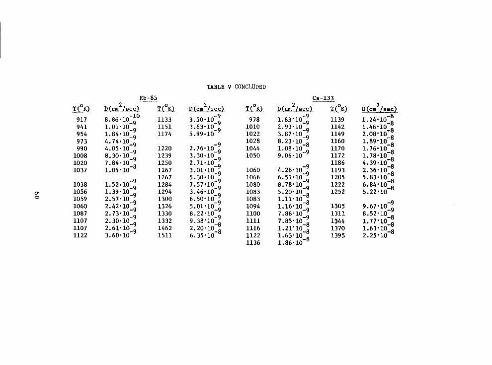
TABLE V CONCLUDED
o\ 0
T('K)
917 941 954 973 990
1008 1020 1037
1038 1056 1059 1060 1087 1107 1107 1122
Rb-85 D(m2/sec) T('K)
8.86*10-1° l.ol~lo-g 4.74*1o-g 1.84*10-'
1133 1151 1174
4.o5.1o-g 8.30*10-' 7.84.10-'
1220 1239
1.04.10-8 1250 1267
1.39.1o-g 1.52.10-'
1267
2.57.10-' 1284 1294
2.73.10-' 2.42*10-'
1300
2.61*10-' 2.30*10-'
1326 1330
3.60.10-' 1332 1462 1511
D (cm2/sec) T('K)
978 1010 1022 1028 1044 1050
1060 1066 1080 1083 1083 1094 1100 1111 1116 1122 1136
cs-133 D(m2/sec) T('K)
1.83'10-' 2.93*1o-g
1139
3.87*10-' 1142
8.23.10;; 1149 1160
9.06.10-' 1.08.10 1170 1172 1186 1193 1205 1222 1252
1305 1311 1344 1370 1395

T('K)
1140 1143 1156 1175 1186 1189 1220
948 983
1002 1044 1106 1122 1133 1149 1168
TABLE VI DIFFUSION COEFFICIENTS OF THE ALKALI METALS IN 304 STAINLESS STEEL
Li-7
D(cm2/sec) T('K)
1289 1316 1319 1340 1344 1368 1379 1427
Na-23
1208
1227 1239 1241 1272 1276 1326
T('K)
953 986
1008 1038 1040 1050 1062 1073 1075 1076 1109 1116
1043 1060 1065 1071 1080 1116 1127 1133 1155
K-39 D(m~~,sec)-T(~K~
1119 1134 1172 1175 1198 1215
1305 1330 1389 1433
Rb-85
1161 1176 1182 1198
1355 1404 1445
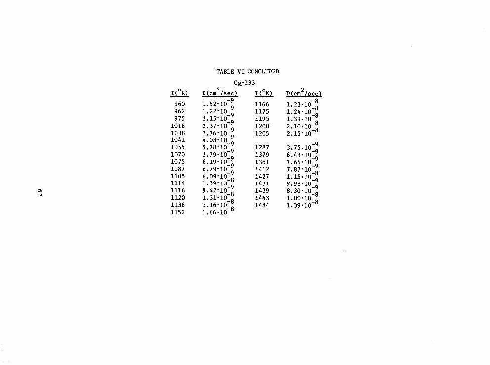
T(OK) 960 962 975
1016 1038 1041 1055 1070 1075 1087 1105 1114 1116 1120 1136 1152
TABLE VI CONCLUDED
cs-133
D(cm2/sec) T('K)
1166 1175 1195 1200 1205
1287 1379 1381 1412 1427 1431 1439 1443 1484
D(cm'/sec)

Table VII
Do and Q for IMPURITY DIFFUSION in 304 STAINLESS STEEL
Impurity
Li-7
Na-23
K-39
Rb-85
cs-133
928 < T('K) < 1228
DO ,Q
(1.86 * 2.01) x loo 52.96 * 0.54
(6.11 * 0.56) x 1O-7 14.22 f 0.19
(9.53 * 0.67) x 1O-7 14.09 f 0.15
(3.19 = 0.58) x 10 -1 41.92 * 0.38
(6.75 * 0.70) x 1o-4 25.04 * 0.22
Li-7
Na-23
K-39
Rb-85
cs-133
1228 < T('K) < 1789
(1.73 f 0.31) x lo5 84.42 f 0.56
(1.74 * 0.59) x lo4 74.08 f 0.93
(1.72 * 0.10) x lo3 75.22 * 0.18
(5.56 * 1.75) x lo6 98.16 * 1.01
(5.03 * 0.49) x 1o-5 24.50 * 0.26
Do is in units of cm2/sec
Q is in units of kcal/mole
63

Table VIII
Do and Q for IMPURITY DIFFUSION in TANTALUM
hpurity
Li-7
Na-23
K-39
Rb-85
cs-133
990 < .T('K) < 1230
DO Q
(5.15 * 0.91) x 1o-5 20.29 f 0.41
(2.07 * 0.27) x lO-(j 11.90 f 0.37
(2.71 * 0.50) x 1O-3 32.19 * 0.43
(1.22 f 0.37) x 10-l 36.46 * 0.72
(8.53 * 0.61) x lo+ 15.07 f 0.16
Li-7
Na-23
K-39
Rb-85
cs-133
1230 < T('K) < 1790
(3.38 * 0.35) x lo-' 25.49 * 0.32
(1.13 * 0.17) x 1o-6 15.46 * 0.47
(1.06 * 0.07) x lo-' 22.25 * 0.20
(2.33 * 0.24) x 1O-7 14.78 f 0.31
(1.18 * 0.12) x 10 -6 13.48 * 0.26
Dg is in units of cm2/sec
Q is in units of kcal/mole
64

Table IX
Do and Q for IMPURITY DIFFUSION in ZIRCALOY-2
900 < T('K) < 1045
Impurity DO Q
Na-23
K-39
Rb-85
cs-133
(9.76 * 2.99) x 1o-3
(2.12 * 0.31) x 1o-2
(1.11 * 0.26) x 101
(8.91 f 2.96) x lo2
1045 < T('K) < 1345
Na-23 (1.92 * 0.25) x 10-l
K-39 (3.08 * 0.41) x loo
Rb-85 (3.53 * 0.54) x 1o-4
cs-133 (7.74 * 1.01) x 1o-2
1345 < T('K) < 1520
Na-23 (5.46 * 0.75) x lOlo
K-39 (5.35 * 0.82) x 10'
Rb-85 (1.11 * 0.22) x 1o-2
cs-133 (1.21 * 0.30) x 1o-2
Do is in units of cm2/sec
Q is in units of kcal/mole
26.44 * 0.72
30.92 * 0.31
42.82 f: 0.55
52.91 * 0.79
40.77 * 0.37
46.10 f 0.38
25.79 f 0.44
35.03 * 0.37
116.19 f 3.48
111.06 * 0.58
37.59 * 0.75
36.74 f 0.94
65

1r7 ‘3 m I - - -
10-10 . . * . L . . a . . I 6,5 7nO 715 8,0 815 9,O CL5 1080 1085 1110
104/TtoK)
ACTIVATION ENERGY DIAGRAM OF NA-23 IN ZIRCALOY II
Figure 7

10-7 =g
0
10-8 E
8 \
Q\ q 7%
10-9 y
10-10 I I 4 . I I I . I . 9 I 1 1 I i 615 710 7,5 810 815 9,0 985 10,o 10,5 1100
ACTIVATION ENERGY DIAGWl OF: K-39 IN ZIRCALWII
Figure 8

- m - l
10-8 z I
&I - I I
\ - o\ 00 %
m jj@
10-g z - 0 - - -
10-10 1 . 1 I . 1 . . ’ I I I I I I I I I 6,5 7,O 785 880 8,5 9,O 985 1080 10,s LO
ACTIVATION ENERGY DIAGRAM OF: b-85 IN ZIRCALOY-II
Figure 9

10-10 ! . I . I I I I I I I I I 685 7’1’0 7,5 8,O 8,5 9,O 9,5 1010 1015 ll,o
ACTIVATION ENERGY DIAGR4’l OF Cs-I3 IN ZIRCALW-II
Figure 10

615 780 785 880 8,5 980 985
ACTIVATION ENERGY DIAGRAM tf h-7 IN 304 STAINLESS STEEL
Figure 11

10-7 7
10-8
8 \
7% 10-g
i
10-10 , I I I I I I I I
6,5 710 7,5 8,O 815 980 95 10,o 10,5 !
11,
ACTIVATION ENERGY DIAGRWl OF NA-23 IN 3CPi STAINLESS STEEL
Figure 12

10-7
10-8 1
10-10 l
I . I I I I I I I I I
685 700 715 8,O 8,5 9,o 985 1080 10,5
ACTIVATION ENERGY DIAGM ff K-39 IN 304 STAINLESS STEEL
Figure 13

10-10 J I I I I I I I I I I I
6,:5 780 785 810 885 910 985 1000 1015 l# / T(‘K>
ACTIVATION ENERGY DIAGR44 OF b-85 IN 304 STAINLESS STEEL
Figure 14

10-7 -3
d
10-8 1
id \
q P %
10-g 3 l
10-10 ' . I I I I I I I I I
605 710 715 810 885 900 915 1080 1015
ACTIVATION ENERGY DIAGRlM OF Cs-133 IN 3(w STAINLESS STEEL
Figure 15

10-8 -4 8 u-l \
7% 10-g
10-10 ! I I I I 5,O 585 1 610 6’45 7,O 785 8,O 8,5
1 910 9,s 10,o 10,5 1110
lI? / Tt”D
ACTIVATICXV ENERGY DIAGRAM CF LI-7 IN TANTAuRyl
Figure 16

10-10 510 5,5 610 615 700 715 8,O 815 910 915 1010 10,5 LO
l@ / T(‘K)
ACTIVATION ENERGY DIAGR4l -OF: N&3 IN TANTALUM
Figure 17
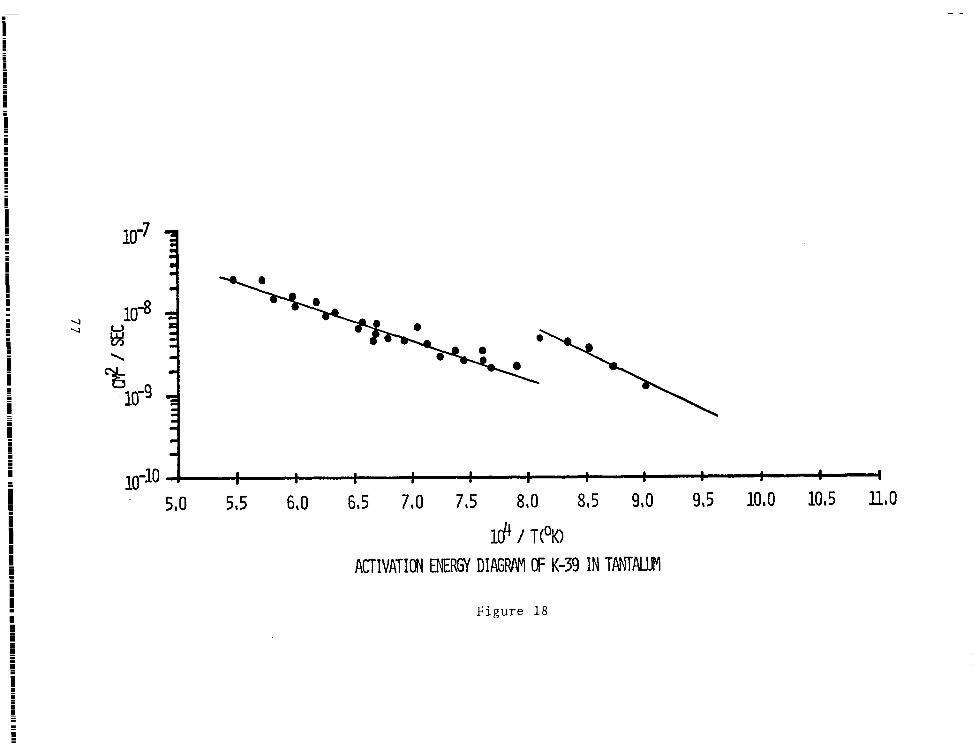
10-7 3 L m
0 I
v 10-8 0
= v bil \ -
73 L
10-g * =\
- 10-10 a I I I I I . . I 1 *
I * I I I I I I . I I
5,0 5,5 6,0 685 780 785 810 885 9,O 95 1010 10,5 1110
18 / T(‘K)
ACTIVATION ENERGY DIAGWI tF K-39 IN TPNTALUM
Figure 18

10-7
10-8 H
+I \ 03 %
10-g i
10-10 . 1 . I . I a . 1 . l I 1 . 4 580 515 610 6,5 7,0 7,5 8,O 8,5 9,0 9,5 1000 1015 IL0
l& / T(‘K>
ACTIVATION ENERGY DIAGRMI @ b-85 IN TPNTALUM
Figure 19

10-8 9
lo-lo I . . I
. . . .
l . I I .
510 515 600 685 7,O 785 880 8a5 910 915 1080 1015 LO
ACTIVATIMNERGY DIAGRPM ff Cd33 IN TPNTALUM
Figure 20

both a hexagonal close packed, h.c.p., and a body centered
cubic, b.c.c., geometry depending on the temperature, zir-
caloy-2, which has'a composition of %98.5% zirconium, will
probably have a h.c.p. and b.c.c. structure. However, in-
stead of having a single discontinuity, there is a large
transition region which possesses its own diffusion char-
acteristics. Pande, Naik, and Agarwala 43 have also observed
this three region activation energy diagram in their study
of the diffusion of chromium and iron in zircaloy-2. Their
transition region held limits of 780 and 980°C, while this
work extends the transition region from 772 to 1072'C. This
large transition region can be explained by a statistical
average of the diffusivity of both phases present at a par-
ticular temperature
When examining the stainless, steels, the results in
this work did not completely agree with literature values.
A reason for the discrepancy may involve the fact that the
composition of stainless steel has a wide range in the per-
cent abundance of its constituent elements. For example,
Delong 44 has found that 304 stainless steel changes from a
face centered cubic, f.c.c., to a body centered cubic, b.c.c.,
structure at 910°C, while the results in this study indicate
a phase change at 955'C.
While carbon, 45 deuterium and hydrogen, 46 molybdenum, 47
and sulpher 48 have been studied as they diffused through
tantalum the diffusion of the alkali metals have not been
studied in tantalum. Tantalum has a body centered cubic
80

structure, thus there will be no phase transformation. How-
ever, from the data obtained in this experiment it appears
that there has been a phenomenological occurence at approxi-
mately 1000°C. There have been many possible explanations
suggested, but the one that presents the greatest problem
in discounting it is that of cold working. For tantalum to
be processed into the thin ribbons used in this study, tan-
talum would undergo a great deal of cold working. It is
possible to remove these defects by annealing, and it so
happens that the annealing temperature for tantalum is 1000°C.
The resultant reduction in lattice disorder would tend to
decrease the diffusion coefficient. However, it would in- '
crease when the temperature was again increased. This is
exactly what occurs in figures 16 - 20.
These results provide an insight into the basic dif-
fusion mechanism in addition to supplying D, Do, and Q. For
example, the relationship between the diffusion coefficient,
D, and the ionic radius at a constant temperature can be
compared, by considering the alkali metal series; Li, Na, K,
Rb, and Cs, in the same host material. Plots of these five
impurity ions as observed in this study are -shown in Figure
21 for tantalum, Figure 22 for zircaloy-2, and Figure 23 for
304 stainless steel. Although there is no phenomenalogical
relationship, the diffusion coefficient versus mass is some-
what analoguous to sputtering yield data in which very large
differences in secondary ion yield vary with atomic mass and
ionic radius.
81
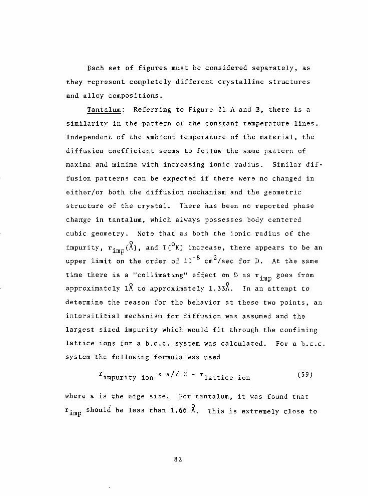
Each set of figures must be considered separately, as
they represent completely different crystalline structures
and alloy compositions.
Tantalum: Referring to Figure 21 A and B, there is a
similarity in the pattern of the constant temperature lines.
Independent of the ambient temperature of the material, the
diffusion coefficient seems to follow the same pattern of
maxima and minima with increasing ionic radius. Similar dif-
fusion patterns can be expected if there were no changed in
either/or both the diffusion mechanism and the geometric
structure of the crystal. There has been no reported phase
change in tantalum, which always possesses body centered
cubic geometry. Note that as both the ionic radius of the
impurity, 'imp Ci) 9 and T('K) increase, there appears to be an
upper limit on the order of 10 -8 cm'/sec for D. At the same
time there is a "collimating" effect on D as r. =mp
goes from
approximately 18 to approximately 1.33X. In an attempt to
determine the reason for the behavior at these two points, an
intersititial mechanism for diffusion was assumed and the
largest sized impurity which would fit through the confining
lattice ions for a b.c.c. system was calculated. For a b.c.c.
system the following formula was used
r. impurity ion <a/a-r lattice ion (59)
where a is the edge size. For tantalum, it was found that
rimp should be less than 1.66 1. This is extremely close to
82

1O-6 0-B
10-7 -
D 10-8 -
lo-9 - 1255
10-10 I . I . , . 1 . a I . . . . . * . . . . . ..I ,‘#‘I,., ‘.I. ,,
0,5 LO la5
lO-6 -A
10-7 -
D lO-* -
10-g -
lo-lo 1 m . . . I . . . I I I I.. . . I I , I . , I I I , . . . m l . l l 1
on5 LO L5
=imp
DtChSECI vs =,,,(fb AT CONSTANT T<% IN TANTALUM
Figure 21
83

the 1.67 1 point on the graph for the Cs+ ion. This implies
that the lattice structure of the host material plays a role
in limiting the size of the impurity ion's diffusion. To
go beyond this size would require additional energy. The
region of 1 < r imp (‘1 < 1.33 shows what might be considered
inhibited diffusion. This could be caused by the simultane-
ous diffusion of all the other impurities in this dynamic
system while being analyzed for just one particular impurity.
Zircaloy-2: A very interesting pattern of diffusion
can be observed in Figures 22 A, B, and C. Using the 900'K
line in Fig. 22 A as a reference, in a h.c.p. structure, as
the ionic radius of the impurity increases, the diffusion co-
efficient decreases. However, as the temperature is increased
it is evident that the lattice vibrations cause D to increase
and the larger impurity ions to diffuse at a greater rate.
This increase in acceptable ionic radius appears to have an
upper limit of about 1.47 8 which corresponds closely to the
radius of the Rb+ ion.
Figure 22 B represents the transition region where
the crystal structure changes from h.c.p. to b.c.c.. This
graph is not simply understood as the crystal structure
changes with temperature. It does appear that the disorder
induced in the crystal by the phase change increases the
probability of diffusion.
Figure 22 C shows the zircaloy-2 system in its b.c.c.
state. Note that D(125Q°K) is less than D(lQ40'K) even though
the temperature has been increased into the higher temperature
84

phase region. A possible mechanism to qualitatively explain
this sudden drop in diffusion rate is that as the transition
region is approached from a lower temperature, lattice defects
begin to occur before the transition point is actually reached.
These lattice defects are greatly multiplied in number i-n
the phase transition region due to the increased disorder
in the lattice structure. This increases the impurity dif-
fusion rate in the phase transition region. However, once
the phase transition is passed, the crystal lattice became
more ordered, and many of the lattice defects retreat to
defect "sinks," such as grain boundaries. This results in
an initial decrease in the diffusion rate. As the defect
sinks will release these defects into the crystal lattice
as the temperature increases, the diffusion rate will again
begin to increase.
Figure 22 C shows an interesting occurrence as both
T('K) and r. imp(') increase. In the region r. w > 1.47 x, D
is not only relatively invariant as r. imp increases, but also
relatively invariant as the temperature increases. It seems
that as T increases D is constrained to be of the order of
magnitude of 10m8 cm'/sec. A partial explanation is proposed:
if it is assumed that the solute will diffuse by an inter-
stitial mechanism, a relationship for the largest impurity
ion accepted before configuration problems are encountered
is again equation (59). Using rlattice ion of zirconium, it
is determined that r- =mp < 1.47 El. From rimp = 1.47 Al in
Figure 22C, the diffusion coefficient changes very little
85

Ia5 -C
Id6 - NA+ I(’ RB+ cs+
1500 +----A. Id7 1450 - -
lci9 1300 * -
1250 . Id0 I I I I I 1 1 I
.5
Iti * 1 1040
HY8 - ‘tg :\.A----+
n lG9 - +=z 90o .\::q:
,(jlO - ‘1. I I I 1 1 ’ ’ ’ ’ I 1 I I I 1 , I
.5 I!0 1.5
r. =mP
DKlih vs rimp& AT CONSTANT T(‘K) IN ZIRCALOY-II
Figure 22
86

with increasing r. imp' Even increasing the temperature does
not cause much of an increase in D after r. imp reaches 1.47 !.
The changing behavior of D in the range of 1.33
<r imp (‘1 < 1.47 could possibly be explained by the fact that
the zircaloy-2 has a certain percentage (~1.5) of tin, which
has an ionic radius of 0.93 i. This means that for a given dif-
fusion jump through four restraining lattice ions, if one is
a tin ion, impurity ions of larger size will be able to dif-
fuse through easier than if all four lattice ions were zir-
conium. This would represent only a minor perturbation as
the amount of tin is limited. At higher temperatures, this
represents a negligible effect as r. imp gets closer to 1.47 X
the size plays an increasingly inhibiting effect.
304 Stainless Steel: Stainless steel 304 presents a
special challenge for determining diffusion parameters using
a mass spectrometer. No longer is just a pure metal being
considered, as in the case with tantalum, or a very dilute
alloy as with zircaloy-2, but an alloy which has major con-
stituents of iron, nickel and chromium. The activation energy
plots have shown the phase change representing a transforma-
tion from f.c.c. to b.c.c. along with the corresponding
activation energies. On the other hand, Figures 23 A and B
represent a more complex picture in regard to D as both, r.
and T are varied. =w
Figure 23 A represents the f.c.c. structure of the
stainless steel. As each succeeding temperature line is
examined, a pattern in the region of approximately 0.70 R
87

and 1.5 w takes place with an apparent change of slope and
vortex, respectively. This can be explained by the fact that
as the temperature is increased the lattice vibrations are
increased so that it is easier for the impurity of a larger
size to diffuse. There is a limit as to the size that will
be accommodated. This is primarily controlled by the crystal-
lographic structure of the host lattice. Stainless steel is
affected in that there may be unit cells of different host
ions, representing the major constituents of stainless steel,
and grain boundaries may differ for specific samples. When
the effect of Ni in the f.c.c. structure is considered r- Imp should be less than 1.07 Al. Configurational limitations do
not appear to be significant until r. =mP
is approximately
1.30 x and that the region from 1.0 Al to 1.3 R is a relatively
temperature and radius independent region. When r. imp
becomes
greater than 1.33 ?L, the larger size ion cannot diffuse as
readily until more energy is supplied to increase the lattice
vibrations.
Figure 23 B represents the b.c.c. structure of 304
stainless steel where there are again inflection points
which indicate an area of physical constraints. The point
~1 i is caused by the influence of Ni , while the area around
1.3 i is caused by the influence of Cr (r
than 1.23 %) and Fe imp should be less
(r imp should be less than 1.34 i).
After r- =mp becomes greater than 1.33 x, D drops unless more
88

lO-4 1 B
D lO-6
10-7
10-8
10-g
lo-lo
lO-7 - A
lo-* - 1283 1255 D 1o-g 1200 - 1172 1141
lo-lo -' 1089 1033 1000
104 - ; ; -..; ; : gl" ;' : ; ; ; ; ; : ; ; ; )
005 LO 105 'imp
DKih vs =,,d) AT CONSTANT T<'D IN 302 STAINLESS STEEL
Figure 23
89

energy is given to increase the lattice vibrations. There
appears to be a significant size effect at approximately .1.67 2.
The increase in D at lower temperatures is probably due to the
fact that there are unit cells consisting of different sized
lattice ions, so that larger ions than normal could diffuse
through. However, this is a limited effect as T increases, the
increased lattice vibrations no longer tend to increase D and
the larger size of the impurity ion becomes a more dominant
parameter.
In fact, there are two aspects to note. The first is
that along with the other samples, as both r. w and T increase
it appears there may be an upper limit for impurity diffusion
coefficients in these b.c.c. structures of approximately
lo-8 cm'/sec. The second is that as in the case of zircaloy-2,
after the phase change the diffusion coefficient drops
initially and then proceeds to rise with temperature.
As there are no reported values for the diffusion of the
alkali metals in 304 stainless steel, it was thought that a com-
parison between Na-23 and C-14 diffusion in 304 and 316
stainless steel would be desirable. This would enable one to
determine whether the results obtained via mass spectrometry
were reasonable in comparison to the determination of diffusion
coefficients by other methods for a different element. Table X
illustrates that the Na-23 diffusion is within an order of
magnitude of the diffusion of C-14. The Na-23 also seems to
diffuse at a slower rate than the C-14 as would be expected
since the Na-23 has a larger ionic radius than c-14. The C-14
diffusion coefficients were determined by Perkins and Carlson, 49
90
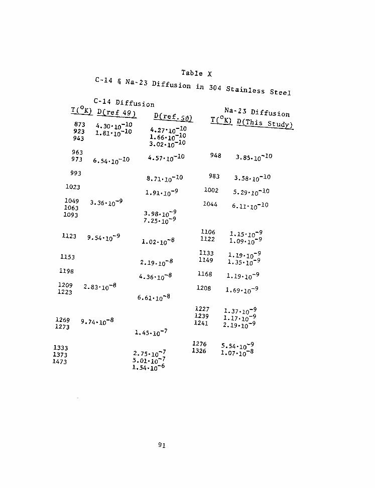
Table X C-14 6 Na-23 Diffusion in 304 St
ainless Steel
C-14 Diffusion J('K) D(ref 49)
D&f. so) Na-23 Diffusion
T('K) D(This Study) 873 923 943
963 973 6.54-10'lo
I”:,‘,‘:$
3.02qO-10
4.57qo'10 948 3.85.10-10
983 3.58qO-10 993
1023
1049 1063
3.36~10'~
1093
1123 9.54*10-9
1153
1198
1209 1223
2.83qO-8
1269 1273
9.74*10+
1333 1373 1473
8.71qO-10
1.91*10-9
3.98.lo-' 7.25qO-g
1.02.10-8
6.61*10'8
1.45.10-7
1002 5.29*10-10
1044 6.11qO-10
1106 1122
1133 1149
1168
1208
1.19.10-9
1.69.10"
1227 1239 1241
1276 1326
1.37.10-9 1.17.10-9 2.19*10-9
5.54.10-9 1.07910'8
91

and by Agarwala, Naik, Anand, and Paul. 50
In the further analysis of the data, two additional
relationships merit examination. Based on equation (48)
D= Do exp (-Q/RT)
it would seem that there should be some type of direct re-
lationship between Do and Q. Using the PDP 8/I computer a
best fit least squares program was run utilizing data on Do
and Q for h.c.p., f.c.c., and b.c.c. structures and at all
temperatures. It was found that the correlation coefficient
for the best fit line was 0.98 where 1.0 is a perfect fit.
Subsequently, it was determined that the relation between Do
and Q was
DO = 3.3 x lo-8 exp {(0.36)(Q)) . (60)
Whether or not this equation applies only to a dilute solute
diffusion of the alkali metals in these particular matrices,
or for any other diffusing system requires further investiga-
tion.
A second interesting consequence of this work involves
the possibility of using this method to further develop
concepts on ultra-fast diffusion. Ultra-fast diffusion
has been considered when the solute diffusion is much greater
than self-diffusion in the host material. An example is the
diffusion analysis of zircaloy-2 in this work. The self-dif-
fusion rates of pure a-zirconium have been determined by
Dyment and Libanati. 51 For a temperature range of 1036'K to
1130°K, they found D to be on the order of lo-l2 to lo-l3
cm‘/sec, while in this study, the diffusion rates of the alkali
92

metals for the same temperature range were on the order of
lo-8 to 10 -9 cm2/sec. This is approximately four to five
orders of magnitude faster. Ultra-fast diffusion has been
suggested by Hood and Schultz 52 to take place by an inter-
stitial mechanism. They studied both Co-60 and Fe-59 dif-
fusion in pure a-zirconium and found that D was of the order
of 10 -7 to 10 -9 cm2/sec which corresponds well with this
work. That ultra-fast diffusion would take place by an
interstitial mechanism coincides with the mechanism for de-
termining the largest diffusing ion size; a concept used to
explain figures 22 and 23.
It should be further noted that in Part II, con-
cepts of the jump frequency w, the mean vibrational frequency,
v , and the change in free energy, AG, were all discussed.
With the results obtained in this study, it now becomes im-
portant to determine some of these quantities.
Zener3' has stated that while it would not be
impossible for AG to increase with increasing temperature,
it would be highly improbable. The reason for this is that
a negative temperature coefficient of the elastic moduli
exists. Zener also found that the change in entropy, AS
can be related to the activation energy, Q, by
As = x BQ/T, I 611
where x is a numerical coefficient essentially equal to
93

unity for interstitial, B is a dimensionless quantity tabu-
lated by Zener for some pure metals, and Tm.is the melting
temperature for the host material. The value of AS can be
used to calculate v using
DO = (l/6) ai v exp (AS/R) (62 1
provided that Do is known.
Of the three sample materials used in this study,
B has been determined for tantalum only. It has a value of
0.40. Using values for Do obtained experimentally, v can be
determined. Once the values of v have been determined, w
can be calculated using equation (23).
w = vN m = v exp (-Q/RT) exp (AS/R)
Table XI gives the calculated values for w for the five
diffusing impurity isotopes in both temperature regimes.
94

Table XI
Calculated Values of v and w For Tantalum
990 < T(.'K) < 12'30
Jmpurity v (set -1 ) exp(-Q/RT) e-xp(AS/R) w (set -3
Li-7
Na-23
K- 39
Rb-85
cs-133
Li-7
Na-23
K-39
Rb-85
cs-133
2.83 x 10¹¹ .997 1.001
1.14 x 1o1O .998 1.0007
1.49 x 10¹³ .995 1.002
6.71 x 10¹⁴ .994 1.002
4.69 x lOlo .998 1.001
1230 < T('K) < 1790
1.86 x loll .996 1.002
6.22 x 10' .998 1.001
5.83 x lOlo .997 1.001
1.28 x 10' .998 1.001
6.50 x 10' .998 1.001
2.82 x 10¹¹
1.13 x 1o1O
1.48 x 10¹³
6.68 x 10¹⁴
4.68 x lOlo
1.85 x 10¹¹
6.21 x 10'
5.82 x lOlo
1.27 x 10'
6.49 x 10'
95

Part VI
CONCLUSIONS
It was the purpose of this work to illustrate a new
technique in the general field of materials characterization.
The transport of impurities, in the p.p.m. to p.p.b. range
and less, is becoming increasingly important. Since the
mass spectrometer is an instrument which can detect impurity
concentrations on this scale, it offers another view of the
high temperature diffusion properties in materials which are
of engineering usefulness. This is instead of being confined
to the world of the single crystal.
As a consequence of this work, not only were the dif-
fusion coefficients of the alkali metals in the sample
materials calculated, but known phase transformations were
determined in the samples of 304 stainless steel and zircaloy-
2. This, of course, lends a measure of credibility to the
results obtained.
While the primary intent of this work has been accom-
plished, it has been shown that what used to be a chemists
tool can be applied in metallurgical research. It is not
to be suggested that the mass spectrometer is the ultimate
instrument, but rather that it allows one more unique way of
looking at material's properties on the atomistic level. It
is conceivable that by determining the relationship between
the diffusion coefficient and the atomic radius of all the
impurities in a material that a better understanding of
diffusion processes could be obtained. It is hoped that
96

further funding will allow this laboratory to pursue this
and to see how ion implantation of selected species affect
the diffusion process in certain materials - i.e., semi-
conductors.
97

APPENDIX
98

APPENDIX 1
Program to Determine Least Squares Fit of Data to Exponential Curve, Correlation Coefficient,
and 95% Confidence Limit
C-8K FOCAL @I 969
~1.10 T !!r “THIS PROGRAM FITS PAIRS OF POINTS TO AN EXPONENTIAL PI.11 T !“LEAST SQUARES CURVE FIT - TO THE EQUATION: Y=A+EXP(S*\) 01 .I2 T !” x IS THE RECTANGIJLAH ARSYSSA Q1.13 T !” Y IS THE RECTANGULAR ORDINATE (INTERNAL CONVERSIOFJ TO LOG?’ @I .I4 T !” A IS THE Y-INTERCEPT 01.15 T !” B IS THE SLOPE ON SEMI -LO6 PAPER 01.16 T !” R IS THE CORRELATION COSFFICIENT 01.17 T !” CL IS THE 95% CONFIDENCE LIMIT +I- AT X=(TEST POINT) WI. 18 T ! !“PRoGRAM OPERA1 IoN: 131.19 T !” AFTER FIRST PROMPi ENTER ‘THE NUMBER OF ORDERED PA IRS 01.20 I !” THEN -ENTER X 8 Y AS t?EQUESTED BY THE PROGRAM 01.21 T !” -ENTER T(0.bj25) FOR THE SPECIFIED D.F. WHEN REQUESTED 01.22 T ! ** -ENCER THE NlJMBER OF TEST POINTS 01.23 T !” -ENTER THE TEST POINTS 01 .3O A ! ! !“ENTER THE NUMBER OF VALUES: “N 01.35 S SX=@;S SY=B;S %T=D;S XY=(?;S YT=O 01.40 I (N-1) 9.9~1.6 81.50 F I=1 rN;D 2 01.55 G 3.1 01.60 T !“TRY AGAIN -- 1 IS NO GOOD 01.65 G 1.3
02.10 A !“ENTER X: “X,“ENTER ‘Y: “rY:S Y=FLOG(YI 02.15 S S%=Sx+x;S SY=SY+r;S XT=xT+Kr2;S Xr=XY+x+f;S YT=YT+Yt2
03.10 s 03.15 T 93.20 S 03.30 s 03.40 s 03.50 s 03.55 s 03.60 C 03.65 S 03.70 c 03.75 s 03.80 C 03.85 s 03.30 G
XS=SX/N;S YS=SY/N !!“THE AVERAGE VALUE OF X IS: “,t,XB Yy=YT- (SYt2/N) xX=~T-(Sx?2/N) lT=XY-(Sy*SX/N) SS=<TTt2 )/XX +lS=(YY-5S,/(N-2, CALCULATION OF THE SLOPE -- 0 B=TT/x? CALCULATION OF THE Y-INTERCEPT -- A A=FExP<Y$-9*X$) CALCULATION OF THE CORRELATION COEFFICIENT -- R H=TT/FSOTCXX*YY) 5.10
99

W.lO C PRINT OUT THE RESULTS 04.20 T 2, ! ! !“RESULTS: Q4.30 ‘7 !” THE SLOPE IS: “,B 04.40 i !‘* THE Y-INTERCEPT 1.5: “,A 04.50 T !,” THE CORRELATION COEFFICIENT IS: “,I? 04.60 R 04.70 T !!! !“IF YOU WISH TO STOP -- AT THE NEXT PROMPJ TYPE c-1) QLI.SQ T !” OTHERWISE CONTINUE 04.90 G 1.3
OS.18 C INPUT FOR THE DETERMINATION OF THE 95% C.L.‘S FOR EACH TEST PT OS.15 T a2.0 B! !“ENTER THE VALUE OF T(0.025, FOR “,/V-2, ” DEGREES 05.16 A ” OF FREEDOM: “rDF 05.20 A !“ENTER THE NUMBER OF TEST POINTS: “,M 85.25 F I=l,M:D 6 05.30 DO 4 05.35 F I=l,w:S CL(I)=DF*FSGT<MS*(I/N+(x(I)-~)t2/~~)) 05.36 F 1=1,w;S Y(I)=FEXP<B+X(I))fA 05.37 F I=I,M;D 7 05.36 D 9.04 05.39 0 9.05 05.40 F I=ltM;D 9.1 05.45 G 4.70
06.05 C INPUT OF TEST POINTS -- X(w) 06.10 T 22. 0, !“ENTER TEST POINT X(“,J,“): ” 06.20 A K(I)
07.10 S ZA=F&X~(FLOG(Y(I))+CL(I)> 87.2U S ZR=FEXP(FLOG(Y ( I) )-Cl-( I)) 07.30 S ZC(I)=FkBS(ZR-ZR)/2
09.04 T !!“TEST POINTS fiND THEIR RESPECTIVE 95% C.L.‘S 09.05 T ! !” M 1. ,“K<M) Y’(M) 09.10 7 !,%2.0,1,%,” “#XC I),” “rY(I>,” “rZC(I) OS.90 T !“THE END”;G *~@~~~C?@gk?Ci
CL8
100

APPENDIX 2
Program to Determine D for a Given Temperature Provided Do and Q are Supplied
C-8K FOCAL @ 1969
01.01 C PROGRAM: DIFF 01.02 c 01 .I0 A ! ! !“WHAT IS THE SAMPLE MATERIAL? “,A 01.20 A !“bJHAT IS THE DIFFUSING ISOTOPE? “,A,B 01.30 A !“WHAT IS THE TEMPERATURE RANGE? “rAr”T0 “rBr”DEGREES KELVIN.” 01.35 A !“WHAT IS THE VALUE OF D(0)? “DO 01.40 A !“WHAT IS THE VALUE OF THE ACTIVATION ENERGY? “Q 01.60 T !r”,
02.10 A !“T= *‘,T 02.15 I (T) 2.6r2.5 02.20 S D=DB*FEXP(-Q/C2E-3)*T) 02.25 G 3.1 02.30 T ” II , “D= “D
02.31 G 2.1 02.35 T ” II ,“D= “0 02.40 G 2.1 02.50 G 1.1 02.60 T !!!!;Q
03.10 I <1000-T12.3r2.3n2.35 *
101

REFERENCES
1.
2.
3.
4.
5.
6.
7.
8.
9.
10.
11.
12.
13.
14.
15.
16.
17.
18.
Fick, A., - Ann. &. Lpz., 170, 59, 1855.
Fourier, J., Theorie Analytique de Chaleur, Oevures de Fourier, 1822.
Davidson, B., "Neutron Transport Theiry," Oxford University Press, London, p. 16, 1957.
Boltzmann, L., Ann. Phys., 53, 960, 1894.
Matano, C., Japan. Phys., 8, 109, 1938.
Gertsriken, S. D. and I. Y. Dekhtyar, "Solid State Diffusion in Metals and Alloys," AEC-tr-6313, USAEC Division of Technical Information, Washington, D. C., 1964.
Willard, N. H., L. L. Merritt, Jr., and J. A. Dean, "Instrumental Methods of Analysis," Fourth Edition, D. Van Nostrand, New York, p. 210, 1965.
McCracken, J. M. and H. M. Love, Phys. Rev. Letters, 5, 201, 1960.
Walling, J. D., Doctor of Philosophy Thesis, R.P.I., June, 1973.
Shewmon, P. G., "Diffusion in Solids," McGraw-Hill, New York, 1963.
Cottrell, A. H., "An Introduction to Metallurgy," Edward Arnold Ltd., London, 1967.
Askill, John, "Tracer Diffusion Data for Metals, Alloys and Simple Oxides," 1970.
IFI/Plenum Data Corp., New York,
Shewmon, op cit., p. 7.
Walling, op cit., p. 35.
Compaan, K. and Y. Haven, Trans. Faraday Sot., 52, 786, 1956.
Dekker, A. J., "Solid State Physics," Prentice-Hall, Englewood Cliffs, New Jersey, 1959.
Shewmon, op cit., p. 56.
Shewmon, op cit., p. 56.
102
----. ---- _._..._. . . . . . . . ..a-.., . . . . ,a-.. .,, , . .,, ,,,

19.
20.
21.
22.
23.
24.
25.
26.
27.
28.
29.
30.
31.
32.
33.
34.
35.
36.
37.
38.
39.
40.
41.
42.
Dekker, op cit., pgs. 65-67.
Dekker, op cit., p. 62
Zener, C., "Imperfections in Nearly Perfect Crystals," Wiley, New York, p. 287, 1952.
Dekker, op cit., p. 62.
Shewmon, op cit., p. 60.
Huntington, H. and P. Ghate, Phys. Rev. Letters, 8, 421, 1962.
Shewmon, op cit., p. 110.
Shewmon, op cit., p. 97.
Swalin, R., Acta Met., 5, 443, 1951. - Overhauser, R. A., Phys. Rev., 90, 393, 1953.
Reiss, H., Phys. Rev., 113, 1445, 1959.
Feit, Michael; Phys. Rev. B.; 3, 1223, 1971.
Feit, Michael; Phys. Rev. B; 5, 2145, 1972.
Huntington, H. B., and F. Seitz; Phys. Rev; 61, 315, 1942.
Lazarus, David; phys. Rev; 93, 973, 1954.
Johnson, R. P.; Phys. Rev; 56, 814, 1939.
Zener, C.; Acta Cryst; 3, 346, 1950.
LeClaire, A. D.; Acta Metal; 1, 438, 1953. -- Wert, C. and C. Zener; Phys. Rev; 76, 1169, 1949.
Turnbull, D. and R. E. Hoffman; Acta Metal.; 7, 407, 1959.
Zener, C; J. Applied Phys; 22, 372, 1951.
White, F. A., and J. C. Sheffield, Knolls Atomic Power Laboratory Report, KAPL-873 (1952).
Schwegler, Jr., E. C., Doctor of Engineering Thesis, R.P.I., August 1967.
Langmuir, I. and K. H. Kingdon, Proc. Roy. Sot. (London), A 197, pgs. 61-79, 1925.
103

43. Pande, B. M., M. C. Naik, and R. P. Agarwala, J. of Nut. Mat., 28, 324, 1968.
44. Delong, W. T., We'lding Journel, p. 274, July, 1974.
45. Son, R., M. Miyake, and T. Sano, Tech. Rep. Osaka. Univ., 18, 317, 1968.
46. Zuchner, H., and E. Wicke, Z. Phys. Chem. N.F., 67, 154, 1969.
47. Borisov, E. V., P. L. Gruzin and S. V. Zemskii, Zosch. Pokvy. Metal., 2, 104, 1968.
48. Vandyshev, B. A. and A. S. Panoj, Izv. Akad. Nauk, SSSR Metal, 1, 244, 1969.
49. Perkins, R. A. and P. T. Carlson, Metal. Trans., 5, 1511, 1974.
50. Agarwala, R. P., M. C. Naik, M. S. Anand, and A. R. Paul, J. of Nut. Ms., 36, 41, 1970.
51. Dyment, F. and C. M. Libanati, J. of Mat. Sci., 3, 349, 1968.
52. Hood, G. M. and R. J. Schultz, Phil. Mag., 1972.
104

1. Report No. 2. Government Accession No.
NASA CR-31 65 4. Title and Subtitle
DIFFUSION AND PHASE CHANGE CHARACTERIZATION BY MASS SPECTROMETRY
7. Author(s)
Mark E. Koslin and Frederick A. White
9. Performing Organization Name and Address
Rensselaer Polytechnic Institute Troy, New York 12181
12. Sponsoring Agency Name and Address
National Aeronautics and Space Administration Washington, DC 20546
3. Recipient’s Cat&q No.
j%
8. Performing Orqamzation Report No.
10. Work Unit No.
11. Contract or Grant No.
NSG-1360
13. Type of Report and Period Covered
Contractor Report
14. Sponsoring Agency Code
15. Supplementary Notes
Langley Technical Monitor: George M. Wood, Jr.
Final Report
16. Abstract
This report focuses on the high temperature diffusion of trace elements in metals and alloys. Specifically, these measurements have been made by high sensi- tivity mass spectrometry in which individual atoms were detected, and quantitative data was obtained for zircaloy-II, 304 stainless steel, and tantalum. Additionally, a mass spectrometer was also an analytical tool for determining an allotropic phase change for stainless steel at 955'C, and a phase transition region between 772OC and 1072oC existing for zircaloy-II.
Diffusion rates were measured in thin (0.001" (0.0025 cm) and 0.0005" (0.0013 cm)) ribbons which were designed as high temperature thermal ion sources, with the alkali metals as naturally occurring impurities. In the temperature and pressure regime where diffusion measurements were made, the solute atoms evaporated from the ribbon filaments when the impurities diffused to the surface, with a frac- tion-of these impurity atoms ionized according to the Langmuir-Saha relation.
While these measurements were made on only a few important materials, the techniques developed can be clearly applied to many other alloys important to space vehicles and supersonic transports; and, with appropriate modifications, to the diffusion of impurities in composites.
7. Key Words (Suggested by Author(r) I
Mass spectrometry Trace elements
__-- ._. -- .._. _i_+_- 18. Distribution Statement
Unclassified - Unlimited
High temperature diffusion Crystallographic phase change
9. Security Classif. (of this report) 20. Security Classif. (of this page)
Unclassified Unclassified
Subject Category 26 21. No. of Pages 22. Price’
108 $6.50
*For Sale by the National Technical Information Service, Sprinefleld, Vlrglnla 22161 NASA-Langley, 1979