Embed Size (px)
Citation preview

C03 09/29/2010 Page 85
Chapter 3
Mass Transfer and Diffusion
§3.0 INSTRUCTIONAL OBJECTIVES
After completing this chapter, you should be able to:
� Explain the relationship between mass transfer and phase equilibrium, and why models for both are useful.
� Discuss mechanisms of mass transfer, including bulk flow.
� State Fick’s law of diffusion for binary mixtures and discuss its analogy to Fourier’s law of heat conduction.
� Estimate, in the absence of data, diffusivities for gas, liquid, and solid mixtures.
� Calculate multidimensional, unsteady-state molecular diffusion by analogy to heat conduction.
� Calculate rates of mass transfer by molecular diffusion in laminar flow for three common cases.
� Define a mass-transfer coefficient and explain its analogy to the heat-transfer coefficient.
� Use analogies, particularly those of Chilton and Colburn, and Churchill et al., to calculate rates of mass transfer in
turbulent flow.
� Calculate rates of mass transfer across fluid–fluid interfaces using two-film theory and penetration theory.
� Relate molecular motion to potentials arising from chemical, pressure, thermal, gravitational, electrostatic, and
friction forces.
� Compare the Maxwell–Stefan formulation with Fick’s law for mass transfer.
� Use simplified forms of the Maxwell–Stefan relations to characterize mass transport due to chemical, pressure,
thermal, centripetal, electrostatic, and friction forces.
� Use a linearized form of the Maxwell–Stefan relations to describe film mass transfer in stripping and membrane
polarization.
Mass transfer is the net movement of a species in a mixture
from one location to another. In separation operations, the
transfer often takes place across an interface between phases.
Absorption by a liquid of a solute from a carrier gas involves
transfer of the solute through the gas to the gas–liquid inter-
face, across the interface, and into the liquid. Mathematical
models for this process—as well as others such as mass trans-
fer of a species through a gas to the surface of a porous, ad-
sorbent particle—are presented in this book.
Two mechanisms of mass transfer are: (1) molecular diffu-
sion by random and spontaneous microscopic movement of
molecules as a result of thermal motion; and (2) eddy (turbu-
lent) diffusion by random, macroscopic fluid motion. Both
molecular and eddy diffusion may involve the movement of
different species in opposing directions. When a bulk flow
occurs, the total rate of mass transfer of individual species is
increased or decreased by this bulk flow, which is a third
mechanism of mass transfer.
Molecular diffusion is extremely slow; eddy diffusion is
orders of magnitude more rapid. Therefore, if industrial sepa-
ration processes are to be conducted in equipment of reason-
able size, the fluids must be agitated and interfacial areas
maximized. For solids, the particle size is decreased to in-
crease the area for mass transfer and decrease the distance
for diffusion.
In multiphase systems the extent of the separation is lim-
ited by phase equilibrium because, with time, concentrations
equilibrate by mass transfer. When mass transfer is rapid,
equilibration takes seconds or minutes, and design of separa-
tion equipment is based on phase equilibrium, not mass
transfer. For separations involving barriers such as mem-
branes, mass-transfer rates govern equipment design.
Diffusion of species Awith respect to B occurs because of
driving forces, which include gradients of species concentra-
tion (ordinary diffusion), pressure, temperature (thermal dif-
fusion), and external force fields that act unequally on
different species. Pressure diffusion requires a large gradient,
which is achieved for gas mixtures with a centrifuge. Ther-
mal diffusion columns can be employed to separate mixtures
by establishing a temperature gradient. More widely applied
is forced diffusion of ions in an electrical field.
This chapter begins by describing only molecular diffu-
sion driven by concentration gradients, which is the most
common type of diffusion in chemical separation processes.
85

C03 09/29/2010 Page 86
Emphasis is on binary systems, for which molecular-
diffusion theory is relatively simple and applications are
straightforward. The other types of diffusion are introduced
in §3.8 because of their importance in bioseparations. Multi-
component ordinary diffusion is considered briefly in Chap-
ter 12. It is a more appropriate topic for advanced study
using texts such as Taylor and Krishna [1].
Molecular diffusion occurs in fluids that are stagnant, or in
laminar or turbulent motion. Eddy diffusion occurs in fluids
when turbulent motion exists. When both molecular diffusion
and eddy diffusion occur, they are additive. When mass trans-
fer occurs under bulk turbulent flow but across an interface or
to a solid surface, flow is generally laminar or stagnant near
the interface or solid surface. Thus, the eddy-diffusion mech-
anism is dampened or eliminated as the interface or solid sur-
face is approached.
Mass transfer can result in a total net rate of bulk flow or
flux in a direction relative to a fixed plane or stationary coor-
dinate system. When a net flux occurs, it carries all species
present. Thus, the molar flux of a species is the sum of all
three mechanisms. If Ni is the molar flux of i with mole frac-
tion xi, and N is the total molar flux in moles per unit time per
unit area in a direction perpendicular to a stationary plane
across which mass transfer occurs, then
Ni ¼ molecular diffusion flux of i
þ eddy diffusion flux of i þ xiNð3-1Þ
where xiN is the bulk-flow flux. Each term in (3-1) is positive
or negative depending on the direction of the flux relative to
the direction selected as positive. When the molecular and
eddy-diffusion fluxes are in one direction and N is in the
opposite direction (even though a gradient of i exists), the net
species mass-transfer flux, Ni, can be zero.
This chapter covers eight areas: (1) steady-state diffusion
in stagnant media, (2) estimation of diffusion coefficients, (3)
unsteady-state diffusion in stagnant media, (4) mass transfer
in laminar flow, (5) mass transfer in turbulent flow, (6) mass
transfer at fluid–fluid interfaces, (7) mass transfer across
fluid–fluid interfaces, and (8) molecular mass transfer in
terms of different driving forces in bioseparations.
§3.1 STEADY-STATE, ORDINARYMOLECULAR DIFFUSION
Imagine a cylindrical glass vessel partly filled with dyed water.
Clear water is carefully added on top so that the dyed solution
on the bottom is undisturbed. At first, a sharp boundary exists
between layers, but as mass transfer of the dye occurs, the
upper layer becomes colored and the layer below less colored.
The upper layer is more colored near the original interface and
less colored in the region near the top. During this color
change, the motion of each dye molecule is random, under-
going collisions with water molecules and sometimes with dye
molecules, moving first in one direction and then in another,
with no one direction preferred. This type of motion is some-
times called a random-walk process, which yields a mean-
square distance of travel in a time interval but not in a direction
interval. At a given horizontal plane through the solution, it is
not possible to determine whether, in a given time interval, a
molecule will cross the plane or not. On the average, a fraction
of all molecules in the solution below the plane cross over into
the region above and the same fraction will cross over in the
opposite direction. Therefore, if the concentration of dye in the
lower region is greater than that in the upper region, a net rate
of mass transfer of dye takes place from the lower to the upper
region. Ultimately, a dynamic equilibrium is achieved and the
dye concentration will be uniform throughout. Based on these
observations, it is clear that:
1. Mass transfer by ordinary molecular diffusion in a
binary mixture occurs because of a concentration
gradient; that is, a species diffuses in the direction of
decreasing concentration.
2. The mass-transfer rate is proportional to the area nor-
mal to the direction of mass transfer. Thus, the rate can
be expressed as a flux.
3. Net transfer stops when concentrations are uniform.
§3.1.1 Fick’s Law of Diffusion
The three observations above were quantified by Fick in
1855. He proposed an analogy to Fourier’s 1822 first law of
heat conduction,
qz ¼ �kdT
dzð3-2Þ
where qz is the heat flux by conduction in the z-direction, k is
the thermal conductivity, and dT=dz is the temperature gradi-
ent, which is negative in the direction of heat conduction.
Fick’s first law also features a proportionality between a flux
and a gradient. For a mixture of A and B,
JAz¼ �DAB
dcA
dzð3-3aÞ
and JBz¼ �DBA
dcB
dzð3-3bÞ
where JAzis the molar flux of A by ordinary molecular diffu-
sion relative to the molar-average velocity of the mixture in the
z-direction, DAB is the mutual diffusion coefficient or diffusivity
of A in B, cA is the molar concentration of A, and dcA=dz theconcentration gradient of A, which is negative in the direction
of diffusion. Similar definitions apply to (3-3b). The fluxes of A
and B are in opposite directions. If the medium through which
diffusion occurs is isotropic, then values of k and DAB are inde-
pendent of direction. Nonisotropic (anisotropic) materials inc-
lude fibrous and composite solids as well as noncubic crystals.
Alternative driving forces and concentrations can be used
in (3-3a) and (3-3b). An example is
JA ¼ �cDAB
dxA
dzð3-4Þ
where the z subscript on J has been dropped, c ¼ total molar
concentration, and xA ¼ mole fraction of A.
86 Chapter 3 Mass Transfer and Diffusion

C03 09/29/2010 Page 87
Equation (3-4) can also be written in an equivalent mass
form, where jA is the mass flux of A relative to the mass-
average velocity of the mixture in the positive z-direction,
r is the mass density, and wA is the mass fraction of A:
jA ¼ �rDAB
dwA
dzð3-5Þ
§3.1.2 Species Velocities in Diffusion
If velocities are based on the molar flux, N, and the molar dif-
fusion flux, J, then the molar average mixture velocity, yM ,relative to stationary coordinates for the binary mixture, is
yM ¼ N
c¼ NA þ NB
cð3-6Þ
Similarly, the velocity of species i in terms of Ni, relative to
stationary coordinates, is:
yi ¼ Ni
cið3-7Þ
Combining (3-6) and (3-7) with xi ¼ ci =c gives
yM ¼ xAyA þ xByB ð3-8Þ
Diffusion velocities, yiD , defined in terms of Ji, are relative to
molar-average velocity and are defined as the difference
between the species velocity and the molar-average mixture
velocity:
yiD ¼Ji
ci¼ yi � yM ð3-9Þ
When solving mass-transfer problems involving net mix-
ture movement (bulk flow), fluxes and flow rates based on yMas the frame of reference are inconvenient to use. It is thus
preferred to use mass-transfer fluxes referred to stationary
coordinates. Thus, from (3-9), the total species velocity is
yi ¼ yM þ yiD ð3-10ÞCombining (3-7) and (3-10),
Ni ¼ ciyM þ ciyiD ð3-11ÞCombining (3-11) with (3-4), (3-6), and (3-7),
NA ¼ nA
A¼ xAN � cDAB
dxA
dz
� �ð3-12Þ
and NB ¼ nB
A¼ xBN � cDBA
dxB
dz
� �ð3-13Þ
In (3-12) and (3-13), ni is the molar flow rate in moles per unit
time, A is the mass-transfer area, the first right-hand side
terms are the fluxes resulting from bulk flow, and the second
terms are the diffusion fluxes. Two cases are important:
(1) equimolar counterdiffusion (EMD); and (2) unimolecular
diffusion (UMD).
§3.1.3 Equimolar Counterdiffusion (EMD)
In EMD, the molar fluxes in (3-12) and (3-13) are equal but
opposite in direction, so
N ¼ NA þ NB ¼ 0 ð3-14ÞThus, from (3-12) and (3-13), the diffusion fluxes are also
equal but opposite in direction:
JA ¼ �JB ð3-15ÞThis idealization is approached in distillation of binary mix-
tures, as discussed in Chapter 7. From (3-12) and (3-13), in
the absence of bulk flow,
NA ¼ JA ¼ �cDAB
dxA
dz
� �ð3-16Þ
and NB ¼ JB ¼ �cDBA
dxB
dz
� �ð3-17Þ
If the total concentration, pressure, and temperature are
constant and the mole fractions are constant (but different) at
two sides of a stagnant film between z1 and z2, then (3-16)
and (3-17) can be integrated from z1 to any z between z1 and
z2 to give
JA ¼ cDAB
z� z1ðxA1
� xAÞ ð3-18Þ
and JB ¼ cDBA
z� z1ðxB1� xBÞ ð3-19Þ
At steady state, the mole fractions are linear in distance,
as shown in Figure 3.1a. Furthermore, because total
Mo
le f
ract
ion
, x
Distance, z
(a)
z1 z2
xA
xB
Mo
le f
ract
ion
, x
Distance, z
(b)
z1 z2
xA
xB
Figure 3.1 Concentration profiles for limiting cases of ordinary molecular diffusion in binary mixtures across a stagnant film: (a) equimolar
counterdiffusion (EMD); (b) unimolecular diffusion (UMD).
§3.1 Steady-State, Ordinary Molecular Diffusion 87

C03 09/29/2010 Page 88
concentration c is constant through the film, where
c ¼ cA þ cB ð3-20Þby differentiation,
dc ¼ 0 ¼ dcA þ dcB ð3-21ÞThus, dcA ¼ �dcB ð3-22Þ
From (3-3a), (3-3b), (3-15), and (3-22),
DAB
dz¼ DBA
dzð3-23Þ
Therefore, DAB ¼ DBA. This equality of diffusion coeffi-
cients is always true in a binary system.
EXAMPLE 3.1 EMD in a Tube.
Two bulbs are connected by a straight tube, 0.001 m in diameter and
0.15 m in length. Initially the bulb at End 1 contains N2 and the bulb
at End 2 contains H2. Pressure and temperature are constant at 25�Cand 1 atm. At a time after diffusion starts, the nitrogen content of the
gas at End 1 of the tube is 80 mol% and at End 2 is 25 mol%. If the
binary diffusion coefficient is 0.784 cm2/s, determine:
(a) The rates and directions of mass transfer in mol/s
(b) The species velocities relative to stationary coordinates, in cm/s
Solution
(a) Because the gas system is closed and at constant pressure and
temperature, no bulk flow occurs and mass transfer in the con-
necting tube is EMD.
The area for mass transfer through the tube, in cm2, is A ¼3.14(0.1)2=4 ¼ 7.85 � 10�3 cm2. By the ideal gas law, the
total gas concentration (molar density) is c ¼ PPT¼ 1ð82:06Þð298Þ ¼
4.09 � 10�5 mol/cm3. Take as the reference plane End 1 of the
connecting tube. Applying (3-18) to N2 over the tube length,
nN2¼ cDN2;H2
z2 � z1ðxN2Þ1 � ðxN2
Þ2� �
A
¼ ð4:09� 10�5Þð0:784Þð0:80� 0:25Þ15
ð7:85� 10�3Þ¼ 9:23� 10�9 mol/s in the positive z-direction
nH2¼ 9:23� 10�9 mol/s in the negative z-direction
(b) For EMD, the molar-average velocity of the mixture, yM , is 0.
Therefore, from (3-9), species velocities are equal to species
diffusion velocities. Thus,
yN2¼ ðyN2
ÞD ¼JN2
cN2
¼ nN2
AcxN2
¼ 9:23� 10�9
½ð7:85� 10�3Þð4:09� 10�5ÞxN2�
¼ 0:0287
xN2
in the positive z-direction
Similarly, yH2¼ 0:0287
xH2
in the negative z-direction
Thus, species velocities depend on mole fractions, as follows:
z, cm xN2xH2
yN2;cm/s yH2
;cm/s
0 (End 1) 0.800 0.200 0.0351 �0.14355 0.617 0.383 0.0465 �0.074910 0.433 0.567 0.0663 �0.050615 (End 2) 0.250 0.750 0.1148 �0.0383
Note that species velocities vary along the length of the tube, but at
any location z, yM ¼ 0. For example, at z ¼ 10 cm, from (3-8),
yM ¼ ð0:433Þð0:0663Þ þ ð0:567Þð�0:0506Þ ¼ 0
§3.1.4 Unimolecular Diffusion (UMD)
In UMD, mass transfer of component A occurs through stag-
nant B, resulting in a bulk flow. Thus,
NB ¼ 0 ð3-24Þ
and N ¼ NA ð3-25ÞTherefore, from (3-12),
NA ¼ xANA � cDAB
dxA
dzð3-26Þ
which can be rearranged to a Fick’s-law form by solving
for NA,
NA ¼ � cDAB
ð1� xAÞdxA
dz¼ � cDAB
xB
dxA
dzð3-27Þ
The factor (1 � xA) accounts for the bulk-flow effect. For a
mixture dilute in A, this effect is small. But in an equimolar
mixture of A and B, (1 � xA) ¼ 0.5 and, because of bulk
flow, the molar mass-transfer flux of A is twice the ordinary
molecular-diffusion flux.
For the stagnant component, B, (3-13) becomes
0 ¼ xBNA � cDBA
dxB
dzð3-28Þ
or xBNA ¼ cDBA
dxB
dzð3-29Þ
Thus, the bulk-flow flux of B is equal to but opposite its dif-
fusion flux.
At quasi-steady-state conditions (i.e., no accumulation of
species with time) and with constant molar density, (3-27) in
integral form is:Z z
z1
dz ¼ � cDAB
NA
Z xA
xA1
dxA
1� xAð3-30Þ
which upon integration yields
NA ¼ cDAB
z� z1ln
1� xA
1� xA1
� �ð3-31Þ
Thus, the mole-fraction variation as a function of z is
xA ¼ 1� ð1� xA1Þexp NAðz� z1Þ
cDAB
� �ð3-32Þ
88 Chapter 3 Mass Transfer and Diffusion

C03 09/29/2010 Page 89
Figure 3.1b shows that the mole fractions are thus nonlinear
in z.
A more useful form of (3-31) can be derived from the defi-
nition of the log mean. When z ¼ z2, (3-31) becomes
NA ¼ cDAB
z2 � z1ln
1� xA2
1� xA1
� �ð3-33Þ
The log mean (LM) of (1 � xA) at the two ends of the stag-
nant layer is
ð1� xAÞLM ¼ð1� xA2
Þ � ð1� xA1Þ
ln½ð1� xA2Þ=ð1� xA1
Þ�¼ xA1
� xA2
ln½ð1� xA2Þ=ð1� xA1
Þ�ð3-34Þ
Combining (3-33) with (3-34) gives
NA ¼ cDAB
z2 � z1
ðxA1� xA2
Þð1� xAÞLM
¼ cDAB
ð1� xAÞLMð�DxAÞ
Dz
¼ cDAB
ðxBÞLMð�DxAÞ
Dzð3:35Þ
EXAMPLE 3.2 Evaporation from an Open Beaker.
In Figure 3.2, an open beaker, 6 cm high, is filled with liquid ben-
zene (A) at 25�C to within 0.5 cm of the top. Dry air (B) at 25�Cand 1 atm is blown across the mouth of the beaker so that evaporated
benzene is carried away by convection after it transfers through a
stagnant air layer in the beaker. The vapor pressure of benzene at
25�C is 0.131 atm. Thus, as shown in Figure 3.2, the mole fraction
of benzene in the air at the top of the beaker is zero and is deter-
mined by Raoult’s law at the gas–liquid interface. The diffusion
coefficient for benzene in air at 25�C and 1 atm is 0.0905 cm2/s.
Compute the: (a) initial rate of evaporation of benzene as a molar
flux in mol/cm2-s; (b) initial mole-fraction profiles in the stagnant
air layer; (c) initial fractions of the mass-transfer fluxes due to
molecular diffusion; (d) initial diffusion velocities, and the species
velocities (relative to stationary coordinates) in the stagnant layer;
(e) time for the benzene level in the beaker to drop 2 cm if the spe-
cific gravity of benzene is 0.874.
Neglect the accumulation of benzene and air in the stagnant
layer with time as it increases in height (quasi-steady-state
assumption).
Solution
The total vapor concentration by the ideal-gas law is:
c ¼ P
RT¼ 1
ð82:06Þð298Þ ¼ 4:09� 10�5 mol/cm3
(a) With z equal to the distance down from the top of the beaker, let
z1 ¼ 0 at the top of beaker and z2 ¼ the distance from the top of
the beaker to gas–liquid interface. Then, initially, the stagnant
gas layer is z2 � z1 ¼ Dz ¼ 0.5 cm. From Dalton’s law, assum-
ing equilibrium at the liquid benzene–air interface,
xA1¼ pA1
P¼ 0:131
1¼ 0:131; xA2
¼ 0
ð1� xAÞLM ¼0:131
ln½ð1� 0Þ=ð1� 0:131Þ� ¼ 0:933 ¼ ðxBÞLM
From (3-35),
NA ¼ ð4:09� 10�6Þð0:0905Þ0:5
0:131
0:933
� �¼ 1:04� 10�6 mol/cm2-s
(b)NAðz� z1Þ
cDAB
¼ ð1:04� 10�6Þðz� 0Þð4:09� 10�5Þð0:0905Þ ¼ 0:281 z
From (3-32),
xA ¼ 1� 0:869 exp ð0:281 zÞ ð1ÞUsing (1), the following results are obtained:
z, cm xA xB
0.0 0.1310 0.8690
0.1 0.1060 0.8940
0.2 0.0808 0.9192
0.3 0.0546 0.9454
0.4 0.0276 0.9724
0.5 0.0000 1.0000
These profiles are only slightly curved.
(c) Equations (3-27) and (3-29) yield the bulk-flow terms, xANA
and xBNA, from which the molecular-diffusion terms are
obtained.
xiN
Bulk-Flow Flux,
mol/cm2-s � 106
JiMolecular-Diffusion
Flux, mol/cm2-s � 106
z, cm A B A B
0.0 0.1360 0.9040 0.9040 �0.90400.1 0.1100 0.9300 0.9300 �0.93000.2 0.0840 0.9560 0.9560 �0.95600.3 0.0568 0.9832 0.9832 �0.98320.4 0.0287 1.0113 1.0113 �1.01130.5 0.0000 1.0400 1.0400 �1.0400
Note that the molecular-diffusion fluxes are equal but opposite
and that the bulk-flow flux of B is equal but opposite to its molec-
ular diffusion flux; thus NB is zero, making B (air) stagnant.
Masstransfer
Air 1 atm25°C
xA = 0
zxA = PA
s /P
LiquidBenzene
Interface
Beaker
0.5 cm
6 cm
Figure 3.2 Evaporation of benzene from a beaker—Example 3.2.
§3.1 Steady-State, Ordinary Molecular Diffusion 89
C03 09/29/2010 Page 90
(d) From (3-6),
yM ¼ N
c¼ NA
c¼ 1:04� 10�6
4:09� 10�5¼ 0:0254 cm/s ð2Þ
From (3-9), the diffusion velocities are given by
yid ¼Ji
ci¼ Ji
xicð3Þ
From (3-10), species velocities relative to stationary coordinates
are
yi ¼ yid þ yM ð4ÞUsing (2) to (4), there follows
yid JiMolecular-Diffusion
Velocity, cm/s
Species
Velocity, cm/s
z, cm A B A B
0.0 0.1687 �0.0254 0.1941 0
0.1 0.2145 �0.0254 0.2171 0
0.2 0.2893 �0.0254 0.3147 0
0.3 0.4403 �0.0254 0.4657 0
0.4 0.8959 �0.0254 0.9213 0
0.5 1 �0.0254 1 0
Note that yA is zero everywhere, because its molecular-
diffusion velocity is negated by the molar-mean velocity.
(e) The mass-transfer flux for benzene evaporation equals the rate
of decrease in the moles of liquid benzene per unit cross section
area of the beaker.
Using (3-35) with Dz ¼ z,
NA ¼ cDAB
z
ð�DxAÞð1� xAÞLM
¼ rLML
dz
dtð5Þ
Separating variables and integrating,Z t
0
dt ¼ t ¼ rLð1� xAÞLMMLcDABð�DxAÞ
Z z2
z1
z dz ð6Þ
where now z1 ¼ initial location of the interface and z2 ¼ location of
the interface after it drops 2 cm.
The coefficient of the integral on the RHS of (6) is constant at
0:874ð0:933Þ78:11ð4:09� 10�5Þð0:0905Þð0:131Þ ¼ 21;530 s/cm2
Z z2
z1
z dz ¼Z 2:5
0:5
z dz ¼ 3 cm2
From (6), t ¼ 21,530(3) ¼ 64,590 s or 17.94 h, which is a long time
because of the absence of turbulence.
§3.2 DIFFUSION COEFFICIENTS(DIFFUSIVITIES)
Diffusion coefficients (diffusivities) are defined for a binary
mixture by (3-3) to (3-5). Measurement of diffusion coeffi-
cients involve a correction for bulk flow using (3-12) and
(3-13), with the reference plane being such that there is no
net molar bulk flow.
The binary diffusivities, DAB and DBA, are called mutual
or binary diffusion coefficients. Other coefficients include
DiM , the diffusivity of i in a multicomponent mixture; Dii, the
self-diffusion coefficient; and the tracer or interdiffusion
coefficient.
In this chapter and throughout this book, the focus is on
the mutual diffusion coefficient, which will be referred to as
the diffusivity or diffusion coefficient.
§3.2.1 Diffusivity in Gas Mixtures
As discussed by Poling, Prausnitz, and O’Connell [2], equa-
tions are available for estimating the value of DAB ¼ DBA in
gases at low to moderate pressures. The theoretical equations
based on Boltzmann’s kinetic theory of gases, the theorem of
corresponding states, and a suitable intermolecular energy-
potential function, as developed by Chapman and Enskog,
predictDAB to be inversely proportional to pressure, to increase
significantly with temperature, and to be almost independent of
composition. Of greater accuracy and ease of use is the empiri-
cal equation of Fuller, Schettler, and Giddings [3], which
retains the form of the Chapman–Enskog theory but utilizes
empirical constants derived from experimental data:
DAB ¼ DBA ¼ 0:00143T1:75
PM1=2AB ½ð
PVÞ1=3A þ ð
PVÞ1=3B �2
ð3-36Þ
where DAB is in cm2/s, P is in atm, T is in K,
MAB ¼ 2
ð1=MAÞ þ ð1=MBÞ ð3-37Þ
andP
V ¼ summation of atomic and structural diffusion vol-
umes from Table 3.1, which includes diffusion volumes of sim-
ple molecules.
Table 3.1 Diffusion Volumes from Fuller, Ensley, and Giddings
[J. Phys. Chem.,73, 3679–3685 (1969)] for Estimating Binary Gas
Diffusivities by the Method of Fuller et al. [3]
Atomic Diffusion Volumes
and Structural Diffusion-Volume Increments
C 15.9 F 14.7
H 2.31 Cl 21.0
O 6.11 Br 21.9
N 4.54 I 29.8
Aromatic ring �18.3 S 22.9
Heterocyclic ring �18.3
Diffusion Volumes of Simple Molecules
He 2.67 CO 18.0
Ne 5.98 CO2 26.7
Ar 16.2 N2O 35.9
Kr 24.5 NH3 20.7
Xe 32.7 H2O 13.1
H2 6.12 SF6 71.3
D2 6.84 Cl2 38.4
N2 18.5 Br2 69.0
O2 16.3 SO2 41.8
Air 19.7
90 Chapter 3 Mass Transfer and Diffusion

C03 09/29/2010 Page 91
Experimental values of binary gas diffusivity at 1 atm and
near-ambient temperature range from about 0.10 to 10.0 cm2/s.
Poling et al. [2] compared (3-36) to experimental data for
51 different binary gas mixtures at low pressures over a tem-
perature range of 195–1,068 K. The average deviation was
only 5.4%, with a maximum deviation of 25%.
Equation (3-36) indicates that DAB is proportional to
T1.75=P, which can be used to adjust diffusivities for T and P.
Representative experimental values of binary gas diffusivity
are given in Table 3.2.
EXAMPLE 3.3 Estimation of a Gas Diffusivity.
Estimate the diffusion coefficient for oxygen (A)/benzene (B) at
38�C and 2 atm using the method of Fuller et al.
Solution
From (3-37), MAB ¼ 2
ð1=32Þ þ ð1=78:11Þ ¼ 45:4
From Table 3.1, ðPVÞA ¼ 16.3 and ðP
VÞB ¼ 6(15.9) þ 6(2.31) –
18.3 ¼ 90.96
From (3-36), at 2 atm and 311.2 K,
DAB ¼ DBA ¼ 0:00143ð311:2Þ1:75ð2Þð45:4Þ1=2½16:31=3 þ 90:961=3�2
¼ 0:0495 cm2/s
At 1 atm, the predicted diffusivity is 0.0990 cm2/s, which is
about 2% below the value in Table 3.2. The value for 38�C can be
corrected for temperature using (3-36) to give, at 200�C:
DAB at 200�C and 1 atm ¼ 0:102200þ 273:2
38þ 273:2
� �1:75
¼ 0:212 cm2/s
For light gases, at pressures to about 10 atm, the pressure
dependence on diffusivity is adequately predicted by the
inverse relation in (3-36); that is, PDAB¼ a constant. At higher
pressures, deviations are similar to the modification of the
ideal-gas law by the compressibility factor based on the theo-
rem of corresponding states. Takahashi [4] published a corre-
sponding-states correlation, shown in Figure 3.3, patterned
after a correlation by Slattery [5]. In the Takahashi plot,
DABP=(DABP)LP is a function of reduced temperature and pres-
sure, where (DABP)LP is at low pressure when (3-36) applies.
Mixture critical temperature and pressure are molar-average
values. Thus, a finite effect of composition is predicted at high
pressure. The effect of high pressure on diffusivity is important
in supercritical extraction, discussed in Chapter 11.
EXAMPLE 3.4 Estimation of a Gas Diffusivity
at High Pressure.
Estimate the diffusion coefficient for a 25/75 molar mixture of argon
and xenon at 200 atm and 378 K. At this temperature and 1 atm, the
diffusion coefficient is 0.180 cm2/s. Critical constants are:
Tc, K Pc, atm
Argon 151.0 48.0
Xenon 289.8 58.0
Table 3.2 Experimental Binary Diffusivities of Gas Pairs at
1 atm
Gas pair, A-B Temperature, K DAB, cm2/s
Air—carbon dioxide 317.2 0.177
Air—ethanol 313 0.145
Air—helium 317.2 0.765
Air—n-hexane 328 0.093
Air—water 313 0.288
Argon—ammonia 333 0.253
Argon—hydrogen 242.2 0.562
Argon—hydrogen 806 4.86
Argon—methane 298 0.202
Carbon dioxide—nitrogen 298 0.167
Carbon dioxide—oxygen 293.2 0.153
Carbon dioxide—water 307.2 0.198
Carbon monoxide—nitrogen 373 0.318
Helium—benzene 423 0.610
Helium—methane 298 0.675
Helium—methanol 423 1.032
Helium—water 307.1 0.902
Hydrogen—ammonia 298 0.783
Hydrogen—ammonia 533 2.149
Hydrogen—cyclohexane 288.6 0.319
Hydrogen—methane 288 0.694
Hydrogen—nitrogen 298 0.784
Nitrogen—benzene 311.3 0.102
Nitrogen—cyclohexane 288.6 0.0731
Nitrogen—sulfur dioxide 263 0.104
Nitrogen—water 352.1 0.256
Oxygen—benzene 311.3 0.101
Oxygen—carbon tetrachloride 296 0.0749
Oxygen—cyclohexane 288.6 0.0746
Oxygen—water 352.3 0.352
From Marrero, T. R., and E. A. Mason, J. Phys. Chem. Ref. Data, 1, 3–118
(1972).
DA
BP
/(D
AB
P) L
P
1.0
0.8
0.6
0.4
0.2
0.01.0
0.9
1.0
1.1
1.2
1.3
1.41.51.61.82.02.53.03.5
2.0 3.0Reduced Pressure, Pr
Tr
4.0 5.0 6.0
Figure 3.3 Takahashi [4] correlation for effect of high pressure on
binary gas diffusivity.
§3.2 Diffusion Coefficients (Diffusivities) 91

C03 09/29/2010 Page 92
Solution
Calculate reduced conditions:
Tc ¼ 0.25(151) þ 0.75(289.8) ¼ 255.1 K
Tr ¼ T=Tc ¼ 378=255.1 ¼ 1.48
Pc ¼ 0.25(48) þ 0.75(58) ¼ 55.5
Pr ¼ P=Pc ¼ 200=55.5 ¼ 3.6
From Figure 3.3,DABP
ðDABPÞLP¼ 0:82
DAB ¼ ðDABPÞLPP
DABP
ðDABPÞLP
� �¼ ð0:180Þð1Þ
200ð0:82Þ
¼ 7:38� 10�4cm/s
§3.2.2 Diffusivity in Nonelectrolyte Liquid Mixtures
For liquids, diffusivities are difficult to estimate because of
the lack of a rigorous model for the liquid state. An exception
is a dilute solute (A) of large, rigid, spherical molecules dif-
fusing through a solvent (B) of small molecules with no slip
at the surface of the solute molecules. The resulting relation,
based on the hydrodynamics of creeping flow to describe
drag, is the Stokes–Einstein equation:
ðDABÞ1 ¼RT
6pmBRANA
ð3-38Þ
where RA is the solute-molecule radius and NA is Avogadro’s
number. Equation (3-38) has long served as a starting point
for more widely applicable empirical correlations for liquid
diffusivity. Unfortunately, unlike for gas mixtures, where
DAB ¼ DBA, in liquid mixtures diffusivities can vary with
composition, as shown in Example 3.7. The Stokes–Einstein
equation is restricted to dilute binary mixtures of not more
than 10% solutes.
An extension of (3-38) to more concentrated solutions for
small solute molecules is the empirical Wilke–Chang [6]
equation:
ðDABÞ1 ¼7:4� 10�8ðfBMBÞ1=2T
mBy0:6A
ð3-39Þ
where the units are cm2/s for DAB; cP (centipoises) for the
solvent viscosity, mB; K for T; and cm3/mol for yA, the solutemolar volume, at its normal boiling point. The parameter fB
is a solvent association factor, which is 2.6 for water, 1.9 for
methanol, 1.5 for ethanol, and 1.0 for unassociated solvents
such as hydrocarbons. The effects of temperature and viscos-
ity in (3-39) are taken identical to the prediction of the
Stokes–Einstein equation, while the radius of the solute
molecule is replaced by yA, which can be estimated by sum-
ming atomic contributions tabulated in Table 3.3. Some
Table 3.3 Molecular Volumes of Dissolved Light Gases and Atomic Contributions for Other Molecules at the
Normal Boiling Point
Atomic Volume
(m3/kmol) � 103Atomic Volume
(m3/kmol) � 103
C 14.8 Ring
H 3.7 Three-membered, as in �6O (except as below) 7.4 ethylene oxide
Doubly bonded as carbonyl 7.4 Four-membered �8.5Coupled to two other elements: Five-membered �11.5In aldehydes, ketones 7.4 Six-membered �15In methyl esters 9.1 Naphthalene ring �30In methyl ethers 9.9 Anthracene ring �47.5In ethyl esters 9.9
Molecular Volume
(m3/kmol) � 103In ethyl ethers 9.9
In higher esters 11.0
In higher ethers 11.0 Air 29.9
In acids (—OH) 12.0 O2 25.6
Joined to S, P, N 8.3 N2 31.2
N Br2 53.2
Doubly bonded 15.6 Cl2 48.4
In primary amines 10.5 CO 30.7
In secondary amines 12.0 CO2 34.0
Br 27.0 H2 14.3
Cl in RCHClR0 24.6 H2O 18.8
Cl in RCl (terminal) 21.6 H2S 32.9
F 8.7 NH3 25.8
I 37.0 NO 23.6
S 25.6 N2O 36.4
P 27.0 SO2 44.8
Source: G. Le Bas, The Molecular Volumes of Liquid Chemical Compounds, David McKay, New York (1915).
92 Chapter 3 Mass Transfer and Diffusion

C03 09/29/2010 Page 93
representative experimental values of solute diffusivity in
dilute binary liquid solutions are given in Table 3.4.
EXAMPLE 3.5 Estimation of a Liquid Diffusivity.
Use the Wilke–Chang equation to estimate the diffusivity of aniline
(A) in a 0.5 mol% aqueous solution at 20�C. The solubility of
aniline in water is 4 g/100 g or 0.77 mol%. Compare the result to
the experimental value in Table 3.4.
Solution
mB ¼ mH2O¼ 1:01 cP at 20�C
yA ¼ liquid molar volume of aniline at its normal boiling point of
457.6 K ¼ 107 cm3/mol
fB ¼ 2:6 for water; MB ¼ 18 for water; T ¼ 293 K
From (3-39),
DAB ¼ ð7:4� 10�8Þ½2:6ð18Þ�0:5ð293Þ1:01ð107Þ0:6 ¼ 0:89� 10�5cm2/s
This value is about 3% less than the experimental value of 0.92 �10�5 cm2/s for an infinitely dilute solution of aniline in water.
More recent liquid diffusivity correlations due to Hayduk
and Minhas [7] give better agreement than the Wilke–Chang
equation with experimental values for nonaqueous solutions.
For a dilute solution of one normal paraffin (C5 to C32) in
another (C5 to C16),
ðDABÞ1 ¼ 13:3� 10�8T1:47me
B
y0:71A
ð3-40Þ
where e ¼ 10:2
yA� 0:791 ð3-41Þ
and the other variables have the same units as in (3-39). For
nonaqueous solutions in general,
ðDABÞ1 ¼ 1:55� 10�8T1:29ðP0:5
B =P0:42A Þ
m0:92B y0:23B
ð3-42Þ
where P is the parachor, which is defined as
P ¼ ys1=4 ð3-43ÞWhen units of liquid molar volume, y, are cm3/mol and
surface tension, s, are g/s2 (dynes/cm), then the units of the
parachor are cm3-g1/4/s1/2-mol. Normally, at near-ambient
conditions, P is treated as a constant, for which a tabulation
is given in Table 3.5 from Quayle [8], who also provides in
Table 3.6 a group-contribution method for estimating the
parachor for compounds not listed.
The restrictions that apply to (3-42) are:
1. Solvent viscosity should not exceed 30 cP.
2. For organic acid solutes and solvents other than water,
methanol, and butanols, the acid should be treated as a
dimer by doubling the values ofPA and yA.
3. For a nonpolar solute in monohydroxy alcohols, values
of yB and PB should be multiplied by 8 mB, where vis-
cosity is in centipoise.
Liquid diffusivities range from 10�6 to 10�4 cm2/s for
solutes of molecular weight up to about 200 and solvents
with viscosity up to 10 cP. Thus, liquid diffusivities are five
orders of magnitude smaller than diffusivities for gas mix-
tures at 1 atm. However, diffusion rates in liquids are not
necessarily five orders of magnitude smaller than in gases
because, as seen in (3-5), the product of concentration
(molar density) and diffusivity determines the rate of diffu-
sion for a given gradient in mole fraction. At 1 atm, the
molar density of a liquid is three times that of a gas and,
thus, the diffusion rate in liquids is only two orders of
magnitude smaller than in gases at 1 atm.
EXAMPLE 3.6 Estimation of Solute Liquid Diffusivity.
Estimate the diffusivity of formic acid (A) in benzene (B) at 25�Cand infinite dilution, using the appropriate correlation of Hayduk
and Minhas.
Solution
Equation (3-42) applies, with T ¼ 298 K
PA ¼ 93:7 cm3-g1=4=s1=2-mol PB ¼ 205:3 cm3-g1=4/s1=2-mol
mB ¼ 0:6 cP at 25�C yB ¼ 96 cm3/mol at 80�C
Table 3.4 Experimental Binary Liquid Diffusivities for Solutes,
A, at Low Concentrations in Solvents, B
Solvent, B Solute, A
Temperature,
K
Diffusivity,
DAB,
cm2/s � 105
Water Acetic acid 293 1.19
Aniline 293 0.92
Carbon dioxide 298 2.00
Ethanol 288 1.00
Methanol 288 1.26
Ethanol Allyl alcohol 293 0.98
Benzene 298 1.81
Oxygen 303 2.64
Pyridine 293 1.10
Water 298 1.24
Benzene Acetic acid 298 2.09
Cyclohexane 298 2.09
Ethanol 288 2.25
n-heptane 298 2.10
Toluene 298 1.85
n-hexane Carbon tetrachloride 298 3.70
Methyl ethyl ketone 303 3.74
Propane 298 4.87
Toluene 298 4.21
Acetone Acetic acid 288 2.92
Formic acid 298 3.77
Nitrobenzene 293 2.94
Water 298 4.56
From Poling et al. [2].
§3.2 Diffusion Coefficients (Diffusivities) 93

C03 09/29/2010 Page 94
However, for formic acid,PA is doubled to 187.4. From (3-41),
ðDABÞ1 ¼ 1:55� 10�82981:29ð205:30:5=187:40:42Þ
0:60:92960:23
� �
¼ 2:15� 10�5cm2/s
which is within 6% of the experimental value of 2.28 � 10�5 cm2/s.
The Stokes–Einstein and Wilke–Chang equations predict an
inverse dependence of liquid diffusivity with viscosity, while the
Hayduk–Minhas equations predict a somewhat smaller depen-
dence. The consensus is that liquid diffusivity varies inversely
with viscosity raised to an exponent closer to 0.5 than to 1.0.
The Stokes–Einstein and Wilke–Chang equations also predict
that DABmB=T is a constant over a narrow temperature range.
Because mB decreases exponentially with temperature, DAB is
predicted to increase exponentially with temperature. Over a
wide temperature range, it is preferable to express the effect of
temperature on DAB by an Arrhenius-type expression,
ðDABÞ1 ¼ A exp�ERT
� �ð3-44Þ
where, typically, the activation energy for liquid diffusion, E, is
no greater than 6,000 cal/mol.
Equations (3-39), (3-40), and (3-42) apply only to solute
A in a dilute solution of solvent B. Unlike binary gas mix-
tures in which the diffusivity is almost independent of com-
position, the effect of composition on liquid diffusivity is
complex, sometimes showing strong positive or negative
deviations from linearity with mole fraction.
Vignes [9] has shown that, except for strongly associated
binary mixtures such as chloroform-acetone, which exhibit a
rare negative deviation from Raoult’s law, infinite-dilution
binary diffusivities, (D)1, can be combined with mixture
activity-coefficient data or correlations thereof to predict
liquid binary diffusion coefficients over the entire composi-
tion range. The Vignes equations are:
DAB ¼ ðDABÞxB1ðDBAÞxA1 1þ q ln gAq ln xA
� �
T ;P
ð3-45Þ
DBA ¼ ðDBAÞxA1ðDABÞxB1 1þ q ln gBq ln xB
� �
T ;P
ð3-46Þ
EXAMPLE 3.7 Effect of Composition on Liquid
Diffusivities.
At 298 K and 1 atm, infinite-dilution diffusion coefficients for the
methanol (A)–water (B) system are 1.5 � 10�5 cm2/s and 1.75 �10�5 cm2/s for AB and BA, respectively.
Table 3.5 Parachors for Representative Compounds
Parachor,
cm3 -g1/4/s1/2-mol
Parachor,
cm3-g1/4/s1/2-mol
Parachor,
cm3 -g1/4/s1/2-mol
Acetic acid 131.2 Chlorobenzene 244.5 Methyl amine 95.9
Acetone 161.5 Diphenyl 380.0 Methyl formate 138.6
Acetonitrile 122 Ethane 110.8 Naphthalene 312.5
Acetylene 88.6 Ethylene 99.5 n-octane 350.3
Aniline 234.4 Ethyl butyrate 295.1 1-pentene 218.2
Benzene 205.3 Ethyl ether 211.7 1-pentyne 207.0
Benzonitrile 258 Ethyl mercaptan 162.9 Phenol 221.3
n-butyric acid 209.1 Formic acid 93.7 n-propanol 165.4
Carbon disulfide 143.6 Isobutyl benzene 365.4 Toluene 245.5
Cyclohexane 239.3 Methanol 88.8 Triethyl amine 297.8
Source:Meissner, Chem. Eng. Prog., 45, 149–153 (1949).
Table 3.6 Structural Contributions for Estimating the Parachor
Carbon–hydrogen: R—[—CO—]—R0
(ketone)
C 9.0 R þ R0 ¼ 2 51.3
H 15.5 R þ R0 ¼ 3 49.0
CH3 55.5 R þ R0 ¼ 4 47.5
CH2 in —(CH2)n R þ R0 ¼ 5 46.3
n < 12 40.0 R þ R0 ¼ 6 45.3
n > 12 40.3 R þ R0 ¼ 7 44.1
—CHO 66
Alkyl groups
1-Methylethyl 133.3 O (not noted above) 20
1-Methylpropyl 171.9 N (not noted above) 17.5
1-Methylbutyl 211.7 S 49.1
2-Methylpropyl 173.3 P 40.5
1-Ethylpropyl 209.5 F 26.1
1,1-Dimethylethyl 170.4 Cl 55.2
1,1-Dimethylpropyl 207.5 Br 68.0
1,2-Dimethylpropyl 207.9 I 90.3
1,1,2-Trimethylpropyl 243.5 Ethylenic bonds:
C6H5 189.6 Terminal 19.1
2,3-position 17.7
Special groups: 3,4-position 16.3
—COO— 63.8
—COOH 73.8 Triple bond 40.6
—OH 29.8
—NH2 42.5 Ring closure:
—O— 20.0 Three-membered 12
—NO2 74 Four-membered 6.0
—NO3 (nitrate) 93 Five-membered 3.0
—CO(NH2) 91.7 Six-membered 0.8
Source: Quale [8].
94 Chapter 3 Mass Transfer and Diffusion

C03 09/29/2010 Page 95
Activity-coefficient data over a range of compositions as esti-
mated by UNIFAC are:
xA gA xB gB
0.5 1.116 0.5 1.201
0.6 1.066 0.4 1.269
0.7 1.034 0.3 1.343
0.8 1.014 0.2 1.424
1.0 1.000 0.0 1.605
Use the Vignes equations to estimate diffusion coefficients over a
range of compositions.
Solution
Using a spreadsheet to compute the derivatives in (3-45) and (3-46),
which are found to be essentially equal at any composition, and the
diffusivities from the same equations, the following results are
obtained with DAB ¼ DBA at each composition. The calculations
show a minimum diffusivity at a methanol mole fraction of 0.30.
xA DAB, cm2/s DBA, cm
2/s
0.20 1.10 � 10�5 1.10 � 10�5
0.30 1.08 � 10�5 1.08 � 10�5
0.40 1.12 � 10�5 1.12 � 10�5
0.50 1.18 � 10�5 1.18 � 10�5
0.60 1.28 � 10�5 1.28 � 10�5
0.70 1.38 � 10�5 1.38 � 10�5
0.80 1.50 � 10�5 1.50 � 10�5
If the diffusivity is assumed to be linear with the mole fraction, the
value at xA ¼ 0.50 is 1.625 � 10�5, which is almost 40% higher
than the predicted value of 1.18 � 10�5.
§3.2.3 Diffusivities of Electrolytes
For an electrolyte solute, diffusion coefficients of dissolved
salts, acids, or bases depend on the ions. However, in the
absence of an electric potential, diffusion only of the elec-
trolyte is of interest. The infinite-dilution diffusivity in cm2/s
of a salt in an aqueous solution can be estimated from the
Nernst–Haskell equation:
ðDABÞ1 ¼RT ½ð1=nþÞ þ ð1=n�Þ�F2½ð1=lþÞ þ ð1=l�Þ�
ð3-47Þ
where nþ and n� ¼ valences of the cation and anion; lþand l� ¼ limiting ionic conductances in (A/cm2)(V/cm)
(g-equiv/cm3), with A in amps and V in volts; F ¼ Faraday’s
constant ¼ 96,500 coulombs/g-equiv; T ¼ temperature, K;
and R ¼ gas constant ¼ 8.314 J/mol-K.
Values of lþ and l� at 25�C are listed in Table 3.7.
At other temperatures, these values are multiplied by
T/334 mB, where T and mB are in K and cP, respectively. As
the concentration of the electrolyte increases, the diffusivity
at first decreases 10% to 20% and then rises to values at a
concentration of 2 N (normal) that approximate the infinite-
dilution value. Some representative experimental values from
Volume V of the International Critical Tables are given in
Table 3.8.
EXAMPLE 3.8 Diffusivity of an Electrolyte.
Estimate the diffusivity of KCl in a dilute solution of water at 18.5�C.Compare your result to the experimental value, 1.7� 10�5 cm2/s.
Table 3.7 Limiting Ionic Conductance in Water at 25�C, in
(A/cm2)(V/cm)(g-equiv/cm3)
Anion l� Cation lþ
OH� 197.6 H+ 349.8
Cl� 76.3 Li+ 38.7
Br� 78.3 Na+ 50.1
I� 76.8 K+ 73.5
NO�3 71.4 NHþ4 73.4
ClO�4 68.0 Ag+ 61.9
HCO�3 44.5 Tl+ 74.7
HCO�2 54.6 ð12ÞMg2þ 53.1
CH3CO�2 40.9 ð1
2ÞCa2þ 59.5
ClCH2CO�2 39.8 ð1
2ÞSr2þ 50.5
CNCH2CO�2 41.8 ð1
2ÞBa2þ 63.6
CH3CH2CO�2 35.8 ð1
2ÞCu2þ 54
CH3ðCH2Þ2CO�2 32.6 ð12ÞZn2þ 53
C6H5CO�2 32.3 ð1
3ÞLa3þ 69.5
HC2O�4 40.2 ð1
3ÞCoðNH3Þ3þ6 102
ð12ÞC2O
2�4 74.2
ð12ÞSO2�
4 80
ð13ÞFeðCNÞ3�6 101
ð14ÞFeðCNÞ4�6 111
Source: Poling, Prausnitz, and O’Connell [2].
Table 3.8 Experimental Diffusivities of Electrolytes in Aqueous
Solutions
Solute
Concentration,
mol/L
Temperature,�C
Diffusivity, DAB,
cm2/s � 105
HCl 0.1 12 2.29
HNO3 0.05 20 2.62
0.25 20 2.59
H2SO4 0.25 20 1.63
KOH 0.01 18 2.20
0.1 18 2.15
1.8 18 2.19
NaOH 0.05 15 1.49
NaCl 0.4 18 1.17
0.8 18 1.19
2.0 18 1.23
KCl 0.4 18 1.46
0.8 18 1.49
2.0 18 1.58
MgSO4 0.4 10 0.39
Ca(NO3)2 0.14 14 0.85
§3.2 Diffusion Coefficients (Diffusivities) 95

C03 09/29/2010 Page 96
Solution
At 18.5�C, T=334 mB ¼ 291.7=[(334)(1.05)] ¼ 0.832. Using Table
3.7, at 25�C, the limiting ionic conductances are
lþ ¼ 73:5ð0:832Þ ¼ 61:2 and l� ¼ 76:3ð0:832Þ ¼ 63:5
From (3-47),
D1 ¼ ð8:314Þð291:7Þ½ð1=1Þ þ ð1=1Þ�96;5002½ð1=61:2Þ þ ð1=63:5Þ� ¼ 1:62� 10�5cm2/s
which is 95% of the experimental value.
§3.2.4 Diffusivity of Biological Solutes in Liquids
The Wilke–Chang equation (3-39) is used for solute molecules
of liquid molar volumes up to 500 cm3/mol, which corresponds
to molecular weights to almost 600. In biological applications,
diffusivities of soluble protein macromolecules having molecu-
lar weights greater than 1,000 are of interest. Molecules with
molecular weights to 500,000 have diffusivities at 25�C that
range from 1 � 10�6 to 1 � 10�9 cm2/s, which is three orders
of magnitude smaller than values of diffusivity for smaller
molecules. Data for globular and fibrous protein macromole-
cules are tabulated by Sorber [10], with some of these diffusivi-
ties given in Table 3.9, which includes diffusivities of two
viruses and a bacterium. In the absence of data, the equation of
Geankoplis [11], patterned after the Stokes–Einstein equation,
can be used to estimate protein diffusivities:
DAB ¼ 9:4� 10�15T
mBðMAÞ1=3ð3-48Þ
where the units are those of (3-39).
Also of interest in biological applications are diffusivities
of small, nonelectrolyte molecules in aqueous gels contain-
ing up to 10 wt% of molecules such as polysaccharides
(agar), which have a tendency to swell. Diffusivities are
given by Friedman and Kraemer [12]. In general, the diffu-
sivities of small solute molecules in gels are not less than
50% of the values for the diffusivity of the solute in water.
§3.2.5 Diffusivity in Solids
Diffusion in solids takes place by mechanisms that depend on
the diffusing atom, molecule, or ion; the nature of the solid
structure, whether it be porous or nonporous, crystalline, or
amorphous; and the type of solid material, whether it be metal-
lic, ceramic, polymeric, biological, or cellular. Crystalline mate-
rials are further classified according to the type of bonding, as
molecular, covalent, ionic, or metallic, with most inorganic sol-
ids being ionic. Ceramics can be ionic, covalent, or a combina-
tion of the two. Molecular solids have relatively weak forces of
attraction among the atoms. In covalent solids, such as quartz
silica, two atoms share two or more electrons equally. In ionic
solids, such as inorganic salts, one atom loses one or more of
its electrons by transfer to other atoms, thus forming ions. In
metals, positively charged ions are bonded through a field of
electrons that are free to move. Diffusion coefficients in solids
cover a range of many orders of magnitude. Despite the com-
plexity of diffusion in solids, Fick’s first law can be used if a
measured diffusivity is available. However, when the diffusing
solute is a gas, its solubility in the solid must be known. If the
gas dissociates upon dissolution, the concentration of the disso-
ciated species must be used in Fick’s law. The mechanisms of
diffusion in solids are complex and difficult to quantify. In the
next subsections, examples of diffusion in solids are given,
Table 3.9 Experimental Diffusivities of Large Biological Materials in Aqueous Solutions
MWor Size Configuration T, �C Diffusivity, DAB, cm2/s � 105
Proteins:
Alcohol dehydrogenase 79,070 globular 20 0.0623
Aprotinin 6,670 globular 20 0.129
Bovine serum albumin 67,500 globular 25 0.0681
Cytochrome C 11,990 globular 20 0.130
g–Globulin, human 153,100 globular 20 0.0400
Hemoglobin 62,300 globular 20 0.069
Lysozyme 13,800 globular 20 0.113
Soybean protein 361,800 globular 20 0.0291
Trypsin 23,890 globular 20 0.093
Urease 482,700 globular 25 0.0401
Ribonuclase A 13,690 globular 20 0.107
Collagen 345,000 fibrous 20 0.0069
Fibrinogen, human 339,700 fibrous 20 0.0198
Lipoxidase 97,440 fibrous 20 0.0559
Viruses:
Tobacco mosaic virus 40,600,000 rod-like 20 0.0046
T4 bacteriophage 90 nm � 200 nm head and tail 22 0.0049
Bacteria:
P. aeruginosa �0.5 mm � 1.0 mm rod-like, motile ambient 2.1
96 Chapter 3 Mass Transfer and Diffusion

C03 09/29/2010 Page 97
together with measured diffusion coefficients that can be used
with Fick’s first law.
Porous solids
For porous solids, predictions of the diffusivity of gaseous
and liquid solute species in the pores can be made. These
methods are considered only briefly here, with details
deferred to Chapters 14, 15, and 16, where applications are
made to membrane separations, adsorption, and leaching.
This type of diffusion is also of importance in the analysis
and design of reactors using porous solid catalysts. Any of
the following four mass-transfer mechanisms or combina-
tions thereof may take place:
1. Molecular diffusion through pores, which present tor-
tuous paths and hinder movement of molecules when
their diameter is more than 10% of the pore
2. Knudsen diffusion, which involves collisions of diffus-
ing gaseous molecules with the pore walls when pore
diameter and pressure are such that molecular mean
free path is large compared to pore diameter
3. Surface diffusion involving the jumping of molecules,
adsorbed on the pore walls, from one adsorption site to
another based on a surface concentration-driving force
4. Bulk flow through or into the pores
When diffusion occurs only in the fluid in the pores, it is
common to use an effective diffusivity, Deff, based on (1) the
total cross-sectional area of the porous solid rather than the
cross-sectional area of the pore and (2) a straight path, rather
than the tortuous pore path. If pore diffusion occurs only by
molecular diffusion, Fick’s law (3-3) is used with the effective
diffusivity replacing the ordinary diffusion coefficient, DAB:
Deff ¼ DABe
tð3-49Þ
where e is the fractional solid porosity (typically 0.5) and t isthe pore-path tortuosity (typically 2 to 3), which is the ratio of
the pore length to the length if the pore were straight. The
effective diffusivity is determined by experiment, or predicted
from (3-49) based on measurement of the porosity and tortuos-
ity and use of the predictive methods for molecular diffusivity.
As an example of the former, Boucher, Brier, and Osburn [13]
measured effective diffusivities for the leaching of processed
soybean oil (viscosity¼ 20.1 cP at 120 �F) from 1/16-in.-thick
porous clay plates with liquid tetrachloroethylene solvent. The
rate of extraction was controlled by diffusion of the soybean
oil in the clay plates. The measuredDeff was 1.0� 10�6 cm2/s.
Due to the effects of porosity and tortuosity, this value is one
order of magnitude less than the molecular diffusivity, DAB, of
oil in the solvent.
Crystalline solids
Diffusion through nonporous crystalline solids depends mark-
edly on the crystal lattice structure. As discussed in Chapter
17, only seven different crystal lattice structures exist. For a
cubic lattice (simple, body-centered, and face-centered), the
diffusivity is equal in all directions (isotropic). In the six other
lattice structures (including hexagonal and tetragonal), the dif-
fusivity, as in wood, can be anisotropic. Many metals, includ-
ing Ag, Al, Au, Cu, Ni, Pb, and Pt, crystallize into the face-
centered cubic lattice structure. Others, including Be, Mg, Ti,
and Zn, form anisotropic, hexagonal structures. The mecha-
nisms of diffusion in crystalline solids include:
1. Direct exchange of lattice position, probably by a ring
rotation involving three or more atoms or ions
2. Migration by small solutes through interlattice spaces
called interstitial sites
3. Migration to a vacant site in the lattice
4. Migration along lattice imperfections (dislocations), or
gain boundaries (crystal interfaces)
Diffusion coefficients associated with the first three mech-
anisms can vary widely and are almost always at least one
order of magnitude smaller than diffusion coefficients in
low-viscosity liquids. Diffusion by the fourth mechanism can
be faster than by the other three. Experimental diffusivity
values, taken mainly from Barrer [14], are given in Table
3.10. The diffusivities cover gaseous, ionic, and metallic sol-
utes. The values cover an enormous 26-fold range. Tempera-
ture effects can be extremely large.
Metals
Important applications exist for diffusion of gases through
metals. To diffuse through a metal, a gas must first dissolve
in the metal. As discussed by Barrer [14], all light gases do
Table 3.10 Diffusivities of Solutes in Crystalline Metals and
Salts
Metal/Salt Solute T, �C D, cm2/s
Ag Au 760 3.6 � 10�10
Sb 20 3.5 � 10�21
Sb 760 1.4 � 10�9
Al Fe 359 6.2 � 10�14
Zn 500 2 � 10�9
Ag 50 1.2 � 10�9
Cu Al 20 1.3 � 10�30
Al 850 2.2 � 10�9
Au 750 2.1 � 10�11
Fe H2 10 1.66 � 10�9
H2 100 1.24 � 10�7
C 800 1.5 � 10�8
Ni H2 85 1.16 � 10�8
H2 165 1.05 � 10�7
CO 950 4 � 10�8
W U 1727 1.3 � 10�11
AgCl Ag+ 150 2.5 � 10�14
Ag+ 350 7.1 � 10�8
Cl� 350 3.2 � 10�16
KBr H2 600 5.5 � 10�4
Br2 600 2.64 � 10�4
§3.2 Diffusion Coefficients (Diffusivities) 97

C03 09/29/2010 Page 98
not dissolve in all metals. Hydrogen dissolves in Cu, Al,
Ti, Ta, Cr, W, Fe, Ni, Pt, and Pd, but not in Au, Zn, Sb, and
Rh. Nitrogen dissolves in Zr but not in Cu, Ag, or Au. The
noble gases do not dissolve in common metals. When H2,
N2, and O2 dissolve in metals, they dissociate and may react
to form hydrides, nitrides, and oxides. Molecules such as
ammonia, carbon dioxide, carbon monoxide, and sulfur
dioxide also dissociate. Example 3.9 illustrates how hydro-
gen gas can slowly leak through the wall of a small, thin
pressure vessel.
EXAMPLE 3.9 Diffusion of Hydrogen in Steel.
Hydrogen at 200 psia and 300�C is stored in a 10-cm-diameter steel
pressure vessel of wall thickness 0.125 inch. Solubility of hydrogen
in steel, which is proportional to the square root of the hydrogen
partial pressure, is 3.8 � 10�6 mol/cm3 at 14.7 psia and 300�C. Thediffusivity of hydrogen in steel at 300�C is 5 � 10�6 cm2/s. If the
inner surface of the vessel wall remains saturated at the hydrogen
partial pressure and the hydrogen partial pressure at the outer sur-
face is zero, estimate the time for the pressure in the vessel to
decrease to 100 psia because of hydrogen loss.
Solution
Integrating Fick’s first law, (3-3), where A is H2 and B is the metal,
assuming a linear concentration gradient, and equating the flux to
the loss of hydrogen in the vessel,
� dnA
dt¼ DABADcA
Dzð1Þ
Because pA ¼ 0 outside the vessel, DcA¼ cA¼ solubility of A at the
inside wall surface in mol/cm3 and cA ¼ 3:8� 10�6pA14:7
� 0:5,
where pA is the pressure of A inside the vessel in psia. Let pAoand
nAobe the initial pressure and moles of A in the vessel. Assuming
the ideal-gas law and isothermal conditions,
nA ¼ nAopA=pAo
ð2ÞDifferentiating (2) with respect to time,
dnA
dt¼ nAo
pAo
dpAdt
ð3Þ
Combining (1) and (3),
dpAdt¼ �DABAð3:8� 10�6Þp0:5A pAo
nAoDzð14:7Þ0:5 ð4Þ
Integrating and solving for t,
t ¼ 2nAoDzð14:7Þ0:5
3:8� 10�6DABApAo
ðp0:5Ao� p0:5A Þ
Assuming the ideal-gas law,
nAo¼ ð200=14:7Þ½ð3:14� 103Þ=6�
82:05ð300þ 273Þ ¼ 0:1515 mol
The mean-spherical shell area for mass transfer, A, is
A ¼ 3:14
2ð10Þ2 þ ð10:635Þ2h i
¼ 336 cm2
The time for the pressure to drop to 100 psia is
t ¼ 2ð0:1515Þð0:125� 2:54Þð14:7Þ0:53:8� 10�6ð5� 10�6Þð336Þð200Þ ð200
0:5 � 1000:5Þ
¼ 1:2� 106 s or 332 h
Silica and glass
Another area of interest is diffusion of light gases through
silica, whose two elements, Si and O, make up about 60% of
the earth’s crust. Solid silica exists in three crystalline forms
(quartz, tridymite, and cristobalite) and in various amorphous
forms, including fused quartz. Table 3.11 includes diffusivit-
ies, D, and solubilities as Henry’s law constants, H, at 1 atm
for helium and hydrogen in fused quartz as calculated from
correlations of Swets, Lee, and Frank [15] and Lee [16]. The
product of diffusivity and solubility is the permeability, PM.
Thus,
PM ¼ DH ð3-50ÞUnlike metals, where hydrogen usually diffuses as the
atom, hydrogen diffuses as a molecule in glass.
For hydrogen and helium, diffusivities increase rapidly
with temperature. At ambient temperature they are three
orders of magnitude smaller than they are in liquids. At high
temperatures they approach those in liquids. Solubilities vary
slowly with temperature. Hydrogen is orders of magnitude
less soluble in glass than helium. Diffusivities for oxygen are
included in Table 3.11 from studies by Williams [17] and
Sucov [18]. At 1000�C, the two values differ widely because,as discussed by Kingery, Bowen, and Uhlmann [19], in the
former case, transport occurs by molecular diffusion, while
in the latter, transport is by slower network diffusion as oxy-
gen jumps from one position in the network to another. The
activation energy for the latter is much larger than that for the
former (71,000 cal/mol versus 27,000 cal/mol). The choice of
glass can be critical in vacuum operations because of this
wide range of diffusivity.
Ceramics
Diffusion in ceramics has been the subject of numerous
studies, many of which are summarized in Figure 3.4, which
Table 3.11 Diffusivities and Solubilities of Gases in
Amorphous Silica at 1 atm
Gas Temp, oC Diffusivity, cm2/s Solubility mol/cm3-atm
He 24 2.39 � 10�8 1.04 � 10�7
300 2.26 � 10�6 1.82 � 10�7
500 9.99 � 10�6 9.9 � 10�8
1,000 5.42 � 10�5 1.34 � 10�7
H2 300 6.11 � 10�8 3.2 � 10�14
500 6.49 � 10�7 2.48 � 10�13
1,000 9.26 � 10�6 2.49 � 10�12
O2 1,000 6.25 � 10�9 (molecular)
1,000 9.43 � 10�15 (network)
98 Chapter 3 Mass Transfer and Diffusion

C03 09/29/2010 Page 99
is from Kingery et al. [19], where diffusivity is plotted as
a function of the inverse of temperature in the high-tempera-
ture range. In this form, the slopes of the curves are propor-
tional to the activation energy for diffusion, E, where
D ¼ Do exp � E
RT
� �ð3-51Þ
An insert in Figure 3.4 relates the slopes of the curves to acti-
vation energy. The diffusivity curves cover a ninefold range
from 10�6 to 10�15 cm2/s, with the largest values correspond-
ing to the diffusion of potassium in b-Al2O3 and one of the
smallest for the diffusion of carbon in graphite. As discussed
in detail by Kingery et al. [19], diffusion in crystalline oxides
depends not only on temperature but also on whether the ox-
ide is stoichiometric or not (e.g., FeO and Fe0.95O) and on
impurities. Diffusion through vacant sites of nonstoichiomet-
ric oxides is often classified as metal-deficient or oxygen-
deficient. Impurities can hinder diffusion by filling vacant lat-
tice or interstitial sites.
Polymers
Diffusion through nonporous polymers is dependent on the
type of polymer, whether it be crystalline or amorphous and,
if the latter, glassy or rubbery. Commercial crystalline poly-
mers are about 20% amorphous, and it is through these
regions that diffusion occurs. As with the transport of gases
through metals, transport through polymer membranes is
characterized by the solution-diffusion mechanism of (3-50).
Fick’s first law, in the following integrated forms, is then
applied to compute the mass-transfer flux.
Gas species:
Ni ¼ HiDi
z2 � z1ðpi1 � pi2Þ ¼
PMi
z2 � z1ðpi1 � pi2Þ ð3-52Þ
where pi is the partial pressure at a polymer surface.
10–5 1716
Co in CoO(air)
Mg in MgO(single)
Ni in NiO(air)
Fe in Fe0.95O in Ca0.14Zr0.86O1.86
O in Y2O3
Cr in Cr2O3
kJ/mol
O in UO2.00
Ca in CaO
C ingraphite
O in MgO
U in UO2.00
Y in Y2O3
Al inAl2O3
O in Al2O3(single)
O in Al2O3(poly)
N in UN
O in Cu2O(Po2 = 20 kPa)
763382191
13390.857.8
O in Cu2O(Po2 = 14 kPa)
K in –Al2O3β
1393 1145 977 828 727Temperature, °C
0.50.4 0.6 0.7 0.8 0.9 1.0 1.1
1/T × 1000/T, K–1
Dif
fusi
on
co
effi
cien
t, c
m2 /s
10–6
10–7
10–8
10–9
10–10
10–11
10–12
10–13
10–14
10–15
O in CoO(Po2 = 20 kPa)
O fused SiO2(Po2 = 101 kPa)
O in TiO2(Po2 = 101 kPa)
O in Ni0.68Fe2.32O4(single)
O in Cr2O3
Figure 3.4 Diffusion coefficients for single and polycrystalline ceramics.
[From W.D. Kingery, H.K. Bowen, and D.R. Uhlmann, Introduction to Ceramics, 2nd ed., Wiley Interscience, New York (1976) with permission.]
§3.2 Diffusion Coefficients (Diffusivities) 99

C03 09/29/2010 Page 100
Liquid species:
Ni ¼ KiDi
z2 � z1ðci1 � ci2Þ ð3-53Þ
where Ki, the equilibrium partition coefficient, is the ratio of
the concentration in the polymer to the concentration, ci, in
the liquid at the polymer surface. The product KiDi is the liq-
uid permeability.
Diffusivities for light gases in four polymers, given in
Table 14.6, range from 1.3 � 10�9 to 1.6 � 10�6 cm2/s,
which is magnitudes less than for diffusion in a gas.
Diffusivity of liquids in rubbery polymers has been stud-
ied as a means of determining viscoelastic parameters. In
Table 3.12, taken from Ferry [20], diffusivities are given for
solutes in seven different rubber polymers at near-ambient
conditions. The values cover a sixfold range, with the largest
diffusivity being that for n-hexadecane in polydimethylsilox-
ane. The smallest diffusivities correspond to the case in
which the temperature approaches the glass-transition tem-
perature, where the polymer becomes glassy in structure.
This more rigid structure hinders diffusion. As expected,
smaller molecules have higher diffusivities. A study of n-
hexadecane in styrene-butadiene copolymers at 25�C by
Rhee and Ferry [21] shows a large effect on diffusivity of
polymer fractional free volume.
Polymers that are 100% crystalline permit little or no dif-
fusion of gases and liquids. The diffusivity of methane at
25�C in polyoxyethylene oxyisophthaloyl decreases from
0.30 � 10�9 to 0.13 � 10�9 cm2/s when the degree of crys-
tallinity increases from 0 to 40% [22]. A measure of crystal-
linity is the polymer density. The diffusivity of methane
at 25�C in polyethylene decreases from 0.193 � 10�6 to
0.057 � 10�6 cm2/s when specific gravity increases from
0.914 to 0.964 [22]. Plasticizers cause diffusivity to increase.
When polyvinylchloride is plasticized with 40% tricresyl tri-
phosphate, the diffusivity of CO at 27oC increases from 0.23
� 10�8 to 2.9 � 10�8 cm2/s [22].
EXAMPLE 3.10 Diffusion of Hydrogen
through a Membrane.
Hydrogen diffuses through a nonporous polyvinyltrimethylsilane
membrane at 25�C. The pressures on the sides of the membrane are
3.5 MPa and 200 kPa. Diffusivity and solubility data are given in
Table 14.9. If the hydrogen flux is to be 0.64 kmol/m2-h, how thick
in micrometers (mm) should the membrane be?
Solution
Equation (3-52) applies. From Table 14.9,
D ¼ 160� 10�11m2/s; H ¼ S ¼ 0:54� 10�4mol/m3-Pa
From (3-50), PM ¼ DH ¼ ð160� 10�11Þð0:64� 10�4Þ¼ 86:4� 10�15mol/m-s-Pa
p1 ¼ 3:5� 106 Pa; p2 ¼ 0:2� 106 Pa
Membrane thickness ¼ z2 � z1 ¼ Dz ¼ PMðp1 � p2Þ=N
Dz ¼ 86:4� 10�15ð3:5� 106 � 0:2� 106Þ½0:64ð1000Þ=3600�
¼ 1:6� 10�6m ¼ 1:6mm
Membranes must be thin to achieve practical permeation rates.
Cellular solids and wood
A widely used cellular solid is wood, whose structure is dis-
cussed by Gibson and Ashby [23]. Chemically, wood consists
of lignin, cellulose, hemicellulose, and minor amounts of
Table 3.12 Diffusivities of Solutes in Rubbery Polymers
Polymer Solute Temperature, K Diffusivity, cm2/s
Polyisobutylene n-Butane 298 1.19 � 10�9
i-Butane 298 5.3 � 10�10
n-Pentane 298 1.08 � 10�9
n-Hexadecane 298 6.08 � 10�10
Hevea rubber n-Butane 303 2.3 � 10�7
i-Butane 303 1.52 � 10�7
n-Pentane 303 2.3 � 10�7
n-Hexadecane 298 7.66 � 10�8
Polymethylacrylate Ethyl alcohol 323 2.18 � 10�10
Polyvinylacetate n-Propyl alcohol 313 1.11 � 10�12
n-Propyl chloride 313 1.34 � 10�12
Ethyl chloride 343 2.01 � 10�9
Ethyl bromide 343 1.11 � 10�9
Polydimethylsiloxane n-Hexadecane 298 1.6 � 10�6
1,4-Polybutadiene n-Hexadecane 298 2.21 � 10�7
Styrene-butadiene rubber n-Hexadecane 298 2.66 � 10�8
100 Chapter 3 Mass Transfer and Diffusion

C03 09/29/2010 Page 101
organic chemicals and elements. The latter are extractable, and
the former three, which are all polymers, give wood its struc-
ture. Green wood also contains up to 25 wt% moisture in the
cell walls and cell cavities. Adsorption or desorption of mois-
ture in wood causes anisotropic swelling and shrinkage.
Wood often consists of (1) highly elongated hexagonal or
rectangular cells, called tracheids in softwood (coniferous
species, e.g., spruce, pine, and fir) and fibers in hardwood
(deciduous or broad-leaf species, e.g., oak, birch, and wal-
nut); (2) radial arrays of rectangular-like cells, called rays;
and (3) enlarged cells with large pore spaces and thin walls,
called sap channels because they conduct fluids up the tree.
Many of the properties of wood are anisotropic. For
example, stiffness and strength are 2 to 20 times greater in
the axial direction of the tracheids or fibers than in the
radial and tangential directions of the trunk. This anisot-
ropy extends to permeability and diffusivity of wood pene-
trants, such as moisture and preservatives. According to
Stamm [24], the permeability of wood to liquids in the
axial direction can be up to 10 times greater than in the
transverse direction.
Movement of liquids and gases through wood occurs dur-
ing drying and treatment with preservatives, fire retardants,
and other chemicals. It takes place by capillarity, pressure
permeability, and diffusion. All three mechanisms of move-
ment of gases and liquids in wood are considered by Stamm
[24]. Only diffusion is discussed here.
The simplest form of diffusion is that of a water-soluble
solute through wood saturated with water, so no dimen-
sional changes occur. For the diffusion of urea, glycerine,
and lactic acid into hardwood, Stamm [24] lists diffusivities
in the axial direction that are 50% of ordinary liquid diffu-
sivities. In the radial direction, diffusivities are 10% of the
axial values. At 26.7�C, the diffusivity of zinc sulfate in
water is 5 � 10�6 cm2/s. If loblolly pine sapwood is
impregnated with zinc sulfate in the radial direction, the
diffusivity is 0.18 � 10�6 cm2/s [24].
The diffusion of water in wood is complex. Water is held
in the wood in different ways. It may be physically adsorbed
on cell walls in monomolecular layers, condensed in preex-
isting or transient cell capillaries, or absorbed into cell walls
to form a solid solution.
Because of the practical importance of lumber drying
rates, most diffusion coefficients are measured under drying
conditions in the radial direction across the fibers. Results de-
pend on temperature and specific gravity. Typical results are
given by Sherwood [25] and Stamm [24]. For example, for
beech with a swollen specific gravity of 0.4, the diffusivity
increases from a value of 1 � 10�6 cm2/s at 10�C to 10 �10�6 cm2/s at 60�C.
§3.3 STEADY- AND UNSTEADY-STATE MASSTRANSFER THROUGH STATIONARYMEDIA
Mass transfer occurs in (1) stagnant or stationary media,
(2) fluids in laminar flow, and (3) fluids in turbulent flow, each
requiring a different calculation procedure. The first is pre-
sented in this section, the other two in subsequent sections.
Fourier’s law is used to derive equations for the rate of
heat transfer by conduction for steady-state and unsteady-
state conditions in stationary media consisting of shapes such
as slabs, cylinders, and spheres. Analogous equations can be
derived for mass transfer using Fick’s law.
In one dimension, the molar rate of mass transfer of A in a
binary mixture is given by a modification of (3-12), which
includes bulk flow and molecular diffusion:
nA ¼ xAðnA þ nBÞ � cDABAdxA
dz
� �ð3-54Þ
If A is undergoing mass transfer but B is stationary, nB¼ 0. It
is common to assume that c is a constant and xA is small. The
bulk-flow term is then eliminated and (3-54) becomes Fick’s
first law:
nA ¼ �cDABAdxA
dz
� �ð3-55Þ
Alternatively, (3-55) can be written in terms of a concentra-
tion gradient:
nA ¼ �DABAdcA
dz
� �ð3-56Þ
This equation is analogous to Fourier’s law for the rate of
heat conduction, Q:
Q ¼ �kA dT
dz
� �ð3-57Þ
§3.3.1 Steady-State Diffusion
For steady-state, one-dimensional diffusion with constant
DAB, (3-56) can be integrated for various geometries, the
results being analogous to heat conduction.
1. Plane wall with a thickness, z2 � z1:
nA ¼ DABAcA1� cA2
z2 � z2
� �ð3-58Þ
2. Hollow cylinder of inner radius r1 and outer radius r2,
with diffusion in the radial direction outward:
nA ¼ 2pLDABðcA1
� cA2Þ
lnðr2=r1Þ ð3-59Þ
or nA ¼ DABALM
cA1� cA2
r2 � r1
� �ð3-60Þ
where
ALM ¼ log mean of the areas 2prL at r1 and r2L ¼ length of the hollow cylinder
3. Spherical shell of inner radius r1 and outer radius r2,
with diffusion in the radial direction outward:
nA ¼ 4pr1r2DABðcA1� cA2
Þr2 � r1
ð3-61Þ
§3.3 Steady- and Unsteady-State Mass Transfer through Stationary Media 101

C03 09/29/2010 Page 102
ornA ¼ DABAGM
cA1� cA2
r2 � r1
� �ð3-62Þ
where AGM ¼ geometric mean of the areas 4pr2.When r1=r2< 2, the arithmetic mean area is no more than
4% greater than the log mean area. When r1=r2< 1.33, the
arithmetic mean area is no more than 4% greater than the
geometric mean area.
§3.3.2 Unsteady-State Diffusion
Consider one-dimensional molecular diffusion of species A
in stationary B through a differential control volume with dif-
fusion in the z-direction only, as shown in Figure 3.5.
Assume constant diffusivity and negligible bulk flow. The
molar flow rate of species A by diffusion in the z-direction is
given by (3-56):
nAz¼ �DABA
qcAqz
� �
z
ð3-63Þ
At the plane, z ¼ z þ Dz, the diffusion rate is
nAzþDz ¼ �DABAqcAqz
� �
zþDzð3-64Þ
The accumulation of species A in the control volume is
AqcAqt
Dz ð3-65Þ
Since rate in – rate out ¼ accumulation,
�DABAqcAqz
� �
z
þ DABAqcAqz
� �
zþDz¼ A
qcAqt
� �Dz ð3-66Þ
Rearranging and simplifying,
DAB
ðqcA=qzÞzþDz � ðqcA=qzÞzDz
� �¼ qcA
qtð3-67Þ
In the limit, as Dz! 0,
qcAqt¼ DAB
q2cAqz2
ð3-68ÞEquation (3-68) is Fick’s second law for one-dimensional
diffusion.
The more general form for three-dimensional rectangular
coordinates is
qcAqt¼ DAB
q2cAqx2þ q2cA
qy2þ q2cA
qz2
� �ð3-69Þ
For one-dimensional diffusion in the radial direction only for
cylindrical and spherical coordinates, Fick’s second law
becomes, respectively,
qcAqt¼ DAB
r
qqr
rqcAqr
� �ð3-70Þ
and qcAqt¼ DAB
r2qqr
r2qcAqr
� �ð3-71Þ
Equations (3-68) to (3-71) are analogous to Fourier’s sec-
ond law of heat conduction, where cA is replaced by tempera-
ture, T, and diffusivity, DAB, by thermal diffusivity, a ¼k=rCP. The analogous three equations for heat conduction
for constant, isotropic properties are, respectively:
qTqt¼ a
q2Tqx2þ q2T
qy2þ q2T
qz2
� �ð3-72Þ
qTqt¼ a
r
qqr
rqTqr
� �ð3-73Þ
qTqt¼ a
r2qqr
r2qTqr
� �ð3-74Þ
Analytical solutions to these partial differential equations in
either Fick’s-law or Fourier’s-law form are available for a
variety of boundary conditions. They are derived and
discussed by Carslaw and Jaeger [26] and Crank [27].
§3.3.3 Diffusion in a Semi-infinite Medium
Consider the semi-infinite medium shown in Figure 3.6, which
extends in the z-direction from z ¼ 0 to z ¼ 1. The x and y
coordinates extend from �1 to þ1 but are not of interest
because diffusion is assumed to take place only in the
z-direction. Thus, (3-68) applies to the region z � 0. At time
t 0, the concentration is cAofor z� 0. At t¼ 0, the surface of
the semi-infinite medium at z ¼ 0 is instantaneously brought to
the concentration cAs>cAo
and held there for t > 0, causing
diffusion into the medium to occur. Because the medium is
infinite in the z-direction, diffusion cannot extend to z ¼ 1and, therefore, as z ! 1, cA ¼ cAo
for all t � 0. Because
(3-68) and its one boundary (initial) condition in time and
two boundary conditions in distance are linear in the dependent
variable, cA, an exact solution can be obtained by combination
of variables [28] or the Laplace transform method [29]. The
result, in terms of fractional concentration change, is
u ¼ cA � cAo
cAs� cAo
¼ erfcz
2ffiffiffiffiffiffiffiffiffiffiDABtp
� �ð3-75Þ
nAz = –DABA
Flow in Flow outAccumulation
z∂∂
A dz cA
t∂∂
nAz+Δz = –DABAz+Δz
z z+Δz
∂ cA z
cA
z∂
Figure 3.5 Unsteady-state diffusion through a volume A dz.
z Direction ofdiffusion
Figure 3.6 One-dimensional diffusion into a semi-infinite medium.
102 Chapter 3 Mass Transfer and Diffusion

C03 09/29/2010 Page 103
where the complementary error function, erfc, is related to the
error function, erf, by
erfcðxÞ ¼ 1� erfðxÞ ¼ 1� 2ffiffiffiffipp
Z x
0
e�h2
dh ð3-76Þ
The error function is included in most spreadsheet programs
and handbooks, such as Handbook of Mathematical Functions
[30]. The variation of erf(x) and erfc(x) is:
x erf(x) erfc(x)
0 0.0000 1.0000
0.5 0.5205 0.4795
1.0 0.8427 0.1573
1.5 0.9661 0.0339
2.0 0.9953 0.0047
1 1.0000 0.0000
Equation (3-75) determines the concentration in the semi-
infinite medium as a function of time and distance from the
surface, assuming no bulk flow. It applies rigorously to diffu-
sion in solids, and also to stagnant liquids and gases when the
medium is dilute in the diffusing solute.
In (3-75), when ðz=2 ffiffiffiffiffiffiffiffiffiffiDABtp Þ ¼ 2, the complementary error
function is only 0.0047, which represents less than a 1%
change in the ratio of the concentration change at z ¼ z to the
change at z¼ 0. It is common to call z ¼ 4ffiffiffiffiffiffiffiffiffiffiDABtp
the penetra-
tion depth, and to apply (3-75) to media of finite thickness as
long as the thickness is greater than the penetration depth.
The instantaneous rate of mass transfer across the surface
of the medium at z ¼ 0 can be obtained by taking the deriva-
tive of (3-75) with respect to distance and substituting it into
Fick’s first law applied at the surface of the medium. Then,
using the Leibnitz rule for differentiating the integral of
(3-76), with x ¼ z=2ffiffiffiffiffiffiffiffiffiffiDABtp
,
nA ¼ �DABAqcAqz
� �
z¼0
¼ DABAcAs� cAoffiffiffiffiffiffiffiffiffiffiffiffiffiffi
pDABtp
� �exp � z2
4DABt
� �����z¼0
ð3-77Þ
Thus, nAjz¼0 ¼ffiffiffiffiffiffiffiffiffiDAB
pt
rAðcAs
� cAoÞ ð3-78Þ
The total number of moles of solute, NA, transferred into
the semi-infinite medium is obtained by integrating (3-78)
with respect to time:
NA ¼Z t
o
nAjz¼0dt ¼ffiffiffiffiffiffiffiffiffiDAB
p
rAðcAs
� cAoÞZ t
o
dtffiffitp
¼ 2AðcAs� cAo
ÞffiffiffiffiffiffiffiffiffiffiDABt
p
r ð3-79Þ
EXAMPLE 3.11 Rates of Diffusion in Stagnant Media.
Determine how long it will take for the dimensionless concentration
change, u ¼ ðcA � cAoÞ=ðcAs
� cAoÞ, to reach 0.01 at a depth z ¼ 100
cm in a semi-infinite medium. The medium is initially at a solute
concentration cAo, after the surface concentration at z ¼ 0 increases
to cAs, for diffusivities representative of a solute diffusing through
a stagnant gas, a stagnant liquid, and a solid.
Solution
For a gas, assume DAB ¼ 0.1 cm2/s. From (3-75) and (3-76),
u ¼ 0:01 ¼ 1� erfz
2ffiffiffiffiffiffiffiffiffiffiDABtp
� �
Therefore, erfz
2ffiffiffiffiffiffiffiffiffiffiDABtp
� �¼ 0:99
From tables of the error function,z
2ffiffiffiffiffiffiffiffiffiffiDABtp
� �¼ 1:8214
Solving, t ¼ 100
1:8214ð2Þ� �2
1
0:10¼ 7;540 s ¼ 2:09 h
In a similar manner, the times for typical gas, liquid, and solid me-
dia are found to be drastically different, as shown below.
Semi-infinite Medium DAB, cm2/s Time for u ¼ 0.01 at 1 m
Gas 0.10 2.09 h
Liquid 1 � 10�5 2.39 year
Solid 1 � 10�9 239 centuries
The results show that molecular diffusion is very slow, especially in
liquids and solids. In liquids and gases, the rate of mass transfer can
be greatly increased by agitation to induce turbulent motion. For sol-
ids, it is best to reduce the size of the solid.
§3.3.4 Medium of Finite Thicknesswith Sealed Edges
Consider a rectangular, parallelepiped stagnant medium of
thickness 2a in the z-direction, and either infinitely long dim-
ensions in the y- and x-directions or finite lengths 2b and 2c.
Assume that in Figure 3.7a the edges parallel to the z-
direction are sealed, so diffusion occurs only in the z-direction,
and that initially, the concentration of the solute in the medium
is uniform at cAo. At time t ¼ 0, the two unsealed surfaces at
z ¼ a are brought to and held at concentration cAs> cAo
.
Because of symmetry, qcA=qz ¼ 0 at z ¼ 0. Assume constant
DAB. Again (3-68) applies, and an exact solution can be
obtained because both (3-68) and the boundary conditions
are linear in cA. The result from Carslaw and Jaeger [26], in
terms of the fractional, unaccomplished concentration
change, E, is
E ¼ 1� u ¼ cAs� cA
cAs� cAo
¼ 4
p
X1
n¼0
ð�1Þnð2nþ 1Þ
� exp �DABð2nþ 1Þ2p2t=4a2h i
cosð2nþ 1Þpz
2a
ð3-80Þ
§3.3 Steady- and Unsteady-State Mass Transfer through Stationary Media 103

C03 09/29/2010 Page 104
or, in terms of the complementary error function,
E ¼ 1� u ¼ cAs� cA
cAs� cAo
¼X1
n¼0ð�1Þn
� erfcð2nþ 1Þa� z
2ffiffiffiffiffiffiffiffiffiffiDABtp þ erfc
ð2nþ 1Þaþ z
2ffiffiffiffiffiffiffiffiffiffiDABtp
� � ð3-81Þ
For large values of DABt=a2, called the Fourier number for
mass transfer, the infinite series solutions of (3-80) and
(3-81) converge rapidly, but for small values (e.g., short
times), they do not. However, in the latter case, the solution
for the semi-infinite medium applies for DABt=a2 < 1
16. A plot
of the solution is given in Figure 3.8.
The instantaneous rate of mass transfer across the surface
of either unsealed face of the medium (i.e., at z ¼ a)is obtained by differentiating (3-80) with respect to z,
evaluating the result at z ¼ a, and substituting into Fick’s
first law to give
nAjz¼a ¼2DABðcAs
� cAoÞA
a�X1
n¼0exp �DABð2nþ 1Þ2p2t
4a2
" #
ð3-82ÞThe total moles transferred across either unsealed face is
determined by integrating (3-82) with respect to time:
NA ¼Z t
o
nAjz¼adt ¼8ðcAs
� cAoÞAa
p2
�X1
n¼0
1
ð2nþ 1Þ2 1� exp �DABð2nþ 1Þ2p2t
4a2
" #( )
ð3-83ÞFor a slab, the average concentration of the solute cAavg
, as a
function of time, is
cAs� cAavg
cAs� cAo
¼R aoð1� uÞdz
að3-84Þ
Substitution of (3-80) into (3-84), followed by integration,
gives
Eavgslab ¼ ð1� uaveÞslab ¼cAs� cAavg
cAs� cAo
¼ 8
p2
X1
n¼0
1
ð2nþ 1Þ2 exp �DABð2nþ 1Þ2p2t
4a2
" #
ð3-85ÞThis equation is plotted in Figure 3.9. The concentrations are
in mass of solute per mass of dry solid or mass of solute/vol-
ume. This assumes that during diffusion, the solid does not
shrink or expand; thus, the mass of dry solid per unit volume
of wet solid remains constant. In drying it is common to
express moisture content on a dry-solid basis.
When the edges of the slab in Figure 3.7a are not sealed,
the method of Newman [31] can be used with (3-69) to deter-
mine concentration changes within the slab. In this method,
cc
x
z
aa
y
b
b
x
Two circular ends at x = +c and –c are sealed.
(b) Cylinder.Edges at x = +c and –c andat y = +b and –b are sealed.
(a) Slab.
(c) Sphere
ra
ra
cc
Figure 3.7 Unsteady-state diffusion in media of finite dimensions.
1.0
0.8
0.6
0.4
0.2
0
0
0.2
0.4
0.6
0.8
1.0
1.0
Center of slab
0.6
0.4
0.2
0.1
0.04
0 0.2 0.4 0.6za
0.8 1.0
0.01
c A –
cA
oc A
s – c
Ao
= 1
– E
c As –
cA
c As –
cA
o=
E
DABt/a2
Surface of slab
Figure 3.8 Concentration profiles for unsteady-state diffusion in a
slab.
Adapted from H.S. Carslaw and J.C. Jaeger, Conduction of Heat in Solids,
2nd ed., Oxford University Press, London (1959).]
104 Chapter 3 Mass Transfer and Diffusion
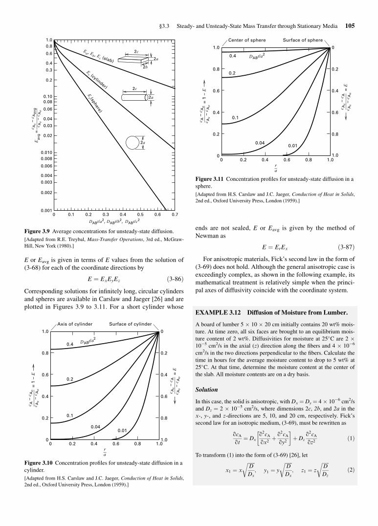
C03 09/29/2010 Page 105
E or Eavg is given in terms of E values from the solution of
(3-68) for each of the coordinate directions by
E ¼ ExEyEz ð3-86ÞCorresponding solutions for infinitely long, circular cylinders
and spheres are available in Carslaw and Jaeger [26] and are
plotted in Figures 3.9 to 3.11. For a short cylinder whose
ends are not sealed, E or Eavg is given by the method of
Newman as
E ¼ ErEx ð3-87ÞFor anisotropic materials, Fick’s second law in the form of
(3-69) does not hold. Although the general anisotropic case is
exceedingly complex, as shown in the following example, its
mathematical treatment is relatively simple when the princi-
pal axes of diffusivity coincide with the coordinate system.
EXAMPLE 3.12 Diffusion of Moisture from Lumber.
A board of lumber 5 � 10 � 20 cm initially contains 20 wt% mois-
ture. At time zero, all six faces are brought to an equilibrium mois-
ture content of 2 wt%. Diffusivities for moisture at 25�C are 2 �10�5 cm2/s in the axial (z) direction along the fibers and 4 � 10�6
cm2/s in the two directions perpendicular to the fibers. Calculate the
time in hours for the average moisture content to drop to 5 wt% at
25�C. At that time, determine the moisture content at the center of
the slab. All moisture contents are on a dry basis.
Solution
In this case, the solid is anisotropic, with Dx¼ Dy ¼ 4 � 10�6 cm2/s
and Dz ¼ 2 � 10�5 cm2/s, where dimensions 2c, 2b, and 2a in the
x-, y-, and z-directions are 5, 10, and 20 cm, respectively. Fick’s
second law for an isotropic medium, (3-69), must be rewritten as
qcAqt¼ Dx
q2cAqx2þ q2cA
qy2
� �þ Dz
q2cAqz2
ð1Þ
To transform (1) into the form of (3-69) [26], let
x1 ¼ x
ffiffiffiffiffiffiD
Dx
r; y1 ¼ y
ffiffiffiffiffiffiD
Dx
r; z1 ¼ z
ffiffiffiffiffiffiD
Dz
rð2Þ
Ea , E
b , Ec (slab)
Er (cylinder)
Es (sphere)
DABt/a2, DABt/b2, DABt/c2
0 0.1 0.2 0.3 0.4 0.5 0.6 0.7
1.00.8
0.6
0.4
0.3
0.2
0.100.08
0.06
0.04
0.03
0.02
0.0100.008
0.006
0.004
0.003
0.002
0.001
2c
2a
2a
2c
2a
2b
Eav
g =
c As –
cA
avg
c As –
cA
o
Figure 3.9 Average concentrations for unsteady-state diffusion.
[Adapted from R.E. Treybal, Mass-Transfer Operations, 3rd ed., McGraw-
Hill, New York (1980).]
ra
DABt/a2
0 0.2 0.4 0.6 0.8 1.0
= 1
– E
c A –
cA
oc A
s – c
Ao
0.4
0.2
0.1
0.040.01
0
0.2
0.4
0.6
0.8
1.0
1.0
0.8
0.6
0.4
0.2
0
Axis of cylinder
c As –
cA
c As –
cA
o=
E
Surface of cylinder
Figure 3.10 Concentration profiles for unsteady-state diffusion in a
cylinder.
[Adapted from H.S. Carslaw and J.C. Jaeger, Conduction of Heat in Solids,
2nd ed., Oxford University Press, London (1959).]
ra
DABt/a2
0 0.2 0.4 0.6 0.8 1.0
= 1
– E
c A –
cA
oc A
s – c
Ao
0.4
0.2
0.1
0.040.01
0
0.2
0.4
0.6
0.8
1.0
1.0
0.8
0.6
0.4
0.2
0
Center of sphere
c As –
cA
c As –
cA
o=
E
Surface of sphere
Figure 3.11 Concentration profiles for unsteady-state diffusion in a
sphere.
[Adapted from H.S. Carslaw and J.C. Jaeger, Conduction of Heat in Solids,
2nd ed., Oxford University Press, London (1959).]
§3.3 Steady- and Unsteady-State Mass Transfer through Stationary Media 105
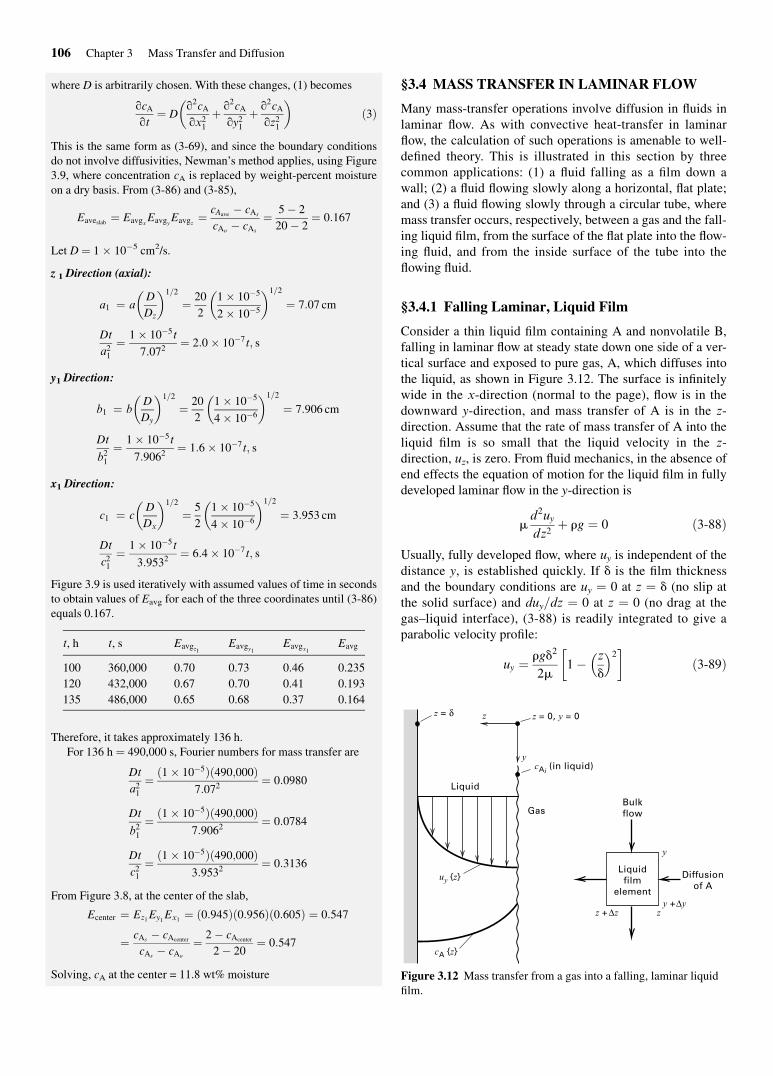
C03 09/29/2010 Page 106
where D is arbitrarily chosen. With these changes, (1) becomes
qcAqt¼ D
q2cAqx21þ q2cA
qy21þ q2cA
qz21
� �ð3Þ
This is the same form as (3-69), and since the boundary conditions
do not involve diffusivities, Newman’s method applies, using Figure
3.9, where concentration cA is replaced by weight-percent moisture
on a dry basis. From (3-86) and (3-85),
Eaveslab ¼ EavgxEavgyEavgz ¼cAave� cAs
cAo� cAs
¼ 5� 2
20� 2¼ 0:167
Let D ¼ 1 � 10�5 cm2/s.
z 1 Direction (axial):
a1 ¼ aD
Dz
� �1=2
¼ 20
2
1� 10�5
2� 10�5
� �1=2
¼ 7:07 cm
Dt
a21¼ 1� 10�5t
7:072¼ 2:0� 10�7t; s
y1 Direction:
b1 ¼ bD
Dy
� �1=2
¼ 20
2
1� 10�5
4� 10�6
� �1=2
¼ 7:906 cm
Dt
b21¼ 1� 10�5t
7:9062¼ 1:6� 10�7t; s
x1 Direction:
c1 ¼ cD
Dx
� �1=2
¼ 5
2
1� 10�5
4� 10�6
� �1=2
¼ 3:953 cm
Dt
c21¼ 1� 10�5t
3:9532¼ 6:4� 10�7t; s
Figure 3.9 is used iteratively with assumed values of time in seconds
to obtain values of Eavg for each of the three coordinates until (3-86)
equals 0.167.
t, h t, s Eavgz1Eavgy1
Eavgx1Eavg
100 360,000 0.70 0.73 0.46 0.235
120 432,000 0.67 0.70 0.41 0.193
135 486,000 0.65 0.68 0.37 0.164
Therefore, it takes approximately 136 h.
For 136 h ¼ 490,000 s, Fourier numbers for mass transfer are
Dt
a21¼ ð1� 10�5Þð490;000Þ
7:072¼ 0:0980
Dt
b21¼ ð1� 10�5Þð490;000Þ
7:9062¼ 0:0784
Dt
c21¼ ð1� 10�5Þð490;000Þ
3:9532¼ 0:3136
From Figure 3.8, at the center of the slab,
Ecenter ¼ Ez1Ey1Ex1 ¼ ð0:945Þð0:956Þð0:605Þ ¼ 0:547
¼ cAs� cAcenter
cAs� cAo
¼ 2� cAcenter
2� 20¼ 0:547
Solving, cA at the center = 11.8 wt% moisture
§3.4 MASS TRANSFER IN LAMINAR FLOW
Many mass-transfer operations involve diffusion in fluids in
laminar flow. As with convective heat-transfer in laminar
flow, the calculation of such operations is amenable to well-
defined theory. This is illustrated in this section by three
common applications: (1) a fluid falling as a film down a
wall; (2) a fluid flowing slowly along a horizontal, flat plate;
and (3) a fluid flowing slowly through a circular tube, where
mass transfer occurs, respectively, between a gas and the fall-
ing liquid film, from the surface of the flat plate into the flow-
ing fluid, and from the inside surface of the tube into the
flowing fluid.
§3.4.1 Falling Laminar, Liquid Film
Consider a thin liquid film containing A and nonvolatile B,
falling in laminar flow at steady state down one side of a ver-
tical surface and exposed to pure gas, A, which diffuses into
the liquid, as shown in Figure 3.12. The surface is infinitely
wide in the x-direction (normal to the page), flow is in the
downward y-direction, and mass transfer of A is in the z-
direction. Assume that the rate of mass transfer of A into the
liquid film is so small that the liquid velocity in the z-
direction, uz, is zero. From fluid mechanics, in the absence of
end effects the equation of motion for the liquid film in fully
developed laminar flow in the y-direction is
md2uy
dz2þ rg ¼ 0 ð3-88Þ
Usually, fully developed flow, where uy is independent of the
distance y, is established quickly. If d is the film thickness
and the boundary conditions are uy ¼ 0 at z ¼ d (no slip at
the solid surface) and duy=dz ¼ 0 at z ¼ 0 (no drag at the
gas–liquid interface), (3-88) is readily integrated to give a
parabolic velocity profile:
uy ¼ rgd2
2m1� z
d
� 2� �ð3-89Þ
Liquidfilm
element
BulkflowGas
Diffusionof A
Liquid
z = δ z
z +Δzy +Δy
z = 0, y = 0
y
y
z
uy {z}
cAi (in liquid)
cA {z}
Figure 3.12 Mass transfer from a gas into a falling, laminar liquid
film.
106 Chapter 3 Mass Transfer and Diffusion

C03 09/29/2010 Page 107
The maximum liquid velocity occurs at z ¼ 0,
ðuyÞmax ¼rgd2
2mð3-90Þ
The bulk-average velocity in the liquid film is
�uy ¼R d0uydz
d¼ rgd2
3mð3-91Þ
Thus, with no entrance effects, the film thickness for fully
developed flow is independent of location y and is
d ¼ 3�uym
rg
� �1=2
¼ 3mG
r2g
� �1=3
ð3-92Þ
where G ¼ liquid film flow rate per unit width of film, W. For
film flow, the Reynolds number, which is the ratio of the iner-
tial force to the viscous force, is
NRe ¼ 4rH�uyr
m¼ 4d�uyr
m¼ 4G
mð3-93Þ
where rH ¼ hydraulic radius ¼ (flow cross section)=(wettedperimeter) ¼ (Wd)=W ¼ d and, by continuity, G ¼ �uyrd.
Grimley [32] found that for NRe < 8 to 25, depending on
surface tension and viscosity, flow in the film is laminar and
the interface between the liquid film and gas is flat. The value
of 25 is obtained with water. For 8 to 25 < NRe < 1,200, the
flow is still laminar, but ripples may appear at the interface
unless suppressed by the addition of wetting agents.
For a flat interface and a low rate of mass transfer of A,
Eqs. (3-88) to (3-93) hold, and the film velocity profile is
given by (3-89). Consider a mole balance on A for an incre-
mental volume of liquid film of constant density, as shown in
Figure 3.12. Neglect bulk flow in the z-direction and axial
diffusion in the y-direction. Thus, mass transfer of A from
the gas into the liquid occurs only by molecular diffusion in
the z-direction. Then, at steady state, neglecting accumula-
tion or depletion of A in the incremental volume (quasi-
steady-state assumption),
�DABðDyÞðDxÞ qcAqz
� �
z
þ uycAjyðDzÞðDxÞ
¼ �DABðDyÞðDxÞ qcAqz
� �
zþDzþ uycAjyþDyðDzÞðDxÞ
ð3-94ÞRearranging and simplifying (3-94),
uycAjyþDy � uycAjyDy
� �¼ DAB
ðqcA=qzÞzþDz � ðqcA=qzÞzDz
� �
ð3-95Þwhich, in the limit, as Dz! 0 and Dy! 0, becomes
uyqcAqy¼ DAB
q2cAqz2
ð3-96Þ
Substituting the velocity profile of (3-89) into (3-96),
rgd2
2m1� z
d
� 2� �qcAqy¼ DAB
q2cAqz2
ð3-97Þ
This PDE was solved by Johnstone and Pigford [33] and
Olbrich and Wild [34] for the following boundary conditions,
where the initial concentration of A in the liquid film is cAo:
cA ¼ cAiat z ¼ 0 for y > 0
cA ¼ cAoat y ¼ 0 for 0 < z < d
qcA=qz ¼ 0 at z ¼ d for 0 < y < L
where L ¼ height of the vertical surface. The solution of
Olbrich and Wild is in the form of an infinite series, giving
cA as a function of z and y. Of greater interest, however, is
the average concentration of A in the film at the bottom of
the wall, where y ¼ L, which, by integration, is
�cAy¼ 1
�uyd
Z d
0
uycAydz ð3-98Þ
For the condition y ¼ L, the result is
cAi� �cAL
cAi� cAo
¼ 0:7857e�5:1213h þ 0:09726e�39:661h
þ 0:036093e�106:25h þ � � �ð3-99Þ
where
h ¼ 2DABL
3d2�uy¼ 8=3
NReNScðd=LÞ ¼8=3
ðd=LÞNPeM
ð3-100Þ
NSc ¼ Schmidt number ¼ m
rDAB
¼ momentum diffusivity;m=r
mass diffusivity;DAB
ð3-101Þ
NPeM ¼ NReNSc ¼ Peclet number for mass transfer
¼ 4d�uyDAB
ð3-102Þ
The Schmidt number is analogous to the Prandtl number,
used in heat transfer:
NPr ¼ CPm
k¼ ðm=rÞðk=rCPÞ ¼
momentum diffusivity
thermal diffusivity
The Peclet number for mass transfer is analogous to the
Peclet number for heat transfer:
NPeH ¼ NReNPr ¼ 4d�uyCPr
k
Both are ratios of convective to molecular transport.
The total rate of absorption of A from the gas into the liq-
uid film for height L and widthW is
nA ¼ �uydWð�cAL� cAo
Þ ð3-103Þ
§3.4.2 Mass-Transfer Coefficients
Mass-transfer problems involving flowing fluids are often
solved using mass-transfer coefficients, which are analogous
to heat-transfer coefficients. For the latter, Newton’s law of
§3.4 Mass Transfer in Laminar Flow 107

C03 09/29/2010 Page 108
cooling defines a heat-transfer coefficient, h:
Q ¼ hADT ð3-104ÞwhereQ¼ rate of heat transfer, A¼ area for heat transfer (nor-
mal to the direction of heat transfer), and DT ¼ temperature-
driving force.
For mass transfer, a composition-driving force replaces
DT. Because composition can be expressed in a number of
ways, different mass-transfer coefficients result. If concentra-
tion is used, DcA is selected as the driving force and
nA ¼ kcADcA ð3-105Þ
which defines a mass-transfer coefficient, kc, in mol/time-
area-driving force, for a concentration driving force.
Unfortunately, no name is in general use for (3-105).
For the falling laminar film, DcA ¼ cAi� �cA, where �cA is
the bulk average concentration of A in the film, which varies
with vertical location, y, because even though cAiis indepen-
dent of y, the average film concentration of A increases with
y. A theoretical expression for kc in terms of diffusivity is
formed by equating (3-105) to Fick’s first law at the gas–
liquid interface:
kcAðcAj� �cAÞ ¼ �DABA
qcAqz
� �
z¼0ð3-106Þ
Although this is the most widely used approach for defin-
ing a mass-transfer coefficient, for a falling film it fails
because ðqcA=qzÞ at z ¼ 0 is not defined. Therefore, another
approach is used. For an incremental height,
nA ¼ �uydW d�cA ¼ kcðcA? � �cAÞW dy ð3-107ÞThis defines a local value of kc, which varies with distance
y because �cA varies with y. An average value of kc, over
height L, can be defined by separating variables and integrat-
ing (3-107):
kcavg ¼R L0kcdy
L¼
�uydR cALcAo½d�cA=ðcAi
� �cA�L
¼ �uyd
LlncAi� cAo
cAi� �cAL
ð3-108Þ
The argument of the natural logarithm in (3-108) is ob-
tained from the reciprocal of (3-99). For values of h in (3-
100) greater than 0.1, only the first term in (3-99) is signifi-
cant (error is less than 0.5%). In that case,
kcavg ¼�uyd
Llne5:1213h
0:7857ð3-109Þ
Since ln ex ¼ x,
kcavg ¼�uyd
Lð0:241þ 5:1213hÞ ð3-110Þ
In the limit for large h, using (3-100) and (3-102), (3-110)
becomes
kcavg ¼ 3:414DAB
dð3-111Þ
As suggested by the Nusselt number, NNu¼ hd=k for
heat transfer, where d is a characteristic length, a Sherwood
number for mass transfer is defined for a falling film as
NShavg ¼kcavgd
DAB
ð3-112Þ
From (3-111), NShavg ¼ 3:414, which is the smallest value the
Sherwood number can have for a falling liquid film. The
average mass-transfer flux of A is
NAavg¼ nAavg
A¼ kcavgðcAi
� �cAÞmean ð3-113Þ
For h < 0.001 in (3-100), when the liquid-film flow
regime is still laminar without ripples, the time of contact of
gas with liquid is short and mass transfer is confined to the
vicinity of the interface. Thus, the film acts as if it were infi-
nite in thickness. In this limiting case, the downward velocity
of the liquid film in the region of mass transfer is uymax, and
(3-96) becomes
uymax
qcAqy¼ DAB
q2cAqz2
ð3-114Þ
Since from (3-90) and (3-91) uymax¼ 3uy=2, (3-114) becomes
qcAqy¼ 2DAB
3�uy
� �q2cAqz2
ð3-115Þ
where the boundary conditions are
cA ¼ cAofor z > 0 and y > 0
cA ¼ cAifor z ¼ 0 and y > 0
cA ¼ cAifor large z and y > 0
Equation (3-115) and the boundary conditions are equivalent
to the case of the semi-infinite medium in Figure 3.6. By
analogy to (3-68), (3-75), and (3-76), the solution is
E ¼ 1� u ¼ cAi� cA
cAi� cAo
¼ erfz
2ffiffiffiffiffiffiffiffiffiffiffiffiffiffiffiffiffiffiffiffiffiffi2DABy=3�uy
p !
ð3-116Þ
Assuming that the driving force for mass transfer in the film
is cAi� cA0
, Fick’s first law can be used at the gas–liquid
interface to define a mass-transfer coefficient:
NA ¼ �DAB
qcAqz
����z¼0¼ kcðcAi
� cAoÞ ð3-117Þ
To obtain the gradient of cA at z ¼ 0 from (3-116), note that
the error function is defined as
erf z ¼ 2ffiffiffiffipp
Z z
0
e�t2
dt ð3-118Þ
Combining (3-118) with (3-116) and applying the Leibnitz
differentiation rule,
qcAqz
����z¼0¼ �ðcAi
� cAoÞffiffiffiffiffiffiffiffiffiffiffiffiffiffiffiffiffi3�uy
2pDABy
sð3-119Þ
Substituting (3-119) into (3-117) and introducing the Peclet
number for mass transfer from (3-102), the local mass-
108 Chapter 3 Mass Transfer and Diffusion

C03 09/29/2010 Page 109
transfer coefficient as a function of distance down from the
top of the wall is obtained:
kc ¼ffiffiffiffiffiffiffiffiffiffiffiffiffiffiffiffiffiffiffiffiffi3D2
ABNPeM
8pyd
s
¼ffiffiffiffiffiffiffiffiffiffiffiffiffiffi3DABG
2pydr
sð3-120Þ
The average value of kc over the film height, L, is obtained by
integrating (3-120) with respect to y, giving
kcavg ¼ffiffiffiffiffiffiffiffiffiffiffiffiffiffi6DABG
pdrL
s¼
ffiffiffiffiffiffiffiffiffiffiffiffiffiffiffiffiffiffiffiffiffi3D2
AB
2pdLNPeM
s
ð3-121Þ
Combining (3-121) with (3-112) and (3-102),
NShavg ¼ffiffiffiffiffiffiffiffiffiffiffiffiffiffiffiffiffiffiffi3d
2pLNPeM
r¼
ffiffiffiffiffiffiffi4
ph
sð3-122Þ
where, by (3-108), the proper mean concentration driving
force to use with kcavg is the log mean. Thus,
ðcAi� �cAÞmean ¼ ðcAi
� �cAÞLM¼ ðcAi
� cAoÞ � ðcAi
� cALÞ
ln½ðcAi� cAo
Þ=ðcAi� �cAL
Þ�ð3-123Þ
When ripples are present, values of kcavg and NShavg are con-
siderably larger than predicted by the above equations.
The above development shows that asymptotic, closed-
form solutions are obtained with relative ease for large and
small values of h, as defined by (3-100). These limits, in
terms of the average Sherwood number, are shown in Figure
3.13. The general solution for intermediate values of h is not
available in closed form. Similar limiting solutions for large
and small values of dimensionless groups have been obtained
for a large variety of transport and kinetic phenomena
(Churchill [35]). Often, the two limiting cases can be patched
together to provide an estimate of the intermediate solution,
if an intermediate value is available from experiment or the
general numerical solution. The procedure is discussed by
Churchill and Usagi [36]. The general solution of Emmert
and Pigford [37] to the falling, laminar liquid film problem is
included in Figure 3.13.
EXAMPLE 3.13 Absorption of CO2 into a Falling
Water Film.
Water (B) at 25�C, in contact with CO2 (A) at 1 atm, flows as a film
down a wall 1 m wide and 3 m high at a Reynolds number of 25.
Estimate the rate of absorption of CO2 into water in kmol/s:
DAB ¼ 1:96� 10�5cm2/s; r ¼ 1:0 g/cm3;mL ¼ 0:89 cP ¼ 0:00089 kg/m-s
Solubility of CO2 at 1 atm and 25�C ¼ 3.4 � 10�5 mol/cm3.
Solution
From (3-93), G ¼ NRem
4¼ 25ð0:89Þð0:001Þ
4¼ 0:00556
kg
m-s
From (3-101),
NSc ¼ m
rDAB
¼ ð0:89Þð0:001Þð1:0Þð1;000Þð1:96� 10�5Þð10�4Þ ¼ 454
From (3-92),
d ¼ 3ð0:89Þð0:001Þð0:00556Þ1:02ð1:000Þ2ð9:807Þ
" #1=3¼ 1:15� 10�4 m
From (3-90) and (3-91), �uy ¼ ð2=3Þuymax. Therefore,
�uy ¼ 2
3
ð1:0Þð1;000Þð9:807Þð1:15� 10�4Þ22ð0:89Þð0:001Þ
" #¼ 0:0486m/s
From (3-100),
h ¼ 8=3
ð25Þð454Þ½ð1:15� 10�4Þ=3� ¼ 6:13
Therefore, (3-111) applies, giving
kcavg ¼3:41ð1:96� 10�5Þð10�4Þ
1:15� 10�4¼ 5:81� 10�5 m/s
General solution
Short residence-time solution
Eq. (3-122)
Long residence-time solutionEq. (3-111)
100
10
10.001
Sh
erw
oo
d n
um
ber
8/3( /L)NPeM
=ηδ
0.10.01 1 10
Figure 3.13 Limiting and general solutions for mass transfer to a falling, laminar liquid film.
§3.4 Mass Transfer in Laminar Flow 109

C03 09/29/2010 Page 110
To obtain the rate of absorption, �cALis determined. From (3-103)
and (3-113),
nA ¼ �uydWð�cAL� cAo
Þ ¼ kcavgAð�cAL� cAo
Þln½ðcAi
� cAoÞ=ðcAi
� cAL�
Thus, lncAi� cAo
cAi� �cAL
� �¼ kcavgA
�uydW
Solving for �cAL,
�cAL¼ cAi
� ðcAi� cAo
Þ exp � kcavgA
�uydW
� �
L ¼ 3m; W ¼ 1m; A ¼ WL ¼ ð1Þð3Þ ¼ 3m2
cAo¼ 0; cAi
¼ 3:4� 10�5mol/cm3 ¼ 3:4� 10�2 kmol/m3
�cAL¼ 3:4� 10�2 1� exp � ð5:81� 10�5Þð3Þ
ð0:0486Þð1:15� 10�4Þð1Þ� ��
¼ 3:4� 10�2 kmol/m3
Thus, the exiting liquid film is saturated with CO2, which implies
equilibrium at the gas–liquid interface. From (3-103),
nA ¼ 0:0486ð1:15� 10�4Þð3:4� 10�2Þ ¼ 1:9� 10�7 kmol/s
§3.4.3 Molecular Diffusion to a Fluid FlowingAcross a Flat Plate—The Boundary Layer Concept
Consider the flow of fluid (B) over a thin, horizontal, flat
plate, as shown in Figure 3.14. Some possibilities for mass
transfer of species A into B are: (1) the plate consists of ma-
terial A, which is slightly soluble in B; (2) A is in the pores of
an inert solid plate from which it evaporates or dissolves into
B; and (3) the plate is a dense polymeric membrane through
which A can diffuse and pass into fluid B. Let the fluid veloc-
ity profile upstream of the plate be uniform at a free-system
velocity of uo. As the fluid passes over the plate, the velocity
ux in the direction x of flow is reduced to zero at the wall,
which establishes a velocity profile due to drag. At a certain
distance z that is normal to and upward out from the plate
surface, the fluid velocity is 99% of uo. This distance, which
increases with increasing distance x from the leading edge of
the plate, is defined as the velocity boundary-layer thickness,
d. Essentially all flow retardation is assumed to occur in the
boundary layer, as first suggested by Prandtl [38]. The
buildup of this layer, the velocity profile, and the drag force
can be determined for laminar flow by solving the Navier–
Stokes equations.
For a Newtonian fluid of constant density and viscosity,
with no pressure gradients in the x- or y-directions, these
equations for the boundary layer are
quxqxþ quz
qz¼ 0 ð3-124Þ
uxquxqxþ uz
quxqz¼ m
r
q2uxqz2
� �ð3-125Þ
The boundary conditions are
ux ¼ uo at x ¼ 0 for z > 0; ux ¼ 0 at z ¼ 0 for x > 0
ux ¼ uo at z ¼ 1 for x > 0; uz ¼ 0 at z ¼ 0 for x > 0
A solution of (3-124) and (3-125) was first obtained by Bla-
sius [39], as described by Schlichting [40]. The result in
terms of a local friction factor, fx; a local shear stress at the
wall, twx; and a local drag coefficient at the wall, CDx
, is
CDx
2¼ f x
2¼ twx
ru2o¼ 0:322
N0:5Rex
ð3-126Þ
where NRex ¼xuor
mð3-127Þ
The drag is greatest at the leading edge of the plate, where
the Reynolds number is smallest. Values of the drag co-
efficient obtained by integrating (3-126) from x ¼ 0 to L are
CDavg
2¼ f avg
2¼ 0:664
ðNReLÞ0:5ð3-128Þ
The thickness of the velocity boundary layer increases with
distance along the plate:
d
x¼ 4:96
N0:5Rex
ð3-129Þ
A reasonably accurate expression for a velocity profile was
obtained by Pohlhausen [41], who assumed the empirical form
of the velocity in the boundary layer to be ux¼ C1zþ C2z3.
If the boundary conditions
ux ¼ 0 at z ¼ 0; ux ¼ uo at z ¼ d; qux=qz ¼ 0 at z ¼ d
are applied to evaluate C1 and C2, the result is
ux
uo¼ 1:5
z
d
� � 0:5
z
d
� 3ð3-130Þ
This solution is valid only for a laminar boundary layer,
which by experiment persists up to NRex ¼ 5� 105.
When mass transfer of A from the surface of the plate into
the boundary layer occurs, a species continuity equation
applies:
uxqcAqxþ uz
qcAqz¼ DAB
q2cAqx2
� �ð3-131Þ
If mass transfer begins at the leading edge of the plate and
the concentration in the fluid at the solid–fluid interface is
Velocityboundary
layer
Freestream
Flat plate
uxux
uo
uo
x
zux
uo
uo
xδ
Figure 3.14 Laminar boundary layer for flow across a flat plate.
110 Chapter 3 Mass Transfer and Diffusion
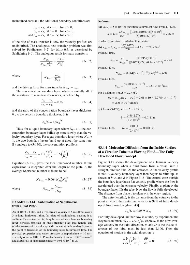
C03 09/29/2010 Page 111
maintained constant, the additional boundary conditions are
cA ¼ cAoat x ¼ 0 for z > 0;
cA ¼ cAiat z ¼ 0 for x > 0;
and cA ¼ cAoat z ¼ 1 for x > 0
If the rate of mass transfer is low, the velocity profiles are
undisturbed. The analogous heat-transfer problem was first
solved by Pohlhausen [42] for NPr> 0.5, as described by
Schlichting [40]. The analogous result for mass transfer is
NShx
NRexN1=3Sc
¼ 0:332
N0:5Rex
ð3-132Þ
whereNShx ¼
xkcxDAB
ð3-133Þ
and the driving force for mass transfer is cAi� cAo
.
The concentration boundary layer, where essentially all of
the resistance to mass transfer resides, is defined by
cAi� cA
cAi� cAo
¼ 0:99 ð3-134Þ
and the ratio of the concentration boundary-layer thickness,
dc, to the velocity boundary thickness, d, is
dc=d ¼ 1=N1=3Sc ð3-135Þ
Thus, for a liquid boundary layer where NSc> 1, the con-
centration boundary layer builds up more slowly than the ve-
locity boundary layer. For a gas boundary layer where NSc �1, the two boundary layers build up at about the same rate.
By analogy to (3-130), the concentration profile is
cAi� cA
cAi� cAo
¼ 1:5z
dc
� �� 0:5
z
dc
� �3
ð3-136Þ
Equation (3-132) gives the local Sherwood number. If this
expression is integrated over the length of the plate, L, the
average Sherwood number is found to be
NShavg ¼ 0:664 N1=2ReL
N1=3Sc ð3-137Þ
where NShavg ¼Lkcavg
DAB
ð3-138Þ
EXAMPLE 3.14 Sublimation of Naphthalenefrom a Flat Plate.
Air at 100�C, 1 atm, and a free-stream velocity of 5 m/s flows over a
3-m-long, horizontal, thin, flat plate of naphthalene, causing it to
sublime. Determine the: (a) length over which a laminar boundary
layer persists, (b) rate of mass transfer over that length, and
(c) thicknesses of the velocity and concentration boundary layers at
the point of transition of the boundary layer to turbulent flow. The
physical properties are: vapor pressure of naphthalene ¼ 10 torr;
viscosity of air ¼ 0.0215 cP; molar density of air ¼ 0.0327 kmol/m3;
and diffusivity of naphthalene in air¼ 0.94� 10�5 m2/s.
Solution
(a) NRex ¼ 5� 105 for transition to turbulent flow. From (3-127),
x ¼ L ¼ mNRex
uor¼ ½ð0:0215Þð0:001Þ�ð5� 105Þ
ð5Þ½ð0:0327Þð29Þ� ¼ 2:27 m
at which transition to turbulent flow begins.
(b) cAo¼ 0; cAi
¼ 10ð0:0327Þ760
¼ 4:3� 10�4 kmol/m3.
From (3-101),
NSc ¼ m
rDAB
¼ ½ð0:0215Þð0:001Þ�½ð0:0327Þð29Þ�ð0:94� 10�5Þ ¼ 2:41
From (3-137),
NShavg ¼ 0:664ð5� 105Þ1=2ð2:41Þ1=3 ¼ 630
From (3-138),
kcavg ¼630ð0:94� 10�5Þ
2:27¼ 2:61� 10�3m/s
For a width of 1 m, A ¼ 2.27 m2,
nA ¼ kcavgAðcAi� cAo
Þ ¼ 2:61� 10�3ð2:27Þð4:3� 10�4Þ¼ 2:55� 10�6kmol/s
(c) From (3-129), at x ¼ L ¼ 2.27 m,
d ¼ 3:46ð2:27Þð5� 105Þ0:5 ¼ 0:0111 m
From (3-135), dc ¼ 0:0111
ð2:41Þ1=3¼ 0:0083 m
§3.4.4 Molecular Diffusion from the Inside Surfaceof a Circular Tube to a Flowing Fluid—The FullyDeveloped Flow Concept
Figure 3.15 shows the development of a laminar velocity
boundary layer when a fluid flows from a vessel into a
straight, circular tube. At the entrance, a, the velocity profile
is flat. A velocity boundary layer then begins to build up, as
shown at b, c, and d in Figure 3.15. The central core outside
the boundary layer has a flat velocity profile where the flow is
accelerated over the entrance velocity. Finally, at plane e, the
boundary layer fills the tube. Now the flow is fully developed.
The distance from plane a to plane e is the entry region.
The entry length Le is the distance from the entrance to the
point at which the centerline velocity is 99% of fully devel-
oped flow. From Langhaar [43],
Le=D ¼ 0:0575 NRe ð3-139ÞFor fully developed laminar flow in a tube, by experiment the
Reynolds number, NRe ¼ D�uxr=m, where �ux is the flow-aver-age velocity in the axial direction, x, and D is the inside di-
ameter of the tube, must be less than 2,100. Then the
equation of motion in the axial direction is
m
r
qqr
rquxqr
� �� dP
qx¼ 0 ð3-140Þ
§3.4 Mass Transfer in Laminar Flow 111

C03 09/29/2010 Page 112
with boundary conditions:
r ¼ 0 ðaxis of the tubeÞ; qux=qr ¼ 0
and r ¼ rwðtube wallÞ; ux ¼ 0
Equation (3-140) was integrated by Hagen in 1839 and Pois-
euille in 1841. The resulting equation for the velocity profile,
in terms of the flow-average velocity, is
ux ¼ 2�ux 1� r
rw
� �2" #
ð3-141Þ
or, in terms of the maximum velocity at the tube axis,
ux ¼ uxmax1� r
rw
� �2" #
ð3-142Þ
According to (3-142), the velocity profile is parabolic.
The shear stress, pressure drop, and Fanning friction fac-
tor are obtained from solutions to (3-140):
tw ¼ �m quxqr
� �����r¼rw¼ 4m�ux
rwð3-143Þ
� dP
dx¼ 32m�ux
D2¼ 2fr�u2x
Dð3-144Þ
with f ¼ 16
NRe
ð3-145Þ
At the upper limit of laminar flow, NRe ¼ 2,100, and Le=D ¼121, but at NRe ¼ 100, Le=D is only 5.75. In the entry region,
the friction factor is considerably higher than the fully devel-
oped flow value given by (3-145). At x ¼ 0, f is infinity, but it
decreases exponentially with x, approaching the fully devel-
oped flow value at Le. For example, for NRe ¼ 1,000, (3-145)
gives f ¼ 0.016, with Le=D ¼ 57.5. From x ¼ 0 to x=D ¼5.35, the average friction factor from Langhaar is 0.0487,
which is three times the fully developed value.
In 1885, Graetz [44] obtained a solution to the problem of
convective heat transfer between the wall of a circular tube,
at a constant temperature, and a fluid flowing through the
tube in fully developed laminar flow. Assuming constant
properties and negligible conduction in the axial direction,
the energy equation, after substituting (3-141) for ux, is
2�ux 1� r
rw
� �2" #
qTqx¼ k
rCp
1
r
qqr
rqTqr
� �� �ð3-146Þ
with boundary conditions:
x ¼ 0 ðwhere heat transfer beginsÞ; T ¼ T0; for all r
x > 0; r ¼ rw; T ¼ Ti and x > 0; r ¼ 0; qT=qr ¼ 0
The analogous species continuity equation for mass trans-
fer, neglecting bulk flow in the radial direction and axial dif-
fusion, is
2�ux 1� r
rw
� �2" #
qcAqx¼ DAB
1
r
qqr
rqcAqr
� �� �ð3-147Þ
with analogous boundary conditions.
The Graetz solution of (3-147) for the temperature or con-
centration profile is an infinite series that can be obtained
from (3-146) by separation of variables using the method of
Frobenius. A detailed solution is given by Sellars, Tribus, and
Klein [45]. The concentration profile yields expressions for
the mass-transfer coefficient and the Sherwood number. For
large x, the concentration profile is fully developed and the
local Sherwood number, NShx , approaches a limiting value of
3.656. When x is small, such that the concentration boundary
layer is very thin and confined to a region where the fully
developed velocity profile is linear, the local Sherwood num-
ber is obtained from the classic Leveque [46] solution, pre-
sented by Knudsen and Katz [47]:
NShx ¼kcxD
DAB
¼ 1:077NPeM
ðx=DÞ� �1=3
ð3-148Þ
where NPeM ¼D�uxDAB
ð3-149Þ
The limiting solutions, together with the general Graetz so-
lution, are shown in Figure 3.16, where NShx ¼ 3:656 is valid
for NPeM=ðx=DÞ < 4 and (3-148) is valid for NPeM=ðx=DÞ >100. These solutions can be patched together if a point from
the general solution is available at the intersection in a manner
like that discussed in §3.4.2.
Where mass transfer occurs, an average Sherwood number
is derived by integrating the general expression for the local
En
tran
ceve
loci
ty =
ux
Entrance
Thickness ofboundary layer
Edge ofboundary layer
Fully developedtube flow
a b
x
c d e
Figure 3.15 Buildup of a laminar velocity boundary layer for flow in a circular tube.
112 Chapter 3 Mass Transfer and Diffusion

C03 09/29/2010 Page 113
Sherwood number. An empirical representation for that aver-
age, proposed by Hausen [48], is
NShavg ¼ 3:66þ 0:0668½NPeM=ðx=DÞ�1þ 0:04½NPeM=ðx=DÞ�2=3
ð3-150Þ
which is based on a log-mean concentration driving force.
EXAMPLE 3.15 Mass Transfer of Benzoic Acid into
Water Flowing in Laminar Motion Through a Tube.
Linton and Sherwood [49] dissolved tubes of benzoic acid (A) into
water (B) flowing in laminar flow through the tubes. Their data
agreed with predictions based on the Graetz and Leveque equations.
Consider a 5.23-cm-inside-diameter, 32-cm-long tube of benzoic
acid, preceded by 400 cm of straight metal pipe wherein a fully
developed velocity profile is established. Water enters at 25�C at a
velocity corresponding to a Reynolds number of 100. Based on
property data at 25�C, estimate the average concentration of benzoic
acid leaving the tube before a significant increase in the inside diam-
eter of the benzoic acid tube occurs because of dissolution. The
properties are: solubility of benzoic acid in water ¼ 0.0034 g/cm3;
viscosity of water ¼ 0.89 cP ¼ 0.0089 g/cm-s; and diffusivity of
benzoic acid in water at infinite dilution ¼ 9.18 � 10�6 cm2/s.
Solution
NSc ¼ 0:0089
ð1:0Þð9:18� 10�6Þ ¼ 970
NRe ¼ D�uxr
m¼ 100
from which �ux ¼ ð100Þð0:0089Þð5:23Þð1:0Þ ¼ 0:170 cm/s
From (3-149), NPeM ¼ð5:23Þð0:170Þ9:18� 10�6
¼ 9:69� 104
x
D¼ 32
5:23¼ 6:12
NPeM
ðx=DÞ ¼9:69� 104
6:12¼ 1:58� 104
From (3-150),
NShavg ¼ 3:66þ 0:0668ð1:58� 104Þ1þ 0:04ð1:58� 104Þ2=3
¼ 44
kcavg ¼ NShavg
DAB
D
� �¼ 44
ð9:18� 10�6Þ5:23
¼ 7:7� 10�5cm/s
Using a log mean driving force,
nA ¼ �uxSð�cAx� cAo
Þ ¼ kcavgA½ðcAi
� cAoÞ � ðcAi
� �cAx�
ln½ðcAi� cAo
Þ=ðcAi� �cAx
Þ�where S is the cross-sectional area for flow. Simplifying,
lncAi� cAo
cAi� �cAx
� �¼ kcavgA
�uxS
cAo¼ 0 and cAi
¼ 0:0034 g/cm3
S ¼ pD2
4¼ ð3:14Þð5:23Þ
2
4¼ 21:5 cm2 and
A ¼ pDx ¼ ð3:14Þð5:23Þð32Þ ¼ 526 cm2
ln0:0034
0:0034� �cAx
� �¼ ð7:7� 10�5Þð526Þ
ð0:170Þð21:5Þ¼ 0:0111
�cAx¼ 0:0034� 0:0034
e0:0111¼ 0:000038 g/cm3
Thus, the concentration of benzoic acid in the water leaving the cast
tube is far from saturation.
§3.5 MASS TRANSFER IN TURBULENT FLOW
The two previous sections described mass transfer in stagnant
media (§3.3) and laminar flow (§3.4), where in (3-1), only
two mechanisms needed to be considered: molecular diffu-
sion and bulk flow, with the latter often ignored. For both
cases, rates of mass transfer can be calculated theoretically
using Fick’s law of diffusion. In the chemical industry, turbu-
lent flow is more common because it includes eddy diffusion,
which results in much higher heat and mass-transfer rates,
and thus, requires smaller equipment. Lacking a fundamental
theory for eddy diffusion, estimates of mass-transfer rates
rely on empirical correlations developed from experimental
Solution forfully developed
concentration profile
General solutionLeveque solution
100
10
11 10
Sh
erw
oo
d n
um
ber
NPeM/(x /D)
100 1000
Figure 3.16 Limiting and general solutions for mass transfer to a fluid in laminar flow in a straight, circular tube.
§3.5 Mass Transfer in Turbulent Flow 113

C03 09/29/2010 Page 114
data. These correlations are comprised of the same dimen-
sionless groups of §3.4 and use analogies with heat and mo-
mentum transfer. For reference as this section is presented,
the most useful dimensionless groups for fluid mechanics,
heat transfer, and mass transfer are listed in Table 3.13. Note
that most of the dimensionless groups used in empirical
equations for mass transfer are analogous to dimensionless
groups used in heat transfer. The Reynolds number from fluid
mechanics is used widely in empirical equations of heat and
mass transfer.
As shown by a famous dye experiment conducted by
Osborne Reynolds [50] in 1883, a fluid in laminar flow
moves parallel to the solid boundaries in streamline patterns.
Every fluid particle moves with the same velocity along a
streamline, and there are no normal-velocity components.
For a Newtonian fluid in laminar flow, momentum, heat, and
mass transfer are by molecular transport, governed by New-
ton’s law of viscosity, Fourier’s law of heat conduction, and
Fick’s law of molecular diffusion, as described in the previ-
ous section.
In turbulent flow, where transport processes are orders of
magnitude higher than in laminar flow, streamlines no longer
exist, except near a wall, and eddies of fluid, which are large
compared to the mean free path of the molecules in the fluid,
mix with each other by moving from one region to another in
fluctuating motion. This eddy mixing by velocity fluctuations
Table 3.13 Some Useful Dimensionless Groups
Name Formula Meaning Analogy
Fluid Mechanics
Drag Coefficient CD ¼ 2FD
Au2r
Drag force
Projected area� Velocity head
Fanning Friction Factor f ¼ DP
L
D
2�u2r
Pipe wall shear stress
Velocity head
Froude Number NFr ¼ �u2
gL
Inertial force
Gravitational force
Reynolds Number NRe ¼ L�ur
m¼ L�u
v¼ LG
m
Inertial force
Viscous force
Weber Number NWe ¼ �u2rL
s
Inertial force
Surface-tension force
Heat Transfer
j-Factor for Heat Transfer jH ¼ NStHðNPrÞ2=3 jM
Nusselt Number NNu ¼ hL
k
Convective heat transfer
Conductive heat transferNSh
Peclet Number for Heat Transfer NPeH ¼ NReNPr ¼ L�urCp
k
Bulk transfer of heat
Conductive heat transferNPeM
Prandtl Number NPr ¼ Cpm
k¼ v
a
Momentum diffusivity
Thermal diffusivityNSc
Stanton Number for Heat Transfer NStH ¼NNu
NReNPr
¼ h
CpG
Heat transfer
Thermal capacityNStM
Mass Transfer
j-Factor for Mass Transfer (analogous to the j-Factor
for Heat Transfer)
jM ¼ NStMðNScÞ2=3 jH
Lewis Number NLe ¼ NSc
NPr
¼ k
rCpDAB
¼ a
DAB
Thermal diffusivity
Mass diffusivity
Peclet Number for Mass Transfer (analogous to the
Peclet Number for Heat Transfer)
NPeM ¼ NReNSc ¼ L�u
DAB
Bulk transfer of mass
Molecular diffusionNPeH
Schmidt Number (analogous to the Prandtl Number) NSc ¼ m
rDAB
¼ v
DAB
Momentum diffusivity
Mass diffusivityNPr
Sherwood Number (analogous to the Nusselt
Number)
NSh ¼ kcL
DAB
Convective mass transfer
Molecular diffusionNNu
Stanton Number for Mass Transfer (analogous to the
Stanton Number for Heat Transfer)
NStM ¼NSh
NReNSc
¼ kc
�ur
Mass transfer
Mass capacityNStH
L ¼ characteristic length, G ¼ mass velocity ¼ �ur, Subscripts: M ¼ mass transfer H ¼ heat transfer
114 Chapter 3 Mass Transfer and Diffusion

C03 09/29/2010 Page 115
occurs not only in the direction of flow but also in directions
normal to flow, with the former referred to as axial transport
but with the latter being of more interest. Momentum, heat,
and mass transfer now occur by the two parallel mechanisms
given in (3-1): (1) molecular diffusion, which is slow; and
(2) turbulent or eddy diffusion, which is rapid except near a
solid surface, where the flow velocity accompanying turbu-
lence tends to zero. Superimposed on molecular and eddy
diffusion is (3) mass transfer by bulk flow, which may or
may not be significant.
In 1877, Boussinesq [51] modified Newton’s law of vis-
cosity to include a parallel eddy or turbulent viscosity, mt.
Analogous expressions were developed for turbulent-flow
heat and mass transfer. For flow in the x-direction and trans-
port in the z-direction normal to flow, these expressions are
written in flux form (in the absence of bulk flow in the z-
direction) as:
tzx ¼ �ðmþ mtÞdux
dzð3-151Þ
qz ¼ �ðk þ ktÞ dTdz
ð3-152Þ
NAz¼ �ðDAB þ DtÞ dcA
dzð3-153Þ
where the double subscript zx on the shear stress, t, standsfor x-momentum in the z-direction. The molecular contribu-
tions, m, k, and DAB, are properties of the fluid and depend on
chemical composition, temperature, and pressure; the turbu-
lent contributions, mt, kt, and Dt, depend on the mean fluid
velocity in the flow direction and on position in the fluid with
respect to the solid boundaries.
In 1925, Prandtl [52] developed an expression for mt in
terms of an eddy mixing length, l, which is a function of posi-
tion and is a measure of the average distance that an eddy
travels before it loses its identity and mingles with other
eddies. The mixing length is analogous to the mean free path
of gas molecules, which is the average distance a molecule
travels before it collides with another molecule. By analogy,
the same mixing length is valid for turbulent-flow heat trans-
fer and mass transfer. To use this analogy, (3-151) to (3-153)
are rewritten in diffusivity form:
tzxr¼ �ðvþ eMÞ dux
dzð3-154Þ
qzCpr¼ �ðaþ eHÞ dT
dzð3-155Þ
NAz¼ �ðDAB þ eDÞ dcA
dzð3-156Þ
where eM, eH, and eD are momentum, heat, and mass eddy
diffusivities, respectively; v is the momentum diffusivity
(kinematic viscosity, m=r); and a is the thermal diffusivity,
k/rCP. As an approximation, the three eddy diffusivities may
be assumed equal. This is valid for eH and eD, but data indi-
cate that eM=eH ¼ eM/eD is sometimes less than 1.0 and as
low as 0.5 for turbulence in a free jet.
§3.5.1 Reynolds Analogy
If (3-154) to (3-156) are applied at a solid boundary, they can
be used to determine transport fluxes based on transport coef-
ficients, with driving forces from the wall (or interface), i, at
z ¼ 0, to the bulk fluid, designated with an overbar,�:
tzx�ux¼ �ðvþ eMÞ dðrux=�uxÞ
dz
����z¼0¼ fr
2�ux ð3-157Þ
qz ¼ �ðaþ eHÞ dðrCPTÞdz
����z¼0¼ hðTi � TÞ ð3-158Þ
NAz¼ �ðDAB þ eDÞ dcA
dz
����z¼0¼ kcðcA � �cAÞ ð3-159Þ
To develop useful analogies, it is convenient to use dimen-
sionless velocity, temperature, and solute concentration,
defined by
u ¼ ux
�ux¼ Ti � T
Ti � T¼ cAj
� cA
cAi� �cA
ð3-160Þ
If (3-160) is substituted into (3-157) to (3-159),
quqz
����z¼0¼ f�ux
2ðvþ eMÞ ¼h
rCPðaþ eHÞ
¼ kc
ðDAB þ eDÞ
ð3-161Þ
which defines analogies among momentum, heat, and mass
transfer. If the three eddy diffusivities are equal and molecu-
lar diffusivities are everywhere negligible or equal, i.e., n ¼a ¼ DAB, (3-161) simplifies to
f
2¼ h
rCP�ux¼ kc
�uxð3-162Þ
Equation (3-162) defines the Stanton number for heat transfer
listed in Table 3.13,
NStH ¼h
rCP�ux¼ h
GCP
ð3-163Þ
where G ¼ mass velocity ¼ �uxr. The Stanton number for
mass transfer is
NStM ¼kc
�ux¼ kcr
Gð3-164Þ
Equation (3-162) is referred to as the Reynolds analogy. Its
development is significant, but its application for the estima-
tion of heat- and mass-transfer coefficients from measure-
ments of the Fanning friction factor for turbulent flow is
valid only when NPr ¼ n=a ¼ NSc ¼ n=DAB ¼ 1. Thus, the
Reynolds analogy has limited practical value and is rarely
used. Reynolds postulated its existence in 1874 [53] and de-
rived it in 1883 [50].
§3.5.2 Chilton–Colburn Analogy
A widely used extension of the Reynolds analogy to Prandtl
and Schmidt numbers other than 1 was devised in the 1930s
§3.5 Mass Transfer in Turbulent Flow 115

C03 09/29/2010 Page 116
by Colburn [54] for heat transfer and by Chilton and Colburn
[55] for mass transfer. Using experimental data, they cor-
rected the Reynolds analogy for differences in dimensionless
velocity, temperature, and concentration distributions by
incorporating the Prandtl number, NPr, and the Schmidt num-
ber, NSc, into (3-162) to define empirically the following
three j-factors included in Table 3.13.
jM f
2¼ jH
h
GCP
ðNPrÞ2=3
¼ jD kcr
GðNScÞ2=3
ð3-165Þ
Equation (3-165) is the Chilton–Colburn analogy or the Col-
burn analogy for estimating transport coefficients for turbu-
lent flow. For NPr ¼ NSc ¼ 1, (3-165) equals (3-162).
From experimental studies, the j-factors depend on the ge-
ometric configuration and the Reynolds number, NRe. Based
on decades of experimental transport data, the following rep-
resentative j-factor correlations for turbulent transport to or
from smooth surfaces have evolved. Additional correlations
are presented in later chapters. These correlations are reason-
ably accurate for NPr and NSc in the range 0.5 to 10.
1. Flow through a straight, circular tube of inside diame-
ter D:
jM ¼ jH ¼ jD ¼ 0:023ðNReÞ�0:2 ð3-166Þfor 10,000 < NRe ¼ DG=m < 1,000,000
2. Average transport coefficients for flow across a flat
plate of length L:
jM ¼ jH ¼ jD ¼ 0:037ðNReÞ�0:2 ð3-167Þfor 5 � 105< NRe ¼ Luo=m < 5 � 108
3. Average transport coefficients for flow normal to a
long, circular cylinder of diameter D, where the drag
coefficient includes both form drag and skin friction,
but only the skin friction contribution applies to the
analogy:
ðjMÞskin friction ¼ jH ¼ jD ¼ 0:193ðNReÞ�0:382 ð3-168Þ
for 4,000 < NRe< 40,000
ðjMÞskin friction ¼ jH ¼ jD ¼ 0:0266ðNReÞ�0:195 ð3-169Þfor 40,000 < NRe< 250,000
with NRe ¼ DG
m
4. Average transport coefficients for flow past a single
sphere of diameter D:
ðjMÞskin friction ¼ jH ¼ jD ¼ 0:37ðNReÞ�0:4
for 20 < NRe ¼ DG
m< 100;000
ð3-170Þ
5. Average transport coefficients for flow through beds
packed with spherical particles of uniform size DP:
jH ¼ jD ¼ 1:17ðNReÞ�0:415
for 10 < NRe ¼ DPG
m< 2;500
ð3-171Þ
The above correlations are plotted in Figure 3.17, where the
curves are not widely separated but do not coincide because of
necessary differences in Reynolds number definitions. When
using the correlations in the presence of appreciable tempera-
ture and/or composition differences, Chilton and Colburn
recommend that NPr and NSc be evaluated at the average condi-
tions from the surface to the bulk stream.
§3.5.3 Other Analogies
New theories have led to improvements of the Reynolds anal-
ogy to give expressions for the Fanning friction factor and
Stanton numbers for heat and mass transfer that are less
empirical than the Chilton–Colburn analogy. The first major
improvement was by Prandtl [56] in 1910, who divided the
flow into two regions: (1) a thin laminar-flow sublayer of
thickness d next to the wall boundary, where only molecular
transport occurs; and (2) a turbulent region dominated by
eddy transport, with eM ¼ eH ¼ eD.Further improvements to the Reynolds analogy were made
by von Karman, Martinelli, and Deissler, as discussed in
1.000
0.100
0.010
0.0011 10 100 1,000 10,000 100,000 1,000,000
Flat plateTube flow
Cylinder
Sphere
Packed bed
10,000,000
j-fa
cto
r
Reynolds number
Figure 3.17 Chilton–Colburn j-factor correlations.
116 Chapter 3 Mass Transfer and Diffusion

C03 09/29/2010 Page 117
detail by Knudsen and Katz [47]. The first two investigators
inserted a buffer zone between the laminar sublayer and tur-
bulent core. Deissler gradually reduced the eddy diffusivities
as the wall was approached. Other advances were made by
van Driest [64], who used a modified form of the Prandtl
mixing length; Reichardt [65], who eliminated the zone con-
cept by allowing the eddy diffusivities to decrease continu-
ously from a maximum to zero at the wall; and Friend and
Metzner [57], who obtained improved accuracy at Prandtl
and Schmidt numbers to 3,000. Their results for flow through
a circular tube are
NStH ¼f=2
1:20þ 11:8ffiffiffiffiffiffiffif=2
p ðNPr � 1ÞðNPrÞ�1=3ð3-172Þ
NStM ¼f=2
1:20þ 11:8ffiffiffiffiffiffiffif=2
p ðNSc � 1ÞðNScÞ�1=3ð3-173Þ
where the Fanning friction factor can be estimated over Rey-
nolds numbers from 10,000 to 10,000,000 using the empiri-
cal correlation of Drew, Koo, and McAdams [66],
f ¼ 0:00140þ 0:125ðNReÞ�0:32 ð3-174Þwhich fits the experimental data of Nikuradse [67] and is pre-
ferred over (3-165) with (3-166), which is valid only to NRe
¼ 1,000,000. For two- and three-dimensional turbulent-flow
problems, some success has been achieved with the k (kinetic
energy of turbulence)–e (rate of dissipation) model of Laun-
der and Spalding [68], which is widely used in computational
fluid dynamics (CFD) computer programs.
§3.5.4 Theoretical Analogy of Churchill and Zajic
An alternative to (3-154) to (3-156) for developing equations
for turbulent flow is to start with time-averaged equations of
Newton, Fourier, and Fick. For example, consider a form of
Newton’s law of viscosity for molecular and turbulent trans-
port of momentum in parallel, where, in a turbulent-flow field
in the axial x-direction, instantaneous velocity components
ux and uz are
ux ¼ �ux þ u0xuz ¼ u0z
The ‘‘overbarred’’ component is the time-averaged (mean)
local velocity, and the primed component is the local fluctu-
ating velocity that denotes instantaneous deviation from the
local mean value. The mean velocity in the perpendicular z-
direction is zero. The mean local velocity in the x-direction
over a long period Q of time u is given by
�ux ¼ 1
Q
Z Q
0
uxdu ¼ 1
Q
Z Q
0
ð�ux þ u0xÞdu ð3-175Þ
Time-averaged fluctuating components u0x and u0z are zero.The local instantaneous rate of momentum transfer by tur-
bulence in the z-direction of x-direction turbulent momentum
per unit area at constant density is
ru0zð�ux þ u0xÞ ð3-176Þ
The time-average of this turbulent momentum transfer is
equal to the turbulent component of the shear stress, tzxt ,
tzxt ¼r
Q
Z Q
0
u0zð�ux þ u0xÞdu
¼ r
Q
Z Q
0
u0zð�uxÞduþZ Q
0
u0zðu0xÞdu� � ð3-177Þ
Because the time-average of the first term is zero, (3-177)
reduces to
tzxt ¼ rðu0zu0xÞ ð3-178Þwhich is referred to as a Reynolds stress. Combining (3-178)
with the molecular component of momentum transfer gives
the following turbulent-flow form of Newton’s law of viscos-
ity, where the second term on the right-hand side accounts for
turbulence,
tzx ¼ �m dux
dzþ rðu0zu0xÞ ð3-179Þ
If (3-179) is compared to (3-151), it is seen that an alternative
approach to turbulence is to develop a correlating equation
for the Reynolds stress, ðu0zu0xÞ first introduced by Churchill
and Chan [73], rather than an expression for turbulent viscos-
ity mt. This stress is a complex function of position and rate
of flow and has been correlated for fully developed turbulent
flow in a straight, circular tube by Heng, Chan, and Churchill
[69]. In generalized form, with tube radius a and y ¼ (a � z)
representing the distance from the inside wall to the center of
the tube, their equation is
ðu0zu0xÞþþ ¼ 0:7yþ
10
� �3" #�8=7
þ exp�1
0:436yþ
� ����
0@
� 1
0:436aþ1þ 6:95yþ
aþ
� ������8=7!�7=8
ð3-180Þ
where ðu0zu0xÞþþ ¼ �ru0zu0x=taþ ¼ aðtwrÞ1=2=myþ ¼ yðtwrÞ1=2=m
Equation (3-180) is an accurate representation of turbulent
flow because it is based on experimental data and numerical
simulations described by Churchill and Zajic [70] and
Churchill [71]. From (3-142) and (3-143), the shear stress at
the wall, tw, is related to the Fanning friction factor by
f ¼ 2twr�u2x
ð3-181Þ
where �ux is the flow-average velocity in the axial direction.
Combining (3-179) with (3-181) and performing the required
integrations, both numerically and analytically, leads to the
following implicit equation for the Fanning friction factor as
a function of the Reynolds number, NRe ¼ 2a�uxr=m:
§3.5 Mass Transfer in Turbulent Flow 117

C03 09/29/2010 Page 118
2
f
� �1=2
¼ 3:2� 227
2
f
� �1=2
NRe
2
þ 2500
2
f
� �1=2
NRe
2
26664
37775
2
þ 1
0:436ln
NRe
2
2
f
� �1=2
26664
37775
ð3-182Þ
This equation is in agreement with experimental data over a
Reynolds number range of 4,000–3,000,000 and can be used
up to a Reynolds number of 100,000,000. Table 3.14 presents
a comparison of the Churchill–Zajic equation, (3-182), with
(3-174) of Drew et al. and (3-166) of Chilton and Colburn.
Equation (3-174) gives satisfactory agreement for Reynolds
numbers from 10,000 to 10,000,000, while (3-166) is useful
only for Reynolds numbers from 100,000 to 1,000,000.
Churchill and Zajic [70] show that if the equation for the
conservation of energy is time-averaged, a turbulent-flow
form of Fourier’s law of conduction can be obtained with the
fluctuation term ðu0zT 0 Þ. Similar time-averaging leads to a tur-
bulent-flow form of Fick’s law withðu0zc0AÞ. To extend (3-
180) and (3-182) to obtain an expression for the Nusselt num-
ber for turbulent-flow convective heat transfer in a straight,
circular tube, Churchill and Zajic employ an analogy that is
free of empiricism but not exact. The result for Prandtl num-
bers greater than 1 is
NNu ¼ 1
NPrt
NPr
� �1
NNu1
þ 1� NPrt
NPr
� �2=3" #
1
NNu1
ð3-183Þ
where, from Yu, Ozoe, and Churchill [72],
NPrt ¼ turbulent Prandtl number ¼ 0:85þ 0:015
NPr
ð3-184Þ
which replaces ðu0zT 0 Þ, as introduced by Churchill [74],NNu1 ¼ Nusselt number forðNPr ¼ NPrtÞ
¼NRe
f
2
� �
1þ 1452
f
� ��5=4ð3-185Þ
NNu1 ¼ Nusselt number forðNPr ¼ 1Þ
¼ 0:07343NPr
NPrt
� �1=3
NRe
f
2
� �1=2 ð3-186Þ
The accuracy of (3-183) is due to (3-185) and (3-186),
which are known from theoretical considerations. Although
(3-184) is somewhat uncertain, its effect on (3-183) is
negligible.
A comparison is made in Table 3.15 of the Churchill et al.
correlation (3-183) with that of Friend and Metzner (3-172)
and that of Chilton and Colburn (3-166), where, from Table
3.13, NNu ¼ NStNReNPr.
In Table 3.15, at a Prandtl number of 1, which is typical of
low-viscosity liquids and close to that of most gases, the
Chilton–Colburn correlation is within 10% of the Churchill–
Zajic equation for Reynolds numbers up to 1,000,000. Be-
yond that, serious deviations occur (25% at NRe ¼ 10,000,000
Table 3.14 Comparison of Fanning Friction Factors for Fully
Developed Turbulent Flow in a Smooth, Straight, Circular Tube
NRe
f, Drew et al.
(3-174)
f, Chilton–Colburn
(3-166)
f, Churchill–Zajic
(3-182)
10,000 0.007960 0.007291 0.008087
100,000 0.004540 0.004600 0.004559
1,000,000 0.002903 0.002902 0.002998
10,000,000 0.002119 0.001831 0.002119
100,000,000 0.001744 0.001155 0.001573
Table 3.15 Comparison of Nusselt Numbers for Fully Developed Turbulent Flow in a Smooth, Straight,
Circular Tube
Prandtl number, NPr ¼ 1
NRe NNu, Friend–Metzner (3-172) NNu, Chilton–Colburn (3-166) NNu, Churchill–Zajic (3-183)
10,000 33.2 36.5 37.8
100,000 189 230 232
1,000,000 1210 1450 1580
10,000,000 8830 9160 11400
100,000,000 72700 57800 86000
Prandt number, NPr ¼ 1000
NRe NNu, Friend–Metzner (3-172) NNu, Chilton–Colburn (3-166) NNu, Churchill–Zajic (3-183)
10,000 527 365 491
100,000 3960 2300 3680
1,000,000 31500 14500 29800
10,000,000 267800 91600 249000
100,000,000 2420000 578000 2140000
118 Chapter 3 Mass Transfer and Diffusion

C03 09/29/2010 Page 119
and almost 50% at NRe ¼ 100,000,000). Deviations of the
Friend–Metzner correlation vary from 15% to 30% over the
entire range of Reynolds numbers. At all Reynolds numbers,
the Churchill–Zajic equation predicts higher Nusselt numbers
and, therefore, higher heat-transfer coefficients.
At a Prandtl number of 1,000, which is typical of high-
viscosity liquids, the Friend–Metzner correlation is in fairly
close agreement with the Churchill–Zajic equation. The Chil-
ton–Colburn correlation deviates over the entire range of
Reynolds numbers, predicting values ranging from 74 to
27% of those from the Churchill–Zajic equation as the Rey-
nolds number increases. The Chilton–Colburn correlation
should not be used at high Prandtl numbers for heat transfer
or at high Schmidt numbers for mass transfer.
The Churchill–Zajic equation for predicting the Nusselt
number provides a power dependence on the Reynolds num-
ber. This is in contrast to the typically cited constant expo-
nent of 0.8 for the Chilton–Colburn correlation. For the
Churchill–Zajic equation, at NPr ¼ 1, the exponent increases
with Reynolds number from 0.79 to 0.88; at a Prandtl number
of 1,000, the exponent increases from 0.87 to 0.93.
Extension of the Churchill–Zajic equation to low Prandtl
numbers typical of molten metals, and to other geometries is
discussed by Churchill [71], who also considers the effect of
boundary conditions (e.g., constant wall temperature and uni-
form heat flux) at low-to-moderate Prandtl numbers.
For calculation of convective mass-transfer coefficients,
kc, for turbulent flow of gases and liquids in straight, smooth,
circular tubes, it is recommended that the Churchill–Zajic
equation be employed by applying the analogy between heat
and mass transfer. Thus, as illustrated in the following exam-
ple, in (3-183) to (3-186), using Table 3.13, the Sherwood
number is substituted for the Nusselt number, and the
Schmidt number is substituted for the Prandtl number.
EXAMPLE 3.16 Analogies for Turbulent Transport.
Linton and Sherwood [49] conducted experiments on the dissolving
of tubes of cinnamic acid (A) into water (B) flowing turbulently
through the tubes. In one run, with a 5.23-cm-i.d. tube, NRe ¼35,800, and NSc ¼ 1,450, they measured a Stanton number for mass
transfer, NStM , of 0.0000351. Compare this experimental value with
predictions by the Reynolds, Chilton–Colburn, and Friend–Metzner
analogies and the Churchill–Zajic equation.
Solution
From either (3-174) or (3-182), the Fanning friction factor is
0.00576.
Reynolds analogy. From (3-162), NStM ¼ f=2 ¼ 0:00576=2¼ 0:00288, which, as expected, is in very poor agreement with the
experimental value because the effect of the large Schmidt number
is ignored.
Chilton–Colburn analogy. From (3-165),
NStM ¼f
2
� �=ðNScÞ2=3 ¼ 0:00576
2
� �=ð1450Þ2=3 ¼ 0:0000225;
which is 64% of the experimental value.
Friend–Metzner analogy: From (3-173), NStM ¼ 0:0000350, whichis almost identical to the experimental value.
Churchill–Zajic equation. Using mass-transfer analogs,
ð3-184ÞgivesNSct ¼ 0:850; ð3-185Þ givesNSh1 ¼ 94;
ð3-186ÞgivesNSh1 ¼ 1686; and ð3-183Þ givesNSh ¼ 1680
From Table 3.13,
NStM ¼NSh
NReNSc
¼ 1680
ð35800Þð1450Þ ¼ 0:0000324;
which is an acceptable 92% of the experimental value.
§3.6 MODELS FORMASS TRANSFER INFLUIDSWITH A FLUID–FLUID INTERFACE
The three previous sections considered mass transfer mainly
between solids and fluids, where the interface was a smooth,
solid surface. Applications occur in adsorption, drying,
leaching, and membrane separations. Of importance in other
separation operations is mass transfer across a fluid–fluid
interface. Such interfaces exist in absorption, distillation,
extraction, and stripping, where, in contrast to fluid–solid
interfaces, turbulence may persist to the interface. The fol-
lowing theoretical models have been developed to describe
such phenomena in fluids with a fluid-to-fluid interface.
There are many equations in this section and the following
section, but few applications. However, use of these equa-
tions to design equipment is found in many examples in:
Chapter 6 on absorption and stripping; Chapter 7 on distilla-
tion; and Chapter 8 on liquid–liquid extraction.
§3.6.1 Film Theory
A model for turbulent mass transfer to or from a fluid-phase
boundary was suggested in 1904 by Nernst [58], who postu-
lated that the resistance to mass transfer in a given turbulent
fluid phase is in a thin, relatively stagnant region at the inter-
face, called a film. This is similar to the laminar sublayer that
forms when a fluid flows in the turbulent regime parallel to a
flat plate. It is shown schematically in Figure 3.18a for a gas–
liquid interface, where the gas is component A, which dif-
fuses into non-volatile liquid B. Thus, a process of absorption
of A into liquid B takes place, without vaporization of B, and
there is no resistance to mass transfer of A in the gas phase,
because it is pure A. At the interface, phase equilibrium is
assumed, so the concentration of A at the interface, cAi, is
related to the partial pressure of A at the interface, pA, by a
solubility relation like Henry’s law, cAi¼ HApA. In the liquid
film of thickness d, molecular diffusion occurs with a driving
force of cAi� cAb
, where cAbis the bulk-average concentra-
tion of A in the liquid. Since the film is assumed to be very
thin, all of the diffusing A is assumed to pass through the
film and into the bulk liquid. Accordingly, integration of
Fick’s first law, (3-3a), gives
JA ¼ DAB
dðcAi� cAb
Þ ¼ cDAB
dðxAi� xAb
Þ ð3-187Þ
§3.6 Models for Mass Transfer in Fluids with a Fluid–Fluid Interface 119

C03 09/29/2010 Page 120
If the liquid phase is dilute in A, the bulk-flow effect can be
neglected so that (3-187) applies to the total flux, and the
concentration gradient is linear, as in Figure 3.18a.
NA ¼ DAB
dðcAi� cAb
Þ ¼ cDAB
dðxAi� cAb
Þ ð3-188Þ
If the bulk-flow effect is not negligible, then, from (3-31),
NA ¼ cDAB
dln
1� xAb
1� xAi
� �¼ cDAB
dð1� xAÞLMðxAi� xAb
Þ
ð3-189Þwhere
ð1� xAÞLM ¼xAi� xAb
ln½ð1� xAbÞ=ð1� xAi
Þ� ¼ ðxBÞLM ð3-190Þ
In practice, the ratios DAB=d in (3-188) and DAB=[d (1 �xA)LM] in (3-189) are replaced by empirical mass-transfer coef-
ficients kc and k0c, respectively, because the film thickness, d,which depends on the flow conditions, is unknown. The sub-
script, c, on the mass-transfer coefficient refers to a concentra-
tion driving force, and the prime superscript denotes that kcincludes both diffusion mechanisms and the bulk-flow effect.
The film theory, which is easy to understand and apply, is
often criticized because it predicts that the rate of mass transfer
is proportional to molecular diffusivity. This dependency is at
odds with experimental data, which indicate a dependency of
Dn, where n ranges from 0.5 to 0.75. However, if DAB=d is
replaced with kc, which is then estimated from the Chilton–
Colburn analogy (3-165), kc is proportional to D2=3AB , which is
in better agreement with experimental data. In effect, d is not a
constant but depends on DAB (or NSc). Regardless of whether
the criticism is valid, the film theory continues to be widely
used in design of mass-transfer separation equipment.
EXAMPLE 3.17 Mass-Transfer Flux in a
Packed Absorption Tower.
SO2 is absorbed from air into water in a packed absorption tower.
At a location in the tower, the mass-transfer flux is 0.0270 kmol
SO2/m2-h, and the liquid-phase mole fractions are 0.0025 and
0.0003, respectively, at the two-phase interface and in the bulk liq-
uid. If the diffusivity of SO2 in water is 1.7 � 10�5 cm2/s, determine
the mass-transfer coefficient, kc, and the corresponding film thick-
ness, neglecting the bulk flow effect.
Solution
NSO2¼ 0:027ð1;000Þð3;600Þð100Þ2 ¼ 7:5� 10�7
mol
cm2-s
For dilute conditions, the concentration of water is
c ¼ 1
18:02¼ 5:55� 10�2 mol/cm3
From (3-188),
kc ¼ DAB
d¼ NA
cðxAi� xAb
Þ
¼ 7:5� 10�7
5:55� 10�2ð0:0025� 0:0003Þ ¼ 6:14� 10�3 cm/s
Therefore, d ¼ DAB
kc¼ 1:7� 10�5
6:14� 10�3¼ 0:0028 cm
which is small and typical of turbulent-flow processes.
§3.6.2 Penetration Theory
A more realistic mass-transfer model is provided by Higbie’s
penetration theory [59], shown schematically in Figure 3.18b.
The stagnant-film concept is replaced by Boussinesq eddies
that: (1) move from the bulk liquid to the interface; (2) stay
at the interface for a short, fixed period of time during which
they remain static, allowing molecular diffusion to take place
in a direction normal to the interface; and (3) leave the inter-
face to mix with the bulk stream. When an eddy moves to the
interface, it replaces a static eddy. Thus, eddies are alter-
nately static and moving. Turbulence extends to the interface.
In the penetration theory, unsteady-state diffusion takes
place at the interface during the time the eddy is static. This
process is governed by Fick’s second law, (3-68), with
boundary conditions
Interfacialregion
Gas
Bulk liquid
pA
(a)(b)
Gas
pA
z = O z = Lδ
Well-mixedbulk region
at cAb
cAi
cAb
cAi
cAb
Liquidfilm
Figure 3.18 Theories for mass transfer from a fluid–fluid interface into a liquid: (a) film theory; (b) penetration and surface-renewal theories.
120 Chapter 3 Mass Transfer and Diffusion

C03 09/29/2010 Page 121
cA ¼ cAbat t ¼ 0 for 0 z 1;
cA ¼ cAiat z ¼ 0 for t > 0; and
cA ¼ cAbat z ¼ 1 for t > 0
These are the same boundary conditions as in unsteady-state
diffusion in a semi-infinite medium. The solution is a re-
arrangement of (3-75):
cAi� cA
cAi� cAb
¼ erfz
2ffiffiffiffiffiffiffiffiffiffiffiffiDABtcp
� �ð3-191Þ
where tc ¼ ‘‘contact time’’ of the static eddy at the interface
during one cycle. The corresponding average mass-transfer
flux of A in the absence of bulk flow is given by the following
form of (3-79):
NA ¼ 2
ffiffiffiffiffiffiffiffiffiffiffiffiffiffiffiffiffiffiffiffiffiffiffiffiffiffiffiffiffiffiffiDAB
ptcðcAi� cAb
Þr
ð3-192Þ
or NA ¼ kcðcAi� cAb
Þ ð3-193ÞThus, the penetration theory gives
kc ¼ 2
ffiffiffiffiffiffiffiffiffiDAB
ptc
rð3-194Þ
which predicts that kc is proportional to the square root of the
diffusivity, which is at the lower limit of experimental data.
Penetration theory is most useful for bubble, droplet, or
random-packing interfaces. For bubbles, the contact time, tc,
of the liquid surrounding the bubble is approximated by the
ratio of bubble diameter to its rise velocity. An air bubble of
0.4-cm diameter rises through water at a velocity of about 20
cm/s, making the estimated contact time 0.4=20 ¼ 0.02 s. For
a liquid spray, where no circulation of liquid occurs inside
the droplets, contact time is the total time it takes the droplets
to fall through the gas. For a packed tower, where the liquid
flows as a film over random packing, mixing is assumed to
occur each time the liquid film passes from one piece of
packing to another. Resulting contact times are about 1 s. In
the absence of any estimate for contact time, the mass-
transfer coefficient is sometimes correlated by an empirical
expression consistent with the 0.5 exponent on DAB, as in
(3-194), with the contact time replaced by a function of
geometry and the liquid velocity, density, and viscosity.
EXAMPLE 3.18 Contact Time for Penetration Theory.
For the conditions of Example 3.17, estimate the contact time for
Higbie’s penetration theory.
Solution
From Example 3.17, kc ¼ 6.14 � 10�3 cm/s and DAB ¼ 1.7 � 10�5
cm2/s. From a rearrangement of (3-194),
tc ¼ 4DAB
pk2c¼ 4ð1:7� 10�5Þ
3:14ð6:14� 10�3Þ2 ¼ 0:57 s
§3.6.3 Surface-Renewal Theory
The penetration theory is inadequate because the assumption
of a constant contact time for all eddies that reach the sur-
face is not reasonable, especially for stirred tanks, contactors
with random packings, and bubble and spray columns where
bubbles and droplets cover a range of sizes. In 1951, Danck-
werts [60] suggested an improvement to the penetration the-
ory that involves the replacement of constant eddy contact
time with the assumption of a residence-time distribution,
wherein the probability of an eddy at the surface being
replaced by a fresh eddy is independent of the age of the sur-
face eddy.
Following Levenspiel’s [61] treatment of residence-time
distribution, let F(t) be the fraction of eddies with a contact
time of less than t. For t ¼ 0, F{t} ¼ 0, and F{t} approaches
1 as t goes to infinity. A plot of F{t} versus t, as shown in
Figure 3.19, is a residence-time or age distribution. If F{t} is
differentiated with respect to t,
fftg ¼ dFftg=dt ð3-195Þ
where f{t}dt ¼ the probability that a given surface eddy will
have a residence time t. The sum of probabilities is
Z 1
0
fftgdt ¼ 1 ð3-196Þ
Typical plots of F{t} and f{t} are shown in Figure 3.19,
where f{t} is similar to a normal probability curve.
For steady-state flow into and out of a well-mixed vessel,
Levenspiel shows that
Fftg ¼ 1� e�t=�t ð3-197Þ
where �t is the average residence time. This function forms the
basis, in reaction engineering, of the ideal model of a contin-
uous, stirred-tank reactor (CSTR). Danckwerts selected the
same model for his surface-renewal theory, using the corre-
sponding f{t} function:
fftg ¼ se�st ð3-198Þ
where s ¼ 1=�t ð3-199Þ
is the fractional rate of surface renewal. As shown in Exam-
ple 3.19 below, plots of (3-197) and (3-198) are much differ-
ent from those in Figure 3.19.
The instantaneous mass-transfer rate for an eddy of age t
is given by (3-192) for penetration theory in flux form as
NAt¼
ffiffiffiffiffiffiffiffiffiDAB
pt
rðcAi� cAb
Þ ð3-200Þ
The integrated average rate is
ðNAÞavg ¼Z 1
0
fftgNAtdt ð3-201Þ
§3.6 Models for Mass Transfer in Fluids with a Fluid–Fluid Interface 121

C03 09/29/2010 Page 122
Combining (3-198), (3-200), and (3-201) and integrating:
ðNAÞavg ¼ffiffiffiffiffiffiffiffiffiffiffiDABsp ðcAi
� cAbÞ ð3-202Þ
Thus,
kc ¼ffiffiffiffiffiffiffiffiffiffiffiDABsp ð3-203Þ
The surface-renewal theory predicts the same dependency of
the mass-transfer coefficient on diffusivity as the penetration
theory. Unfortunately, s, the fractional rate of surface
renewal, is as elusive a parameter as the constant contact
time, tc.
EXAMPLE 3.19 Application of Surface-RenewalTheory.
For the conditions of Example 3.17, estimate the fractional rate of
surface renewal, s, for Danckwert’s theory and determine the resi-
dence time and probability distributions.
Solution
From Example 3.17,
kc ¼ 6:14� 10�3cm/s and DAB ¼ 1:7� 10�5cm2/s
From (3-203),
s ¼ k2cDAB
¼ ð6:14� 10�3Þ21:7� 10�5
¼ 2:22 s�1
Thus, the average residence time of an eddy at the surface is
1=2.22 ¼ 0.45 s.
From (3-198),
fftg ¼ 2:22e�2:22t ð1ÞFrom (3-197), the residence-time distribution is
FðtÞ ¼ 1� e�t=0:45 ð2Þwhere t is in seconds. Equations (1) and (2) are shown in Figure
3.20. These curves differ from the curves of Figure 3.19.
§3.6.4 Film-Penetration Theory
Toor and Marchello [62] combined features of the film, pene-
tration, and surface-renewal theories into a film-penetration
model, which predicts that the mass-transfer coefficient, kc,
varies fromffiffiffiffiffiffiffiffiffiDAB
pto DAB, with the resistance to mass transfer
residing in a film of fixed thickness d. Eddies move to and from
the bulk fluid and this film. Age distributions for time spent in
the film are of the Higbie or Danckwerts type. Fick’s second
law, (3-68), applies, but the boundary conditions are now
cA ¼ cAbat t ¼ 0 for 0 z 1;
cA ¼ cAiat z ¼ 0 for t > 0; and
cA ¼ cAbat z ¼ d for t > 0
They obtained the following infinite series solutions using La-
place transforms. For small values of time, t,
NAavg¼ kcðcAi
� cAbÞ ¼ ðcAi
� cAbÞðsDABÞ1=2
� 1þ 2X1
n¼1exp �2nd
ffiffiffiffiffiffiffiffiffis
DAB
r� �" # ð3-204Þ
1t
1
e–t/t
= 2.22 s–1
{t} F{t}
φ
(b)
t = 0.45 s
Area = 1
(a)
t = 0.45 s00
00
1t
1 – e–t/t
tt
Area = t
Figure 3.20 Age distribution curves for Example 3.19: (a) F curve; (b) f{t} curve.
(a)
Totalarea = 1
Fraction ofexit stream
older than t1
F{t} {t} φ
1
0
0 tt
(b)
00
t1t
Figure 3.19 Residence-time distribution plots: (a) typical F curve; (b) typical age distribution.
[Adapted from O. Levenspiel, Chemical Reaction Engineering, 2nd ed., John Wiley & Sons, New York (1972).]
122 Chapter 3 Mass Transfer and Diffusion

C03 09/29/2010 Page 123
converges rapidly. For large values of t, the following con-
verges rapidly:
NAavg¼ kcðcAi
� cAbÞ ¼ ðcAi
� cAbÞ DAB
d
� �
� 1þ 2X1
n¼0
1
1þ n2p2DAB
sd2
264
375
ð3-205Þ
In the limit for a high rate of surface renewal, sd2=DAB,
(3-204) reduces to the surface-renewal theory, (3-202). For
low rates of renewal, (3-205) reduces to the film theory,
(3-188). In between, kc is proportional to DnAB, where n is
0.5–1.0. Application of the film-penetration theory is difficult
because of lack of data for d and s, but the predicted effect of
molecular diffusivity brackets experimental data.
§3.7 TWO-FILM THEORY AND OVERALLMASS-TRANSFER COEFFICIENTS
Gas–liquid and liquid–liquid separation processes involve
two fluid phases in contact and require consideration of
mass-transfer resistances in both phases. In 1923, Whitman
[63] suggested an extension of the film theory to two films in
series. Each film presents a resistance to mass transfer, but
concentrations in the two fluids at the interface are assumed
to be in phase equilibrium. That is, there is no additional
interfacial resistance to mass transfer.
The assumption of phase equilibrium at the interface,
while widely used, may not be valid when gradients of inter-
facial tension are established during mass transfer. These gra-
dients give rise to interfacial turbulence, resulting, most
often, in considerably increased mass-transfer coefficients.
This phenomenon, the Marangoni effect, is discussed in
detail by Bird, Stewart, and Lightfoot [28], who cite additional
references. The effect occurs at vapor–liquid and liquid–
liquid interfaces, with the latter having received the most
attention. By adding surfactants, which concentrate at the
interface, the Marangoni effect is reduced because of inter-
face stabilization, even to the extent that an interfacial
mass-transfer resistance (which causes the mass-transfer
coefficient to be reduced) results. Unless otherwise indicated,
the Marangoni effect will be ignored here, and phase equili-
brium will always be assumed at the phase interface.
§3.7.1 Gas (Vapor)–Liquid Case
Consider steady-state mass transfer of A from a gas, across
an interface, and into a liquid. It is postulated, as shown in
Figure 3.21a, that a thin gas film exists on one side of the
interface and a thin liquid film exists on the other side, with
diffusion controlling in each film. However, this postulation
is not necessary, because instead of writing
NA ¼ ðDABÞGdG
ðcAb� cAi
ÞG ¼ðDABÞL
dLðcAi� cAb
ÞL ð3-206Þthe rate of mass transfer can be expressed in terms of mass-
transfer coefficients determined from any suitable theory,
with the concentration gradients visualized more realistically
as in Figure 3.21b. Any number of different mass-transfer
coefficients and driving forces can be used. For the gas phase,
under dilute or equimolar counterdiffusion (EMD) condi-
tions, the mass-transfer rate in terms of partial pressures is:
NA ¼ kpðpAb� pAi
Þ ð3-207Þ
where kp is a gas-phase mass-transfer coefficient based on a
partial-pressure driving force.
For the liquid phase, with molar concentrations:
NA ¼ kcðcAi� cAb
Þ ð3-208Þ
At the interface, cAiand pAi
are in equilibrium. Applying a
version of Henry’s law different from that in Table 2.3,1
cAi¼ HApAi
ð3-209ÞEquations (3-207) to (3-209) are commonly used combina-
tions for vapor–liquid mass transfer. Computations of mass-
transfer rates are made from a knowledge of bulk concentra-
tions cAband pAb
. To obtain an expression for NA in terms of
an overall driving force for mass transfer that includes both
(a) (b)
cAb
pAb
cAb
pAb
pAi
cAi
pAi
cAi
Liquidfilm
Liquidphase
Liquidphase
Gasfilm
Gasphase
Gasphase
Transport Transport
Figure 3.21 Concentration gradients for two-resistance theory: (a) film theory; (b) more realistic gradients.
1Different forms of Henry’s law are found in the literature. They include
pA ¼ HAxA; pA ¼cA
HA
; and yA ¼ HAxA
When a Henry’s law constant, HA, is given without citing the defining equa-
tion, the equation can be determined from the units of the constant. For
example, if the constant has the units of atm or atm/mole fraction, Henry’s
law is given by pA¼ HAxA. If the units are mol/L-mmHg, Henry’s law is
pA ¼ cA=HA.
§3.7 Two-Film Theory and Overall Mass-Transfer Coefficients 123

C03 09/29/2010 Page 124
fluid phases, (3-207) to (3-209) are combined to eliminate
the interfacial concentrations, cAiand pAi
. Solving (3-207)
for pAi:
pAi¼ pAb
� NA
kpð3-210Þ
Solving (3-208) for cAi:
cAi¼ cAb
þ NA
kcð3-211Þ
Combining (3-211) with (3-209) to eliminate cAiand com-
bining the result with (3-210) to eliminate pAigives
NA ¼pAb
HA � cAb
ðHA=kpÞ þ ð1=kcÞ ð3-212Þ
Overall Mass-Transfer Coefficients. It is customary to de-
fine: (1) a fictitious liquid-phase concentration c�A ¼ pAbHA,
which is a fictitious liquid concentration of A in equilibrium
with the partial pressure of A in the bulk gas; and (2) an overall
mass-transfer coefficient, KL. Now (3-212) is
NA ¼ KLðc�A � cAbÞ ¼ ðc�A � cAb
ÞðHA=kpÞ þ ð1=kcÞ ð3-213Þ
where KL is the overall mass-transfer coefficient based on the
liquid phase and defined by
1
KL
¼ HA
kpþ 1
kcð3-214Þ
The corresponding overall driving force for mass transfer is
also based on the liquid phase, given by c�A � cAb
� �. The quan-
tities HA=kp and 1=kc are measures of gas and liquid mass-
transfer resistances. When 1=kc� HA=kp, the resistance of thegas phase is negligible and the rate of mass transfer is con-
trolled by the liquid phase, with (3-213) simplifying to
NA ¼ kcðc�A � cAbÞ ð3-215Þ
so that KL � kc. Because resistance in the gas phase is negligi-
ble, the gas-phase driving force becomes pAb� pAi
� � � 0, so
pAb� pAi
:Alternatively, (3-207) to (3-209) combine to define an
overall mass-transfer coefficient, KG, based on the gas phase:
NA ¼pAb� cAb
=HA
ð1=kpÞ þ ð1=HAkcÞ ð3-216Þ
In this case, it is customary to define: (1) a fictitious
gas-phase partial pressure p�A ¼ cAb=HA, which is the partial
pressure of A that would be in equilibrium with the con-
centration of A in the bulk liquid; and (2) an overall
mass-transfer coefficient for the gas phase, KG, based on a
partial-pressure driving force. Thus, (3-216) becomes
NA ¼ KGðpAb� p�AÞ ¼
ðpAb� p�AÞ
ð1=kpÞ þ ð1=HAkcÞ ð3-217Þ
where 1
KG
¼ 1
kpþ 1
HAkcð3-218Þ
Now the resistances are 1=kp and 1=HAkc. If 1=kp� 1=HAkc,
NA ¼ kpðpAb� p�AÞ ð3-219Þ
so KG � kp. Since the resistance in the liquid phase is then
negligible, the liquid-phase driving force becomes
cAi� cAb
ð Þ � 0, so cAi� cAb
.
The choice between (3-213) or (3-217) is arbitrary, but is
usually made on the basis of which phase has the largest
mass-transfer resistance; if the liquid, use (3-213); if the gas,
use (3-217); if neither is dominant, either equation is suitable.
Another common combination for vapor–liquid mass
transfer uses mole-fraction driving forces, which define
another set of mass-transfer coefficients ky and kx:
NA ¼ kyðyAb� yAi
Þ ¼ kxðxAi� xAb
Þ ð3-220ÞNow equilibrium at the interface can be expressed in terms of
a K-value for vapor–liquid equilibrium, instead of as a Hen-
ry’s law constant. Thus,
KA ¼ yAi=xAi
ð3-221Þ
Combining (3-220) and (3-221) to eliminate yAiand xAi
,
NA ¼yAb� xAb
ð1=KAkyÞ þ ð1=kxÞ ð3-222Þ
Alternatively, fictitious concentrations and overall mass-
transfer coefficients can be used with mole-fraction driving
forces. Thus, x�A ¼ yAb=KA and y�A ¼ KAxAb
. If the two val-
ues of KA are equal,
NA ¼ Kxðx�A � xAbÞ ¼ x�A � xAb
ð1=KAkyÞ þ ð1=kxÞ ð3-223Þ
and NA ¼ KyðyAb� y�AÞ ¼
yAb� y�A
ð1=kyÞ þ ðKA=kxÞ ð3-224Þ
where Kx and Ky are overall mass-transfer coefficients based
on mole-fraction driving forces with
1
Kx
¼ 1
KAkyþ 1
kxð3-225Þ
and 1
Ky
¼ 1
kyþ KA
kxð3-226Þ
When using handbook or literature correlations to estimate
mass-transfer coefficients, it is important to determine
which coefficient (kp, kc, ky, or kx) is correlated, because
often it is not stated. This can be done by checking the units
or the form of the Sherwood or Stanton numbers. Coeffi-
cients correlated by the Chilton–Colburn analogy are kc for
either the liquid or the gas phase. The various coefficients are
related by the following expressions, which are summarized
in Table 3.16.
124 Chapter 3 Mass Transfer and Diffusion
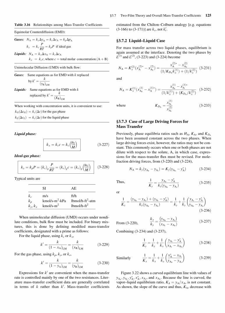
C03 09/29/2010 Page 125
Liquid phase:
kx ¼ kcc ¼ kcrLM
� ð3-227Þ
Ideal-gas phase:
ky ¼ kpP ¼ ðkcÞgP
RT¼ ðkcÞgc ¼ ðkcÞg
rGM
� ð3-228Þ
Typical units are
SI AE
kc m/s ft/h
kp kmol/s-m2-kPa lbmol/h-ft2-atm
ky, kx kmol/s-m2 lbmol/h-ft2
When unimolecular diffusion (UMD) occurs under nondi-
lute conditions, bulk flow must be included. For binary mix-
tures, this is done by defining modified mass-transfer
coefficients, designated with a prime as follows:
For the liquid phase, using kc or kx,
k0 ¼ k
ð1� xAÞLM¼ k
ðxBÞLMð3-229Þ
For the gas phase, using kp, ky, or kc,
k0 ¼ k
ð1� yAÞLM¼ k
ðyBÞLMð3-230Þ
Expressions for k0 are convenient when the mass-transfer
rate is controlled mainly by one of the two resistances. Liter-
ature mass-transfer coefficient data are generally correlated
in terms of k rather than k0. Mass-transfer coefficients
estimated from the Chilton–Colburn analogy [e.g. equations
(3-166) to (3-171)] are kc, not k0c.
§3.7.2 Liquid–Liquid Case
For mass transfer across two liquid phases, equilibrium is
again assumed at the interface. Denoting the two phases by
L(1) and L(2), (3-223) and (3-224) become
NA ¼ Kð2Þx ðxð2Þ�A � xð2ÞAbÞ ¼ x
ð2Þ�A � x
ð2ÞAb
ð1=KDAkð1Þx Þ þ ð1=kð2Þx Þ
ð3-231Þ
and
NA ¼ Kð1Þx ðxð1ÞAb� x
ð1Þ�A Þ ¼
xð1ÞAb� x
ð1Þ�A
ð1=kð1Þx Þ þ ðKDA=kð2Þx Þ
ð3-232Þ
where KDA¼ x
ð1ÞAi
xð2ÞAi
ð3-233Þ
§3.7.3 Case of Large Driving Forces forMass Transfer
Previously, phase equilibria ratios such as HA, KA, and KDA
have been assumed constant across the two phases. When
large driving forces exist, however, the ratios may not be con-
stant. This commonly occurs when one or both phases are not
dilute with respect to the solute, A, in which case, expres-
sions for the mass-transfer flux must be revised. For mole-
fraction driving forces, from (3-220) and (3-224),
NA ¼ kyðyAb� yAi
Þ ¼ KyðyAb� y�AÞ ð3-234Þ
Thus, 1
Ky
¼ yAb� y�A
kyðyAb� yAi
Þ ð3-235Þ
or
1
Ky
¼ ðyAb� yAi
Þ þ ðyAi� y�AÞ
kyðyAb� yAi
Þ ¼ 1
kyþ 1
ky
yAi� y�A
yAb� yAi
� �
ð3-236Þ
From (3-220),kx
ky¼ yAb
� yAi
� �
xAi� xAb
ð Þ ð3-237Þ
Combining (3-234) and (3-237),
1
Ky
¼ 1
kyþ 1
kx
yAi� y�A
xAi� xAb
� �ð3-238Þ
Similarly1
Kx
¼ 1
kxþ 1
ky
x�A � xAi
yAb� yAi
� �ð3-239Þ
Figure 3.22 shows a curved equilibrium line with values of
yAb; yAi
; y�A; x�A; xAi
, and xAb. Because the line is curved, the
vapor–liquid equilibrium ratio, KA ¼ yA=xA, is not constant.As shown, the slope of the curve and thus, KA, decrease with
Table 3.16 Relationships among Mass-Transfer Coefficients
Equimolar Counterdiffusion (EMD):
Gases: NA ¼ kyDyA ¼ kcDcA ¼ kpDpA
ky ¼ kcP
RT¼ kpP if ideal gas
Liquids: NA ¼ kxDxA ¼ kcDcA
kx ¼ kcc;where c ¼ total molar concentration ðAþ BÞ
Unimolecular Diffusion (UMD) with bulk flow:
Gases: Same equations as for EMD with k replaced
by k0 ¼ k
ðyBÞLMLiquids: Same equations as for EMD with k
replaced by k0 ¼ k
ðXBÞLMWhen working with concentration units, it is convenient to use:
kGðDcGÞ ¼ kcðDcÞ for the gas phasekLðDcLÞ ¼ kcðDcÞ for the liquid phase
§3.7 Two-Film Theory and Overall Mass-Transfer Coefficients 125

C03 09/29/2010 Page 126
increasing concentration of A. Denoting two slopes of the
equilibrium curve by
mx ¼yAi� y�A
xAi� xAb
� �ð3-240Þ
and my ¼yAb� yAi
x�A � xAi
� �ð3-241Þ
then substituting (3-240) and (3-241) into (3-238) and
(3-239), respectively,
1
Ky
¼ 1
kyþmx
kxð3-242Þ
and1
Kx
¼ 1
kxþ 1
mykyð3-243Þ
EXAMPLE 3.20 Absorption of SO2 into Water.
Sulfur dioxide (A) is absorbed into water in a packed column, where
bulk conditions are 50�C, 2 atm, yAb¼ 0:085, and xAb
¼ 0:001.Equilibrium data for SO2 between air and water at 50
�C are
pSO2; atm cSO2
; lbmol/ft3
0.0382 0.00193
0.0606 0.00290
0.1092 0.00483
0.1700 0.00676
Experimental values of the mass-transfer coefficients are:
Liquid phase : kc ¼ 0:18 m/h
Gas phase : kp ¼ 0:040kmol
h-m2-kPa
For mole-fraction driving forces, compute the mass-transfer flux:
(a) assuming an average Henry’s law constant and a negligible bulk-
flow effect; (b) utilizing the actual curved equilibrium line and as-
suming a negligible bulk-flow effect; (c) utilizing the actual curved
equilibrium line and taking into account the bulk-flow effect. In ad-
dition, (d) determine the magnitude of the two resistances and the
values of the mole fractions at the interface that result from part (c).
Solution
Equilibrium data are converted to mole fractions by assuming Dal-
ton’s law, yA= pA=P, for the gas and xA ¼ cA=c for the liquid. Theconcentration of liquid is close to that of water, 3.43 lbmol/ft3 or
55.0 kmol/m3. Thus, the mole fractions at equilibrium are:
ySO2xSO2
0.0191 0.000563
0.0303 0.000846
0.0546 0.001408
0.0850 0.001971
These data are fitted with average and maximum absolute deviations
of 0.91% and 1.16%, respectively, by the equation
ySO2¼ 29:74xSO2
þ 6;733x2SO2ð1Þ
Differentiating, the slope of the equilibrium curve is
m ¼ dy
dx¼ 29:74þ 13;466xSO2
ð2Þ
The given mass-transfer coefficients are converted to kx and ky by
(3-227) and (3-228):
kx ¼ kcc ¼ 0:18ð55:0Þ ¼ 9:9kmol
h-m2
ky ¼ kpP ¼ 0:040ð2Þð101:3Þ ¼ 8:1kmol
h-m2
(a) From (1) for xAb¼ 0:001; y�A ¼ 29:74ð0:001Þ þ 6;733ð0:001Þ2
¼ 0:0365. From (1) for yAb¼ 0:085, solving the quadratic
equation yields x�A ¼ 0:001975.The average slope in this range is
m ¼ 0:085� 0:0365
0:001975� 0:001¼ 49:7
Examination of (3-242) and (3-243) shows that the liquid-
phase resistance is controlling because the term in kx is
much larger than the term in ky. Therefore, from (3-243), using
m ¼ mx,
1
Kx
¼ 1
9:9þ 1
49:7ð8:1Þ ¼ 0:1010þ 0:0025 ¼ 0:1035
or Kx¼ 9:66kmol
h-m2
From (3-223),
NA ¼ 9:66ð0:001975� 0:001Þ ¼ 0:00942kmol
h-m2
(b) From part (a), the gas-phase resistance is almost negligible.
Therefore, yAi� yAb
and xAi� x�A.
From (3-241), the slope my is taken at the point yAb¼ 0:085
and x�A ¼ 0:001975 on the equilibrium line.
By (2), my ¼ 29.74 + 13,466(0.001975) ¼ 56.3. From
(3-243),
Kx ¼ 1
ð1=9:9Þ þ ½1=ð56:3Þð8:1Þ� ¼ 9:69kmol
h-m2
giving NA ¼ 0.00945 kmol/h-m2. This is a small change from
part (a).
Slo
pe m y
xA
yA
yAi
xAixAb
yAb
xA* is a fictitious xA in
equilibrium with yAb.
yA* is a fictitious yA in
equilibrium with xAb.
Slo
pe m
x
yA*
xA*
Figure 3.22 Curved equilibrium line.
126 Chapter 3 Mass Transfer and Diffusion

C03 09/29/2010 Page 127
(c) Correcting for bulk flow, from the results of parts (a) and (b),
yAb¼ 0:085; yAi
¼ 0:085; xAi¼ 0:1975; xAb
¼ 0:001;
ðyBÞLM ¼ 1:0� 0:085 ¼ 0:915; and ðxBÞLM � 0:9986
From (3-229),
k0x ¼ 9:9
0:9986¼ 9:9
kmol
h-m2and k0y ¼ 8:1
0:915¼ 8:85
kmol
h-m2
From (3-243),
Kx ¼ 1
ð1=9:9Þ þ ½1=56:3ð8:85Þ� ¼ 9:71kmol
h-m2
From (3-223),
NA ¼ 9:7ð0:001975� 0:001Þ ¼ 0:00947kmol
h-m2
which is only a very slight change from parts (a) and (b), where the
bulk-flow effect was ignored. The effect is very small because it is
important only in the gas, whereas the liquid resistance is
controlling.
(d) The relative magnitude of the mass-transfer resistances is
1=myk0y
1=k0x¼ 1=ð56:3Þð8:85Þ
1=9:9¼ 0:02
Thus, the gas-phase resistance is only 2% of the liquid-phase resist-
ance. The interface vapor mole fraction can be obtained from
(3-223), after accounting for the bulk-flow effect:
yAi¼ yAb
� NA
k0y¼ 0:085� 0:00947
8:85¼ 0:084
Similarly, xAi¼ NA
k0xþ xAb
¼ 0:00947
9:9þ 0:001 ¼ 0:00196
§3.8 MOLECULARMASS TRANSFER INTERMS OF OTHER DRIVING FORCES
Thus far in this chapter, only a concentration driving force (in
terms of concentrations, mole fractions, or partial pressures)
has been considered, and only one or two species were trans-
ferred. Molecular mass transfer of a species such as a charged
biological component may be driven by other forces besides
its concentration gradient. These include gradients in temper-
ature, which induces thermal diffusion via the Soret effect;
pressure, which drives ultracentrifugation; electrical poten-
tial, which governs electrokinetic phenomena (dielectro-
phoresis and magnetophoresis) in ionic systems like
permselective membranes; and concentration gradients of
other species in systems containing three or more compo-
nents. Three postulates of nonequilibrium thermodynamics
may be used to relate such driving forces to frictional motion
of a species in the Maxwell–Stefan equations [28, 75, 76].
Maxwell, and later Stefan, used kinetic theory in the mid- to
late-19th century to determine diffusion rates based on
momentum transfer between molecules. At the same time,
Graham and Fick described ordinary diffusion based on bi-
nary mixture experiments. These three postulates and
applications to bioseparations are presented in this section.
Application of the Maxwell–Stefan equations to rate-based
models for multicomponent absorption, stripping, and distil-
lation is developed in Chapter 12.
§3.8.1 The Three Postulates of NonequilibriumThermodynamics
This brief introduction summarizes a more detailed synopsis
found in [28].
First postulate
The first (quasi-equilibrium) postulate states that equilibrium
thermodynamic relations apply to systems not in equilibrium,
provided departures from local equilibrium (gradients) are
sufficiently small. This postulate and the second law of ther-
modynamics allow the diffusional driving force per unit vol-
ume of solution, represented by cRTdi and which moves
species i relative to a solution containing n components, to
be written as
cRTdi cirT ;Pmi þ ciVi � vi
� �rP� ri gi �Xn
k¼1vkgk
!
ð3-244ÞXn
i¼1di ¼ 0 ð3-245Þ
where di are driving forces for molecular mass transport, ci is
molar concentration, mi is chemical potential, vi is mass frac-
tion, gi are total body forces (e.g., gravitational or electrical
potential) per unit mass, Vi is partial molar volume, and ri ismass concentration, all of which are specific to species i.
Each driving force is given by a negative spatial gradient in
potential, which is the work required to move species i rela-
tive to the solution volume. In order from left to right, the
three collections of terms on the RHS of (3-244) represent
driving forces for concentration diffusion, pressure diffusion,
and forced diffusion. The term ciVi in (3-244) corresponds to
the volume fraction of species i, fi.
Second postulate
The second (linearity) postulate allows forces on species in
(3-244) to be related to a vector mass flux, ji. It states that all
fluxes in the system may be written as linear relations involv-
ing all the forces. For mass flux, the thermal-diffusion driving
force,�bi0r ln T, is added to the previous three forces to give
ji ¼ �bi0r lnT � riXn
j¼1
bij
rirjcRTdj ð3-246Þ
bij þXn
k¼1k 6¼j
bik ¼ 0 ð3-247Þ
where bi0 and bij are phenomenological coefficients (i.e.,
transport properties). The vector mass flux, ji ¼ ri(vi � v),
is the arithmetic average of velocities of all molecules of
§3.8 Molecular Mass Transfer in Terms of Other Driving Forces 127

C03 09/29/2010 Page 128
species i in a tiny volume element (vi) relative to a mass-
averaged value of the velocities of all such components in the
mixture, v ¼Pvivi. It is related to molar flux, Ji, in (3-251).
Third postulate
According to the third postulate, Onsager’s reciprocal rela-
tions—developed using statistical mechanics and supported
by data—the matrix of the bij coefficients in the flux-force
relation (3-246) are symmetric (bij ¼ bji) in the absence of
magnetic fields. These coefficients may be rewritten as multi-
component mass diffusivities D0ij
D0ij ¼ xixj
bij
cRT ¼ D0ji� � ð3-248Þ
which exhibit less composition dependency than the trans-
port properties, bij, and reduce to the more familiar binary
diffusivity of Fick’s Law, DAB, for ideal binary solutions, as
shown in Figure 3.23, and illustrated in Example 3.21.
§3.8.2 Maxwell–Stefan Equations
To show the effects of forces on molecular motion of species
i, (3-248) is substituted into (3-246), which is solved for the
driving forces, di, and set equal to (3-244). Using ji ¼ ri(vi �v), discussed above, a set of n � 1 independent rate expres-
sions, called theMaxwell–Stefan equations, is obtained:
Xn
j¼1
xixj
D0ijvi � vj� � ¼ 1
cRT
"cirT ;Pmi þ fi � við ÞrP
� ri gi �Xn
k¼1vkgk
!#�Xn
j¼1
xixj
D0ij
bi0
ri� bj0
rj
!r lnT
ð3-249Þ
The set of rate expressions given by (3-249) shows molec-
ular mass transport of species i driven by gradients in
pressure, temperature, and concentration of species i for j 6¼ i
in systems containing three or more components, as well as
driven by body forces that induce gradients in potential. The
total driving force for species i due to potential gradients col-
lected on the LHS of (3-249) is equal to the sum on the RHS
of the cumulative friction force exerted on species i—zi,jxj(xi � xj)—by every species j in a mixture, where frictional
coefficient zij is given by xi=D0ij in (3-249). The friction
exerted by j on i is proportional to the mole fraction of j in
the mixture and to the difference in average molecular veloc-
ity between species j and i.
Body forces in (3-249) may arise from gravitational accel-
eration, g; electrostatic potential gradients, rw, or mechani-
cally restraining matrices (e.g., permselective membranes
and friction between species i and its surroundings), denoted
by dim. These can be written as
gi ¼ g� zi=Mi
� �rwþ dim
1
rmrP ð3-250Þ
where zi is elementary charge and Faraday’s constant, =, ¼96,490 absolute coulombs per gram-equivalent.
Chemical versus physical potentials
Potential can be defined as the reversible work required to
move an entity relative to other elements in its surroundings.
The change in potential per unit distance provides the force
that drives local velocity of a species relative to its environ-
ment in (3-249). For molecules, potential due to gravity in
(3-250)—an external force that affects the whole system—is
insignificant relative to chemical potential in (3-249), an in-
ternal force that results in motion within the system but not
in the system as whole. Gravity produces a driving force
downward at height z, resulting from a potential difference
due to the work performed to attain the height, �mgDz,divided by the height, Dz, which reduces to mg. For gold
(a dense molecule), this driving force ¼ ð0:197 kg/molÞð10 m/s2Þ ffi 2 N/mol. Gravitational potential of gold across
the distance of a centimeter is therefore 2 � 10�2 N/mol.
Chemical potential can be defined as the reversible work
needed to separate one mole of species i from a large amount
of a mixture. Its magnitude increases logarithmically with the
species activity, or Dm ¼ �RTD ln(gixi). Gold, in an ideal
solution (gi ¼ 1) and for ambient conditions at xi ¼ 1/e ¼0.368, experiences a driving force times distance due to
a chemical potential of �(8.314 J/mol–K)(298 K) � ln
(0.37) ¼ 2,460 J/mol. The predominance of chemical poten-
tial leads to an approximate linear simplification of (3-249)—
which neglects potentials due to pressure, temperature, and
external body forces—that is applicable in many practical sit-
uations, as illustrated later in Example 3.25. Situations in
which the other potentials are significant are also considered.
For instance, Example 3.21 below shows that ultra-
centrifugation provides a large centripetal (‘‘center-seek-
ing’’) force to induce molecular momentum, rP, sufficientto move species i in the positive direction, if its mass fraction
is greater than its volume fraction (i.e., if component i is
denser than its surroundings).
2.0
Mole fraction ether
Act
ivit
y
1.00 1.0
2.5
D’AB
DAB
Figure 3.23 Effect of activity on the product of viscosity and
diffusivity for liquid mixtures of chloroform and diethyl ether [R.E.
Powell, W.E. Roseveare, and H. Eyring, Ind. Eng. Chem., 33, 430–
435 (1941)].
128 Chapter 3 Mass Transfer and Diffusion

C03 09/29/2010 Page 129
Driving forces for species velocities
Effects of driving forces on species velocity are illustrated in
the following seven examples reduced from [28], [75], [76],
and [77]. These examples show how to apply (3-249) and
(3-250), together with species equations of continuity, the
equation of motion, and accompanying auxiliary (bootstrap)
relations such as (3-245) and (3-248). The auxiliary expres-
sions are needed to provide the molecular velocity of the se-
lected reference frame because the velocities in (3-249) are
relative values. The first example considers concentration-
driving forces in binary systems. Measured data for D0ij, whichrequires simultaneous measurement of gi as a function of xi,
are rare. Instead, the multicomponent diffusivity values may
be estimated from phenomenological Fick’s law diffusivities.
EXAMPLE 3.21 Maxwell–Stefan Equations Related to
Fick’s Law.
Consider a binary system containing species A and B that is iso-
tropic in all but concentration [75]. Show the correspondence
between DAB and D0AB by relating (3-249) to the diffusive molar
flux of species A relative to the molar-average velocity of a mixture,
JA, which may be written in terms of the mass-average velocity, jA:
JA ¼ �cDABrxA ¼ cA vA � vMð Þ ¼ jAcxAxB
rvAvB
ð3-251Þ
where vM ¼ xAvAþ xBvB is the molar-average velocity of a
mixture.
Solution
In a binary system, xB ¼ 1 � xA, and the LHS of (3-249) may be
written as
xAxB
D0ABvB � vAð Þ ¼ xA
D0ABxBvB þ xAvA � vAð Þ ¼ � xA
D0ABJA
cA
ð3-252Þwhich relates the friction force to the molar flux. Substitutingrmi ¼RTrln(ai) into the RHS of (3-249), setting it equal to (3-252), and
rearranging, gives
JA ¼ �cD0AB xAr ln aA þ 1
cRTfA � vAð ÞrP½
�
�rvAvB gA � gBð Þ� þ kTr ln Tg ð3-253Þ
kT ¼ bA0
rD0AB
xAxB
vAvB
¼ aTxAxB ¼ sTxAxBT ð3-254Þ
Equation (3-253) describes binary diffusion in gases or liquids. It is
a specialized form of the generalized Fick equations. Equation (3-
254) relates the thermal diffusion ratio, kT, to the thermal diffusion
factor, aT, and the Soret coefficient, sT. For liquids, sT is preferred.
For gases, aT is nearly independent of composition.
Table 3.17 shows concentration- and temperature-dependent kTvalues for several binary gas and liquid pairs. Species A moves to
the colder region when the value of kT is positive. This usually cor-
responds to species A having a larger molecular weight (MA) or
diameter. The sign of kT may change with temperature.
In this example, the effects of pressure, thermal diffusion, and
body force terms in (3-253) may be neglected. Then from the
properties of logarithms,
xAr ln aA ¼ rxA þ xAr ln gA ¼ rxA 1þ q ln gAq ln xA
� �ð3-255Þ
By substituting (3-255) into (3-253) and comparing with (3-251), it
is found that
DAB ¼ 1þ q ln gAq ln xA
� �D0AB ð3-256Þ
The activity-based diffusion coefficient D0AB is less concentration-
dependent than DAB but requires accurate activity data, so it is used
less widely. Multicomponent mixtures of low-density gases have
gi ¼ 1 and di ¼ rxi for concentration diffusion and DAB ¼ D0ABfrom kinetic theory.
EXAMPLE 3.22 Diffusion via a Thermal Gradient
(thermal diffusion).
Consider two bulbs connected by a narrow, insulated tube that are
filled with a binary mixture of ideal gases [28]. (Examples of binary
mixtures are given in Table 3.17.) Maintaining the two bulbs at con-
stant temperatures T2 and T1, respectively, typically enriches the
larger species at the cold end for a positive value of kT. Derive an
expression for (xA2 � xA1), the mole-fraction difference between
the two bulbs, as a function of kT, T2, and T1 at steady state, neglec-
ting convection currents in the connecting tube.
Solution
There is no net motion of either component at steady state, so JA ¼0. Use (3-253) for the ideal gases (gA ¼ 1), setting the connecting
tube on the z-axis, neglecting pressure and body forces, and apply-
ing the properties of logarithms to obtain
dxA
dz¼ � kT
T
dT
dzð3-257Þ
Table 3.17 Experimental Thermal Diffusion Ratios for
Low-Density Gas and Liquid Mixtures
Species A-B T(K) xA kT {xA,T}
Gas
Ne-He 330 0.80 0.0531
0.40 0.1004
N2-H2 264 0.706 0.0548
0.225 0.0663
D2-H2 327 0.90 0.1045
0.50 0.0432
0.10 0.0166
Liquid
C2H2Cl4-n-C6H14 298 0.5 1.08
C2H4Br2-C2H4Cl2 298 0.5 0.225
C2H2Cl4-CCl4 298 0.5 0.060
CBr4-CCl4 298 0.09 0.129
CCl4-CH3OH 313 0.5 1.23
CH3OH-H2O 313 0.5 �0.137Cyclo-C6H12-C6H6 313 0.5 0.100
Data from Bird et al. [28].
§3.8 Molecular Mass Transfer in Terms of Other Driving Forces 129

C03 09/29/2010 Page 130
The integral of (3-257) may be evaluated by neglecting composition
effects on kT for small differences in mole fraction and using a value
of kT at a mean temperature, Tm, to yield
xA2 � xA1 ¼ �kT Tmf gln T2
T1
ð3-258Þ
where the mean temperature at which to evaluate kT is
Tm ¼ T1T2
T2 � T1
lnT2
T1
ð3-259Þ
Substituting values of kT from Table 3.17 into (3-258) suggests that
a very large temperature gradient is required to obtain more than a
small composition difference. During World War II, uranium iso-
topes were separated in cascades of Clausius–Dickel columns based
on thermal diffusion between sets of vertical heated and cooled
walls. The separation supplemented thermal diffusion with free con-
vection to allow species A, enriched at the cooled wall, to descend
and species B, enriched at the heated wall, to ascend. Energy expen-
ditures were enormous.
EXAMPLE 3.23 Diffusion via a Pressure Gradient
(pressure diffusion).
Components A and B in a small cylindrical tube of length L, held at
radial position Ro� L inside an ultracentrifuge, are rotated at con-
stant angular velocity V [28]. The species experience a change in
molecular momentum, rp, due to centripetal (‘‘center-seeking’’)
acceleration gV ¼ V2r given by the equation of motion,
dp
dr¼ rgV ¼ rV2r ¼ r
v2ur
ð3-260Þ
where vu¼ duVr is the linear velocity. Derive expressions for (1) the
migration velocity, vmigr, of dilute A in B (e.g., protein in H2O) in
terms of relative molecular weight, and for (2) the distribution of
the two components at steady state in terms of their partial molar
volumes, �Vi , i ¼ A, B, and the pressure gradient, neglecting changes
in �Vi and gi over the range of conditions in the centrifuge tube.
Solution
The radial motion of species A is obtained by substituting (3-255)
into the radial component of the binary Maxwell–Stefan equation in
(3-253) for an isothermal tube free of external body forces to give
JA ¼ �cD0AB 1þ qlngAqlnxA
� �dxA
drþ 1
cRTfA � vAð Þ dP
dr
� �ð3-261Þ
where the pressure gradient of the migration term in (3-261) remains
relatively constant in the tube since L � Ro. Molecular-weight de-
pendence in this term in the limit of a dilute solution of protein (A)
in H2O (B) arises in the volume and mass fractions, respectively,
wA ¼ cAVA ¼ xAcVA � xAVA
VB
¼ xAMA
MB
V̂A
V̂B
ð3-262Þ
vA ¼ rAr¼ cAMA
cM¼ xA
MA
xAMA þ xBMB
� xAMA
MB
ð3-263Þ
where V̂ i ¼ �Vi=Mi is the partial specific volume of species i, which
is 1 mL/g for H2O and �0.75 mL/g for a globular protein (see Table
3.18). A pseudo-binary Fickian diffusivity given by (3-256) to be
substituted into (3-261) may be estimated using Stokes law:
DAB ¼ kT
6pmBRAfAð3-264Þ
where RA is the radius of a sphere whose volume equals that of the
protein, and protein nonsphericity is accounted for by a hydro-
dynamic shape factor, fA. Substituting (3-256), (3-260), (3-262), and
(3-263) into (3-261) gives
JA ¼ �cDAB
dxA
drþ cA �D0AB
cRT
MA
MB
V̂A
V̂B
� 1
� �� �rV2r
� ð3-265Þ
where the term inside the curly brackets on the RHS of (3-265) cor-
responds to the migration velocity, vmigr, in the +r direction driven
by centripetal force in proportion to the relative molecular weight,
MA=MB. The ratio of vmigr to centripetal force in (3-265) is the sedi-
mentation coefficient, s, which is typically expressed in Svedberg
(S) units (1 S ¼ 10�13 sec), named after the inventor of the ultra-
centrifuge. Protein molecular-weight values obtained by photo-
electric scanning detection of vmigr to determine s in pure water (w)
at 20� (i.e., s20,w) are summarized in Table 3.18. Equation (3-265) is
the basis for analyzing transient behavior, steady polarization, and
preparative application of ultracentrifugation.
Concentration and pressure gradients balance at steady state
(JA ¼ 0), and with constant �Vi and gi in the tube and xA � xB lo-
cally, writing (3-253) for species A gives
0 ¼ dxA
drþMAxA
RT
VA
MA
� 1
r
� �dp
drð3-266Þ
Multiplying (3-266) by ð�VB=xAÞdr, and substituting a constant cen-
tripetal force (r � Ro) from (3-260), gives
VB
dxA
xA¼ VB
gVRT
rVA �MA
� �dr ð3-267Þ
Writing an equation analogous to (3-267) for species B, and sub-
tracting it from (3-267), gives
VB
dxA
xA� VA
dxB
xB¼ gV
RTMAVB �MBVA
� �dr ð3-268Þ
Integrating (3-268) from xi{r ¼ 0} ¼ xi0 to xi{r} for i ¼ A,B, using
r ¼ 0 at the distal tube end, gives
VB lnxA
xA0� VA ln
xB
xB0¼ gV
RTMBVA �MAVB
� �r ð3-269Þ
Table 3.18 Protein Molecular Weights Determined by
Ultracentrifugation
Protein M s20,w (S)
V2
(cm3g�1)
Ribonuclease (bovine) 12,400 1.85 0.728
Lysozyme (chicken) 14,100 1.91 0.688
Serum albumin
(bovine)
66,500 4.31 0.734
Hemoglobin 68,000 4.31 0.749
Tropomysin 93,000 2.6 0.71
Fibrinogen (human) 330,000 7.6 0.706
Myosin (rod) 570,000 6.43 0.728
Bushy stunt virus 10,700,000 132 0.74
Tobacco mosaic virus 40,000,000 192 0.73
Data from Cantor and Schimmel [78].
130 Chapter 3 Mass Transfer and Diffusion

C03 09/29/2010 Page 131
Using the properties of logarithms and taking the exponential of
both sides of (3-269) yields the steady-state species distribution in
terms of the partial molar volumes:
xA
xA0
� �VB xB0
xB
� �VA
¼ expgVr
RTMBVA �MAVB
� �h ið3-270Þ
The result in (3-269) is independent of transport coefficients and
may thus be obtained in an alternative approach using equilibrium
thermodynamics.
EXAMPLE 3.24 Diffusion in a Ternary System via
Gradients in Concentration and Electrostatic Potential.
A 1-1 electrolyte M+X� (e.g., NaCl) diffuses in a constriction bet-
ween two well-mixed reservoirs at different concentrations contain-
ing electrodes that exhibit a potential difference, Dw, measured by a
potentiometer under current-free conditions [75]. Derive an expres-
sion for salt flux in the system.
Solution
Any pressure difference between the two reservoirs is negligible rel-
ative to the reference pressure, cRT � 1,350 atm, at ambient condi-
tions. Electroneutrality, in the absence of current flow through the
potentiometer, requires that
xMþ ¼ xX� ¼ xS ¼ 1� xW ð3-271Þ
NMþ ¼ NX� ¼ NS ð3-272ÞSubstituting (3-271) into (3-249) and rearranging yields the n � 1
Maxwell–Stefan relations:
1
cD0MþWxWNMþ � xMþNWð Þ
¼ �xMþrT;PaMþ þrMþ
cRTgMþ �
Xn
k¼1vkgk
!ð3-273Þ
1
cD0X�WxWNX� � xX�NWð Þ
¼ �xX�rT;PaX� þ rX�
cRTgX� �
Xn
k¼1vkgk
!ð3-274Þ
No ion-ion diffusivity appears because vMþ � vX� ¼ 0 in the
absence of current. Substituting (3-250), (3-271), and (3-272) into
(3-273) and (3-274) and rearranging yields
1
cD0MþWxWNS � xSNWð Þ ¼ � q ln aMþ
q ln xSrxS � xS
RT=rw ð3-275Þ
1
cD0X�WxWNS � xSNWð Þ ¼ � q ln aX�
q ln xSrxS þ xS
RT=rw ð3-276Þ
Adding (3-275) and (3-276) eliminates the electrostatic potential, to
give
NS ¼ � 1
cD0MþWþ 1
cD0X�W
� ��1 q ln aMþaX�ð Þq ln xS
rxS þ xS NS þ NWð Þ
ð3-277Þwhich has the form of Fick’s law after a concentration-based diffusiv-
ity is defined:
DSW ¼ 2D0MþWD0X�W
D0MþW þ D0X�W
� �1þ q lngS
q lnxS
� �ð3-278Þ
gS ¼ gMþgX� ð3-279Þwhere gS is the mean activity coefficient given by aS ¼ aM þ aX�¼ x2s ½ðgM þ gX�Þ1=2�2 ¼ x2s ½ðgSÞ1=2�2. Equation (3-278) shows that
while fast diffusion of small counterions creates a potential gradient
that speeds large ions, the overall diffusivity of the salt pair is domi-
nated by the slower ions (e.g., proteins).
EXAMPLE 3.25 Film Mass Transfer.
Species velocity in (3-249) is due to (1) bulk motion; (2) gradient of
a potential Dci ¼ cid � cio of species i across distance d (which
moves species i relative to the mixture); and (3) friction between
species and surroundings [77]. Develop an approximate expression
for film mass transfer using linearized potential gradients.
Solution
The driving force that results from the potential gradient, �dci=dz,is approximated by the difference in potential across a film of thick-
ness d, �Dci=d. Linearizing the chemical potential difference by
Dmi ¼ RTDln gixið Þ � RTxid � xio
xid þ xioð Þ=2 ¼ RTDxi�xi
ð3-280Þ
provides a tractable approximation that has reasonable accuracy
over a wide range of compositions [77].
Friction from hydrodynamic drag of fluid (1) of viscosity m1 on a
spherical particle (2) of diameter d2 is proportional to their relative
difference in velocity, v, viz.,
� dm2
dz¼ 3NApm1 v2 � v1ð Þd2 ð3-281Þ
where NA (Avogadro’s number) represents particles per mole. A
large force is produced when the drag is summed over a mole of
particles.
Rearranging (3-281) yields an expression for the Maxwell–
Stefan diffusivity in terms of hydrodynamic drag:
� d
dz
m2
RT
� ¼ v2 � v1
D012ð3-282Þ
D012 ¼ RT
NA3ph1d2
ð3-283Þ
Substituting (3-280) into (3-282) and rearranging, after linearizing
the derivative across a film of thickness d, yields the mass transport
coefficient, k12,
Dx2�x2¼ �v1 � �v2
k12ð3-284Þ
k12 ¼ D012d
ð3-285Þ
where kij is �10�1 m/s for gases and 10�4 m/s for liquids. These
values decrease by approximately a factor of 10 for gases and
liquids in porous media.
In a general case that includes any number of components, fric-
tion between components j and i per mole of i is proportional to the
difference between the mean velocities of j and i, respectively.
§3.8 Molecular Mass Transfer in Terms of Other Driving Forces 131

C03 09/29/2010 Page 132
Taking friction proportional to the local concentration of j decreases
the composition dependence of kij, viz.,
�xj�vj � �vikij
ð3-286Þ
Because assigning a local concentration to a component like a solid
membrane component, m, is difficult, a membrane coefficient, ki,
may be introduced instead:
�xmkim¼ 1
kið3-287Þ
§3.8.3 Maxwell–Stefan Difference Equation
Linearization allows application of a difference form of the
Maxwell–Stefan equation, which is obtained by setting the
negative driving force on species i equal to the friction on
species i, viz. [77]:
Dxi�xiþ ::: ¼
X
j
�xj�vj � �vikij
ð3-288Þ
where the ellipsis . . . allows addition of relevant linearized
potentials in addition to the chemical potential. The accuracy
of (3-288) is adequate for many engineering calculations.
This is illustrated by determining molar solute flux of dilute
and nondilute solute during binary stripping, and by estimat-
ing concentration polarization and permeate flux in tangen-
tial-flow filtration.
Dilute stripping
Consider stripping a trace gas (1) ð�x2 � 1Þ from a liquid through
a gas film into an ambient atmosphere. The atmosphere is taken
at a reference velocity (v2¼ 0). Application of (3-288) yields
k12Dx1�x1¼ ��v1 ð3-289Þ
or N1 ¼ c�v1�x1 ¼ �ck12Dx1 ð3-290ÞThe result in (3-290), obtained from the Maxwell–Stefan dif-
ference equation, is consistent with (3-35) for dilute (x2 �1)solutions, which was obtained from Fick’s law.
Nondilute stripping
For this situation, �x1 ¼ 0:5 ¼ �x2, and drift occurs in the gas
film. From (3-288),
k12Dx1�x1¼ �0:5 � �v1 ð3-291Þ
for which
N1 ¼ c�v1�x1 ¼ �2ck12Dx1 ð3-292ÞThe latter result is easily obtained using (3-288) without
requiring a drift-correction, as Fick’s law would have.
Concentration polarization in tangential flow filtration
Now consider the flux of water (2) through a semipermeable
membrane that completely retains a dissolved salt (1) at
dilute concentration (x2 � 1), as discussed in [77]. Set the
velocity of the salt equal to a stationary value in the frame of
reference (v1 ¼ 0). The average salt concentration in a film of
thickness d adjacent to the membrane is
�x1 ¼ x1o þ x1d � x1o
2¼ x1o þ Dx1
2ð3-293Þ
Using (3-288) gives
k12Dx1�x1¼ �v2 ð3-294Þ
Combining (3-293) and (3-294) gives the increase in salt con-
centration in the film relative to its value in the bulk:
Dx1x1o¼
2�v2k12
2� �v2k12
ð3-295Þ
EXAMPLE 3.26 Flux in Tangential-Flow Filtration.
Relate flux of permeate, j, in tangential-flow filtration to local wall
concentration of a completely retained solute, i, using the Maxwell–
Stefan difference equation.
Solution
Local permeate flux is given by Nj ¼ �cj�vj. An expression for local
water velocity is obtained by solving (3-295) for �vj:
�vj ¼ kijDxi
Dxi=2þ xi;b� kij ln
xi;w
xi;bð3-296Þ
where subscripts b and w represent bulk feed and wall, respectively.
In a film, kij ¼ Dij=d. Local permeate flux is then
Nj ¼ cjDij
dlnxi;w
xi;bð3-297Þ
The result is consistent with the classical stagnant-film model in
(14-108), which was obtained using Fick’s law.
EXAMPLE 3.27 Maxwell–Stefan Difference
Equations Related to Fick’s Law.
For a binary system containing species A and B, show how DAB re-
lates to D0AB in the Maxwell–Stefan difference equation by relating
(3-288) with the diffusive flux of species A relative to the molar-av-
erage velocity of a mixture in (3-3a),
JAz¼ �DAB
dcA
dz¼ cA vA � vMð Þ ð3-298Þ
where vM ¼ xAvA þ xBvB is the molar-average velocity of a
mixture.
Solution
For a binary system, (3-288) becomes
1
xA
dxA
dz¼ �xB
�vB � �vAD0AB
¼ �xB�vB þ �xA�vA � �vAD0AB
¼ � �vA � vM
D0ABð3-299Þ
132 Chapter 3 Mass Transfer and Diffusion
C03 09/29/2010 Page 133
Comparing (3-298) and (3-299) shows that for the Maxwell–
Stefan difference equation
D0AB ¼ DAB ð3-300ÞThe result in (3-300) is consistent with kinetic theory for multi-
component mixtures of low-density gases, for which gi ¼ 1 and di¼ rxi for concentration diffusion.
This abbreviated introduction to the Maxwell–Stefan rela-
tions has shown how this kinetic formulation yields diffusive
flux of species proportional to its concentration gradient like
Fick’s law for binary mixtures, and provides a basis for exam-
ining molecular motion in separations based on additional
driving forces such as temperature, pressure, and body forces.
For multicomponent mixtures that are typical of biosepara-
tions, the relations also quantitatively identify how the flux of
each species affects the transport of any one species. This ap-
proach yields concentration gradients of each species in terms
of the fluxes of the other species, which often requires expen-
sive computational inversion. Fick’s law may be generalized
to obtain single-species flux in terms of concentration gradi-
ents for all species, but the resulting Fickian multicomponent
diffusion coefficients are conjugates of the binary diffusion
coefficients. The linearized Maxwell–Stefan difference equa-
tion allows straightforward analysis of driving forces due
to concentration-, pressure-, body force-, and temperature-
driving forces in complex separations like bioproduct purifica-
tion, with accuracy adequate for many applications.
SUMMARY
1. Mass transfer is the net movement of a species in a mix-
ture from one region to a region of different concentra-
tion, often between two phases across an interface. Mass
transfer occurs by molecular diffusion, eddy diffusion,
and bulk flow. Molecular diffusion occurs by a number
of different driving forces, including concentration (ordi-
nary), pressure, temperature, and external force fields.
2. Fick’s first law for steady-state diffusion states that the
mass-transfer flux by ordinary molecular diffusion is
equal to the product of the diffusion coefficient (diffusiv-
ity) and the concentration gradient.
3. Two limiting cases of mass transfer in a binary mixture are
equimolar counterdiffusion (EMD) and unimolecular dif-
fusion (UMD). The former is also a good approximation
for distillation. The latter includes bulk-flow effects.
4. When data are unavailable, diffusivities (diffusion coef-
ficients) in gases and liquids can be estimated. Diffusivi-
ties in solids, including porous solids, crystalline solids,
metals, glass, ceramics, polymers, and cellular solids,
are best measured. For some solids, e.g., wood, diffusiv-
ity is anisotropic.
5. Diffusivities vary by orders of magnitude. Typical values
are 0.10, 1 � 10�5, and 1 � 10�9 cm2/s for ordinary
molecular diffusion of solutes in a gas, liquid, and solid,
respectively.
6. Fick’s second law for unsteady-state diffusion is readily
applied to semi-infinite and finite stagnant media,
including anisotropic materials.
7. Molecular diffusion under laminar-flow conditions is de-
termined from Fick’s first and second laws, provided
velocity profiles are available. Common cases include
falling liquid-film flow, boundary-layer flow on a flat
plate, and fully developed flow in a straight, circular
tube. Results are often expressed in terms of a mass-
transfer coefficient embedded in a dimensionless group
called the Sherwood number. The mass-transfer flux is
given by the product of the mass-transfer coefficient and
a concentration-driving force.
8. Mass transfer in turbulent flow can be predicted by anal-
ogy to heat transfer. The Chilton–Colburn analogy uti-
lizes empirical j-factor correlations with a Stanton
number for mass transfer. A more accurate equation by
Churchill and Zajic should be used for flow in tubes, par-
ticularly at high Reynolds numbers.
9. Models are available for mass transfer near a two-fluid
interface. These include film theory, penetration theory,
surface-renewal theory, and the film-penetration theory.
These predict mass-transfer coefficients proportional to
the diffusivity raised to an exponent that varies from 0.5
to 1.0. Most experimental data provide exponents rang-
ing from 0.5 to 0.75.
10. Whitman’s two-film theory is widely used to predict the
mass-transfer flux from one fluid, across an interface,
and into another fluid, assuming equilibrium at the inter-
face. One resistance is often controlling. The theory
defines an overall mass-transfer coefficient determined
from the separate coefficients for each of the phases and
the equilibrium relationship at the interface.
11. The Maxwell–Stefan relations express molecular motion
of species in multicomponent mixtures in terms of
potential gradients due to composition, pressure, temper-
ature, and body forces such as gravitational, centripetal,
and electrostatic forces. This formulation is useful to
characterize driving forces in addition to chemical
potential, that act on charged biomolecules in typical
bioseparations.
REFERENCES
1. Taylor, R., and R. Krishna,Multicomponent Mass Transfer, John Wiley
& Sons, New York (1993).
2. Poling, B.E., J.M. Prausnitz, and J.P. O’Connell, The Properties of
Liquids and Gases, 5th ed., McGraw-Hill, New York (2001).
References 133

C03 09/29/2010 Page 134
3. Fuller, E.N., P.D. Schettler, and J.C. Giddings, Ind. Eng. Chem.,
58(5), 18–27 (1966).
4. Takahashi, S., J. Chem. Eng. Jpn., 7, 417–420 (1974).
5. Slattery, J.C., M.S. thesis, University of Wisconsin, Madison (1955).
6. Wilke, C.R., and P. Chang, AIChE J., 1, 264–270 (1955).
7. Hayduk, W., and B.S. Minhas, Can. J. Chem. Eng., 60, 295–299
(1982).
8. Quayle, O.R., Chem. Rev., 53, 439–589 (1953).
9. Vignes, A., Ind. Eng. Chem. Fundam., 5, 189–199 (1966).
10. Sorber, H.A., Handbook of Biochemistry, Selected Data for Molecular
Biology, 2nd ed., Chemical Rubber Co., Cleveland, OH (1970).
11. Geankoplis, C.J., Transport Processes and Separation Process Princi-
ples, 4th ed., Prentice-Hall, Upper Saddle River, NJ (2003).
12. Friedman, L., and E.O. Kraemer, J. Am. Chem. Soc., 52, 1298–1314,
(1930).
13. Boucher, D.F., J.C. Brier, and J.O. Osburn, Trans. AIChE, 38, 967–993
(1942).
14. Barrer, R.M., Diffusion in and through Solids, Oxford University Press,
London (1951).
15. Swets, D.E., R.W., Lee, and R.C Frank, J. Chem. Phys., 34, 17–22
(1961).
16. Lee, R.W., J. Chem, Phys., 38, 448–455 (1963).
17. Williams, E.L., J. Am. Ceram. Soc., 48, 190–194 (1965).
18. Sucov, E.W, J. Am. Ceram. Soc., 46, 14–20 (1963).
19. Kingery, W.D., H.K. Bowen, and D.R. Uhlmann, Introduction to
Ceramics, 2nd ed., John Wiley & Sons, New York (1976).
20. Ferry, J.D., Viscoelastic Properties of Polymers, John Wiley & Sons,
New York (1980).
21. Rhee, C.K., and J.D. Ferry, J. Appl. Polym. Sci., 21, 467–476 (1977).
22. Brandrup, J., and E.H. Immergut, Eds., Polymer Handbook, 3rd ed.,
John Wiley & Sons, New York (1989).
23. Gibson, L.J., and M.F. Ashby, Cellular Solids, Structure and Propert-
ies, Pergamon Press, Elmsford, NY (1988).
24. Stamm, A.J., Wood and Cellulose Science, Ronald Press, New York
(1964).
25. Sherwood, T.K., Ind. Eng. Chem., 21, 12–16 (1929).
26. Carslaw, H.S., and J.C. Jaeger, Heat Conduction in Solids, 2nd ed.,
Oxford University Press, London (1959).
27. Crank, J., The Mathematics of Diffusion, Oxford University Press, Lon-
don (1956).
28. Bird, R.B., W.E. Stewart, and E.N. Lightfoot, Transport Phenomena,
2nd ed., John Wiley & Sons, New York (2002).
29. Churchill, R.V., Operational Mathematics, 2nd ed., McGraw-Hill, New
York (1958).
30. Abramowitz, M., and I. A. Stegun, Eds., Handbook of Mathematical
Functions, National Bureau of Standards, Applied Mathematics Series 55,
Washington, DC (1964).
31. Newman, A.B., Trans. AIChE, 27, 310–333 (1931).
32. Grimley, S.S., Trans. Inst. Chem. Eng. (London), 23, 228–235 (1948).
33. Johnstone, H.F., and R.L. Pigford, Trans. AIChE, 38, 25–51 (1942).
34. Olbrich, W.E., and J.D. Wild, Chem. Eng. Sci., 24, 25–32 (1969).
35. Churchill, S.W., The Interpretation and Use of Rate Data: The Rate
Concept, McGraw-Hill, New York (1974).
36. Churchill, S.W., and R. Usagi, AIChE J., 18, 1121–1128 (1972).
37. Emmert, R.E., and R.L. Pigford, Chem. Eng. Prog., 50, 87–93 (1954).
38. Prandtl, L., Proc. 3rd Int. Math. Congress, Heidelberg (1904);
reprinted in NACA Tech. Memo 452 (1928).
39. Blasius, H., Z. Math Phys., 56, 1–37 (1908) reprinted in NACA Tech.
Memo 1256 (1950).
40. Schlichting, H., Boundary Layer Theory, 4th ed., McGraw-Hill, New
York (1960).
41. Pohlhausen, E., Z. Angew. Math Mech., 1, 252 (1921).
42. Pohlhausen, E., Z. Angew. Math Mech., 1, 115–121 (1921).
43. Langhaar, H.L., Trans. ASME, 64, A–55 (1942).
44. Graetz, L., Ann. d. Physik, 25, 337–357 (1885).
45. Sellars, J.R., M. Tribus, and J.S. Klein, Trans. ASME, 78, 441–448
(1956).
46. Leveque, J., Ann. Mines, [12], 13, 201, 305, 381 (1928).
47. Knudsen, J.G., and D.L. Katz, Fluid Dynamics and Heat Transfer,
McGraw-Hill, New York (1958).
48. Hausen, H., Verfahrenstechnik Beih. z. Ver. Deut. Ing., 4, 91 (1943).
49. Linton, W.H., Jr., and T.K. Sherwood, Chem. Eng. Prog., 46, 258–264
(1950).
50. Reynolds, O., Trans. Roy. Soc. (London), 174A, 935–982 (1883).
51. Boussinesq, J.,Mem. Pre. Par. Div. Sav., XXIII, Paris (1877).
52. Prandtl, L., Z. Angew, Math Mech., 5, 136 (1925); reprinted in NACA
Tech. Memo 1231 (1949).
53. Reynolds, O., Proc. Manchester Lit. Phil. Soc., 14, 7 (1874).
54. Colburn, A.P., Trans. AIChE, 29, 174–210 (1933).
55. Chilton, T.H., and A.P. Colburn, Ind. Eng. Chem., 26, 1183–1187
(1934).
56. Prandtl, L., Physik. Z., 11, 1072 (1910).
57. Friend, W.L., and A.B. Metzner, AIChE J., 4, 393–402 (1958).
58. Nernst, W., Z. Phys. Chem., 47, 52 (1904).
59. Higbie, R., Trans. AIChE, 31, 365–389 (1935).
60. Danckwerts, P.V., Ind. Eng. Chem., 43, 1460–1467 (1951).
61. Levenspiel, O., Chemical Reaction Engineering, 3rd ed., John Wiley &
Sons, New York (1999).
62. Toor, H.L., and J.M. Marchello, AIChE J., 4, 97–101 (1958).
63. Whitman, W.G., Chem. Met. Eng., 29, 146–148 (1923).
64. van Driest, E.R., J. Aero Sci., 1007–1011, 1036 (1956).
65. Reichardt, H., Fundamentals of Turbulent Heat Transfer, NACA Report
TM-1408 (1957).
66. Drew, T.B., E.C. Koo, and W.H. McAdams, Trans. Am. Inst. Chem.
Engrs., 28, 56 (1933).
67. Nikuradse, J., VDI-Forschungsheft, p. 361 (1933).
68. Launder, B.E., and D.B. Spalding, Lectures in Mathematical Models of
Turbulence, Academic Press, New York (1972).
69. Heng, L., C. Chan, and S.W. Churchill, Chem. Eng. J., 71, 163 (1998).
70. Churchill, S.W., and S.C. Zajic, AIChE J., 48, 927–940 (2002).
71. Churchill, S.W., ‘‘Turbulent Flow and Convection: The Prediction of
Turbulent Flow and Convection in a Round Tube,’’ in J.P. Hartnett and T.F.
Irvine, Jr., Ser. Eds., Advances in Heat Transfer, Academic Press, New York,
Vol. 34, pp. 255–361 (2001).
72. Yu, B., H. Ozoe, and S.W. Churchill, Chem. Eng. Sci., 56, 1781 (2001).
73. Churchill, S.W., and C. Chan, Ind. Eng. Chem. Res., 34, 1332 (1995).
74. Churchill, S.W., AIChE J., 43, 1125 (1997).
75. Lightfoot, E.N., Transport Phenomena and Living Systems, John Wiley
& Sons, New York (1974).
134 Chapter 3 Mass Transfer and Diffusion

C03 09/29/2010 Page 135
76. Taylor, R., and R. Krishna,Multicomponent Mass Transfer, John Wiley
& Sons, New York (1993).
77. Wesselingh, J.A., and R. Krishna, Mass Transfer in Multicomponent
Mixtures, Delft University Press, Delft (2000).
78. Cantor, C.R., and P.R. Schimmel, Biophysical Chemistry Part II. Tech-
niques for the study of biological structure and function, W.H. Freeman and
Co., New York (1980).
STUDY QUESTIONS
3.1. What is meant by diffusion?
3.2. Molecular diffusion occurs by any of what four driving forces
or potentials? Which one is the most common?
3.3. What is the bulk-flow effect in mass transfer?
3.4. How does Fick’s law of diffusion compare to Fourier’s law of
heat conduction?
3.5. What is the difference between equimolar counterdiffusion
(EMD) and unimolecular diffusion (UMD)?
3.6. What is the difference between a mutual diffusion coefficient
and a self-diffusion coefficient?
3.7. At low pressures, what are the effects of temperature and pres-
sure on the molecular diffusivity of a species in a binary gas mixture?
3.8. What is the order of magnitude of the molecular diffusivity in
cm2/s for a species in a liquid mixture? By how many orders of mag-
nitude is diffusion in a liquid slower or faster than diffusion in a gas?
3.9. By what mechanisms does diffusion occur in porous solids?
3.10. What is the effective diffusivity?
3.11. Why is diffusion in crystalline solids much slower than dif-
fusion in amorphous solids?
3.12. What is Fick’s second law of diffusion? How does it com-
pare to Fourier’s second law of heat conduction?
3.13. Molecular diffusion in gases, liquids, and solids ranges from
slow to extremely slow. What is the best way to increase the rate of
mass transfer in fluids? What is the best way to increase the rate of
mass transfer in solids?
3.14. What is the defining equation for a mass-transfer coefficient?
How does it differ from Fick’s law? How is it analogous to Newton’s
law of cooling?
3.15. For laminar flow, can expressions for the mass-transfer
coefficient be determined from theory using Fick’s law? If so, how?
3.16. What is the difference between Reynolds analogy and the
Chilton–Colburn analogy? Which is more useful?
3.17. For mass transfer across a phase interface, what is the differ-
ence between the film, penetration, and surface-renewal theories,
particularly with respect to the dependence on diffusivity?
3.18. What is the two-film theory of Whitman? Is equilibrium
assumed to exist at the interface of two phases?
3.19. What advantages do the Maxwell–Stefan relations provide
for multicomponent mixtures containing charged biomolecules, in
comparison with Fick’s law?
3.20. How do transport parameters and coefficients obtained from
the Maxwell–Stefan relations compare with corresponding values
resulting from Fick’s law?
EXERCISES
Section 3.1
3.1. Evaporation of liquid from a beaker.
A beaker filled with an equimolar liquid mixture of ethyl alcohol
and ethyl acetate evaporates at 0�C into still air at 101 kPa (1 atm).
Assuming Raoult’s law, what is the liquid composition when half
the ethyl alcohol has evaporated, assuming each component evapo-
rates independently? Also assume that the liquid is always well
mixed. The following data are available:
Vapor Pressure,
kPa at 0�CDiffusivity in Air
m2/s
Ethyl acetate (AC) 3.23 6.45 � 10�6
Ethyl alcohol (AL) 1.62 9.29 � 10�6
3.2. Evaporation of benzene from an open tank.
An open tank, 10 ft in diameter, containing benzene at 25�C is
exposed to air. Above the liquid surface is a stagnant air film 0.2 in.
thick. If the pressure is 1 atm and the air temperature is 25�C, whatis the loss of benzene in lb/day? The specific gravity of benzene at
60�F is 0.877. The concentration of benzene outside the film is neg-
ligible. For benzene, the vapor pressure at 25�C is 100 torr, and the
diffusivity in air is 0.08 cm2/s.
3.3. Countercurrent diffusion across a vapor film.
An insulated glass tube and condenser are mounted on a reboiler
containing benzene and toluene. The condenser returns liquid reflux
down the wall of the tube. At one point in the tube, the temperature
is 170�F, the vapor contains 30 mol% toluene, and the reflux con-
tains 40 mol% toluene. The thickness of the stagnant vapor film is
estimated to be 0.1 in. The molar latent heats of benzene and toluene
are equal. Calculate the rate at which toluene and benzene are being
interchanged by equimolar countercurrent diffusion at this point in
the tube in lbmol/h-ft2, assuming that the rate is controlled by mass
transfer in the vapor phase.
Gas diffusivity of toluene in benzene ¼ 0.2 ft2/h. Pressure ¼ 1
atm (in the tube). Vapor pressure of toluene at 170�F ¼ 400 torr.
3.4. Rate of drop in water level during evaporation.
Air at 25�C and a dew-point temperature of 0�C flows past the
open end of a vertical tube filled with water at 25�C. The tube has aninside diameter of 0.83 inch, and the liquid level is 0.5 inch below the
top of the tube. The diffusivity of water in air at 25�C is 0.256 cm2/s.
(a) How long will it take for the liquid level in the tube to drop 3
inches?
(b) Plot the tube liquid level as a function of time for this period.
3.5. Mixing of two gases by molecular diffusion.
Two bulbs are connected by a tube, 0.002 m in diameter and 0.20 m
long. Bulb 1 contains argon, and bulb 2 contains xenon. The pressure
Exercises 135

C03 09/29/2010 Page 136
and temperature are maintained at 1 atm and 105�C. The diffusivity
is 0.180 cm2/s. At time t ¼ 0, diffusion occurs between the two
bulbs. How long will it take for the argon mole fraction at End 1 of
the tube to be 0.75, and 0.20 at the other end? Determine at the
later time the: (a) Rates and directions of mass transfer of argon
and xenon; (b) Transport velocity of each species; (c) Molar-
average velocity of the mixture.
Section 3.2
3.6. Measurement of diffusivity of toluene in air.
The diffusivity of toluene in air was determined experimentally
by allowing liquid toluene to vaporize isothermally into air from a
partially filled, 3-mm diameter, vertical tube. At a temperature of
39.4�C, it took 96 � 104 s for the level of the toluene to drop from
1.9 cm below the top of the open tube to a level of 7.9 cm below the
top. The density of toluene is 0.852 g/cm3, and the vapor pressure is
57.3 torr at 39.4�C. The barometer reading was 1 atm. Calculate the
diffusivity and compare it with the value predicted from (3-36).
Neglect the counterdiffusion of air.
3.7. Countercurrent molecular diffusion of H2 and N2 in a
tube.
An open tube, 1 mm in diameter and 6 in. long, has hydrogen
blowing across one end and nitrogen across the other at 75�C.
(a) For equimolar counterdiffusion, what is the rate of transfer of
hydrogen into nitrogen in mol/s? Estimate the diffusivity (3-36).
(b) For part (a), plot the mole fraction of hydrogen against distance
from the end of the tube past which nitrogen is blown.
3.8. Molecular diffusion of HCl across an air film.
HCl gas diffuses through a film of air 0.1 in. thick at 20�C. Thepartial pressure of HCl on one side of the film is 0.08 atm and zero
on the other. Estimate the rate of diffusion in mol HCl/s-cm2, if the
total pressure is (a) 10 atm, (b) 1 atm, (c) 0.1 atm. The diffusivity of
HCl in air at 20�C and 1 atm is 0.145 cm2/s.
3.9. Estimation of gas diffusivity.
Estimate the diffusion coefficient for a binary gas mixture of
nitrogen (A)/toluene (B) at 25�C and 3 atm using the method of
Fuller et al.
3.10. Correction of gas diffusivity for high pressure.
For the mixture of Example 3.3, estimate the diffusion co-
efficient at 100 atm using the method of Takahashi.
3.11. Estimation of infinite-dilution liquid diffusivity.
Estimate the diffusivity of carbon tetrachloride at 25�C in a
dilute solution of: (a) methanol, (b) ethanol, (c) benzene, and
(d) n-hexane by the methods of Wilke–Chang and Hayduk–Minhas.
Compare values with the following experimental observations:
Solvent Experimental DAB, cm2/s
Methanol 1.69 � 10�5 cm2/s at 15�CEthanol 1.50 � 10�5 cm2/s at 25�CBenzene 1.92 � 10�5 cm2/s at 25�Cn-Hexane 3.70 � 10�5 cm2/s at 25�C
3.12. Estimation of infinite-dilution liquid diffusivity.
Estimate the liquid diffusivity of benzene (A) in formic acid (B)
at 25�C and infinite dilution. Compare the estimated value to that of
Example 3.6 for formic acid at infinite dilution in benzene.
3.13. Estimation of infinite-dilution liquid diffusivity in
solvents.
Estimate the liquid diffusivity of acetic acid at 25�C in a dilute
solution of: (a) benzene, (b) acetone, (c) ethyl acetate, and
(d) water. Compare your values with the following data:
Solvent Experimental DAB, cm2/s
Benzene 2.09 � 10�5 cm2/s at 25�CAcetone 2.92 � 10�5 cm2/s at 25�CEthyl acetate 2.18 � 10�5 cm2/s at 25�CWater 1.19 � 10�5 cm2/s at 20�C
3.14. Vapor diffusion through an effective film thickness.
Water in an open dish exposed to dry air at 25�C vaporizes at a
constant rate of 0.04 g/h-cm2. If the water surface is at the wet-bulb
temperature of 11.0�C, calculate the effective gas-film thickness
(i.e., the thickness of a stagnant air film that would offer the same
resistance to vapor diffusion as is actually encountered).
3.15. Diffusion of alcohol through water and N2.
Isopropyl alcohol undergoes mass transfer at 35�C and 2 atm
under dilute conditions through water, across a phase boundary, and
then through nitrogen. Based on the data given below, estimate for
isopropyl alcohol: (a) the diffusivity in water using the Wilke–
Chang equation; (b) the diffusivity in nitrogen using the Fuller et al.
equation; (c) the product, DABrM, in water; and (d) the product,
DABrM, in air, where rM is the mixture molar density.
Compare: (e) the diffusivities in parts (a) and (b); (f) the results
from parts (c) and (d). (g) What do you conclude about molecular
diffusion in the liquid phase versus the gaseous phase?
Data: Component Tc,�R Pc, psia Zc yL, cm
3/mol
Nitrogen 227.3 492.9 0.289 —
Isopropyl alcohol 915 691 0.249 76.5
3.16. Estimation of liquid diffusivity over the entire composi-
tion range.
Experimental liquid-phase activity-coefficient data are given in
Exercise 2.23 for ethanol-benzene at 45�C. Estimate and plot diffu-
sion coefficients for both chemicals versus composition.
3.17. Estimation of the diffusivity of an electrolyte.
Estimate the diffusion coefficient of NaOH in a 1-M aqueous
solution at 25�C.3.18. Estimation of the diffusivity of an electrolyte.
Estimate the diffusion coefficient of NaCl in a 2-M aqueous
solution at 18�C. The experimental value is 1.28 � 10�5 cm2/s.
3.19. Estimation of effective diffusivity in a porous solid.
Estimate the diffusivity of N2 in H2 in the pores of a catalyst at
300�C and 20 atm if the porosity is 0.45 and the tortuosity is 2.5.
Assume ordinary molecular diffusion in the pores.
3.20. Diffusion of hydrogen through a steel wall.
Hydrogen at 150 psia and 80�F is stored in a spherical, steel
pressure vessel of inside diameter 4 inches and a wall thickness of
0.125 inch. The solubility of hydrogen in steel is 0.094 lbmol/ft3,
and the diffusivity of hydrogen in steel is 3.0 � 10�9 cm2/s. If the
inner surface of the vessel remains saturated at the existing hydro-
gen pressure and the hydrogen partial pressure at the outer surface
136 Chapter 3 Mass Transfer and Diffusion

C03 09/29/2010 Page 137
is assumed to be zero, estimate the: (a) initial rate of mass transfer of
hydrogen through the wall; (b) initial rate of pressure decrease
inside the vessel; and (c) time in hours for the pressure to decrease
to 50 psia, assuming the temperature stays constant at 80�F.3.21. Mass transfer of gases through a dense polymer
membrane.
A polyisoprene membrane of 0.8-mm thickness is used to sepa-
rate methane from H2. Using data in Table 14.9 and the following
partial pressures, estimate the mass-transfer fluxes.
Partial Pressures, MPa
Membrane Side 1 Membrane Side 2
Methane 2.5 0.05
Hydrogen 2.0 0.20
Section 3.3
3.22. Diffusion of NaCl into stagnant water.
A 3-ft depth of stagnant water at 25�C lies on top of a 0.10-in.
thickness of NaCl. At time < 0, the water is pure. At time = 0, the
salt begins to dissolve and diffuse into the water. If the concentration
of salt in the water at the solid–liquid interface is maintained at satu-
ration (36 g NaCl/100 g H2O) and the diffusivity of NaCl is 1.2 �10�5 cm2/s, independent of concentration, estimate, by assuming
the water to act as a semi-infinite medium, the time and the concen-
tration profile of salt in the water when: (a) 10% of the salt has dis-
solved; (b) 50% of the salt has dissolved; and (c) 90% of the salt has
dissolved.
3.23. Diffusion of moisture into wood.
A slab of dry wood of 4-inch thickness and sealed edges is
exposed to air of 40% relative humidity. Assuming that the two
unsealed faces of the wood immediately jump to an equilibrium
moisture content of 10 lb H2O per 100 lb of dry wood, determine
the time for the moisture to penetrate to the center of the slab (2
inches from each face). Assume a diffusivity of water of 8.3 � 10�6
cm2/s.
3.24. Measurement of moisture diffusivity in a clay brick.
Awet, clay brick measuring 2 � 4 � 6 inches has an initial uni-
form water content of 12 wt%. At time ¼ 0, the brick is exposed on
all sides to air such that the surface moisture content is maintained
at 2 wt%. After 5 h, the average moisture content is 8 wt%. Esti-
mate: (a) the diffusivity of water in the clay in cm2/s; and (b) the
additional time for the average moisture content to reach 4 wt%. All
moisture contents are on a dry basis.
3.25. Diffusion of moisture from a ball of clay.
A spherical ball of clay, 2 inches in diameter, has an initial mois-
ture content of 10 wt%. The diffusivity of water in the clay is 5 �10�6 cm2/s. At time t ¼ 0, the clay surface is brought into contact
with air, and the moisture content at the surface is maintained at 3
wt%. Estimate the time for the average sphere moisture content to
drop to 5 wt%. All moisture contents are on a dry basis.
Section 3.4
3.26. Diffusion of oxygen in a laminar-flowing film of water.
Estimate the rate of absorption of oxygen at 10 atm and 25�Cinto water flowing as a film down a vertical wall 1m high and 6 cm
in width at a Reynolds number of 50 without surface ripples.
Diffusivity of oxygen in water is 2.5 � 10�5 cm2/s and the mole
fraction of oxygen in water at saturation is 2.3 � 10�4.
3.27. Diffusion of carbon dioxide in a laminar-flowing film of
water.
For Example 3.13, determine at what height the average concen-
tration of CO2 would correspond to 50% saturation.
3.28. Evaporation of water from a film on a flat plate into
flowing air.
Air at 1 atm flows at 2 m/s across the surface of a 2-inch-long
surface that is covered with a thin film of water. If the air and water
are at 25�C and the diffusivity of water in air is 0.25 cm2/s, estimate
the water mass flux for the evaporation of water at the middle of the
surface, assuming laminar boundary-layer flow. Is this assumption
reasonable?
3.29. Diffusion of a thin plate of naphthalene into flowing air.
Air at 1 atm and 100�C flows across a thin, flat plate of subliming
naphthalene that is 1 m long. The Reynolds number at the trailing
edge of the plate is at the upper limit for a laminar boundary layer.
Estimate: (a) the average rate of sublimation in kmol/s-m2; and (b)
the local rate of sublimation 0.5 m from the leading edge. Physical
properties are given in Example 3.14.
3.30. Sublimation of a circular naphthalene tube into flowing
air.
Air at 1 atm and 100�C flows through a straight, 5-cm i.d. tube,
cast from naphthalene, at a Reynolds number of 1,500. Air entering
the tube has an established laminar-flow velocity profile. Properties
are given in Example 3.14. If pressure drop is negligible, calculate
the length of tube needed for the average mole fraction of naphtha-
lene in the exiting air to be 0.005.
3.31. Evaporation of a spherical water drop into still, dry air.
A spherical water drop is suspended from a fine thread in
still, dry air. Show: (a) that the Sherwood number for mass trans-
fer from the surface of the drop into the surroundings has a value
of 2, if the characteristic length is the diameter of the drop. If the
initial drop diameter is 1 mm, the air temperature is 38�C, the droptemperature is 14.4�C, and the pressure is 1 atm, calculate the:
(b) initial mass of the drop in grams; (c) initial rate of evaporation
in grams per second; (d) time in seconds for the drop diameter to
be 0.2 mm; and (e) initial rate of heat transfer to the drop. If the
Nusselt number is also 2, is the rate of heat transfer sufficient to
supply the required heat of vaporization and sensible heat? If not,
what will happen?
Section 3.5
3.32. Dissolution of a tube of benzoic acid into flowing water.
Water at 25�C flows turbulently at 5 ft/s through a straight, cylin-
drical tube cast from benzoic acid, of 2-inch i.d. If the tube is 10 ft
long, and fully developed, turbulent flow is assumed, estimate the
average concentration of acid in the water leaving the tube. Physical
properties are in Example 3.15.
3.33. Sublimation of a naphthalene cylinder to air flowing nor-
mal to it.
Air at 1 atm flows at a Reynolds number of 50,000 normal to a
long, circular, 1-in.-diameter cylinder made of naphthalene. Using
the physical properties of Example 3.14 for a temperature of 100�C,calculate the average sublimation flux in kmol/s-m2.
3.34. Sublimation of a naphthalene sphere to air flowing past it.
For the conditions of Exercise 3.33, calculate the initial average
rate of sublimation in kmol/s-m2 for a spherical particle of 1-inch
Exercises 137
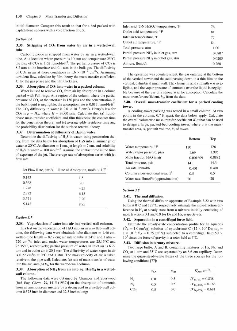
C03 09/29/2010 Page 138
initial diameter. Compare this result to that for a bed packed with
naphthalene spheres with a void fraction of 0.5.
Section 3.6
3.35. Stripping of CO2 from water by air in a wetted-wall
tube.
Carbon dioxide is stripped from water by air in a wetted-wall
tube. At a location where pressure is 10 atm and temperature 25�C,the flux of CO2 is 1.62 lbmol/h-ft2. The partial pressure of CO2 is
8.2 atm at the interface and 0.1 atm in the bulk gas. The diffusivity
of CO2 in air at these conditions is 1.6 � 10�2 cm2/s. Assuming
turbulent flow, calculate by film theory the mass-transfer coefficient
kc for the gas phase and the film thickness.
3.36. Absorption of CO2 into water in a packed column.
Water is used to remove CO2 from air by absorption in a column
packed with Pall rings. At a region of the column where the partial
pressure of CO2 at the interface is 150 psia and the concentration in
the bulk liquid is negligible, the absorption rate is 0.017 lbmol/h-ft2.
The CO2 diffusivity in water is 2.0 � 10�5 cm2/s. Henry’s law for
CO2 is p ¼ Hx, where H ¼ 9,000 psia. Calculate the: (a) liquid-
phase mass-transfer coefficient and film thickness; (b) contact time
for the penetration theory; and (c) average eddy residence time and
the probability distribution for the surface-renewal theory.
3.37. Determination of diffusivity of H2S in water.
Determine the diffusivity of H2S in water, using penetration the-
ory, from the data below for absorption of H2S into a laminar jet of
water at 20�C. Jet diameter ¼ 1 cm, jet length¼ 7 cm, and solubility
of H2S in water ¼ 100 mol/m3. Assume the contact time is the time
of exposure of the jet. The average rate of absorption varies with jet
flow rate:
Jet Flow Rate, cm3/s Rate of Absorption, mol/s � 106
0.143 1.5
0.568 3.0
1.278 4.25
2.372 6.15
3.571 7.20
5.142 8.75
Section 3.7
3.38. Vaporization of water into air in a wetted-wall column.
In a test on the vaporization of H2O into air in a wetted-wall col-
umn, the following data were obtained: tube diameter ¼ 1.46 cm;
wetted-tube length ¼ 82.7 cm; air rate to tube at 24�C and 1 atm ¼720 cm3/s; inlet and outlet water temperatures are 25.15�C and
25.35�C, respectively; partial pressure of water in inlet air is 6.27
torr and in outlet air is 20.1 torr. The diffusivity of water vapor in air
is 0.22 cm2/s at 0�C and 1 atm. The mass velocity of air is taken
relative to the pipe wall. Calculate: (a) rate of mass transfer of water
into the air; and (b) KG for the wetted-wall column.
3.39. Absorption of NH3 from air into aq. H2SO4 in a wetted-
wall column.
The following data were obtained by Chamber and Sherwood
[Ind. Eng. Chem., 29, 1415 (1937)] on the absorption of ammonia
from an ammonia-air mixture by a strong acid in a wetted-wall col-
umn 0.575 inch in diameter and 32.5 inches long:
Inlet acid (2-N H2SO4) temperature, �F 76
Outlet acid temperature, �F 81
Inlet air temperature, �F 77
Outlet air temperature, �F 84
Total pressure, atm 1.00
Partial pressure NH3 in inlet gas, atm 0.0807
Partial pressure NH3 in outlet gas, atm 0.0205
Air rate, lbmol/h 0.260
The operation was countercurrent, the gas entering at the bottom
of the vertical tower and the acid passing down in a thin film on the
vertical, cylindrical inner wall. The change in acid strength was neg-
ligible, and the vapor pressure of ammonia over the liquid is negligi-
ble because of the use of a strong acid for absorption. Calculate the
mass-transfer coefficient, kp, from the data.
3.40. Overall mass-transfer coefficient for a packed cooling
tower.
A cooling-tower packing was tested in a small column. At two
points in the column, 0.7 ft apart, the data below apply. Calculate
the overall volumetric mass-transfer coefficient Kya that can be used
to design a large, packed-bed cooling tower, where a is the mass-
transfer area, A, per unit volume, V, of tower.
Bottom Top
Water temperature, �F 120 126
Water vapor pressure, psia 1.69 1.995
Mole fraction H2O in air 0.001609 0.0882
Total pressure, psia 14.1 14.3
Air rate, lbmol/h 0.401 0.401
Column cross-sectional area, ft2 0.5 0.5
Water rate, lbmol/h (approximation) 20 20
Section 3.8
3.41. Thermal diffusion.
Using the thermal diffusion apparatus of Example 3.22 with two
bulbs at 0�C and 123�C, respectively, estimate the mole-fraction dif-
ference in H2 at steady state from a mixture initially consisting of
mole fractions 0.1 and 0.9 for D2 and H2, respectively.
3.42. Separation in a centrifugal force field.
Estimate the steady-state concentration profile for an aqueous
ðV̂B ¼ 1:0 cm3/gÞ solution of cytochrome C ð12� 103 Da; xA0¼
1� 10�6; V̂A ¼ 0:75 cm3/gÞ subjected to a centrifugal field 50 �103 times the force of gravity in a rotor held at 4�C.3.43. Diffusion in ternary mixture.
Two large bulbs, A and B, containing mixtures of H2, N2, and
CO2 at 1 atm and 35�C are separated by an 8.6-cm capillary. Deter-
mine the quasi-steady-state fluxes of the three species for the fol-
lowing conditions [77]:
xi,A xi,B D0AB, cm2/s
H2 0.0 0.5 D’H2-N2¼ 0.838
N2 0.5 0.5 D’H2-CO2¼ 0.168
CO2 0.5 0.0 D’N2-CO2¼ 0.681
138 Chapter 3 Mass Transfer and Diffusion