arX

iv:1

209.

1322

v1 [

cs.C

R]

6 S

ep 2

012

Differentially Private Grids for Geospatial DataWahbeh Qardaji, Weining Yang, Ninghui Li

Department of Computer Science, Purdue University305 N. University Street, West Lafayette, IN 47907, USA{wqardaji, yang469, ninghui}@cs.purdue.edu

Abstract— In this paper, we tackle the problem of constructinga differentially private synopsis for two-dimensional datasets suchas geospatial datasets. The current state-of-the-art methods workby performing recursive binary partitioning of the data dom ains,and constructing a hierarchy of partitions. We show that thekeychallenge in partition-based synopsis methods lies in choosing theright partition granularity to balance the noise error and t he non-uniformity error. We study the uniform-grid approach, whic happlies an equi-width grid of a certain size over the data domainand then issues independent count queries on the grid cells.Thismethod has received no attention in the literature, probably dueto the fact that no good method for choosing a grid size wasknown. Based on an analysis of the two kinds of errors, wepropose a method for choosing the grid size. Experimental resultsvalidate our method, and show that this approach performs aswell as, and often times better than, the state-of-the-art methods.

We further introduce a novel adaptive-grid method. Theadaptive grid method lays a coarse-grained grid over the dataset,and then further partitions each cell according to its noisycount. Both levels of partitions are then used in answeringqueries over the dataset. This method exploits the need to havefiner granularity partitioning over dense regions and, at thesame time, coarse partitioning over sparse regions. Throughextensive experiments on real-world datasets, we show thatthisapproach consistently and significantly outperforms the uniform-grid method and other state-of-the-art methods.

I. I NTRODUCTION

We interact with location-aware devices on a daily basis.Such devices range from GPS-enabled cell-phones and tablets,to navigation systems. Each device can report a multitude oflocation data to centralized servers. Such location information,commonly referred to as geospatial data, can have tremen-dous benefits if properly processed and analyzed. For manybusinesses, a location-based view of information can enhancebusiness intelligence and enable smarter decision making.Formany researchers, geospatial data can add an interesting di-mension. Location information from cell-phones, for instance,can help in various social research that is interested in howpopulations settle and congregate. Furthermore, locationfromin-car navigation systems can help provide information onareas of common traffic congestion.

If shared, such geo-spatial data can have significant im-pact for research and other uses. Sharing such information,however, can have significant privacy implications. In thispaper, we study the problem of releasing static geo-spatialdata in a private manner. In particular, we introduce methodsof releasing a synopsis of two-dimensional datasets whilesatisfying differential privacy.

Differential privacy [1] has recently become the defactostandard for privacy preserving data release, as it is capableof providing strong worst-case privacy guarantees. We con-sider two-dimensional, differentially private, synopsismethodsin the following framework. Given a dataset and the two-dimensional domain that tuples in the dataset are in, weview each tuple as a point in two-dimensional space. Onepartitions the domain into cells, and then obtains noisy countsfor each cell in a way that satisfies differential privacy. Thedifferentially private synopsis consists of the boundaries ofthese cells and their noisy counts. This synopsis can then beused either for generating a synthetic dataset, or for answeringqueries directly.

In general, when answering queries, there are two sourcesof error in such differentially private synopsis methods. Thefirst source is the noise added to satisfy differential privacy.This noise has a predefined variance and is independent of thedataset, but depends on how many cells are used to answera query. The second source is the nature of the dataset itself.When we issue a query which only partially intersects withsome cell, then we would have to estimate how many datapoints are in the intersected cells, assuming that the data pointsare distributed uniformly. The magnitude of this error dependsboth on the distribution of points in the dataset and on thepartitioning. Our approach stems from careful examinationofhow these two sources of error depend on the grid size.

Several recent papers have attempted to develop suchdifferentially private synopsis methods for two-dimensionaldatasets [2], [3]. These papers adapt spatial indexing methodssuch as quadtrees and kd-trees to provide a private descriptionof the data distribution. These approaches can all be viewedas adapting the binary hierarchical method, which works wellfor 1-dimensional datasets, to the case of 2 dimensions. Theemphasis is on how to perform the partitioning, and the resultis a deep tree.

Somewhat surprisingly, none of the existing papers on sum-marizing multi-dimensional datasets compare with the simpleuniform-grid method, which applies an equi-widthm × mgrid over the data domain and then issues independent countqueries on the grid cells. We believe one reason is that theaccuracy ofUG is highly dependent on the grid sizem, andhow to choose the best grid size was not known. We propose

choosingm to be√

Nǫc , whereN is the number of data points,

ǫ is the total privacy budget, andc is some small constantdepending on the dataset. Extensive experimental results,using

4 real-world datasets of different sizes and features, validateour method of choosingm. Experimental results also suggestthat settingc = 10 work well for datasets of different sizesand different choices ofǫ, and show thatUG performs as wellas, and often times better than the state-of-the-art hierarchicalmethods in [2], [3].

This result is somewhat surprising, as hierarchical methodshave been shown to greatly outperform the equivalence ofuniform-grid in 1-dimensional case [4], [5]. We thus analyzethe effect of dimensionality on the effectiveness of usinghierarchies.

We further introduce a novel adaptive-grid method. Thismethod is motivated by the need to have finer granularitypartitioning over dense regions and, at the same time, coarsepartitioning over sparse regions. The adaptive grid methodlays a coarse-grained grid over the dataset, and then furtherpartitions each cell according to its noisy count. Both levelsof partitions are then used in answering queries over thedataset. We propose methods to choose the parameters forthe partitioning by careful analysis of the aforementionedsources of error. Extensive experiments validate our methodsfor choosing the parameters, and show that the adaptive-gridmethod consistently and significantly outperforms the uniformgrid method and other state-of-the-art methods.

The contributions of this paper are as follows:1) We identify that the key challenge in differentially

private synopsis of geospatial datasets is how to choosethe partition granularity to balance errors due to twosources, and propose a method for choosing grid sizefor the uniform grid method, based on an analysis ofhow the errors depend on the grid size.

2) We propose a novel, simple, and effective adaptive gridmethod, together with methods for choosing the keyparameters.

3) We conducted extensive evaluations using 4 datasets ofdifferent sizes, including geo-spatial datasets that havenot been used in differentially private data publishingliterature before. Experimental results validate our meth-ods and show that they outperform existing approaches.

4) We analyze why hierarchical methods do not performwell in 2-dimensional case, and predict that they wouldperform even worse with higher dimensions.

The rest of this paper is organized as follows. In Section II,we set the scope of the paper by formally defining the prob-lem of publishing two dimensional datasets using differentialprivacy. In Section III, we discuss previous approaches andrelated work. We present our approach in Section IV, andpresent the experimental results supporting our claims inSection V. Finally, we conclude in Section VI.

II. PROBLEM DEFINITION

A. Differential Privacy

Informally, differential privacy requires that the outputof adata analysis mechanism be approximately the same, even ifany single tuple in the input database is arbitrarily added orremoved.

Definition 1 (ǫ-Differential Privacy [1], [6]): Arandomized mechanismA gives ǫ-differential privacy iffor any pair of neighboring datasetsD and D′, and anyS ∈ Range(A),

Pr [A(D) = S] ≤ eǫ · Pr [A(D′) = S] .In this paper we consider two datasetsD and D′ to be

neighbors if and only if eitherD = D′ + t or D′ = D + t,whereD+t denotes the dataset resulted from adding the tuplet to the datasetD. We useD ≃ D′ to denote this. This protectsthe privacy of any single tuple, because adding or removingany single tuple results ineǫ-multiplicative-bounded changesin the probability distribution of the output. If any adversarycan make certain inference about a tuple based on the output,then the same inference is also likely to occur even if the tupledoes not appear in the dataset.

Differential privacy is composable in the sense that combin-ing multiple mechanisms that satisfy differential privacyforǫ1, · · · , ǫm results in a mechanism that satisfiesǫ-differentialprivacy for ǫ =

∑

i ǫi. Because of this, we refer toǫ asthe privacy budget of a privacy-preserving data analysis task.When a task involves multiple steps, each step uses a portionof ǫ so that the sum of these portions is no more thanǫ.

To compute a functiong on the datasetD in a differentiallyprivately way, one can add tog(D) a random noise drawn fromthe Laplace distribution. The magnitude of the noise dependson GSg, theglobal sensitivityor theL1 sensitivity ofg. Sucha mechanismAg is given below:

Ag(D) = g(D) + Lap(

GSg

ǫ

)

where GSg = max(D,D′):D≃D′ |g(D)− g(D′)|,and Pr [Lap (β) = x] = 1

2β e−|x|/β

In the above,Lap (β) denotes a random variable sampled fromthe Laplace distribution with scale parameterβ. The varianceof Lap (β) is 2β2; hence the standard deviation ofLap

(

GSg

ǫ

)

is√2GSg

ǫ .

B. Problem Definition

We consider the following problem. Given a 2-dimensionalgeospatial datasetD, our aim is to publish a synopsis of thedataset to accurately answer count queries over the dataset.We consider synopsis methods in the following framework.Given a dataset and the two-dimensional domain that tuplesin the dataset are in, we view each tuple as a point in two-dimensional space. One partitions the domain into cells, andthen obtains noisy counts for each cell in a way that satisfiesdifferential privacy. The differentially private synopsis consistsof the boundary of these cells and their noisy counts. Thissynopsis can then be used either for generating a syntheticdataset, or for answering queries directly.

We assume that each query specifies a rectangle in thedomain, and asks for the number of data points that fall inthe rectangle. Such a count query can be answered using thenoisy counts for cells in the following fashion. If a cell iscompletely included in the query rectangle, then the noisy

count is included in the total. If a cell is partially included, thenone estimates the point count in the intersection between thecell and the query rectangle, assuming that the points withinthe cell is distributed uniformly. For instance, if only half ofthe area of the cell is included in the query, then one assumesthat half of the points are covered by the query.

Two Sources of Error. Under this method, there are twosources of errors when answering a query. Thenoise error isdue to the fact that the counts are noisy. To satisfy differentialprivacy, one adds, to each cell, an independently generatednoise, and these noises have the same standard deviation,which we useσ to denote. When summing up the noisy countsof q cells to answer a query, the resulting noise error is the sumof the corresponding noises. As these noises are independentlygenerated zero-mean random variables, they cancel each otherout to a certain degree. In fact, because these noises areindependently generated, the variance of their sum equals thesum of their variances. Therefore, the sum has varianceqσ2,corresponding to a standard deviation of

√qσ. That is, the

noise error of a query grows linearly in√q. Therefore, the

finer granularity one partitions the domain into, the more cellsare included in a query, and the larger the noise error is.

The second source of error is caused by cells that intersectwith the query rectangle, but are not contained in it. For thesecells, we need to estimate how many data points are in theintersected cells assuming that the data points are distributeduniformly. This estimation will have errors when the datapoints are not distributed uniformly. We call this thenon-uniformity error . The magnitude of the non-uniformity errorin any intersected cell, in general, depends on the number ofdata points in that cell, and is bounded by it. Therefore, thefiner the partition granularity, the lower the non-uniformityerror.

As argued above, reducing the noise error and non-uniformity error imposes conflicting demands on the partitiongranularity. The main challenge of partition-based differen-tially private synopsis lies in how to meet this challengeand reconcile the conflicting needs of noise error and non-uniformity error.

III. PREVIOUS APPROACHES ANDRELATED WORK

Differential privacy was presented in a series of papers [7],[8], [9], [6], [1] and methods of satisfying it for evaluatingsome function over the dataset are presented in [1], [10], [11].

Recursive Partitioning. Most approaches that directly ad-dress two-dimensional and spatial datasets use recursive par-titioning [12], [3], [2]. These approaches perform a recursivebinary partitioning of the data domain.

Xiao et al. [2] proposed adapting the standard spatial index-ing method, KD-trees, to provide differential privacy. Nodesin a KD-tree are recursively split along some dimension. Inorder to minimize the non-uniformity error, Xiao et al. use theheuristic to choose the split point such that the two sub-regionsare as close to uniform as possible.

Cormode et al. [3] proposed a similar approach. Instead ofusing a uniformity heuristic, they split the nodes along the

median of the partition dimension. The height of the tree ispredetermined and the privacy budget is divided among thelevels. Part of the privacy budget is used to choose the median,and part is used to obtain the noisy count. [3] also proposedcombining quad-trees with noisy median-based partitioning.In the quadtree, nodes are recursively divided into four equalregions via horizontal and vertical lines through the midpointof each range. Thus no privacy budget is needed to choosethe partition point. The method that gives the best performancein [3] is a hybrid approach, which they call “KD-hybrid”. Thismethod uses a quadtree for the first few levels of partitions,and then uses the KD-tree approach for the other levels.A number of other optimizations were also applied in KD-hybrid, including the constrained inference presented in [4],and optimized allocation of privacy budget. Their experimentsindicate that “KD-hybrid” outperforms the KD-tree basedapproach and the approach in [2].

Qardaji and Li [12] proposed a general recursive partitioningframework for multidimensional datasets. At each level ofrecursion, partitioning is performed along the dimension whichresults in the most balanced partitioning of the data points. Thebalanced partitioning employed by this method has the effectof producing regions of similar size. When applied to two-dimensional datasets, this approach is very similar to buildinga KD-tree based on noisy median.

We experimentally compare with the state-of-the-art KD-hybrid method. In Section IV-C, we analyze the effect ofdimensionality and show that hierarchical methods providelimited benefit in the2-dimensional case.

Hierarchical Transformations. The recursive partitioningmethods above essentially build a hierarchy over a representa-tion of the data points. Several approaches have been presentedin the literature to improve count queries over such hierarchies.

In [4], Hay et al. proposed the notion of constrained infer-ence for hierarchical methods to improve accuracy for rangequeries. This work has been mostly developed in the contextof one-dimensional datasets. Using this approach, one wouldarrange all queried intervals into a binary tree, where the unit-length intervals are the leaves. Count queries are then issuedat all the nodes in the tree. Constrained inference exploitstheconsistency requirement that the parent’s count should equalthe sum of all children’s counts to improve accuracy.

In [5], Xiao et al. propose the Privlet method answering his-togram queries, which uses wavelet transforms. Their approachapplies a Harr wavelet transform to the frequency matrix ofthe dataset. A Harr wavelet essentially builds a binary treeover the dataset, where each node (or “coefficient”) representsthe difference between the average value of the nodes in itsright subtree, and the average value of the nodes in its leftsubtree. The privacy budget is divided among the differentlevels, and the method then adds noise to each transformationcoefficient proportional to its sensitivity. These coefficients arethen used to regenerate an anonymized version of the datasetby applying the reverse wavelet transformation. The benefitof using wavelet transforms is that they introduce a desirable

noise canceling effect when answering range queries.For two dimensional datasets, this method uses standard

decomposition when applying the wavelet transform. Viewingthe dataset as a frequency matrix, the method first applies theHarr wavelet transform on each row. The result is a vector ofdetail coefficients for each row. Then, using the matrix of detailcoefficients as input, the method applies the transformation onthe columns. Noise is then added to each cell, proportional tothe sensitivity of the coefficient in that cell. To reconstructthe noisy frequency matrix, the method applies the reversetransformation on each column and then each row.

Both constrained inference and wavelet methods have beenshown to be very effective at improving query accuracy inthe 1-dimensional case. Our experiments show that applyingthem to a uniform grid provides small improvements for the2-dimensional datasets. We note that these methods can onlybe applied when one has decided what are the leaf cells.When combined with the uniform grid method, it requires amethod to choose the right grid size, as the performance willbe poor when a wrong grid size is used. In Section V, weexperimentally compare with the wavelet method.

Other related work. Blum et al. [13] proposed an approachthat employs non-recursive partitioning, but their results aremostly theoretical and lack general practical applicability tothe domain we are considering.

[14], [15], [16] provide methods of differentially privaterelease which assume that the queries are known before publi-cation. The most recent of such works by Li and Miklau [16]proposes the matrix mechanism. Given a workload of countqueries, the mechanism automatically selects a different set ofstrategy queries to answer privately. It then uses those answersto derive answers to the original workload. Other techniquesfor analyzing general query workloads under differential pri-vacy have been discussed in [17], [18]. These approaches alsorequire the base cells to be fixed. Furthermore, they requiretheexistence of a known set of queries, which are represented asamatrix, and then compute how to combine base cells to answerthe original queries. It is unclear how to use this method whenone aims at answering arbitrary range queries.

A number of approaches exist for differentially privateinteractive data analysis, e.g., [19], and methods of improvingthe accuracy of such release [20] have been suggested. In suchworks, however, one interacts with a privacy aware databaseinterface rather than getting access to a synopsis of the dataset.Our approach deals with the latter.

IV. T HE ADAPTIVE PARTITIONING APPROACH

In this section, we present our proposed methods.

A. The Uniform Grid Method -UG

Perhaps the simplest method one can think of is the UniformGrid (UG) method. This approach partitions the data domaininto m × m grid cells of equal size, and then obtains anoisy count for each cell. Somewhat surprisingly, none ofthe existing papers on summarizing multi-dimensional datasetscompare withUG. We believe one reason is that the accuracy

of UG is highly dependent on the grid sizem, and how tochoose the best grid size was not known.

We propose the following guideline for choosingm in orderto minimize the sum of the two kinds of errors presented inSection II.

Guideline 1: In order to minimize the errors due toǫ-DPUG, the grid size should be about

√

Nǫ

c,

whereN is the number of data points,ǫ is the total privacybudget, andc is some small constant depending on the dataset.Our experimental results suggest that settingc = 10 workswell for the datasets we have experimented with.

Below we present our analysis supporting this guideline.As the sensitivity of the count query is1, the noise added foreach cell follows the distributionLap

(

1ǫ

)

and has a standard

deviation of√2ǫ . Given anm×m grid, and a query that selects

r portion of the domain (wherer is the ratio of the area ofthe query rectangle to the area of the whole domain), aboutrm2 cells are included in the query, and the total noise errorthus has standard deviation of

√2rm2

ǫ =√2rmǫ .

The non-uniformity error is proportional to the number ofdata points in the cells that fall on the border of the queryrectangle. For a query that selectsr portion of the domain,it has four edges, whose lengths are proportional to

√r of

the domain length; thus the query’s border contains on theorder of

√rm cells, which on average includes on the order

of√rm × N

m2 =√rNm data points. Assuming that the non-

uniformity error on average is some portion of the total densityof the cells on the query border, then the non-uniformity erroris

√rN

c0mfor some constantc0.

To minimize the two errors’ sum,√2rmǫ +

√rN

mc0, we should

setm to√

Nǫc , wherec =

√2c0.

Using Guideline 1 requires knowingN , the number of datapoints. Obtaining a noisy estimate ofN using a very smallportion of the total privacy budget suffices.

The parameterc depends on the uniformity of the dataset.In the extreme case where the dataset is completely uniform,then the optimal grid size is1×1. That is, the best method is toobtain as accurate a total count as possible, and then any querycan be fairly accurately answered by computing what fractionof the region is covered by the query. This corresponds to alargec. When a dataset is highly non-uniform, then a smallercvalue is desirable. In our experiments, we observe that settingc = 10 gives good results across datasets of different kinds.

B. The Adaptive Grids Approach -AG

The main disadvantage ofUG is that it treats all regionsin the dataset equally. That is, both dense and sparse regionsare partitioned in exactly the same way. This is not optimal.If a region has very few points, this method might result inover-partitioning of the region, creating a set of cells withclose to zero data points. This has the effect of increasing thenoise error with little reduction in the non-uniformity error. On

the other hand, if a region is very dense, this method mightresult inunder-partitioning of the region. As a result, the non-uniformity error would be quite large.

Ideally, when a region is dense, we want to use finergranularity partitioning, because the non-uniformity error inthis region greatly outweighs that of noise error. Similarly,when a region is sparse (having few data points), we want touse a more coarse grid there. Based on this observation, wepropose an Adaptive Grids (AG) approach.

The AG approach works as follows. We first lay a coarsem1×m1 grid over the data domain, creating(m1)

2 first-levelcells, and then we issue a count query for each cell using aprivacy budgetαǫ, where0 < α < 1. For each cell, letN ′ bethe noisy count of the cell,AG then partitions the cell using agrid size that is adaptively chosen based onN ′, creating leafcells. The parameterα determines how to split the privacybudget between the two levels.

Applying Constrained Inference. As discussed in Sec-tion III, constrained inference has been developed in thecontext of one-dimensional histograms to improve hierarchicalmethods [4]. TheAG method produces a 2-level hierarchy. Foreach first-level cell, if it is further partitioned into am2 ×m2

grid, we can perform constrained inference.Let v be the noisy count of a first-level cell, and let

u1,1, . . . , um2,m2be the noisy counts of the cells thatv is

further partitioned into in the second level. One can then applyconstrained inference as follows. First, one obtains a moreaccurate countv′ by taking the weighted average ofv and thesum ofui,j such that the standard deviation of the noise errorat v′ is minimized.

v′ =α2m2

2

(1− α)2 + α2m22

v +(1 − α)2

(1 − α)2 + α2m22

∑

ui,j

This value is then propagated to the leaf nodes by distribut-ing the difference among all nodes equally

u′i,j = ui,j +

(

v′ −∑

ui,j

)

.

Whenm2 = 1, the constrained inference step becomes issuinganother query with budget(1 − α)ǫ and then computing aweighted average of the two noisy counts.

Choosing Parameters forAG. For theAG method, we needto decide the formula to adaptively determine the grid size foreach first-level cell. We propose the following guideline.

Guideline 2: Given a cell with a noisy count ofN ′, tominimize the errors, this cell should be partitioned intom2 ×m2 cells, wherem2 is computed as follows:

√

N ′(1 − α)ǫ

c2

,

where(1− α)ǫ is the remaining privacy budget for obtainingnoisy counts for leaf cells,c2 = c/2, andc is the same constantas in Guideline 1.

The analysis to support this guideline is as follows. Whenthe first-level cell is further partitioned intom2 × m2 leaf

cells, only queries whose borders go through this first-levelcell will be affected. These queries may include0, 1, 2,· · · , up to m2 − 1 rows (or columns) of leaf cells, and thus0,m2, 2m2, · · · , (m2−1)m2 leaf cells. When a query includesmore than half of these leaf cells, constrained inference has theeffect that the query is answered using the count obtained inthe first level cell minus those leaf cells that are not includedin the query. Therefore, on average a query is answered using

1

m2

(

m2−1∑

i=0

min(i,m2 − i)

)

m2 ≈ (m2)2

4

leaf cells, and the average noise error is on the order of√

(m2)2

4

√2

(1−α)ǫ . The average non-uniformity error is aboutN ′

c0m2

; thereby to minimize their sum, we should choosem2

to be about√

N ′(1−α)ǫ√2c0/2

.The choice ofm1, the grid-size for the first level, is less

critical than the choice ofm2. Whenm1 is larger, the averagedensity of each cell is smaller, and the further partitioning stepwill partition each cell into fewer number of cells. Whenm1

is smaller, the further partitioning step will partition each cellinto more cells. In general,m1 should be less than the gridsize forUG computed according to Guideline 1, since it willfurther partition each cell. At the same time,m1 should notbe too small either. We set

m1 = max

(

10,1

4

⌈

√

Nǫ

c

⌉)

.

The choice ofα also appears to be less critical. Ourexperiments suggest that settingα to be in the range of[0.2, 0.6] results in similar accuracy. We setα = 0.5.

C. Comparing with Existing Approaches

We now compare our proposedUG andAG with existinghierarchical methods, in terms of runtime efficiency, simplicity,and extensibility to higher dimensional datasets.

Efficiency. TheUG andAG methods are conceptually simpleand easy to implement. They also work well with very largedatasets that cannot fit into memory.UG can be performed bya single scan of the data points. For each data point,UG justneeds to increase the counter of the cell that the data point isin by 1.AG requires two passes over the dataset. The first passis similar to that ofUG. In the second pass, it first computeswhich first-level cell the data point is in, and then which leafcell it is in. It then increases the corresponding counter.

We point out that another major benefit ofUG andAG overrecursive partition-based methods are their higher efficiency.For all these methods, the running time is linear in the depthof the tree, as each level of the tree requires one pass overthe dataset. Existing recursive partitioning methods havemuchdeeper trees (e.g., reaching 16 levels is common for 1 milliondata points). Furthermore, these methods require expensivecomputation to choose the partition points.

Effect of Dimensionality. Existing recursive partitioningapproaches can be viewed as adapting the binary hierarchical

method, which works well for 1-dimensional dataset, to thecases of 2 dimensions. Some of these methods adapt quadtreemethods, which can be viewed as extending 1-dimensionalbinary trees to 2 dimensions. The emphasis is on how to per-form the binary partition, e.g., using noisy mean, exponentialmethod for finding the median, exponential method using non-uniformity measurement, etc. The result is a deep tree.

We observe, however, while a binary hierarchical tree workswell for the 1-dimensional case, their benefit for the 2-dimensional case is quite limited, and the benefit can only de-crease with higher dimensionality. When building a hierarchy,the interior of a query can be answered by higher-level nodes,but the borders of the query have to be answered using leafnodes. The higher the dimensionality, the larger the portion ofthe border region.

For example, for a 1-dimensional dataset with domaindivided intoM cells, when one groups eachb adjacent cellsinto one larger cell, each larger cell is of sizebM of the wholedomain. Each query has2 border regions which need to beanswered by leaf cells; each region is of size on the order ofthat of one larger cell, i.e.,bM of the whole domain. In the 2-dimensional case, with am×m grid and a total ofM = m×mcells, if one groupsb =

√b×

√b adjacent cells together, then

a query’s border, which needs to be answered by leaf nodes,has4 sides, and each side is of size on the order of

√b√M

of

the whole domain. Note that4√b√M

is much larger than2 bM ,

sinceM is always much larger thanb. For example, whenM = 10, 000 andb = 4, 4

√b√M

= 0.08, and2 bM = 0.0008.

Therefore, in 2-dimensional case, one benefits much lessfrom a hierarchy, which provides less accurate counts for theleaf cells. This effect keeps growing with dimensionality.Ford dimensions, the border of a query has2d hyperplanes, eachof size on the order of

d√b

d√M

. In our experiments, we haveobserved some small benefits for using hierarchies, which weconjecture will disappear with3 or higher dimensional cases.

This analysis suggests that our approach of starting from theUniform Grid method and trying to improve upon this methodis more promising than trying to improve a hierarchical treebased method. When focusing on Uniform Grid, the emphasisin designing the algorithm shifts from choosing the axis forpartitioning to choosing the partition granularity. When onepartitions a cell into two sub-cells, the question of how toperform the partitioning depending on the data in the cellseems important and may affect the performance; and thusone may want to use part of the privacy budget to figureout what the best partitioning point is. On the other hand,when one needs to partition a cell into, e.g.,8 × 8, sub-cells in a differentially private way, it appears that the onlyfeasible solution is to do equi-width partition. Hence the onlyparameter of interest is what is the grid size.

V. EXPERIMENTAL RESULTS

A. Methodology

We have conducted extensive experiments using four realdatasets, to compare the accuracy of different methods and to

validate our analysis of the choice of parameters.

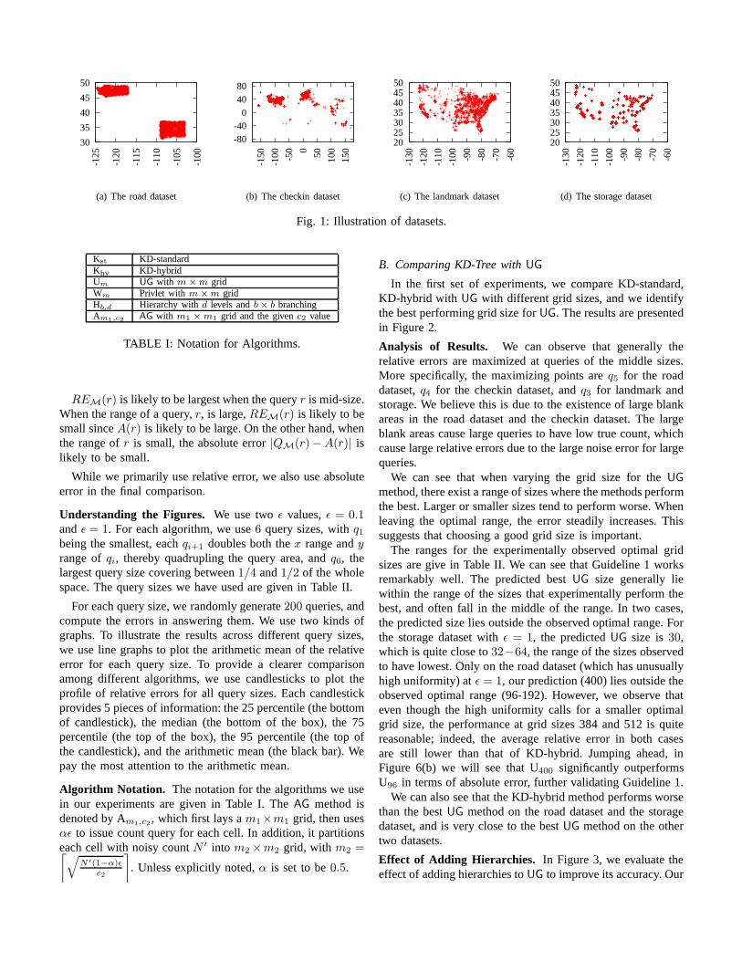
Datasets. We illustrate these datasets by plotting the datapoints directly in Figure 1. We also present the parameters forthese datasets in Table II.

The first dataset (which we call the “road” dataset) includesthe GPS coordinates of road intersections in the states ofWashington and New Mexico, obtained from 2006 TIGER/-Line from US Census. This is the dataset that was used in[3] for experimental evaluations. There are about 1.6M datapoints. As illustrated in Figure 1(a), the distribution of the datapoints is quite unusual. There are large blank areas with twodense regions (corresponding to the two states).

The second dataset is derived from the checkin dataset1

from the Gowalla location-based social networking website,where users share their locations by checking-in. This datasetrecords time and location information of check-ins made byusers over the period of Feb. 2009 - Oct. 2010. We onlyuse the location information. There are about 6.4M datapoints. The large size of the dataset makes it infeasible torun the implementation of KD-tree based methods obtainedfrom authors of [3] due to memory constraints. We thussampled 1M data points from this dataset, and we call thisthe “checkin” dataset. As illustrated in Figure 1(b), the shapevaguely resembles a world map, but with the more developedand/or populous areas better represented than other areas.

We obtained both the third dataset (“landmark” dataset)and the fourth dataset (“storage” datset) from infochimps.The landmark dataset2 consists of locations of landmarksin the 48 continental states in the United State. The listedlandmarks range from schools and post offices to shoppingcenters, correctional facilities, and train stations fromthe 2010Census TIGER point landmarks. There are over 870k datapoints. As illustrated in Figure 1(b), the dataset appears tomatch the population distribution in US.

The storage dataset3 includes US storage facility locations.Included are national chain storage facilities, as well as locallyowned and operated facilities. This is a small dataset, consist-ing about 9000 data points. We chose to use this dataset toanalyze whether our analysis and guideline in Section IV holdsfor both large and small datasets.

Absolute and Relative Error. Following [3], we primarilyconsider the relative error, defined as follows: For a queryr,we useA(r) to denote the correct answer tor. For a methodM and a queryr, we useQM(r) to denote the answer to thequeryr when using the histogram constructed by methodMto answer the queryr, then the relative error is defined as

REM(r) =|QM(r)−A(r)|max{A(r), ρ}

where we setρ to be0.001∗ |D|, whereD is the total numberof data points inD. This avoids dividing by 0 whenA(r) = 0.

1http://snap.stanford.edu/data/loc-gowalla.html2http://www.infochimps.com/datasets/storage-facilities-by-landmarks3http://www.infochimps.com/datasets/storage-facilities-by-neighborhood–2

30

35

40

45

50-1

25

-120

-115

-110

-105

-100

(a) The road dataset

-80-40

0 40 80

-150

-100 -50 0 50

100

150

(b) The checkin dataset

20 25 30 35 40 45 50

-130

-120

-110

-100 -90

-80

-70

-60

(c) The landmark dataset

20 25 30 35 40 45 50

-130

-120

-110

-100 -90

-80

-70

-60

(d) The storage dataset

Fig. 1: Illustration of datasets.

Kst KD-standardKhy KD-hybridUm UG with m×m gridWm Privlet with m×m gridHb,d Hierarchy withd levels andb× b branchingAm1,c2 AG with m1 ×m1 grid and the givenc2 value

TABLE I: Notation for Algorithms.

REM(r) is likely to be largest when the queryr is mid-size.When the range of a query,r, is large,REM(r) is likely to besmall sinceA(r) is likely to be large. On the other hand, whenthe range ofr is small, the absolute error|QM(r)−A(r)| islikely to be small.

While we primarily use relative error, we also use absoluteerror in the final comparison.

Understanding the Figures. We use twoǫ values,ǫ = 0.1andǫ = 1. For each algorithm, we use6 query sizes, withq1being the smallest, eachqi+1 doubles both thex range andyrange ofqi, thereby quadrupling the query area, andq6, thelargest query size covering between1/4 and1/2 of the wholespace. The query sizes we have used are given in Table II.

For each query size, we randomly generate200 queries, andcompute the errors in answering them. We use two kinds ofgraphs. To illustrate the results across different query sizes,we use line graphs to plot the arithmetic mean of the relativeerror for each query size. To provide a clearer comparisonamong different algorithms, we use candlesticks to plot theprofile of relative errors for all query sizes. Each candlestickprovides 5 pieces of information: the 25 percentile (the bottomof candlestick), the median (the bottom of the box), the 75percentile (the top of the box), the 95 percentile (the top ofthe candlestick), and the arithmetic mean (the black bar). Wepay the most attention to the arithmetic mean.

Algorithm Notation. The notation for the algorithms we usein our experiments are given in Table I. TheAG method isdenoted by Am1,c2 , which first lays am1×m1 grid, then usesαǫ to issue count query for each cell. In addition, it partitionseach cell with noisy countN ′ into m2 ×m2 grid, with m2 =⌈

√

N ′(1−α)ǫc2

⌉

. Unless explicitly noted,α is set to be0.5.

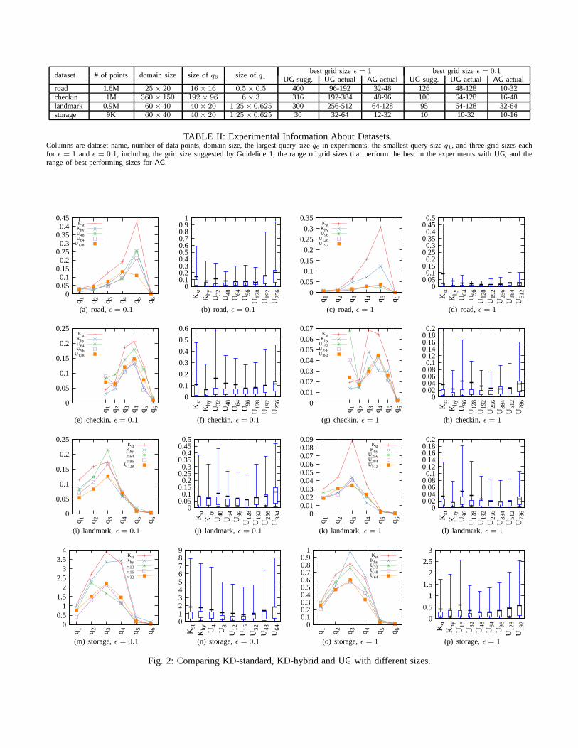
B. Comparing KD-Tree withUG

In the first set of experiments, we compare KD-standard,KD-hybrid with UG with different grid sizes, and we identifythe best performing grid size forUG. The results are presentedin Figure 2.

Analysis of Results. We can observe that generally therelative errors are maximized at queries of the middle sizes.More specifically, the maximizing points areq5 for the roaddataset,q4 for the checkin dataset, andq3 for landmark andstorage. We believe this is due to the existence of large blankareas in the road dataset and the checkin dataset. The largeblank areas cause large queries to have low true count, whichcause large relative errors due to the large noise error for largequeries.

We can see that when varying the grid size for theUG

method, there exist a range of sizes where the methods performthe best. Larger or smaller sizes tend to perform worse. Whenleaving the optimal range, the error steadily increases. Thissuggests that choosing a good grid size is important.

The ranges for the experimentally observed optimal gridsizes are give in Table II. We can see that Guideline 1 worksremarkably well. The predicted bestUG size generally liewithin the range of the sizes that experimentally perform thebest, and often fall in the middle of the range. In two cases,the predicted size lies outside the observed optimal range.Forthe storage dataset withǫ = 1, the predictedUG size is30,which is quite close to32−64, the range of the sizes observedto have lowest. Only on the road dataset (which has unusuallyhigh uniformity) atǫ = 1, our prediction (400) lies outside theobserved optimal range (96-192). However, we observe thateven though the high uniformity calls for a smaller optimalgrid size, the performance at grid sizes 384 and 512 is quitereasonable; indeed, the average relative error in both casesare still lower than that of KD-hybrid. Jumping ahead, inFigure 6(b) we will see that U400 significantly outperformsU96 in terms of absolute error, further validating Guideline 1.

We can also see that the KD-hybrid method performs worsethan the bestUG method on the road dataset and the storagedataset, and is very close to the bestUG method on the othertwo datasets.

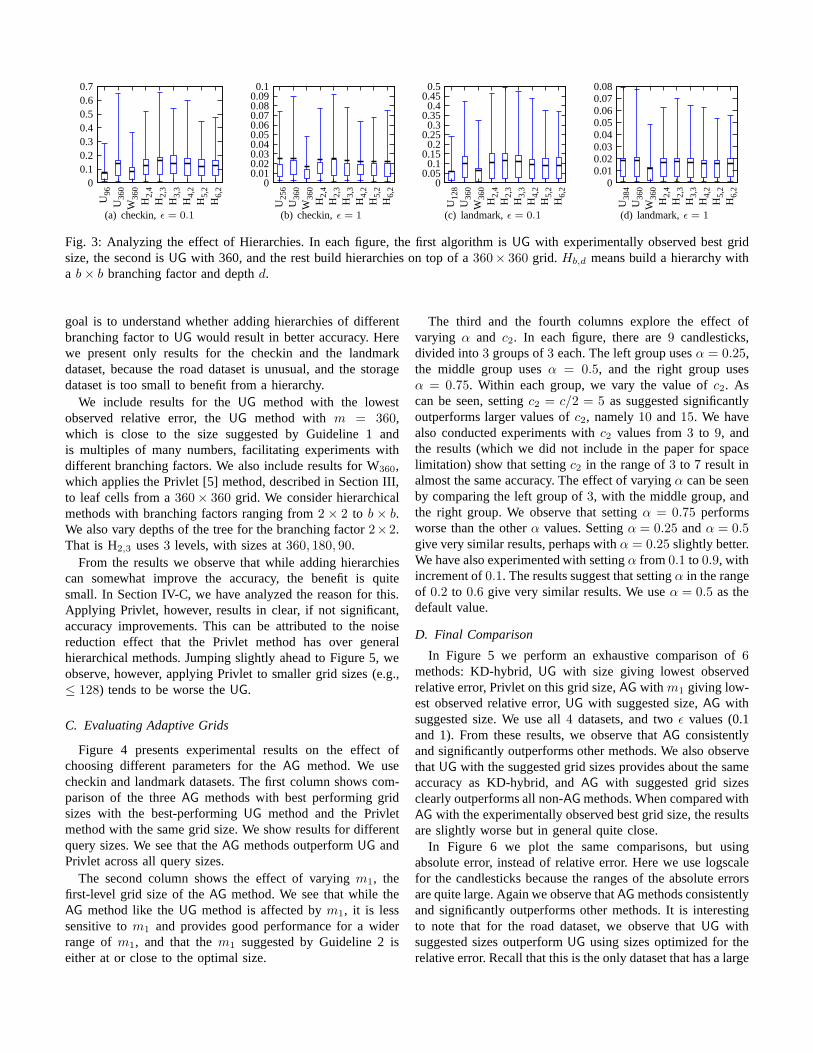
Effect of Adding Hierarchies. In Figure 3, we evaluate theeffect of adding hierarchies toUG to improve its accuracy. Our

dataset # of points domain size size ofq6 size ofq1best grid sizeǫ = 1 best grid sizeǫ = 0.1

UG sugg. UG actual AG actual UG sugg. UG actual AG actualroad 1.6M 25× 20 16× 16 0.5× 0.5 400 96-192 32-48 126 48-128 10-32checkin 1M 360 × 150 192 × 96 6× 3 316 192-384 48-96 100 64-128 16-48landmark 0.9M 60× 40 40× 20 1.25× 0.625 300 256-512 64-128 95 64-128 32-64storage 9K 60× 40 40× 20 1.25× 0.625 30 32-64 12-32 10 10-32 10-16

TABLE II: Experimental Information About Datasets.Columns are dataset name, number of data points, domain size, the largest query sizeq6 in experiments, the smallest query sizeq1, and three grid sizes eachfor ǫ = 1 and ǫ = 0.1, including the grid size suggested by Guideline 1, the rangeof grid sizes that perform the best in the experiments withUG, and therange of best-performing sizes forAG.

0 0.05 0.1

0.15 0.2

0.25 0.3

0.35 0.4

0.45

q 1 q 2 q 3 q 4 q 5 q 6

KstKhyU48U64

U128

(a) road,ǫ = 0.1

0 0.1 0.2 0.3 0.4 0.5 0.6 0.7 0.8 0.9

1

Kst

Khy

U32

U48

U64

U96

U12

8U

192

U25

6

(b) road,ǫ = 0.1

0

0.05

0.1

0.15

0.2

0.25

0.3

0.35

q 1 q 2 q 3 q 4 q 5 q 6

KstKhyU96

U128U192

(c) road,ǫ = 1

0 0.05 0.1

0.15 0.2

0.25 0.3

0.35 0.4

0.45 0.5

Kst

Khy

U64

U96

U12

8U

192

U25

6U

384

U51

2

(d) road,ǫ = 1

0

0.05

0.1

0.15

0.2

0.25

q 1 q 2 q 3 q 4 q 5 q 6

KstKhyU64U96

U128

(e) checkin,ǫ = 0.1

0

0.1

0.2

0.3

0.4

0.5

0.6

Kst

Khy

U32

U48

U64

U96

U12

8U

192

U25

6

(f) checkin, ǫ = 0.1

0

0.01

0.02

0.03

0.04

0.05

0.06

0.07

q 1 q 2 q 3 q 4 q 5 q 6

KstKhy

U192U256U384

(g) checkin,ǫ = 1

0 0.02 0.04 0.06 0.08 0.1

0.12 0.14 0.16 0.18 0.2

Kst

Khy

U96

U12

8U

192

U25

6U

384

U51

2U

786

(h) checkin,ǫ = 1

0

0.05

0.1

0.15

0.2

0.25

q 1 q 2 q 3 q 4 q 5 q 6

KstKhyU64U96

U128

(i) landmark,ǫ = 0.1

0 0.05 0.1

0.15 0.2

0.25 0.3

0.35 0.4

0.45 0.5

Kst

Khy

U48

U64

U96

U12

8U

192

U25

6U

384

(j) landmark,ǫ = 0.1

0 0.01 0.02 0.03 0.04 0.05 0.06 0.07 0.08 0.09

q 1 q 2 q 3 q 4 q 5 q 6

KstKhy

U256U384U512

(k) landmark,ǫ = 1

0 0.02 0.04 0.06 0.08 0.1

0.12 0.14 0.16 0.18 0.2

Kst

Khy

U96

U12

8U

192

U25

6U

384

U51

2U

786

(l) landmark,ǫ = 1

0 0.5

1 1.5

2 2.5

3 3.5

4

q 1 q 2 q 3 q 4 q 5 q 6

KstKhyU12U16U32

(m) storage,ǫ = 0.1

0 1 2 3 4 5 6 7 8 9

Kst

Khy U4

U8

U12

U16

U32

U48

U64

(n) storage,ǫ = 0.1

0 0.1 0.2 0.3 0.4 0.5 0.6 0.7 0.8 0.9

1

q 1 q 2 q 3 q 4 q 5 q 6

KstKhyU32U48U64

(o) storage,ǫ = 1

0

0.5

1

1.5

2

2.5

3

Kst

Khy

U16

U32

U48

U64

U96

U12

8U

192

(p) storage,ǫ = 1

Fig. 2: Comparing KD-standard, KD-hybrid andUG with different sizes.

0 0.1 0.2 0.3 0.4 0.5 0.6 0.7

U96

U36

0W

360

H2,

4H

2,3

H3,

3H

4,2

H5,

2H

6,2

(a) checkin,ǫ = 0.1

0 0.01 0.02 0.03 0.04 0.05 0.06 0.07 0.08 0.09 0.1

U25

6U

360

W36

0H

2,4

H2,

3H

3,3

H4,

2H

5,2

H6,

2

(b) checkin,ǫ = 1

0 0.05 0.1

0.15 0.2

0.25 0.3

0.35 0.4

0.45 0.5

U12

8U

360

W36

0H

2,4

H2,

3H

3,3

H4,

2H

5,2

H6,

2

(c) landmark,ǫ = 0.1

0 0.01 0.02 0.03 0.04 0.05 0.06 0.07 0.08

U38

4U

360

W36

0H

2,4

H2,

3H

3,3

H4,

2H

5,2

H6,

2

(d) landmark,ǫ = 1

Fig. 3: Analyzing the effect of Hierarchies. In each figure, the first algorithm isUG with experimentally observed best gridsize, the second isUG with 360, and the rest build hierarchies on top of a360× 360 grid. Hb,d means build a hierarchy witha b× b branching factor and depthd.

goal is to understand whether adding hierarchies of differentbranching factor toUG would result in better accuracy. Herewe present only results for the checkin and the landmarkdataset, because the road dataset is unusual, and the storagedataset is too small to benefit from a hierarchy.

We include results for theUG method with the lowestobserved relative error, theUG method with m = 360,which is close to the size suggested by Guideline 1 andis multiples of many numbers, facilitating experiments withdifferent branching factors. We also include results for W360,which applies the Privlet [5] method, described in Section III,to leaf cells from a360× 360 grid. We consider hierarchicalmethods with branching factors ranging from2 × 2 to b × b.We also vary depths of the tree for the branching factor2×2.That is H2,3 uses3 levels, with sizes at360, 180, 90.

From the results we observe that while adding hierarchiescan somewhat improve the accuracy, the benefit is quitesmall. In Section IV-C, we have analyzed the reason for this.Applying Privlet, however, results in clear, if not significant,accuracy improvements. This can be attributed to the noisereduction effect that the Privlet method has over generalhierarchical methods. Jumping slightly ahead to Figure 5, weobserve, however, applying Privlet to smaller grid sizes (e.g.,≤ 128) tends to be worse theUG.

C. Evaluating Adaptive Grids

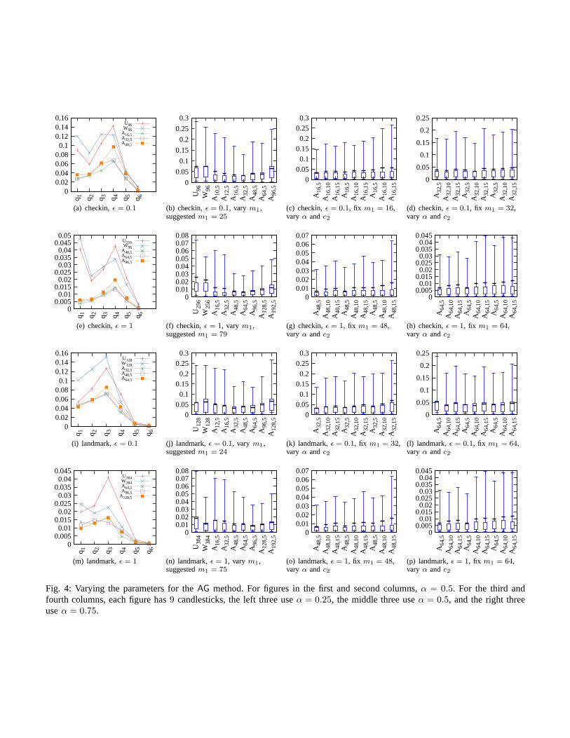
Figure 4 presents experimental results on the effect ofchoosing different parameters for theAG method. We usecheckin and landmark datasets. The first column shows com-parison of the threeAG methods with best performing gridsizes with the best-performingUG method and the Privletmethod with the same grid size. We show results for differentquery sizes. We see that theAG methods outperformUG andPrivlet across all query sizes.

The second column shows the effect of varyingm1, thefirst-level grid size of theAG method. We see that while theAG method like theUG method is affected bym1, it is lesssensitive tom1 and provides good performance for a widerrange ofm1, and that them1 suggested by Guideline 2 iseither at or close to the optimal size.

The third and the fourth columns explore the effect ofvarying α and c2. In each figure, there are9 candlesticks,divided into3 groups of3 each. The left group usesα = 0.25,the middle group usesα = 0.5, and the right group usesα = 0.75. Within each group, we vary the value ofc2. Ascan be seen, settingc2 = c/2 = 5 as suggested significantlyoutperforms larger values ofc2, namely10 and15. We havealso conducted experiments withc2 values from3 to 9, andthe results (which we did not include in the paper for spacelimitation) show that settingc2 in the range of3 to 7 result inalmost the same accuracy. The effect of varyingα can be seenby comparing the left group of3, with the middle group, andthe right group. We observe that settingα = 0.75 performsworse than the otherα values. Settingα = 0.25 andα = 0.5give very similar results, perhaps withα = 0.25 slightly better.We have also experimented with settingα from 0.1 to 0.9, withincrement of0.1. The results suggest that settingα in the rangeof 0.2 to 0.6 give very similar results. We useα = 0.5 as thedefault value.

D. Final Comparison

In Figure 5 we perform an exhaustive comparison of6methods: KD-hybrid,UG with size giving lowest observedrelative error, Privlet on this grid size,AG with m1 giving low-est observed relative error,UG with suggested size,AG withsuggested size. We use all4 datasets, and twoǫ values (0.1and 1). From these results, we observe thatAG consistentlyand significantly outperforms other methods. We also observethatUG with the suggested grid sizes provides about the sameaccuracy as KD-hybrid, andAG with suggested grid sizesclearly outperforms all non-AG methods. When compared withAG with the experimentally observed best grid size, the resultsare slightly worse but in general quite close.

In Figure 6 we plot the same comparisons, but usingabsolute error, instead of relative error. Here we use logscalefor the candlesticks because the ranges of the absolute errorsare quite large. Again we observe thatAG methods consistentlyand significantly outperforms other methods. It is interestingto note that for the road dataset, we observe thatUG withsuggested sizes outperformUG using sizes optimized for therelative error. Recall that this is the only dataset that hasa large

0 0.02 0.04 0.06 0.08 0.1

0.12 0.14 0.16

q 1 q 2 q 3 q 4 q 5 q 6

U96W96

A16,5A32,5A48,5

(a) checkin,ǫ = 0.1

0

0.05

0.1

0.15

0.2

0.25

0.3

U96

W96

A10

,5A

12,5

A16

,5A

32,5

A48

,5A

64,5

A96

,5

(b) checkin,ǫ = 0.1, vary m1,suggestedm1 = 25

0 0.05 0.1

0.15 0.2

0.25 0.3

A16

,5A

16,1

0A

16,1

5A

16,5

A16

,10

A16

,15

A16

,5A

16,1

0A

16,1

5

(c) checkin,ǫ = 0.1, fix m1 = 16,vary α andc2

0

0.05

0.1

0.15

0.2

0.25

A32

,5A

32,1

0A

32,1

5A

32,5

A32

,10

A32

,15

A32

,5A

32,1

0A

32,1

5

(d) checkin,ǫ = 0.1, fix m1 = 32,vary α andc2

0 0.005 0.01

0.015 0.02

0.025 0.03

0.035 0.04

0.045 0.05

q 1 q 2 q 3 q 4 q 5 q 6

U256W96

A48,5A64,5A96,5

(e) checkin,ǫ = 1

0 0.01 0.02 0.03 0.04 0.05 0.06 0.07 0.08

U25

6W

256

A16

,5A

32,5

A48

,5A

64,5

A96

,5A

128,

5A

192,

5

(f) checkin, ǫ = 1, vary m1,suggestedm1 = 79

0 0.01 0.02 0.03 0.04 0.05 0.06 0.07

A48

,5A

48,1

0A

48,1

5A

48,5

A48

,10

A48

,15

A48

,5A

48,1

0A

48,1

5

(g) checkin,ǫ = 1, fix m1 = 48,vary α andc2

0 0.005 0.01

0.015 0.02

0.025 0.03

0.035 0.04

0.045

A64

,5A

64,1

0A

64,1

5A

64,5

A64

,10

A64

,15

A64

,5A

64,1

0A

64,1

5

(h) checkin,ǫ = 1, fix m1 = 64,vary α andc2

0 0.02 0.04 0.06 0.08 0.1

0.12 0.14 0.16

q 1 q 2 q 3 q 4 q 5 q 6

U128W128A32,5A48,5A64,5

(i) landmark,ǫ = 0.1

0 0.05 0.1

0.15 0.2

0.25 0.3

U12

8W

128

A12

,5A

16,5

A32

,5A

48,5

A64

,5A

96,5

A12

8,5

(j) landmark,ǫ = 0.1, vary m1,suggestedm1 = 24

0 0.05 0.1

0.15 0.2

0.25 0.3

A32

,5A

32,1

0A

32,1

5A

32,5

A32

,10

A32

,15

A32

,5A

32,1

0A

32,1

5

(k) landmark,ǫ = 0.1, fix m1 = 32,vary α andc2

0

0.05

0.1

0.15

0.2

0.25

A64

,5A

64,1

0A

64,1

5A

64,5

A64

,10

A64

,15

A64

,5A

64,1

0A

64,1

5

(l) landmark,ǫ = 0.1, fix m1 = 64,vary α andc2

0 0.005 0.01

0.015 0.02

0.025 0.03

0.035 0.04

0.045

q 1 q 2 q 3 q 4 q 5 q 6

U384W384A64,5A96,5

A128,5

(m) landmark,ǫ = 1

0 0.01 0.02 0.03 0.04 0.05 0.06 0.07 0.08

U38

4W

384

A16

,5A

32,5

A48

,5A

64,5

A96

,5A

128,

5A

192,

5

(n) landmark,ǫ = 1, vary m1,suggestedm1 = 75

0 0.01 0.02 0.03 0.04 0.05 0.06 0.07

A48

,5A

48,1

0A

48,1

5A

48,5

A48

,10

A48

,15

A48

,5A

48,1

0A

48,1

5

(o) landmark,ǫ = 1, fix m1 = 48,vary α andc2

0 0.005 0.01

0.015 0.02

0.025 0.03

0.035 0.04

0.045

A64

,5A

64,1

0A

64,1

5A

64,5

A64

,10

A64

,15

A64

,5A

64,1

0A

64,1

5

(p) landmark,ǫ = 1, fix m1 = 64,vary α andc2

Fig. 4: Varying the parameters for theAG method. For figures in the first and second columns,α = 0.5. For the third andfourth columns, each figure has9 candlesticks, the left three useα = 0.25, the middle three useα = 0.5, and the right threeuseα = 0.75.

0

0.05

0.1

0.15

0.2

0.25

0.3

q 1 q 2 q 3 q 4 q 5 q 6

KhyU48W48

A16,5U126A32,5

(a) road,ǫ = 0.1

0 0.05 0.1

0.15 0.2

0.25 0.3

0.35 0.4

Khy

U48

W48

A16

,5

U12

6

A32

,5

(b) road,ǫ = 0.1

0

0.02

0.04

0.06

0.08

0.1

0.12

0.14

q 1 q 2 q 3 q 4 q 5 q 6

KhyU96W96

A32,5U400

A100,5

(c) road,ǫ = 1

0 0.02 0.04 0.06 0.08 0.1

0.12 0.14

Khy

U96

W96

A32

,5

U40

0

A10

0,5

(d) road,ǫ = 1

0 0.02 0.04 0.06 0.08 0.1

0.12 0.14 0.16

q 1 q 2 q 3 q 4 q 5 q 6

KhyU96W96

A32,5U100

A25,5

(e) checkin,ǫ = 0.1

0

0.05

0.1

0.15

0.2

0.25

0.3

Khy

U96

W96

A32

,5

U10

0

A25

,5

(f) checkin, ǫ = 0.1

0 0.005 0.01

0.015 0.02

0.025 0.03

0.035 0.04

0.045 0.05

q 1 q 2 q 3 q 4 q 5 q 6

KhyU256W256A64,5U316

A79,5

(g) checkin,ǫ = 1

0 0.01 0.02 0.03 0.04 0.05 0.06 0.07 0.08 0.09

Khy

U25

6

W25

6

A64

,5

U31

6

A79

,5

(h) checkin,ǫ = 1

0 0.02 0.04 0.06 0.08 0.1

0.12 0.14 0.16 0.18

q 1 q 2 q 3 q 4 q 5 q 6

KhyU128W128A32,5U95

A24,5

(i) landmark,ǫ = 0.1

0 0.05 0.1

0.15 0.2

0.25 0.3

0.35

Khy

U12

8

W12

8

A32

,5

U95

A24

,5

(j) landmark,ǫ = 0.1

0 0.005 0.01

0.015 0.02

0.025 0.03

0.035 0.04

0.045 0.05

q 1 q 2 q 3 q 4 q 5 q 6

KhyU384W384A64,5U300

A75,5

(k) landmark,ǫ = 1

0 0.01 0.02 0.03 0.04 0.05 0.06 0.07 0.08 0.09

Khy

U38

4

W38

4

A64

,5

U30

0

A75

,5

(l) landmark,ǫ = 1

0

0.5

1

1.5

2

2.5

3

3.5

q 1 q 2 q 3 q 4 q 5 q 6

KhyU16W16

A16,5U10

A10,5

(m) storage,ǫ = 0.1

0 1 2 3 4 5 6 7 8

Khy

U16

W16

A16

,5

U10

A10

,5

(n) storage,ǫ = 0.1

0 0.1 0.2 0.3 0.4 0.5 0.6 0.7 0.8 0.9

1

q 1 q 2 q 3 q 4 q 5 q 6KhyU48W48

A32,5U30A10

(o) storage,ǫ = 1

0 0.2 0.4 0.6 0.8

1 1.2 1.4 1.6 1.8

2

Khy

U48

W48

A32

,5

U30

A10

,5

(p) storage,ǫ = 1

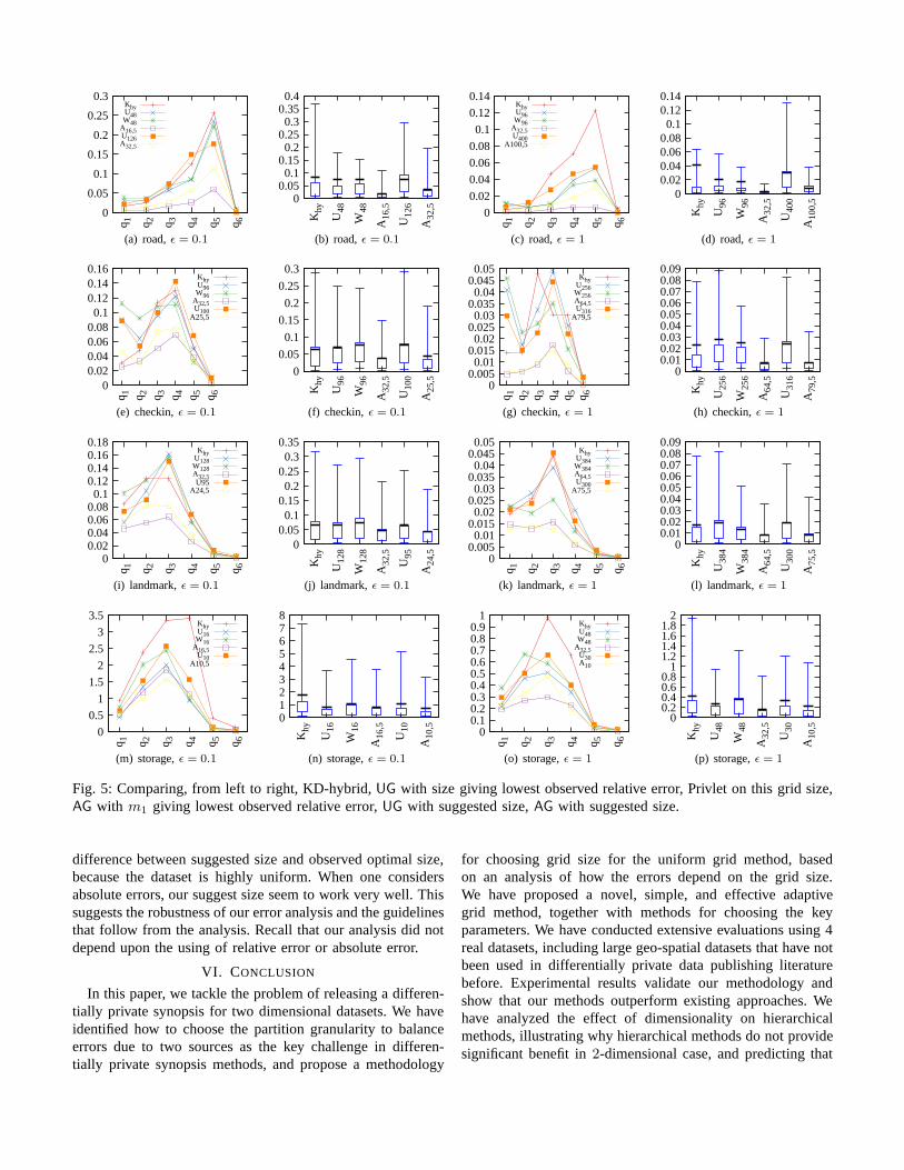
Fig. 5: Comparing, from left to right, KD-hybrid,UG with size giving lowest observed relative error, Privlet onthis grid size,AG with m1 giving lowest observed relative error,UG with suggested size,AG with suggested size.

difference between suggested size and observed optimal size,because the dataset is highly uniform. When one considersabsolute errors, our suggest size seem to work very well. Thissuggests the robustness of our error analysis and the guidelinesthat follow from the analysis. Recall that our analysis did notdepend upon the using of relative error or absolute error.

VI. CONCLUSION

In this paper, we tackle the problem of releasing a differen-tially private synopsis for two dimensional datasets. We haveidentified how to choose the partition granularity to balanceerrors due to two sources as the key challenge in differen-tially private synopsis methods, and propose a methodology

for choosing grid size for the uniform grid method, basedon an analysis of how the errors depend on the grid size.We have proposed a novel, simple, and effective adaptivegrid method, together with methods for choosing the keyparameters. We have conducted extensive evaluations using4real datasets, including large geo-spatial datasets that have notbeen used in differentially private data publishing literaturebefore. Experimental results validate our methodology andshow that our methods outperform existing approaches. Wehave analyzed the effect of dimensionality on hierarchicalmethods, illustrating why hierarchical methods do not providesignificant benefit in2-dimensional case, and predicting that

1

10

100

1000

10000

Khy

U48

W48

A16

,5

U12

6

A32

,5(a) road,ǫ = 0.1

1

10

100

1000

10000

Khy

U96

W96

A32

,5

U40

0

A10

0,5

(b) road,ǫ = 1

10

100

1000

10000

Khy

U96

W96

A32

,5

U10

0

A25

,5

(c) checkin,ǫ = 0.1

1

10

100

1000

10000

Khy

U25

6

W25

6

A64

,5

U31

6

A79

,5

(d) checkin,ǫ = 0.1

10

100

1000

10000

Khy

U12

8

W12

8

A32

,5

U95

A24

,5

(e) landmark,ǫ = 0.1

1

10

100

1000

Khy

U38

4

W38

4

A64

,5

U30

0

A75

,5

(f) landmark,ǫ = 1

1

10

100

1000

10000

Khy

U16

W16

A16

,5

U10

A10

,5

(g) storage,ǫ = 0.1

1

10

100

1000

Khy

U48

W48

A32

,5

U30

A10

,5

(h) storage,ǫ = 1

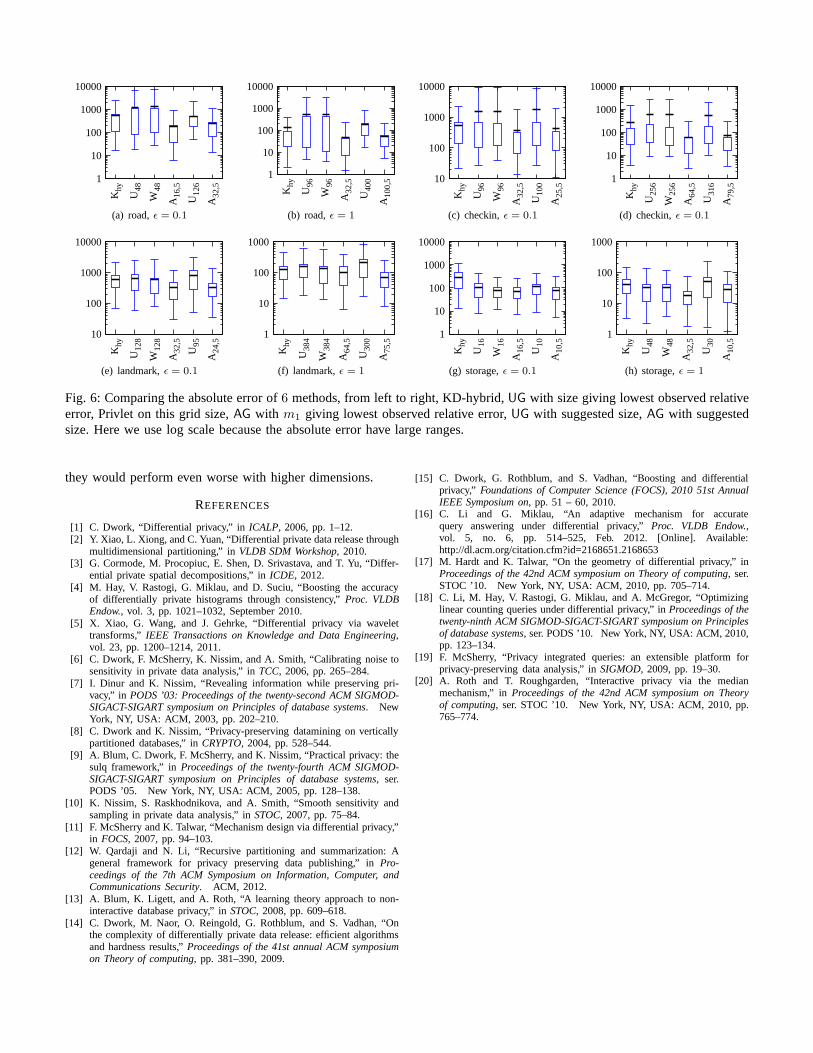
Fig. 6: Comparing the absolute error of6 methods, from left to right, KD-hybrid,UG with size giving lowest observed relativeerror, Privlet on this grid size,AG with m1 giving lowest observed relative error,UG with suggested size,AG with suggestedsize. Here we use log scale because the absolute error have large ranges.

they would perform even worse with higher dimensions.

REFERENCES

[1] C. Dwork, “Differential privacy,” in ICALP, 2006, pp. 1–12.[2] Y. Xiao, L. Xiong, and C. Yuan, “Differential private data release through

multidimensional partitioning,” inVLDB SDM Workshop, 2010.[3] G. Cormode, M. Procopiuc, E. Shen, D. Srivastava, and T. Yu, “Differ-

ential private spatial decompositions,” inICDE, 2012.[4] M. Hay, V. Rastogi, G. Miklau, and D. Suciu, “Boosting theaccuracy

of differentially private histograms through consistency,” Proc. VLDBEndow., vol. 3, pp. 1021–1032, September 2010.

[5] X. Xiao, G. Wang, and J. Gehrke, “Differential privacy via wavelettransforms,”IEEE Transactions on Knowledge and Data Engineering,vol. 23, pp. 1200–1214, 2011.

[6] C. Dwork, F. McSherry, K. Nissim, and A. Smith, “Calibrating noise tosensitivity in private data analysis,” inTCC, 2006, pp. 265–284.

[7] I. Dinur and K. Nissim, “Revealing information while preserving pri-vacy,” in PODS ’03: Proceedings of the twenty-second ACM SIGMOD-SIGACT-SIGART symposium on Principles of database systems. NewYork, NY, USA: ACM, 2003, pp. 202–210.

[8] C. Dwork and K. Nissim, “Privacy-preserving dataminingon verticallypartitioned databases,” inCRYPTO, 2004, pp. 528–544.

[9] A. Blum, C. Dwork, F. McSherry, and K. Nissim, “Practicalprivacy: thesulq framework,” inProceedings of the twenty-fourth ACM SIGMOD-SIGACT-SIGART symposium on Principles of database systems, ser.PODS ’05. New York, NY, USA: ACM, 2005, pp. 128–138.

[10] K. Nissim, S. Raskhodnikova, and A. Smith, “Smooth sensitivity andsampling in private data analysis,” inSTOC, 2007, pp. 75–84.

[11] F. McSherry and K. Talwar, “Mechanism design via differential privacy,”in FOCS, 2007, pp. 94–103.

[12] W. Qardaji and N. Li, “Recursive partitioning and summarization: Ageneral framework for privacy preserving data publishing,” in Pro-ceedings of the 7th ACM Symposium on Information, Computer,andCommunications Security. ACM, 2012.

[13] A. Blum, K. Ligett, and A. Roth, “A learning theory approach to non-interactive database privacy,” inSTOC, 2008, pp. 609–618.

[14] C. Dwork, M. Naor, O. Reingold, G. Rothblum, and S. Vadhan, “Onthe complexity of differentially private data release: efficient algorithmsand hardness results,”Proceedings of the 41st annual ACM symposiumon Theory of computing, pp. 381–390, 2009.

[15] C. Dwork, G. Rothblum, and S. Vadhan, “Boosting and differentialprivacy,” Foundations of Computer Science (FOCS), 2010 51st AnnualIEEE Symposium on, pp. 51 – 60, 2010.

[16] C. Li and G. Miklau, “An adaptive mechanism for accuratequery answering under differential privacy,”Proc. VLDB Endow.,vol. 5, no. 6, pp. 514–525, Feb. 2012. [Online]. Available:http://dl.acm.org/citation.cfm?id=2168651.2168653

[17] M. Hardt and K. Talwar, “On the geometry of differentialprivacy,” inProceedings of the 42nd ACM symposium on Theory of computing, ser.STOC ’10. New York, NY, USA: ACM, 2010, pp. 705–714.

[18] C. Li, M. Hay, V. Rastogi, G. Miklau, and A. McGregor, “Optimizinglinear counting queries under differential privacy,” inProceedings of thetwenty-ninth ACM SIGMOD-SIGACT-SIGART symposium on Principlesof database systems, ser. PODS ’10. New York, NY, USA: ACM, 2010,pp. 123–134.

[19] F. McSherry, “Privacy integrated queries: an extensible platform forprivacy-preserving data analysis,” inSIGMOD, 2009, pp. 19–30.

[20] A. Roth and T. Roughgarden, “Interactive privacy via the medianmechanism,” inProceedings of the 42nd ACM symposium on Theoryof computing, ser. STOC ’10. New York, NY, USA: ACM, 2010, pp.765–774.