Chapter 5 Collection and Analysis of Rate Data

Two common types of reactors for obtaining kinetics data: Batch & Differential reactors

Seven methods for data analyses: (1) Differential method; (2) Integration method; (3) Half-life

method; (4) Initial-rate method; (5) Linear regression method; (6) Non-linear regression

method; (7) Excess method.

§ Batch Reactors

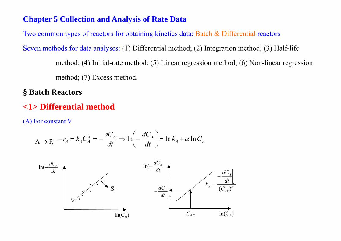
<1> Differential method (A) For constant V

A → P, AAAA

AAA Ckdt

dCdt

dCCkr lnlnln αα +=

−⇒−==−

α)( AP

P

A

A Cdt

dC

k−

=

ln(dt

dCA−

ln(CA)

S =α

ln(dt

dCA−

ln(CA) CAP

P

A

dtdC

−

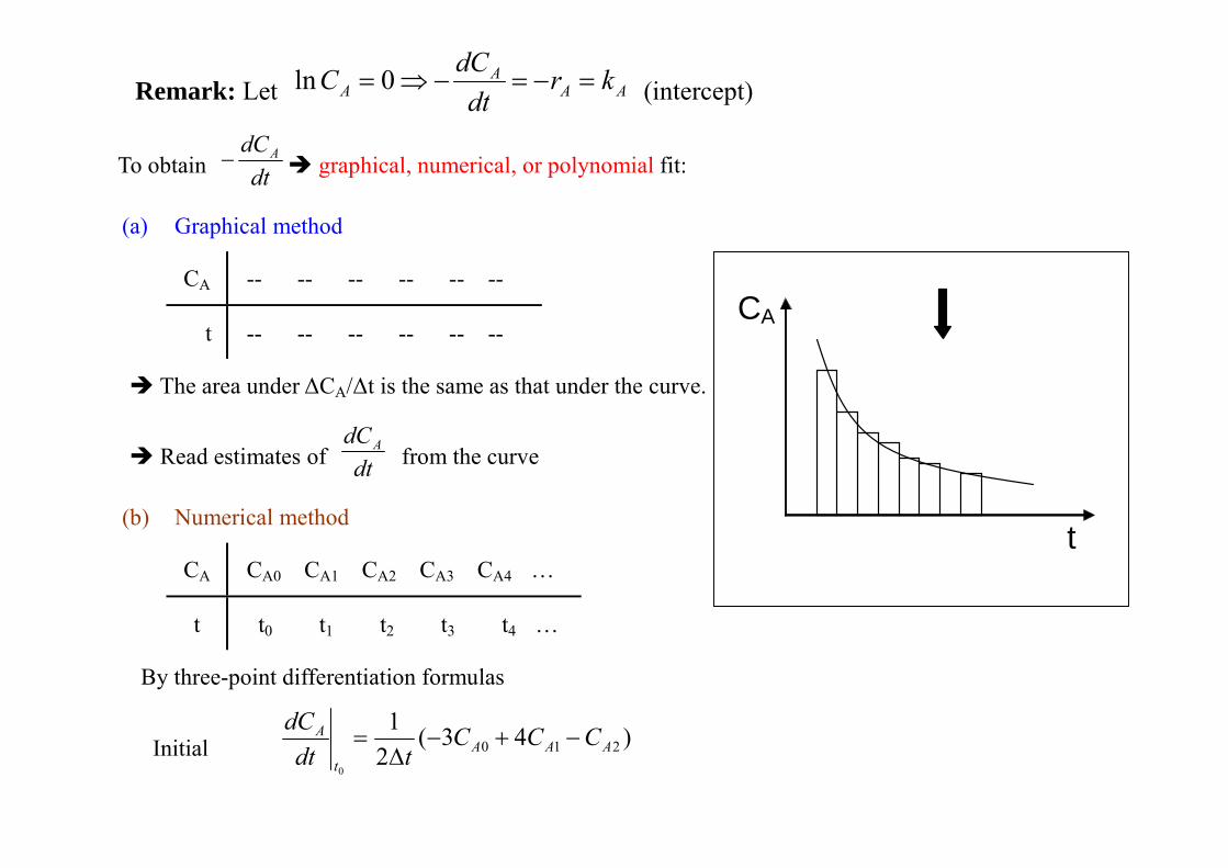
Remark: Let AAA

A krdt

dCC =−=−⇒= 0ln (intercept)

To obtain dtdCA− graphical, numerical, or polynomial fit:

(a) Graphical method

CA -- -- -- -- -- --

t -- -- -- -- -- --

The area under ∆CA/∆t is the same as that under the curve.

Read estimates of dtdCA from the curve

(b) Numerical method

CA CA0 CA1 CA2 CA3 CA4 …

t t0 t1 t2 t3 t4 …

By three-point differentiation formulas

Initial： )43(21

2100

AAAt

A CCCtdt

dC−+−

∆=

CA

t

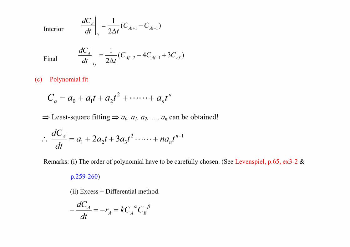
Interior： )(21

11 −+ −∆

= AiAit

A CCtdt

dC

i

Final： )34(21

12 AfAfAft

A CCCtdt

dC

f

+−∆

= −−

(c) Polynomial fit

nna tatataaC ++++= LL2

210

⇒ Least-square fitting ⇒ a0, a1, a2, …, an can be obtained!

12321 32 −+++=∴ n

nA tnatataa

dtdC

LL

Remarks: (i) The order of polynomial have to be carefully chosen. (See Levenspiel, p.65, ex3-2 &

p.259-260)

(ii) Excess + Differential method.

βαBAA

A CkCrdt

dC=−=−

ββαβα

ααββα

BBABAA

AABA

AABBAA

BBAB

CkCkCCkCr

constantCCCCbCkCkCCkCr

constantCCCCa

''0

000

'0

000

)(

)(

===−⇒

=≈⇒>>===−⇒

=≈⇒>>

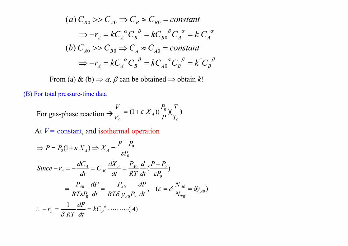
From (a) & (b) ⇒ α, β can be obtained ⇒ obtain k!

(B) For total pressure-time data

For gas-phase reaction ))()(1(0

0

0 TT

PP

XVV

Aε+=

At V = constant, and isothermal operation

)(1

)(,

)(

)1(

00

0

00

0

0

0

0

000

0

00

AkCdtdP

RTr

yNN

dtdP

PyRTP

dtdP

PRTP

PPP

dtd

RTP

dtdXC

dtdCrSince

PPPXXPP

AA

AT

A

A

AA

AAA

AA

AA

LLLα

δ

δδεδε

ε

εε

==−∴

====

−==−=−

−=⇒+=⇒

)260.,1.5.()(),(

]/)[()1()1( 00

0

000

pExSeePfdtdPA

RTPPP

PPP

RTPXCC AA

AAA

=⇒

−−=

−−=−=

代入式

又δ

εQ

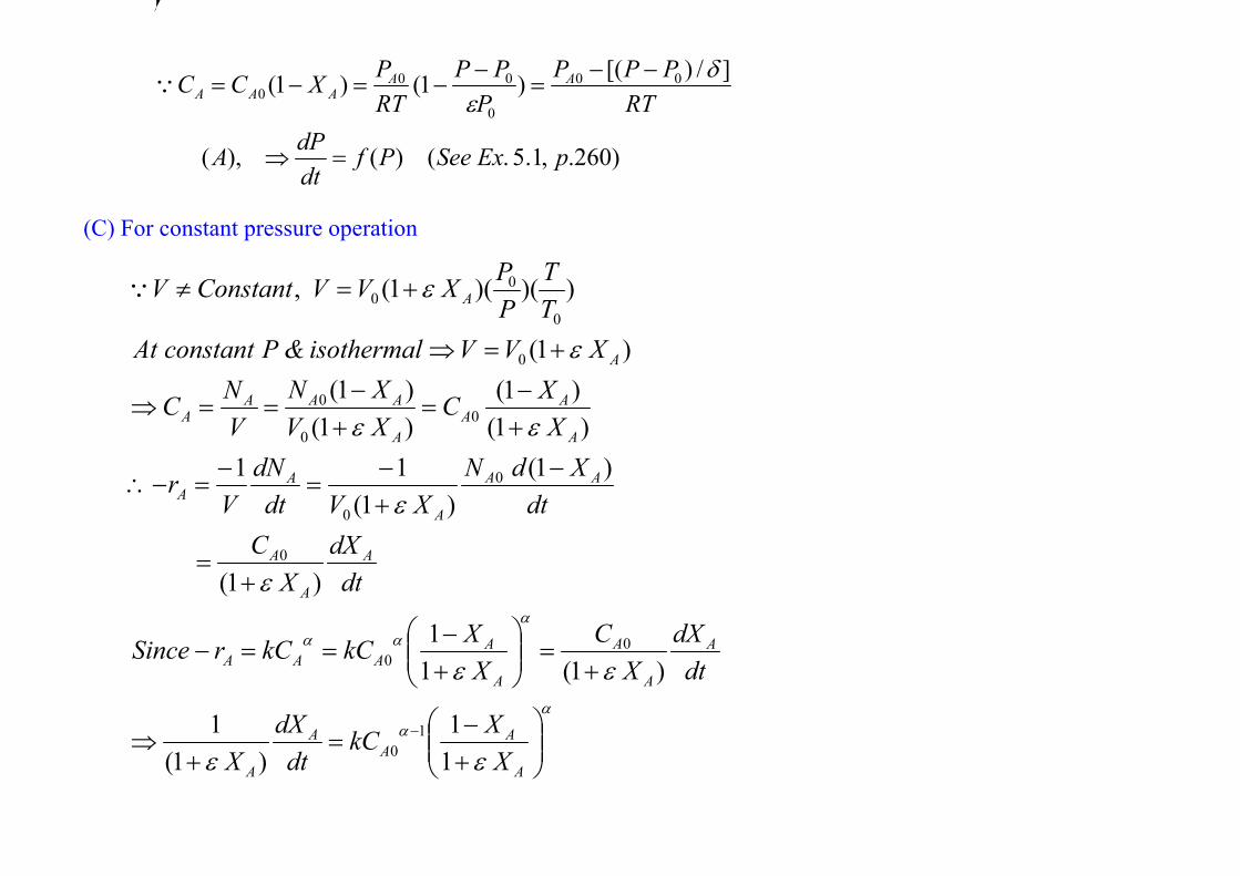
(C) For constant pressure operation

αα

ααα

εε

εε

ε

ε

εε

ε

ε

+−

=+

⇒

+=

+−

==−

+=

−+−

=−

=−∴

+−

=+−

==⇒

+=⇒

+=≠

−

A

AA

A

A

A

A

A

A

AAAA

A

A

A

AA

A

AA

A

AA

A

AAAA

A

A

XXkC

dtdX

X

dtdX

XC

XXkCkCrSince

dtdX

XC

dtXdN

XVdtdN

Vr

XXC

XVXN

VNC

XVVisothermal&PconstantAtTT

PPXVVConstantV

11

)1(1

)1(11

)1(

)1()1(

11)1(

)1()1()1(

)1(

))()(1(,

10

00

0

0

0

00

0

0

0

00Q

t

XA

dtdX ASlope =

kCX

Xdt

dXX A

A

AA

A

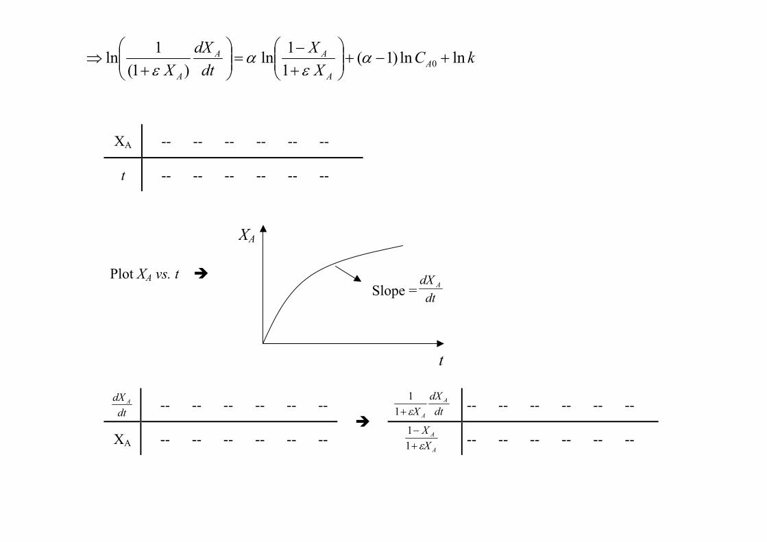
lnln)1(11ln

)1(1ln 0 +−+

+−

=

+

⇒ αε

αε

XA -- -- -- -- -- --

t -- -- -- -- -- --

Plot XA vs. t

dtdX A -- -- -- -- -- -- dt

dXX

A

Aε+11

-- -- -- -- -- --

XA -- -- -- -- -- --

A

A

XXε+−

11 -- -- -- -- -- --

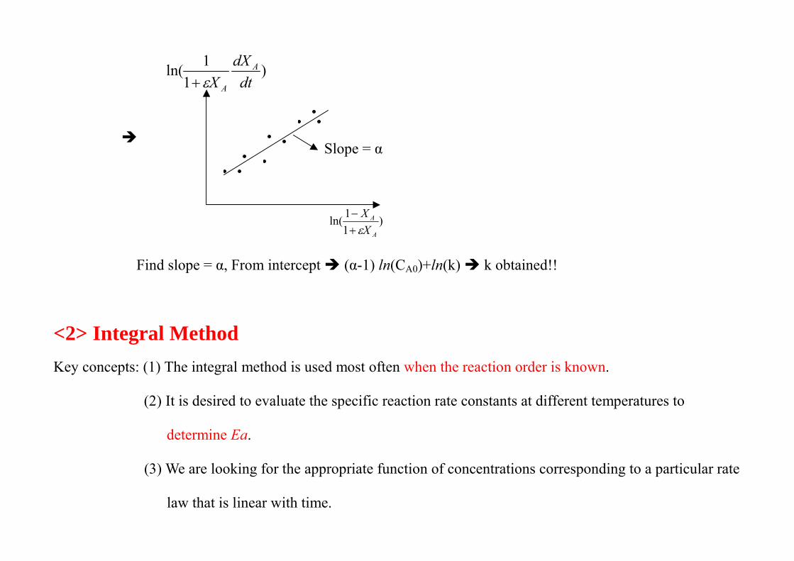
Slope = α

)11ln(

A

A

XXε+−

)1

1ln(dt

dXX

A

Aε+

Find slope = α, From intercept (α-1) ln(CA0)+ln(k) k obtained!!

<2> Integral Method Key concepts: (1) The integral method is used most often when the reaction order is known.

(2) It is desired to evaluate the specific reaction rate constants at different temperatures to

determine Ea.

(3) We are looking for the appropriate function of concentrations corresponding to a particular rate

law that is linear with time.

Slope = -k

t

CA

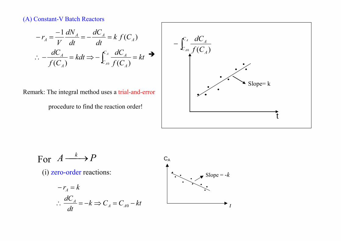
(A) Constant-V Batch Reactors

∫ =−⇒=−∴

=−=−

=−

A

A

C

CA

A

A

A

AAA

A

ktCf

dCkdtCf

dC

Cfkdt

dCdt

dNV

r

0 )()(

)(1

Remark: The integral method uses a trial-and-error

procedure to find the reaction order!

For PA k→ (i) zero-order reactions:

ktCCkdt

dCkr

AAA

A

−=⇒−=∴

=−

0

Slope= k

∫−A

A

C

CA

A

CfdC

0 )(

t

Slope = k

t

A

A

CC 0ln

S = k

t

AX−11ln

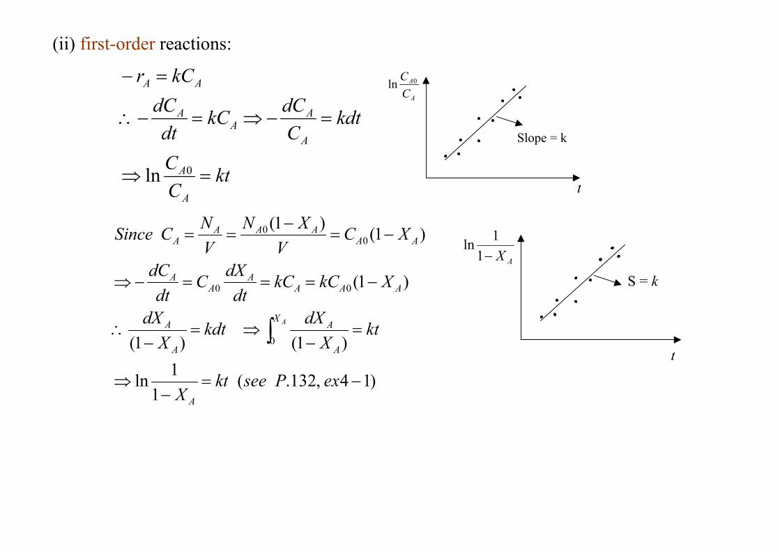
(ii) first-order reactions:

kt

CC

kdtCdCkC

dtdC

kCr

A

A

A

AA

A

AA

=⇒

=−⇒=−∴

=−

0ln

)14,132.(1

1ln

)1()1(

)1(

)1()1(

0

00

00

−=−

⇒

=−

⇒=−

∴

−===−⇒

−=−

==

∫

exPseektX

ktX

dXkdtX

dX

XkCkCdt

dXCdt

dC

XCV

XNVNCSince

A

X

A

A

A

A

AAAA

AA

AAAAA

A

A

S = k

t

AC1

0

1

AC

Slope= CA0 k

t

A

A

XX−1

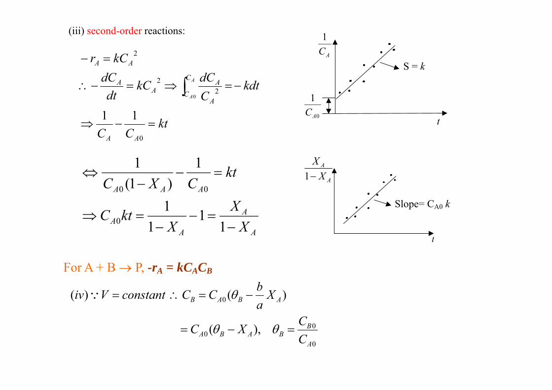
(iii) second-order reactions:

ktCC

kdtCdCkC

dtdC

kCr

AA

C

CA

AA

A

AA

A

A

=−⇒

−=⇒=−∴

=−

∫

0

22

2

11

0

A

A

AA

AAA

XX

XktC

ktCXC

−=−

−=⇒

=−−

⇔

11

11

1)1(

1

0

00

For A + B → P, -rA = kCACB

0

00

0

),(

)()(

A

BBABA

ABAB

CCXC

XabCCconstantViv

=−=

−=∴=

θθ

θQ

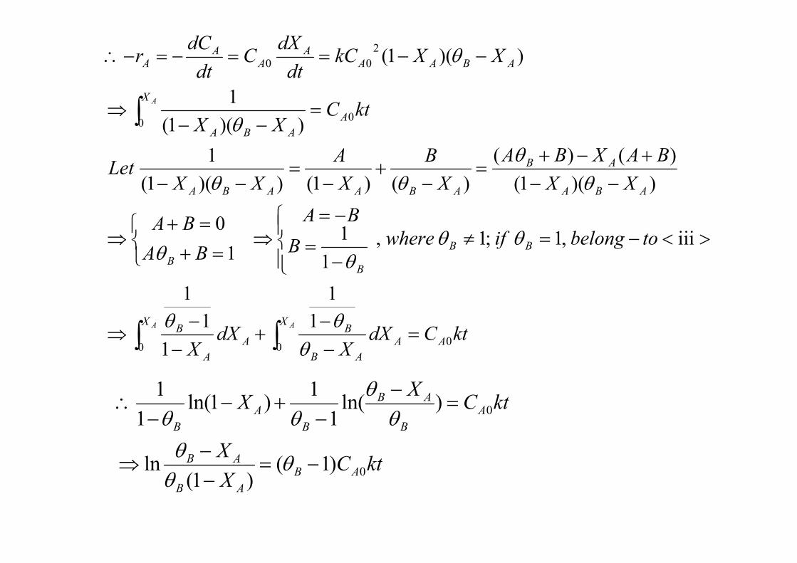
ktCdXX

dXX

tobelongifwhereBBA

BABA

XXBAXBA

XB

XA

XXLet

ktCXX

XXkCdt

dXCdt

dCr

AA

X

AB

BA

X

A

B

BB

BB

ABA

AB

ABAABA

A

X

ABA

ABAAA

AA

A

AA

A

000

00

200

11

11

1

iii,1;1,1

11

0

))(1()()(

)()1())(1(1

))(1(1

))(1(

=−−

+−−

⇒

><−=≠

−=

−=⇒

=+=+

⇒

−−+−+

=−

+−

=−−

=−−

⇒

−−==−=−∴

∫∫

∫

θθθ

θθθθ

θθ

θθ

θ

θ

ktCXX

ktCXX

ABAB

AB

AB

AB

BA

B

0

0

)1()1(

ln

)ln(1

1)1ln(1

1

−=−−

⇒

=−

−+−

−∴

θθθ

θθ

θθ

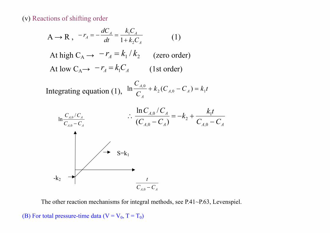
(v) Reactions of shifting order

A → R , A

AAA Ck

Ckdt

dCr2

1

1+=−=− (1)

At high CA → 21 / kkrA =− (zero order)

At low CA→ AA Ckr 1=− (1st order)

Integrating equation (1), tkCCkC

CAA

A

A10,2

0, )(ln =−+

AA

AA

CCCC−0,

0, /ln

AAAA

AA

CCtkk

CCCC

−+−=

−∴

0,

12

0,

0,

)(/ln

AA CCt−0,

☆ The other reaction mechanisms for integral methods, see P.41~P.63, Levenspiel.

(B) For total pressure-time data (V = V0, T = T0)

-k2

S=k1

RT

PadP

ac

RT

PPadP

XadCC

RT

PacP

ac

RT

PPacP

XacCC

RT

PabP

ab

RT

PPabP

XabCC

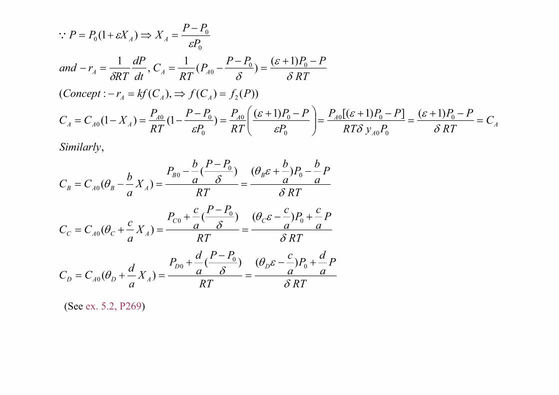
Similarly

CRT

PPPyRT

PPPP

PPRTP

PPP

RTPXCC

PfCfCkfrConceptRT

PPPPPRT

CdtdP

RTrand

PPPXXPP

DD

ADAD

CC

ACAC

BB

ABAB

AA

AAAAAA

AAA

AAA

AA

δ

εθδθ

δ

εθδθ

δ

εθδθ

δε

δε

εε

ε

δε

δδ

εε

+−=

−+

=+=

+−=

−+

=+=

−+=

−−

=−=

=−+

=−+

=

−+=

−−=−=

=⇒=−

−+=

−−==−

−=⇒+=

00

0

0

00

0

0

00

0

0

0

00

00

0

00

0

000

2

000

0

00

)()()(

)()()(

)()()(

,

)1(])1[()1()1()1(

))()(),(:(

)1()(1,1

)1(Q

(See ex. 5.2, P269)

Slope= kδRT

t

∫P

P PfdP

0 )(2

Slope= k

t

)1ln(0A

A XC εε

+

tvs

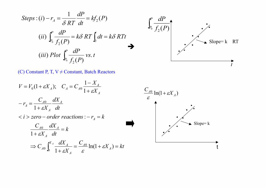
PfdPPlotiii

RTtkdtRTkPf

dPii

PkfdtdP

RTriSteps

P

P

tP

P

A

.)(

)(

)()(

)(1)(:

0

0

2

02

2

∫

∫∫ ==

==−

δδ

δ

(C) Constant P, T, V ≠ Constant, Batch Reactors

ktXCX

dXC

kdt

dXX

Ckrreactionsorderzeroi

dtdX

XCr

XXCCXVV

AA

X

A

AA

A

A

A

A

A

A

AA

A

AAAA

A =+=+

⇒

=+

=−−><+

=−

+−

=+=

∫ )1ln(1

1

:1

11);1(

000

0

0

00

εεε

ε

ε

εε

ktXXXkC

dtdX

XC

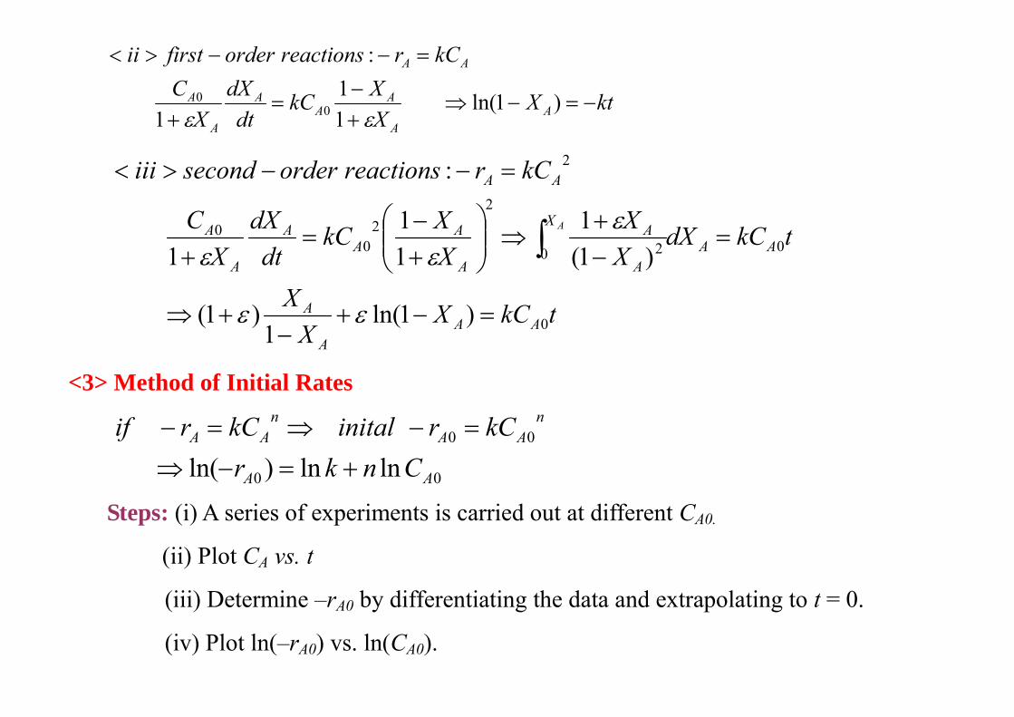
kCrreactionsorderfirstii

AA

AA

A

A

A

AA

−=−⇒+−

=+

=−−><

)1ln(11

1

:

00

εε

tkCXX

X

tkCdXXX

XXkC

dtdX

XC

kCrreactionsordersecondiii

AAA

A

AA

X

A

A

A

AA

A

A

A

AA

A

0

00 2

22

00

2

)1ln(1

)1(

)1(1

11

1

:

=−+−

+⇒

=−+

⇒

+−

=+

=−−><

∫

εε

εεε

<3> Method of Initial Rates

00

00

lnln)ln( AA

nAA

nAA

CnkrkCrinitalkCrif

+=−⇒=−⇒=−

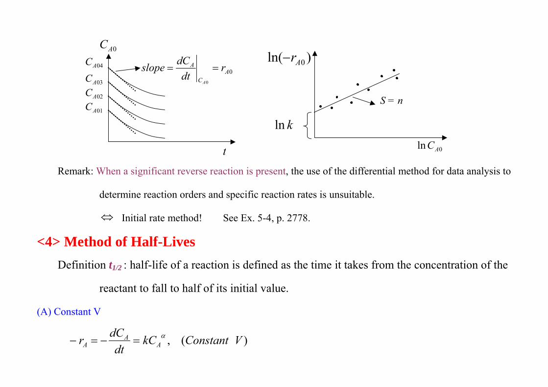
Steps: (i) A series of experiments is carried out at different CA0.

(ii) Plot CA vs. t

(iii) Determine –rA0 by differentiating the data and extrapolating to t = 0.

(iv) Plot ln(–rA0) vs. ln(CA0).

S = n

kln

)ln( 0Ar−

0ln ACt

0AC

01AC02AC03AC04AC

00

AC

A rdt

dCslopeA

==

Remark: When a significant reverse reaction is present, the use of the differential method for data analysis to

determine reaction orders and specific reaction rates is unsuitable.

⇔ Initial rate method! See Ex. 5-4, p. 2778.

<4> Method of Half-Lives Definition t1/2 : half-life of a reaction is defined as the time it takes from the concentration of the

reactant to fall to half of its initial value.

(A) Constant V

)(, VConstantkCdt

dCr AA

Aα=−=−

S = 1-α

0ln AC)1(12ln

1

−−−

α

α

k

1/2tln

A0

1

2/11A0

1

/1

1A0

1

2/1A02/1

1

A

A01

A01

A01

A

1A0

1A

C)1()1(12lnln,

C1

)1(1,

C1

)1(12C

21,

1CC

)1(C1

C1

C1

)1(1

,)1(CC

ααα

α

αα

α

α

α

α

α

α

α

ααα

αα

−+−−

=∴−−

=

−−

=⇒=

−

−

=

−

−=⇒

−=−⇒

−

−

−

−

−

−

−−−

−−

kt

kntSimilarly

ktCtat

kkt

kt

n

A

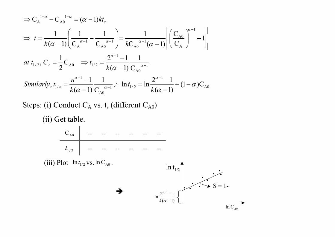
Steps: (i) Conduct CA vs. t, (different CA0)

(ii) Get table.

A0C -- -- -- -- -- --

2/1t -- -- -- -- -- --

(iii) Plot 2/1ln t vs. A0Cln .

(iv) from slope, S = 1 - α, α = 1 - S; and from intercept, I = )1(12ln

1

−−−

α

α

k , k.

Remark: If two reactants are involved in the chemical reaction, use the method of excess

in conjunction with the method of half lives.

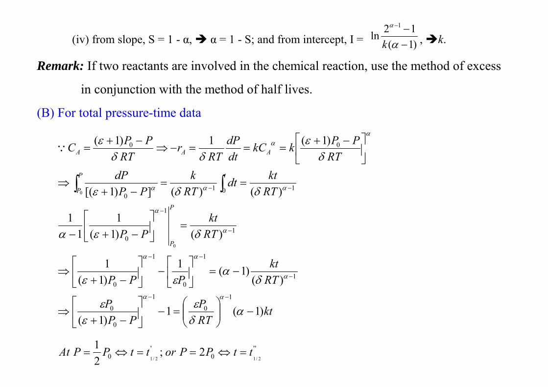
(B) For total pressure-time data

ktRTP

PPP

RTkt

PPP

RTkt

PP

RTktdt

RTk

PPdP

RTPPkkC

dtdP

RTr

RTPPC

P

P

tP

P

AAA

)1(1)1(

)()1(1

)1(1

)()1(1

11

)()(])1[(

)1(1)1(

1

0

1

0

0

1

1

0

1

0

1

1

0

1010

00

0

0

−

=−

−+

⇒

−=

−

−+

⇒

=

−+−

==−+

⇒

−+===−⇒

−+=

−−

−

−−

−

−

−− ∫∫

αδε

εε

δα

εε

δεα

δδε

δε

δδε

αα

α

αα

α

α

ααα

αα

Q

''0

'0 2/12/1

2;21 ttPPorttPPAt =⇔==⇔=

1

11

0''

1

11

0'

101

11

'

1

0'1

)1(

)(11

lnln)1(ln,

)1(

)(112

2

lnln)1(ln

)1(

)(112

2

)1(112

2

2/1

2/1

2/1

2/1

−

−−

−

−−

−−

−−

−−

−

−

++−=

−

−

++−=⇒

−

−

+=⇒

−=−

+⇒

α

αα

α

αα

αα

αα

αα

εα

δεε

α

εα

δεε

α

εα

δεε

δεα

εε

k

RTPtSimilarly

k

RTPt

Pk

RTt

RTPkt

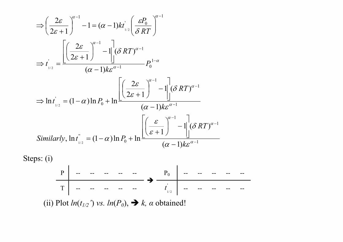
Steps: (i)

P -- -- -- -- -- P0 -- -- -- -- --

T -- -- -- -- -- '2/1

t -- -- -- -- --

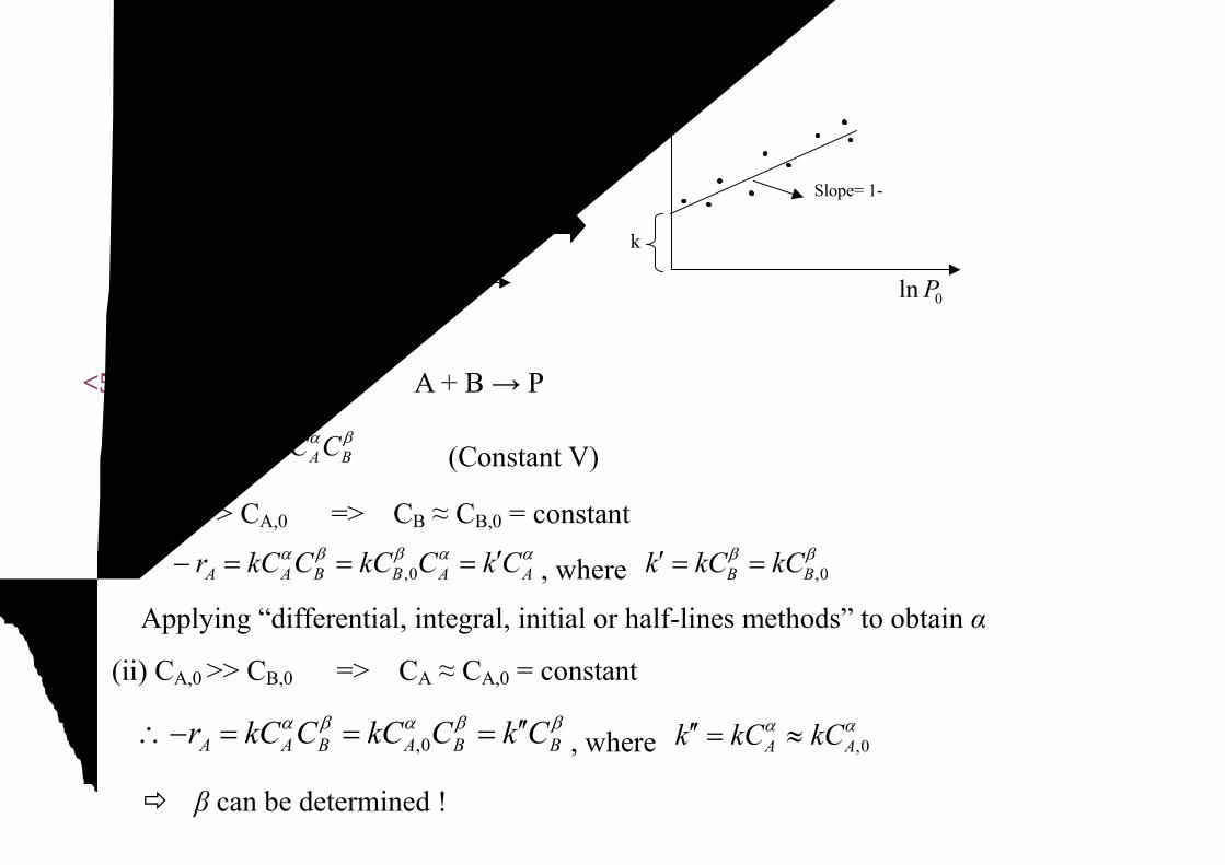
(ii) Plot ln(t1/2’) vs. ln(P0), k, α obtained!

t

0P

01P02P03P04P

'2/1

t

Slope= 1-α

'2/1

ln t

k

0ln P

<5> Method of Excess A + B → P

βαBA

A CCkrdt

dCA =−=− (Constant V)

(i) CB,0 >> CA,0 => CB ≈ CB,0 = constant

∴ααββαAABBAA CkCkCCkCr ′===− 0, , where

ββ0,BB kCkCk ==′

Applying “differential, integral, initial or half-lines methods” to obtain α

(ii) CA,0 >> CB,0 => CA ≈ CA,0 = constant

ββαβαBBABAA CkCkCCkCr ′′===−∴ 0, , where

αα0,AA kCkCk ≈=′′

β can be determined !

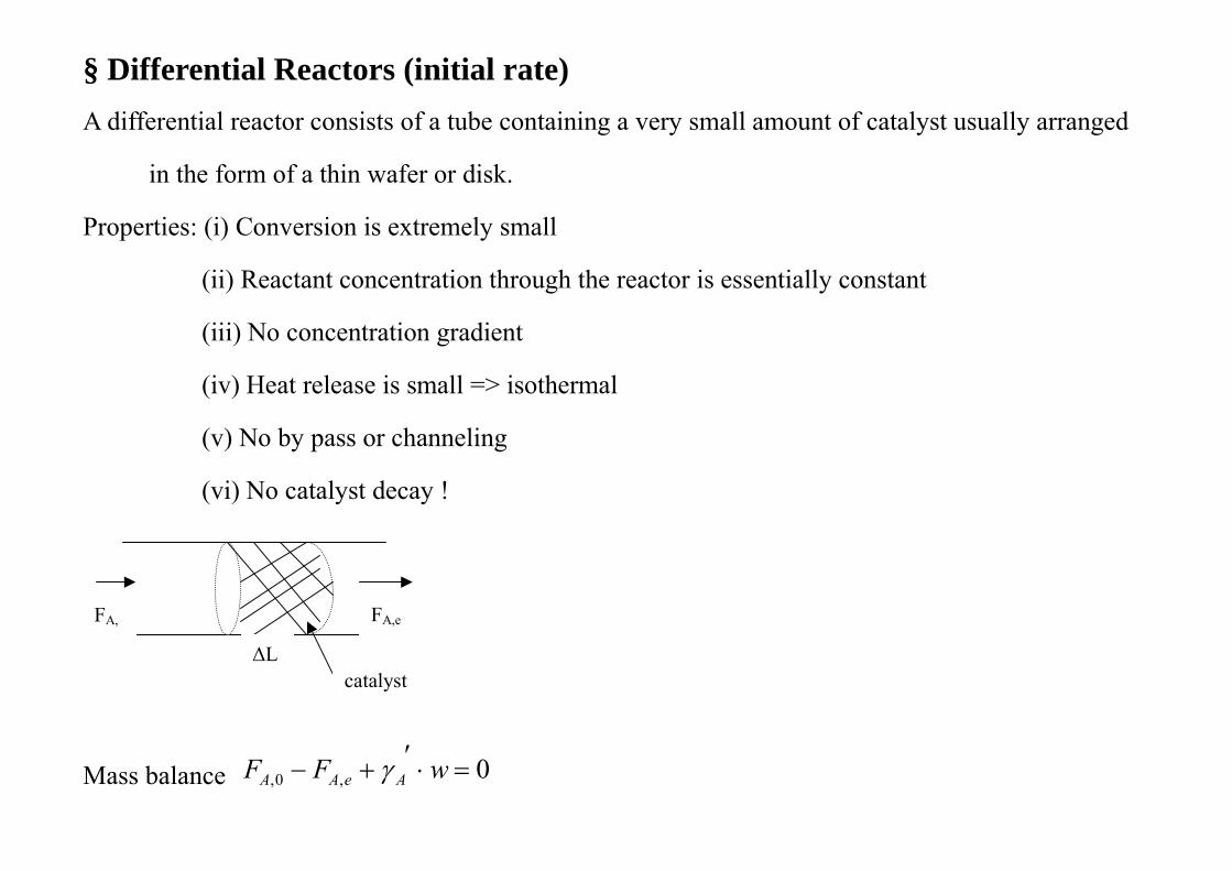
§ Differential Reactors (initial rate) A differential reactor consists of a tube containing a very small amount of catalyst usually arranged

in the form of a thin wafer or disk.

Properties: (i) Conversion is extremely small

(ii) Reactant concentration through the reactor is essentially constant

(iii) No concentration gradient

(iv) Heat release is small => isothermal

(v) No by pass or channeling

(vi) No catalyst decay !

Mass balance 0,0, =⋅′+− wFF AeAA γ

FA, FA,e

∆L catalyst

wXF

wVCCV

r AAeAAA

0,,0,0' =−

=−∴

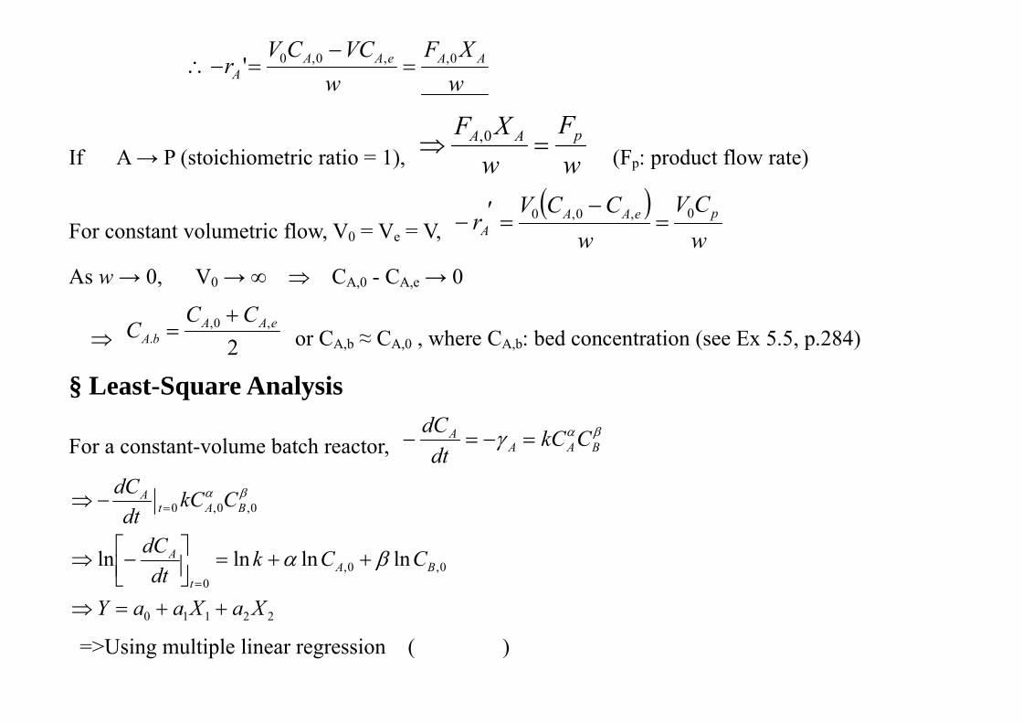
If A → P (stoichiometric ratio = 1), wF

wXF pAA =⇒ 0,

(Fp: product flow rate)

For constant volumetric flow, V0 = Ve = V, ( )

wCV

wCCV

r peAAA

0,0,0 =−

=′−

As w → 0, V0 → ∞ ⇒ CA,0 - CA,e → 0

⇒ 2,0,

.eAA

bACC

C+

= or CA,b ≈ CA,0 , where CA,b: bed concentration (see Ex 5.5, p.284)

§ Least-Square Analysis

For a constant-volume batch reactor, βαγ BAA

A CkCdt

dC=−=−

22110

0,0,0

0,0,0

lnlnlnln

XaXaaY

CCkdt

dC

CkCdt

dC

BAt

A

BAtA

++=⇒

++=

−⇒

−⇒

=

=

βα

βα

=>Using multiple linear regression (利用統計)

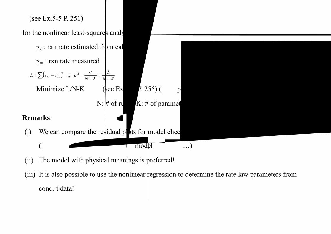
(see Ex.5-5 P. 251)

for the nonlinear least-squares analysis

γc : rxn rate estimated from calculation

γm : rxn rate measured

( )∑ −= 2ii mCL γγ ;

KNL

KNs

−=

−=

22σ

Minimize L/N-K (see Ex. 5.6 P. 255) (先看 p. 253 Table 5-2)

N: # of runs , K: # of parameters

Remarks:

(i) We can compare the residual plots for model checking

(是否缺少某一參數，比較不同 model之適切性…)

(ii) The model with physical meanings is preferred!

(iii) It is also possible to use the nonlinear regression to determine the rate law parameters from

conc.-t data!