Embed Size (px)
Citation preview
Victor Andreevich Toponogovwith the editorial assistance ofVladimir Y. Rovenski
Differential Geometryof Curves and Surfaces
A Concise Guide
BirkhauserBoston • Basel • Berlin

Victor A. Toponogov (deceased)Department of Analysis and GeometrySobolev Institute of MathematicsSiberian Branch of the Russian Academy
of SciencesNovosibirsk-90, 630090Russia
With the editorial assistance of:Vladimir Y. RovenskiDepartment of MathematicsUniversity of HaifaHaifa, Israel
Cover design by Alex Gerasev.
AMS Subject Classification: 53-01, 53Axx, 53A04, 53A05, 53A55, 53B20, 53B21, 53C20, 53C21
Library of Congress Control Number: 2005048111
ISBN-10 0-8176-4384-2 eISBN 0-8176-4402-4ISBN-13 978-0-8176-4384-3
Printed on acid-free paper.
c©2006 Birkhauser BostonAll rights reserved. This work may not be translated or copied in whole or in part without the writ-ten permission of the publisher (Birkhauser Boston, c/o Springer Science+Business Media Inc., 233Spring Street, New York, NY 10013, USA) and the author, except for brief excerpts in connectionwith reviews or scholarly analysis. Use in connection with any form of information storage and re-trieval, electronic adaptation, computer software, or by similar or dissimilar methodology now knownor hereafter developed is forbidden.The use in this publication of trade names, trademarks, service marks and similar terms, even if theyare not identified as such, is not to be taken as an expression of opinion as to whether or not they aresubject to proprietary rights.
Printed in the United States of America. (TXQ/EB)
9 8 7 6 5 4 3 2 1
www.birkhauser.com

Contents
Preface . . . . . . . . . . . . . . . . . . . . . . . . . . . . . . . . . . . . . . . . . . . . . . . . . . . . . . . vii
About the Author . . . . . . . . . . . . . . . . . . . . . . . . . . . . . . . . . . . . . . . . . . . . . . ix
1 Theory of Curves in Three-dimensional Euclidean Space and in thePlane . . . . . . . . . . . . . . . . . . . . . . . . . . . . . . . . . . . . . . . . . . . . . . . . . . . . . . . 11.1 Preliminaries . . . . . . . . . . . . . . . . . . . . . . . . . . . . . . . . . . . . . . . . . . . . . . 11.2 Definition and Methods of Presentation of Curves . . . . . . . . . . . . . . . 21.3 Tangent Line and Osculating Plane . . . . . . . . . . . . . . . . . . . . . . . . . . . . 61.4 Length of a Curve . . . . . . . . . . . . . . . . . . . . . . . . . . . . . . . . . . . . . . . . . . 111.5 Problems: Convex Plane Curves . . . . . . . . . . . . . . . . . . . . . . . . . . . . . . 151.6 Curvature of a Curve . . . . . . . . . . . . . . . . . . . . . . . . . . . . . . . . . . . . . . . . 191.7 Problems: Curvature of Plane Curves . . . . . . . . . . . . . . . . . . . . . . . . . . 241.8 Torsion of a Curve . . . . . . . . . . . . . . . . . . . . . . . . . . . . . . . . . . . . . . . . . . 451.9 The Frenet Formulas and the Natural Equation of a Curve . . . . . . . . . 471.10 Problems: Space Curves . . . . . . . . . . . . . . . . . . . . . . . . . . . . . . . . . . . . . 511.11 Phase Length of a Curve and the Fenchel–Reshetnyak Inequality . . . 561.12 Exercises to Chapter 1 . . . . . . . . . . . . . . . . . . . . . . . . . . . . . . . . . . . . . . 61
2 Extrinsic Geometry of Surfaces in Three-dimensional EuclideanSpace . . . . . . . . . . . . . . . . . . . . . . . . . . . . . . . . . . . . . . . . . . . . . . . . . . . . . . 652.1 Definition and Methods of Generating Surfaces . . . . . . . . . . . . . . . . . 652.2 The Tangent Plane . . . . . . . . . . . . . . . . . . . . . . . . . . . . . . . . . . . . . . . . . . 702.3 First Fundamental Form of a Surface . . . . . . . . . . . . . . . . . . . . . . . . . . 74
vi Contents
2.4 Second Fundamental Form of a Surface . . . . . . . . . . . . . . . . . . . . . . . . 792.5 The Third Fundamental Form of a Surface . . . . . . . . . . . . . . . . . . . . . . 912.6 Classes of Surfaces . . . . . . . . . . . . . . . . . . . . . . . . . . . . . . . . . . . . . . . . . 952.7 Some Classes of Curves on a Surface . . . . . . . . . . . . . . . . . . . . . . . . . . 1142.8 The Main Equations of Surface Theory . . . . . . . . . . . . . . . . . . . . . . . . 1272.9 Appendix: Indicatrix of a Surface of Revolution . . . . . . . . . . . . . . . . . 1392.10 Exercises to Chapter 2 . . . . . . . . . . . . . . . . . . . . . . . . . . . . . . . . . . . . . . 147
3 Intrinsic Geometry of Surfaces . . . . . . . . . . . . . . . . . . . . . . . . . . . . . . . . . 1513.1 Introducing Notation . . . . . . . . . . . . . . . . . . . . . . . . . . . . . . . . . . . . . . . . 1513.2 Covariant Derivative of a Vector Field . . . . . . . . . . . . . . . . . . . . . . . . . 1523.3 Parallel Translation of a Vector along a
Curve on a Surface . . . . . . . . . . . . . . . . . . . . . . . . . . . . . . . . . . . . . . . . . 1533.4 Geodesics . . . . . . . . . . . . . . . . . . . . . . . . . . . . . . . . . . . . . . . . . . . . . . . . . 1563.5 Shortest Paths and Geodesics . . . . . . . . . . . . . . . . . . . . . . . . . . . . . . . . . 1613.6 Special Coordinate Systems . . . . . . . . . . . . . . . . . . . . . . . . . . . . . . . . . . 1723.7 Gauss–Bonnet Theorem and Comparison Theorem for the Angles
of a Triangle . . . . . . . . . . . . . . . . . . . . . . . . . . . . . . . . . . . . . . . . . . . . . . . 1793.8 Local Comparison Theorems for Triangles . . . . . . . . . . . . . . . . . . . . . 1843.9 Aleksandrov Comparison Theorem for the Angles of a Triangle . . . . 1893.10 Problems to Chapter 3 . . . . . . . . . . . . . . . . . . . . . . . . . . . . . . . . . . . . . . . 195
References . . . . . . . . . . . . . . . . . . . . . . . . . . . . . . . . . . . . . . . . . . . . . . . . . . 199
Index . . . . . . . . . . . . . . . . . . . . . . . . . . . . . . . . . . . . . . . . . . . . . . . . . . . . . . . 203
Preface
This concise guide to the differential geometry of curves and surfaces can berecommended to first-year graduate students, strong senior students, and studentsspecializing in geometry. The material is given in two parallel streams.
The first stream contains the standard theoretical material on differential geom-etry of curves and surfaces. It contains a small number of exercises and simpleproblems of a local nature. It includes the whole of Chapter 1 except for the prob-lems (Sections 1.5, 1.7, 1.10) and Section 1.11, about the phase length of a curve,and the whole of Chapter 2 except for Section 2.6, about classes of surfaces, The-orems 2.8.1–2.8.4, the problems (Sections 2.7.4, 2.8.3) and the appendix (Sec-tion 2.9).
The second stream contains more difficult and additional material and formu-lations of some complicated but important theorems, for example, a proof of A.D.Aleksandrov’s comparison theorem about the angles of a triangle on a convexsurface,1 formulations of A.V. Pogorelov’s theorem about rigidity of convex sur-faces, and S.N. Bernstein’s theorem about saddle surfaces. In the last case, theformulations are discussed in detail.
A distinctive feature of the book is a large collection (80 to 90) of nonstandardand original problems that introduce the student into the real world of geometry.Most of these problems are new and are not to be found in other textbooks orbooks of problems. The solutions to them require inventiveness and geometricalintuition. In this respect, this book is not far from W. Blaschke’s well-known
1 A generalization of Aleksandrov’s global angle comparison theorem to Riemannian spaces of ar-bitrary dimension is known as Toponogov’s theorem.

viii Preface
manuscript [Bl], but it contains a number of problems more contemporary intheme. The key to these problems is the notion of curvature: the curvature ofa curve, principal curvatures, and the Gaussian curvature of a surface. Almostall the problems are given with their solutions, although the hope of the authoris that an honest student will solve them without assistance, and only in excep-tional cases will look at the text for a solution. Since the problems are given inincreasing order of difficulty, even the most difficult of them should be solvableby a motivated reader. In some cases, only short instructions are given. In the au-thor’s opinion, it is the large number of original problems that makes this textbookinteresting and useful.
Chapter 3, Intrinsic Geometry of a Surface, starts from the main notion of acovariant derivative of a vector field along a curve. The definition is based onextrinsic geometrical properties of a surface. Then it is proven that the covariantderivative of a vector field is an object of the intrinsic geometry of a surface, andthe later training material is not related to an extrinsic geometry. So Chapter 3 canbe considered an introduction to n-dimensional Riemannian geometry that keepsthe simplicity and clarity of the 2-dimensional case.
The main theorems about geodesics and shortest paths are proven by methodsthat can be easily extended to n-dimensional situations almost without alteration.The Aleksandrov comparison theorem, Theorem 3.9.1, for the angles of a triangleis the high point in Chapter 3.
The author is one of the founders of CAT(k)-spaces theory,2 where the com-parison theorem for the angles of a triangle, or more exactly its generalizationby the author to multidimensional Riemannian manifolds, takes the place of thebasic property of CAT(k)-spaces.
Acknowledgments. The author gratefully thanks his student and colleagues whohave contributed to this volume. Essential help was given by E.D. Rodionov,V.V. Slavski, V.Yu. Rovenski, V.V. Ivanov, V.A. Sharafutdinov, and V.K. Ionin.
2 The initials are in honor of E. Cartan, A.D. Aleksandrov, and V.A. Toponogov.
About the Author
Professor Victor Andreevich Toponogov, a well-known Russian geometer, wasborn on March 6, 1930, and grew up in the city of Tomsk, in Russia. During To-ponogov’s childhood, his father was subjected to Soviet repression. After finish-ing school in 1948, Toponogov entered the Department of Mechanics and Math-ematics at Tomsk University, and graduated in 1953 with honors.
In spite of an active social position and receiving high marks in his studies,the stamp of “son of an enemy of the people” left Toponogov with little hope ofcontinuing his education at the postgraduate level. However, after Joseph Stalin’sdeath in March 1953, the situation in the USSR changed, and Toponogov becamea postgraduate student at Tomsk University. Toponogov’s scientific interests wereinfluenced by his scientific advisor, Professor A.I. Fet (a recognized topologistand specialist in variational calculus in the large, a pupil of L.A. Lusternik) andby the works of Academician A.D. Aleksandrov.1
In 1956, V.A. Toponogov moved to Novosibirsk, where in April 1957 he be-came a research scientist at the Institute of Radio-Physics and Electronics, thendirected by the well-known physicist Y.B. Rumer. In December 1958, Topono-gov defended his Ph.D. thesis at Moscow State University. In his dissertation, theAleksandrov convexity condition was extended to multidimensional Riemannianmanifolds. Later, this theorem came to be called the Toponogov (comparison)theorem.2 In April 1961, Toponogov moved to the Institute of Mathematics and
1 Aleksandr Danilovich Aleksandrov (1912–1999).2 Meyer, W.T. Toponogov’s Theorem and Applications. Lecture Notes, College on Differential Ge-
ometry, Trieste. 1989.

x About the Author
Computer Center of the Siberian Branch of the Russian Academy of Sciencesat its inception. All his subsequent scientific activity is related to the Instituteof Mathematics. In 1968, at this institute he defended his doctoral thesis on thetheme “Extremal problems for Riemannian spaces with curvature bounded fromabove.”
From 1980 to 1982, Toponogov was deputy director of the Institute of Math-ematics, and from 1982 to 2000 he was head of one of the laboratories of theinstitute. In 2001 he became Chief Scientist of the Department of Analysis andGeometry.
The first thirty years of Toponogov’s scientific life were devoted to one of themost important divisions of modern geometry: Riemannian geometry in the large.
From secondary-school mathematics, everybody has learned something aboutsynthetic methods in geometry, concerned with triangles, conditions of theirequality and similarity, etc. From the Archimedean era, analytical methods havecome to penetrate geometry: this is expressed most completely in the theory ofsurfaces, created by Gauss. Since that time, these methods have played a lead-ing part in differential geometry. In the fundamental works of A.D. Aleksandrov,synthetic methods are again used, because the objects under study are not smoothenough for applications of the methods of classical analysis. In the creative workof V.A. Toponogov, both of these methods, synthetic and analytic, are in harmoniccorrelation.
The classic result in this area is the Toponogov theorem about the angles of atriangle composed of geodesics. This in-depth theorem is the basis of modern in-vestigations of the relations between curvature properties, geodesic behavior, andthe topological structure of Riemannian spaces. In the proof of this theorem, someideas of A.D. Aleksandrov are combined with the in-depth analytical techniquerelated to the Jacobi differential equation.
The methods developed by V.A. Toponogov allowed him to obtain a sequenceof fundamental results such as characteristics of the multidimensional sphere byestimates of the Riemannian curvature and diameter, the solution to the Rauchproblem for the even-dimensional case, and the theorem about the structure ofRiemannian space with nonnegative curvature containing a straight line (i.e., theshortest path that may be limitlessly extended in both directions). This and othertheorems of V.A. Toponogov are included in monographs and textbooks writtenby a number of authors. His methods have had a great influence on modern Rie-mannian geometry.
During the last fifteen years of his life, V.A. Toponogov devoted himself todifferential geometry of two-dimensional surfaces in three-dimensional Euclideanspace. He made essential progress in a direction related to the Efimov theoremabout the nonexistence of isometric embedding of a complete Riemannian metricwith a separated-from-zero negative curvature into three-dimensional Euclideanspace, and with the Milnor conjecture declaring that an embedding with a sumof absolute values of principal curvatures uniformly separated from zero does notexist.
About the Author xi
Toponogov devoted much effort to the training of young mathematicians. Hewas a lecturer at Novosibirsk State University and Novosibirsk State PedagogicalUniversity for more than forty-five years. More than ten of his pupils defendedtheir Ph.D. theses, and seven their doctoral degrees.
V.A. Toponogov passed away on November 21, 2004 and is survived by hiswife, Ljudmila Pavlovna Goncharova, and three sons.

Differential Geometry of
Curves and Surfaces

1Theory of Curves inThree-dimensional Euclidean Spaceand in the Plane
1.1 Preliminaries
An example of a vector space is Rn , the set of n-tuples (x1, . . . , xn) of real num-bers. Three vectors �i = (1, 0, 0), �j = (0, 1, 0), �k = (0, 0, 1) form a basis ofthe space R3. A ball in Rn with center P(x0
1 , . . . , x0n) and radius ε > 0 is the set
B(P, ε) = {(x1, . . . , xn) ∈ Rn : ∑ni=1(xi − x0
i )2 < ε2}. A set U ⊂ Rn is open iffor each P ∈ Rn there is a ball B(P, ε) ⊂ U .
Definition 1.1.1. If �a = a1�i + a2 �j + a3�k and �b = b1�i + b2 �j + b3�k are vectors inR3, then their scalar product 〈�a, �b〉 and vector product �a × �b are
〈�a, �b〉 = a1b1 + a2b2 + a3b3, �a × �b = det
⎛⎝ �i �j �ka1 a2 a3
b1 b2 b3
⎞⎠ .
The triple product of vectors �a, �b, and �c = c1�i + c2 �j + c3�k is
(�a · �b · �c) = det
⎛⎝a1 a2 a3
b1 b2 b3
c1 c2 c3
⎞⎠ .
Definition 1.1.2. A linear transformation is a function T : V → W of vectorspaces such that T (λ�a + µ�b) = λT (�a) + µT (�b) for all λ, µ ∈ R and �a, �b ∈ V .An isomorphism is a one-to-one linear transformation. A real number λ is aneigenvalue of a linear transformation T : V → V if there is a nonzero vector �a(called an eigenvector) such that T (�a) = λ�a.

2 1. Theory of Curves in Three-dimensional Euclidean Space and in the Plane
Definition 1.1.3. If a map ϕ : M → N is continuous and bijective, and if itsinverse map ψ = ϕ−1 : N → M is also continuous, then ϕ is a homeomorphismand M and N are said to be homeomorphic. The Jacobi matrix of a differentiablemap ϕ : Rn → Rm is
J =⎛⎜⎝
∂ f1
∂x1. . .
∂ f1
∂xn
.... . .
...∂ fm
∂x1. . .
∂ fm
∂xn
⎞⎟⎠ .
A differentiable map ϕ : M → N is a diffeomorphism if there is a differentiablemap ψ : N → M such that ϕ◦ψ = I (where I is the identity map) and ψ ◦ϕ = I .
Theorem 1.1.1 (Inverse function theorem). Let U ⊂ Rn be an open set, P ∈ U,and ϕ : U → Rn. If det J (P) �= 0, then there exist neighborhoods VP of P andVϕ(P) of ϕ(P) such that ϕ|VP : VP → Vϕ(P) is a diffeomorphism.
For y = (y1, . . . , yn) and fixed integer i ∈ [1, n], set y = (y1, . . . , yi−1,yi+1, . . . , yn). If W ⊂ Rn+1, then W = {w : w ∈ W } ⊂ Rn is a projectionalong the i th coordinate axes.
Theorem 1.1.2 (Implicit function theorem). Let ϕ : Rn+1 → R be a Ck (k ≥ 1)
function, P ∈ Rn+1, and (∂ϕ/∂xi )(P) �= 0 for some fixed i . Then there is aneighborhood W of P in Rn+1 and a Ck function f : W → R such that fory = (y1, . . . , yn+1) ∈ Rn+1, f (y1, . . . , yn+1) = 0 if and only if yi = f (y).
Theorem 1.1.3 (Existence and uniqueness solution). Let a map f : Rn+1 → Rn
be continuous in a region D = {‖�x−�x0‖ ≤ b, |t−t0| ≤ a} and have bounded par-tial derivatives with respect to the coordinates of �x ∈ Rn. Let M = sup ‖f(�x, t)‖over D. Then the differential equation d �x/dt = f(�x, t) has a unique solution onthe interval |t − t0| ≤ min(T, b/M) satisfying �x(t0) = �x0.
1.2 Definition and Methods of Presentation of Curves
We assume that a rectangular Cartesian coordinate system (O; x, y, z) in three-dimensional Euclidean space R3 has been introduced.
Definition 1.2.1. A connected set γ in the space R3 (in the plane R2) is a regulark-fold continuously differentiable curve if there is a homeomorphism ϕ : G → γ ,where G is a line segment [a, b] or a circle of radius 1, satisfying the followingconditions:
(1) ϕ ∈ Ck (k ≥ 1), (2) the rank of ϕ is maximal (equal to 1).
For k = 1 a curve γ is said to be smooth. Note that a regular curve γ of classCk (k ≥ 1) is diffeomorphic either to a line segment or to a circle. Since a rect-angular Cartesian coordinate system x, y, z is given in the space R3, a map ϕ isdetermined by a choice of the functions x(t), y(t), z(t), where t ∈ [a, b]. The
1.2 Definition and Methods of Presentation of Curves 3
condition (1) means that these functions belong to class Ck , and the condition(2) means that the derivatives x ′(t), y′(t), z′(t) cannot simultaneously be zero forany t .
Any regular curve in R3 (R2) may be determined by one map ϕ : x = x(t), y =y(t), z = z(t), where t ∈ [a, b], and the equations x = x(t), y = y(t), z = z(t)are called parametric equations of a curve γ . In the case that a regular curve isdiffeomorphic to a circle, the functions x(t), y(t), z(t) are periodic on R withperiod b − a, and the curve itself is called a closed curve. If ϕ is bijective, ϕ iscalled simple.
The Jordan curve theorem says that a simple closed plane curve has an interiorand an exterior.
It is often convenient to use the vector form of parametric equations of a curve:�r = �r(t) = x(t)�i + y(t)�j + z(t)�k, where �i , �j , �k are unit vectors of the axesO X, OY, O Z . If γ is a plane curve, then suppose z(t) ≡ 0.
The same curve (image) γ can be given by different parameterizations:
�r = �r1(t) = x1(t)�i + y1(t)�j + z1(t)�k, t ∈ (a, b),
�r = �r2(τ ) = x2(τ )�i + y2(τ )�j + z2(τ )�k, τ ∈ (c, d).
Then these vector functions �r1(t) and �r2(τ ) are related by a strictly monotonictransformation of parameters t = t (τ ) : (c, d) → (a, b) such that
(1) �r1(t (τ )) = �r2(τ ),
(2) t ′(τ ) �= 0 for all τ ∈ (c, d).
The existence of a function t = t (τ ), its differentiability, and strong monotoniccharacter follow from the definition of a regular curve and from the inverse func-tion theorem.
Example 1.2.1. The parameterized regular space curve x = a cos t , y = a sin t ,z = bt lies on a cylinder x2 + y2 = a2 and is called a (right circular) helix ofpitch 2πb (Figure 2.17b). Here the parameter t measures the angle between theO X axis and the line joining the origin to the projection of the point �r(t) over theX OY plane.
The parameterized space curve x = at cos t , y = at sin t , z = bt lies on a coneb2(x2 + y2) = a2z2 and is called a (circular) conic helix.
Definition 1.2.2. A continuous curve γ is called piecewise smooth (piecewise reg-ular) if there exist a finite number of points Pi (i = 1, . . . , k) on γ such that eachconnected component of the set γ \⋃
iPi is a smooth (regular) curve.
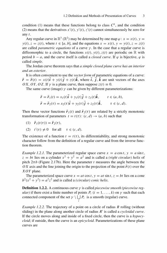
Example 1.2.2. The trajectory of a point on a circle of radius R rolling (withoutsliding) in the plane along another circle of radius R′ is called a cycloidal curve.If the circle moves along and inside of a fixed circle, then the curve is a hypocy-cloid; if outside, then the curve is an epicycloid. Parameterizations of these planecurves are
4 1. Theory of Curves in Three-dimensional Euclidean Space and in the Plane
x = R(m + 1) cos(mt) − Rm cos(mt + t),
y = R(m + 1) sin(mt) − Rm sin(mt + t) (1.1)
where m = R/R′ is the modulus. For m > 0 we have epicycloids, for m < 0,hypocycloids.
All cycloidal curves are piecewise regular. They are closed (periodic) for mrational only. A cardioid is an epicycloid with modulus m = 1; it has one sin-gular point. An astroid is a hypocycloid with modulus m = − 1
4 , see also Exer-cise 1.12.19. It has four singular points.
(a) cardioid (b) astroid
Figure 1.1. Cycloidal curves.
Besides the parametric presentation of a curve γ in R3 (R2) there also existother presentations.
Explicitly given curve. A particular case of the parametric presentation of acurve is an explicit presentation of a curve, when the part of a parameter t isplayed by either the variable x , y, or z; i.e., either x = x , y = f1(x), z =f2(x); x = f1(y), y = y, z = f2(y); or x = f1(z), y = f2(z), z = z.An explicit presentation is especially convenient for a plane curve. In this case acurve coincides with a graph of some function f , and then the equation of thecurve may be written either in the form y = f (x) or x = f (y).
Example 1.2.3. A tractrix (see Figure 2.12 a) can be presented as a graph x =a ln
a−√
a2−y2
y + √a2 − y2, 0 < y ≤ a. It has one singular point P(a, 0). For a
parameterization of this plane curve see Exercise 1.12.22.
Implicitly given curve. Let a differentiable map be given by
f : R3 → R2, f = [ f1(x, y, z), f2(x, y, z)].Then from the implicit function theorem it follows that if (0, 0) is a regular valueof the map f, then each connected component of the set T = f−1(0, 0) is a smooth
1.2 Definition and Methods of Presentation of Curves 5
regular curve in R3. In other words, under the above given conditions a set ofpoints in R3 whose coordinates satisfy the system of equations
f1(x, y, z) = 0, f2(x, y, z) = 0, (1.2)
forms a smooth regular curve (more exactly, a finite number of smooth regularcurves). This method is called an implicit presentation of a curve, and the system(1.2) is called the implicit equations of a curve. In the plane case, an implicitpresentation of a curve is based on a function f : R2 → R with the property that0 is a regular value.
Recall that the value (0, 0) of a map f = ( f1, f2) : R3 → R2 is regular if therank of the Jacobi matrix
J =(
∂ f1
∂x∂ f1
∂y∂ f1
∂z∂ f2
∂x∂ f2
∂y∂ f2
∂z
)is 2 (or det J �= 0) at every point of the solution set of (1.2) .
Obviously, an explicit presentation of a curve is at the same time a paramet-ric presentation, where the role of a parameter t is played by the x-coordinate,say. Conversely, if a regular curve is given by parametric equations, then in someneighborhood of an arbitrary point, as follows from the converse function the-orem, there an its explicit presentation. Analogously, if a curve is presented byimplicit equations, then in some neighborhood of an arbitrary point it admits anexplicit presentation. The last statement can be deduced from the implicit functiontheorem.
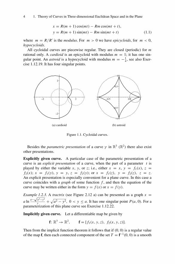
Example 1.2.4. (a) The intersection of a sphere x2 + y2 + z2 = R2 of radius Rwith a cylinder x2 + y2 = Rx of radius R
2 is a Viviani curve with one point of
00.20.61–0.4 0 0.4
–1
–0.5
0
0.5
1
(a) curve
–1–0.5
00.5
1
–1–0.5
00.5
–1
–0.5
0
0.5
1
(b) cylinder⋂
sphere
Figure 1.2. Viviani window.
self-intersection. One can verify that �r = [R cos2 t, R cos t sin t, R sin t], 0 ≤t ≤ 2π , is a regular parameterization of the curve.

6 1. Theory of Curves in Three-dimensional Euclidean Space and in the Plane
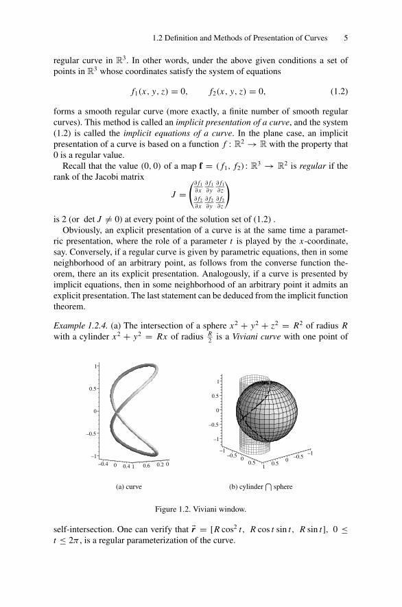
(b) The intersection of two cylinders with orthogonal axes, x2 + z2 = R21 and
y2 + z2 = R22, of radii R1 ≥ R2 is a bicylinder curve. One can verify that for
R1 = R2 it degenerates to a pair of ellipses, and that
�r =[
R1 cos t, ±√
R21 − R2
2 sin2 t, R1 sin t], 0 ≤ t ≤ 2π,
is a regular parameterization of the two curve components.
(a) curve (b) cylinder⋂
cylinder
Figure 1.3. Bicylinder curve.
1.3 Tangent Line and Osculating Plane
Let a smooth curve γ be given by the parametric equations
�r = �r(t) = x(t)�i + y(t)�j + z(t)�k.
The velocity vector of �r(t) at t = t0 is the derivative �r ′(t0) = x ′(t0)�i + y′(t0)�j +
z′(t0)�k. The velocity vector field is the vector function �r ′(t). The speed of �r(t) at
t = t0 is the length |�r ′(t0)| of the velocity vector.
Definition 1.3.1. The tangent line to a smooth curve γ at the point P = �r(t0) isthe straight line through the point P = �r(t0) ∈ γ in the direction of the velocityvector �r ′
(t0).
One can easily deduce the equations of a tangent line directly from its defi-nition. In the case of parametric equations of a curve we obtain �r = �R(u) =�r(t0) + u�r ′
(t0), or in detail, ⎧⎨⎩x = x(t0) + ux ′(t0),y = y(t0) + uy′(t0),z = z(t0) + uz′(t0),
(1.3)
1.3 Tangent Line and Osculating Plane 7
or in canonical form,
x − x(t0)
x ′(t0)= y − y(t0)
y′(t0)= z − z(t0)
z′(t0). (1.4)
In the case of explicit equations of a curve, y = ϕ1(x), z = ϕ2(x), the tangentline is given by the following equations:
x − x0 = y − ϕ1(x0)
ϕ′1(x0)
= z − ϕ2(x0)
ϕ′2(x0)
. (1.5)
Finally, if a curve γ is given by implicit equations
f1(x, y, z) = 0, f2(x, y, z) = 0,
and P(x0, y0, z0) belongs to γ , then the rank of the Jacobi matrix
J =(
∂ f1
∂x∂ f1
∂y∂ f1
∂z∂ f2
∂x∂ f2
∂y∂ f2
∂z
)
is 2 at P (i.e., rows and columns of J are each linearly independent). Assume fordefiniteness that the determinant ∣∣∣∣∣
∂ f1
∂x∂ f1
∂y∂ f2
∂x∂ f2
∂y
∣∣∣∣∣is nonzero. Then by the implicit function theorem there exist a real number ε > 0and differentiable functions ϕ1(x), ϕ2(y) such that for |x − x0| < ε,
f1(x, ϕ1(x), ϕ2(x)) ≡ 0, f2(x, ϕ1(x), ϕ2(x)) ≡ 0.
Hence the equations of a tangent line to a curve γ at the point P(x0, y0, z0) arepresented by (1.5), where the numbers ϕ′
1(x0) and ϕ′2(x0) are solutions of the
system of equations⎧⎨⎩∂ f1
∂x + ∂ f1
∂y · ϕ′1(x0) + ∂ f1
∂z · ϕ′2(x0) = 0,
∂ f2
∂x + ∂ f2
∂y · ϕ′1(x0) + ∂ f2
∂z · ϕ′2(x0) = 0.
(1.6)
In the case of an implicit presentation of a plane curve γ : f (x, y) = 0, the equa-tion of its tangent line can be written in the form
(∂ f /∂x)(x0, y0)(x − x0) + (∂ f /∂y)(x0, y0)(y − y0) = 0. (1.7)
1.3.1 Geometric Characterization of a Tangent Line
Denote by d the length of a chord of a curve joining the points P = γ (t0) andP1 = γ (t1), and by h the length of a perpendicular dropped from P1 onto thetangent line to γ at the point P .

8 1. Theory of Curves in Three-dimensional Euclidean Space and in the Plane
Theorem 1.3.1. limd→0
h
d= lim
t1→t0
h
d= 0.
Proof. From the definition of magnitudes d and h one may deduce their expres-sions
d = |�r(t1) − �r(t0)|, h = |�r ′(t0) × (�r(t1) − �r(t0))|
|�r ′(t0)| .
Then
limd→0
h
d= lim
t1→t0
|�r ′(t0) × (�r(t1) − �r(t0)|
|�r ′(t0)| · |�r(t1) − �r(t0)|
= limt1→t0
|�r ′(t0) × �r(t1)−�r(t0)
t1−t0|
|�r ′(t0)| · | �r(t1)−�r(t0)
t1−t0| = |�r ′
(t1) × �r ′(t0)|
|�r ′(t0)|2 = 0. �
Theorem 1.3.1 explains the geometric characterization of a tangent line.First of all, the theorem shows us that the tangent line l to a curve γ at the
point P = γ (t0) is the limit of secants to γ that pass through P and an arbitrarypoint P1 = γ (t1) for t1 → t0. In fact, if we denote by α an angle between l anda secant P P1, then h
d = sin α, and from Theorem 1.3.1 it follows that sin α → 0for t1 → t0. From this our statement follows.
Secondly, Theorem 1.3.1 estimates an error that we obtain from replacing acurve γ by its tangent line l. Let BP(d) = {x ∈ R3 : |x − P| < d} be a ballwith center P and radius d . Replace an arc γ
⋂BP(d) of a curve γ by the line
segment of l that belongs to BP(d). Then Theorem 1.3.1 claims that under sucha change we make an error of higher order than the radius d of a ball. Also, thistheorem allows us to give a geometric definition of a tangent line to a curve.
Denote by �τ (t0) a unit vector that is parallel to �r ′(t0) : �τ (t0) = �r ′
(t0)|�r ′
(t0)| . A straightline through the point P = γ (t0) that is orthogonal to the tangent line is called anormal line.
1.3.2 Osculating Plane
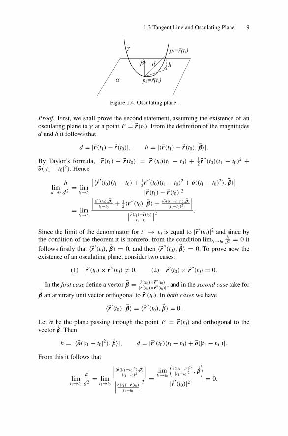
It is convenient to give a geometric definition of the osculating plane. Let a planeα with a unit normal �β pass through a point P = �r(t0) of a curve γ . Denote by dthe length of the chord of γ joining the points P0 = �r(t0) and P1 = �r(t1), and byh the length of the perpendicular dropped from P1 onto the plane α.
Definition 1.3.2. A plane α is called an osculating plane to a curve γ at a pointP = �r(t0) if
limd→0
h
d2= lim
t1→t0
h
d2= 0.
Theorem 1.3.2. At each point P = �r(t0) of a regular curve γ of class Ck (k ≥ 2)
there is an osculating plane α, and the vectors �r ′(t0) and �r ′′
(t0) are orthogonal toits normal vector �β.
1.3 Tangent Line and Osculating Plane 9
Figure 1.4. Osculating plane.
Proof. First, we shall prove the second statement, assuming the existence of anosculating plane to γ at a point P = �r(t0). From the definition of the magnitudesd and h it follows that
d = |�r(t1) − �r(t0)|, h = |〈�r(t1) − �r(t0), �β〉|.By Taylor’s formula, �r(t1) − �r(t0) = �r ′
(t0)(t1 − t0) + 12 �r ′′
(t0)(t1 − t0)2 +�o(|t1 − t0|2). Hence
limd→0
h
d2= lim
t1→t0
∣∣〈�r ′(t0)(t1 − t0) + 1
2 �r ′′(t0)(t1 − t0)2 + �o((t1 − t0)2), �β〉∣∣
|�r(t1) − �r(t0)|2
= limt1→t0
∣∣∣ 〈�r ′(t0),�β〉
t1−t0+ 1
2 〈�r ′′(t0), �β〉 + 〈�o(|t1−t0|2),�β〉
(t1−t0)2
∣∣∣∣∣ �r(t1)−�r(t0)t1−t0
∣∣2 .
Since the limit of the denominator for t1 → t0 is equal to |�r ′(t0)|2 and since by
the condition of the theorem it is nonzero, from the condition limt1→t0hd2 = 0 it
follows firstly that 〈�r ′(t0), �β〉 = 0, and then 〈�r ′′
(t0), �β〉 = 0. To prove now theexistence of an osculating plane, consider two cases:
(1) �r ′(t0) × �r ′′
(t0) �= 0, (2) �r ′(t0) × �r ′′
(t0) = 0.
In the first case define a vector �β = �r ′(t0)×�r ′′
(t0)|�r ′
(t0)×�r ′′(t0)| , and in the second case take for
�β an arbitrary unit vector orthogonal to �r ′(t0). In both cases we have
〈�r ′(t0), �β〉 = 〈�r ′′
(t0), �β〉 = 0.
Let α be the plane passing through the point P = �r(t0) and orthogonal to thevector �β. Then
h = |〈�o(|t1 − t0|2), �β〉|, d = |�r ′(t0)(t1 − t0) + �o(|t1 − t0|)|.
From this it follows that
limt1→t0
h
d2= lim
t1→t0
∣∣∣ 〈�o(|t1−t0|2),�β〉(t1−t0)2
∣∣∣∣∣∣ �r(t1)−�r(t0)t1−t0
∣∣∣2 =lim
t1→t0
⟨�o(|t1−t0|2)|t1−t0|2 , �β
⟩|�r ′
(t0)|2 = 0.
10 1. Theory of Curves in Three-dimensional Euclidean Space and in the Plane
Consequently, α is an osculating plane. Besides, as we see, in the first case theosculating plane is unique, and in the second case any plane containing a tangentline to γ at P = �r(t0) is an osculating plane. For a plane curve, the osculatingplane is the plane containing ϕ. �
We now deduce the equation of the osculating plane for the case that a curveis given by parametric equations and the vectors �r ′
(t0) and �r ′′(t0) at a given point
P = �r(t0) are linearly independent. In this case the normal vector to the osculatingplane, �β, as follows from Theorem 1.3.2, may be taken as �r ′
(t0) × �r ′′(t0),
�β = (y′ z′′ − y′′ z′)(t0)�i + (z′ x ′′ − z′′ x ′)(t0)�j + (x ′ y′′ − x ′′ y′)(t0)�k,
and we obtain the equation of an osculating plane α:
A(x − x(t0)) + B(y − y(t0)) + C(z − z(t0)) = 0,
where A = y′z′′ − y′′z′, B = z′x ′′ −z′′x ′, C = x ′y′′ −x ′′y′ are derived for t = t0.Projecting γ orthogonally onto an osculating plane α, we obtain a plane curve γ
of “minimal deviation” from γ . The value of this deviation has order slightly morethan d2. In detail, the lengths of the curves γ and γ that belong to the ball BP(d)
(with center P and radius d) differ from each other by a value whose order isslightly greater than d2.
At a point P = �r(t) of a curve, where an osculating plane is unique, one mayselect among all normal directions a unique normal vector �ν by the conditions
(1) �ν is orthogonal to �r ′(t0),
(2) �ν is parallel to an osculating plane,
(3) �ν forms an acute angle with the vector �r ′′(t0),
(4) �ν has unit length: |�ν| = 1.
Such a vector �ν is the principal normal vector to a curve γ at a point P . It iseasy to see that �ν can be expressed by the formula
�ν = − 〈�r ′, �r ′′〉
|�r ′| · |�r ′ × �r ′′| · �r ′ + |�r ′||�r ′ × �r ′′| · �r ′′
. (1.8)
A principal normal vector �ν is defined invariantly in the sense that its directiondoes not depend on the choice of a curve γ parameterization. Let �r = �R(τ ) beanother parameterization of γ . Then, as we know, there is a function t = t (τ )
such that �r(t (τ )) = �R(τ ) and
�R′τ = �r ′
t · t ′, �R′′ττ = �r ′′
t t · (t ′)2 + �r ′t · t ′′.
From these formulas it follows that 〈�ν, �R′τ 〉 = 0 and 〈�ν, �R′′
ττ 〉 = 〈�ν, �r ′′t t 〉 · (t ′)2,
and consequently, the vector �ν satisfies all four conditions with respect to theparameterization �R(τ ). Using the vectors �τ = �r ′
|�r ′| and �ν, define a vector �β by

1.4 Length of a Curve 11
the formula �β = �τ × �ν, and call it a binormal vector. The directions of �τ and �βdepend on the orientation of the curve and should be replaced by their oppositeswhen the orientation is reversed. The vector �ν, as was shown before, does notdepend on the orientation of the curve.
In practice, it is convenient to derive �τ , �ν, and �β in the following order: first,the vector �τ = �r ′
|�r ′| , then the vector �β = �r ′×�r ′′|�r ′×�r ′′| , and finally the vector �ν = �β × �τ .
Figure 1.5. Tangent, principal normal, and binormal vectors.
1.4 Length of a Curve
Let γ be a closed arc of some curve, and �r = �r(t) its parameterization; a ≤ t ≤ b.Note that a polygonal line is a curve in R3 (R2) composed of line segments pass-ing through adjacent points of some ordered finite set of points P1, P2, . . . , Pk . Apolygonal line σ is a regularly inscribed polygon in a curve γ if there is a partitionT of a line segment [a, b] by the points t1 < t2 < · · · < tk such that �O Pi = �r(ti ).To each polygonal line there corresponds its length l(σ ) equal to
∑k−1i=1 Pi Pi+1.
Denote by �(γ ) the set of all regularly inscribed polygonal lines in a curve γ .
Figure 1.6. Regularly inscribed polygonal lines in a curve.
Definition 1.4.1. A continuous curve γ is called rectifiable if supσ∈�(γ ) l(σ ) <
∞.
Definition 1.4.2. The length of a rectifiable curve γ is defined as the least up-per bound of lengths of all regularly inscribed polygonal lines in a given curveγ : l(γ ) = supσ∈�(γ ) l(σ ).
12 1. Theory of Curves in Three-dimensional Euclidean Space and in the Plane
The next theorem gives us a sufficient condition for the existence of the lengthof a curve and the formula to calculate it.
Theorem 1.4.1. A closed arc of any smooth curve is rectifiable, and its length is
l(γ ) =∫ b
a|�r ′
(t)| dt.
Proof. Let �r = �r(t) = x(t)�i + y(t)�j + z(t)�k (t ∈ [a, b]) be a smooth param-eterization of a closed arc γ of a given curve. Take an arbitrary polygonal lineσ : P1, P2, . . . , Pk from the set �(γ ). The length of the i th segment of the polyg-onal line σ is equal to
Pi Pi+1 = |�r(ti+1) − �r(ti )|=√
[x(ti+1) − x(ti )]2 + [y(ti+1) − y(ti )]2 + [z(ti+1) − z(ti )]2.
Applying Lagrange’s formula to each of the functions x(t), y(t) and z(t), weobtain
Pi Pi+1 =√
[x ′(ξi )]2 + [y′(ηi )]2 + [z′(si )]2 �ti , (1.9)
where ti ≤ ξi ≤ ti+1, ti ≤ ηi ≤ ti+1, ti ≤ si ≤ ti+1, �ti = ti+1 − ti . Sincethe functions x ′(t), y′(t) and z′(t) are continuous on a closed interval [a, b], byWeierstrass’s first theorem they are bounded on this closed interval; i.e., there isa real M such that |x ′(t)| < M, |y′(t)| < M , and |z′(t)| < M , for all t ∈ [a, b].Using the last inequality we obtain
l(σ ) =∑k−1
i=1Pi Pi+1 ≤ √
3M∑k−1
i=1�ti = √
3M(b − a).
Since σ is an arbitrary polygonal line from the set �(γ ), it follows that
supσ∈�(γ )
l(σ ) ≤ √3M(b − a) < ∞.
The proof of the first statement of the theorem is complete.Now we shall prove the second statement of the theorem.To each polygonal line σ : P1, P2, . . . , Pk regularly inscribed in γ there corre-
sponds some partitionT (σ ) : t1 < t2 < · · · < tk
of a closed interval [a, b], and conversely, to each partition T : t1 < t2 < · · · < tkof a closed interval [a, b] there corresponds a polygonal line σ(T ) : P1, P2, . . . ,Pk , where Pi is the endpoint of the vector �r(ti ). For each polygonal line σ(t)define a number δ(T ) = maxi=1...k−1 �ti . We now prove that for any real ε > 0there is a partition T : t1 < t2 < · · · < tk of the line segment [a, b] for which thefollowing inequalities hold simultaneously:
1.4 Length of a Curve 13
|l(γ ) − l(σ (T ))| ≤ ε
3, (1.10)∣∣∣l(σ (T )) −
∑k−1
i=1|�r ′
(ti )|�ti∣∣∣ ≤ ε
3, (1.11)∣∣∣∣∑k−1
i=1|�r ′
(t0)|�ti −∫ b
a|�r ′
(t)|dt
∣∣∣∣ ≤ ε
3. (1.12)
Directly from the definition of the length of the curve γ and that it is rectifiablefollows the existence of a partition T1 of the line segment [a, b] such that inequal-ity (1.10) holds. The sum ∑k−1
i=1|�r ′
(ti )|�ti
is a Riemann integral sum for the integral∫ b
a |�r ′(t)|dt. Thus there is a real number
δ0 > 0 such that for every partition T of a line segment [a, b] with the propertyδ(T ) < δ0, the inequality (1.12) holds. Now take a partition T2 of the line segment[a, b] refining the partition T1 and satisfying the inequality (1.12). For the partitionT2, in view of the triangle inequality, the inequalities (1.10) and (1.12) hold. Thefunctions x ′(t), y′(t), and z′(t) are continuous and hence uniformly continuouson [a, b]. Thus for any real ε1 > 0 there is a real number δ1 > 0 such that for|t ′′ − t ′| < δ1, the inequalities
|x ′(t ′′) − x ′(t ′)| < ε1, |y′(t ′′) − y′(t ′)| < ε1, |z′(t ′′) − z′(t ′)| < ε1
hold. Now take a partition T3 of the line segment [a, b] refining the partition T2
and satisfying the inequality δ(T3) ≤ min{δ0, δ1}. For the i th segment Pi Pi+1 ofsuch a partition we have∣∣Pi Pi+1 − |�r ′
(ti )| · �ti∣∣
=∣∣∣√[x ′(ξi )]2 + [y′(ηi )]2 + [z′(ζi )]2 −
√[x ′(ti )]2 + [y′(ti )]2 + [z′(ti )]2
∣∣∣�ti
≤√
[x ′(ξi ) − x ′(ti )]2 + [y′(ηi ) − y′(ti )]2 + [z′(ζi ) − z′(ti )]2�ti ≤ √3ε1�ti ,
where the next-to-last inequality holds in view of the triangle inequality. Summingup these inequalities, we obtain∣∣∣l(σ (T3)) −
∑n(T3)−1
i=1|�r ′
(ti )|�ti )∣∣∣ ≤ √
3ε1(b − a),
where n(T3) is the number of segments of the partition T3. Select ε1 satisfying theinequality
√3ε1(b − a) < ε
3 . Thus, if we take the partition T3 in the role of thepartition T of the line segment [a, b], then the inequalities (1.10)–(1.12) will besatisfied simultaneously. Thus, summing up these inequalities, we obtain∣∣∣∣l(γ ) −
∫ b
a|�r ′
(t)| dt
∣∣∣∣ ≤ ε
3+ ε
3+ ε
3= ε. (1.13)
Since ε > 0 is an arbitrary real number, the proof of second part of the theoremis complete. �
14 1. Theory of Curves in Three-dimensional Euclidean Space and in the Plane
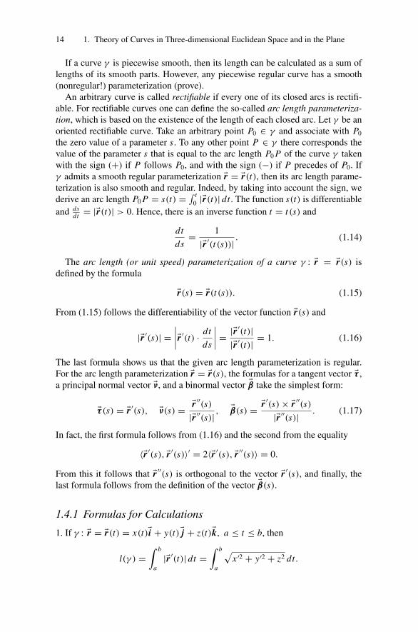
If a curve γ is piecewise smooth, then its length can be calculated as a sum oflengths of its smooth parts. However, any piecewise regular curve has a smooth(nonregular!) parameterization (prove).
An arbitrary curve is called rectifiable if every one of its closed arcs is rectifi-able. For rectifiable curves one can define the so-called arc length parameteriza-tion, which is based on the existence of the length of each closed arc. Let γ be anoriented rectifiable curve. Take an arbitrary point P0 ∈ γ and associate with P0
the zero value of a parameter s. To any other point P ∈ γ there corresponds thevalue of the parameter s that is equal to the arc length P0 P of the curve γ takenwith the sign (+) if P follows P0, and with the sign (−) if P precedes of P0. Ifγ admits a smooth regular parameterization �r = �r(t), then its arc length parame-terization is also smooth and regular. Indeed, by taking into account the sign, wederive an arc length P0 P = s(t) = ∫ t
0 |�r(t)| dt . The function s(t) is differentiableand ds
dt = |�r(t)| > 0. Hence, there is an inverse function t = t (s) and
dt
ds= 1
|�r ′(t (s))| . (1.14)
The arc length (or unit speed) parameterization of a curve γ : �r = �r(s) isdefined by the formula
�r(s) = �r(t (s)). (1.15)
From (1.15) follows the differentiability of the vector function �r(s) and
|�r ′(s)| =
∣∣∣∣�r ′(t) · dt
ds
∣∣∣∣ = |�r ′(t)|
|�r ′(t)| = 1. (1.16)
The last formula shows us that the given arc length parameterization is regular.For the arc length parameterization �r = �r(s), the formulas for a tangent vector �τ ,a principal normal vector �ν, and a binormal vector �β take the simplest form:
�τ (s) = �r ′(s), �ν(s) = �r ′′
(s)
|�r ′′(s)| ,
�β(s) = �r ′(s) × �r ′′
(s)
|�r ′′(s)| . (1.17)
In fact, the first formula follows from (1.16) and the second from the equality
〈�r ′(s), �r ′
(s)〉′ = 2〈�r ′(s), �r ′′
(s)〉 = 0.
From this it follows that �r ′′(s) is orthogonal to the vector �r ′
(s), and finally, thelast formula follows from the definition of the vector �β(s).
1.4.1 Formulas for Calculations
1. If γ : �r = �r(t) = x(t)�i + y(t)�j + z(t)�k, a ≤ t ≤ b, then
l(γ ) =∫ b
a|�r ′
(t)| dt =∫ b
a
√x ′2 + y′2 + z2 dt.
1.5 Problems: Convex Plane Curves 15
2. If γ : y = f1(x), z = f2(x), a ≤ x ≤ b, then
l(γ ) =∫ b
a
√1 + f ′
12 + f ′
22 dx .
3. If γ (t) : �r = �r(t) = x(t)�i + y(t)�j , a plane curve, then
l(γ ) =∫ b
a
√x ′2 + y′2 dt. (1.18)
4. If γ : y = f (x), a ≤ x ≤ b, then
l(γ ) =∫ b
a
√1 + f ′2 dx .
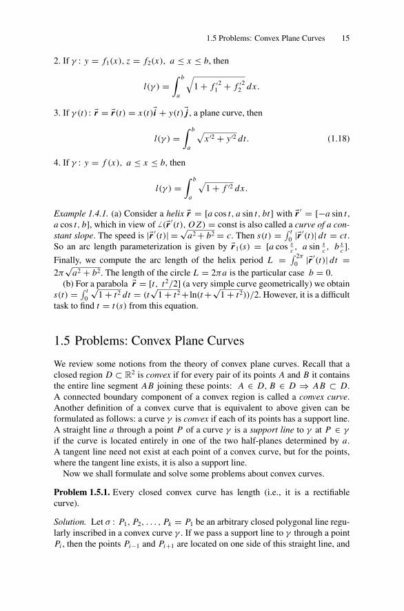
Example 1.4.1. (a) Consider a helix �r = [a cos t, a sin t, bt] with �r ′ = [−a sin t ,a cos t, b], which in view of � (�r ′
(t), O Z) = const is also called a curve of a con-stant slope. The speed is |�r ′
(t)| = √a2 + b2 = c. Then s(t) = ∫ t
0 |�r ′(t)| dt = ct .
So an arc length parameterization is given by �r1(s) = [a cos sc , a sin s
c , b sc ].
Finally, we compute the arc length of the helix period L = ∫ 2π
0 |�r ′(t)| dt =
2π√
a2 + b2. The length of the circle L = 2πa is the particular case b = 0.(b) For a parabola �r = [t, t2/2] (a very simple curve geometrically) we obtain
s(t) = ∫ t0
√1 + t2 dt = (t
√1 + t2 + ln(t +√
1 + t2))/2. However, it is a difficulttask to find t = t (s) from this equation.
1.5 Problems: Convex Plane Curves
We review some notions from the theory of convex plane curves. Recall that aclosed region D ⊂ R2 is convex if for every pair of its points A and B it containsthe entire line segment AB joining these points: A ∈ D, B ∈ D ⇒ AB ⊂ D.A connected boundary component of a convex region is called a convex curve.Another definition of a convex curve that is equivalent to above given can beformulated as follows: a curve γ is convex if each of its points has a support line.A straight line a through a point P of a curve γ is a support line to γ at P ∈ γ
if the curve is located entirely in one of the two half-planes determined by a.A tangent line need not exist at each point of a convex curve, but for the points,where the tangent line exists, it is also a support line.
Now we shall formulate and solve some problems about convex curves.
Problem 1.5.1. Every closed convex curve has length (i.e., it is a rectifiablecurve).
Solution. Let σ : P1, P2, . . . , Pk = P1 be an arbitrary closed polygonal line regu-larly inscribed in a convex curve γ . If we pass a support line to γ through a pointPi , then the points Pi−1 and Pi+1 are located on one side of this straight line, and
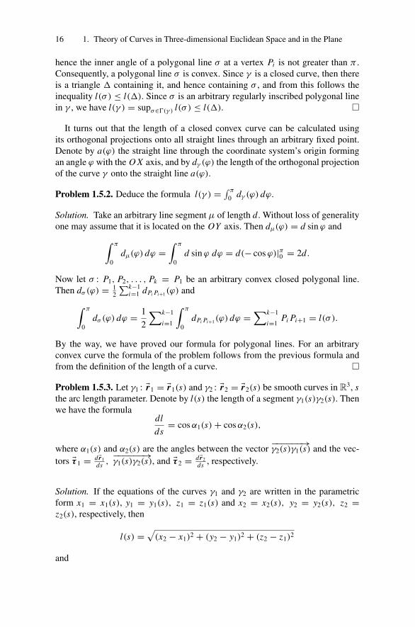
16 1. Theory of Curves in Three-dimensional Euclidean Space and in the Plane
hence the inner angle of a polygonal line σ at a vertex Pi is not greater than π .Consequently, a polygonal line σ is convex. Since γ is a closed curve, then thereis a triangle � containing it, and hence containing σ , and from this follows theinequality l(σ ) ≤ l(�). Since σ is an arbitrary regularly inscribed polygonal linein γ , we have l(γ ) = supσ∈�(γ ) l(σ ) ≤ l(�). �
It turns out that the length of a closed convex curve can be calculated usingits orthogonal projections onto all straight lines through an arbitrary fixed point.Denote by a(ϕ) the straight line through the coordinate system’s origin formingan angle ϕ with the O X axis, and by dγ (ϕ) the length of the orthogonal projectionof the curve γ onto the straight line a(ϕ).
Problem 1.5.2. Deduce the formula l(γ ) = ∫ π
0 dγ (ϕ) dϕ.
Solution. Take an arbitrary line segment µ of length d . Without loss of generalityone may assume that it is located on the OY axis. Then dµ(ϕ) = d sin ϕ and∫ π
0dµ(ϕ) dϕ =
∫ π
0d sin ϕ dϕ = d(− cos ϕ)|π0 = 2d.
Now let σ : P1, P2, . . . , Pk = P1 be an arbitrary convex closed polygonal line.Then dσ (ϕ) = 1
2
∑k−1i=1 dPi Pi+1(ϕ) and∫ π
0dσ (ϕ) dϕ = 1
2
∑k−1
i=1
∫ π
0dPi Pi+1(ϕ) dϕ =
∑k−1
i=1Pi Pi+1 = l(σ ).
By the way, we have proved our formula for polygonal lines. For an arbitraryconvex curve the formula of the problem follows from the previous formula andfrom the definition of the length of a curve. �
Problem 1.5.3. Let γ1 : �r1 = �r1(s) and γ2 : �r2 = �r2(s) be smooth curves in R3, sthe arc length parameter. Denote by l(s) the length of a segment γ1(s)γ2(s). Thenwe have the formula
dl
ds= cos α1(s) + cos α2(s),
where α1(s) and α2(s) are the angles between the vector−−−−−−→γ2(s)γ1(s) and the vec-
tors �τ 1 = d�r1ds ,
−−−−−−→γ1(s)γ2(s), and �τ 2 = d�r2
ds , respectively.
Solution. If the equations of the curves γ1 and γ2 are written in the parametricform x1 = x1(s), y1 = y1(s), z1 = z1(s) and x2 = x2(s), y2 = y2(s), z2 =z2(s), respectively, then
l(s) =√
(x2 − x1)2 + (y2 − y1)2 + (z2 − z1)2
and

1.5 Problems: Convex Plane Curves 17
Figure 1.7. First variation of the distance l(s) = |γ1(s)γ2(s)|.
dl
ds= (x2 − x1)(x ′
2 − x ′1) + (y2 − y1)(y′
2 − y′1) + (z2 − z1)(z′
2 − z′1)√
(x2 − x1)2 + (y2 − y1)2 + (z2 − z1)2
= (x1 − x2)x ′1 + (y1 − y2)y′
1 + (z1 − z2)z′1
l(s)
+ (x2 − x1)x ′2 + (y2 − y1)y′
2 + (z2 − z1)z′2
l(s)
=⟨ −−→γ2γ1
|γ2γ1| , �τ 1
⟩+⟨ −−→γ1γ2
|γ1γ2| , �τ 2
⟩= cos α1(s) + cos α2(s).
In the particular case that γ2 degenerates to a point, we have dlds = cos α1(s). If
the curves γ1 and γ2 are parameterized by an arbitrary parameter t , and l(t) =γ1(t)γ2(t), then
dl
dt= cos α1(t)
ds1
dt+ cos α2(t)
ds2
dt,
where s1(t) = ∫ t0 |�r1(t)| dt and s2(t) = ∫ t
0 |�r2(t)| dt . �
Problem 1.5.4. Let γ be an arc of a smooth convex curve with endpoints A1 andA2. Denote by l(h) the length of a chord A1(h)A2(h) on γ that is parallel to thestraight line A1 A2 and is located at distance h from it. Denote by α1(h) and α2(h)
the angles that the chord A1(h)A2(h) forms with γ . Then the following formulaholds:
dl
dh= cot α1(h) + cot α2(h).
Figure 1.8. Derivative of the length of a chord A1(h)A2(h).
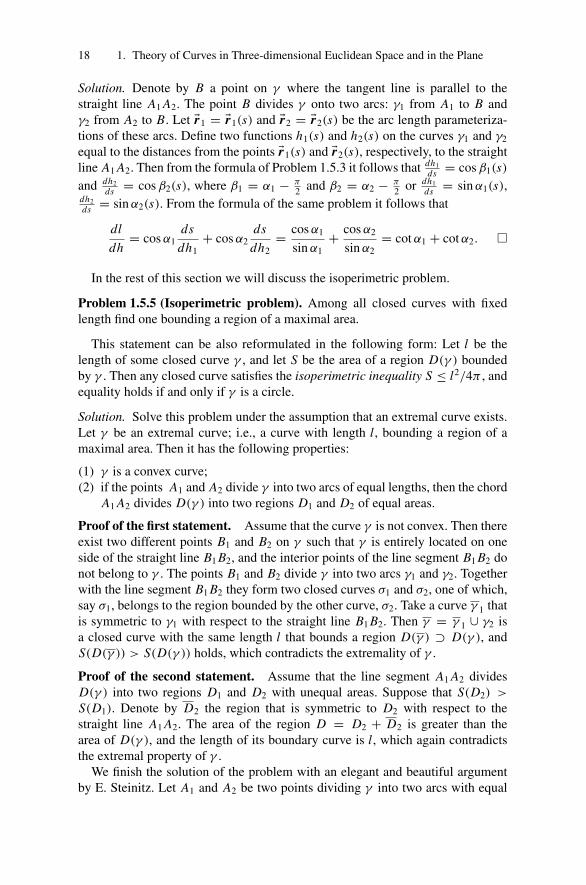
18 1. Theory of Curves in Three-dimensional Euclidean Space and in the Plane
Solution. Denote by B a point on γ where the tangent line is parallel to thestraight line A1 A2. The point B divides γ onto two arcs: γ1 from A1 to B andγ2 from A2 to B. Let �r1 = �r1(s) and �r2 = �r2(s) be the arc length parameteriza-tions of these arcs. Define two functions h1(s) and h2(s) on the curves γ1 and γ2
equal to the distances from the points �r1(s) and �r2(s), respectively, to the straightline A1 A2. Then from the formula of Problem 1.5.3 it follows that dh1
ds = cos β1(s)and dh2
ds = cos β2(s), where β1 = α1 − π2 and β2 = α2 − π
2 or dh1ds = sin α1(s),
dh2ds = sin α2(s). From the formula of the same problem it follows that
dl
dh= cos α1
ds
dh1+ cos α2
ds
dh2= cos α1
sin α1+ cos α2
sin α2= cot α1 + cot α2. �
In the rest of this section we will discuss the isoperimetric problem.
Problem 1.5.5 (Isoperimetric problem). Among all closed curves with fixedlength find one bounding a region of a maximal area.
This statement can be also reformulated in the following form: Let l be thelength of some closed curve γ , and let S be the area of a region D(γ ) boundedby γ . Then any closed curve satisfies the isoperimetric inequality S ≤ l2/4π , andequality holds if and only if γ is a circle.
Solution. Solve this problem under the assumption that an extremal curve exists.Let γ be an extremal curve; i.e., a curve with length l, bounding a region of amaximal area. Then it has the following properties:
(1) γ is a convex curve;(2) if the points A1 and A2 divide γ into two arcs of equal lengths, then the chord
A1 A2 divides D(γ ) into two regions D1 and D2 of equal areas.
Proof of the first statement. Assume that the curve γ is not convex. Then thereexist two different points B1 and B2 on γ such that γ is entirely located on oneside of the straight line B1 B2, and the interior points of the line segment B1 B2 donot belong to γ . The points B1 and B2 divide γ into two arcs γ1 and γ2. Togetherwith the line segment B1 B2 they form two closed curves σ1 and σ2, one of which,say σ1, belongs to the region bounded by the other curve, σ2. Take a curve γ 1 thatis symmetric to γ1 with respect to the straight line B1 B2. Then γ = γ 1 ∪ γ2 isa closed curve with the same length l that bounds a region D(γ ) ⊃ D(γ ), andS(D(γ )) > S(D(γ )) holds, which contradicts the extremality of γ .
Proof of the second statement. Assume that the line segment A1 A2 dividesD(γ ) into two regions D1 and D2 with unequal areas. Suppose that S(D2) >
S(D1). Denote by D2 the region that is symmetric to D2 with respect to thestraight line A1 A2. The area of the region D = D2 + D2 is greater than thearea of D(γ ), and the length of its boundary curve is l, which again contradictsthe extremal property of γ .
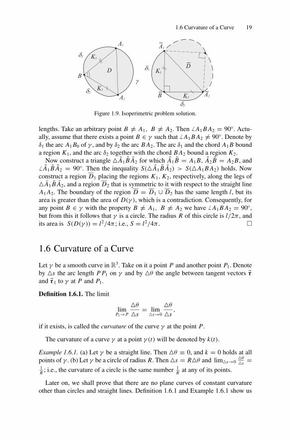
We finish the solution of the problem with an elegant and beautiful argumentby E. Steinitz. Let A1 and A2 be two points dividing γ into two arcs with equal
1.6 Curvature of a Curve 19
Figure 1.9. Isoperimetric problem solution.
lengths. Take an arbitrary point B �= A1, B �= A2. Then � A1 B A2 = 90◦. Actu-ally, assume that there exists a point B ∈ γ such that � A1 B A2 �= 90◦. Denote byδ1 the arc A1 B0 of γ , and by δ2 the arc B A2. The arc δ1 and the chord A1 B bounda region K1, and the arc δ2 together with the chord B A2 bound a region K2.
Now construct a triangle � A1 B A2 for which A1 B = A1 B, A2 B = A2 B, and� A1 B A2 = 90◦. Then the inequality S(� A1 B A2) > S(�A1 B A2) holds. Nowconstruct a region D1 placing the regions K1, K2, respectively, along the legs of� A1 B A2, and a region D2 that is symmetric to it with respect to the straight lineA1 A2. The boundary of the region D = D1 ∪ D2 has the same length l, but itsarea is greater than the area of D(γ ), which is a contradiction. Consequently, forany point B ∈ γ with the property B �= A1, B �= A2 we have � A1 B A2 = 90◦,but from this it follows that γ is a circle. The radius R of this circle is l/2π , andits area is S(D(γ )) = l2/4π ; i.e., S = l2/4π . �
1.6 Curvature of a Curve
Let γ be a smooth curve in R3. Take on it a point P and another point P1. Denoteby �s the arc length P P1 on γ and by �θ the angle between tangent vectors �τand �τ 1 to γ at P and P1.
Definition 1.6.1. The limit
limP1→P
�θ
�s= lim
�s→0
�θ
�s,
if it exists, is called the curvature of the curve γ at the point P .
The curvature of a curve γ at a point γ (t) will be denoted by k(t).
Example 1.6.1. (a) Let γ be a straight line. Then �θ ≡ 0, and k = 0 holds at allpoints of γ . (b) Let γ be a circle of radius R. Then �s = R�θ and lim�s→0
�θ
�s =1R ; i.e., the curvature of a circle is the same number 1
R at any of its points.
Later on, we shall prove that there are no plane curves of constant curvatureother than circles and straight lines. Definition 1.6.1 and Example 1.6.1 show us
20 1. Theory of Curves in Three-dimensional Euclidean Space and in the Plane
that the curvature of a curve is the measure of its deviation from a straight line ina neighborhood of a given point, and that the curvature is greater as this deviationis greater. The following theorem gives us sufficient conditions for the existenceof the curvature and a formula for its derivation.
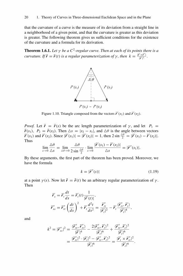
Theorem 1.6.1. Let γ be a C2-regular curve. Then at each of its points there is acurvature. If �r = �r(t) is a regular parameterization of γ , then k = |�r ′×�r ′′|
|�r ′|3 .
Figure 1.10. Triangle composed from the vectors �r ′(s1) and �r ′(s2).
Proof. Let �r = �r(s) be the arc length parameterization of γ , and let P1 =�r(s1), P2 = �r(s2). Then �s = |s2 − s1|, and �θ is the angle between vectors�r ′
(s1) and �r ′(s2). Since |�r ′
(s1)| = |�r ′(s2)| = 1, then 2 sin �θ
2 = |�r ′(s1) − �r ′
(s2)|.Thus
lims→0
�θ
�s= lim
�θ→0
�θ
2 sin �θ
2
· lims→0
|�r ′(s1) − �r ′
(s2)|�s
= |�r ′′(s1)|.
By these arguments, the first part of the theorem has been proved. Moreover, wehave the formula
k = |�r ′′(s)| (1.19)
at a point γ (s). Now let �r = �r(t) be an arbitrary regular parameterization of γ .Then
�r ′s = �r ′
t
dt
ds= �r ′
t (t)1
|�r ′(t)| ,
�r ′′ss = �r ′′
t t
(dt
ds
)2
+ �r ′t
d2t
ds2= �r ′′
t t
|�r ′t |2
− �r ′t
〈�r ′′t t , �r ′
t 〉|�r ′
t |4,
and
k2 = |�r ′′ss |2 = 〈�r ′′
t t , �r ′′t t 〉
|�r ′|4 − 2〈�r ′′t t , �r ′
t 〉2
|�r ′t |6
+ 〈�r ′′t t , �r ′
t 〉2
|�r ′t |6
= |�r ′′t t |2 · |�r ′
t |2 − 〈�r ′′t t , �r ′
t 〉2
|�r ′t |6
= |�r ′t × �r ′′
t t |2|�r ′
t |6.
1.6 Curvature of a Curve 21
From this follows
k = |�r ′′t t × �r ′
t ||�r ′
t |3. �
The last formula shows us that the noncollinearity condition of the vectors �r ′t
and �r ′′t t has a geometrical sense; i.e., it does not depend on the choice of a pa-
rameterization. If at some point of γ the curvature is nonzero, then �r ′t and �r ′′
t t arenonparallel and conversely.
This remark allows us to give a geometric condition for the uniqueness of theosculating plane to a curve γ at any of its points P , and to complete Theorem 1.3.2by the following statement.
Theorem 1.6.2. A necessary and sufficient condition for the existence of a uniqueosculating plane to a C2-regular curve γ at any of its points is that the curvatureof γ be nonzero at this point.
As we have just shown, a straight line has zero curvature at each of its points.The converse statement is also true: if the curvature of a curve γ at each of itspoint is zero, then γ is a straight line. Indeed, if k ≡ 0, then �r ′′
ss ≡ 0, from whichfollows �r ′
s = �c1 and �r = �c1s + �c2.
1.6.1 Formulas for Calculations
(1) If γ : �r = �r(t) = x(t)�i + y(t)�j + z(t)�k, then
k =√
(y′z′′ − z′y′′)2 + (z′x ′′ − x ′z′′)2 + (x ′y′′ − y′x ′′)2
(x ′2 + y′2 + z′2) 32
,
(2) If γ is a plane curve �r = �r(t) = x(t)�i + y(t)�j , then
k = |y′′x ′ − x ′′y′|(x ′2 + y′2) 3
2
,
(3) If γ is a graph y = f (x), then
k = | f ′′(x)|(1 + x ′2) 3
2
.
1.6.2 Plane Curves
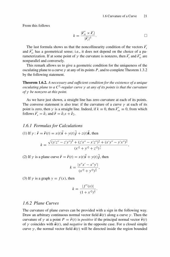
The curvature of plane curves can be provided with a sign in the following way.Draw an arbitrary continuous normal vector field �n(t) along a curve γ . Then thecurvature of γ at a point P = �r(t) is positive if the principal normal vector �ν(t)of γ coincides with �n(t), and negative in the opposite case. For a closed simplecurve γ , the normal vector field �n(t) will be directed inside the region bounded
22 1. Theory of Curves in Three-dimensional Euclidean Space and in the Plane
Figure 1.11. The plane curve sign of curvature.
by γ . In this case, the curvature of a curve γ is positive at a point if the region isconvex “outwards,” and the curvature is negative if it is convex “inwards.”
In particular, by this definition of a curvature’s sign, a closed convex curve hasnonnegative curvature at each point. For oriented curves denote by α(t) the anglebetween the vector �r ′
(t) and the direction of the O X axis, and define the cur-vature’s sign as the rate at which the angle α(t) is changing, where we assumesignk = sign dα
dt . The value of the angle α(t) is defined by the following method:
the angle α(0) is equal to the angle measured from �i counterclockwise with sign(+), or clockwise with sign (−). For other values of t the angle α(t) is definedby continuity; it increases when the vector �r ′
(t) turns counterclockwise, and de-creases otherwise.
In particular, if a plane curve γ is given explicitly as y = f (x), then it naturallyobtains an orientation (by increasing x-variable), and then the curvature’s signcoincides with the sign of f ′′(x); i.e., in this case, k = f ′′
(1+ f ′2)3/2 . If a curve is
given by the arc length parameterization, then k(s) = dαds . If the curvature k of a
curve at any of its points is nonzero, then the real number 1/|k| is called the radiusof curvature of the curve at the given point and is denoted by R : R = 1/|k|. Wesay that the radius of curvature is infinite if the curvature is zero; moreover, theradius of curvature R can be is considered with the sign in correspondence withthe formula R = 1/k.
Plane curves are uniquely determined by their curvature k(s), given as a func-tion of the arc length parameter s. But before we formulate this theorem, we shallgeneralize the definition of a curve given above.
Due to Definition 1.2.1, we represent a regular curve as the differentiable im-age of an open interval or a circle into R2 (or R3). Such a definition was suf-ficient for studying the local properties of a curve. However, when one studiesthe properties of a curve as a whole, inevitably there appear curves with points ofself-intersection. Moreover, curves defined by their geometrical properties also of-ten have points of self-intersection, for example, elongated cycloids and hypocy-cloids, lemniscates of Bernoulli, etc.
Thus, we shall hereinafter define a curve as a locally diffeomorphic image ofan open interval I or a circle S1 into R2 (or R3).
More precisely, two local diffeomorphisms ϕ1(t) and ϕ2(t) of an open intervalor a circle into R2 (or R3) are equivalent if there is a diffeomorphism t = t (τ ) ofan open interval or a circle onto itself such that ϕ1(t (τ )) ≡ ϕ2(t).
1.6 Curvature of a Curve 23
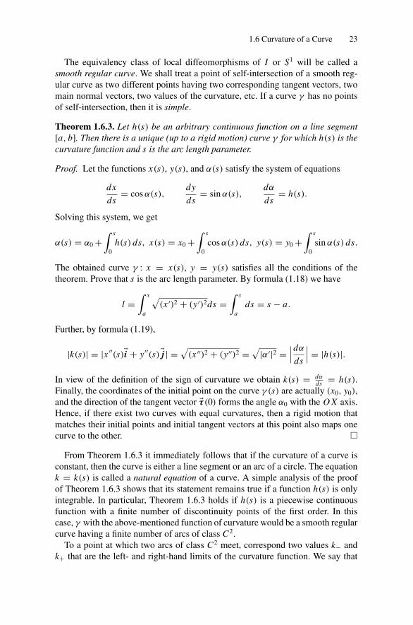
The equivalency class of local diffeomorphisms of I or S1 will be called asmooth regular curve. We shall treat a point of self-intersection of a smooth reg-ular curve as two different points having two corresponding tangent vectors, twomain normal vectors, two values of the curvature, etc. If a curve γ has no pointsof self-intersection, then it is simple.
Theorem 1.6.3. Let h(s) be an arbitrary continuous function on a line segment[a, b]. Then there is a unique (up to a rigid motion) curve γ for which h(s) is thecurvature function and s is the arc length parameter.
Proof. Let the functions x(s), y(s), and α(s) satisfy the system of equations
dx
ds= cos α(s),
dy
ds= sin α(s),
dα
ds= h(s).
Solving this system, we get
α(s) = α0 +∫ s
0h(s) ds, x(s) = x0 +
∫ s
0cos α(s) ds, y(s) = y0 +
∫ s
0sin α(s) ds.
The obtained curve γ : x = x(s), y = y(s) satisfies all the conditions of thetheorem. Prove that s is the arc length parameter. By formula (1.18) we have
l =∫ s
a
√(x ′)2 + (y′)2ds =
∫ s
ads = s − a.
Further, by formula (1.19),
|k(s)| = |x ′′(s)�i + y′′(s)�j | =√
(x ′′)2 + (y′′)2 =√
|α′|2 =∣∣∣dα
ds
∣∣∣ = |h(s)|.
In view of the definition of the sign of curvature we obtain k(s) = dαds = h(s).
Finally, the coordinates of the initial point on the curve γ (s) are actually (x0, y0),and the direction of the tangent vector �τ (0) forms the angle α0 with the O X axis.Hence, if there exist two curves with equal curvatures, then a rigid motion thatmatches their initial points and initial tangent vectors at this point also maps onecurve to the other. �
From Theorem 1.6.3 it immediately follows that if the curvature of a curve isconstant, then the curve is either a line segment or an arc of a circle. The equationk = k(s) is called a natural equation of a curve. A simple analysis of the proofof Theorem 1.6.3 shows that its statement remains true if a function h(s) is onlyintegrable. In particular, Theorem 1.6.3 holds if h(s) is a piecewise continuousfunction with a finite number of discontinuity points of the first order. In thiscase, γ with the above-mentioned function of curvature would be a smooth regularcurve having a finite number of arcs of class C2.
To a point at which two arcs of class C2 meet, correspond two values k− andk+ that are the left- and right-hand limits of the curvature function. We say that
24 1. Theory of Curves in Three-dimensional Euclidean Space and in the Plane
the curvature of a curve γ at this point is not smaller than k0 (not greater than k0)if min(k−, k+) ≥ k0 (max(k−, k+) ≤ k0).
In Section 1.7 if the opposite is not supposed, we shall refer to a curve γ fromthis class; i.e., a smooth regular curve with a piecewise continuous curvature func-tion k(s).
1.7 Problems: Curvature of Plane Curves
Let two plane curves γ1 and γ2 touch each other at a common point M , and let thecurvature sign of γ1 and γ2 be defined using the same normal vector �n. Denote byk1 and k2 the curvatures of the curves γ1 and γ2 at M .
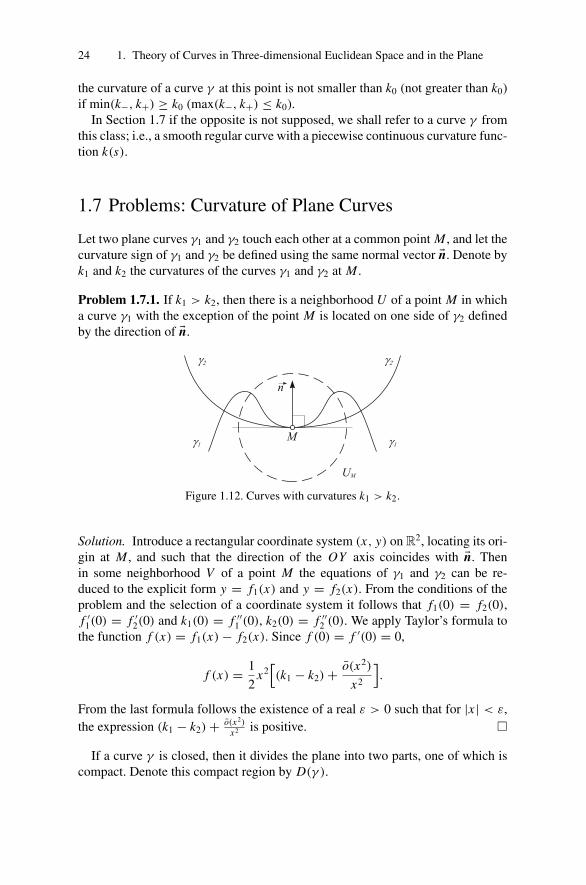
Problem 1.7.1. If k1 > k2, then there is a neighborhood U of a point M in whicha curve γ1 with the exception of the point M is located on one side of γ2 definedby the direction of �n.
Figure 1.12. Curves with curvatures k1 > k2.
Solution. Introduce a rectangular coordinate system (x, y) on R2, locating its ori-gin at M , and such that the direction of the OY axis coincides with �n. Thenin some neighborhood V of a point M the equations of γ1 and γ2 can be re-duced to the explicit form y = f1(x) and y = f2(x). From the conditions of theproblem and the selection of a coordinate system it follows that f1(0) = f2(0),f ′1(0) = f ′
2(0) and k1(0) = f ′′1 (0), k2(0) = f ′′
2 (0). We apply Taylor’s formula tothe function f (x) = f1(x) − f2(x). Since f (0) = f ′(0) = 0,
f (x) = 1
2x2[(k1 − k2) + o(x2)
x2
].
From the last formula follows the existence of a real ε > 0 such that for |x | < ε,the expression (k1 − k2) + o(x2)
x2 is positive. �
If a curve γ is closed, then it divides the plane into two parts, one of which iscompact. Denote this compact region by D(γ ).
1.7 Problems: Curvature of Plane Curves 25
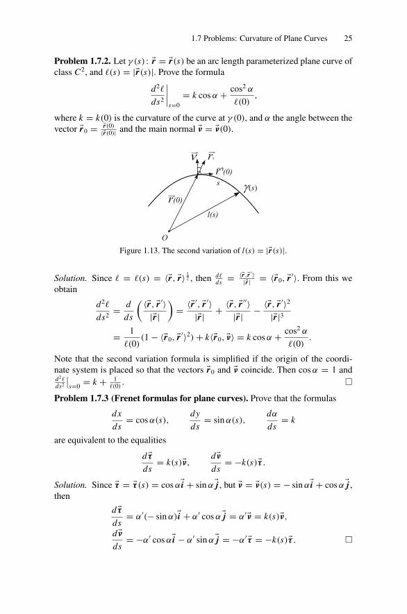
Problem 1.7.2. Let γ (s) : �r = �r(s) be an arc length parameterized plane curve ofclass C2, and �(s) = |�r(s)|. Prove the formula
d2�
ds2
∣∣∣∣s=0
= k cos α + cos2 α
�(0),
where k = k(0) is the curvature of the curve at γ (0), and α the angle between thevector �r0 = �r(0)
|�r(0)| and the main normal �ν = �ν(0).
Figure 1.13. The second variation of l(s) = |�r(s)|.
Solution. Since � = �(s) = 〈�r, �r〉 12 , then d�
ds = 〈�r,�r ′〉|�r| = 〈�r0, �r ′〉. From this we
obtain
d2�
ds2= d
ds
( 〈�r, �r ′〉|�r|
)= 〈�r ′
, �r ′〉|�r| + 〈�r, �r ′′〉
|�r| − 〈�r, �r ′〉2
|�r|3
= 1
�(0)(1 − 〈�r0, �r ′〉2) + k〈�r0, �ν〉 = k cos α + cos2 α
�(0).
Note that the second variation formula is simplified if the origin of the coordi-nate system is placed so that the vectors �r0 and �ν coincide. Then cos α = 1 andd2�ds2
∣∣s=0 = k + 1
�(0). �
Problem 1.7.3 (Frenet formulas for plane curves). Prove that the formulas
dx
ds= cos α(s),
dy
ds= sin α(s),
dα
ds= k
are equivalent to the equalities
d �τds
= k(s)�ν,d�νds
= −k(s)�τ .
Solution. Since �τ = �τ (s) = cos α�i + sin α�j , but �ν = �ν(s) = − sin α�i + cos α�j ,then
d �τds
= α′(− sin α)�i + α′ cos α�j = α′�ν = k(s)�ν,
d�νds
= −α′ cos α�i − α′ sin α�j = −α′ �τ = −k(s)�τ . �
26 1. Theory of Curves in Three-dimensional Euclidean Space and in the Plane
Problem 1.7.4. If a curve γ is closed, then there is a point on it where the curva-ture is positive.
Solution. Let P be an arbitrary point in a region D(γ ). Take a sufficiently largereal R such that a disk with center at P and radius R contains γ . Decrease theradius of this disk until the circle with center P and radius R0 is for the first timetangent to γ at some point P1. The curvature of the circle is 1/R0, but at this point,as follows from Problem 1.7.1, the curvature k(P1) of the curve γ is not smallerthan 1/R0. �
Problem 1.7.5. The curvature of a closed convex curve is nonnegative at each ofits points.
Solution. Follows from Problem 1.7.1. �
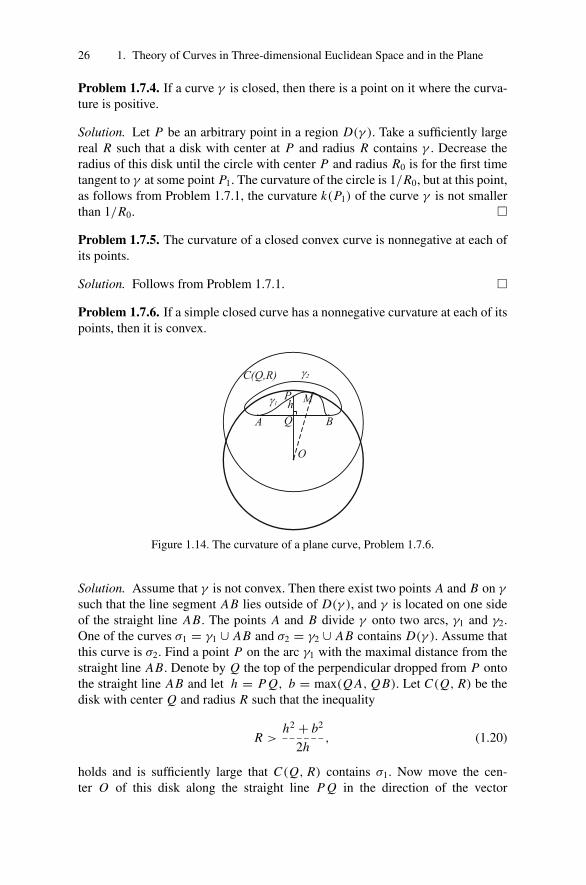
Problem 1.7.6. If a simple closed curve has a nonnegative curvature at each of itspoints, then it is convex.
Figure 1.14. The curvature of a plane curve, Problem 1.7.6.
Solution. Assume that γ is not convex. Then there exist two points A and B on γ
such that the line segment AB lies outside of D(γ ), and γ is located on one sideof the straight line AB. The points A and B divide γ onto two arcs, γ1 and γ2.One of the curves σ1 = γ1 ∪ AB and σ2 = γ2 ∪ AB contains D(γ ). Assume thatthis curve is σ2. Find a point P on the arc γ1 with the maximal distance from thestraight line AB. Denote by Q the top of the perpendicular dropped from P ontothe straight line AB and let h = P Q, b = max(Q A, Q B). Let C(Q, R) be thedisk with center Q and radius R such that the inequality
R >h2 + b2
2h, (1.20)
holds and is sufficiently large that C(Q, R) contains σ1. Now move the cen-ter O of this disk along the straight line P Q in the direction of the vector
1.7 Problems: Curvature of Plane Curves 27
−→P Q until C(Q, R) touches the curve σ1 at some point M . We shall prove thatM ∈ γ1 \ {A ∪ B}. In fact, if M = A or M = B, then O Q = O P − P Q < R −h,and consequently, O Q2 + b2 < (R − h)2 + b2 < R2 in view of the inequality(1.20). But O Q2 + b2 = R2, which is a contradiction. Hence M ∈ γ \ {A ∪ B}.The curvature k1 of γ1 relative to σ1 at M , in view of Problem 1.7.1, is not smallerthan 1/R, but with respect to γ it is equal to −R1 < −1/k, contrary to the condi-tion. �
Problem 1.7.7. If γ is a simple closed curve, then∫γ
k(s) ds = 2π.
Solution. Inscribe in a curve γ a closed polygonal line σ with the vertices
A1, A2, . . . , An, An+1 (An+1 = A1)
such that the integral curvature of every arc γi = Ai Ai+1 of γ is not greater thanπ . On each arc γi take a point Bi where the tangent line is parallel to the straightline Ai Ai+1. Denote by αi the inner angle of the polygonal line σ at the vertex Ai .Then
∫γi
k(s) ds = π −αi , where γi is the arc of γ from Bi to Bi+1. Consequently,
∫γ
k(s) ds =n∑
i=1
∫γi
k(s) ds = nπ −n∑
i=1
αi .
On the other hand,∑n
i=1 αi = π(n − 2) = nπ − 2π . Hence∫γ
k(s) ds = nπ − nπ + 2π = 2π. �
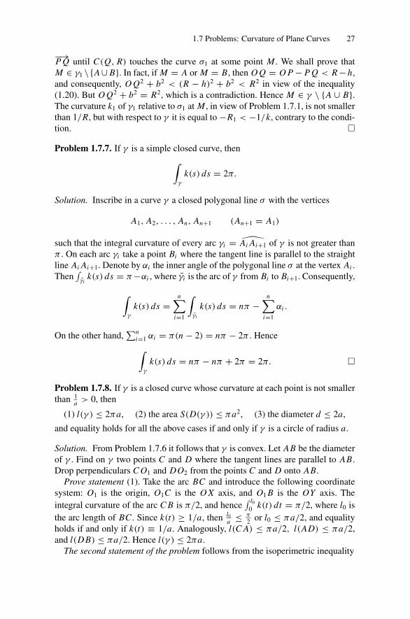
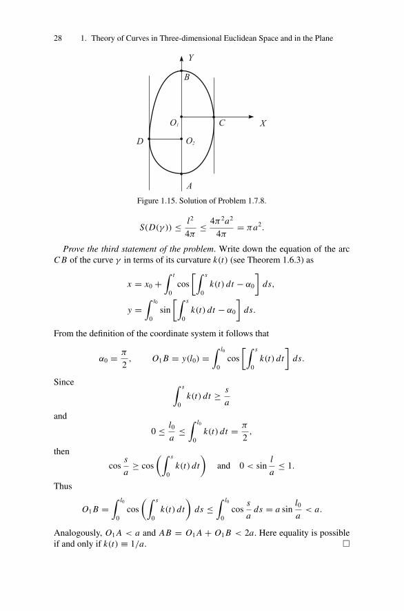
Problem 1.7.8. If γ is a closed curve whose curvature at each point is not smallerthan 1
a > 0, then
(1) l(γ ) ≤ 2πa, (2) the area S(D(γ )) ≤ πa2, (3) the diameter d ≤ 2a,
and equality holds for all the above cases if and only if γ is a circle of radius a.
Solution. From Problem 1.7.6 it follows that γ is convex. Let AB be the diameterof γ . Find on γ two points C and D where the tangent lines are parallel to AB.Drop perpendiculars C O1 and DO2 from the points C and D onto AB.
Prove statement (1). Take the arc BC and introduce the following coordinatesystem: O1 is the origin, O1C is the O X axis, and O1 B is the OY axis. Theintegral curvature of the arc C B is π/2, and hence
∫ l0
0 k(t) dt = π/2, where l0 isthe arc length of BC . Since k(t) ≥ 1/a, then l0
a ≤ π2 or l0 ≤ πa/2, and equality
holds if and only if k(t) ≡ 1/a. Analogously, l(C A) ≤ πa/2, l(AD) ≤ πa/2,and l(DB) ≤ πa/2. Hence l(γ ) ≤ 2πa.
The second statement of the problem follows from the isoperimetric inequality
28 1. Theory of Curves in Three-dimensional Euclidean Space and in the Plane
Figure 1.15. Solution of Problem 1.7.8.
S(D(γ )) ≤ l2
4π≤ 4π2a2
4π= πa2.
Prove the third statement of the problem. Write down the equation of the arcC B of the curve γ in terms of its curvature k(t) (see Theorem 1.6.3) as
x = x0 +∫ t
0cos
[∫ s
0k(t) dt − α0
]ds,
y =∫ t0
0sin
[∫ s
0k(t) dt − α0
]ds.
From the definition of the coordinate system it follows that
α0 = π
2, O1 B = y(l0) =
∫ l0
0cos
[∫ s
0k(t) dt
]ds.
Since ∫ s
0k(t) dt ≥ s
a
and
0 ≤ l0
a≤∫ l0
0k(t) dt = π
2,
then
coss
a≥ cos
(∫ s
0k(t) dt
)and 0 < sin
l
a≤ 1.
Thus
O1 B =∫ l0
0cos
(∫ s
0k(t) dt
)ds ≤
∫ l0
0cos
s
ads = a sin
l0
a< a.
Analogously, O1 A < a and AB = O1 A + O1 B < 2a. Here equality is possibleif and only if k(t) ≡ 1/a. �

1.7 Problems: Curvature of Plane Curves 29
Formulate and solve the dual problem to Problem 1.7.8 for convex curves.
Problem 1.7.9 (Problem about a bent bow). Let the arcs of convex curves γ1
and γ2 have the same length l. Assume that their curvatures k1(t) and k2(t) obeythe inequality k1(t) ≥ k2(t) ≥ 0 and let
∫ l0 k1(t) dt < π . Then γ1(0)γ1(l) ≤
γ2(0)γ2(l), and equality holds if and only if k1(t) ≡ k2(t).
Solution. Find a point γ1(s0) on the curve γ1 where the tangent line to γ1 is paral-lel to the chord γ1(0)γ1(l). Draw an orthogonal coordinate system in the followingway: γ1(s0) is the origin, the O X axis coincides with a tangent line to γ1, and theOY axis is orthogonal to the O X axis and directed to the chord γ1(0)γ1(l). Trans-late γ2 so that the point γ2(s0) coincides with γ1(s0) and the tangent line to γ2 at apoint γ2(s0) coincides with the O X axis. Denote by B the point of intersection ofthe OY axis with the chord γ1(0)γ1(l). The equations of the curves γ1 and γ2 inour coordinate system have the form
γ1 :{
x = x1(s) = ∫ ss0
cos[∫ s
s0k1(t) dt
]ds,
y = y1(s),
γ2 :{
x = x2(s) = ∫ s0 cos
[∫ ss0
k2(t) dt]
ds,y = y2(s).
Then x1(l) = Bγ1(l), and x2(l) is equal to the orthogonal projection of the chordγ1(s0)γ2(l) onto the O X axis. Prove that x1(l) ≤ x2(l). Since 0 <
∫ ss0
k(t) dt < π
for s0 < s < l, then
x1(l) =∫ l
s0
cos[∫ s
s0
k1(t) dt]
ds ≤∫ l
s0
cos[∫ s
s0
k2(t) dt]
ds = x2(l).
Analogously, x1(0) = |Bγ (0)| is not greater than the projection of the chordγ2(s0)x2(0) onto the O X axis. Thus γ1(0)γ1(l) is not greater than a sum of theorthogonal projections of the chords γ2(0)γ2(s0) and γ2(s0)γ2(l), which at thesame time is not greater than γ2(0)γ2(l). Equality holds if and only if k1(s) ≡k2(s). �
Problem 1.7.10. If γ is a closed curve whose curvature at each point is notsmaller than 1/a, then it can be rolled without sliding inside a disk of radius a.
Solution. First, consider the case k(t) > 1/a. Locate a circle C(a) of radius aso that the origin O belongs to C(a) and the O X axis (through the point O) istangent to C(a). Take an arbitrary point P on γ and locate γ so that P = O andthe tangent line to γ at P coincides with the O X axis. Let P1 be a point on γ
such that the arcs γ1 and γ2 into which γ is divided by the point P have integralcurvature π .
Introduce the arc length parameter s (counted from P) on γ1 and C(a). Thenα(s) = ∫ s
0 k(t) dt is not greater than π . We show that γ1 ∩ C(a) = ∅. If not, letP2 be the first point (starting from P) of intersection of γ1 with C(a). Write theequations of the curves γ and C(a):

30 1. Theory of Curves in Three-dimensional Euclidean Space and in the Plane
Figure 1.16. Solution of Problem 1.7.10.
γ1 :{
x = ∫ s0 cos α(s) ds,
y = y1(s),C(a) :
{x = ∫ s
0 cos( sa ) ds,
y = y2(s).
Then there exist numbers s2 and s1 such that∫ s2
0cos α(s) ds =
∫ s1
0cos
s
ads, P2 = γ (s2) = C(a)(s1).
Since α(s) = ∫ s0 k(t) dt > s
a , then cos α(s) < cos sa . Hence s2 > s1. But on
the other hand, the convex arc P P2 of γ1 lies entirely inside the arc P P2 of thecircle C(a) and the chord P P2. Thus s2 ≤ s1, which is a contradiction. Henceγ1 ∩ C(a) = ∅.
Analogously, one can prove that γ2 ∩ C(a) = ∅. Now if k(t) ≥ 1/a, then fromthe above, it follows that γ ∩ C(a + ε) = ∅ for every ε > 0. From this we get thatγ lies entirely inside of C(a). The problem is solved in view of the arbitrarinessof the point P . �
Formulate and solve the dual problem to Problem 1.7.10 for convex curves.
Problem 1.7.11. Let a curve γ touch the circle C(a) with center O and radius aat the points A and B and lie entirely inside of C(a), and suppose � AO B < π .Then the curvature at some point on γ is smaller than 1/a.
Solution. Consider a curve γ , composed from the greater circular arc of C(a) andof a curve γ . Assume that the curvature at all points of γ is not smaller than 1/a.
Figure 1.17. Solution of Problem 1.7.11.
Let P0 be a point on γ nearest to the center O of a circle C(a). Then O P0, by

1.7 Problems: Curvature of Plane Curves 31
conditions of the problem, is smaller than a. Denote by O1 a center of a circle ofa radius a, which touches γ at P0. Then this circle intersects γ , in contradictionto the statement of Problem 1.7.10. �
Problem 1.7.12. Let a curve γ touch a circle C(a) of radius a at the points A andB, located outside of C(a), and suppose � AO B < π . Prove that there is a pointon γ at which the curvature of γ is greater than 1/a.
Prove this problem on your own.
Figure 1.18. Solution of Problem 1.7.12.
In order to formulate the next problems, we give some definitions.
Let γ be any smooth closed convex curve. Denote by C(P, γ ) the circle satis-fying the following conditions:
(1) C(P, γ ) touches γ at the point P ,
(2) C(P, γ ) ⊂ D(γ ),
(3) C(P, γ ) has the maximal radius for which conditions (1) and (2) hold.
Denote by C+(γ ) a circle of maximal radius contained in D(γ ). Let C−(γ )
be a circle of minimal radius satisfying the conditions (1)–(3) (for some P ∈ γ ).Denote by R(P, γ ) the radius of C(P, γ ), and then write the radii of the circlesC+(γ ) and C−(γ ), respectively, as
R+(γ ) = supP∈γ
R(P, γ ), R−(γ ) = infP∈γ
R(P, γ ).
Problem 1.7.13. If C(P, γ ) ∩ γ = P , then the curvatures of γ and C(P, γ ) atthe point P are equal.
Solution. In view of Problem 1.7.1, the curvature kγ (P) of the curve γ at P isnot greater than 1/R(P, γ ). Assume that kγ (P) < 1/R(P, γ ). Take a monotonicsequence of numbers Rn satisfying the conditions
kγ (P) <1
Rn<
1
R(P, γ ), lim
n→∞ Rn = R(P, γ ).

32 1. Theory of Curves in Three-dimensional Euclidean Space and in the Plane
Figure 1.19. Solution of Problem 1.7.13.
Denote by C(P, γ, Rn) the circle of radius Rn that touches γ at P , in view of thedefinition of C(P, γ ). Then C(P, γ, Rn) intersects γ at least at one more pointPn �= P . Without loss of generality, assume that limn→∞ Pn = P exists. In viewof Problem 1.7.1, the point P cannot coincide with P . Consequently, P �= P andP ∈ γ ∩ C(P, γ ), which contradicts the condition of the problem. �
Problem 1.7.14. On an arbitrary closed semicircle of a circle C+(γ ) there is apoint that belongs to γ .
Solution. If not, let C be the closed semicircle of the circle C+(γ ) for whichC ∩ γ = ∅ holds. Denote by O the center of C+(γ ), and by R+ its radius. Drawthe diameter a through the ends of C . Denote by A1 and A2 the intersection pointsof the straight line containing the diameter a with γ . The points A1 and A2 divideγ into two arcs γ1 and γ2. Denote by γ1 one of these arcs satisfying the propertyγ1 ∩ C+(γ ) = ∅. Let d0 = minγ (s)∈γ1(Oγ (s) − R+) > 0. Drop the perpendicular
Figure 1.20. Solution of Problem 1.7.14.
to the line a from the center O inside of the semicircle C and then mark off theline segment O O1 = d0/2 = δ on it. For γ (s) ∈ γ1.
O1γ (s) − R+ > Oγ (s) − d0
2− R+ ≥ δ > 0.
For γ (s) ∈ γ2.
O1γ (s) − R+ =√
(Oγ (s))2 + δ2 − 2Oγ (s) · δ cos α − R+,
where α(s) is the angle in �O O1γ (s) at the vertex O . From the definition of O1
it follows that α(s) ≥ π/2. Hence

1.7 Problems: Curvature of Plane Curves 33
O1γ (s) − R+ ≥√
(Oγ (s))2 + δ2 − R+ ≥√
(R+)2 +δ2 − R+
= δ2√(R+)2 + δ2 + R+
= δ1 > 0.
But then the circle with center at O1 and radius R = R++σ > R+ lies entirely in-side of D(γ ), in contradiction to the definition of C+(γ ). Here σ = 1
2 min(δ, δ1).The reader should consider the case in which C+(γ ) ∩ γ consists of exactly twopoints. �
Problem 1.7.15. If γ is a closed convex curve of class C2, then the set C0 =C−(γ ) ∩ γ is connected.
Solution. C0 is a closed set. Consequently, the set γ \ C0 is the union of openarcs. If C0 is not connected, the number of these arcs γ1, γ2, . . . , γk is not smallerthan 2.
Two cases are possible:
(1) The integral curvature of one of these arcs is smaller than π .(2) C0 consists of two diametrically opposite points P1 and P2 of the circle
C−(γ ).
In the first case there is a point P1 on the arc γ1 at which the curvature kγ (P1)
is greater than 1/R−(γ ), but then R(P1, γ ) < R−(γ ), in contradiction to thedefinition of C−(γ ).
In the second case, for any point P ∈ γ, P �∈ C0, the value R(P, γ ) is notgreater than R−(γ ), because C(P, γ ) belongs, together with its curve γ , to thestrip of width 2R−(γ ) formed by the tangent lines to γ at the points P1 and P2.Hence, in this case the equality R(P, γ ) = R−(γ ) holds for all P . But thenγ = C(γ ), in contradiction to the assumption of nonconnectedness. �
Formulate and solve the dual problems to Problems 1.7.14 and 1.7.15.
Problem 1.7.16 (The four-vertex theorem).1 Prove that for any closed convexcurve of class C2 the curvature function k(s) has at least two local minima andtwo local maxima.
Note that a closed convex curve is sometimes called an oval. The converse ofthe four-vertex theorem is also true (H. Gluck, 1971): a function on a circle canbe realized as the curvature of a closed plane curve exactly if it admits at leasttwo maxima separated by two minima.
Solution. If C+(γ ) �= γ , then C1 = C+(γ ) ∩ γ divides γ \ C1 into open arcsγ1, γ2, . . . , γk , k ≥ 2. Moreover, either the integral curvature of at least two arcs,
1 There are various recent generalizations of four vertex theorem. See, for example, Sedykh, V.D.,The four-vertex theorem of a plane curve and its generalizations. (Russian. English summary).Soros. Obraz. Zh., Vol. 6, No. 9, 122–127, 2000; Tabachnikov, S. A four vertex theorem for poly-gons. Am. Math. Mon., vol. 107, No. 9, 830–833, 2000.
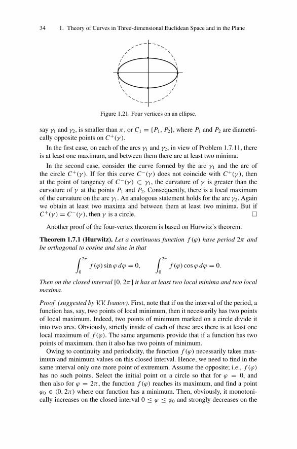
34 1. Theory of Curves in Three-dimensional Euclidean Space and in the Plane
Figure 1.21. Four vertices on an ellipse.
say γ1 and γ2, is smaller than π , or C1 = {P1, P2}, where P1 and P2 are diametri-cally opposite points on C+(γ ).
In the first case, on each of the arcs γ1 and γ2, in view of Problem 1.7.11, thereis at least one maximum, and between them there are at least two minima.
In the second case, consider the curve formed by the arc γ1 and the arc ofthe circle C+(γ ). If for this curve C−(γ ) does not coincide with C+(γ ), thenat the point of tangency of C−(γ ) ⊂ γ1, the curvature of γ is greater than thecurvature of γ at the points P1 and P2. Consequently, there is a local maximumof the curvature on the arc γ1. An analogous statement holds for the arc γ2. Againwe obtain at least two maxima and between them at least two minima. But ifC+(γ ) = C−(γ ), then γ is a circle. �
Another proof of the four-vertex theorem is based on Hurwitz’s theorem.
Theorem 1.7.1 (Hurwitz). Let a continuous function f (ϕ) have period 2π andbe orthogonal to cosine and sine in that∫ 2π
0f (ϕ) sin ϕ dϕ = 0,
∫ 2π
0f (ϕ) cos ϕ dϕ = 0.
Then on the closed interval [0, 2π ] it has at least two local minima and two localmaxima.
Proof (suggested by V.V. Ivanov). First, note that if on the interval of the period, afunction has, say, two points of local minimum, then it necessarily has two pointsof local maximum. Indeed, two points of minimum marked on a circle divide itinto two arcs. Obviously, strictly inside of each of these arcs there is at least onelocal maximum of f (ϕ). The same arguments provide that if a function has twopoints of maximum, then it also has two points of minimum.
Owing to continuity and periodicity, the function f (ϕ) necessarily takes max-imum and minimum values on this closed interval. Hence, we need to find in thesame interval only one more point of extremum. Assume the opposite; i.e., f (ϕ)
has no such points. Select the initial point on a circle so that for ϕ = 0, andthen also for ϕ = 2π , the function f (ϕ) reaches its maximum, and find a pointϕ0 ∈ (0, 2π) where our function has a minimum. Then, obviously, it monotoni-cally increases on the closed interval 0 ≤ ϕ ≤ ϕ0 and strongly decreases on the

1.7 Problems: Curvature of Plane Curves 35
closed interval ϕ0 ≤ ϕ ≤ 2π . It is easy to see that under these circumstances theintegrals are negative:∫ ϕ0
0f (ϕ) sin
(ϕ − ϕ0
2
)dϕ < 0,
∫ 2π
ϕ0
f (ϕ) sin(ϕ − ϕ0
2
)dϕ < 0.
Indeed, the sine term figured in them is symmetric on both intervals of integrationrelative to their midpoints ϕ0/2 and π + ϕ0/2; furthermore, on the region, wherethe sine is positive the values of a function f (ϕ) are smaller than on the region,where the sine is negative.
It is not difficult to translate these “geometric” arguments into the exact lan-guage of formulas. For example, the first of above integrals can be written in theform ∫ ϕ0/2
0
[f(ϕ + ϕ0
2
)− f
(ϕ − ϕ0
2
)]sin ϕ dϕ,
and we see clearly that it is negative. The second of the above integrals is trans-formed analogously. Thus, the sum of above two integrals is also negative;∫ 2π
0f (ϕ) sin
(ϕ − ϕ0
2
)dϕ < 0,
but by the condition it must be zero. �
Here is a second solution of Problem 1.7.16.
Proof (2). Assume without loss of generality that the curvature of the oval ispositive at each point. If L denotes the length of an oval and s is selected as an arclength parameter, then in Cartesian coordinates (x, y) our curve can be describedby the equations
x = x(s), y = y(s), 0 ≤ s ≤ L .
From Theorem 1.6.3 it follows that
x ′(s) = cos ϕ(s), y′(s) = sin ϕ(s), 0 ≤ ϕ(s) < 2π,
and let ϕ(0) = 0. The curvature of the oval is k(s) = ϕ′(s) (see Theorem 1.6.3).Since the curvature is positive, the angle ϕ = ϕ(s) is an increasing function of thevariable s, and hence an inverse function s = s(ϕ) exists. Writing for simplicityk(ϕ) = k(s(ϕ)), we see that the curvature k is a continuous 2π -periodic functionof ϕ. Note also that a function s = s(ϕ) has a derivative at each point ϕ, which iscalculated by the formula
ds
dϕ= 1
ϕ′(s(ϕ))= 1
k(ϕ).
From this follows ds = dϕ
k(ϕ). Now we are ready to present the solution of Prob-
lem 1.7.16.
36 1. Theory of Curves in Three-dimensional Euclidean Space and in the Plane
The function 1/k(ϕ) is orthogonal (in the integral sense) to both the cosine andthe sine of ϕ. Indeed, an oval is a closed curve, and hence∫ L
0x ′(s) ds =
∫ L
0y′(s) ds = 0.
But on the other hand, these integrals are∫ L
0cos ϕ(s) ds =
∫ 2π
0cos ϕ
dϕ
k(ϕ)and
∫ L
0sin ϕ(s) ds =
∫ 2π
0sin ϕ
dϕ
k(ϕ).
For finishing the proof, note that the functions k(ϕ) and 1/k(ϕ) have a commonextremum, and refer to Hurwitz’s theorem, Theorem 1.7.1. �
We shall formulate one more problem, whose solution (suggested by V.V.Ivanov) is also based on Hurwitz’s theorem.
Imagine a convex polygon contained in a vertical plane. Call each of the sideson which it can lean and remain on a horizontal straight line without overturningunder the action of gravity a base of the polygon. A base of a polygon is stableif the polygon standing on it would not drop under small rotations in the verticalplane in one or another direction. Clearly, at least one such base exists. But thesituation is much more interesting.
Problem 1.7.17 (The bases of a convex polygon). Any convex polygon has atleast two stable bases.
Proof. Introduce Cartesian coordinates (x, y) in the plane of a convex polygonM , taking as origin the “center of mass” of our convex figure, which, obviously,is located strictly inside of M . Note first that∫∫
Mx dx dy = 0,
∫∫M
y dx dy = 0,
and second, we may describe the boundary of M in terms of corresponding polarcoordinates (ρ, ϕ) by an equation of the form ρ = ρ(ϕ), where the polar radius ρ
constitutes a positive continuous function of the angular variable ϕ running from0 to 2π . Recomputing the above double integrals in polar coordinates, we easilyobtain two new equalities,∫ 2π
0�3(ϕ) cos ϕ dϕ = 0,
∫ 2π
0�3(ϕ) sin ϕ dϕ = 0.
Hence, by Hurwitz’s theorem, the cube of the polar radius, and so the polar radiusitself, has two minima. From elementary geometrical considerations it is clear thatthese two values of the polar radius show us in what directions the rays from theorigin to the sides of a polygon must be drawn in order to intersect the interiors ofthese sides exactly in a right angle. Such sides of the polygon will be the requiredstable bases. �
1.7 Problems: Curvature of Plane Curves 37
As we see from the solution of the problem, it remains true for arbitrarybounded convex regions if together with “bases” we speak about stable “pointsof support.”
Problem 1.7.18. Prove that if there is a circle intersecting an oval at 2n points,then there exist 2n vertices on this oval.
Hint. Use Problems 1.7.16 and 1.7.17.
Problem 1.7.19. Let γ be a simple regular closed curve of class C2. Denote byD(γ ) the region bounded by γ . Prove that if the curvature k(P) of γ at each pointP ∈ γ satisfies the inequality |k(P)| ≤ 1/a, then there is a disk of radius a lyingentirely in D(γ ).
Problem 1.7.19 was formulated by A. Fet and solved by V. Ionin.
Hint. For solving the problem one needs to consider and study the properties ofthe “central” set of a curve γ . The central set M of the region D(γ ) (a curve γ )consists of the points defined in the following way: Let Q ∈ γ . Denote by C(Q)
the disk of a maximal radius that touches γ at the point Q and inside D(γ ). Theset of the centers of the disks C(Q), when Q runs along the whole curve γ , formsthe set M .
Problem 1.7.20. The integral curvature of an infinite convex curve γ is notgreater than π .
Solution. Let γ (s) be the arc length parameterization of a curve γ , counted fromone of its points. We show that for any s1 and s2, the inequality
∫ s2
s1k(s) ds ≤ π
holds.If not, let s1 and s2 be numbers such that
∫ s2
s1k(s) ds = ω1 > π . Draw the
straight lines a1 and a2 that touch γ at the points γ (s1) and γ (s2), respectively.Since a1 and a2 are nonparallel, they intersect at some point A. Thus the region Dbounded by the line segments γ (s2)A, γ (s1)A, and the arc γ (s1)γ (s2) of γ that isdefined by the inequalities s1 ≤ s ≤ s2 is a convex compact region containing thewhole curve γ , contradicts the condition of the problem. Consequently, for any s1
and s2, the inequality∫ s2
s1k(s) ds ≤ π holds. �
Problem 1.7.21. If the curvature function k(s) of a curve γ (s) (−∞ < s < ∞)
is a positive strictly increasing function, then γ has no points of self-intersection.Here s is an arc length parameter starting from some point of γ .
Solution. If not, let s1 and s2 be real numbers such that γ (s1) = γ (s2) and the arcσ = γ (s1)γ (s2) of γ (s) has no other points of self-intersection for s1 ≤ s ≤ s2.Then the curve σ bounds some convex region D. Let C(0, R) be a disk of amaximal radius inscribed in D, the point O be its center, and R its radius.
From Problem 1.7.12 it follows that the circle C(0, R) touches σ at least at twopoints γ (s3) and γ (s4), where s1 < s3 < s2 and s1 < s4 < s2, and � γ (s3)Oγ (s4)
is not greater than π . But then from Problems 1.7.1 and 1.7.10 it follows that at
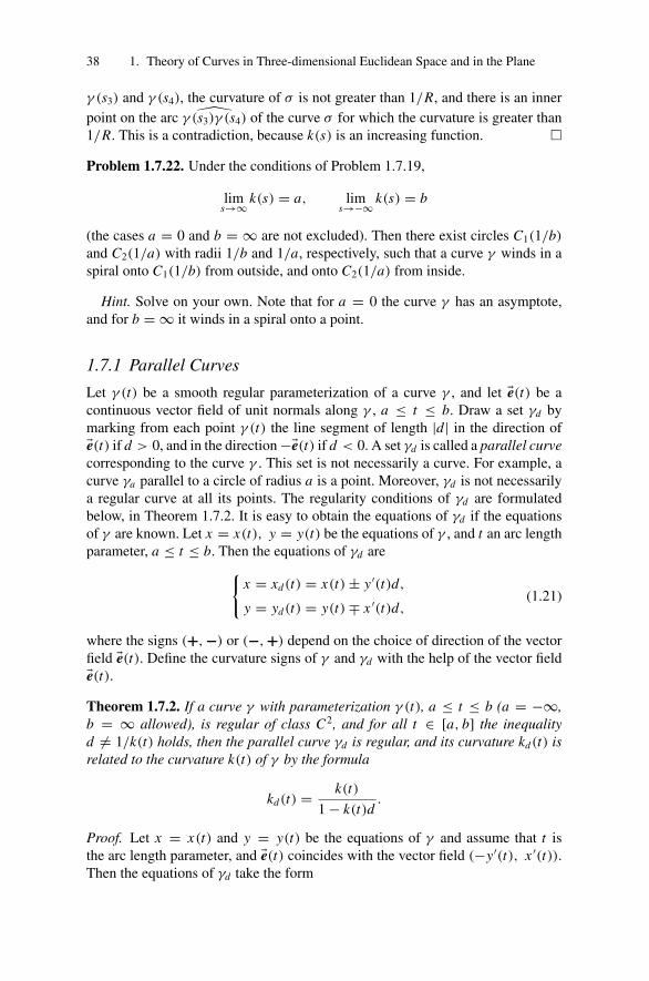
38 1. Theory of Curves in Three-dimensional Euclidean Space and in the Plane
γ (s3) and γ (s4), the curvature of σ is not greater than 1/R, and there is an innerpoint on the arc γ (s3)γ (s4) of the curve σ for which the curvature is greater than1/R. This is a contradiction, because k(s) is an increasing function. �
Problem 1.7.22. Under the conditions of Problem 1.7.19,
lims→∞ k(s) = a, lim
s→−∞ k(s) = b
(the cases a = 0 and b = ∞ are not excluded). Then there exist circles C1(1/b)
and C2(1/a) with radii 1/b and 1/a, respectively, such that a curve γ winds in aspiral onto C1(1/b) from outside, and onto C2(1/a) from inside.
Hint. Solve on your own. Note that for a = 0 the curve γ has an asymptote,and for b = ∞ it winds in a spiral onto a point.
1.7.1 Parallel Curves
Let γ (t) be a smooth regular parameterization of a curve γ , and let �e(t) be acontinuous vector field of unit normals along γ , a ≤ t ≤ b. Draw a set γd bymarking from each point γ (t) the line segment of length |d| in the direction of�e(t) if d > 0, and in the direction −�e(t) if d < 0. A set γd is called a parallel curvecorresponding to the curve γ . This set is not necessarily a curve. For example, acurve γa parallel to a circle of radius a is a point. Moreover, γd is not necessarilya regular curve at all its points. The regularity conditions of γd are formulatedbelow, in Theorem 1.7.2. It is easy to obtain the equations of γd if the equationsof γ are known. Let x = x(t), y = y(t) be the equations of γ , and t an arc lengthparameter, a ≤ t ≤ b. Then the equations of γd are{
x = xd(t) = x(t) ± y′(t)d,
y = yd(t) = y(t) ∓ x ′(t)d,(1.21)
where the signs (+, −) or (−, +) depend on the choice of direction of the vectorfield �e(t). Define the curvature signs of γ and γd with the help of the vector field�e(t).Theorem 1.7.2. If a curve γ with parameterization γ (t), a ≤ t ≤ b (a = −∞,b = ∞ allowed), is regular of class C2, and for all t ∈ [a, b] the inequalityd �= 1/k(t) holds, then the parallel curve γd is regular, and its curvature kd(t) isrelated to the curvature k(t) of γ by the formula
kd(t) = k(t)
1 − k(t)d.
Proof. Let x = x(t) and y = y(t) be the equations of γ and assume that t isthe arc length parameter, and �e(t) coincides with the vector field (−y′(t), x ′(t)).Then the equations of γd take the form
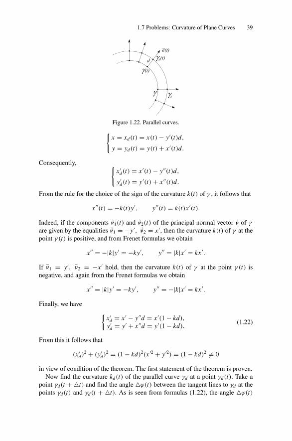
1.7 Problems: Curvature of Plane Curves 39
Figure 1.22. Parallel curves.{x = xd(t) = x(t) − y′(t)d,
y = yd(t) = y(t) + x ′(t)d.
Consequently, {x ′
d(t) = x ′(t) − y′′(t)d,
y′d(t) = y′(t) + x ′′(t)d.
From the rule for the choice of the sign of the curvature k(t) of γ , it follows that
x ′′(t) = −k(t)y′, y′′(t) = k(t)x ′(t).
Indeed, if the components �ν1(t) and �ν2(t) of the principal normal vector �ν of γ
are given by the equalities �ν1 = −y′, �ν2 = x ′, then the curvature k(t) of γ at thepoint γ (t) is positive, and from Frenet formulas we obtain
x ′′ = −|k|y′ = −ky′, y′′ = |k|x ′ = kx ′.
If �ν1 = y′, �ν2 = −x ′ hold, then the curvature k(t) of γ at the point γ (t) isnegative, and again from the Frenet formulas we obtain
x ′′ = |k|y′ = −ky′, y′′ = −|k|x ′ = kx ′.
Finally, we have {x ′
d = x ′ − y′′d = x ′(1 − kd),
y′d = y′ + x ′′d = y′(1 − kd).
(1.22)
From this it follows that
(x ′d)
2 + (y′d)
2 = (1 − kd)2(x ′2 + y′2) = (1 − kd)2 �= 0
in view of condition of the theorem. The first statement of the theorem is proven.Now find the curvature kd(t) of the parallel curve γd at a point γd(t). Take a
point γd(t + �t) and find the angle �ϕ(t) between the tangent lines to γd at thepoints γd(t) and γd(t + �t). As is seen from formulas (1.22), the angle �ϕ(t)

40 1. Theory of Curves in Three-dimensional Euclidean Space and in the Plane
is equal to the angle �θ(t) between the tangent lines to γ at the points γ (t) andγ (t + �t):
�ϕ(t) = �θ(t). (1.23)
The arc length �s of a curve γd between the points γd(t) and γd(t + �t) is givenby the formula
�s =∫ t+�t
t|1 − kd|dt. (1.24)
So from (1.23) and (1.24) it follows that
|kd(t)| = lim�t→0
�ϕ(t)
�s= lim
�t→0
�θ(t)
�t· lim
�t→0
�t
�s= |k(t)|
|1 − kd| . (1.25)
From the definition of the signs of the curvatures k(t) and kd(t) it is not difficult todeduce that for 1−kd > 0 the signs of k(t) and kd(t) coincide, but for 1−kd < 0these signs are opposite. Hence from (1.25) the second statement of the theoremfollows. �
Remark 1.7.1. If we define R(t) and Rd(t) by the formulas
R(t) = 1
k(t), Rd(t) = 1
kd(t),
then the last statement of Theorem 1.7.2 takes the form Rd = R − d .
Problem 1.7.23. Let γ (t) (−∞ < a ≤ t ≤ b < ∞) be a regular parameteriza-tion of a curve γ of the class C2. Prove that if
|d| < inft∈[a,b]
1
k(t),
then γd ∪ γ−d can be defined as a set of points whose distances from γ are equalto |d|.
Hint. If not, use Theorem 1.7.2 to obtain a contradiction.
Problem 1.7.24. Find a smooth regular curve, for which the parallel curves γd
have nonregular points for every d .
1.7.2 Evolutes and Evolvents
For regular curves of class C2 one may define a curve called an evolute of a givencurve γ .
Let γ (t) (a ≤ t ≤ b) have the property k(t) �= 0 for all t ∈ [a, b]. Then at eachpoint of γ the principal normal vector �ν(t) is defined. Mark off the line segment
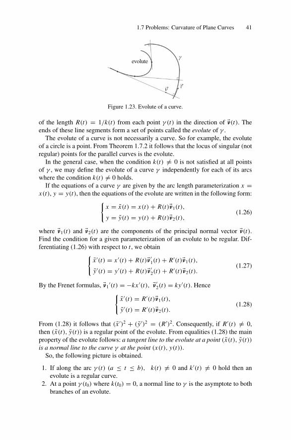
1.7 Problems: Curvature of Plane Curves 41
Figure 1.23. Evolute of a curve.
of the length R(t) = 1/k(t) from each point γ (t) in the direction of �ν(t). Theends of these line segments form a set of points called the evolute of γ .
The evolute of a curve is not necessarily a curve. So for example, the evoluteof a circle is a point. From Theorem 1.7.2 it follows that the locus of singular (notregular) points for the parallel curves is the evolute.
In the general case, when the condition k(t) �= 0 is not satisfied at all pointsof γ , we may define the evolute of a curve γ independently for each of its arcswhere the condition k(t) �= 0 holds.
If the equations of a curve γ are given by the arc length parameterization x =x(t), y = y(t), then the equations of the evolute are written in the following form:{
x = x(t) = x(t) + R(t)�ν1(t),
y = y(t) = y(t) + R(t)�ν2(t),(1.26)
where �ν1(t) and �ν2(t) are the components of the principal normal vector �ν(t).Find the condition for a given parameterization of an evolute to be regular. Dif-ferentiating (1.26) with respect to t , we obtain{
x ′(t) = x ′(t) + R(t)�ν ′1(t) + R′(t)�ν1(t),
y′(t) = y′(t) + R(t)�ν ′2(t) + R′(t)�ν2(t).
(1.27)
By the Frenet formulas, �ν1′(t) = −kx ′(t), �ν ′
2(t) = ky′(t). Hence{x ′(t) = R′(t)�ν1(t),
y′(t) = R′(t)�ν2(t).(1.28)
From (1.28) it follows that (x ′)2 + (y′)2 = (R′)2. Consequently, if R′(t) �= 0,then (x(t), y(t)) is a regular point of the evolute. From equalities (1.28) the mainproperty of the evolute follows: a tangent line to the evolute at a point (x(t), y(t))is a normal line to the curve γ at the point (x(t), y(t)).
So, the following picture is obtained.
1. If along the arc γ (t) (a ≤ t ≤ b), k(t) �= 0 and k ′(t) �= 0 hold then anevolute is a regular curve.
2. At a point γ (t0) where k(t0) = 0, a normal line to γ is the asymptote to bothbranches of an evolute.

42 1. Theory of Curves in Three-dimensional Euclidean Space and in the Plane
3. If at a point γ (t0) we have k(t) �= 0, but k ′(t) = 0 and k ′′(t) �= 0, then(x(t0), y(t0)) is a singular point of an evolute. At this point both regular arcsof the evolute meet: they have a common tangent line and are located in op-posite half-planes from it.
The case k ′(t0) = k ′′(t0) = 0 requires further investigation and is not treatedhere.
Now calculate the arc length s of the evolute between points with the parame-ters t1 and t2,
s =∫ t2
t1
√x ′2 + y′2dt =
∫ t2
t1
R′(t) dt = R(t2) − R(t1);
i.e., the arc length is equal to the difference in the radii of curvature of γ at thepoints γ (t2) and γ (t1).
Example 1.7.1. The evolute of the parabola x = t, y = at2 is the half-cubic(Neil’s) parabola xev = −4a2t3, yev = 3at2+ 1
2a . Its implicit equation is 27x2 =16a
(y − 1
2a
)3.
Definition 1.7.1. The evolvent of a curve γ is a curve γ such that its evolute is γ .
Figure 1.24. Evolvent of a curve.
Let x = x(t), y = y(t) be the arc length parameterization of γ . Then theequations of the evolvent γ may be written in the form{
x = x(t) = x(t) + a(t)x ′(t),y = y(t) = y(t) + a(t)y′(t). (1.29)
Find the function a(t) from the orthogonality of the vectors (x ′(t), y′(t)) and(x ′(t), y′(y)). Since
x ′(t) = x ′(t) + a(t)x ′′(t) + a′(t)x ′(t), y′(t) = y′(t) + a(t)y′′(t) + a′(t)y′(t),
we obtainx ′2(1 + a′) + y′2(1 + a′) = 0,
ora′(t) = −1,
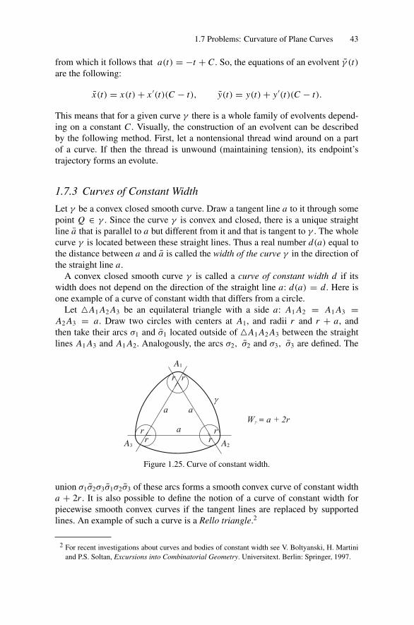
1.7 Problems: Curvature of Plane Curves 43
from which it follows that a(t) = −t + C . So, the equations of an evolvent γ (t)are the following:
x(t) = x(t) + x ′(t)(C − t), y(t) = y(t) + y′(t)(C − t).
This means that for a given curve γ there is a whole family of evolvents depend-ing on a constant C . Visually, the construction of an evolvent can be describedby the following method. First, let a nontensional thread wind around on a partof a curve. If then the thread is unwound (maintaining tension), its endpoint’strajectory forms an evolute.
1.7.3 Curves of Constant Width
Let γ be a convex closed smooth curve. Draw a tangent line a to it through somepoint Q ∈ γ . Since the curve γ is convex and closed, there is a unique straightline a that is parallel to a but different from it and that is tangent to γ . The wholecurve γ is located between these straight lines. Thus a real number d(a) equal tothe distance between a and a is called the width of the curve γ in the direction ofthe straight line a.
A convex closed smooth curve γ is called a curve of constant width d if itswidth does not depend on the direction of the straight line a: d(a) = d. Here isone example of a curve of constant width that differs from a circle.
Let �A1 A2 A3 be an equilateral triangle with a side a: A1 A2 = A1 A3 =A2 A3 = a. Draw two circles with centers at A1, and radii r and r + a, andthen take their arcs σ1 and σ1 located outside of �A1 A2 A3 between the straightlines A1 A3 and A1 A2. Analogously, the arcs σ2, σ2 and σ3, σ3 are defined. The
Figure 1.25. Curve of constant width.
union σ1σ2σ3σ1σ2σ3 of these arcs forms a smooth convex curve of constant widtha + 2r . It is also possible to define the notion of a curve of constant width forpiecewise smooth convex curves if the tangent lines are replaced by supportedlines. An example of such a curve is a Rello triangle.2
2 For recent investigations about curves and bodies of constant width see V. Boltyanski, H. Martiniand P.S. Soltan, Excursions into Combinatorial Geometry. Universitext. Berlin: Springer, 1997.

44 1. Theory of Curves in Three-dimensional Euclidean Space and in the Plane
It may be constructed by the following method: draw a circle of radius a withthe center at the vertex A1 of �A1 A2 A3, and take its smaller arc σ1 between A2
and A3. Analogously the arcs σ2 and σ3 are drawn. The union of arcs σ1σ2σ3
forms a convex closed curve of constant width a. The points A1, A2 and A3 arethe vertices of this curve, see Figure 1.26.
Figure 1.26. A Rello triangle.
Problem 1.7.25. Prove that the length of a curve of constant width a is πa.
Hint. Use the result of Problem 1.5.2.
Problem 1.7.26. Prove that if γ is a smooth curve of constant width b, and Q1
and Q2 are the points where the straight lines a1 and a2 touch γ , then the linesegment Q1 Q2 is orthogonal to a1 and a2, and consequently, Q1 Q2 = b.
Solution. Let P1 and P2 be the points of γ for which the length of the line segmentP1 P2 is equal to the diameter d of γ . Then the tangent lines to γ at the endpointsof this diameter are orthogonal to the line segment P1 P2. Consequently, d = b.Now let the points Q1 and Q2 have the properties given in the conditions of theproblem. Then
Q1 Q2 ≤ d = P1 P2 = b,
but also
Q1 Q2 ≥ b = d.
From these inequalities it follows that Q1 Q2 = b, and hence Q1 Q2 is orthogonalto a1 and a2. �
From the statements of the last problem it follows that at each point Q ∈ γ thereis a unique point Q∗ such that the tangent lines to γ at Q and Q∗ are parallel. Thepoints Q and Q∗ are called diametrically opposite points on the curve γ .
Problem 1.7.27. If γ is a curve of class C2 of the constant width a and the cur-vatures of γ at diametrically opposite points are equal, then γ is a circle of diam-eter a.
Hint. Use the result of Theorem 1.7.2.
1.8 Torsion of a Curve 45
Problem 1.7.28. Find analytic functions h such that the curve defined by theequations
x = h(θ) cos θ − dh
dθsin θ, y = h(θ) sin θ + dh
dθcos θ,
is a curve of constant width.
Hint. One of these functions is h(θ) = a + b cos(3θ) (0 < 8b < a), where a andb are real constants.
1.8 Torsion of a Curve
Let a curve γ be of class C2 and have nonzero curvature at a point P1. Then,by continuity, the curvature of γ is nonzero on some neighborhood of P1. Takean arbitrary point P2 in this neighborhood. By Theorem 1.6.2 there exist uniqueosculating planes α1 and α2 at the points P1 and P2. Denote by �θ the anglebetween them, and by �s the length of the arc P1 P2 of γ .
Definition 1.8.1. The value
κ = limP2→P1
�θ
�s= lim
�s→0
�θ
�s,
if it exists, is called the absolute torsion of the curve γ at the point P1.
If γ is a plane curve, then �θ ≡ 0 and the absolute torsion κ = 0. Below,we shall also prove the converse statement: if a curve γ has nonzero curvature ateach of its points and it has zero torsion, then γ is a plane curve.
The following theorem gives us sufficient conditions of the existence of torsionand a formula to derive it.
Theorem 1.8.1. If γ : �r = �r(t) is a regular curve of class C3, then at each of itspoints with nonzero curvature there is an absolute torsion κ , and
κ = |(�r ′ · �r ′′ · �r ′′′)|
|�r ′ × �r ′′| .
Proof. Let �r = �r(s) be the arc length parameterization of the curve. Assume thatthe curvature of γ at the point P1 = �r(s1) is nonzero. Then there is a real numberε > 0 such that for s ∈ (s1 − ε, s1 + ε) the curvature of γ at the points �r(s) is alsononzero. The angle between the osculating planes at the points P1 = �r(s1) andP2 = �r(s2) for s2 ∈ (s1 − ε, s1 + ε) is equal to the angle between the binormalvectors �β1(s) and �β2(s). Thus, |�β2(s2) − �β(s1)| = 2 sin �θ
2 . From this it followsthat
lim�s→0
�θ
�s= lim
�θ→0
�θ
2 sin �θ
2
· lims2→s1
|�β(s2) − �β(s1)||s2 − s1| = |�β ′
(s1)|.
46 1. Theory of Curves in Three-dimensional Euclidean Space and in the Plane
It remains to prove the existence of �β ′(s1), where �β(s) = �r ′×�r ′′
|�r ′×�r ′′| .The denominator of this expression for s = s1 is nonzero, since k(s1) =
|�r ′×�r ′′||�r ′|3 �= 0. Thus from the conditions of the theorem and the differentiation rule
for quotients the existence of �β ′(s1) follows. Transform the formula κ = |�β ′
(s1)|to a more convenient form for calculations. By definition, �β(s) = �τ (s) × �ν(s).
Hence �β ′ = �τ ′ × �ν + �τ × �ν ′. Since �τ ′ = �r ′′ss , but �ν = �r ′′
ss
|�r ′′ss | , then �τ ′ × �ν = 0 and
�β ′ = �τ × �ν ′. From this it follows that �β ′⊥�τ , and also that �β ′⊥�β. Hence �β ′ = λ�ν,where |λ| = |�β ′|. So, κ = |�β ′| = |〈�β ′
, �ν〉|, or κ = |〈�τ × �ν ′, �ν〉| = |(�τ · �ν · �ν ′
)|.Find �ν ′:
�ν = �r ′′ss
|�r ′′ss |
.
Hence �ν ′ = �r ′′′sss
|�r ′′ss | + A�r ′′, where A is some function of s. Substituting the expression
for �ν ′ into the formula for κ , we obtain
κ = (�τ · �ν · �ν ′)
|�r ′′| = |(�r ′ · �r ′′ · �r ′′′)|
|�r ′′| .
If �r = �r(t) is an arbitrary parameterization of class C3, then
�r ′s = �r ′
t
|�r ′t |
, �r ′′ss = �r ′′
t t
|�r ′t |2
+A�r ′t , �r ′′′
sss = �r ′′′t t t
|�r ′t |3
+B�r ′′t t+C�r ′
t , |�r ′′ss | = |�r ′
t × �r ′′t t |
|�r ′t |3
,
where A, B, and C are some functions of t . Thus
κ = |(�r ′t · �r ′′
t t · �r ′′′t t t )|
|�r ′t × �r ′′
t t |2. �
One may define the sign of the torsion for curves γ ⊂ R3: as we saw before,|�β ′| = |〈�β ′
, �ν〉|. Define the torsion by the formula κ = −〈�β ′, �ν〉. Geometrically,
this means that the torsion is positive if while moving along a curve the basis{�τ , �ν, �β} turns around �τ by the right-hand rule; i.e., clockwise as viewed fromthe initial point of the vector �τ .
Exercise 1.8.1. Find all curves of nonzero curvature and of zero torsion at all theirpoints.
Solution. Let κ = 0. Since |�β ′| = κ for the arc length parameterization, then�β ′ = 0. Consequently, �β(s) = �β0. Moreover, we already know that 〈�β, �τ 〉 = 0or 〈�r ′
, �β0〉 = 0, from which it follows that 〈�r(s) − �r(s0), �β0〉 = const. Hence thecurve γ is located in a plane orthogonal to the vector �β0; i.e., γ is a plane curve.
Note that the condition k �= 0 is not superfluous. Consider a curve γ , consistingof two arcs γ1 and γ2; γ1 is given by the equations y = x4, z = 0 (0 ≤ x <
∞), and γ2 is given by the equations y = 0, z = x4 (−∞ < x ≤ 0). Thecurvature of the obtained curve γ is defined at all points and is zero only at thepoint M0(0, 0, 0); the torsion is zero at every point where it is defined. Meanwhile,this γ is not a plane curve. �

1.9 The Frenet Formulas and the Natural Equation of a Curve 47
1.8.1 Formulas for Calculations
κ = (�r ′ · �r ′′ · �r ′′′)
|�r ′′|2 for the arc length parameterization �r = �r(s),
κ = (�r ′ · �r ′′ · �r ′′′)
|�r ′ × �r ′′|2 for an arbitrary parameterization �r = �r(t).
1.9 The Frenet Formulas and the Natural Equationof a Curve
For all points of a regular curve γ of class C3, where the curvature is nonzero,three mutually orthogonal unit vectors �τ , �ν, and �β (forming a basis) are uniquelydefined. Hence, any vector can be presented as their linear combination. In par-ticular, the vectors �τ ′, �ν ′, and �β ′
can be decomposed in terms of �τ , �ν, and �β. Ifa parameterization of a curve is natural, then the coefficients of the decomposi-tion have a geometrical sense, and they are expressed using the curvature and thetorsion. Indeed,
�τ (s) = �r ′(s), �τ ′ = �r ′′ = |�r ′′| · �r ′′
|r ′′| = k�ν,
and �β ′ = λ�ν, but from the definition torsion sign it follows that λ = −κ . Hence,
�β ′ = −κ�ν.
The three vectors {�τ , �ν, �β} form an orthogonal frame. Hence,
�ν = �β × �τ , �β = �τ × �ν, �τ = �ν × �β,
�ν ′ = �β ′ × �τ + �β × �τ ′ = −κ(�ν × �τ ) + k(�β × �ν) = κ �β − k�τ .
In such a way, we obtain formulas that are called the Frenet formulas:⎧⎨⎩�τ ′ = k�ν,
�ν ′ = −k�τ +κ �β,
�β ′ = −κ�ν,
(1.30)
or in matrix form, ⎛⎝ �τ ′
�ν ′
�β ′
⎞⎠ =⎛⎝ 0 k 0
−k 0 κ
0 −κ 0
⎞⎠⎛⎝ �τ�ν�β
⎞⎠ .
Using the Frenet formulas, it is easy to find the orthogonal projections of a curveonto the osculating plane (�τ , �ν), onto the normal plane (�ν, �β), and onto the rec-tifying plane (�τ , �β). Introduce a Cartesian coordinate system with the origin at

48 1. Theory of Curves in Three-dimensional Euclidean Space and in the Plane
a given point P = �r(s0) and with the coordinate axes directed along �τ , �ν, and�β; i.e., �τ = �i, �ν = �j , �β = �k. Apply Taylor’s formula to the vector function�r = �r(s):
�r(s) = �r(s0)+�r ′(s)(s −s0)+ 1
2�r ′′
(s0)(s −s0)2 + 1
6�r ′′′
(s0)(s −s0)3 +�o((s −s0)
3).
Since
�r(s0) = 0, �r ′(s0) = �τ (s0)�i, �r ′′
(s0) = k�ν = k �j , (1.31)
�r ′′′(s0) = k ′�ν(s0) + k�ν ′
(s0) = k ′�ν(s0) + k(−k�τ (s0) + κ �β(s0))
= −k2�i + k �j + kκ �k,
then ⎧⎪⎨⎪⎩x(s) = −s0 − 1
6 k2(s − s0)3 + o1((s − s0)
3),
y(s) = 12 k(s − s0)
2 + 16 k ′(s − s0)
3 + o2((s − s0)3),
z(s) = 16 kκ(s − s0)
3 + o3((s − s0)3).
From the last formulas we obtain the equations of the orthogonal projections
(1) onto the osculating plane: y = 12 kx2 + o(x3),
(2) onto the normal plane: z2 = Ay3 + o(y3), where A = 2κ2
9k ,(3) onto the rectifying plane: z = Bx3 + o(x3), where B = 1
6 kκ .
From the deduced equations it follows that the curvature of the projection of acurve onto the osculating plane is equal to the curvature of a given curve at thispoint, and the curvature of the projection onto the normal plane (at this point) iszero. This explains the notions of these planes.
For space curves there is a theorem analogous to the above theorem for theplane curves.
Theorem 1.9.1 (Fundamental Theorem of Curves). Let k(s) be an arbitrarycontinuous positive function, and κ(s) an arbitrary continuous function, 0 ≤ s ≤a. Then there is a unique (up to position in space) oriented curve for which k(s)is the curvature, and κ(s) is the torsion at the point corresponding to the end ofthe arc with arc length s.
Proof. If a curve γ with the given functions of curvature k(s) and torsion κ(s)exists, then the Frenet formulas (1.30) are satisfied for it. Hence to deduce theequations of γ it is natural to consider the Frenet formulas as a linear system ofODEs with the given functions k(s) and κ(s) as coefficients, in which we solve forthe vector functions �τ (s), �ν(s), and �β(s). One should also find the vector function�r(s) using �τ (s).
Let the functions �τ (s), �ν(s), and �β(s) be the solution of the system (1.30) withthe initial conditions �τ (0) = �τ 0, �ν(0) = �ν0, and �β(0) = �β0, and
1.9 The Frenet Formulas and the Natural Equation of a Curve 49
〈�τ 0, �τ 0〉 = 〈�ν0, �ν0〉 = 〈�β0,�β0〉 = 1,
〈�τ 0, �ν0〉 = 〈�τ 0, �β0〉 = 〈�ν0, �β0〉 = 0, (1.32)
(�τ 0 · �ν0 · �β0) = 1.
We wish to prove that the equalities (1.32) hold for any s. Introduce six newfunctions,
ξ1 = 〈�τ (s), �τ (s)〉, ξ2 = 〈�ν(s), �ν(s)〉, ξ3 = 〈�β(s), �β(s)〉,ξ4 = 〈�τ (s), �ν(s)〉, ξ5 = 〈�τ (s), �β(s)〉, ξ6 = 〈�ν(s), �β(s)〉,
and find the first derivatives of the functions ξi using the Frenet formulas:⎧⎪⎪⎪⎪⎪⎪⎪⎪⎪⎪⎨⎪⎪⎪⎪⎪⎪⎪⎪⎪⎪⎩
ξ ′1 = 〈�τ , �τ ′〉 = 2〈�τ ′
, �τ 〉 = 2kξ4,
ξ ′2 = 2〈�ν ′
, �ν〉 = 2〈−k�τ + κ �β, �ν〉 = −2kξ4 + 2κξ6,
ξ ′3 = 2〈�β ′
, �β〉 = 2〈−κ�ν, �β〉 = −2κξ6,
ξ ′4 = 〈�τ ′
, �ν〉 + 〈�τ , �ν ′〉 = kξ2 − kξ1 + κξ5,
ξ ′5 = 〈�τ ′
, �β〉 + 〈�τ , �β ′〉 = kξ6 − κξ4,
ξ ′6 = 〈�ν ′
, �β〉 + 〈�ν, �β ′〉 = −κξ2 + κξ3 − kξ5.
(1.33)
Consider the above system of equalities as a linear system of ODEs for unknownfunctions ξi , i = 1, . . . , 6, satisfying the initial conditions ξ1 = ξ2 = ξ3 =1, ξ4 = ξ5 = ξ6 = 0. From the uniqueness theorem for linear systems of ODEs itfollows that
ξ1(s) = ξ2(s) = ξ3(s) ≡ 1, ξ4(s) = ξ5(s) = ξ6(s) ≡ 0, (1.34)
and hence (�τ (s) · �ν(s) · �β(s)) = 1 by continuity.Now define the vector function �r(s) by the formula
�r(s) = �r0 +∫ s
0�τ (s) ds.
A curve γ given by this parameterization is required. Indeed, |�r ′(s)| = |�τ (s)| = 1.
Thus s is an arc length parameter counted from the point γ (0) = �r(0). Hence, inview of the Frenet formulas,
k(s) = |�r ′′(s)| = |�τ ′
(s)| = |k�ν(s)| = k(s).
Finally, κ = −〈�β ′, �ν〉 = −〈−κ�ν, �ν〉 = κ(s), again in view of the Frenet for-
mulas. Note that γ , generally speaking, is not a curve of class C3, but only ofclass C2. Nevertheless, it has torsion at each point. Thus, we obtain the followingresult:
Corollary 1.9.1. If the curvature of a curve γ is continuous, then γ belongs toclass C2, but from the continuity of the torsion it does not follow that γ belongsto class C3.
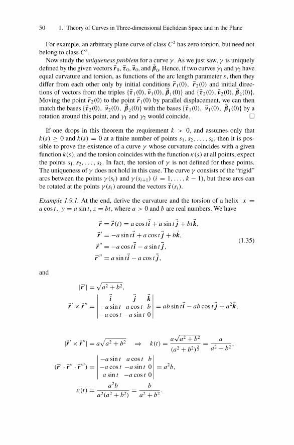
50 1. Theory of Curves in Three-dimensional Euclidean Space and in the Plane
For example, an arbitrary plane curve of class C2 has zero torsion, but need notbelong to class C3.
Now study the uniqueness problem for a curve γ . As we just saw, γ is uniquelydefined by the given vectors �r0, �τ 0, �ν0, and �β0. Hence, if two curves γ1 and γ2 haveequal curvature and torsion, as functions of the arc length parameter s, then theydiffer from each other only by initial conditions �r1(0), �r2(0) and initial direc-tions of vectors from the triples {�τ 1(0), �ν1(0), �β1(0)} and {�τ 2(0), �ν2(0), �β2(0)}.Moving the point �r2(0) to the point �r1(0) by parallel displacement, we can thenmatch the bases {�τ 2(0), �ν2(0), �β2(0)} with the bases {�τ 1(0), �ν1(0), �β1(0)} by arotation around this point, and γ1 and γ2 would coincide. �
If one drops in this theorem the requirement k > 0, and assumes only thatk(s) ≥ 0 and k(s) = 0 at a finite number of points s1, s2, . . . , sk , then it is pos-sible to prove the existence of a curve γ whose curvature coincides with a givenfunction k(s), and the torsion coincides with the function κ(s) at all points, expectthe points s1, s2, . . . , sk . In fact, the torsion of γ is not defined for these points.The uniqueness of γ does not hold in this case. The curve γ consists of the “rigid”arcs between the points γ (si ) and γ (si+1) (i = 1, . . . , k − 1), but these arcs canbe rotated at the points γ (si ) around the vectors �τ (si ).
Example 1.9.1. At the end, derive the curvature and the torsion of a helix x =a cos t, y = a sin t , z = bt , where a > 0 and b are real numbers. We have
�r = �r(t) = a cos t�i + a sin t �j + bt �k,
�r ′ = −a sin t�i + a cos t �j + b�k,
�r ′′ = −a cos t�i − a sin t �j ,�r ′′′ = a sin t�i − a cos t �j ,
(1.35)
and
|�r ′| =√
a2 + b2,
�r ′ × �r ′′ =∣∣∣∣∣∣
�i �j �k−a sin t a cos t b−a cos t −a sin t 0
∣∣∣∣∣∣ = ab sin t�i − ab cos t �j + a2�k,
|�r ′ × �r ′′| = a√
a2 + b2 ⇒ k(t) = a√
a2 + b2
(a2 + b2)32
= a
a2 + b2,
(�r ′ · �r ′′ · �r ′′′) =
∣∣∣∣∣∣−a sin t a cos t b−a cos t −a sin t 0a sin t −a cos t 0
∣∣∣∣∣∣ = a2b,
κ(t) = a2b
a2(a2 + b2)= b
a2 + b2.

1.10 Problems: Space Curves 51
We thus see that the curvature and the torsion of a helix are constants; i.e., donot depend on the parameter t . From Theorem 1.9.1 it follows that any curve ofconstant curvature k and constant torsion κ is a helix for which
a = k
k2 + κ2, b = κ
k2 + κ2.
1.10 Problems: Space Curves
In Section 1.10.1 we consider two problems about curves on a sphere. Then inSection 1.10.2 we shall formulate and solve some problems about space curves.
1.10.1 Spherical Curves
First we give some facts about spherical geometry. Let SR be a sphere of radius Rin R3. If P is some point on SR , denote by P∗ the point diametrically opposite P .If P and Q are arbitrary points on the sphere and Q �= P∗, then there is a uniquegreat circle C(P, Q) containing P and Q (this circle C(P, Q) is the intersectionof SR with the plane through the points P, Q and the center of the sphere SR). Thepoints P and Q divide C(P, Q) onto two arcs, the smaller one (by arc length) isdenoted by P Q. The length of this arc is denoted by ρ(P, Q) or simply by P Qand is called the distance between the points P and Q on the sphere SR .
It turns out that the length of any other curve with endpoints P and Q is greaterthan P Q. This statement will be proved in Chapter 3, but for now you shouldaccept it without proof. Thus a curve P Q is called a shortest path. Assume thatthe distance between the points P and P∗ is equal to π R; we call any arc of thegreat circle containing P and P∗ a shortest arc P P∗. It is clear that P and P∗may be joined by a shortest arc not uniquely, but possibly by an infinite numberof such arcs. Clearly, a closed curve γ on the sphere SR divides it into two regionsD1(γ ) and D2(γ ), each of them homeomorphic to a disk.
Definition 1.10.1. A region D on a sphere SR is convex if for any two points Pand Q located in D there is the shortest path P Q that belongs to D. A curve γ ona sphere SR is convex if one of the regions D1(γ ) or D2(γ ) is convex.
We now formulate a sequence of problems.
Problem 1.10.1. Prove that the length of any convex curve γ on the sphere SR isnot greater than 2π R, and that equality holds if and only if γ is a great circle, ora biangle (lune) formed by two shortest paths between some points P and P∗.
Solution. Let D be a convex region bounded by the curve γ .Consider the case that on γ there exist two diametrically opposite points P ,
P∗ ∈ γ . Draw one of the shortest paths (P P∗)1 that is located inside of D. Theexistence of the shortest path (P P∗)1 follows from the definition of a convex

52 1. Theory of Curves in Three-dimensional Euclidean Space and in the Plane
region. The shortest path (P P∗)1 divides D into two regions D1 and D2, and thepoints P and P∗ divide the curve γ into two arcs γ1 and γ2. Let γ1 belong tothe boundary of D1, and γ2 belong to the boundary of D2, and let l(γ1) ≥ l(γ2).Among all shortest paths between P and P∗ and containing D1, take (P P∗)2 thatforms a maximal angle with (P P∗)1. (It is not excluded that (P P∗)2 = (P P∗)1.)
To prove that γ1 = (P P∗)2, assume that γ1 �= (P P∗)2. Introduce on γ1 aparameterization γ1(t), where t is the arc length parameter, counting from thepoint P, 0 ≤ t ≤ l1 = l(γ1).
Define a function α(t) on [0, l1] equal to the angle between the shortest pathsPγ (t) and (P P∗)2 at the point P for t �= 0, and α(0) = limt→0 α(t). The last limitexists in view of the monotonicity of α(t). Analogously define the function β(t) asthe angle between the shortest paths P∗γ (t) and (P∗ P)2 at the point P∗ for t < land β(l) = limt→l β(t). Since 0 = β(0) ≤ α(0) and β(l) > α(l) = 0, then thereis a t0 such that α(t0) = β(t0) �= 0. But this means that the curve P γ (t0)∪γ (t0)P∗is the shortest path joining P with P∗ located inside of D and differing from(P P∗)2, which contradicts the definition of (P P∗)2. So, γ1 = (P P∗)2, and hencethe length l1 of the curve γ is π R. But then the inequality
π R ≤ l(γ2) ≤ l(γ1) = π R
holds, from which it follows that γ2 is the shortest path joining P with P∗ andthat the length of γ is 2π R.
In the second case draw a polygonal line p(γ ) inscribed in a curve γ withlength different from the length of γ by a sufficiently small value. Denote itsvertices by A1, A2, . . . , An . In view of the convexity of γ , the polygonal linep(γ ) is also convex, and the inner angle of every vertex in not greater than π :
� Ai , Ai+1 Ai+2 ≤ π, i = 1, . . . , n.
Extend the side A1 A2 to a great circle C(A1, A2). Since p(γ ) does not containthe diametrically opposite points, there is a minimal natural number i0 such thatAi0 /∈ C(A1, A2).
To prove that C(A1, A2) does not intersect the arc γ1 of a polygonal line p(γ )
taken from Ai0−1 to the point An+1 = A1, assume that C(A1, A2) ∩ γ1 �= ∅.Denote by B1 the first point of the intersection, counting from Ai1−1, and by B2
the last point of intersection. Then the circular arcs Ai1−1 B1 and B2 A1 are lo-cated outside of p(γ ). Neither of these arcs is the shortest path, and we obtaincontradiction with the convexity property of p(γ ). So, we have proved that thepolygonal line p(γ ) is located entirely inside a closed semisphere bounded by acircle C(A1, A2). From this, by standard methods, one can deduce that the lengthof p(γ ) is smaller than the length of C(A1, A2), which is equal to 2π R. Hencethe length of γ is also smaller than 2π R. �
Problem 1.10.2. Prove that if γ is a rectifiable closed curve on the sphere SR andthere is a great circle C on the sphere SR such that the intersection of any closedsemicircle C with γ is nonempty, then the length of γ is not smaller than 2π R.

1.10 Problems: Space Curves 53
Solution. Let T = C ∩ γ . Take an arbitrary point A1 ∈ T . The points A1 andA∗
1 divide C into two arcs, C1 and C2. Take a point A2 ∈ T on the arc C1 withmaximal distance from A1. In view of the conditions of the problem, such an A2
exists and differs from A1. If A2 = A∗1, then the problem is solved, because the
length of each of the arcs γ1 and γ2 of γ bounded by the points A1 and A∗1 is not
smaller than π R. If A2 �= A∗1, then again in view of the conditions of our problem,
there is a point A3 ∈ T on the arc A∗1 D ⊂ C2 of length π R − A2 A∗
1.So, we have obtained three points A1, A2, A3 ∈ T . Each of the arcs A1 A2,
A2 A3, and A3 A1 of C is a shortest one, and the sum of their lengths is 2π R. Butthe same points A1, A2, A3 divide γ into 3 arcs γ1 (from A1 to A2), γ2 (from A2
to A3), and γ3 (from A3 to A1), and their lengths are not smaller than the lengthsof certain arcs of C . Hence the length of γ is not smaller than 2π R. �
Problem 1.10.3. Prove that if a simple closed curve divides a sphere SR into tworegions with equal areas, then the length of γ is not smaller than 2π R.
Solution. Denote by D1 and D2 two regions into which γ divides SR . By thecondition of the problem, their areas are
S(D1) = S(D2). (1.36)
Let J be the map from a sphere SR onto itself transforming each point P into adiametrically opposite point P∗; i.e., J (P) = P∗. We shall prove that the curvesγ ∗ = J (γ ) and γ have nonempty intersection. Indeed, if γ ∗ ∩ γ = ∅, theneither D∗
1 = J (D1) ⊂ D2 or D∗2 = J (D2) ⊂ D1, which is impossible in view of
equality (1.36). Hence, γ ∩γ ∗ = T �= ∅. Let a point P ∈ T ; then the points P andP∗ belong to γ . Indeed, P ∈ γ and P ∈ γ ∗. Hence, P∗ = J (P) ∈ J (γ ∗) = γ .The points P and P∗ divide γ into two arcs γ1 and γ2, and each of them has lengthsmaller than π R. Thus the length of γ is not smaller than 2π R. �
Problem 1.10.4. Prove that if the length of a simple closed curve γ on the sphereSR is smaller than 2π R, then there is an open hemisphere S′
R of the sphere SR thatcontains γ .
Solution. A curve γ divides the sphere SR into two regions D1(γ ) and D2(γ ).One of these regions, in view of Problem 1.10.3, has area smaller than 2π R2.Let D1(γ ) be this region. Denote by K (P) the disk with center at a point P anda radius π2/R. Denote by S(P) the area of the intersection of the disks D1(γ )
and K (P0) and let S0 = infP∈SR S(P). Let K (P0) be the disk with the propertyS(P0) = S0. Let C(P) be a great circle, the boundary of the disk K (P), and letM = γ ∩C(P0). If M = ∅, then γ sits inside the open disk K (P∗
0 ). If M �= ∅, thenM ∈ C ′(P0), where C ′(P0) is some open semicircle C(P0); see Problem 1.10.2.
Denote by Q1 and Q2 the endpoints of C ′(P0), and let a = min ρ(γ, C(P0) \C ′(P0)). Now take a point P1 satisfying the following conditions:
(1) P1 is located in the region bounded by the arcs Q1 P0 ∪ P0 Q2 and C(P0) \C ′(P0).

54 1. Theory of Curves in Three-dimensional Euclidean Space and in the Plane
(2) The disk K (P1) contains the points Q1 and Q2,(3) π
2 R − a4 < ρ(P1, C(P0) \ C ′(P0)) < π
4 R + a4 .
Then the part of the disk K (P1) that is equal to K (P1) \ K (P) does not includethe points of D1(γ ), and the part of the disk K (P1) that is equal to K (P0)\ K (P1)
does not contain the points of D1(γ ), in view of the definition of the integer S0
and of the disk K (P0), because in the opposite case the area of the intersection ofD1(γ ) with K (P1) would be smaller than S0.
Consequently, S0 = 0 and D1(γ )∩ K (P0) = γ ∩C(P0) = ∅. But then the diskK (P1) has no common points with γ . �
1.10.2 Space Curves
Let γ (t) be a regular space curve of class Ck (k ≥ 1); let t be its arc length param-eter, and let �e be some unit vector. Draw a straight line a through the point γ (0)
in the direction of �e, and define the function p(t) as the length of the projectionof the vector
−−−−−→γ (0)γ (t) onto the line a, by taking into account the sign; i.e., we
assume p(t) = ⟨−−−−−→γ (0)γ (t), �e⟩.
Problem 1.10.5. Prove thatdp
dt= 〈�τ , �e〉.
Solution. If �r = �r(t) is a vector function that defines a curve γ , then−−−−−→γ (0)γ (t) =
�r(t) − �r(0) and p(t) = 〈�r(t) − �r(0), �e〉. From these we obtain dpdt = 〈 d�r
dt , �e〉 =〈�τ , �e〉. �
Corollary 1.10.1. If γ is closed curve with the length l, then∫ l
0〈�τ , �e〉 dt = 0 for any �e, |�e| = 1.
Corollary 1.10.2. Let d be the distance between the endpoints of a curve γ oflength l. Then
d = |γ (0)γ (l)| =∫ l
0〈�τ , �e〉 dt, where �e =
−−−−−→γ (0)γ (l)
|γ (0)γ (l)| .
Theorem 1.10.1 (Fenchel’s problem). The integral curvature of an arbitraryclosed space curve γ is not smaller than 2π ; equality holds if and only if γ isa convex plane curve.
Proof. Let γ (t) be an arc length parameterization of a curve γ with t (0 ≤ t ≤l = l(γ )). Define a curve σ(t) on a sphere S1 by associating with each pointγ (t) the end of the vector �τ (t) = γ (t) whose origin coincides with the centerof the sphere S1. The curve γ (t) is called the indicatrix of a tangent line to γ .The integral curvature of γ , defined by
∫ l0 k(t) dt , is equal to the length l1 of the
indicatrix of the tangent line σ(t). Indeed,
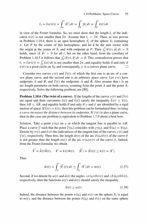
1.10 Problems: Space Curves 55
l1 = l(σ (t)) =∫ l
0|�τ ′| dt =
∫ l
0|k| dt =
∫ l
0k(t) dt
in view of the Frenet formulas. So, we must show that the length l1 of the indi-catrix σ(t) is not smaller than 2π . Assume that l1 < 2π . Then, as was provenin Problem 1.10.4, there is an open hemisphere S′
1 of the sphere S1 containingσ . Let P be the center of this hemisphere, and let �e be the unit vector withthe origin at the center of S1 and with endpoint at P . Then
∫ l0 〈�τ (t), �e〉 dt > 0
holds, since 〈�τ , �e〉 > 0 for all t , but on the other hand, from the corollary ofProblem 1.10.5 it follows that
∫ l0 〈�τ (t), �e〉 dt = 0. This contradiction proves that
l1 = l(σ (t)) = ∫ l0 k(t) dt is not smaller than 2π , and equality holds if and only if
σ(t) is a great circle on SR and consequently, γ is a convex plane curve. �
Consider two curves γ (t) and γ (t), of which the first one is an arc of a con-vex plane curve, and the second one is an arbitrary space curve. Let γ (t) haveendpoints A and B, and γ (t) the endpoints A and B. Also assume that t is anarc length parameter on both curves, counting from the point A and the point A,respectively. Solve the following problem; see [Bl].
Problem 1.10.6 (The twist of a curve). If the lengths of the curves γ (t) and γ (t)are equal and their curvatures k(t) and k(t) satisfy the inequality k(t) ≤ k(t),then AB ≤ A B, and equality holds if and only if γ and γ are identified by a rigidmotion of space. If k(t) = k(t), then this problem can be formulated thus: twistinga curve increases the distance between its endpoints. If γ (t) is also a plane curve,then in this case our problem is equivalent to Problem 1.7.9 about a bent bow.
Solution. Take a point γ (t0) on γ at which the tangent line is parallel to AB.Place a curve γ such that the point γ (t0) coincides with γ (t0), and �τ (t0) = �τ (t0).Denote by σ(t) and σ (t) the indicatrices of the tangent line of the curves γ (t) andγ (t), respectively. Then first, the length m(t) of the arc σ (t0)σ (t) of the curve σ
is not greater than the length m(t) of the arc σ(t0)σ (t) of the curve σ . Indeed,from the Frenet formulas we obtain
�τ ′ = k(t)�ν(t), �τ ′ = k(t)�ν(t), |�τ ′| = |k(t)| ≤ k(t) = |�τ ′|.Thus
m(t) =∫ t
t0
|�τ ′(t)| dt ≤
∫ t
t0
|�τ ′| dt = m(t). (1.37)
Second, if we denote by α(t) and α(t) the angles � σ(t0)Oσ(t) and � σ (t0)Oσ (t),respectively, then the functions α(t) and α(t) should satisfy the inequality
α(t) ≤ α(t). (1.38)
Indeed, the distance between the points σ(t0) and σ(t) on the sphere S1 is equalto m(t), and the distance between the points σ (t0) and σ (t) on the same sphere
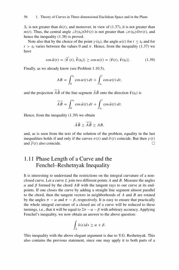
56 1. Theory of Curves in Three-dimensional Euclidean Space and in the Plane
S1 is not greater than m(t), and moreover, in view of (1.37), it is not greater thanm(t). Thus, the central angle � σ (t0)Oσ (t) is not greater than � σ(t0)Oσ(t), andhence the inequality (1.38) is proved.
Note also that by the choice of the point γ (t0), the angle α(t) for t ≤ t0 and fort > t0 varies between the values 0 and π . Hence, from the inequality (1.37) wehave
cos α(t) = 〈�τ ′(t), �τ (t0)〉 ≥ cos α(t) = 〈�τ (t), �τ (t0)〉. (1.39)
Finally, as we already know (see Problem 1.10.5),
AB =∫ t0
0cos α(t) dt +
∫ l
t0
cos α(t) dt,
and the projection A ¯B of the line segment A B onto the direction �τ (t0) is
A B =∫ t0
0cos α(t) dt +
∫ l
t0
cos α(t) dt.
Hence, from the inequality (1.39) we obtain
A B ≥ A B ≥ AB,
and, as is seen from the text of the solution of the problem, equality in the lastinequalities holds if and only if the curves σ(t) and σ (t) coincide. But then γ (t)and γ (t) also coincide. �
1.11 Phase Length of a Curve and theFenchel–Reshetnyak Inequality
It is interesting to understand the restrictions on the integral curvature of a non-closed curve. Let a curve L join two different points A and B. Measure the anglesα and β formed by the chord AB with the tangent rays to our curve at its end-points. If one closes the curve by adding a straight line segment almost parallelto the chord, then the tangent vectors in neighborhoods of A and B are rotatedby the angles π − α and π − β, respectively. It is easy to ensure that practicallythe whole integral curvature of a closed arc of a curve will be reduced to theseturnings, i.e., that it will be equal to 2π −α−β with arbitrary accuracy. ApplyingFenchel’s inequality, we now obtain an answer to the above question:∫
Lk(s)ds ≥ α + β.
This inequality with the above elegant argument is due to Y.G. Reshetnyak. Thisalso contains the previous statement, since one may apply it to both parts of a
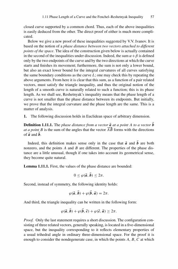
1.11 Phase Length of a Curve and the Fenchel–Reshetnyak Inequality 57
closed curve supported by a common chord. Thus, each of the above inequalitiesis easily deduced from the other. The direct proof of either is much more compli-cated.
Below we give a new proof of these inequalities suggested by V.V. Ivanov. It isbased on the notion of a phase distance between two vectors attached to differentpoints of the space. The idea of the construction given below is actually containedin the second of the inequalities under discussion. Indeed, the sum α+β is definedonly by the two endpoints of the curve and by the two directions at which the curvestarts and finishes its movement; furthermore, the sum is not only a lower bound,but also an exact lower bound for the integral curvatures of all curves satisfyingthe same boundary conditions as the curve L; one may check this by repeating theabove arguments. From here it is clear that this sum, as a function of a pair relatedvectors, must satisfy the triangle inequality, and thus the original notion of thelength of a smooth curve is naturally related to such a function; this is its phaselength. As we shall see, Reshetnyak’s inequality means that the phase length of acurve is not smaller than the phase distance between its endpoints. But initially,we prove that the integral curvature and the phase length are the same. This is amatter of analysis.
1. The following discussion holds in Euclidean space of arbitrary dimension.
Definition 1.11.1. The phase distance from a vector �a at a point A to a vector �bat a point B is the sum of the angles that the vector
−→AB forms with the directions
of �a and �b.
Indeed, this definition makes sense only in the case that �a and �b are bothnonzero, and the points A and B are different. The properties of the phase dis-tance are a little unusual, though if one takes into account its geometrical sense,they become quite natural.
Lemma 1.11.1. First, the values of the phase distance are bounded:
0 ≤ ϕ(�a, �b) ≤ 2π.
Second, instead of symmetry, the following identity holds:
ϕ(�a, �b) + ϕ(�b, �a) = 2π.
And third, the triangle inequality can be written in the following form:
ϕ(�a, �b) + ϕ(�b, �c) + ϕ(�c, �a) ≥ 2π.
Proof. Only the last statement requires a short discussion. The configuration con-sisting of three related vectors, generally speaking, is located in a five-dimensionalspace, but the inequality corresponding to it reflects elementary properties ofa usual trihedral angle in ordinary three-dimensional space. For the proof it isenough to consider the nondegenerate case, in which the points A, B, C at which

58 1. Theory of Curves in Three-dimensional Euclidean Space and in the Plane
vectors �a, �b, �c are attached do not lie on a straight line. Mark on the extensionsof the edges C A, AB, and BC of the triangle the points A′, B ′, and C ′. The leastvalue of the sum of the angles formed by the vector �a with the rays AA′ and ABis equal to the value of � A′ AB and is attained only in the case that �a lies in theplane of �ABC and varies within its specified exterior angle. In the same way,� B ′ BC and � C ′C A bound from below the sums of the other angles with verticesat B and C . From here it follows that the sum of the three phase distances underdiscussion, which breaks up into the sum of six angles adjoining the vectors �a, �b,�c, is not smaller than the sum of the exterior angles of �ABC , which is equal todouble the sum of its interior angles. �
Using the second statement of the lemma, the triangle inequality for phase dis-tances can be written down by the usual method:
ϕ(�a, �c) ≤ ϕ(�a, �b) + ϕ(�b, �c).Moreover as we have seen, this inequality turns into an exact equality only in thecase that the vectors �a, �b, �c lie in the corresponding exterior angles of �ABC .
2. Consider now a smooth curve L , determined by the arc length parameteriza-tion �r = �r(s) with 0 ≤ s ≤ l. Let s1 < s2 < · · · < sn , where s1 = 0, sn = land to the consecutive values of the parameter there correspond different pointson L . Draw at each of these points �r(si ) the tangent vector �τ i = �r ′
(si ). The chainthus obtained �τ 1, �τ 2, . . . , �τ n , is said to be a phase polygonal line inscribed in thecurve L , and its phase length is the sum
ϕ(�τ 1, �τ 2) + · · · + ϕ(�τ n−1, �τ n).
The phase length of the curve L should be defined as the infimum �(L) of thephase lengths of phase polygonal lines inscribed in it.
Lemma 1.11.2. If a chord joining the endpoints of a nonclosed curve L formsangles α and β with the tangent rays to the curve at its endpoints, then the phaselength of any phase polygonal line inscribed in L is not smaller than the sum ofthe angles α and β. In particular,
�(L) ≥ α + β.
If the curve L is closed, then the phase length at any phase polygonal line in-scribed in it is not smaller than 2π , so
�(L) ≥ 2π.
Proof. Indeed, in the first case, for every phase polygonal line �τ 1, �τ 2, . . . , �τ n
inscribed in L , the phase distance from �τ 1 up to �τ n is obviously equal to the sumof the specified angles, so by the triangle inequality,
α + β = ϕ(�τ 1, �τ n) ≤ ϕ(�τ 1, �τ 2) + · · · + ϕ(�τ n−1, �τ n).
1.11 Phase Length of a Curve and the Fenchel–Reshetnyak Inequality 59
In the case of a closed curve, when �τ 1 = �τ n , it is enough to apply the triangleinequality to the pair of vectors �τ 1, �τ n−1 and to note that ϕ(�τ 1, �τ n−1) = 2π −ϕ(�τ n−1, �τ n). �
By the way, if we take into account Section 1.9, it is easy to show that theinequalities in Lemma 1.11.2 become exact if and only if the curve either is a linesegment or lies in some plane where the vertices of any polygonal line inscribedin it serve as consecutive vertices of a convex polygon. This means that the curveis convex as a whole.
3. For studying the relations between the integral curvature of a curve and itsphase length, we need some asymptotic formulas describing the local geometryof a twice differentiable curve from the point of view of its curvature.
To simplify writing the expressions, use the symbol o(σ m) as the general des-ignation of any function possessing the property that after division by σ m it ap-proaches zero as σ → 0, uniformly with respect to other variables on which itmay depend.
For the arc length parameterization �r = �r(s) of a three-times differentiablecurve L , the tangent vector �τ (s) = �r ′
(s) has unit length and is orthogonal to�τ ′
(s), whose length, as was noted, is taken as a measure of the curvature k(s) ofthe curve L at the point with coordinate s.
Lemma 1.11.3. The following formulas hold:
〈�r(s + σ) − �r(s), �τ (s)〉 = σ − k2
6σ 3 + o(σ 3),
|�h(s)| = σ − k2
4σ 3 + o(σ 3),
〈�τ (s), �τ (s + σ)〉 = 1 − k2(s)
2σ 2 + o(σ 2),
where �h(s) = �r(s + σ) − �r(s) and σ > 0.
Proof. Applying Taylor’s formula and the Frenet formulas, we have
�r(s + σ) − �r(s) = �τ (s)σ + 1
2�τ ′
(s)σ 2+ 1
6�τ ′′
(s)σ 3 + o(σ 4)
= �τ (s)σ + 1
2k�ν(s)σ 2+ 1
6[k ′�ν(s) − k2�τ (s) + κ �β(s)]σ 3+ o(σ 4).
From this and from the properties of the Frenet frame the first formula of thelemma follows. Assume that �h(s) = �r(s +σ)−�r(s). Applying the above decom-position for the vector �h(s), we have
|�h(s)|2 = σ 2 + 1
4k2σ 4 − 1
3k2σ 4 + o(σ 4) = σ 2 − 1
12k2σ 4 + o(σ 4).
Taking the square root, we obtain the second equality of the lemma. The lastequality of the lemma can be proved analogously. �
60 1. Theory of Curves in Three-dimensional Euclidean Space and in the Plane
Remark 1.11.1. By elaborating the proof of the lemma, it is possible to obtain asimilar statement for a twice continuously differentiable curve.
4. Continuing considerations of a three-times differentiable curve, we return tothe question in which we are interested. First of all, write down the Taylor decom-position of the cosine,
〈�τ (s), �τ (s + σ)〉 = cos ω = 1 − ω2
2+ o(ω2),
where ω is the angle between the vectors �τ (s) and �τ (s + σ), and compare itwith the decomposition specified in Lemma 1.11.3. Indeed, we shall come to thewell-known equality
ω = k(s)σ + o(σ ),
characterizing the curvature as the velocity at which the angle ω grows as theparameter σ varies. As we shall now see, the phase distance, which generallydiffers from the usual angle between the vectors, is calculated for small parts of acurve by the same formula.
Lemma 1.11.4. The phase distance ϕ from a vector �τ (s) up to a vector �τ (s +σ)
for small σ > 0 is almost proportional to the arc σ
ϕ = k(s)σ + o(σ ).
Proof. By definition, ϕ is a sum of two angles ϕ1 and ϕ2 formed by the chord�h = �r(s + σ) − �r(σ ) with tangent vectors �τ (s) and �τ (s + σ). For calculating thecosine of the first of these angles, divide the decompositions in Lemma 1.11.3:
cos ϕ1 = 〈�h, �τ (s)〉|�h| = 1 − k2(s)
8σ 2 + o(σ 2).
We have already seen how from here it is possible to obtain the asymptotic for-mula
ϕ1 = k(s)
2σ + o(σ ).
By reversing the direction of the curve (which was determined by the choice ofparameterization, but played a minor role) the previous equality will transformto a similar expression for the cosine of the second angle ϕ2. One needs only toreplace k(s) by k(s+σ). However, it is possible to work without this replacement,as the difference between the two values as a function of σ is infinitesimally smalluniformly with respect to s. Thus,
ϕ2 = k(s)
2σ + o(σ ),
and it remains only to combine the two formulas into one. �
1.12 Exercises to Chapter 1 61
The following theorem, an integral version of Lemma 1.11.4, summarizes thediscussion so far. Comparing it with Lemma 1.11.2 allows us to look at theFenchel–Reshetnyak inequality from a new point of view.
Theorem 1.11.1. The phase length of a twice differentiable curve is equal to itsintegral curvature,
�(L) =∫
Lk(s) ds.
Proof. Select s1 < s2 < · · · < sn , where s1 = 0 and sn = l, in a closed interval0 ≤ s ≤ l. If all differences �si = si+1−si are small enough, then the neighboringpoints �r(si ) and �r(si+1) cannot coincide, and we have an opportunity to composethe sum
S =n−1∑i=1
ϕ(�τ (si ), �τ (si+1)).
The addition of new vertices to a phase polygonal line, in view of the triangleinequality, does not decrease its phase length. Therefore, the phase length of theinitial curve is equal to the limit of the sums under discussion, provided that thegreatest of the arcs �si tends to zero. According to Lemma 1.11.4, the sum S isexpressed as
S =n−1∑i=1
k(si )�si +n−1∑i=1
εi�si ,
where all εi uniformly tend to zero and simultaneously with �si . Thus, the secondterm of the last expression vanishes in the limit, and the first, as the integral sumfor the curvature, approaches its integral. �
1.12 Exercises to Chapter 1
Exercise 1.12.1. Let O be a point on a circle of radius a, and a ray intersectingthe circle at a varying point A rotates around O . Mark off two line segmentsAM1 = AM2 = 2a on this ray on two sides of A. Deduce the equation of a curvetraced by the points M1 and M2.Answer: a cardioid.
Exercise 1.12.2. A disk of radius a rolls along a straight line without sliding. De-duce the parametric equations of the curve traced by the point M on the boundarycircle.Answer: a cycloid.
Exercise 1.12.3. What curve is plotted by the parametric equations x = a log(t),y = a
2 (t + 1t )?
Exercise 1.12.4. Find the projections of the curve x = t, y = t2, z = t3 ontothe coordinate planes.
62 1. Theory of Curves in Three-dimensional Euclidean Space and in the Plane
Exercise 1.12.5. Prove that the projection onto the plane Y O Z of the intersectioncurve of an elliptical paraboloid x = y2 + z2 with a plane x − 2y + 4z = 0 is acircle of radius R = 3 centered at M(0, 1, −2).
Exercise 1.12.6. Find conditions for the existence of an asymptote to the spacecurve x = x(t), y = y(t), z = z(t) as t goes to infinity.
Exercise 1.12.7. Deduce the equations of the normal line and the tangent plane tothe helix x = 2 cos t, y = 2 sin t, z = 4t at the point t = 0.
Exercise 1.12.8. Deduce the equation of the tangent line to the curve x =cosh t, y = sinh t , z = ct .
Exercise 1.12.9. Deduce the equation of the main normal and binormal to thecurve
x = t, y = t2, z = t3, t = 1.
Exercise 1.12.10. Deduce the equation of the main normal and binormal to thecurve xy = z2, x2 + y2 = z2 + 1 at the point M(1, 1, 1).
Exercise 1.12.11. Deduce the equation of an osculating plane to the intersectioncurve of the sphere x2 + y2 + z2 = 9 and the hyperbolic cylinder x2 − y2 = 3 atthe point M(2, 1, 2).
Exercise 1.12.12. Deduce the equation of the tangent line to the curve defined bythe equations x2 + y2 + z2 = 1, x2 + y2 = x at the point M(0, 0, 1).
Exercise 1.12.13. Mark off the line segments of fixed length on the binormals toa simple helix. Find the equation of a curve that is traced by the endpoints of theseline segments.
Exercise 1.12.14. Prove the following generalizations of the well-known La-grange intermediate value theorem for the case of a smooth space curve.
1. Let A and B be the endpoints of a smooth space curve γ (t), and let � be asmooth family of tangent planes to γ . Then there is a value of the parametert0 such that the plane �(t0) is parallel to the line segment AB.
2. Let A and B be the endpoints of a smooth space curve γ (t) that belongs to aclosed convex surface. Then there is a value of the parameter t0 such that thetangent plane at the point γ (t0) is parallel to the line segment AB.
Exercise 1.12.15. Find the curvature and the torsion of the following curves:
(a) x = exp(t), y = exp(−t), z = t√
2,
(b) x = cos3 t, y = sin3 t, z = cos(2t).
Exercise 1.12.16. At what points of the curve x = a(t − sin t), y = a(1 − cos t),z = 4a cos t
2 does the radius of curvature take its local maximum?

1.12 Exercises to Chapter 1 63
Figure 1.27. Generalization of Lagrange’s intermediate value theorem.
Exercise 1.12.17. Prove that
(1) (�τ · �β · �β ′) = κ,
(2) (�β ′ · �β ′′ · �β ′′′) = κ2
(k
κ
)′,
(3) (�τ ′ · �τ ′′ · �τ ′′′) = k3
(κ
k
)′.
Exercise 1.12.18. Find the length of the curve x = a cosh t , y = a sinh t , z = atbetween the points 0 and t .
Exercise 1.12.19. Find the length of the astroid x = a cos3 t , y = a sin3 t.
Exercise 1.12.20. Find the length of the cycloid x = a(t −sin t), y = a(1−cos t)(0 ≤ t ≤ 2π).
Exercise 1.12.21. Find the curvature of the curve defined by the equations in im-plicit form
x + sinh x = y + sinh y, z + exp z = x + log(1 + x) + 1
at the point M(0, 0, 0).
Exercise 1.12.22. Find an evolute of the tractrix x = −a(log tan t
2 + cos t),
y = a sin t .
Exercise 1.12.23. Find the evolvent of the circle x2 + y2 = R2.
Exercise 1.12.24. Prove the constancy of the ratio of curvature to the torsion ofthe curve
x = a∫ t
t0
sin α(t) dt, y = a∫ t
t0
cos α(t) dt, z = bt.
Exercise 1.12.25.∗ Prove that a smooth curve γ (s) lies on a unit sphere if andonly if the following equality holds:
(k ′)2 = k2κ2(k2 − 1)
and k ≥ 1, where k = k(s), κ = κ(s) are the curvature and the torsion of thecurve γ (s).
2Extrinsic Geometry of Surfaces inThree-dimensional Euclidean Space
2.1 Definition and Methods of Generating Surfaces
Definition 2.1.1. A connected set � in R3 is said to be a two-dimensional surfaceif for an arbitrary point P ∈ � there exist an open ball UP in R3 with center atP and a continuous injective map ψ : UP → R3 such that ψ maps W = � ∩ UP
onto an open disk D1 of radius 1 on some plane α in the space R3.
In this definition, a “little” disk D1 can be replaced by an arbitrary open set3 ofa plane α, diffeomorphic to a disk. See Section 2.6 with further discussion of thenotion of a surface.
Introduce in the plane α Cartesian orthogonal coordinates u, v with the originat the center of the disk D1. Denote by ϕP the inverse of the restriction of themap ψ to D1. Then ϕP(D1) = W , and the map ϕP : D1 → R3 defines a vectorfunction �r = �r(u, v) = x(u, v)�i + y(u, v)�j + z(u, v)�k, where u2 + v2 < 1.We thereby obtain that a surface � in some neighborhood of one of its (arbitrary)points can be determined by three functions of two variables:
x = x(u, v), y = y(u, v), z = z(u, v).
These functions are called a parameterization of a surface. A parameterizationof a surface � is said to be k-fold continuously differentiable if the functionsx(u, v), y(u, v), and z(u, v) are actually k-fold continuously differentiable. The
3 A subset U ⊂ Rn is open if for every point x ∈ U there is a number ε > 0 such that y ∈ U
whenever ‖x − y‖ < ε.
66 2. Extrinsic Geometry of Surfaces in Three-dimensional Euclidean Space
set W = ϕP(D1) is called a coordinate neighborhood of the point P on thesurface �.
Definition 2.1.2. A surface � is k-fold continuously differentiable if in someneighborhood of each of its points there is a k-fold continuously differentiableparameterization x = x(u, v), y = y(u, v), z = z(u, v). In this case, we say thatthe surface � is of class Ck .
Definition 2.1.3. A surface � of class Ck (k ≥ 1) is regular if for each of itspoints P there is a parameterization ϕP : D1 → R3 of class Ck with maximalrank.4
The last condition can be written in the form �ru × �rv �= 0, where
�ru = xu(u, v)�i + yu(u, v)�j + zu(u, v)�k, �rv = xv(u, v)�i + yv(u, v)�j + zv(u, v)�k.
There are other presentations of a surface besides the parametric ones.
Explicitly given surface. Let f : D1 ⊂ R2 → R1 be a function of class Ck
(k ≥ 1). Then the set of points
{(x, y, f (x, y)) : (x, y) ∈ D1},the graph of a function f (x, y), forms a regular surface of class Ck . The equationof the surface in this case is usually written as x = x , y = y, z = f (x, y) orsimply as z = f (x, y), (x, y) ∈ D1.
Implicitly given surface. Let D be some open connected set of the space R3,let H : D → R1 be a differentiable map of class Ck , and let zero be a regularvalue of the map H . Then each connected component of the set � = H−1(0) is aregular surface of class Ck . The equation of the surface in this case can be writtenin the form H(x, y, z) = 0; it is called an implicit equation of the surface �. If aregular surface � is given by parametric equations
x = x(u, v), y = y(u, v), z = z(u, v),
then for each point P ∈ � there is a neighborhood in which � can be presented byan explicit equation. Indeed, since the rank of the map ϕP at the point P is 2, thenby the inverse function theorem the variables u and v can be expressed throughx, y; through x, z; or through y, z; and then the equation of � in a neighborhoodof P can be written in one of the following forms:
z = z(u(x, y), v(x, y)) = f1(x, y),
y = y(u(x, z), v(x, z)) = f2(x, z),
x = x(u(y, z), v(y, z)) = f3(y, z).
4 A Ck -coordinate patch for some k ≥ 1 is a one-to-one Ck -map x : D1 → R3 with maximal rank.
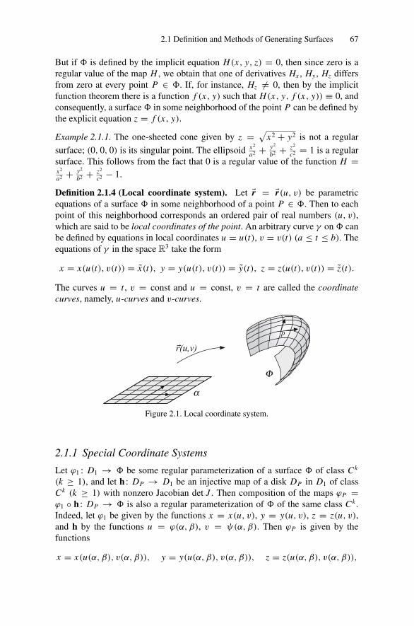
2.1 Definition and Methods of Generating Surfaces 67
But if � is defined by the implicit equation H(x, y, z) = 0, then since zero is aregular value of the map H , we obtain that one of derivatives Hx , Hy , Hz differsfrom zero at every point P ∈ �. If, for instance, Hz �= 0, then by the implicitfunction theorem there is a function f (x, y) such that H(x, y, f (x, y)) ≡ 0, andconsequently, a surface � in some neighborhood of the point P can be defined bythe explicit equation z = f (x, y).
Example 2.1.1. The one-sheeted cone given by z = √x2 + y2 is not a regular
surface; (0, 0, 0) is its singular point. The ellipsoid x2
a2 + y2
b2 + z2
c2 = 1 is a regularsurface. This follows from the fact that 0 is a regular value of the function H =x2
a2 + y2
b2 + z2
c2 − 1.
Definition 2.1.4 (Local coordinate system). Let �r = �r(u, v) be parametricequations of a surface � in some neighborhood of a point P ∈ �. Then to eachpoint of this neighborhood corresponds an ordered pair of real numbers (u, v),which are said to be local coordinates of the point. An arbitrary curve γ on � canbe defined by equations in local coordinates u = u(t), v = v(t) (a ≤ t ≤ b). Theequations of γ in the space R3 take the form
x = x(u(t), v(t)) = x(t), y = y(u(t), v(t)) = y(t), z = z(u(t), v(t)) = z(t).
The curves u = t , v = const and u = const, v = t are called the coordinatecurves, namely, u-curves and v-curves.
Figure 2.1. Local coordinate system.
2.1.1 Special Coordinate Systems
Let ϕ1 : D1 → � be some regular parameterization of a surface � of class Ck
(k ≥ 1), and let h : DP → D1 be an injective map of a disk DP in D1 of classCk (k ≥ 1) with nonzero Jacobian det J . Then composition of the maps ϕP =ϕ1 ◦ h : DP → � is also a regular parameterization of � of the same class Ck .Indeed, let ϕ1 be given by the functions x = x(u, v), y = y(u, v), z = z(u, v),and h by the functions u = ϕ(α, β), v = ψ(α, β). Then ϕP is given by thefunctions
x = x(u(α, β), v(α, β)), y = y(u(α, β), v(α, β)), z = z(u(α, β), v(α, β)),
68 2. Extrinsic Geometry of Surfaces in Three-dimensional Euclidean Space
and in view of well-known theorems from analysis, ϕP belongs to class Ck .To show the regularity of this parameterization, we have
�rα = �ruϕα + �rvψα, �rβ = �ruϕβ + �rvψβ.
Thus
|�rα × �rβ | = |�ru × �rv| · |ϕαψβ − ϕβψα| = |�ru × �rv| · det J �= 0,
which completes the proof.Sometimes, it appears necessary to introduce new coordinates on a surface so
that the curves from a given family become the coordinate curves. Often, we arriveat the following situation. In a given coordinate neighborhood W with coordinatesu, v, let two first-order differential equations are defined
A1(u, v) du + B1(u, v) dv = 0, A2(u, v) du + B2(u, v) dv = 0, (2.1)
and we wish to introduce a new coordinate system so that the integral curves ofequation (2.1) will become the coordinate curves. The following lemma gives usa sufficient condition for the existence of such a parameterization.
Lemma 2.1.1. If at the point P0(u0, v0) the determinant
det J =∣∣∣∣ A1(u0, v0) B1(u0, v0)
A2(u0, v0) B2(u0, v0)
∣∣∣∣is nonzero, then in some neighborhood of P0 one can introduce coordinates suchthat the integral curves of equation (2.1) will be the coordinate curves.
Proof. Rewrite (2.1) in the form of two systems of ordinary differential equations{dudt = −B1(u, v),
dvdt = A1(u, v),
(2.2){dudt = −B2(u, v),
dudt = A2(u, v).
(2.3)
Let γ0 be the integral curve of system (2.2) passing through P0, and let its equa-tions be given by the functions u = ϕ1(t), v = ψ1(t). Then the functions ϕ1(t),ψ1(t) satisfy the equations{
dϕ1
dt = −B1(ϕ1, ψ1),
dψ1
dt = A1(ϕ1, ψ1),and ϕ1(0) = u0, ψ1(0) = v0. (2.4)
Analogously, let σ0 be the integral curve of system (2.3) passing through the pointP0, and let u = ϕ2(τ ) and v = ψ2(τ ) be its equations. Then

2.1 Definition and Methods of Generating Surfaces 69{dϕ2
dτ= −B2(ϕ2, ψ2),
dψ2
dτ= A2(ϕ2, ψ2)
and ϕ2(0) = u0, ψ2(0) = v0. (2.5)
Denote by γτ (α) the integral curve of (2.2) passing through the point σ0(τ ), andby σt (β) the integral curve of (2.3) passing through γ0(t). Let P(t, τ ) be the pointof intersection of γτ (α) and σt (β). Since the coordinates of P(t, τ ) in W are u, v,then we obtain a map u = u(t, τ ), v = v(t, τ ). First, we prove that for sufficientlysmall t and τ the point P(t, τ ) is uniquely defined. This means that we must provethe existence and uniqueness of a solution of the system of equations{
F1(α, β, t, τ ) = f1(α, τ ) − f2(β, t) = 0,
F2(α, β, t, τ ) = h1(α, τ ) − h2(β, t) = 0,(2.6)
where u = f1(α, τ ), v = h1(α, τ ) are the equations of the curve γτ (α), andu = f2(β, t), v = h2(β, t) are the equations of the curve σt (β). From thedefinition of curves σ0, γ0, γτ (α), and σt (β) follow the equalities f1(0, 0) =u0 ± f2(0, 0), h1(0, 0) = v0 ± h2(0, 0). These equalities show us that the so-lution of the system (2.6) exists for t = τ = 0. We now calculate the determinant
det J1 =∣∣∣∣ F1,α F1,β
F2,α F2,β
∣∣∣∣ �= 0 at the point (0, 0):
F1,α = ∂ f1
∂α(0, 0) = ∂ f1
∂α(α, 0)|α=0 = ∂ϕ1
∂α|α=0 = −B1(u0, v0),
F1,β = −∂ f2
∂β(0, 0) = −∂ f2
∂β(β, 0)|β=0 = ∂ϕ2
∂β|β=0 = −B2(u0, v0),
F2,α = ∂h1
∂α(0, 0) = ∂h1
∂α(α, 0)|α=0 = ∂ψ1
∂α|α=0 = A1(u0, v0),
F2,β = −∂h2
∂β(0, 0) = −∂h2
∂β(β, 0)|β=0 = ∂ψ2
∂β|β=0 = A2(u0, v0).
(2.7)
From (2.7) we obtain
det J1 = − det J �= 0. (2.8)
From (2.8) and the implicit function theorem, we deduce the existence of a realδ > 0 such that for t2 + τ 2 < δ2 the functions α = α(t, τ ) and β = β(t, τ ) aredefined and differentiable. Note also that
α(t, 0) = t, β(0, τ ) = τ. (2.9)
The functions u = u(t, τ ) and v = v(t, τ ) are determined by the formulas
u = u(t, τ ) = f1(α(t, τ ), τ ) = f2(β(t, τ ), τ ),
v = v(t, τ ) = h1(α(t, τ ), τ ) = h2(β(t, τ ), τ ).(2.10)

70 2. Extrinsic Geometry of Surfaces in Three-dimensional Euclidean Space
The value of the determinant det J2 =∣∣∣∣∣ ∂u
∂t∂u∂τ
∂v∂t
∂v∂τ
∣∣∣∣∣ at the point t = τ = 0 is equal to
− det J , and hence det J2 �= 0. In fact, from (2.10), (2.9), and (2.7) it follows that
∂u
∂t= ∂ f1
∂α(0, 0) · ∂α
∂t
∣∣∣t=0
= −B1,∂u
∂τ= ∂ f2
∂β(0, 0) · ∂β
∂τ
∣∣∣τ=0
= −B2,
∂v
∂t= ∂h1
∂α(0, 0) · ∂α
∂t
∣∣∣t=0
= A1,∂v
∂τ= ∂h2
∂β(0, 0) · ∂β
∂τ
∣∣∣τ=0
= A2.
We apply again the inverse function theorem and obtain that the map u = u(t, τ ),v = v(t, τ ) induces new coordinates t and τ , for which t = const, τ = τ andt = t , τ = const are integral curves of equations (2.2) and (2.3). �
We prove one more lemma.
Lemma 2.1.2. Let �λ = λ1�ru + λ2�rv and �µ = µ1�ru + µ2�rv be two nonparallelvectors at the point P0(u0, v0). Then there is a coordinate system ξ, η such that Pis the point (0, 0) and �rξ = �λ, �rη = �µ.
Proof. Let the functions u = u(ξ, η) and v = v(ξ, η) be defined by the formulas
u = λ1ξ + µ1η + u0, v = λ2ξ + µ2η + v0.
Then the coordinates of the point P are (0, 0), and
�rξ = �ru∂u
∂ξ+ �rv
∂v
∂ξ= λ1�ru + λ2�rv = �λ,
�rη = �ru∂u
∂η+ �rv
∂v
∂η= µ1�ru + µ2�rv = �µ. �
2.2 The Tangent Plane
Let γ (t) : u = u(t), v = v(t) (a ≤ t ≤ b) be some curve through the pointP = γ (0) = (u(0), v(0)). A tangent vector γ = �τ to γ at P can be written inthe form γ = �r ′
t = �ruu′ + �rvv′. From this formula we see that the tangent vector
to any curve on the surface � through the point P belongs to the plane of vectors�ru(P) and �rv(P). This observation leads us to the following definition.
Definition 2.2.1. The plane through a point P of a regular surface � of class Ck
(k ≥ 1) that is parallel to the vectors �ru(P) and �rv(P) is called the tangent planeto the surface � at P . The normal to the surface � is an orthogonal vector to thetangent plane of the surface at the point P .
The normal to the surface � at the point P will be denoted by �n(P) and as-sumed to be a unit vector: |�n(P)| = 1. In particular, the normal can be identifiedwith the vector �ru�rv
|�ru�rv | .
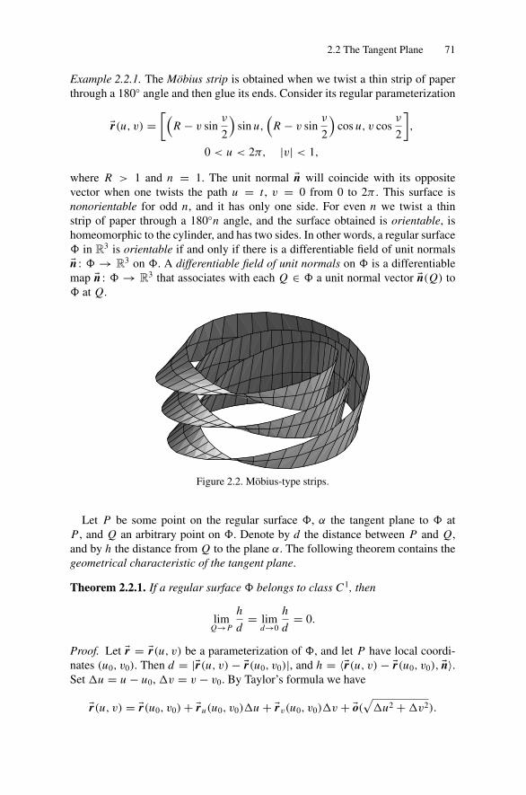
2.2 The Tangent Plane 71
Example 2.2.1. The Mobius strip is obtained when we twist a thin strip of paperthrough a 180◦ angle and then glue its ends. Consider its regular parameterization
�r(u, v) =[(
R − v sinν
2
)sin u,
(R − v sin
ν
2
)cos u, v cos
ν
2
],
0 < u < 2π, |v| < 1,
where R > 1 and n = 1. The unit normal �n will coincide with its oppositevector when one twists the path u = t , v = 0 from 0 to 2π . This surface isnonorientable for odd n, and it has only one side. For even n we twist a thinstrip of paper through a 180◦n angle, and the surface obtained is orientable, ishomeomorphic to the cylinder, and has two sides. In other words, a regular surface� in R3 is orientable if and only if there is a differentiable field of unit normals�n : � → R3 on �. A differentiable field of unit normals on � is a differentiablemap �n : � → R3 that associates with each Q ∈ � a unit normal vector �n(Q) to� at Q.
Figure 2.2. Mobius-type strips.
Let P be some point on the regular surface �, α the tangent plane to � atP , and Q an arbitrary point on �. Denote by d the distance between P and Q,and by h the distance from Q to the plane α. The following theorem contains thegeometrical characteristic of the tangent plane.
Theorem 2.2.1. If a regular surface � belongs to class C1, then
limQ→P
h
d= lim
d→0
h
d= 0.
Proof. Let �r = �r(u, v) be a parameterization of �, and let P have local coordi-nates (u0, v0). Then d = |�r(u, v) − �r(u0, v0)|, and h = 〈�r(u, v) − �r(u0, v0), �n〉.Set �u = u − u0, �v = v − v0. By Taylor’s formula we have
�r(u, v) = �r(u0, v0) + �ru(u0, v0)�u + �rv(u0, v0)�v + �o(√
�u2 + �v2).

72 2. Extrinsic Geometry of Surfaces in Three-dimensional Euclidean Space
Figure 2.3. Geometrical characteristic of a tangent plane.
Thus,
d = |�ru(u0, v0)�u + �rv(u0, v0)�v + �o(√
�u2 + �v2)|,h = 〈�ru(u0, v0)�u + �rv(u0, v0)�v + �o(
√�u2 + �v2), �n〉
= |〈�o(√
�u2 + �v2), �n〉| = �o1(√
�u2 + �v2).
From the last formulas it follows that
limd→0
h
d= lim
d→0
�o1(√
�u2 + �v2)
|�ru(u0, v0)�u + �rv(u0, v0)�v + �o(√
�u2 + �v2)| .
Divide the numerator and denominator of the above fraction by√
�u2 + �v2.We shall prove that the expression
|�ru(u0, v0)�u + �rv(u0, v0)�v + �o(√
�u2 + �v2)|√�u2 + �v2
is bounded from below by some positive number. For this, set ξ = �u√�u2+�v2 ,
η = �v√�u2+�v2 and note that ξ 2 + η2 = 1. We first estimate
|�ruξ + �rvη|2 = 〈�ru, �ru〉ξ 2 + 2〈�ru, �rv〉ξη + 〈�rv, �rv〉η2.
We shall introduce the notation
E = 〈�ru, �ru〉, F = 〈�ru, �rv〉, G = 〈�rv, �rv〉and calculate
EG − F2 = |�ru |2 · |�rv|2 − |�ru |2 · |�rv|2 cos2 ϕ = |�ru |2 · |�rv|2 sin2 ϕ = |�ru × �rv|2.Here ϕ represents the angle between the vectors �ru and �rv . Since the surface � isregular, |�ru × �rv| �= 0 and consequently, EG − F2 > 0. Hence, the fundamentalform Eξ 2 + 2Fξη + Gη2 is positive definite. But then
minξ 2+η2=1
|Eξ 2 + 2Fξη + Gη2| = a2 > 0.
From the last inequality it follows that
2.2 The Tangent Plane 73
|�ru�u + �rv�v + �o(√
�u2 + �v2)|√�u2 + �v2
≥ a
2
if√
�u2 + �v2 is sufficiently small. Thus, we have that the denominator of thefraction is bounded from below by a positive number, and the numerator tends tozero. Hence, limd→0
hd = 0, which completes the proof. �
Next, denote by T �P the tangent plane to � at P . The vectors �ru , �rv arelinearly independent and hence form a vector space basis of T �P called a localbasis of a surface � at a point P .
Definition 2.2.2. Let α be some plane in the space R3, and �e be a unit vectororthogonal to it. The pair (α, �e) is called an orientable plane.
This definition is motivated by the fact that an orientation on a plane α is de-termined by a given orientation on R3 and a vector �e. And conversely, from anorientation on α and on R3 we can reconstruct a vector �e. Each orientable planein the space generates in R3 a height function fα relative to a unit vector �e, definedby the formula
fα(P) = 〈−−→P0 P, �e〉,where P0 ∈ α is an arbitrary point. Obviously, fα does not depend on the choiceof P0.
Exercise 2.2.1. Prove that if Q is a critical point of the height function fα re-stricted to a regular surface �, then the tangent plane T �Q is parallel to the planeα.
Exercise 2.2.2. Prove that for almost every plane α that intersects a regular sur-face � of class Ck , the intersection α ∩ � is a regular curve of class Ck .
2.2.1 Formulas for Calculations
The surface is given by parametric equations.
�r = �r(u, v) = x(u, v)�i + y(u, v)�j + z(u, v)�k.
Then�ru = xu�i + yu �j + zu
�k, �rv = xv�i + yv
�j + zv�k.
Thus the equation of the tangent plane to a surface at the point (u0, v0) is writtenin the form
(yuzv − zu yv) · (X − x(u0, v0)) + (zu xv − xuzv) · (Y − y(u0, v0))
+ (xu yv − yu xv) · (Z − z(u0, v0)) = 0,
where X, Y, Z are coordinates of an arbitrary point in the plane, and all derivativesare calculated at the point (u0, v0).
74 2. Extrinsic Geometry of Surfaces in Three-dimensional Euclidean Space
Explicitly given surface. x = x , y = y, z = f (x, y).
�r x = �i + fx�k, �r y = �j + fy
�k, �r x × �r y = − fx�i − fy �j + �k.
Let the coordinates of the point of tangency be (x0, y0, z0) = f (x0, y0). Then theequation of the tangent plane takes the form
Z − z0 = fx (x0, y0)(X − x0) + fy(x0, y0)(Y − y0).
Implicitly given surface. H(x, y, z) = 0. Let (x0, y0, z0) be the point on asurface. The equation of the tangent plane to the surface at this point has the form
Hx (x0, y0, z0)(X − x0) + Hy(x0, y0, z0)(Y − y0) + Hz(x0, y0, z0)(Z − z0) = 0.
2.3 First Fundamental Form of a Surface
Let P be an arbitrary point on a regular surface �. In the tangent plane T �P wetake two vectors �λ and �µ. Let λ1, λ2 and µ1, µ2 be coordinates of these vectors �λand �µ in a local basis �ru(P) and �rv(P). Find a formula for calculation of a scalarproduct of �λ and �µ in terms of coordinates of these vectors in a local basis. Usingour above notation E = 〈�ru, �ru〉, F = 〈�ru, �rv〉, G = 〈�rv, �rv〉, we obtain
〈�λ, �µ〉 = Eλ1µ1 + F(λ1µ2 + λ2µ1) + Gλ2µ2.
In this way a scalar product generates on the surface � (in each tangent plane to�) a field of symmetric bilinear forms
I (�λ, �µ) = Eλ1µ1 + F(λ1µ2 + λ2µ1) + Gλ2µ2.
In particular, the first fundamental form of a surface is defined as
I (�λ) = I (�λ, �λ) = E(λ1)2 + 2Fλ1λ2 + G(λ2)2.
2.3.1 Length of a Curve on a Surface
Now let some smooth curve γ lie on a surface �, and let u = u(t), v = v(t)(a ≤ t ≤ b) be its equations in local coordinates. Find a formula for the lengthl(γ ) of γ . By the formula for the length of a curve, see Section 1.4, we have
l(γ ) =∫ b
a|�r ′| dt =
∫ b
a
√I (�r ′
) dt =∫ b
a
√E(u′)2 + 2Fu′v′ + G(v′)2 dt. (2.11)
The formula (2.11) can be written in the form
l(γ ) =∫ b
a
√E du2 + 2F du dv + G dv2, (2.12)
2.3 First Fundamental Form of a Surface 75
and the first fundamental form itself in the form
ds2 = E du2 + 2F du dv + G dv2.
In this case, ds is said to be an element of arc length. This type of notation for thefirst fundamental form is classical. The formula (2.11) shows us that knowledgeof the coefficients of the first fundamental form and the equations of a curve inlocal coordinates allow us to calculate the length of a curve.
Remark 2.3.1. If the equations of a surface are given, then in principle, we possesscomplete knowledge about the surface and its geometric properties. If the equa-tion of a surface is unknown, but only the first fundamental form is given, thenwe of course do not possess all the information about the geometric propertiesof the surface. However, knowing the first fundamental form of a surface yieldsinformation about some geometric properties of the surface: we can define andstudy such geometric notions as length of a curve, area of a region, shortest pathsand geodesics, and Gaussian curvature of a surface. Those geometric propertiesand objects that can be determined only in terms of the first fundamental form ofa surface are called the intrinsic geometric properties, and the collection of thesegeometric properties and objects forms the subject of intrinsic geometry of a sur-face. In other words, one can say that the intrinsic geometry of a surface studiessuch of its properties that do not depend on the shape of the surface, but dependonly on measurements that we can carry out while staying on a surface itself. Theintrinsic geometry of a surface is the subject of Chapter 3. Now we shall defineand study only the simplest notions related to the first fundamental form.
2.3.2 Metric on a Surface
The formula (2.11) was deduced for the case that a curve γ lies entirely in onecoordinate neighborhood. But if a curve γ (t) does not lie entirely in one coordi-nate neighborhood, then we divide it into a finite number of arcs, each of themlying in one coordinate neighborhood. Calculating the length of each of the arcsobtained by the formula (2.11) and summing their values, we obtain the length ofthe whole curve.
Lemma 2.3.1. If a regular surface � belongs to class C1, then every two of itspoints can be joined by rectifiable (piecewise smooth) curve.
Proof. Let P and Q be two arbitrary points on the surface. In view of the con-nectedness of �, there is a continuous curve σ(t) (0 ≤ t ≤ 1) with end-points σ(0) = P and σ(1) = Q. Moreover, from the compactness of theset σ(t) (0 ≤ t ≤ 1) there follows the existence of a finite number of arcsσi (ti ≤ t ≤ ti+1), i = 1, . . . , n, t1 = 0, tn = 1 of the curve σ , and coordinateneighborhoods Wi , i = 1, . . . , n, such that σi ⊂ Wi . Let (ui , vi ) and (ui+1, vi+1)
be coordinates of the points σ(ti ) and σ(ti+1) in Wi . Take the curve γi defined bythe equations
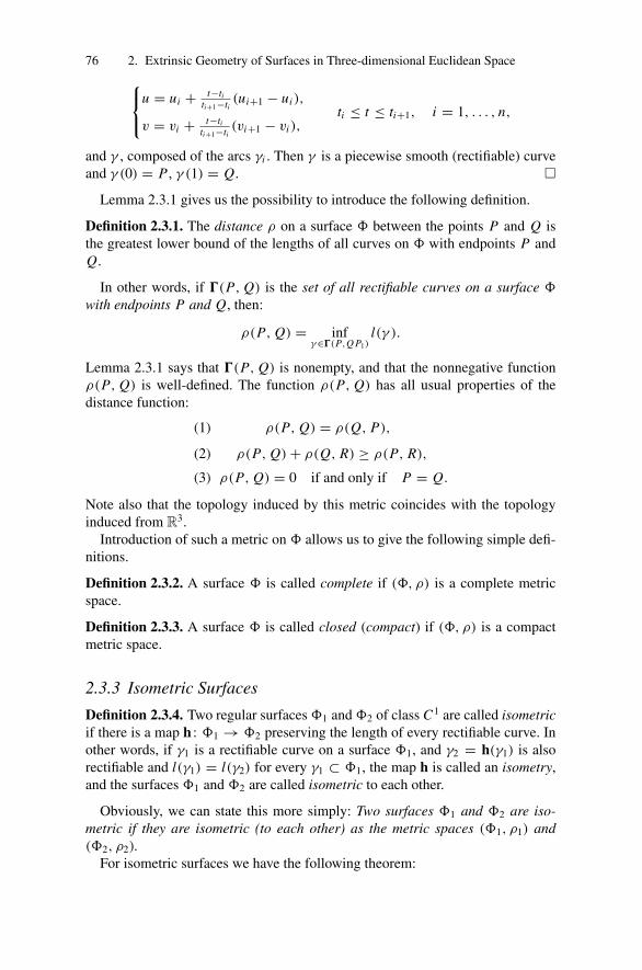
76 2. Extrinsic Geometry of Surfaces in Three-dimensional Euclidean Space⎧⎨⎩u = ui + t−titi+1−ti
(ui+1 − ui ),
v = vi + t−titi+1−ti
(vi+1 − vi ),ti ≤ t ≤ ti+1, i = 1, . . . , n,
and γ , composed of the arcs γi . Then γ is a piecewise smooth (rectifiable) curveand γ (0) = P , γ (1) = Q. �
Lemma 2.3.1 gives us the possibility to introduce the following definition.
Definition 2.3.1. The distance ρ on a surface � between the points P and Q isthe greatest lower bound of the lengths of all curves on � with endpoints P andQ.
In other words, if �(P, Q) is the set of all rectifiable curves on a surface �
with endpoints P and Q, then:
ρ(P, Q) = infγ∈�(P,Q P1)
l(γ ).
Lemma 2.3.1 says that �(P, Q) is nonempty, and that the nonnegative functionρ(P, Q) is well-defined. The function ρ(P, Q) has all usual properties of thedistance function:
(1) ρ(P, Q) = ρ(Q, P),
(2) ρ(P, Q) + ρ(Q, R) ≥ ρ(P, R),
(3) ρ(P, Q) = 0 if and only if P = Q.
Note also that the topology induced by this metric coincides with the topologyinduced from R3.
Introduction of such a metric on � allows us to give the following simple defi-nitions.
Definition 2.3.2. A surface � is called complete if (�, ρ) is a complete metricspace.
Definition 2.3.3. A surface � is called closed (compact) if (�, ρ) is a compactmetric space.
2.3.3 Isometric Surfaces
Definition 2.3.4. Two regular surfaces �1 and �2 of class C1 are called isometricif there is a map h : �1 → �2 preserving the length of every rectifiable curve. Inother words, if γ1 is a rectifiable curve on a surface �1, and γ2 = h(γ1) is alsorectifiable and l(γ1) = l(γ2) for every γ1 ⊂ �1, the map h is called an isometry,and the surfaces �1 and �2 are called isometric to each other.
Obviously, we can state this more simply: Two surfaces �1 and �2 are iso-metric if they are isometric (to each other) as the metric spaces (�1, ρ1) and(�2, ρ2).
For isometric surfaces we have the following theorem:
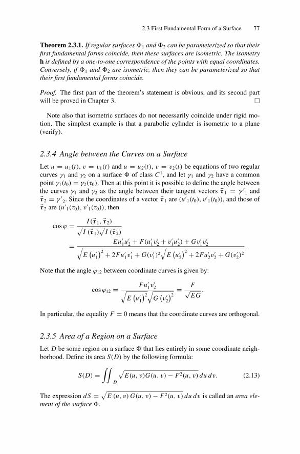
2.3 First Fundamental Form of a Surface 77
Theorem 2.3.1. If regular surfaces �1 and �2 can be parameterized so that theirfirst fundamental forms coincide, then these surfaces are isometric. The isometryh is defined by a one-to-one correspondence of the points with equal coordinates.Conversely, if �1 and �2 are isometric, then they can be parameterized so thattheir first fundamental forms coincide.
Proof. The first part of the theorem’s statement is obvious, and its second partwill be proved in Chapter 3. �
Note also that isometric surfaces do not necessarily coincide under rigid mo-tion. The simplest example is that a parabolic cylinder is isometric to a plane(verify).
2.3.4 Angle between the Curves on a Surface
Let u = u1(t), v = v1(t) and u = u2(t), v = v2(t) be equations of two regularcurves γ1 and γ2 on a surface � of class C1, and let γ1 and γ2 have a commonpoint γ1(t0) = γ2(τ0). Then at this point it is possible to define the angle betweenthe curves γ1 and γ2 as the angle between their tangent vectors �τ 1 = γ ′
1 and�τ 2 = γ ′
2. Since the coordinates of a vector �τ 1 are (u′1(t0), v′
1(t0)), and those of�τ 2 are (u′
1(τ0), v′1(τ0)), then
cos ϕ = I (�τ 1, �τ 2)√I (�τ 1)
√I (�τ 2)
= Eu′1u′
2 + F(u′1v
′2 + v′
1u′2) + Gv′
1v′2√
E(u′
1
)2 + 2Fu′1v
′1 + G(v′
1)2√
E(u′
2
)2 + 2Fu′2v
′2 + G(v′
2)2.
Note that the angle ϕ12 between coordinate curves is given by:
cos ϕ12 = Fu′1v
′2√
E(u′
1
)2√
G(v′
2
)2= F√
EG.
In particular, the equality F = 0 means that the coordinate curves are orthogonal.
2.3.5 Area of a Region on a Surface
Let D be some region on a surface � that lies entirely in some coordinate neigh-borhood. Define its area S(D) by the following formula:
S(D) =∫∫
D
√E(u, v)G(u, v) − F2(u, v) du dv. (2.13)
The expression d S = √E (u, v) G(u, v) − F2(u, v) du dv is called an area ele-
ment of the surface �.
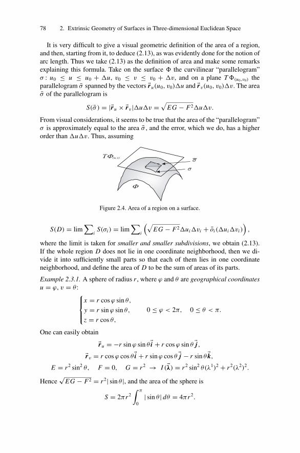
78 2. Extrinsic Geometry of Surfaces in Three-dimensional Euclidean Space
It is very difficult to give a visual geometric definition of the area of a region,and then, starting from it, to deduce (2.13), as was evidently done for the notion ofarc length. Thus we take (2.13) as the definition of area and make some remarksexplaining this formula. Take on the surface � the curvilinear “parallelogram”σ : u0 ≤ u ≤ u0 + �u, v0 ≤ v ≤ v0 + �v, and on a plane T �(u0,v0) theparallelogram σ spanned by the vectors �ru(u0, v0)�u and �rv(u0, v0)�v. The areaσ of the parallelogram is
S(σ ) = |�ru × �rv|�u�v =√
EG − F2�u�v.
From visual considerations, it seems to be true that the area of the “parallelogram”σ is approximately equal to the area σ , and the error, which we do, has a higherorder than �u�v. Thus, assuming
Figure 2.4. Area of a region on a surface.
S(D) = lim∑
iS(σi ) = lim
∑i
(√EG − F2�ui�vi + oi (�ui�vi )
),
where the limit is taken for smaller and smaller subdivisions, we obtain (2.13).If the whole region D does not lie in one coordinate neighborhood, then we di-vide it into sufficiently small parts so that each of them lies in one coordinateneighborhood, and define the area of D to be the sum of areas of its parts.
Example 2.3.1. A sphere of radius r , where ϕ and θ are geographical coordinatesu = ϕ, v = θ :⎧⎪⎨⎪⎩
x = r cos ϕ sin θ,
y = r sin ϕ sin θ,
z = r cos θ,
0 ≤ ϕ < 2π, 0 ≤ θ < π.
One can easily obtain
�ru = −r sin ϕ sin θ�i + r cos ϕ sin θ �j ,�rv = r cos ϕ cos θ�i + r sin ϕ cos θ �j − r sin θ �k,
E = r2 sin2 θ, F = 0, G = r2 → I (�λ) = r2 sin2 θ(λ1)2 + r2(λ2)2.
Hence√
EG − F2 = r2| sin θ |, and the area of the sphere is
S = 2πr2∫ π
0| sin θ | dθ = 4πr2.

2.4 Second Fundamental Form of a Surface 79
2.3.6 Formulas for Calculations
Surface given by the parametric equations. x = x(u, v), y = y(u, v), z =z(u, v).
E = x2u + y2
u + z2u, F = xu xv + yu yv + zuzv, G = x2
v + y2v + z2
v,
EG − F2 = (xu yv − xv yu)2 + (xuzv − xvzu)
2 + (yuzv − yvzu)2,
S =∫∫
D
√(xu yv − xv yu)2 + (xuzv − xvzu)2 + (yuzv − yvzu)2 du dv.
Explicitly given surface. z = f (x, y).
E = 1 + f 2x , F = fx fy, G = 1 + f 2
y , EG − F2 = 1 + f 2x + f 2
y ,
S =∫∫
D
√1 + f 2
x + f 2y dx dy.
2.4 Second Fundamental Form of a Surface
2.4.1 Normal curvature
Let P be some point on a regular surface � of class Ck (k ≥ 2). Consider theplane �(P, �λ) passing through a normal �n to � at P and a vector �λ ∈ T �P . Theintersection of this plane with � in some neighborhood of P is a regular curve γ
of class Ck (see Exercise 2.2.2).Denote by k(P, �λ) its curvature at P , and if k(P, �λ) �= 0, then denote
by �ν(P, �λ) the principal normal vector of γ at P . Since γ lies in the plane�(P, �λ), then �ν(P, �λ) = ±�n(P). Define the real number k(P, �λ) = 〈�ν(P, �λ),�n(P)〉k(P, �λ), i.e., assume that
k(P, �λ) =
⎧⎪⎨⎪⎩k(P, �λ) if �ν(P, �λ) = �n(P),
0 if k(P, �λ) = 0,
−k(P, �λ) if �ν(P, �λ) = −�n(P).
Definition 2.4.1. The normal curvature of a surface � at a point P and in thedirection �λ is the real number k(P, �λ).
Obviously, the sign of k(P, �λ) depends on the choice of the direction of thenormal �n(P), and it changes generally with varying this direction. Thus the signof k(P, �λ) itself has no geometric meaning. However, whether the sign varies orremains the same as the direction o f�λ changes does have geometric significance.So, if k(P, �λ) has constant sign for all �λ ∈ T �P , then � in some neighborhoodof P lies entirely on one side of its tangent plane T �P . But if k(P, �λ) changessign, then � lies on both sides of T �P . In the first case, the point P is said to
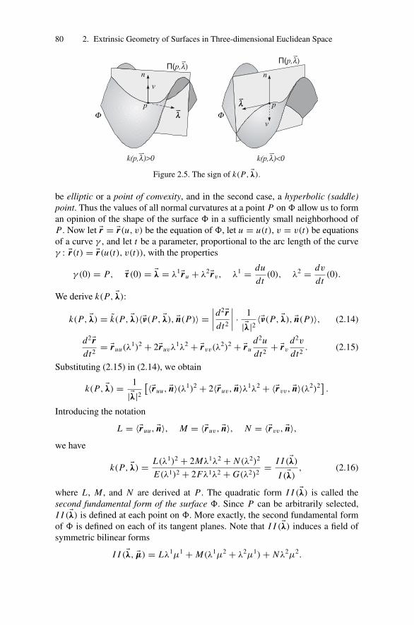
80 2. Extrinsic Geometry of Surfaces in Three-dimensional Euclidean Space
Figure 2.5. The sign of k(P, �λ).
be elliptic or a point of convexity, and in the second case, a hyperbolic (saddle)point. Thus the values of all normal curvatures at a point P on � allow us to forman opinion of the shape of the surface � in a sufficiently small neighborhood ofP . Now let �r = �r(u, v) be the equation of �, let u = u(t), v = v(t) be equationsof a curve γ , and let t be a parameter, proportional to the arc length of the curveγ : �r(t) = �r(u(t), v(t)), with the properties
γ (0) = P, �τ (0) = �λ = λ1�ru + λ2�rv, λ1 = du
dt(0), λ2 = dv
dt(0).
We derive k(P, �λ):
k(P, �λ) = k(P, �λ)〈�ν(P, �λ), �n(P)〉 =∣∣∣∣d2�r
dt2
∣∣∣∣ · 1
|�λ|2 〈�ν(P, �λ), �n(P)〉, (2.14)
d2�rdt2
= �ruu(λ1)2 + 2�ruvλ
1λ2 + �rvv(λ2)2 + �ru
d2u
dt2+ �rv
d2v
dt2. (2.15)
Substituting (2.15) in (2.14), we obtain
k(P, �λ) = 1
|�λ|2[〈�ruu, �n〉(λ1)2 + 2〈�ruv, �n〉λ1λ2 + 〈�rvv, �n〉(λ2)2
].
Introducing the notation
L = 〈�ruu, �n〉, M = 〈�ruv, �n〉, N = 〈�rvv, �n〉,we have
k(P, �λ) = L(λ1)2 + 2Mλ1λ2 + N (λ2)2
E(λ1)2 + 2Fλ1λ2 + G(λ2)2= I I (�λ)
I (�λ), (2.16)
where L , M , and N are derived at P . The quadratic form I I (�λ) is called thesecond fundamental form of the surface �. Since P can be arbitrarily selected,I I (�λ) is defined at each point on �. More exactly, the second fundamental formof � is defined on each of its tangent planes. Note that I I (�λ) induces a field ofsymmetric bilinear forms
I I (�λ, �µ) = Lλ1µ1 + M(λ1µ2 + λ2µ1) + Nλ2µ2.
2.4 Second Fundamental Form of a Surface 81
2.4.2 Formulas for Calculations
Surface given by the parametric equations. x = x(u, v), y = y(u, v), z =z(u, v):
L = 〈�ruu, �n〉 = (�ruu · �ru · �rv)
|�ru × �rv| = 1√EG − F2
∣∣∣∣∣∣xuu yuu zuu
xu yu zu
xv yv zv
∣∣∣∣∣∣ ,M = 〈�ruv, �n〉 = (�ruv · �ru · �rv)
|�ru × �rv| = 1√EG − F2
∣∣∣∣∣∣xuv yuv zuv
xu yu zu
xv yv zv
∣∣∣∣∣∣ ,N = 〈�rvv, �n〉 = (�rvv · �ru · �rv)
|�ru × �rv| = 1√EG − F2
∣∣∣∣∣∣xvv yvv zvv
xu yu zu
xv yv zv
∣∣∣∣∣∣ .Sometimes, for calculating L , M , and N it is more convenient to use the followingformulas:
L = −〈�ru, �nu〉, M = −〈�ru, �nv〉, N = −〈�rv, �nv〉, (2.17)
which are obtained from the previous formulas by differentiation of the identities
〈�ru, �n〉 = 0, 〈�rv, �n〉 = 0.
From (2.16) it is seen that the second fundamental form admits the invariant defi-nition
I I (�λ) = −⟨�λ,
d �nd�λ
⟩.
In classical notation, the second fundamental form is defined by the formula
I I (d�r) = −〈d�r, d �n〉,
where the direction d�r is defined by the ratio of differentials du : dv.
Explicitly given surface. z = f (x, y).
L = fxx√1 + f 2
x + f 2y
, M = fxy√1 + f 2
x + f 2y
, N = fyy√1 + f 2
x + f 2y
.
Example 2.4.1. We continue Example 2.3.1 with a sphere:
82 2. Extrinsic Geometry of Surfaces in Three-dimensional Euclidean Space
�ruu = −r cos ϕ sin θ�i − r sin ϕ sin θ �j ,�ruv = −r sin ϕ cos θ�i + r cos ϕ cos θ �j ,�rvv = −r cos ϕ sin θ�i − r sin ϕ sin θ �j − r cos θ �k,
L = −r sin ϕ(r2 sin2 ϕ sin2 θ + r2 cos2 ϕ sin2 θ)
2 sin θ= −r2 sin2 θ,
M = 0, N = −r2,
I I (�λ) = −r2[sin2 θ(λ1)2 + (λ2)2
].
Example 2.4.2. Cylinder:
⎧⎨⎩x = r cos v
y = r sin v
z = u, I I (�λ) = 1
r (λ1)2.
Example 2.4.3. Helicoid:
⎧⎨⎩x = u cos v
y = u sin v
z = cv, E = 1, F = 0, G = u2 + c2,
L = N = 0, M = c√u2 + c2
, I I (�λ) = c√u2 + c2
λ1λ2.
2.4.3 Meusnier’s Theorem
Let γ1 be an arbitrary C2-regular curve on a regular surface � of class C2 passingthrough the point P in the direction of the vector �λ. If a curvature k1 of γ1 at Pdiffers from zero, then denote by �ν1 the principal normal vector of γ1 at P . Definethe sign of curvature k1 analogously to previous considerations: the sign of k1 isassumed to be equal to the sign of 〈�ν1, �n(P)〉 if 〈�ν1, �n(P)〉 �= 0, and denote by θ
the angle between the vectors �n and �ν1.
Theorem 2.4.1 (Meusnier). The curvatures k1 and k(P, �λ) are related by theformula
k(P, �λ) = k1 · cos θ.
Proof. Let u = u1(t), v = v1(t) be equations of the curve γ1; let t be a parameterproportional to the arc length of γ1 : �r(t) = �r(u1(t), v1(t)) such that
γ 1(0) = P,du1
dt(0) = λ1,
dv1
dt(0) = λ2, �λ = λ1�ru + λ2�rv.
Since
d2�rdt2
= �ruu(λ1)2 + 2�ruvλ
1λ2 + �rvv(λ2)2 + �ru
d2u
dt2+ �rv
d2v
dt2,
then
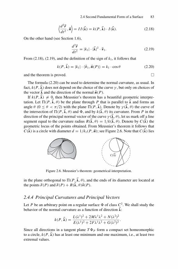
2.4 Second Fundamental Form of a Surface 83
⟨d2�rdt2
, �n⟩= I I (�λ) = k(P, �λ) · I (�λ). (2.18)
On the other hand (see Section 1.6),
d2�rdt2
= |k1| · |�λ|2 · �ν1. (2.19)
From (2.18), (2.19), and the definition of the sign of k1, it follows that
k(P, �λ) = |k1| · 〈�ν1, �n(P)〉 = k1 · cos θ (2.20)
and the theorem is proved. �
The formula (2.20) can be used to determine the normal curvature, as usual. Infact, k(P, �λ) does not depend on the choice of the curve γ , but only on choices ofthe vector �λ and the direction of the normal �n(P).
If k(P, �λ) �= 0, then Meusnier’s theorem has a beautiful geometric interpre-tation. Let �(P, �λ, θ) be the plane through P that is parallel to �λ and forms anangle θ (0 ≤ θ < π/2) with the plane �(P, �λ). Denote by γ (�λ, θ) the curve ofthe intersection of �(P, �λ, θ) and �, and by k(�λ, θ) its curvature. From P in thedirection of the principal normal vector of the curve γ (�λ, θ), let us mark off a linesegment equal to the curvature radius R(�λ, θ) = 1/k(�λ, θ). Denote by C(�λ) thegeometric locus of the points obtained. From Meusnier’s theorem it follows thatC(�λ) is a circle with diameter d = 1/k1(P, �n); see Figure 2.6. Note that C(�λ) lies
Figure 2.6. Meusnier’s theorem: geometrical interpretation.
in the plane orthogonal to �(P, �λ, θ), and the ends of its diameter are located atthe points �r(P) and �r(P) + R(�λ, θ)�ν(P).
2.4.4 Principal Curvatures and Principal Vectors
Let P be an arbitrary point on a regular surface � of class C2. We shall study thebehavior of the normal curvature as a function of direction �λ:
k(P, �λ) = L(λ1)2 + 2Mλ1λ2 + N (λ2)2
E(λ1)2 + 2Fλ1λ2 + G(λ2)2.
Since all directions in a tangent plane T �P form a compact set homeomorphicto a circle, k(P, �λ) has at least one minimum and one maximum, i.e., at least twoextremal values.

84 2. Extrinsic Geometry of Surfaces in Three-dimensional Euclidean Space
Definition 2.4.2. A principal curvature of a surface � at a point P is an extremalvalue of a normal curvature function k(P, �λ) at a given point P on �. The direc-tions (vectors) in T �P for which k(P, �λ) takes its extremal values are principalvectors of the surface � at the point P .
We now derive the equations for deriving the principal curvatures and the prin-cipal vectors. Let a0 be a principal curvature, �λ0 the corresponding principal vec-tor, �λ0 = λ1
0�ru +λ20�rv , and �λ = λ1�ru +λ2�rv an arbitrary vector in the plane T �P .
Then the function
f (λ1, λ2, a0) = I I (�λ) − a0 · I (�λ)
and its derivatives ∂ f /∂λ1 and ∂ f /∂λ2 take zero values for λ1 = λ10, λ2 = λ2
0. Inthis way, we obtain the following system of equations:⎧⎨⎩
I I (�λ0) − a0 · I (�λ0) = 0,
I Iλ1(�λ0) − a0 · Iλ1(�λ0) = 0,
I Iλ2(�λ0) − a0 · Iλ2(�λ0) = 0,
(2.21)
or, in more detailed form,{(L − a0 E)λ1
0 + (M − a0 F)λ20 = 0
(M − a0 F)λ10 + (N − a0G)λ2
0 = 0.(2.22)
Since �λ0 �= 0, the system (2.22) has nonzero solution λ10, λ
20, and hence∣∣∣∣ L − a0 E M − a0 F
M − a0 F N − a0G
∣∣∣∣ = 0,
or
(EG − F2)a20 − (E N + GL − 2M F)a0 + L N − M2 = 0. (2.23)
Thus, we see that there exist not more than two principal curvatures. But if (2.23)has a unique solution, then min�λ k(P, �λ) = max�λ k(P, �λ), and k(P, �λ) does notdepend on �λ. In this case any �λ ∈ T �P is a principal vector. Denote by k1(P) andk2(P) the principal curvatures of the surface � at the point P; k1(P) ≤ k2(P).We now deduce the equation for deriving the principal vectors. The system (2.21)has nonzero solution (1, −a0). Thus
I Iλ1(�λ0) · Iλ2(�λ0) − I Iλ2(�λ0) · Iλ1(�λ0) = 0,
or in more detailed form,
(Eλ10 + Fλ2
0)(Mλ10 + Nλ2
0) − (Fλ10 + Gλ2
0)(Lλ10 + Mλ2
0) = 0.
The last equation can be written in a form more convenient for applications andmemorization:
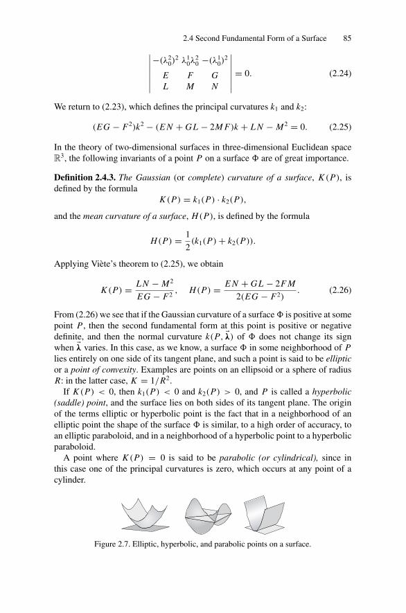
2.4 Second Fundamental Form of a Surface 85∣∣∣∣∣∣∣−(λ2
0)2 λ1
0λ20 −(λ1
0)2
E F GL M N
∣∣∣∣∣∣∣ = 0. (2.24)
We return to (2.23), which defines the principal curvatures k1 and k2:
(EG − F2)k2 − (E N + GL − 2M F)k + L N − M2 = 0. (2.25)
In the theory of two-dimensional surfaces in three-dimensional Euclidean spaceR3, the following invariants of a point P on a surface � are of great importance.
Definition 2.4.3. The Gaussian (or complete) curvature of a surface, K (P), isdefined by the formula
K (P) = k1(P) · k2(P),
and the mean curvature of a surface, H(P), is defined by the formula
H(P) = 1
2(k1(P) + k2(P)).
Applying Viete’s theorem to (2.25), we obtain
K (P) = L N − M2
EG − F2, H(P) = E N + GL − 2F M
2(EG − F2). (2.26)
From (2.26) we see that if the Gaussian curvature of a surface � is positive at somepoint P , then the second fundamental form at this point is positive or negativedefinite, and then the normal curvature k(P, �λ) of � does not change its signwhen �λ varies. In this case, as we know, a surface � in some neighborhood of Plies entirely on one side of its tangent plane, and such a point is said to be ellipticor a point of convexity. Examples are points on an ellipsoid or a sphere of radiusR: in the latter case, K = 1/R2.
If K (P) < 0, then k1(P) < 0 and k2(P) > 0, and P is called a hyperbolic(saddle) point, and the surface lies on both sides of its tangent plane. The originof the terms elliptic or hyperbolic point is the fact that in a neighborhood of anelliptic point the shape of the surface � is similar, to a high order of accuracy, toan elliptic paraboloid, and in a neighborhood of a hyperbolic point to a hyperbolicparaboloid.
A point where K (P) = 0 is said to be parabolic (or cylindrical), since inthis case one of the principal curvatures is zero, which occurs at any point of acylinder.
Figure 2.7. Elliptic, hyperbolic, and parabolic points on a surface.

86 2. Extrinsic Geometry of Surfaces in Three-dimensional Euclidean Space
The mean curvature of a surface plays a less important role in the theory ofsurfaces than Gaussian curvature. We make only one remark.
A surface � is minimal if the mean curvature vanishes at all points of �.A minimal surface is characterized locally by the property of having minimal
area among all surfaces with the same boundary contour.
2.4.5 Umbilics
Definition 2.4.4. A point P on a surface � is called an umbilical point or umbilicif the principal curvatures k1(P) and k2(P) are equal. If in addition the equalityk1(P) = k2(P) = 0 holds, then P is called a planar point.
The notion of these points is explained by the fact that on a sphere of radius Rthe equality k1(P) = k2(P) = ±1/R holds at every point P , and at every pointon a plane, k1(P) = k2(P) = 0 holds. Later, we shall prove a theorem that if allpoints on a surface � are umbilics, then � is a (open) domain of a sphere or aplane.
The normal curvature at an umbilic does not depend on the direction, and thusthe second fundamental form is proportional to the first fundamental form, andthe coefficient of proportionality is the principal curvature of the surface � at thispoint: L = k E , M = k F , N = kG, where k = k1 = k2. The opposite is also true:if L
E = MF = N
G , then P is an umbilic.By the way, we have obtained the following theorem.
Theorem 2.4.2. A point P on a regular surface � of class Ck (k ≥ 2) is umbilicif and only if the equalities L
E = MF = N
G hold, and P is a planar point if and onlyif the equalities L = M = N = 0 hold.
It can be shown that a connected surface consisting only of umbilical points ispart of a sphere. The general ellipsoid has four umbilics; see also Problem 2.7.2.The Caratheodory conjecture that a surface homeomorphic to a sphere has atleast two umbilics is still open.5
2.4.6 Orthogonality of Principal Vectors
If a point P on a surface � is not umbilic, then there exist exactly two principalvectors in the tangent plane T �P . It turns out that these directions are mutuallyorthogonal, and adjoint with respect to the second fundamental form.
Theorem 2.4.3. If a point P on a regular surface � is not umbilic, and twovectors �λ1, �λ2 ∈ T �P are parallel to the principal vectors of � at P, thenI (�λ1, �λ2) = I I (�λ1, �λ2) = 0.
5 A recent survey about umbilics on surfaces is Gutierrez, C. and Sotomayor, J., Lines of curvature,umbilic points and Caratheodory conjecture. Resen. Inst. Mat. Estat. Univ. Sao Paulo, Vol. 3, No.3, 291–322, 1998. The proof for the analytical case can be found in Ivanov, V.V., The analyticconjecture of Caratheodory, Siberian Math. J., v. 43, 251–322, 2002.

2.4 Second Fundamental Form of a Surface 87
Proof. We write down (2.21), which defines the principal vectors:⎧⎨⎩I Iλ11(�λ1) − k1 · Iλ1
1(�λ1) = 0,
I Iλ21(�λ1) − k1 · Iλ2
1(�λ1) = 0,
(2.27)
⎧⎨⎩I Iλ12(�λ2) − k2 · Iλ1
2(�λ2) = 0,
I Iλ22(�λ2) − k2 · Iλ2
2(�λ2) = 0.
(2.28)
Multiplying the first equation of system (2.27) by λ12 and the second equation by
λ22 and summing them, we obtain
2 · I I (�λ1, �λ2) − 2k1 · I (�λ1, �λ2) = 0. (2.29)
Analogously, multiplying the first equation of system (2.28) by λ11 and the second
equation by λ21 and summing them, we obtain
2 · I I (�λ1, �λ2) − 2k2 · I (�λ1, �λ2) = 0. (2.30)
Now subtracting (2.30) from (2.29), and by taking into account that k2 − k1 �= 0,we obtain
I (�λ1, �λ2) = 〈�λ1, �λ2〉 = 0. (2.31)
From (2.29) and (2.31) follows I I (�λ1, �λ2) = 0. �
2.4.7 Euler’s Formula
A formula first deduced by Euler allows us to derive the normal curvature of asurface � at a given point P and in an arbitrary direction from the known principalcurvatures k1 and k2 of the surface at this point. Denote by �λ1 = λ1
1�ru + λ21�rv and
�λ2 = λ12�ru + λ2
2�rv two mutually orthogonal unit vectors going along the principaldirections. The existence of such vectors follows from Theorem 2.4.3 and theremark before Theorem 2.4.2. Denote by �λ(ϕ) the vector that forms an angle ϕ
(0 ≤ ϕ ≤ 2π) with �λ1.
Theorem 2.4.4. For an arbitrary point P on a regular surface � of class Ck
(k ≥ 2), the following equality (called Euler’s formula) holds:
k(P, ϕ) = k(P, �λ(ϕ)) = k1 cos2 ϕ + k2 sin2 ϕ.
Proof. Introduce a coordinate system (u, v) in a neighborhood of P such thatP(0, 0) and �ru(0, 0) = �λ1, �rv(0, 0) = �λ2. The existence of such coordinatesfollows from Lemma 2.1.2. In this coordinate system we have
λ11 = 1, λ2
1 = 0, λ12 = 0, λ2
2 = 1, λ1(ϕ) = cos ϕ, λ2(ϕ) = sin ϕ,
E(0, 0) = G(0, 0) = 1, F(0, 0) = M(0, 0) = 0.

88 2. Extrinsic Geometry of Surfaces in Three-dimensional Euclidean Space
All these equalities follow from the definition of E , F , G, but the last equalityfollows from Theorem 2.4.3, since I I (�λ1, �λ2) = M = 0. Furthermore,
k(P, ϕ) = L cos2 ϕ + N sin2 ϕ
cos2 ϕ + sin2 ϕ= L cos2 ϕ + N sin2 ϕ.
On the other hand,
k1 = k(P, 0) = L , k2 = k(
P,π
2
)= N .
Thus we obtain k(P, ϕ) = k1 cos2 ϕ + k2 sin2 ϕ. �
2.4.8 Rodrigues’s Theorem
Theorem 2.4.5 (Rodrigues). The derivative of a normal �n(P) to a regular sur-face � of class Ck (k ≥ 2) along some direction is parallel to it if and only ifthis direction is the principal vector of the surface at P and the coefficient ofproportionality is equal to −k, where k is the principal curvature of � at P cor-responding to this principal vector.
Proof. Let �λ = λ1�ru + λ2�rv be the vector that defines the direction under discus-sion. The derivative of the vector field �n(P) along the direction �λ, in view of thedefinition of directional derivative, is written in the following form:
d �nd�λ = λ1�nu + λ2�nv. (2.32)
Let �λ be a principal vector. Then by Theorem 2.4.3, there is a vector �µ = µ1�ru +µ2�rv such that the following equalities are satisfied:
I (�λ, �µ) = I I (�λ, �µ) = 0.
The scalar product of (2.32) by the vector �µ gives us⟨d �nd�λ , �µ
⟩= −I I (�λ, �µ) = 0. (2.33)
Consequently, d �nd�λ is orthogonal to the vector �µ. Hence it is collinear with �λ, and
we have d �nd�λ = a�λ. We now find the value of a. The scalar product of the last
equation by the vector �λ gives us −I I (�λ) = a · I (�λ), or a = − I I (�λ)
I (�λ)= −k. Now
let the equality
d �nd�λ = a�λ (2.34)
be given. As before, we obtain a = −k, and it remains to prove only that �λ isparallel to the principal vector. From (2.32) and (2.34) follows the equality
2.4 Second Fundamental Form of a Surface 89
λ1�nu + λ2�nv = (λ1�ru + λ2�rv)(−k).
Its scalar product, first by �ru , and then by �rv , gives us a system of equations{−Lλ1 − Mλ2 = −k Eλ1 − k Fλ2,
−Mλ1 − Nλ2 = −k Fλ1 − kGλ2,
which coincides with the system (2.22), and hence �λ is a principal vector. Thetheorem is proved. �
Consider one application of Rodrigues’s theorem. Solve the following problem.
Problem 2.4.1. If the normal curvature k(P, �λ) of a regular surface � of class Ck
(k ≥ 3) depends on neither P nor �λ, then � is an open connected domain oneither a sphere or a plane.
Solution. Take an arbitrary point P ∈ �. Select the direction of a normal �n at Pand on some neighborhood in such a way that the normal curvatures of the surfaceare positive; i.e., assume that k(P, �λ) ≡ k0 > 0. Take an arbitrary direction�λ ∈ T �P and denote by �(P, �λ) the plane through a point P that is parallel tothe vectors �n and �λ, and by γ (P, �λ) the curve that appears as the intersection of �
and a plane �(P, �λ). Introduce on γ (P, �λ) the arc length parameterization witht counting from the point P . Denote by �τ (t), �ν(t), and �β(t) a tangent vector, theprincipal normal vector and the binormal of γ (P, �λ). The curve γ (P, �λ) is a planecurve, and its torsion is zero. Thus from the Frenet formulas (see Section 1.9) weobtain
�τ ′(t) = k�ν(t), �ν ′
(t) = −k�τ (t), �β ′(t) = 0, (2.35)
where k(t) is the curvature of γ (P, �λ). On the other hand, from Rodrigues’s the-orem we have
�n′(t) = −k0�τ (t). (2.36)
Set �a(t) = �n(t) − �ν(t). Then �a(0) = 0, and since �a(t) is orthogonal to �τ (t), then
�a(t) = c1(t)�β(t) + c2(t)�ν(t), (2.37)
where c1(t) and c2(t) are some differentiable functions. Thus, on the one hand,we have
d�adt
= d �ndt
− d�νdt
= (k − k0)�τ , (2.38)
but on the other hand,
d�adt
= c′1(t)�β + c′
2(t)�ν + c2(t)(−k�τ ). (2.39)
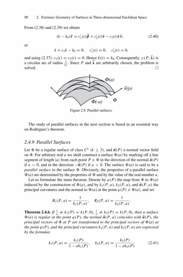
90 2. Extrinsic Geometry of Surfaces in Three-dimensional Euclidean Space
From (2.38) and (2.39) we obtain
(k − k0)�τ = c′1(t)�β + c′
2(t)�ν − c2(t)k�τ , (2.40)
ork + c2k − k0 = 0, c′
1(t) = 0, c′2(t) = 0,
and using (2.37): c1(t) = c2(t) = 0. Hence k(t) = k0. Consequently, γ (P, �λ) isa circular arc of radius 1
k0. Since P and �λ are arbitrarily chosen, the problem is
solved. �
Figure 2.8. Parallel surfaces.
The study of parallel surfaces in the next section is based in an essential wayon Rodrigues’s theorem.
2.4.9 Parallel Surfaces
Let � be a regular surface of class Ck (k ≥ 3), and �n(P) a normal vector fieldon �. For arbitrary real a we shall construct a surface �(a) by marking off a linesegment of length |a| from each point P ∈ � in the direction of the normal �n(P)
if a > 0, and in the direction −�n(P) if a < 0. The surface �(a) is said to be aparallel surface to the surface �. Obviously, the properties of a parallel surface�(a) are determined by the properties of � and by the value of the real number a.
Let us formulate the main theorem. Denote by ϕ(P) the map from � to �(a)
induced by the construction of �(a), and by k1(P, a), k2(P, a), and �n(P, a) theprincipal curvatures and the normal to �(a) at the point ϕ(P) ∈ �(a), and set
R1(P, a) = 1
k1(P, a), R2(P, a) = 1
k2(P, a).
Theorem 2.4.6. If 1a �= k1(P) = k(P, 0), 1
a �= k2(P) = k(P, 0), then a surface�(a) is regular at the point ϕ(P), the normal �n(P, a) coincides with �n(P), theprincipal vectors of � at P are transformed to the principal vectors of �(a) atthe point ϕ(P), and the principal curvatures k1(P, a) and k2(P, a) are expressedby the formulas
k1(P, a) = k1(P)
1 − ak1(P), k2(P, a) = k2(P)
1 − ak2(P)(2.41)
2.5 The Third Fundamental Form of a Surface 91
or
R1(P, a) = R1(P) − a, R2(P, a) = R2(P) − a. (2.42)
Proof. Introduce a parameterization �r = �ρ(u, v) of the surface � in a neigh-borhood of P such that P has nonzero coordinates and the vectors �ρu(0, 0) and�ρv(0, 0) are parallel to the principal vectors of � at P . The equation of the surface�(a) can be written as
�r = �r(u, v) = �ρ(u, v) + a�n(u, v).
We derive �ru × �rv at P
�ru = �ρu + a�nu, �rv = �ρv + a�nv.
From Rodrigues’s theorem it follows that
�ru = (1 − ak1)�ρu, �rv = (1 − ak2)�ρv. (2.43)
From (2.43) and the conditions of the theorem we have
�ru × �rv = (1 − ak1)(1 − ak2)[�ρu × �ρv] �= 0.
From the last formula, the first and second statements of the theorem follow. Fur-thermore, by Rodrigues’s theorem,
(�n(P, a))u = �nu = −k1 �ρu, (�n(P, a))v = �nv = −k2 �ρv.
From this and from (2.43) we obtain
(�n(P, a))u = −k1
1 − ak1�ru, (�n(P, a))v = −k2
1 − ak2�rv. (2.44)
From (2.44) and Rodrigues’s theorem we obtain
−k1(P, a)�ru = −k1
1 − ak1�ru, −k2(P, a)�rv = −k2
1 − ak2�rv. �
2.5 The Third Fundamental Form of a Surface
On a regular surface � of class Ck (k ≥ 3) one more fundamental form can bedefined: the third fundamental form. Let �λ = λ1�ru + λ2�rv be an arbitrary vector.Then suppose
I I I (�λ) =⟨
d �nd�λ ,
d �nd�λ
⟩= 〈λ1�nu+λ2�nv, λ1�nu+λ2�nv〉 = e(λ1)2+2 f λ1λ2+g(λ2)2,
where e = 〈�nu, �nu〉, f = 〈�nu, �nv〉, g = 〈�nv, �nv〉.Note that I I I (�λ) induces a field of symmetric bilinear forms
I I I (�λ, �µ) = eλ1µ1 + f (λ1µ2 + λ2µ1) + gλ2µ2.
It turns out that the three fundamental forms of a surface are linearly dependent.

92 2. Extrinsic Geometry of Surfaces in Three-dimensional Euclidean Space
Theorem 2.5.1. At each point on a regular surface � of class Ck (k ≥ 3) thefollowing equality holds:
K · I (�λ) − 2H · I I (�λ) + I I I (�λ) = 0. (2.45)
Recall that K (P) is the Gaussian curvature of the surface at P , and H(P) themean curvature.
Proof. Let P be an arbitrary point on �. Introduce coordinates (u, v) in someneighborhood of this point such that the vectors �ru and �rv at P become parallelto the principal vectors. Then from Rodrigues’s theorem and Theorem 2.4.3 weobtain, at the point P ,
〈�ru, �rv〉 = 0, (2.46)
�nu = −k1�ru, �nv = −k2�rv. (2.47)
From (2.46) and (2.47) follow
I (�λ) = E(λ1)2 + G(λ2)2,
I I (�λ) = −⟨�λ,
d �nd�λ
⟩= k1 E(λ1)2 + k2G(λ2)2, (2.48)
I I I (�λ) =⟨
d �nd�λ ,
d �nd�λ
⟩= k2
1 E(λ1)2 + k22 G(λ2)2.
From (2.48) we obtain
K · I (�λ) − 2H · I I (�λ) + I I I (�λ)
= k1k2[E(λ1)2 + G(λ2)2
]− (k1 + k2)
[k1 E(λ1)2 + k2G(λ2)2 + k2
1 E(λ1)2 + k22 G(λ2)2
]= E(λ1)2[k1k2 − k1(k1 + k2) + k2
1]+ G(λ2)2[k1k2 − k2(k1 + k2) + k2
2] = 0. �
Remark 2.5.1. The equality (2.45) was proved for a special coordinate system,but since all characteristics in (2.45) are invariant, the equality is valid in anycoordinate system. We write down (2.45) in more detailed form for an arbitrarycoordinate system:
K E − 2H L + e = 0, K F − 2H M + f = 0, K G − 2H N + g = 0. (2.49)
From (2.45) it follows that the third fundamental form of a surface does not itselfplay an essential role in the theory of surfaces. However, (2.45) or the equalities(2.49) may be useful for solving some interesting problems.
We shall give one example where the equalities (2.49) are used for provingGauss’s theorem about the area of a spherical image. Let us introduce two newnotions.

2.5 The Third Fundamental Form of a Surface 93
Definition 2.5.1. Let D be some region on a regular surface � of class C2. Toeach point on this surface we associate a point on the sphere S2(1) of unit radiusby the following rule. Take a normal �n(P) to � at a point P , and translate it byparallel displacement until the origin of the vector �n(P) coincides with the centerof the sphere S2(1). Then the endpoint of �n(P) will coincide with some pointϕ(P) on S2(1). The map ϕ(P) : D → S2(1) thus constructed is called a Gauss(spherical) map of the region D on the surface �.
Figure 2.9. Gauss (spherical) map.
Definition 2.5.2. If D is some region on a surface �, then the real numberω(D) = ∫∫
D K d S is called the integral curvature of D. If D lies entirely insome coordinate neighborhood (u, v), then
ω(D) =∫∫
DK (u, v)
√E(u, v)G(u, v) − F2(u, v) du dv. (2.50)
Example 2.5.1. The Gauss (spherical) map of a sphere is a similarity. The spher-ical image of a cylindrical surface is a part of a great circle (i.e., an intersectionwith a plane containing the center of the sphere) on S2(1). The spherical image ofa plane is a point.
Assume now that some region D on the surface � is in one-to-one correspon-dence with some region D∗ = ϕ(D) under the Gauss (spherical) map, and theGaussian curvature of � has the same sign at each point of D. Then the followingtheorem holds.
Theorem 2.5.2 (Gauss theorem for a spherical map). The modulus of the inte-gral curvature of a region D is equal to the area of its spherical image
|ω(D)| =∫∫
D∗d S1, (2.51)
where d S1 is an area element on a sphere.
Proof. Without loss of generality, assume that D lies inside a coordinate neigh-borhood; otherwise, divide it into parts, each of which lies in some coordinateneighborhood. Then prove the theorem separately for each such point and, inview of the additive nature of (2.51), deduce it for the entire region. Under thisassumption the map ϕ is determined by the formula �r = �r1(u, v) = �n(u, v).
94 2. Extrinsic Geometry of Surfaces in Three-dimensional Euclidean Space
Consequently, for this parameterization the first fundamental form of a spherecoincides with the third fundamental form of �. But then
S(D∗) =∫∫
D∗
√e(u, v)g(u, v) − f 2(u, v) du dv. (2.52)
We find√
eg − f 2, using (2.49), that
eg − f 2 = (2H L − K E)(2H N − K G) − (2H M − K F)2
= K 2(EG − F2) − 2H K (LG − E N − 2M F) + 4H 2(L N − M2)
= K 2(EG − F2) − 2H K · 2H(EG − F2) + 4H 2 · K (EG − F2)
= K 2(EG − F2).
Consequently,
S(D∗) =∫∫
D
√eg − f 2 du dv =
∫∫D
|K |√
EG − F2 du dv = |ω(D)|. �
Corollary 2.5.1. The ratio of the area of a spherical image of a region on a surfaceto the area of this region tends to the modulus of the Gaussian curvature at a givenpoint P when a region ties up to this point and K (P) �= 0.
Proof. If the Gaussian curvature at P differs from zero, then there is a neigh-borhood of P in which the Gaussian curvature has a fixed sign, and a Gauss(spherical) map of this region onto a sphere is single-valued. Then
S(D∗)S(D)
= ω(D)
S(D)= | ∫∫ D K d S|
S(D)= |K (Q)| ∫∫ D d S∫∫
D d S= |K (Q)|,
where Q is some point in our region. If a region ties up to a point P , then Q → P;thus lim S(D∗)
S(D)= |K (P)|. �
The Gauss theorem on the area of a spherical image has a perspective gener-alization. It is possible to add a clear geometrical sense to the formula (2.51):without the requirement of single-valuedness of a Gauss (spherical) map and con-stancy of the sign of Gaussian curvature, it can be written in the following form:
ω(D) =∫∫
DK d S =
∫∫D∗
d S1.
To prove this formula and give it a geometric meaning, one needs a generalizationof a notion of the area of a spherical image, which we omit for lack of space.
An application of the Gauss theorem on the area of a spherical image:Let O be some point in R3. Denote by P(O) the set of all orientable planes in
the space R3 passing through the point O . The set P(O) can be parameterized bythe points of the unit sphere S1(O) with center at the point O , by corresponding
2.6 Classes of Surfaces 95
to each point Q ∈ S1(O) a pair: a plane α through the point O that is orthogonalto the vector
−→O Q, and the vector
−→O Q itself. Obviously, this map has an inverse.
Now let � be a regular surface of class Ck (k ≥ 2). Denote by P(�, O) asubset of all orientable planes of the set P(O), for which the function fα(P) hasat least one degenerate critical point on �.
Problem 2.5.1. Prove that the set P(�, O) is nowhere dense in the set P(O)
relative to the topology of the sphere S1(O).
Hint. Sketch of solution: It is not difficult to check that the point P0 on � is adegenerate critical point of the function fα(P) if and only if T �P belongs to theset P(�, O). Now, using Gauss’s theorem on spherical images, we see that theset P(�, O) has zero measure on the sphere S1(O). From this, the statement ofthe problem is deduced.
Problem 2.5.2. If the Gaussian curvature of a closed surface � is positive, then|ω(�)| = 4π .
2.6 Classes of Surfaces
Before starting with the material of this section, let us return to a discussion of thenotion of a surface. The problem is that the definition given previously is rathercoarse; it excludes the surfaces with points of self-intersection, but such surfacesoften arise in natural geometric constructions, for instance, in the construction ofparallel surfaces.
A surface in the sense of Definition 2.1.1 is an embedded surface; the termtwo-dimensional manifold embedded in R3 is also used. We introduce now a newclass of surfaces: the immersed surfaces.
Definition 2.6.1. A set � is the immersed surface in R3 if there is an embeddedsurface � and a map ϕ : � → � that is a local diffeomorphism.
The difference between embedded and immersed surfaces is not essential whenwe study the local properties of a surface. Indeed, if a point P on an immersedsurface � is a point of self-intersection, then we take the points P1 and P2 on �
that are inverse images of P under the map ϕ. Select on the surface � the coor-dinate neighborhoods W1 and W2 of these points, each taken sufficiently small sothat W1 ∩ W2 = ∅ holds. Define W1 = ϕ(W1) and W2 = ϕ(W2).
Thus P has two coordinate neighborhoods on �: a neighborhood W1 on one“leaf” of a surface � and a neighborhood W2 on a second “leaf ,” and local studyof geometrical properties of � is reduced to local study of geometrical propertiesof first and second “leaves” separately. It turns out that at a given point P ∈ � weobtain two collections of geometric characteristics, which correspond to first andsecond “leaf ,” for instance, two values of the Gaussian curvature or two tangentplanes. Thus, for local investigation of immersed surfaces, it is more convenient to
96 2. Extrinsic Geometry of Surfaces in Three-dimensional Euclidean Space
imagine a point of self-intersection as two different points. Indeed, it may happenthat there are not two, but three or more, “leaves” through a given point P ∈ �.
During the study of the properties of surfaces in the large the difference be-tween immersed and embedded surfaces can be essential. However, in most cases,a fact that holds for embedded surfaces is also true for immersed surfaces, but theproof in the latter case is often substantially more difficult.
We shall give one more notion that is useful for solving problems “in the large.”
Definition 2.6.2. An immersion of a two-dimensional manifold (surface) � intoR3 is called proper if the intersection of any compact subset of the space R3 with� is compact with respect to the intrinsic metric on �.
2.6.1 Surfaces of Revolution
Let a curve γ lie in the plane (x, z) and let its equation have the form z = f (x).Assume that the function f (x) ∈ C2 is monotonic — for simplicity, stronglymonotonic. Denote by � the surface obtained by a rotation of γ about the axisO Z . The equation of this surface can be written in the following form:
z = f (√
x2 + y2) = f (r), r =√
x2 + y2.
Using the formulas of Section 2.3, we find that
E = 1 +( x
rf ′)2
, G = 1 +( y
rf ′)2
, F = xy
r2( f ′)2, EG − F2 = 1 + ( f ′)2.
Since our surface is a surface of revolution, it is sufficient to find these geometricalcharacteristics at the points on some meridian of the surface, say y = 0. For pointsof this meridian, F = 0, G = 1, and E = 1 + (
f ′)2hold. For the coefficients
L , M, N of the second fundamental form we obtain
L = f ′′√1 + ( f ′)2
, M = 0, N = f ′
x√
1 + ( f ′)2,
if a normal �n(P) of a surface � is directed from the axis O Z of rotation. Hence,the Gaussian curvature is
K = f ′′ f ′
x[1 + ( f ′)2]2.
From visual observations it follows that K must be negative if the convexity ofγ is directed along the axis O Z , and positive in the opposite case. In fact, if theconvexity of γ is directed along the axis O Z , then d2z
dx2 > 0, but d2zdx2 = − f ′′
( f ′)3 .Consequently, − f ′′ f ′ > 0 or − f ′′ f ′ < 0, and in the second case, − f ′′ f ′ < 0 or− f ′′ f ′ > 0; and since x > 0, our computations confirm the visual observations.
We now find the principal vectors and the principal curvatures. Hence the di-rections that are tangent to the meridian and parallels are the principal vectors.Moreover, from (2.25) we obtain

2.6 Classes of Surfaces 97
k1 = L
E= f ′′
[1 + ( f ′)2]3/2, k2 = N
G= f ′
x√
1 + ( f ′)2.
So, we see that k1 is simply the curvature of γ , and the sign of k1 is defined by thesign of f ′′.
We now clear up the geometrical sense of the principal curvature k2. Draw astraight line through a point P(x, f (x)), which is orthogonal to the curve γ . Theequation of this straight line is written as (X − x) + f ′(x)(Z − f (x)) = 0, whereX and Z are coordinates of a point on the straight line. We find the intersectionof this straight line with the axis O Z . The point Q of intersection has coordinatesx = 0, z = (x + f f ′)/ f ′. Denote by R the distance between P and Q and obtain
R =√
x2 +(
x + f f ′
f ′ − f
)2
= x√
1 + ( f ′)2
| f ′| .
Consequently, |k2| = 1/R.
Remark 2.6.1. For a surface of revolution there often exists such a parameteriza-tion �r(u, v) such that the coefficients of the first fundamental form are expressedas E = 1, F = 0, G = G(u). In fact, if the parameter u is taken equal to√
x2 + y2, and v equal to the rotation angle of the plane X O Z around the axisO Z , then
x = u cos v, y = u sin v, z = f (u)
are actually the parametric equations of our surface of revolution �. For this pa-rameterization we have
�ru = cos v�i + sin v�j + f ′ �k, �rv = −u sin v�i + u cos v�j .Thus
E = 1 + ( f ′)2, F = 0, G = u2.
We introduce a new parameter
u(u) =∫ u
u0
√1 + ( f ′)2 du
and let u = H(u) be the inverse function. Then �r u = �ru H ′, and hence we obtain
E = (�r u)2 = [
1 + ( f ′)2](H ′)2 = 1 + ( f ′)2
1 + ( f ′)2= 1, F = 0, G = H 2(u),
which completes the proof of the remark.
Note finally that the parameter u has an obvious geometric sense: it is the arclength of the curve γ counting from a point (u0, f (u0)). In the case that γ cannotbe defined by a monotonic function f (x), it is more convenient to determine the
98 2. Extrinsic Geometry of Surfaces in Three-dimensional Euclidean Space
equation of γ by a function of z : x = ϕ(z). In this case we obtain the followingequation of �:
�r = �r(u, v) = ϕ(u) cos v�i + ϕ(u) sin v�j + u�k.
We find the expression of the Gaussian curvature K of the surface �, using thegeometric sense of the principal curvatures k1 and k2. We have
k1 = − ϕ′′
[1 + (ϕ′)2]3/2
if the normal �n(P) to � is directed along the axis of rotation. In order to find k2,we must find the length of the subnormal of γ . The equation of the straight linethrough the point P(ϕ(z), z) that is orthogonal to γ has the form
ϕ′(x − z) + Z − z = 0.
The coordinates of the point Q are x = 0, Z = z+ϕ′ϕ, and R = √ϕ2 + (ϕ′ϕ)2 =
ϕ√
1 + (ϕ′)2. Consequently, k2 = 1R = 1
ϕ√
1+(ϕ′)2and K = − ϕ′′
ϕ[1+(ϕ′)2]2 .
Problem 2.6.1. Find all surfaces of revolution with constant Gaussian curvatureequal to K0.
Solution. Obviously, this problem can be reduced to integration of the differentialequation
K0 = − ϕ′′
ϕ[1 + (ϕ′)2]2. (2.53)
Multiplying (2.53) by ϕϕ′ and integrating, we obtain
−K0ϕ2 = − 1
1 + (ϕ′)2+ c. (2.54)
To find the constant c it is necessary to know the initial conditions.Consider the case of K0 > 0. In this case the initial conditions are assumed to
be
ϕ(0) = x0, ϕ′(0) = 0. (2.55)
Then from (2.54) we obtain c = 1 − K0x20 . After this, we shall rewrite (2.54) in
the form
(ϕ′)2 = −K0(ϕ2 − x2
0)
1 + K0(ϕ2 − x20)
. (2.56)
From (2.56) we see that its solution, the function ϕ, is an even function of thevariable z, or in other words, the curve γ is symmetric with respect to the axisO X . Thus, consider (2.56) for z < 0, and then we can write it in the form
2.6 Classes of Surfaces 99
ϕ′ =√
K0(x20 − ϕ2)√
1 + K0(ϕ2 − x20)
, z < 0. (2.57)
Generally, (2.57) is not integrable in elementary functions, but it is possible topresent a parameterization of its solution as
x(u) = x0 cos(√
K0u), z(u) =∫ u
0
√1 − x2
0 K0 sin2(√
K0t)dt,
where the parameter u, introduced above, is the arc length of the meridian. Con-sider three cases:
(1) x0 = 1√K0
, (2) x0 >1√K0
, (3) x0 <1√K0
.
(1) In the first case the integral can be easily taken, and the solution has theform
x(u) = x0 cos(√
K0u), z(u) = x0 sin(√
K0u).
Hence, γ is a semicircle, and the surface � is a sphere of radius 1√K0
. In the secondand third cases we can make some qualitative observations. From the positivityof the expressions under the square roots in (2.57) we obtain a restriction on thesolution ϕ of this equation in the form of the following inequalities:
K0(x20 − ϕ2) > 0, (2.58a)
1 − K0(x20 − ϕ2) > 0. (2.58b)
From (2.58a) we obtain ϕ(z) ≤ x0, and from (2.58b) we obtain K0ϕ2 > K0x2
0 −1.These inequalities allow us to see the differences between the second and the thirdcases on the one hand, and the first, on the other.
(2) x0 > 1√K0
. In this case, K0x20 − 1 = a2 > 0 holds, and consequently, the
function ϕ satisfies ϕ(z) ≥ |a|, but z′(u) at the point u1 = 1√K0
arcsin 1x0
√K0
iszero. Also, we obtain that there is a real number
z1 =∫ u1
0
√1 − x2
0 K0 sin2(√
K0t) dt
such that the function ϕ(z) is defined only in the interval (−z1, z1), and in thisinterval it satisfies the inequality 0 < |a| < ϕ < x0; see Figure 2.10. Thus, wehave obtained a nonclosed surface diffeomorphic to a cylinder.
(3) x0 < 1√K0
. In this case, from the inequality (2.58a) we obtain the sameestimate for the function ϕ < x0. The second inequality (2.58b), in view of thecondition K0x2
0 − 1 < 0, shows us that there is some real number
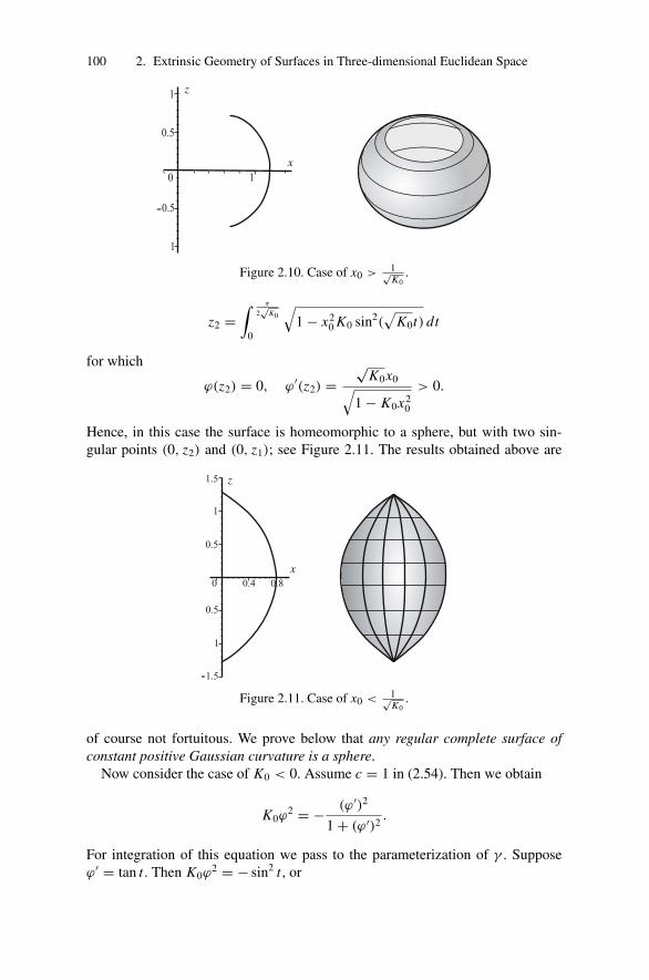
100 2. Extrinsic Geometry of Surfaces in Three-dimensional Euclidean Space
Figure 2.10. Case of x0 > 1√K0
.
z2 =∫ π
2√
K0
0
√1 − x2
0 K0 sin2(√
K0t) dt
for which
ϕ(z2) = 0, ϕ′(z2) =√
K0x0√1 − K0x2
0
> 0.
Hence, in this case the surface is homeomorphic to a sphere, but with two sin-gular points (0, z2) and (0, z1); see Figure 2.11. The results obtained above are
Figure 2.11. Case of x0 < 1√K0
.
of course not fortuitous. We prove below that any regular complete surface ofconstant positive Gaussian curvature is a sphere.
Now consider the case of K0 < 0. Assume c = 1 in (2.54). Then we obtain
K0ϕ2 = − (ϕ′)2
1 + (ϕ′)2.
For integration of this equation we pass to the parameterization of γ . Supposeϕ′ = tan t . Then K0ϕ
2 = − sin2 t , or
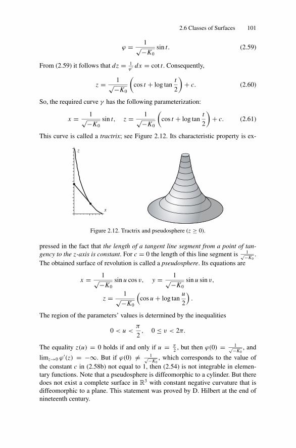
2.6 Classes of Surfaces 101
ϕ = 1√−K0sin t. (2.59)
From (2.59) it follows that dz = 1ϕ′ dx = cot t . Consequently,
z = 1√−K0
(cos t + log tan
t
2
)+ c. (2.60)
So, the required curve γ has the following parameterization:
x = 1√−K0sin t, z = 1√−K0
(cos t + log tan
t
2
)+ c. (2.61)
This curve is called a tractrix; see Figure 2.12. Its characteristic property is ex-
Figure 2.12. Tractrix and pseudosphere (z ≥ 0).
pressed in the fact that the length of a tangent line segment from a point of tan-gency to the z-axis is constant. For c = 0 the length of this line segment is 1√−K0
.The obtained surface of revolution is called a pseudosphere. Its equations are
x = 1√−K0sin u cos v, y = 1√−K0
sin u sin v,
z = 1√−K0
(cos u + log tan
u
2
).
The region of the parameters’ values is determined by the inequalities
0 < u <π
2, 0 ≤ v < 2π.
The equality z(u) = 0 holds if and only if u = π2 , but then ϕ(0) = 1√−K0
, and
limz→0 ϕ′(z) = −∞. But if ϕ(0) �= 1√−K0, which corresponds to the value of
the constant c in (2.58b) not equal to 1, then (2.54) is not integrable in elemen-tary functions. Note that a pseudosphere is diffeomorphic to a cylinder. But theredoes not exist a complete surface in R3 with constant negative curvature that isdiffeomorphic to a plane. This statement was proved by D. Hilbert at the end ofnineteenth century.
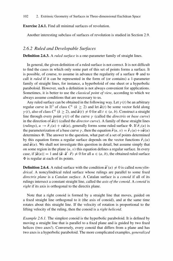
102 2. Extrinsic Geometry of Surfaces in Three-dimensional Euclidean Space
Exercise 2.6.1. Find all minimal surfaces of revolution.
Another interesting subclass of surfaces of revolution is studied in Section 2.9.
2.6.2 Ruled and Developable Surfaces
Definition 2.6.3. A ruled surface is a one-parameter family of straight lines.
In general, the given definition of a ruled surface is not correct. It is not difficultto find the cases in which only some part of this set of points forms a surface. Itis possible, of course, to assume in advance the regularity of a surface � and tocall it ruled if it can be represented in the form of (or contains) a 1-parameterfamily of straight lines, for instance, a hyperboloid of one sheet or a hyperbolicparaboloid. However, such a definition is not always convenient for applications.Sometimes, it is better to use the classical point of view, according to which wealways assume conditions that are necessary to us.
Any ruled surface can be obtained in the following way. Let γ (t) be an arbitraryregular curve in R3 of class Ck (k ≥ 2) and let �a(t) be some vector field alongγ (t), also of class Ck (k ≥ 2), and �a(t) �= 0 for all t ∈ (a, b). Construct a straightline through every point γ (t) of the curve γ (called the directrix or base curve)in the direction of �a(t) (called the director curve). A family of these straight lines(rulings), u → �r1(u) + v�a(u), generally forms some ruled surface �. If �r1(u) isthe parameterization of a base curve γ , then the equation �r(u, v) = �r1(u)+v�a(u)
determines �. The answer to the question, what part of a set of points determinedby this equation forms a regular surface depends on the vector functions �r1(u)
and �a(u). We shall not investigate this question in detail, but assume simply thaton some region in the plane (u, v) this equation defines a regular surface. In everycase, if |�a(u)| = 1 and (�a · �a′ · �r) �= 0 for all u ∈ (a, b), the obtained ruled surface� is regular at each of its points.
Definition 2.6.4. A ruled surface with the condition �a′(u) �= 0 is called noncylin-
drical. A noncylindrical ruled surface whose rulings are parallel to some fixeddirectrix plane is a Catalan surface. A Catalan surface is a conoid if all of itsrulings intersect a constant straight line, called the axis of the conoid. A conoid isright if its axis is orthogonal to the directix plane.
Note that a right conoid is formed by a straight line that moves, guided ona fixed straight line orthogonal to it (the axis of conoid), and at the same timerotates about this straight line. If the velocity of rotation is proportional to thelifting velocity of the ruling, then the conoid is a right helicoid.
Example 2.6.1. The simplest conoid is the hyperbolic paraboloid. It is defined bymoving a straight line that is parallel to a fixed plane and is guided by two fixedhelices (two axes!). Conversely, every conoid that differs from a plane and hastwo axes is a hyperbolic paraboloid. The more complicated examples, generalized

2.6 Classes of Surfaces 103
Plucker’s conoids (having n ≥ 2 folds; see Figure 2.136 with n = 2, 5) areobtained by rotation of a ray about the axis O Z and with simultaneous oscillatorymotion (with period 2πn) along the segment [−1, 1] of the axis:
�r = [0, 0, sin(nu)] + v[cos u, sin u, 0] = [v cos u, v sin u, sin(nu)].
(a) n = 2. (b) n = 5.
Figure 2.13. Generalized Plucker’s conoids.
We now find an expression for the Gaussian curvature of a ruled surface
�ru = �r1′ + �a′
v, �rv = �a, �ruu = �r1′′ + �a′′
v, �ruv = �a′, �rvv = 0.
From the last equality it follows that the coefficient N of the second fundamentalform is zero. Thus the Gaussian curvature of � is expressed by the formula
K = − M2
EG − F2. (2.62)
Formula (2.62) shows us that the Gaussian curvature of any ruled surface is non-positive, which of course does not surprise us, because at each point P ∈ � in thedirection of the vector �a the normal curvature is zero, and consequently, either theprincipal curvatures are of opposite signs or at least one of them is zero.
Consider in detail the case that the Gaussian curvature of a ruled surface isidentically zero. We calculate the coefficient M to be
M = (�ru · �rv · �ruv)√EG − F2
= ((�r1′ + v�a′
) · �a · �a′)√
EG − F2,
and consequently, the equality K = 0 means that
(�r1′(u) · �a(u) · �a′
(u)) = 0. (2.63)
Equality (2.63) holds in the following obvious cases:
6 For other examples of ruled surface modeling with Maple, see Figures 2.2, 2.14 and [Rov1].

104 2. Extrinsic Geometry of Surfaces in Three-dimensional Euclidean Space
1. �r1′(u) ≡ 0. Hence the base curve γ is a point, and � is a cone (without the
vertex).2. �a′
(u) ≡ 0. Hence �a(u) = const and � is a cylinder.3. �r1
′(u) × �a(u) = 0. A surface � is generated by lines tangent to the basecurve γ .
Example 2.6.2. Consider a four-leafed rose curve γ1 : ρ = cos(2ϕ), or in Carte-sian coordinates of the z = 1 plane, �r1(u) = [cos(2u) sin(u), cos(2u) cos(u), 1].Then the cylinder with base curve γ = γ1 and the z-axis is given by �r(u, v) =�r1(u) + v[0, 0, 1] = [cos(2u) cos(u), cos(2u) sin(u), 1]. The cone with directorcurve �a = γ1 and vertex S(0, 0, 0) is given by �r(u, v) = v�r1(u). These surfaces,drawn with Maple, are shown in Figure 2.14.
(a) Cylinder. (b) Cone.
Figure 2.14. Cylinder and cone over a four-leafed rose.
Consider now the general case. From equality (2.63) it follows that
�r1′(u) = λ1(u)�a(u) + λ2(u)�a′
(u),
where λ1 and λ2 are some functions of the variable u. Note further that since�r1
′(u) × �a′(u) �= 0, the function λ2(u) is nonzero and
�a × �a′ �= 0. (2.64)
Take the curve γ on a surface � defined by the equation v = v(u) or �r2(u) =�r1(u) + v(u)�a(u). We can select the function v(u) such that �r2
′(u) × �a ≡ 0. Weobtain the equation for function v = v(u),
(�r1′(u) + v′(u)�a(u) + v(u)�a′
(u)) × �a(u) = 0,
or(λ1(u)�a(u) + λ2(u)�a′
(u) + v′(u)�a(u) + v(u)�a′(u)) × �a(u) = 0,
or(λ2(u) + v(u)) · (�a′
(u) × �a(u)) = 0
2.6 Classes of Surfaces 105
and from (2.64) it follows that v(u) = −λ2(u). So for the curve γ and the vectorfield �a(u) we obtain case 3. Consequently, for any ruled surface � with zeroGaussian curvature that is not a cone or a cylinder, there is a curve such that� is generated by the family of tangent lines to this curve. Surfaces with zeroGaussian curvature are called developable. In the next section we shall prove thatany developable surface is ruled.
We now study the behavior of a tangent plane along generators of a developablesurface �. Let �n = �n(u, v) be a normal to �. Since the Gaussian curvature K iszero, a generator at each of its points goes along the main direction. Consequently,by Rodrigues’s theorem,
∂ �n∂v
= 0. (2.65)
Equation (2.65) shows us that in fact the normal �n(u, v) depends on u only; conse-quently, all tangent planes along a generator are parallel, and since they all containthe same straight line, they all coincide. This property of tangent planes along agenerator is called the stationarity of a tangent plane.
Finally, we study in detail the structure of a developable surface in a neigh-borhood of a base curve γ : �r = �r2(u). Divide � onto two semisurfaces �1 and�2 by the inequalities v ≥ 0 for �1 and v ≤ 0 for �2. We now calculate thecoefficients of the first fundamental form of the surface,
�ru = (�r2)u + v�a′(u), �rv = �a(u). (2.66)
If we assume u to be an arc length parameter of γ , and �a(u) = �r2′(u) a vector
field, then from (2.66) it follows that
E = 1 + k2v2, F = G = 1, (2.67)
where k(u) is the curvature of γ . From (2.67) one can see that at the points(u, v) ∈ �1 and (u, −v) ∈ �2, the coefficients E , F , and G coincide. Conse-quently, the semisurfaces �1 and �2 are isometric. Thus � is the union of twoisometric semisurfaces �1 and �2 that are “glued” to each other along the basecurve. Thus, we see that the surface � is not regular at the points of the base curveγ . At its other points, � is regular if the curvature k(u) of γ is nonzero at eachpoint, because |�ru × �rv|2 = EG − F2 = k2v2.
The semisurfaces �1 and �2 often intersect with each other. Here is the sim-plest example: Let γ be a circle in R2, and suppose the field �a(t) is a tangentvector field to γ . Then �1 and �2 obviously coincide, and � consists of twocopies of the exterior of a circle, “glued” along a circle.
We now explain why a ruled surface � with zero Gaussian curvature is calleda developable surface. Let P0(u0, v0) be a regular point of �. Take on � a neigh-borhood U of P0 defined by the inequalities |u − u0| < ε, |v − v0| < ε. Let ε besufficiently small such that the curvature k(u) of the base curve differs from zeroif |u − u0| < ε, and v �= 0 if |v − v0| < ε. Take a curve γ : �r = �ρ(u) on some

106 2. Extrinsic Geometry of Surfaces in Three-dimensional Euclidean Space
plane α such that its curvature k(u) coincides with k(u) for |u − u0| < ε and �a(u)
is the unit vector field tangent to γ . Then the region U of a plane α determined bythe condition �r = �ρ(u) + v�a(u) for u, v ∈ U is isometric to the region U on �,as is seen from (2.67). So, we can say that a neighborhood U of P0 is developed(unrolled) onto a plane.
Finally, note that if a complete regular surface � is developable, then � is acylinder (in particular, a plane).
2.6.3 Convex Surfaces
Recall that a region D ⊂ R3 is convex if together with each pair of its points Pand Q it contains the line segment P Q connecting these points. The boundary∂ D of a convex region D is actually a surface (generally, a continuous surface),and it is called a convex surface.
Theorem 2.6.1. If a convex region D contains a straight line, then the surface� = ∂ D is homeomorphic to a cylinder; if D contains a ray but does not containany straight line, then � = ∂ D is homeomorphic to a plane; if D does not containany ray (D is compact), then the surface � = ∂ D is homeomorphic to a sphere.
Proof. The statements of Theorem 2.6.1 are straightforward, and we shall proveonly the first of them. Let a be a straight line that lies entirely in D, and let Pbe an arbitrary point on �. Take two points P1 and P2 on the straight line a. Inview of the convexity of D, the line segments P P1 and P P2 belong to D. Letpoints P1 and P2 tend to infinity along the straight line a, and let the length ofthe line segment P1 P2 also tend to infinity. Then the line segments P P1 and P P2
tend to some rays a1 and a2 lying on the straight line a(P) that is parallel toa. Consequently, through each point P ∈ � there passes a straight line a(P)
that is parallel to a and lies entirely on �. Bring the plane α through some pointQ ∈ � and orthogonally to a. Since α ∩ D is a convex region on the plane α, theintersection α ∩ � is a convex curve γ . Let C be a cylinder whose directrix curveis γ and whose rulings are parallel to the straight line a. Since C is contained in� and is an open and closed set, they coincide, which completes the proof. �
The following obvious properties of convex surfaces are formulated as exer-cises.
Exercise 2.6.2. A regular surface � of class Ck (k ≥ 1) is convex if and only if itlies entirely on one side of every one of its tangent planes.
Exercise 2.6.3. The Gaussian curvature of a regular convex surface of class Ck
(k ≥ 2) is nonnegative at every point.
Exercise 2.6.4. The integral curvature (see Section 2.5) of a closed regular convexsurface of class C2 is 4π .
Hint. Use Gauss’s Theorem 2.5.2 (about spherical images).

2.6 Classes of Surfaces 107
Exercise 2.6.5. The exact upper bound of the integral curvature of any open, reg-ular, convex surface of class C2 is not greater than 2π .
Hint. Use Gauss’s Theorem 2.5.2 (about spherical images).
Exercise 2.6.6. The exact lower bound of the Gaussian curvature K (P) of anopen, regular, convex surface of class C2 is zero.
Hint. Use the statement of the previous exercise.
Exercise 2.6.7. If the Gaussian curvature K (P) of a regular convex surface ofclass C2 is not smaller than a positive real number a, then the surface is closed(compact).
Exercise 2.6.8. If a convex surface � is neither a cylinder nor a plane, then thereis a nondegenerate right circular cone containing �.
2.6.4 Problems: Curvature of Convex Surfaces
Now we formulate some conditions under which a regular surface of class C2 haspoints of positive Gaussian curvature.
Problem 2.6.2. On each closed (compact) regular surface � of class C2 there isa point at which the Gaussian curvature is positive.
Solution. Let S(O, R) be a sphere with center at some point O and radius R solarge that the entire surface � lies in this sphere. Decrease the radius of this sphereuntil the sphere and � touch each other for the first time, at which time the radiusof the sphere will be R1 < R. Denote by P a point that belongs to � ∩ S(O, R1).The tangent plane T �P at P is also a tangent plane to the sphere S(O, R1). Directa normal �n(P) inside of S(O, R1). The normal curvatures of S(O, R1) at thispoint are equal to 1/R1, and the normal curvatures of � are not smaller than 1/R1,because � lies entirely inside the sphere S(O, R1). Consequently, the Gaussiancurvature K (P) of � at P is not smaller than 1/(R1)
2. �
An analogous criterion for complete, noncompact (open) surfaces can be for-mulated as follows:
Problem 2.6.3. If an open, regular surface � of class C2 lies entirely inside aconvex circular cone T , then there is a point on � at which the Gaussian curvatureis positive.
Solution. Write down the equation of the cone T in the form x2 + y2 − a2z2 = 0,and define a region containing the surface � by the inequalities
x2 + y2 − a2z2 < 0, z > 0.
Take another cone T1, defined by the equation
108 2. Extrinsic Geometry of Surfaces in Three-dimensional Euclidean Space
x2 + y2 − b2(z + c)2 = 0 (where b > a, c > 0). (2.68)
Let H be one (upper) sheet of the hyperboloid of revolution of two sheets givenby the equation
4b2
c2(x2 + y2) − 4
c2(z + c)2 = −1, z ≥ − c
2.
This convex surface H lies entirely between the cones T and T1, and the cone T1
is asymptotic to H . Letρ0 = inf
P∈D,Q∈H|P Q|.
From the condition b > a in (2.68), follows that ρ0 exists and is finite, and thatthere exist points P0 and Q0 on the surfaces � and H such that ρ0 = |P0 Q0|.Now displace H parallel to itself by the vector
−−→P0 Q0. Denote by H0 the result-
ing surface. The surfaces H0 and � have a common tangent plane at P0, and �
lies entirely inside the convex region bounded by H0. Thus, as in the previousproblem, the Gaussian curvature of the surface � at P0 is not smaller than theGaussian curvature of the surface H0 at Q0, which is positive. �
Remark 2.6.2. If a convex surface � has a point at which the Gaussian curvatureis positive, then there is a right circular cone T containing � (see Exercise 2.6.8).
Thus from Problem 2.6.3 we obtain the following corollary.
Corollary 2.6.1. If a complete, open regular surface � lies entirely inside a con-vex region bounded by a convex surface �1 whose Gaussian curvature is positiveat least at one point, then there is a point on � at which the Gaussian curvature ispositive.
We now solve Hadamard’s problem.
Problem 2.6.4 (Hadamard). If the Gaussian curvature at each point of a closedregular surface � of class C2 is positive, then � is convex.
Hadamard’s problem is a particular case of Problem 2.6.5 given below. We shallgive another solution of this problem, different from but no less illuminating thanthe solution of Problem 2.6.5.
Solution. The surface � bounds some three-dimensional region, which will bedenoted by D. Take a point P on �, and direct a normal �n(P) to � at this point Pinside of D, and continue this direction of the normal by continuity to each pointon �. Define the sign of the normal curvature at each point of � by the directionof the normal �n(P). In view of the statement of Problem 2.6.2, there is a pointQ on � at which under the above definition of the sign of a normal curvature allnormal curvatures are positive. By the conditions of our problem, the Gaussiancurvature at all points P ∈ � is positive. It follows that the normal curvatures of� are positive at all of its points. Now let Q be some point in int D. Denote by

2.6 Classes of Surfaces 109
�Q the set of points int D that can be connected with Q by a line segment entirelycontained in int D. Obviously, �Q is an open set in int D.
We prove that �Q is closed in int D. Let Q0 ∈ int D be a point such that there isa sequence of points Qn ∈ �Q tending to Q0. Assume that Q0 �∈ �Q . That meansthat the line segment Q Q0 touches � at some point P that lies inside of the linesegment Q Q0 (P ∈ Q Q0, P �= Q, P �= Q0). Then
−−→P Q0 belongs to the tangent
plane T �P , and the normal curvature of � at the point P and in the direction ofthe vector
−−→P Q0 is nonpositive, which is a contradiction. �
Problem 2.6.5. Let � be a closed, regular surface of class C2 immersed in R3.Then if the Gaussian curvature of the surface � at each of its points is nonnega-tive, then � is convex, and consequently, an embedded surface.
Solution. Assume the opposite and lead this assumption to a contradiction. If �
is a nonconvex surface, then there is a plane α such that the set α ∩ � is notconnected, because in the opposite case, � will lie on one side of each of itstangent planes and will be convex. Take a point Q on the plane α and a unit vector�e orthogonal to the plane α. Define a function fα(P) on �, assuming it to be equalto (
−→Q P, �e). Note that in view of Problem 2.5.1, we can assume that fα(P) has
no degenerate critical points on the surface �. Let P1 and P2 be two points in theset �∩α from its different connected components. Without loss of generality, wemay suppose that there is a continuous curve σ(t) (0 ≤ t ≤ 1) on � connectingP1 and P2 and belonging to the region defined by the inequality fα(P) ≥ 0. Let�(P1 P2) be the class of all continuous curves σ on � with endpoints P1 and P2
that lie in the region fα(P) ≥ 0. Take a point Pσ on each curve σ ∈ �(P1 P2) atwhich the function fα(σ (t)) for 0 ≤ t ≤ 1 reaches its maximum. Define a realnumber a0 by the equality
a0 = infσ∈�(P1 P2)
fα(Pσ ).
Obviously, a0 > 0. In view of the compactness of � and the definition of a0, thereis a point P0 on � such that fα(P0) = Q0; and there exist points Q1 �= P0 andQ2 �= P0 in any neighborhood of P0 on the surface � such that
fα(Q1) ≤ a0, (2.69)
fα(Q2) ≥ a0. (2.70)
In view of the definition of a0 and of the point P0, a plane T �P0 is parallel tothe plane α. Introduce a rectangular Cartesian coordinate system x , y, z with theorigin at P0; direct the axis O Z parallel to the vector �e, and so the axes O X andOY are located in the plane T �P0 . The equation of � in some neighborhood ofP0 can be written explicitly as
z = h(x, y).
The function h(x, y) satisfies the equations

110 2. Extrinsic Geometry of Surfaces in Three-dimensional Euclidean Space
h(0, 0) = 0,∂h
∂x(0, 0) = ∂h
∂y(0, 0) = 0;
moreover, the axes O X and OY can be chosen so that
∂2h
∂x∂y(0, 0) = 0.
We introduce the notation
a = 1
2
∂2h
∂x2(0, 0), b = 1
2
∂2h
∂y2(0, 0).
Write Taylor’s formula for the function h(x, y):
h(x, y) = ax2 + by2 + o(x2 + y2). (2.71)
Since the functions h(x, y) and fα(P) in a neighborhood of the point P0 arerelated by the equality fα(x, y) = h(x, y)+a0, and since fα(0) has no degeneratecritical points on �, P0 is a degenerate critical point of the function h(x, y). Thusa · b �= 0 holds. If we assume that a · b > 0, then in view of (2.71), this leadsto a contradiction either with the inequality (2.69) or with the inequality (2.70).Consequently, a · b < 0. But then the Gaussian curvature K of �, equal to 4a · b,would be negative, which contradicts the conditions of the problem. The problemis solved. �
Now we study open (i.e., complete noncompact) surfaces.
Problem 2.6.6. If the Gaussian curvature of an open regular surface � of classC2 is everywhere positive, then � is convex.
Hint. Repeat the considerations and constructions of Problem 2.6.4.
An analogue of Problem 2.6.5 appears to be more complicated. The followingstatement holds.
Problem 2.6.7. Let � be an open regular surface of class C2 immersed in R3.Then if the Gaussian curvature of � at each of its points is nonnegative and thereis a point of positive Gaussian curvature, then � is convex and consequently, anembedded surface.
The solution of this problem is difficult and long. It can be found in [Pog]. Wenow give some tests that allow us to estimate from above the principal curvaturesof a surface at some points of this surface.
Problem 2.6.8. If a region D bounded by a convex surface � of class C2 con-tains a ball C(R) of radius R, then there is a point P on � at which all normalcurvatures are not greater than 1/R.

2.6 Classes of Surfaces 111
Solution. Increase the radius of the ball C(R) while its center is fixed until it (theball C(R1), R1 > R) touches the surface � for the first time at some point P0. Sowe have obtained that � touches the ball C(R1) at P0 and lies outside of the ballC(R1). From this it follows that the absolute value of any normal curvature is notgreater than 1/R1, and consequently, than 1/R. �Remark 2.6.3. The convexity assumption for the surface � is not essential whenthe sign of the normal curvature of � is defined by the direction of its inner nor-mal.
This test is essentially strengthened in the following problem.
Problem 2.6.9. Let � be a convex, regular surface of class C2 bounded by a con-vex region D. Then, if one can place a circle with radius R entirely inside ofD, there is a point on � at which all the normal curvatures are not greater than1/R. (The sign of the normal curvature is determined by the direction of the innernormals.)
Solution. Let K R be a disk of radius R that lies entirely in D, and let α be theplane containing this disk. Denote by C the right circular cylinder whose gener-atrix is the boundary of the disk K R , and the rulings are straight lines orthogonalto the plane α. The following two cases are possible:
(1) the cylinder C does not intersect the surface �,
(2) the cylinder C cuts out from the surface � at least one surface �1.
In the first case, as follows from Theorem 2.6.1, � itself is a cylinder C , andthe statement of the problem becomes obvious.
Consider the second case. Let D be the region bounded by the cylinder C and�1. Let S(R − ε) be the sphere of radius R − ε (0 < ε < R) with center on theaxis of the cylinder C that does not intersect �1. Move the sphere S(R − ε) in thedirection toward �1 until the first tangency of S(R − ε) and �1 appears, and letP be a point of tangency. The surface �1, as follows from our construction, liesentirely on one side of S(R − ε) and touches it at P , an interior point of �1. Thusall normal curvatures of �1 at P are not greater than 1
R−ε. Since ε may be chosen
as close to zero as possible, the statement of the problem is proved. �There are many books and surveys devoted to convex surfaces and bodies with-
out any smoothness assumptions; see [Ku1], [Bus], [Sto], [Pog], [Hop].
2.6.5 Saddle Surfaces
Definition 2.6.5. A regular surface � of class C2 is called a saddle surface if theGaussian curvature at each point of � is nonpositive.
Note that the class of saddle surfaces contains the well-studied class of minimalsurfaces, i.e., surfaces whose mean curvature H is identically zero,7
7 See, for example, [OG].

112 2. Extrinsic Geometry of Surfaces in Three-dimensional Euclidean Space
Generally speaking, there is another definition of a saddle surface that is alsoapplicable for a continuous surface and coincides with our definition in the regularcase.
If the Gaussian curvature of � is negative at some point P ∈ �, then thetangent plane T �P intersects �, and the surface lies on both sides of T �P . Thesurface � has a saddle-type shape in a neighborhood of such a point, which is thereason for the name of these surfaces. One of the features of a complete saddlesurface is its unboundness in R3. So for instance, from Problem 2.6.2 it followsthat there does not exist a closed saddle surface in R3, and from Problem 2.6.3 (orits Corollary 2.6.1) it follows that one cannot place a saddle surface entirely inany strictly convex region. But a saddle surface can be entirely placed between twoparallel planes, for instance, a circular cylinder or, a more interesting example, thesurface obtained by rotation of the curve x = z2
1−z2 (|z| < 1) about the axis O Z .The Gaussian curvature of this surface is negative at each point. But this procedureis impossible for saddle surfaces homeomorphic to a plane.
Theorem 2.6.2 (S.N. Bernstein). If a saddle surface � defined by the equation
z = f (x, y) (−∞ < x, y < ∞)
has points of negative Gaussian curvature, then
supx,y
| f (x, y)| = ∞.
The proof of this theorem is very difficult and cannot be given here. We nowstudy the behavior of the Gaussian curvature K (P) and the principal curvaturesk1(P) and k2(P) of saddle surfaces.
The strongest result concerning the behavior of the Gaussian curvature on asaddle surface was obtained by N.V. Efimov.
Theorem 2.6.3 (N.V. Efimov ). The least upper bound of the Gaussian curvatureon a complete saddle surface in R3 is zero.
This theorem of N.V. Efimov is very deep and difficult to prove. It is an essentialgeneralization of the well-known theorem of Hilbert on the nonexistence in R3 ofa complete regular surface with constant negative Gaussian curvature. In thisbook we cannot give its proof. We restrict ourselves to only the proof of Hilbert’stheorem given at the end of Section 2.8.
The statements of N.V. Efimov’s theorem and Exercise 2.6.6 can be formulatedin the form of a single theorem.
Theorem 2.6.4. The exact lower bound of the absolute value of the Gaussian cur-vature of a complete open regular surface in R3 is zero.
Let us now study the behavior of the principal curvatures k1(P) and k2(P) atinfinity for any complete saddle surface.
2.6 Classes of Surfaces 113
Problem 2.6.10. Prove that if on a complete saddle surface � ⊂ R3,
infP∈�
|k1(P)| + infP∈�
|k2(P)| = c > 0
holds, then � is a cylinder, i.e., k1(P) ≡ 0 and k2(P) = const.
Solution. Assume for definiteness that k1(P) ≤ 0 and k2(P) ≥ 0 and thatinfP∈� |k2(P)| = c1 > 0. Assume that the Gaussian curvature K (P) is not iden-tically zero, and show that this leads to a contradiction. Take a real number R,satisfying the inequality
R >1
c1. (2.72)
Then the Gaussian curvature of a parallel surface �(R) is nonnegative. Indeed,by Theorem 2.4.6 we have
k1(P, R) = k1(P)
1 − Rk1(P), k2(P, R) = k2(P)
1 − Rk2(P).
From this, we obtain
K (P, R) = K (P)
(1 − Rk1(P))(1 − Rk2(P)).
The numerator and denominator of this fraction are negative. Indeed, K (P) ≤ 0by the conditions of the problem, 1 − Rk1(P) > 0 because of k1(P) ≤ 0, and1 − Rk2(P) < 0 in view of inequality (2.72). From the nonnegativity of theGaussian curvature of �(R), it follows (see Exercise 2.6.8) that �(R) can beplaced entirely inside of a strictly convex cone C . Take another strongly convexcone C1 such that it contains C and the distance from any point of C to C1 isgreater than R. Then a saddle surface � lies entirely in the cone C , which isimpossible (see Problem 2.6.3). Thus, the Gaussian curvature of � is identicallyzero. �
In 1966, J. Milnor enunciated a conjecture, which for saddle surfaces impliesthat for statement 2.6.10 to hold, it suffices that:
infP∈�
(|k1(P)| + |k2(P)|) �= 0.
This assertion is not yet been proved.We solve one more problem, in which saddle and convex surfaces are closely
related.
Problem 2.6.11. Let � be a regular convex surface of class Ck (k ≥ 2), and k1(P)
and k2(P) the principal curvatures of � at a point P . Suppose that 0 ≤ k1(P) ≤k2(P). In this case, if supP∈� k1(P) < infP∈� k2(P), then � is a cylinder, andconsequently, k1 ≡ 0, but k2 = c0 > 0. The sign of the normal curvature isdetermined by the direction of the inner normal.

114 2. Extrinsic Geometry of Surfaces in Three-dimensional Euclidean Space
Solution. We assume that � is not a cylinder, and show this leads to a contradic-tion. The surface � cannot be homeomorphic to a sphere, because on any suchsurface there is an umbilic at which k1(P) = k2(P), in contradiction to the con-dition of the problem. Thus we need only study the case that � is homeomorphicto a plane; in this case we may suppose that supP∈� k1(P) = c1 > 0. Definec2 = infP∈� k2(P), and denote by R a real number satisfying the inequality
1
c2< R <
1
c1. (2.73)
Take parallel surfaces �(R) and �(−R). The surface �(−R) is convex and con-tains �(R) entirely. Prove that �(R) is regular and a saddle surface. The regular-ity of �(R) follows from Theorem 2.4.6. We now calculate the principal curva-tures of �(R) at a point ϕ(P). (We use the notation introduced in Section 2.4.9).By Theorem 2.4.6,
k1(P, R) = k1(P)
1 − Rk1(P), k2(P, R) = k2(P)
1 − Rk2(P).
Thus the Gaussian curvature K (P, R) of �(R) is expressed by the formula
K (P, R) = K (P)
(1 − Rk1(P))(1 − Rk2(P)). (2.74)
The numerator of this fraction is nonnegative, and the denominator is negative. Infact, in view of (2.73),
1 − Rk1(P) ≥ 1 − c1 R > 0, (2.75)
but
1 − Rk2(P) ≤ 1 − c2 R < 0. (2.76)
Thus, from (2.74) – (2.76) follows that
K (P, R) ≤ 0.
So a saddle surface �(R) lies entirely inside of the convex surface �(−R), whichis impossible. �
2.7 Some Classes of Curves on a Surface
2.7.1 Lines of Curvature
Definition 2.7.1. A smooth curve γ on a regular surface � of class C2 is called aline of curvature if the tangent vector of γ is a principal vector of � at all pointsof γ .
2.7 Some Classes of Curves on a Surface 115
Recall the equation determining the principal vectors∣∣∣∣∣∣−(λ2)2 λ1λ2 −(λ1)2
E F GL M N
∣∣∣∣∣∣ = 0.
If u = u(t), v = v(t) are equations of some curve, then its tangent vector has ina local base the coordinates u′(t) and v′(t). Thus the problem of existence of thelines of curvature is reduced to the problem of the existence of a solution to thefollowing differential equation:
(L F − E M)(u′)2 − (E N − LG)u′v′ + (MG − N F)
(v′)2 = 0.
From Lemma 2.1.1 it follows that through each nonumbilical point of the surface� it is possible to pass a line of curvature and then to extend it until we reach anumbilic.
From the same lemma it follows that in a neighborhood of any nonumbilicalpoint one can construct a coordinate system such that the lines of curvature willbecome the coordinate curves. The characteristic indication of such a coordinatesystem is the fulfilment of the following equalities: M = F = 0. In fact, ifthe coordinate curves are the lines of curvature, then F = 0 in view of theirorthogonality, and M = 0, since the principal vectors are conjugate with respectto the second fundamental form.
We now consider some geometric properties of the lines of curvature.
Theorem 2.7.1. A ruled surface C formed by the family of normal straight linesto � along the lines of curvature has nonzero Gaussian curvature.
Proof. Let �r = �r(t) be the equation of a line of curvature γ , and �n(t) the di-rections of the normals to � along γ . Then the equation of the surface C can bewritten in the form
�r = �r(u, v) = �r(u) + v�n(u).
By Rodrigues’s theorem, �n′(u) = −k�r ′
(u), and consequently, see (2.64), theGaussian curvature of the surface � is zero. �
Theorem 2.7.2. If two surfaces �1 and �2 intersect with a constant angle andthe curve of intersection is a line of curvature on one of them, then it is also a lineof curvature on the other surface.
Proof. Let �r = �r(t) be the equation of the curve of intersection of the surfaces �1
and �2. Denote by �n1 and �n2 the unit normals to �1 and �2 along γ , respectively.From the conditions of the theorem we obtain the equations
〈�n1(t), �n2(t)〉 = const, (2.77)
d �n1
dt= −k(t)�r ′
(t), (2.78)
〈�r ′(t), �n1〉 = 〈�r ′
(t), �n2〉 = 0. (2.79)
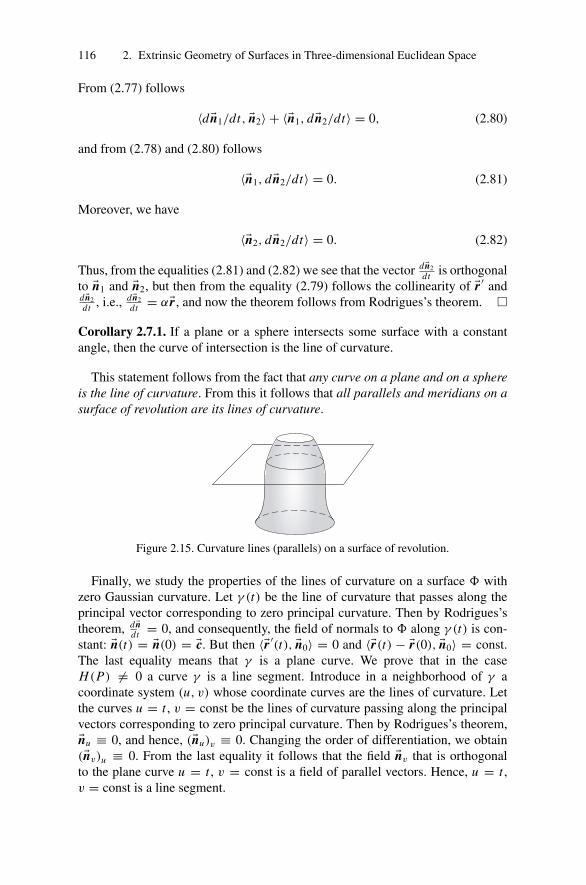
116 2. Extrinsic Geometry of Surfaces in Three-dimensional Euclidean Space
From (2.77) follows
〈d �n1/dt, �n2〉 + 〈�n1, d �n2/dt〉 = 0, (2.80)
and from (2.78) and (2.80) follows
〈�n1, d �n2/dt〉 = 0. (2.81)
Moreover, we have
〈�n2, d �n2/dt〉 = 0. (2.82)
Thus, from the equalities (2.81) and (2.82) we see that the vector d �n2dt is orthogonal
to �n1 and �n2, but then from the equality (2.79) follows the collinearity of �r ′ andd �n2dt , i.e., d �n2
dt = α�r , and now the theorem follows from Rodrigues’s theorem. �
Corollary 2.7.1. If a plane or a sphere intersects some surface with a constantangle, then the curve of intersection is the line of curvature.
This statement follows from the fact that any curve on a plane and on a sphereis the line of curvature. From this it follows that all parallels and meridians on asurface of revolution are its lines of curvature.
Figure 2.15. Curvature lines (parallels) on a surface of revolution.
Finally, we study the properties of the lines of curvature on a surface � withzero Gaussian curvature. Let γ (t) be the line of curvature that passes along theprincipal vector corresponding to zero principal curvature. Then by Rodrigues’stheorem, d �n
dt = 0, and consequently, the field of normals to � along γ (t) is con-stant: �n(t) = �n(0) = �c. But then 〈�r ′
(t), �n0〉 = 0 and 〈�r(t) − �r(0), �n0〉 = const.The last equality means that γ is a plane curve. We prove that in the caseH(P) �= 0 a curve γ is a line segment. Introduce in a neighborhood of γ acoordinate system (u, v) whose coordinate curves are the lines of curvature. Letthe curves u = t , v = const be the lines of curvature passing along the principalvectors corresponding to zero principal curvature. Then by Rodrigues’s theorem,�nu ≡ 0, and hence, (�nu)v ≡ 0. Changing the order of differentiation, we obtain(�nv)u ≡ 0. From the last equality it follows that the field �nv that is orthogonalto the plane curve u = t , v = const is a field of parallel vectors. Hence, u = t ,v = const is a line segment.

2.7 Some Classes of Curves on a Surface 117
Theorem 2.7.3. A regular surface � of class Ck (k ≥ 2) with zero Gaussiancurvature is a ruled surface, and hence is either a cone or a cylinder, or it isformed by the family of tangent lines to some space curve.
If the surface has nonzero mean curvature, then the statement of Theorem 2.7.3is proved, because in this case the second principal curvature differs from zero. Inthe general case, the proof of Theorem 2.7.3 requires a more delicate approach,which we omit.
2.7.2 Asymptotic Curves
Definition 2.7.2. A tangent vector �λ ∈ T �P at a point P is called an asymptoticdirection if I I (�λ) = 0; i.e., the normal curvature of a surface � in this directionis zero.
Definition 2.7.3. An asymptotic curve is a smooth curve γ on a surface � whosetangent vector is an asymptotic direction at each point.
From Euler’s formula one can see that asymptotic directions exist only at hy-perbolic or parabolic points on a regular surface �. Moreover, at hyperbolic pointsthere are two such directions, and at parabolic points, there is one.
Equations of asymptotic curves result directly from their definition. If u = u(t),v = v(t) are parametric equations of an asymptotic curve, then the functions u(t)and v(t) must satisfy the differential equation
L (du/dt)2 + 2M(du/dt) · (dv/dt) + N (dv/dt)2 = 0. (2.83)
From Lemma 2.1.1 it immediately follows that in a neighborhood of a hyperbolicpoint there is a coordinate system in which the coordinate curves are the asymp-totic curves.
From (2.83) it follows that coordinate curves are asymptotic curves if and onlyif L = N = 0. Indeed, if u = t , v = const is an asymptotic curve, then L · 1 +2M · 0 + N · 0 = 0 or L = 0, analogously, if u = const, v = t is an asymptoticcurve, then N = 0. Conversely, if L = N = 0, then (2.83) takes the form
M(du/dt) · (dv/dt) = 0. (2.84)
If M �= 0, then (2.84) has two solutions: u = f (t), v = const and u = const,v = f (t); i.e., the coordinate curves are the asymptotic curves. If M = 0, then asurface � in a neighborhood of the point under discussion is a plane, and each ofits curves is an asymptotic curve.
We now study the geometrical characteristic of asymptotic curves.
Theorem 2.7.4. If γ is an asymptotic curve on a regular surface � of class Ck
(k ≥ 3), then a tangent plane to � is an osculating plane of a curve γ at eachpoint γ (t).

118 2. Extrinsic Geometry of Surfaces in Three-dimensional Euclidean Space
Proof. Consider an arbitrary point γ (t) on the curve γ . Since the normal cur-vature of � in the direction of the tangent vector �τ = γ (t) is zero, then byMeusnier’s theorem, either the curvature of γ is zero at this point, or the anglebetween the principal normal �ν(t) to γ and the normal �n(t) to � at the point γ (t)is π
2 . In the first case, any plane containing �τ (t) is an osculating plane, includingT �P , and in the second case, the plane T �P contains both �τ (t) and �ν(t), andhence it is again osculating.
Consider in detail a vector field �n(t) along the asymptotic curve γ (t). For thosepoints where the torsion of γ (t) exists, the vector �n(t) equals ±�β(t), and henceκ2 = ∣∣ d �n
dt
∣∣2; and for those points where the curvature of γ is zero and the torsion
is not determined, we define it in addition, supposing that κ2 = ∣∣ d �ndt
∣∣2. Here t isthe arc length parameter of a curve. �
Keeping in mind this remark, we formulate the Beltrami–Enneper theorem.
Theorem 2.7.5. The square of the torsion of an asymptotic curve on a regularsurface of class Ck (k ≥ 3) at each of its points is equal to the Gaussian curvatureof the surface at this point, considered with the opposite sign.
Proof. By definition,κ2 = |d �n/dt |2 = I I I (�τ ),
where �τ is the tangent vector to the asymptotic curve. By (2.45) we have I I I (�τ ) =−K · I (�τ ) + 2H · I I (�τ ), but by the condition of the theorem, I I (�τ ) = 0, in viewof the choice of parameter t : I (�τ ) = 1. Thus, we obtain κ2 = ( d �n
dt )2 = I I I (�τ ) =
−K . The theorem is proved. �
It is interesting to consider the particular case of the Beltrami–Enneper theoremin which an asymptotic curve γ is a straight line. Draw along γ (t) on the surface� the unit vector field �λ(t) orthogonal to γ (t),
�λ(t) ∈ T �γ(t), 〈�λ(t), �τ (t)〉 = 0.
Here we again assume that t is an arc length parameter on γ . Write down theequalities ⟨
�λ(t),d
dt�λ⟩
= 0, (2.85a)
〈�λ(t), �τ (t)〉 = 0, (2.85b)
�λ(t) = ±�τ (t) × �n(t), (2.85c)
�n(t) = ±�τ (t) × �λ(t), (2.85d)
d �τdt
= 0. (2.85e)
From (2.85c–e) we have

2.7 Some Classes of Curves on a Surface 119
d
dt�λ = ±�τ × d �n
dt,
d �ndt
= ±�τ × d
dt�λ, (2.86)
and from this it follows that ⟨d �ndt
, �τ⟩
= 0. (2.87)
From (2.85e) and (2.86) we obtain∣∣∣∣ d
dt�λ∣∣∣∣ = |�τ | ·
∣∣∣∣d �ndt
∣∣∣∣ · sinπ
2=∣∣∣∣d �n
dt
∣∣∣∣ .Consequently, (
d
dt�λ)2
=(
d �ndt
)2
= κ2 = −K .
We have thus proved the following theorem.
Theorem 2.7.6. Let a regular surface � of class Ck (k ≥ 3) contain a straightline γ , and let �λ(t) be the field of unit vectors along the straight line γ (t) thatare tangent to � and orthogonal to γ . Then the Gaussian curvature K is equal to−| d
dt�λ|2, where t is the arc length of γ .
2.7.3 Geodesics on a Surface
Here we give the definition and study the simplest properties of the most beautifulclass of curves on a surface: the class of geodesics. We first define the notion ofgeodesic curvature of a curve on a surface �. Let γ (t) (a ≤ t ≤ b) be a regularcurve of class C2 on a regular surface � of class C2. Let t be the arc length of thecurve γ (t), counting from one of its points.
Denote, as usual, by k(t) the curvature of γ at the point γ (t), by �τ (t) and �ν(t)the tangent vector and principal normal vector at the point γ (t), and by ϕ(t) theangle between �ν(t) and �n(t). The geodesic curvature kg(t) of the curve γ at thepoint γ (t) is defined by the formula
kg(t) = k(t) · sin ϕ(t). (2.88)
In other words, the geodesic curvature kg(t) of γ at the point γ (t) is the normof the projection of the vector k(t)�ν(t) onto the tangent plane T �γ(t) to �. Recallfor comparison that the normal curvature of the curve γ (the normal curvature of� in the direction �τ ) is the projection of k(t)�ν(t) onto �n. Find the formula forcalculation of kg . From (2.88) and Theorem 1.6.1 it follows that
kg(t) = k(t) · sin ϕ(t) = k(t) · |〈�ν × �n, �τ 〉| = (k(t)�ν · �τ · �n) = (�r ′′ · �r ′ · �n).
It is not difficult to derive that if t is an arbitrary parameter, then
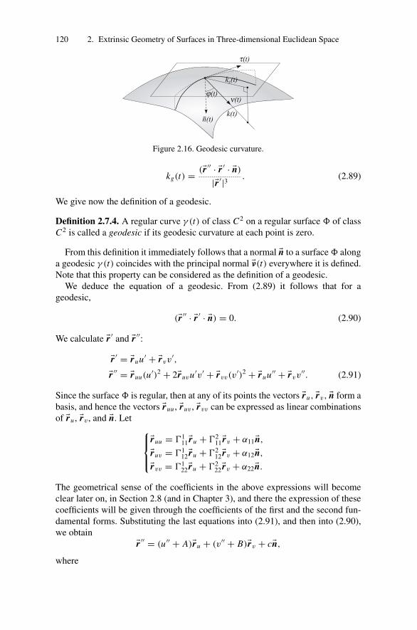
120 2. Extrinsic Geometry of Surfaces in Three-dimensional Euclidean Space
Figure 2.16. Geodesic curvature.
kg(t) = (�r ′′ · �r ′ · �n)
|�r ′|3 . (2.89)
We give now the definition of a geodesic.
Definition 2.7.4. A regular curve γ (t) of class C2 on a regular surface � of classC2 is called a geodesic if its geodesic curvature at each point is zero.
From this definition it immediately follows that a normal �n to a surface � alonga geodesic γ (t) coincides with the principal normal �ν(t) everywhere it is defined.Note that this property can be considered as the definition of a geodesic.
We deduce the equation of a geodesic. From (2.89) it follows that for ageodesic,
(�r ′′ · �r ′ · �n) = 0. (2.90)
We calculate �r ′ and �r ′′:
�r ′ = �ruu′ + �rvv′,
�r ′′ = �ruu(u′)2 + 2�ruvu′v′ + �rvv(v
′)2 + �ruu′′ + �rvv′′. (2.91)
Since the surface � is regular, then at any of its points the vectors �ru, �rv, �n form abasis, and hence the vectors �ruu , �ruv , �rvv can be expressed as linear combinationsof �ru , �rv , and �n. Let ⎧⎪⎨⎪⎩
�ruu = �111�ru + �2
11�rv + α11�n,
�ruv = �112�ru + �2
12�rv + α12�n,
�rvv = �122�ru + �2
22�rv + α22�n.
The geometrical sense of the coefficients in the above expressions will becomeclear later on, in Section 2.8 (and in Chapter 3), and there the expression of thesecoefficients will be given through the coefficients of the first and the second fun-damental forms. Substituting the last equations into (2.91), and then into (2.90),we obtain
�r ′′ = (u′′ + A)�ru + (v′′ + B)�rv + c�n,
where
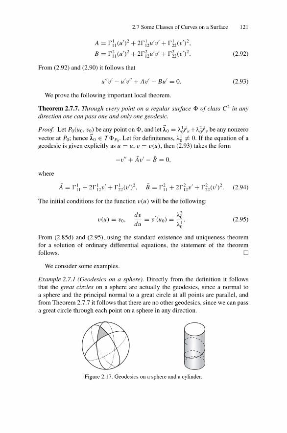
2.7 Some Classes of Curves on a Surface 121
A = �111(u
′)2 + 2�112u′v′ + �1
22(v′)2,
B = �211(u
′)2 + 2�212u′v′ + �2
22(v′)2. (2.92)
From (2.92) and (2.90) it follows that
u′′v′ − u′v′′ + Av′ − Bu′ = 0. (2.93)
We prove the following important local theorem.
Theorem 2.7.7. Through every point on a regular surface � of class C2 in anydirection one can pass one and only one geodesic.
Proof. Let P0(u0, v0) be any point on �, and let �λ0 = λ10�ru +λ2
0�rv be any nonzerovector at P0; hence �λ0 ∈ T �P0 . Let for definiteness, λ1
0 �= 0. If the equation of ageodesic is given explicitly as u = u, v = v(u), then (2.93) takes the form
−v′′ + Av′ − B = 0,
where
A = �111 + 2�1
12v′ + �1
22(v′)2, B = �2
11 + 2�212v
′ + �222(v
′)2. (2.94)
The initial conditions for the function v(u) will be the following:
v(u) = v0,dv
du= v′(u0) = λ2
0
λ10
. (2.95)
From (2.85d) and (2.95), using the standard existence and uniqueness theoremfor a solution of ordinary differential equations, the statement of the theoremfollows. �
We consider some examples.
Example 2.7.1 (Geodesics on a sphere). Directly from the definition it followsthat the great circles on a sphere are actually the geodesics, since a normal toa sphere and the principal normal to a great circle at all points are parallel, andfrom Theorem 2.7.7 it follows that there are no other geodesics, since we can passa great circle through each point on a sphere in any direction.
Figure 2.17. Geodesics on a sphere and a cylinder.
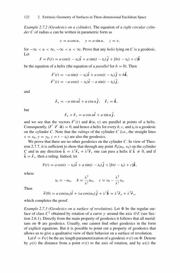
122 2. Extrinsic Geometry of Surfaces in Three-dimensional Euclidean Space
Example 2.7.2 (Geodesics on a cylinder). The equation of a right circular cylin-der C of radius a can be written in parametric form as
x = a cos u, y = a sin u, z = v,
for −∞ < u < ∞, −∞ < u < ∞. Prove that any helix lying on C is a geodesic.Let
�r = �r(t) = a cos(t − t0)�i + a sin(t − t0)�j + [b(t − t0) + c]�kbe the equation of a helix (the equation of a parallel for b = 0). Then
�r ′(t) = −a sin(t − t0)�i + a cos(t − t0)�j + b�k,
�r ′′(t) = −a cos(t − t0)�i − a sin(t − t0)�j ,
and
�ru = −a sin u�i + a cos u�j , �rv = �k,
but�ru × �rv = a cos u�i + a sin u�j ,
and we see that the vectors �r ′′(t) and �n(u, v) are parallel at points of a helix.
Consequently, (�r ′′ · �r ′ · �n) = 0, and hence a helix for every b, c, and t0 is a geodesicon the cylinder C . Note that the rulings of the cylinder C (i.e., the straight linesx = x0, y = y0, z = t − t0) are also the geodesics.
We prove that there are no other geodesics on the cylinder C . In view of Theo-rem 2.7.7, it is sufficient to show that through any point P0(u0, v0) on the cylinderC and in any direction �λ = λ1�ru + λ2�rv one can pass a helix if �λ �= 0, and if�λ = �rv , then a ruling. Indeed, let
�r(t) = a cos(t − t0)�i + a sin(t − t0)�j + [b(t − t0) + c]�k,
where
t0 = −u0, b = λ2
λ1u0, c = v0 − λ2
λ1v0.
Then�r(0) = a cos(u0)�i + λa cos(u0)�j + λ1�k = λ1�ru + λ2�rv,
which completes the proof.
Example 2.7.3 (Geodesics on a surface of revolution). Let � be the regular sur-face of class C2 obtained by rotation of a curve γ around the axis O Z (see Sec-tion 2.6.1). Directly from the main property of geodesics it follows that all merid-ians on � are geodesics. Usually, one cannot find other geodesics in the formof explicit equations. But it is possible to point out a property of geodesics thatallows us to give a qualitative view of their behavior on a surface of revolution.
Let �r = �r(t) be the arc length parameterization of a geodesic σ(t) on �. Denoteby ρ(t) the distance from a point σ(t) to the axis of rotation, and by α(t) the
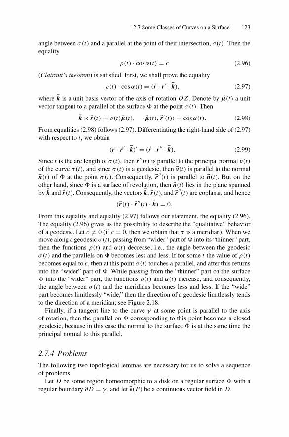
2.7 Some Classes of Curves on a Surface 123
angle between σ(t) and a parallel at the point of their intersection, σ(t). Then theequality
ρ(t) · cos α(t) = c (2.96)
(Clairaut’s theorem) is satisfied. First, we shall prove the equality
ρ(t) · cos α(t) = (�r · �r ′ · �k), (2.97)
where �k is a unit basis vector of the axis of rotation O Z . Denote by �µ(t) a unitvector tangent to a parallel of the surface � at the point σ(t). Then
�k × �r(t) = ρ(t)�µ(t), 〈�µ(t), �r ′(t)〉 = cos α(t). (2.98)
From equalities (2.98) follows (2.97). Differentiating the right-hand side of (2.97)with respect to t , we obtain
(�r · �r ′ · �k)′ = (�r · �r ′′ · �k). (2.99)
Since t is the arc length of σ(t), then �r ′′(t) is parallel to the principal normal �ν(t)
of the curve σ(t), and since σ(t) is a geodesic, then �ν(t) is parallel to the normal�n(t) of � at the point σ(t). Consequently, �r ′′
(t) is parallel to �n(t). But on theother hand, since � is a surface of revolution, then �n(t) lies in the plane spannedby �k and �r(t). Consequently, the vectors �k, �r(t), and �r ′′
(t) are coplanar, and hence
(�r(t) · �r ′′(t) · �k) = 0.
From this equality and equality (2.97) follows our statement, the equality (2.96).The equality (2.96) gives us the possibility to describe the “qualitative” behaviorof a geodesic. Let c �= 0 (if c = 0, then we obtain that σ is a meridian). When wemove along a geodesic σ(t), passing from “wider” part of � into its “thinner” part,then the functions ρ(t) and α(t) decrease; i.e., the angle between the geodesicσ(t) and the parallels on � becomes less and less. If for some t the value of ρ(t)becomes equal to c, then at this point σ(t) touches a parallel, and after this returnsinto the “wider” part of �. While passing from the “thinner” part on the surface� into the “wider” part, the functions ρ(t) and α(t) increase, and consequently,the angle between σ(t) and the meridians becomes less and less. If the “wide”part becomes limitlessly “wide,” then the direction of a geodesic limitlessly tendsto the direction of a meridian; see Figure 2.18.
Finally, if a tangent line to the curve γ at some point is parallel to the axisof rotation, then the parallel on � corresponding to this point becomes a closedgeodesic, because in this case the normal to the surface � is at the same time theprincipal normal to this parallel.
2.7.4 Problems
The following two topological lemmas are necessary for us to solve a sequenceof problems.
Let D be some region homeomorphic to a disk on a regular surface � with aregular boundary ∂ D = γ , and let �e(P) be a continuous vector field in D.

124 2. Extrinsic Geometry of Surfaces in Three-dimensional Euclidean Space
Figure 2.18. Geodesics on a surface of revolution.
Lemma 2.7.1. If for each point Q on the curve γ the vector �e(Q) forms a nonzeroangle with a tangent vector γ at a point γ (t), then there is a point Q0 ∈ int D atwhich �e(Q0) = 0 holds.
Lemma 2.7.2. Let � be a regular surface, homeomorphic to a sphere. Then forany continuous field �e(P) on � (i.e., tangent) there is a point Q with the property�e(Q) = 0.
Remark 2.7.1. Lemma 2.7.2 is a particular case of the Poincare–Brouwer theo-rem: If � is a compact surface and X is a vector field on � with only a finitenumber of zeros, then the total index I (X) = ∑
i i p(X) is 2πχ(�), where χ(�)
is the Euler characteristic of �. Here i p(X) is the angular variation of X along“small” circle on � with center at P . The Euler characteristic of the sphere is 2.
Problem 2.7.1. Let � be a regular surface of class C2. Prove that
(1) if a line of curvature is a geodesic, then it is a plane curve, or more exactly,the torsion of this curve is zero at every point where it (the torsion) is defined;
(2) if an asymptotic curve is at the same time a geodesic, then it is a straight line;(3) if a line of curvature is at the same time an asymptotic curve, then it is a plane
curve.
Hint. Use Rodrigues’s theorem 2.4.5, the properties of asymptotic curves andgeodesics, and the Frenet formulas from Chapter 1.
Problem 2.7.2. On any regular surface � of class C2 homeomorphic to a spherethere is at least one umbilic.
Solution. Assume the opposite. This means that we assume the inequality
k1(P) < k2(P), (2.100)
where as usual, k1(P), k2(P) are the principal curvatures of � at the point P . LetP0 ∈ � and let a unit vector �e be parallel to a principal direction that correspondsto the principal curvature k1(P). Build a vector field of unit vectors on the wholesurface � by the following method: join the point P0 with an arbitrary point P bysome continuous curve
σ(t) (0 ≤ t ≤ 1, σ (0) = P0, σ (1) = P),
2.7 Some Classes of Curves on a Surface 125
and let �e(t) be a unit continuous vector field along σ(t) with the condition�e(0) = �e(P), and �e(t) for each t is parallel to a principal direction. In view ofthe inequality (2.100), a vector field �e(t) is uniquely determined by these condi-tions. Now assume �e(P) = �e(1). We prove that the definition of the vector �e(P)
does not depend on the choice of curve σ(t) joining P0 and P . Let
σ1(t) (0 ≤ t ≤ 1, σ1(0) = P0, σ1(1) = P)
be some other continuous curve relating P0 with the point P . Repeating the previ-ous construction for the curve σ1, we obtain a vector �eσ1(P), which is either equalto �e(P) or to �e(P) = −�eσ1(P). But since � is homeomorphic to a sphere, there ison it a continuous deformation σu(t) (0 ≤ u ≤ 1) of the path σ1 onto the path σ ,σ(0, t) = σ0, σ(1, t) = σ1, for which the vector �eσu (P) continuously depends onu. Thus �eσ(1)(P) = �eσ(0)(P) = �e(P). So, we have built a continuous unit vectorfield �e(P) on the whole surface �, which contradicts Lemma 2.7.2. �
Problem 2.7.3. If on a regular surface � of class C2 there is a closed line ofcurvature bounding on � a region D homeomorphic to a circle, then there is anumbilic in D.
Hint. Repeat with obvious modifications the proof of Problem 2.7.2 and applyLemma 2.7.1.
Problem 2.7.4. On a regular surface � of class C2 with negative Gaussian curva-ture there are no closed asymptotic curves.
Hint. The solution is analogous to the solution of Problem 2.7.3.
Problem 2.7.5.∗ If on a saddle surface homeomorphic to a plane there is a closedasymptotic curve, then the region bounded by this curve, is a region on the plane.
This assertion was formulated by A.V. Pogorelov, but it has not yet been proved.
Problem 2.7.6. Let � be a regular surface of class C2 and γ (t) (a ≤ t ≤ b) aline of curvature on �. Then if the Gaussian curvature of � is either negative orpositive, ∣∣∣∣∫ t1
t0
κ(t) dt
∣∣∣∣ < π
holds for all t0, t1 ∈ (a, b), where κ is the torsion and t is the arc length of thecurve. Note that the case a = −∞ and b = ∞ is not excluded.
Solution. From the restrictions given for the Gaussian curvature of � it followsthat the principal curvatures k1(P) and k2(P) at each point P differ from zero,and consequently, by Meusnier’s theorem the curvature k(t) of the curve γ (t) iseverywhere positive:
k(t) > 0 (a < t < b). (2.101)
126 2. Extrinsic Geometry of Surfaces in Three-dimensional Euclidean Space
Let �τ (t), �ν(t), �β(t), and �n(t) be four vector fields along γ , where �τ (t) is a tangentvector field, �ν(t) is the field of principal normal vectors, �β(t) binormals, and �n(t)is a field of normals to � along γ (t) such that k1(t) > 0. Compose �n(t) as a linearcombination of �ν(t) and �β(t):
�n(t) = cos α(t)�ν(t) + sin α(t)�β(t). (2.102)
Then, on the one hand, by Rodrigues’s theorem,
�n′(t) = −k1(t)�τ (t), (2.103)
and on the other hand, from (2.102) and the Frenet formulas of Chapter 1, weobtain
�n′(t) = − sin α(t) · α′(t)�ν(t) + cos α(t)(−k�τ (t) − κ �β(t))
+ cos α(t) · α′(t)�β(t) + sin α(t)κ�ν(t) = −k cos α(t)�τ (t)
− sin α(t)(α′(t) − κ)�ν(t) + cos α(t)(α′(t) − κ)�β(t). (2.104)
Comparing (2.103) with (2.104), we have the system⎧⎪⎨⎪⎩k1(t) = k · cos α(t),
sin α(t)(α′(t) − κ) = 0,
cos α(t)(α′(t) − κ) = 0.
(2.105)
From (2.105) it follows that
α′(t) = κ(t). (2.106)
Let t0 be an arbitrary real number from the interval (a, b), and α(t0) = α0. Thenfrom (2.106) follows
α(t) =∫ t
t0
κ(t) dt + α0. (2.107)
Finally, from (2.101) and from the conditions k1(t) > 0 and (2.105) we obtainthat
cos α(t) = k1(t)/k(t) > 0.
Hence α(t) satisfies the inequalities
−π
2< α(t) <
π
2. (2.108)
In particular, −π2 < α0 < π
2 . From (2.107) and (2.108) the statement of theproblem follows. �
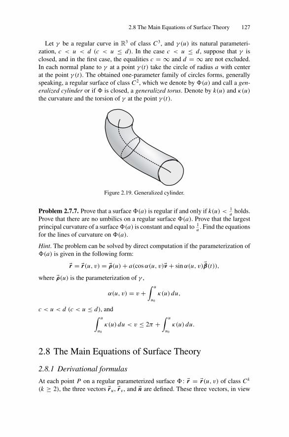
2.8 The Main Equations of Surface Theory 127
Let γ be a regular curve in R3 of class C3, and γ (u) its natural parameteri-zation, c < u < d (c < u ≤ d). In the case c < u ≤ d , suppose that γ isclosed, and in the first case, the equalities c = ∞ and d = ∞ are not excluded.In each normal plane to γ at a point γ (t) take the circle of radius a with centerat the point γ (t). The obtained one-parameter family of circles forms, generallyspeaking, a regular surface of class C2, which we denote by �(a) and call a gen-eralized cylinder or if � is closed, a generalized torus. Denote by k(u) and κ(u)
the curvature and the torsion of γ at the point γ (t).
Figure 2.19. Generalized cylinder.
Problem 2.7.7. Prove that a surface �(a) is regular if and only if k(u) < 1a holds.
Prove that there are no umbilics on a regular surface �(a). Prove that the largestprincipal curvature of a surface �(a) is constant and equal to 1
a . Find the equationsfor the lines of curvature on �(a).
Hint. The problem can be solved by direct computation if the parameterization of�(a) is given in the following form:
�r = �r(u, v) = �ρ(u) + a(cos α(u, v)�ν + sin α(u, v)�β(t)),
where �ρ(u) is the parameterization of γ ,
α(u, v) = v +∫ u
u0
κ(u) du,
c < u < d (c < u ≤ d), and∫ u
u0
κ(u) du < v ≤ 2π +∫ u
u0
κ(u) du.
2.8 The Main Equations of Surface Theory
2.8.1 Derivational formulas
At each point P on a regular parameterized surface � : �r = �r(u, v) of class Ck
(k ≥ 2), the three vectors �ru , �rv , and �n are defined. These three vectors, in view

128 2. Extrinsic Geometry of Surfaces in Three-dimensional Euclidean Space
of the regularity of �, are linearly independent and consequently form a basis.Thus, any other vector can be presented as a linear combination of �ru , �rv , and �n.Find the coefficients of this decomposition by the basis of the vectors �ruu , �ruv ,�rvv and �nu , �nv . Let
�ruu = �111�ru + �2
11�rv + A11�n,
�ruv = �112�ru + �2
12�rv + A12�n,
�rvv = �122�ru + �2
22�rv + A22�n, (2.109)
�nu = α11�ru + α12�rv,
�nv = α21�ru + α22�rv.
It is easiest to find the coefficients Ai j (i, j = 1, 2). We obtain the scalar productof the first three equations of (2.109) on �n:
A11 = 〈�ruu, �n〉 = L , A12 = 〈�ruv, �n〉 = M, A22 = 〈�rvv, �n〉 = N . (2.110)
For coefficients α11, α12 and α21, α22 we obtain a system of equations by takingthe scalar product of the last two equations of (2.109) with �ru and �rv:{
α11 E + α12 F = −Lα11 F + α12G = −M,
(2.111){α21 E + α22 F = −Mα21 F + α22G = −N .
(2.112)
From (2.111) and (2.112) we have
α11 = −LG + M F
EG − F2, α12 = L F − M E
EG − F2,
α21 = N F − MG
EG − F2, α22 = −N E + M F
EG − F2. (2.113)
It is interesting to note that for a coordinate system whose coordinate curves co-incide with the lines of curvature, equations (2.113) can be rewritten in the form
α11 = −k1 α12 = α21 = 0, α22 = −k2,
where k1, and k2 are the principal curvatures of � at a given point. We shall obtaina system of equations for the coefficients �i
jk , applying the scalar multiplicationof the first three equations of (2.109) on �ru and �rv:{
�111 E + �2
11 F = 〈�ruu, �ru〉 = 12 Eu
�111 F + �2
11G = 〈�ruu, �rv〉 = Fu − 12 Ev,
(2.114){�1
12 E + �212 F = 〈�ruv, �ru〉 = 1
2 Ev
�112 F + �2
12G = 〈�ruv, �rv〉 = 12 Gu,
(2.115){�1
22 E + �222 F = 〈�rvv, �ru〉 = Fv − 1
2 Gu
�122 F + �2
22G = 〈�rvv, �rv〉 = 12 Gv.
(2.116)
2.8 The Main Equations of Surface Theory 129
By the way, we have used the identities
〈�ruu, �rv〉 = − ∂
∂u〈�ru, �rv〉 − 〈�ru�ruv〉, 〈�rvv, �ru〉 = ∂
∂v〈�rv, �ru〉 − 〈�rv�ruv〉.
Solving the systems (2.114)–(2.116) we obtain
�111 =
12 EuG + 1
2 Ev F − F Fu
EG − F2, �2
11 = Fu E − 12 Ev E − 1
2 Eu F
EG − F2,
�112 =
12 EvG − 1
2 Gu F
EG − F2, �2
12 =12 Gu E − 1
2 Ev F
EG − F2, (2.117)
�122 = − 1
2 GuG − 12 Gv F + G Fv
EG − F2, �2
22 =12 Gv E + 1
2 Gu F − F Fv
EG − F2.
If the coordinate system (u, v) is orthogonal, i.e., F(u, v) = 0, then the formulasfor �i
jk (i, j, k = 1, 2) are essentially simplified:
�111 = Eu
2E, �2
11 = − Ev
2G, �1
12 = Ev
2E,
�212 = Gu
2G, �1
22 = − Gu
2E, �2
22 = Gv
2G.
(2.118)
The geometrical sense of the coefficients �ijk (i, j, k = 1, 2) will be cleared up
below, in Chapter 3. Now note only that they are expressed through the coeffi-cients of the first fundamental form and their first derivatives only. The coeffi-cients themselves are called the Christoffel symbols of the second kind. Finally,note that the derivational formulas (2.109) can be considered as a direct general-ization of the Frenet formulas for the space curves (see Chapter 1).
2.8.2 Gauss–Peterson–Codazzi Formulas
If E(λ1)2 +2F(λ1)(λ2)+G(λ2)2 and L(λ1)2 +2M(λ1)(λ2)+ N (λ2)2 are the firstand the second fundamental forms of a surface, then they cannot be taken arbi-trarily. There are definite relations between the coefficients of these fundamentalforms. These relations can be found based on the independence of the derivativesfrom the order of derivation. If a regular surface � belongs to class Ck (k ≥ 3)
and �r = �r(u, v) is its vector equation, then the following equations hold:
(�ruu)v = (�ruv)u, (�rvv)u = (�ruv)v, (�nu)v = (�nv)u .
If we substitute in these formulas the expressions for �ruu , �ruv , �rvv , �nu , �nv from(2.109), then the three vector equalities
(�111�ru + �2
11�rv + L �n)v = (�112�ru + �2
12�rv + M �n)u,
(�122�ru + �2
22�rv + N �n)u = (�112�ru + �2
12�rv + M �n)v,
(α11�ru + α12�rv)v = (α21�ru + α22�rv)u . (2.119)
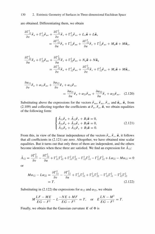
130 2. Extrinsic Geometry of Surfaces in Three-dimensional Euclidean Space
are obtained. Differentiating them, we obtain
∂�111
∂v�ru + �1
11�ruv + ∂�211
∂v�rv + �2
11�rvv + Lv �n + L �nv
= ∂�112
∂u�ru + �1
12�ruu + ∂�212
∂u�rv + �2
12�ruv + Mu �n + M �nu,
∂�122
∂u�ru + �1
22�ruu + ∂�222
∂u�rv + �2
22�ruv + Nu �n + N �nu
= ∂�112
∂v�ru + �1
12�ruv + ∂�212
∂v�rv + �2
12�rvv + Mv �n + M �nv,
∂α11
∂v�ru + α11�ruv + ∂α12
∂v�rv + α12�rvv
= ∂α21
∂u�ru + α21�ruu + ∂α22
∂u�rv + α22�ruv. (2.120)
Substituting above the expressions for the vectors �ruu , �ruv , �rvv and �nu , �nv from(2.109) and collecting together the coefficients at �ru , �ru , �n, we obtain equalitiesof the following form: ⎧⎨⎩
A11�ru + A12�rv + B1�n = 0,
A21�ru + A22�rv + B2�n = 0,
A31�ru + A32�rv + B3�n = 0.
(2.121)
From this, in view of the linear independence of the vectors �ru , �rv , �n, it followsthat all coefficients in (2.121) are zero. Altogether, we have obtained nine scalarequalities. But it turns out that only three of them are independent, and the othersbecome identities when these three are satisfied. We find an expression for A12:
A12 = ∂�211
∂v− ∂�2
12
∂u+ �1
11�212 + �2
11�222 − �1
12�211 − �2
12�212 + Lα22 − Mα12 = 0
or
Mα12 − Lα22 = ∂�211
∂v− ∂�2
12
∂u+ �1
11�212 + �2
11�222 − �1
12�211 − �2
12�212
= T . (2.122)
Substituting in (2.122) the expressions for α12 and α22, we obtain
ML F − M E
EG − F2− L
−N E + M F
EG − F2= T, or E
L N − M2
EG − F2= T .
Finally, we obtain that the Gaussian curvature K of � is
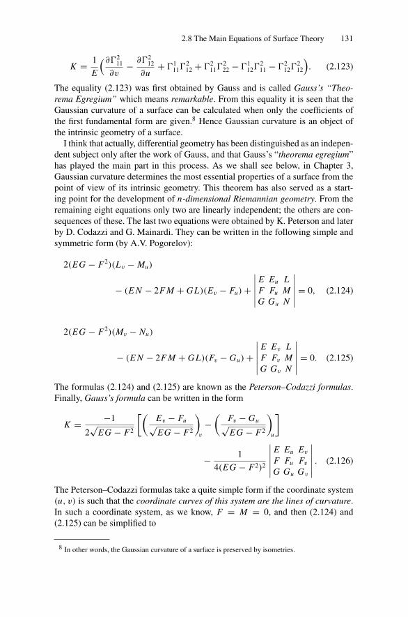
2.8 The Main Equations of Surface Theory 131
K = 1
E
(∂�211
∂v− ∂�2
12
∂u+ �1
11�212 + �2
11�222 − �1
12�211 − �2
12�212
). (2.123)
The equality (2.123) was first obtained by Gauss and is called Gauss’s “Theo-rema Egregium” which means remarkable. From this equality it is seen that theGaussian curvature of a surface can be calculated when only the coefficients ofthe first fundamental form are given.8 Hence Gaussian curvature is an object ofthe intrinsic geometry of a surface.
I think that actually, differential geometry has been distinguished as an indepen-dent subject only after the work of Gauss, and that Gauss’s “theorema egregium”has played the main part in this process. As we shall see below, in Chapter 3,Gaussian curvature determines the most essential properties of a surface from thepoint of view of its intrinsic geometry. This theorem has also served as a start-ing point for the development of n-dimensional Riemannian geometry. From theremaining eight equations only two are linearly independent; the others are con-sequences of these. The last two equations were obtained by K. Peterson and laterby D. Codazzi and G. Mainardi. They can be written in the following simple andsymmetric form (by A.V. Pogorelov):
2(EG − F2)(Lv − Mu)
− (E N − 2F M + GL)(Ev − Fu) +∣∣∣∣∣∣
E Eu LF Fu MG Gu N
∣∣∣∣∣∣ = 0, (2.124)
2(EG − F2)(Mv − Nu)
− (E N − 2F M + GL)(Fv − Gu) +∣∣∣∣∣∣
E Ev LF Fv MG Gv N
∣∣∣∣∣∣ = 0. (2.125)
The formulas (2.124) and (2.125) are known as the Peterson–Codazzi formulas.Finally, Gauss’s formula can be written in the form
K = −1
2√
EG − F2
[(Ev − Fu√EG − F2
)v
−(
Fv − Gu√EG − F2
)u
]
− 1
4(EG − F2)2
∣∣∣∣∣∣E Eu Ev
F Fu Fv
G Gu Gv
∣∣∣∣∣∣ . (2.126)
The Peterson–Codazzi formulas take a quite simple form if the coordinate system(u, v) is such that the coordinate curves of this system are the lines of curvature.In such a coordinate system, as we know, F = M = 0, and then (2.124) and(2.125) can be simplified to
8 In other words, the Gaussian curvature of a surface is preserved by isometries.
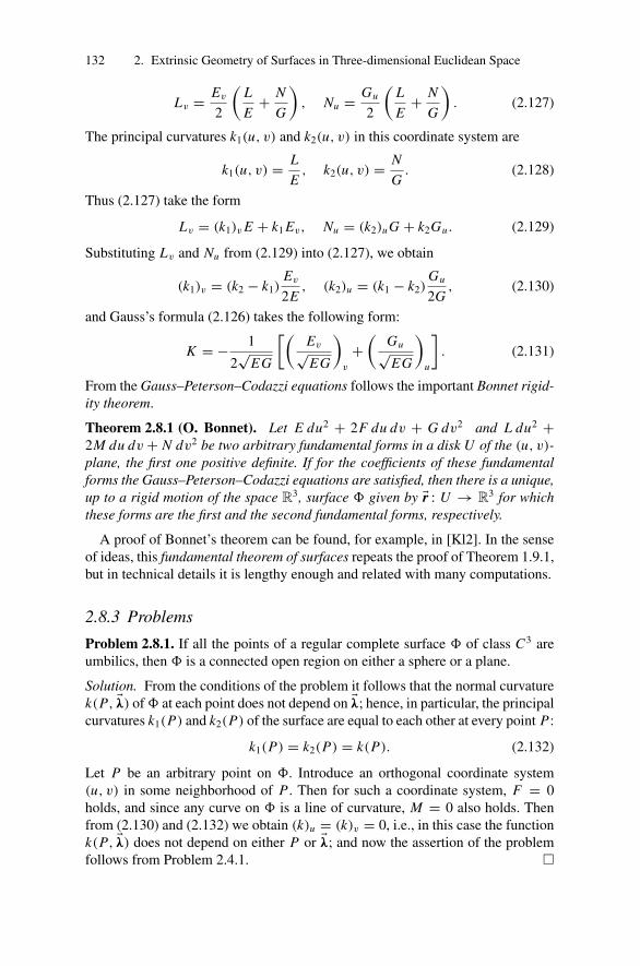
132 2. Extrinsic Geometry of Surfaces in Three-dimensional Euclidean Space
Lv = Ev
2
(L
E+ N
G
), Nu = Gu
2
(L
E+ N
G
). (2.127)
The principal curvatures k1(u, v) and k2(u, v) in this coordinate system are
k1(u, v) = L
E, k2(u, v) = N
G. (2.128)
Thus (2.127) take the form
Lv = (k1)v E + k1 Ev, Nu = (k2)uG + k2Gu . (2.129)
Substituting Lv and Nu from (2.129) into (2.127), we obtain
(k1)v = (k2 − k1)Ev
2E, (k2)u = (k1 − k2)
Gu
2G, (2.130)
and Gauss’s formula (2.126) takes the following form:
K = − 1
2√
EG
[(Ev√EG
)v
+(
Gu√EG
)u
]. (2.131)
From the Gauss–Peterson–Codazzi equations follows the important Bonnet rigid-ity theorem.
Theorem 2.8.1 (O. Bonnet). Let E du2 + 2F du dv + G dv2 and L du2 +2M du dv + N dv2 be two arbitrary fundamental forms in a disk U of the (u, v)-plane, the first one positive definite. If for the coefficients of these fundamentalforms the Gauss–Peterson–Codazzi equations are satisfied, then there is a unique,up to a rigid motion of the space R3, surface � given by �r : U → R3 for whichthese forms are the first and the second fundamental forms, respectively.
A proof of Bonnet’s theorem can be found, for example, in [Kl2]. In the senseof ideas, this fundamental theorem of surfaces repeats the proof of Theorem 1.9.1,but in technical details it is lengthy enough and related with many computations.
2.8.3 Problems
Problem 2.8.1. If all the points of a regular complete surface � of class C3 areumbilics, then � is a connected open region on either a sphere or a plane.
Solution. From the conditions of the problem it follows that the normal curvaturek(P, �λ) of � at each point does not depend on �λ; hence, in particular, the principalcurvatures k1(P) and k2(P) of the surface are equal to each other at every point P:
k1(P) = k2(P) = k(P). (2.132)
Let P be an arbitrary point on �. Introduce an orthogonal coordinate system(u, v) in some neighborhood of P . Then for such a coordinate system, F = 0holds, and since any curve on � is a line of curvature, M = 0 also holds. Thenfrom (2.130) and (2.132) we obtain (k)u = (k)v = 0, i.e., in this case the functionk(P, �λ) does not depend on either P or �λ; and now the assertion of the problemfollows from Problem 2.4.1. �
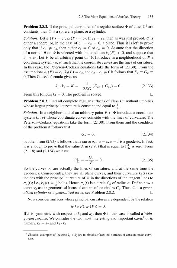
2.8 The Main Equations of Surface Theory 133
Problem 2.8.2. If the principal curvatures of a regular surface � of class C2 areconstants, then � is a sphere, a plane, or a cylinder.
Solution. Let k1(P) = c1, k2(P) = c2. If c1 = c2, then as was just proved, � iseither a sphere, or, in the case of c1 = c2 = 0, a plane. Thus it is left to proveonly that if c1 �= c2, then either c1 = 0 or c2 = 0. Assume that the directionof a normal �n on � is selected with the condition k2(P) > 0, and suppose thatc1 < c2. Let P be an arbitrary point on �. Introduce in a neighborhood of P acoordinate system (u, v) such that the coordinate curves are the lines of curvature.In this case, the Peterson–Codazzi equations take the form of (2.130). From theassumptions k1(P) = c1, k2(P) = c2, and c2 − c1 �= 0 it follows that Ev ≡ Gu ≡0. Then Gauss’s formula gives us
k1 · k2 = K = − 1
2EG(Evv + Guu) = 0. (2.133)
From this follows k1 = 0. The problem is solved. �Problem 2.8.3. Find all complete regular surfaces of class C3 without umbilicswhose largest principal curvature is constant and equal to 1
a .
Solution. In a neighborhood of an arbitrary point P ∈ � introduce a coordinatesystem (u, v) whose coordinate curves coincide with the lines of curvature. ThePeterson–Codazzi equations take the form (2.130). From them and the conditionof the problem it follows that
Gu ≡ 0, (2.134)
but then from (2.93) it follows that a curve σu : u = c, v = t is a geodesic. In fact,it is enough to prove that the value A in (2.93) that is equal to �1
22 is zero. From(2.118) and (2.134) we have
�122 = −Gu
E= 0. (2.135)
So the curves σu are actually the lines of curvature, and at the same time thegeodesics. Consequently, they are all plane curves, and their curvature k2(t) co-incides with the principal curvature of � in the directions of the tangent lines toσu(t); i.e., ku(t) = 1
a holds. Hence σu(t) is a circle Cu of radius a. Define now acurve γu as the geometrical locus of centers of the circles Cu . Thus, � is a gener-alized cylinder or a generalized torus; see Problem 2.8.2. �
Now consider surfaces whose principal curvatures are dependent by the relation
h(k1(P), k2(P)) = 0.
If h is symmetric with respect to k1 and k2, then � in this case is called a Wein-garten surface. We consider the two most interesting and important cases9 of h,namely, k1 + k2 and k1 · k2.
9 Classical examples of the case k1 + k2 are minimal surfaces and surfaces of constant mean curva-ture.
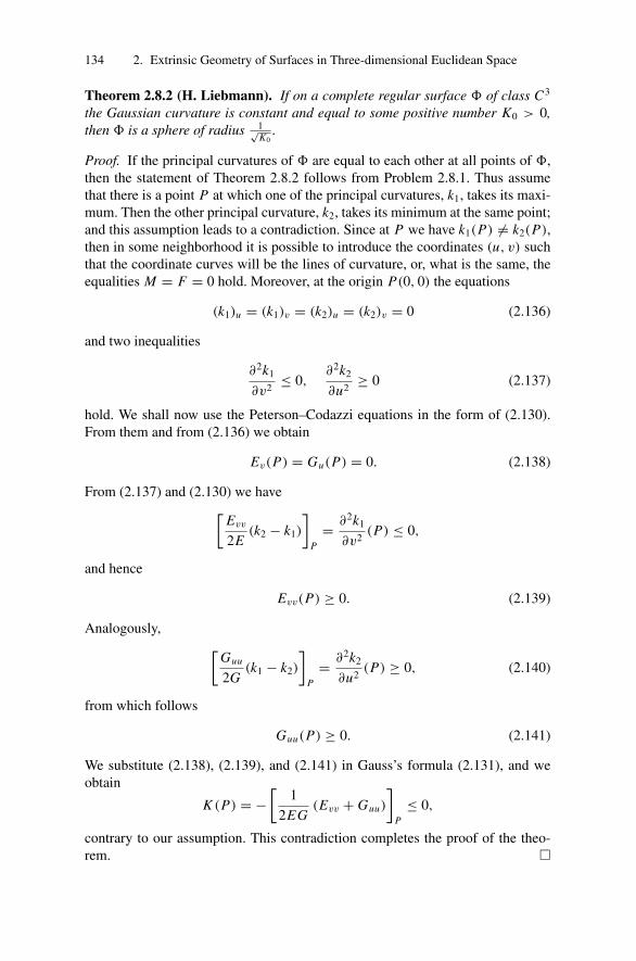
134 2. Extrinsic Geometry of Surfaces in Three-dimensional Euclidean Space
Theorem 2.8.2 (H. Liebmann). If on a complete regular surface � of class C3
the Gaussian curvature is constant and equal to some positive number K0 > 0,then � is a sphere of radius 1√
K0.
Proof. If the principal curvatures of � are equal to each other at all points of �,then the statement of Theorem 2.8.2 follows from Problem 2.8.1. Thus assumethat there is a point P at which one of the principal curvatures, k1, takes its maxi-mum. Then the other principal curvature, k2, takes its minimum at the same point;and this assumption leads to a contradiction. Since at P we have k1(P) �= k2(P),then in some neighborhood it is possible to introduce the coordinates (u, v) suchthat the coordinate curves will be the lines of curvature, or, what is the same, theequalities M = F = 0 hold. Moreover, at the origin P(0, 0) the equations
(k1)u = (k1)v = (k2)u = (k2)v = 0 (2.136)
and two inequalities
∂2k1
∂v2≤ 0,
∂2k2
∂u2≥ 0 (2.137)
hold. We shall now use the Peterson–Codazzi equations in the form of (2.130).From them and from (2.136) we obtain
Ev(P) = Gu(P) = 0. (2.138)
From (2.137) and (2.130) we have[Evv
2E(k2 − k1)
]P
= ∂2k1
∂v2(P) ≤ 0,
and hence
Evv(P) ≥ 0. (2.139)
Analogously, [Guu
2G(k1 − k2)
]P
= ∂2k2
∂u2(P) ≥ 0, (2.140)
from which follows
Guu(P) ≥ 0. (2.141)
We substitute (2.138), (2.139), and (2.141) in Gauss’s formula (2.131), and weobtain
K (P) = −[
1
2EG(Evv + Guu)
]P
≤ 0,
contrary to our assumption. This contradiction completes the proof of the theo-rem. �
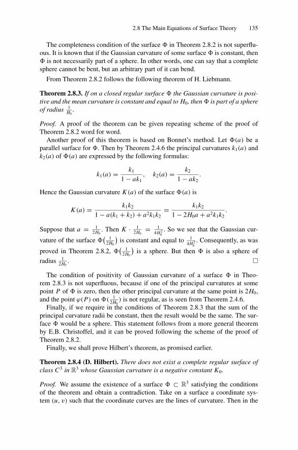
2.8 The Main Equations of Surface Theory 135
The completeness condition of the surface � in Theorem 2.8.2 is not superflu-ous. It is known that if the Gaussian curvature of some surface � is constant, then� is not necessarily part of a sphere. In other words, one can say that a completesphere cannot be bent, but an arbitrary part of it can bend.
From Theorem 2.8.2 follows the following theorem of H. Liebmann.
Theorem 2.8.3. If on a closed regular surface � the Gaussian curvature is posi-tive and the mean curvature is constant and equal to H0, then � is part of a sphereof radius 1
H0.
Proof. A proof of the theorem can be given repeating scheme of the proof ofTheorem 2.8.2 word for word.
Another proof of this theorem is based on Bonnet’s method. Let �(a) be aparallel surface for �. Then by Theorem 2.4.6 the principal curvatures k1(a) andk2(a) of �(a) are expressed by the following formulas:
k1(a) = k1
1 − ak1, k2(a) = k2
1 − ak2.
Hence the Gaussian curvature K (a) of the surface �(a) is
K (a) = k1k2
1 − a(k1 + k2) + a2k1k2= k1k2
1 − 2H0a + a2k1k2.
Suppose that a = 12H0
. Then K · 12H0
= 14H 2
0. So we see that the Gaussian cur-
vature of the surface �(
12H0
)is constant and equal to 1
4H 20
. Consequently, as was
proved in Theorem 2.8.2, �(
12H0
)is a sphere. But then � is also a sphere of
radius 12H0
. �
The condition of positivity of Gaussian curvature of a surface � in Theo-rem 2.8.3 is not superfluous, because if one of the principal curvatures at somepoint P of � is zero, then the other principal curvature at the same point is 2H0,and the point ϕ(P) on �( 1
2H0) is not regular, as is seen from Theorem 2.4.6.
Finally, if we require in the conditions of Theorem 2.8.3 that the sum of theprincipal curvature radii be constant, then the result would be the same. The sur-face � would be a sphere. This statement follows from a more general theoremby E.B. Christoffel, and it can be proved following the scheme of the proof ofTheorem 2.8.2.
Finally, we shall prove Hilbert’s theorem, as promised earlier.
Theorem 2.8.4 (D. Hilbert). There does not exist a complete regular surface ofclass C3 in R3 whose Gaussian curvature is a negative constant K0.
Proof. We assume the existence of a surface � ⊂ R3 satisfying the conditionsof the theorem and obtain a contradiction. Take on a surface a coordinate sys-tem (u, v) such that the coordinate curves are the lines of curvature. Then in the

136 2. Extrinsic Geometry of Surfaces in Three-dimensional Euclidean Space
notation of Theorem 2.8.2 (Liebmann), we obtain the system of equations, see(2.130),
(k1)v = (k2 − k1)Ev
2E, (k2)u = (k1 − k2)
Gu
2G. (2.142)
Assuming K0 = −1 and integrating system (2.142), we obtain
E = C1(u)
1 + k21(u, v)
, G = C2(v)
1 + k22(u, v)
.
The constants of integration C1(u), C2(v), without loss a generality, may be as-sumed to be 1. For this purpose it is enough to require that E(u, 0) = 1
1+k21(u,0)
and
G(0, v) = 11+k2
2(0,v), which one can always achieve. Thus, we obtain the equality
E = 1
1 + k21
, G = 1
1 + k22
.
But then, in view of k1k2 = −1,
E + G = 1
1 + k21
+ 1
1 + k22
= 2 + k21 + k2
2
1 + k21 + k2
2 + k21k2
2
= 2 + k21 + k2
2
2 + k21 + k2
2
= 1,
and hence we obtain √E = sin σ,
√G = cos σ.
From this, using (2.128), we find that
L = + sin σ cos σ, N = − sin σ cos σ.
Hence, a differential equation of asymptotic curves takes the form
(du + dv)(du − dv) = 0.
If we introduce new parameters p and q by the equalities
u = p − q, v = p + q,
then the new coordinate curves p = const and q = const will be the asymptoticcurves of the surface. The linear element of the surface will thus be presented bythe following expression:
ds2 = du2 sin2 σ + dv2 cos2 σ = dp2 + 2 dp dq cos σ + dq2.
From here, by the way, one may conclude that the opposite sides in a quadrangleformed from asymptotic curves are equal. Such nets of curves (for which E =G = 1) on arbitrary surfaces were investigated by the Russian mathematicianP.L. Tchebyshev in 1878. Such figures are formed by pulling a fishnet over a bentsurface.

2.8 The Main Equations of Surface Theory 137
If we apply Gauss’s formula (2.126) to the linear element expressed throughparameters p, q , then for an angle 2σ = ω formed by two asymptotic curves, weobtain the differential equation
∂2ω
∂p ∂q= sin ω. (2.143)
From here it is easy to deduce some simple corollaries; for example, for the areaof a surface,
F =∫∫
sin ω dp dq.
For the area of a quadrangle bounded by asymptotic curves p1 < p < p2, q1 <
q < q2, we obtain
F = ω(p1, q1) − ω(p1, q2) + ω(p2, q2) − ω(p2, q1),
or if we denote the inner angles by αk (see Figure 2.20 a),
F = α1 + α2 + α3 + α4 − 2π (0 < αk < π). (2.144)
This formula was first given by J.N. Hazzidakis.10 All known surfaces of constantnegative curvature, as for example a helicoid found by F. Minding, have singularlines. Therefore, Hilbert asked whether there exist unbounded and in any finitearea everywhere regular analytic surfaces with curvature K = −1. It turned outthat such surfaces cannot exist.
If such a surface existed, then its asymptotic curves would be in any finite areaeverywhere regular analytic curves; two asymptotic curves would pass througheach of its points with two different tangent lines, so that we could subordinate anangle between them to the condition 0 < ω < π . If we now accept that p and qare rectangular coordinates of a point in a plane, then we can put the points of oursurface in one-to-one correspondence with the points of the plane.
Figure 2.20. Tchebyshev net.
10 Uber einige Eigenschaften der Flachen mit konstantem Krummungsmasz, Crelles J., v. 88, 68–73,1880.
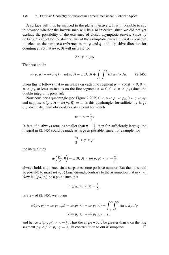
138 2. Extrinsic Geometry of Surfaces in Three-dimensional Euclidean Space
A surface will thus be mapped to the plane injectively. It is impossible to sayin advance whether the inverse map will be also injective, since we did not yetexclude the possibility of the existence of closed asymptotic curves. Since by(2.143), ω cannot be constant on any of the asymptotic curves, then it is possibleto select on the surface a reference mark, p and q , and a positive direction forcounting p, so that ω(p, 0) will increase for
0 ≤ p ≤ p2.
Then we obtain
ω(p, q) − ω(0, q) = ω(p, 0) − ω(0, 0) +∫ p
0
∫ q
0sin ω dp dq. (2.145)
From this it follows that ω increases on each line segment q = const > 0, 0 <
p < p2, at least as fast as on the line segment q = 0, 0 < p < p2 (since thedouble integral is positive).
Now consider a quadrangle (see Figure 2.20 b) 0 < p < p1 < p2, 0 < q < q1,and suppose ω(p2, 0) − ω(p1, 0) = ε. In this quadrangle, for sufficiently largeq1, obviously, there obviously exists a point for which
ω = π − ε
2.
In fact, if ω always remains smaller than π − ε2 , then for sufficiently large q, the
integral in (2.145) could be made as large as possible, since, for example, for
p1
2< q < p1
the inequalities
ω( p1
2, 0)
− ω(0, 0) < ω(p, q) < π − ε
2
always hold, and hence sin ω surpasses some positive number. But then it wouldbe possible to make ω(p, q) large enough, contrary to the assumption that ω < π .Now let (p0, q0) be a point such that
ω(p0, q0) < π − ε
2.
In view of (2.145), we obtain
ω(p2, q0) − ω(p0, q0) = ω(p2, 0) − ω(p0, 0) +∫ p2
p0
∫ q0
0sin ω dp dq
> ω(p2, 0) − ω(p1, 0) = ε,
and hence ω(p2, q0) > π − ε2 . Thus the angle would be greater than π on the line
segment p0 < p < p2; q = q0, in contradiction to our assumption. �
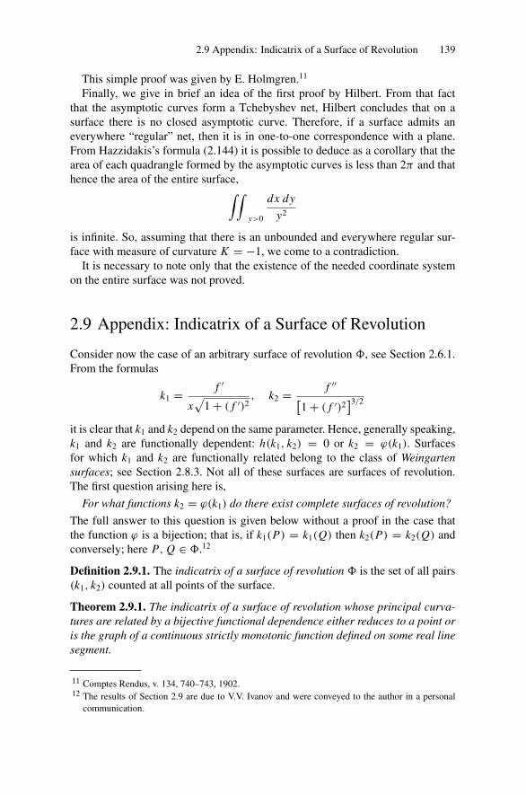
2.9 Appendix: Indicatrix of a Surface of Revolution 139
This simple proof was given by E. Holmgren.11
Finally, we give in brief an idea of the first proof by Hilbert. From that factthat the asymptotic curves form a Tchebyshev net, Hilbert concludes that on asurface there is no closed asymptotic curve. Therefore, if a surface admits aneverywhere “regular” net, then it is in one-to-one correspondence with a plane.From Hazzidakis’s formula (2.144) it is possible to deduce as a corollary that thearea of each quadrangle formed by the asymptotic curves is less than 2π and thathence the area of the entire surface,∫∫
y>0
dx dy
y2
is infinite. So, assuming that there is an unbounded and everywhere regular sur-face with measure of curvature K = −1, we come to a contradiction.
It is necessary to note only that the existence of the needed coordinate systemon the entire surface was not proved.
2.9 Appendix: Indicatrix of a Surface of Revolution
Consider now the case of an arbitrary surface of revolution �, see Section 2.6.1.From the formulas
k1 = f ′
x√
1 + ( f ′)2, k2 = f ′′[
1 + ( f ′)2]3/2
it is clear that k1 and k2 depend on the same parameter. Hence, generally speaking,k1 and k2 are functionally dependent: h(k1, k2) = 0 or k2 = ϕ(k1). Surfacesfor which k1 and k2 are functionally related belong to the class of Weingartensurfaces; see Section 2.8.3. Not all of these surfaces are surfaces of revolution.The first question arising here is,
For what functions k2 = ϕ(k1) do there exist complete surfaces of revolution?
The full answer to this question is given below without a proof in the case thatthe function ϕ is a bijection; that is, if k1(P) = k1(Q) then k2(P) = k2(Q) andconversely; here P, Q ∈ �.12
Definition 2.9.1. The indicatrix of a surface of revolution � is the set of all pairs(k1, k2) counted at all points of the surface.
Theorem 2.9.1. The indicatrix of a surface of revolution whose principal curva-tures are related by a bijective functional dependence either reduces to a point oris the graph of a continuous strictly monotonic function defined on some real linesegment.
11 Comptes Rendus, v. 134, 740–743, 1902.12 The results of Section 2.9 are due to V.V. Ivanov and were conveyed to the author in a personal
communication.
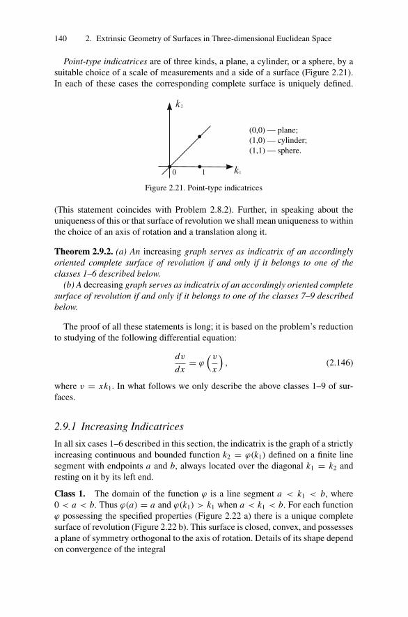
140 2. Extrinsic Geometry of Surfaces in Three-dimensional Euclidean Space
Point-type indicatrices are of three kinds, a plane, a cylinder, or a sphere, by asuitable choice of a scale of measurements and a side of a surface (Figure 2.21).In each of these cases the corresponding complete surface is uniquely defined.
(0,0) — plane;(1,0) — cylinder;(1,1) — sphere.
Figure 2.21. Point-type indicatrices
(This statement coincides with Problem 2.8.2). Further, in speaking about theuniqueness of this or that surface of revolution we shall mean uniqueness to withinthe choice of an axis of rotation and a translation along it.
Theorem 2.9.2. (a) An increasing graph serves as indicatrix of an accordinglyoriented complete surface of revolution if and only if it belongs to one of theclasses 1–6 described below.
(b) A decreasing graph serves as indicatrix of an accordingly oriented completesurface of revolution if and only if it belongs to one of the classes 7–9 describedbelow.
The proof of all these statements is long; it is based on the problem’s reductionto studying of the following differential equation:
dv
dx= ϕ
(v
x
), (2.146)
where v = xk1. In what follows we only describe the above classes 1–9 of sur-faces.
2.9.1 Increasing Indicatrices
In all six cases 1–6 described in this section, the indicatrix is the graph of a strictlyincreasing continuous and bounded function k2 = ϕ(k1) defined on a finite linesegment with endpoints a and b, always located over the diagonal k1 = k2 andresting on it by its left end.
Class 1. The domain of the function ϕ is a line segment a < k1 < b, where0 < a < b. Thus ϕ(a) = a and ϕ(k1) > k1 when a < k1 < b. For each functionϕ possessing the specified properties (Figure 2.22 a) there is a unique completesurface of revolution (Figure 2.22 b). This surface is closed, convex, and possessesa plane of symmetry orthogonal to the axis of rotation. Details of its shape dependon convergence of the integral
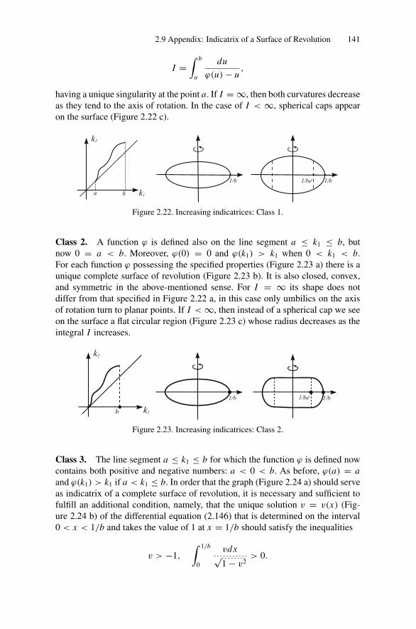
2.9 Appendix: Indicatrix of a Surface of Revolution 141
I =∫ b
a
du
ϕ(u) − u,
having a unique singularity at the point a. If I = ∞, then both curvatures decreaseas they tend to the axis of rotation. In the case of I < ∞, spherical caps appearon the surface (Figure 2.22 c).
Figure 2.22. Increasing indicatrices: Class 1.
Class 2. A function ϕ is defined also on the line segment a ≤ k1 ≤ b, butnow 0 = a < b. Moreover, ϕ(0) = 0 and ϕ(k1) > k1 when 0 < k1 < b.For each function ϕ possessing the specified properties (Figure 2.23 a) there is aunique complete surface of revolution (Figure 2.23 b). It is also closed, convex,and symmetric in the above-mentioned sense. For I = ∞ its shape does notdiffer from that specified in Figure 2.22 a, in this case only umbilics on the axisof rotation turn to planar points. If I < ∞, then instead of a spherical cap we seeon the surface a flat circular region (Figure 2.23 c) whose radius decreases as theintegral I increases.
Figure 2.23. Increasing indicatrices: Class 2.
Class 3. The line segment a ≤ k1 ≤ b for which the function ϕ is defined nowcontains both positive and negative numbers: a < 0 < b. As before, ϕ(a) = aand ϕ(k1) > k1 if a < k1 ≤ b. In order that the graph (Figure 2.24 a) should serveas indicatrix of a complete surface of revolution, it is necessary and sufficient tofulfill an additional condition, namely, that the unique solution v = v(x) (Fig-ure 2.24 b) of the differential equation (2.146) that is determined on the interval0 < x < 1/b and takes the value of 1 at x = 1/b should satisfy the inequalities
v > −1,
∫ 1/b
0
vdx√1 − v2
> 0.
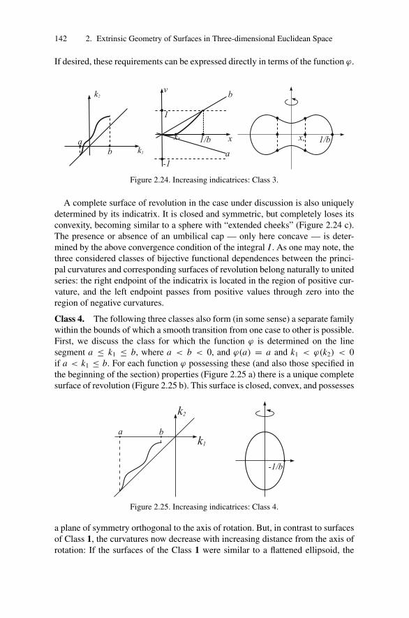
142 2. Extrinsic Geometry of Surfaces in Three-dimensional Euclidean Space
If desired, these requirements can be expressed directly in terms of the function ϕ.
Figure 2.24. Increasing indicatrices: Class 3.
A complete surface of revolution in the case under discussion is also uniquelydetermined by its indicatrix. It is closed and symmetric, but completely loses itsconvexity, becoming similar to a sphere with “extended cheeks” (Figure 2.24 c).The presence or absence of an umbilical cap — only here concave — is deter-mined by the above convergence condition of the integral I . As one may note, thethree considered classes of bijective functional dependences between the princi-pal curvatures and corresponding surfaces of revolution belong naturally to unitedseries: the right endpoint of the indicatrix is located in the region of positive cur-vature, and the left endpoint passes from positive values through zero into theregion of negative curvatures.
Class 4. The following three classes also form (in some sense) a separate familywithin the bounds of which a smooth transition from one case to other is possible.First, we discuss the class for which the function ϕ is determined on the linesegment a ≤ k1 ≤ b, where a < b < 0, and ϕ(a) = a and k1 < ϕ(k2) < 0if a < k1 ≤ b. For each function ϕ possessing these (and also those specified inthe beginning of the section) properties (Figure 2.25 a) there is a unique completesurface of revolution (Figure 2.25 b). This surface is closed, convex, and possesses
Figure 2.25. Increasing indicatrices: Class 4.
a plane of symmetry orthogonal to the axis of rotation. But, in contrast to surfacesof Class 1, the curvatures now decrease with increasing distance from the axis ofrotation: If the surfaces of the Class 1 were similar to a flattened ellipsoid, the
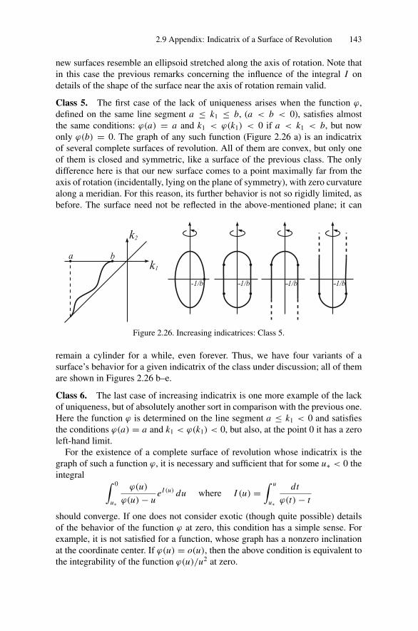
2.9 Appendix: Indicatrix of a Surface of Revolution 143
new surfaces resemble an ellipsoid stretched along the axis of rotation. Note thatin this case the previous remarks concerning the influence of the integral I ondetails of the shape of the surface near the axis of rotation remain valid.
Class 5. The first case of the lack of uniqueness arises when the function ϕ,defined on the same line segment a ≤ k1 ≤ b, (a < b < 0), satisfies almostthe same conditions: ϕ(a) = a and k1 < ϕ(k1) < 0 if a < k1 < b, but nowonly ϕ(b) = 0. The graph of any such function (Figure 2.26 a) is an indicatrixof several complete surfaces of revolution. All of them are convex, but only oneof them is closed and symmetric, like a surface of the previous class. The onlydifference here is that our new surface comes to a point maximally far from theaxis of rotation (incidentally, lying on the plane of symmetry), with zero curvaturealong a meridian. For this reason, its further behavior is not so rigidly limited, asbefore. The surface need not be reflected in the above-mentioned plane; it can
Figure 2.26. Increasing indicatrices: Class 5.
remain a cylinder for a while, even forever. Thus, we have four variants of asurface’s behavior for a given indicatrix of the class under discussion; all of themare shown in Figures 2.26 b–e.
Class 6. The last case of increasing indicatrix is one more example of the lackof uniqueness, but of absolutely another sort in comparison with the previous one.Here the function ϕ is determined on the line segment a ≤ k1 < 0 and satisfiesthe conditions ϕ(a) = a and k1 < ϕ(k1) < 0, but also, at the point 0 it has a zeroleft-hand limit.
For the existence of a complete surface of revolution whose indicatrix is thegraph of such a function ϕ, it is necessary and sufficient that for some u∗ < 0 theintegral ∫ 0
u∗
ϕ(u)
ϕ(u) − ueI (u) du where I (u) =
∫ u
u∗
dt
ϕ(t) − t
should converge. If one does not consider exotic (though quite possible) detailsof the behavior of the function ϕ at zero, this condition has a simple sense. Forexample, it is not satisfied for a function, whose graph has a nonzero inclinationat the coordinate center. If ϕ(u) = o(u), then the above condition is equivalent tothe integrability of the function ϕ(u)/u2 at zero.

144 2. Extrinsic Geometry of Surfaces in Three-dimensional Euclidean Space
The graph of the function satisfying the above-mentioned requirement (Fig-ure 2.27 a) is an indicatrix of the entire family of complete surfaces of revolution(Figure 2.27 b).
Figure 2.27. Increasing indicatrices: Class 6.
All of them are convex and are reminiscent of paraboloids by their shape, whichby the way, belong to the class of surfaces under discussion. Each surface ofour family runs to infinity with the determined inclination along a meridian. Theinclination can be either infinite (and thus horizontal cross-sections of a surfaceextend without bound), or a nonzero number. For each such inclination, there isexactly one representative member in the family of surfaces corresponding to thegiven indicatrix. It is curious to note that if at least one of the surfaces in thefamily belongs to a cap (the presence of which for the above reasons depends onthe nature of the approach of the left end of the indicatrix to the diagonal), thenall the others also belong.
2.9.2 Decreasing Indicatrices
Quite a different picture is obtained, when an indicatrix is a decreasing line. Inthe remaining examples it is the graph of the function ϕ that (besides what will betold about it in each concrete case) is defined on the bounded line segment withendpoints a < b ≤ 0, always including the point a, and is continuous and strictlydecreasing on it. Thus the graph is located entirely above the umbilical diagonal,sometimes intersecting it at one point.
Class 7. The domain of the function k2 = ϕ(k1) here is a line segment a ≤k1 < 0, so on it ϕ > 0 holds. Thus the left-hand limit of the function ϕ at thepoint 0 should be zero. Any such function determines a unique complete saddlesurface of revolution, homeomorphic to a cylinder with symmetric convex profilecurve having a catenoid-like shape. But some important details depend on theasymptotic character of the function ϕ at zero. To see this, consider the integrals
I (u) =∫ u
a
dt
ϕ(t) − tand J =
∫ 0
−1/a
v dx√1 − v2
.

2.9 Appendix: Indicatrix of a Surface of Revolution 145
The first of them is an increasing function on the line segment a ≤ u < 0, and itslimit for u → −0 will be denoted by the letter I . In the second integral, which alsocould be expressed explicitly through ϕ, the function v = v(x) means a uniquesolution of the differential equation (2.146), already familiar to us, existing on theinterval −1/a ≤ x < ∞ and satisfying the initial condition v(−1/a) = −1. Wehave three cases.
Case 1. Let I < ∞ and so J < ∞. Then if one completes the graph of a func-tion ϕ by one new point, attached to the origin (Figure 2.28 a), it serves as theindicatrix of an interesting surface whose profile curve is shown in Figure 2.28 b.
Figure 2.28. Decreasing indicatrices: Class 7, Case 1.
Case 2. Let I = ∞, but still J < ∞. In this case the indicatrix has no rightendpoint (Figure 2.29 a), and the surface is similar to the previous one, and differsfrom it in that it no longer sticks to two infinite rings compressing it, though itasymptotically tends to them (Figure 2.29 b).
Figure 2.29. Decreasing indicatrices: Class 7, Case 2.
Case 3. Let finally I = J = ∞. This means that the indicatrix rapidly approachesthe k1-axis (Figure 2.30 a). In this case the distance between the branches of theprofile curve (Figure 2.30 b) increases without bound while increasing its distancefrom the axis of rotation, but their inclination tends to a definite finite number. Itis expressed by the formula
1 − L√L(2 − L)
, where L = −1
a
∫ 0
a
ϕ(u)
ϕ(u) − ueI (u) du.
The values of the integral L fill the interval 0 < L ≤ 1, so the asymptotic incli-nation of the branches can be any number, starting from zero.

146 2. Extrinsic Geometry of Surfaces in Three-dimensional Euclidean Space
Figure 2.30. Decreasing indicatrices: Class 7, Case 3.
Class 8. A surface with a decreasing indicatrix can be periodic. Here we con-sider such a case. Let the function ϕ be determined on the line segment from ato b, where a < b < 0, and in addition to the above-mentioned general require-ments, the following conditions are satisfied: ϕ(a) > 0 > ϕ(b) > b. For theexistence of a complete surface of revolution whose indicatrix serves a graph ofsuch a function (Figure 2.31 a), it is necessary and sufficient for it to obey thefollowing equality:
I =∫ b
a
du
ϕ(u) − u= ln
a
b.
Then the surface (Figure 2.31 b) together with all its parameters is uniquely de-fined by its indicatrix.
Figure 2.31. Decreasing indicatrices: Class 8.
Class 9. The last case we should discuss is similar to the previous one in manyrespects, but differs from it in the moment of principle: it provides one more ex-ample of the lack of uniqueness. Here the function ϕ is determined on the sameline segment from a to b, where a < b < 0, but it now satisfies other conditions:ϕ(a) > 0 > ϕ(b) = b. The graph of such function a (Figure 2.32 a) serves as anindicatrix of a complete surface of revolution if and only if I < ln(a/b), whereI is the integral just considered. But now this surface is already not unique (Fig-ures 2.32 b – f). The reason is the following. The parallel farthest from the axis ofrotation consists of umbilics, and in the case I < ln(a/b), it appears as an entireumbilic layer. But also its one circle is enough for that after its achievement a sur-face could select the variant of further behavior. At each such moment it has twovariants — either to pass one more period repeating the previous form, or to curtailby a sphere. Thus there appears an infinite series of closed surfaces (Figures 2.32

2.10 Exercises to Chapter 2 147
b, c) similar to “pods of a peanut, containing some grains,” and their number canbe any natural number, but not smaller than two. If a surface once decides to stop,then we obtain two paraboloidal-type surfaces (i.e., homeomorphic to a plane) asshown in Figures 2.32 d, e. Finally, if a surface infinitely self-repeats the form,then it remains the same periodically pulsing cylindrical surface (Figure 2.32 f)that was seen in the previous class.
Figure 2.32. Decreasing indicatrices: Class 9.
2.10 Exercises to Chapter 2
Exercise 2.10.1. Write the parametric equations of (a) a twofold hyperbolic cylin-der, (b) a circular cylinder, (c) a circular cone.
Exercise 2.10.2. Write the equations of a surface of revolution with the axis O Z :(a) the torus obtained by a rotation of the circle x = a + b sin u, y = 0,
z = b sin u, 0 < b < a,(b) the pseudosphere obtained by rotation of the tractrix x = a sin u, y =
0, z = a(log tan u2 + cos u),
(c) the catenoid obtained by rotation of the catenary x = a cosh ua , y =
0, z = u.
Exercise 2.10.3. Show that the equations x = uu2+v2 , y = v
u2+v2 , z = 1u2+v2 and
x = u cos v, y = u sin v, z = u2 define the same surface.
Exercise 2.10.4. Prove that the surface x = a(uv+1)
u+v, y = b(u−v)
u+v, z = uv−1
u+v
is a onefold hyperboloid. What are the coordinate curves of the surface in thisparameterization?
Exercise 2.10.5. Given the surface x = a(u + v), y = b(u − v), z = u + a, findan explicit equation of the surface and prove that it is a hyperbolic paraboloid.
Exercise 2.10.6. Prove that the equation x = u + sin v, y = u + cos v, z = u + ais the equation of a cylinder.
Exercise 2.10.7. Write the equations of the tangent plane and a normal to thesurface (a) x2 + 2y2 − 3z2 − 4 = 0 at the point M(3, 1, −1), (b) x = u + v,y = u − v, z = uv at the point M(2, 1), (c) x = u cos v, y = u sin v, z = av ateach point.

148 2. Extrinsic Geometry of Surfaces in Three-dimensional Euclidean Space
Exercise 2.10.8. Write the equations of the tangent plane and a normal to thepseudosphere
x = a sin u cos v, y = a sin u sin v, z = a(
ln tanu
2+ cos u
).
Exercise 2.10.9. Show that all tangent planes to the surface z = x3 + y3 at thepoints M(α, −α, 0) form a set of planes.
Exercise 2.10.10. Find the first fundamental form of (a) a sphere⎧⎨⎩x = R cos u cos v,
y = R cos u sin v,
z = R sin u,
(b) a circular cone x = u cos v, y = u sin v, z = u , (c) the catenoid x = a cosh ua ,
y = u cos ua sin vz = u.
Exercise 2.10.11. Find the first fundamental form of each surface: (a) a cylinder,(b) a helicoid, (c) a pseudosphere.
Exercise 2.10.12. Let v = ln(u ± √u2 + 1) + C be the curves given on the right
helicoid x = u cos v, y = u sin v, z = 2v. Calculate the arc lengths of thesecurves between the points M1(1, 2) and M1(3, 4).
Exercise 2.10.13. Find the area of the quadrangle on the right helicoid x =u cos v, y = u sin v, z = av formed by the curves u = 0, u = a, v = 0,v = 1.
Exercise 2.10.14. Find the perimeter, inner angles, and the area of the curvilineartriangle
u = ± 12 avr , v = 1 on the helicoid x = u cos v, y = u sin v, z = −av.
Exercise 2.10.15. Find the second fundamental form of each surface: (a) cylinder,(b) sphere, (c) circular cone, (d) helicoid, (e) catenoid, (f) pseudosphere⎧⎨⎩
x = a sin u cos v,
y = a sin u sin v,
z = a(log tan u
2 + cos u).
Exercise 2.10.16. Find the principal curvatures (a) at the vertices of the twofoldhyperboloid x2
a2 − y2
b2 − z2
c2 −1 = 0, (b) of the surface z = xy at the point M(1, 1, 1).
Exercise 2.10.17. Find the principal curvatures and the principal vectors of eachsurface:
(a) z = xy at the point M(1, 1, 1), (b) x2
p + y2
p = 2z at the point M(0, 0, 0),
(c) x = u2 + v2, y = u2 − v2, z = uv at the point M(1, 1).

2.10 Exercises to Chapter 2 149
Exercise 2.10.18. Find the Gaussian curvature of each surface: (a) a sphere, (b) a(circular) cylinder, (c) a pseudosphere, (d) a catenoid, (e) a paraboloid x2
p + y2
p =2z, (f) a helicoid, (g) a torus.
Exercise 2.10.19. Calculate the mean curvature of a catenoid.
Exercise 2.10.20. Prove that the umbilics on the surface x = u2
2 + v, y = u + v2
2 ,z = uv lie on the curves u = v, u + v + 1 = 0.
Exercise 2.10.21. Find the lines of curvature on the following surfaces: (a) anarbitrary surface of revolution, (b) the surface x = u2 + v2, y = u2 − v2, z = v.
Exercise 2.10.22. Find the lines of curvature on each surface: (a) x = u2 + v2,y = u2 −v2, z = v, (b) x = 3u2 −u3 +3uv2, y = u2 −3u2v−3v, z = 3(u2 −v2).
Exercise 2.10.23. Prove that the curve x = 21+t , y = 2
1−t , z = t is an asymptoticcurve on the surface z = 1
x2 − 1y2 .
Exercise 2.10.24. Find the asymptotic curves of a right helicoid.
Exercise 2.10.25. Find the geodesic curvature of each curve:
(a) a circle of radius r on a sphere of radius R,
(b) a helix u = c, v = t on a helicoid x = u cos v, y = u sin v, z = u.
Exercise 2.10.26. Find the geodesic curvature of the curves u = const and v =const on a surface x = u cos v, y = y sin v, z = f (v).
Exercise 2.10.27. Prove that if no external forces act on a particle moving alonga surface, then it will move along a geodesic.
Exercise 2.10.28. Prove that every straight line on a surface is a geodesic.
Exercise 2.10.29. Prove that a geodesic is also a line of curvature if and only if itis a straight line.
Exercise 2.10.30. Prove that a geodesic is also an asymptotic curve if and only ifit is a plane curve.
Exercise 2.10.31. Two surfaces touch each other along a curve L . Prove that if Lis a geodesic on one of the surfaces, then it is also a geodesic on the other surface.
Exercise 2.10.32. Find the geodesics of (1) a cylindrical surface, (2) a circularcone, (3) a Mobius strip, (4) a flat torus, (5) a Klein bootle.
Hint. The surfaces (4), (5) are obtained from a square in the plane with the stan-dard metric after gluing the pair(s) of its sides with corresponding orientation.
Exercise 2.10.33. Prove that the meridians of a surface of revolution are itsgeodesics.
150 2. Extrinsic Geometry of Surfaces in Three-dimensional Euclidean Space
Exercise 2.10.34. Prove that a parallel of a surface of revolution is also itsgeodesic if and only if a tangent line to a meridian passing through a point isparallel to the axis of rotation.
Exercise 2.10.35. Find the geodesics on (a) a right helicoid: x = u cos v, y =u sin v, z = u, (b) a pseudosphere.
Exercise 2.10.36. Prove that the only minimal surfaces of revolution are a planeand a catenoid.
Exercise 2.10.37. Prove that among all ruled surfaces, only a plane and a catenoidare minimal.
Exercise 2.10.38.∗Let γ be a closed geodesic without points of self-intersectionon a closed convex surface. Prove that the spherical image of γ divides a sphereinto two parts with equal areas.

3Intrinsic Geometry of Surfaces
In this chapter the foundations of intrinsic geometry of a two-dimensional surfaceare introduced. The material is presented in such a form that all statements otherthan the Gauss–Bonnet theorem can be generalized almost word for word to themultidimensional case. So, this chapter can be considered as an introduction tothe theory of n-dimensional Riemannian manifolds.
3.1 Introducing Notation
The local coordinates (u, v) of some parameterization of a surface � will be writ-ten as (u1, u2), the vectors �ru1(u1, u2) and �ru2(u1, u2) by �r1 and �r2. Denote the co-efficients of the first fundamental form by gik (i, k = 1, 2), where gik = 〈�r i , �rk〉;the elements of the inverse matrix to {gi j } by gi j ; the coordinates of the vector�λ = λ1�r1 + λ2�r2 in a local basis �r1, �r2 by λ1, λ2. Introduce the magnitudes,called the Christoffel symbols of the first kind,
� jk,l = 1
2
(∂g jl
∂uk+ ∂gkl
∂u j− ∂g jk
∂ul
)(i, j, k = 1, 2), (3.1)
and the Christoffel symbols of the second kind by the formula
�ijk =
2∑l=1
� jk,l gli (i, j, k = 1, 2). (3.2)
The derivational formulas (2.109) in this notation take the form

152 3. Intrinsic Geometry of Surfaces
∂�r i
∂u j= �r i j =
2∑k=1
�ki j �rk + Ai j �n (i, j = 1, 2), (3.3)
where �n is a normal to �, and Ai j are the coefficients of the second fundamentalform. The Gaussian curvature K of � is expressed through the coefficients of thefirst fundamental form by the formula, see (2.123),
K = 1
g11
(∂�2
11
∂u2− ∂�2
11
∂u1+ �1
11�212 + �2
11�222 − �1
12�211 − �2
12�212
). (3.4)
If the equations of a curve c(t) in local coordinates (u1, u2) are given by thefunctions (u1(t), u2(t)), then the tangent vector to c(t), which is equal to (u1)′�r1+(u2)′�r2, is denoted by c(t). Later on, we will agree that if in any term the sameindex is written twice, one time up and the second time down, then it in fact occursas a summation with respect to this index. For example, (�µ, �λ) = gi jλ
iµ j , �ijk =
gil� jk,l , and so on.
3.2 Covariant Derivative of a Vector Field
Let �λ(t) ∈ T �c(t) be a differentiable vector field along a smooth curve c(t) on aregular surface � of class C3. Take the derivative d
dt�λ of this vector field at a point
c(t). In the general case, ddt
�λ does not belong to the tangent plane T �c(t). Define
the covariant derivative Ddt
�λ of the vector field �λ along c(t) as the orthogonal
projection of ddt
�λ onto T �c(t). From this definition it follows that
D
dt�λ = d
dt�λ −
⟨d
dt�λ, �n
⟩�n, (3.5)
where �n is a normal to � at c(t). To find an analytical expression for Ddt
�λ in
local coordinates, let �λ(t) = λ1(t)�r1(t) + λ2(t)�r2(t), and let c(t) be given by theequations u1 = u1(t), u2 = u2(t). From this notation we obtain
d
dt�λ = dλ1
dt�r1 + dλ2
dt�r2 + λ1
(�r11
du1
dt+ �r12
du2
dt
)+ λ2
(�r21
du1
dt+ �r22
du2
dt
).
We now express �r1i and �r2 j through �r1, �r2 and �n by derivational formulas (3.3),obtaining
d
dt�λ =
(dλ1
dt+ �1
i jλi du j
dt
)�r1 +
(dλ2
dt+ �2
i jλi du j
dt
)�r2 + A�n. (3.6)
From (3.6) it is seen that 〈 ddt
�λ, �n〉 = A. Therefore,
D
dt�λ =
(dλ1
dt+ �1
i jλi du j
dt
)�r1 +
(dλ2
dt+ �2
i jλi du j
dt
)�r2 (3.7)
3.3 Parallel Translation of a Vector along aCurve on a Surface 153
and (D
dt�λ)k
= dλk
dt+ �k
i jλi du j
dt(k = 1, 2). (3.8)
Remark 3.2.1. Sometimes it is useful to use Ddt
�λ|c(t) instead of the notation Ddt
�λ,indicating explicitly that the covariant derivative is taken along c(t).
Remark 3.2.2. In the definition of covariant derivative of a vector field �λ(t) alongc(t) we have used the circumstance that the surface � lies in R3. However, (3.7),(3.8), and (3.3) show that for a given curve c(t) and the vector field �λ(t) thecoordinates of a vector field D
dt�λ are expressed only through the coefficients of
the first fundamental form, their first-order derivatives, and the coordinates of �λ.Thus one can say that the covariant derivative of a vector field along a curve isan object of intrinsic geometry.
3.3 Parallel Translation of a Vector along aCurve on a Surface
Definition 3.3.1. A vector field �λ(t) along a curve c(t) on a surface � is called afield of parallel vectors if D
dt�λ(t)|c(t) ≡ 0.
Definition 3.3.2. We say that a vector �λ1 at a point c(t1) is obtained from a vector�λ0 at a point c(t0) by a parallel translation along c(t) (t0 ≤ t ≤ t1) if there isa field of parallel vectors �λ(t) (t0 ≤ t ≤ t1) along c(t) for which �λ(t0) = �λ0,�λ(t1) = �λ1.
If a curve c(t) lies entirely in one coordinate neighborhood, then for expressingthe coordinates λ1
1, λ21 of a vector �λ1 through coordinates λ1
0, λ20 of a vector �λ0, in
view of Definition 3.3.2, we need to solve the system, see (3.8),
dλk
dt+ �k
i jλi du j
dt= 0 (k = 1, 2) (3.9)
with initial conditions λ1(t0) = λ10, λ
2(t0) = λ20 and to set λ1
1 = λ1(t1), λ21 =
λ2(t1). The existence and uniqueness of a solution of the system (3.9) for arbitraryinitial conditions and for any t follow from a theorem about systems of ordinarydifferential equations.
If c(t) does not lie entirely in one coordinate neighborhood, then we divide itonto a finite number of arcs, each of which belongs to some coordinate neighbor-hood, and then produce a parallel translation along each part in consecutive order.Parallel translation of a vector can also be defined along a piecewise smooth curveas consecutive parallel translations along each smooth part. Note that a paralleldisplacement of a vector on a surface is defined as a parallel translation along agiven curve. Thus, in general, the result of a parallel translation depends on the
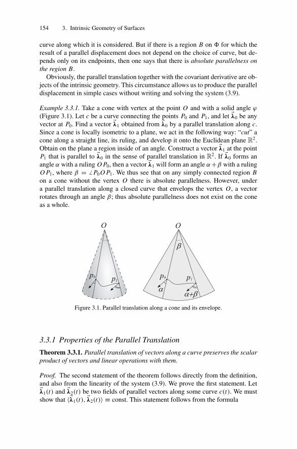
154 3. Intrinsic Geometry of Surfaces
curve along which it is considered. But if there is a region B on � for which theresult of a parallel displacement does not depend on the choice of curve, but de-pends only on its endpoints, then one says that there is absolute parallelness onthe region B.
Obviously, the parallel translation together with the covariant derivative are ob-jects of the intrinsic geometry. This circumstance allows us to produce the paralleldisplacement in simple cases without writing and solving the system (3.9).
Example 3.3.1. Take a cone with vertex at the point O and with a solid angle ϕ
(Figure 3.1). Let c be a curve connecting the points P0 and P1, and let �λ0 be anyvector at P0. Find a vector �λ1 obtained from �λ0 by a parallel translation along c.Since a cone is locally isometric to a plane, we act in the following way: “cut” acone along a straight line, its ruling, and develop it onto the Euclidean plane R2.Obtain on the plane a region inside of an angle. Construct a vector �λ1 at the pointP1 that is parallel to �λ0 in the sense of parallel translation in R2. If �λ0 forms anangle α with a ruling O P0, then a vector �λ1 will form an angle α+β with a rulingO P1, where β = � P0 O P1. We thus see that on any simply connected region Bon a cone without the vertex O there is absolute parallelness. However, undera parallel translation along a closed curve that envelops the vertex O , a vectorrotates through an angle β; thus absolute parallelness does not exist on the coneas a whole.
Figure 3.1. Parallel translation along a cone and its envelope.
3.3.1 Properties of the Parallel Translation
Theorem 3.3.1. Parallel translation of vectors along a curve preserves the scalarproduct of vectors and linear operations with them.
Proof. The second statement of the theorem follows directly from the definition,and also from the linearity of the system (3.9). We prove the first statement. Let�λ1(t) and �λ2(t) be two fields of parallel vectors along some curve c(t). We mustshow that 〈�λ1(t), �λ2(t)〉 ≡ const. This statement follows from the formula
3.3 Parallel Translation of a Vector along aCurve on a Surface 155
d
dt
⟨�λ1, �λ2
⟩=⟨
D
dt�λ1, �λ2
⟩+⟨�λ1,
D
dt�λ2
⟩. (3.10)
Let us prove it:d
dt〈�λ1, �λ2〉 =
⟨d
dt�λ1, �λ2
⟩+⟨�λ1,
d
dt�λ2
⟩.
From the definition of covariant derivative it follows that⟨
ddt
�λ1, �λ2⟩ = ⟨
Ddt
�λ1, �λ2⟩
and⟨�λ1,
ddt
�λ2⟩ = ⟨�λ1,
Ddt
�λ2⟩, from which follows (3.10). The statement of the the-
orem may be also proven by direct use of (3.9):
〈�λ1, �λ2〉 = gi jλi1λ
j2,
d
dt
(gi jλ
i1λ
j2
) = ∂gi j
∂uk
duk
dtλi
1λj2 + gi j
dλi1
dtλ
j2 + gi jλ
i1
dλj2
dt.
Substitute here dλi1
dt and dλj2
dt from (3.9), and then use (3.7) and (3.8). We obtain
d
dt〈�λ1, �λ2〉 = ∂gi j
∂uk
duk
dtλi
1λj2 − gi j�
ipkλ
p1
duk
dtλ
j2 − gi j�
jpkλ
p2
duk
dtλi
1
= ∂gi j
∂uk
duk
dtλi
1λj2 − �pk, jλ
p1 λ
j2
duk
dt− �pk,iλ
p2 λi
1duk
dt
= ∂gi j
∂ukλi
1λj2
duk
dt− 1
2
(∂gpi
∂uk+ ∂gkj
∂u p− ∂gpk
∂u j
)λ
p1 λ
j2
duk
dt
− 1
2
(∂gpi
∂uk+ ∂gkj
∂u p− ∂gpk
∂u j
)λi
1λp2
duk
dt
=[∂gi j
∂uk− 1
2
(∂gi j
∂uk+ ∂gkj
∂ui− ∂gik
∂u j
)− 1
2
(∂gi j
∂uk+ ∂gki
∂u j− ∂g jk
∂ui
)]· λi
1λj2
duk
dt= 0.
Thus based on the notion of covariant derivative of a vector field we can definethe notion of a parallel translation of a vector along a curve.
Conversely, we can define the covariant derivative of a vector field from thenotion of parallel translation of a vector along a curve. Indeed, let c(t) be a curveand �λ(t) a vector field along c(t). Take two vectors �λ(t) and λ(t + �t) at a pointc(t) and assume that λ(t +�t) is obtained from �λ(t +�t) by a parallel translationalong the arc c(t + �t)c(t) of a curve c(t). Then define
D
dt�λ|c = lim
�t→0
λ(t + �t) − �λ(t)
�t. (3.11)
Note that if a parallel translation of a vector in a local coordinates is defined by(3.9), then (3.8) can be deduced from (3.11). The proof of this statement is left tothe reader as an exercise. �

156 3. Intrinsic Geometry of Surfaces
3.4 Geodesics
In this section we continue the study the geodesics. It turns out that the propertiesof geodesics imitate the properties of straight lines in a plane as far as possible.One of the characteristic properties of a straight line in a plane is that a vectortangent to it stays tangent under parallel translation. Define a geodesic on a surface� as a curve with the same property.
3.4.1 Definition of Geodesics and Their Equations
Let γ (t) be a twice continuously differentiable curve on a regular surface � ofclass C2.
Definition 3.4.1. A curve γ (t) is called a geodesic on a surface � if the vectorfield γ (t) is a field of parallel vectors along γ (t).
We deduce the equations of geodesics in local coordinates. If the equations ofγ (t) are u1 = u1(t), u2 = u2(t), then the vector γ (t) has coordinates du1
dt , du2
dt .Consequently, from (3.8) follows(
D
dtγ
)k
= d2uk
dt2+ �k
i j
dui
dt
du j
dt(k = 1, 2),
and we obtain the equations of geodesics
d2uk
dt2+ �k
i j
dui
dt
du j
dt= 0 (k = 1, 2). (3.12)
Note that from our definition of geodesic it follows that the parameter t is thecanonical parameter, i.e., it is proportional to the arc length. In fact, since γ (t) isa field of parallel vectors, then from Theorem 3.3.1 it follows that |γ (t)| = c and
s =∫ t
0|γ (t)| dt = ct. (3.13)
Example 3.4.1. We find all geodesics on a cylinder with one more method. Asis seen from the definition of geodesics or directly from the system (3.12), thegeodesics under an isometric (or locally isometric) map of one surface onto otheralso turn into geodesics. Use this property for finding the geodesics on a circularcylinder of radius R. Cutting the cylinder along its ruling and developing it onto aplane, we obtain in the plane a strip of width 2π R between parallel straight linesa1 and a2. However, it is more convenient to do the following. Denote by �d avector orthogonal to a1 and of length 2π R. Take an arbitrary point P inside thestrip and identify with it all points in the plane that can be obtained by paralleldisplacement of P by a vector multiple of the vector �d. This identification allowsus to build a local isometry of the plane onto the cylinder (a covering map). Underthis map any straight line in the plane will turn into some geodesic on the cylinder,
3.4 Geodesics 157
and all geodesics on the cylinder can be thus obtained. This circumstance allowsus to find all geodesics on the cylinder. Straight lines that are parallel to a1 turninto rulings of the cylinder; straight lines that are orthogonal to a1 turn into closedgeodesics (parallels on a cylinder); and straight lines that are oblique to a1 turninto helices on the cylinder. Thus, the geodesics on a cylinder are exactly therulings, parallels, and helices.
Problem 3.4.1. Study the behavior of geodesics on a circular cone.
We prove now that the definitions of geodesics given in Chapters 2 and 3 areequivalent. Let γ (s) be a length-parameterized curve. Then D
ds γ = 0 means thatdds γ = �ν is a vector parallel to �n, and conversely, if the vector d
ds γ is parallel to�n, then D
ds γ = 0.
3.4.2 Exponential Map. Properties of an Exponential Mapand Local Properties of Geodesics
The system (3.12) is a system of second-order ordinary differential equations,solved with respect to the highest derivatives. Therefore, the next lemma followsfrom well-known theorems on the existence and uniqueness of solutions of sys-tems of ordinary differential equations and the continuous dependence of theirsolutions on initial values.
Lemma 3.4.1. For each point P on a surface � there are a neighborhood U ofP and a real number εP > 0 such that for every point Q ∈ U and an ar-bitrary vector �λ ∈ T �Q whose length is smaller than εP there is a uniquegeodesic γ (Q, �λ, t) (−1 < t < 1) satisfying the conditions γ (Q, �λ, 0) = Q,γ (Q, �λ, 0) = �λ.
From our notation and from (3.13) follows the equality
γ (Q, t · �λ, 1) = γ (Q, �λ, t). (3.14)
For some point Q and some vector �λ ∈ T �Q let there be a geodesic γ (Q, �λ, t)(0 ≤ t ≤ 1). Denote by expQ
�λ the point γ (Q, �λ, 1):
expQ�λ = γ (Q, �λ, 1). (3.15)
In view of Lemma 3.4.1, for each point Q ∈ � and each vector �λ ∈ T �Q whoselength is not greater than εQ there is a geodesic γ (Q, �λ, t) for 0 ≤ t ≤ 1. Conse-quently, (3.15) defines some map from an open disk of radius εQ with center at Qin the plane T �Q into �. This mapping is called an exponential map.
Problem 3.4.2. Describe the exponential map of a tangent plane on a sphere ofradius R. Find all critical points of this map.
158 3. Intrinsic Geometry of Surfaces
Lemma 3.4.2. The rank of the exponential map expQ�λ at the point Q is 2.
Proof. Let the equations of geodesics γ (Q, �λ, t) in local coordinates u1, u2 be
u1 = f 1(λ1, λ2, t), u2 = f 2(λ1, λ2, t).
Then the mapping expQ�λ is given by the functions f 1(λ1, λ2, 1), f 2(λ1, λ2, 1).
By the definition of a geodesic γ (Q, �λ, t),
d f i
dt
∣∣∣t=0
= λi (i = 1, 2). (3.16)
But in view of (3.14), the following identity holds:
f i (λ1, λ2, t) = f i (tλ1, tλ2, 1) (i = 1, 2). (3.17)
Differentiating the identity (3.17) by t and assuming t = 0, we obtain
d f i
dt(λ1, λ2, t)
∣∣∣t=0
= ∂ f i (0, 0, 1)
∂λ1λ1 + ∂ f i (0, 0, 1)
∂λ2λ2 (i = 1, 2). (3.18)
Now from (3.16) and (3.18) it follows that the Jacobian matrix of the mappingexpQ at the point Q is the unit matrix. �
From Lemmas 3.4.1 and 3.4.2 we shall deduce the main lemma of this section.
Lemma 3.4.3. For each point Q ∈ � there is a neighborhood WQ and a real εQ
such that for any two points Q1 ∈ WQ and Q2 ∈ WQ there is a unique geodesicγ (Q1, Q2, t) (0 ≤ t ≤ 1) joining Q1 and Q2 and of length not greater than εQ .
Proof. Let UQ and εQ be the neighborhood and real number obtained in Lemma3.4.1. Denote by A(UQ, εQ) the set of pairs (R, �λ), where R ∈ UQ and �λ ∈ T �R .Introduce coordinates on a set A by corresponding to each element (R, �λ) of theset A(UQ, εQ) the real numbers u1, u2, λ1, λ2, where u1, u2 are local coordinatesof the point R, and λ1, λ2 are the coordinates of �λ in a local basis of the planeT �R . Then define the set B = UQ × UQ . Also introduce coordinates in theset B by corresponding to each element (Q1, Q2) of the set B the real numbersx1, x2, y1, y2, where x1, x2 are local coordinates of the point Q1, and y1, y2 arelocal coordinates of the point Q2. Define a map f : A → B in the following way:correspond the pair (R, �λ) of A to the pair (R, expR
�λ) of B.(α). Prove that the rank of the map f at the point (Q, 0) is maximal, i.e., equal
to 4. By the notation of the previous lemma, the map f can be rewritten in thefollowing form:
x1 = u1, x2 = u2, y1 = f 1(u1, u2, λ1, λ2, 1),
y2 = f 2(u1, u2, λ1, λ2, 1).(3.19)
3.4 Geodesics 159
From (3.19) it is seen that the value of the determinant of the Jacobi matrix of
the map f at the point Q is equal to the value of the determinant∣∣∣ ∂ f 1/∂λ1 ∂ f 1/∂λ2
∂ f 2/∂λ1 ∂ f 2/∂λ2
∣∣∣derived for λ1 = λ2 = 0. The value 1 of the last determinant was calculated inLemma 3.4.2. The statement (α) is proven.
Continuing, we deduce from the inverse function theorem the existence of aneighborhood WQ and a real εQ such that the map f is a diffeomorphism of theset A(WQ, εQ) onto B. Let C = f(A). Take a neighborhood WQ of the pointQ such that WQ × WQ ⊂ C . Then the neighborhood WQ and εQ satisfy all therequirements of the lemma. �
By the way, we have proved that the coordinates of the point γ (Q1, Q2, t) andthe function l(Q1, Q2), the length of the geodesic γ (Q1, Q2, t), smoothly dependon the coordinates of the points Q1 and Q2 for Q1 �= Q2.
Example 3.4.2. For a sphere S2R of radius R in R3, any circular neighborhood WP
of radius ε with center at an arbitrary point P has all the properties given inLemma 3.4.3 if ε < 1
2π R. Indeed, recall that the geodesics on a sphere are thearcs of great circles. If P1 ∈ WP and P2 ∈ WP , then for ε < 1
2π R the pointsP1, P2 and the center O of the sphere lie on the same straight line. Pass a planethrough them. This plane intersects the sphere in a great circle, which, by theconstruction, is uniquely defined by the points P1 and P2, and the shortest arc ofthis circle lies entirely in WP and its length is smaller than ε.
Problem 3.4.3. Prove that for a circular cylinder of radius R any circular neigh-borhood WP of radius ε with center at the point P has all the properties fromLemma 3.4.3 if ε < 1
2π R.
3.4.3 Parallel Translation and Geodesic Curvature of a Curve
The geodesic curvature kg of an arbitrary curve on a surface was defined in Sec-tion 2.7.3. Now we shall give another (equivalent) definition of kg using the notionof parallel translation of a vector along a curve. Let c(t) be a parameterization ofa curve c, and t an arc length parameter. Take two vectors c(t) and c′
(t + �t)at a point c(t), where the vector c′
(t + �t) is obtained from c(t + �t) by paral-lel translation along the arc c(t + �t)c(t) of the curve c. Denote by �ψ(�t, t)the angle between c(t) and c′
(t + �t). Define now the geodesic curvature by theformula
kg = lim�t→0
�ψ(�t, t)
�t. (3.20)
Theorem 3.4.1. For any regular curve c(t) of class C2, the geodesic curvatureexists and is
kg =∣∣∣ D
dtc∣∣∣, (3.21)
where t is an arc length parameter.

160 3. Intrinsic Geometry of Surfaces
Proof. Since c(t) and c′(t + �t) are unit vectors, then 2 sin �ψ
2 = |c′(t + �t) −
c(t)|. Hence
kg = lim�t→0
�ψ
�t= lim
�t→0
�ψ
2 sin �ψ
2
· lim�t→0
|c′(t + �t) − c(t)|
�t=∣∣∣∣ D
dtc
∣∣∣∣by formula (3.11).
We prove now that (3.21) and (2.88) of Chapter 2 coincide. Indeed, from thedefinition of covariant derivative of a vector field, D
dt c(t) is the projection of thevector d
dt c(t) on the tangent plane T �c(t). Therefore,∣∣∣ D
dtc(t)
∣∣∣ =∣∣∣ d
dtc(t)
∣∣∣ sin ϕ,
where ϕ is the angle between the main normal to the curve c(t) and the normalto the surface, but
∣∣ ddt c
∣∣ = k, and we have∣∣ D
dt c∣∣ = k sin ϕ, which completes the
proof. �From Theorem 3.4.1 it follows that if kg = 0 at each point of c(t), then c(t) is
a geodesic.For curves on a surface � one can define the sign of geodesic curvature sim-
ilarly, as was done for the curvature of plane curves. Recall one particular casethat will be important for us in what follows. Let c be a regular curve bounding aregion D homeomorphic to a disk. If a vector D
dt c at some point is directed insideof D, then assume that the geodesic curvature of c at this point is positive, and inthe opposite case, negative.
Example 3.4.3. Consider the intersection of the sphere x2 + y2 + z2 = R2 withthe plane z = a (−R < a < R). This intersection is the circle Sa on the sphere.The radius of this circle in the plane is
√R2 − a2. Hence the curvature of Sa is
1/√
R2 − a2, and the vector ddt c is directed inside of the circle. The angle that d
dt cforms with the tangent plane to the sphere is equal to arccos a
R . Consequently, thegeodesic curvature with respect to the region D : z ≤ a, depending on the sign, isequal to a
R√
R2−a2 . In particular, for a = 0 we obtain a great circle whose geodesiccurvature is zero, i.e., a geodesic on the sphere.
Problem 3.4.4. Find the geodesic curvature of the intersection of the paraboloidz = x2 + y2 with the plane z = a2. The sign of geodesic curvature should bedetermined with respect to the region 0 ≤ z ≤ a2.
3.4.4 Geodesics and Parallel Translation
Parallel translation along geodesics on a surface has an especially simple realiza-tion. Indeed, the tangent vector to a geodesic stays tangent during parallel trans-lation along it, and parallel translation of vectors keeps their scalar product. Thusfor drawing a field of parallel vectors along a geodesic it is sufficient to build avector of constant length at each point that forms a constant angle with the tangentvector to the curve.
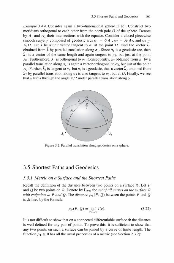
3.5 Shortest Paths and Geodesics 161
Example 3.4.4. Consider again a two-dimensional sphere in R3. Construct twomeridians orthogonal to each other from the north pole O of the sphere. Denoteby A1 and A2 their intersections with the equator. Consider a closed piecewisesmooth curve γ composed of geodesic arcs σ1 = O A1, σ2 = A1 A2, and σ3 =A2 O . Let �λ be a unit vector tangent to σ1 at the point O . Find the vector �λ1
obtained from �λ by parallel translation along σ1. Since σ1 is a geodesic arc, then�λ1 is a vector of the same length and again tangent to σ1, but just at the pointA1. Furthermore, �λ1 is orthogonal to σ2. Consequently, �λ2 obtained from �λ1 by aparallel translation along σ2 is again a vector orthogonal to σ2, but just at the pointA2. Further, �λ1 is tangent to σ3, but σ3 is a geodesic, thus a vector �λ3 obtained from�λ2 by parallel translation along σ3 is also tangent to σ3, but at O . Finally, we seethat �λ turns through the angle π/2 under parallel translation along γ .
Figure 3.2. Parallel translation along geodesics on a sphere.
3.5 Shortest Paths and Geodesics
3.5.1 Metric on a Surface and the Shortest Paths
Recall the definition of the distance between two points on a surface �. Let Pand Q be two points on �. Denote by LP Q the set of all curves on the surface �
with endpoints at P and Q. The distance ρ�(P, Q) between the points P and Qis defined by the formula
ρ�(P, Q) = infc∈LP Q
l(c). (3.22)
It is not difficult to show that on a connected differentiable surface � the distanceis well-defined for any pair of points. To prove this, it is sufficient to show thatany two points on such a surface can be joined by a curve of finite length. Thefunction ρ� ≥ 0 has all the usual properties of a metric (see Section 2.3.2):

162 3. Intrinsic Geometry of Surfaces
(1) ρ�(P, Q) = ρ�(Q, P),
(2) ρ�(P, Q) + ρ�(Q, R) ≥ ρ�(P, R),
(3) ρ�(P, Q) = 0 ⇐⇒ P = Q.
(3.23)
Further, in the cases in which it would not lead to a contradiction, the distanceρ�(P, Q) between the points P and Q is denoted by P Q.
Definition 3.5.1. The shortest path joining two points P and Q is a curve, whoselength is P Q.
3.5.2 Stationary Curves of the Length Functional
Let γ be a twice continuously differentiable curve on � located in some coordi-nate neighborhood U ; ui = ui (t) (i = 1, 2) its equations, t a canonical parame-ter, a ≤ t ≤ b. Find necessary conditions for γ to be a shortest path. Consider thecurve γε(t) given by the equations{
u1 = u1(t) + εη1(t) = u1(t, ε),
u2 = u2(t) + εη2(t) = u2(t, ε),(3.24)
and require that the curve γε(t) have the same endpoints as a curve γ (t). For thisit is sufficient to assume that the following equations hold:
ηi (a) = ηi (b) = 0 (i = 1, 2). (3.25)
From (3.24) it follows that γ0 = γ . If we now fix the functions η1 and η2, thenl(ε) = l(γε), and the length of γε is a function of ε only. Thus for γ to be ashortest path, it is necessary that it satisfy⎧⎪⎨⎪⎩
dl
dε
∣∣∣ε=0
= 0
l(ε) =∫ b
aF(ui , ui ′) dt,
(3.26)
where
ui ′ = dui
dt, F(ui , ui ′) =
√gi j (ui )ui ′u j ′,
dl
dε
∣∣∣ε=0
=∫ b
a
(∂ F
∂ uiηi + ∂ F
∂ ui ′ ηi ′)
dt = ∂ F
∂ uiηi∣∣∣ba−∫ b
a
(∂ F
∂ ui− d
dt
∂ F
∂ ui ′
)ηi dt.
The nonintegral term is zero in view of the conditions (3.25). Thus from (3.26)we obtain ∫ b
a
(∂ F
∂ui− d
dt
∂ F
∂ui ′
)ηi dt = 0. (3.27)

3.5 Shortest Paths and Geodesics 163
Recall now that η1(t) and η1(t) are arbitrary functions satisfying the conditions(3.25) only. Set
f 1 = ∂ F
∂u1− d
dt
∂ F
∂u1′ , f 2 = ∂ F
∂u2− d
dt
∂ F
∂u2′ ,
and assume that
η1 = f 1 sin2 π(t − a)
b − a, η2 = f 2 sin2 π(t − a)
b − a.
Substituting η1(t) and η2(t) into (3.27), we obtain∫ b
a
[( f 1)2 + ( f 2)2
]sin2 π(t − a)
b − adt = 0,
from which follows f 1 = f 2 = 0, or
d
dt
∂ F
∂ui− ∂ F
∂ui ′ = 0 (i = 1, 2). (3.28)
The system of equations (3.28) is called an Euler system, and the curves thatare the solutions of this system are called the stationary curves of the lengthfunctional. Writing down the equations (3.28) for the length functional F =√
gi j ui ′u j ′, we have
∂ F
∂ui ′ = gpi u p′√gi j ui ′u j ′ = 1
Cgpi u
p′,
and because t is a canonical parameter, we have√
gi j ui ′u j ′ = C . Therefore,
d
dt
(∂ F
∂ui ′
)= 1
C
(∂gpk
∂ui
du p
dt
duk
dt+ gpi
d2u p
dt2
).
Moreover,
∂ F
∂ui= 1
2√
gi j ui ′u j ′
(∂gpk
∂ui
du p
dt
duk
dt
)= 1
2C
(∂gpk
∂ui
du p
dt
duk
dt
).
Substituting the expressions for ∂ F∂ui and d
dt
(∂ F∂ui ′
)in (3.28), we obtain
gipd2u p
dt2+ ∂gpi
∂uk
duk
dt
du p
dt− 1
2
∂gpk
∂ui
du p
dt
duk
dt= 0. (3.29)
Note that∂gpi
∂uk
duk
dt
du p
dt= 1
2
(∂gpi
∂uk+ ∂gki
∂u p
)du p
dt
duk
dt.
Therefore, (3.29) can be rewritten in the following form:
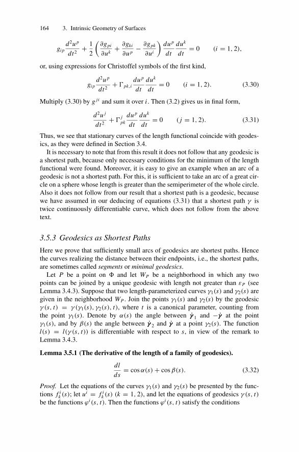
164 3. Intrinsic Geometry of Surfaces
gipd2u p
dt2+ 1
2
(∂gpi
∂uk+ ∂gki
∂u p− ∂gpk
∂ui
)du p
dt
duk
dt= 0 (i = 1, 2),
or, using expressions for Christoffel symbols of the first kind,
gipd2u p
dt2+ �pk,i
du p
dt
duk
dt= 0 (i = 1, 2). (3.30)
Multiply (3.30) by g ji and sum it over i . Then (3.2) gives us in final form,
d2u j
dt2+ �
jpk
du p
dt
duk
dt= 0 ( j = 1, 2). (3.31)
Thus, we see that stationary curves of the length functional coincide with geodes-ics, as they were defined in Section 3.4.
It is necessary to note that from this result it does not follow that any geodesic isa shortest path, because only necessary conditions for the minimum of the lengthfunctional were found. Moreover, it is easy to give an example when an arc of ageodesic is not a shortest path. For this, it is sufficient to take an arc of a great cir-cle on a sphere whose length is greater than the semiperimeter of the whole circle.Also it does not follow from our result that a shortest path is a geodesic, becausewe have assumed in our deducing of equations (3.31) that a shortest path γ istwice continuously differentiable curve, which does not follow from the abovetext.
3.5.3 Geodesics as Shortest Paths
Here we prove that sufficiently small arcs of geodesics are shortest paths. Hencethe curves realizing the distance between their endpoints, i.e., the shortest paths,are sometimes called segments or minimal geodesics.
Let P be a point on � and let WP be a neighborhood in which any twopoints can be joined by a unique geodesic with length not greater than εP (seeLemma 3.4.3). Suppose that two length-parameterized curves γ1(s) and γ2(s) aregiven in the neighborhood WP . Join the points γ1(s) and γ2(s) by the geodesicγ (s, t) = γ (γ1(s), γ2(s), t), where t is a canonical parameter, counting fromthe point γ1(s). Denote by α(s) the angle between γ 1 and −γ at the pointγ1(s), and by β(s) the angle between γ 2 and γ at a point γ2(s). The functionl(s) = l(γ (s, t)) is differentiable with respect to s, in view of the remark toLemma 3.4.3.
Lemma 3.5.1 (The derivative of the length of a family of geodesics).
dl
ds= cos α(s) + cos β(s). (3.32)
Proof. Let the equations of the curves γ1(s) and γ2(s) be presented by the func-tions f i
k (s); let ui = f ik (s) (k = 1, 2), and let the equations of geodesics γ (s, t)
be the functions ϕi (s, t). Then the functions ϕi (s, t) satisfy the conditions
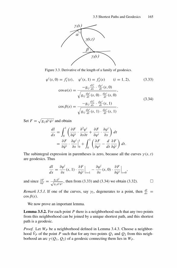
3.5 Shortest Paths and Geodesics 165
Figure 3.3. Derivative of the length of a family of geodesics.
ϕi (s, 0) = f i1 (s), ϕi (s, 1) = f i
2 (s) (i = 1, 2), (3.33)
cos α(s) = −gi jd f i
1ds · dϕ j
dt (s, 0)√gi j
dϕi
dt (s, 0) · dϕ j
dt (s, 0)
,
cos β(s) = −gi jd f i
2ds · dϕ j
dt (s, 1)√gi j
dϕi
dt (s, 1) · dϕ j
dt (s, 1)
.
(3.34)
Set F = √gi j ϕi ϕ j and obtain
dl
ds=∫ 1
0
(∂ F
∂ϕi· ∂2ϕi
∂s∂t+ ∂ F
∂ϕi· ∂ϕi
∂s
)dt
= ∂ F
∂ϕi· ∂ϕi
∂s
∣∣∣10+∫ 1
0
(∂ F
∂ϕi− d
dt
∂ F
∂ϕi
)dt.
The subintegral expression in parentheses is zero, because all the curves γ (s, t)are geodesics. Thus
dl
ds= ∂ϕi
∂s(s, 1) · ∂ F
∂ϕi
∣∣∣t=1
− ∂ϕi
∂s(s, 0) · ∂ F
∂ϕi
∣∣∣t=0
,
and since ∂ F∂ϕi = gi j ϕ
i√gi j ϕi ϕ j
, then from (3.33) and (3.34) we obtain (3.32). �
Remark 3.5.1. If one of the curves, say γ1, degenerates to a point, then dlds =
cos β(s).
We now prove an important lemma.
Lemma 3.5.2. For each point P there is a neighborhood such that any two pointsfrom this neighborhood can be joined by a unique shortest path, and this shortestpath is a geodesic.
Proof. Let WP be a neighborhood defined in Lemma 3.4.3. Choose a neighbor-hood VP of the point P such that for any two points Q1 and Q2 from this neigh-borhood an arc γ (Q1, Q2) of a geodesic connecting them lies in WP .
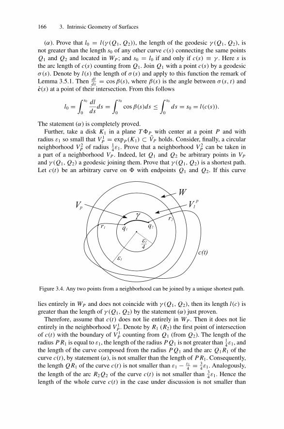
166 3. Intrinsic Geometry of Surfaces
(α). Prove that l0 = l(γ (Q1, Q2)), the length of the geodesic γ (Q1, Q2), isnot greater than the length s0 of any other curve c(s) connecting the same pointsQ1 and Q2 and located in WP ; and s0 = l0 if and only if c(s) ≡ γ . Here s isthe arc length of c(s) counting from Q1. Join Q1 with a point c(s) by a geodesicσ(s). Denote by l(s) the length of σ(s) and apply to this function the remark ofLemma 3.5.1. Then dl
ds = cos β(s), where β(s) is the angle between σ(s, t) andc(s) at a point of their intersection. From this follows
l0 =∫ s0
0
dl
dsds =
∫ s0
0cos β(s)ds ≤
∫ s0
0ds = s0 = l(c(s)).
The statement (α) is completely proved.Further, take a disk K1 in a plane T �P with center at a point P and with
radius ε1 so small that V 1P = expP(K1) ⊂ VP holds. Consider, finally, a circular
neighborhood V 2P of radius 1
4ε1. Prove that a neighborhood V 2P can be taken in
a part of a neighborhood VP . Indeed, let Q1 and Q2 be arbitrary points in VP
and γ (Q1, Q2) a geodesic joining them. Prove that γ (Q1, Q2) is a shortest path.Let c(t) be an arbitrary curve on � with endpoints Q1 and Q2. If this curve
Figure 3.4. Any two points from a neighborhood can be joined by a unique shortest path.
lies entirely in WP and does not coincide with γ (Q1, Q2), then its length l(c) isgreater than the length of γ (Q1, Q2) by the statement (α) just proven.
Therefore, assume that c(t) does not lie entirely in WP . Then it does not lieentirely in the neighborhood V 1
P . Denote by R1 (R2) the first point of intersectionof c(t) with the boundary of V 1
P counting from Q1 (from Q2). The length of theradius P R1 is equal to ε1, the length of the radius P Q1 is not greater than 1
4ε1, andthe length of the curve composed from the radius P Q1 and the arc Q1 R1 of thecurve c(t), by statement (α), is not smaller than the length of P R1. Consequently,the length Q R1 of the curve c(t) is not smaller than ε1 − ε1
4 = 34ε1. Analogously,
the length of the arc R2 Q2 of the curve c(t) is not smaller than 34ε1. Hence the
length of the whole curve c(t) in the case under discussion is not smaller than

3.5 Shortest Paths and Geodesics 167
32ε1. On the other hand, the length of the geodesic γ (Q1, Q2), again in view ofstatement (α), is not greater than the sum of the lengths of radii P Q1 and P Q2,which is equal to 1
2ε1. Comparing these two results, we obtain the statement ofthe lemma. �
A neighborhood where the statements of Lemma 3.5.2 hold is called canonical.
Problem 3.5.1. Prove that the neighborhoods mentioned in Example 3.4.2 andProblem 3.4.3 are canonical neighborhoods.
From Lemma 3.5.2 we can deduce some important theorems.
Theorem 3.5.1. For each inner point P on a geodesic γ there is an arc Q R suchthat P ∈ Q R and the arc Q R is a shortest path.
Proof. Let VP be a canonical neighborhood of a point P . Since P is an inner pointof γ , then there exist two points Q and R on the geodesic such that P belongs tothe arc Q R and both points lie inside of VP . Then by Lemma 3.5.2, the arc Q R isa shortest path. �
The statement of Theorem 3.5.1 can also be reformulated in the following form:any sufficiently small arc of a geodesic is a shortest path.
Indeed, sufficiently large arcs of geodesics can also be shortest paths. For ex-ample, any arc of a geodesic with length not greater than π R on a sphere of radiusR and on a circular cylinder of radius R is a shortest path.
The following theorem about convex surfaces was formulated by A.D. Alek-sandrov and proved by A.V. Pogorelov [Pog].
Theorem 3.5.2. On a convex surface whose Gaussian curvature is not greaterthan k0, any arc of a geodesic of length not greater than π/
√k0 is a shortest path.
Theorem 3.5.3. Any shortest path is a geodesic.
Proof. Let VP be a canonical neighborhood of an arbitrary point P located onsome shortest path γ . Take two arbitrary points Q1 ∈ γ and Q2 ∈ γ in VP andjoin them by a geodesic γ (Q1, Q2). By Lemma 3.5.2, this geodesic is the uniqueshortest path joining Q1 and Q2. Consequently, γ (Q1, Q2) ⊂ γ . Since Q1, Q2
were chosen arbitrarily, then our theorem is completely proved. �Theorem 3.5.4. For each compact set F there is a real d > 0 such that any twopoints from F whose mutual distance is smaller than d, can be joined by a uniqueshortest path.13
Proof. Let {VP} be a system of canonical neighborhoods that are constructed forall P ∈ F . This system covers the whole of F . Since F is a compact set, onecan select a finite cover V1 = VP1 , . . . , Vn = VPn . Consider a real d (Lebesguenumber) so small that any two points whose mutual distance is smaller than dbelong to one of the above neighborhoods {Vi }1≤i≤n . Then the statement of thetheorem follows from Lemma 3.5.2. �
13 d is an elementary length of the compact set F .

168 3. Intrinsic Geometry of Surfaces
Theorem 3.5.5. If two different shortest paths γ1 and γ2 have two common pointsP1 and P2, then these points are the ends of γ1, and so of γ2.
Proof. Assume the contrary. Let, for instance, P2 be an inner point of γ2. Denote
by P1 P2 the arc of a shortest path γ1, and by P1 P2 the arc of a shortest path γ2.Take a point Q1 ∈ P1 P2, Q1 �= P2, in a canonical neighborhood VP2 of P2 and a
point Q2 �= P2, Q2 ∈ γ2, Q2 /∈ P1 P2. By the triangle inequality we have
Q1 Q2 ≤ Q1 P2 + P2 Q2. (3.35)
But by Lemma 3.5.2, the equality in (3.35) is possible if and only if the arc Q1 P2
lies on γ2, and from this it would follow by Theorem 3.5.3 that the shortest pathsγ1 and γ2 coincide. Hence
Q1 Q2 < Q1 P2 + P2 Q2. (3.36)
Now consider a shortest path P1 Q2, an arc of a shortest path γ2. From the defini-tion of shortest path and (3.36) it follows that
Q1 Q2 = P1 P2 + P2 Q2 = l(P1 P2) + P2 Q2
= P1 Q1 + Q1 P2 + P2 Q2 > P1 Q1 + Q1 Q2,
which contradicts the triangle inequality. �
3.5.4 Complete Surfaces
Definition 3.5.2. A surface � is geodesically complete if each its geodesic seg-ments can be extended limitlessly.
Theorem 3.5.6 (Hopf–Rinow). If a surface � is geodesically complete, then anytwo of its points can be joined by a shortest path.
Proof (see [Miln] ). Let P and Q be points on �, P �= Q, P Q = a. Take a circle�δ in a canonical neighborhood VP of a point P with radius δ. Since the set �δ
is compact, there is a point Pδ on �δ for which Pδ Q is equal to the distance fromQ to the set �δ . Draw a geodesic γ (t) through the points P and Q, where t isan arc length parameter counting from P . Prove that γ (a) = Q and that an arcof γ (t) for 0 ≤ t ≤ a is a shortest path joining P and Q. Since any curve withendpoints P and Q intersects �δ , then by definition of the distance and in view ofLemma 3.5.2, the following equality is true:
δ + Pδ Q = P Q = a. (3.37)
Let F be the set of real t ∈ (0, a] satisfying the equality
t + γ (t)Q = P Q. (3.38)

3.5 Shortest Paths and Geodesics 169
The set F is nonempty, as is seen from (3.37); it is closed in view of continuityof metrical function ρ�; and it is connected in view of the triangle inequality.Suppose that t0 = supt∈F t . If t0 = a, then the theorem is proved.
Thus we suppose that t0 < a, and this will lead to a contradiction. Take a circle�1 of radius δ1 in a canonical neighborhood Vγ (t0) = V0 of the point γ (t0), andselect δ1 such that δ1 < min(t0, a − t0) holds. Take a point Pδ1 = P1 on �1 suchthat
δ1 + P1 Q = γ (t0)Q. (3.39)
The existence of the above point P1 can be proved similarly to how the existenceof Pδ was proved. Now two cases are possible:
(1) P1 ∈ γ, (2) P1 /∈ γ.
In the first case, from (3.38) and (3.39) it follows that t0 + δ1 ∈ F , contrary tothe definition of t0. So, one needs to study only the second case. In this case, by
Figure 3.5. Geodesically complete surface.
Lemma 3.5.2,
γ (t0 − δ)P1 < 2δ, (3.40)
and from (3.38)–(3.40) follows
P Q ≤ Q P1 + P1γ (t0 − δ1) + γ (t0 − δ1)P
< Q P1 + 2δ1 + t0 − δ1 = t0 + δ1 + γ (t0)Q = P Q,
i.e., P Q < P Q. This contradiction implies that t0 = a, and the theorem isproved. �Remark 3.5.2. The assumption of geodesic completeness in Theorem 3.5.6 is nec-essary. Indeed, if we delete at least one point O from the Euclidean plane R2, thenthe points P1 and P2, which lie on a same straight line with O , cannot be joinedby a shortest path if O is located between P1 and P2. In addition to the geodesiccompleteness of a surface one can also define metrical completeness, i.e., com-pleteness with respect to the metrical function ρ�(P, Q). It turns out that boththese notions of completeness are equivalent.

170 3. Intrinsic Geometry of Surfaces
Theorem 3.5.7. A surface � is geodesically complete if and only if it is metricallycomplete.
Proof. Assume that � is metrically complete. Then the property of geodesic com-pleteness follows from well-known theorems of the theory of ordinary differentialequations. Conversely, let � be a geodesically complete surface. Take a boundedand closed set F on � in the sense of the metric ρ�(P, Q). We prove that F iscompact. Denote by d the diameter of F . Let Q ∈ F . Construct a closed disk Kof radius d in the plane T �Q . Since � is geodesically complete, expQ is definedon the whole of K . The set expQ K , as the continuous image of a compact set,is also a compact set. In view of Theorem 3.5.6, the set F belongs to expQ K ;consequently, it is also compact. �
Note that from Theorems 3.5.6 and 3.5.7 it follows that for any point Q on acomplete surface � the mapping expQ is defined on the whole plane T �Q andmaps it onto all of �.
3.5.5 Convex Regions on a Complete Surface
Consider the form taken by the well-known notion of a convex region in Euclideangeometry. Let D be some closed region. For simplicity, assume it to be homeo-morphic to a disk. Define the distance between points P and Q of a region D withrespect to D by the rule
ρD(P, Q) = infc∈LP Q(D)
l(c), (3.41)
where LP Q(D) is the set of all curves in D joining P with Q. A curve joiningP and Q whose length is ρD(P, Q) is called a shortest path in the region D.A region D on a surface � is geodesically convex if any shortest path in D is ageodesic on �. It turns out that geodesically convex regions, similarly to convexregions in the Euclidean plane R2, can be characterized locally.
Theorem 3.5.8. A region D is geodesically convex if and only if the geodesiccurvature of its boundary at each point is nonnegative (in the direction of D).
We leave it to reader as an exercise to find a proof of this theorem.
Definition 3.5.3. A region D on a surface is called convex if each shortest path inD is at the same time a shortest path on �.
Theorem 3.5.9. Find an example of a surface and a region on it that is geodesi-cally convex, but not convex.
Definition 3.5.4. A region D on a surface � is called totally convex if any shortestpath on � with ends in D lies entirely in D.
Problem 3.5.2. Find an example of a surface and a region on it that is convex butnot totally convex.
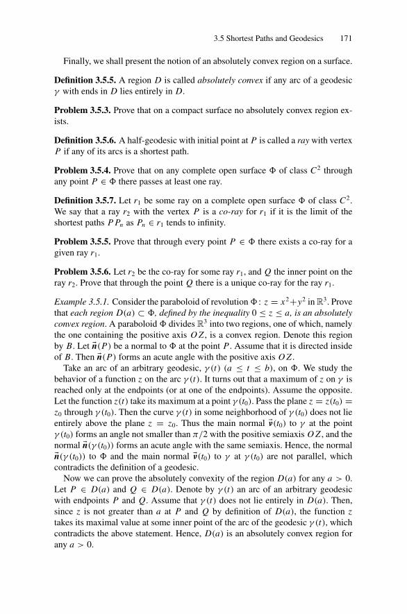
3.5 Shortest Paths and Geodesics 171
Finally, we shall present the notion of an absolutely convex region on a surface.
Definition 3.5.5. A region D is called absolutely convex if any arc of a geodesicγ with ends in D lies entirely in D.
Problem 3.5.3. Prove that on a compact surface no absolutely convex region ex-ists.
Definition 3.5.6. A half-geodesic with initial point at P is called a ray with vertexP if any of its arcs is a shortest path.
Problem 3.5.4. Prove that on any complete open surface � of class C2 throughany point P ∈ � there passes at least one ray.
Definition 3.5.7. Let r1 be some ray on a complete open surface � of class C2.We say that a ray r2 with the vertex P is a co-ray for r1 if it is the limit of theshortest paths P Pn as Pn ∈ r1 tends to infinity.
Problem 3.5.5. Prove that through every point P ∈ � there exists a co-ray for agiven ray r1.
Problem 3.5.6. Let r2 be the co-ray for some ray r1, and Q the inner point on theray r2. Prove that through the point Q there is a unique co-ray for the ray r1.
Example 3.5.1. Consider the paraboloid of revolution � : z = x2+y2 in R3. Provethat each region D(a) ⊂ �, defined by the inequality 0 ≤ z ≤ a, is an absolutelyconvex region. A paraboloid � divides R3 into two regions, one of which, namelythe one containing the positive axis O Z , is a convex region. Denote this regionby B. Let �n(P) be a normal to � at the point P . Assume that it is directed insideof B. Then �n(P) forms an acute angle with the positive axis O Z .
Take an arc of an arbitrary geodesic, γ (t) (a ≤ t ≤ b), on �. We study thebehavior of a function z on the arc γ (t). It turns out that a maximum of z on γ isreached only at the endpoints (or at one of the endpoints). Assume the opposite.Let the function z(t) take its maximum at a point γ (t0). Pass the plane z = z(t0) =z0 through γ (t0). Then the curve γ (t) in some neighborhood of γ (t0) does not lieentirely above the plane z = z0. Thus the main normal �ν(t0) to γ at the pointγ (t0) forms an angle not smaller than π/2 with the positive semiaxis O Z , and thenormal �n(γ (t0)) forms an acute angle with the same semiaxis. Hence, the normal�n(γ (t0)) to � and the main normal �ν(t0) to γ at γ (t0) are not parallel, whichcontradicts the definition of a geodesic.
Now we can prove the absolutely convexity of the region D(a) for any a > 0.Let P ∈ D(a) and Q ∈ D(a). Denote by γ (t) an arc of an arbitrary geodesicwith endpoints P and Q. Assume that γ (t) does not lie entirely in D(a). Then,since z is not greater than a at P and Q by definition of D(a), the function ztakes its maximal value at some inner point of the arc of the geodesic γ (t), whichcontradicts the above statement. Hence, D(a) is an absolutely convex region forany a > 0.

172 3. Intrinsic Geometry of Surfaces
3.6 Special Coordinate Systems
3.6.1 Riemannian Normal Coordinate System
Let P be an arbitrary point on the surface �. Consider the rectangular coordinatesystem u1, u2 in the plane T �P . In view of Lemma 3.4.3, there is δ such thatthe disk B(P, δ) with center at P and radius δ is uniquely mapped onto someneighborhood W of P on � under the exponential map. Let Q1 ∈ B(P, δ) andQ = expP(
−−→P Q1). Introduce a coordinate system u1, u2 in W , letting the coordi-
nates of the point Q be equal to the coordinates of the point P . Then P has zerocoordinates, and �r1(0, 0) and �r2(0, 0) are unit and mutually orthogonal vectors.Thus
g11(0, 0) = g22(0, 0) = 1, g12(0, 0) = 0.
The equations of geodesics on � passing through P will be written in the formu1 = α1t , u2 = α2t , where t is proportional to an arc length parameter and isequal to it when (α1)2 + (α1)2 = 1. Substituting these functions in the equationsof geodesics, we obtain
�ijk(α
1t, α2t)α jαk = 0 (i = 1, 2). (3.42)
Multiplying (3.42) by gip and summing over i , we obtain
� jk,p(α1t, α2t)α jαk = 0 (p = 1, 2). (3.43)
Let t = 0. Then
� jk,p(0, 0)α jαk = 0 (p = 1, 2). (3.44)
From (3.44), in view of the arbitrariness of the real α1 and α2, we have
�i j,k = 0 (i, j, k = 1, 2). (3.45)
For calculating the second derivatives of the metric tensor components, differen-tiate (3.43) with respect to t and assume that t = 0. Then
∂� jk,p
∂uiαiα jαk = 0 (p = 1, 2). (3.46)
Write down (3.46) in detail:
(α1)3 ∂�11,p
∂u1+ (α1)2α2
(∂�11,p
∂u2+ ∂�12,p
∂u1
)+ α1(α2)2
(∂�22,p
∂u1+ ∂�12,p
∂u2
)+ (α2)3 ∂�22,p
∂u2= 0 (p = 1, 2). (3.47)
From (3.47) we obtain eight equations:

3.6 Special Coordinate Systems 173
∂�11,p
∂u1(0, 0) = ∂2g1p
(∂u1)2− 1
2
∂2g11
∂u1∂u p= 0 (p = 1, 2), (3.48)
∂�11,p
∂u2(0, 0) + 2
∂�12,p
∂u1(0, 0) = ∂2g1p
∂u1∂u2− 1
2
∂2g11
∂u2∂u p
+ ∂2g1p
∂u1∂u2+ ∂2g2p
(∂u1)2− ∂2g12
∂u1∂u p= 0 (p = 1, 2), (3.49)
∂�22,p
∂u1(0, 0) + 2
∂�12,p
∂u2(0, 0) = ∂2g2p
∂u1∂u2− 1
2
∂2g22
∂u1∂u p
+ ∂2g1p
(∂u2)2+ ∂2g2p
∂u1∂u2− ∂2g12
∂u2∂u p= 0 (p = 1, 2), (3.50)
∂�22,p
∂u2(0, 0) = ∂2g2p
(∂u2)2− 1
2
∂2g22
∂u2∂u p= 0 (p = 1, 2). (3.51)
We add to these equations the expression for the Gaussian curvature K of a surface� at P . In view of (3.45), we obtain
K = 1
2
(2
∂2g12
∂u1∂u2− ∂2g11
(∂u2)2− ∂2g22
(∂u1)2
). (3.52)
Solving the system (3.48)–(3.52), we obtain
∂2g11
(∂u1)2(0, 0) = ∂2g11
∂u1∂u2(0, 0) = ∂2g12
(∂u1)2(0, 0)
= ∂2g22
∂u1∂u2(0, 0) = ∂2g12
(∂u2)2(0, 0) = 0,
∂2g11
(∂u2)2(0, 0) = ∂2g22
(∂u1)2(0, 0) = −2
3K (0, 0),
∂2g12
∂u1∂u2(0, 0) = 1
3K (0, 0). (3.53)
From (3.53) it follows that
g11 = 1 − 1
3K (0, 0)(u2)2 + o((u1)2 + (u2)2),
g12 = 1
3K (0, 0)u1u2 + o((u1)2 + (u2)2), (3.54)
g22 = 1 − 1
3K (0, 0)(u1)2 + o((u1)2 + (u2)2).
The formulas (3.54) give us the possibility to compare the length of an arbitrarycurve γ1 on a tangent plane T �P with the length of its image γ under the expo-nential map.
3.6.2 Comparison Theorem for Metrics
Let a curve γ1 lie inside a disk B(P, δ) in a plane T �P , and let γ be its imageunder the exponential map. Denote by l1 the length of γ1, and by l the length of γ .

174 3. Intrinsic Geometry of Surfaces
Theorem 3.6.1. There exists δ1 such that for all δ < δ0 the inequality |l − l1| ≤Cl1δ
2 holds, where the constant C does not depend on the value of the Gaussiancurvature at a point P.
Proof. Let the equations of the curve γ1 in Cartesian rectangular coordinates onT �P be presented by the functions f1(t) and f2(t); u1 = f1(t), u2 = f2(t).Then the equations of the curve γ in Riemannian normal coordinates are givenby the same functions. Let t be the arc length of the curve γ1 counting from itsinitial point. Then
[ f ′1(t)]2 + [ f ′
2(t)]2 = 1. (3.55)
Calculate the length l of the curve γ :
l =∫ l1
0
√( f ′
1)2 + ( f ′
2)2 + 1
3 K (0, 0)[2 f1 f2 f ′1 f ′
2 − f 21 ( f ′
1)2 − f 2
2 ( f ′2)
2] + o(δ2) dt.
(3.56)
Set
A = 1
3K (0, 0)(2 f1 f2 f ′
1 f ′2 − f 2
1 ( f ′1)
2 − f 22 ( f ′
2)2) + o(δ2).
Then
|l − l1| =∫ l1
0(√
1 + A − 1) dt =∫ l1
0
A dt√1 + A + 1
.
We estimate |A| from above:
|A| ≤ 1
3|K (0, 0)| · 2[ f 2
1 ( f ′1)
2 + f 22 ( f ′
2)2] + o(δ2).
Since | f ′1| ≤ 1 and | f ′
2| ≤ 1, for a sufficiently small δ we obtain
|A| ≤ 1
3|K (0, 0)|2δ2 + o(δ2) ≤ |K (0, 0)|δ2.
We estimate√
1 + A + 1 from below. In view of the previous inequality, we have√1 + A + 1 > 3
2 . We thus obtain
|l − l1| ≤ 2
3|K (0, 0)|δ2
∫ l1
0dt = 2
3|K (0, 0)|l1δ
2. �
In particular, let γ1 be the circle of radius δ with center at P in the plane T �P ,and γ the circle of radius δ with center at P on �. Then from Theorem 3.6.1follows l = 2πδ + o(δ2), and if γ is an arc of a circle with a central angle α, then
l = αδ + o(δ2). (3.57)
Corollary 3.6.1. Let A ∈ B(P, δ), B ∈ B(P, δ), A = exp−1P (A), and B =
exp−1P (B). Then AB = A B + o(δ).
Proof. Let γ = expP( A B), and γ = exp−1P (AB). Then, in view of Theo-
rem 3.6.1, we have l = l(γ ) = A B + o(δ), l = l(γ ) = AB + o(δ). But sinceAB ≤ l, A B < l, then AB ≤ A B + o(δ), A B ≤ AB + o(δ). From the two lastinequalities it follows that AB = A B + o(δ). �
3.6 Special Coordinate Systems 175
3.6.3 Geodesic Polar Coordinates on a Surface
Let P be an arbitrary point on a surface �. Introduce a polar coordinate sys-tem with the center at a point P in the plane T �P . In view of Lemma 3.4.3,there is δ0 > 0 such that for all δ (0 < δ < δ0) the exponential map expP isa diffeomorphism of a disk B(P, δ) ⊂ T �P onto some neighborhood W ⊂ �.Introduce coordinates (ρ, ϕ) in W , assuming coordinates of a point Q equal tothe coordinates of its inverse image under the exponential map expP . This coordi-nate system is called a geodesic polar coordinate system with the origin at P , anda neighborhood W itself is called a disk, which we denote by the same symbolB(P, δ). The point P is a singular point of this coordinate system: |�rρ(0, 0)| = 1,and |�rϕ(0, 0)| = 0. Therefore,
g11(0, 0) = 〈�rρ, �rρ〉 = 1, g22(0, 0) = 〈�rϕ, �rϕ〉 = 0,
g12(0, 0) = 〈�rρ, �rϕ〉 = 0. (3.58)
In view of Lemma 3.5.1 about the derivative of the length of a family of geodesics,we see that the coordinate curves ρ = const and ϕ = const are orthogonal. Thus
g12(ρ, ϕ) = 0. (3.59)
Set f = √g22(ρ, ϕ). Then from (3.58) it follows that
f (0, ϕ) = 0. (3.60)
We prove that f ′ρ(0, ϕ) = 1. Let l(ρ, α) be an arc length parameter of the circle
of radius ρ and center at P and with central angle α on �. Then
l(ρ, α) =∫ α
0
√g22(ρ, ϕ) dϕ.
Hence from (3.57) follows the identity∫ α
0
√g22(ρ, ϕ) dϕ = αρ + o(ρ).
Differentiating the last equality with respect to ρ and α, assuming then ρ = 0, weget
d
dρ
(g22(ρ, ϕ)
)∣∣ρ=0 = 1,
or
f ′ρ(0, ϕ) = 1. (3.61)
We now calculate the Gaussian curvature K of the surface �. In view of equalities(3.58) and (3.59), we obtain
K (ρ, ϕ) = − f ′′ρρ(ρ, ϕ)/ f (ρ, ϕ). (3.62)
176 3. Intrinsic Geometry of Surfaces
We rewrite (3.62) in the following form:
f ′′ρρ(ρ, ϕ) + K (ρ, ϕ) f (ρ, ϕ) = 0, (3.63a)
f (0, ϕ) = 0, f ′ρ(0, ϕ) = 1. (3.63b)
Equation (3.63a) and initial conditions (3.63b) show us that if K (ρ, ϕ) is a knownfunction of coordinates (ρ, ϕ), then g22(ρ, ϕ) is uniquely defined and all coeffi-cients of the metric tensor can be obtained. For instance, let K (ρ, ϕ) = ±a2.
Then g11 = 1, g12 = 0, g22 = 1a2 sin2(aρ) or g22 = 1
a2 sinh2(aρ) in the case ofK = −a2.
3.6.4 Semigeodesic Coordinate System on a Surface
Take on a surface � a closed arc of a geodesic γ without points of self-intersection.Introduce on γ an arc length parameterization γ (t) (0 ≤ t ≤ b), counting fromsome point. Pass a geodesic σ(t, s) through every point γ (t) orthogonal to γ ,where s is an arc length parameter on σ(t, s), starting from the point γ (t). Provethat there is δ0 > 0 such that for |s| < δ0 none of the geodesics σ(t, s) inter-sect for a sufficiently small extension. First, prove that two sufficiently nearbygeodesics σ(t, s) do not intersect on a sufficiently small extension.
Take some point γ (t), and let any coordinates u1, u2 be defined in its neighbor-hood. Let γ (t) have the equations ui = ui (t) (i = 1, 2), and let σ(t, s) have theequations ui = hi (t, s). Then
hi (t, s) = ui (t) (i = 1, 2). (3.64)
Prove that the determinant � =∣∣∣ ∂h1
∂t∂h2
∂t∂h1
∂s∂h2
∂s
∣∣∣ is nonzero for s = 0. Set λi = ∂hi
∂t
∣∣s=0
and µi = ∂hi
∂s
∣∣s=0. Then λi are coordinates of a unit vector �λ that is tangent to
γ (t) at the point γ (t), and µi are coordinates of a unit vector �µ that is tangentto the geodesic σ(t, s) at the point σ(t, 0) = γ (t). Since �λ and �µ are mutuallyorthogonal vectors by their construction, then � �= 0. From this and the implicitfunction theorem it follows that for each t1 there exist real numbers δ(t1) and ε(t1)such that for t1 − ε(t1) < t < t1 + ε(t1) the arcs of the geodesics σ(t, s) do notintersect. Moreover, all points σ(t, s) for t1 − ε(t1) < t < t1 + ε(t1), |s| < δ(t1)form a region on �. Since the closed arc γ is compact, there exist real numbers δ1
and ε1 such that the arcs of geodesics σ(t1, s) and σ(t2, s) do not intersect when|s| < δ1 and |t2 − t1| < ε1.
Now let δ2 = min{ρ(γ (t), γ (t + t ′)) : t, t ′ ∈ [a, b], t ′ ≥ ε′}. Define δ0 =12 min{δ1, δ2}. It is not difficult to check that δ0 is the required real number. Con-sider the region on the surface � consisting of the points σ(t, s) for a ≤ t ≤ b.Introduce coordinates in this region, assuming u1 = s, u2 = t . The obtainedcoordinates are called semigeodesic coordinates.
Remark 3.6.1. In the construction of semigeodesic coordinates one can, generallyspeaking, take an arbitrary regular curve instead of a geodesic γ .

3.6 Special Coordinate Systems 177
Figure 3.6. Semigeodesic coordinates on a surface.
We now study the structure of the coefficients of the first fundamental formof a surface in a semigeodesic coordinate system. The coordinate curves u1 =const and u2 = const intersect in a right angle. This statement follows from theconstruction of the coordinate system and from Lemma 3.5.1 about the derivativeof the length of a family of geodesics. Therefore,
g21(u1, u2) = 0. (3.65)
Furthermore, since u1 is the length of the curve u2 = const, then
g11(u1, u2) = 1. (3.66)
Thus,
ds2 = (du1)2 + g22(u1, u2)(du2)2. (3.67)
Assuming f (u1, u2) = √g22, we obtain, as in Section 3.6.3
∂2 f
(∂u1)2+ K (u1, u2) f (u1, u2) = 0. (3.68)
However, the initial conditions are different. Since for u1 = 0, u2 is the length ofγ , then √
g22(0, u2) = f (0, u2) = 1. (3.69)
Finally, u1 = 0, u2 = t is a geodesic; consequently,
�122(0, u2) = �2
22(0, u2) = 0. (3.70)
Using the expressions of Christoffel symbols of the first kind, we obtain
− f (0, u2)∂ f
∂u1(0, u2) = 0,
and from this follows
178 3. Intrinsic Geometry of Surfaces
∂ f
∂u1(0, u2) = 0. (3.71)
So the function f (u1, u2) satisfies (3.68) with the initial conditions (3.69) and(3.71). We calculate Christoffel symbols of the second kind for a semigeodesiccoordinate system. We have
g22 = G(u1, u2) = f 2(u1, u2), g12 = g21 = 0, g11 = 1.
Thus
�111 = �2
11 = �112 = �1
21 = 0, �122 = �22,1 = −1
2Gu1 = − f fu1 ,
�221 = �2
12 = 2
f 2f fu1 = fu1
f, �2
22 = 1
f 2�22,2 = fu2
f.
(3.72)
Furthermore, we obtain a formula for the geodesic curvature kg of an arbitrarycurve c. Let u1 = u1(t), u2 = u2(t) be the equations of c, and t an arc lengthparameter on c, counting from some point. Then we have the equalities
|c(t)| = 1,⟨c(t),
D
dtc(t)
⟩= 0. (3.73)
If we denote by µ1 and µ2 the coordinates of the vector Ddt c(t) in a local basis,
then the system (3.73) in semigeodesic coordinates is written in the followingform: (du1
dt
)2 + G(du2
dt
)2 = 1, (3.74)
µ1 du1
dt+ Gµ2 du2
dt= 0. (3.75)
Lemma 3.6.1. The geodesic curvature kg of a curve c is expressed by the formula
kg = √G
∣∣∣∣µ1 du2
dt− µ2 du1
dt
∣∣∣∣ . (3.76)
Proof. Raise the right-hand side to the second power. In view of (3.74), (3.75),and (3.21) we obtain
G
[(µ1 du2
dt
)2 +(µ2 du1
dt
)2 − 2µ1µ2 du1
dt
du2
dt
]= G
[(µ1 du2
dt
)2 +(µ2 du1
dt
)2
− µ1
G
du1
dt
(− µ1 du1
dt
)− µ2 du2
dt
(− Gµ2 du2
dt
)]= G
[(µ1)2
G
(G(du2
dt
)2 +(du1
dt
)2)
+ (µ2)2
((du1
dt
)2 + G(du2
dt
)2)]
= (µ1)2 + G(µ2)2 =∣∣∣ D
dtc(t)
∣∣∣2 = k2g. �
3.7 Gauss–Bonnet Theorem and Comparison Theorem 179
Now substitute the expressions for u1 and u2, see (3.8), in (3.76). Then thegeodesic curvature is
kg =∣∣∣∣ f
[du2
dt
d2u1
dt2− f fu1
(du2
dt
)2]
− fdu1
dt
[d2u2
dt2+ 2
fu1
f
du1
dt
du2
dt+ fu2
f
(du2
dt
)2]∣∣∣∣ .
Simplifying the sums of the above terms yields
− f 2 fu1
(du2
dt
)3
− fu1
(du1
dt
)2du2
dt
= −du2
dtfu1
[f 2
(du2
dt
)2
+(
du1
dt
)2]
= − fu1du2
dt.
Consequently,
kg =∣∣∣∣ f(d2u1
dt2
du2
dt− d2u2
dt2
du1
dt
)− fu1
((du1
dt
)2 + 1
)du2
dt− fu2
(du2
dt
)2 du1
dt
∣∣∣∣ . (3.77)
3.7 Gauss–Bonnet Theorem and Comparison Theoremfor the Angles of a Triangle
Consider a region W on a complete surface � that is homeomorphic to a disk andthat lies in some coordinate neighborhood U with coordinates (u1, u2). Introducean orientation in W , induced by coordinates (u1, u2); i.e., define a basis �r1 = �ru1 ,�r2 = �ru2 at each point of W . Assume that the boundary of W is a curve c ofclass C2. Take a field of normals �a along c, directed inside of W . Introduce aparameterization on c such that the ordered pair of vectors {�a, c(t)} forms a basisequivalent to the basis {�r1, �r2}. Define the sign of the geodesic curvature kg of thecurve c(t) in the following way.
If the basis{
Ddt c(t), c(t)
}is equivalent to the basis {�a, c(t)}, then suppose kg >
0, and kg < 0 for the opposite case. If µ1, µ2 are the components of Ddt c(t) in this
basis {�r1, �r2}, and (c1, c2) are the components of c(t) in the same basis, then the
signs of the curvature kg and the determinant∣∣∣ µ1 µ2
c1 c2
∣∣∣ = µ1c2 −µ2c1 coincide. So,
sign kg = sign(µ1c2 − µ2c1). (3.78)
From the geometrical point of view, the definition of sign kg is equivalent to thecondition that if kg is positive at each point on c(t), then W is a geodesicallyconvex region.
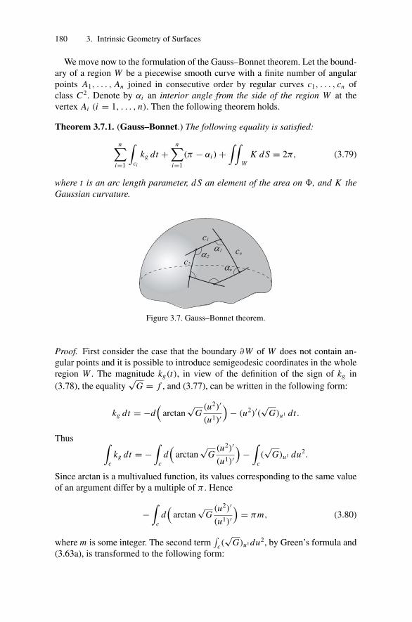
180 3. Intrinsic Geometry of Surfaces
We move now to the formulation of the Gauss–Bonnet theorem. Let the bound-ary of a region W be a piecewise smooth curve with a finite number of angularpoints A1, . . . , An joined in consecutive order by regular curves c1, . . . , cn ofclass C2. Denote by αi an interior angle from the side of the region W at thevertex Ai (i = 1, . . . , n). Then the following theorem holds.
Theorem 3.7.1. (Gauss–Bonnet.) The following equality is satisfied:
n∑i=1
∫ci
kg dt +n∑
i=1
(π − αi ) +∫∫
WK d S = 2π, (3.79)
where t is an arc length parameter, d S an element of the area on �, and K theGaussian curvature.
Figure 3.7. Gauss–Bonnet theorem.
Proof. First consider the case that the boundary ∂W of W does not contain an-gular points and it is possible to introduce semigeodesic coordinates in the wholeregion W . The magnitude kg(t), in view of the definition of the sign of kg in(3.78), the equality
√G = f , and (3.77), can be written in the following form:
kg dt = −d(
arctan√
G(u2)′
(u1)′)
− (u2)′(√
G)u1 dt.
Thus ∫c
kg dt = −∫
cd(
arctan√
G(u2)′
(u1)′)
−∫
c(√
G)u1 du2.
Since arctan is a multivalued function, its values corresponding to the same valueof an argument differ by a multiple of π . Hence
−∫
cd(
arctan√
G(u2)′
(u1)′)
= πm, (3.80)
where m is some integer. The second term∫
c(√
G)u1 du2, by Green’s formula and(3.63a), is transformed to the following form:
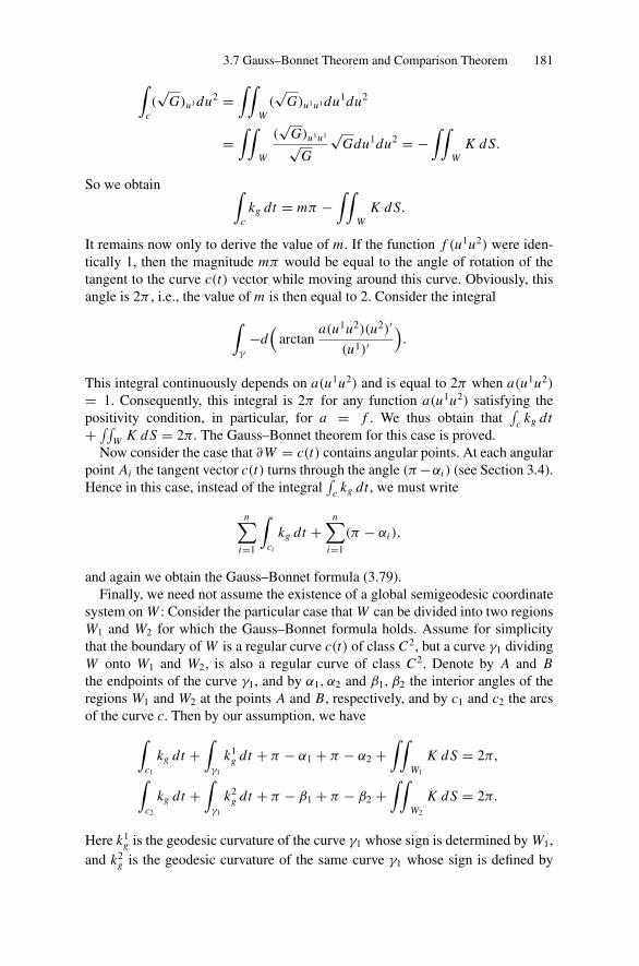
3.7 Gauss–Bonnet Theorem and Comparison Theorem 181∫c(√
G)u1 du2 =∫∫
W(√
G)u1u1 du1du2
=∫∫
W
(√
G)u1u1√G
√Gdu1du2 = −
∫∫W
K d S.
So we obtain ∫c
kg dt = mπ −∫∫
WK d S.
It remains now only to derive the value of m. If the function f (u1u2) were iden-tically 1, then the magnitude mπ would be equal to the angle of rotation of thetangent to the curve c(t) vector while moving around this curve. Obviously, thisangle is 2π , i.e., the value of m is then equal to 2. Consider the integral∫
γ
−d(
arctana(u1u2)(u2)′
(u1)′).
This integral continuously depends on a(u1u2) and is equal to 2π when a(u1u2)
= 1. Consequently, this integral is 2π for any function a(u1u2) satisfying thepositivity condition, in particular, for a = f . We thus obtain that
∫c kg dt
+ ∫∫W K d S = 2π. The Gauss–Bonnet theorem for this case is proved.
Now consider the case that ∂W = c(t) contains angular points. At each angularpoint Ai the tangent vector c(t) turns through the angle (π −αi ) (see Section 3.4).Hence in this case, instead of the integral
∫c kg dt , we must write
n∑i=1
∫ci
kg dt +n∑
i=1
(π − αi ),
and again we obtain the Gauss–Bonnet formula (3.79).Finally, we need not assume the existence of a global semigeodesic coordinate
system on W : Consider the particular case that W can be divided into two regionsW1 and W2 for which the Gauss–Bonnet formula holds. Assume for simplicitythat the boundary of W is a regular curve c(t) of class C2, but a curve γ1 dividingW onto W1 and W2, is also a regular curve of class C2. Denote by A and Bthe endpoints of the curve γ1, and by α1, α2 and β1, β2 the interior angles of theregions W1 and W2 at the points A and B, respectively, and by c1 and c2 the arcsof the curve c. Then by our assumption, we have∫
c1
kg dt +∫
γ1
k1g dt + π − α1 + π − α2 +
∫∫W1
K d S = 2π,∫c2
kg dt +∫
γ1
k2g dt + π − β1 + π − β2 +
∫∫W2
K d S = 2π.
Here k1g is the geodesic curvature of the curve γ1 whose sign is determined by W1,
and k2g is the geodesic curvature of the same curve γ1 whose sign is defined by
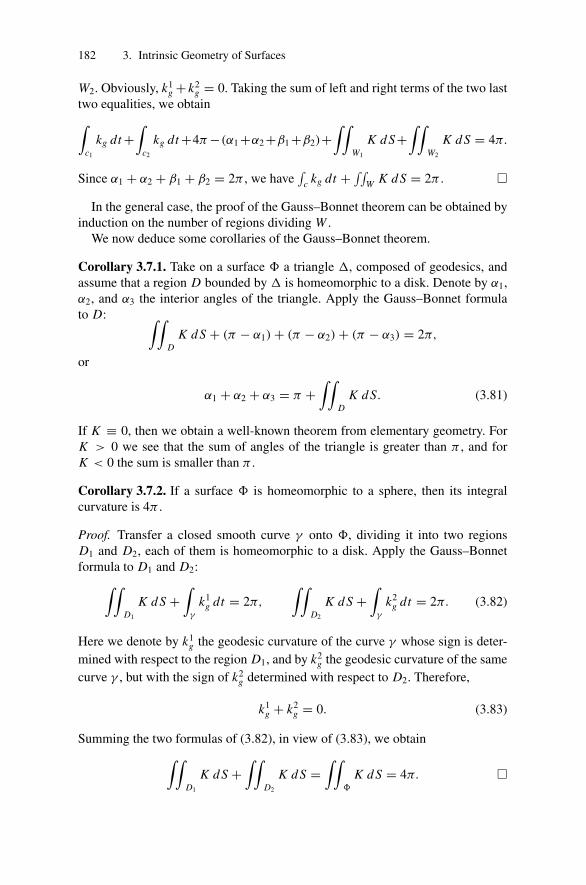
182 3. Intrinsic Geometry of Surfaces
W2. Obviously, k1g + k2
g = 0. Taking the sum of left and right terms of the two lasttwo equalities, we obtain∫
c1
kg dt +∫
c2
kg dt +4π −(α1 +α2 +β1 +β2)+∫∫
W1
K d S+∫∫
W2
K d S = 4π.
Since α1 + α2 + β1 + β2 = 2π , we have∫
c kg dt + ∫∫W K d S = 2π . �
In the general case, the proof of the Gauss–Bonnet theorem can be obtained byinduction on the number of regions dividing W .
We now deduce some corollaries of the Gauss–Bonnet theorem.
Corollary 3.7.1. Take on a surface � a triangle �, composed of geodesics, andassume that a region D bounded by � is homeomorphic to a disk. Denote by α1,α2, and α3 the interior angles of the triangle. Apply the Gauss–Bonnet formulato D: ∫∫
DK d S + (π − α1) + (π − α2) + (π − α3) = 2π,
or
α1 + α2 + α3 = π +∫∫
DK d S. (3.81)
If K ≡ 0, then we obtain a well-known theorem from elementary geometry. ForK > 0 we see that the sum of angles of the triangle is greater than π , and forK < 0 the sum is smaller than π .
Corollary 3.7.2. If a surface � is homeomorphic to a sphere, then its integralcurvature is 4π .
Proof. Transfer a closed smooth curve γ onto �, dividing it into two regionsD1 and D2, each of them is homeomorphic to a disk. Apply the Gauss–Bonnetformula to D1 and D2:∫∫
D1
K d S +∫
γ
k1g dt = 2π,
∫∫D2
K d S +∫
γ
k2g dt = 2π. (3.82)
Here we denote by k1g the geodesic curvature of the curve γ whose sign is deter-
mined with respect to the region D1, and by k2g the geodesic curvature of the same
curve γ , but with the sign of k2g determined with respect to D2. Therefore,
k1g + k2
g = 0. (3.83)
Summing the two formulas of (3.82), in view of (3.83), we obtain∫∫D1
K d S +∫∫
D2
K d S =∫∫
�
K d S = 4π. �

3.7 Gauss–Bonnet Theorem and Comparison Theorem 183
Problem 3.7.1. Prove that the integral curvature of any surface homeomorphic toa torus is 0.
Remark 3.7.1. The total Gaussian curvature of a compact surface � is∫∫�
K d S = 2πχ(�),
where χ(�) is the Euler characteristic (see Remark 2.7.1).
Problem 3.7.2 (Sine theorem for small triangles). Let �ABC be a triangle onthe regular surface of class C2, and AC = δ. Then
BC = sin α · δ/sin(α + γ ) + o(δ), AB = sin γ · δ/sin(α + γ ) + o(δ),
where α and γ are the angles of �ABC at the vertices A and C , respectively.
Solution. Introduce on AC the arc length parameterization c(s), counting fromthe point A, 0 ≤ s ≤ δ. Bring a geodesic σ(s) through the point c(s) forming anangle γ with AC , and denote by B(s) the point of intersection of σ(s) with AB.Let t (s) = AB(s), l(s) = A(s)B(s) and denote by β(s) the angle of �ABC atthe vertex B(s). Then, in view of Lemma 3.5.1, we have
dl
ds= cos γ + cos β(s)
dt
ds.
From Corollary 3.7.1 and the Gauss–Bonnet theorem follows β(s) = π − α −γ + o(s). Therefore,
dl
ds= cos γ − cos(α + γ )
dt
ds+ o(s).
Integrating the last equality with respect to s from 0 to δ, we obtain
l(δ) = BC = cos γ · δ − cos(α + γ )AB + o(δ).
Analogously, we obtain
AB = cos α · δ − cos(α + γ )BC + o(δ).
So,
BC + cos(α + γ )AB = cos γ · δ + o(δ),
BC cos(α + γ ) + AB = cos α · δ + o(δ).
From these equalities follows
AB = cos α − cos γ cos(α + γ )
sin2(α + γ )δ + o(δ) = sin γ · δ
sin(α + γ )+ o(δ),
BC = cos γ − cos α cos(α + γ )
sin2(α + γ )δ + o(δ) = sin α · δ
sin(α + γ )+ o(δ).
Finally, the formula α + β + γ = π + o(δ) follows from (3.81). �

184 3. Intrinsic Geometry of Surfaces
Consider a simply connected complete surface of nonpositive Gaussian curva-ture. Denote such a surface by �−. Recall that a surface � is simply connected ifany simple closed curve divides � into two regions, one of which is homeomor-phic to a disk.
Theorem 3.7.2. There exists no more than one geodesic through any two pointson a surface �−.
Proof. Assume the contrary. Let two different geodesics γ1 and γ2 pass throughthe points P1 and P2. Let Q1 be the first point of intersection of γ1 with γ2 count-ing from P1. Consider a piecewise smooth curve (a bi-angle) γ , composed ofthe arcs γ1, γ2 that join P1 and Q1. Let D be homeomorphic to the disk regionbounded by γ . Apply the Gauss–Bonnet formula to D:∫∫
DK d S + π − α + π − β = 2π, (3.84)
where α and β are the angles at the vertices P1 and Q1, respectively. From (3.84)we obtain
α + β =∫∫
DK d S ≤ 0,
which is impossible. �
Corollary 3.7.3. There are no closed geodesics on a surface �−.
Some other theorems can be deduced from Theorem 3.7.2.
Theorem 3.7.3. Any two points on �− can be joined by a unique shortest path.
Proof. The existence of a shortest path follows from the completeness of �− (seeTheorem 3.5.6), and the uniqueness follows from Theorem 3.7.2. �
Theorem 3.7.4. Any arc of a geodesic on �− is a shortest path.
Proof. Indeed, if an arc P Q of some geodesic γ is not a shortest path, then joiningits endpoints by a shortest path, we obtain two different geodesics joining twopoints, contrary to Theorem 3.7.2. �
3.8 Local Comparison Theorems for Triangles
If a geodesic triangle (i.e., composed of geodesics) lies on a convex surface (i.e.,on a surface of nonnegative Gaussian curvature), then the sum of its inner anglesis at least π , which follows from (3.80). This property of geodesic triangle canbe determined more exactly in the following sense. Let �ABC be a triangle ona complete convex surface �, composed of the shortest paths AB, AC , and BC .The angle of the triangle �ABC at some vertex is the angle between the shortest
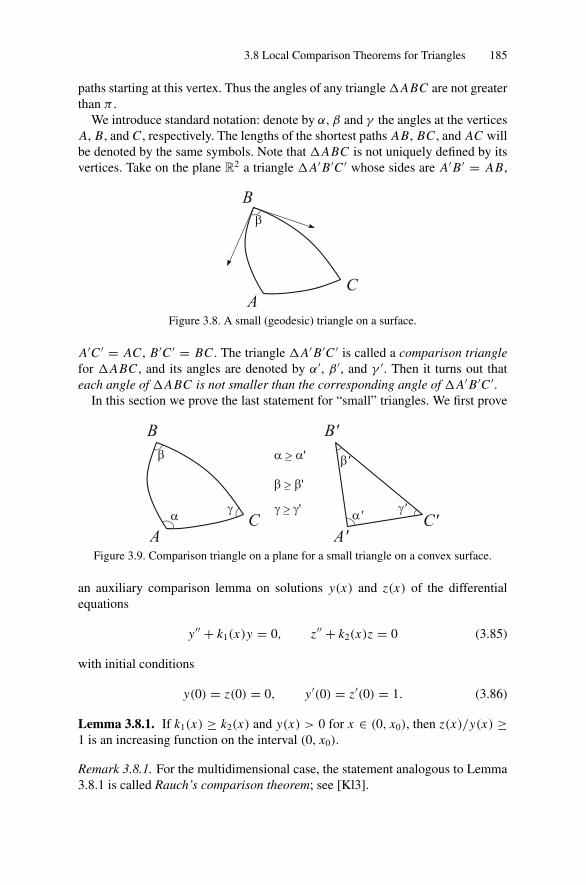
3.8 Local Comparison Theorems for Triangles 185
paths starting at this vertex. Thus the angles of any triangle �ABC are not greaterthan π .
We introduce standard notation: denote by α, β and γ the angles at the verticesA, B, and C , respectively. The lengths of the shortest paths AB, BC , and AC willbe denoted by the same symbols. Note that �ABC is not uniquely defined by itsvertices. Take on the plane R2 a triangle �A′ B ′C ′ whose sides are A′ B ′ = AB,
Figure 3.8. A small (geodesic) triangle on a surface.
A′C ′ = AC , B ′C ′ = BC . The triangle �A′ B ′C ′ is called a comparison trianglefor �ABC , and its angles are denoted by α′, β ′, and γ ′. Then it turns out thateach angle of �ABC is not smaller than the corresponding angle of �A′ B ′C ′.
In this section we prove the last statement for “small” triangles. We first prove
Figure 3.9. Comparison triangle on a plane for a small triangle on a convex surface.
an auxiliary comparison lemma on solutions y(x) and z(x) of the differentialequations
y′′ + k1(x)y = 0, z′′ + k2(x)z = 0 (3.85)
with initial conditions
y(0) = z(0) = 0, y′(0) = z′(0) = 1. (3.86)
Lemma 3.8.1. If k1(x) ≥ k2(x) and y(x) > 0 for x ∈ (0, x0), then z(x)/y(x) ≥1 is an increasing function on the interval (0, x0).
Remark 3.8.1. For the multidimensional case, the statement analogous to Lemma3.8.1 is called Rauch’s comparison theorem; see [Kl3].
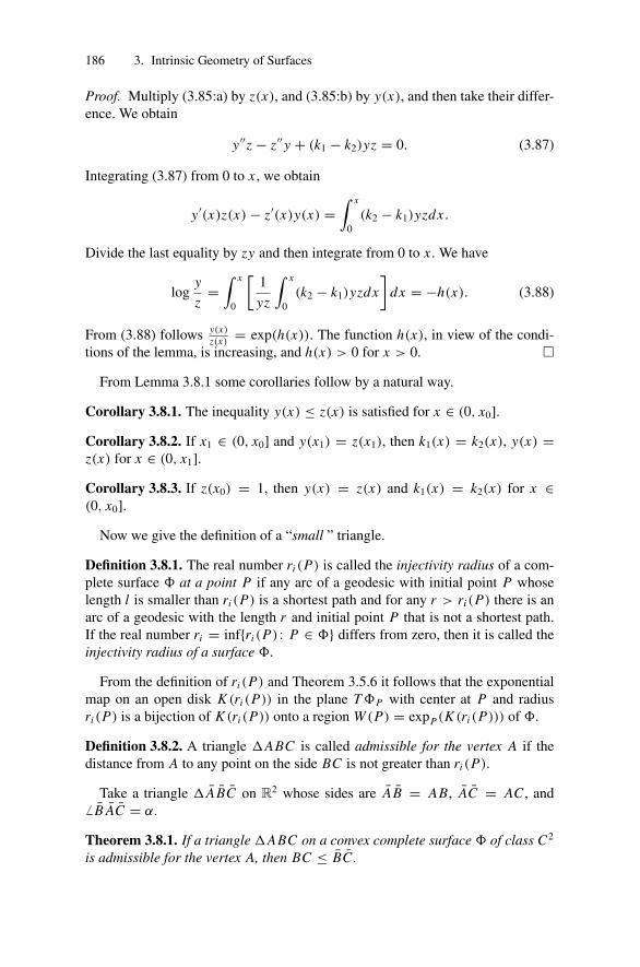
186 3. Intrinsic Geometry of Surfaces
Proof. Multiply (3.85:a) by z(x), and (3.85:b) by y(x), and then take their differ-ence. We obtain
y′′z − z′′y + (k1 − k2)yz = 0. (3.87)
Integrating (3.87) from 0 to x , we obtain
y′(x)z(x) − z′(x)y(x) =∫ x
0(k2 − k1)yzdx .
Divide the last equality by zy and then integrate from 0 to x . We have
logy
z=∫ x
0
[1
yz
∫ x
0(k2 − k1)yzdx
]dx = −h(x). (3.88)
From (3.88) follows y(x)
z(x)= exp(h(x)). The function h(x), in view of the condi-
tions of the lemma, is increasing, and h(x) > 0 for x > 0. �
From Lemma 3.8.1 some corollaries follow by a natural way.
Corollary 3.8.1. The inequality y(x) ≤ z(x) is satisfied for x ∈ (0, x0].Corollary 3.8.2. If x1 ∈ (0, x0] and y(x1) = z(x1), then k1(x) = k2(x), y(x) =z(x) for x ∈ (0, x1].Corollary 3.8.3. If z(x0) = 1, then y(x) = z(x) and k1(x) = k2(x) for x ∈(0, x0].
Now we give the definition of a “small ” triangle.
Definition 3.8.1. The real number ri (P) is called the injectivity radius of a com-plete surface � at a point P if any arc of a geodesic with initial point P whoselength l is smaller than ri (P) is a shortest path and for any r > ri (P) there is anarc of a geodesic with the length r and initial point P that is not a shortest path.If the real number ri = inf{ri (P) : P ∈ �} differs from zero, then it is called theinjectivity radius of a surface �.
From the definition of ri (P) and Theorem 3.5.6 it follows that the exponentialmap on an open disk K (ri (P)) in the plane T �P with center at P and radiusri (P) is a bijection of K (ri (P)) onto a region W (P) = expP(K (ri (P))) of �.
Definition 3.8.2. A triangle �ABC is called admissible for the vertex A if thedistance from A to any point on the side BC is not greater than ri (P).
Take a triangle � A BC on R2 whose sides are A B = AB, AC = AC , and� B AC = α.
Theorem 3.8.1. If a triangle �ABC on a convex complete surface � of class C2
is admissible for the vertex A, then BC ≤ BC .
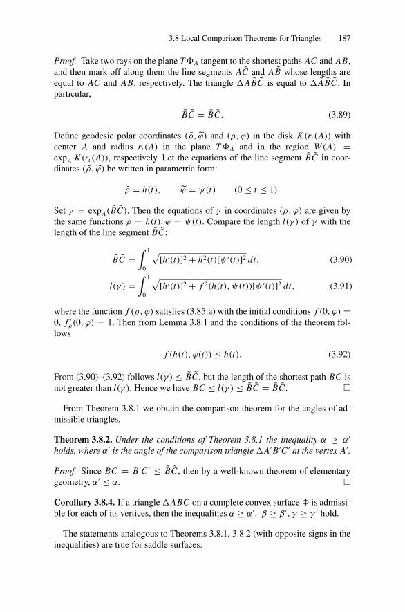
3.8 Local Comparison Theorems for Triangles 187
Proof. Take two rays on the plane T �A tangent to the shortest paths AC and AB,and then mark off along them the line segments AC and AB whose lengths areequal to AC and AB, respectively. The triangle �ABC is equal to � A BC . Inparticular,
BC = BC . (3.89)
Define geodesic polar coordinates (ρ, ϕ) and (ρ, ϕ) in the disk K (ri (A)) withcenter A and radius ri (A) in the plane T �A and in the region W (A) =expA K (ri (A)), respectively. Let the equations of the line segment BC in coor-dinates (ρ, ϕ) be written in parametric form:
ρ = h(t), ϕ = ψ(t) (0 ≤ t ≤ 1).
Set γ = expA(BC). Then the equations of γ in coordinates (ρ, ϕ) are given bythe same functions ρ = h(t), ϕ = ψ(t). Compare the length l(γ ) of γ with thelength of the line segment BC :
BC =∫ 1
0
√[h′(t)]2 + h2(t)[ψ ′(t)]2 dt, (3.90)
l(γ ) =∫ 1
0
√[h′(t)]2 + f 2(h(t), ψ(t))[ψ ′(t)]2 dt, (3.91)
where the function f (ρ, ϕ) satisfies (3.85:a) with the initial conditions f (0, ϕ) =0, f ′
ρ(0, ϕ) = 1. Then from Lemma 3.8.1 and the conditions of the theorem fol-lows
f (h(t), ϕ(t)) ≤ h(t). (3.92)
From (3.90)–(3.92) follows l(γ ) ≤ BC , but the length of the shortest path BC isnot greater than l(γ ). Hence we have BC ≤ l(γ ) ≤ BC = BC . �
From Theorem 3.8.1 we obtain the comparison theorem for the angles of ad-missible triangles.
Theorem 3.8.2. Under the conditions of Theorem 3.8.1 the inequality α ≥ α′holds, where α′ is the angle of the comparison triangle �A′ B ′C ′ at the vertex A′.
Proof. Since BC = B ′C ′ ≤ BC , then by a well-known theorem of elementarygeometry, α′ ≤ α. �
Corollary 3.8.4. If a triangle �ABC on a complete convex surface � is admissi-ble for each of its vertices, then the inequalities α ≥ α′, β ≥ β ′, γ ≥ γ ′ hold.
The statements analogous to Theorems 3.8.1, 3.8.2 (with opposite signs in theinequalities) are true for saddle surfaces.
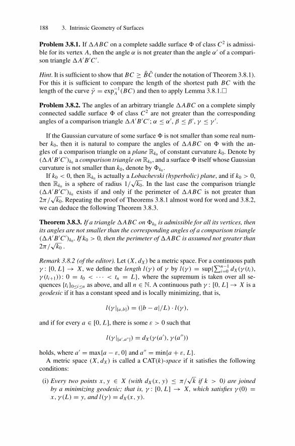
188 3. Intrinsic Geometry of Surfaces
Problem 3.8.1. If �ABC on a complete saddle surface � of class C2 is admissi-ble for its vertex A, then the angle α is not greater than the angle α′ of a compari-son triangle �A′ B ′C ′.
Hint. It is sufficient to show that BC ≥ BC (under the notation of Theorem 3.8.1).For this it is sufficient to compare the length of the shortest path BC with thelength of the curve γ = exp−1
A (BC) and then to apply Lemma 3.8.1.�
Problem 3.8.2. The angles of an arbitrary triangle �ABC on a complete simplyconnected saddle surface � of class C2 are not greater than the correspondingangles of a comparison triangle �A′ B ′C ′; α ≤ α′, β ≤ β ′, γ ≤ γ ′.
If the Gaussian curvature of some surface � is not smaller than some real num-ber k0, then it is natural to compare the angles of �ABC on � with the an-gles of a comparison triangle on a plane Rk0 of constant curvature k0. Denote by(�A′ B ′C ′)k0 a comparison triangle on Rk0 , and a surface � itself whose Gaussiancurvature is not smaller than k0, denote by �k0 .
If k0 < 0, then Rk0 is actually a Lobachevski (hyperbolic) plane, and if k0 > 0,then Rk0 is a sphere of radius 1/
√k0. In the last case the comparison triangle
(�A′ B ′C ′)k0 exists if and only if the perimeter of �ABC is not greater than2π/
√k0. Repeating the proof of Theorems 3.8.1 almost word for word and 3.8.2,
we can deduce the following Theorem 3.8.3.
Theorem 3.8.3. If a triangle �ABC on �k0 is admissible for all its vertices, thenits angles are not smaller than the corresponding angles of a comparison triangle(�A′ B ′C ′)k0 . If k0 > 0, then the perimeter of �ABC is assumed not greater than2π/
√k0 .
Remark 3.8.2 (of the editor). Let (X, dX ) be a metric space. For a continuous pathγ : [0, L] → X , we define the length l(γ ) of γ by l(γ ) = sup{∑n−1
i=0 dX (γ (ti ),γ (ti+1)) : 0 = t0 < · · · < tn = L}, where the supremum is taken over all se-quences {ti }0≤i≤n as above, and all n ∈ N. A continuous path γ : [0, L] → X is ageodesic if it has a constant speed and is locally minimizing, that is,
l(γ |[a,b]) = (|b − a|/L) · l(γ ),
and if for every a ∈ [0, L], there is some ε > 0 such that
l(γ |[a′,a′′]) = dX (γ (a′), γ (a′′))
holds, where a′ = max{a − ε, 0} and a′′ = min{a + ε, L}.A metric space (X, dX ) is called a CAT(k)-space if it satisfies the following
conditions:
(i) Every two points x, y ∈ X (with dX (x, y) ≤ π/√
k if k > 0) are joinedby a minimizing geodesic; that is, γ : [0, L] → X, which satisfies γ (0) =x, γ (L) = y, and l(γ ) = dX (x, y).
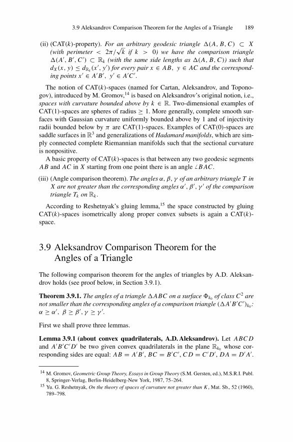
3.9 Aleksandrov Comparison Theorem for the Angles of a Triangle 189
(ii) (CAT(k)-property). For an arbitrary geodesic triangle �(A, B, C) ⊂ X(with perimeter < 2π/
√k if k > 0) we have the comparison triangle
�(A′, B ′, C ′) ⊂ Rk (with the same side lengths as �(A, B, C)) such thatdX (x, y) ≤ dRk (x ′, y′) for every pair x ∈ AB, y ∈ AC and the correspond-ing points x ′ ∈ A′ B ′, y′ ∈ A′C ′.
The notion of CAT(k)-spaces (named for Cartan, Aleksandrov, and Topono-gov), introduced by M. Gromov,14 is based on Aleksandrov’s original notion, i.e.,spaces with curvature bounded above by k ∈ R. Two-dimensional examples ofCAT(1)-spaces are spheres of radius ≥ 1. More generally, complete smooth sur-faces with Gaussian curvature uniformly bounded above by 1 and of injectivityradii bounded below by π are CAT(1)-spaces. Examples of CAT(0)-spaces aresaddle surfaces in R3 and generalizations of Hadamard manifolds, which are sim-ply connected complete Riemannian manifolds such that the sectional curvatureis nonpositive.
A basic property of CAT(k)-spaces is that between any two geodesic segmentsAB and AC in X starting from one point there is an angle � B AC .
(iii) (Angle comparison theorem). The angles α, β, γ of an arbitrary triangle T inX are not greater than the corresponding angles α′, β ′, γ ′ of the comparisontriangle Tk on Rk .
According to Reshetnyak’s gluing lemma,15 the space constructed by gluingCAT(k)-spaces isometrically along proper convex subsets is again a CAT(k)-space.
3.9 Aleksandrov Comparison Theorem for theAngles of a Triangle
The following comparison theorem for the angles of triangles by A.D. Aleksan-drov holds (see proof below, in Section 3.9.1).
Theorem 3.9.1. The angles of a triangle �ABC on a surface �k0 of class C2 arenot smaller than the corresponding angles of a comparison triangle (�A′ B ′C ′)k0 :α ≥ α′, β ≥ β ′, γ ≥ γ ′.
First we shall prove three lemmas.
Lemma 3.9.1 (about convex quadrilaterals, A.D. Aleksandrov). Let ABC Dand A′ B ′C ′ D′ be two given convex quadrilaterals in the plane Rk0 whose cor-responding sides are equal: AB = A′ B ′, BC = B ′C ′, C D = C ′ D′, D A = D′ A′.
14 M. Gromov, Geometric Group Theory, Essays in Group Theory (S.M. Gersten, ed.), M.S.R.I. Publ.8, Springer-Verlag, Berlin-Heidelberg-New York, 1987, 75–264.
15 Yu. G. Reshetnyak, On the theory of spaces of curvature not greater than K , Mat. Sb., 52 (1960),789–798.

190 3. Intrinsic Geometry of Surfaces
Figure 3.10. Comparison triangle (�A′ B′C ′)k0 for a triangle on a surface.
�
Then if the angle � ADC is not smaller (greater) than � A′ D′C ′, then � B AD and� BC D are not greater (smaller) than � B ′ A′ D′ and � B ′C ′ D′, respectively. For thecase k0 > 0 we assume that the perimeter of ABC D is smaller than 2π/
√k0. The
case that � ADC is equal to π also is not excluded.
Proof. Let k0 = 0. The conditions of the lemma implies that inequality AC ≥A′C ′ (AC > A′C ′), from which it follows that � ABC is not smaller (greater) than� A′ B ′C ′. But the sum of all angles of the quadrilaterals ABC D and A′ B ′C ′ D′is 2π . Therefore, at least one of the angles � B AD or � BC D does not exceed (issmaller than) � B ′ A′ D′ or � B ′C ′ D′. In both cases we have B D ≤ B ′ D′ (B D <
B ′ D′), whence the statement of the lemma follows.In the case of k0 �= 0 consider a quadrilateral A′′ B ′′C ′′ D′′ for which � A′′ D′′C ′′
= � A′ D′C ′, � B ′′C ′′ D′′ = � BC D, and the sides A′′ D′′, D′′C ′′ and C ′′ B ′′ areequal, respectively, to AD, DC , and C B. Comparing this quadrilateral withABC D and A′ B ′C ′ D′, one can see that � BC D does not exceed (is smaller than)� B ′C ′ D′.16 Similarly for the second inequality, whence it follows that � B ADdoes not exceed (is smaller than) � B ′ A′ D′. �
Remark 3.9.1. From the law of cosines of spherical and hyperbolic trigonometry(k0 = ±1),
cos a = cos b cos c + sin a sin b cos A,
cosh a = cosh b cosh c − sinh a sinh b cos A
it follows that in all cases that a = a(A) is a monotonic increasing function ofthe angle A ∈ [0, π ] when b, c are given. This simple fact on the monotonicityrelation between angle and length of the closing edge of a geodesic hinge in Rk0
can be used in the proof of Lemma 3.9.1, case k0 �= 0. (A geodesic hinge in � isa figure consisting of a point A ∈ � called the vertex and minimal geodesics γ, τ
emanating from A called sides. The angle between the tangent vectors to γ, τ atA is called the angle of the geodesic hinge.)
16 �B′′C ′′ D′′ = �BC D; hence B′′ D′′ = B D and � A′′ D′′ B′′ ≥ � ADB. Comparing �A′′ D′′ B′′with �ADB, we get A′′ B′′ ≤ AB (see Remark 3.9.1 by editor). Comparing �A′′ B′′C ′′ with�A′ B′C ′, from A′ B′ ≥ A′′ B′′ we get � A′C ′ B′ ≥ � A′′C ′′ B′′. Then � D′′C ′′ B′′ ≤ � D′C ′ B′.Comparing �B′C ′ D′ with �BC D, we get D′ B′ ≥ DB.
3.9 Aleksandrov Comparison Theorem for the Angles of a Triangle 191
Let D be an open region on � whose closure is compact, with a triangle �ABCin its interior, and d an elementary length of D (see Theorem 3.5.4).
Definition 3.9.1. A triangle �ABC is a thin triangle if the distance from anypoint on the side AB up to the side AC does not exceed δ = d/4.
Lemma 3.9.2. (about thin triangles.) If a triangle �ABC on a surface �k0 isthin, then its angles at the vertices B and C are not smaller than the correspondingangles of a comparison triangle (�A′ B ′C ′)k0 : β ≥ β ′, γ ≥ γ ′. In the case k0 > 0,the perimeter of �ABC is supposed to be not greater than 2π/
√k0.
Proof. Introduce the parameterizations B(x) and C(y) on the shortest paths ABand AC , where x and y are the lengths of the arcs AB(x) and AC(y) of the short-est paths AB and AC . Denote by β(x, y) and γ (x, y) the angles of �AB(x)C(y)
at the vertices B(x) and C(y), respectively. Define the set T of ordered pairs(x, y) by the following conditions:
(1) The angles β(x, y) and γ (x, y) are not smaller than the corresponding anglesβ ′(x, y) and γ ′(x, y) of a comparison triangle (�A′ B ′C ′)k1 , where k1 is anarbitrary real number smaller than k0.
(2) |x − y| ≤ δ/2.(3) If a pair (x1, y1) is in T , then (x2, y2) is also in T when x2 ≤ x1, y2 ≤ y1, and
|x2 − y2| ≤ δ/2.
From Corollary 3.8.4 it follows that the pairs (x, y) for x < δ/2 and y < δ/2belong to T . Consequently, the set T is nonempty. Define on T the functionf (x, y) = x + y. Let T0 = max{ f (x, y) : (x, y) ∈ T }. If T0 = AB + AC ,then the statement of the lemma has been proved. Assume that T0 = x0 + y0 <
AB + AC and derive a contradiction. Let, for definiteness, x0 ≥ y0. Then provethat the angle β(x, y) is greater than the angle β ′(x, y). Indeed, all the anglesof �B(x0 − δ/2)B(x0)C(y0) are greater than the corresponding angles of thetriangle (�B ′(x0 − δ/2)B ′(x0)C ′(y0))k1 (see Corollary 3.8.4 and the conditionfor k1). Therefore, the angle at the vertex B ′(x0 − δ/2) of the convex quadri-lateral A′′ B ′′(x0 − δ/2)B ′′(x0)C ′′(y0) in the plane Rk1 obtained by gluing tri-angles (�A′ B ′(x0 − δ/2)C ′(y0))k1 and (�B(x0 − δ/2)B(x0)C(y0))k1 to eachother along their common side B ′(x0 − δ/2)B ′(x0) is smaller than π . ApplyingLemma 3.9.1 to the quadrilateral A′′ B ′′(x0 − δ/2)B ′′(x0)C ′′(y0) and the trian-gle (�A′ B ′(x0)C ′(y0))k1 , we obtain our statement β(x0, y0) > β ′(x0, y0). Fromthe last inequality and continuity follows the existence of δ1 > 0 such that for0 ≤ t ≤ δ1 the angle β(x0, y0 + t) is not smaller than β ′(x0, y0 + t).
We prove that the pair (x0, y0+t) for 0 ≤ t ≤ min{δ1, δ, AC−y0} = δ2 belongsto T . Indeed, all angles of �B(x0)C(y0+t)C(y0) are greater than the correspond-ing angles of the triangle (�B ′(x0)C ′(x0+t)C ′(y0))k1 . Therefore, arguments sim-ilar to those stated above show us that the angle γ (x0, y0 + t) is greater thanγ ′(x0, y0 + t) for 0 ≤ t ≤ δ2. But then f (x0, y0 + t) = x0 + y0 + t > x0 + y0 = T0
for t > 0, contrary to the definition of T0. The statement of the lemma now fol-lows from the arbitrariness of k1. �
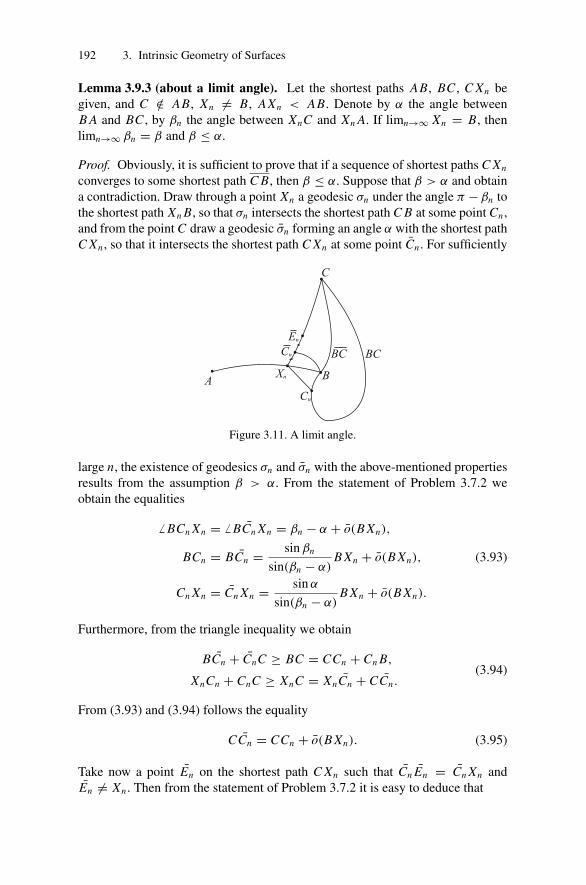
192 3. Intrinsic Geometry of Surfaces
Lemma 3.9.3 (about a limit angle). Let the shortest paths AB, BC , C Xn begiven, and C /∈ AB, Xn �= B, AXn < AB. Denote by α the angle betweenB A and BC , by βn the angle between XnC and Xn A. If limn→∞ Xn = B, thenlimn→∞ βn = β and β ≤ α.
Proof. Obviously, it is sufficient to prove that if a sequence of shortest paths C Xn
converges to some shortest path C B, then β ≤ α. Suppose that β > α and obtaina contradiction. Draw through a point Xn a geodesic σn under the angle π −βn tothe shortest path Xn B, so that σn intersects the shortest path C B at some point Cn ,and from the point C draw a geodesic σn forming an angle α with the shortest pathC Xn , so that it intersects the shortest path C Xn at some point Cn . For sufficiently
Figure 3.11. A limit angle.
large n, the existence of geodesics σn and σn with the above-mentioned propertiesresults from the assumption β > α. From the statement of Problem 3.7.2 weobtain the equalities
� BCn Xn = � BCn Xn = βn − α + o(B Xn),
BCn = BCn = sin βn
sin(βn − α)B Xn + o(B Xn), (3.93)
Cn Xn = Cn Xn = sin α
sin(βn − α)B Xn + o(B Xn).
Furthermore, from the triangle inequality we obtain
BCn + CnC ≥ BC = CCn + Cn B,
XnCn + CnC ≥ XnC = XnCn + CCn.(3.94)
From (3.93) and (3.94) follows the equality
CCn = CCn + o(B Xn). (3.95)
Take now a point En on the shortest path C Xn such that Cn En = Cn Xn andEn �= Xn . Then from the statement of Problem 3.7.2 it is easy to deduce that
3.9 Aleksandrov Comparison Theorem for the Angles of a Triangle 193
C En = 2Cn Xn sin(π
2− βn − α
2
)+ o(B Xn)
= 2Cn Xn cos(βn − α
2
)+ o(B Xn).
From this equality and from (3.95) follows
CCn + Cn B = C B ≤ C En + EnC
= 2Cn Xn cos(βn − α
2
)+ EnC + o(B Xn)
= 2Cn Xn cos(βn − α
2
)+ CCn − Cn Xn + o(B Xn). (3.96)
Further on, from (3.93), (3.95), and (3.96) we obtain the inequality
2CCn ≤ 2Cn Xn cos(βn − α
2
)+ o(B Xn)
= 2CCn cos(βn − α
2
)+ o(B Xn).
(3.97)
Divide (3.97) by 2CCn and pass to the limit for n → ∞. Then we obtain 1 ≤cos
(β−α
2
), which is impossible, since β − α > 0. �
3.9.1 Proof of the Comparison Theorem for theAngles of a Triangle
Let �ABC be an arbitrary triangle on a surface �k0 . In the case of k0 > 0 weassume temporarily that the perimeter of �ABC is smaller than 2π/
√k0. We
prove the theorem for the angle α. Introduce on AC a parameterization C(x),where x is the length of an arc AC(x) of shortest path. Denote by γ (x) the angle� AC(x)B of the triangle �ABC . Define the set of real numbers T of x satisfyingthe following inequalities:
α ≥ α′, γ ≥ γ ′ (3.98)
The set T is not empty, since by virtue of the lemma about thin triangles andthe lemma about a limit angle, the inequalities (3.98) are satisfied for sufficientlysmall x . Let x0 = sup T . If x0 = AC , then Theorem 3.8.1 is proven for theangle α.
Assume x0 < AC , and obtain a contradiction. Note that x0 ∈ T by the lemmaabout a limit angle. Take a sequence of points Cn = C(xn), Cn �= C(x0) =C0, xn > x0 such that limn→∞ Cn = C0. Also assume, without loss of general-ity, that the sequence of the shortest paths BCn converges to some shortest pathBC0. For sufficiently large n (n ≥ n0) the triangle �Cn0 BC0 is thin. Therefore,

194 3. Intrinsic Geometry of Surfaces
the angle at the vertex C0′′ of the quadrilateral A′′ B ′′Cn0
′′C0′′ obtained by glu-
ing (�A′ B ′Cn0′)k0 and (�Cn0
′ B ′C0′)k0 along their common side B ′C0
′ does notexceed π . Hence, from Lemma 3.9.1 it follows that xn0 ∈ T , contrary to the defi-nition of x0. So, Theorem 3.9.1 is proven for the angle α. For the other angles of�ABC , Theorem 3.9.1 can be proved similarly.
We are left to consider the case of k0 > 0 and remove from the assumption thatthe perimeter of �ABC is smaller than 2π/
√k0. Assume that on the surface �k0
there is a triangle �ABC whose perimeter is greater than 2π/√
k0, and obtain acontradiction. Suppose that at least one of the angles of �ABC , say the vertexA, differs from π . Take the points B0 and C0 on the sides AB and AC such thatAB0 + B0C0 + C0 A = 2π/
√k0. Assume, without loss of generality, that the sum
of the lengths of the two smallest sides of �AB0C0 is equal to the length of thethird. Let Bn and Cn be the sequences of points on AB and AC ; moreover, Bn �=B0, Cn �= C0, ABn < AB0, ACn < AC0, and limn→∞ Bn = B0, limn→∞ Cn =C0. Then for every t it is true that ABn + BnCn + Cn A < 2π/
√k0, for otherwise,
the perimeter of �ABC would be 2π/√
k0. Applying Theorem 3.9.1 to triangles�ABnCn , we obtain β ≥ β ′, γ ≥ γ ′. But as is easy to see, limn→∞ β ′
n =limn→∞ γ ′
n = π , and hence limn→∞ βn = limn→∞ γn = π . But then B0 BCC0
would be the shortest path of length 2π/√
k0, and consequently, the perimeter of�ABC would be 2π/
√k0, contrary to the assumption.
So we have proved that if the perimeter of �ABC is greater than 2π/√
k0, thenall its angles are π , which means that the line AB ∪ BC ∪C A is a closed geodesicγ . But then the perimeter of �A1 BC , where A1 ∈ γ and A1 also is close to A,is larger than 2π/
√k0, and its angles at the vertices B and C differ from π . The
obtained contradiction proves an absence on �k0 of a triangle whose perimeter isgreater than 2π/
√k0.
Now let the perimeter of �ABC be 2π/√
k0. If the triangle is nondegenerate,then reasoning as above, we can prove that �ABC is a closed geodesic, andconsequently, all its angles are π , and then the statements of Theorem 3.9.1 areobviously true. If it is degenerate, that is, composed of two shortest paths (a bi-angle (or lune)), then in this case the surface �k0 is a sphere (see Problem 3.10.1),and �ABC can be compared with itself.
The comparison theorem for the angles can formulated in a different form, us-ing the convexity condition of A.D. Aleksandrov. Let AB and AC be two shortestpaths starting from the point A, and also suppose B(x) ∈ AB, C(y) ∈ AC ,x = AB(x), y = AC(y). Denote by ϕ(x, y) the angle at the vertex A′ of acomparison triangle (�A′ B ′(x)C ′(y))k0 . We say that the Aleksandrov convexitycondition is satisfied on a surface � with respect to a plane Rk0 if the functionϕ(x, y) is decreasing.
Theorem 3.9.2. A surface �k0 satisfies the Aleksandrov convexity condition withrespect to Rk0 .
Proof. This theorem easily follows from Theorem 3.9.1 and Lemma 3.9.1. �

3.10 Problems to Chapter 3 195
3.10 Problems to Chapter 3
Problem 3.10.1. The diameter d of a surface �k0 (k0 > 0) is not greater thanπ/
√k0. If d = π/
√k0, then �k0 coincides with a sphere of radius 1/
√k0.
Solution. The first statement of Problem 3.10.1 obviously follows from Theo-rem 3.9.1. Consider the case d = π/
√k0. Let A and B be the endpoints of
a diameter, and P an arbitrary point on �k0 . Then, by the triangle inequality,AP + P B ≥ π/
√k0, but on the other hand, π/
√k0 + AP + P B ≤ 2π/
√k0.
Therefore, AP + P B = π/√
k0. From the last equality it follows that the polyg-onal line AP ∪ P B is a shortest path of length π/
√k0. Thus we have obtained
that any geodesic starting from A comes to B, and the length of an arc AB of thisgeodesic is π/
√k0. Introduce the geodesic polar coordinates (ρ, ϕ) with the ori-
gin at A. Then ds2 = dρ2+ f 2(ρ, ϕ)dϕ2, where the function f (ρ, ϕ) satisfies theequation f ′′
ρρ+K (ρ, ϕ) f = 0 with initial conditions f (0, ϕ) = 0, f ′ρ(0, ϕ) = 1.
From what we have proved it follows that f (ρ, ϕ) > 0 for 0 < ρ < π/√
k0, andsince sin(
√k0ρ)/
√k0 is zero at ρ = π/
√k0, then from the third corollary of
Lemma 3.8.1 it follows that K (ρ, ϕ) ≡ k0 for 0 ≤ ϕ ≤ 2π ; i.e., we have provedthat the Gaussian curvature at each point of the surface �k0 is the constant k0. Thestatement of Problem 3.10.1 now follows from Theorem 2.8.2 of Liebmann. �
Remark 3.10.1. In the conditions of Problem 3.10.1 it is possible to construct anisometry ψ : �k0 → S(1/
√k0) and not use Liebmann’s theorem. So this problem
is solved for the multidimensional case. The reader is asked to prove that expA isthe required isometry ψ .
Recall that a straight line on a surface is a complete geodesic γ such that everyone of its arcs is a shortest path.
Problem 3.10.2 (S. Cohn-Vossen). Prove that if on a complete convex surfaceof class C2 there is a straight line γ , then � is a cylinder.
Solution. Take an arbitrary point P ∈ �, P ∈ γ . Let γP be a point on γ , thenearest to P . Then the shortest path PγP is either orthogonal to γ , or P can bejoined with a point γP at least by two shortest paths, each of which forms withγ an angle not greater than π/2 (see Lemma 3.5.1). Let γ (t) be a parameteri-zation of γ and t = ±γPγ (t), γP = γ (0), −∞ < t < ∞, tn be a sequenceof positive numbers tending to infinity, and τn a sequence of negative numberstending to minus infinity. Without loss of generality, assume that the limit of theshortest paths Pγ (tn) for n → ∞ is some ray σ1 with vertex at P , and the limitof the shortest paths Pγ (τn) for c is some ray σ2 with the same vertex P . Placethe triangles �P ′γ ′(tn)γ ′(τn) on R2 so that the sides γ ′(tn)γ ′(τn) lie on the samestraight line a. From Theorem 3.9.1 and Lemma 3.9.1 it follows that the dis-tance from the vertex P ′ of triangle �P ′γ ′(tn)γ ′(τn) up to a straight line a doesnot exceed PγP for any n. Therefore, the limit of the angle � γ ′(tn)P ′γ ′(τn) forn → ∞ is π ; i.e., the rays σ1 and σ2 lie on the same geodesic γ . But then from

196 3. Intrinsic Geometry of Surfaces
Theorem 3.9.1 it follows that the angle between σ1 and σ2 is also π , since therays σ1 and σ2 lie on the same geodesic γ . Furthermore, the sum of the angles� P ′γ ′(0)γ ′(tn) and � γ ′(0)P ′γ ′(tn) of �γ ′(0)P ′γ ′(tn) for n → ∞ is equal to π ,and since � P ′γ ′(0)γ ′(tn) does not exceed π/2 (by Theorem 3.9.1) for any n, thelimit of the angle � γ ′(0)P ′γ ′(tn) for n → ∞ is not smaller than π/2. Then againby Theorem 3.9.1, an angle between the ray σ1 and the shortest path Pγ (0) is notsmaller than π/2. It can be proved similarly that the angle between σ2 and Pγ (0)
is not smaller than π/2. But since their sum is π , we obtain that Pγ (0) intersectsγ in a right angle. From here it follows that a shortest path Pγ (0) also intersectsthe geodesic γ in a right angle.
Now let P1 ∈ γ and P1 �= P . Repeating all the previous constructions andreasoning, we obtain that the shortest path P1γP1 intersects the geodesics γ andγ also in a right angle. So, we have obtained that in the region D bounded bythe quadrilateral P P1γP1γP , all internal angles are π/2. Applying to region D theGauss–Bonnet formula, we obtain that the integral curvature of D is zero. But theGaussian curvature of the surface � is nonnegative; consequently, it is identicallyzero at each point of D. In particular, the Gaussian curvature of � is zero at P .But the point P has been selected arbitrarily. Hence the Gaussian curvature of �
is zero at every point. �
Remark 3.10.2. In Problem 3.10.2 as well as in Problem 3.10.1 it is possibleto construct an isometry ψ of � onto the plane R0 without referring to theGauss–Bonnet theorem. Namely, these arguments solve this problem in the n-dimensional case. To construct a map ψ , one needs to introduce a semigeodesiccoordinate system on � and R0 and to compare points with identical coordinates.
Problem 3.10.3. For a triangle �ABC on a surface �k0 let the shortest path ABbe a unique shortest path connecting points A and B, and let the angle γ be equalto the angle γ ′. Prove that then all angles of �ABC are equal to the correspondingangles of (�ABC)k0 .
Hint. It is sufficient to prove that for any point P on the shortest path AC theangle � B PC is equal to � B ′ P ′C ′ of triangle (�B ′ P ′C ′)k0 , which follows easilyfrom Theorem 3.9.1 and Lemma 3.9.1. After this, it is easy to prove that α = α′.The equality β = β ′ is proved analogously.
Problem 3.10.4. Prove that in the conditions of Problem 3.10.3, �ABC boundsa region such that at every one of its points the Gaussian curvature is k0.
Hint. Use the results of Problem 3.10.3, Lemma 3.5.1, and Lemma 3.8.1.
Problem 3.10.5. Let �ABC be composed of the shortest paths AB, BC , and anarc AC of a geodesic whose length is smaller than AB + BC . Prove that α ≥ α′and γ ≥ γ ′.
Hint. Divide a geodesic AC into a finite number of arcs, each of them a shortestpath, and take advantage of Theorem 3.9.1 and Lemma 3.9.1.
3.10 Problems to Chapter 3 197
Problem 3.10.6. Prove that on a surface �k0 for k0 > 0 each arc of a geodesicwhose length is greater than 4π/
√k0 has points of self-intersection.
Hint. Assume the opposite and with the help of Theorem 3.9.1 reduce this as-sumption to a contradiction.
Problem 3.10.7. For �ABC on a surface �k0 with k0 > 0 construct a triangle(�A′′ B ′′C ′′)k0 whose angles are equal to the corresponding angles of �ABC .Prove that then AB ≤ A′′ B ′′, AC ≤ AC ′′, BC ≤ B ′′C ′′. Consider the case inwhich AB = A′′ B ′′ and the angles of �ABC at the vertices A and B are equal tothe angles of �A′′ B ′′C ′′ at the vertices A′′ and B ′′.
Problem 3.10.8. Formulate and solve the problems for saddle surfaces analogousto Problems 3.10.3 and 3.10.4.
Problem 3.10.9. Let Kr be a disk of radius r with center at a point O on a convexsurface �, and let AB be a chord of this disk. Prove that if � O AB = � O B A =45◦, then AB ≥ √
2r .
Problem 3.10.10. Let r be some ray with vertex at a point P on a completeconvex surface � of class C2. Introduce on r a parameterization r(t), where t isthe arc length parameter counted from P . Let B(t) = {Q ∈ � : ρ(Q, r(t)) < t}.Prove that D(r) = �\⋃∞
t=0 B(t) is an absolutely convex set on � for any ray r .
Problem 3.10.11. Let � be a complete regular surface of class C2 whose Gaus-sian curvature satisfies the inequality 1
a2 ≤ K ≤ 1. Prove that there is a diffeo-morphism ϕ of � onto a unit sphere S1 such that for any points P and Q on �,the following inequalities satisfied:
ρ1(ϕ(P), ϕ(Q)) ≤ ρ�(P, Q) ≤ aρ1(ϕ(P), ϕ(Q)).
Here ρ1 is a metric on S1, and ρ� is a metric on �.
Remark 3.10.3. The construction of diffeomorphisms satisfying the first and sec-ond inequality separately is simple enough. But it is not known whether thereexists a diffeomorphism ϕ satisfying both these inequalities.
Note that all theorems and problems of Sections 3.9, 3.10 can be formulatedand proved for any geodesically convex region on a regular surface of class C2.
References
[AlZ] Aleksandrov A.D. and Zalgaller V.A. Intrinsic geometry of surfaces.Translations of Mathematical Monographs, v. 15. Providence, RI: Amer-ican Mathematical Society. VI, 1967.
[Bl] Blaschke W. and Leichtweiss K. Elementare Differentialgeometrie.Berlin-Heidelberg-New York: Springer-Verlag. X, 1973.
[Bus] Busemann H. Convex Surfaces. Interscience Tracts in Pure and AppliedMathematics. 6. New York–London: Interscience Publishers, 1958.
[Cohn] Cohn-Vossen S.E. Verbiegbarkeit der Flachen im Grossen. Uspechi Mat.Nauk, vol. 1, 33–76, 1936.
[Gau] Gauss C.F. General Investigations of Curved Surfaces. Hewlett, NY:Raven Press, 1965.
[Hop] Hopf H. Differential Geometry in the Large. 2nd ed. Lecture Notes inMathematics, Vol. 1000. Berlin etc.: Springer-Verlag, 1989.
[Kl1] Klingenberg W. Riemannian Geometry. 2nd ed. de Gruyter Studies inMathematics. Berlin: Walter de Gruyter, 1995.
[Kl2] Klingenberg W. A Course in Differential Geometry. Corr. 2nd print.Graduate Texts in Mathematics, v. 51. New York–Heidelberg–Berlin:Springer-Verlag. XII, 1983.
[Kl3] Gromoll D., Klingenberg W. and Meyer W. Riemannsche Geometrieim Grossen. Lecture Notes in Mathematics. 55. Berlin-Heidelberg-NewYork: Springer-Verlag, VI, 1975.
[Ku1] Kutateladze S.S. (ed). A.D. Alexandrov Selected Works. Part 2: IntrinsicGeometry of Convex Surfaces. New York; London: Taylor & Francis,2004.
[Miln] Milnor J. Morse Theory. Annals of Mathematics Studies. No. 51, Prince-ton, Princeton University Press, VI, 1963.
200 References
[Top] Toponogov V.A. Riemannian spaces having their curvature bounded be-low by a positive number. Dokl. Akad. Nauk SSSR, vol. 120, 719–721,1958.
[Pog] Pogorelov A.V. Extrinsic Geometry of Convex Surfaces. Translations ofMathematical Monographs, Vol. 35. Providence, American Mathemati-cal Society, VI, 1973.
[Sto] Stoker, J.J. Differential Geometry. Pure and Applied Mathematics. Vol.XX. New York etc.: Wiley-Interscience, 1969.
Additional Bibliography:
Differential Geometry of Curves and Surfaces
[Am1] Aminov Yu. Differential Geometry and Topology of Curves. Amsterdam:Gordon and Breach Science Publishers, 2000.
[BG] Berger M. and Gostiaux, B. Differential Geometry: Manifolds, Curvesand Surfaces. New York: Springer-Verlag, 1988.
[Blo] Bloch E.D. A First Course in Geometric Topology and Differential Ge-ometry. Boston: Birkhauser, 1997.
[Cas] Casey J. Exploring Curvature. Wiesbaden: Vieweg, 1996.[doC1] do Carmo M. Differential Geometry of Curves and Surfaces. Englewood
Cliffs, NJ: Prentice Hall, 1976.[Gra] Gray A. A Modern Differential Geometry of Curves and Surfaces. Sec-
ond Edition, CRC Press, Boca Raton 1998.[Hen] Henderson D.W. Differential Geometry: A Geometric Introduction. Up-
per Saddle River, NJ: Prentice Hall, 1998.[Hic] Hicks N.J. Notes of Differential Geometry. New York: Van Nostrand
Reinhold Company,1971.[Kre] Kreyszig E. Differential Geometry (Mathematical Expositions No. 11),
2nd Edition. Toronto: University of Toronto Press, 1964.[Mill] Millman R.S. and Parker G.D. Elements of Differential Geometry. En-
glewood Cliffs, NJ: Prentice-Hall, 1977.[Opr] Oprea J. Introduction to Differential Geometry and Its Applications. Up-
per Saddle River: Prentice Hall, 1997.[Pra] Prakash N. Differential Geometry: An Integrated Approach. New Delhi:
Tata McGraw-Hill, 1993.[Pre] Pressley A. Elementary Differential Geometry. Springer-Verlag, 2001.[Rov1] Rovenski V.Y. Geometry of Curves and Surfaces with MAPLE. Boston,
Birkhauser, 2000.[Shi] Shikin E.V. Handbook and atlas of curves. Boca Raton, FL: CRC Press.
xiv, 1995.[Tho] Thorpe J.A. Elementary Topics in Differential Geometry. Undergraduate
Texts in Mathematics. Corr. 4th printing, Springer-Verlag. 1994.

References 201
Riemannian Geometry
[Am] Aminov Yu. The Geometry of Submanifolds. Amsterdam: Gordon andBreach Science Publishers, 2001.
[Ber] Berge M. A Panoramic View of Riemannian Geometry. Berlin: Springer,2003.
[BCO] Berndt J., Console S. and Olmos C. Submanifolds and Holonomy. Chap-man & Hall/CRC Research Notes in Mathematics 434. Boca Raton, FL:Chapman and Hall/CRC, 2003.
[Bes2] Besse A.L. Einstein Manifolds. Springer, Berlin-Heidelberg-New York,1987.
[BH] Bridson M.R. and Haefliger A. Metric Spaces of Non-Positive Curva-ture. Fundamental Principles of Mathematical Sciences, 319. Springer-Verlag, 2001.
[BZ] Burago Yu.D. and Zalgaller V.A. Geometric Inequalities. Transl. fromthe Russian by A. B. Sossinsky. Grundlehren der Mathematischen Wis-senschaften, 285. Berlin etc.: Springer-Verlag. XIV, 1988.
[BBI] Burago D., Burago Yu. and Ivanov S. A Course in Metric Geometry.Graduate Studies in Mathematics. Vol. 33. Providence, RI: AMS, 2001.
[Chen1] Chen, Bang-yen Geometry of Submanifolds. Pure and Applied Mathe-matics. 22. New York: Marcel Dekker, Inc., 1973.
[Chen2] Chen, Bang-yen Geometry of Submanifolds and Its Applications. Tokyo:Science University of Tokyo. III, 1981.
[Cao] Cao J. A Rapid Course in Modern Riemannian Geometry. Ave MariaPress, 2004.
[doC2] do Carmo M. Riemannian Geometry. Boston: Birkhauser, 1992.[Car1] Cartan, E. Geometry of Riemannian Spaces. Transl. from the French by
J. Glazebrook. Notes and appendices by R. Hermann. Brookline, Mas-sachusetts: Math Sci Press. XIV, 1983.
[Car2] Cartan, E. Riemannian geometry in an orthogonal frame. From lecturesdelivered by Elie Cartan at the Sorbonne 1926–27. With a preface tothe Russian edition by S.P. Finikov. Translated from the 1960 Russianedition by V.V. Goldberg and with a foreword by S.S. Chern.
[Cha] Chavel I., et al. Riemannian Geometry: A Modern Introduction. (Cam-bridge Tracts in Mathematics). Cambridge University Press. Cambridge,1993.
[CE] Cheeger, J. and Ebin, D. Comparison Theorems in Riemannian Geome-try. Elsevier, 1975.
[DFN] Dubrovin B.A., Fomenko A.T., Novikov S.P. Modern Geometry: Meth-ods and Applications Robert G. Burns, trans., New York: Springer-Verlag, 1984.
[Eis] Eisenhart L.P. Riemannian Geometry. Princeton University Press, Princ-ton, N.J. 1997 (originally published in 1926).
[GHL] Gallot S., Hulin D., Lafontaine J. Riemannian Geometry. Universitext.Springer-Verlag; 3rd edition. 2004.

202 References
[Jos] Jost J. Riemannian Geometry and Geometric Analysis. Springer-Verlag;3rd edition, 2001.
[KN] Kobayashi S. and Nomizu S. Foundations of Differential Geometry I, II.Wiley-Interscience, New York; New Edition, 1996.
[Lan] Lang S. Fundamentals of Differential Geometry. Vol. 191, Springer-Verlag, 1998.
[Lau] Laugwitz D. Differential and Riemannian Geometry. F. Steinhardt,trans., New York: Academic Press, 1965.
[Lee] Lee J. M. Riemannian Manifolds: An Introduction to Curvature. (Grad-uate Texts in Mathematics , Vol. 176). New York: Springer, 1997.
[Mey] Meyer W.T. Toponogov’s Theorem and Applications. Lecture Notes,College on Differential Geometry, Trieste, 1989. http://www.math.uni-muenster.de/math/u/meyer/publications/toponogov.html
[Mrg] Morgan F. Riemannian Geometry: A Beginner’s Guide. A.K. Peters Ltd,2nd edition, 1998.
[O’Neill] O’Neill B. Elementary Differential Geometry. Academic Press,London–New York, 1966.
[OG] Osserman, R., Gamkrelidze, R.V. (eds.) Geometry V: Minimal surfaces.Transl. from the Russian. Encyclopaedia of Mathematical Sciences. 90.Berlin: Springer, 1997.
[Pet] Petersen P. Riemannian Geometry. (Graduate Texts in Mathematics,171). Springer-Verlag, 1997.
[Pos] Postnikov M.M. Geometry VI · Riemannian Geometry. Encyclopaediaof Mathematical Sciences. Vol. 91. Berlin: Springer, 2001.
[Rov2] Rovenski V.Y. Foliations on Riemannian Manifolds and Submanifolds.Synthetic Methods. Birkhauser, 1997.
[Sak] Sakai T. Riemannian Geometry. American Mathematical Society, 1996.[Spi] Spivak M. A Comprehensive Introduction to Differential Geometry (5
Volumes). Publish or Perish, 1979.[Ste] Sternberg S. Lectures on Differential Geometry (2nd edition). Chelsea.
New York, 1982.[Wal] Walschap G. Metric Structures in Differential Geometry. Series: Gradu-
ate Texts in Mathematics, Vol. 224. Birkhauser, 2004.[Wil] William M.B. An Introduction to Differentiable Manifolds and Rieman-
nian Geometry. 2. Udgave, Academic Press, 1986.[Wilm] Willmore T.J. Riemannian Geometry. Oxford University Press, 1997.
Index
Aleksandrov convexity condition,194
base of a polygon, 36bi-angle (lune), 51, 184, 194Bonnet rigidity theorem, 132
canonical parameter (on ageodesic), 156
Christoffel symbolsof the first kind, 151of the second kind, 129, 151
Clairaut’s theorem, 123comparison triangle, 185
on the plane Rk0 , 188convex
region, 15, 106, 170region on a sphere, 51
Coordinatesgeodesic polar (on a surface), 175geographical, 78local (on a surface), 151Riemannian normal (on a
surface), 174semigeodesic (on a surface), 176
cosines, law of, 190covering map, 156Curve, 22
absolute torsion, 45arc length parameterization, 14astroid, 4, 63bicylinder, 6binormal vector, 11cardioid, 4catenary, 147central set, 37closed, 3conic helix, 3convex, 15convex on a sphere, 51convex, plane, 15curvature, 19cycloid, 3, 63diametrically opposite points, 44epicycloid, 3explicit presentation, 4graph, 4half-cubic (Neil’s) parabola, 42helix, 3, 15, 50, 51, 62, 122hypocycloid, 3
204 Index
implicit equations, 5implicit presentation, 5integral curvature, 54length, 11natural equation, 23normal line, 8parallel, 38parametric equations, 3parametric presentation, 4piecewise smooth (regular), 3principal normal vector, 10radius of curvature, 22rectifiable, 11, 14regular of class Ck , 2simple, 23smooth, 2smooth regular, 23tangent line, 6tractrix, 4, 63, 101, 147vector form equation, 3velocity vector, 6Viviani, 5width, 43
derivational formulas, 129differentiable field of unit normals,
71directrix plane, 102distance between the points, 51
element of arc length, 75equivalent local diffeomorphisms,
22Euler characteristic, 124, 183Euler system, 163Euler’s equations, 163Euler’s formula, 87evolute, 41evolvent, 42exponential map, 157
flat torus, 149Frenet formulas, 47
Gauss (spherical) map, 93
Gauss’s formula, 131geodesic, 120
equations, 156minimal, 164
geodesic curvature, 119, 159sign, 160
great circle, 93, 121
height function relative to the unitvector, 73
immersion, 96proper, 96
indicatrix of a tangent line, 54injectivity radius
at a point, 186of a surface, 186
interior angle from the side of aregion, 180
isometry, 76isoperimetric inequality, 18
Klein bootle, 149
Lobachevskii (hyperbolic) plane,188
Mobius strip, 71, 149
normal plane of a curve, 47
orientable plane, 73orientation of a region, induced by
coordinates, 179osculating plane of a curve, 8, 47
parallel of a surface of revolution,122
parallel translation along a curve,153
Peterson–Codazzi formulas, 131phase distance of two vectors, 57phase length, 58phase polygonal line inscribed in a
curve, 58
Index 205
Pointelliptic (of convexity), 80, 85hyperbolic (saddle), 80, 85parabolic (cylindrical), 85planar, 86umbilic, 86, 114
polygonal line, 11
rectifying plane of a curve, 47regular value of a map, 5regularly inscribed polygon in a
curve, 11Rello’s triangle, 43right-hand rule, 46ruling (of a ruled surface), 106, 122
secant, 8set of all curves in a region joining
two points, 170set of all regularly inscribed
polygonal lines in a curve, 11shortest path (on a sphere), 51sign of principal curvature, 82stationarity of a tangent plane, 105Surface, 65, 95
absolute parallelness, 154absolute parallelness on a region,
154absolutely convex region, 171angle of a triangle, 184area element, 77asymptotic curve, 117asymptotic direction, 117base curve, 105canonical neighborhood, 167catenoid, 148closed (compact), 76co-ray, 171complete, 76conoid, 102convex, 106convex region, 170coordinate curves, 67coordinate neighborhood, 66
covariant derivative of a vectorfield, 152
cylinder, 82, 122developable, 105disk, 175distance between points of a
region, 170distance between two points, 76,
161embedded, 95first fundamental form, 74Gaussian curvature, 85generalized cylinder, 127, 133generalized Plucker’s conoid,
103generalized torus, 127, 133geodesic, 156geodesic triangle, 184geodesically complete, 168geodesically convex region, 170helicoid, 102immersed, 95implicit equation, 66integral curvature of a region, 93intrinsic geometry, 75isometric, 76k-fold continuously
differentiable, 66parameterization, 65
line of curvature, 114local basis at a point, 73local coordinates of a point, 67mean curvature, 85metrical completeness, 169minimal, 86noncylindrical, 102nonorientable, 71normal, 70normal curvature, 79of nonpositive Gaussian
curvature, 184of revolution
indicatrix, 139orientable, 71parallel, 90
206 Index
parallel vector field along acurve, 153
parameterization, 65parametric equations, 66principal curvature at the point,
84principal vectors at the point, 84pseudosphere, 101, 148ray, 171regular, 66right helicoid, 82, 148, 150ruled, 102saddle, 111second fundamental form, 80set of all rectifiable curves with
given endpoints, 76
shortest path, 162shortest path in a region, 170simply connected, 184small triangle, 186straight line, 195tangent plane, 70Tchebyshev net, 139thin triangle, 191third fundamental form, 91totally convex region, 170triangle admissible for the vertex,
186Weingarten, 133, 139
two-dimensional manifold, 95
![Chapter 19 Basics of the Differential Geometry of Curvescis610/gma-v2-chap19.pdf530 19 Basics of the Differential Geometry of Curves wecanthinkoftheparametert ∈]a,b[ astime,andthefunction](https://img.pdfslide.us/doc/110x75/60c2171126d3013b755dc7ff/chapter-19-basics-of-the-differential-geometry-of-curves-cis610gma-v2-530-19-basics.jpg)