Dielectric PolarizationWe divide matter into two categories: conductors and insulators. Free charges in a conductor will respond to exactly cancel an applied field. The charges in an insulator will respond to an applied field in such a way as to partially cancel an applied electric field. The situation in an insulatoris more complicated, however, since a molecule in the insulator will also experience a field due to the response of the insulator. There is a reaction field due to the response of themedium to charges on the molecule and there is a local field due to polarization of the solvent in the applied field. These issues are important for relating the molecular polarizability to the bulk polarization. Here we shall demonstrate the role of the dielectric constant (also called the relative permittivity) as a factor that relates the polarization of an insulator to an applied electric field.

The Electric Field in a Capacitor

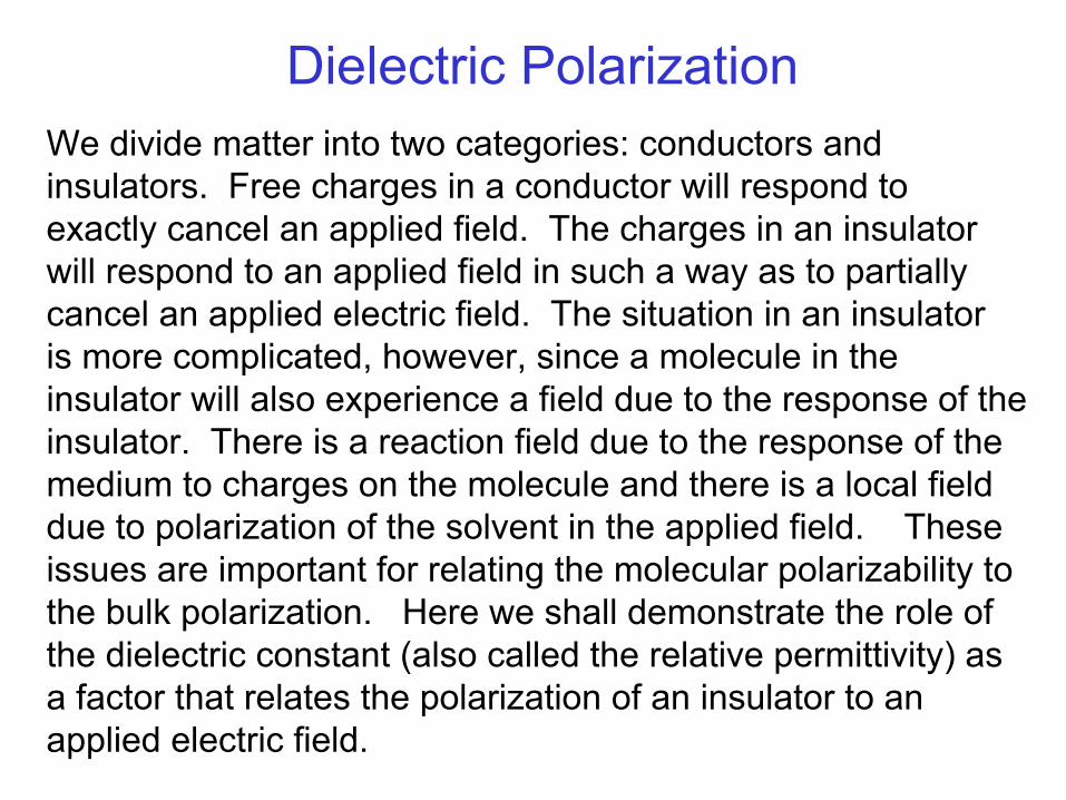
The experimental geometry that is most convenient for the purpose of demonstrating the dielectric constant is the parallel plate capacitor. We compare a capacitor with vacuum between the charged plates to one with a dielectric. In the case of vacuum the field is:

Notice that the way the field is defined, it is independent ofwhat is placed in the capacitor. Field calculations are simple.Just use the voltage and divide by the separation distance.Common units of field are V/cm or V/m.

E0 = σε0

= φdz

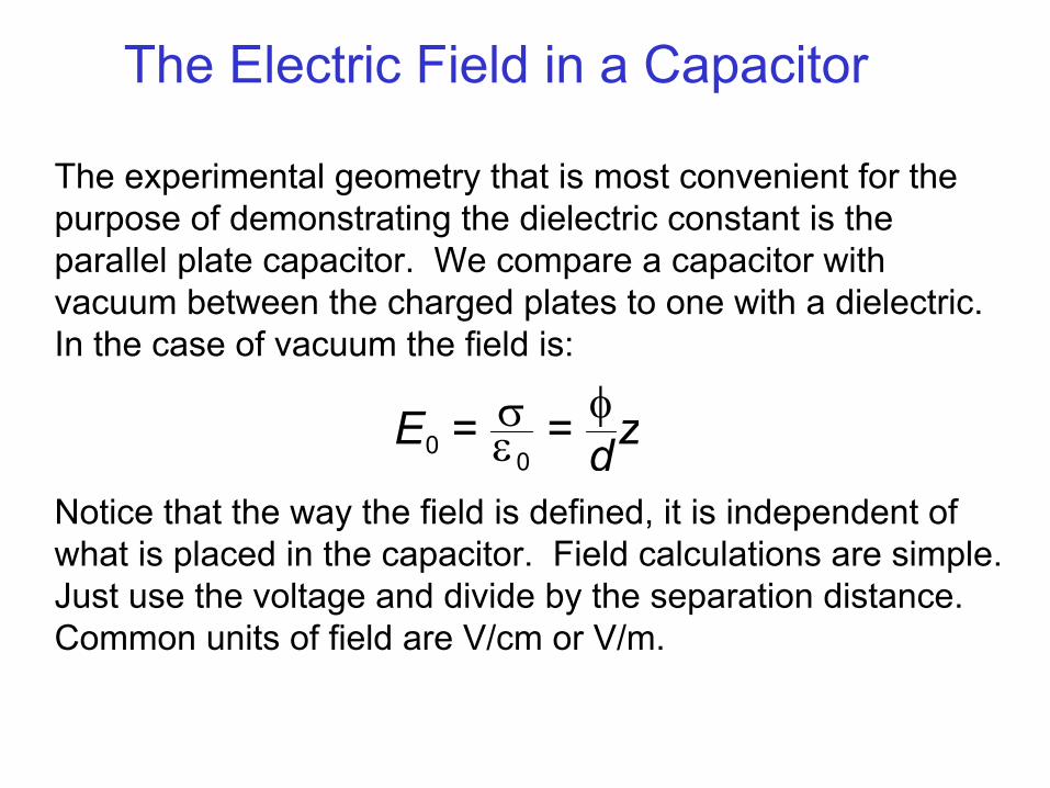
Illustration of the parallel plate capacitorThe surface charge density is σ = q/A. The vacuum permittivity is ε0. The potential is φ and the distance between the plates is d. The unit vector z is normal to the capacitor plates. These features are illustrated below.

z

A = area

dφ

grounded platecharged plate

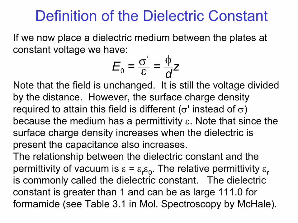
Definition of the Dielectric ConstantIf we now place a dielectric medium between the plates at constant voltage we have:

Note that the field is unchanged. It is still the voltage divided by the distance. However, the surface charge density required to attain this field is different (σ' instead of σ) because the medium has a permittivity ε. Note that since the surface charge density increases when the dielectric is present the capacitance also increases. The relationship between the dielectric constant and the permittivity of vacuum is ε = εrε0. The relative permittivity εris commonly called the dielectric constant. The dielectric constant is greater than 1 and can be as large 111.0 for formamide (see Table 3.1 in Mol. Spectroscopy by McHale).

E0 = σ′

ε = φdz

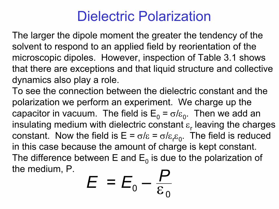
Dielectric PolarizationThe larger the dipole moment the greater the tendency of the solvent to respond to an applied field by reorientation of the microscopic dipoles. However, inspection of Table 3.1 shows that there are exceptions and that liquid structure and collective dynamics also play a role. To see the connection between the dielectric constant and the polarization we perform an experiment. We charge up the capacitor in vacuum. The field is E0 = σ/ε0. Then we add an insulating medium with dielectric constant εr leaving the charges constant. Now the field is E = σ/ε = σ/εrε0. The field is reduced in this case because the amount of charge is kept constant. The difference between E and E0 is due to the polarization of the medium, P.

E = E0 – Pε0

Dielectric PolarizationWe call E the macroscopic field. The polarization is proportional to this field:

where χe is the electric susceptibility.

One main goal of studies of dielectric polarization is to relate macroscopic properties such as the dielectric constant to microscopic properties such as the polarizability.

P = ε0 ε r – 1 E = ε0χeE

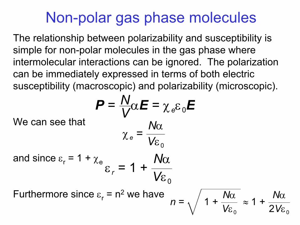
Non-polar gas phase moleculesThe relationship between polarizability and susceptibility issimple for non-polar molecules in the gas phase where intermolecular interactions can be ignored. The polarization can be immediately expressed in terms of both electric susceptibility (macroscopic) and polarizability (microscopic).

We can see that

and since εr = 1 + χe

Furthermore since εr = n2 we have

P = NVαE = χeε0E

χe =NαVε0

ε r = 1 +NαVε0

n = 1 +NαVε0

≈ 1 +Nα

2Vε0

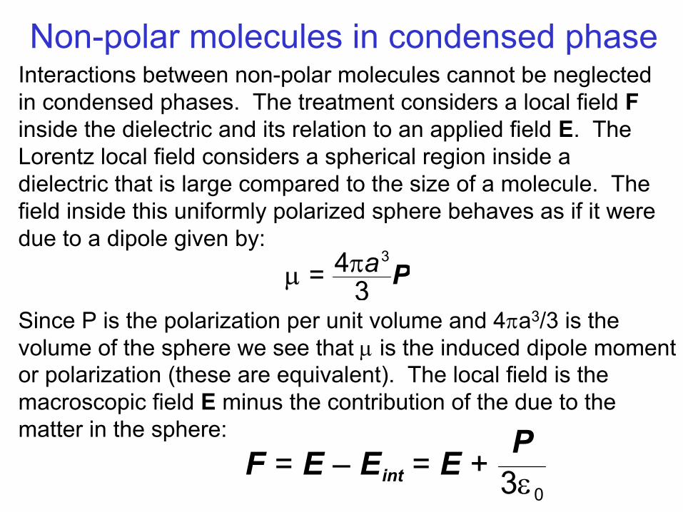
Non-polar molecules in condensed phaseInteractions between non-polar molecules cannot be neglected in condensed phases. The treatment considers a local field Finside the dielectric and its relation to an applied field E. The Lorentz local field considers a spherical region inside a dielectric that is large compared to the size of a molecule. The field inside this uniformly polarized sphere behaves as if it were due to a dipole given by:

Since P is the polarization per unit volume and 4πa3/3 is the volume of the sphere we see that µ is the induced dipole momentor polarization (these are equivalent). The local field is the macroscopic field E minus the contribution of the due to the matter in the sphere:

µ = 4πa3

3 P

F = E – Eint = E +P

3ε0

Lorentz local fieldSince

the Lorentz local field is

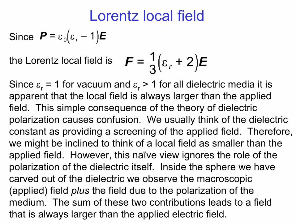
Since εr = 1 for vacuum and εr > 1 for all dielectric media it is apparent that the local field is always larger than the applied field. This simple consequence of the theory of dielectric polarization causes confusion. We usually think of the dielectric constant as providing a screening of the applied field. Therefore, we might be inclined to think of a local field as smaller than the applied field. However, this naïve view ignores the role of the polarization of the dielectric itself. Inside the sphere we have carved out of the dielectric we observe the macroscopic (applied) field plus the field due to the polarization of the medium. The sum of these two contributions leads to a field that is always larger than the applied electric field.

P = ε0 ε r – 1 E

F = 13 ε r + 2 E

The Clausius-Mosotti EquationThe polarization is the number density times the polarizability times the local field.

We eliminate E to obtain the Clausius-Mossotti equation.

This equation connects the macroscopic dielectric constant εrto the microscopic polarizability. Since εr = n2 we can replace these to obtain the Lorentz-Lorentz equation:

n2 – 1n2 + 2

= Nα3ε0V

ε r – 1ε r + 2 = Nα

3ε0V

P = NαV F = Nα

3V ε r + 2 E = ε0 ε r – 1 E

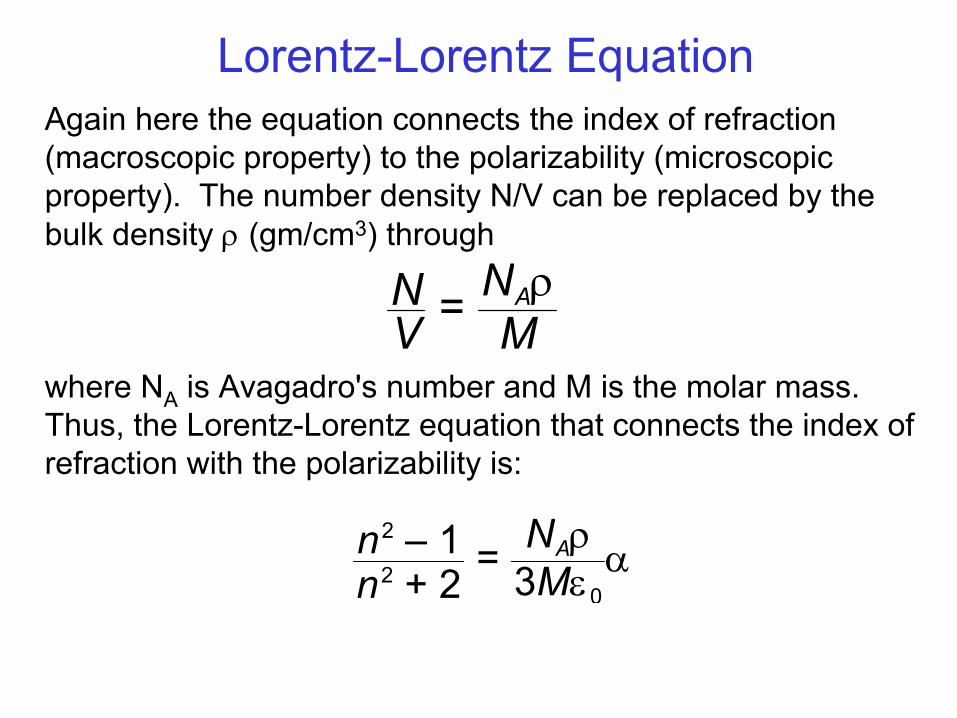
Lorentz-Lorentz EquationAgain here the equation connects the index of refraction (macroscopic property) to the polarizability (microscopic property). The number density N/V can be replaced by the bulk density ρ (gm/cm3) through

where NA is Avagadro's number and M is the molar mass.Thus, the Lorentz-Lorentz equation that connects the index ofrefraction with the polarizability is:

NV = NAρ

M

n2 – 1n2 + 2

= NAρ3Mε0

α

Polar moleculesThe polarization we have discussed up to now is the

electronic polarization. If a collection of non-polar molecules is subjected to an applied electric field the polarization is induced only in their electron distribution. However, if molecules in the collection possess a permanent ground state dipole moment, these molecules will tend to reorient in the applied field. The alignment of the dipoles will be disrupted by thermal motion that tends to randomize the orientation of the dipoles. The nuclear polarization will then be an equilibrium (or ensemble) average of dipoles aligned in the field.

P0 =N µV

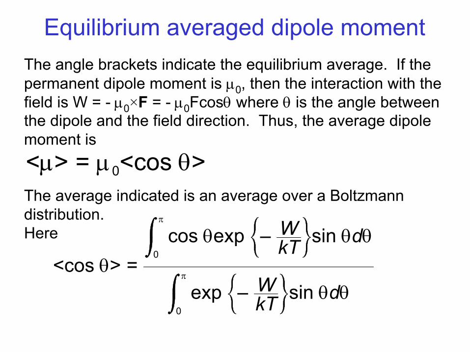
Equilibrium averaged dipole momentThe angle brackets indicate the equilibrium average. If the permanent dipole moment is µ0, then the interaction with the field is W = - µ0×F = - µ0Fcosθ where θ is the angle between the dipole and the field direction. Thus, the average dipole moment is

The average indicated is an average over a Boltzmann distribution.Here

<µ> = µ0<cos θ>

<cos θ> =cos θexp – WkT sin θdθ

0

π

exp – WkT sin θdθ0

π

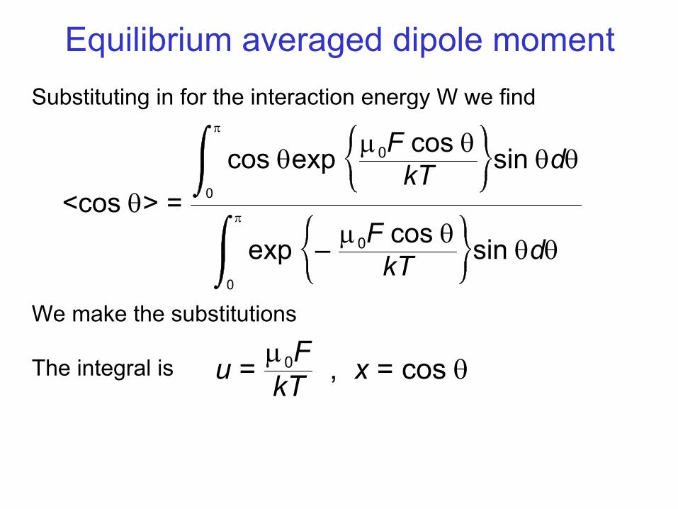
Equilibrium averaged dipole momentSubstituting in for the interaction energy W we find

We make the substitutions

The integral is

<cos θ> =cos θexp µ0F cos θ

kT sin θdθ0

π

exp – µ0F cos θkT sin θdθ

0

π

u = µ0FkT , x = cos θ

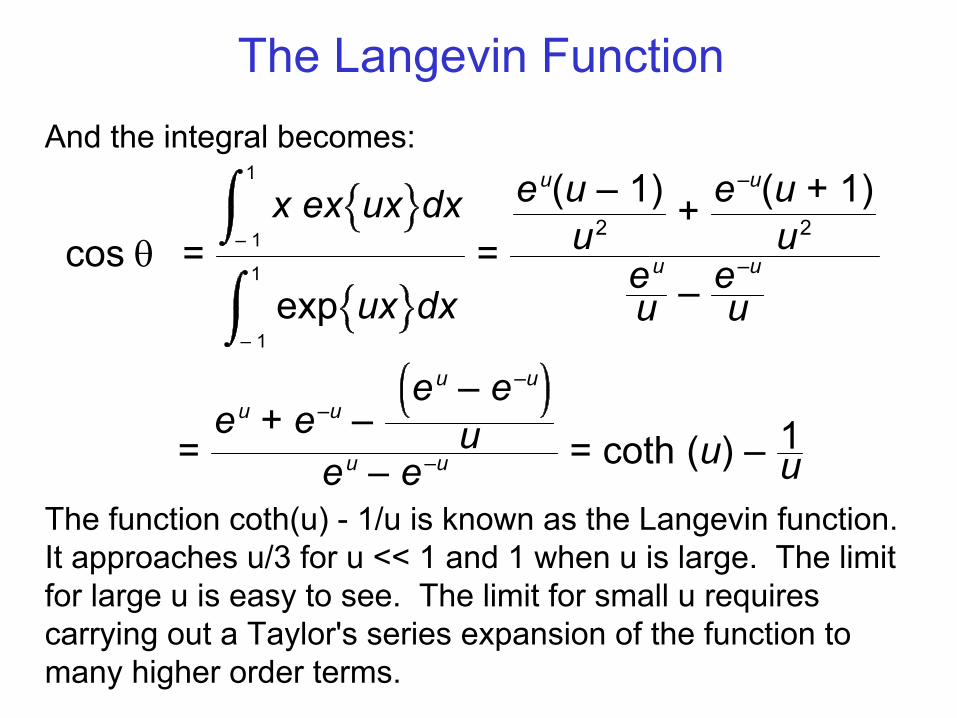
The Langevin FunctionAnd the integral becomes:

The function coth(u) - 1/u is known as the Langevin function. It approaches u/3 for u << 1 and 1 when u is large. The limit for large u is easy to see. The limit for small u requires carrying out a Taylor's series expansion of the function to many higher order terms.

cos θ =x ex ux dx

– 1

1

exp ux dx– 1

1=

eu(u – 1)u2 + e

–u(u + 1)u2

euu – e

–u

u

=eu + e–u –

eu – e–u

ueu – e–u = coth (u) – 1

u

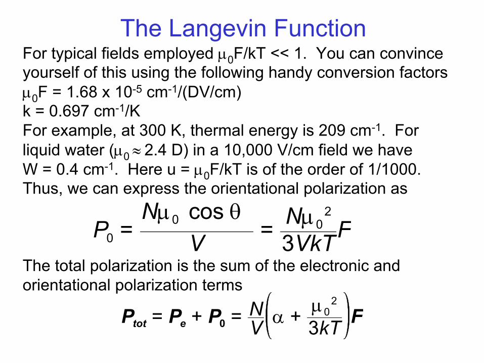
The Langevin FunctionFor typical fields employed µ0F/kT << 1. You can convince yourself of this using the following handy conversion factorsµ0F = 1.68 x 10-5 cm-1/(DV/cm)k = 0.697 cm-1/KFor example, at 300 K, thermal energy is 209 cm-1. For liquid water (µ0 ≈ 2.4 D) in a 10,000 V/cm field we have W = 0.4 cm-1. Here u = µ0F/kT is of the order of 1/1000.Thus, we can express the orientational polarization as

The total polarization is the sum of the electronic and orientational polarization terms

P0 =Nµ0 cos θ

V = Nµ02

3VkTF

Ptot = Pe + P0 = NV α + µ02

3kT F

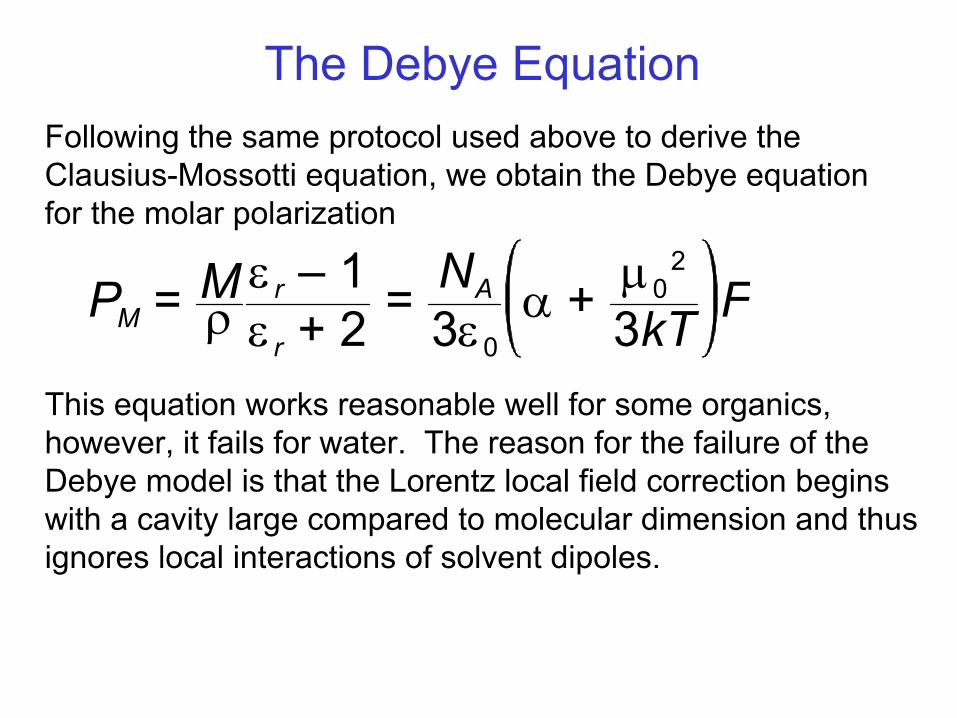
The Debye EquationFollowing the same protocol used above to derive the Clausius-Mossotti equation, we obtain the Debye equation for the molar polarization

This equation works reasonable well for some organics, however, it fails for water. The reason for the failure of the Debye model is that the Lorentz local field correction begins with a cavity large compared to molecular dimension and thus ignores local interactions of solvent dipoles.

PM = Mρε r – 1ε r + 2 = NA

3ε0α + µ0

2

3kT F

The Local Field ProblemThe local field problem is one of the most vexing problems of condensed phase electrostatics. Following Lorentz there are two models, the Onsager model and the Kirkwood model that attempt to account for the local interactions of solvent molecules in an applied electric field. The approaches discussed here are all continuum approaches in that there is a cavity and outside that cavity the medium is treated as a continuum dielectric with dielectric constant εr. The models differ in how they define the cavity. As stated above, Lorentz model assumes a large cavity (a is much larger than the molecule size). The Onsager model focuses on the creation of a cavity around a single molecule of interest (a is equal to the molecule size). The Kirkwood model includes a cluster around the molecule to account for local structure.

The Onsager ModelThe Debye model assumes that the dipole µ0 is not affected by the solvation shell. Yet consider water which has a gas phase dipole moment of 1.86 D and in condensed phase has a dipole moment in the range 2.3 - 2.4 D. The neighboring water molecules have a large effect inducing a dipole moment more than 25% larger than the gas phase dipole moment. The dipole moment m is the sum of the permanent and induced parts

The local field F has two contributions, the cavity field G and the reaction field R.

The cavity field is given the spherical cavity approximation in terms of the applied field

m = µ0 + αF

F = G +R

G = 3ε r2ε r + 1E

The Onsager ModelNotice that the cavity field is always greater than one. This is exactly analogous to the Lorentz local field. However, the Lorentz local field increases without bound as εr increases. The Onsager cavity field increases from 1 to 1.5 as εrapproaches ∞. The reaction field is proportional to the dipole moment of the molecule in the cavity:

The reaction field is always parallel to the permanent dipole moment. Only the cavity field can exert a torque on the dipole and cause it to align in the applied field. By separating these two effects the Onsager model improves upon the Debye equation..

R = ε r – 12ε r + 1

m2πa3ε0

≡ gm

The Onsager ModelThe Onsager reaction field is also an important relation for understanding the effect of solvents on the absorption and emission spectra of polar and polarizable molecules.Solvatochromism is the measurement of the effect of the solvent on the maximum position of the absorption band. Relaxation dynamics are also measured by determining the change in fluorescence maximum in fluorescent dyes in order to obtain an estimate of the reorientational dynamics of solvents.

Frequency dependent dielectric functionViewed from a microscopic perspective we know that the molecular polarizability is frequency dependent. Electronic polarizability is present in all molecules and has a response time that is rapid (> 1014 s-1). The high frequency response can follow the undulations of electromagnetic radiation in the visible region and hence this response gives rise to refraction of light. This contribution is the high frequency or optical dielectric constant, ε∞. There is a nuclear polarizability in polar molecules due to their tendency to align in an applied electric field due to the torque of the applied field in the frequency range from 106 to 1010 s-1. These motions give rise to absorption and dispersion in the microwave region. They also contribute to the low frequency or static dielectric constant, ε0. The static dielectric constant is not really static, but rather is due to changes in the electrical response due to dipolar reorientation.

Complex dielectric functionWe shall dissect the relative permittivity, εr into real and imaginary parts:

These two contributions represent the in-phase (εr') and out-of-phase (εr'') components of the frequency response of the medium. The in-phase component results in dispersion. Physically this means refraction of the electromagnetic radiation as it passes through the medium. The out-of-phase component gives rise to absorption. Absorption occurs in the visible (electronic state transitions), infrared (vibrational transitions), and microwave (rotational transitions). The real and imaginary parts of the frequency dependence dielectric response are related to one another by Kramers-Kronig relations.

ε r ω = ε r′ ω + iε r′′ ω

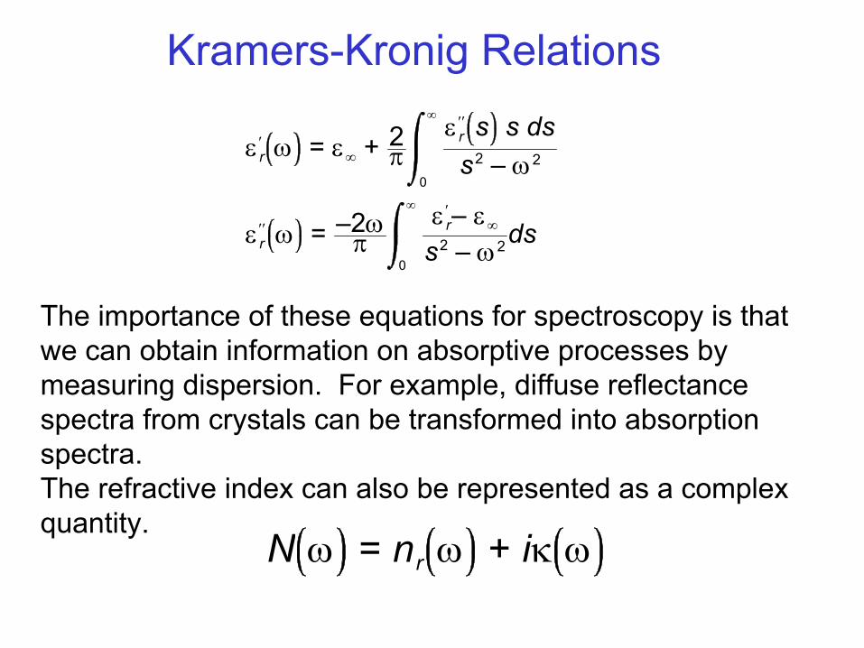
Kramers-Kronig Relations

The importance of these equations for spectroscopy is that we can obtain information on absorptive processes by measuring dispersion. For example, diffuse reflectance spectra from crystals can be transformed into absorption spectra. The refractive index can also be represented as a complex quantity.

ε r′ ω = ε∞ + 2π

ε r′′ s s dss2 – ω2

0

∞

ε r′′ ω = –2ωπ

ε r′– ε∞

s2 – ω2ds0

∞

N ω = nr ω + iκ ω

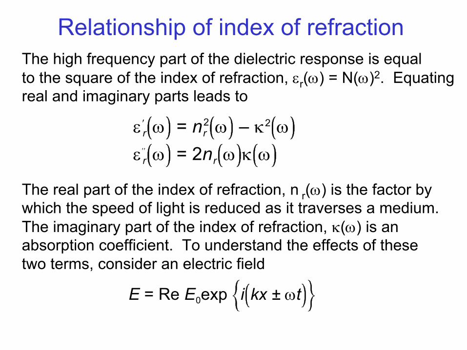
Relationship of index of refractionThe high frequency part of the dielectric response is equal to the square of the index of refraction, εr(ω) = N(ω)2. Equating real and imaginary parts leads to

The real part of the index of refraction, n r(ω) is the factor by which the speed of light is reduced as it traverses a medium. The imaginary part of the index of refraction, κ(ω) is an absorption coefficient. To understand the effects of these two terms, consider an electric field

ε r′ ω = nr2 ω – κ2 ωε r

′′ ω = 2nr ω κ ω

E = Re E0exp i kx ± ωt

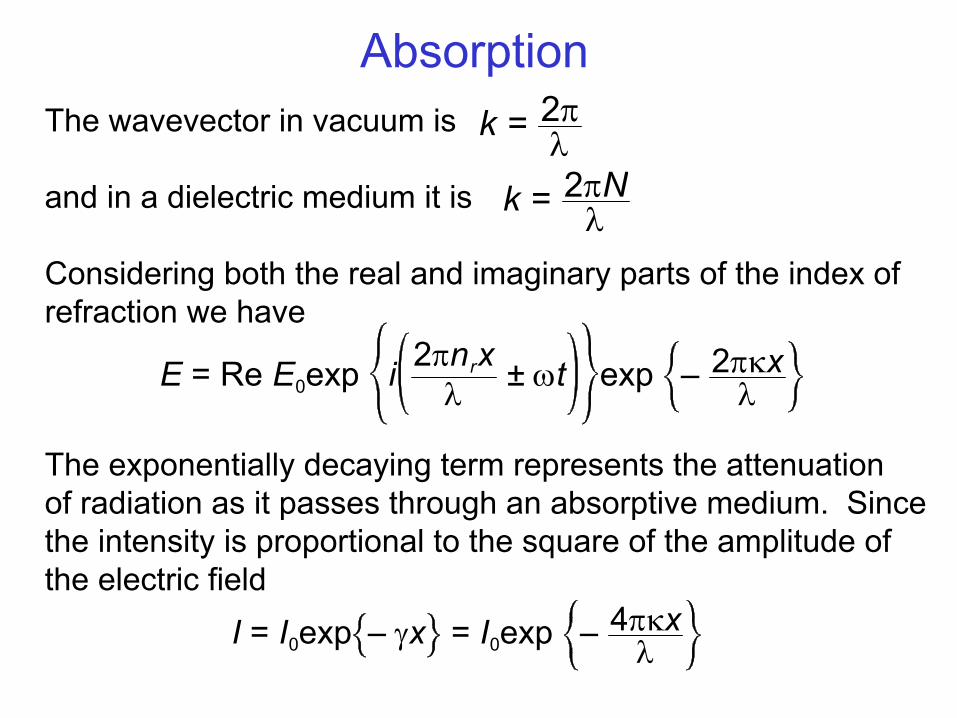
AbsorptionThe wavevector in vacuum is

and in a dielectric medium it is

Considering both the real and imaginary parts of the index of refraction we have

The exponentially decaying term represents the attenuation of radiation as it passes through an absorptive medium. Since the intensity is proportional to the square of the amplitude of the electric field

k = 2πλ

E = Re E0exp i 2πnrxλ ± ωt exp – 2πκx

λ

I = I0exp – γx = I0exp – 4πκxλ

k = 2πNλ

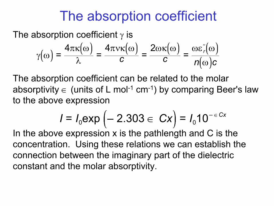
The absorption coefficientThe absorption coefficient γ is

The absorption coefficient can be related to the molar absorptivity ∈ (units of L mol-1 cm-1) by comparing Beer's law to the above expression

In the above expression x is the pathlength and C is the concentration. Using these relations we can establish the connection between the imaginary part of the dielectric constant and the molar absorptivity.

I = I0exp – 2.303 ∈ Cx = I010– ∈Cx

γ ω =4πκ ω

λ =4πνκ ω

c =2ωκ ωc =

ωε r′′ ωn ω c

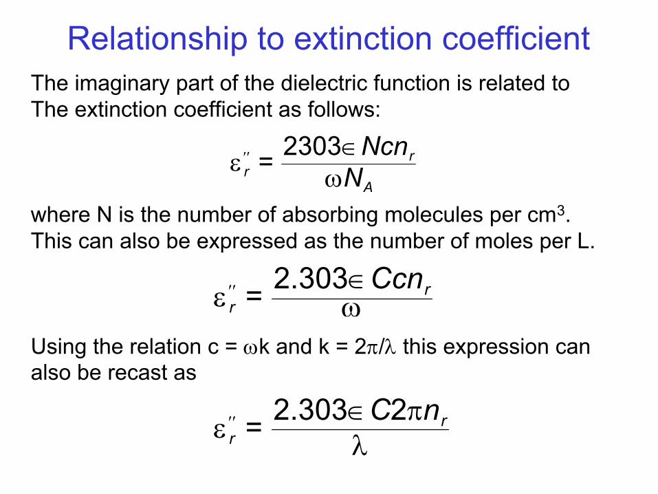
Relationship to extinction coefficientThe imaginary part of the dielectric function is related toThe extinction coefficient as follows:

where N is the number of absorbing molecules per cm3. This can also be expressed as the number of moles per L.

Using the relation c = ωk and k = 2π/λ this expression can also be recast as

ε r′′ = 2303∈NcnrωNA

ε r′′ = 2.303∈Ccnrω

ε r′′ = 2.303∈C2πnrλ