Embed Size (px)
Citation preview
Advanced Quantum Mechanics
Geert BrocksFaculty of Applied Physics, University of Twente
August 2002

ii
Contents
Preface xiii
I Single Particles 1
1 Quantum Mechanics 3
1.1 Wave Mechanics . . . . . . . . . . . . . . . . . . . . . . . . . . . . . . . . . 3
1.2 Quantum Mechanics . . . . . . . . . . . . . . . . . . . . . . . . . . . . . . . 7
1.3 Representations . . . . . . . . . . . . . . . . . . . . . . . . . . . . . . . . . . 8
1.3.1 General Formalism . . . . . . . . . . . . . . . . . . . . . . . . . . . . 8
1.3.2 The Position Representation; Wave Mechanics Revisited . . . . . . . 9
1.4 Many Particles and Product States . . . . . . . . . . . . . . . . . . . . . . . 13
2 Time Dependent Perturbation Theory 17
2.1 Time Evolution . . . . . . . . . . . . . . . . . . . . . . . . . . . . . . . . . . 17
2.1.1 The Huygens Principle . . . . . . . . . . . . . . . . . . . . . . . . . . 19
2.2 Time Dependent Perturbations . . . . . . . . . . . . . . . . . . . . . . . . . 21
2.3 Fermi’s Golden Rule . . . . . . . . . . . . . . . . . . . . . . . . . . . . . . . 23
2.4 Radiative Transitions . . . . . . . . . . . . . . . . . . . . . . . . . . . . . . . 30
2.4.1 Atom in a Radiation Field . . . . . . . . . . . . . . . . . . . . . . . . 30
2.4.2 Einstein Coefficients and Rate Equations . . . . . . . . . . . . . . . 32
2.4.3 Population and Lifetime . . . . . . . . . . . . . . . . . . . . . . . . . 35
2.5 Epilogue . . . . . . . . . . . . . . . . . . . . . . . . . . . . . . . . . . . . . . 36
2.6 Appendix I. The Heisenberg Picture . . . . . . . . . . . . . . . . . . . . . . 37
2.7 Appendix II. Some Integral Tricks . . . . . . . . . . . . . . . . . . . . . . . 40
3 The Quantum Pinball Game 43
3.1 A Typical Experiment . . . . . . . . . . . . . . . . . . . . . . . . . . . . . . 43
3.2 Time Evolution; Summing the Perturbation Series . . . . . . . . . . . . . . 45
3.2.1 Adapt Integration Bounds; Green Functions . . . . . . . . . . . . . . 47
3.2.2 Fourier Transform to the Frequency Domain . . . . . . . . . . . . . 49
3.2.3 Sum the Perturbation Series; Dyson Equation . . . . . . . . . . . . . 50
3.2.4 Green Functions; Closed Expressions . . . . . . . . . . . . . . . . . . 51
3.2.5 Summary . . . . . . . . . . . . . . . . . . . . . . . . . . . . . . . . . 53
3.3 Connection to Mattuck’s Ch. 3 . . . . . . . . . . . . . . . . . . . . . . . . . 54
3.4 Appendix. Green Functions; the Lippmann-Schwinger Equation . . . . . . . 55
3.4.1 The Huygens Principle Revisited . . . . . . . . . . . . . . . . . . . . 59
iii
iv CONTENTS
4 Scattering 614.1 Scattering by a Dilute Concentration of Centers . . . . . . . . . . . . . . . . 62
4.1.1 The Scattering Cross Section . . . . . . . . . . . . . . . . . . . . . . 654.1.2 Forward Scattering; the Optical Theorem . . . . . . . . . . . . . . . 67
4.2 Scattering by a Single Center . . . . . . . . . . . . . . . . . . . . . . . . . . 694.3 Re-summation of the Series; the Self-Energy . . . . . . . . . . . . . . . . . 724.4 The Physical Meaning of Self-Energy . . . . . . . . . . . . . . . . . . . . . . 744.5 The Scattering Cross Section . . . . . . . . . . . . . . . . . . . . . . . . . . 77
4.5.1 The Lippmann-Schwinger Equation . . . . . . . . . . . . . . . . . . 774.5.2 The Scattering Amplitudes and the Differential Cross Section . . . . 824.5.3 The Born Series and the Born approximation . . . . . . . . . . 83
4.6 Epilogue . . . . . . . . . . . . . . . . . . . . . . . . . . . . . . . . . . . 854.7 Appendix I. The Refractive Index . . . . . . . . . . . . . . . . . . . . . . . . 854.8 Appendix II. Applied Complex Function Theory . . . . . . . . . . . . . . . 87
4.8.1 Complex Integrals; the Residue Theorem . . . . . . . . . . . . . . . 874.8.2 Contour Integration . . . . . . . . . . . . . . . . . . . . . . . . . . . 894.8.3 The Principal Value . . . . . . . . . . . . . . . . . . . . . . . . . . . 924.8.4 The Self-Energy Integral . . . . . . . . . . . . . . . . . . . . . . . . . 94
II Many Particles 97
5 Quantum Field Oscillators 995.1 The Quantum Oscillator . . . . . . . . . . . . . . . . . . . . . . . . . . . . . 99
5.1.1 Summary Harmonic Oscillator . . . . . . . . . . . . . . . . . . . . . 1025.1.2 Second Quantization . . . . . . . . . . . . . . . . . . . . . . . . . . . 103
5.2 The One-dimensional Quantum Chain; Phonons . . . . . . . . . . . . . . . 1045.3 My First Quantum Field . . . . . . . . . . . . . . . . . . . . . . . . . . . . . 108
5.3.1 Classical Chain . . . . . . . . . . . . . . . . . . . . . . . . . . . . . . 1095.3.2 Continuum Limit: an Elastic Medium . . . . . . . . . . . . . . . . . 1105.3.3 Quantizing the Elastic Medium; Phonons . . . . . . . . . . . . . . . 113
5.4 The Three-dimensional Quantum Chain . . . . . . . . . . . . . . . . . . . . 1155.4.1 Discrete Lattice . . . . . . . . . . . . . . . . . . . . . . . . . . . . . . 1155.4.2 Elastic Medium . . . . . . . . . . . . . . . . . . . . . . . . . . . . . . 1165.4.3 Are Phonons Real Particles ? . . . . . . . . . . . . . . . . . . . . . 117
5.5 The Electro-Magnetic Field in Vacuum . . . . . . . . . . . . . . . . . . . . . 1185.5.1 Classical Electro-Dynamics . . . . . . . . . . . . . . . . . . . . . . . 1195.5.2 Quantum Electro-Dynamics (QED) . . . . . . . . . . . . . . . . . . 1215.5.3 Are Photons Real Particles ? . . . . . . . . . . . . . . . . . . . . . . 124
6 Bosons and Fermions 1276.1 N particles; the Stone Age . . . . . . . . . . . . . . . . . . . . . . . . . . . . 127
6.1.1 The Slater Determinant . . . . . . . . . . . . . . . . . . . . . . . . . 1316.1.2 Three Particle Example Work-out . . . . . . . . . . . . . . . . . . . 1326.1.3 One- and Two-particle Operators . . . . . . . . . . . . . . . . . . . . 133
6.2 N particles; the Modern Era . . . . . . . . . . . . . . . . . . . . . . . . . . 1346.2.1 Second Quantization for Bosons . . . . . . . . . . . . . . . . . . . . 1346.2.2 Second Quantization for Fermions . . . . . . . . . . . . . . . . . . . 137
CONTENTS v
6.2.3 The Road Travelled . . . . . . . . . . . . . . . . . . . . . . . . . . . 1416.3 The Particle-Hole Formalism . . . . . . . . . . . . . . . . . . . . . . . . . . 143
6.3.1 The Homogeneous Electron Gas . . . . . . . . . . . . . . . . . . . . 1436.3.2 Particles and Holes . . . . . . . . . . . . . . . . . . . . . . . . . . . . 1456.3.3 The Quantum Field Theory Connection . . . . . . . . . . . . . . . . 149
6.4 Second Quantization and the Electron Field . . . . . . . . . . . . . . . . . . 1506.5 Appendix I. Identical Particle Algebra . . . . . . . . . . . . . . . . . . . . . 154
6.5.1 Normalization Factors and Orthogonality . . . . . . . . . . . . . . . 1546.5.2 Second Quantization for Operators . . . . . . . . . . . . . . . . . . . 156
6.6 Appendix II. Identical Particles . . . . . . . . . . . . . . . . . . . . . . . . 1626.6.1 Indistinguishable Particles . . . . . . . . . . . . . . . . . . . . . . . . 1626.6.2 Why Symmetrize ? . . . . . . . . . . . . . . . . . . . . . . . . 1636.6.3 Symmetrize The Universe ? . . . . . . . . . . . . . . . . . . . . . . . 165
7 Optics 1697.1 Atoms and Radiation; the Full Monty . . . . . . . . . . . . . . . . . . . . . 169
7.1.1 Absorption; Fermi’s Golden Rule . . . . . . . . . . . . . . . . . . . . 1737.1.2 Spontaneous Emission . . . . . . . . . . . . . . . . . . . . . . . . . . 175
7.2 Electrons, Holes and Photons . . . . . . . . . . . . . . . . . . . . . . . . . . 1767.2.1 Electrons and Radiation . . . . . . . . . . . . . . . . . . . . . . . . . 1777.2.2 Free Electrons and Holes . . . . . . . . . . . . . . . . . . . . . . . . 1797.2.3 Light Absorption by Electrons and Holes . . . . . . . . . . . . . . . 1827.2.4 Light Scattering by Free Electrons . . . . . . . . . . . . . . . . . . . 187
7.3 Higher Order Processes; the Quantum Pinball Game . . . . . . . . . . 1887.4 Appendix I. Interaction of an Electron with an EM field . . . . . . . . . . . 190
7.4.1 Dipole Approximation . . . . . . . . . . . . . . . . . . . . . . . . . 1927.5 Appendix II. Relativistic Electrons and Holes . . . . . . . . . . . . . . . . . 193
III Interacting Particles 199
8 Propagators and Diagrams 2018.1 The Single Particle Propagator . . . . . . . . . . . . . . . . . . . . . . . . . 202
8.1.1 A Gedanken Experiment . . . . . . . . . . . . . . . . . . . . . . . . . 2038.1.2 Particle and Hole Propagators . . . . . . . . . . . . . . . . . . . . . 204
8.2 A Single Particle or Hole . . . . . . . . . . . . . . . . . . . . . . . . . . . . . 2058.2.1 Particle Scattering . . . . . . . . . . . . . . . . . . . . . . . . . . . . 2058.2.2 The Second Quantization Connection . . . . . . . . . . . . . . . . . 2078.2.3 Hole Scattering . . . . . . . . . . . . . . . . . . . . . . . . . . . . 209
8.3 Many Particles and Holes . . . . . . . . . . . . . . . . . . . . . . . . . . . . 2118.3.1 Atom Embedded in an Electron Gas . . . . . . . . . . . . . . . . . . 2148.3.2 Goldstone Diagrams; Exchange . . . . . . . . . . . . . . . . . . . . . 2158.3.3 Diagram Expansion . . . . . . . . . . . . . . . . . . . . . . . . . . . 2188.3.4 Diagram Summation . . . . . . . . . . . . . . . . . . . . . . . . . . . 2198.3.5 Exponential Decay . . . . . . . . . . . . . . . . . . . . . . . . . . . 222
8.4 Interacting Particles and Holes . . . . . . . . . . . . . . . . . . . . . . . . . 2238.4.1 Two-Particle Diagrams . . . . . . . . . . . . . . . . . . . . . . . . . 2258.4.2 The Homogeneous Electron Gas Revisited . . . . . . . . . . . . . . . 227
vi CONTENTS
8.4.3 The Full Diagram Dictionary . . . . . . . . . . . . . . . . . . . . 2288.4.4 Radiation Diagrams . . . . . . . . . . . . . . . . . . . . . . . . . . . 229
8.5 The Spectral Function . . . . . . . . . . . . . . . . . . . . . . . . . . . . . . 2308.5.1 Physical Content . . . . . . . . . . . . . . . . . . . . . . . . . . . . . 232
8.6 (Inverse) Photoemission and Quasi-particles . . . . . . . . . . . . . . . . . 2338.6.1 Photoemission . . . . . . . . . . . . . . . . . . . . . . . . . . . . . . 2338.6.2 Inverse Photoemission . . . . . . . . . . . . . . . . . . . . . . . . . . 235
8.7 Appendix I. The Adiabatic Connection . . . . . . . . . . . . . . . . . . . . . 2378.7.1 The Problem . . . . . . . . . . . . . . . . . . . . . . . . . . . . . . . 2378.7.2 The Solution . . . . . . . . . . . . . . . . . . . . . . . . . . . . . . . 238
8.8 Appendix II. The Linked Cluster Expansion . . . . . . . . . . . . . . . . . . 2418.8.1 Denominator . . . . . . . . . . . . . . . . . . . . . . . . . . . . . 2428.8.2 Numerator . . . . . . . . . . . . . . . . . . . . . . . . . . . . . . . . 2458.8.3 Linked Cluster Theorem . . . . . . . . . . . . . . . . . . . . . . . . . 250
9 The electron-electron interaction 2539.1 Many interacting electrons . . . . . . . . . . . . . . . . . . . . . . . . . . . . 2539.2 The Hartree approximation . . . . . . . . . . . . . . . . . . . . . . . . . . . 255
9.2.1 The Hartree (Coulomb) interaction . . . . . . . . . . . . . . . . . . . 2569.2.2 The Hartree Self-Consistent Field equations . . . . . . . . . . . . . . 2609.2.3 Pro’s and con’s of the Hartree approximation . . . . . . . . . . . . . 265
9.3 The Hartree-Fock approximation . . . . . . . . . . . . . . . . . . . . . . . . 2669.3.1 The exchange interaction . . . . . . . . . . . . . . . . . . . . . . . . 2679.3.2 The Hartree-Fock Self-Consistent Field equations . . . . . . . . . . . 2719.3.3 The homogeneous electron gas revisited . . . . . . . . . . . . . . . . 2749.3.4 Pro’s and con’s of the Hartree-Fock approximation . . . . . . . . . . 2809.3.5 Screening . . . . . . . . . . . . . . . . . . . . . . . . . . . . . . . . . 282
9.4 The Random Phase Approximation (RPA) . . . . . . . . . . . . . . . . . . 2839.4.1 The RPA diagram . . . . . . . . . . . . . . . . . . . . . . . . . . . 2849.4.2 The RPA screened interaction . . . . . . . . . . . . . . . . . . . . . . 2879.4.3 The GW approximation . . . . . . . . . . . . . . . . . . . . . . . . . 2909.4.4 The homogeneous electron gas re-revisited . . . . . . . . . . . . . . . 293
List of Figures
2.1 Progagation of a wave using the Huygens principle. . . . . . . . . . . . . . . 20
2.2 Feynman diagram. . . . . . . . . . . . . . . . . . . . . . . . . . . . . . . . . 23
2.3 Dictionary of Feynman diagrams. . . . . . . . . . . . . . . . . . . . . . . . . 23
2.4 The Born approximation in Feynman diagrams. . . . . . . . . . . . . . . . . 24
2.5 Typical line-shape function F (ω). . . . . . . . . . . . . . . . . . . . . . . . 29
2.6 Optical processes involving the levels i and f ; Einstein A,B coefficients. . . 32
2.7 Radiative processes. . . . . . . . . . . . . . . . . . . . . . . . . . . . . . . . 34
2.8 The function 4T (ω) . . . . . . . . . . . . . . . . . . . . . . . . . . . . . . . 41
3.1 Typical quantum experiment. . . . . . . . . . . . . . . . . . . . . . . . . . . 44
3.2 Feynman diagram of the absorption of a photon. . . . . . . . . . . . . . . . 45
3.3 A ‘physical’ theta function. . . . . . . . . . . . . . . . . . . . . . . . . . . . 51
3.4 Propagation of a wave using the Huygens principle. . . . . . . . . . . . . . . 59
4.1 Scattering of a single particle by a fixed target. . . . . . . . . . . . . . . . . 62
4.2 Incoherent scattering of wave packets in a dilute sample. . . . . . . . . . . . 64
4.3 Scattering geometry. . . . . . . . . . . . . . . . . . . . . . . . . . . . . . . . 66
4.4 Perturbation series for single particle scattering. . . . . . . . . . . . . . . . 71
4.5 Perturbation series rewritten in terms of self energy. . . . . . . . . . . . . . 72
4.6 the self energy for single particle scattering . . . . . . . . . . . . . . . . . . 72
4.7 Angle resolved scattering detection. . . . . . . . . . . . . . . . . . . . . . . . 78
4.8 Adding layers to calculate the index of refraction. . . . . . . . . . . . . . . . 86
4.9 Contour integration = integration along a path in the complex plane. . . . 87
4.10 A closed contour C in the complex plane. . . . . . . . . . . . . . . . . . . . 88
4.11 Cauchy’s integral formula. . . . . . . . . . . . . . . . . . . . . . . . . . . . . 88
4.12 Closing the contour in the lower half plane. . . . . . . . . . . . . . . . . . . 90
4.13 Closing the contour in the upper half plane. . . . . . . . . . . . . . . . . . . 91
4.14 Lorenzian line shape function. . . . . . . . . . . . . . . . . . . . . . . . . . . 93
5.1 A linear chain of masses and springs. . . . . . . . . . . . . . . . . . . . . . 104
5.2 Dispersion relation of a linear chain ω (k) = 2p
κm | sin 12ka|. . . . . . . . . . 107
5.3 An elastic medium with displacements u at points xm (top figure). Artist’simpression of continuum (bottom figure). . . . . . . . . . . . . . . . . . . . 109
5.4 Scattering of a neutron and emission (left) or absorption (right) of a phonon.118
5.5 Compton scattering of X-rays. . . . . . . . . . . . . . . . . . . . . . . . . . . 125
6.1 An N -boson state. . . . . . . . . . . . . . . . . . . . . . . . . . . . . . . . . 134
6.2 An N -fermion state. . . . . . . . . . . . . . . . . . . . . . . . . . . . . . . . 138
vii
viii LIST OF FIGURES
6.3 Absorption of a photon. . . . . . . . . . . . . . . . . . . . . . . . . . . . . . 142
6.4 Shells of constant ²k. . . . . . . . . . . . . . . . . . . . . . . . . . . . . . . 145
6.5 Particle and hole energies relative to the Fermi level. . . . . . . . . . . . . . 149
6.6 Two particles in two separated wave packets. . . . . . . . . . . . . . . . . . 163
6.7 Two particles in overlapping wave packets. . . . . . . . . . . . . . . . . . . . 165
7.1 Absorption of a photon by an electron. . . . . . . . . . . . . . . . . . . . . . 179
7.2 Absorption of a photon by an electron. . . . . . . . . . . . . . . . . . . . . . 180
7.3 Absorption of a photon, creating an electron-hole pair. . . . . . . . . . . . . 182
7.4 Creation of a particle-hole pair by a photon. . . . . . . . . . . . . . . . . . . 184
7.5 Creation of a particle-hole pair by a photon. . . . . . . . . . . . . . . . . . . 185
7.6 Absorption of a photon by a bound hole. . . . . . . . . . . . . . . . . . . . . 186
7.7 Annihilation of a particle-hole pair creates a photon. . . . . . . . . . . . . . 186
7.8 A contribution to electron-photon (or Compton) scattering. . . . . . . . . . 187
7.9 An 8th order electron-electron scattering diagram. . . . . . . . . . . . . . . 189
7.10 Creation of a particle-hole pair; (a) non-relativistic, (b) relativistic. . . . . . 194
7.11 Relativistic particle-hole spectrum. . . . . . . . . . . . . . . . . . . . . . . . 195
7.12 Energy-momentum dispersion relations of an electron (top thick curve), ahole (bottom thick curve), and a photon (thin straight line). . . . . . . . . . 196
7.13 Cascade induced by a high energy electron. . . . . . . . . . . . . . . . . . . 197
8.1 A visual interpretation of the propagator i~G+(l,k,t1 − t0). . . . . . . . . . 2048.2 Second order potential scattering of a particle. . . . . . . . . . . . . . . . . 208
8.3 Second order potential scattering of a hole. . . . . . . . . . . . . . . . . . . 210
8.4 Mattuck’s table 4.2, p.75 . . . . . . . . . . . . . . . . . . . . . . . . . . . . . 211
8.5 Mattuck’s table 4.3, p.86. . . . . . . . . . . . . . . . . . . . . . . . . . . . . 229
8.6 Photoemission: incoming photon of energy ~ω and outgoing electron ofenergy ²q. . . . . . . . . . . . . . . . . . . . . . . . . . . . . . . . . . . . . . 233
8.7 Inverse photoemission: incoming electron of energy ² and outgoing photonof energy ~ωq. . . . . . . . . . . . . . . . . . . . . . . . . . . . . . . . . . . 236
9.1 The Hartree diagram . . . . . . . . . . . . . . . . . . . . . . . . . . . . . . . 257
9.2 Summing over Hartree diagrams . . . . . . . . . . . . . . . . . . . . . . . . 258
9.3 The self-consistent Hartree approximation . . . . . . . . . . . . . . . . . . . 264
9.4 The dressed (self-consistent) Hartree potential . . . . . . . . . . . . . . . . . 265
9.5 The exchange potential . . . . . . . . . . . . . . . . . . . . . . . . . . . . . 268
9.6 The exchange potential . . . . . . . . . . . . . . . . . . . . . . . . . . . . . 269
9.7 The exchange diagram . . . . . . . . . . . . . . . . . . . . . . . . . . . . . . 269
9.8 A fourth order Hartree-Fock diagram . . . . . . . . . . . . . . . . . . . . . . 270
9.9 Fourth order Hartree-Fock diagram . . . . . . . . . . . . . . . . . . . . . . . 270
9.10 The Hartee-Fock approximation . . . . . . . . . . . . . . . . . . . . . . . . . 273
9.11 The self-consistent (dressed) Hartree-Fock potential. . . . . . . . . . . . . . 274
9.12 Exchange energy as function of kkF
. . . . . . . . . . . . . . . . . . . . . . . 277
9.13 Hartree-Fock energies ²k and kinetic energies ²0,k for kF = 1a−10 . . . . . . . 278
9.14 ρX(r) =12π2
j1(r)r as function of r . . . . . . . . . . . . . . . . . . . . . . . . 279
9.15 ²0(k) = d²dk in the Hartree-Fock approximation. . . . . . . . . . . . . . . . . . 282
9.16 An eighth order RPA + Hartree-Fock diagram. . . . . . . . . . . . . . . . . 285
LIST OF FIGURES ix
9.17 The RPA approximation . . . . . . . . . . . . . . . . . . . . . . . . . . . . . 2869.18 The RPA or GW approximation . . . . . . . . . . . . . . . . . . . . . . . . 2909.19 The self-energy according to Thomas-Fermi screening . . . . . . . . . . . . 3009.20 The RPA quasi-particle energies using Thomas-Fermi screening . . . . . . . 3019.21 k-derivative of the HF (upper) and RPA/Thomas-Fermi (lower) particle
energies . . . . . . . . . . . . . . . . . . . . . . . . . . . . . . . . . . . . . . 3029.22 Quasi-particle energies as calculated within RPA. . . . . . . . . . . . . . . . 3049.23 The factor |ImΣX,RPA(k,k,ωk)| which determines the inverse quasi-particle
lifetime, in units of ²F , in the RPA approximation (lower curve). . . . . . . 3059.24 The weight factor zk at the Fermi level, |k| = kF as a function of rs . . . . 306

x LIST OF FIGURES
List of Tables
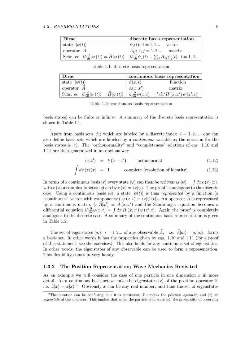
1.1 discrete basis representation . . . . . . . . . . . . . . . . . . . . . . . . . . . 91.2 continuous basis representation . . . . . . . . . . . . . . . . . . . . . . . . . 9
5.1 Comparison between a discrete classical chain and an elastic medium . . . . 113
6.1 Equation roadmap from 1st to 2nd quantization . . . . . . . . . . . . . . . . 1426.2 Particles and holes . . . . . . . . . . . . . . . . . . . . . . . . . . . . . . . . 148
xi

xii LIST OF TABLES
Preface
“The labour we delight in physics pain”, Shakespeare, Macbeth.1
This manuscript contains the lecture notes of the course “voortgezette quantum me-chanica” (advanced quantum mechanics). The course is intended for physics students earn-ing their master degree (4th/5th year) who are interested in modern theoretical physics.It is meant to form a bridge between elementary courses in quantum mechanics and themore advanced topical quantum mechanics books. Rather than reviewing all the topics ofan introductory course once again on a deeper level, I have chosen to make the quantummechanics of many-particle systems one of the main themes in this course. The emphasis ison general methods and interpretations—often borrowed from quantum field theory—, suchas second quantization and quasi-particles. Our main tool is time-dependent perturba-tion theory, which can be represented graphically by Feynman65 diagrams in a physicallyintuitive way.2 Model systems such as the electron gas and the elastic medium are usedto introduce the general structure of the physics, examples of relevant applications aremainly taken from condensed matter physics and optics. The organization of these notesis as follows. Part I introduces some of the basic tools of quantum mechanics, in par-ticular time-dependent perturbation theory. Part II describes some of the basic conceptsof many-fermion and -boson physics, (anti)particles, quasi-particles, second quantizationand quantum fields. Part III contains an introduction to more advanced topics, such aspropagators and diagrammatic expansions.
I have tried to make these notes self-contained with as few phrases such as “A littlealgebra yields ...” or “It can be shown that ... ” as possible. Such sentences alwaysannoyed me when I was a student; either show how it works, or leave the subject alone.Preparing these notes as a lecturer however I discovered that there is probably a good rea-son for such phrases. Without them, the text easily assumes the shape of an “omgevallenboekenkast”. I have tried to bring some order in this pile by presenting the more basicmaterial in the first sections of each chapter, collecting the more special (but often veryinteresting) topics in the final sections, and shifting some detailed algebra and backgroundmaterial to appendices. Topics such as scattering theory or quantum electro-dynamics areonly discussed superficially, since a thorough discussion would require too much space.Other topics, such as relativistic quantum mechanics or symmetry (group theory), areonly touched upon. They are more suitable for a specialized course. I stayed away from
1“It is a good thing for an uneducated man to read books of quotations”, Winston Churchill, My EarlyLife.
2The contributors to quantum theory and many-particle physics (or quantum field theory) make up alist of “who-is-who” in physics. I will mark Nobel prize winners by the year in which they recieved theiraward.
xiii
xiv PREFACE
the finite temperature formalism, since that is too difficult for me; in all the materialpresented here T = 0 is assumed.
I would like to thank Els Braker-Peerik for word-processing the first version of thesenotes from my hand-written papers. Also I wish to acknowledge Jeroen Hegeman for point-ing out an error in the original notes, which resulted from my urge to take a shortcut. More-over, I did my best to remove inconsistencies in notation, units and phase/normalizationfactors which plagued the original notes. At least the errors are more consistent now; ifyou spot any, please let me know.
A good working knowledge of elementary quantum mechanics is assumed, as wellas a knowledge of the basic mathematical tools of analysis, linear algebra and Fouriertransforms. Knowledge of complex function theory is useful, but not absolutely essential.The book you used in your introductory course is still helpful: D. J. Griffiths, Introductionto Quantum Mechanics, (Prentice Hall, New Jersey, 1995) . Although the present notesare reasonably self-contained, it is useful to have the following book; R. Mattuck, AnIntroduction to Feynman Diagrams in Many Particle Physics, (Dover, New York, 1992).I will make comparisons to the relevant passages of this book in these lecture notes. In(numerous) footnotes references are given to additional literature, if you are interested.
In the lecture notes I mainly discuss the general structure of the theory. Lecture notesare designed to make the lecturer superfluous. This is not so for the assignments whichare handed out each week. These are an integral part of this course. These exercises arevital in order to get familiarized with the theory. Moreover, they contain applications tophysical problems.
Part I
Single Particles
1

Chapter 1
Quantum Mechanics
“Though this be madness, yet there is method in it”, Shakespeare, Hamlet.
This chapter starts by summarizing the basic postulates of (Schrodinger33’s) wave me-chanics, which is the usual subject of introductory courses on quantum mechanics. Thesepostulates are actually applicable in a wider sense, which has lead Dirac33 to formulatethe structure of quantum mechanics in a more general way. Wave mechanics is only a spe-cific representation of quantum mechanics. The term “representation” has a well-definedmathematical meaning here, which is explained next in this chapter. Finally, it is shownhow to systematically construct quantum states for many particles and many degrees offreedom. This last section might only be glanced through at first reading; we will comeback to it at a later stage.
1.1 Wave Mechanics
Experiments and theoretical analysis have resulted in a number of postulates (or laws)upon which quantum mechanics is founded. They describe (1) how microscopic particlesmust be represented, (2) how to obtain quantities that can be observed, (3) how timeevolution must be described and (4) what the logical structure of (a series of) measure-ments is. The form of quantum mechanics you are probably most familiar with, is wavemechanics (or Schrodinger’s quantum mechanics as it is called in Appendix A of Mattuck).For a single particle the postulates of wave mechanics are summarized below. Mind you,the summary is very compact, and you should consult your introductory books, such asGriffiths, for more detail. If you find quantum mechanics strange, let me quote RichardFeynman65: “...the way we have to describe Nature is generally incomprehensible to us.”.In other words we don’t know why the physical postulates or laws are as they are, butthey are highly successful in explaining the phenomena, which is ultimately what countsin physics. The same probably holds for classical mechanics or electrodynamics as well;we just seem to be more familiar with Newton’s or Maxwell’s laws.
POSTULATES (single particle):
1. A particle is represented by a complex wave function ψ(r, t) where r = x, y, z is apoint in space and t is the time. Noteworthy properties are:
3
4 CHAPTER 1. QUANTUM MECHANICS
(a) If ψ(r, t) is an acceptable wave function and φ(r, t) is an acceptable wave func-tion, then aψ(r, t) + bφ(r, t) must also be an acceptable wave function, wherea, b are complex numbers. This is the superposition principle. Wave functionsthus form a linear vector space. In physical terms, the superposition principledescribes the phenomenon of interference of waves.
(b) The wave function itself is not directly observable; however the probability P (r)of finding the particle inside a small volume dV around the point r is given bythe intensity of the wave
P (r) =1
Nψ|ψ(r, t)|2 dV (1.1)
where the constant Nψ =R |ψ(r, t)|2 dV is chosen such that
RP (r)dV = 1;
(i.e., the particle has to be somewhere).
Only wave functions for which Nψ can be calculated as a finite number areacceptable. Defining the norm of a wave function as
pNψ, acceptable wave
functions thus have a finite norm.
(c) If ψ(r, t) is an acceptable wave function and φ(r, t) is an acceptable wavefunction, then
Rψ∗(r, t)φ(r, t)dV = c, where c is a complex number, defines the
inner product of the two wave functions. Wave functions thus form an innerproduct space.1
If the particle starts in ψ at t = 0, then |c|2NφNψ
is the probability of finding the
particle in φ at t.
2. Every observable property A of the particle corresponds to a mathematical objectcalled operator , notation bA , which operates in the wave function space definedabove. Noteworthy is:
(a) The average of property A at t over a series of measurements in which theparticle is represented by the wave function ψ(r, t), is given by
hA(t)i =Rψ∗(r, t) bAψ(r, t)dVRψ∗(r, t)ψ(r, t)dV
(1.2)
It is called the expectation value of A.
Familiar examples of observables in wave mechanics are:
• The position, e.g. along the x axis. The position operator bx is a simplemultiplication with the number x. The quantity hx(t)i gives the averageposition along the x axis as a function of t.
• The momentum px, again e.g. in the x direction. The momentum operatorbpx is a differential operatorbpx = ~
i
∂
∂x(1.3)
the average momentum in the x direction is given by hpx(t)i.1Norms and inner products are strongly related; you can’t have one without the other. The properties
of inner product (vector) spaces should be familiar to you from your linear analysis courses, consultyour dictaten. This particular one, the wave function space, is called L2. It has an inifinite number ofdimensions; mathematically, it is an example of a so-called Hilbert space.
1.1. WAVE MECHANICS 5
(b) All operators are linear operators; i.e. bA aψ(r, t) + bφ(r, t) = a bAψ(r, t) +b bAφ(r, t).
(c) One can define powers of operators bA2 = bA bA, multiply different operators bA bB,sum operators bA+ bB, and even define functions of operators f( bA). The latterare defined by their power series, e.g.
exp( bA) ≡ I + bA+ bA22!+bA33!+ ...
An important operator is the Hamiltonian given by
bH =bp2x + bp2y + bp2z
2m+ V (bx, by, bz) (1.4)
Bear in mind that in multiplying different operators their order is important.This is usually emphasized by defining a quantity called the commutator of bAand bB, h bA, bBi = bA bB − bB bA (1.5)
which need not be zero, for instance [bx, bpx] = i~.Operator algebra (additions, multiplications, power series, commutators) is ofgreat practical use. One uses it, for instance, to define basic statistical quantitiessuch as the statistical spread ∆A
(∆A)2 =A2®− hAi2 (1.6)
3. The evolution of a wave function ψ(r, t) in time is given by the Schrodinger equation
i~∂
∂tψ(r, t) = bHψ(r, t) (1.7)
where the Hamiltonian (or Hamilton operator) bH is given by eq. 1.4. Since theSchrodinger equation is a linear differential equation, which is first order in time,we only need to specify the initial condition at t = 0, i.e. ψ(r, 0), to completely fixthe evolution of the wave function ψ(r, t).
4. The result of a single measurement of the observable property A always gives one
of the eigenvalues an of the operator bA, whatever the wave function ψ(r, t) theparticle is in. Moreover, whatever the wave function of the particle is before themeasurement, after the measurement it is the eigenfunction φn(r, t) that belongs
to the measured value an; bAφn(r, t) = anφn(r, t). This phenomenon is called thecollapse of the wave function after measurement.
This postulate is probably the most confusing part of quantum mechanics. Note thatthe average result over a series of measurements, each one on a particle which startsout in ψ(r, t), is given by the expectation value hA(t)i, cf. eq. 1.2. Postulate no. 4tells you what happens in a single measurement. Each measurement must give youa real number (since only real numbers can be measured), so all the eigenvalues anof an observable bA must be real. Sometimes the eigenvalue can be any number; for
6 CHAPTER 1. QUANTUM MECHANICS
instance the position or the momentum of a free particle can take any value x or px.In other cases the eigenvalue must be one of a set of discrete numbers. For instance,if you measure the energy of a hydrogen atom, the result of that measurement is oneof the values En = −13.6n2 eV; n = 1, 2, ...2. Here is the magic part: after you havemeasured a certain property A of a particle and have obtained a value an, then if youfollow that same particle and repeat the measurement of A you will always obtainthe same value an !
3 You can do this again and again; after a first measurementselect the particles for which the result was an. Following measurements on thisselected set of particles always gives the same result an. So these particles are ina state for which the expectation value hA(t)i = an. I leave it up to you to provethat the wave function associated with these particles can only be φn(r, t), i.e. theeigenstate which belongs to an; bAφn(r, t) = anφn(r, t)
4. In other words, whateverthe state ψ(r, t) was in which the particle set out, once we have performed the firstmeasurement and selected an an, we are absolutely sure that after this process theparticle is in state φn(r, t). In more fancy terminology this is phrased as “the processof measurement collapses the wave function ψ(r, t) onto the eigenstate φn(r, t)”.
The measuring process thus plays a very active role in quantum mechanics, since itchanges the wave function the particle is in. This is in contrast with its passive rolein classical mechanics, where one assumes that one can always set up an experimentin which the measuring process does not disturb what is measured. For instance anobject can be probed by bouncing a test particle of it. In classical mechanics onecan always, at least in thought, make the test object very light such that it disturbsthe object only in an infinitesimal way. Bouncing a test particle of a quantummechanical hydrogen atom in its ground state leaves it either untouched in its groundstate, or in one of its excited states and the latter possibility is a large and far frominfinitesimal disturbance. Until the present day this active role of measurement inquantum mechanics is controversial. It never seizes to fuel a heated debate and ithas a number of famous adversaries, among them Einstein21 and Schrodinger. Thelatter formulated a famous paradox known today as “Schrodinger’s cat”.5 To myknowledge these debates, and, more importantly, the experimental data, have notresulted in a widely accepted alternative interpretation of the measuring process,different from the one I just gave you.
2The zero of energy here is where the electron and the proton of the hydrogen atom are infinitely farapart.
3Note this is not the same situation as described in postulate no. 2. The latter states that when youstart anew with a new particle in state ψ(r, t), then the measurement can give another result an0 , whichmay or may not be equal to the first result an. The average over a large series of such measurements mustgive hA(t)i according to eq. 1.2.
4If you find this hard to grasp, think it through on a specific example for A, e.g. position, momentum,or energy. Take the latter. What the postulate says is: once you have measured the energy of a particle,you have measured it; after the measurement, it does not change anymore (provided you do not cheat, anddisturb the particle by sending it into an external field, for instance). But a state with such a well-definedenergy must be an eigenstate of the energy operator (i.e. the Hamiltonian).
5For those of you interested in this sort of stuff, discussions can be found in most modern introductoryquantum mechanics books, such as D. J. Griffith, Introduction to Quantum Mechanics (Prentice Hall,Upper Saddle River, 1995); B. H. Brandsen and C. J. Joachain, Quantum Mechanics (Prentice Hall,Harlow, 2000). Heated discussions flame up once and a while in Physics Today and the NNV blaadje; themagazines of the American and Dutch physical societies, respectively.
1.2. QUANTUM MECHANICS 7
This set of postulates constitute what is called the “Kopenhagen” interpretation ofquantum mechanics, as formulated by Bohr22 together with a large group of people visitinghim at his institute in the Danish capital.
1.2 Quantum Mechanics
It turns out that the postulates of wave mechanics are more general than wave mechanicsitself, if we rephrase the theory a bit. Start by defining a shorthand notation |ψ(t)i =ψ(r, t). This now is called a state or a ket , instead of a wave function. In a similarshorthand notation, the inner product is written as hψ(t)|φ(t)i = R ψ∗(r, t)φ(r, t)dV . Theobject hψ| is called a bra, hence the name bra-ket notation.6 States form an inner productspace (Hilbert space). Observable quantities can be connected with linear operators, theirexpectation values are written as
hA(t)i =Dψ(t)| bA|ψ(t)Ehψ(t)|ψ(t)i (1.8)
Operator algebra’s, commutators, the Schrodinger equation, are defined as before and sothe postulates can be rewritten in this new notation.
Not only is the bra-ket notation a shorthand notation for wave mechanics, but it makesthe formalism more general. This most general formulation of quantum mechanics was setup by Paul Dirac, hence the name Dirac notation for the bra-ket formalism. Analogous tothe old Heineken beer commercial: bra-ket’s apply to parts of quantum mechanics whichordinary wave mechanics does not reach.
As an example of the latter statement, consider the electron spin. From observationson the magnetism of electrons it is clear that electrons have a property called spin.7 Thesame observations tell us that the spin of an electron is completely independent of itsposition and motion in space; it is an independent degree of freedom. It also means thatthere is no wave function α(r) that can be associated with the spin of an electron. Carefulanalysis of the magnetic data leads to the following. As far as states are concerned,we only know that two states can be associated with spin, |αi and |βi (or any linearcombination of these, hence we need a two-dimensional vector space to describe thesespin states). As far as operators are concerned, we can define bsx, bsy, bsz as the (familiar)spin operators, of which we can deduce from experiments that algebraically they behavelike angular momentum operators; i.e. [bsx,bsy] = i~bsz, etc., and £bs2, bsx,y,z¤ = 0 wherebs2 = bs2x+bs2y+bs2z. Furthermore we can deduce the properties bs2|αi = 3
4~2|αi; bsz|αi = 1
2~|αiand bs2|βi = 3
4~2|βi; bsz|βi = −12~|βi. Oddly enough this rather formal knowledge of
spin states and operators suffices to find out everything one would like to know aboutobservations related to the spin of an electron. And except for this rather formal procedurethere is no other way of doing it !
Bra-ket or Dirac notation and operator algebra can also be extended to many-particlesystems, electrodynamics, solid state physics and all other branches of modern physics. Itis certainly most handy in theoretical manipulations, so we will use it in the rest of thecourse.
6Mathematically speaking, the bra’s also form a vector space. However for our purposes the bra’s onlyfunction is to form an inner product with a ket.
7A highlight of Dutch physics. The names of Zeeman, Goudsmit and Uhlenbeck are associated with it.
8 CHAPTER 1. QUANTUM MECHANICS
1.3 Representations
Before you read the following sections, you might want to refresh the mathematics relatedto quantum mechanics. Ch. 3 of Griffiths gives a nice summary.
1.3.1 General Formalism
Even for a single (spinless) particle quantum mechanics is more general than the wave me-chanics we have discussed in Section 1.1. Wave mechanics is just one of the representationsof quantum mechanics. It is worth while to consider a more general point of view.
We start from the time-dependent Schrodinger equation, eq. 1.7 in Dirac notation
i~d
dt|ψ (t)i = bH|ψ (t)i (1.9)
where |ψ (t)i is the time-dependent state and bH is the Hamiltonian. A representation isdefined starting from a basis set. An orthonormal basis set is a set of fixed (i.e. time-independent) states |φii; i = 1, 2, ..., having the properties
hφi|φji = δij orthonormal (1.10)Xi
|φiihφi| = I complete ( ≡ resolution of indentity) (1.11)
Proof: if the states |φii; i = 1, 2, ... form a basis set, then every possible |ψi can be writtenas |ψi =Pi ci|φii, with ci complex numbers. Since the states |φii are orthonormal, thesenumbers are given by hφk|ψi =
Pi cihφk|φii =
Pi ciδki = ck, so
Pk |φkihφk|ψi = |ψi =
I|ψi. This proves the property 1.11. It is trivial to prove the reverse: if eqs. 1.10, 1.11hold then every possible |ψi can be written as |ψi =Pi ci|φii.
A basis set is used to define a representation as follows. Rewrite the Schrodingerequation, eq. 1.9, by inserting resolutions of identity, eq. 1.11:
i~d
dt
Xi
|φiihφi|ψ (t)i =Xi
|φiihφi| bHXj
|φjihφj |ψ (t)i
Now use the short hand notation hφi|ψ(t)i ≡ ψi (t) ; i = 1, 2, ... and hφi| bH|φji ≡ Hij ; i, j =1, 2, ... Then the Schrodinger equation can be rearranged to
Xi
|φiii~ d
dtψi (t)−
Xj
Hijψj(t)
= 0Since all basis states |φii are independent, the [....] need to be zero for all i. Using a basisset, a state |ψ(t)i is thus represented by a vector with components ψi (t) ; i = 1, 2, ... ;an operator bA by a matrix with elements Aij ; i, j = 1, 2, ... and the Schrodinger equationbecomes a matrix-vector equation with components i~ ∂
∂tψi (t) −PjHijψj(t) = 0; i =
1, 2, ... Depending upon the physical problem at hand the number of components (and
1.3. REPRESENTATIONS 9
Dirac discrete basis representation
state |ψ(t)i ψi(t); i = 1, 2... vector
operator bA Aij ; i, j = 1, 2... matrix
Schr. eq. i~ ddt |ψ (t)i = bH|ψ (t)i i~ ddtψi (t)−Pj Hijψj(t); i = 1, 2...
Table 1.1: discrete basis representation
Dirac continuous basis representation
state |ψ(t)i ψ(x, t) function
operator bA A(x, x0) matrix
Schr. eq. i~ ddt |ψ (t)i = bH|ψ (t)i i~ ∂∂tψ(x, t) =
Rdx0H (x, x0)ψ (x0, t)
Table 1.2: continuous basis representation
basis states) can be finite or infinite. A summary of the discrete basis representation isshown in Table 1.1.
.Apart from basis sets |φii which are labeled by a discrete index i = 1, 2, ..., one can
also define basis sets which are labeled by a continuous variable x; the notation for thebasis states is |xi. The “orthonormality” and “completeness” relations of eqs. 1.10 and1.11 are then generalized in an obvious way
hx|x0i = δ¡x− x0¢ orthonormal (1.12)Z
dx |xihx| = I complete (resolution of identity) (1.13)
In terms of a continuous basis |xi every state |ψi can then be written as |ψi = R dx c (x) |xi,with c (x) a complex function given by c (x) = hx|ψi. The proof is analogous to the discretecase. Using a continuous basis set, a state |ψ(t)i is thus represented by a function (a“continuous” vector with components:) ψ (x, t) ≡ hx|ψ (t)i. An operator bA is representedby a continuous matrix hx| bA|x0i ≡ A (x, x0) and the Schrodinger equation becomes adifferential equation i~ ∂
∂tψ(x, t) =Rdx0H (x, x0)ψ (x0, t). Again the proof is completely
analogous to the discrete case. A summary of the continuous basis representation is givenin Table 1.2.
.The set of eigenstates |aii; i = 1, 2... of any observable bA, i.e. bA|aii = ai|aii, forms
a basis set. In other words it has the properties given by eqs. 1.10 and 1.11 (for a proofof this statement, see the exercises). This also holds for any continuous set of eigenstates.In other words, the eigenstates of any observable can be used to form a representation.This flexibility comes in very handy.
1.3.2 The Position Representation; Wave Mechanics Revisited
As an example we will consider the case of one particle in one dimension x in moredetail. As a continuous basis set we take the eigenstates |xi of the position operator bx,i.e. bx|xi = x|xi.8 Obviously x can be any real number, and thus the set of eigenstates
8The notation can be confusing, but it is consistent; bx denotes the position operator, and |xi aneigenstate of this operator. This implies that when the particle is in state |xi, the probability of observing
10 CHAPTER 1. QUANTUM MECHANICS
form a continuous basis set. The representation of the state |ψ(t)i on this basis set,i.e. ψ (x, t) = hx|ψ (t)i corresponds to what we ordinarily call the wave function. All ofwave mechanics can be derived using this so-called position representation. For instance,the norm Nϕ of a state |ψi in wave function notation can be obtained by inserting theresolution of identity, eq. 1.13
Nψ = hψ|ψi =Zdx hψ|xi hx|ψi =
Zdxψ∗ (x)ψ (x) (1.14)
The trick of inserting resolutions of identity also works for expectation values, for instancefor the position operator hbxi = hψ|bx|ψi (assume Nψ = 1 for simplicity), using eqs. 1.12and 1.13
hψ|bx|ψi =
ZZdxdx0
ψ|x0® x0|bx|x® hx|ψi = ZZ dxdx0 ψ∗
¡x0¢xx0|x®ψ (x) (1.15)
=
ZZdxdx0 ψ∗
¡x0¢xδ¡x− x0¢ψ (x) = Z dx x|ψ (x) |2
It now remains to be proven that in the position representation the Schrodinger equationgets its familiar wave mechanical form. The potential part is easy; the operator V (bx)becomes a matrix hx0|V (bx) |xi which is diagonal on the eigenstates of bx
x|V (bx) |x0® = x|V (x) |x0® = x|x0®V ¡x0¢ = δ¡x− x0¢V ¡x0¢ (1.16)
The kinetic energy part is more complicated. We first consider the momentum operator bp,and start from the familiar commutation relation: [bx, bp] = i~ . This means hx| [bx, bp] |x0i =i~ hx|x0i = i~δ (x− x0). But also hx| [bx, bp] |x0i = hx|bxbp− bpbx|x0i = hx|bxbp|x0i − hx|bpbx|x0i =x hx|bp|x0i− x0 hx|bp|x0i. Combining these two, it follows that
x|bp|x0® = i~δ (x− x0)x− x0 = −i~δ ¡x− x0¢ (1.17)
Intermezzo on δ-functions
The last step follows from the following relation which holds for δ-functions
−xδ (x) = δ (x) ( notation: f ≡ df
dx) (1.18)
Proof: a simple integration by parts does the trick, using the familiar property of theδ-functionZ ∞
−∞dx δ (x) f (x) = f (0)
−Z ∞
−∞dx xδ (x) f (x) = − [xδ (x) f (x)]∞−∞ +
Z ∞
−∞dx δ (x)
nf (x) + xf (x)
o= 0 + f (0) + 0f (0) = f (0)
In a similar way one can prove by integration by partsZ ∞
−∞dxδ (x) f (x+ a) = − f (a)
note also δ (−x) = −δ (x) (1.19)
the particle at that particular position x is one, and the probability of finding the particle at any otherposition x0 6= x is zero.
1.3. REPRESENTATIONS 11
Resume Main Text
The momentum operator operating on a state |φi ≡ bp|ψi, now becomes in x representationhx|φi = hx|bp|ψi = Z dx00 hx|bp|x00i x00|ψ® = Z dx00
~iδ¡x− x00¢ψ ¡x00¢
using eq. 1.17 and Table 1.2. Changing the integration variable to x0 = x00 − x yields
hx|bp|ψi =
Zdx0
~iδ¡−x0¢ψ ¡x+ x0¢ = − ~
i
Zdx0 δ
¡x0¢ψ¡x+ x0
¢= − £δ ¡x0¢ψ ¡x+ x0¢¤∞−∞ + ~i
Zdx0 δ
¡x0¢ψ¡x+ x0
¢using eq. 1.19. The first term on the bottom line obviously gives zero, and the integral ofthe second term can be done to give
hx|bp|ψi = ~i
d
dxψ (x) (1.20)
remembering the notation of eq. 1.18. From hx|bp|ψi = Rdx0 hx|bp|x0i hx0|ψi it then also
follows that the matrix representation of the momentum operator is diagonal
hx|bp|x0i = hx|x0i~i
d
dx0= δ
¡x− x0¢ ~
i
d
dx0(1.21)
and using eqs. 1.16 and 1.20 it the Hamilton matrix must also be diagonal9
hx| bH|x0i = hx| bp22m
+ V (bx)|x0i = δ¡x− x0¢ ·− ~2
2m
∂2
∂x02+ V
¡x0¢¸
(1.22)
Finally, the Schrodinger equation of Table 1.2 in the x (position) representation becomes
i~∂
∂tψ (x, t) =
·− ~
2
2m
∂2
∂x2+ V (x)
¸ψ (x, t) (1.23)
Note that we have recovered all of wave mechanics essentially by using only (a) theformal properties of a continuous basis set, eqs. 1.12 and 1.13, and the formal commutationrelation between position and momentum operators, [bx, bp] = i~.
Dirac states that a full description of quantum mechanics is given by the followingrestatement of the postulates.
POSTULATES
1. A system is represented by a state (ket). All possible states |ψi form an linear innerproduct space (which mathematicians call a Hilbert space), i.e. one can constructlinear combinations a|ψi + b|φi, inner products hφ|ψi = c, norms etcetera (a, b, care complex numbers).
9We now use ∂∂xinstead of d
dxbecause the wave function also has a time dependence.
12 CHAPTER 1. QUANTUM MECHANICS
2. Observables are represented by operators bA, bB . Their algebra in the form of commu-tation relations
h bA, bBi = bC is vital because it structures the possible observations
(see the exercises).
3. The time propagation of states is described by the Schrodinger equation i~ ddt |ψ (t)i =bH|ψ (t)i.4. The measurement postulate states that each measurement of bA results in one of itseigenvalues an and projects the wave function on the corresponding eigenstate |φni.
The postulates are stated in a mathematical way. The physical interpretation (ofexpectation values, etcetera) is the same as in Section 1.1. All sorts of representationscan be constructed from this formal quantum mechanics. We have seen the positionrepresentation, which gives the ordinary wave mechanics of Section 1.1. Other examplesare
• the momentum representation, which uses the eigenstates of the momentum operatoras a basis set bp|pi = p|pi (see the exercises). This representation is useful in caseswhen we are dealing with waves and scattering of waves, e.g. in free space or in thesolid state.
• One can also use some discrete basis set representation |φii, which is tailored toa specific problem. For instance, in calculations on molecules often a basis set ofatomic orbitals is used. In the solid state a similar basis set leads to the so-calledtight-binding representation.
All it needs to construct such a representation is defining of a specific (discrete orcontinuous) basis set.
Why is the Dirac formalism useful?
There are two main reasons, practical, as well as basic.
1. Specific representations are often clumsy to work with. For instance, for 3 particlesin 3 dimensions wave functions look like ψ (x1, y1, z1, x2, y2, z2, x3, y3, z3, t) and wedo not like to manipulate such a lengthy notation. In Dirac notation we simply use|ψ (t)i instead. The same holds for operators; in a representation we often have tomanipulate differential operators. In Dirac notation we use commutator algebra asmuch as possible, which only involves additions and multiplications.
2. Sometimes the formal Dirac notation is all we have. For instance, in Section 1.2 wediscussed the electron spin, which does not involve wave functions, but only states|αi, |βi. Full knowledge of the electron spin is obtained from the spin operatorsbsx,y,z and bs2 = bs2x + bs2y + bs2z; their commutations relations [bsx,bsy] = i~bsz, etcetera;and the way the latter operate on the spin states bs2|αi = 3
4~2|αi bsz|αi = 1
2~|αi;bs2|βi = 34~2|βi bsz|βi = −12~|βi.
1.4. MANY PARTICLES AND PRODUCT STATES 13
Lots of microscopic physical objects do not have wave functions, e.g. spins, photonsand many other quantum particles. But they can be described in quantum mechanicsusing the Dirac formalism. For a calculation in which one wants to produce a numberthat can be compared to a particular experiment, one can always choose a representationthat is best suited for the purpose at hand.
1.4 Many Particles and Product States
In Section 1.1 we considered wave functions, states, and observables to describe the quan-tum properties of one particle. As far as we know, the postulates of quantum mechanicsare however valid for any number of particles in any number of dimensions. In this sectionwe consider how to construct states and observables for a many particle system in manydimensions in a systematic way. On first reading I would suggest you just scan this sectionto see whether you can get its general meaning. The details will be used in Chapter 6.Let’s start with two particles.
TWO PARTICLES
A general two-particle wave function has the obvious form ψ(r1, r2, t). It can always beexpanded in products of one-particle wave functions.
Proof: Let φn(r);n = 1, 2... be a complete set of basis functions. Then we can write
ψ(r1, r2, t) =Xn
cn(r1, t)φn(r2)
Think of it: if we fix r1, t then ϕ(r2) = ψ(r1, r2, t) can be expanded in the basis functionsφn(r2) by assumption, with expansion coefficients cn =
Rφ∗n(r)ϕ(r)d3r; obviously cn =
cn(r1, t). Since the latter are again functions, it is possible to expand them; cn(r1, t) =Pm cnm(t)φm(r1). Thus we get
ψ(r1, r2, t) =Xn
Xm
cnm(t)φm(r1)φn(r2) (1.24)
The principle can be used to systematically construct many particle spaces. In the moregeneral Dirac notation, let the states |m1i;m1 = 1, 2, ... form a basis set for one particle,and |m2i;m2 = 1, 2, ... a basis set for a second particle. Then the product states
|m1(1)i|m2(2)i;m1 = 1, 2, ...,m2 = 1, 2, ...
form a basis set for the two particle space. The notation is as follows: mi labels theindividual states; and (j) indicates the j’th particle. In quantum mechanics often thenotation |m1(1)i|m2(2)i ≡ |m1(1)m2(2)i is used as a short-hand. A general two-particlestate |ψ(t)i can then be written as a linear combination of such states
|ψ(1, 2, t)i =Xm1
Xm2
cm1m2(t)|m1(1)m2(2)i (1.25)
If the two particles are distinct, for instance an electron and a proton, this would be the fullstory. If the particles are identical, for instance two electrons, it turns out that the actualtwo-particle state is more restricted. This is the result of the so-called symmetry postulate,
14 CHAPTER 1. QUANTUM MECHANICS
which prescribes the following. Two bosons must be in a symmetric state with respect tothe interchange of the two particles, i.e. |ψ(1, 2, t)i = |ψ(2, 1, t)i. According to eq. 1.25the expansion coefficients must then be related as cm1m2(t) = cm2m1(t). Two fermionson the other hand must be in an anti-symmetric state with respect to the interchange ofthe two particles, |ψ(1, 2, t)i = −|ψ(2, 1, t)i, which leads to cm1m2(t) = −cm2m1(t). Thesymmetry postulate is fundamental and it has far-reaching consequences, which will beconsidered in more detail in Chapter 6. It can be considered as the 5’th postulate ofquantum mechanics.
A note for mathematicians. The formal mathematical notation for the product statesis |m1(1)i|m2(2)i ≡ |m1(1)i ⊗ |m2(2)i. It is called the direct product of |m1(1)i and|m2(2)i or also the tensor product. If N1 is the n1-dimensional vector space spanned bythe basis |m1i, and N2 is the n2-dimensional vector space spanned by the basis |m2i, thenN1 ⊗ N2 is the n1 × n2-dimensional direct or tensor product space; it is spanned by thebasis |m1i⊗ |m2i.
Product states more or less behave as we might expect. An inner product, for instance,goes like
hm1(1)m2(2)|n1(1)n2(2)i = hm1(1)|n1(1)i hm2(2)|n2(2)i (1.26)
i.e. we split the product state, and recombine each term individually. The same thingwritten in terms of wave functions is self-evident:Z
φ∗m1(r1)φ
∗m2(r2)φn1(r1)φn2(r2)d
3r1d3r2 =Z
φ∗m1(r1)φn1(r1)d
3r1 ·Z
φ∗m2(r2)φn2(r2)d
3r2
The next thing is to define operators in this product space. For each operator, we mustdefine on which part it works. For instance, if particle no. 1 has a charge and particle no.2 has not, an electric field would of course only operate on particle no. 1. We then havean operator of the form bA(1), where
bA(1)|m1(1)m2(2)i =³ bA(1)|m1(1)i
´|m2(2)i (1.27)
The matrix elements of such an operator are given byDm1(1)m2(2)
¯ bA(1)¯n1(1)n2(2)E =Dm1(1)
¯ bA(1)¯n1(1)E hm2(2)|n2(2)i=
Dm1(1)
¯ bA(1)¯n1(1)E δm2n2 (1.28)
assuming we have an orthonormal basis set. Operators that work only on particle no.1and operators that work only on particle no.2 are completely independent of each other;they must commutate.
Proof: Let bA(1)|m1(1)i = |a1i and bA(2)|m2(2)i = |a2i. Then
bA(1) bA(2)|m1(1)m2(2)i = bA(1)|m1(1)a2i = |a1a2i= bA(2)|a1m2(2)i = bA(2) bA(1)|m1(1)m2(2)i
1.4. MANY PARTICLES AND PRODUCT STATES 15
Since this holds for all basis states,h bA(1), bA(2)i = 0bA(j) are examples of so-called one-particle operators (since they operate on only one
particle). Operators which are sums of one-particle operators are also called one-particleoperators. One often encounters operators of a type
bA = bA(1) + bA(2) or bA = NXj=1
bA(j) in the N -particle case (1.29)
For instance, if both particles have a charge, an electric field operates on particle no.1 asq1bV (r1), where bV (r1) is the electrostatic potential at the position r1 of particle no.1. In asimilar way it operates on particle no.2 as q2 bV (r2). The full operation of the electrostaticpotential on the two particle system is then given by q1 bV (r1)+ q2 bV (r2). Such an operatorworks on the states as
bA|m1(1)m2(2)i =³ bA(1) + bA(1)´ |m1(1)m2(2)i (1.30)
=³ bA(1)|m1(1)i´ |m2(2)i+ |m1(1)i
³ bA(2)|m2(2)i´
A matrix element is given byDm1(1)m2(2)
¯ bA¯n1(1)n2(2)E =Dm1(1)
¯ bA(1)¯n1(1)E hm2(2)|n2(2)i+ hm1(1)|n1(1)iDm2(2)
¯ bA(2)¯n2(2)E=Dm1(1)
¯ bA(1)¯n1(1)E δm2n2 +Dm2(2)
¯ bA(2)¯n2(2)E δm1n1 (1.31)
Besides one-particle operators we can also have operators working on both particles whichcannot be written as a sum. For instance, our two charged particles will have a Coulomb in-teraction given by v(r1, r2) =
q1q2|r1−r2| . Obviously, for the corresponding operator bv(r1, r2) =bA(1, 2), it is not possible to split the operation as in eqs. 1.30 and 1.31, and we must write
in full Dm1(1)m2(2)
¯ bA(1, 2)¯n1(1)n2(2)E (1.32)
MULTIPLE DIMENSIONS
• So far we considered product states formed from states belonging to two differentparticles. However products can also be formed from states that describe differentindependent degrees of freedom of one particle. For instance, let |φi be a statedescribing one particle, and hr|φi =φ(r) its wave function representation. Let |sidescribe the spin state of the particle. The probability of finding the particle at aposition r is completely independent of the probability of finding the particle in acertain spin state s (in absence of an external field). The total probability is thenthe product of those two probabilities, and the complete state must be the productstate |ψi = |φi⊗|si =|φi|si =|φsi. There are operators that work on only one ofthe two components, such as an electrostatic potential bV (r) which operates on φ(r)only, or B·bσ, where bσ is the spin operator, which describes a magnetic field workingon the spin. In addition one can have operators that work on both components.
16 CHAPTER 1. QUANTUM MECHANICS
For instance in atomic physics one has the spin-orbit coupling operator bL·bσ, whichcouples the angular momentum bL = br× bp of an orbiting electron to its spin. Themost general state when such a coupling is active then is a linear combination of theform |ψi =Pn,s cns|φnsi, where |φni is some complete basis in real space and |si issome basis in spin space.
• Pursuing the idea of the previous point, different dimensions are also different degreesof freedom. Let |xi be the complete set of eigenstates of the (one-dimensional) posi-tion operator bx, as used in the previous section. Let |yi,|zi be a similar set of eigen-states of the position operators by, bz in the other two directions. Then the product|ri =|xyzi =|xi⊗|yi⊗|zi is the eigenstate of the three-dimensional position operator
br = bxbybz
, i.e. br|ri = r|ri. Note this holds because it holds for each of the compo-nents, e.g. by|ri =by(|xi⊗|yi⊗|zi) =|xi⊗by|yi⊗|zi =|xi⊗y|yi⊗|zi =y(|xi⊗|yi⊗|zi) =y|ri.Product states are thus a way of constructing higher dimensional states from singledimensional states.10
10The technique is related ro the technique of separation of variables when solving a partial differentialequation in higher dimensions. For instance, the eigenstates of a particle in a three-dimensional squarebox can be written as Ψklm(r) = φk(x)φl(y)φm(z), where φk(x) are the eigenstates of a particle in aone-dimensional box in the x-direction, and similar for y and z. The most general state can of course againbe written as a linear combination of such states, with coefficients cklm.
Chapter 2
Time Dependent PerturbationTheory
“Rest, rest, perturbed spirit”, Shakespeare, Hamlet.
As you already know from your introductory courses on quantum mechanics, the num-ber of systems for which we are able to find exact analytical solutions is very limited: theharmonic oscillator, the hydrogen atom, just to mention a few (actually the list is notthat much longer).1 The situation is hopeless, but not desperate. We can often thinkof approximations that are physically reasonable. Perturbation theory is one of the fewsystematic techniques available to us to construct such a reasonable approximation. Es-pecially time dependent perturbation theory is very versatile. Since we need it later onin its full glory, I will introduce time dependent perturbation theory in a very generalway in this chapter. Via the so-called adiabatic theorem it is even possible to derive theresults of the perhaps more familiar time independent perturbation theory from it (seethe exercises). A general idea used throughout this lecture course, is that we try to do asmany manipulations as we can on operators instead of on states, because operator algebrais easier. After a general expose on time evolution, time dependent perturbation theoryis explained. A simple first order approximation then leads to Fermi’s golden rule, whichobtains its golden status because it plays a vital role in all kinds of spectroscopy (optical orotherwise). The treatment of external perturbations as classical fields yields certain prob-lems which can only be solved by turning to quantum field theory. However, a simple andpragmatic solution to these problems is supplied by Einstein’s phenomenological theory ofradiative transitions. The theoretical problems are summarized in the final section. Thefirst appendix contains a discussion on the Heisenberg32 picture, which is another way oflooking at the time evolution in quantum mechanics. The second appendix contains someintegral tricks.
2.1 Time Evolution
We start by defining the formal time evolution operator bU (t, t0)|ψ (t)i = bU (t, t0) |ψ (t0)i (2.1)
1This situation is not unique for quantum mechanics. The list in classical mechanics is just as long (orshort, depending upon your expectations).
17
18 CHAPTER 2. TIME DEPENDENT PERTURBATION THEORY
It is also called the time development operator or time propagation operator. Of courselike all operators in quantum mechanics it has to be a linear operator. The time evolutionoperator operates on a state |ψi at time t0 and evolves it to the state |ψi at time t. Usingthis definition in the Schrodinger equation 1.9, one gets·
i~d
dtbU (t, t0)− bH bU (t, t0)¸ |ψ (t0)i = 0
Since this must hold or any state |ψ (t0)i it follows that
i~d
dtbU (t, t0)− bH bU (t, t0) = 0 (2.2)
This is an operator equation for the time evolution operator bU (t, t0) . Solving this equationis completely equivalent to solving the Schrodinger equation. Since the initial condition isbU (t0, t0) = I , by virtue of eq. 2.1, the formal solution of this equation is
bU (t, t0) = I− i
~
Z t
t0
bH(t0)bU ¡t0, t0¢ dt0 (2.3)
as one can easily check by substituting this in eq. 2.2. One can substitute for bU (t0, t0) onthe right-hand side, the whole expression of the right-hand side and get
bU (t, t0) = I− i
~
Z t
t0
bH ¡t0¢ dt0 +µ i~
¶2 Z t
t0
bH ¡t0¢ Z t0
t0
bH ¡t00¢ bU ¡t00, t0¢ dt00dt0 (2.4)
Using this substitution repeatedly one constructs an infinite series in bH (t). The case forwhich the Hamiltonian bH is time independent is one that we will encounter frequently.The time integral then gives Z t
t0
bHdt0 = (t− t0) bH (2.5)
All the integrals in the series of eq. 2.4 can be now done easily, which leads to
bU (t, t0) = I− i
~(t− t0) bH +
1
2
µi
~
¶2(t− t0)2 bH2 + ...........
= exp
·− i~(t− t0) bH¸ (2.6)
PROPERTIES
From its definition, eq. 2.1, we have the initial conditionbU (t0, t0) = I (2.7)
i.e. nothing happens if we do not move in time, t0 → t0. Also from its definition we havethe time product bU (t2, t0) = bU (t2, t1) bU (t1, t0) (2.8)
2.1. TIME EVOLUTION 19
i.e. evolving in time from t0 to t1, followed by evolving from t1 to t2 is equivalent toevolving from t0 to t2. From eqs. 2.7 and 2.8 we can also define what happens if wemove backwards in time
bU (t0, t) bU (t, t0) = I
This means that the inverse time evolution operator can be expressed as
bU−1 (t, t0) = bU (t0, t) (2.9)
which also makes sense; the inverse of moving from t0 to t is moving from t to t0. Usingeq. 2.6 the adjoint operator can be expressed as
bU † (t, t0) = exp
·+i
~(t− t0) bH†
¸= exp
·− i~(t0 − t) bH¸ = bU (t0, t)
since bH† = bH is a self-adjoint (or Hermitian) operator (every observable must be aHermitian operator, see the exercises). Combining this result with eq. 2.9 we get
bU−1 (t, t0) = bU † (t, t0) (2.10)
In other words the time evolution operator bU is a unitary operator.2 This means it“conserves” the norm (see the exercises) of a state
hψ(t)|ψ(t)i =DbU (t, t0)ψ(t0)|bU (t, t0)ψ(t0)E = Dψ(t0)|bU † (t, t0) bU (t, t0) |ψ(t0)E
= hψ(t0)|ψ(t0)i
Again this makes sense; if a particle is in state |ψi at time t0, i.e. the probability of findingit in this state is 1 or hψ(t0)|ψ(t0)i = 1; then by propagating it to time t, the probabilityof finding it in this state is still 1, i.e. hψ(t)|ψ(t)i = 1. In other words a particle cannotspontaneously appear or disappear.
2.1.1 The Huygens Principle
This patriotic subsection is just for fun. The formal time evolution of eq. 2.1 has an ancientinterpretation in wave mechanics, which was given by Christiaan Huygens (pronounced inEnglish as “hojgens”) already in the 17th century. Huygens was actually thinking aboutoptics, but the main idea and the mathematics are similar, or as Feynman said: “the sameequations have the same solutions”. Write eq. 2.1 in the position representation
hx|ψ (t)i = hx|bU (t, t0) |ψ (t0)i = Z dx0 hx|bU (t, t0) |x0ihx0|ψ (t0)i⇔ψ (x, t) =
Zdx0 U(x, t;x0, t0)ψ
¡x0, t0
¢(2.11)
defining U(x, t;x0, t0) ≡ hx|bU (t, t0) |x0i. The interpretation is as follows; suppose at timet0 we know the wave form ψ (x0, t0) over the complete space x0. Then the wave at a later
2Also in case the Hamiltonian is time dependent, the time evolution operator is unitary. The proof canbe based upon the general series expression of eq. 2.4.
20 CHAPTER 2. TIME DEPENDENT PERTURBATION THEORY
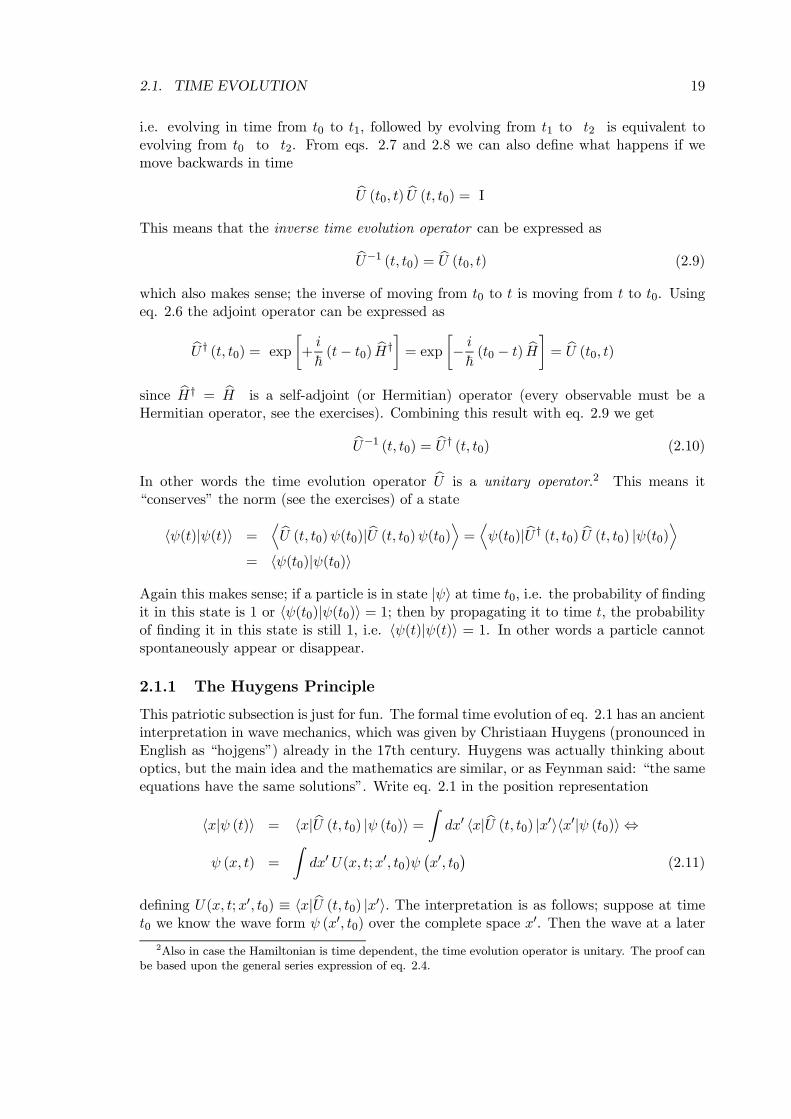
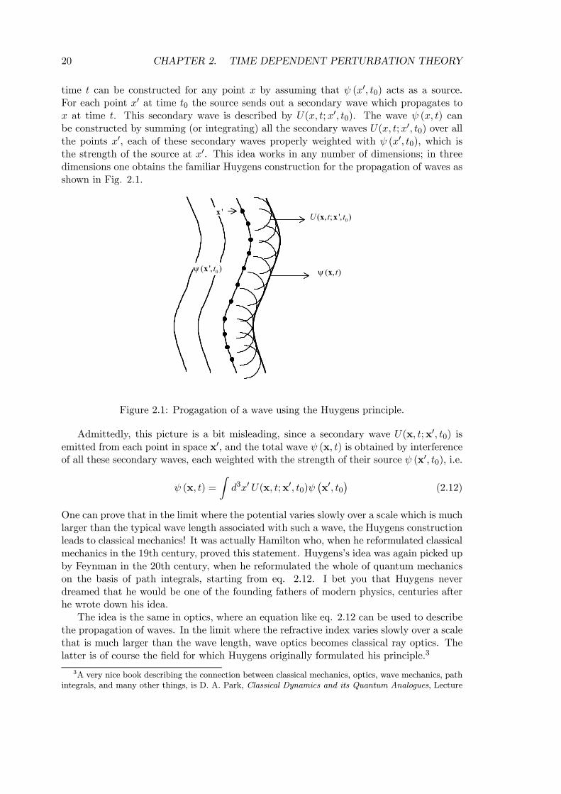
time t can be constructed for any point x by assuming that ψ (x0, t0) acts as a source.For each point x0 at time t0 the source sends out a secondary wave which propagates tox at time t. This secondary wave is described by U(x, t;x0, t0). The wave ψ (x, t) canbe constructed by summing (or integrating) all the secondary waves U(x, t;x0, t0) over allthe points x0, each of these secondary waves properly weighted with ψ (x0, t0), which isthe strength of the source at x0. This idea works in any number of dimensions; in threedimensions one obtains the familiar Huygens construction for the propagation of waves asshown in Fig. 2.1.
0( ', )tψ x
0( , ; ', )U t tx x
( , )tψ x
'x
0( ', )tψ x
0( , ; ', )U t tx x
( , )tψ x
'x
Figure 2.1: Progagation of a wave using the Huygens principle.
Admittedly, this picture is a bit misleading, since a secondary wave U(x, t;x0, t0) isemitted from each point in space x0, and the total wave ψ (x, t) is obtained by interferenceof all these secondary waves, each weighted with the strength of their source ψ (x0, t0), i.e.
ψ (x, t) =
Zd3x0 U(x, t;x0, t0)ψ
¡x0, t0
¢(2.12)
One can prove that in the limit where the potential varies slowly over a scale which is muchlarger than the typical wave length associated with such a wave, the Huygens constructionleads to classical mechanics! It was actually Hamilton who, when he reformulated classicalmechanics in the 19th century, proved this statement. Huygens’s idea was again picked upby Feynman in the 20th century, when he reformulated the whole of quantum mechanicson the basis of path integrals, starting from eq. 2.12. I bet you that Huygens neverdreamed that he would be one of the founding fathers of modern physics, centuries afterhe wrote down his idea.
The idea is the same in optics, where an equation like eq. 2.12 can be used to describethe propagation of waves. In the limit where the refractive index varies slowly over a scalethat is much larger than the wave length, wave optics becomes classical ray optics. Thelatter is of course the field for which Huygens originally formulated his principle.3
3A very nice book describing the connection between classical mechanics, optics, wave mechanics, pathintegrals, and many other things, is D. A. Park, Classical Dynamics and its Quantum Analogues, Lecture
2.2. TIME DEPENDENT PERTURBATIONS 21
2.2 Time Dependent Perturbations
Suppose we have a Hamiltonian
bH = bH0 + bV (t) (2.13)
where bH0 is the Hamiltonian of an unperturbed system (a molecule or a crystal, forinstance) and bV (t) is a small time-dependent perturbation (an external electromagneticfield, for instance). Furthermore suppose that we know all there is to know about theunperturbed system. In other words, we have solved the equation
i~∂
∂tbU0 (t, t0) = bH0 bU0 (t, t0) (2.14)
and we know the time evolution of the unperturbed system as given by bU0. We would ofcourse like to solve the full time evolution bU , including the perturbation,
i~∂
∂tbU (t, t0) = h bH0 + bV (t)i bU (t, t0) (2.15)
Since we know bU0 already, we split off this unperturbed part and define an operatorbUI (t, t0) by writingbU (t, t0) = bU0(t, t0)bUI (t, t0)⇔ bUI (t, t0) = bU †0 (t, t0) bU (t, t0) (2.16)
Use eq. 2.16 in eq. 2.15 (skipping the argument (t, t0) in the notation for the moment)
i~∂
∂t
hbU0 bUIi = bH0 bU0 bUI + bV (t) bU0 bUI applying the chain rule gives
⇐⇒·i~
∂
∂tbU0¸ bUI + bU0 ·i~ ∂
∂tbUI¸ = ·i~ ∂
∂tbU0¸ bUI + bV (t) bU0 bUI
where we have used eq. 2.14. Deleting the first terms at each side yields
bU0 ·i~ ∂∂tbUI¸ = bV (t) bU0 bUI
multiplying from the left with bU †0 and definingbVI(t) = bU †0(t, t0)bV (t)bU0(t, t0) (2.17)
finally gives
i~∂
∂tbUI(t, t0) = bVI(t)bUI(t, t0) (2.18)
We now have a Schrodinger like equation similar to eqs. 2.14, 2.15, but with a timeevolution which is determined by the perturbation bVI(t) only. We have achieved this bynotes in physics, Vol. 110 (Springer, Berlin, 1979).I would also suggest a wonderfull little booklet, written for the layman by one of physics’ heroes: R. P.
Feynman, QED, the strange theory of light and matter. A must-have for every physicist!!
22 CHAPTER 2. TIME DEPENDENT PERTURBATION THEORY
splitting off the time evolution bU0, which we already knew, and using eqs. 2.16 and 2.17.Quantities defined like in eq. 2.17, which we give the subscript I, constitute the so-calledinteraction picture. It resembles the Heisenberg picture discussed in Appendix I, cf. eq.2.63. The main idea of the interaction picture is to focus on the external perturbation(which is the “interaction”). We already know the formal solution of eq. 2.18 from theprevious section, namely eq. 2.3, or as a series, eq. 2.4.4 We can write
bUI (t, t0) = I + ∞Xn=1
bU (n)I (t, t0) (2.19)
where bU (n)I is a term of the series expansion
bU (n)I (t, t0) =
µ1
i~
¶n Z t
t0
dτn
Z τn
t0
dτn−1Z τn−1
t0
dτn−2......Z τ3
t0
dτ2
Z τ2
t0
dτ1
bVI (τn) bVI (τn−1) bVI (τn−2) ......bVI (τ2) bVI (τ1) (2.20)
The main idea should be clear by now. bUI is sort of a power series in bVI , with bU (n)I ∝ bV nI .One assumes that the perturbation bVI is small, hoping that the series converges quicklyand only the first few terms will be sufficient for a decent approximation. We can nowstep back from the “interaction picture” to our original “Schrodinger picture”. Using eqs.2.16, 2.17, 2.19 and 2.20 gives us our final result for the time evolution operator
bU (t, t0) = bU0 (t, t0) + ∞Xn=1
bU (n) (t, t0) (2.21)
where the first term on the right hand side describes the time evolution of the unperturbedsystem and the second term is a series of perturbation corrections. bU (n) is the term ofn’th order in the perturbation bV
bU (n) (t, t0) =
µ1
i~
¶n Z t
t0
dτn
Z τn
t0
dτn−1............Z τ3
t0
dτ2
Z τ2
t0
dτ1 (2.22)
bU0 (t, τn) bV (τn) bU0 (τn, τn−1) .......bU0 (τ3, τ2) bV (τ2) bU0 (τ2, τ1) bV (τ1) bU0 (τ1, t0)Perturbation theory is one of the most prominent tools in quantum mechanics, and expres-sions like eqs. 2.21, 2.22 are used all over the place. Richard Feynman invented a pictorialrepresentation for time integrals like eq. 2.22, based upon an intuitive “physical” inter-pretation. Starting from right to left in the integrand, the system moves “unperturbed”from the initial time t0 to a time τ1 described by bU0 (τ1, t0). At time τ1 an interactionwith the perturbing potential takes place, described by bV (τ1). Then the system againmoves unperturbed from time τ1 to τ2 before an interaction bV (τ2) takes place, etcetera.In a so-called Feynman diagram this is pictured as in Fig. 2.2.
The diagram is defined to be completely equivalent to eq. 2.22. The direction of thearrows gives the direction of time propagation. Each arrow describes an unperturbedpropagation between two times, and each dot (or vertex, as it is called mathematically)represents an interaction with the perturbation at a specific time. The dictionary thattranslates diagrams into mathematical equations is given in Fig. 2.3.
4Eqs. 2.5 and 2.6 are not valid here since bVI (t) is time dependent.

2.3. FERMI’S GOLDEN RULE 23
1τ0t t
2τ nτ
)( 1τV )( 2τV )( nV τ
a simple Feynman diagram
Figure 2.2: Feynman diagram.
1τ0t
1τ)(ˆ
11 τVi=
),(ˆ10 τtU=
Figure 2.3: Dictionary of Feynman diagrams.
Note that the constant 1i~ is absorbed in the interaction. Since the interactions can
take place at any time, integrations over the intermediate time labels τ1, τ2, ..., τn arealways assumed, also in the diagrams. The diagrams (and thus the integrals) are timeordered, i.e. t0 ≤ τ1 ≤ τ2.... ≤ τn ≤ t. The integrals are always written from right toleft, i.e. starting at the right with t0, and increasing the time when going to the left. Ithas to be like this since, by convention, operators work on states from right to left. Likemany other authors I write diagrams from left to right , since this is the natural order inwhich we are used to read. Some authors, like Mattuck, write diagrams from bottom totop. Several different conventions are used but confusion should not arise, since the arrowsalways indicate the direction of time flow and the points at which to start and stop.
As a diagram, Fig. 2.2 looks fairly trivial. Later on in many particle physics we will seemore much complicated diagrams. In addition we will see that manipulating diagrams issometimes easier than manipulating mathematical equations. Since we have a dictionarylike Fig. 2.3 to translate diagrams into equations and vice versa, we can always obtainone from the other.
2.3 Fermi’s Golden Rule
“The rule is jam tomorrow and jam yesterday - but never jam today”, Lewis Caroll, Through the
Looking-Glass.
The terms bU (n) (t, t0) in the perturbation series of eqs. 2.21 and 2.22 are, looselyspeaking, proportional to bV n. Now suppose the perturbation bV is very, very small. Itis then sufficient to consider the first order term only and neglect all higher order terms.
24 CHAPTER 2. TIME DEPENDENT PERTURBATION THEORY
This approximation is called the Born54 approximation.5
bU(t, t0) ≈ bU0(t, t0) + bU (1) (t, t0) = bU0 (t, t0) + 1
i~
Z t
t0
dτ bU0 (t, τ) bV (τ) bU0 (τ , t0) (2.23)
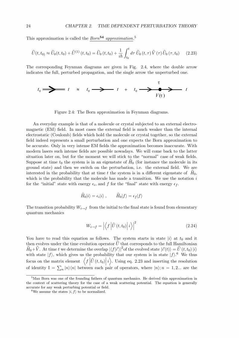
The corresponding Feynman diagrams are given in Fig. 2.4, where the double arrowindicates the full, perturbed propagation, and the single arrow the unperturbed one.
t0t ≈ t0t +τ
0t)(τV
t
Figure 2.4: The Born approximation in Feynman diagrams.
An everyday example is that of a molecule or crystal subjected to an external electro-magnetic (EM) field. In most cases the external field is much weaker than the internalelectrostatic (Coulomb) fields which hold the molecule or crystal together, so the externalfield indeed represents a small perturbation and one expects the Born approximation tobe accurate. Only in very intense EM fields the approximation becomes inaccurate. Withmodern lasers such intense fields are possible nowadays. We will come back to the lattersituation later on, but for the moment we will stick to the “normal” case of weak fields.Suppose at time t0 the system is in an eigenstate of bH0 (for instance the molecule in itsground state) and then we switch on the perturbation, i.e. the external field. We areinterested in the probability that at time t the system is in a different eigenstate of bH0,which is the probability that the molecule has made a transition. We use the notation ifor the “initial” state with energy ²i, and f for the “final” state with energy ²f .
bH0|ii = ²i|ii , bH0|fi = ²f |fiThe transition probabilityWi→f from the initial to the final state is found from elementaryquantum mechanics
Wi→f =¯Df¯ bU (t, t0)¯ iE¯2 (2.24)
You have to read this equation as follows. The system starts in state |ii at t0 and itthen evolves under the time evolution operator bU that corresponds to the full HamiltonianbH0+ bV . At time t we determine the overlap |hf |i0i|2of the evolved state |i0(t)i = bU (t, t0) |iiwith state |fi, which gives us the probability that our system is in state |fi.6 We thusfocus on the matrix element
Df¯ bU (t, t0)¯ iE. Using eq. 2.23 and inserting the resolution
of identity I =Pn |nihn| between each pair of operators, where |ni;n = 1, 2... are the
5Max Born was one of the founding fathers of quantum mechanics. He derived this approximation inthe context of scattering theory for the case of a weak scattering potential. The equation is generallyaccurate for any weak perturbing potential or field.
6We assume the states |i, fi to be normalized.
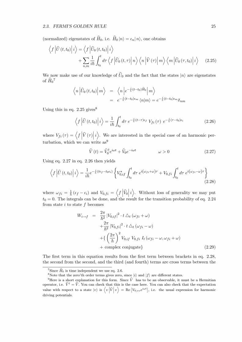
2.3. FERMI’S GOLDEN RULE 25
(normalized) eigenstates of bH0, i.e. bH0 |ni = ²n|ni, one obtainsDf¯ bU (t, t0)¯ iE = Df ¯ bU0 (t, t0)¯ iE
+Xn,m
1
i~
Z t
t0
dτDf¯ bU0 (t, τ)¯nEDn ¯ bV (τ)¯mEDm ¯ bU0 (τ , t0)¯ iE (2.25)
We now make use of our knowledge of bU0 and the fact that the states |ni are eigenstatesof bH07 D
n¯ bU0 (t, t0)¯mE =
Dn¯e−
i~ (t−t0) bH0 ¯mE
= e−i~ (t−t0)²m hn|mi = e− i
~ (t−t0)²mδnm
Using this in eq. 2.25 gives8Df¯ bU (t, t0)¯ iE = 1
i~
Z t
t0
dτ e−i~ (t−τ)²f Vfi (τ) e−
i~ (τ−t0)²i (2.26)
where Vfi (τ) =Df¯ bV (τ)¯ iE. We are interested in the special case of an harmonic per-
turbation, which we can write as9bV (t) = bV †0 eiωt + bV0e−iωt ω > 0 (2.27)
Using eq. 2.27 in eq. 2.26 then yieldsDf¯ bU (t, t0)¯ iE = 1
i~e−
i~ (t²f−t0²i)
½V ∗0,if
Z t
t0
dτ ei(ωfi+ω)τ + V0,fi
Z t
t0
dτ ei(ωfi−ω)τ¾(2.28)
where ωfi =1~ (²f − ²i) and V0,fi =
Df¯ bV0 ¯ iE. Without loss of generality we may put
t0 = 0. The integrals can be done, and the result for the transition probability of eq. 2.24from state i to state f becomes
Wi→f =2π
~2|V0,if |2 · t4t (ωfi + ω)
+2π
~2|V0,fi|2 · t4t (ωfi − ω)
+µ2π
~
¶2V0,if V0,fi It (ωfi − ω,ωfi + ω)
+ complex conjugate (2.29)
The first term in this equation results from the first term between brackets in eq. 2.28,the second from the second, and the third (and fourth) terms are cross terms between the
7Since bH0 is time independent we use eq. 2.6.8Note that the zero’th order terms gives zero, since |ii and |fi are different states.9Here is a short explanation for this form. Since bV has to be an observable, it must be a Hermitian
operator, i.e. bV † = bV . You can check that this is the case here. You can also check that the expectationvalue with respect to a state |υi is
Dυ¯ bV ¯ υE = Re
£V0,υυe
iωt¤, i.e. the usual expression for harmonic
driving potentials.
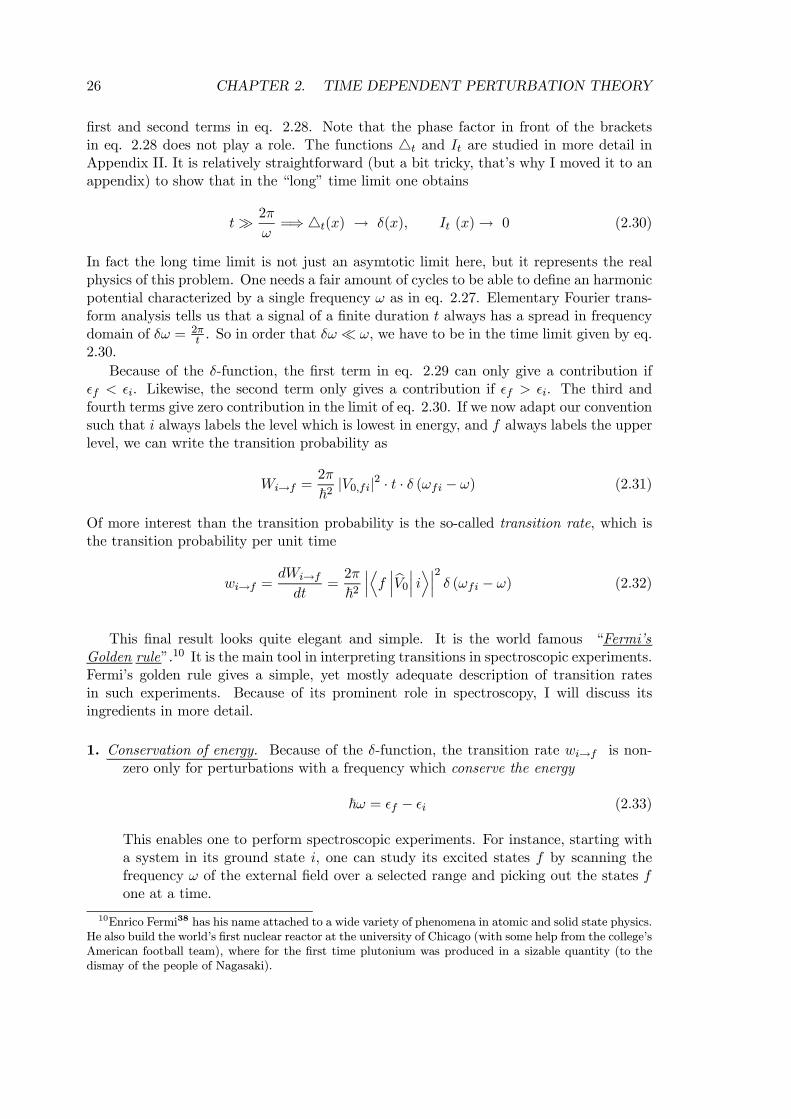
26 CHAPTER 2. TIME DEPENDENT PERTURBATION THEORY
first and second terms in eq. 2.28. Note that the phase factor in front of the bracketsin eq. 2.28 does not play a role. The functions 4t and It are studied in more detail inAppendix II. It is relatively straightforward (but a bit tricky, that’s why I moved it to anappendix) to show that in the “long” time limit one obtains
tÀ 2π
ω=⇒ 4t(x) → δ(x), It (x)→ 0 (2.30)
In fact the long time limit is not just an asymtotic limit here, but it represents the realphysics of this problem. One needs a fair amount of cycles to be able to define an harmonicpotential characterized by a single frequency ω as in eq. 2.27. Elementary Fourier trans-form analysis tells us that a signal of a finite duration t always has a spread in frequencydomain of δω = 2π
t . So in order that δω ¿ ω, we have to be in the time limit given by eq.2.30.
Because of the δ-function, the first term in eq. 2.29 can only give a contribution if²f < ²i. Likewise, the second term only gives a contribution if ²f > ²i. The third andfourth terms give zero contribution in the limit of eq. 2.30. If we now adapt our conventionsuch that i always labels the level which is lowest in energy, and f always labels the upperlevel, we can write the transition probability as
Wi→f =2π
~2|V0,fi|2 · t · δ (ωfi − ω) (2.31)
Of more interest than the transition probability is the so-called transition rate, which isthe transition probability per unit time
wi→f =dWi→fdt
=2π
~2¯Df¯ bV0 ¯ iE¯2 δ (ωfi − ω) (2.32)
This final result looks quite elegant and simple. It is the world famous “Fermi’sGolden rule”.10 It is the main tool in interpreting transitions in spectroscopic experiments.Fermi’s golden rule gives a simple, yet mostly adequate description of transition ratesin such experiments. Because of its prominent role in spectroscopy, I will discuss itsingredients in more detail.
1. Conservation of energy. Because of the δ-function, the transition rate wi→f is non-zero only for perturbations with a frequency which conserve the energy
~ω = ²f − ²i (2.33)
This enables one to perform spectroscopic experiments. For instance, starting witha system in its ground state i, one can study its excited states f by scanning thefrequency ω of the external field over a selected range and picking out the states fone at a time.
10Enrico Fermi38 has his name attached to a wide variety of phenomena in atomic and solid state physics.He also build the world’s first nuclear reactor at the university of Chicago (with some help from the college’sAmerican football team), where for the first time plutonium was produced in a sizable quantity (to thedismay of the people of Nagasaki).
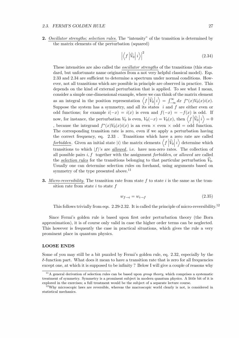
2.3. FERMI’S GOLDEN RULE 27
2. Oscillator strengths; selection rules. The “intensity” of the transition is determined bythe matrix elements of the perturbation (squared)¯D
f¯ bV0 ¯ iE¯2 (2.34)
These intensities are also called the oscillator strengths of the transitions (this stan-dard, but unfortunate name originates from a not very helpful classical model). Eqs.2.33 and 2.34 are sufficient to determine a spectrum under normal conditions. How-ever, not all transitions which are possible in principle are observed in practice. Thisdepends on the kind of external perturbation that is applied. To see what I mean,consider a simple one-dimensional example, where we can think of the matrix element
as an integral in the position representationDf¯ bV0 ¯ iE = R∞
−∞ dx f∗(x)V0(x)i(x).
Suppose the system has a symmetry, and all its states i and f are either even orodd functions; for example i(−x) = i(x) is even and f(−x) = −f(x) is odd. Ifnow, for instance, the perturbation V0 is even, V0(−x) = V0(x), then
Df¯ bV0 ¯ iE = 0
, because the integrand f∗(x)V0(x)i(x) is an even × even × odd = odd function.The corresponding transition rate is zero, even if we apply a perturbation havingthe correct frequency, eq. 2.33 . Transitions which have a zero rate are called
forbidden. Given an initial state |ii the matrix elementsDf¯ bV0 ¯ iE determine which
transitions to which |fi’s are allowed , i.e. have non-zero rates. The collection ofall possible pairs i, f together with the assignment forbidden, or allowed are calledthe selection rules for the transitions belonging to that particular perturbation bV0.Usually one can determine selection rules on forehand, using arguments based onsymmetry of the type presented above.11
3. Micro-reversibility. The transition rate from state f to state i is the same as the tran-sition rate from state i to state f
wf→i = wi→f (2.35)
This follows trivially from eqs. 2.29-2.32. It is called the principle of micro-reversibility.12
Since Fermi’s golden rule is based upon first order perturbation theory (the Bornapproximation), it is of course only valid in case the higher order terms can be neglected.This however is frequently the case in practical situations, which gives the rule a veryprominent place in quantum physics.
LOOSE ENDS
Some of you may still be a bit puzzled by Fermi’s golden rule, eq. 2.32, especially by theδ-function part. What does it mean to have a transition rate that is zero for all frequenciesexcept one, at which it is supposed to be infinity ? Below I will give a couple of reasons why
11A general derivation of selection rules can be based upon group theory, which comprises a systematictreatment of symmetry. Symmetry is a prominent subject in modern quantum physics. A little bit of it isexplored in the exercises; a full treatment would be the subject of a separate lecture course.12Why microscopic laws are reversible, whereas the macroscopic world clearly is not, is considered in
statistical mechanics.
28 CHAPTER 2. TIME DEPENDENT PERTURBATION THEORY
in real physical measurements one never really obtains δ-functions, but (at best) sharplypeaked function with a finite height and a finite width.
1. For finite times t, the function 4t(ωfi−ω) in eq. 2.29 will of course not be exactly a δ-function. A picture of this function is shown in Fig. 2.8 (see Appendix II). StandardFourier analysis shows that this function has a finite width δω ' 2π
t ¿ ω aroundits center at ωfi − ω = 0. In optical absorption spectroscopy typically t À 10−6 s,so δω ¿ 106 Hz. (mind you, these are order-of-magnitude numbers to give you justan impression). A typical optical frequency is ω v 1015 Hz, which is also a measurefor the frequency scan in a spectroscopic experiment. This means that δω
ω is indeedvery small. In fact, it is usually too small to be of any practical interest and thus wecan mathematically approximate 4t by a δ-function and It by zero as in eq. 2.30.
2. The second reason is more or less the same as the first, but it focuses more on the sourceof the perturbing potential. We started with a pure harmonic driving potential in eq.2.27. Such a perfect monochromatic potential is ideal to work with mathematically,but physically it is a bit artificial, since in practice it can never be achieved. As anexample, electromagnetic (EM) radiation is one of the most commonly used sourcesfor harmonic driving potentials. EM waves can be made monochromatic to a gooddegree (by using lasers, for instance), but never perfectly; there will always be a small,but finite, frequency spread. So instead of eq. 2.27 we should have used a potential of
the formR hbV †0 (ω0)eiω0t + bV0(ω0)e−iω0ti dω0. For a nearly monochromatic potentialbV0(ω0) is sharply peaked around a central frequency ω0 and it goes rapidly to zero
for an ω0 away from ω0. The whole calculation of eqs. 2.28-2.32 can also be done forthis “nearly monochromatic potential”, but the expressions become clumsy, so I willonly give you the flavor. Eqs. 2.29-2.32 will contain a large number of cross terms
between different frequencies of a typeDf¯ bV0(ω0)¯ iEDf ¯ bV0(ω00)¯ iE. If we assume
that the phases of all these factors for different frequencies are unrelated (and thisis indeed the case for the usual sources), then one can show that the sum of all suchcross terms is zero. The resulting expression then becomes a rather simple extensionof eq. 2.32
wi→f =2π
~2
Z ¯Df¯ bV0(ω0)¯ iE¯2 δ ¡ωfi − ω0
¢dω0 (2.36)
We define an oscillator strength gfi by a simple extension of eq. 2.34 as
gfi =
Z ¯Df¯ bV0(ω0)¯ iE¯2 dω0 (2.37)
Now we formally define a line-shape function F (ω0 − ω0) by
F (ω0 − ω0) =1
gfi
¯Df¯ bV0(ω0)¯ iE¯2 (2.38)
Since we assumed that bV0(ω0) is sharply peaked around ω0 = ω0, F (ω0 − ω0) is
sharply peaked around 0; let us call the typical width of this peak 4ω. Note that
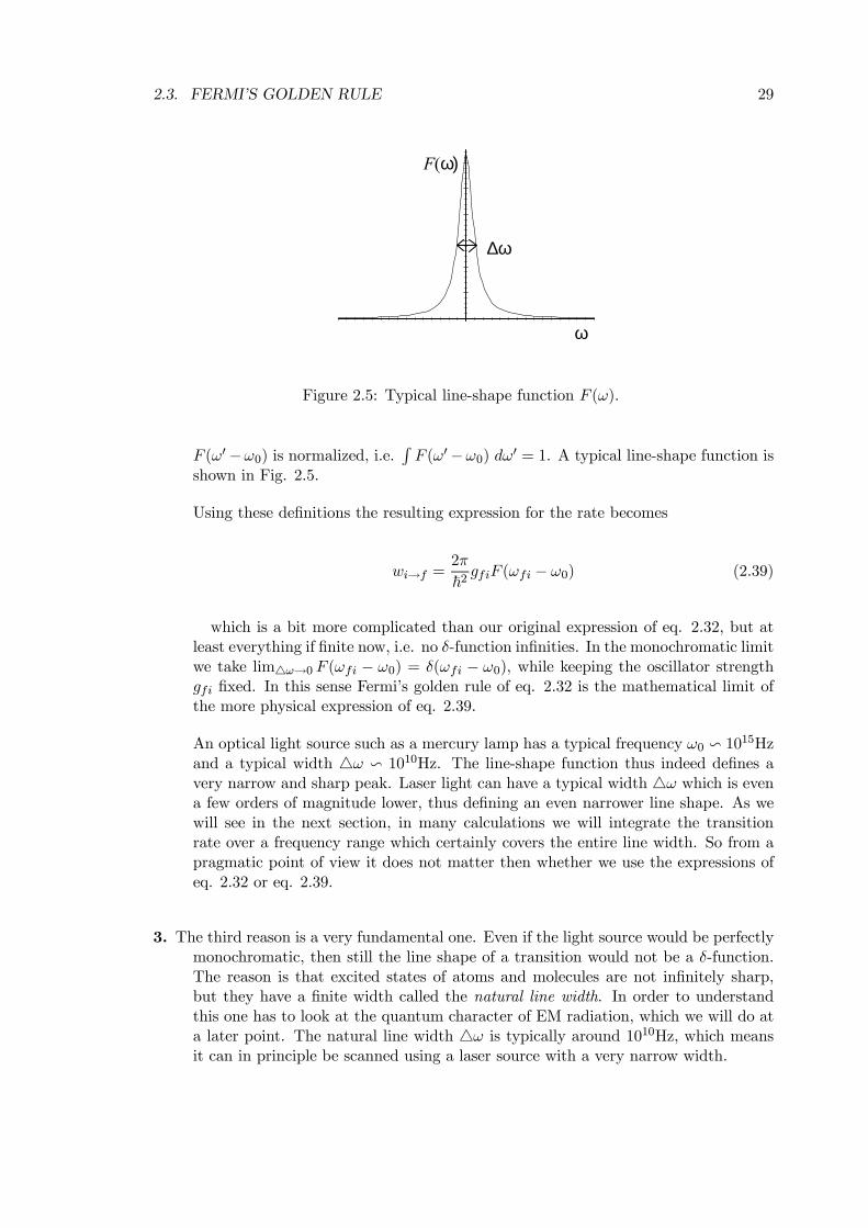
2.3. FERMI’S GOLDEN RULE 29
ω
F(ω)
∆ω
Figure 2.5: Typical line-shape function F (ω).
F (ω0−ω0) is normalized, i.e.RF (ω0−ω0) dω
0 = 1. A typical line-shape function isshown in Fig. 2.5.
Using these definitions the resulting expression for the rate becomes
wi→f =2π
~2gfiF (ωfi − ω0) (2.39)
which is a bit more complicated than our original expression of eq. 2.32, but atleast everything if finite now, i.e. no δ-function infinities. In the monochromatic limitwe take lim4ω→0 F (ωfi − ω0) = δ(ωfi − ω0), while keeping the oscillator strengthgfi fixed. In this sense Fermi’s golden rule of eq. 2.32 is the mathematical limit ofthe more physical expression of eq. 2.39.
An optical light source such as a mercury lamp has a typical frequency ω0 v 1015Hzand a typical width 4ω v 1010Hz. The line-shape function thus indeed defines avery narrow and sharp peak. Laser light can have a typical width 4ω which is evena few orders of magnitude lower, thus defining an even narrower line shape. As wewill see in the next section, in many calculations we will integrate the transitionrate over a frequency range which certainly covers the entire line width. So from apragmatic point of view it does not matter then whether we use the expressions ofeq. 2.32 or eq. 2.39.
3. The third reason is a very fundamental one. Even if the light source would be perfectlymonochromatic, then still the line shape of a transition would not be a δ-function.The reason is that excited states of atoms and molecules are not infinitely sharp,but they have a finite width called the natural line width. In order to understandthis one has to look at the quantum character of EM radiation, which we will do ata later point. The natural line width 4ω is typically around 1010Hz, which meansit can in principle be scanned using a laser source with a very narrow width.
30 CHAPTER 2. TIME DEPENDENT PERTURBATION THEORY
2.4 Radiative Transitions
2.4.1 Atom in a Radiation Field
Detailed applications of quantum mechanics are not part of this course; they are supposedto be part of (advanced) courses on molecular or condensed matter physics, for example.Yet Fermi’s golden rule plays such an important role in the interpretation of all kindsof spectroscopy that I will consider its application in somewhat more detail by a simple,yet physical, example of an atom or molecule in an external electromagnetic field. Thecomplete Hamiltonian which describes the interaction between an electromagnetic fieldand matter has a somewhat complicated form. A full discussion of it is not possiblewithin the constraints of this course, so I will present a simplified description, which isnot wrong, but limited.
Consider an electromagnetic (EM) wave, the electric part of which is given by
E (r, t) =
E000
cos (kz − ωt) (2.40)
The electric field E oscillates along the x-direction, and z is the direction of wave propa-gation. The magnetic part of the wave is then of course given by
B(r, t) =
0B00
cos (kz − ωt)
The size of an atom or molecule is typically in the range 1-10A, whereas the wave lengthλ = 2π
k of visible light is typically in the range 4-8× 10³A. To a very good approximationwe may therefore neglect the spatial dependence of the EM wave over the molecule andtreat the fields as homogeneous, i.e. spatially independent. For a molecule in the originwe can use z = 0 in eq. 2.40. All electric charges in the molecule interact with the electricfield. Assuming that the molecule as a whole is neutral, its energy V in a uniform electricfield E is given by simple electrostatics as
V = −µ ·E where µ =NXI=1
ZIRI − enXi=1
ri (2.41)
is the total dipole moment of the molecule; ZI , RI are the charges and positions of thenuclei, −e and ri are the charges and positions of the electrons and N,n are the number ofnuclei and electrons, respectively. We now assume that the correct quantum mechanicaloperator is given by bV = −bµ ·E (2.42)
where bµ is the dipole moment operator, which is the same expression as eq. 2.41, butwith positions replaced by position operators. Using eqs. 2.40 and 2.41 and the spatialhomogeneity of the field we get bV (t) = −bµxE0 cosωt (2.43)
A couple of questions might puzzle the critical observer
2.4. RADIATIVE TRANSITIONS 31
• Is there no interaction with the magnetic field? Yes there is, but a more elaboratetreatment shows that this interaction is much weaker, so we neglect it here. It givesrise to much weaker magnetic dipole transitions.
• What happens if the molecule is larger and/or the wave length is shorter such thatwe may no longer assume that the electric field is homogeneous? We have to do amultipole expansion and consider quadrupoles and higher multipoles.
• What if we have a very large system for which we expect even a multipole expansionto be invalid, such as, for instance, a crystal. Or what happens if we use very shortwave length radiation, such as X rays. In those cases we have to take a differentapproach right from the start, which (hopefully) you will find in your advancedtopical courses.
Let’s now consider the “simplest” system: a hydrogen atom.13 The dipole moment ofa hydrogen atom is simply µ = −er, where r points from the proton to the electron, soeq. 2.43 becomes
bV (t) = ebxE0 cosωt = ebxE02(eiωt + e−iωt) (2.44)
Fermi’s Golden rule, eq. 2.32, gives for the transition rate between two states of thehydrogen atom
wi→f =πe2
2~2E20 |hf |bx| ii|2 δ (ωfi − ω) (2.45)
The cycle averaged intensity I of the EM wave is proportional to I v E20 . In other wordsthe transition rate is proportional to the intensity of the EM wave. This is called the linearterm. If, instead of using only first order perturbation theory, we use additional higherorder n = 2, 3... perturbation terms in eq. 2.23, the latter lead to terms in the transitionrate that are proportional to In;n = 2, 3... These higher order terms are collectively calledthe non-linear terms. Usually, in ordinary spectroscopy the intensity is sufficiently smallsuch that the linear term is by far dominant. In very intense laser beams the non-linearterms can become non-negligible. We are then in the realm of non-linear spectroscopy,where Fermi’s gold no longer rules alone, but in principle you know how to produce newrules; simply add higher order perturbation terms. It is not too difficult to prove that inan “ordinary” laser beam, where E0 ∼ 103 V/m, even the Fermi Golden rule rate wi→f ,eq. 2.45, is small and higher order terms are certainly negligible (see the exercises).
Some final remarks concerning eq. 2.45
• |hf |bx| ii|2 is of dimension “surface” ¡m2¢ and in fact of order a20 (where a0 =0.529177249× 10⁻¹⁰m is the Bohr radius of the hydrogen atom). It roughly corre-sponds to the “size” of a cross-section through the hydrogen atom and is thereforecalled the absorption cross-section . This holds for a molecule in general, the absorp-tion cross section is proportional to the size of the molecule.
13Conceptually, a general molecule is not more complicated in principle, but the notation gets a bitmessy. In practical calculations, a general molecule is just more work (actually a lot more).
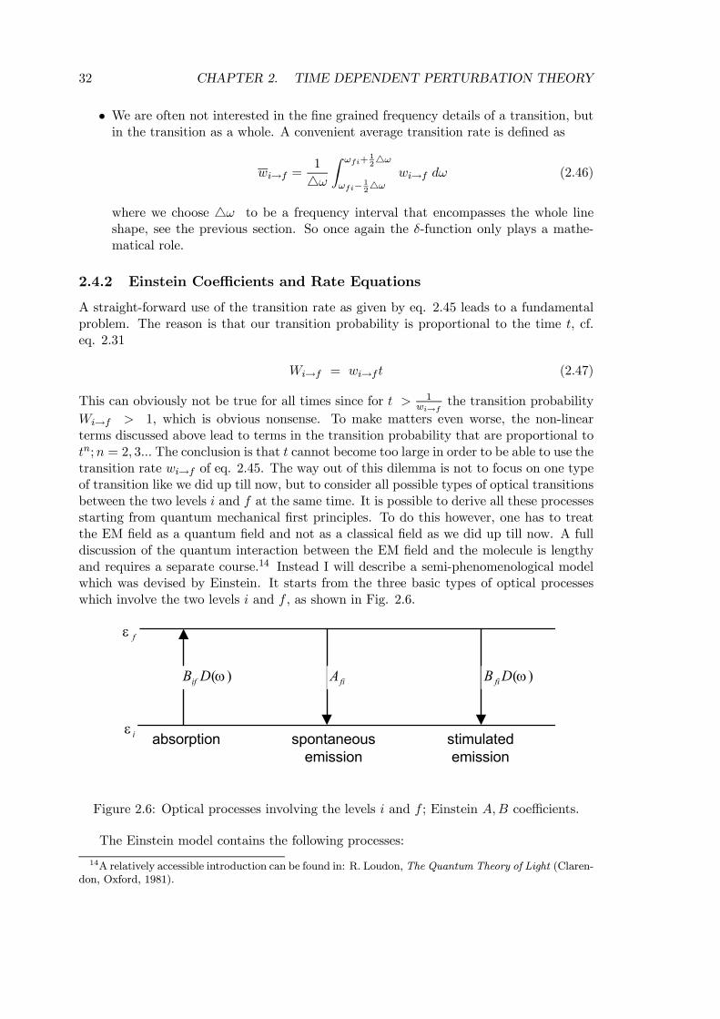
32 CHAPTER 2. TIME DEPENDENT PERTURBATION THEORY
• We are often not interested in the fine grained frequency details of a transition, butin the transition as a whole. A convenient average transition rate is defined as
wi→f =1
4ω
Z ωfi+124ω
ωfi− 124ω
wi→f dω (2.46)
where we choose 4ω to be a frequency interval that encompasses the whole lineshape, see the previous section. So once again the δ-function only plays a mathe-matical role.
2.4.2 Einstein Coefficients and Rate Equations
A straight-forward use of the transition rate as given by eq. 2.45 leads to a fundamentalproblem. The reason is that our transition probability is proportional to the time t, cf.eq. 2.31
Wi→f = wi→f t (2.47)
This can obviously not be true for all times since for t > 1wi→f
the transition probability
Wi→f > 1, which is obvious nonsense. To make matters even worse, the non-linearterms discussed above lead to terms in the transition probability that are proportional totn;n = 2, 3... The conclusion is that t cannot become too large in order to be able to use thetransition rate wi→f of eq. 2.45. The way out of this dilemma is not to focus on one typeof transition like we did up till now, but to consider all possible types of optical transitionsbetween the two levels i and f at the same time. It is possible to derive all these processesstarting from quantum mechanical first principles. To do this however, one has to treatthe EM field as a quantum field and not as a classical field as we did up till now. A fulldiscussion of the quantum interaction between the EM field and the molecule is lengthyand requires a separate course.14 Instead I will describe a semi-phenomenological modelwhich was devised by Einstein. It starts from the three basic types of optical processeswhich involve the two levels i and f , as shown in Fig. 2.6.
)(ωDBif )(ωDBfifiA
absorption spontaneousemission
stimulatedemission
fε
iε
Figure 2.6: Optical processes involving the levels i and f ; Einstein A,B coefficients.
The Einstein model contains the following processes:
14A relatively accessible introduction can be found in: R. Loudon, The Quantum Theory of Light (Claren-don, Oxford, 1981).
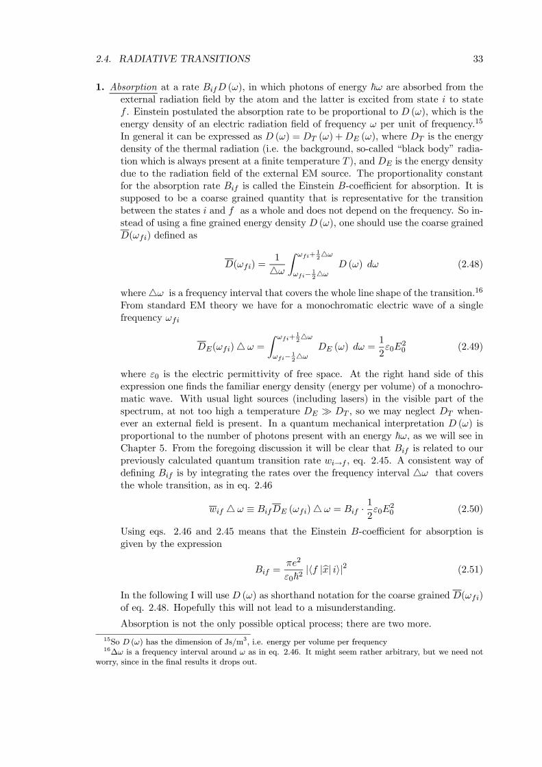
2.4. RADIATIVE TRANSITIONS 33
1. Absorption at a rate BifD (ω), in which photons of energy ~ω are absorbed from theexternal radiation field by the atom and the latter is excited from state i to statef . Einstein postulated the absorption rate to be proportional to D (ω), which is theenergy density of an electric radiation field of frequency ω per unit of frequency.15
In general it can be expressed as D (ω) = DT (ω) +DE (ω), where DT is the energydensity of the thermal radiation (i.e. the background, so-called “black body” radia-tion which is always present at a finite temperature T ), and DE is the energy densitydue to the radiation field of the external EM source. The proportionality constantfor the absorption rate Bif is called the Einstein B-coefficient for absorption. It issupposed to be a coarse grained quantity that is representative for the transitionbetween the states i and f as a whole and does not depend on the frequency. So in-stead of using a fine grained energy density D (ω), one should use the coarse grainedD(ωfi) defined as
D(ωfi) =1
4ω
Z ωfi+124ω
ωfi− 124ω
D (ω) dω (2.48)
where4ω is a frequency interval that covers the whole line shape of the transition.16
From standard EM theory we have for a monochromatic electric wave of a singlefrequency ωfi
DE(ωfi)4 ω =
Z ωfi+124ω
ωfi−124ω
DE (ω) dω =1
2ε0E
20 (2.49)
where ε0 is the electric permittivity of free space. At the right hand side of thisexpression one finds the familiar energy density (energy per volume) of a monochro-matic wave. With usual light sources (including lasers) in the visible part of thespectrum, at not too high a temperature DE À DT , so we may neglect DT when-ever an external field is present. In a quantum mechanical interpretation D (ω) isproportional to the number of photons present with an energy ~ω, as we will see inChapter 5. From the foregoing discussion it will be clear that Bif is related to ourpreviously calculated quantum transition rate wi→f , eq. 2.45. A consistent way ofdefining Bif is by integrating the rates over the frequency interval 4ω that coversthe whole transition, as in eq. 2.46
wif 4 ω ≡ BifDE (ωfi)4 ω = Bif · 12ε0E
20 (2.50)
Using eqs. 2.46 and 2.45 means that the Einstein B-coefficient for absorption isgiven by the expression
Bif =πe2
ε0~2|hf |bx| ii|2 (2.51)
In the following I will use D (ω) as shorthand notation for the coarse grained D(ωfi)of eq. 2.48. Hopefully this will not lead to a misunderstanding.
Absorption is not the only possible optical process; there are two more.
15So D (ω) has the dimension of Js/m3, i.e. energy per volume per frequency16∆ω is a frequency interval around ω as in eq. 2.46. It might seem rather arbitrary, but we need not
worry, since in the final results it drops out.
34 CHAPTER 2. TIME DEPENDENT PERTURBATION THEORY
2. Stimulated emission at a rate BfiD (ω), in which photons of energy ~ω are put backinto exactly the same mode as that of the external radiation field, i.e. at the samefrequency and direction as the external field. The atom is de-excited from state fto state i.
3. Spontaneous emission at a rate Afi, in which also photons of energy ~ω are send out,but in any mode. Spontaneously emitted photons can have any direction. In fact,the probability that a spontaneously emitted photon has the same direction as theincoming field is negligibly small.
The difference between stimulated and spontaneous emission is shown schematicallyin Fig. 2.7.
incomingwave
spontaneousemission
non-absorbed radiation +stimulated emission
Figure 2.7: Radiative processes.
In summary, Bif , Afi and Bfi are called the Einstein coefficients for the absorption,spontaneous and stimulated emission and Figs. 2.6 and 2.7 summarize the Einstein modelfor radiative processes.17 Remarkably, the A,B coefficients are not independent but theyare related by
Bif = Bfi ;
µ~ω3
π2c3
¶Bfi = Afi (2.52)
Proof: As remarked before, these relations can in principle be proven from basicquantum mechanics, but the proof is lengthy. Einstein gave a very elegant alternativeproof, which is essentially based upon statistical physics. Call the occupation probability(or population) of the lower level Ni, and that of the upper level Nf . The system issupposed to be in one of these two states, so Ni +Nf = 1. If the processes given in Fig.2.6 are the only ones possible, we can write down a phenomenological rate equation forthese populations
dNidt
= −dNfdt
= −NiBifD (ω) +NfBfiD (ω) +NfAfi (2.53)
The rate NfAfi at which the upper level f is depopulated by spontaneous emission isgiven by the transition rate Afi times its population Nf , etcetera. It is identical to the
17In various branches of physics there are Einstein models around, since Einstein was a very active manwho worked on very diverse problems in his younger years. Einstein’s A and B coefficients are still usedtoday.
2.4. RADIATIVE TRANSITIONS 35
rate at which the lower level i is populated, since the system has to be in one of these twostates. In thermal equilibrium, in absence of any external radiation, the level populationsmust be constant (which is what equilibrium means) so
dNidt
= −dNfdt
= 0 (2.54)
From eq. 2.53 we then obtain the energy density of the thermal radiation, which is presentin thermal equilibrium
DT (ω) =Afi
(Ni/Nf )Bif −BfiIn addition we know from statistical physics that in thermal equilibrium the level popula-tions are related by a Boltzmann factor, i.e.
NfNi
= e−~ωkT
using eq. 2.33. This yields
DT (ω) =Afi
e~ωkT Bif −Bfi
(2.55)
On the other hand, the energy density of thermal (black body) radiation is also given byPlanck’s law18
DT (ω) =~ω3
π2c31
e~ωkT − 1
(2.56)
For the two expressions of eqs. 2.55 and 2.56 to be identical, the A,B coefficients mustbe related as in eq. 2.52.
2.4.3 Population and Lifetime
Back to our main route; we now apply the external radiation field and neglect the thermalradiation field. The rate equations of eq. 2.53 can be solved in a straightforward wayNi+Nf = 1. Starting from the initial conditions Ni(0) = 1 and Nf (0) = 0 the solution is
Nf (t) =
µAfiBifDE
+ 2
¶−11− exp [− (Afi + 2BifDE) t] (2.57)
Ni(t) = 1−Nf (t)
using Ni +Nf = 1. Since rates are always positive, the population Nf (t) increases mono-tonically in time, but only to a maximum
Nf (∞) =µ
AfiBifDE
+ 2
¶−1(2.58)
18See e.g. S Gasiorowicz, Quantum Physics, (Wiley, New York, 1974), Ch.1, or B. H. Brandsen & C. J.Joachain, Quantum Mechanics, (Prentice Hall, New Jersey, 2000), Ch. 1.
36 CHAPTER 2. TIME DEPENDENT PERTURBATION THEORY
One observes that always Nf (t) <12 , which means that Ni(t) >
12 and thus Nf (t) <
Ni(t). For light sources of ordinary intensity (including most lasers) the spontaneousemission dominates, i.e. Afi À BifDE. This yields Nf ¿ 1
2 and Nf ¿ Ni, i.e. theupper level is much less populated than the lower level. The net rate of loss of energyfrom the incoming beam of radiation in the propagation direction is equal to the rateNiBifDE at which photons are taken out of the beam by absorption minus the rateNfBifDE at which photons are put back into the beam by stimulated emission, since theprobability that spontaneous emission puts a photon back in the propagation direction isnegligible. In other words the net rate of loss of energy from the incoming beam is givenby (Ni−Nf )BifDE~ω. One loosely speaks of “absorption” of light to describe this result,although strictly speaking this is not correct, since all three optical processes are involved.The fact that always Nf < Ni indeed shows that the beam is attenuated. If we could finda way such that Nf > Ni, which is called population inversion, then the beam intensitywould be amplified. We would have energy gain instead of energy loss, or in other wordswe would have produced a laser. The foregoing analysis shows that population inversionis impossible in a simple two-level system. Other tricks have to be used to get a laser; forinstance, a three-level system.
Note that by considering rate equations involving all three optical processes we obtaina finite (and usually small) population of the upper level, which solves the problem we hadwith eq. 2.47. “To shed more light on it”, suppose at a time t1 we turn off the external EMfield when the occupation of the upper level is Nf,1 ≡ Nf (t1). In absence of an externalfield and, as usual, neglecting the thermal radiation field, spontaneous emission is the onlyoptical process left. The upper level depopulates by spontaneous emission
dNfdt
= −NfAfi ⇒ Nf (t) = Nf,1e−Afit (2.59)
The characteristic time τR =1Afi
is called the radiative lifetime (also called the fluorescent
lifetime) of the level f . The quantum mechanical expression for the hydrogen atom is givenby
τ−1R = Afi =e2ω3
ε0π~c3|hf |bx| ii|2 (2.60)
using eqs. 2.51 and 2.52. A typical value is τR ∼ 10−9s. The typical time t to be insertedthen in eq. 2.47 to calculate the transition probability is of order τR, since after that timethe state f , populated by absorption, is depopulated again by emission. It is as if we aretrying to fill a bucket f which has a large hole in it. The time τR is long enough comparedto the “optical” time τ v ω−1 v 10−15s to make the “near δ-function” approximationdiscussed below eq. 2.35 valid. However, it is short enough for the transition probabilityof eq. 2.47 Wi→f ¿ 1, as one can easily prove by a direct calculation. This shows thatour analysis of the problem is internally consistent.
2.5 Epilogue
The discussion regarding radiative processes was not completely satisfactory from a fun-damental point of view (at least in my opinion).
2.6. APPENDIX I. THE HEISENBERG PICTURE 37
1. We had to involve some delicate assumptions in Section 2.4 regarding the observationtime scale t. It should be large enough to get a sharply peaked δ-like transitionline shape, but small enough such that the transition probability Wi→f would notgrow to an unphysically large value. By using the phenomenological Einstein modelfor absorption and emission of radiation we could argue that the lifetime of theexcited state τR sets the physical time scale t. The numerical values of the Einsteincoefficients in “normal” (i.e. not too strong) radiation fields are consistent with ourassumptions regarding this time scale, which is somewhat reassuring.
2. Our quantum mechanical treatment of the external field as a perturbation can de-scribe the absorption Wi→f and the stimulated emission Wf→i rates using Fermi’sgolden rule. However it cannot describe spontaneous emission (we needed the phe-nomenological Einstein model to do that). Once the external field is switched off,the perturbation is gone and the system can stay in an excited state forever, sinceit is an eigenstate of the unperturbed Hamiltonian bH0. This is clear nonsense, sincewe know experimentally that excited states have a finite lifetime τR.
3. Another unsatisfactory point is that, whereas we treated our hydrogen atom quan-tum mechanically, we assumed the external radiation field to be given by the classicalexpression of eq. 2.40. We mentioned photons, but where are they in the theory ?
All these problems have the same origin ! If we want to understand the full behaviorof a quantum system, we have to treat everything quantum mechanically, including theexternal fields. The full quantum mechanical Hamiltonian contains an atom, moleculeor crystal part as before, but also a term describing the (quantum) radiation field, aswell as a term that describes the coupling between the atom/molecule and the radiationfield. It is this last term that can be considered as a perturbation term. As we will see inChapter 5, the states of the radiation field can be interpreted in terms of quantum particlescalled photons. The “ground state” of the radiation field then is a state describing thesituation in which there are no photons present (this is the lowest energy state). The firstexcited state contains one photon, etcetera. The coupling term in the total Hamiltoniancan describe a transition between (1) a molecule in an excited state (f) + the radiationfield in its ground state (no photons) and (2) the molecule in its ground state (i) + theradiation field in its first excited state (one photon). This is what we call spontaneousemission! The details of this problem require a lengthy discussion, so we will not pursueit here.
2.6 Appendix I. The Heisenberg Picture
Just before Schrodinger formulated his wave mechanics, another form of quantum me-chanics was formulated by Heisenberg. The latter is nowadays called the Heisenberg pic-ture, whereas the form of quantum mechanics introduced in the first chapter is called theSchrodinger picture. Both these pictures appeared to be able to solve the same problems,such as the spectrum of the hydrogen atom, so for a while in the 1920’s people were puzzledby the fact that two apparently quite different quantum theories existed that both gavethe same results for measurable quantities. The main difference between the two picturesis the way in which time evolution is treated. Later on it was realized how these two pic-tures are connected and in the modern formulation of quantum mechanics, using the time
38 CHAPTER 2. TIME DEPENDENT PERTURBATION THEORY
evolution operator, we will see that the relation between the two pictures is almost trivial.I will briefly discuss the Heisenberg picture here. Since it focuses on operators, ratherthan on states, it still has a lot of relevance to modern quantum mechanics, especially toquantum field theory.
I will restrict the discussion to operators that do not explicitly depend on time. In theSchrodinger picture such operators bAS are fixed, i.e. time independent. I use the subscript“S” to indicate the Schrodinger picture. The states |ψS(t)i are of course time dependent.Their time evolution is given by the Schrodinger equation, and from Section 2.1 we knowthat formally the solution can be given as
|ψS(t)i = bU(t, t0)|ψS(t0)i (2.61)
where t0 is some fixed starting point in time. The states in the Heisenberg picture aresimply defined as
|ψHi ≡ |ψS(t0)i = bU †(t, t0)|ψS(t)i (2.62)
using eq. 2.10 and using the subscript “H” to indicate the Heisenberg picture. Note thatthe states in the Heisenberg picture are fixed, i.e. time independent. The Heisenbergoperators bAH(t) are considered to be time dependent. Their time dependence can bededuced from the fact that expectation values, which are the measurable quantities, mustbe identical in both the Schrodinger and Heisenberg pictures.
hψS(t)| bAS|ψS(t)i = hψS(t0)|bU †(t, t0) bAS bU(t, t0)|ψS(t0)i= hψH | bAH(t)|ψHi
using eq. 2.61. From the definition eq. 2.62 it is then self-evident that one must definebAH(t) = bU †(t, t0) bAS bU(t, t0) (2.63)
Note that at the starting point Heisenberg and Schrodinger operators are identical, i.e.bAH(t0) = bAS (2.64)
The algebra of Heisenberg operators is the same as that of Schrodinger operators, providedwe look at “equal times”. One can easily prove from eq. 2.63 thath bAS, bBSi = bCS ⇔ h bAH(t), bBH(t)i = bCH(t) (2.65)
Note that the commutatorh bAH(t), bBH(t0)i ; t 6= t0 is not so easy to derive, but luckily we
won’t be needing it.
All that is needed now is to derive an equation that describes the time evolution ofthese Heisenberg operators.
i~d bAH(t)dt
= i~d
dt
³bU †(t, t0) bAS bU(t, t0)´= bU †(t, t0) bAS Ãi~dbU(t, t0)
dt
!+
Ãi~dbU †(t, t0)
dt
! bAS bU(t, t0)= bU †(t, t0) bAS bHS bU(t, t0)− bU †(t, t0) bHS bAS bU(t, t0)
2.6. APPENDIX I. THE HEISENBERG PICTURE 39
where the Schrodinger equation, eq. 2.2, and its complex conjugate is used to derive thelast line. One can use eqs. 2.10 and 2.63 to transform the last line into
i~d bAH(t)dt
= bU †(t, t0) bAS bU(t, t0)bU †(t, t0) bHS bU(t, t0)− bU †(t, t0) bHS bU(t, t0)bU †(t, t0) bAS bU(t, t0)= bAH(t) bHH(t)− bHH(t) bAH(t)
The last line can be condensed to give the final result.
i~d bAH(t)dt
=h bAH(t), bHH(t)i (2.66)
This is called the Heisenberg equation. It describes time evolution in the Heisenberg pic-ture, and it obviously plays the same role as the Schrodinger equation in the Schrodingerpicture.
In summary, the Heisenberg picture is characterized by fixed states and time dependentoperators, whereas in the Schrodinger picture it is the other way around, i.e. fixed operatorsand time dependent states. Time evolution in the Heisenberg picture is given by theHeisenberg equation, eq. 2.66. Obviously both pictures give the same expectation valuesand thus the same measurable quantities. In fact the relation between the two pictures isgiven by a unitary transformation defined by the time evolution operator, cf. eqs. 2.62and 2.63.
In view of the simple relation between the two pictures, one might wonder what thefuss in the 1920’s was about. Well, Heisenberg used a completely different route to arriveat his equation, eq. 2.66, which at first sight indeed looks very different from the waveequation derived by Schrodinger. Heisenberg started from the classical Hamilton equa-tions of motion. We shall work our way backwards. Consider a simple one-dimensional
Hamiltonian bH = bp22m + V (bx). We drop the subscript “H” and assume that we are in the
Heisenberg picture. Using eq. 2.66 and the commutation relation [bx(t), bp(t)] = i~, it isthen straightforward to show that the time propagation of the position and momentumoperators is given by
dbx(t)dt
=bpm
anddbp(t)dt
= −dV (bx)dbx (2.67)
These equations look the same as the Hamilton equations of motion, except that herethe quantities are operators bx, bp instead of simple numbers x, p as they are in classicalmechanics. As usual the step from quantum to classical mechanics is easy —one dropsthe operator aspects— but the other way around is not easy, if you have to invent theconcept of operators first. Heisenberg did just that; at some point he realized that inquantum mechanics bx, bp are non-commutating quantities, unlike in classical mechanics.By a clever reasoning he succeeded in deriving the commutation relation [bx(t), bp(t)] = i~and from there he derived his time evolution equation 2.66, which, by the way, also leadhim to his famous uncertainty principle. The Heisenberg route is still in practice today,especially in quantum field theory. Consider for instance the electro-magnetic (EM) field.From Maxwell’s equations it is possible to derive a classical Hamiltonian. It proves tobe difficult to write down quantum states (for a good reason, there aren’t any quantum
40 CHAPTER 2. TIME DEPENDENT PERTURBATION THEORY
mechanical wave functions associated with the EM field). This hinders the Schrodingerroute to quantization, since it is difficult to guess a correct Schrodinger equation for the EMfield without having the states. But it is possible to identify “position” and “momentum”operators for the EM field and by using the familiar commutation relation between them,the Heisenberg route to quantization is open. More about this in Chapter 5, Section 5.5.
2.7 Appendix II. Some Integral Tricks
This appendix is included for reasons of completeness. It summarizes some tricks associ-ated with Fourier transforms, δ-functions, etcetera. In principle, you can find them in anybook on Fourier transforms. The idea is to show where the functions 4t (ω) and It (ω),which are used in eqs. 2.29 and 2.30 in Section 2.3 come from and how they are handled.
¯Z T
0eiωτdτ
¯2= T ·
Z T
0eiωτdτ (2.68)
for T = 2πω · n, where n is a natural number
Proof
| |2 =Z T
0eiωτdτ ·
Z T
0e−iωτ
0dτ 0 =
Z T
0
Z T
0eiω(τ−τ
0)dτdτ 0
change to a new variable τ 00 = τ − τ 0
=
Z T
0dτ 0Z T−τ 0
−τ 0eiωτ
00dτ 00
=
Z T
0dτ 0"Z 0
−τ 0eiωτ
00dτ 00 +
Z T−τ 0
0eiωτ
00dτ 00
#
change to a new variable τ 000 = T + τ 00
=
Z T
0dτ 0"e−iωT
Z T
T−τ 0eiωτ
000dτ 000 +
Z T−τ 0
0eiωτ
00dτ 00
#
=
Z T
0dτ 0Z T
0eiωτdτ QED
For n even we haveZ T
0eiωτdτ =
Z T2
−T2
eiωτ0dτ 0 using τ 0 = τ − T
2
We now define the function 4T (ω) by
4T (ω) =1
2π
Z T2
−T2
eiωτdτ (2.69)
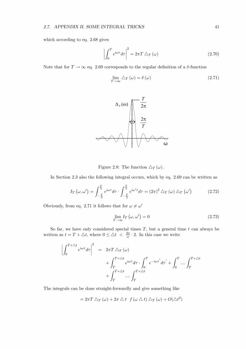
2.7. APPENDIX II. SOME INTEGRAL TRICKS 41
which according to eq. 2.68 gives¯Z T
0eiωτdτ
¯2= 2πT 4T (ω) (2.70)
Note that for T →∞ eq. 2.69 corresponds to the regular definition of a δ-function
limT→∞
4T (ω) = δ (ω) (2.71)
π2T
)(ω∆T
ω
Tπ2
Figure 2.8: The function 4T (ω) .
In Section 2.3 also the following integral occurs, which by eq. 2.69 can be written as
IT¡ω,ω0
¢=
Z T2
−T2
eiωτdτ ·Z T
2
−T2
eiω0τdτ = (2π)24T (ω)4T
¡ω0¢
(2.72)
Obviously, from eq. 2.71 it follows that for ω 6= ω0
limT→∞
IT¡ω,ω0
¢= 0 (2.73)
So far, we have only considered special times T , but a general time t can always bewritten as t = T +4t, where 0 ≤ 4t < 2π
ω · 2. In this case we write¯Z T+4t
0eiωτdτ
¯2= 2πT 4T (ω)
+
Z T+4t
Teiωτdτ ·
Z T
0e−iωτ
0dτ
0+
Z T
0....
Z T+4t
T
+
Z T+4t
T....
Z T+4t
T
The integrals can be done straight-forwardly and give something like
= 2πT 4T (ω) + 2π4 t f (ω4 t)4T (ω) +O(4t2)
42 CHAPTER 2. TIME DEPENDENT PERTURBATION THEORY
where f (ω4 t) oscillates between ±1 as a function of 4t. In the limit of large T (ort), i.e. T À 2π
ω , the first term of this expression is dominant. In other words, a goodapproximation is ¯Z t
0eiωτdτ
¯2≈ 2πt4t (ω)
→ 2πtδ (ω) (2.74)
and at the same time
It¡ω,ω0
¢≈ 0 (2.75)
The function4T (ω) of eq. 2.69 can be examined for fixed T and varying ω. It correspondsthe familiar function found in any book on Fourier transforms
4T (ω) =sin¡ω T2¢
πω(2.76)
The function is shown in Fig. 2.8. It is strongly peaked around ω = 0 and it has zero’s atω = ±2π
T etcetera. The peak’s width at half height is approximately given by
4ω ≈2π
T(2.77)
which gives a measure of the resolution in the ω domain.
Chapter 3
The Quantum Pinball Game
“Degene in balbezit doet iets met de bal”, J. Cruijff over storingstheorie. (“The one in possession
of the ball does something with the ball”, the Dutch philosopher J. Cruijff on perturbation theory.)
Many experiments in which one aims at obtaining quantum information about a sys-tem consists of scattering a beam of microscopic particles of a target and collecting thefragments afterwards. This not only holds for high energy physics with its large accelera-tors and storage rings, but also the spectroscopic experiments of “low energy” molecularand condensed matter physics. Mattuck calls this kind of experiment the quantum pinballgame. In the first section I will explain in more detail what is meant by that. Severalchapters of these lecture notes are concerned with describing quantum pinball games. Wewill use time dependent perturbation theory for that purpose. In view of the complicatedpinball machines presented to us by nature, the first order perturbation term (Fermi’sgolden rule) will often be insufficient to describe what is going on. We need techniquesthat allow us to handle the full perturbation series. An introduction to such techniques isgiven in the second section, which comprises the main part of this chapter. Mattuck givesa discussion in the first chapters of his book, so I will discuss the connection especiallywith his chapter 3. The techniques involve Green functions, a summary of which is givenin the appendix.
3.1 A Typical Experiment
A general template for an experiment is given in Fig. 3.1. A well-prepared beam of micro-scopic particles is send at a target, and the outgoing particles are collected and analyzed inorder to obtain information about the target. An example of such an experiment from con-densed matter physics is electron scattering (or EELS; electron energy loss spectroscopy).The incoming quantum particles are then electrons, usually prepared such that they have
a well-defined momentum p = ~k and energy E = p2
2m . The outgoing particles are also
electrons of which we measure their momenta p0 = ~k0 and energies E0 = p022m . The target
usually is a crystal, which is a quantum many-electron system. Our job is to find outwhat happens inside the target after it has been hit by an incoming particle. This is anexample of a quantum pinball game.
We can play such a game with any kind of particle. For instance, the optical experimentof the previous chapter can be described in terms of: photons in (momentum p = ~k and
43
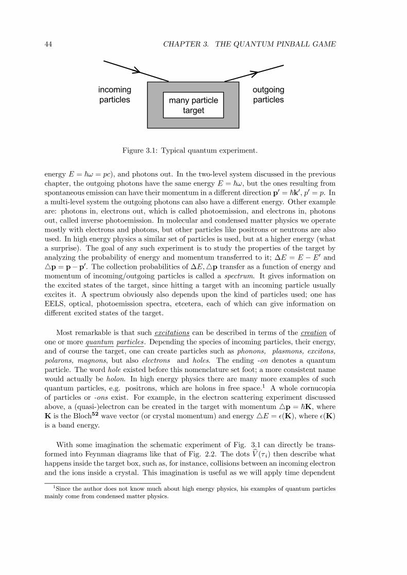
44 CHAPTER 3. THE QUANTUM PINBALL GAME
incomingparticles many particle
target
outgoingparticles
Figure 3.1: Typical quantum experiment.
energy E = ~ω = pc), and photons out. In the two-level system discussed in the previouschapter, the outgoing photons have the same energy E = ~ω, but the ones resulting fromspontaneous emission can have their momentum in a different direction p0 = ~k0, p0 = p. Ina multi-level system the outgoing photons can also have a different energy. Other exampleare: photons in, electrons out, which is called photoemission, and electrons in, photonsout, called inverse photoemission. In molecular and condensed matter physics we operatemostly with electrons and photons, but other particles like positrons or neutrons are alsoused. In high energy physics a similar set of particles is used, but at a higher energy (whata surprise). The goal of any such experiment is to study the properties of the target byanalyzing the probability of energy and momentum transferred to it; ∆E = E − E0 and4p = p−p0. The collection probabilities of ∆E,4p transfer as a function of energy andmomentum of incoming/outgoing particles is called a spectrum. It gives information onthe excited states of the target, since hitting a target with an incoming particle usuallyexcites it. A spectrum obviously also depends upon the kind of particles used; one hasEELS, optical, photoemission spectra, etcetera, each of which can give information ondifferent excited states of the target.
Most remarkable is that such excitations can be described in terms of the creation ofone or more quantum particles. Depending the species of incoming particles, their energy,and of course the target, one can create particles such as phonons, plasmons, excitons,polarons, magnons, but also electrons and holes. The ending -on denotes a quantumparticle. The word hole existed before this nomenclature set foot; a more consistent namewould actually be holon. In high energy physics there are many more examples of suchquantum particles, e.g. positrons, which are holons in free space.1 A whole cornucopiaof particles or -ons exist. For example, in the electron scattering experiment discussedabove, a (quasi-)electron can be created in the target with momentum 4p = ~K, whereK is the Bloch52 wave vector (or crystal momentum) and energy 4E = ²(K), where ²(K)is a band energy.
With some imagination the schematic experiment of Fig. 3.1 can directly be trans-formed into Feynman diagrams like that of Fig. 2.2. The dots bV (τ i) then describe whathappens inside the target box, such as, for instance, collisions between an incoming electronand the ions inside a crystal. This imagination is useful as we will apply time dependent
1Since the author does not know much about high energy physics, his examples of quantum particlesmainly come from condensed matter physics.
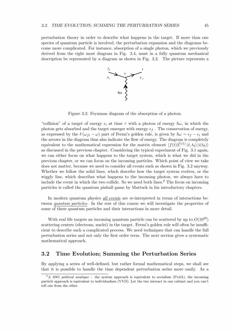
3.2. TIME EVOLUTION; SUMMING THE PERTURBATION SERIES 45
perturbation theory in order to describe what happens in the target. If more than onespecies of quantum particle is involved, the perturbation expansion and the diagrams be-come more complicated. For instance, absorption of a single photon, which we previouslyderived from the right most diagram in Fig. 2.4, must in a fully quantum mechanicaldescription be represented by a diagram as shown in Fig. 3.2. The picture represents a
tτ
0t
iε fε
ω
Figure 3.2: Feynman diagram of the absorption of a photon.
“collision” of a target of energy ²i at time τ with a photon of energy ~ω, in which thephoton gets absorbed and the target emerges with energy ²f . The conservation of energy,as expressed by the δ (ωfi − ω) part of Fermi’s golden rule, is given by ~ω = ²f − ²i andthe arrows in the diagram thus also indicate the flow of energy. The diagram is completelyequivalent to the mathematical expression for the matrix element hf(t)|bU (1) (t, t0) |i(t0)ias discussed in the previous chapter. Considering the typical experiment of Fig. 3.1 again,we can either focus on what happens to the target system, which is what we did in theprevious chapter, or we can focus on the incoming particles. Which point of view we takedoes not matter, because we need to consider all events such as shown in Fig. 3.2 anyway.Whether we follow the solid lines, which describe how the target system evolves, or thewiggly line, which describes what happens to the incoming photon, we always have toinclude the event in which the two collide. So we need both lines.2 The focus on incomingparticles is called the quantum pinball game by Mattuck in his introductory chapters.
In modern quantum physics all events are re-interpreted in terms of interactions be-tween quantum particles . In the rest of this course we will investigate the properties ofsome of these quantum particles and their interactions in more detail.
With real life targets an incoming quantum particle can be scattered by up to O(1023)scattering centers (electrons, nuclei) in the target. Fermi’s golden rule will often be insuffi-cient to describe such a complicated process. We need techniques that can handle the fullperturbation series and not only the first order term. The next section gives a systematicmathematical approach.
3.2 Time Evolution; Summing the Perturbation Series
By applying a series of well-defined, but rather formal mathematical steps, we shall seethat it is possible to handle the time dependent perturbation series more easily. As a
2A 2001 political analoque : the system approach is equivalent to socialism (PvdA), the incomingparticle approach is equivalent to individualism (VVD). Let the two interact in one cabinet and you can’ttell one from the other.
46 CHAPTER 3. THE QUANTUM PINBALL GAME
warning in advance it is fair to say that the formalism not always leads to a simplificationof practical calculations. However, the method will guide our path in the labyrinth ofmany particle physics in the following chapters of these lecture notes. I will use a slightlymore general operator formalism than Mattuck, which has the advantage that you canapply it to any kind of basis set (representation). The spirit of this section however is thesame as Mattuck’s chapter 3. First I will demonstrate the necessary mathematical stepsand then show the connection to Mattuck’s chapter 3.
The central idea to make the time dependent perturbation series easier to handle is toperform the following mathematical steps.
1. Adapt the integration bounds in the time integrals of eq. 2.22 using Green functions.
2. Fourier transform the time integrals to the frequency domain.
3. Sum the perturbation series in the frequency domain.
4. Find a closed expression for the Green function associated with the time evolutionoperator.
More on Green functions can be found in the appendix.We recapitulate the expressions found for the perturbation expansion of the time evo-
lution operator, cf. 2.21 and 2.22
bU (t− t0) = bU0 (t− t0) + ∞Xn=1
bU (n) (t− t0) (3.1)
where
bU (n) (t− t0) =
µ1
i~
¶n Z t
t0
dτn
Z τn
t0
dτn−1.........Z τ2
t0
dτ1
bU0 (t− τn) bV bU0 (τn − τn−1) bV ........bV bU0 (τ1 − t0) (3.2)
We are now restricting ourselves to the case of an time independent perturbation bV andsince bU0 (t− t0) = e− i
~ (t−t0) bH0 (3.3)
where bH0 is also time independent, all the terms in the time evolution operator onlydepend upon the time difference t− t0 and not on the individual times t and t0. Withoutloss of generality, we can choose t0 = 0.We wish to study the situation in which bV is notnecessarily very small, so we expect to be needing a lot of terms in the expansion of eq. 3.1(maybe even an infinite number). Calculating integrals such as eq. 3.2, which contain a lotof oscillating terms such as eq. 3.3 is a nuisance. Those of you who are experienced Fouriertransformers (and you engineers per definition are) know what to do; Fourier transformto the frequency domain. Eq. 3.2 is in fact a multiple convolution integral; the part in τ1for example is Z τ2
0dτ1 bU0 (τ2 − τ1) bV bU0 (τ1) (3.4)
By Fourier transforming a convolution integral in the time domain we will get a productfunction in the frequency domain, which simplifies matters considerably. There is howeverone catch; Fourier integrals usually run from −∞ to +∞.
3.2. TIME EVOLUTION; SUMMING THE PERTURBATION SERIES 47
3.2.1 Adapt Integration Bounds; Green Functions
Luckily it is not a catch-22. Here is the way out; define Green function operators bG+ (t)and bG+0 (t)
i~ bG+ (t) ≡ Θ (t) bU (t) (3.5)
i~ bG+0 (t) ≡ Θ (t) bU0 (t)where Θ (t) is the so-called “theta function” or “step function” which mathematicians alsocall the “Heaviside function”. It is a very peculiar function given by
Θ (t) = 0 t ≤ 0= 1 t > 0 (3.6)
It takes care of what physicists call causality . If we decide to start our system at a timet = 0, then obviously we cannot have evolution before t = 0. Or put in a different way, ifthe cause starts at t = 0, then the effect must be at times t > 0 (this is the definition ofcausality). Causality is expressed by the integration limits of eq. 3.2, where it prescribesthe time order 0 ≤ τ1 ≤ τ2 ≤ ... ≤ τn ≤ t. Using the theta function, causality can beincorporated in a Green function operator. With the help of Green function operators wecan rewrite eq. 3.4, using eq. 3.5, asZ ∞
−∞dτ1 bG+0 (τ2 − τ1) bV bG+0 (τ1) (3.7)
and actually we can rewrite the whole series of time integrals of 3.2 in terms of bG’s andbG0’s with the integrals running from −∞ to +∞ . Note that the theta functions now takecare of the correct time order, cf. eq. 3.6. The factor “i~” in the Green function operatoris just a convention which is used by most authors. The + on bG+ is a “plus” and not a“dagger”; it expresses the fact that this Green function operator differs from zero only forpositive times.
mathematical intermezzo on Green functions
“Verde que the quiero verde. Verde viento. Verde ramas”, Federico Garcia Lorca (Green how I
love you green. Green wind. Green branches).
The operators bG+ and bG+0 are examples of so-called Green function operators.3 Re-member that the operator equation for the time evolution operator, which is equivalentto the Schrodinger equation, is
i~∂
∂tbU (t) = bH bU (t) (3.8)
3I have been told that the correct terminology is Green function and not Green’s function like you findin some textbooks. It is like Fourier transform and Bessel function (and not Fourier’s transform or Bessel’sfunction). Mind you I was educated in Nijmegen, so this could be a catholic convention. In any case,Green functions are named after the English mathematician George Green (1st half 19th century).
48 CHAPTER 3. THE QUANTUM PINBALL GAME
with the initial condition bU (0) = I. From this we can derive an equation for bG+ (t) (seealso Mattuck § 3.4)
i~∂
∂tbG+ (t) =
i~i~
∂
∂tΘ (t) bU (t) = δ (t) bU (t) +Θ (t) ∂
∂tbU (t)
= δ (t) bU (0) + 1
i~Θ (t) bH bU (t) = δ (t) + bH bG+ (t)
or µi~
∂
∂t− bH¶ bG+ (t) = δ (t) (3.9)
In deriving this I have used ∂∂tΘ (t) = δ (t) (see if you can derive this property yourself)
and δ (t) f (t) = δ (t) f (0) (think of an integral with this function).
A general definition of a Green function operator can be given as follows. Let bL be anoperator; then the Green function operator bG(t) belonging to this operator is defined by
bL bG(t) = δ (t) (3.10)
George Green in the 19th century did not know about quantum mechanics of course. Hewas interested in partial differential equations. We can try and make a connection with hisspirit. For example, take one particle in one dimension and write eq. 3.9 in the positionrepresentation as ¿
x
¯µi~
∂
∂t− bH¶ bG+(t)¯x0À =
x|x0® δ (t)⇔Z
dx00¿x
¯i~
∂
∂t− bH ¯x00ÀDx00 ¯ bG+ (t)¯x0E =
x|x0® δ (t)
use the following properties(i) hx|x0i = δ (x− x0)(ii)
x¯i~ ∂
∂t
¯x00®= hx|x00i i~ ∂
∂t ; now use (i)
(iii)Dx¯ bH ¯x00E = hx|x00in− ~2
2m∂2
∂x002 + V (x00)o; as proven in Section 1.3.2, eq. 1.22
(iv)Dx¯ bG+ (t)¯x0E ≡ G+ (x, x0, t)
Using all of this to simplify the equation gives·i~
∂
∂t+~2
2m
∂2
∂x2− V (x)
¸G+
¡x, x0, t
¢= δ
¡x− x0¢ δ (t) (3.11)
The function G+ (x, x0, t) is an example of what a standard mathematician in the field ofdifferential equations would call a Green function. In the formal language of differentialequations, we can state the following. Let L (−→x ) be a differential operator in a set ofvariables −→x = (x1, x2, x3, ......) . Then the Green function is defined as the solution of theequation4
L (−→x )G ¡−→x ,−→x 0¢ = δ¡−→x −−→x 0¢ (3.12)
4δ (−→x −−→x 0) is a short hand notation for δ (x1 − x01)× δ (x2 − x02)× δ (x3 − x03)× ....
3.2. TIME EVOLUTION; SUMMING THE PERTURBATION SERIES 49
You probably have encountered and/or will encounter Green functions anywhere wherepartial differential equations occur and in physics these are not uncommon as you know; thePoisson equation in electrostatics, the wave equation in electrodynamics, the Schrodingerequation in wave mechanics, just to mention a few. Some additional information on Greenfunctions can be found in the appendix. A couple of final remarks on Green functions.
• The Green function does not exist. It is similar to the phrase “Fourier transform”;one should always mention the function of which you want to have the Fouriertransform. Similarly, if you hear the phrase Green function, one should alwaysmention the operator for which you want the Green function. The operator bL (orL (−→x ) in a representation) is defined first and then the Green function is determinedby eq. 3.10 (or eq. 3.12)
• In addition to an operator one should have initial or boundary conditions in orderto fix a Green function operator. For instance, the Green function operator bG+ (t)defined by eqs. 3.5 and 3.9 has bG+ (t) = 0 for t ≤ 0. This is an initial condition inpartial differential equation language. In principle, all sorts of initial and/or bound-ary conditions can be worked into a Green function and each condition leads to aslightly different Green function. Labels like the “+” on bG+ (t) refer to the condi-tions used to construct it. By these labels the Green functions acquire (politicallyincorrect) names like “advanced” or “retarded” Green functions.
3.2.2 Fourier Transform to the Frequency Domain
In terms of the Green function operators defined by eq. 3.5, we can write eqs. 3.1 and 3.2(setting t0 = 0 without loss of generality)
bG+ (t) = bG+0 (t) + ∞Xn=1
bG(n) (t) (3.13)
where
bG(n) (t) =
Z ∞
−∞dτn
Z ∞
−∞......
Z ∞
−∞dτ1
bG+0 (t− τn) bV bG+0 (τn − τn−1) bV ...........bV bG+0 (τ1) (3.14)
We now perform our Fourier transforms. From the convolution theorem we know thatconvolutions in the time domain become simple products in the frequency domain.5 Forinstance, Fourier transforming eq. 3.4 gives
bF (t) = Z ∞
−∞dτ1 bG+0 (τ2 − τ1) bV bG+0 (τ1) FT−→ bF (ω) = bG+0 (ω) bV G+0 (ω) (3.15)
Using the same trick repeatedly in eq. 3.14 gives
bG(n) (ω) = G+0 (ω) bV G+0 (ω) bV .....bV G+0 (ω) (3.16)
5If you have forgotten the convolution theorem, you might want to read Mattuck’s chapter 2 to find aproof.
50 CHAPTER 3. THE QUANTUM PINBALL GAME
and we obtain the equivalent of eq. 3.13 in the frequency domain
bG+ (ω) = bG+0 (ω) + bG+0 (ω) bV bG+0 (ω) + bG+0 (ω) bV bG+0 (ω) bV bG+0 (ω) + .... (3.17)
This is just our perturbation series for the time evolution operator of eq. 3.1 transformedto the frequency domain (using the definition of eq. 3.5)
3.2.3 Sum the Perturbation Series; Dyson Equation
We are now in the position of summing the perturbation series (at least formally). Eq.3.17 can be written as
bG+ (ω) = bG+0 (ω)"I +
∞Xn=1
³bV bG+0 (ω)´n#
(3.18)
The term [...] looks like a simple geometric series likeP∞n=0 r
n = (1−r)−1 which allowsus to write
bG+ (ω) = bG+0 (ω)³I− bV bG+0 (ω)´−1 (3.19)
All the bG’s and bV ’s are operators, so we must keep then in the right order. The −1superscript means “inversion” now; in the following we will show that this is correct.Meanwhile, an equivalent expression is
bG+ (ω) = ³I− bG+0 (ω) bV ´−1 bG+0 (ω) (3.20)
Eq. 3.19 can also be derived formally in a better way by noting that eq. 3.18 is equivalentto
bG+ (ω) = bG+0 (ω) + bG+0 (ω) bV bG+ (ω) (3.21)
Recursion of the right hand side then gives the series of eq. 3.18. Rewriting this as
bG+ (ω)− bG+0 (ω) bV bG+ (ω) = bG+0 (ω)⇔³I− bG+0 (ω) bV ´ bG+ (ω) = bG+0 (ω) (3.22)
then leads to eq. 3.20.
Eq. 3.21 is an important equation called the Dyson equation.6 The Dyson equation isthe equivalent of the whole perturbation series of eqs. 3.1 and 3.2 in the frequency domain.Going back to eq. 3.17 and expanding it as a series is called the Dyson expansion. Eq.3.19 or 3.20 give a formal solution of the Dyson equation which includes all orders n ofthe perturbation bV . We can, if we wish to, now Fourier transform the final result bG+ (ω)back to the time domain and obtain bG+ (t), eq. 3.14, or bU (t), eq. 3.5. Since knowing thetime evolution operator bU (t) is equivalent to solving the Schrodinger equation, the Dyson
6after the english mathematician and theoretical physicist Freeman Dyson (mid 20th century), whoworked with Feynman and Schwinger. In the 2nd world war he also worked as a theoretician for the“bomber command” of the RAF.
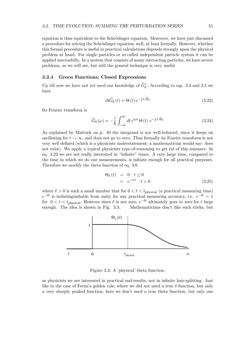
3.2. TIME EVOLUTION; SUMMING THE PERTURBATION SERIES 51
equation is thus equivalent to the Schrodinger equation. Moreover, we have just discusseda procedure for solving the Schrodinger equation; well, at least formally. However, whetherthis formal procedure is useful in practical calculations depends strongly upon the physicalproblem at hand. For single particles or so-called independent particle system it can beapplied successfully. In a system that consists of many interacting particles, we have severeproblems, as we will see, but still the general technique is very useful.
3.2.4 Green Functions; Closed Expressions
Up till now we have not yet used our knowledge of bG+0 . According to eqs. 3.3 and 3.5 wehave
i~ bG0 (t) = Θ (t) e− i~ t.
bH0 (3.23)
Its Fourier transform is
bG0 (ω) = − i~Z ∞
−∞dt eiωtΘ (t) e−
i~ t.
bH0 (3.24)
As explained by Mattuck on p. 40 the integrand is not well-behaved, since it keeps onoscillating for t→∞, and does not go to zero. Thus formally its Fourier transform is notvery well defined (which is a physicists understatement; a mathematician would say: doesnot exist). We apply a typical physicists type-of-reasoning to get rid of this nuisance. Ineq. 3.23 we are not really interested in “infinite” times. A very large time, compared tothe time in which we do our measurements, is infinite enough for all practical purposes.Therefore we modify the theta function of eq. 3.6
Θδ (t) = 0 t ≤ 0= e−δ.t t > 0 (3.25)
where δ > 0 is such a small number that for 0 < t < tphysical (a practical measuring time)e−δt is indistinguishable from unity for any practical measuring accuracy, i.e. e−δt = 1for 0 < t < tphysical. However since δ is not zero, e
−δt ultimately goes to zero for t largeenough. The idea is shown in Fig. 3.3. Mathematicians don’t like such tricks, but
t 0 physicalt ∞
1
)(tδΘ
Figure 3.3: A ‘physical’ theta function.
as physicists we are interested in practical end-results, not in infinite hair-splitting. Justlike in the case of Fermi’s golden rule, where we did not need a true δ-function, but onlya very sharply peaked function, here we don’t need a true theta function, but only one
52 CHAPTER 3. THE QUANTUM PINBALL GAME
which behaves like a theta function over a practical time scale. In practical calculations,we can always choose the parameter δ as small as we like (but not zero). In any case, theintegral of eq. 3.24 becomes well-behaved
bG+0 (ω) = − i~Z ∞
0dt e
i~ (~ω− bH0+iδ)t = ³~ω − bH0 + iδ´−1 (3.26)
Since also the full Hamiltonian bH = bH0 + bV is time independent, we can write bG+ (t) =e−
i~ tbH and similar to bG+0 (ω) we find
bG+ (ω) = ³~ω − bH + iδ´−1
(3.27)
Writing E = ~ω and using units in which ~ = 1, we have bG+ (E) = ³E − bH + iδ
´−1.
Thus we can write
limδ→0
³E − bH´ bG+ (E) = lim
δ→0bG+ (E)³E − bH´ = I (3.28)
So loosely speaking bG+ (E) is the “inverse” of the operator ³E − bH´. By mathematiciansbG+ (E) is also called the resolvent .7We now use a basis set |ni;n = 1, 2..., which consists of eigenstates of the HamiltonianbH|ni = ²n|ni. Applying resolutions of identity to eq. 3.27 it followsbG+ (E) =X
n,m
|nihn| bG+ (E) |mihm| =Xn,m
δn,m|ni (E − ²m + iδ)−1 hm| (3.29)
which gives
bG+ (E) =Xn
|nihn|E − ²n + iδ (3.30)
This way of writing down a Green function operator on the basis of eigenstates of theHamiltonian is very popular. Using the notation of the mathematical intermezzo anddefining φn(x) = hx|ni for wave functions as usual, we have in “wave function” notation
G+¡x, x0, E
¢=Dx¯ bG+ (E)¯x0E =X
n
hx|ni hn|x0iE − ²n + iδ =
Xn
φn(x)φ∗n(x
0)E − ²n + iδ (3.31)
which might be familiar to you from previous encounters with Green functions. Note thatat the points E = ²n, bG+ (E) would go to infinity, if it were not for the convenient iδ term.The inverse of E − bH does not really exist here, that is why we need the iδ to avoid thesepoints.8 Fourier transforming this expression to the time domain (using complex contourintegration, see the appendix of the next chapter) gives the expression
G+¡x, x0, t
¢=Xn
φn(x)φ∗n(x
0) e−i²ntΘ(t) (3.32)
7Whether they really think it resolves all our problems I don’t know.8In the terminology of complex function theory we say that bG+ (E) has a “pole”at E = ²n for δ → 0,
or a “pole” at E = ²n − iδ in the complex plane, which becomes real for δ → 0. See the appendix of thenext chapter.
3.2. TIME EVOLUTION; SUMMING THE PERTURBATION SERIES 53
From the expression of the Green function operator of eq. 3.27 we can also recover theDyson equation of eq. 3.21.
bG+ (E) = ³E − bH + iδ´− 1
=³E − bH0 + iδ − bV ´−1 = ³ bG+−10 (E)− bV ´−1 (3.33)
or, in other words ³ bG+−10 (E)− bV ´ bG+ (E) = I (3.34)
or bG+0 (E)³ bG+−10 (E)− bV ´ bG+ (E) = bG+0 (E)⇐⇒
³I− bG+0 (E) bV ´ bG+ (E) = bG+0 (E) (3.35)
which can be rewritten as bG+ (E) = bG+0 (E) + bG+0 (E) bV bG+ (E) (3.36)
which is the Dyson equation again.
3.2.5 Summary
In case you don’t see the wood for the trees anymore, here is a short summary of theprevious sections. We have a HamiltonianbH = bH0 + bV (3.37)
where bH0 describes an “unperturbed” system and bV is a “perturbation”. We can writethe time-evolution operator of the perturbed system, described by the full Hamiltonian as
bU (t) = e− i~ tbH = e− i
~ tbH0 + ∞X
n=1
µ1
i~
¶n Z t
0dτn
Z τn
0dτn−1.......
Z τ2
0dτ1
e−i~ (t−τn) bH0 bV e− i
~ (τn−τn−1) bH0 bV .......e− i~ τ1 bH0 (3.38)
This expression can be simplified in a series of steps.
1. Define a Green function operator by
i~ bG+ (t) = Θδ (t) bU (t) (3.39)
We can prove³i~ ∂
∂t − bH´ bG+ (t− t0) = δ (t− t0), which makes it a “Green functionoperator” in the mathematical sense.
2. Using the definition 3.39 in 3.38 and Fourier transforming to the frequency domainwe get the series
bG+ (ω) = bG+0 (ω) + bG+0 (ω) ∞Xn=1
³bV bG+0 (ω)´n = bG+0 (ω) + bG+0 (ω) bV bG+ (ω) (3.40)
54 CHAPTER 3. THE QUANTUM PINBALL GAME
which is also called the Dyson equation.
3 Eq.3.40 can be “solved” formally as
bG+ (ω) = ³I− bG+0 (ω) bV ´−1 bG+0 (ω) (3.41)
4 which can also be shown to be identical to the resolvent operator
bG+ (ω) = ³~ω − bH + iδ´−1
(3.42)
Usually the expression of step 4 is only useful in formal manipulations, but not in practicalcalculations. Note for instance that the expression of eq. 3.30 assumes that we know allthe eigenstates of the full Hamiltonian; if we did, we wouldn’t have any problems to startwith. Whether the expression of step 3 is useful in practical calculations depends uponhow difficult it is to calculate the inverse, i.e. (....)−1; for single or independent particlesit can be done. If it proves to be too difficult, we have to solve Dyson’s equation in step2 via another route. More of this in Chapter 4.
3.3 Connection to Mattuck’s Ch. 3
Mattuck starts his pinball game simple with just a single electron. The scattering poten-tials in his pinball machine are the ion cores or nuclei in a crystal. The properties of hissingle electron pinball are summarized in his table 3.1. This table is equivalent to ourtime dependent perturbation series of eqs. 2.21 and 2.22 and Figs. 2.2 and 2.3. Mattuckgives sort of a description of the foregoing formalism in his chapter 3, which I advice youto read after this point. I will explicitly describe the connection with the present chapter.Mattuck’s eq. 3.1 on p.38 gives the general many particle definition of a (one-particle)propagator; the rest of chapter 3 just deals with the specific case of a single particle.Suppose |r1i is an eigenstate of the position generator
br|r1i = r1|r1i (3.43)
At t = t1 we start with a particle in this particular state |r1(t1)i.We let the particle evolve(propagate) under the full Hamiltonian to t2 and ask for the probability amplitude to findit in |r2(t2)i, or in other words to find it at position r2. The probability amplitude is givenby D
r2(t2)¯ bU (t2 − t1)¯ r1(t1)E t2 > t1 (3.44)
This is identical to Mattuck’s definition of his “propagator” of eq. 3.1, iG+ (r2, r1, t2 − t1)Actually, we could have used our definition of bG+ (t2 − t1) in eq. 3.44, which for t2 > t1is identical to bU (t2 − t1). In other words Mattuck’s eq. 3.1 is just the position represen-tation of our Green function operator. Mattuck’s eq. 3.2 on p. 39 is simply a matrixrepresentation of the same Green function operator using another basis set. The example
3.4. APPENDIX. GREEN FUNCTIONS; THE LIPPMANN-SCHWINGER EQUATION55
Mattuck worked in detail has bH = bH0 + bV , where bH0 = bp22m is the Hamiltonian of a “free
particle”. The eigenstates of the latter are also the eigenstates of the momentum operatorbp|pi = p|pibH0|pi = ²p|pi ²p =
p2
2m(3.45)
In wave function notation we can write
hr|pi ≡ φp (r) ∝ ei~ p·r (3.46)
as we have seen in one of the exercises. Using this set of eigenstates we get, in the“momentum representation”D
p0¯ bG+0 (t2 − t1)¯pE = δ
¡p0 − p¢Θ (t2 − t1) e− i
~ ²p(t2−t1) ≡ δ¡p0 − p¢G+0 (p, t2 − t1)
(3.47)
which corresponds to Mattuck’s eq. 3.9 on p. 40. In the example of § 3.2, p. 43 Mattuckuses a “perturbation” of the form V (bp) where
p0 |V (bp)|p® = δ¡p0 − p¢V (p) (3.48)
in the momentum representation. The time evolution operator of eq. 3.38 can be trans-formed into the momentum representation by inserting a resolution of identity I =
Rdp |pihp|
between each pair of operators. The result becomes simple, since in all matrices only thediagonal terms survive, by virtue of eqs. 3.47 and 3.48. The final results are Mattuck’seqs. 3.30 and 3.31. Mattuck’s §3.3 and 3.4 describe the same mathematical steps wehave performed for our Green function, but now for this special case in the momentumrepresentation.
3.4 Appendix. Green Functions; the Lippmann-SchwingerEquation
What use is a Green function ? This question has haunted many generations ofphysics students. A popular story on the origin of “Green functions” states that, whenevera a theorist mentions the word Green function, all experimentalists get dizzy and green inthe face, and have to leave the room.9 The followers of George Green, who gave his nameto these functions, were interested in solving differential equations of the form
L (−→x )φ (−→x ) = ρ (−→x ) (3.49)
where L (−→x ) is some differential operator, ρ (−→x ) is a fixed function called the source, andφ (−→x ) is the solution of the equation we are after. For instance from electrostatics weknow the Poisson equation
∇2φ (r) = 4πρ (r) (3.50)
9I don’t think this story is entirely true. Some of them become red in the face and very agitated,...before they leave the room.
56 CHAPTER 3. THE QUANTUM PINBALL GAME
The source ρ (r) is the charge density, which we assume to be given, and φ (r) is theelectrostatic potential, which we want to determine. Suppose we know the solution to theequation
∇2G ¡r, r0¢ = δ¡r− r0¢ (3.51)
which defines a Green function a la George Green. The solution to the Poisson equationcan then be written as
φ (r) = φ0 (r) + 4π
ZG¡r, r0
¢ρ¡r0¢d3r0 (3.52)
where φ0 (r) is a general solution of the homogeneous equation ∇2φ0 (r) = 0 (the Laplaceequation). Substituting eq. 3.52 in eq. 3.50 one easily proves that this is the solution. Wehave “solved” the Poisson equation in two steps. The differential operator part is takencare of by defining a Green function as in eq. 3.51 and then the source term ρ (r) partis incorporated by applying eq. 3.52. The differential equation part, eq. 3.51, is solvedfirst, subject to the relevant boundary conditions (in electrostatics boundary conditionsare usually determined by the presence of conducting or dielectric objects). Here is thecrux: once we have obtained the Green function,10 we can calculate the potential for anycharge density ρ (r) simply by applying eq. 3.52.
The Poisson equation is inhomogeneous, i.e. it can be expressed like eq. 3.49 witha non-zero source term. The Schrodinger equation is homogeneous, i.e. it has the formL (−→x )φ (−→x ) = 0. Let us take the simple one-dimensional example from wave mechanicsagain. The two variables are −→x = (x, t) and the Schrodinger equation is½
i~∂
∂t+~2
2m
∂2
∂x2− V (x)
¾φ (x, t) = 0 (3.53)
How can we apply Green magic to a homogeneous equation like the Schrodinger equationin the same way as above ? Well, by using a trick. We rewrite the Schrodinger equationas ½
i~∂
∂t+~2
2m
∂2
∂x2
¾φ (x, t) = V (x)φ (x, t) (3.54)
and we treat the right hand side as a source term (even though formally this is not true,since it contains the solution we are after, rather than being a fixed function like in thePoisson equation). The rest is on automatic pilot. First we obtain a Green function bysolving ½
i~∂
∂t+~2
2m
∂2
∂x2
¾G+0
¡x, t;x0, t0
¢= δ
¡x− x0¢ δ ¡t− t0¢ (3.55)
and then, in analogy to the Poisson case, the solution to eq. 3.54 can be written as
φ (x, t) = φ0 (x, t) +
ZZG+0
¡x, t;x0, t0
¢V (x0)φ
¡x0, t0
¢dx0 dt0 (3.56)
10How this is done can be found in Electricity & Magnetism books, e.g. J. D. Jackson, ClassicalElectrodynamics, (Wiley, New York, 1975).
3.4. APPENDIX. GREEN FUNCTIONS; THE LIPPMANN-SCHWINGER EQUATION57
where φ0 (x, t) is a general solution of the homogeneous equation½i~
∂
∂t+~2
2m
∂2
∂x2
¾φ0 (x, t) = 0
Actually this part is easy. The solution of the homogeneous equation is a simple planewave.
φ0,k (x, t) =
r1
2πei(kx−ωt) with ~ω =
(~k)2
2m
The Green function G+0 (x, t, x0, t0) can then be calculated from eq. 3.32 noting that the
continuous index k labels the eigenstates.11
G+0 (x, t, x0, t0) =
Zdk φ0,k (x, 0)φ0,k
¡x0, 0
¢e−
i~(~k)22m
(t−t0)Θ(t− t0)
=
µ −mi2π~(t− t0)
¶12
exp
Ã−m |x− x
0|22i~(t− t0)
!Θ(t− t0) (3.57)
The Green function incorporates causality, i.e. t > t0. By direct substitution in eq. 3.55one can see that this is a solution. There are a couple of snakes in the grass. First andforemost, eq. 3.56 is not a solution to the problem, since it contains the unknown functionφ (x, t) on the right-hand side as well as on the left-hand side. Instead, it is an integralequation from which φ (x, t) has to be solved. This is different from an inhomogeneousequation like the Poisson equation where eq. 3.52 directly gives you the solution. In theway we have derived eq. 3.56 you can easily see that it must be completely equivalent tothe Schrodinger equation.
The integral equation of eq. 3.56 is called the Lippmann08-Schwinger65 equation. Isit easier to solve than the Schrodinger (differential) equation? That depends upon thephysical problem at hand. The Lippmann-Schwinger equation is used a lot in “scatter-ing theory” in which the scattering of quantum particles (by fixed targets and/or otherparticles) is studied. There is also a Lippmann-Schwinger equation in electromagnetismwhere propagation of electromagnetic waves is studied. It is also used in studying thepropagation of acoustical and seismological waves, so it is a versatile technique.
What does this have to do with the Green functions we encountered in the main text?First of all, there is a good reason for the notation G+0 for the Green function in eq. 3.56.One just has to follow the reasoning which lead to eq. 3.11 backwards to see that it canbe written as
G+0¡x, t;x0, t0
¢=Dx¯ bG+0 ¡t− t0¢¯x0E = 1
i
Dx¯e−
i~ (t−t0) bH0 ¯x0EΘ(t− t0) (3.58)
We now recognize eq. 3.56 as the position representation of the general form of theLippmann-Schwinger equation
|φ(t)i = |φ0(t)i+Z bG+0 ¡t− t0¢ bV |φ(t0)i dt0 (3.59)
11More on analytical expressions of Green functions for a number of (simple) cases can be found inmathematical physics books, e.g. P. R. Wallace, Mathematical Analysis of Physical Problems, (Dover, NewYork, 1984).
58 CHAPTER 3. THE QUANTUM PINBALL GAME
(remember hx|φ(t)i = φ (x, t) andDx¯ bV ¯x0E = V (x)δ(x− x0) ). Now let us write |φ(t)i =bU (t− t0) |φ(t0)i = 1
ibG+ (t− t0) |φ(t0)i for the formal time evolution of the state with
respect to an arbitrary starting point t0 as we did before. Eq. 3.59 becomes, dropping the1i at the right and left hand sides
bG+ (t− t0) |φ(t0)i = bG+0 (t− t0) |φ0(t0)i+½Z bG+0 ¡t− t0¢ bV bG+ ¡t0 − t0¢ dt0¾ |φ(t0)i(3.60)
Now there is one last trick. Consider the typical scattering experiment of Fig. 3.1. At thestarting time t0, just when the incoming particles start to leave their source, they are farfrom the target. At that point in time they do not yet experience the perturbing potentialV which originates from the target. In other words, they still behave like free particles,which means at time t0 we have |φ(t0)i = |φ0(t0)i. But then eq. 3.60, which must beobeyed for any starting condition |φ0(t0)i, becomes an equation for the operator
bG+ (t− t0) = bG+0 (t− t0) + Z bG+0 ¡t− t0¢ bV bG+ ¡t0 − t0¢ dt0 (3.61)
If one Fourier transforms this equation to the frequency domain, one immediately rec-ognizes the Dyson equation, eq. 3.21. This means that one can tackle the Lippmann-Schwinger equation of eq. 3.56 using the Green function techniques (Dyson equation,summation of perturbation series, etcetera) discussed in this chapter.
In the Born approximation, eq. 2.23, one only includes the perturbation in first order.This corresponds to using bG+0 ’s only on the right hand side of eq. 3.61. Working our waybackwards to eqs. 3.59 and 3.56 one easily sees that the Born approximation correspondsto using φ0 (x, t)’s only on the right hand side of the Lippmann-Schwinger equation.
φ (x, t) = φ0 (x, t) +
ZZG+0
¡x, t;x0, t0
¢V (x0)φ0
¡x0, t0
¢dx0 dt0
In the Born approximation the equation becomes of the same type as eq. 3.52, i.e. theunknown φ (x, t) only occurs on the left hand side, and can thus be calculated straightfor-wardly. Because of its simplicity, the Born approximation is used quite a lot in scatteringcalculations, or more generally, in studying the scattering and propagation of all sorts ofwaves. It is even used in situations where the perturbation is not really small enough inorder to justify using it only in first order. But, as often in practical physics, one stretchesthe limit.
In summary: what use are Green functions ?
• They provide a general approach for solving an inhomogeneous partial differentialequation, see eqs. 3.49—3.52.
• For a homogeneous partial differential equation they provide an alternative: anintegral (Lippmann-Schwinger) equation. This can be approached using the Greenfunction techniques (Dyson equation, summation of perturbation series) discussedin this chapter.
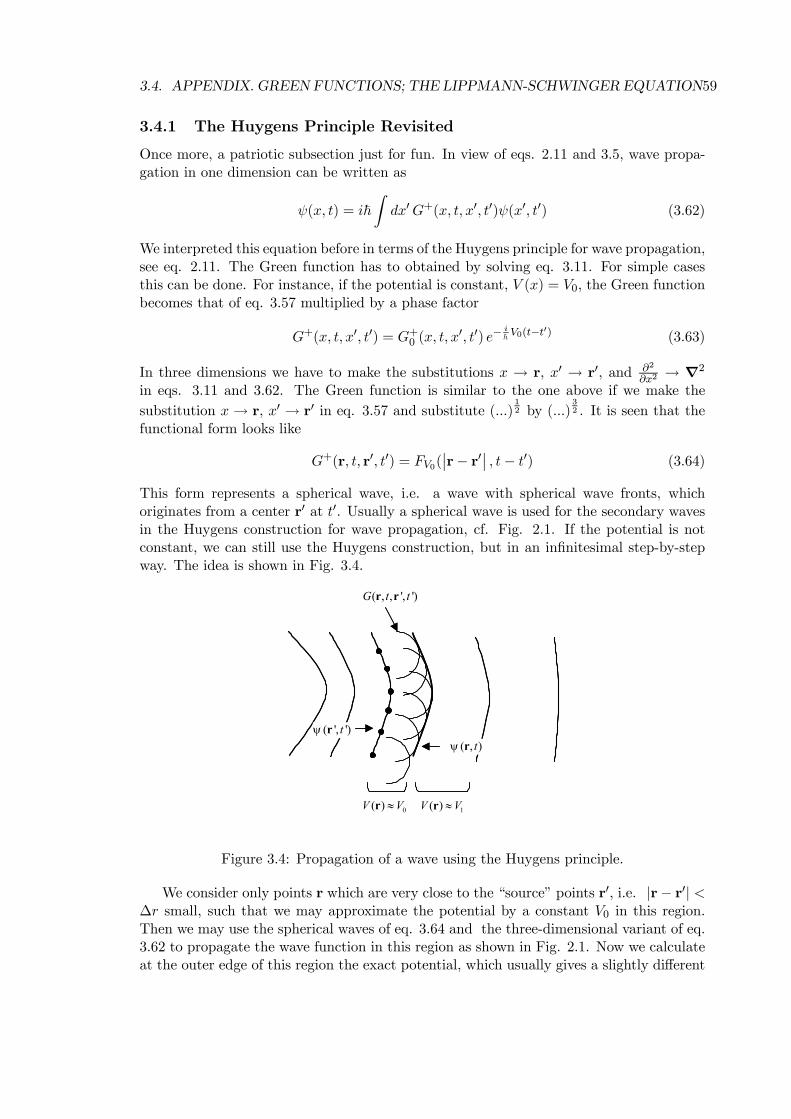
3.4. APPENDIX. GREEN FUNCTIONS; THE LIPPMANN-SCHWINGER EQUATION59
3.4.1 The Huygens Principle Revisited
Once more, a patriotic subsection just for fun. In view of eqs. 2.11 and 3.5, wave propa-gation in one dimension can be written as
ψ(x, t) = i~Zdx0G+(x, t, x0, t0)ψ(x0, t0) (3.62)
We interpreted this equation before in terms of the Huygens principle for wave propagation,see eq. 2.11. The Green function has to obtained by solving eq. 3.11. For simple casesthis can be done. For instance, if the potential is constant, V (x) = V0, the Green functionbecomes that of eq. 3.57 multiplied by a phase factor
G+(x, t, x0, t0) = G+0 (x, t, x0, t0) e−
i~ V0(t−t0) (3.63)
In three dimensions we have to make the substitutions x → r, x0 → r0, and ∂2
∂x2→ ∇2
in eqs. 3.11 and 3.62. The Green function is similar to the one above if we make the
substitution x → r, x0 → r0 in eq. 3.57 and substitute (...)12 by (...)
32 . It is seen that the
functional form looks like
G+(r, t, r0, t0) = FV0(¯r− r0¯ , t− t0) (3.64)
This form represents a spherical wave, i.e. a wave with spherical wave fronts, whichoriginates from a center r0 at t0. Usually a spherical wave is used for the secondary wavesin the Huygens construction for wave propagation, cf. Fig. 2.1. If the potential is notconstant, we can still use the Huygens construction, but in an infinitesimal step-by-stepway. The idea is shown in Fig. 3.4.
( ', ')tψ r
( , , ', ')G t tr r
( , )tψ r
0( )V V≈r 1( )V V≈r
( ', ')tψ r
( , , ', ')G t tr r
( , )tψ r
0( )V V≈r 1( )V V≈r
Figure 3.4: Propagation of a wave using the Huygens principle.
We consider only points r which are very close to the “source” points r0, i.e. |r− r0| <∆r small, such that we may approximate the potential by a constant V0 in this region.Then we may use the spherical waves of eq. 3.64 and the three-dimensional variant of eq.3.62 to propagate the wave function in this region as shown in Fig. 2.1. Now we calculateat the outer edge of this region the exact potential, which usually gives a slightly different
60 CHAPTER 3. THE QUANTUM PINBALL GAME
value V1. We approximate in an adjacent region the potential by this new constant V1.We still can use spherical waves to propagate the wave in this new region, but we haveto recalculate it using eq. 3.63 with V1 instead of V0. We can now propagate our wavethrough the next small step ∆r,∆t in space and time. Using this procedure iterativelywe can propagate our wave throughout the whole space and time. Fig. 3.4 is again alittle bit misleading is the sense that a spherical wave should emerge from each point r0
in space, and the wave function ψ(r, t) should be constructed from the interference of allsuch waves.
The beauty of it all is that Huygens got his idea in 1678, before anything was knownabout Green functions, or indeed anything was known about wave equations. Huygensonly used his intuition. Personally I feel that “Green functions” should be called “Huygensfunctions”. Almost three centuries later, in 1948, Richard Feynman was again inspiredby Huygens’s idea, which he implemented in his famous path integral method for solvingwave equations.12
12R. P. Feynman, Space-Time Approach to Non-Relativistic Quantum Mechanics, Rev. Mod. Phys. 20,367 (1948).
Chapter 4
Scattering
Scattering theory is an very broad subject. It is used to describe scattering phenomena ina wide range of fields in physics, from the collisions of elementary particles to the motionof seismic waves through the earth’s interior. Naturally our discussion will mainly bewithin the context of quantum mechanics, and more specifically within the context ofthe quantum pinball game or the typical experiment of Fig. 3.1. Even here we have torestrict ourselves severely. We will only consider the scattering of a single particle by acollection of fixed scattering centers which we are far apart, a so-called “dilute sample”.The classical example is scattering of α-particles through a thin gold foil, which was usedby Rutherford08 to demonstrate the existence of a massive, but small nucleus inside theatoms. Other examples are the motion of a quantum particle (e.g. an electron) throughan atomic gas; or the motion of an electron through an ideal metal containing impurityions in a dilute concentration. These are examples of a quantum pinball game as explainedin the previous chapter. The outgoing particle is the same as the incoming particle andthe “pinball machine” contains no other particles, only fixed scattering centers. Even thisproblem we will at not consider in its full detail. In principle the outgoing particle canbe in a different quantum state than the incoming particle. We will only consider elasticscattering, i.e. the energy of the incoming and outgoing particle is the same. Furthermorewe assume that the scattering potential cannot change the spin state of the incomingparticle, so we do not have to consider spin explicitly. There are many cases for which theseassumptions are very reasonable. Consider scattering of electrons by atoms, for instance.Atoms are much heavier than electrons, so in an elastic collision the energy transfer fromelectrons to atoms is indeed very small. In an inelastic scattering the electron excites theatom; such processes do happen, but we won’t consider them here.1 Furthermore, fornot too heavy atoms (all but the bottom rows of the periodic table) the spin state of anelectron is indeed unchanged in a collision. In summary, we will be looking at the casein which only the direction of the momentum p0 of the outgoing particle can differ fromthat of the incoming particle p, whereas the size (which is given by the energy ² = p2
2m)remains the same, i.e. |p| = |p0|.
First I will give a general introduction to the scattering of waves, which, although wewill use electron waves as an example, is not very specific to quantum mechanics perse.This is mainly to show that the most important measurable quantities can all be derivedfrom the so-called scattering amplitudes. The size and phase of these amplitudes are char-
1The general formalism discussed here can be extended in a straight-forward way to include inelasticprocesses. The notation becomes a bit messy however, which is why I skipped it.
61
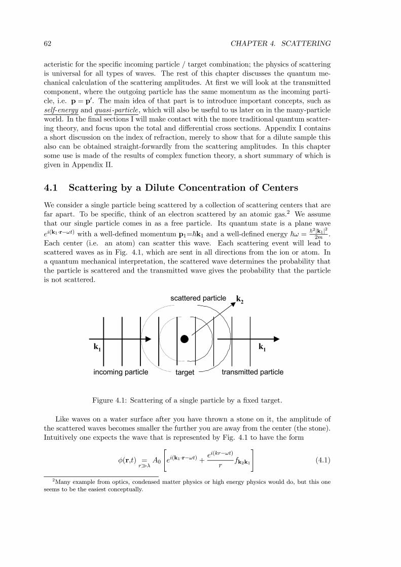
62 CHAPTER 4. SCATTERING
acteristic for the specific incoming particle / target combination; the physics of scatteringis universal for all types of waves. The rest of this chapter discusses the quantum me-chanical calculation of the scattering amplitudes. At first we will look at the transmittedcomponent, where the outgoing particle has the same momentum as the incoming parti-cle, i.e. p = p0. The main idea of that part is to introduce important concepts, such asself-energy and quasi-particle, which will also be useful to us later on in the many-particleworld. In the final sections I will make contact with the more traditional quantum scatter-ing theory, and focus upon the total and differential cross sections. Appendix I containsa short discussion on the index of refraction, merely to show that for a dilute sample thisalso can be obtained straight-forwardly from the scattering amplitudes. In this chaptersome use is made of the results of complex function theory, a short summary of which isgiven in Appendix II.
4.1 Scattering by a Dilute Concentration of Centers
We consider a single particle being scattered by a collection of scattering centers that arefar apart. To be specific, think of an electron scattered by an atomic gas.2 We assumethat our single particle comes in as a free particle. Its quantum state is a plane wave
ei(k1·r−ωt) with a well-defined momentum p1=~k1 and a well-defined energy ~ω = ~2|k1|22m .
Each center (i.e. an atom) can scatter this wave. Each scattering event will lead toscattered waves as in Fig. 4.1, which are sent in all directions from the ion or atom. Ina quantum mechanical interpretation, the scattered wave determines the probability thatthe particle is scattered and the transmitted wave gives the probability that the particleis not scattered.
k1
incoming particle transmitted particle
scattered particle
k1
k2
target
Figure 4.1: Scattering of a single particle by a fixed target.
Like waves on a water surface after you have thrown a stone on it, the amplitude ofthe scattered waves becomes smaller the further you are away from the center (the stone).Intuitively one expects the wave that is represented by Fig. 4.1 to have the form
φ(r,t) =rÀλ
A0
"ei(k1·r−ωt) +
ei(kr−ωt)
rfk2k1
#(4.1)
2Many example from optics, condensed matter physics or high energy physics would do, but this oneseems to be the easiest conceptually.
4.1. SCATTERING BY A DILUTE CONCENTRATION OF CENTERS 63
at a large distance from the target (distance measured in units of wave length). The firstterm on the right hand side describes an incoming plane wave. The “intensity” of theincoming wave is3
Iin =¯A0e
i(k1·r−ωt)¯2= |A0|2 (4.2)
The second term on the right hand side of eq. 4.1 describes the outgoing scattered wave. Inan isotropic medium far from the target, scattered waves always have spherical wave fronts,irrespective of the “shape” of the target. Note that we may write k = |k1| = |k2|; in elasticscattering the wave number does not change. The amplitude A of the outgoing sphericalwave goes as A(r) ∝ 1/r, where r is the distance to the center. The total intensity (or inquantum mechanical terms the total probability) has to be distributed over the surface ofa sphere of radius r, and since the total must be constant, the local intensity (probability,which is A2) goes as 1/r2. The amplitude of the outgoing spherical wave in generaldepends upon the direction k2 with respect to that of the incoming wave k1. This angulardependence is represented by the scattering factors fk2k1 in eq. 4.1. The fk2k1 are calledthe scattering amplitudes. In general these will be complex numbers, so they have a phaseas well as an amplitude. They contains all the target specific information.
Once we know how a single microscopic target scatters the incoming particles, we cantry and figure out how a real macroscopic sample used in an experiment behaves. Amacroscopic sample consists of many microscopic targets (atoms) and spherical scatteredwaves emerge from all these targets. How the sample as a whole scatters depends verymuch upon the conditions of the experiment. Suppose we can divide our system into cubicboxes of size L (volume Ω = L3) such that each box contains one target and the probabilityof finding two targets in one box is negligible. If nI is the density of the gas, then simplyΩ = 1/nI . If we are not near a thermodynamic critical point, density fluctuations aresmall, so the probability of finding more than (or less than) one target per Ω is indeedvery small. The basic idea is shown in Fig. 4.2.
In particle scattering the conditions are usually quite different from what you mightknow from diffraction. We have stated that our source produces incoming particles ofwell-defined energy and momentum such that its quantum state can be represented by aplane wave ei(k1·r−ωt). This is of course an idealization; a real source usually produces anincoherent beam of particles. In wave terms, an incoherent beam consists of a series ofpulses, so-called wave packets. Each wave packet has a size ` that is sufficiently long, sothat the packet is nearly monochromatic, i.e. nearly a wave with a well-defined frequency(energy) and wave length (momentum). ` is called the coherence length, divided by thewave’s speed v = p/m = ~k1/m it gives the coherence time τ c = `/v. Obviously one musthave `À λ for a nearly monochromatic wave. There is however no phase relation between
3A “proper intensity” should have the dimension£W/m2
¤, whereas the “intensity” given here has the
dimension of a “particle density”£1/m3
¤(¯φ(r,t)2
¯d3r gives the probability of finding a particle in a volume
d3r, so the dimension of£¯φ(r,t)2
¯¤=£1/m3
¤). Multiplying the particle density
¯φ2¯by the speed v of
the particles gives the “flux” of particles v¯φ2¯, i.e. the number of particles crossing a unit surface per
unit time. Multiplying this with the energy ~ω per particle gives the “proper intensity” ~ωv¯φ2¯, which
has the required dimension£J/(sm2)
¤. Since v and ω are constants here, and we normalize with respect
to the incoming beam anyway, the concepts “particle density”, “flux”, “proper intensity” can all be usedto represent “intensity”. Here we use “particle density” because it is the easiest. In quantum scatteringtheory one frequently uses “flux”; in scattering of electromagnetic or acoustic waves one normally uses the“proper intensity”.
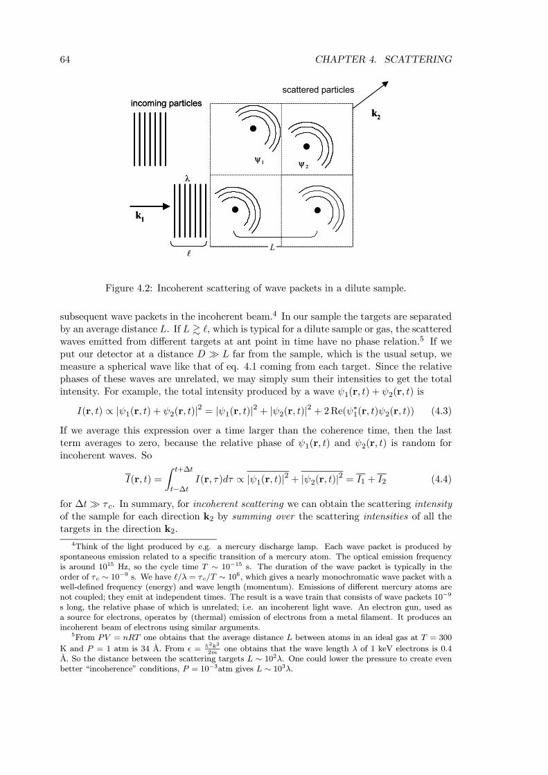
64 CHAPTER 4. SCATTERING
incoming particlesscattered particles
L
λ
1ψ2ψ
k2
k1
incoming particlesscattered particles
L
λ
1ψ2ψ
k2
k1
Figure 4.2: Incoherent scattering of wave packets in a dilute sample.
subsequent wave packets in the incoherent beam.4 In our sample the targets are separatedby an average distance L. If L & `, which is typical for a dilute sample or gas, the scatteredwaves emitted from different targets at ant point in time have no phase relation.5 If weput our detector at a distance D À L far from the sample, which is the usual setup, wemeasure a spherical wave like that of eq. 4.1 coming from each target. Since the relativephases of these waves are unrelated, we may simply sum their intensities to get the totalintensity. For example, the total intensity produced by a wave ψ1(r, t) + ψ2(r, t) is
I(r, t) ∝ |ψ1(r, t) + ψ2(r, t)|2 = |ψ1(r, t)|2 + |ψ2(r, t)|2 + 2Re(ψ∗1(r, t)ψ2(r, t)) (4.3)
If we average this expression over a time larger than the coherence time, then the lastterm averages to zero, because the relative phase of ψ1(r, t) and ψ2(r, t) is random forincoherent waves. So
I(r, t) =
Z t+∆t
t−∆tI(r, τ)dτ ∝ |ψ1(r, t)|2 + |ψ2(r, t)|2 = I1 + I2 (4.4)
for ∆tÀ τ c. In summary, for incoherent scattering we can obtain the scattering intensityof the sample for each direction k2 by summing over the scattering intensities of all thetargets in the direction k2.
4Think of the light produced by e.g. a mercury discharge lamp. Each wave packet is produced byspontaneous emission related to a specific transition of a mercury atom. The optical emission frequencyis around 1015 Hz, so the cycle time T ∼ 10−15 s. The duration of the wave packet is typically in theorder of τc ∼ 10−9 s. We have `/λ = τc/T ∼ 106, which gives a nearly monochromatic wave packet with awell-defined frequency (energy) and wave length (momentum). Emissions of different mercury atoms arenot coupled; they emit at independent times. The result is a wave train that consists of wave packets 10−9
s long, the relative phase of which is unrelated; i.e. an incoherent light wave. An electron gun, used asa source for electrons, operates by (thermal) emission of electrons from a metal filament. It produces anincoherent beam of electrons using similar arguments.
5From PV = nRT one obtains that the average distance L between atoms in an ideal gas at T = 300
K and P = 1 atm is 34 A. From ² = ~2k22m
one obtains that the wave length λ of 1 keV electrons is 0.4A. So the distance between the scattering targets L ∼ 102λ. One could lower the pressure to create evenbetter “incoherence” conditions, P = 10−3atm gives L ∼ 103λ.
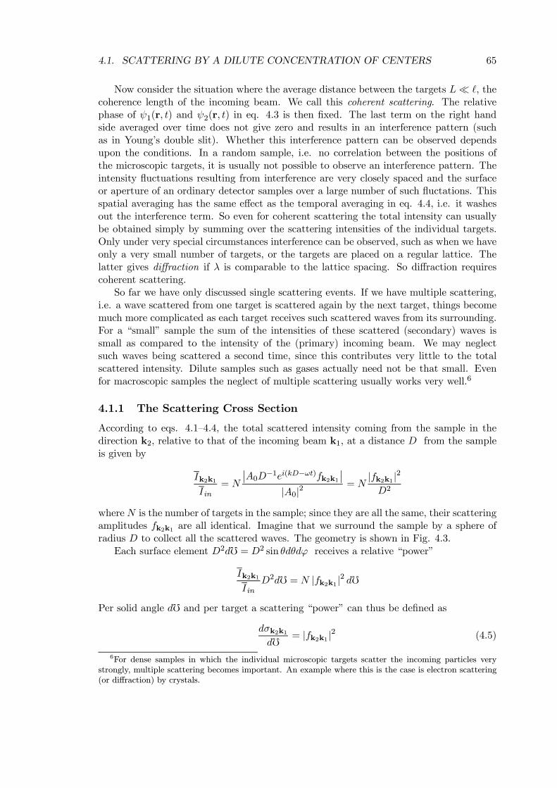
4.1. SCATTERING BY A DILUTE CONCENTRATION OF CENTERS 65
Now consider the situation where the average distance between the targets L¿ `, thecoherence length of the incoming beam. We call this coherent scattering. The relativephase of ψ1(r, t) and ψ2(r, t) in eq. 4.3 is then fixed. The last term on the right handside averaged over time does not give zero and results in an interference pattern (suchas in Young’s double slit). Whether this interference pattern can be observed dependsupon the conditions. In a random sample, i.e. no correlation between the positions ofthe microscopic targets, it is usually not possible to observe an interference pattern. Theintensity fluctuations resulting from interference are very closely spaced and the surfaceor aperture of an ordinary detector samples over a large number of such fluctations. Thisspatial averaging has the same effect as the temporal averaging in eq. 4.4, i.e. it washesout the interference term. So even for coherent scattering the total intensity can usuallybe obtained simply by summing over the scattering intensities of the individual targets.Only under very special circumstances interference can be observed, such as when we haveonly a very small number of targets, or the targets are placed on a regular lattice. Thelatter gives diffraction if λ is comparable to the lattice spacing. So diffraction requirescoherent scattering.
So far we have only discussed single scattering events. If we have multiple scattering,i.e. a wave scattered from one target is scattered again by the next target, things becomemuch more complicated as each target receives such scattered waves from its surrounding.For a “small” sample the sum of the intensities of these scattered (secondary) waves issmall as compared to the intensity of the (primary) incoming beam. We may neglectsuch waves being scattered a second time, since this contributes very little to the totalscattered intensity. Dilute samples such as gases actually need not be that small. Evenfor macroscopic samples the neglect of multiple scattering usually works very well.6
4.1.1 The Scattering Cross Section
According to eqs. 4.1—4.4, the total scattered intensity coming from the sample in thedirection k2, relative to that of the incoming beam k1, at a distance D from the sampleis given by
Ik2k1Iin
= N
¯A0D
−1ei(kD−ωt)fk2k1¯
|A0|2= N
|fk2k1 |2D2
whereN is the number of targets in the sample; since they are all the same, their scatteringamplitudes fk2k1 are all identical. Imagine that we surround the sample by a sphere ofradius D to collect all the scattered waves. The geometry is shown in Fig. 4.3.
Each surface element D2df = D2 sin θdθdϕ receives a relative “power”
Ik2k1Iin
D2df = N |fk2k1 |2 df
Per solid angle df and per target a scattering “power” can thus be defined as
dσk2k1df
= |fk2k1 |2 (4.5)
6For dense samples in which the individual microscopic targets scatter the incoming particles verystrongly, multiple scattering becomes important. An example where this is the case is electron scattering(or diffraction) by crystals.
66 CHAPTER 4. SCATTERING
2k
target
ϕ
θ
D
2
2 sinD dD d dθ θ ϕ
=
1k
x
z
y
2k
target
ϕ
θ
D
2
2 sinD dD d dθ θ ϕ
=
1k
x
z
y
Figure 4.3: Scattering geometry.
In quantum scattering theory “intensity” is usually expressed as the number of particlescrossing a unit surface per unit time, it is also called “flux”; “power” is then the numberof particles per unit time.
The quantitydσk2k1df is called the differential (scattering) cross section. The differential
cross section of a single scattering center is defined as: “the number of particles that isscattered per unit of time into a solid angle df, divided by the flux of incoming particles”.Obviously it is a function of the relative orientation of k2 and k1, or the angles θ and ϕ,see Fig. 4.3. Summing over all possible k2 corresponds to integrating over all angles, i.e.over the complete sphere. One obtains the total (scattering) cross section σk1 . The totalcross section, or simply: the cross section of a single scattering center is defined as: “thetotal number of particles that is scattered per unit of time, divided by the flux of incomingparticles”. It is given by
σk1 =Xk2 6=k1
|fk2k1 |2 df =Zdσk2k1df
df (4.6)
One has to exclude the k1 direction, because that contains the incoming beam, but in anintegral this carries no weight of course. σk1 has the dimension of surface, i.e. [σk1 ] =s−1/(s−1m−2) = m2. Conceptually it is the “size” or the “area” which the target presentsto the incoming wave. Obviously it is a function of the state k1 of the incoming wave. Ifthe target is spherically symmetric, it is a function of |k1| only, or put in another way, ofthe wave length λ = 2π
|k1| or frequency ω =~|k1|22m of the incoming wave.7 Note that there is
not much particular quantum character in these definitions. In fact, similar definitions can
7It also depends very much upon the kind of incoming wave. In case this is an electron wave with energy1 keV (wave length 0.4 A), the cross section of a Carbon atom is of order 1 A2. For X-rays of the samewave length, its cross section is only 10−8 A2. Electrons thus see condensed matter, where the interatomicdistances are of order 1 A, as one “solid target”. They can hardly penetrate and scatter mainly from thesurface region. For X-rays even condensed matter is largely empty space and they can penetrate easily.
4.1. SCATTERING BY A DILUTE CONCENTRATION OF CENTERS 67
be given for scattering of electromagnetic waves by obstacles (radar waves, for instance),or acoustic waves (including seismic waves).
4.1.2 Forward Scattering; the Optical Theorem
Since all the scatterers are independent, consider just one of them, i.e. one box in Fig.4.2. We denote the direction k1 of the incoming wave as the z-axis, cf. Fig. 4.3. Supposewe look at the wave in the forward direction, i.e. in the k1- direction, or at small anglesfrom that direction. The wave of eq. 4.1 is given by
φ(r,t) =rÀλ
A0
"ei(kz−ωt) +
ei(kr−ωt)
rfk1k1
#
= A0
"1 +
eik(r−z)
rfk1k1
#ei(kz−ωt)
= A0
"1 +
eik(√x2+y2+z2−z)
zfk1k1
#ei(kz−ωt) (4.7)
Small angles implies (x2 + y2)¿ z2; thus we may approximatepx2 + y2 + z2 = z
p1 + z−2(x2 + y2)
≈ z
·1 +
1
2z−2(x2 + y2)
¸= z +
1
2z−1(x2 + y2)
Inserting this in eq. 4.7 gives for the wave in the forward direction
φ(r,t) =rÀλ
A0
"1 +
eik2z(x2+y2)
zfk1k1
#ei(kz−ωt) (4.8)
and the intensity is given by
|φ(r,t)|2 =rÀλ
|A0|2½1 +
2
zRehei
k2z(x2+y2)fk1k1
i¾(4.9)
We are going to integrate the intensity of eq. 4.9 over a small surface of dimension a2
which represents a detector of this dimension placed in the forward direction. The detectorsignal, which is the number of particles detected per unit time, per unit of incoming flux,therefore is
s =1
Iin
Za
Zadxdy |φ(r,t)|2 = a2 + 2
zRe
·fk1k1
Za
Zadxdy ei
k2z(x2+y2)
¸(4.10)
Since Iin = |A0|2 according to eq. 4.2. We choose the surface a2 such, that the phasefactor in the integrand of the right hand side at the edge of the surface
k
2z(x2 + y2) ∼ ka
2
2zÀ 2π (4.11)
whereas, because of our original small angle assumption
(x2 + y2) ∼ a2 ¿ z2
68 CHAPTER 4. SCATTERING
These two requirements lead to r4πz
k=√2λz ¿ a¿ z (4.12)
Because λ ∼ 10−10 m and z ∼ 1 m, a ∼ 10−2 m will do just fine. Because of eq. 4.11,the integrals of the right hand side of eq. 4.10 can be extended from −∞ to ∞ withoutappreciably changing their value, since the integrand is a rapidly varying function in theouter region. We get Z ∞
−∞
Z ∞
−∞dxdy ei
k2z(x2+y2) =
2πiz
k
So eq. 4.10 becomes
s = a2 +4π
kIm fk1k1
The term a2 represents the particles that arrive from the incoming beam into the detector.The second term describes the attenuation of this beam due to the scattering process. Sincethere is conservation of the number of particles, this attenuation must be equal to the totalnumber of particles which are scattered in all other but the forward direction. But thelatter is just the definition of the total cross section, according to eq. 4.6. In other words,the total cross section is related to the imaginary part of the forward scattering amplitudeby
σk1 =4π
kIm fk1k1 (4.13)
This important relation is called the optical theorem.
Again there is nothing very quantum mechanical about this derivation. It holds forscattering of all sorts of waves. The relation of eq. 4.13 was first derived in the 19thcentury for (classical) scattering of electromagnetic radiation, hence its name.8 Eqs. 4.6and 4.13 present a sum rule for the scattering amplitudes fk2k1 .
4π
kIm fk1k1 =
Z|fk2k1 |2 df (4.14)
Quantum mechanically, this expresses the conservation of the number of particles in thescattering process (or the conservation of energy for that matter, since each particle rep-resents an energy ~ω). What doesn’t end up in the forward beam must be scattered in theother directions. There is a lot more interesting stuff that can be said about scattering ofwaves. An example is found in Appendix I.
8It is attributed to Lord Rayleigh, although the books don’t seem to be certain on this. The opticaltheorem seems to have been rediscovered a couple of times in various subfields of physics. In quantumscattering theory it is also called the Bohr75-Peierls-Placzek relation.
4.2. SCATTERING BY A SINGLE CENTER 69
4.2 Scattering by a Single Center
Now we know that the relevant physical quantities can be derived from the scatteringamplitudes of a single target fk2k1 , we set about calculating these quantities quantummechanically. Scattering of particles by a spherical potential is usually treated in intro-ductory textbooks on quantum mechanics using the so-called partial wave analysis. Sincethis is rather specific for spherical symmetry and relies strongly on the properties of specialfunctions, I will skip it here. More generally, scattering of single particles is usually treatedvia the Lippmann-Schwinger equation, eq. 3.59. I will come back to this in the last partof this chapter. Here I will start from another approach, the so-called “propagator”, inwhich we will use the Green function techniques of the previous chapter. We will focus onthe time evolution of a single incoming particle and we will obtain from it the total crosssection of eq. 4.13.
The particle entering into the box is a free particle. Its quantum states are planewaves characterized by a well-defined momentum; we will label these states by k = p
~ .These states form a continuous basis set. Continuous basis sets require the use of delicatemathematics, whereas discrete basis sets are much easier to work with. In order to avoidthe mathematical acrobatics needed for continuous basis sets, we use a little trick borrowedfrom solid state physics. If we apply periodic boundary conditions on the cubic box ofsize L, then only a discrete set of ki, where ki = (i1, i2, i3)× 2π
L ; i1,2,3 = 0, 1, ... is allowed.Periodic boundary conditions (called Born-von Karman conditions in solid state physics)may seem a bit artificial, but they are easy to work with and provided the box is largeenough, they have a negligible effect on the end results. The ki form a cubic lattice inreciprocal space, where the size of the lattice cell is
∆3k = (2π
L)3 =
(2π)3
Ω(4.15)
and Ω = L3 is the volume of the box. We can now work with a basis set of normalizedplane waves.
φki (r) ≡ hr|kii =1√Ωeiki·r (4.16)
One can easily appreciate that this basis set is orthonormal and complete
hki|kji = δkikj
I =Xki
|kiihki| (4.17)
For instance in wave function form one has
hki|kji =
ZΩ
Dki|rihr|kj
Ed3r =
1
Ω
ZΩei(kj−ki)·r d3r =δkikj
hr|Xki
|kiihki|ψi =Xki
hr|kiiZΩ
Dki|r0ihr0 |ψ
Ed3r
0
=1
Ω
Xki
eiki·rµZ
Ωe−iki·rψ(r
0) d3r
0¶= ψ(r) = hr|ψi
70 CHAPTER 4. SCATTERING
The first line is proven by straight-forward integration. In the last line one recognizesthe expansion of a function as a Fourier series. The idea now is that we do all ourintermediate calculations in the discrete basis set |kii. Ω is large enough such that ∆3kis small, which means that at any time we wish, we may replace a sum over ki by anintegral, i.e.
P∆3k→ R d3k.
The single scattering center is placed in the origin of the box and it is representedby a potential V (r). It will act as a “perturbation” on the free particle with incomingmomentum p1 = ~k1. There is a probability that the particle is scattered in some otherdirection k2 and a probability that the particle goes through unscattered in k1. Later, farfrom the scattering center, the scattered (or unscattered) particle won’t feel the influence ofthe potential anymore and it is again a free particle in state |k2i (or |k1i). We assume thescattering to be elastic. In other words the scattering center is so massive as compared tothe incoming particle that it can be considered as fixed. It does not take any momentumfrom the particle and, since it has no internal degrees of freedom, it does not absorbany energy. In other words, the scattering event can only change the direction of themomentum of the incoming particle, i.e. |k1| = |k2|. Since a single proton is already∼ 2× 10³ times heavier that an electron, this is a good approximation for the scatteringof electrons by atoms.
Analogous to eq. 2.24, the probability of scattering of the incoming particle is
Wk1→k2 = |hk2|bU (t2 − t1) |k1i|2 (4.18)
and the probability that the particle goes through unscattered is
Wk1→k1 = |hk1|bU (t2 − t1) |k1i|2 (4.19)
where t1 is the time at which we send in the particle and t2 is the time at which we measurethe scattered (or unscattered) particle. Obviously t2 > t1. In view of the previous chapterwe know that it is easier to switch to the frequency domain.
hk2|bU (t2 − t1) |k1i = i~2π
Z ∞
−∞dω e−iω(t2−t1)hk2| bG+ (ω) |k1i (4.20)
The quantity hk2|bU (t2 − t1) |k1i is also called the propagator . It determines the transitionamplitudes, and thus how the particle “propagates” through the system.
We will focus on the “unscattered” particle and on the relevant matrix element
hk1| bG+ (ω) |k1i ≡ G+(k1,k1,ω)This determines the probability that the particle goes through unscattered. One mightthink of using eq. 3.27 or 3.30, since these give exact expressions for the Green functionoperator. However, since we do not know the eigenstates of the full Hamiltonian, whichincludes the scattering potential V (r), these expressions are not of much practical usein this case. The same thing is more or less true for eq. 3.19. The reason is that the“inversion” implied by (....)−1 is damn hard to do analytically for most potentials.9 The
9This should not surprise us too much. Even the classical motion of a particle in a central potentialcan only be obtained analytically for a limited number of potentials V (r). Newton was lucky with his 1
r.
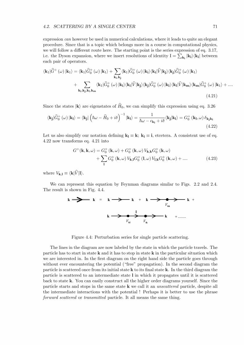
4.2. SCATTERING BY A SINGLE CENTER 71
expression can however be used in numerical calculations, where it leads to quite an elegantprocedure. Since that is a topic which belongs more in a course in computational physics,we will follow a different route here. The starting point is the series expression of eq. 3.17,i.e. the Dyson expansion, where we insert resolutions of identity I =
Pki|kiihki| between
each pair of operators.
hk1| bG+ (ω) |k1i = hk1| bG+0 (ω) |k1i+Xki,kj
hk1| bG+0 (ω) |kiihki|bV |kjihkj| bG+0 (ω) |k1i+
Xki,kj,kl,km
hk1| bG+0 (ω) |kiihki|bV |kjihkj| bG+0 (ω) |klihkl|bV |kmihkm| bG+0 (ω) |k1i+ ....(4.21)
Since the states |ki are eigenstates of bH0, we can simplify this expression using eq. 3.26hkj| bG+0 (ω) |kli = hkj|³~ω − bH0 + iδ´−1 |kli = 1
~ω − ²kl + iδhkj|kli = G+0 (kl,ω) δkjkl
(4.22)
Let us also simplify our notation defining kl ≡ k; ki ≡ i, etcetera. A consistent use of eq.4.22 now transforms eq. 4.21 into
G+(k,k,ω) = G+0 (k,ω) +G+0 (k,ω)Vk,kG
+0 (k,ω)
+Xl
G+0 (k,ω)Vk,lG+0 (l,ω)Vl,kG
+0 (k,ω) + .... (4.23)
where Vk,l ≡ hk|bV |li.We can represent this equation by Feynman diagrams similar to Figs. 2.2 and 2.4.
The result is shown in Fig. 4.4.
kk = kk +kkV
k k +
klV lkVk k
l........+
Figure 4.4: Perturbation series for single particle scattering.
The lines in the diagram are now labeled by the state in which the particle travels. Theparticle has to start in state k and it has to stop in state k in the particular situation whichwe are interested in. In the first diagram on the right hand side the particle goes throughwithout ever encountering the potential (“free” propagation). In the second diagram theparticle is scattered once from its initial state k to its final state k. In the third diagram theparticle is scattered to an intermediate state l in which it propagates until it is scatteredback to state k. You can easily construct all the higher order diagrams yourself. Since theparticle starts and stops in the same state k we call it an unscattered particle, despite allthe intermediate interactions with the potential ! Perhaps it is better to use the phraseforward scattered or transmitted particle. It all means the same thing.
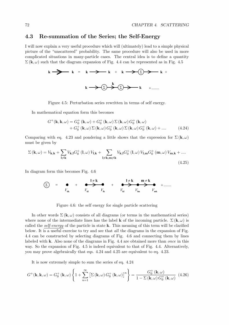
72 CHAPTER 4. SCATTERING
4.3 Re-summation of the Series; the Self-Energy
I will now explain a very useful procedure which will (ultimately) lead to a simple physicalpicture of the “unscattered” probability. The same procedure will also be used in morecomplicated situations in many-particle cases. The central idea is to define a quantityΣ (k,ω) such that the diagram expansion of Fig. 4.4 can be represented as in Fig. 4.5
kk = kk + k k +
k k ........+
Σ
Σ Σk
Figure 4.5: Perturbation series rewritten in terms of self energy.
In mathematical equation form this becomes
G+(k,k,ω) = G+0 (k,ω) +G+0 (k,ω)Σ (k,ω)G
+0 (k,ω)
+G+0 (k,ω)Σ (k,ω)G+0 (k,ω)Σ (k,ω)G
+0 (k,ω) + .... (4.24)
Comparing with eq. 4.23 and pondering a little shows that the expression for Σ (k,ω)must be given by
Σ (k,ω) = Vk,k +Xl6=k
Vk,lG+0 (l,ω)Vl,k +
Xl6=k,m6=k
Vk,lG+0 (l,ω)Vl,mG
+0 (m,ω)Vm,k + ....
(4.25)
In diagram form this becomes Fig. 4.6
Σ =
kkV+
klV lkV
kl ≠+
lmV
kl ≠ km ≠
klV mkV........+
Figure 4.6: the self energy for single particle scattering
In other words Σ (k,ω) consists of all diagrams (or terms in the mathematical series)where none of the intermediate lines has the label k of the incoming particle. Σ (k,ω) iscalled the self-energy of the particle in state k. This meaning of this term will be clarifiedbelow. It is a useful exercise to try and see that all the diagrams in the expansion of Fig.4.4 can be constructed by selecting diagrams of Fig. 4.6 and connecting them by lineslabeled with k. Also none of the diagrams in Fig. 4.4 are obtained more than once in thisway. So the expansion of Fig. 4.5 is indeed equivalent to that of Fig. 4.4. Alternatively,you may prove algebraically that eqs. 4.24 and 4.25 are equivalent to eq. 4.23.
It is now extremely simple to sum the series of eq. 4.24
G+(k,k,ω) = G+0 (k,ω)
(1 +
∞Xn=1
£Σ (k,ω)G+0 (k,ω)
¤n)=
G+0 (k,ω)
1− Σ (k,ω)G+0 (k,ω)(4.26)
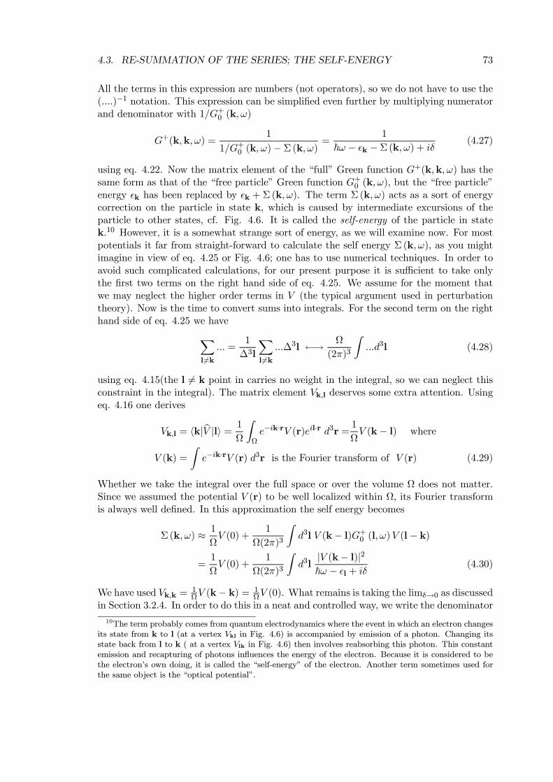
4.3. RE-SUMMATION OF THE SERIES; THE SELF-ENERGY 73
All the terms in this expression are numbers (not operators), so we do not have to use the(....)−1 notation. This expression can be simplified even further by multiplying numeratorand denominator with 1/G+0 (k,ω)
G+(k,k,ω) =1
1/G+0 (k,ω)− Σ (k,ω)=
1
~ω − ²k − Σ (k,ω) + iδ (4.27)
using eq. 4.22. Now the matrix element of the “full” Green function G+(k,k,ω) has thesame form as that of the “free particle” Green function G+0 (k,ω), but the “free particle”energy ²k has been replaced by ²k + Σ (k,ω). The term Σ (k,ω) acts as a sort of energycorrection on the particle in state k, which is caused by intermediate excursions of theparticle to other states, cf. Fig. 4.6. It is called the self-energy of the particle in statek.10 However, it is a somewhat strange sort of energy, as we will examine now. For mostpotentials it far from straight-forward to calculate the self energy Σ (k,ω), as you mightimagine in view of eq. 4.25 or Fig. 4.6; one has to use numerical techniques. In order toavoid such complicated calculations, for our present purpose it is sufficient to take onlythe first two terms on the right hand side of eq. 4.25. We assume for the moment thatwe may neglect the higher order terms in V (the typical argument used in perturbationtheory). Now is the time to convert sums into integrals. For the second term on the righthand side of eq. 4.25 we haveX
l 6=k... =
1
∆3l
Xl6=k
...∆3l ←→ Ω
(2π)3
Z...d3l (4.28)
using eq. 4.15(the l 6= k point in carries no weight in the integral, so we can neglect thisconstraint in the integral). The matrix element Vk,l deserves some extra attention. Usingeq. 4.16 one derives
Vk,l = hk|bV |li = 1
Ω
ZΩe−ik·rV (r)eil·r d3r =
1
ΩV (k− l) where
V (k) =
Ze−ik·rV (r) d3r is the Fourier transform of V (r) (4.29)
Whether we take the integral over the full space or over the volume Ω does not matter.Since we assumed the potential V (r) to be well localized within Ω, its Fourier transformis always well defined. In this approximation the self energy becomes
Σ (k,ω) ≈ 1
ΩV (0) +
1
Ω(2π)3
Zd3l V (k− l)G+0 (l,ω)V (l− k)
=1
ΩV (0) +
1
Ω(2π)3
Zd3l
|V (k− l)|2~ω − ²l + iδ (4.30)
We have used Vk,k =1ΩV (k− k) = 1
ΩV (0). What remains is taking the limδ→0 as discussedin Section 3.2.4. In order to do this in a neat and controlled way, we write the denominator
10The term probably comes from quantum electrodynamics where the event in which an electron changesits state from k to l (at a vertex Vkl in Fig. 4.6) is accompanied by emission of a photon. Changing itsstate back from l to k ( at a vertex Vlk in Fig. 4.6) then involves reabsorbing this photon. This constantemission and recapturing of photons influences the energy of the electron. Because it is considered to bethe electron’s own doing, it is called the “self-energy” of the electron. Another term sometimes used forthe same object is the “optical potential”.
74 CHAPTER 4. SCATTERING
of the integrand as
1
~ω − ²l + iδ =(~ω − ²l)
(~ω − ²l)2 + δ2− iδ
(~ω − ²l)2 + δ2(4.31)
The first term on the right hand side of this expression contributes to the real part of theself energy Σ (k,ω) and the second term contributes to its imaginary part. The real partgives the so-called “principal value” or Pv of the integral.11
ReΣ (k,ω) =1
Ω
½V (0) +
1
(2π)3Pv
Zd3l
|V (k− l)|2~ω − ²l
¾(4.32)
More about Pv ’s can be found in the appendix on complex analysis. Also there you canfind there the proof of
limη→0+
1
π
η
x2 + η2= δ(x) (4.33)
i.e. a Lorentzian line-shape function in the limit of vanishing width becomes a δ-function.Using this property for the second term on the right hand side of eq. 4.31 then gives forthe imaginary part of the self-energy
ImΣ (k,ω) = −π 1
Ω(2π)3
Zd3l |V (k− l)|2δ(~ω − ²l) (4.34)
The integrals in eqs. 4.32 and 4.34 can usually be done, and thus one finds a closedexpression for the self energy Σ (k,ω). We see now why it is a peculiar object. It hasthe dimension of energy and it depends upon the state k and upon the frequency ω. Thestrange thing is that it has an imaginary part as well as a real part. This might seemweird for an “energy”, but it has clear physical consequences, which are discussed in thenext subsection.
4.4 The Physical Meaning of Self-Energy
Let us go back to our starting point. Starting with the particle in state k at time t1, theprobability amplitude that the particle is still in state k at time t2 is given by
hk|bU (t2 − t1) |ki = i~2π
Z ∞
−∞dω
e−iω(t2−t1)
~ω − ²k −Σ (k,ω) (4.35)
according to eqs. 4.20 and 4.27. The integral can be done by complex contour integration(a short summary of complex function analysis is given in the appendix).12 What is neededare the “poles” of the integrand, i.e. the roots of the denominator, or the solutions ω ofthe equation
~ω − ²k − Σ (k,ω) = 0 (4.36)
11The principal value of the integral is calculated by using the first term on the right handside of eq.4.31 in the integral. Then one does the integration, and finally one takes limδ→012We have taken limδ→0 already. This is o.k. here; since ImΣ (k,ω) < 0 the integral can be done without
needing the δ-trick.
4.4. THE PHYSICAL MEANING OF SELF-ENERGY 75
Read the appendix if this does not make any sense to you. Because of the ω dependenceof Σ (k,ω) this is a nontrivial equation to solve, but we could solve it iteratively, usingknowledge of our approximated Σ (k,ω), cf. eqs. 4.32 and 4.34. Because we have usedonly the first few terms of a perturbation series to derive those equations, we have alreadyassumed that the perturbation V is small. But this then must mean that Σ (k,ω) cannot betoo large. We can start solving eq. 4.36 by setting Σ (k,ω) = 0 in zeroth order, which gives~ω(0) = ²k. In the next iteration we then solve the equation ~ω(1) − ²k − Σ
¡k,ω(0)
¢= 0,
which gives ~ω(1) = ²k+Σ (k, ²k/~). Note that ω(1) is a complex number, since Σ (k, ²k/~)is complex. In principle we can pursue these iterations solving ~ω(n)−²k−Σ
¡k,ω(n−1)
¢=
0; n = 2, 3... which converges to some point ω(∞). In numerical analysis one calls thismathematical algorithm “fixed point iteration”, since one converges onto a “fixed” point.Having found the pole, the next step is to find the “residue”. The details of the derivationare a bit messy, but they are explained at great length in the appendix, Subsection 4.8.4.We assume that |ImΣ (k,ω)| is small, so we can use eq. 4.97. The result isZ ∞
−∞dω
e−iω(t2−t1)
~ω − ²k − Σ (k,ω) =2π
i~zke
− i~ [²k+∆k− i~
2Γk](t2−t1) for t2 > t1
= 0 for t2 < t1 (4.37)
where the second line follows from the fact that ImΣ (k,ω) < 0 (eq. 4.34 and the ap-pendix). The factors in this equation are given by (see eq. 4.97)
zk =
µ1− 1
~∂ReΣ (k,ω)
∂ω|ω=²k/~
¶−1= 1
∆k = ReΣ (k, ²k/~)
Γk = −2zk~ImΣ (k, ²k/~) (4.38)
Using these results in eq. 4.35 we finally get the answer we were looking for
hk|bU (t2 − t1) |ki = zke− i~ [²k+∆k](t2−t1)e−
12Γk(t2−t1) for t2 > t1 (4.39)
Comparing this with the time evolution of a free particle without scattering potentialpresent
hk|bU0 (t2 − t1) |ki = e− i~ ²k(t2−t1)
we see that three remarkable things happened by the introduction of the scattering po-tential V
1. The energy level of the particle has shifted from ²k to ²k +∆k. Note that theenergy shift ∆k within our approximation is exactly what you would have foundby applying up to 2nd order time-independent perturbation theory on the state |ki.This is most clearly seen be rewriting this equation in the discrete sum representationagain (using eqs. 4.28 and 4.29).
∆k = ReΣ (k, ²k/~) = Vkk +Xl 6=k
|Vkl|2²k − ²l (4.40)
76 CHAPTER 4. SCATTERING
2. The probability amplitude is decaying exponentially by a characteristic lifetime given
by τk =1Γk. The probability that a particle stays in state k is given by
Wk→k = |hk|bU (t2 − t1) |ki|2 ∝ e−Γk(t2−t1)Thus the characteristic decay time of the exponential decay is given by τk = Γ
−1k .
If the decay time is long, the particle still resembles very much a free particle andthe standard term for such a particle is quasi-particle. The decay rate Γk containsa factor Ω−1, cf. eqs. 4.32 and 4.34. Referring to our introduction in Section 4.1,we observe that
Ω−1 = nI
the concentration of gas atoms. It makes clean physical sense that the decay rateis proportional to the concentration of scattering centers the incoming particle en-counters.
3. The probability amplitude is multiplied by a factor zk. In this particular case we can
easily show that zk = 1. This is because hk|bU (t1 − t1) |ki = hk|I||ki = 1, accordingto eq. 4.17 and eq. 2.7 in Chapter 2. So here we have
∂ReΣ (k, ²k/~)∂ω
= 0 (4.41)
This is true for a single particle, but is no longer true in the many particle case.Anticipating later chapters, one can prove that in the general many particle case onestill finds the quasi-particle form of eq. 4.39, but now 0 < zk ≤ 1. So zk acts as aweight factor for the quasi-particle probability amplitude. In the single particle casethis weight factor is always one.
Connection with Fermi’s Golden Rule
Now have a look back at Fermi’s golden rule, eq. 2.32. The perturbation V is frequencyindependent in the scattering considered here, so we can set ω = 0 in eq. 2.32; moreoverωlk =
²k−²l~ and we can use the relation δ(ax) = 1
aδ(x). So from Fermi’s golden rule wededuce that the transition rate from state k to a different state l is
wk→l =2π
~|Vk,l|2δ(²k − ²l) = 2π
~Ω2|V (k− l)|2δ(²k − ²l) (4.42)
using eq. 4.29. From eqs. 4.34 and 4.38 we now have established
Γk =Ω
(2π)3
Zd3l wk→l =
Xl6=k
wk→l (4.43)
when returning to the discrete sum representation again (eq. 4.28 ) This expresses the factthat the decay rate of the probability of staying in state k is equal the sum of transitionrates to all other states l. Thus the sum of the probabilities of the particle being in statek or in one of the other states l is one. So eq. 4.43 is the quantum mechanical expressionof “conservation of particles”. Conservation of particles must of course always be valid.So even if one has to include higher order perturbation terms to calculate the transitionrates wk→l (and not just the first order term that lead to Fermi’s golden rule), then stilleq. 4.43 is valid.
4.5. THE SCATTERING CROSS SECTION 77
4.5 The Scattering Cross Section
Setting up a scattering experiment, one usually does work with only a single particle.Instead, one tries to prepare a stable beam of incoming particles, all with the same mo-
mentum p = ~k and energy ²k = (~k)22m , i.e. a “monochromatic” beam. Experimentally,
it is the particle flux Φin of the beam one aims to stabilize at a constant value. Theflux is defined as Φin = Nv, where N is the density of particles in the beam and v=~k
mis their speed. The total number of scattered particles per second is equal to the sumof the transition rates to all possible states, which according to eq. 4.43 is equal to Γk.According to its definition in Section 4.1.1, the total cross section is therefore given by
σk = Γk/Φin (4.44)
Often one omits the subscript k on σk since the dependence is clear from the context.In the calculations of the previous three sections we have assumed a density of incomingparticles of N = Ω−1, since we have chosen to normalize our incoming plane wave suchthat we have one particle per box of volume Ω, see eq. 4.16. Therefore in our case theflux is Φin =
vΩ . Using eq. 4.38, and realizing that Ω
−1 = nI , since we also have only onescattering center per box. The scattering cross section σ = Γk/Φin then becomes
σ = −2 ImΣ (k, ²k/~)nI~v
(4.45)
Comparing this to eq. 4.13 in Section 4.1.1 we must have13
fkk = − m
2π~2nIΣ (k, ²k/~) (4.46)
Eq. 4.45 is thus merely a restatement of the optical theorem.14; fkk is called the forwardscattering amplitude and we have found a way to calculate it (and the cross section). Inthe simple perturbation approximation which gave rise to eqs.4.30 and 4.34 we get theexpression
Im fkk = − m
2π~21
(2π)3
Zd3l |V (k− l)|2δ(²k − ²l) (4.47)
which is simply restating eq. 4.43 again. Comparing eqs. 4.47 and 4.14, one gets thefeeling that the right hand side of eq. 4.47 must incorporate an approximation to thescattering amplitudes flk. We will have a look at these in the next sections.
4.5.1 The Lippmann-Schwinger Equation
No doubt the reader will have noticed a difference in point of view between sections 4.2and 4.1. In section 4.2 we introduced a single particle at a specific time t1 and followedits time evolution up to time t2. In section 4.1 we considered a beam of particles in asteady state situation, i.e. the number of incoming and scattered particles per unit timeis constant. The scattered wave form of eq. 4.1 describes such a steady state situation.Obviously the times of creation and detection of individual particles do not play a role
13Formally, we have only proved it for the imaginary part, but it holds for the real part as well.14Which is probably why the self-energy is also called the optical potential.
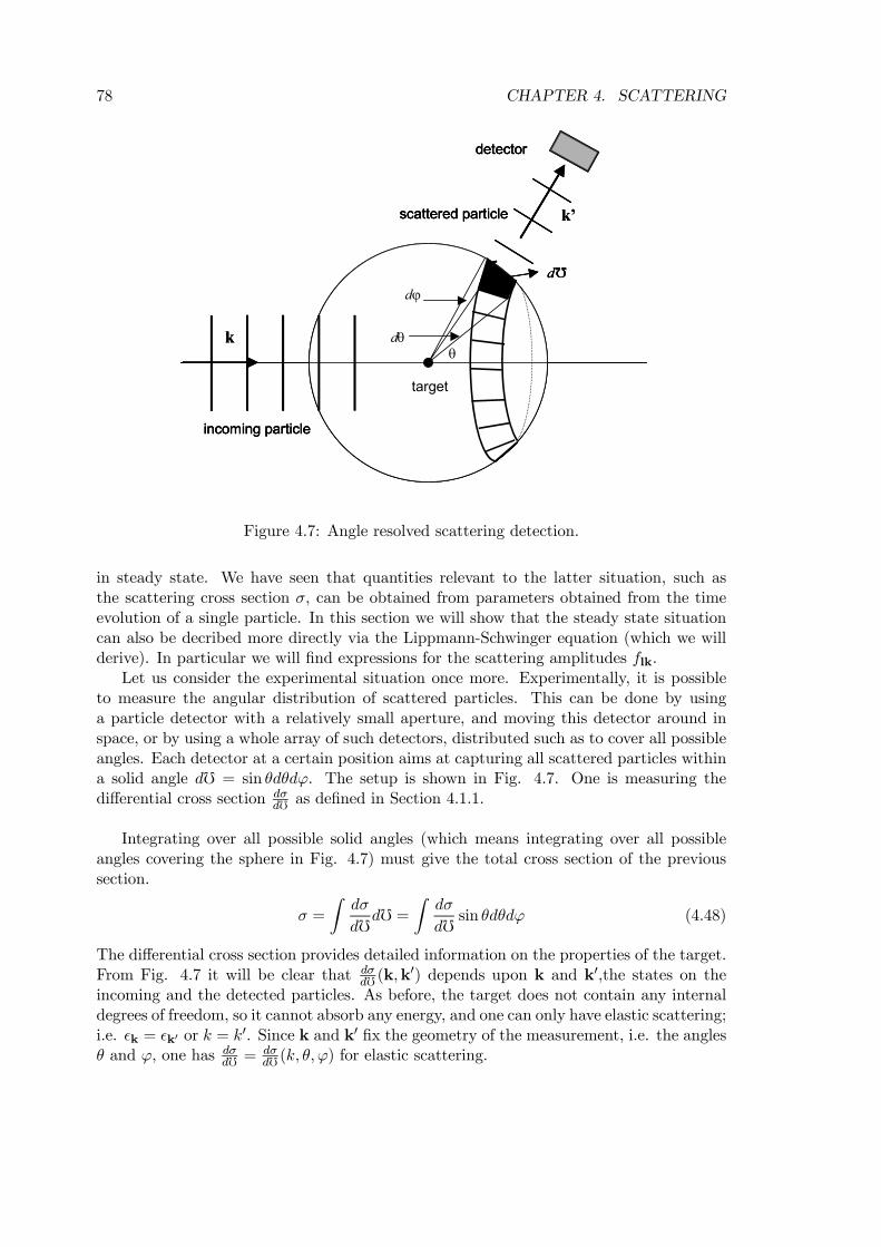
78 CHAPTER 4. SCATTERING
θdθ
dϕd
target
scattered particle
incoming particle
detector
k
k’
θdθ
dϕd
target
scattered particle
incoming particle
detector
θdθ
dϕd
target
scattered particle
incoming particle
detector
k
k’
Figure 4.7: Angle resolved scattering detection.
in steady state. We have seen that quantities relevant to the latter situation, such asthe scattering cross section σ, can be obtained from parameters obtained from the timeevolution of a single particle. In this section we will show that the steady state situationcan also be decribed more directly via the Lippmann-Schwinger equation (which we willderive). In particular we will find expressions for the scattering amplitudes flk.
Let us consider the experimental situation once more. Experimentally, it is possibleto measure the angular distribution of scattered particles. This can be done by usinga particle detector with a relatively small aperture, and moving this detector around inspace, or by using a whole array of such detectors, distributed such as to cover all possibleangles. Each detector at a certain position aims at capturing all scattered particles withina solid angle df = sin θdθdϕ. The setup is shown in Fig. 4.7. One is measuring thedifferential cross section dσ
df as defined in Section 4.1.1.
Integrating over all possible solid angles (which means integrating over all possibleangles covering the sphere in Fig. 4.7) must give the total cross section of the previoussection.
σ =
Zdσ
dfdf =
Zdσ
dfsin θdθdϕ (4.48)
The differential cross section provides detailed information on the properties of the target.From Fig. 4.7 it will be clear that dσ
df (k,k0) depends upon k and k0,the states on the
incoming and the detected particles. As before, the target does not contain any internaldegrees of freedom, so it cannot absorb any energy, and one can only have elastic scattering;i.e. ²k = ²k0 or k = k
0. Since k and k0 fix the geometry of the measurement, i.e. the anglesθ and ϕ, one has dσ
df =dσdf (k, θ,ϕ) for elastic scattering.
4.5. THE SCATTERING CROSS SECTION 79
The rest of this section aims at (1) finding an equation which describes the steadystate situation more directly and then (1) obtaining a quantum mechanical expression forthe differential scattering cross section. Let us start as in Section 4.2 by looking at thetime evolution of a single particle in an incoming state |ki, or its Fourier transform, cf.eq. 4.20
bU(t2 − t1)|ki FTÀ bG+ (ω) |ki ; t2 > t1 (4.49)
We then can use the Dyson equation of eq. 3.21 and write the right hand side of eq. 4.49as
bG+ (ω) |ki = bG+0 (ω) |ki+ bG+0 (ω) bV bG+ (ω) |ki (4.50)
We recognize that by Fourier transforming bG+ (ω) |ki we get the complete time evolutionof the incoming particle. Obviously from bG+0 (ω) |ki one then gets the time evolution ofthe unperturbed system, in absence of the scattering potential bV . We know that
bG+0 (ω) |ki = |ki~ω − ²k + iη (4.51)
The factor (~ω−²k+iη)−1 is handled the following way. We Fourier transform to the timedomain according to eq. 4.20. The Fourier transform can be calculated using complexcontour integration (see the Appendix, Section 4.8.2). One gets
|ψk,0(t)i =i~2π
Z ∞
−∞dω e−iωt bG+0 (ω) |ki = |kie− i
~ (²k−iη)t ; t > 0 (4.52)
= 0 ; t ≤ 0
see eq. 4.85 in Appendix II. Remember that η is a very small positive number, which leadsto a factor exp(−ηt/~). This damps the state, but as long as ~/η À any measuring time,this factor has no physically observable effect, and is only a mathematically convenienttrick. Eq. 4.52 describes the time evolution of an unperturbed particle which is createdat t = 0 (and does not exist before that time) in state |ki. Sudden creation of a particleobviously does not describe a steady state. But now have a look at the following state
|φk,0(t)i = |kie− i~ (²k−iη)t ; t > 0 (4.53)
= |kie− i~ (²k+iη)t ; t ≤ 0
The bottom line involves a factor exp(+ηt/~), which goes to zero for t → −∞. Thisexpression describes a state which is very slowly switched on from t = −∞ to t = 0 anddies out (very slowly) again to t =∞. It is called an adiabatically switched-on (and -off)state, in contrast to Eq. 4.52, which is called a suddenly switched-on state. Adiabaticallyswitching-on allows for a gentle approach to a steady state situation. Letting limη→0 gives
limη→0 |φk,0(t)i = |kie
− i~ ²kt (4.54)
which is the familiar expression known from elementary quantum mechanics. Eq. 4.53 isvery similar to this, but it describes a state with well-defined limits at t = ∓∞. We expect
80 CHAPTER 4. SCATTERING
this to be a state of a well-defined energy ²k from the similarity with Eq. 4.54. This canbe verified explicitly by Fourier transformation
|φk,0(ω)i =1
i~
Z ∞
−∞dt eiωt|φk,0(t)i
=|ki
~ω − ²k + iη −|ki
~ω − ²k − iη=
2π
i~|kiδ(ω − ²k/~) (4.55)
where we have used Eq. 4.93 in Appendix II. Now we are almost there. An expression forthe suddenly switched-on state can be found by rewriting the Dyson equation, Eq. 4.50,as
|ψk(ω)i = bG+ (ω) |ki = ³I− bG+0 (ω) bV ´−1 bG+0 (ω) |ki (4.56)
=³I− bG+0 (ω) bV ´−1 |ψk,0(ω)i
Since the Dyson equation is only the Schrodinger equation in disguise, the same must holdfor an adiabatically switched-on state
|φk(ω)i =³I− bG+0 (ω) bV ´−1 |φk,0(ω)i
=2π
i~
³I− bG+0 (²k/~) bV ´−1 |kiδ(ω − ²k/~) (4.57)
≡ 2π
i~|φkiδ(ω − ²k/~) (4.58)
where we recognize that bG+0 can only give a contribution if ω = ²k/~, since f(x)δ(x−a) =f(a)δ(x−a). The bottom line is a definition of the state |φki. To get the time dependenceone can Fourier transform according to the prescription
|φk(t)i =i~2π
Z ∞
−∞dω e−iωt|φk(ω)i
=
Z ∞
−∞dω e−iωtδ(ω − ²k/~)|φki = |φkie−
i~ ²kt (4.59)
It descibes a state with at an energy ²k, in which the effect of the scattering potentialis fully taken into account. Comparing Eqs. 4.57 and 4.58 and deleting the δ(ω − ²k/~)factors we get
|φki =³I− bG+0 (²k/~) bV ´−1 |ki
which is equivalent to
|φki = |ki+ bG+0 (²k/~) bV |φki (4.60)
This equation is called the Lippmann-Schwinger equation.. As we can see, the ω-dependenceis not really necessary. We can work with |φki and |ki, which are related by eq. 4.60; theirtime dependence is obtained by multiplying with e−
i~ ²kt, cf. eqs. 4.54 and 4.59. From
the Lippmann-Schwinger equation on can calculate the scattering state |φki from the un-perturbed state |ki, where both have the fixed energy ²k . Remember that quantum me-chanically fixed energy means fized frequency and it is clear that the Lippmann-Schwingerequation describes the situation of section 4.1.
4.5. THE SCATTERING CROSS SECTION 81
Connection to the time-independent Schrodinger equation
The Lippmann-Schwinger equation, Eq. 4.60, describes the scattering of particles at afixed energy ²k =
~2k22m , which is the energy of the incoming particle. It is easy to show
that |φki is the eigenstate of the full Hamiltonian with eigenvalue ²k. From eq. 4.60 onegets
(²k − bH0)|φki = (²k − bH0)|ki+ (²k − bH0) bG+0 (²k/~) bV |φki= (²k − ²k)|ki+ IbV |φki⇔
( bH0 + bV )|φki = ²k|φki (4.61)
where we have used eq. 3.28 of Section 3.2.4. The bottom line is the time-independentSchrodinger equation, familar from elementary quantum mechanics. Following the stepsfrom eq. 4.61 to eq. 4.60 backwards is another way to derive the Lippmann-Schwingerequation. It shows that the latter is completely equivalent to the time-independentSchrodinger equation.15 In conclusion, the main difference between sections 4.2 and 4.1is the use of a time-dependent Schrodinger picture in the former, and a time-independentone in the latter.
Wave functions
We are interested in the spatial behavior of the Lippmann-Schwinger equation, i.e. in theposition representation or the wave function φk(r) = hr|φki and we will show that it willgive the wave form of eq. 4.1 in Section 4.1. Inserting a couple of resolutions of identityin eq. 4.60 one obtains
φk(r) = hr|φki = hr|ki+ hr| bG+0 (²k/~) bV |φki= hr|ki+
Z Zd3r0d3r00 hr| bG+0 (²k/~)|r0ihr0|bV |r00ihr00|φki
=1√Ωeik·r +
Zd3r0 hr| bG+0 (²k/~) |r0iV (r0)φk(r0) (4.62)
where we have used eqs. 4.16; the last line follows from hr0|bV |r00i = V (r00)hr0|r00i =V (r00)δ(r0 − r00). The interesting bit is
hr| bG+0 (²k/~) |r0i =Xk00,k0
hr|k00ihk00| bG+0 (²k/~) |k0ihk0|r0i=
Xk00,k0
hr|k00ihk0|r0i²k − ²k0 + iδ δk,k
0
=1
(2π)3
Zd3k0
eik0·(r−r0)
²k − ²k0 + iδ (4.63)
15The nomenclature is slightly confusing. Both the forms of eq. 4.60 and 3.59 in the appendix of theprevious chapter, are called the Lippman-Schwinger equation. Eq. 3.59 works in the time domain and isequivalent to the time-dependent Schrodinger equation. Eq. 4.60 works at a fixed energy and is equivalentto the time-independent Schrodinger equation. If you want a delicate mathematical proof that both formsgive equivalent results, see R. G. Newton, Scattering Theory of Waves and Particles, (Springer, New York,1982); Ch. 6,7.
82 CHAPTER 4. SCATTERING
where we have used eqs. 4.16, 4.22 and 4.28. Note that we could have immediatelyobtained this result from eqs. 3.30 and 3.31. Knowing that ²k0 =
~2k022m , the integral of eq.
4.63 can be done.16 The end result is quite simple and elegant
hr| bG+0 (²k/~) |r0i = − m
2π~2eik|r−r0|
|r− r0| (4.64)
So eq. 4.62 becomes
φk(r) =1√Ωeik·r − m
2π~2
Zd3r0
eik|r−r0|
|r− r0| V (r0)φk(r
0) (4.65)
This is the real space representation of the Lippmann-Schwinger equation.
4.5.2 The Scattering Amplitudes and the Differential Cross Section
The first term on the right hand side of eq. 4.65 is the plane wave which describes theincoming particle; the second term on the right hand side describes the scattered wave.The potential V (r0) which describes the target has a finite range and it decays fast outsidethe target. So whereas the integral
Rd3r0 in principle goes over Ω (the volume of the box
we used to normalize our states), in practice V (r0) ensures that one only has to integrateover a small volume which contains the target. The position r at which the scatteredparticles are detected is far from the target. The target is a microscopic particle, sor0 . 10−14− 10−9m, whereas the detector is part of a macroscopic laboratory experiment,so typically r ∼ 10−2 − 101m. In other words, we are interested in the limit r À r0 in eq.4.65. In this limit we can make the approximation¯
r− r0¯ ≈ r − er · r0where er is a unit vector in the direction of the detector r and therefore
eik|r−r0|
|r− r0| ≈eikr
re−iker·r
0
Defining k0 = ker, a wave vector in the direction of the detector with the same size asthat of the incoming wave, we get
φk(r) −→r large
1√Ωeik·r − m
2π~2eikr
r
Zd3r0 e−ik
0·r0V (r0)φk(r0)
=1√Ωeik·r − m
√Ω
2π~2eikr
r
Zd3r0 hk0|r0iV (r0)hr0|φki
=1√Ωeik·r − m
√Ω
2π~2eikr
rhk0|bV |φki (4.66)
Defining a quantity fk0k by
fk0k =mΩ
2π~2hk0|bV |φki (4.67)
16If you want to try and do it yourself. Write d3k0 = k02dk0d(cos θ)dϕ in spherical coordinates and
eik·(r−r0) = eik|r−r
0| cos θ, where θ is defined as the angle between k0 and (r− r0). First do the integral overdϕ and then the integral over d(cos θ). The remaining integral over dk0 can be done by contour integration,as discussed in the Appendix.
4.5. THE SCATTERING CROSS SECTION 83
we obtain
φk(r) −→r large
1√Ω
·eik·r − e
ikr
rfk0k
¸(4.68)
Adding the time factor e−i~ ²kt as in eq. 4.59, we see that this corresponds to the wave form
of eq. 4.1 in Section 4.1 (which actually proves that this wave form that was postulatedon “intuitive” grounds, is correct). Eq. 4.67.now gives a way to calculate the scatteringamplitudes fk0k.
Just one more step brings us to the differential cross section. Imagine that the largesphere in Fig. 4.7 has a radius r, then the flux Φ(θ,ϕ) of scattered particles through theblack surface element of that sphere is
Φ(θ,ϕ) = probability density at surface × area surface element × speed particle=
|fk0k|2Ωr2
× r2df× v (4.69)
One has to divide this by the incoming flux Φin =vΩ (see the previous section) and the
solid angle df to get the differential cross section according to its definition
dσ
df=Φ(θ,ϕ)
Φindf= |fk0k|2 (4.70)
Comparing eq. 4.66 to eq. 4.68 one finds the final elegant result
dσ
df= |fk0k|2 = m2Ω2
4π2~4|hk0|bV |φki|2 (4.71)
4.5.3 The Born Series and the Born approximation
The occurrence of |φki in this expression supposes that one knows the solution of theLippmann-Schwinger equation, eq. 4.60. If one does not, one can get successive betterapproximations by applying a series expansion of eq. 4.60 in the same spirit as the Dysonexpansion, cf. eq. 3.17
|φki = |ki+ bG+0 (²k/~) bV |ki+ bG+0 (²k/~) bV bG+0 (²k/~) bV |ki+ ..... (4.72)
Although it is actually the same thing as the Dyson expansion, in scattering theory thisis called the Born series. If one neglects all terms beyond the first one on the right handside of eq. 4.72, one defines the so-called “Born approximation” for eq. 4.71
dσ1df
=m2Ω2
4π2~4|hk0|bV |ki|2 = m2
4π2~4|V (k0 − k)|2 (4.73)
according to eq. 4.29. In the context of scattering theory “the Born approximation” hasthis very specific meaning. We can prove that it is equivalent to what can be obtained by
84 CHAPTER 4. SCATTERING
Fermi’s golden rule. The total cross section in this approximation is given by
σ1 =
Zdσ1df
sin θdθdϕ =1
k2
Zdσ1df
k2 sin θdθdϕ
=m2
4π2~4k2
Z|V (k− k0)|2δ(k − k0)k02 sin θdθdϕ
=m2
4π2~4k2~2km
Z|V (k− k0)|2δ(²k − ²k0)d3k0
=1
4π2~v
Z|V (k− k0)|2δ(²k − ²k0)d3k0 (4.74)
using δ(b(x2−a2)) = 12abδ(x−a) and v = ~k
m . This corresponds to eqs. 4.45 and 4.47. Wehave now found three separate ways to find the total cross section in this approximation.
1. Using eq. 4.44, which needs the decay rate Γk. This is related to the self-energy Σ,via eq. 4.38. The self-energy is then approximated via eq. 4.30.
2. Again using eq. 4.44, but now obtaining the decay rate Γk using the “conservationof particles” and Fermi’s golden rule, cf. eqs. 4.42 and 4.43.
3. Using the differential cross section in the “Born approximation”, eq. 4.73, andintegrating over all angles.
The equivalence of 2. and 3. shows that the physical content of Fermi’s golden ruleand the “Born approximation” is essentially the same. This should not be surprising,since if we follow the derivation of the differential cross section backwards, from eq. 4.74to eq. 4.60, one observes that the “Born approximation” of eq. 4.73 can be obtained byreplacing |φki by |ki at the right hand side of eq. 4.60. So we make the approximation
|φki ≈ |ki+ bG+0 (²k/~) bV |ki (4.75)
Going back from eq. 4.60 to eq. 4.50, one observes that this corresponds to the approxi-mation for the Green function operatorbG+ (ω) ≈ bG+0 (ω) + bG+0 (ω) bV bG+0 (ω) (4.76)
But this is essentially nothing else than the Fourier transform of the expression we got infirst order perturbation theory, cf. eq. 2.23 in Section 2.3, from which we derived Fermi’sgolden rule. “First order perturbation theory” was called the “Born approximation” inthat section; now we see that it is consistent with the use of this phrase in scatteringtheory.
The Born approximation is used a lot in scattering theory, because it is so simple. Tocalculate the differential cross section one only needs the Fourier transform of the scatteringpotential, cf. eqs. 4.73 and 4.29. Unfortunately it does not always give accurate results;if the scattering potential bV is large, neglect of the higher order perturbation terms is notallowed. For moderately strong potentials, one can add subsequent higher order termsas in eq. 4.72. Nowadays, for single particle scattering it is also possible to solve theLippmann-Schwinger equation (eq. 4.60) numerically on a fast computer, usually usingthe real space representation of eq. 4.65. From the numerical function |φki one thencalculates the differential cross section of eq. 4.71, and by numerical integration over allangles the total cross section. The procedure can be quite involved, since one is usuallyinterested in knowing the latter for a whole range of k-values.
4.6. EPILOGUE 85
4.6 Epilogue
A final word about this chapter. It might seem that we made it lot of fuss about thingsthat could have been derived simply from Fermi’s golden rule, eq. 2.32. We can obtainthe transition rates wk→l, eq. 4.42 from Fermi’s golden rule. From the “conservation ofparticles” we can establish that this leads to an exponentially decaying probability of theparticle staying in state k, with a rate Γk given by eq. 4.43. This short-cut would havesaved us an enormous amount of equation deriving.17 However I did not take the detourfor you just to admire the scenery; it has given us some important road signs for the future(quasi-particles and self energies). The quasi-particle result, eq. 4.39, is much more generalthan what could be obtained under Fermi’s rule. We can make better approximations tothe self energy Σ (k,ω) than just the first two terms of the perturbation expansion as ineq. 4.30. The “pole” equation 4.36 can also be solved to any accuracy to obtain a rootωk. It may require extra work and even some numerical computing to obtain accurateresults, but the general equation, eq. 4.39, still stands.
Also it might seem strange that we speak of a quasi-particle when obviously we havebeen dealing with a well-defined single particle all the time. This term however remainsuseful in a more complicated environment. Imagine that we have a large number scatteringcenters that are not very far apart, like in a dense gas, or a dirty metal full of impurities.The particle (e.g. an electron) is then a pinball in a giant (1017—1023 atoms) pinball ma-chine. Multiple scattering from many centers leads to a complicated interference patternof scattered waves and to very complicated particle states. Yet one can prove that thegeneral equation 4.39 is still valid. Even if one takes into account all the electrons in thecrystal when adding an extra one - we then have a giant number (1023) of pinballs in agiant pinball machine - even then eq. 4.39 is still relevant for describing the time evolutionor propagation of the extra electron. Of course one looses track of the individual particlesamidst all this scattering. As we will see later on, quantum mechanics tells us that elec-trons are indistinguishable, so it is even fundamentally impossible to track a single electronin the pinball machine. Yet, as long as we have a time dependence which is given by eq.4.39, we quasi still have a single particle, or in other words a quasi-particle. Whether thequasi-particle concept is useful in practical situations depends on the numerical value ofthe lifetime τk =
1Γk. If it is shorter than any time which is experimentally accessible,
then obviously the concept is without much practical use. Surprisingly, in “typical” ex-periments on “typical” materials, lifetimes of “typical” particles, like electrons and holes,are quite large. This makes the quasi-particle concept extremely useful in practice. Ithelps you to avoid feeling like the pinball kicked around by the system, and puts you inthe deriver’s seat.
4.7 Appendix I. The Refractive Index
Averaging the wave of eq. 4.8 over the small surface a2 under the same conditions as inSection 4.1.2 gives
φ(z,t) =zÀλ
1
a2
Za
Zadxdy φ(r,t) =
A0a2
·a2 +
2πi
kfk1k1
¸ei(kz−ωt) (4.77)
17Get a feeling for why Fermi’s rule is called “Golden” ?
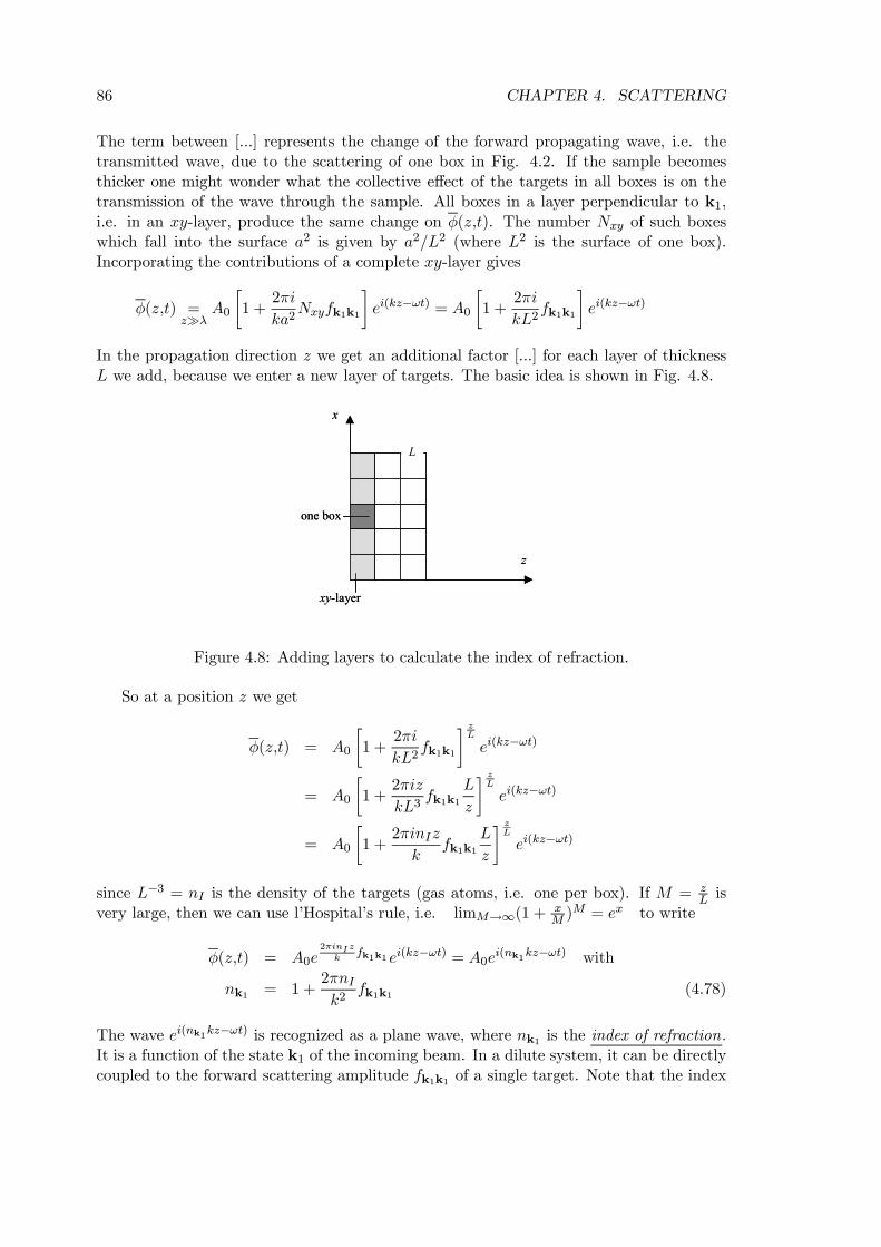
86 CHAPTER 4. SCATTERING
The term between [...] represents the change of the forward propagating wave, i.e. thetransmitted wave, due to the scattering of one box in Fig. 4.2. If the sample becomesthicker one might wonder what the collective effect of the targets in all boxes is on thetransmission of the wave through the sample. All boxes in a layer perpendicular to k1,i.e. in an xy-layer, produce the same change on φ(z,t). The number Nxy of such boxeswhich fall into the surface a2 is given by a2/L2 (where L2 is the surface of one box).Incorporating the contributions of a complete xy-layer gives
φ(z,t) =zÀλ
A0
·1 +
2πi
ka2Nxyfk1k1
¸ei(kz−ωt) = A0
·1 +
2πi
kL2fk1k1
¸ei(kz−ωt)
In the propagation direction z we get an additional factor [...] for each layer of thicknessL we add, because we enter a new layer of targets. The basic idea is shown in Fig. 4.8.
z
x
L
one box
xy-layer
z
x
L
one box
xy-layer
Figure 4.8: Adding layers to calculate the index of refraction.
So at a position z we get
φ(z,t) = A0
·1 +
2πi
kL2fk1k1
¸ zL
ei(kz−ωt)
= A0
·1 +
2πiz
kL3fk1k1
L
z
¸ zL
ei(kz−ωt)
= A0
·1 +
2πinIz
kfk1k1
L
z
¸ zL
ei(kz−ωt)
since L−3 = nI is the density of the targets (gas atoms, i.e. one per box). If M = zL is
very large, then we can use l’Hospital’s rule, i.e. limM→∞(1 + xM )
M = ex to write
φ(z,t) = A0e2πinIz
kfk1k1ei(kz−ωt) = A0ei(nk1kz−ωt) with
nk1 = 1 +2πnIk2
fk1k1 (4.78)
The wave ei(nk1kz−ωt) is recognized as a plane wave, where nk1 is the index of refraction.It is a function of the state k1 of the incoming beam. In a dilute system, it can be directlycoupled to the forward scattering amplitude fk1k1 of a single target. Note that the index
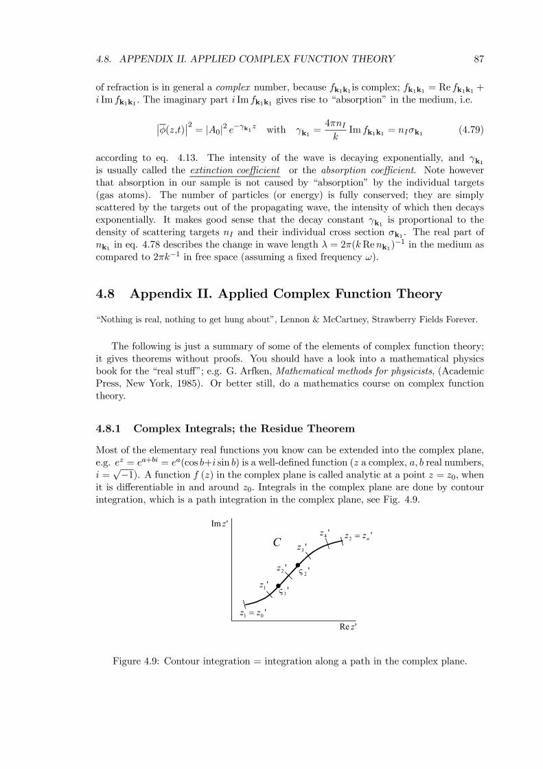
4.8. APPENDIX II. APPLIED COMPLEX FUNCTION THEORY 87
of refraction is in general a complex number, because fk1k1 is complex; fk1k1 = Re fk1k1 +i Im fk1k1 . The imaginary part i Im fk1k1 gives rise to “absorption” in the medium, i.e.
¯φ(z,t)
¯2= |A0|2 e−γk1z with γk1 =
4πnIk
Im fk1k1 = nIσk1 (4.79)
according to eq. 4.13. The intensity of the wave is decaying exponentially, and γk1is usually called the extinction coefficient or the absorption coefficient. Note howeverthat absorption in our sample is not caused by “absorption” by the individual targets(gas atoms). The number of particles (or energy) is fully conserved; they are simplyscattered by the targets out of the propagating wave, the intensity of which then decaysexponentially. It makes good sense that the decay constant γk1 is proportional to thedensity of scattering targets nI and their individual cross section σk1 . The real part ofnk1 in eq. 4.78 describes the change in wave length λ = 2π(kRenk1)
−1 in the medium ascompared to 2πk−1 in free space (assuming a fixed frequency ω).
4.8 Appendix II. Applied Complex Function Theory
“Nothing is real, nothing to get hung about”, Lennon & McCartney, Strawberry Fields Forever.
The following is just a summary of some of the elements of complex function theory;it gives theorems without proofs. You should have a look into a mathematical physicsbook for the “real stuff”; e.g. G. Arfken, Mathematical methods for physicists, (AcademicPress, New York, 1985). Or better still, do a mathematics course on complex functiontheory.
4.8.1 Complex Integrals; the Residue Theorem
Most of the elementary real functions you know can be extended into the complex plane,e.g. ez = ea+bi = ea(cos b+i sin b) is a well-defined function (z a complex, a, b real numbers,i =√−1). A function f (z) in the complex plane is called analytic at a point z = z0, when
it is differentiable in and around z0. Integrals in the complex plane are done by contourintegration, which is a path integration in the complex plane, see Fig. 4.9.
'Re z
'Im z
'01 zz =
'1z
'2z
'3z'4z '2 nzz =
'1ς
'2ς
C
Figure 4.9: Contour integration = integration along a path in the complex plane.
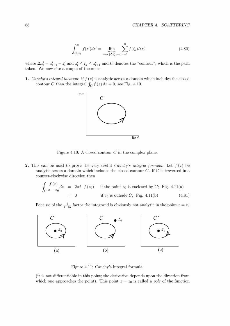
88 CHAPTER 4. SCATTERING
Z z2
C, z1
f(z0)dz0 = limn→∞
max |∆z0i|→0
nXi=1
f(ζi)∆z0i (4.80)
where ∆z0i = z0i+1 − z0i and z0i ≤ ζi ≤ z0i+1 and C denotes the “contour”, which is the path
taken. We now cite a couple of theorems
1. Cauchy’s integral theorem: if f (z) is analytic across a domain which includes the closedcontour C then the integral
HC f (z) dz = 0, see Fig. 4.10.
'Re z
'Im zC
Figure 4.10: A closed contour C in the complex plane.
2. This can be used to prove the very useful Cauchy’s integral formula: Let f (z) beanalytic across a domain which includes the closed contour C. If C is traversed in acounter-clockwise direction thenI
C
f (z)
z − z0dz = 2πi f (z0) if the point z0 is enclosed by C; Fig. 4.11(a)
= 0 if z0 is outside C; Fig. 4.11(b) (4.81)
Because of the 1z−z0 factor the integrand is obviously not analytic in the point z = z0
C
0z
C 0z C’
0z
(a) (b) (c)
Figure 4.11: Cauchy’s integral formula.
(it is not differentiable in this point; the derivative depends upon the direction fromwhich one approaches the point). This point z = z0 is called a pole of the function
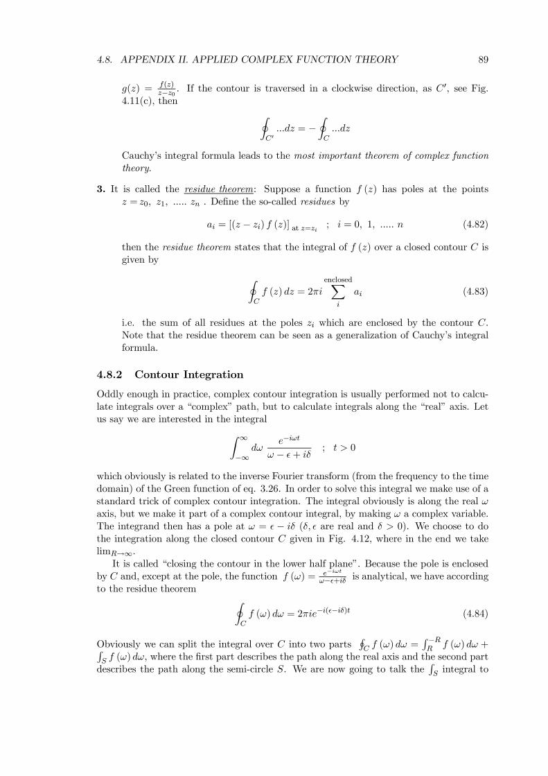
4.8. APPENDIX II. APPLIED COMPLEX FUNCTION THEORY 89
g(z) = f(z)z−z0 . If the contour is traversed in a clockwise direction, as C
0, see Fig.4.11(c), then I
C0...dz = −
IC...dz
Cauchy’s integral formula leads to the most important theorem of complex functiontheory.
3. It is called the residue theorem: Suppose a function f (z) has poles at the pointsz = z0, z1, ..... zn . Define the so-called residues by
ai = [(z − zi) f (z)] at z=zi ; i = 0, 1, ..... n (4.82)
then the residue theorem states that the integral of f (z) over a closed contour C isgiven by I
Cf (z) dz = 2πi
enclosedXi
ai (4.83)
i.e. the sum of all residues at the poles zi which are enclosed by the contour C.Note that the residue theorem can be seen as a generalization of Cauchy’s integralformula.
4.8.2 Contour Integration
Oddly enough in practice, complex contour integration is usually performed not to calcu-late integrals over a “complex” path, but to calculate integrals along the “real” axis. Letus say we are interested in the integralZ ∞
−∞dω
e−iωt
ω − ²+ iδ ; t > 0
which obviously is related to the inverse Fourier transform (from the frequency to the timedomain) of the Green function of eq. 3.26. In order to solve this integral we make use of astandard trick of complex contour integration. The integral obviously is along the real ωaxis, but we make it part of a complex contour integral, by making ω a complex variable.The integrand then has a pole at ω = ² − iδ (δ, ² are real and δ > 0). We choose to dothe integration along the closed contour C given in Fig. 4.12, where in the end we takelimR→∞.
It is called “closing the contour in the lower half plane”. Because the pole is enclosedby C and, except at the pole, the function f (ω) = e−iωt
ω−²+iδ is analytical, we have accordingto the residue theorem I
Cf (ω) dω = 2πie−i(²−iδ)t (4.84)
Obviously we can split the integral over C into two partsHC f (ω) dω =
R −RR f (ω) dω +R
S f (ω) dω, where the first part describes the path along the real axis and the second partdescribes the path along the semi-circle S. We are now going to talk the
RS integral to
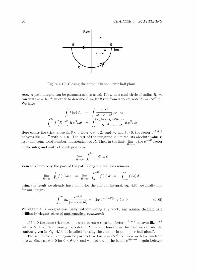
90 CHAPTER 4. SCATTERING
ωRe
ωIm
CRR−
δε i−
S
Figure 4.12: Closing the contour in the lower half plane.
zero. A path integral can be parametrized as usual. For ω on a semi-circle of radius R, wecan write ω = Reiθ; in order to describe S we let θ run from π to 2π; note dω = Reiθidθ.We have Z
Sf (ω) dω =
ZS
e−ωt
ω − ²+ iδdω orZ 2π
πf³Reiθ
´Reiθidθ =
Z 2π
π
etR sin θe−itR cos θ
Reiθ − ²+ iδ Reiθidθ
Here comes the trick: since sin θ < 0 for π < θ < 2π and we had t > 0, the factor etR sin θ
behaves like e−αR with α > 0. The rest of the integrand is limited, its absolute value isless than some fixed number, independent of R. Then in the limit lim
R→∞, the e−αR factor
in the integrand makes the integral zero
limR→∞
Z 2π
π... dθ = 0
so in this limit only the part of the path along the real axis remains
limR→∞
ICf (ω) dω = lim
R→∞
Z −R
Rf (ω) dω = −
Z ∞
−∞f (ω) dω
using the result we already have found for the contour integral, eq. 4.84, we finally findfor our integral Z ∞
−∞dω
e−iωt
(ω − ²+ iδ) = −2πie−i(²−iδ)t ; t > 0 (4.85)
We obtain this integral essentially without doing any work; the residue theorem is abrilliantly elegant piece of mathematical equipment!
If t < 0 the same trick does not work because then the factor etR sin θ behaves like eαR
with α > 0, which obviously explodes if R → ∞. However in this case we can use thecontour given in Fig. 4.13. It is called “closing the contour in the upper half plane”.
The semicircle S can again be parametrized as ω = Reiθ; but now we let θ run from0 to π. Since sin θ > 0 for 0 < θ < π and we had t < 0, the factor etR sin θ again behaves
4.8. APPENDIX II. APPLIED COMPLEX FUNCTION THEORY 91
ωRe
ωIm
CRR−
δε i−
S
Figure 4.13: Closing the contour in the upper half plane.
like e−αR with α > 0 so limR→∞
RS f (ω) dω = 0. However
HC f (ω) dω = 0 according to the
residue theorem, since the pole ²− iδ now lies outside the closed contour C and thusZ ∞
−∞dω
e−iωt
(ω − ²+ iδ) = 0 for t < 0 (4.86)
NOTE that the results of eqs. 4.85 and 4.86 can be used to prove that the inverseFourier transform of bG+0 (ω), cf. eq. 3.26, i.e.
bG+0 (t) = 1
2π
Z ∞
−∞dω bG+0 (ω)
is given by eq. 3.23. Note especially how the +iδ term in the denominator of the integrandin eq. 4.86 transforms into the Θδ (t) function of eq. 3.25. Thus the little δ takes care ofthe physical “causality” which was discussed around eq. 3.6. Had we taken a −iδ terminstead (δ > 0), then we would have a pole at ω = ² + iδ in the upper half plane. Thecontour integral over the lower half plane, which is appropriate for t > 0, then leads tozero, since the contour does not enclose the pole. However, closing the contour in theupper half plane, which is appropriate for t < 0, encloses the pole. The result of thiscontour integration isZ ∞
−∞dω
e−iωt
(ω − ²− iδ) = 0 for t > 0Z ∞
−∞dω
e−iωt
(ω − ²− iδ) = 2πie−i(²+iδ)t for t < 0 (4.87)
The Green function operator corresponding with eq. 3.26 using a −iδ instead of the +iδis bG−0 (ω). From the results above we conclude that its inverse Fourier transform bG−0 (t) isdifferent from zero only for t < 0. There seems to be little physics in such an non-causalfunction, but we will have a use for this Green function later on in the program.
We have to say something about limits now, which is a confusing subject. Up untilthe last paragraph we have used a finite number δ > 0. But, as stated in the main text atsome point we usually want to take limδ→0. Let us look again at the main example of this
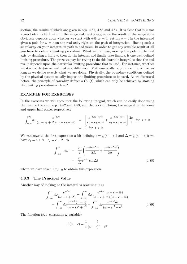
92 CHAPTER 4. SCATTERING
section, the results of which are given in eqs. 4.85, 4.86 and 4.87. It is clear that it is nota good idea to let δ → 0 in the integrand right away, since the result of the integrationobviously depends upon whether we start with +iδ or −iδ. Setting δ = 0 in the integrandgives a pole for ω = ² on the real axis, right on the path of integration. Having such asingularity on your integration path is bad news. In order to get any sensible result at allyou have to define a limiting procedure. What we did here, moving the pole off the realaxis by defining a finite δ, then do the integral and finally take limδ→0, is one well definedlimiting procedure. The prize we pay for trying to do this horrible integral is that the endresult depends upon the particular limiting procedure that is used. For instance, whetherwe start with +iδ or −iδ makes a difference. Mathematically, any procedure is fine, aslong as we define exactly what we are doing. Physically, the boundary conditions definedby the physical system usually impose the limiting procedure to be used. As we discussedbefore, the principle of causality defines a bG+0 (t), which can only be achieved by startingthe limiting procedure with +iδ.
EXAMPLE FOR EXERCISES
In the exercises we will encounter the following integral, which can be easily done usingthe residue theorem, eqs. 4.82 and 4.83, and the trick of closing the integral in the lowerand upper half plane, respectivelyZ ∞
−∞dω
e−iωt
(ω − ²1 + iδ) (ω − ²2 + iδ) =
"e−i(²1−iδ)t
²1 − ²2 + iδ +e−i(²2−iδ)t
²2 − ²1 + iδ
#2π
ifor t > 0
= 0 for t < 0
We can rewrite the first expression a bit defining ² = 12 (²1 + ²2) and ∆ =
12 (²1 − ²2); we
have ²1 = ²+∆ ²2 = ²−∆, soZ ∞
−∞...dω =
2π
i
Ãe−i(²+∆)t
−2∆ +e−i(²−∆)t
2∆
!=
2π
∆e−i²t sin∆t (4.88)
where we have taken limδ→0 to obtain this expression.
4.8.3 The Principal Value
Another way of looking at the integral is rewriting it asZ ∞
−∞dω
e−iωt
(ω − ²+ iδ) =Z ∞
−∞dω
e−iωt (ω − ²− iδ)(ω − ²+ iδ) (ω − ²− iδ)
=
Z ∞
−∞dωe−iωt (ω − ²)(ω − ²)2 + δ2
−Z ∞
−∞dω
e−iωtiδ(ω − ²)2 + δ2
(4.89)
The function (δ, ² constants; ω variable)
L(ω − ²) = 1
π
δ
(ω − ²)2 + δ2
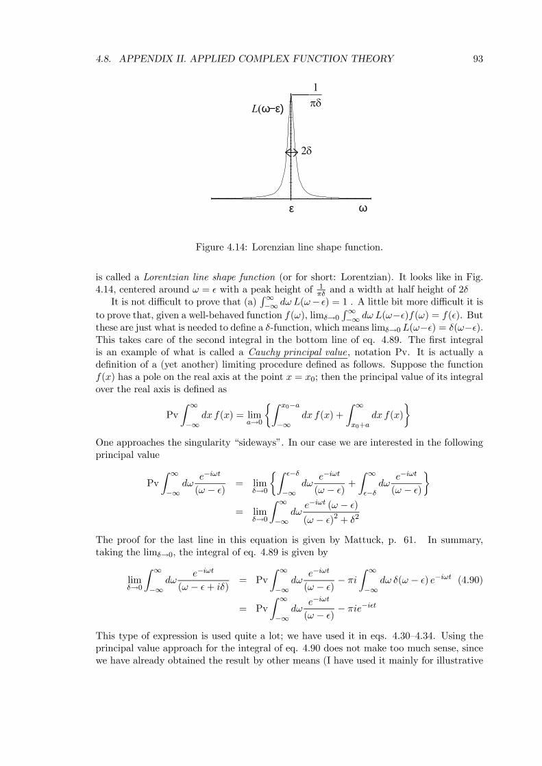
4.8. APPENDIX II. APPLIED COMPLEX FUNCTION THEORY 93
L(ω−ε)
ωε
πδ1
δ2
Figure 4.14: Lorenzian line shape function.
is called a Lorentzian line shape function (or for short: Lorentzian). It looks like in Fig.4.14, centered around ω = ² with a peak height of 1
πδ and a width at half height of 2δIt is not difficult to prove that (a)
R∞−∞ dωL(ω− ²) = 1 . A little bit more difficult it is
to prove that, given a well-behaved function f(ω), limδ→0R∞−∞ dωL(ω−²)f(ω) = f(²). But
these are just what is needed to define a δ-function, which means limδ→0 L(ω−²) = δ(ω−²).This takes care of the second integral in the bottom line of eq. 4.89. The first integralis an example of what is called a Cauchy principal value, notation Pv. It is actually adefinition of a (yet another) limiting procedure defined as follows. Suppose the functionf(x) has a pole on the real axis at the point x = x0; then the principal value of its integralover the real axis is defined as
Pv
Z ∞
−∞dx f(x) = lim
a→0
½Z x0−a
−∞dx f(x) +
Z ∞
x0+adx f(x)
¾One approaches the singularity “sideways”. In our case we are interested in the followingprincipal value
Pv
Z ∞
−∞dω
e−iωt
(ω − ²) = limδ→0
½Z ²−δ
−∞dω
e−iωt
(ω − ²) +Z ∞
²−δdω
e−iωt
(ω − ²)¾
= limδ→0
Z ∞
−∞dωe−iωt (ω − ²)(ω − ²)2 + δ2
The proof for the last line in this equation is given by Mattuck, p. 61. In summary,taking the limδ→0, the integral of eq. 4.89 is given by
limδ→0
Z ∞
−∞dω
e−iωt
(ω − ²+ iδ) = Pv
Z ∞
−∞dω
e−iωt
(ω − ²) − πi
Z ∞
−∞dω δ(ω − ²) e−iωt (4.90)
= Pv
Z ∞
−∞dω
e−iωt
(ω − ²) − πie−i²t
This type of expression is used quite a lot; we have used it in eqs. 4.30—4.34. Using theprincipal value approach for the integral of eq. 4.90 does not make too much sense, sincewe have already obtained the result by other means (I have used it mainly for illustrative
94 CHAPTER 4. SCATTERING
purposes). Comparison with eqs. 4.85 and 4.86 however does give the principal value ofthis particular integral
Pv
Z ∞
−∞dω
e−iωt
(ω − ²) = −πie−i²t for t > 0 (4.91)
= +πie−i²t for t < 0
We have used the function e−iωt in the numerator of the integrand as an example, but wecan replace it in eq. 4.90 by any well-behaved (real or complex) function f(ω) without aproblem.
I = limδ→0
Z ∞
−∞dω
f(ω)
(ω − ²+ iδ) = PvZ ∞
−∞dω
f(ω)
(ω − ²) − πi
Z ∞
−∞dω δ(ω − ²) f(ω) (4.92)
If the function f(ω) happens to be a real function, then PvR∞−∞ corresponds with the real
part of the integral Re I, and the δ-function part corresponds with Im I. Eq. 4.92 is oftenloosely written down as
limδ→0
1
ω − ²+ iδ =Pv
ω − ² − πiδ(ω − ²) (4.93)
It is called the well-known theorem from complex function theory .18 What is meant bythis odd short-hand notation is actually the full integral of eq. 4.92.
The integrals we have seen so far have been relatively simple. Often we encounterintegrals in which ²(k) with k a wave vector and we have to integrate over all wave vectorsin three dimensions, cf. eqs. 4.28— 4.34. Contour integration is not easy in that case andit becomes advantageous to use the separation in a Pv and a δ-function part. The latteris usually quite doable (although not as easy as in the one dimensional case); the Pv partrequires somewhat more work.
4.8.4 The Self-Energy Integral
In the text we have encountered an integral of the formZ ∞
−∞dω f (ω) =
Z ∞
−∞dω
e−iωt
ω − ²− Σ (ω)
where Σ (ω) = ReΣ (ω)+i ImΣ (ω) is a complex function, cf. eq. 4.37. Suppose ImΣ (ω) <0 and Σ (ω) is an analytical function. Furthermore suppose Σ (ω) is such that ω − ² −Σ (ω) = 0 has only one (complex) solution. Call that solution ω1. It is clear that theintegrand f (ω) has a pole at ω = ω1. As before, for t > 0 the integral can be done usingthe trick of closing the integral in the lower half plane and applying the residue theorem,eqs. 4.82 and 4.83. We need to calculate the residue
a1 = [(ω − ω1) f (ω)] at ω=ω1
18Calling something “well-known” is a well-known trick to intimidate the audience in order to avoidquestions that would embarasse the speaker.
4.8. APPENDIX II. APPLIED COMPLEX FUNCTION THEORY 95
Expand the analytical function Σ (ω) around ω = ω1
Σ (ω) = Σ (ω1) + Σ0 (ω1) (ω − ω1) +O
©(ω − ω1)
2ª
Then, using ²−Σ (ω1) = ω1
limω→ω1
(ω − ω1) f (ω) = limω→ω1
(ω − ω1) e−iωt
ω − ²− Σ (ω1)− Σ0 (ω1) (ω − ω1)−−O (ω − ω1)2= lim
ω→ω1
e−iωt
(1− Σ0 (ω1))−O (ω − ω1)1=
e−iω1t
1−Σ0 (ω1)
which finally gives for our integralZ ∞
−∞dω
e−iωt
ω − ²− Σ (ω) = −2πi e−iω1t
1−Σ0 (ω1) ; t > 0
= −2πie−i(Reω1−i|Imω1|)t
1−Σ0 (ω1) (4.94)
One observes that the factor (1− Σ0 (ω1))−1 corresponds to the factor zk in eq. 4.37. Notethat ω1 is a complex number and since ImΣ (ω) < 0 we also have Imω1 < 0; thus thisfactor leads to exponential decay. Of course for t < 0 one can prove by closing the contourin the upper half plane that the integral is zero.
In case |ImΣ (ω)| is very small, as one would expect for a quasi-particle, we can makea further approximation. Although as such this is not a part of complex analysis, thisapproximation is often done for quasi-particles and we will discuss it here. One startsfrom the equation for the pole
ω − ²− Σ (ω) = 0⇔ω − ²− ΣR (ω)− iΣI (ω) = 0
where ΣR (ω) ≡ ReΣ (ω) and ΣI (ω) ≡ ImΣ (ω). Denote ω = ω0 the (real) solution toω − ² − ΣR (ω) = 0. Because |ΣI (ω)| is small, the solution ω = ω1 of the pole equationwill be close to ω0. Make the following approximations
ΣI (ω) ≈ ΣI (ω0) (4.95)
ΣR (ω) ≈ ΣR (ω0) + Σ0R (ω0) (ω − ω0)
the pole equation becomes
ω − ²− ΣR (ω0)−Σ0R (ω0) (ω − ω0)− iΣI (ω0) = 0⇔ω − ω0 − Σ0R (ω0) (ω − ω0)− iΣI (ω0) = 0⇔
ω − ω0 =iΣI (ω0)
1− Σ0R (ω0)
96 CHAPTER 4. SCATTERING
or
ω1 = ω0 − i2Γ0 where
ω0 = ²+ΣR (ω0) and Γ0 =2 |ΣI (ω0)|1− Σ0R (ω0)
(4.96)
Consistent with the approximation of eq. 4.95 is using Σ0 (ω1) ≈ Σ0R (ω0) in eq. 4.94Z ∞
−∞dω
e−iωt
ω − ²− Σ (ω) = −2πie−i(ω0−
i2Γ0)t
1− Σ0R (ω0); t > 0 (4.97)
This equation is an approximation of eq. 4.94 when |ΣI (ω)| (or Γ0) is small.
Part II
Many Particles
97

Chapter 5
Quantum Field Oscillators
“Make everything as simple as possible, but not simpler”, A. Einstein.
In the previous chapter, we assumed that we could easily obtain all the eigenstatesof an unperturbed Hamiltonian bH0 . However, you already know from previous encoun-ters with quantum mechanics that in practice this is rare. Especially when dealing witha many particle system (and here few is already many) the best we can hope for is tofind decent approximations. Choosing the right representation (i.e. basis set) helps a lot.This is discussed in Mattuck’s Appendix A; you might want to check out this appendix.This chapter and the next one contain a few many particle systems that can be solved“exactly”. As we will see, all of these examples can be rewritten in terms of “indepen-dent”, i.e. non-interacting, particles. Sometimes this becomes clear only after choosingthe right representation. It will be illustrated in this chapter on a couple of many bosonproblems which are related to the ubiquitous harmonic oscillator. We will introduce therepresentation which is most widely used in many particle physics; it is called the occu-pation number representation. The techniques developed for handling this representationare called second quantization. This chapter is organized as follows. After learning theart of “solving the harmonic oscillator problem by algebra only”, this art is then appliedto the problem of lattice dynamics. The continuum limit of the lattice problem serves toillustrate how to quantize a classical system which is described by a field, and not by acollection of mechanical particles. In the last section I briefly discuss the quantization ofthe classical electro-magnetic field using this method. In general, quantizing a classicalfield using the second quantization technique (or occupation number representation) is thesubject of quantum field theory.
5.1 The Quantum Oscillator
The harmonic oscillator is a true work horse both in quantum as well as in classical me-chanics. In this section I will reproduce the all-time-number-one of the quantum mechanicscharts; “how to solve the harmonic oscillator problem with just a bit of operator algebra”.In one dimension the Hamiltonian of the harmonic oscillator is given by
bH =bp22m
+1
2mω2bx2 (5.1)
99
100 CHAPTER 5. QUANTUM FIELD OSCILLATORS
In order to get rid of the clumsy constants we rescale the operators
bP = (m~ω)−12 bp and bQ = ³mω
~
´ 12 bx (5.2)
The Hamiltonian then gets the simple form
bH =1
2
³ bP 2 + bQ2´ ~ω (5.3)
From the fundamental commutation relation [bx, bp] = i~ one obtainsh bQ, bPi = i (5.4)
Eqs. 5.3 and 5.4 are sufficient to find the eigenvalues and eigenstates of bH by a simplebit of algebra. The first step is to define an operator
ba = 1√2
³ bQ+ i bP´ (5.5)
from which it follows, since bQ and bP are Hermitian operators,ba† = 1√
2
³ bQ− i bP´Note that ba 6= ba†, so this operator is not an observable. From the commutation relation,eq. 5.4, it is easy to provehba,ba†i =
1
2
nh bQ, bQi+ i h bP, bQi− i h bQ, bPi+ h bP, bPio=
1
20 + i ·−i− i · i+ 0 = 1
Furthermore
ba†ba = 1
2
n bQ2 − i bP bQ+ i bQ bP + bP 2o = 1
2
³ bP 2 + bQ2´+ i
2
h bQ, bPiThe Hamiltonian eqs. 5.3 is then rewritten using eq. 5.4 as
bH =
µba†ba+ 12
¶~ω (5.6)hba,ba†i = 1 (5.7)
These are the two equations we need. For instance, it is easy to show thath bH,bai =n³ba†ba´ba− ba³ba†ba´o~ω
=n³baba† − 1´ba− ³baba†´bao ~ω = −ba~ω
(the constant 12 in the Hamiltonian commutates with everything). From this it follows
that bHba = ba³ bH − ~ω´ (5.8)
5.1. THE QUANTUM OSCILLATOR 101
Here jumps the rabbit out of the high hat. Let |νi be an eigenstate of bH, i.e. bH|νi = ²ν |νi,then ba|νi is also an eigenstate of bH with eigenvalue ²ν − ~ω, since
bHba|νi = ba³ bH − ~ω´ |νi = ba (²ν − ~ω) |νi = (²ν − ~ω)ba|νi (5.9)
By repeatedly applying ba we can now step down the eigenvalue ladder, i.e. ban|νi is aneigenstate of bH with eigenvalue ²ν − n~ω; simply repeat the rule given by eq. 5.8. Thisfalling down the ladder has to stop for some value of n, when we arrive at the bottom ofthe ladder, at the ground state. Moreover, the eigenvalue ²ν − n~ω has to stay positiveand ≥ 1
2~ω
Proof: Call ban|νi = |ν0i, ²ν − n~ω = ²ν0 , bH|ν0i = ²ν0 |ν0i. Then ba†ba|ν0i =³ bH~ω − 1
2
´|ν0i = ¡ ²ν0~ω − 1
2
¢ |ν0i ≡ bν0 |ν0i, according to eq. 5.6. Also hν0|ba†ba|ν0i = bν0hν 0|ν0i.On the other hand hν0|ba†ba|ν0i = hbaν 0|baν0i = kba|ν 0ik2 > 0, because the norm of thevector ba|ν0i always has to be positive (one of the axiom’s of an inner product space).Since hν 0|ν0i > 0 by the same rule, we therefore conclude that bν0 > 0, or in other words²ν0 >
12~ω. The only exception is if |ν0i = |i, the “null” vector of the vector space, for which
h|i = 0. We can repeat the trick with |ν00i = ban−1|νi and, knowing that ba|ν00i = |ν 0i = |i,we have ba†ba|ν00i = ³ bH
~ω − 12
´|ν00i = ¡ ²ν00~ω − 1
2
¢ |ν00i = |i or ²ν00 = 12~ω.
In conclusion, the only way to end falling down the eigenvalue ladder by repeatedapplication of the step-down operator ba is to have some power m of ba giving the “null”vector |i, i.e.
bam|νi = |i (5.10)
(Note this then holds for any power n ≥ m by elementary linear algebra, since any linearoperation maps the null vector onto itself, bA|i = |i). The last power (m−1) which doesn’tgive the null vector must be the ground state |0i = bam−1|νi. According to the proof givenabove its eigenvalue must be 12~ω. From this ground state |0i we can step up the eigenvalueladder again, using the step-up operator ba†. Analogous to eq. 5.8, we can prove
bHba† = ba† ³ bH + ~ω´
so
bHba†|0i = µ12+ 1
¶~ωba†|0i
and
bH ³a†´n |0i = µn+ 12
¶~ω³ba†´n |0i ; n = 1, 2, .... (5.11)
We have found a way to construct all the eigenstates of the harmonic oscillator (ponder abit about why we find all the eigenstates this way). The only remaining thing we have totake care of is normalization, because we like our eigenstates normalized. This we do in thefollowing way. Suppose |ni, the eigenstate with eigenvalue ²n =
¡n+ 1
2
¢~ω is normalized,
then ba|ni = cn|n−1i steps down the ladder with cn a constant to be determined. Its norm
102 CHAPTER 5. QUANTUM FIELD OSCILLATORS
is, using eq. 5.7, hban|bani = n|ba†ba|n® = hn| bH~ω − 12 |ni = n hn|ni = n, since by assumption
|ni was normalized. However, we also have hban|bani = |cn|2 hn− 1|n− 1i = n. So if wechoose cn =
√n, the vector |n− 1i is also normalized.1 In other words
ba|ni = √n|n− 1i (5.12)
In a similar way we can prove
a†|ni = √n+ 1|n+ 1i (5.13)
Using eq. 5.13 we can climb the eigenstate ladder step by step
|1i =1√1ba†|0i ; |2i = 1√
2ba†|1i = 1√
2.1
³ba†´2 |0i ;|3i =
1√3ba†|2i = 1√
3.2
³ba†´2 |1i = 1√3.2.1
³ba†´3 |0iIn general, all the eigenstates of the Harmonic oscillator can be expressed as
|ni =¡a†¢n
√n!|0i (5.14)
If we start with a normalized ground state |0i then all the states are normalized.
5.1.1 Summary Harmonic Oscillator
The Hamiltonian is given by
bH =bp22m
+1
2mω2bx2 = 1
2
³ bP 2 + bQ2´ ~ωwhere
bP = (m~ω)− 12 bp bQ = ³mω
~
´ 12 bx
define
ba = 1√2
³ bQ+ i bP´ ba† = 1√2
³ bQ− i bP´then we can rewrite the Hamiltonian as
bH =
µ1
2+ ba†ba¶~ω
hba,ba†i = 11We might add a phase factor, i.e. cn = eiαn
√n ; αn arbitrary. The resulting vector would still be
normalized. We take the liberty to set αn = 0;∀n
5.1. THE QUANTUM OSCILLATOR 103
Using only operator algebra we have found that all the eigenstates of bH can be labeledby a natural number n, for which
bH|ni = ²n|ni ; n = 0, 1, 2, .....the eigenvalues are given by
²n =
µn+
1
2
¶~ω
The operators ba and ba† can be used to step-down and step-up the eigenvalue ladder,respectively
ba|ni = √n|n− 1i ba†|ni = √n+ 1|n+ 1iIn fact, starting from the ground state |0i we can step-up the whole ladder
|ni =¡ba†¢n√n!|0i
5.1.2 Second Quantization
It is tempting to interpret the eigenstates |ni and their energies ²n =¡n+ 1
2
¢~ω in the
following way:
• The state |ni contains n identical quanta, each with energy ~ω.• The operator ba†, which increases n by 1, creates an additional quantum and is thuscalled creation operator . Similarly ba is the annihilation operator since it annihilatesa quantum.
• The operator bN = ba†ba is called the number operator sincebN |ni = ba†ba|ni = n 1
2ba†|n− 1i = n|niit counts the number of quanta of the state |ni
• The state |0i has no quanta, it is called the vacuum state (or vacuum for short).Don’t confuse it with the null vector; the state |0i is the ground state of the system,and thus a non-trivial vector.
• All states can be created by letting the creation operator repeatedly operate on thevacuum to create quanta of energy ~ω.
The language of ba,ba†, |ni etcetera, is called the language of second quantization. Theidea is that writing down the Hamiltonian, eq. 5.1, as a quantum operator is “firstquantization”. The language of first quantization can be translated into wave mechanicsusing the position representation. The interpretation of the eigenstates of the Hamiltonianas being composed of n individual but identical quanta is then “second quantization”.Since |ni contains n quanta, a representation using |ni; n = 0, 1, 2, .... as a basis set iscalled the number representation (or also the occupation number representation). It is
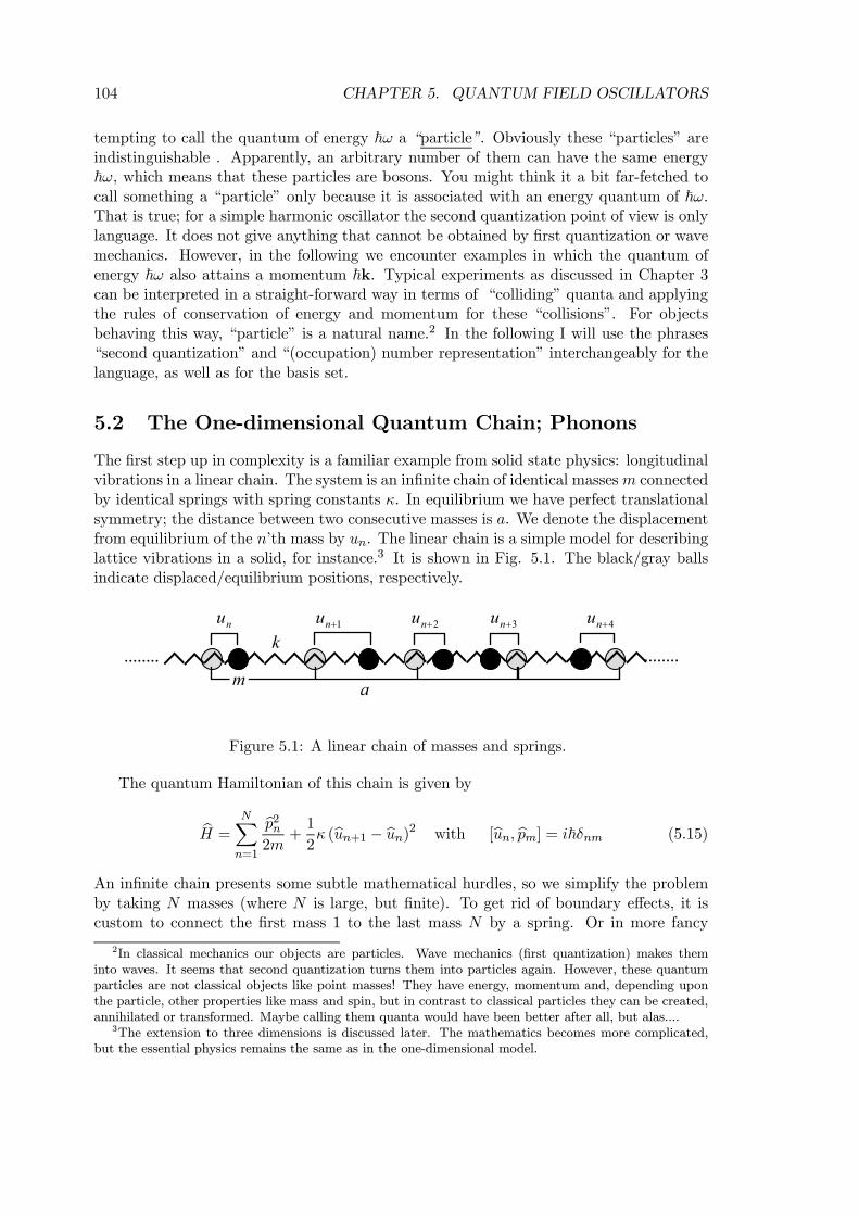
104 CHAPTER 5. QUANTUM FIELD OSCILLATORS
tempting to call the quantum of energy ~ω a “particle”. Obviously these “particles” areindistinguishable . Apparently, an arbitrary number of them can have the same energy~ω, which means that these particles are bosons. You might think it a bit far-fetched tocall something a “particle” only because it is associated with an energy quantum of ~ω.That is true; for a simple harmonic oscillator the second quantization point of view is onlylanguage. It does not give anything that cannot be obtained by first quantization or wavemechanics. However, in the following we encounter examples in which the quantum ofenergy ~ω also attains a momentum ~k. Typical experiments as discussed in Chapter 3can be interpreted in a straight-forward way in terms of “colliding” quanta and applyingthe rules of conservation of energy and momentum for these “collisions”. For objectsbehaving this way, “particle” is a natural name.2 In the following I will use the phrases“second quantization” and “(occupation) number representation” interchangeably for thelanguage, as well as for the basis set.
5.2 The One-dimensional Quantum Chain; Phonons
The first step up in complexity is a familiar example from solid state physics: longitudinalvibrations in a linear chain. The system is an infinite chain of identical massesm connectedby identical springs with spring constants κ. In equilibrium we have perfect translationalsymmetry; the distance between two consecutive masses is a. We denote the displacementfrom equilibrium of the n’th mass by un. The linear chain is a simple model for describinglattice vibrations in a solid, for instance.3 It is shown in Fig. 5.1. The black/gray ballsindicate displaced/equilibrium positions, respectively.
nu 1+nu 2+nu 3+nu 4+nu
am
k
Figure 5.1: A linear chain of masses and springs.
The quantum Hamiltonian of this chain is given by
bH =NXn=1
bp2n2m
+1
2κ (bun+1 − bun)2 with [bun, bpm] = i~δnm (5.15)
An infinite chain presents some subtle mathematical hurdles, so we simplify the problemby taking N masses (where N is large, but finite). To get rid of boundary effects, it iscustom to connect the first mass 1 to the last mass N by a spring. Or in more fancy
2In classical mechanics our objects are particles. Wave mechanics (first quantization) makes theminto waves. It seems that second quantization turns them into particles again. However, these quantumparticles are not classical objects like point masses! They have energy, momentum and, depending uponthe particle, other properties like mass and spin, but in contrast to classical particles they can be created,annihilated or transformed. Maybe calling them quanta would have been better after all, but alas....
3The extension to three dimensions is discussed later. The mathematics becomes more complicated,but the essential physics remains the same as in the one-dimensional model.
5.2. THE ONE-DIMENSIONAL QUANTUM CHAIN; PHONONS 105
terms, one applies periodic boundary conditions, i.e. buN+1 = bu1, etcetera. This trick issimilar to the one we used in Section 4.2; in the end we can always take limN→∞. Werewrite the Hamiltonian a bit using (bun+1 − bun)2 = bu2n + bu2n+1 − 2bunbun+1. Since we haveapplied periodic boundary conditions it follows that
Pn bu2n =Pn bu2n+1 (the sums are over
all masses). Defining
ω0 =
r2κ
m(5.16)
we get the form
bH =NXn=1
bp2n2m
+1
2mω20
µbu2n − 12bunbun+1 − 12bun+1bun¶
(5.17)
Since bun+1 and bun commutate: [bui, buj ] = 0 and [bpi, bpj ] = 0 ∀i,j , we may freely interchangetheir order. I prefer to use this symmetric form. You have solved this problem a couple oftimes before in classical mechanics and solid state physics, where it leads to normal modesand phonons. As a quantum problem, it is our first many body problem. In principle, onecould try and solve this problem head-on in the position representation. We then need awave function Φ that keeps track of the positions un of all the N masses involved. Asusual we would set bpn → ~
i∂
∂un; bun → un and the Schrodinger equation becomes"
NXn=1
− ~2
2m
∂2
∂u2n+1
2mω20
µu2n −
1
2unun+1 − 1
2un+1un
¶#Φ (u1, u2, u3,......, uN−1, uN , t)
= i~∂
∂tΦ (u1, u2, u3,......, uN−1, uN , t) (5.18)
Needless to say that blindly trying to solve this N -dimensional differential equation is ahopeless exercise, even on a computer (unless N is small).
We can however reformulate the problem in terms of a new set of particles, calledphonons. As by magic, our many-body problem will decouple into a set of one-particleproblems.4 Each phonon will involve all the old particles of Fig. 5.1. In some booksthe phonon is called a collective excitation; others call it a quasi-particle, analogous tothe term used in Chapter 4. Here is how the mathematics goes; we define new operatorsbpk, bqk
bpk` =1√N
N−1Xn=0
e−ik`nabpnbqk` =
1√N
N−1Xn=0
e−ik`nabun (5.19)
where k` = `2πNa ; ` = 0, 1....N − 1 and a is equilibrium distance between masses, see Fig.
5.1. You will recognize this as a discrete Fourier transform. Using the familiar relations
4Of course, magic has very little to do with it. We use a transformation which decouples a many coupledharmonic oscillator problem into uncoupled normal mode oscillations, as in classical mechanics.
106 CHAPTER 5. QUANTUM FIELD OSCILLATORS
for discrete Fourier transforms
N−1Xn=0
ei(k−k0)na = Nδk,k0
N−1X`=0
eik`(n−n0)a = Nδn,n0 (5.20)
we can invert the relations of eq. 5.19
bun =1√N
N−1X`=0
eik`nabqk`bpn =
1√N
N−1X`=0
eik`nabpk` (5.21)
The Hamiltonian of eq. 5.17 can be rewritten as (dropping the ` subscripts, and using anotation where k denotes one of the allowed k` values)
bH =Xk
bp†kbpk2m
+1
2mω20 bq†kbqk µ1− 12eika − 12e−ika
¶(5.22)
Since 12eika + 1
2e−ika = cos ka and defining
ω (k) = ω0 (1− cos ka)12 = 2
rκ
m| sin 1
2ka| (5.23)
we can write
bH =Xk
bp†kbpk2m
+1
2mω (k)2 bq†kbqk (5.24)
Comparing this to eq. 5.1 we see that it is in fact a sum of independent harmonic oscilla-tors, each labeled by k, with a characteristic frequency given by ω (k). Since bqk`+N = bqk`and bpk`+N = bpk` , cf. eq. 5.19 we have a periodicity also in k space. We have somefreedom in choosing the interval over which we let the independent k` = `
2πNa run. In solid
state physics it is custom to use ` = −N2 + 1, ....., N2 , such that −π
2 < k ≤ π2 ; this defines
the so-called Brillouin zone.5 The relation between the frequency ω of an oscillator andk (which turns out to be a wave number) is called a dispersion relation. The one givenby eq. 5.23 is shown in Fig. 5.2 (assuming that N is very large, so we may plot it as acontinuous function).
We have solved the harmonic oscillator in the previous section; nothing much changessince all the oscillators are independent. We can work through it again, and add an index
5Had we chosen as our interval k0`; ` = 0, 1....N − 1 then 0 ≤ k0 < 2π. Because of the periodicity in kspace the index k0` would run over the same values as the index k`, and the physical results would be thesame. We prefer the more symmetric interval −π
2< k ≤ π
2.
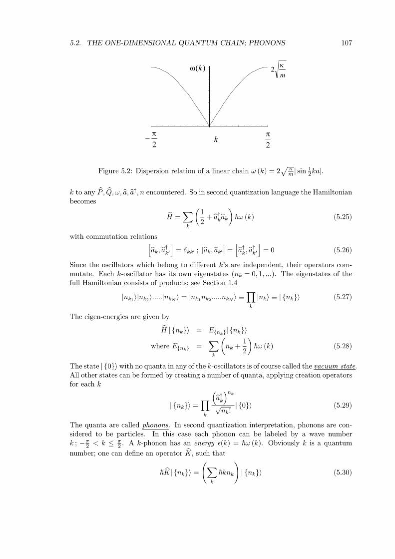
5.2. THE ONE-DIMENSIONAL QUANTUM CHAIN; PHONONS 107
2π
2π
− k
)(kωmκ2
Figure 5.2: Dispersion relation of a linear chain ω (k) = 2p
κm | sin 12ka|.
k to any bP, bQ,ω,ba,ba†, n encountered. So in second quantization language the Hamiltonianbecomes
bH =Xk
µ1
2+ ba†kbak¶~ω (k) (5.25)
with commutation relationshbak,ba†k0i = δkk0 ; [bak,bak0 ] = hba†k,ba†k0i = 0 (5.26)
Since the oscillators which belong to different k’s are independent, their operators com-mutate. Each k-oscillator has its own eigenstates (nk = 0, 1, ...). The eigenstates of thefull Hamiltonian consists of products; see Section 1.4
|nk1i|nk2i.....|nkN i = |nk1nk2 .....nkN i ≡Yk
|nki ≡ | nki (5.27)
The eigen-energies are given bybH | nki = Enk| nki
where Enk =Xk
µnk +
1
2
¶~ω (k) (5.28)
The state | 0i with no quanta in any of the k-oscillators is of course called the vacuum state.All other states can be formed by creating a number of quanta, applying creation operatorsfor each k
| nki =Yk
³ba†k´nk√nk!
| 0i (5.29)
The quanta are called phonons. In second quantization interpretation, phonons are con-sidered to be particles. In this case each phonon can be labeled by a wave numberk ; −π
2 < k ≤ π2 . A k-phonon has an energy ²(k) = ~ω (k). Obviously k is a quantum
number; one can define an operator bK, such that~ bK| nki = ÃX
k
~knk
!| nki (5.30)
108 CHAPTER 5. QUANTUM FIELD OSCILLATORS
One can also define operators bk1,bk2, ....bkn operating on a single k-phonon state, i.e.~bk1|nk1i = ~k1nk1 |nk1i etcetera. Obviously one hasbK = bk1 + bk2.....+ bkN =X
k
bk (5.31)
Analyzing processes in which phonons interact with other particles like neutrons, electrons,or photons, we can assign to each phonon a momentum p = ~k. (We will discuss this inmore detail later on). The operator ~bk is then the momentum operator for k-phonons;~ bK is the total momentum operator. In contrast to the simple harmonic oscillator inSection 5.1, the quanta (phonons) of the chain have a well-defined momentum as well asan energy; reason enough to call them particles. Pnk = hnk |~ bK| nki = P
k ~knkis obviously the total momentum of the state | nki. One can easily check that thestates | nk (t)i = exp(− i
~Enk)| nki with the total energy Enk are solutions of theSchrodinger equation
i~∂
∂t| nk (t)i = bH| nk (t)i
So by choosing a convenient representation, the occupation number representation, we havebeen able to solve the Schrodinger equation in a fairly straight-forward way and avoid theproblems, had we tried to solve the same equation in the position representation, see eq.5.18.6
5.3 My First Quantum Field
“Het gaat altijd om tijd en ruimte. Dus moet je zorgen dat het middenveld goed in evenwicht is”,
J. Cruijff over veldentheorie. (“The key issues are always time and space. Thus you have to make
sure that the midfield is always well-balanced”, the Dutch philosopher J. Cruijff on field theory.)
In the foregoing section we extended the techniques developed for the single quantumharmonic oscillator in Section 5.1 to the case of many coupled harmonic oscillators. Themost important trick was the transformation of eq. 5.19; from there on the system de-coupled into simple harmonic oscillators again. Imagine that the masses are not pointmasses like in Fig. 5.1, but they are spread out in a uniform way and constitute an elasticmedium. Each mass element of the medium can have a displacement from its equilibriumposition. The displacement u does not any longer depend upon a discrete index i, which isassociated with discrete (point) masses, but it depends upon a continuous variable, namelythe position x along the chain, i.e. u(x). A continuous physical function like u(x) is calleda field. The position x labels the degrees of freedom of the system. A field thus has aninfinite, continuous set of degrees of freedom, in contrast to the discrete chain, where imight run to infinity, but at least you can count the degrees of freedom one by one. Anartists impression of the displacement field is given in Fig. 5.3.
We want to give a quantum mechanical description of a field. Since the “infinities” ofa field are a bit tricky to handle mathematically, I will develop the theory of the classicalfield of the elastic medium first, before I come to the quantum field description.
6If you really want to, it is possible to construct wave functions from the states | nki. It would involveHermite polynomials, etcetera, familiar to you from elementary quantum mechanics. However, this wouldnot add anything new to the physics. On the contrary, it makes things less transparent.
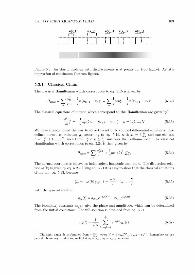
5.3. MY FIRST QUANTUM FIELD 109
( )nu x 1( )nu x + 2( )nu x + 3( )nu x + 4( )nu x +( )nu x 1( )nu x + 2( )nu x + 3( )nu x + 4( )nu x +( )nu x 1( )nu x + 2( )nu x + 3( )nu x + 4( )nu x +
Figure 5.3: An elastic medium with displacements u at points xm (top figure). Artist’simpression of continuum (bottom figure).
5.3.1 Classical Chain
The classical Hamiltonian which corresponds to eq. 5.15 is given by
Hclass =Xn
p2n2m
+1
2κ (un+1 − un)2 =
Xn
1
2mu2n +
1
2κ (un+1 − un)2 (5.32)
The classical equations of motion which correspond to this Hamiltonian are given by7
d2undt2
= −12ω20 (2un − un+1 − un−1) ; n = 1, 2, ..., N (5.33)
We have already found the way to solve this set of N coupled differential equations. Onedefines normal coordinates qk` according to eq. 5.19, with k` = ` 2πNa and one chooses` = −N
2 + 1, ......N2 , such that −π2 < k ≤ π
2 runs over the Brillouin zone. The classicalHamiltonian which corresponds to eq. 5.24 is then given by
Hclass =Xk
p∗kpk2m
+1
2mω (k)2 q∗kqk (5.34)
The normal coordinates behave as independent harmonic oscillators. The dispersion rela-tion ω (k) is given by eq. 5.23. Using eq. 5.21 it is easy to show that the classical equationsof motion, eq. 5.33, become
qk` = −ω (k) qk` ; ` =−N2+ 1, ......
N
2(5.35)
with the general solution
qk`(t) = ak`,0e−iω(k)t + ak`,1e
iω(k)t (5.36)
The (complex) constants ak`,0;1 give the phase and amplitude, which can be determinedfrom the initial conditions. The full solution is obtained from eq. 5.21
un(t) =1√N
N2X
`=−N2+1
eik`naqk`(t) (5.37)
7The right handside is obtained from − ∂V∂un
, where V = 14mω20
Pn (un+1 − un)2. Remember we use
periodic boundary conditions, such that u0 = uN ; u1 = uN+1, etcetera
110 CHAPTER 5. QUANTUM FIELD OSCILLATORS
Obviously these displacements have to be real numbers, i.e. u∗n = un, from which onederives the relation ak`,1 = a
∗−k`,0, so eq. 5.36 becomes
qk`(t) = ak`,0e−iω(k)t + a∗−k`,0e
iω(k)t (5.38)
Each k` labels a so-called normal mode of the chain (or simply mode for short).8 Thedisplacements ui of all the masses along the chain in case only a single (normal) mode isexcited can be found by setting qk`(t) = 0 for all k` except one. One then obtains wave-likedisplacement pattern eik`iaqk`(t) and the most general solution is a linear combination ofsuch waves. One reserves the name normal mode for the spatially dependent part eik`na;the (harmonic) time-dependent qk`(t) part incorporates the phase and amplitude of thewave.
5.3.2 Continuum Limit: an Elastic Medium
We now take the continuum limit of this system. Imagine that the masses are not pointmasses like in Fig. 5.1, but that they are spread out, like in Fig. 5.3. In equilibrium wehave a constant mass density µ = m/a. We denote the position of a mass element along thecontinuous chain by x. Each mass element can have a displacement. The displacementu does not any longer depend upon a discrete index n, which is associated with pointmasses, but it becomes a variable u(x), which depends continuously upon the positionalong the chain x. In the discrete case u is only defined for the discrete set of pointsxn = na ; n = 1, 2..., N ; i.e. u(xn) = un. A continuous physical variable like u(x) is calleda field, and since we are doing classical mechanics for the moment, it is a classical field.The equation of motion which governs this classical field is easily obtained by taking thecontinuum limit of eq. 5.33. One uses on the right handside
−[2un − un+1 − un−1] = [un+1 − un]− [un − un−1] =
[u(xn+1)− u(xn)]− [u(xn)− u(xn−1)] = a2(u(xn+a)−u(xn)
a − u(xn)−u(xn−a)a
a
)
The expression between is recognized as the discrete approximation to the secondderivative ∂2u(x)
∂x2and the latter is obtained by taking the continuum limit lima→0 of this
expression. The prefactor on the right handside of eq. 5.33 now is (aω0)2. For discrete
point masses we defined ω0 =p2κ/m by eq. 5.16. The spring constant κ of a spring scales
with its length a as κ = τ/a with τ a constant determined by the materials properties ofthe spring, which is called the “elasticity” or “tension”of the spring. With a mass densityµ = m/a we can write ω0 =
1a
p2τ/µ. Now define the constant v0 = aω0 or
v0 =p2τ/µ (5.39)
in terms of the materials properties of the continuum. Note that v0 has the dimension of
velocity (m/s) =£kgm/s2 ·m/kg¤ 12 . The continuum limit of eq. 5.33 thus becomes
∂2u(x, t)
∂t2= v20
∂2u(x, t)
∂x2(5.40)
8We absorbed the prefactor 1√Ninto the phase/amplitude factors ak`,0.
5.3. MY FIRST QUANTUM FIELD 111
The time and position dependence of the displacement field of a continuous chain thusobeys a wave equation. The continuous chain is of course nothing else than a homogeneouselastic medium, and eq. 5.37 describes the elastic waves (or sound waves). The constantv0 is the speed of sound in the medium. The general solution of the wave equation can befound by taking the continuum limit of eq. 5.37. We use a trick similar to eq. 4.28; thespacing between our discrete k values was ∆k = 2π
L , where L = Na is the total length ofthe medium. We take L large such that ∆k becomes small enough to take the integralX
k
... =1
∆k
Xk
...∆k −→ L
2π
Z...dk
Incorporating the prefactor into a normalization constant N to be determined later on,we get as the general solution of the wave equation
u(x, t) = NZ ∞
−∞eikxq(k, t)dk (5.41)
where, according to eq. 5.38
q(k, t) = a(k)eiω(k)t + a(−k)∗e−iω(k)t (5.42)
We recognize as a continuous superposition of waves. As usual, the phases and amplitudesa(k) (now a function of the wave number k), are determined by initial conditions. Againthe name mode or normal mode is reserved for the spatial dependent part eikx. Thefunction q(k, t) replaces the collection of amplitudes and phases of the discrete case; onecan also say that since we have an infinite system, there are infinite degrees of freedomwhich can be labeled by k. Trying out eq. 5.41 in eq. 5.37 givesZ ∞
−∞(±iω (k))2eikxq(k, t)dk = v20
Z ∞
−∞(ik)2eikxq(k, t)dk
In order that this is true for any a(k) we must have the following dispersion relation
ω (k) = v0k (5.43)
The constant v0 thus determines the speed at which the sound waves travel, as we haveforeseen. The total energy H for the discrete chain is given by
H =Xn
1
2mu2n +
1
2κ (un+1 − un)2
We use the by now familiar tricks to go to the continuum limit. The spacing between thelattice sites n was ∆x = a. Use
Pn ... =
1a
Pn ...∆x and un+1− un = a(u(xn+a)−u(xn)a )→
a∂u(x)∂x . Furthermore, use the definitions of mass density µ = m/a and elasticity τ = κaand transform the sum
Pn ...∆x into an integral
R...dx
H =
Z ∞
−∞dx
"1
2µ
µ∂u(x, t)
∂t
¶2+1
2τ
µ∂u(x, t)
∂x
¶2#(5.44)
112 CHAPTER 5. QUANTUM FIELD OSCILLATORS
This is the classical energy of an elastic medium of length L. The expression can betransformed to an integral over k by using of eq. 5.41. For instance, defining q(k, t) =∂q(k,t)
∂tZ ∞
−∞dx
∂u(x, t)
∂t
∂u(x, t)
∂t= N 2
Z ∞
−∞dx
Z ∞
−∞eikxq(k, t)dk ·
Z ∞
−∞eik
0xq(k0, t)dk0
= N 2
Z ∞
−∞dk0 dk q(k0, t)q(k, t)
Z ∞
−∞dx ei(k+k
0)x
= N 2
Z ∞
−∞dk0 dk q(k0, t)q(k, t) 2πδ(k + k0)
= 2πN 2
Z ∞
−∞dk q(−k, t)q(k, t) = 2πN 2
Z ∞
−∞dk q∗(k, t)q(k, t)
where we used the expression for a δ-function, δ(k) = 12π
R∞−∞ dx e
ikx. The last line fol-lows from q(−k, t) = q∗(k, t), which can be derived from eq. 5.41 by noting that thedisplacement field must be real, i.e. u∗(x, t) = u(x, t). In a similar way one can showZ ∞
−∞dx
∂u(x, t)
∂x
∂u(x, t)
∂x= 2πN 2
Z ∞
−∞dk k2 q∗(k, t)q(k, t)
Moreover, since the time dependence is simply given by eq. 5.42, we have q∗(k, t)q(k, t) =q∗(k, 0)q(k, 0). In the following we write q(k) ≡ q(k, 0) simplify the notation. We can nowrewrite the energy as
H =L
2π
Z ∞
−∞dk
·1
2µ q∗(k)q(k) +
1
2τ k2 q∗(k)q(k)
¸where we have chosen the convenient normalization constant
N =
√L
2π(5.45)
This expression is purely in the amplitude/phase factors q(k). Using the dispersion rela-tion, eq. 5.43, and eq. 5.39 and defining a “momentum” by
p(k) = µq(k) (5.46)
we obtain the final result
H =L
2π
Z ∞
−∞dk
·p∗(k)p(k)2µ
+1
2µω (k)2 q∗(k)q(k)
¸(5.47)
This looks fantastically like the continuum analogue of eq. 5.34, which also explains whyI have chosen the symbol “H” to represent the energy. It is nothing else than the classicalHamiltonian of an elastic medium.
SUMMARY
Table 5.1 gives a short summary of the similarities and differences between a classicaldiscrete harmonic chain and an elastic continuum.
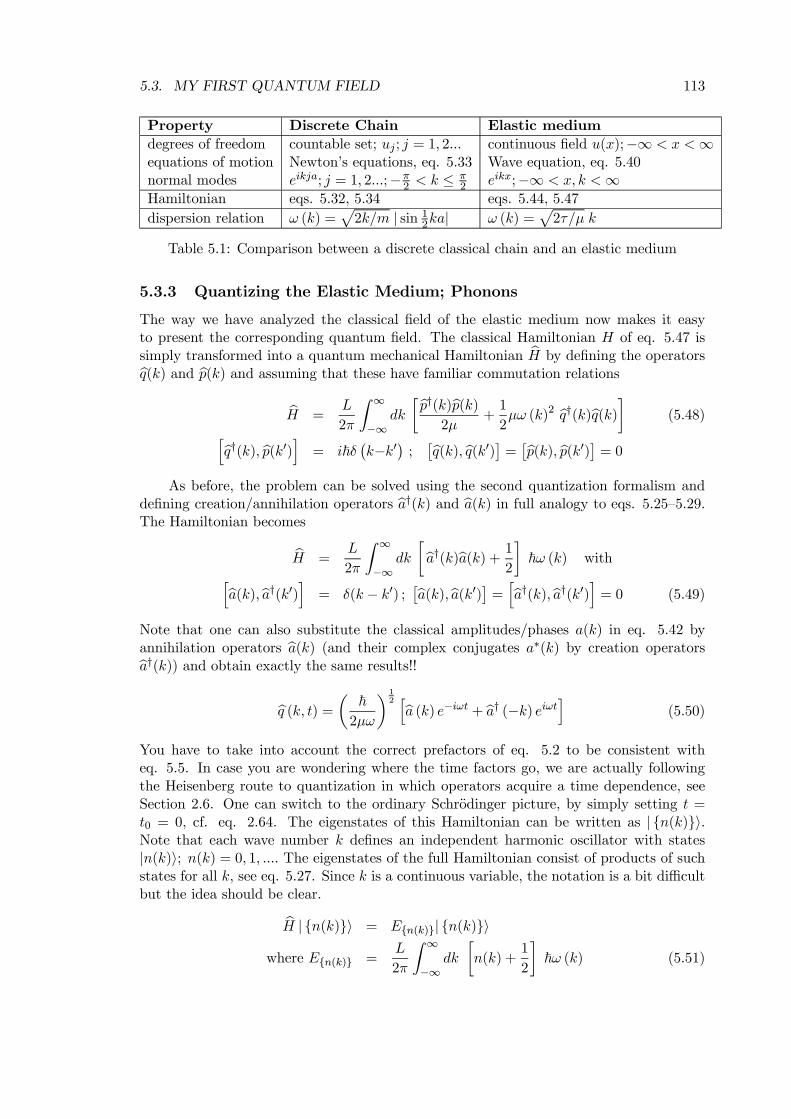
5.3. MY FIRST QUANTUM FIELD 113
Property Discrete Chain Elastic medium
degrees of freedom countable set; uj ; j = 1, 2... continuous field u(x);−∞ < x <∞equations of motion Newton’s equations, eq. 5.33 Wave equation, eq. 5.40normal modes eikja; j = 1, 2...;−π
2 < k ≤ π2 eikx;−∞ < x, k <∞
Hamiltonian eqs. 5.32, 5.34 eqs. 5.44, 5.47
dispersion relation ω (k) =p2k/m | sin 12ka| ω (k) =
p2τ/µ k
Table 5.1: Comparison between a discrete classical chain and an elastic medium
5.3.3 Quantizing the Elastic Medium; Phonons
The way we have analyzed the classical field of the elastic medium now makes it easyto present the corresponding quantum field. The classical Hamiltonian H of eq. 5.47 issimply transformed into a quantum mechanical Hamiltonian bH by defining the operatorsbq(k) and bp(k) and assuming that these have familiar commutation relations
bH =L
2π
Z ∞
−∞dk
·bp†(k)bp(k)2µ
+1
2µω (k)2 bq†(k)bq(k)¸ (5.48)hbq†(k), bp(k0)i = i~δ
¡k−k0¢ ; £bq(k), bq(k0)¤ = £bp(k), bp(k0)¤ = 0
As before, the problem can be solved using the second quantization formalism anddefining creation/annihilation operators ba†(k) and ba(k) in full analogy to eqs. 5.25—5.29.The Hamiltonian becomes
bH =L
2π
Z ∞
−∞dk
·ba†(k)ba(k) + 12
¸~ω (k) withhba(k),ba†(k0)i = δ(k − k0) ; £ba(k),ba(k0)¤ = hba†(k),ba†(k0)i = 0 (5.49)
Note that one can also substitute the classical amplitudes/phases a(k) in eq. 5.42 byannihilation operators ba(k) (and their complex conjugates a∗(k) by creation operatorsba†(k)) and obtain exactly the same results!!
bq (k, t) = µ ~2µω
¶ 12 hba (k) e−iωt + ba† (−k) eiωti (5.50)
You have to take into account the correct prefactors of eq. 5.2 to be consistent witheq. 5.5. In case you are wondering where the time factors go, we are actually followingthe Heisenberg route to quantization in which operators acquire a time dependence, seeSection 2.6. One can switch to the ordinary Schrodinger picture, by simply setting t =t0 = 0, cf. eq. 2.64. The eigenstates of this Hamiltonian can be written as | n(k)i.Note that each wave number k defines an independent harmonic oscillator with states|n(k)i; n(k) = 0, 1, .... The eigenstates of the full Hamiltonian consist of products of suchstates for all k, see eq. 5.27. Since k is a continuous variable, the notation is a bit difficultbut the idea should be clear.
bH | n(k)i = En(k)| n(k)i
where En(k) =L
2π
Z ∞
−∞dk
·n(k) +
1
2
¸~ω (k) (5.51)
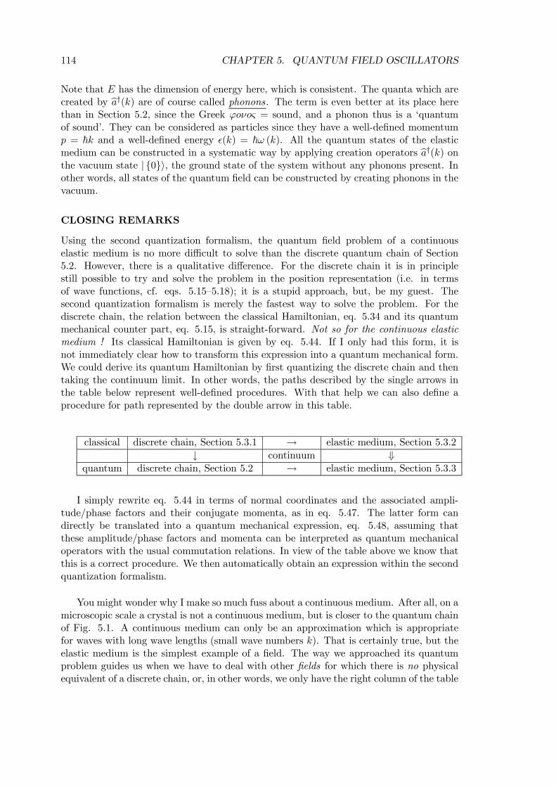
114 CHAPTER 5. QUANTUM FIELD OSCILLATORS
Note that E has the dimension of energy here, which is consistent. The quanta which arecreated by ba†(k) are of course called phonons. The term is even better at its place herethan in Section 5.2, since the Greek ϕoνoς = sound, and a phonon thus is a ‘quantumof sound’. They can be considered as particles since they have a well-defined momentump = ~k and a well-defined energy ²(k) = ~ω (k). All the quantum states of the elasticmedium can be constructed in a systematic way by applying creation operators ba†(k) onthe vacuum state | 0i, the ground state of the system without any phonons present. Inother words, all states of the quantum field can be constructed by creating phonons in thevacuum.
CLOSING REMARKS
Using the second quantization formalism, the quantum field problem of a continuouselastic medium is no more difficult to solve than the discrete quantum chain of Section5.2. However, there is a qualitative difference. For the discrete chain it is in principlestill possible to try and solve the problem in the position representation (i.e. in termsof wave functions, cf. eqs. 5.15—5.18); it is a stupid approach, but, be my guest. Thesecond quantization formalism is merely the fastest way to solve the problem. For thediscrete chain, the relation between the classical Hamiltonian, eq. 5.34 and its quantummechanical counter part, eq. 5.15, is straight-forward. Not so for the continuous elasticmedium ! Its classical Hamiltonian is given by eq. 5.44. If I only had this form, it isnot immediately clear how to transform this expression into a quantum mechanical form.We could derive its quantum Hamiltonian by first quantizing the discrete chain and thentaking the continuum limit. In other words, the paths described by the single arrows inthe table below represent well-defined procedures. With that help we can also define aprocedure for path represented by the double arrow in this table.
classical discrete chain, Section 5.3.1 → elastic medium, Section 5.3.2
↓ continuum ⇓quantum discrete chain, Section 5.2 → elastic medium, Section 5.3.3
I simply rewrite eq. 5.44 in terms of normal coordinates and the associated ampli-tude/phase factors and their conjugate momenta, as in eq. 5.47. The latter form candirectly be translated into a quantum mechanical expression, eq. 5.48, assuming thatthese amplitude/phase factors and momenta can be interpreted as quantum mechanicaloperators with the usual commutation relations. In view of the table above we know thatthis is a correct procedure. We then automatically obtain an expression within the secondquantization formalism.
You might wonder why I make so much fuss about a continuous medium. After all, on amicroscopic scale a crystal is not a continuous medium, but is closer to the quantum chainof Fig. 5.1. A continuous medium can only be an approximation which is appropriatefor waves with long wave lengths (small wave numbers k). That is certainly true, but theelastic medium is the simplest example of a field. The way we approached its quantumproblem guides us when we have to deal with other fields for which there is no physicalequivalent of a discrete chain, or, in other words, we only have the right column of the table
5.4. THE THREE-DIMENSIONAL QUANTUM CHAIN 115
above. A non-trivial example of the latter will be given in the final section of this chapter,namely the quantization of the electro-magnetic field, or quantum electrodynamics.9 Forsuch fields the second quantization formalism is not merely the fastest way to approach thecorresponding quantum field problem, it is the only way ! For such quantum fields it is nolonger possible to define a “position” representation; the occupation number representationis all we have got.
5.4 The Three-dimensional Quantum Chain
5.4.1 Discrete Lattice
The previous two Sections 5.2 and 5.3 have been concerned with one-dimensional problems.It is tedious, but not difficult in principle to extend the discussion to the three-dimensionalcase. The 3-dim chain is a good model to describe phonons in a simple crystal with oneatom per unit cell.10 Instead of the expression given in eq. 5.19, one obtains similarthree-dimensional expressions
bpk,s =1√N
XR
e−ik·R εk,s · bpRbqk,s =
1√N
XR
e−ik·R εk,s · buR (5.52)
It is assumed that the masses form a three-dimensional lattice, where R =la+mb+nc;l,m, n = 0, 1... are the lattice vectors describing the positions of the atoms in equilibrium.The atoms interact with their neighbors via harmonic potentials (the “springs”; if thedisplacements from equilibrium are small enough we may always approximate the fullpotential by an harmonic potential). uR = (ux, uy, uz)R is the displacement vector ofthe atom at the lattice position R; pR = (px, py, pz)R is its corresponding momentum. kis a vector in reciprocal space belonging to the first Brillouin zone. The vectors εk,s =(εx, εy, εz)k,s; s = 1, 2, 3; |εk,s|2 = 1 are called the polarization vectors. In a cubiccrystal, there is one longitudinal mode εk,1kk and two transversal modes εk,2, εk,3⊥k (and εk,2⊥εk,3). In an anisotropic crystal, the relation between the direction of k of thewave and the polarization vectors can be quite complicated.
Eq. 5.24 is replaced by
bH =Xk,s
bp†k,sbpk,s2m
+1
2mωs (k)
2 bq†k,sbqk,s (5.53)
9A general method to quantize classical fields exists, not based upon normal modes. The first step isto formulate a “classical mechanics” for fields within the Lagrangian formalism. A Hamiltonian is thendefined in the usual way via canonical momenta and coordinates. This is then quantized by turning thelatter into operators, assuming the usual commutation relations. This, in a nutshell is “quantum fieldtheory”. Useful references are: H. Goldstein, Classical Mechanics, (Addison-Wesley, Reading, 1980); forclassical fields, and W. Greiner, J. Reinhardt, Field Quantization (Springer, Berlin, 1996) for quantumfields.10The case of multiple atoms per unit cell is not much more difficult to treat, but there the notation
becomes really messy. If you want to know more about it, you should consult solid state physics books. Agood reference is: N. W. Ashcroft and N. D. Mermin, Solid State Physics, (Holt-Saunders, Philadelphia,1976).
116 CHAPTER 5. QUANTUM FIELD OSCILLATORS
where the sum over k covers the first Brillouin zone and s = 1, 2, 3 sums over the polariza-tions. The dispersion relations ωs (k) can be calculated straight-forwardly, once the lattice(fcc, bcc, hcp, etcetera all give different dispersion relations) and the interaction potentialbetween the atoms (the “spring” constants) are known.11 From here on we can switch tosecond quantization language and simply copy all the steps after eq. 5.24 to obtain thephonons of the three-dimensional lattice. The Hamiltonian is rewritten as
bH =Xk,s
µ1
2+ ba†k,sbak,s¶~ωs (k) withhbak,s,ba†k0,s0i = δk,k0 δs,s0 ;£bak,s,bak0,s0¤ = hba†k,s,ba†k0,s0i = 0 (5.54)
The eigenstates |nk,si can be constructed systematically by operating with the creationoperators ba†k,s on the vacuum state |0i. The operator ba†k,s creates a phonon with polar-ization s, momentum p =~k, and energy ²s (k) = ~ωs (k).
5.4.2 Elastic Medium
As in Section 5.3 we can take the continuum limit to describe (quantized) sound wavesin an elastic medium. A homogeneous and isotropic medium can be characterized by aspeed of sound for longitudinal and transversal waves vl, vt, respectively. The classicalwave equations in three dimensions, equivalent to eq. 5.40 are
∂2us(r, t)
∂t2= v2s∇2us(r, t) (5.55)
where the subscript s indicates longitudinal or transversal. The total displacement fieldPs us(r, t) ≡ u(r, t) = (ux(r, t), uy(r, t), uz(r, t)) is a three dimensional vector, where each
component depends upon the position in space r =(x, y, z) and time t. The transition toquantum mechanics follows exactly the procedure outlined in Section 5.3 in one dimension,where we assign different polarization directions to the one longitudinal and two transversalmodes, as for the isotropic (cubic) crystal. So the equivalent of eq. 5.41 in three dimensionsbecomes
u(r, t) =
√Ω
(2π)3
Xs
Z ∞
−∞eik·rεk,sqs(k, t)d3k (5.56)
with ωs(k) = vsk, as before. The normalization constant is the three-dimensional analogueof eq. 5.45, where Ω = L3 is some convenient normalization volume. The spatial dependentfunctions εk,se
ik·r labeled by s = 1, 2, 3 and k are again called the modes of the system.Per k there is one longitudinal mode εk,1kk and two transversal modes εk,2, εk,3⊥k ( andεk,2⊥εk,3) with speeds vl, vt, respectively.12 The quantum mechanical operators bqs(k) andbps(k) equivalent to eq. 5.52 can be written as
bps(k) =1√Ω
Z ∞
−∞e−ik·r εk,s · bp(r) d3r
bqs(k) =1√Ω
Z ∞
−∞e−ik·r εk,s · bu(r) d3r (5.57)
11See Ashcroft & Mermin.12This is only true in an isotropic medium. In an anisotropic medium polarizations become much more
complicated. Also the speed of sound is different for different directions in the medium.
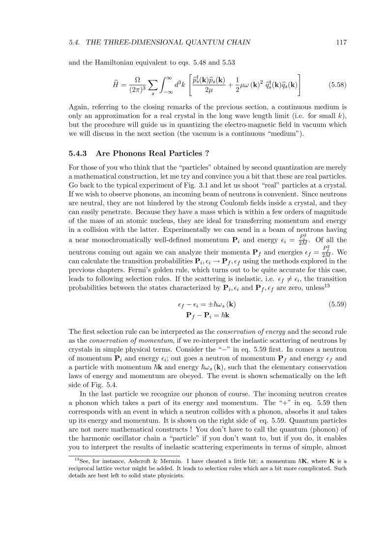
5.4. THE THREE-DIMENSIONAL QUANTUM CHAIN 117
and the Hamiltonian equivalent to eqs. 5.48 and 5.53
bH =Ω
(2π)3
Xs
Z ∞
−∞d3k
"bp†s(k)bps(k)2µ
+1
2µω (k)2 bq†s(k)bqs(k)
#(5.58)
Again, referring to the closing remarks of the previous section, a continuous medium isonly an approximation for a real crystal in the long wave length limit (i.e. for small k),but the procedure will guide us in quantizing the electro-magnetic field in vacuum whichwe will discuss in the next section (the vacuum is a continuous “medium”).
5.4.3 Are Phonons Real Particles ?
For those of you who think that the “particles” obtained by second quantization are merelya mathematical construction, let me try and convince you a bit that these are real particles.Go back to the typical experiment of Fig. 3.1 and let us shoot “real” particles at a crystal.If we wish to observe phonons, an incoming beam of neutrons is convenient. Since neutronsare neutral, they are not hindered by the strong Coulomb fields inside a crystal, and theycan easily penetrate. Because they have a mass which is within a few orders of magnitudeof the mass of an atomic nucleus, they are ideal for transferring momentum and energyin a collision with the latter. Experimentally we can send in a beam of neutrons having
a near monochromatically well-defined momentum Pi and energy ²i =P 2i2M . Of all the
neutrons coming out again we can analyze their momenta Pf and energies ²f =P 2f2M . We
can calculate the transition probabilities Pi, ²i → Pf , ²f using the methods explored in theprevious chapters. Fermi’s golden rule, which turns out to be quite accurate for this case,leads to following selection rules. If the scattering is inelastic, i.e. ²f 6= ²i, the transitionprobabilities between the states characterized by Pi, ²i and Pf , ²f are zero, unless
13
²f − ²i = ±~ωs (k) (5.59)
Pf −Pi = ~k
The first selection rule can be interpreted as the conservation of energy and the second ruleas the conservation of momentum, if we re-interpret the inelastic scattering of neutrons bycrystals in simple physical terms. Consider the “−” in eq. 5.59 first. In comes a neutronof momentum Pi and energy ²i; out goes a neutron of momentum Pf and energy ²f anda particle with momentum ~k and energy ~ωs (k), such that the elementary conservationlaws of energy and momentum are obeyed. The event is shown schematically on the leftside of Fig. 5.4.
In the last particle we recognize our phonon of course. The incoming neutron createsa phonon which takes a part of its energy and momentum. The “+” in eq. 5.59 thencorresponds with an event in which a neutron collides with a phonon, absorbs it and takesup its energy and momentum. It is shown on the right side of eq. 5.59. Quantum particlesare not mere mathematical constructs ! You don’t have to call the quantum (phonon) ofthe harmonic oscillator chain a “particle” if you don’t want to, but if you do, it enablesyou to interpret the results of inelastic scattering experiments in terms of simple, almost
13See, for instance, Ashcroft & Mermin. I have cheated a little bit; a momentum ~K, where K is areciprocal lattice vector might be added. It leads to selection rules which are a bit more complicated. Suchdetails are best left to solid state physicists.
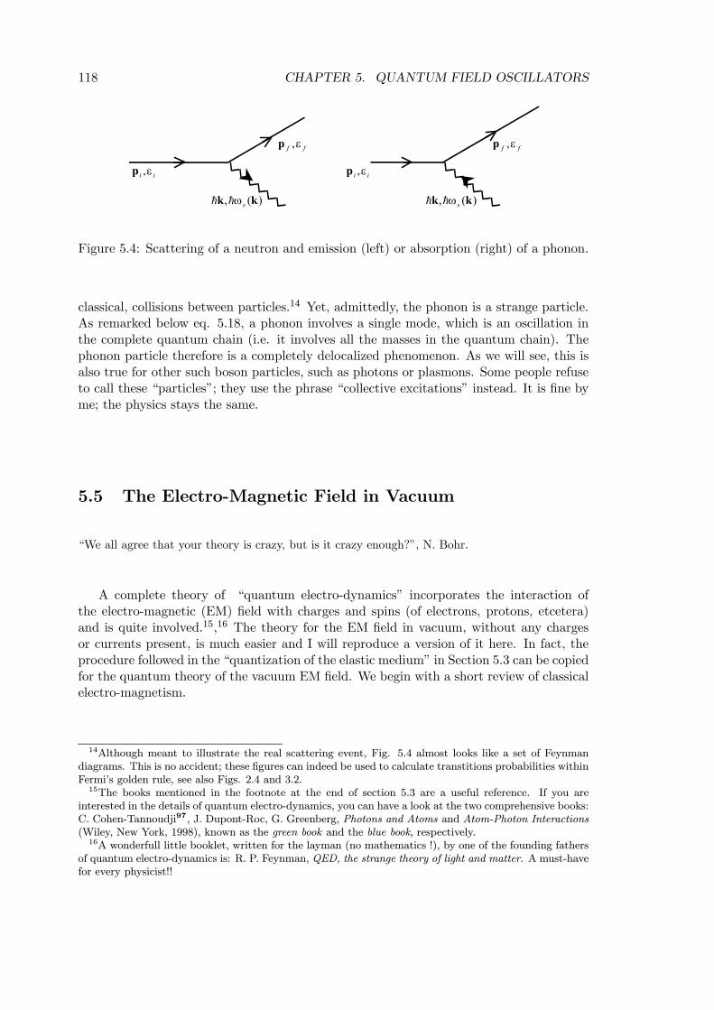
118 CHAPTER 5. QUANTUM FIELD OSCILLATORS
ii ε,p
)(, kk sω
ff ε,p
ii ε,p
)(, kk sω
ff ε,p
Figure 5.4: Scattering of a neutron and emission (left) or absorption (right) of a phonon.
classical, collisions between particles.14 Yet, admittedly, the phonon is a strange particle.As remarked below eq. 5.18, a phonon involves a single mode, which is an oscillation inthe complete quantum chain (i.e. it involves all the masses in the quantum chain). Thephonon particle therefore is a completely delocalized phenomenon. As we will see, this isalso true for other such boson particles, such as photons or plasmons. Some people refuseto call these “particles”; they use the phrase “collective excitations” instead. It is fine byme; the physics stays the same.
5.5 The Electro-Magnetic Field in Vacuum
“We all agree that your theory is crazy, but is it crazy enough?”, N. Bohr.
A complete theory of “quantum electro-dynamics” incorporates the interaction ofthe electro-magnetic (EM) field with charges and spins (of electrons, protons, etcetera)and is quite involved.15,16 The theory for the EM field in vacuum, without any chargesor currents present, is much easier and I will reproduce a version of it here. In fact, theprocedure followed in the “quantization of the elastic medium” in Section 5.3 can be copiedfor the quantum theory of the vacuum EM field. We begin with a short review of classicalelectro-magnetism.
14Although meant to illustrate the real scattering event, Fig. 5.4 almost looks like a set of Feynmandiagrams. This is no accident; these figures can indeed be used to calculate transtitions probabilities withinFermi’s golden rule, see also Figs. 2.4 and 3.2.15The books mentioned in the footnote at the end of section 5.3 are a useful reference. If you are
interested in the details of quantum electro-dynamics, you can have a look at the two comprehensive books:C. Cohen-Tannoudji97, J. Dupont-Roc, G. Greenberg, Photons and Atoms and Atom-Photon Interactions(Wiley, New York, 1998), known as the green book and the blue book, respectively.16A wonderfull little booklet, written for the layman (no mathematics !), by one of the founding fathers
of quantum electro-dynamics is: R. P. Feynman, QED, the strange theory of light and matter. A must-havefor every physicist!!
5.5. THE ELECTRO-MAGNETIC FIELD IN VACUUM 119
5.5.1 Classical Electro-Dynamics
The classical electro-magnetic field is given by Maxwell’s equations, which in vacuum (nocharges or currents present) read17
∇×E = −∂B∂t
∇ ·E = 0
∇×B = ε0µ0∂E
∂t∇ ·B = 0 (5.60)
Calculating∇×∇×E and∇×∇×B , using∇×∇× a =∇(∇ · a)−∇2a and∇ · a =0 for a = E,B, and using ε0µ0 =
1c2, we get
∇2E = 1c2∂2E
∂t2and ∇2B = 1
c2∂B2
∂t2(5.61)
Both the electric field E (r, t) and the magnetic field B(r, t) are solutions of a wave equa-tion. Note the resemblance with eq. 5.55. The general solutions of these wave equationseq. 5.61 can then be written as in analogy with eq. 5.56
E (r, t) =
√Ω
(2π)3
Zd3k E (k, t) eik·r
B (r,t) =
√Ω
(2π)3
Zd3k B (k, t) eik·r (5.62)
where again Ω is some convenient normalization volume. Assuming that these fields canbe represented by real numbers one has the general form
E (k, t) = E0 (k) e−iωt +E∗0 (−k) eiωt
B (k, t) = B0 (k) e−iωt +B∗0 (−k) eiωt (5.63)
You can check it explicitly that eqs. 5.62 and 5.63 constitute a solution of eq. 5.61 if thefollowing holds
ω = ck (5.64)
(k = |k|), which is the familiar dispersion relation for EM waves in vacuum. Again note theresemblance with eq. 5.56. Apparently, the general solution of the EM field in vacuumcan be written as a linear combination of modes eik·r. The coefficients E0 (k) , B0 (k)can in principle be completely arbitrary but Maxwell’s equations, eq. 5.60, place somerestrictions. Using eq. 5.62 in eq. 5.60, the div’s lead to
k ·E0(k) = 0 k ·B0 (k) = 0
whereas the rot’s give
k×E0(k) = ωB0(k) k×B0(k) = −ωε0µ0E0(k)17In SI (rationalized mks) units. For a discussion on the various systems of units, see the appendix in W.
K. H. Panofsky and M. Phillips, Classical Electricity and Magnetism, (Addison-Wesley, Reading, 1978).
120 CHAPTER 5. QUANTUM FIELD OSCILLATORS
Or in other words
E0 (k) ⊥ B0 (k) ⊥ k and |E0 (k)| = c |B0 (k)| (5.65)
The wave vector k denotes the direction of propagation of the plane wave eik·r. Maxwell’sequations show that in vacuum EM waves are transversal, i.e. both electric and magneticfields are perpendicular to the direction of propagation, and the amplitudes and phases ofthe latter are coupled. We can define two polarization vectors εk,1, εk,2⊥k and εk,1⊥εk,2,and write
E (r, t) =
√Ω
(2π)3
Xs=1,2
Zd3k Es (k, t) εk,se
ik·r (5.66)
where Es (k, t) denotes the amplitudes and phases, which classically can have any contin-uous value. The functions εk,se
ik·r are again called the modes of the system; they canbe labeled with the wave vector k and polarization s. The general solutions of the waveequation can be written as a linear combination of the modes. The magnetic field can beobtained using the relations given in eq. 5.65.
If we are not in free space, but in a cavity or wave guide, for instance, the modes canhave a much more complicated form than just simple plane waves. This depends uponthe boundary conditions on the walls of the wave guide or cavity.18 Whatever the shapeof the wave guide or cavity, one can always obtain a set of modes fk1k2k3s(r) which arelabeled by three numbers, k1, k2,k3 and a polarization s = 1, 2. One can always write theelectric field as a linear combination of these modes.
E (r, t) =
√Ω
(2π)3
Zdk1dk2dk3Es (k1k2k3; t) fk1k2k3s (r) (5.67)
In a closed cavity, the index ki is not continuous, but discrete (remember a particle ina box); in that case we simply replace the integral by a sum over the discrete indexRdki →
Pkias usual. The magnetic field can be obtained from the electric field by
relations similar (but not identical !!) to eq. 5.65. The time dependence is set by the waveequation, eq. 5.61.
It is well known from classical EM theory that instead of working with E and B fieldsplus the restrictions of eq. 5.65 which are dictated by Maxwell’s equations, it is convenientto work with potentials. As usual we choose a vector potential A (r, t) with ∇ ·A = 0
(the so-called Coulomb gauge), such that
B =∇×A
From Maxwell’s equations one then shows that
E = −∂A∂t
18If a wall is an ideal conductor, the electric field should be perpendicular to the wall, etcetera; youknow this stuff from your electricity & magnetism courses.
5.5. THE ELECTRO-MAGNETIC FIELD IN VACUUM 121
Note that the scalar potential φ (r,t) = 0 in the absence of charges. By choosing thisvector potential we automatically obey the two equations ∇ ·B = 0 and ∇ ·E = 0. Thetwo other Maxwell’s equations can then be combined to the wave equation
∇2A =1
c2∂2A
∂t2(5.68)
with the obvious general solution
A (r, t) =
√Ω
(2π)3
Xs=1,2
Zd3k As (k, t) εk,se
ik·r (5.69)
Because ∇ ·A = 0, it follows k · ²ks = 0; s = 1, 2; we have the familiar two transversalwaves. Because A (r, t) has to be real and a solution of eq. 5.68, the numbers As (k, t)have the general form
As (k, t) = as (k) e−iωt + a∗s (−k) eiωt (5.70)
with ω = ck, as before. Again note the resemblance with eqs. 5.55 and 5.56. One caneasily check that the relations of eq. 5.65 are automatically fulfilled. The vector potentialthis is the easiest way to set up EM theory; everything else can be derived from it.
5.5.2 Quantum Electro-Dynamics (QED)
Classically, eqs. 5.69, 5.70 solve the EM problem in vacuum. From the foregoing I guessthat by now you got the idea of how this is quantized. The vacuum is not a mediumin the sense of Sections 5.3 and 5.4; we have no “quantum chain” to start from.19 Thismeans that we cannot start from a Schrodinger equation of a quantum chain. Quantumis more complex and more detailed than classical. We can go from quantum to classicalmechanics by making well-defined approximations. Going the other way, from classical toquantum mechanics, one has to guess what these approximations could look like. There isno systematic way for doing this. Schrodinger and Heisenberg were independently inspiredby classical mechanics, made an educated guess for quantum mechanics, and arrived at theSchrodinger and Heisenberg equations, respectively. For a classical field which is not basedupon classical mechanical particles, like the EM field, we must use a different guess. Oneoption is to first devise a version of “classical mechanics” which can describe fields; see thefootnote at the end of Section 5.3. That route is very general, but also very formal. Wetake a short-cut here. In Sections 5.3 and 5.4 we quantized the elastic medium, which canbe based upon mechanical particles (the “quantum chain”), in a way which was consistentwith the Schrodinger equation for the particles in the quantum chain. Inspired by this,we close our eyes, and follow the same recipe for the EM field. So comparing eq. 5.69 toeq. 5.56 we know what gets quantized: the numbers As (k, t) become operators bqs (k, t).In quantum mechanics the vector potential becomes an operator.
bA (r, t) = √Ω
(2π)3
Xs=1,2
Zd3k bqs (k, t) εk,seik·r (5.71)
19In the 19th century EM waves were thought to propagate in a sort of elastic medium called the “aether”.Already Maxwell hadn’t much use for it; his equations work fine without it. After Einstein’s theory ofrelativity, it became completely obsolete.
122 CHAPTER 5. QUANTUM FIELD OSCILLATORS
where
bqs (k, t) = µ ~2ε0ω
¶12 hbas (k) e−iωt + ba†s (−k) eiωti (5.72)
Compare 5.70 to eqs. 5.38 and 5.50. Again the time dependence emerges because we followthe “Heisenberg route” to quantization, i.e. we start from the classical time dependent“observable” and directly quantize it into an operator, as explained in Section 2.6. Theconnection to the usual “Schrodinger picture”, where the operators are time-independent(and instead the states are time-dependent), can be made by simply setting t = t0 = 0in the equations above, cf. eq. 2.64. The basic idea of quantizing the EM field is that,like in the elastic medium case, we want the intensity of the EM field to be proportionalto the number of photons (so much we know from experiment), so we must quantize theamplitudes in order to achieve this.
IMPORTANT MESSAGE
The classical modes εk,seik·r are not changed, so these are not quantum wave functions.
Don’t make the mistake of calling εk,seik·r the “wave function of the photon in vacuum”.
It is not ; it simply is the classical mode. It is the amplitude which gets quantized, notthe mode. Compare to the discrete quantum chain. The modes are defined by eq. 5.37;the wave function for the particles in the chain is given by eq. 5.18; these are completelydifferent things !! In a wave guide or cavity, which has classical modes fk1k2k3s(r), thequantum equivalent of eq. 5.66 for the vector potential becomes
bA (r, t) = √Ω
(2π)3
Zdk1dk2dk bqs (k1k2k3, t) fk1k2k3s (r)
which stresses again that the amplitudes, not the modes, are quantized . The position r is
simply a continuous index for the bA operator, likeR was a discrete (lattice) position indexin the quantum chain of eq. 5.52. Again, do not get confused with wave functions; ther-dependence has nothing to do with that.
The classical E and B fields can be derived from eq. 5.69
B (r, t) = ∇×A =i√Ω
(2π)3
XZd3k eik·r (k× εk,s) qs (k,t)
E (r, t) = −∂A∂t
= −√Ω
(2π)3
Xs
Zd3k eik·r εk,sqs (k,t) (5.73)
The transition to quantummechanics can be completed by defining a conjugate momentumanalogous to eq. 5.46
ps (k,t) = ²0qs (k,t) (5.74)
and making the p0s and q0s quantum operators
bB (r, t) → bqs (k,t)bE (r,t) → bps (k,t) (5.75)
5.5. THE ELECTRO-MAGNETIC FIELD IN VACUUM 123
Note that the E and B fields become operators bE and bB. Such operators which dependupon a continuous index (r) are called quantum fields. We assume that the q’s and p’shave familiar commutation relationshbq†s(k), bps0(k0)i = i~δ
¡k− k0¢ δss0 and£bqs(k), bqs0(k0)¤ =
£bps(k), bps0(k0)¤ = 0 (5.76)
where we have set t = 0 in order to obtain operators in the “Schrodinger picture”. Havingdefined the relevant operators, how do we find the quantum “states” of the EM field? Asin Section 5.46 we do this by starting from the classical energy. The energy of a classicalEM field in a volume Ω is given by
H =
Zd3r
1
2
·ε0 |E (r, t)|2 + 1
µ0|B (r, t)|2
¸(5.77)
We quantize by identifying this classical energy with the quantum mechanical HamiltonianbH. Using eqs. 5.73—5.77, the relations ε0µ0 = 1c2and ω = kc we find
bH =Ω
(2π)3
Xs
Zd3k
"bp†s(k)bps(k)2ε0
+1
2ε0ω
2bq†s(k)bqs(k)#
(5.78)
This looks like the familiar sum of harmonic oscillators again, see e.g. 5.48 and by nowwe know how to solve this. Write
bH =Ω
(2π)3
Xs
Zd3k
½1
2+ ba†s(k)bas(k)¾ ~ωhbas(k),ba†s0(k0)i = δ
¡k− k0¢ δss0 andhba†s(k),ba†s0(k0)i = £bas(k),bas0(k0)¤ = 0 (5.79)
in terms of creation and annihilation operators, where
bas(k) = ³ε0ω2~
´ 12 bqs(k) + iµ 1
2~ε0ω
¶ 12 bps(k)
Note that these relations are consistent with eq. 5.72. The eigenstates of this Hamiltonianare given by
| ns(k)i =Yks
|ns(k)i = |n1(k1)i|n2(k1)i|n1(k2)i|n2(k2)i....|n1(ki)i|n2(ki)i...
Each state |ns(ki)i contains a number of ns(ki) quanta in mode ki and polarization s.Each quantum has an energy ~ω = ~cki and a momentum ~ki. All the quanta belongingto one mode ki and polarization s are indistinguishable and we can put as many intoeach mode as we want. They can be considered as particles and are called photons, afterthe Greek ϕoτoς which means “light”. A “photon” thus is a “light particle”. Obviously,photons are bosons.
124 CHAPTER 5. QUANTUM FIELD OSCILLATORS
CLOSING REMARKS
• We have derived the quantum form of the vacuum EM field by analogy with theelastic medium for phonons. You cannot prove a priori that this is the correct way toquantize the classical (Maxwell) equations. But then again you also cannot “prove”the Schrodinger wave equation starting from classical mechanics for particles. Youhave to postulate that this is the correct form and find out whether this predicts theright results for experiments (it does).
• The quantum chain and the vacuum EM field were examples in which the particles(phonons or photons) do not interact with each other, i.e. they are independent par-ticles. If we introduce interaction terms, things get more complicated. For instance,anharmonic interactions in the quantum chain of a type bxnbxmbxl, or non-linear termsin the EM field, which are caused by interactions with matter. Such interactionterms can play the role of a perturbation bV , for which we developed time-dependentperturbation theory or the Green function techniques in the previous chapters.
• Another type of interaction is letting the bosons (photons/phonons) interact withor decay into fermions. For instance, when a photon is absorbed in a crystal, thephoton (boson) is annihilated while at the same time an electron and a hole (twofermions) are created. The photon energy is then usually on the scale of 1 eV . Inhigh energy physics a similar process can happen on a slightly higher energy scale.A γ-photon with an energy ∼ 106 eV is annihilated and an electron and a positronare created. By analogy, the latter is a hole in the vacuum. Again such interactionscan play the role of a perturbation bV .
5.5.3 Are Photons Real Particles ?
This same questions we had with phonons arise again and I can use the same argumentsto try and convince you that photons are particles. Here I have a little bit more to startfrom. We limit our discussion to a single mode A (r) = qs(k) εk,se
ik·r. First we provethat the photon momentum is given by p =~k. A classical EM field possesses momentumas well as energy. Using Maxwell’s equations one can prove that the momentum of an EMwave is given by (using Poynting’s theorem)
p = ε0
Zd3r E×B
It is perpendicular both to E, the electric, andB the magnetic field and thus, in view of eq.5.65, it is in the direction of propagation of the wave k. Since E and B are perpendicularas well, its size is
|p| = ε0|E||B| =ε0c|E|2 = ε0c|B|2 =
=1
2c
½ε0|E|2 + 1
µ0|B|2
¾=1
cH
using eq. 5.77. In other words, the classical momentum is given by
p =H
c
k
k=H
ωk
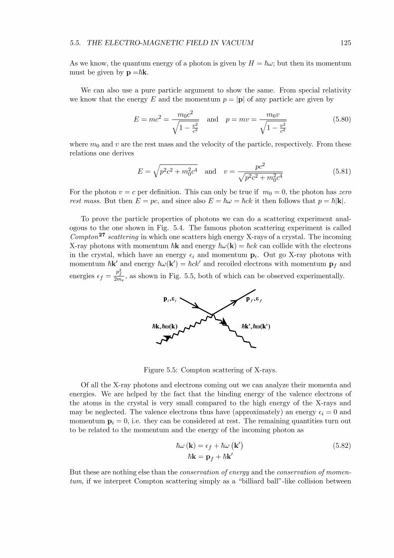
5.5. THE ELECTRO-MAGNETIC FIELD IN VACUUM 125
As we know, the quantum energy of a photon is given by H = ~ω; but then its momentummust be given by p =~k.
We can also use a pure particle argument to show the same. From special relativitywe know that the energy E and the momentum p = |p| of any particle are given by
E = mc2 =m0c
2q1− v2
c2
and p = mv =m0vq1− v2
c2
(5.80)
where m0 and v are the rest mass and the velocity of the particle, respectively. From theserelations one derives
E =qp2c2 +m2
0c4 and v =
pc2pp2c2 +m2
0c4
(5.81)
For the photon v = c per definition. This can only be true if m0 = 0, the photon has zerorest mass. But then E = pc, and since also E = ~ω = ~ck it then follows that p = ~|k|.
To prove the particle properties of photons we can do a scattering experiment anal-ogous to the one shown in Fig. 5.4. The famous photon scattering experiment is calledCompton27 scattering in which one scatters high energy X-rays of a crystal. The incomingX-ray photons with momentum ~k and energy ~ω(k) = ~ck can collide with the electronsin the crystal, which have an energy ²i and momentum pi. Out go X-ray photons withmomentum ~k0 and energy ~ω(k0) = ~ck0 and recoiled electrons with momentum pf and
energies ²f =p2f2me
, as shown in Fig. 5.5, both of which can be observed experimentally.
)'(,' kk ω
ff ε,p
)(, kk ω
ii ε,p
)'(,' kk ω
ff ε,p
)(, kk ω
ii ε,p
Figure 5.5: Compton scattering of X-rays.
Of all the X-ray photons and electrons coming out we can analyze their momenta andenergies. We are helped by the fact that the binding energy of the valence electrons ofthe atoms in the crystal is very small compared to the high energy of the X-rays andmay be neglected. The valence electrons thus have (approximately) an energy ²i = 0 andmomentum pi = 0, i.e. they can be considered at rest. The remaining quantities turn outto be related to the momentum and the energy of the incoming photon as
~ω (k) = ²f + ~ω¡k0¢
(5.82)
~k = pf + ~k0
But these are nothing else than the conservation of energy and the conservation of momen-tum, if we interpret Compton scattering simply as a “billiard ball”-like collision between
126 CHAPTER 5. QUANTUM FIELD OSCILLATORS
a photon and an electron particle. The conservation rules of eq. 5.82 can be derived asselection rules, using the by now familiar perturbation theory. Compton’s experiment wasvery important historically in convincing people of the particle properties of EM radia-tion, since it is extremely difficult, if not impossible, to explain the results by any othermeans.20
As we have seen in the case of phonons, photons are kind of strange particles. Eachphoton is created into a fixed mode with spatial dependence eik·r and polarization εk,swhich is just the classical mode (that is, in vacuum; in a wave guide/cavity, the mode is amore complicated fk1k2k3s (r)). Do not confuse this with a wave function in the quantummechanical sense; a photon has no wave function. The photon “exists” at all positionsin the mode and is completely delocalized. Think of the analogy to the quantum chain,where a single phonon is a quantum of a vibration which extends over the whole chain.Again, some people prefer to use the term “collective excitation” (in this case: of thevacuum). Photons are very fragile particles, they interact with any particle which hasa charge, such as electrons and protons. They also interact with any quasi-particle orcollective excitation which involves a charge distribution, such as phonons and plasmons.As a result of such interactions, photons are very easily created or annihilated and theirnumber is almost never constant or even very well-defined.
20If you want to know more about Compton scattering, have a look at S. Gasiorowicz, Quantum Physics(Wiley, New York, 1974), Ch.1; or B. H. Brandsen and C. J. Joachain, Quantum Mechanics (Prentice Hall,Harlow, 2000), Ch.1.
Chapter 6
Bosons and Fermions
“The creatures outside looked from pig to man, and from man to pig, and from pig to man again;
but already it was impossible to say which was which”, George Orwell, Animal Farm.
In the previous chapter we discussed many-boson systems that could entirely be de-scribed in terms of harmonic oscillators. We obtained an elegant simple picture by usinga special set of states and operators to set up the so-called occupation number represen-tation. In this chapter we extend this technique to make it more generally applicableto bosons, as well as fermions. In this case we start from a “traditional” wave functionrepresentation and work our way to the number representation. The latter is in fact moregeneral and also applies to systems like the EM field, where the former does not apply, aswe have seen in the previous chapter. At first the material will be a bit tedious, since manyparticle states involve a lot of book-keeping, I can’t help that. However, the final resultswill be again be very elegant and physical applications will follow. There is a good dis-cussion of many-fermion states in Mattuck’s book. Chapter 4, p. 64-72 (§ 4.1 - 4.3) givesa general introduction. Chapter 7, p. 123-141 gives a full picture. In this chapter I willstart from a single particle and then build in the wave-function-like way a many-particlestate (first quantization). Then I will introduce the occupation number representation, orsecond quantization technique, for bosons and fermions, respectively. Second quantization(for fermions here) allows for a reinterpretation of the results in terms of particles andanti-particles. I will also try and give some explanation for the seemingly strange name“second quantization” and give you some physical insight in particles and holes. AppendixI contains all the detailed algebra of occupation number representation and proofs of thestatements made in the text. For those of you who are interested in some background,Appendix II discusses why identical particles create a problem in quantum mechanics andwhat the way out is (the symmetry postulate). You might want to start by re-readingChapter 1, Section 1.4.
6.1 N particles; the Stone Age
Let φm (r1) be a wave function for a single particle, and the set of functions m = 1, 2, ....form a basis set. If we have a system of N of such particles (N ≥ 2), a basis set is formedby the product functions
φm1(r1) · φm2
(r2) · ........ · φmN(rN ) (6.1)
127
128 CHAPTER 6. BOSONS AND FERMIONS
where all the indices mi; i = 1, ......N independently can assume all allowed values, mi =1, 2, .... (see Section 1.4). In the following we will use Dirac notation and write |m (1)iinstead of φm (r), meaning that particle no. 1 is in a state |mi. In this notation, theproduct state of eq. 6.1 becomes
|m1 (1)i|m2 (2)i.......|mN (N)i ≡ |m1 (1)m2 (2) .......mN (N)i (6.2)
which means that particle 1 is in state |m1i, particle 2 is in state |m2i, ..., particle N isin state |mN i. The most general N -particle state can written as a linear combination ofsuch states.
|Ψ(1, 2, ..., N)i =Xm1
Xm2
...XmN
Cm1m2...mN|m1 (1)m2 (2) .......mN (N)i
with the coefficients Cm1m2...mN= hm1 (1)m2 (2) .......mN (N) |Ψ(1, 2, ..., N)i
Let us consider the single basis state of eq. 6.2. If the particles are identical, they shouldper definition be indistinguishable (Appendix II). However, writing down in which state weput each particle implies that we can distinguish the particles (particle 1 is in state |m1i,particle 2 is in state |m2i, etcetera), since these states can be different. We could use thestate numbers m1,m2, ... to label the particles. We could call the particle marked m1 the“blue” particle, the one called m2 the “red” particle, etcetera. In principle, m can labelthe eigenstates of an observable, so the “color” of the particle could be measured. Clearlywe have found a way to distinguish the particles, see also the discussion in Appendix II.Thus the state of eq. 6.2 is not entirely physical. We should in fact not be able to make adistinction with, for instance, a state in which particle 1 is in state |m2i and particle 2 isin state |m1i. To be specific, let bP12 be an operator which interchanges the two particles1 and 2.
bP12|m1 (1)m2 (2) ....mN (N)i = |m1 (2)m2 (1) .......mN (N)i
The only way (within a linear vector space) to ensure that we are not able to tell whichof the particles 1 or 2 occupies |m1i or |m2i, is to make a linear combination between thisstate and the one from eq. 6.2
|m1 (1)m2 (2) .......mN (N)i+ eiϕ|m1 (2)m2 (1) .......mN (N)i =(1 + eiϕ bP12)|m1 (1)m2 (2) .......mN (N)i
Both terms in this expression have an equal weight, but the coefficient’s phase ϕ we don’tknow a priori.1 Realizing that a similar thing must hold for any permutation bP in whichthe N particles are distributed/permutated over the states |m1i|m2i.....|mN i, it followsthat states that are allowed for indistinguishable particles, must be linear combinations inwhich all these permutated states appear with equal weightsX
bPeiϕp bP |m1 (1)m2 (2) .........mN (N)i
1The most general linear combination has a form like c1φ(1, 2)+ c2φ(2, 1), using an obvious short-handnotation. Since both terms must have equal weight, |c1| = |c2|. Writing c1 = |c1|eiϕ1 and c2 = |c2|eiϕ2 ,one can rewrite this linear combination in the form c1[φ(1, 2) + e
i(ϕ2−ϕ1)φ(2, 1)]. Setting c1 = 1 andϕ = ϕ2 − ϕ1 results in the form given.
6.1. N PARTICLES; THE STONE AGE 129
where bP is a permutation operating on the particles and the sum is over all N ! possiblepermutations, i.e. over all possible orderings of the N particles. A priori, it may seem thatwe cannot say anything about the phase factors eiϕp . However, a fundamental postulateof quantum mechanics, called the symmetry postulate, states that only two forms of N-particle states are actually allowed .2
The first special form is called the totally symmetric state, where all the phase factors
eiϕp = 1
|m1m2.......mN i(s) = NsXbPbP |m1 (1)m2 (2) .........mN (N)i (6.3)
where Ns is a normalization constant we will determine later on. It is straightforward toprove that if bPij is a permutation which interchanges particles i and j then
bPij |m1m2.....mNi(s) = |m1m2......mNi(s) (6.4)
See Appendix I for this proof. The idea is that, using the right hand side of eq. 6.3, ifbP runs over all possible N ! permutations, the product bPij bP also runs over all possibleN ! permutations. Since every permutation can be decomposed into a series of successiveinterchanges of two particles, if eq. 6.4 holds for any interchange bPij , it also holds for anyarbitrary permutation bP . The state |m1m2.......mNi(s) does not change if we permutatethe particles. We say that this state is symmetric with respect to all possible interchanges,or permutations of particles. In other words, we can no longer identity which particularparticle is in which state, which is what we wanted.
The second special form is called the totally anti-symmetric state and is written as
|m1m2....mNi(a) = NaXbP(−1)p bP |m1 (1)m2 (2) ....mN (N)i (6.5)
The phase factors are eiϕp = ±1 according to the following rule: the number (−1)p = 1,or p = 0, if the permutation bP can be written as an even number of interchanges and(−1)p = −1, or p = 1, if the permutation bP is equivalent to an odd number of interchanges.We have
bPij |m1m2.....mN i(a) = −|m1m2......mN i(a) (6.6)
See Appendix I. The idea is that each permutation bP in eq. 6.5 is even or odd, i.e.(−1)p = ±1; the single interchange bPij is odd per definition, i.e. (−1)pij = −1, so theproduct bPij bP is odd/even, i.e. (−1)p+pij = ∓1). We say that this state is anti-symmetricwith respect to all possible interchanges of particles. As always in quantum mechanics thestate |m1m2.....mN i(a) = |.....i(a) is not directly observable. What can be measured areexpectation values (a)h....| bA|....i(a), where bA is some (observable) operator. So minus signs(−) like in eq. 6.6 seem to have no influence on expectation values.
2This postulate should be added to the ones given in the first chapter. It is a true postulate; one canmake it plausible (see appendix II), but it cannot be proved from other physical postulates.
130 CHAPTER 6. BOSONS AND FERMIONS
One should however not draw the conclusion that the minus sign is unimportant. It hasvery important consequences, because it leads to the Pauli45 exclusion principle. This canbe derived as follows; suppose two of the numbers ml in eq. 6.6 are identical, for instancemi = mj . Then we have
bPij |...mi...mj ...i(a) = |...mj ...mi...i(a) = |...mi...mj ...i(a) (a)
since obviously a state cannot change if we interchange two identical numbers. On theother hand, because of eq. 6.6 we have
bPij |...mi...mj ...i(a) = −|...mi...mj ...i(a) (b)
By an elementary theorem of linear vector algebra, both (a) and (b) can only be truesimultaneously if |...mi...mj ...i(a) =|i the “null” vector of vector space. It follows that forany state |...mi...mj ...i(a) which is not the (trivial) null vector, all the numbers ml; l =1, .., N must be different from one another. Or, in other words, in the anti-symmetric stateall the particles must be in different one-particle states. If one particle occupies a state|m1i, then the other particles cannot occupy this state anymore, i.e. they are excludedfrom this state. This is the Pauli exclusion principle or in German: “das Pauli Verbot”(somehow the rule sounds stricter in German).
The symmetry postulate states that all many-particle systems which consist of identicalparticles either have symmetric or anti-symmetric states. Moreover, it states that thereare two kinds of particles
• If the particles are bosons, all their states must be symmetric.• If the particles are fermions, all their states must be anti-symmetric.
Bosons cannot become fermions and vice versa, and all elementary particles mustbe either bosons or fermions.3 The most general N -particle state for bosons (fermions)respectively can written as a linear combination of the symmetric (anti-symmetric) basisstates of eqs. 6.3 and 6.5
|Ψs/a(1, 2, ..., N)i =Xm1
Xm2
...XmN
Cm1m2...mN |m1 (1)m2 (2) .......mN (N)i(s)/(a)
with the coefficients Cm1m2...mN=(s)/(a) hm1 (1)m2 (2) .......mN (N) |Ψs/a(1, 2, ..., N)i
Using eqs. 6.4 and 6.6 it is easy to prove that general boson (fermion) states are symmetric(anti-symmetric), i.e.
bPij |Ψs(1, 2, ..., N)i = |Ψs(1, 2, ...,N)ibPij |Ψa(1, 2, ..., N)i = −|Ψa(1, 2, ..., N)i
In addition, using relativistic quantum mechanics, Pauli argued the following.
3In order to explain the fractional quantum hall effect a new kind of particle has recently been introducedby Laughlin98, where an interchange of two particles does not introduce a ± sign, but a more general phasefactor, i.e. bPij |M1M2.....MN i(ϕ) = eiϕ|M1M2......MN i(ϕ). These particles are called anyons. However,these are not elementary, but composite particles.
6.1. N PARTICLES; THE STONE AGE 131
• If the particles have integer spin, i.e. S = 0, 1, ... they are bosons.• If the particles have half-integer spins, i.e. S = 1
2 ,32 , ... they are fermions.
Examples of bosons are phonons, photons, plasmons; examples of fermions are elec-trons, protons, neutrons. Composite particles are also bosons or fermions; for instancethe 4He nucleus (2 protons and 2 neutrons) has spin zero and is a boson, whereas the3He nucleus (2 protons and 1 neutron) has spin 1
2 , and is a fermion. As you know fromyour statistical mechanics course, whether particles are bosons or fermions has profoundconsequences for the thermal physical properties of a many-particle system. Whether acomposite particle must be considered as a single particle, or as a collection of elemen-tary particles depends upon the experiment you are doing. For instance, if you study theproperties of liquid 4He, you do not observe the internal structure of the 4He nuclei, sothe He atoms behave like bosons (which leads to macroscopic quantum phenomena at lowtemperature like Bose-Einstein condensation or superfluidity ). However, doing a nuclearexperiment, for instance by scattering high energy particles off a He nucleus, you probeits internal structure and you do see that it is actually composed of protons and neutrons,which behave like fermions.
To have the states |....i(s) and |....i(a) normalized i.e. (s)h....|....i(s) = 1 and (a)h....|....i(a) =1, one has to calculate the factors Ns and Na in eqs. 6.3 and 6.5
Ns = (n1!n2!...nN !N !)−12 Na = (N !)−
12 (6.7)
where for bosons (s) we assumed that n1 of the particles are in state |m1i; n2 are in state|m2i etcetera. For a more detailed discussion of (anti-)symmetric states and normalizationfactors see Appendix I.
6.1.1 The Slater Determinant
Given the definition of the determinant, det (M) or |M |, of a matrix M ; det (M) =PP(−1)pM1P1 ·M2P2 · ......MNPN (see your linear algebra courses), we can see that it is
possible to write eq. 6.5 as a determinant. We get, using eq. 6.7
|m1m2...mNi(a) = 1√N !
¯¯ |m1 (1)i |m1 (2)i ... |m1 (N)i|m2 (1)i |m2 (2)i ... |m2 (N)i... ... ... ...
|mN (1)i |mN (2)i ... |mN (N)i
¯¯ (6.8)
This is called a Slater determinant . Slater determinants are a systematic way of enumerat-ing all the allowed states for fermions. Note that a Slater determinant automatically takescare of the Pauli exclusion principle; if two single particle states are equal, i.e. mi = mj ,then two rows of the determinant will be identical, and, as we know, the determinant of amatrix with two identical rows is zero.
Needless to say, for bosons there is no exclusion principle. We can put all bosons inthe same single particle state, or in different ones, they don’t care; everything is allowed.Both bosons and fermions represent a perfect implementation of the communist ideal: allparticles are equal, and none are more equal than others. Fermions make up a funny team:all particles have to be in a different state, but it is impossible to say which particle is
132 CHAPTER 6. BOSONS AND FERMIONS
in which state. It is like a football team with positions as keeper, defender, mid-fielder,forward etcetera, where each player has to play at each position in turn, but never withtwo players at the same position. (It remotely resembles the system the Dutch footballteam prefers. There it usually goes wrong because players forget to occupy at least oneof the defending positions. In quantum mechanics it works). Bosons make up an evenfunnier team: all particles not only are equal, but they can also be all in the same state.(Like the Italian football team, which prefers to play with eleven defenders).
6.1.2 Three Particle Example Work-out
Suppose we have three particles in states m1 6= m2 6= m3. Forming product states thepossible permutations of the particles over the states are
|m1(1)m2(2)m3(3)i ≡ |123i|m1(2)m2(3)m3(1)i ≡ |231i|m1(3)m2(1)m3(2)i ≡ |312i|m1(2)m2(1)m3(3)i ≡ |213i|m1(1)m2(3)m3(2)i ≡ |132i|m1(3)m2(2)m3(1)i ≡ |321i
There are 3! = 6 possible permutations. The notations |123i etcetera are just a short-hand.The permutations can be connected by defining operators bPij , that interchange particlesi and j.
bP13 bP12|123i = bP13|213i = |231ii.e. first we interchange particles 1 and 2, and then we interchange particles 1 and 3. Notethat in the same way
bP12 bP13|123i = |213iwhich means that bP12 bP13 6= bP13 bP12. In general, the permutation operators do not commu-tate. The symmetric state, which is appropriate for bosons can be written as
|m1m2m3i(s) =1√3![|123i+ |231i+ |312i+
|213i+ |132i+ |321i]
For the anti-symmetric state, which is appropriate for fermions, we have to determine thesign (−1)p for each permutation, where p is the number of interchanges needed to producethe permutation. In the two examples given above we have two interchanges, i.e. p = 2and thus the sign is (−1)2 = 1. Another example is |213i = bP12|123i, which obviouslycarries the sign (−1)1 = −1. It is then easy to show that the anti-symmetric state is
|m1m2m3i(a) =1√3![|123i+ |231i+ |312i−
|213i− |132i− |321i]
6.1. N PARTICLES; THE STONE AGE 133
Another way to write this state is the Slater determinant form
|m1m2m3i(a) = 1√3!
¯¯ |m1(1)i |m1(2)i |m1(3)i|m2(1)i |m2(2)i |m2(3)i|m2(1)i |m2(2)i |m2(3)i
¯¯
Using the familiar expansion rules for determinants with signs¯¯ + − +− + −+ − +
¯¯
gives
|m1m2m3i(a) =1√3!|m1(1)i
¯ |m2(2)i |m2(3)i|m3(2)i |m3(3)i
¯−|m2(1)i
¯ |m1(2)i |m1(3)i|m3(2)i |m3(3)i
¯+ |m3(1)i
¯ |m1(2)i |m1(3)i|m2(2)i |m2(3)i
¯
Expanding this further gives the same state |m1m2m3i(a) as before. The determinant formthus takes care of all the signs.
6.1.3 One- and Two-particle Operators
Knowing all the allowed basis states for fermions and bosons, we can now try to calculatematrix elements of operators, which, according to Chapter 1, is what we need to setup a representation. In principle one can have operators which work on all particlessimultaneously. In practice such operators can usually be decomposed into simpler ones.
1. The “simplest” operator is an operator which only operates on one particle bh (i) .Because the N particles are identical, we then must have such an operator workingon each particle. Moreover, for N identical particles only operators are allowedwhich are invariant, i.e. they do not change, if we permute the particles. A bit ofcontemplation results in the form
bh = NXi=1
bh (i) (6.9)
If all the bh (i)’s are identical (except from the particle they operate on), it is clearthat since we sum over all the particles, bh does not change if we interchange twoparticles. The operator bh is loosely called a one-particle operator (despite the factthat it operates on all the particles). Familiar examples of one-particle operators arethe total kinetic energy of N electrons
bh = NXi=1
bp2i2me
(6.10)
or the Coulomb potential that a nucleus of charge Ze at position R exerts on the Nelectrons
bh = NXi=1
−Ze2|R−bri|
134 CHAPTER 6. BOSONS AND FERMIONS
2. The next “simplest” operator works on two particles bV (i, j). Again, because theparticles are identical, in N -particle space such an operator must have the form
bV = 1
2
NXi=1
NXj 6=i=1
bV (i, j) (6.11)
Since we sum over all the different pairs of particles, and all the terms bV (i, j) havean identical form, bV does not change if we interchange two particles, which is whatwe want. A bV (i, i) part is usually excluded since, if it exists, it can be considered asa one-particle operator. The factor 12 is simply included for convenience; it has no
deep meaning. The operator bV is called a two-particle operator . A familiar exampleis the Coulomb repulsion between the N electrons
bV = 1
2
Xi6=j
e2
|bri − brj | (6.12)
3. In principle, one can have operators working on 3 particles, 4 particles etcetera. Inevery day practice, such more-than-two-particle operators are rare. Therefore westick to one- and two-particle operators.
6.2 N particles; the Modern Era
6.2.1 Second Quantization for Bosons
The states of eq. 6.3 and 6.5 (or eq. 6.8) form a perfect basis set for constructing arepresentation for an N -boson or N -fermion system, but they can be very clumsy to workwith. Suppose we let each mi; i = 1, 2, ... run from 1 to M , then we have MN productstates of the type of eq. 6.2. We have to combine N ! of such products to form a singlestate of type eq. 6.3 or 6.5 (in the case of fermions, most of them are not allowed becauseof the Pauli exclusion principle). To complete a representation (see Chapter 1, Table 1.1),we have to calculate matrix elements of one- and two-particle operators over these states.It is all very systematic and produces the correct results, but it is also very cumbersomeand not very elegant. Is there no easier way to set up a representation ? Of course thereis, it is second quantization or the occupation number representation.
In the previous chapter we have already used it for the many-harmonic oscillator case,and we now are going to generalize it for any system of bosons. Any basis state for bosonscan be written as
)()(222111 ...|............| ss
Nmmmmmmm ⟩≡⟩
1n 2n Mn
Figure 6.1: An N -boson state.
where we have listed the particles such that the first n1 of them are the same state|m1i, the next n2 are in state |m2i, etcetera. Note that any N -boson state can be written
6.2. N PARTICLES; THE MODERN ERA 135
this way, the only restriction is that n1+n2+ ...+nM = N , the total number of particles.We assumed that there areM different possible states |mii. This number could be infinite;it does not matter, the formalism is valid anyway.
As an example take a 6-particle boson state, i.e. N = 6, where each particle can be inone of the seven states |mi;m = 0, ..., 6, i.e. M = 7. Writing down a state in the notationof the previous sections, for each particle we list in which state it is; for example
|exi(s) = |m1m2m3m4m5m6i(s) = |1 2 1 0 1 4i(s) (6.13)
The first particle is in state |1i, the second in state |2i, the third in state |1i again, etcetera,and we symmetrize the total state such, that we don’t know which particle is in whichstate. We now rewrite this state such that first we list all the particles that are in state|0i, then all the particles that are in state |1i, etcetera.
|exi(s) = |0 1 1 1 2 4i(s) (6.14)
Note that this is perfectly OK, since all we do in the rewriting process is to change theorder of the particles. Since we are dealing with a totally symmetric state |exi(s) anyway,this is allowed; the state is the same for any permutation of the particles, as we have seenin the previous section.
Now comes the magic hat trick: the state of Fig. 6.1 can also be written in a newnotation as
|...i(s) = |n1n2......nMi (6.15)
We don’t list the states anymore, but simply enumerate the number n1 of particles whichare in state |m1i, the number n2 of particles which are in state |m2i etcetera. This cannever lead to any confusion if we agree to always list the states in an order such thatm1 < m2 < ... < mN as in the example above. In the new notation the example state ofeq. 6.14 becomes
|exi(s) = |1 3 1 0 1 0 0i (6.16)
We have one particle in state |0i, three particles in state |1i, one particle in state |2i, zeroparticles in state |3i, one particle in state |4i, and zero particles in state |5i and |6i. Stophere and think about it; it is important to understand what the change of notation goingfrom eq. 6.14 to eq. 6.16 is.
As you will have guessed, the new notation is nothing else than the occupation num-ber representation. In a sense it is just a change of notation and just another way ofenumerating the possible basis states. However, by explicitly focussing on the occupationnumbers nj rather than on the single particle states |mii the representation becomes easierto handle. For instance, we can define creation and annihilation operators, analogous tothe previous chapter
ba†i |n1n2...ni...nMi = (ni + 1)12 |n1n2...ni + 1...nMibai|n1n2...ni...nMi = (ni)
12 |n1n2...ni − 1...nMi withhbai,ba†ji = δij and [bai,baj ] = hba†i ,ba†ji = 0 (6.17)
136 CHAPTER 6. BOSONS AND FERMIONS
and construct new states with these operators. In fact as we saw in the previous chapter,we can construct all possible states by repeatedly operating with creation operators ona state without any particles (in any of the states). The latter state is written as |0i; iscalled the vacuum state or vacuum, for short.
|n1n2...nMi =³ba†1´n1 ³ba†2´n2 ...³ba†M´nM
(n1!n2!...nM !)12
|0i (6.18)
The real power of this representation does not lie in a method of enumerating all possiblestates more easily.
The real power is revealed by writing all operators in terms of creation and annihilationoperators, like we did for the harmonic oscillator. In deriving these operator some algebraicmanipulation is required, which you can find in Appendix I. The results of that algebraare given here. The one-particle operator of eq. 6.9, bh =PN
i=1bh (i), can be written as
bh = MXk,l=1
hklba†kbal where
hkl =Dk(1)|bh(1)|l(1)E (6.19)
is the single-particle matrix element of one of the N terms bh (1) between the single-particlestates |ki and |li. It does not matter which of the N single-particle terms bh (i) we take,since they are all identical. Therefore the argument (1) is a dummy argument, just toindicate that the matrix element is a single particle integral. To be specific, take the
example of eq. 6.10 in a position representation, where we know bh (1) = bp212me→ − ~2
2me∇21
and |li→ φl(r1). The matrix element then becomes
hkl =
Zd3r1 φ
∗k(r1)
·− ~2
2me∇21φl(r1)
¸Note again that the argument r1 is dummy, we might have used r2 or any symbol forthat matter. The really important part of eq. 6.19 is that we have written the one-particle operator as a sum of M2 products of a creation and an annihilation operator.The summation now is over all M2 possible combinations of basis states, instead of overthe N particles as in eq. 6.10. The proof of the correctness of eq. 6.19 is given in AppendixI.
The two-particle operator of eq. 6.11, bV = 12
PNj 6=i=1 bV (i, j), can be written as
bV = 1
2
MXk,l,m,n=1
Vklmnba†lba†kbamban where
Vklmn =Dk(1)l(2)
¯ bV (1, 2)¯m(1)n(2)E (6.20)
is the two-particle matrix element of one of the 12N(N−1) identical terms bV (1, 2) betweenthe states |ki, |li, |mi, and |ni. Again to be specific, take the example of eq. 6.12, where
6.2. N PARTICLES; THE MODERN ERA 137
bV (1, 2)→ e2
|r1−r2| and
Vklmn =
Z Zd3r1 d
3r2 φ∗k(r1)φ
∗l (r2)
e2
|r1 − r2|φm(r1)φn(r2) (6.21)
Note again that the arguments r1, r2 are dummy, we can use any symbols, as long as weuse two different ones. The important part again is that we have written the two-particleoperator as a sum of M4 products of two creation and two annihilation operators. Thesummation now is over all M4 possible combinations of basis states, instead of over the12N(N − 1) pairs of particles as in eq. 6.12. Note the interchange of the indices k and lon the creation operators as compared to the matrix element in eq. 6.20 !! Now stop andnote it again; you are now warned twice, disregard it and it will cause you trouble !!
The states and operators of eqs. 6.15—6.20 constitute the occupation number repre-sentation or second quantization for bosons. Why is this representation much easier thanusing the representation defined by Fig. 6.1 and eqs. 6.9 and 6.11 ?
Remember, if we want to set up a representation in order to solve the Schrodingerequation, or calculate expectation values of observables (to predict the outcome of exper-iments), we have to calculate matrix elements. In the “old” notation we have to sandwichoperators like eqs. 6.9 and 6.11 between states like Fig. 6.1. The algebra is very cumber-some; see Appendix I. Setting up the operators of eqs. 6.19 and 6.20, one has to calculatesingle- and two particle matrix elements. But as soon as we have these, we are in thederivers seat again and it is plain cruising from there on. We just apply the algebraic rulesgiven for creation/annihilation operators, cf. eq. 6.17. Similar to the harmonic oscillator,these rules are sufficient to calculate all desired N -particle matrix elements in an easy way.
The operators
bni = ba†ibai (6.22)
have a very special meaning. From eq. 6.17 one proves
bni|n1n2...ni...nMi = ni|n1n2...ni...nMi (6.23)
These operators counts the number of particles which occupy state |mii and are thus calledoccupation number operators or number operators for short. The states |n1n2...ni...nMi,which are just another way of writing down the states |m1m2.......mNi(s), are eigenstatesof these number operators. That is why the representation using these states as a basisset, is called the (occupation) number representation. The operator
bN =MXi=1
bni (6.24)
counts the total number of particles present, and (surprise, surprise) it is called the totalnumber operator.
6.2.2 Second Quantization for Fermions
Enlightened by the previous section we will now develop the same tools for many-fermionsystems. As before, we start by enumerating the fermion states, as in Fig. 6.2.
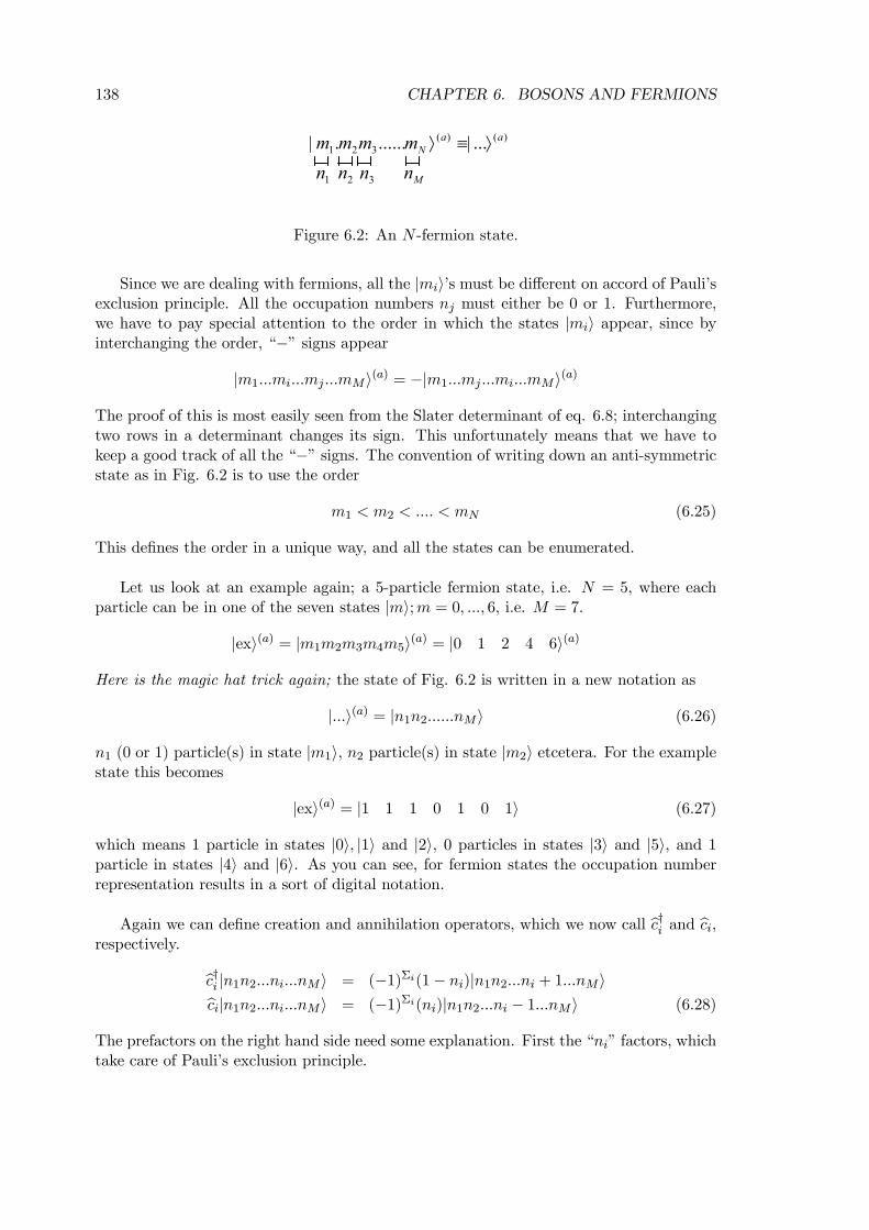
138 CHAPTER 6. BOSONS AND FERMIONS
1n Mn2n 3n
)()(321 ...|.......| aa
Nmmmm ⟩≡⟩
Figure 6.2: An N -fermion state.
Since we are dealing with fermions, all the |mii’s must be different on accord of Pauli’sexclusion principle. All the occupation numbers nj must either be 0 or 1. Furthermore,we have to pay special attention to the order in which the states |mii appear, since byinterchanging the order, “−” signs appear
|m1...mi...mj ...mMi(a) = −|m1...mj ...mi...mMi(a)
The proof of this is most easily seen from the Slater determinant of eq. 6.8; interchangingtwo rows in a determinant changes its sign. This unfortunately means that we have tokeep a good track of all the “−” signs. The convention of writing down an anti-symmetricstate as in Fig. 6.2 is to use the order
m1 < m2 < .... < mN (6.25)
This defines the order in a unique way, and all the states can be enumerated.
Let us look at an example again; a 5-particle fermion state, i.e. N = 5, where eachparticle can be in one of the seven states |mi;m = 0, ..., 6, i.e. M = 7.
|exi(a) = |m1m2m3m4m5i(a) = |0 1 2 4 6i(a)
Here is the magic hat trick again; the state of Fig. 6.2 is written in a new notation as
|...i(a) = |n1n2......nMi (6.26)
n1 (0 or 1) particle(s) in state |m1i, n2 particle(s) in state |m2i etcetera. For the examplestate this becomes
|exi(a) = |1 1 1 0 1 0 1i (6.27)
which means 1 particle in states |0i, |1i and |2i, 0 particles in states |3i and |5i, and 1particle in states |4i and |6i. As you can see, for fermion states the occupation numberrepresentation results in a sort of digital notation.
Again we can define creation and annihilation operators, which we now call bc†i and bci,respectively.
bc†i |n1n2...ni...nMi = (−1)Σi(1− ni)|n1n2...ni + 1...nMibci|n1n2...ni...nMi = (−1)Σi(ni)|n1n2...ni − 1...nMi (6.28)
The prefactors on the right hand side need some explanation. First the “ni” factors, whichtake care of Pauli’s exclusion principle.
6.2. N PARTICLES; THE MODERN ERA 139
• If ni = 1, one cannot create another particle in the same state because of Pauli’sexclusion principle and if ni = 0 one can. The factor (1− ni) takes care of this.
• If ni = 0, one cannot annihilate a particle from this state per definition, but if ni = 1one can. The factor (ni) takes care of this.
The factors (−1)Σi come from a decent book keeping of signs. See also Mattuck, §7.3.One way to fix the sign-and-ordering problem is to let a creation operator bc†k always createits particle in a state at the left most position. In old-fashioned notation this reads
bc†k|m1m2....mN i(a) = |km1m2....mN i(a) (6.29)
where we have added one particle in state |ki to the N which were already present instates |m1i, |m2i, ..., |mNi. Note k must be different from any of the mi, otherwise weget zero. What happens is again best seen from the Slater determinant of eq. 6.8. Thecreation operation of eq. 6.29 adds an extra row and column. If k is equal to one of themi, two rows in the determinant are equal, and the determinant is zero.
bc†k¯¯ |m1 (1)i |m1 (2)i ... |m1 (N)i|m2 (1)i |m2 (2)i ... |m2 (N)i... ... ... ...
|mN (1)i |mN (2)i ... |mN (N)i
¯¯ =
¯¯¯|k (1)i |k (2)i ... ... |k (N + 1)i|m1 (1)i |m1 (2)i ... ... |m1 (N + 1)i|m2 (1)i |m2 (2)i ... ... |m2 (N + 1)i... ... ... ... ...
|mN (1)i |mN (2)i ... ... |mN (N + 1)i
¯¯¯
(we ignore the normalization constant for the moment). Since k can be any number, ingeneral the state of eq. 6.29 does not comply with the ordering defined by eq. 6.25. Wehave to “transport” k to its proper position; i.e. if mi−1 < k < mi then the correct orderis
|m1m2...mi−1kmi...mN i(a)
We can achieve this step by step from eq. 6.29 by interchanging k with its neighbor. Eachtime we do a “−” sign appears.
|km1m2....mN i(a) = −|m1km2....mNi(a) =(−1)2|m1m2k....mN i(a) = (−1)Σi |m1m2...mi−1kmi...mN i(a)
where Σi is the total number of states that are actually occupied and come before k inthe ordering of states. In other words
Σi = n1 + n2 + ...+ ni−1 (6.30)
A similar sign convention is handy for the annihilation operator bck. Here we do the stepsin reverse; first transport k to the left most position
|m1m2...mi−1kmi...mNi(a) = (−1)Σi |km1m2...mi−1mi...mN i(a)
and then annihilate the particle in this state
bck|km1m2....mN i(a) = |m1m2....mN i(a) (6.31)
In summary, the sign (−1)Σi is produced as follows
140 CHAPTER 6. BOSONS AND FERMIONS
1. We define the creation, annihilation operators bc†k,bck such that they always operateat the front of the anti-symmetric state |m1m2....mNi(a).
2. Then we reorder the states such that the rule of eq. 6.25 is obeyed.
The general result of all this book keeping is given by eq. 6.28. Apart from theprefactors, these fermion creation/annihilation operators look just like the boson ones ofeq. 6.17. This is however slightly misleading. There is one very (and I mean very, very)important difference. The fermion operators obey anti-commutation relations:hbci,bc†ji
+≡ bcibc†j + bc†jbci = δijhbc†i ,bc†ji
+= [bci,bcj ]+ = 0 (6.32)
Note the “+” sign; an extremely important difference with bosons ! The relations areeasily proved from the definitions, eq. 6.28 (see also Mattuck, p. 130). I will give oneexample, the rest you can easily prove yourself.
bcibc†i |n1n2...ni...nMi = (−1)Σi(1− ni)bci|n1n2...ni + 1...nMi= (−1)Σi(1− ni)(−1)Σi(ni + 1)|n1n2...ni...nMi= (1− n2i )|n1n2...ni...nMi
bc†ibci|n1n2...ni...nMi = (−1)Σinibc†i |n1n2...ni − 1...nMi= (−1)Σini(−1)Σi(1− ni + 1)|n1n2...ni − 1...nMi= (2ni − n2i )|n1n2...ni...nMi (6.33)
from which it follows
(bcibc†i + bc†ibci)|n1n2...ni...nMi = (1 + 2ni − 2n2i )|n1n2...ni...nMiSince ni can only be 0 or 1 (remember: fermions), 1 + 2ni − 2n2i = 1 and since this resultis true for any basis state, we have bcibc†i + bc†ibci = 1.
The difference in sign between the relations obeyed by fermion and by boson opera-tors, eq. 6.32 vs. eq. 6.17 reflects the sign difference we introduced in the |....i(a) and|....i(s) states, eq. 6.5 vs. eq. 6.3. This difference is very fundamental since it reflects theanti-symmetry or symmetry of the many-particle states, and thus the difference betweenfermions and bosons, the two fundamentally different kinds of elementary particles wefind in nature. You might already get some idea on the usefulness of second quantization.Instead of the “sign book keeping” you have to do when manipulating the complex expres-sions of the |....i(a) states, one can use the “sign rules” of the operator anti-commutationrelations of eq. 6.32. As always, operator algebra is simpler than manipulating states.In order to make explicit use of the power of second quantization, one has to expressoperators accordingly. Remarkably, the second quantization expressions for the one- andtwo-particle operators for fermions have exactly the same form as for bosons, cf. eq. 6.19
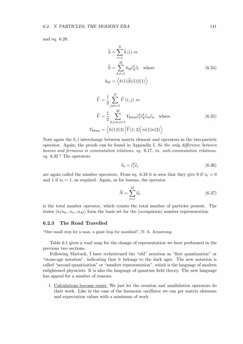
6.2. N PARTICLES; THE MODERN ERA 141
and eq. 6.20.
bh = NXi=1
bh (i)⇔bh = MX
k,l=1
hklbc†kbcl where (6.34)
hkl =Dk(1)|bh(1)|l(1)E
bV = 1
2
NXj 6=i=1
bV (i, j)⇔bV = 1
2
MXk,l,m,n=1
Vklmnbc†lbc†kbcmbcn where (6.35)
Vklmn =Dk(1)l(2)
¯ bV (1, 2)¯m(1)n(2)ENote again the k, l interchange between matrix element and operators in the two-particleoperator. Again, the proofs can be found in Appendix I. So the only difference betweenbosons and fermions is commutation relations, eq. 6.17, vs. anti-commutation relations,eq. 6.32 ! The operators
bni = bc†ibci (6.36)
are again called the number operators. From eq. 6.33 it is seen that they give 0 if ni = 0and 1 if ni = 1, as required. Again, as for bosons, the operator
bN =MXi=1
bni (6.37)
is the total number operator, which counts the total number of particles present. Thestates |n1n2...ni...nMi form the basis set for the (occupation) number representation.
6.2.3 The Road Travelled
“One small step for a man, a giant leap for mankind”, N. A. Armstrong.
Table 6.1 gives a road map for the change of representation we have performed in theprevious two sections.
Following Mattuck, I have rechristened the “old” notation as “first quantization” or“stone-age notation”, indicating that it belongs to the dark ages. The new notation iscalled “second quantization” or “number representation”, which is the language of modernenlightened physicists. It is also the language of quantum field theory. The new languagehas appeal for a number of reasons.
1. Calculations become easier. We just let the creation and annihilation operators dotheir work. Like in the case of the harmonic oscillator we can get matrix elementsand expectation values with a minimum of work.
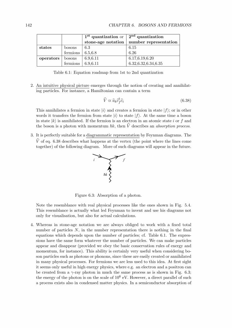
142 CHAPTER 6. BOSONS AND FERMIONS
1st quantization or 2nd quantizationstone-age notation number representation
states bosons 6.3 6.15fermions 6.5,6.8 6.26
operators bosons 6.9,6.11 6.17,6.19,6.20fermions 6.9,6.11 6.32,6.32,6.34,6.35
Table 6.1: Equation roadmap from 1st to 2nd quantization
2. An intuitive physical picture emerges through the notion of creating and annihilat-ing particles. For instance, a Hamiltonian can contain a term
bV ∝ bakbc†fbci (6.38)
This annihilates a fermion in state |ii and creates a fermion in state |fi; or in otherwords it transfers the fermion from state |ii to state |fi. At the same time a bosonin state |ki is annihilated. If the fermion is an electron in an atomic state i or f andthe boson is a photon with momentum ~k, then bV describes an absorption process.
3. It is perfectly suitable for a diagrammatic representation by Feynman diagrams. ThebV of eq. 6.38 describes what happens at the vertex (the point where the lines cometogether) of the following diagram. More of such diagrams will appear in the future.
i f
k
Figure 6.3: Absorption of a photon.
Note the resemblance with real physical processes like the ones shown in Fig. 5.4.This resemblance is actually what led Feynman to invent and use his diagrams notonly for visualisation, but also for actual calculations.
4. Whereas in stone-age notation we are always obliged to work with a fixed totalnumber of particles N , in the number representation there is nothing in the finalequations which depends upon the number of particles; cf. Table 6.1. The expres-sions have the same form whatever the number of particles. We can make particlesappear and disappear (provided we obey the basic conservation rules of energy andmomentum, for instance). This ability is certainly very useful when considering bo-son particles such as photons or phonons, since these are easily created or annihilatedin many physical processes. For fermions we are less used to this idea. At first sightit seems only useful in high energy physics, where e.g. an electron and a positron canbe created from a γ-ray photon in much the same process as is shown in Fig. 6.3;the energy of the photon is on the scale of 106 eV. However, a direct parallel of sucha process exists also in condensed matter physics. In a semiconductor absorption of
6.3. THE PARTICLE-HOLE FORMALISM 143
a photon across the band gap creates an electron (in the conduction band) and ahole (in the valence band); here the energy of the photon is on the scale of the bandgap, i.e. 1 eV.4,5
6.3 The Particle-Hole Formalism
“Entia non sunt multiplicanda praeter necessitatem”, William Occam (No more things should be
assumed to exist than necessary).
Each fermion occupies a different state according to Pauli. Filling a system withfermions (e.g. electrons in a molecule or crystal), the system being in thermal equilibriumat not too high a temperature, is like filling a bucket with water. The lowest level isfilled first, then the next lowest level etcetera. In a large system one fills energy levelswhich are distributed over a range over tens or even hundredths of eV’s. In many (optical,electrical transport) experiments we only probe the energy levels in a range of a few eVaround the highest occupied one. So it is a nuisance to have to drag along all these verylow lying energy levels which never change their occupation. To avoid this nuisance, thesecond quantization formalism for fermions can be adapted somewhat. This adaptation iscalled the particle-hole formalism. As usual, it is not only a formalism, but it also paintsa new physical picture. How the particle-hole formalism works is best explained using apet model of solid state physics, the so-called homogeneous electron gas. As much as theharmonic oscillator or quantum chain is the prime example of a many-boson system, thehomogeneous electron gas is the prime example of a many-fermion system.
6.3.1 The Homogeneous Electron Gas
The homogeneous electron gas consists of an infinite number of electrons in infinite space,such that their average density is a fixed ρ. To make the whole system neutral, the electronsmove in a fixed, positively charged background which has the same charge density ρ. Thepositive background is necessary, otherwise the Coulomb repulsion between the infinitenumber of electrons would lead to an infinite positive energy. The homogeneous electrongas is also called “jellium”; it is the metallic equivalent of a homogeneous medium. It isalso a simple model for a metal, in which the positive charge of the nuclei or ion cores of themetal is smeared out homogeneously over the background. The model is far less academicthan might seem at first sight; it turns out to be quite a reasonable first approximationfor many metals.
In this section we will consider the so-called non-interacting electron gas. That is, weneglect all the electron-electron Coulomb repulsions. Since this repulsion is very large,this may seem not at all appropriate. In fact, it is not at all appropriate, but we will
4Hendrik Casimir was a famous dutch physicist who could (should?) have, but unfortunately did notget the nobel prize. He mentions that Dirac’s electron-positron concept might have been inspired by theelectron-hole concept in semiconductors. H. B. G. Casimir, Het toeval van de werkelijkheid, (Meulenhoff,Amsterdam, 1983) bevat de memoires van Casimir. Het is een leuk boek, vol anecdotes over mensen engebeurtenissen uit de begindecennia van de quantum mechanica. Het bevat o.a. zijn fameuze lezing over“broken English”, de internationale taal van de wetenschap waarin ook deze lecture notes zijn geschreven.
5The difference in energy scale of at least six orders of magnitude between condensed matter and highenergy physics means that we have to use relativistic quantum mechanics for the latter, whereas we canstick to non-relativistic quantum mechanics (i.e. the Schrodinger equation) for the former.
144 CHAPTER 6. BOSONS AND FERMIONS
show in the last chapter how to introduce the Coulomb repulsion in a way such that thephysics of the interacting electron gas resembles that of the non-interacting electron gas(by transforming particles into quasi-particles). We will leave that subject until later andstick to the non-interacting gas for the moment. The Hamiltonian is
bh =Xi
bp2i2me
+ bV (6.39)
The first term is the sum of kinetic energies of all the electrons. The second term is thepotential due to the uniform positive background. Since it is just a constant, we can
neglect it. The eigenstates of the single particle Hamiltonian bp22me
are written as usual as|ki; they are also the eigenstates of the momentum operator.
bp|ki = ~k|kibp22me
|ki = ²k|ki with ²k =~2|k|22me
(6.40)
In the position representation, these momentum eigenstates are of course plane waves, asin Chapter 4, see Section 4.2
hr|ki = 1√Ωeik·r ≡ φk(r) (6.41)
We are using a periodic box of volume Ω again to normalize these states and produce adiscrete spectrum in k. Electrons are fermions and we use these single particle states toform anti-symmetric states for N particles; or, in stone-age notation6
|k1k2....kN i(a) (6.42)
Filling the system with electrons, we start from the lowest energy level ²k = 0 for k =(0, 0, 0), see eq. 6.40. All states |ki for which k has the same length |k| have the sameenergy ²k. So filling the levels according to increasing energy ²k fills up spherical shells,when we make a plot in k-space. This is shown in Fig. 6.4.The plot is in two dimensionsk = (kx, ky); in three dimensions k = (kx, ky, kz) the shells will of course be spheres.
In the ground state of our homogeneous electron gas all states k with ²k ≤ ²F will beoccupied and all states with ²k > ²F will be unoccupied.
7 ²F is called the Fermi energy.We can write it as
²F =~2k2F2me
(6.43)
6Electrons also have a spin. In this course we will not be looking at any processes in which an interactionwith the electronic spin takes place. Under these circumstances, spin is then a “silent” quantum number,and electrons behave just like spinless particles. Only when counting electrons we have to take intoconsideration that each state |ki can in fact hold two electrons, one with spin up, and one with spin down.Keeping this in the back of our mind, we will not use an explicit notation for the spin quantum number.If one wishes to explicitly specify the spin state, one can always substitute |ki by |k;σzi = |ki|σzi withσz = ± 1
2.
7That is at zero temperature. At a finite temperature, there will be some thermal excitations, givingrise to the Fermi-Dirac distribution you know from your statistical physics course. Since usually ²F & 10eV and kT ≈ 0.026 eV at room temperature, the effect of thermal excitations on the occupation numbersof the levels is small, except for very high temperatures.
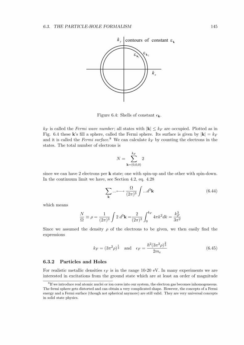
6.3. THE PARTICLE-HOLE FORMALISM 145
xk
yk kεconstant of contours
1kε 2k
ε
Figure 6.4: Shells of constant ²k.
kF is called the Fermi wave number ; all states with |k| ≤ kF are occupied. Plotted as inFig. 6.4 these k’s fill a sphere, called the Fermi sphere. Its surface is given by |k| = kFand it is called the Fermi surface.8 We can calculate kF by counting the electrons in thestates. The total number of electrons is
N =
kFXk=(0,0,0)
2
since we can have 2 electrons per k state; one with spin-up and the other with spin-down.In the continuum limit we have, see Section 4.2, eq. 4.28X
k
...←→ Ω
(2π)3
Z...d3k (6.44)
which means
N
Ω≡ ρ =
1
(2π)3
Z2 d3k =
2
(2π)3
Z kF
04πk2dk =
k3F3π2
Since we assumed the density ρ of the electrons to be given, we then easily find theexpressions
kF = (3π2ρ)
13 and ²F =
~2(3π2ρ)23
2me(6.45)
6.3.2 Particles and Holes
For realistic metallic densities ²F is in the range 10-20 eV. In many experiments we areinterested in excitations from the ground state which are at least an order of magnitude
8If we introduce real atomic nuclei or ion cores into our system, the electron gas becomes inhomogeneous.The fermi sphere gets distorted and can obtain a very complicated shape. However, the concepts of a Fermienergy and a Fermi surface (though not spherical anymore) are still valid. They are very universal conceptsin solid state physics.
146 CHAPTER 6. BOSONS AND FERMIONS
smaller in energy, Eexc ¿ 1 eV. The majority of states with energies below ²F −Eexc areuntouched by the experiment and it is a nuisance to drag them along. For that reason weintroduce the particle-hole formalism (see also Mattuck §4.2, 4.3, and 7.5). We define twosets of new fermion creation/annihilation operators for electrons and holes, respectively,which are related to our previous fermion operators of eqs. 6.28 and 6.32 as
ba†k = bc†k ; bak = bck if |k| > kF (electrons)bb†k = bck ; bbk = bc†k if |k| ≤ kF (holes) (6.46)
For energies above ²F the operators ba†k,bak correspond to creating an electron in a state |ki,with |k| > kF just as before (such states are unoccupied in the ground state). However,for energies below ²F the annihilation of an electron by bck is now associated with thecreation of a hole by bb†k (which makes sense, we are creating a hole in a state which isoccupied in the ground state). The annihilation of a hole by bbk is then obviously associatedwith creating an electron by bc†k. The bak’s and bbk’s must obey the same anti-commutationrelations as the bck’s, see eq. 6.32.hbak,ba†k0i
+= δk,k0 ;
hbbk,bb†k0i+= δk,k0 etcetera (6.47)
Furthermore the bak’s and bbk’s always anti-commute, since they are related to bck’s withdifferent k’s, eq. 6.46. hbak,bbk0i
+= 0 etcetera (6.48)
The Hamiltonian in bc†kbck-number representation is given bybh =Xk0,k
hk0kbc†k0bcksince the Hamiltonian of eq. 6.39 only contains a one-particle operator. We have
hk0k = hk0(1)|bh(1)|k(1)i = hk0(1)| bp212me
|k(1)i= ²khk0|ki = ²kδk0,k
see eq. 6.40.9. The Hamiltonian thus becomes
bh =Xk
²kbc†kbck (6.49)
In bak’s and bbk’s we getbh =
X|k|≤kF
²kbbkbb†k + X|k|>kF
²kba†kbak=
X|k|≤kF
²k −X|k|≤kF
²kbb†kbbk + X|k|>kF
²kba†kbak9Note the index (1) is used as a dummy index. We usually discard it when there is no confusion.
6.3. THE PARTICLE-HOLE FORMALISM 147
where we have obtained the last line by using the anti-commutation rule bbkbb†k+bb†kbbk = 1.We can give this expression a new interpretation. First note that
E0 =X|k|≤kF
²k (6.50)
is the sum of energies of all states occupied in the ground state, i.e. the ground state energy.
Here comes the main idea: we consider the ground state as the new reference pointfrom which we create and annihilate particles. So we consider the ground state, being thelowest energy state of a system of fermions, as our new vacuum state ! The Hamiltonianis written as bh = E0 − X
|k|≤kF²kbb†kbbk + X
|k|>kF²kba†kbak (6.51)
Since ba†kbak = bnk are number operators, according to eq. 6.36, the last term of thisexpression counts the number of electrons present with energies above the Fermi level.Each electron can be assigned an energy ²k and a momentum ~k. The second term alsocontains number operators bb†kbbk. It counts the number of a new kind of particle, whichis present below the Fermi level, and has an energy −²k. Originally it corresponded tothe annihilation of an electron with energy ²k; so taking away an electron with energy²k corresponds to creating a “new particle” with energy −²k. From the standpoint ofconservation of energy this makes perfect sense. Similarly one can argue that taking awayan electron with momentum ~k and charge −e corresponds to creating a new particlewith momentum −~k and charge +e (consider the laws of conservation of momentum andcharge). The Hamiltonian part
bhh = − X|k|≤kF
²kbb†kbbkhas the same form as eq. 6.49. Since the latter has been derived from eq. 6.39, bhh has thesame eigenstates, cf. eqs. 6.40 and 6.42, the only difference being the “−” sign in front ofthe eigenvalues −²k. In particular, the “new particle” has the same wave functions of eq.6.41. As you have guessed by now, the “new particle” created by bb†k is called a hole.SUMMARY
In the particle-hole formalism, both particles and hole are created from the vacuum. Thevaccuum has the following properties
• The vacuum state is the ground state of the electron gas.
• The energy of the vacuum is the ground state energy E0, given by eq. 6.50.
Particles (electrons) are created above the Fermi level; holes are created below theFermi level. Table 6.2 gives a comparison between the properties of particles and holes.
The particle-hole formalism describes both electrons and holes as additions to theground state, or in more fancy words as excitations of the vacuum. The electron is calleda particle, and its counter part the hole is called an anti-particle. The particle/anti-particleidea is quite universal and commonplace.
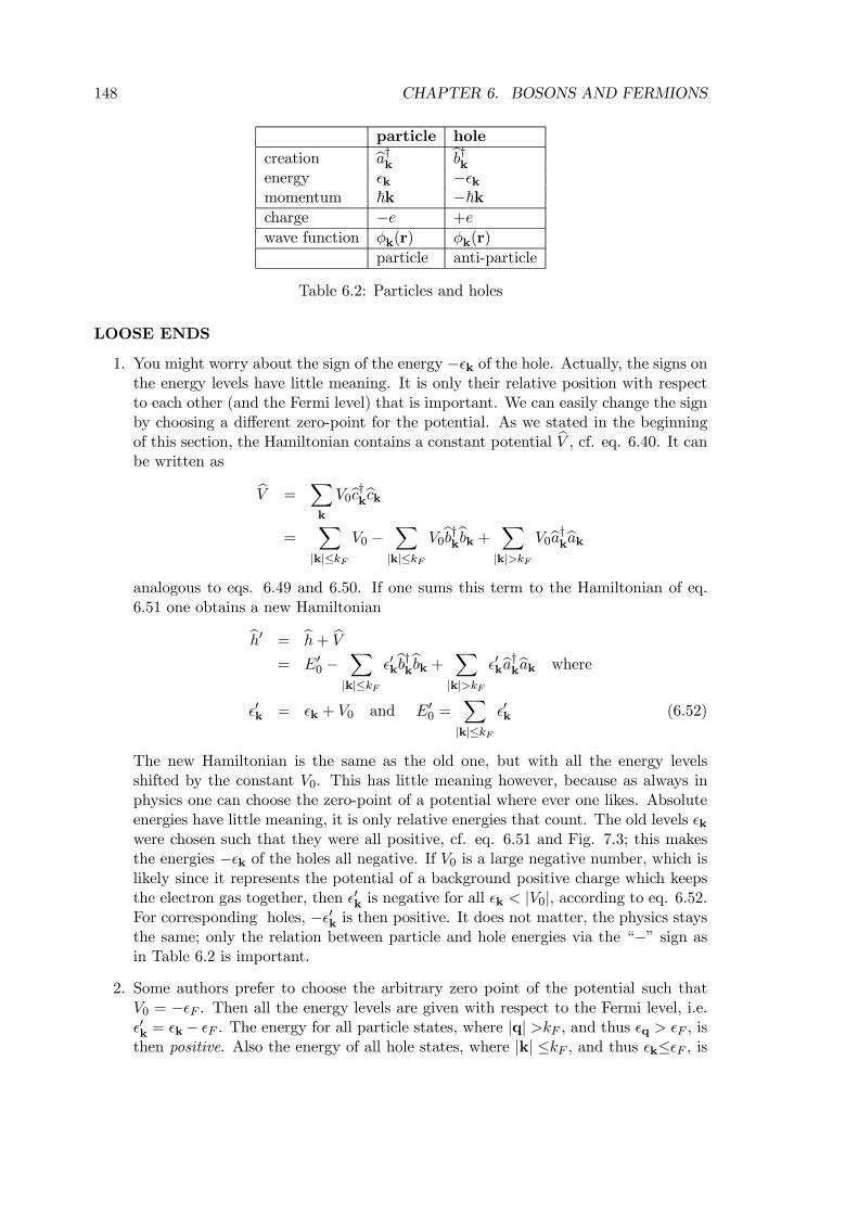
148 CHAPTER 6. BOSONS AND FERMIONS
particle hole
creation ba†k bb†kenergy ²k −²kmomentum ~k −~kcharge −e +e
wave function φk(r) φk(r)
particle anti-particle
Table 6.2: Particles and holes
LOOSE ENDS
1. You might worry about the sign of the energy −²k of the hole. Actually, the signs onthe energy levels have little meaning. It is only their relative position with respectto each other (and the Fermi level) that is important. We can easily change the signby choosing a different zero-point for the potential. As we stated in the beginningof this section, the Hamiltonian contains a constant potential bV , cf. eq. 6.40. It canbe written as bV =
Xk
V0bc†kbck=
X|k|≤kF
V0 −X|k|≤kF
V0bb†kbbk + X|k|>kF
V0ba†kbakanalogous to eqs. 6.49 and 6.50. If one sums this term to the Hamiltonian of eq.6.51 one obtains a new Hamiltonianbh0 = bh+ bV
= E00 −X|k|≤kF
²0kbb†kbbk + X|k|>kF
²0kba†kbak where
²0k = ²k + V0 and E00 =X|k|≤kF
²0k (6.52)
The new Hamiltonian is the same as the old one, but with all the energy levelsshifted by the constant V0. This has little meaning however, because as always inphysics one can choose the zero-point of a potential where ever one likes. Absoluteenergies have little meaning, it is only relative energies that count. The old levels ²kwere chosen such that they were all positive, cf. eq. 6.51 and Fig. 7.3; this makesthe energies −²k of the holes all negative. If V0 is a large negative number, which islikely since it represents the potential of a background positive charge which keepsthe electron gas together, then ²0k is negative for all ²k < |V0|, according to eq. 6.52.For corresponding holes, −²0k is then positive. It does not matter, the physics staysthe same; only the relation between particle and hole energies via the “−” sign asin Table 6.2 is important.
2. Some authors prefer to choose the arbitrary zero point of the potential such thatV0 = −²F . Then all the energy levels are given with respect to the Fermi level, i.e.²0k = ²k− ²F . The energy for all particle states, where |q| >kF , and thus ²q > ²F , isthen positive. Also the energy of all hole states, where |k| ≤kF , and thus ²k≤²F , is
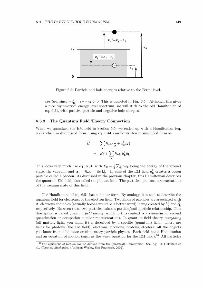
6.3. THE PARTICLE-HOLE FORMALISM 149
Fε
0
εk
εq
' Fε ε ε= −q q
' Fε ε ε− = −k k
Fε
0
εk
εq
' Fε ε ε= −q q
' Fε ε ε− = −k k
Figure 6.5: Particle and hole energies relative to the Fermi level.
positive, since −²0k = ²F − ²k > 0. This is depicted in Fig. 6.5. Although this givesa nice “symmetric” energy level spectrum, we will stick to the old Hamiltonian ofeq. 6.51, with positive particle and negative hole energies.
6.3.3 The Quantum Field Theory Connection
When we quantized the EM field in Section 5.5, we ended up with a Hamiltonian (eq.5.79) which in discretized form, using eq. 6.44, can be written in simplified form as
bH =Xk
~ωk(1
2+ ba†kbak)
= E0 +Xk
~ωk ba†kbakThis looks very much like eq. 6.51, with E0 =
12
Pk ~ωk being the energy of the ground
state, the vacuum, and ²k = ~ωk = ~c|k|. In case of the EM field ba†k creates a bosonparticle called a photon. As discussed in the previous chapter, this Hamiltonian describesthe quantum EM field, also called the photon field. The particles, photons, are excitationsof the vacuum state of this field.
The Hamiltonian of eq. 6.51 has a similar form. By analogy, it is said to describe thequantum field for electrons, or the electron field. Two kinds of particles are associated withit; electrons and holes (actually holons would be a better word), being created by ba†k and bb†krespectively. Between these two particles exists a particle/anti-particle relationship. Thisdescription is called quantum field theory (which in this context is a synonym for secondquantization or occupation number representation). In quantum field theory everything(all matter, light, you name it) is described by a specific (quantum) field. There arefields for photons (the EM field), electrons, phonons, protons, etcetera; all the objectsyou know from solid state or elementary particle physics. Each field has a Hamiltonianand an equation of motion (such as the wave equation for the EM field).10 All particles
10The equations of motion can be derived from the (classical) Hamiltonian. See, e.g., H. Goldstein etal., Classical Mechanics, (Addison Wesley, San Francisco, 2002).
150 CHAPTER 6. BOSONS AND FERMIONS
mentioned are excitations of (the vacuum state of) their quantum field. Bosons fields likethe EM field, have only one kind of particle. Fermion fields, like the electron field, havetwo kinds of particle; a particle and an anti-particle. This point of view carries over fromcondensed matter physics to high energy physics, which each have their own elaborate setsof particles and anti-particles.11
So far, we have been considering particles that do not interact with each other. Thiswould make the world very easy to understand, but also very boring. However,
• Fields of a different kind can interact with each other. For instance, electrons interactwith photons; Figs. 3.2, 5.5, 6.3. It is custom in such diagrams to represent fermionsby solid lines and bosons by “wavy” lines or dashed lines.
• Particles of one field can interact with each other. For instance, eqs. 6.20 and 6.21describes the Coulomb repulsion between electrons.
6.4 Second Quantization and the Electron Field
In this section I want to spend some words on the origin of this seemingly strange phrase“second quantization”. When we quantized the electro-magnetic (EM) field in free spacewe had a classical wave equation to start from, which can be derived from Maxwell’sequation, cf. Section 5.5. For the vector potential A (r, t) it reads
∇2A (r, t)− 1
c2∂2A (r, t)
∂t2= 0 (6.53)
and we derived its general solution (cf. eqs. 5.68 and 5.69)
A (r, t) =
√Ω
(2π)3
Xs=1,2
Zd3k Ak,s(t) εk,se
ik·r (6.54)
The functions eik·r are the modes in free space; εk,s are the polarization vectors; and thecoefficients Ak,s are the amplitudes. The time dependence of the latter has the generalform
Ak,s(t) = ak,se−iωkt + a∗−k,se
iωkt (6.55)
and in order that eqs. 6.54 and 6.55 give the solution to eq. 6.53, the dispersion relationis
ωk = c|k| (6.56)
The move from classical electrodynamics to quantum electrodynamics was made by makingthe amplitudes quantum operators
Ak,s → bqk,s (6.57)
11The physics can be slightly different, however. In high energy physics, one can also have boson fieldsthat have particles and anti-particles
6.4. SECOND QUANTIZATION AND THE ELECTRON FIELD 151
and leaving all the other classical objects and relations untouched. From there on, all wehad to do to derive the states of the quantum EM field (photons), is to use eq. 6.57 totransform the classical energy into a quantum mechanical Hamiltonian.
Now consider the following equation
− ~2
2m∇2ψ (r, t)− i~∂ψ (r, t)
∂t= 0 (6.58)
We immediately recognize this as the Schrodinger wave equation of a single electron infree space. Its general solution can be described in the same way as in eq. 6.54, i.e. as aFourier integral.
ψ (r, t) =
√Ω
(2π)3
Zd3k ck(t) e
ik·r (6.59)
where we recognize eik·r as the eigenfunctions for the free electron, which we can interpreteas the “modes”. The coefficients ck(t) then give the amplitudes and phases, as before.There are however a couple of differences with the EM field.
1. Since ψ (r, t) is a scalar function, and not a vector function like A (r, t) we need nopolarization vectors.
2. The time dependence of its amplitudes are given by
ck(t) = cke−iωkt (6.60)
In order that eqs. 6.59 and 6.60 present a solution to the Schrodinger equation ofeq. 6.58, the dispersion relation must be
~ωk =~2|k|22m
(6.61)
The latter is of course the familiar relation between energy and momentum E = p2
2m ifone accepts Planck18’s and De Broglie29’s relations E = ~ω, and p = ~k. The fact that therelation between frequency and wave number has to be quadratic instead of simply linearas in eq. 6.53 urged Schrodinger to derive a “wave” equation which has a first order timederivative, cf. eq. 6.58, instead of the second order time derivative of a conventional waveequation like eq. 6.53. Of course he also had to put an “i” in front of the time derivative,since otherwise it would not have been a wave equation, but a “diffusion” equation whichonly has non-wave like e±κ·r solutions.
Now suppose poor me is just a simple chemist who does not understand quantummechanics very deeply.12 I have missed all the introductory courses in quantum mechanicsand I just heard about quantizing the EM field following the prescription going from eqs.6.53 to 6.57. Being faced with eq. 6.58, I am thinking that this is just a “classical”wave equation like eq. 6.53. The function ψ (r, t) then plays the role of a classical wave,or classical field as in the previous chapter. It is a scalar, and not a vector like the
12All three statements are true.
152 CHAPTER 6. BOSONS AND FERMIONS
EM potential, but that makes it only simpler. It describes electrons, so I am told bySchrodinger, so I call it the “classical” electron field. You know that this is wrong, sinceyou are experts in quantum mechanics, but stay with me for the sake of the argument.I think I know how to quantize this “classical” electron field. I simply follow the sameprescription of quantum electrodynamics and turn the amplitudes into operators
ck → bck (6.62)
One of my clever fellow students told me that the energy an electron wave can be calculatedas
E =
Zd3r ψ∗ (r, t)
·− ~
2
2m∇2¸ψ (r, t) (6.63)
Using eq. 6.59 and doing some δ-function manipulation as in the previous chapter thiscan be rewritten as
E =Ω
(2π)3
Zd3k ~ωk c∗kck (6.64)
with ~ωk given by eq. 6.61. This looks fine by me; essentially it is just Planck’s relationapplied to each mode, and all modes are summed over using their “intensity” |ck|2 asweight factors. So now I say, let’s turn this “classical” energy into a quantum mechanicalHamiltonian by using the prescription of eq. 6.62.
bH =Ω
(2π)3
Zd3k ~ωk bc†kbck (6.65)
But this looks just like the Hamiltonian in number representation of the homogeneouselectron gas, cf. eq. 6.49 ! We have to set ~ωk = ²k, but that is o.k. if we compare eqs.6.40 and 6.61. Furthermore, we have switched from a sum over k to an integral, i.e. froma discrete to a continuous spectrum. But we have done this before; it poses no problems.Switching back to a discrete spectrum in a box using eq. 6.44, we get eq. 6.49
bH =Xk
~ωkbc†kbckSince the bck’s are operators, we have to figure out what their algebra is, i.e. their(anti)commutation relations. But that is what we have been doing in this chapter allalong, so we already know the answer: since electrons are fermions, the bck’s are re-quired to obey the anti-commutation rules of eq. 6.32. I have found the solution forthe quantum electron field (see also Mattuck, the end of chapter 7). For the EM field this
procedure gave the many photon states. Each photon can be created by an operator ba†kworking on the (photon) vacuum and in this sense it is called an excitation of the EM field.
Similarly, each electron is created by an operator bc†k working on the (electron) vacuum; itcan be called an excitation of the electron field.
Now of course, after I did all this work, you come and tell me that the Schrodinger waveequation, eq. 6.58, is in fact not a “classical” wave equation at all, but a quantum waveequation. No problem, I say, let’s call the Schrodinger wave equation first quantization andthe step of eq. 6.62, or equivalently the step from eq. 6.64 to 6.65, second quantization.
6.4. SECOND QUANTIZATION AND THE ELECTRON FIELD 153
The result of quantizing the amplitudes ck of the modes of the Schrodinger wave equationis a many-body Hamiltonian in second quantized form. Since that is exactly what we havebeen deriving in this chapter all along, the procedure must be right. Such are the wondersof quantum field theory.
Note that we just as well could have made the substitution of eq. 6.62 in eq. 6.59.From the latter (and its complex conjugate) the so-called electron field operators bψ (r, t)and bψ† (r, t) are defined as
bψ (r, t) =
√Ω
(2π)3
Zd3k bck(t) eik·r ; bck(t) = bcke−iωkt
bψ† (r, t) =
√Ω
(2π)3
Zd3k bc†k(t) e−ik·r ; bc†k(t) = bc†keiωkt (6.66)
They play a similar role for the quantum electron field as the electric and magnetic fieldoperators in the EM theory, cf eq. 5.75 in Section 5.5, Chapter 5. The Hamiltonian thenbecomes
bH =
Zd3r bψ† (r, t) ·− ~2
2m∇2¸ bψ (r, t) (6.67)
by (second) quantization of eq. 6.63. One can easily check that this is equivalent to eq.6.65. The annihiliation operator bck “lowers the amplitude of the wave” by annihilating aparticle in the mode characterized by wave vector k, cf. eq. 6.59. The creation operatorbc†k obviously creates a particle in this mode. According to eq. 6.41 one can also write
bc†k|0i→ |ki (6.68)
where the left hand side is in second quantization, and the right hand side is in stone-agenotation. Then also, using eqs. 6.66
bψ† (r) |0i =
Zd3k e−ik·r bc†k|0i = Z d3k e−ik·r |ki
=
Zd3k hk|ri |ki = |ri (6.69)
(apart from normalization factors). Thus the electron field operator bψ† (r) creates a par-ticle at a position r. The electron field operator bψ (r) then annihilates a particle at aposition r.
Obviously I did not think of this myself; the quantum field procedure is a classic inquantum mechanics by now. You can start from a wave-like equation like eqs. 6.53 or6.58 and find the solution in terms of modes, eqs. 6.54 or 6.59. Then you quantize theamplitudes, eqs. 6.57 or 6.62 and use this to construct a quantum Hamiltonian from the“classical” energy, eqs. 5.76 or 6.63. In case the wave equation is already quantum me-chanical, such as the Schrodinger equation, you call it “first quantization” and quantizingthe amplitudes “second quantization”. The eigenstates of the resulting Hamiltonian, eqs.5.77 or 6.65, are many-particle states. The nature of the particles, whether they are bosonsor fermions, is only determined by the algebra of their creation/annihilation operators,
154 CHAPTER 6. BOSONS AND FERMIONS
i.e. whether these commutate or anti-commutate. It works for any kind of wave equationand any kind of particle in any kind of physics (condensed matter, high energy, etcetera).I think that, in view of the cumbersome algebra required for the stone-age quantum way(see also Appendix I), we can all agree that this simple route followed by quantum fieldtheory is much faster. Moreover it applies to situations such as the EM field, in which thestone-age quantum route to many particles by first quantization does not work. For theEM field, “first quantization” gives the modes of the classical wave equation. It is only“second quantization” that gives you photons and quantum mechanics.
6.5 Appendix I. Identical Particle Algebra
In this Appendix I have gathered the bulk of the algebra that is needed to prove someof the statements made it in the text. In the first subsection it is proved that different(anti)symmetric states are orthogonal, and the normalization factors are calculated. Inthe second subsection the second quantization form of the operators given in the text isproved to be correct. The algebra is lengthy, but straight-forward, as the textbook clichestates.
6.5.1 Normalization Factors and Orthogonality
The factors Ns and Na are defined such that the states |....i(s) and |....i(a) are normalized;i.e. (s)h....|....i(s) = 1 and (a)h....|....i(a) = 1, cf. eqs. 6.3, 6.5 and 6.7. We do the anti-symmetric state first. Calculating (a)h....|....i(a) by the right hand side of eq. 6.5, leads toa double summation over permutations
PbP, bP 0 which has (N !)2 terms. These terms canbe divided into two classes
1. bP 6= bP 0; the “ off-diagonal” terms. The corresponding matrix element in (a)h....|....i(a)is
h bPm1 (1)m2 (2) ....mN (N) | bP 0m1 (1)m2 (2) ....mN (N)iBecause the two permutations bP, bP 0 are different from one another, there is at leastone particle i where on the left (the bra) side we have hmj(i)| and on the right (theket) side we have |mk(i)i, where mj 6= mk. (Note that because of Pauli’s exclusionprinciple all the numbers mi; i = 1, ..., N must be different from one another). Ifwe work out this matrix element as in Section 1.4, eq. 1.26, we see that this leadsto a factor hmj(i)|mk(i)i = 0, since the single particle basis set we started from isorthogonal. In conclusion, all “off-diagonal” terms give a zero contribution.
2. bP = bP 0; the “ diagonal” terms. These are all of the same typehm1m2....mN |m1m2....mNi = hm1|m1ihm2|m2i...hmN |mNi = 1
because our single particle basis set is orthonormal. Since there are N ! possiblepermutations, there are N ! of these “diagonal” terms.
Combining all the terms gives
(a)h....|....i(a) = (Na)2XbP, bP 0
= (Na)2N ! = 1
6.5. APPENDIX I. IDENTICAL PARTICLE ALGEBRA 155
and thus the normalization factor is
Na = 1√N !
(6.70)
Along the same lines one can prove
(a)hm01m02....m
0N |m1m2....mNi(a) =
NYk=1
δm0k,mk
(6.71)
i.e. the various anti-symmetric states are orthogonal. It goes as
(a)hm01m
02....m
0N |m1m2....mN i(a) =
(Na)2XbP, bP 0
(−1)p+p0h bP 0m01 (1)m02 (2) ....m
0N (N) | bPm1 (1)m2 (2) ....mN (N)i =
(Na)2XbP(−1)2ph bPm0
1 (1)m02 (2) ....m
0N (N) | bPm1 (1)m2 (2) ....mN (N)i =
(Na)2N !NYk=1
δm0k,mk
The step from the second to the third line can be made because we have defined the anti-symmetric state such that m1 < m2 < ... < mN and m01 < m0
2 < ... < m0N . This means
that the “off-diagonal” terms certainly give zero contribution (check this yourself). The“diagonal” terms all give the same contribution, and there are N ! of them.
For the symmetric state |....i(s) things are a bit trickier, since some of the numbersmi; i = 1, ... can be the same (there is no Pauli principle for bosons). Suppose we have astate
|m1 (1)m1 (2) ...m1(n1)m2(n1 + 1)...m2(n1 + n2)...mM (N)ii.e. n1 particles in state |m1i, n2 particles in state |m2i etcetera. The sum over all N !permutations
PbP in eq. 6.3 then contains onlyN !
n1!n2!...nM !
distinct terms (assuming we have onlyM different statesmi), since interchanging particleswhich are in the same state does not give a new term. When we calculate (s)h....|....i(s),there are again two types of terms in the double sum
PbP, bP 0 .1. The “ off-diagonal” terms between states which are distinct in the sense describedabove. This all give zero for the same reason as in the case of the anti-symmetricstate. They always contain a factor of type hmj(i)|mk(i)i where mj 6= mk.
2. The “ diagonal” terms between states which are not distinct in the sense describedabove. There are a whole bunch of them which result from permutating particleswhich are in the same state. Permutating the n1 particles in state |m1i gives n1!terms, all identical. In the double sum these give (n1!)
2 matrix elements. All thesematrix elements are 1, as before, because we have an orthonormal basis. We can dothe same with permuting the n2 particles in state |m2i, etcetera. These terms thusgive a contribution (n1!)
2(n2!)2...(nM !)
2
156 CHAPTER 6. BOSONS AND FERMIONS
Since we have N !n1!n2!...nM !
of these “diagonal” terms which give a contribution (n1!)2(n2!)
2...(nM !)2,
we get
(s)h....|....i(s) = (Ns)2XbP , bP 0
= (Ns)2 N !
n1!n2!...nM !(n1!)
2(n2!)2...(nM !)
2 = 1
and thus the normalization factor is
Ns = 1√N !n1!n2!...nM !
(6.72)
The orthogonality of the symmetric states is proved along the same lines
(s)hm01m
02....m
0N |m1m2....mNi(s) =
NYk=1
δm0k,mk
(6.73)
6.5.2 Second Quantization for Operators
Here we prove that the second quantization form of the operators given in the text, i.e.eqs. 6.19, 6.20, 6.34, and 6.35, is correct. The proof proceeds by showing that the matrixelements of operators in stone-age form, eq. 6.9—6.12 are identical to the matrix elementsof operators in second quantized form. Since this holds for any possible matrix element,and the states form a basis set, this proves that the two operator form are identical.Calculating matrix elements in stone-age form is the largest task. It can be shortened alittle bit by using a trick in which one initially considers special states only, and only inthe final stage one generalizes the result.
Stone-age Matrix Elements
First we will consider how one- and two-particle operators work on simple product statesin stone-age notation. A typical matrix element of a one-particle operator is
hm01 (1)m02 (2) ....m
0N (N) |
NXi=1
bh (i) |m1 (1)m2 (2) ....mN (N)i
=NXi=1
hm0i (i) |bh (i) |mi (i)i
Yk 6=ihm0
k (k) |mk (k)i
=NXi=1
hm0i (i) |bh (i) |mi (i)i
Yk 6=i
δm0k,mk
(6.74)
6.5. APPENDIX I. IDENTICAL PARTICLE ALGEBRA 157
by a straight-forward generalization of eq. 1.28 in Section 1.4. In a similar way one canshow that a matrix element of a two-particle operator becomes
hm01 (1)m
02 (2) ....m
0N (N) |
1
2
NXj 6=i=1
bV (i, j) |m1 (1)m2 (2) ....mN (N)i
=1
2
NXj 6=i=1
hm0i (i)m
0j (j) |bV (i, j) |mi (i)mj (j)i
Yk 6=i,k 6=j
hm0k (k) |mk (k)
=1
2
NXj 6=i=1
hm0i (i)m
0j (j) |bV (i, j) |mi (i)mj (j)i
Yk 6=i,k 6=j
δm0k,mk
(6.75)
We will now limit our discussion to special single-particle states |mii that are eigenstatesof bh (i) and bV (i, j) . Later on we will generalize the discussion again to a more generalbasis set. So bh (i) |mi(i)i = hmi |mi(i)i (6.76)
with hmi as the eigenvalue. We keep the dummy label (i) here because we will need itlater on. The eigenstate of the two-particle operator bV (i, j) is of course a two-particlestate bV (i, j) |mi (i)mj (j)i = Vmimj |mi (i)mj (j)i (6.77)
where Vmimj is the eigenvalue. If you wonder whether this procedure is correct, for the
proof it is not really necessary that the states are simultaneous eigenstates of bh (i) andbV (i, j). We could consider one basis set to complete the proof for bh (i) and another onefor bV (i, j). For instance, if bh (i) = 1
2m |bpi|2, the kinetic energy of a particle, one would usea basis set of momentum eigenstates, i.e. |mi(i)i = |pii. If bV (i, j) = e2|bri − brj |−1, theCoulomb repulsion between two particles, one would use a basis set of position eigenstates,i.e. |mi (i)mj (j)i = |rii|rji, which has the obvious eigenvalues Vmimj = e
2|ri − rj |−1. Inorder not to complicate our notation too much, we stick to eqs. 6.76 and 6.77.
Using this special set of states the calculation of matrix elements become easier
hm0i (i) |bh (i) |mi (i)i = hmihm0i (i) |mi (i)i = hmiδm0i,mi
hm0i (i)m
0j (j) |bV (i, j) |mi (i)mj (j)i = Vmimj hm0
i (i)m0j (j) |mi (i)mj (j)i
= Vmimjδm0i,mi
δm0j ,mj
which simplifies eqs. 6.74 and 6.75 to
hm01 (1)m02 (2) ....m
0N (N) |
NXi=1
bh (i) |m1 (1)m2 (2) ....mN (N)i
=NXi=1
hmi
NYk=1
δm0k,mk
=NXi=1
hmihm01 (1)m
02 (2) ....m
0N (N) |m1 (1)m2 (2) ....mN (N)i (6.78)
158 CHAPTER 6. BOSONS AND FERMIONS
and
hm01 (1)m
02 (2) ....m
0N (N) |
1
2
NXj 6=i=1
bV (i, j) |m1 (1)m2 (2) ....mN (N)i
=1
2
NXj 6=i=1
Vmimj
NYk=1
δm0k,mk
=1
2
NXj 6=i=1
Vmimj hm01 (1)m
02 (2) ....m
0N (N) |m1 (1)m2 (2) ....mN (N)i (6.79)
Now we attack the more complicated task of calculating matrix elements between(anti)symmetric states, since these are the correct basis states for identical particles. Weshow the algebra for fermions only; for bosons it is similar. So writing bh =PN
i=1bh (i) as
before
(a)hm01m02....m
0N |bh|m1m2....mN i(a) =
N 2a
XbP, bP 0
(−1)p+p0h bP 0m01 (1)m
02 (2) ....m
0N (N) |bh| bPm1 (1)m2 (2) ....mN (N)i (6.80)
One word about how the permutation operators work. The operators bP, bP 0 permutate theparticles 1, ..., N and one should write
| bPm1 (1)m2 (2) ....mN (N)i = |m1 (P1)m2 (P2) ....mN (PN)i
Since a permutation does not alter the states but only redistributes the particles, we canalso write
| bPm1 (1)m2 (2) ....mN (N)i = |mP−11 (1)mP−12 (2) ....mP−1N (N)i
i.e. pretend we keep the particles fixed but permutate the states. In order that the twoexpressions are the same, we have to permutate the states using the inverse permutationP−1. In the following this is only a minor point since we sum over all permutation anyway,and if a permutation P is even (odd) than its inverse is also even (odd).
One observes that all the terms in the double sum of eq. 6.80 obtain a form as in eq.
6.5. APPENDIX I. IDENTICAL PARTICLE ALGEBRA 159
6.78. We can write
(a)hm01m02....m
0N |bh|m1m2....mN i(a)
= (Na)2XbP, bP 0
(−1)p+p0NXi=1
hmP−1i
hm0P 0−11 (1)m
0P 0−12 (2) ....m
0P 0−1N (N) |mP−11 (1)mP−12 (2) ....mP−1N (N)i
=NXi=1
hmi (Na)2XbP, bP 0
(−1)p+p0
hm0P 0−11 (1)m
0P 0−12 (2) ....m
0P 0−1N (N) |mP−11 (1)mP−12 (2) ....mP−1N (N)i
=NXi=1
hmi(a)hm01m0
2....m0N |m1m2....mN i(a)
=NXi=1
hmi
NYk=1
δm0k,mk
(6.81)
The step from the second to the third line can be made sincePNi=1 hmi =
PNi=1 hmP−1i ,
i.e. the mP−1i labels are just permutated mi labels, and as long as we sum over all ofthem, nothing changes. The rest essentially follows from eq. 6.71.
Number Representation for Special One-particle Operators
Now we switch to number representation and we write
|m1m2....mNi(a) = |n1n2....nMiBut we have to be careful ! In stone-age notation only those states |mii are listed thatare occupied by particles (there are N of such states). In number representation theoccupations of all possible states |mii is mentioned (there are M of them, and usuallyM À N). The ones |mji that are not occupied simply get an occupation number nj = 0.The sum
PNi=1 hmi in eq. 6.81 is again only over the states that are actually occupied. So
if we want to write this matrix element using number representation, we must find a wayto single out only the occupied states. The trick is following
(a)hm01m
02....m
0N |bh|m1m2....mNi(a)
= hn01n02....n0M |MXi=1
hmibni|n1n2....nMi (6.82)
=MXi=1
hmini hn01n02....n0M |n1n2....nMi
=NXi=1
hmi(a)hm0
1m02....m
0N |m1m2....mN i(a)
The trick is to sum over all possible states, but multiply each term with the numberoperator. Since bni|n1n2...ni...nMi = ni|n1n2...ni...nMi
160 CHAPTER 6. BOSONS AND FERMIONS
and for the unoccupied states ni = 0, only the occupied states are filtered out as re-quired. Neat trick, eh ? Now, since eqs. 6.81 and 6.82 give the same result betweenany pair of states, and since these states span the entire N -fermion space, we must havethe operator identity
bh = MXi=1
hmibni = MXi=1
hmibc†ibci (6.83)
Number Representation for Special Two-particle Operators
The two-particle operator can be handled in the same way. As a first step one can prove,completely analogous to eq. 6.81.
(a)hm01m02....m
0N |bV |m1m2....mNi(a)
=1
2
NXj 6=i=1
Vmimj(a)hm0
1m02....m
0N |m1m2....mNi(a) (6.84)
If we want to turn this into number representation we again must find a trick to singleout the occupied states only. Following eq. 6.82 we write the ansatz
(a)hm01m02....m
0N |bV |m1m2....mNi(a)
= hn01n02....n0M |1
2
MXi,j=1
VmimjbQij |n1n2....nMi (6.85)
=1
2
NXj 6=i=1
Vmimj(a)hm0
1m02....m
0N |m1m2....mNi(a)
A bit of contemplation reveals that the third line results from the second if we definebQij = bnibnj − δijbni (6.86)
The δij term serves to filter out the i = j term in the double sum. Using the fermionanti-commutation relations we can rewrite this operator a bitbQij = bc†ibcibc†jbcj − δijbc†ibci
= bc†i ³δij − bc†jbci´bcj − δijbc†ibci= −bc†ibc†jbcibcj = bc†ibc†jbcjbci (6.87)
Again, eq. 6.85 is valid for every possible combination of basis states, so we must havethe operator identity
bV = 1
2
MXi,j=1
Vmimjbc†ibc†jbcjbci (6.88)
Eqs. 6.83 and 6.88 are almost what we want.
6.5. APPENDIX I. IDENTICAL PARTICLE ALGEBRA 161
Number Representation for General One- and Two-particle Operators
We have given the proof for a special set of states, namely eigenstates of bh and bV , cf. eqs.6.76 and 6.77. What remains now is to generalize it to any sort of basis set |kji. Thelatter can always be expanded in the “special” basis set |mii and vice versa.
|kji =MXi=1
|miihmi|kji
|mii =MXj=1
|kjihkj |mii (6.89)
using the resolution of identity as in the first chapter. We now switch to a notationbc†mi ≡ bc†i for the creating a particle in the “special” state |mii, in order to distinguish itfrom bc†kj , which creates a particle in the “general” state |kji. The two can be related as
|mii = bc†mi|0i
=Xj
|kjihkj |mii =Xj
bc†kj |0ihkj |mii
This can only be true if
bc†mi=
MXj=1
bc†kj hkj |mii (6.90)
From this one easily proves
bcmi =MXj=1
bckj hmi|kji
bc†kj =MXi=1
bc†mihmi|kji
bckj =MXi=1
bcmihkj |mii (6.91)
Writing hmi = hmi|bh (1) |mii using eq. 6.7613, we can now transform eq. 6.83 to a generalbasis set
bh = MXi=1
hmibc†mibcmi =
MXi=1
hmi|bh (1) |miiMXj,l=1
hkj |miibc†kj hmi|klibcklWe reorder the terms in this triple sum a bit and note that
MXi=1
hkj |miihmi|bh (1) |miihmi|kli
=MXi,p=1
hkj |miihmi|bh (1) |mpihmp|kli = hkj |bh (1) |kli13Again the particle label (1) is dummy; it does not matter which particle we take, they are all the same.
162 CHAPTER 6. BOSONS AND FERMIONS
The first step follows from the fact that bh (1) is diagonal on the “special” basis |mii; thesecond step simply removes the resolutions of identity
Pi |miihmi| and
Pp |mpihmp|. We
arrive at the number representation form of the one-particle operator on a general basisset
bh =MXj,l=1
hkjklbc†kjbckl with
hkjkl = hkj(1)|bh (1) |kl(1)i (6.92)
In a similar way we can transform eq. 6.88 to its most general form
bV =1
2
MXk,l,m,n=1
Vkkklkmknbc†klbc†kkbckmbckn with
Vkkklkmkn = hkk(1)kl(2)|bV (1, 2) |km(1)kn(2)i (6.93)
Note again the interchange of the k, l indices of the matrix element, as compared to thecreation operators.
So finally we have proved eqs. 6.34 and 6.35. It is worth the trouble however, sincewith these two expressions we can avoid the cumbersome calculation of matrix elementsin stone-age notation like we had to do in this appendix. Instead, in future we will focusupon operator algebra, i.e. (anti-)commutation rules, which are much easier to handle.
6.6 Appendix II. Identical Particles
This appendix was essentially taken from A. Messiah, Quantum Mechanics (North-Holland,1961, Ch. XIV). We will try and answer the following questions
1. What does it mean, identical quantum particles are indistinguishable ?
2. Why do the states of identical particles need to be symmetric or anti-symmetric ?
3. Do we have to form (anti)symmetric states using all identical particles, e.g. electrons,in the universe ?
6.6.1 Indistinguishable Particles
We will use good old fashioned wave mechanics to answer these questions. Suppose we doa scattering experiment, starting with two particles a large distance apart. Initially, oneparticle is in a wave packet φ(r) that is fairly localized around r = r1; the other one is inanother wave packet ψ(r) localized around r = r2. Both wave packets are well separated,each of them localized in a different region of space. An artists impression of this situationis given in Fig. 6.6.
The initial wave function describing both particles is given by
Ψ12(r, r0) = φ(r)ψ(r0) (6.94)
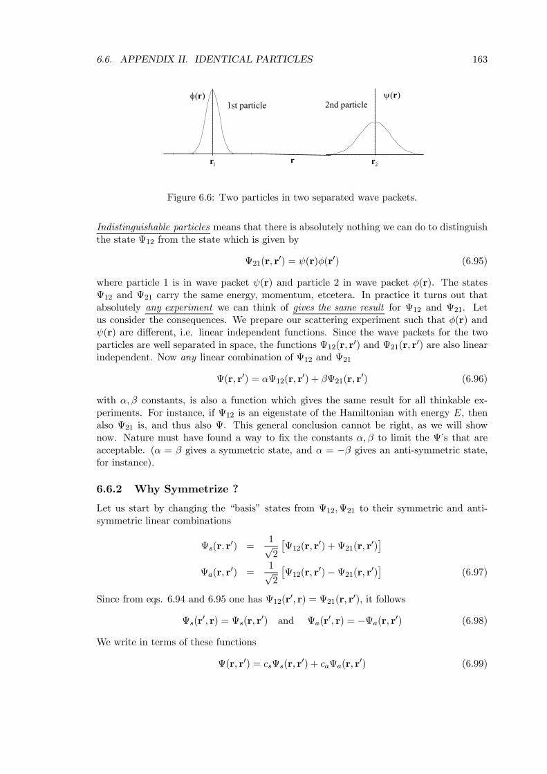
6.6. APPENDIX II. IDENTICAL PARTICLES 163
1r 2r
)(rφ )(rψ1st particle 2nd particle
r
Figure 6.6: Two particles in two separated wave packets.
Indistinguishable particles means that there is absolutely nothing we can do to distinguishthe state Ψ12 from the state which is given by
Ψ21(r, r0) = ψ(r)φ(r0) (6.95)
where particle 1 is in wave packet ψ(r) and particle 2 in wave packet φ(r). The statesΨ12 and Ψ21 carry the same energy, momentum, etcetera. In practice it turns out thatabsolutely any experiment we can think of gives the same result for Ψ12 and Ψ21. Letus consider the consequences. We prepare our scattering experiment such that φ(r) andψ(r) are different, i.e. linear independent functions. Since the wave packets for the twoparticles are well separated in space, the functions Ψ12(r, r
0) and Ψ21(r, r0) are also linearindependent. Now any linear combination of Ψ12 and Ψ21
Ψ(r, r0) = αΨ12(r, r0) + βΨ21(r, r
0) (6.96)
with α,β constants, is also a function which gives the same result for all thinkable ex-periments. For instance, if Ψ12 is an eigenstate of the Hamiltonian with energy E, thenalso Ψ21 is, and thus also Ψ. This general conclusion cannot be right, as we will shownow. Nature must have found a way to fix the constants α,β to limit the Ψ’s that areacceptable. (α = β gives a symmetric state, and α = −β gives an anti-symmetric state,for instance).
6.6.2 Why Symmetrize ?
Let us start by changing the “basis” states from Ψ12,Ψ21 to their symmetric and anti-symmetric linear combinations
Ψs(r, r0) =
1√2
£Ψ12(r, r
0) +Ψ21(r, r0)¤
Ψa(r, r0) =
1√2
£Ψ12(r, r
0)−Ψ21(r, r0)¤
(6.97)
Since from eqs. 6.94 and 6.95 one has Ψ12(r0, r) = Ψ21(r, r0), it follows
Ψs(r0, r) = Ψs(r, r0) and Ψa(r
0, r) = −Ψa(r, r0) (6.98)
We write in terms of these functions
Ψ(r, r0) = csΨs(r, r0) + caΨa(r, r0) (6.99)
164 CHAPTER 6. BOSONS AND FERMIONS
with ca and cs constants. Eq. 6.99 is just another way of writing eq. 6.96. The “basis”states Ψs and Ψa just prove to be more handy. Initially we had two separate wave packets,but now we start our scattering experiment. When the two particles start to collide, theirwave packets start to overlap. We ask for the probability of finding a particle at theposition r and a particle at the position r0 at a time t after we started the experiment.Particle 1 can be at r and particle 2 at r0, or particle 1 at r0and particle 2 at r, and thesetwo probabilities are independent. Thus the total probability is given by
P (r, r0, t) =¯Ψ(r, r0, t)
¯2+¯Ψ(r0, r, t)
¯2(6.100)
Using eqs. 6.98 and 6.99, it is easy to prove that Ψ(r0, r) = csΨs(r, r0)− caΨa(r, r0) fromwhich one finds
P (r, r0, t) = |cs|2¯Ψs(r, r
0, t)¯2+ |ca|2
¯Ψa(r, r
0, t)¯2
(6.101)
Eq. 6.101 is supposed to give the same result independent of the numbers ca and cs ! (Traceback our reasoning: since we have two indistinguishable particles, any measurement mustgive the same result for Ψ12 and Ψ21, and thus for any linear combination of the two, Ψ).If this is true then by choosing cs = 1 and ca = 0 or cs = 0 and ca = 1, it follows¯
Ψs(r, r0, t)¯=¯Ψa(r, r
0, t)¯
(6.102)
At the start of our experiment this is indeed true. We have from eq. 6.97¯Ψs(r, r
0, t)¯2=1
2 ¯Ψ12(r, r0, t)¯2 + ¯Ψ21(r, r0, t)¯2 +
Ψ∗12(r, r0, t)Ψ21(r, r0, t) +Ψ∗21(r, r
0, t)Ψ12(r, r0, t)¯Ψa(r, r
0, t)¯2=1
2 ¯Ψ12(r, r0, t)¯2 + ¯Ψ21(r, r0, t)¯2 −
Ψ∗12(r, r0, t)Ψ21(r, r0, t)−Ψ∗21(r, r0, t)Ψ12(r, r0, t) (6.103)
The Ψ12,Ψ21 cross-terms are zero at the start t = 0, because we start with well-separatedwave packets. Using eqs. 6.94 and 6.95 one gets terms like φ∗(r)φ(r0)ψ(r0)ψ∗(r) in thesecross-terms. Since φ(r) is localized around r = r1, and ψ(r) is localized around r = r2,their product φ(r)ψ(r) = 0 everywhere. fHowever, the cross-terms do not disappear whenthe wave packets start to overlap. For example, suppose the two particles collide withoutan interaction potential being present, as, for instance photons or phonons can do; thewave packets will then just pass through one another without distortion. At a certain timet1 the wave packets will overlap. This situation is pictured in Fig. 6.7.
For a point r in this overlap region, i.e. r0 = r one has Ψ12(r, r, t1) = Ψ21(r, r, t1) (seeeqs. 6.94 and 6.95), and thus from eq. 6.97
Ψs(r, r, t1) =√2Ψ12(r, r, t1) 6= 0
Ψa(r, r, t1) = 0 (6.104)
Most certainly, eq. 6.102 does not hold here ! Going back to eq. 6.101 it means that theprobability P (r, r0, t) depends on the values of ca and cs. For example, choosing cs = 1and ca = 0 or cs = 0 and ca = 1 certainly gives a very different result in view of eq.6.104. The outcome of our experiment thus depends upon ca and cs. However, we started
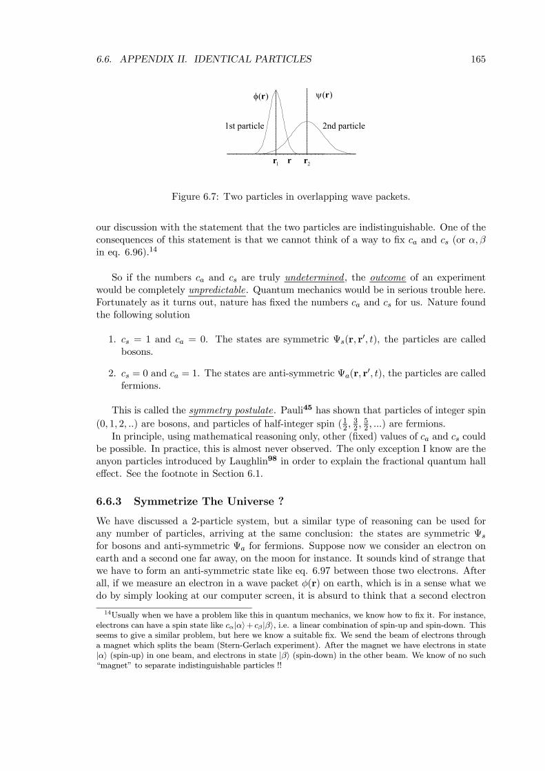
6.6. APPENDIX II. IDENTICAL PARTICLES 165
1r
)(rφ
2r
)(rψ
1st particle 2nd particle
r
Figure 6.7: Two particles in overlapping wave packets.
our discussion with the statement that the two particles are indistinguishable. One of theconsequences of this statement is that we cannot think of a way to fix ca and cs (or α,βin eq. 6.96).14
So if the numbers ca and cs are truly undetermined , the outcome of an experimentwould be completely unpredictable. Quantum mechanics would be in serious trouble here.Fortunately as it turns out, nature has fixed the numbers ca and cs for us. Nature foundthe following solution
1. cs = 1 and ca = 0. The states are symmetric Ψs(r, r0, t), the particles are called
bosons.
2. cs = 0 and ca = 1. The states are anti-symmetric Ψa(r, r0, t), the particles are called
fermions.
This is called the symmetry postulate. Pauli45 has shown that particles of integer spin
(0, 1, 2, ..) are bosons, and particles of half-integer spin (12 ,32 ,52 , ...) are fermions.
In principle, using mathematical reasoning only, other (fixed) values of ca and cs couldbe possible. In practice, this is almost never observed. The only exception I know are theanyon particles introduced by Laughlin98 in order to explain the fractional quantum halleffect. See the footnote in Section 6.1.
6.6.3 Symmetrize The Universe ?
We have discussed a 2-particle system, but a similar type of reasoning can be used forany number of particles, arriving at the same conclusion: the states are symmetric Ψsfor bosons and anti-symmetric Ψa for fermions. Suppose now we consider an electron onearth and a second one far away, on the moon for instance. It sounds kind of strange thatwe have to form an anti-symmetric state like eq. 6.97 between those two electrons. Afterall, if we measure an electron in a wave packet φ(r) on earth, which is in a sense what wedo by simply looking at our computer screen, it is absurd to think that a second electron
14Usually when we have a problem like this in quantum mechanics, we know how to fix it. For instance,electrons can have a spin state like cα|αi+ cβ |βi, i.e. a linear combination of spin-up and spin-down. Thisseems to give a similar problem, but here we know a suitable fix. We send the beam of electrons througha magnet which splits the beam (Stern-Gerlach experiment). After the magnet we have electrons in state|αi (spin-up) in one beam, and electrons in state |βi (spin-down) in the other beam. We know of no such“magnet” to separate indistinguishable particles !!
166 CHAPTER 6. BOSONS AND FERMIONS
in a wave packet ψ(r) on the moon should matter at all (unless you believe in astrology).The neat way out of this dilemma is eq. 6.103, where we have already argued that in casethe two wave packets do not overlap we get¯
Ψa(r, r0, t)¯2
=1
2
n¯Ψ12(r, r
0, t)¯2+¯Ψ21(r, r
0, t)¯2o
=1
2
n|φ(r, t)|2 |ψ(r0, t)|2 + |ψ(r, t)|2 |φ(r0, t)|2
o(6.105)
Note that if r is on earth, the second term in eq. 6.105 gives zero, because obviously the“moon” wave packet ψ(r) = 0 for points on earth. The probability distribution of eq.6.100 gives
P (r, r0, t) =¯Ψa(r, r
0, t)¯2+¯Ψa(r
0, r, t)¯2
= |φ(r, t)|2 |ψ(r0, t)|2 (6.106)
which means that the probability distribution for the “earth” electron is given by |φ(r, t)|2 ,independent of that of the “moon” electron |ψ(r0, t)|2, as common sense demands. If wedo a position measurement of the “earth” electron we get the expectation value
hΨa|r|Ψai =
Z ZrP (r, r0, t) d3r d3r0 =
Z Zr |φ(r, t)|2 |ψ(r0, t)|2 d3r d3r0
=
Zr |φ(r, t)|2 d3r ·
Z|ψ(r0, t)|2d3r0 =
Zr |φ(r, t)|2 d3r (6.107)
So indeed the “moon” electron does not have any influence on this measurement. The anti-symmetric state Ψa of the “earth-moon” electron pair does not produce something whichcontradicts common sense, which is reassuring. However it still seems a bit “overdone”.Note that the probability distribution of eq. 6.106 is identical to
P (r, r0, t) = |Ψ12(r, r0, t)|2
This means that for two electrons so far apart that their wave functions do not overlap,we can assume that electron 1 is “here” (i.e. around r = r1) and electron 2 is “there” (i.e.around r = r1). In other words we can pretend that we can distinguish the two electronsfrom one another. Making them indistinguishable by anti-symmetrizing their total wavefunction is not wrong, but it produces the same distribution. Note that the same reasoningdoes not hold anymore if the cross terms in eq. eq. 6.103 cannot be neglected. This isthe case if the wave packets of the two electrons overlap. The probability distribution ofthe two electrons cannot be written anymore as a product of two distribution in whichone only involves the first electron and the other only the second electron. If this is thecase then measuments on one electron cannot be independent of the second electron, andone has to use the full distribution P (r, r0, t). The two electrons are then called entangled,and the anti-symmetric wave function is an example of an entangled state (i.e. one thatcannot be written as a simple product).15
15Entangled states play a key role in fundamental discussions on quantum mechan-ics involving the famous Einstein-Podolsky-Rosen (EPR) paradox, for instance. Seehttp://www.nobel.se/physics/educational/tools/theoretical.html, and modern quantum mechanicsbooks such as D. J. Griffith, Introduction to Quantum Mechanics, (Prentice Hall, Upper Saddle River,1995); or R. I. Liboff, Introductory Quantum Mechanics, (Addison Wesley, Reading, 1997).Entangled states also play an essential role in modern research on “quantum computing”.
6.6. APPENDIX II. IDENTICAL PARTICLES 167
Finally, for those of you who wonder whether it is necessary to include all electrons inthe universe in an anti-symmetric wave function, you may; it is not wrong, but it wouldbe overdone. If you only anti-symmetrize the wave function of the entangled electrons, i.e.the ones that are close to one another, such that their wave packets overlap, and pretendthat you can distinguish them from those in the rest of the universe, you get the correctresults. Needless to say that, although the discussion has been for electrons, it also holdsfor any kind of fermion or boson (using symmetric states in the latter case, of course).

168 CHAPTER 6. BOSONS AND FERMIONS
Chapter 7
Optics
“Macht doch den zweiten Fensterladen auch auf, damit mehr Licht hereinkomme”, Goethe’s dying
words (“Please open also the second shutter, so more light can come in”).
In the previous two chapters we have looked at “pure” fermion or boson systems of non-interacting particles. Most of the interesting physics happens of course when particles areinteracting with each other. In this chapter we will look at an “enlightening” example offermions interacting with bosons, namely electrons interacting with photons, which givesrise to all familiar optical processes. Second quantization presents a unified approach fordescribing systems of fermions, such as electrons, systems of bosons, such as photons, aswell as the coupling between such systems.1 So, although we are focusing on optics inthis chapter, the general strategy is also applicable to other fermion and boson systems.We start by reviewing some of the optics we discussed in Chapter 2, but now from a fullyquantum mechanical point of view in which everything, radiation as well as matter, isdescribed in terms of quantum states and operators. The first part descibes atoms in EMfields as in Section 2.4. As we shall see, a full quantum mechanical approach allows us tosolve some of the problems we encountered in the semi-classical approach of Chapter 2, seeSection 2.5. In the second part we will consider optical processes in many-fermion systems,using the homogeneous electron gas of Section 6.3.1. We will introduce Feynman diagramsfor interacting electrons, holes and photons, and discuss their connection to perturbationtheory. In the first appendix the Hamiltonian of an electron in an EM field is derived.This chapter more or less rounds up the description of non-relativistic quantum electro-dynamics. A few aspects of relativistic electrons and holes (positrons) are discussed in thesecond appendix.
7.1 Atoms and Radiation; the Full Monty
In stone-age notation the Hamiltonian of an atom having N electrons is given by
bHatom = bh+ bv = NXi=1
· bp2i2m
+−Ze2|bri|
¸+1
2
NXi6=j
e2
|bri − brj | (7.1)
1I use the phrase “second quantization”. You might also use the phrase “number representation”, or(if you aspire to be an elementary particle physicist) “quantum fields”. In the present context they are allsynonyms.
169
170 CHAPTER 7. OPTICS
see Section 6.1.3. The first sum at the right hand side is a one-particle operator whichgives the kinetic energy of the electrons and their Coulomb interaction with the nucleus.The second sum is a two-particle operator which gives the Coulomb repulsion betweenthe electrons. We assume that the nucleus is at a fixed position at the origin (so R = 0in comparison to Section 6.1.3). Furthermore we have defined a convenient (orthonormaland complete) basis set |ki of atomic orbitals, which allows us to rewrite the atomicHamiltonian in second quantized form
bHatom =Xk,l
hklbc†kbcl + 12 Xk,l,m,n
vklmnbc†lbc†kbcmbcn (7.2)
according to eqs. 6.34 and 6.35 in Section 6.2.2. The operators bc†k,bck create, annihilatean electron in a state |ki of the basis set. Obviously these are fermion operators, so theyanti-commutate. The Hamiltonian bHatom provides a complete description of the atom.
The Hamiltonian which describes the EM radiation field (in vacuum) is
bHrad =XK,s
½ba†K,sbaK,s + 12¾~ωK (7.3)
=XK,s
~ωKba†K,sbaK,s +E0according to eq. 5.79 in Section 5.5, where we have used eq. 6.44 to convert to a discreteset of states, normalized in a box of volume Ω. E0 is the energy of the photon vacuumstate, which can be treated as an unspecified constant. The operators ba†K,s,baK,s create,annihilate a photon of momentum ~K and polarization s. These are boson operators, sothey commutate. The Hamiltonian bHrad provides a complete description of the radiationfield in vacuum. Since electrons and photons clearly are distinguishable, a basic quantumstate for the complete system atom+radiation can be expressed as a product, see Section1.4
|Ψi = |ψatomi|φradi (7.4)
The “full” Hamiltonian operates on this state as
bH0 = bHatom + bHradbH0|Ψi =³ bHatom|ψatomi´ |φradi+ |ψatomi³ bHrad|φradi´ (7.5)
Perhaps one is inclined to think that the description is now complete.
However, the atom and the radiation field interact. According to Section 2.4 thisinteraction is represented by the operator
bV = −bµ · bE = e NXi=1
bri · bE (7.6)
in stone-age notation, cf. eqs. 2.41 and 2.42 (note we have set R = 0 again). In Section2.4 we used in this expression quantum operators bri for the electrons, in combination with
7.1. ATOMS AND RADIATION; THE FULL MONTY 171
a classical electric field E, which made the operator bV semi-classical. Now we assume thatbV is a fully quantum mechanical operator in which also the electric field is an operatorbE according to Section 5.5. We don’t have a stone-age representation for bE, since firstquantization or wave functions do not exist for photons, so to be consistent we musttransform eq. 7.6 into a full second quantized form. Since bri and bE operate on differentsubsystems (electrons and photons, respectively), we may consider them one at a time.The electronic part is a one-particle operator and its second quantized form is given by
NXi=1
bri → Xk,l
rklbc†kbcl with
rkl = hk(1)|r1|l(1)i (7.7)
according to eq. 6.34. The electric field is given by
bE(r, t) = −∂ bA∂t
= −iµ
~2ε0Ω
¶12 XK,s
√ωK
³baK,se−iωKt − ba†−K,seiωKt´ εK,seiK·r (7.8)
according to eqs. 5.71 and 5.72 in Section 5.5, where we have used the “discretization”trick of eq. 6.44 again. In order to be consistent this expression has to be modifiedslightly. All atomic operators are time independent, cf. eqs. 7.2 and 7.7, which meansthat we use the Schrodinger picture. The time dependence in the electric field resultsfrom the Heisenberg picture; to convert it into the Schrodinger picture, we set t = 0, cf.eq. 2.64 in Section 2.6. Furthermore, in deriving eqs. 2.41 and 2.42 (and thus eq. 7.7)we have assumed that the electric field is homogeneous, i.e. spatially independent. Thiswas justified by the fact that the wave length of EM radiation is much larger than thesize of the atom, see Section 2.4. For obvious reasons this is called the long wave lengthapproximation. The electric field operator now becomes2
bE = −iµ ~2ε0Ω
¶ 12 XK,s
√ωK
³baK,s − ba†−K,s´ εK,s (7.9)
Using eqs. 7.7 and 7.9 in eq. 7.6 gives for the interaction operator
bV =XK,s;k,l
βK,s;k,l
³baK,sbc†kbcl − ba†−K,sbc†kbcl´ with (7.10)
βK,s;k,l = −ieµ~ωK2ε0Ω
¶ 12
εK,s · rkl
This operator describes the coupling or interaction between the atom and the radiationfield. According to the reasoning below eq. 6.38 in Section 6.2.3, the first term betweenbrackets in eq. 7.10 describes the annihilation of an electron in state l, accompanied by theannihilation of a photon in state K,s and the creation of an electron in state k. In otherwords it describes the excitation from l to k by absorption of a photon. The correspondingdiagram is given in Fig. 6.3. In a similar way, the second term between brackets in eq.
2Note that since the electric field is an observable, it must be an Hermitian operator, i.e. bE† = bE, fromwhich it follows that εK,s = ε−K,s. (We already know that ωK = c|K| = ω−K).
172 CHAPTER 7. OPTICS
7.10 descibes the de-excitation from l to k and emission of a photon. It can be representedby a similar diagram with the arrow on the photon line reversed.
The Hamiltonian bH = bH0+ bV , eqs. 7.2, 7.3 and 7.10, gives a complete desciption of thesystem, atom plus radiation field. It allows us to descibe all possible optical experiments;absorption, emission, scattering of light, non-linear optics; you name it. As before, ourstrategy is to use bH0 for constructing unperturbed states, use bV as the perurbation, andthe tools of perturbation theory to study optical transitions.
MODEL; A TWO-LEVEL HYDROGEN ATOM
As a demonstration of how the procedure works, we reconsider the hydrogen atom ofSection 2.4 again.3 Because hydrogen contains only one electron, the atomic Hamiltoniancan be simplified. There are no other electrons present and we can neglect the two-particleterms in eq. 7.2.4 As a basis set we choose the eigenstates of the hydrogen atom, whichmakes the one-particle term in eq. 7.2 diagonal, i.e. hkl = δkl²k, and
bHhydrogen =Xk
²kbc†kbckwhere k = (n, l,m) represents the set of quantum numbers needed to fix the eigenstatesof the hydrogen atom, and ²k = ²nlm = −13.606
n2eV are the familiar energy levels of the
hydrogen atom. We simplify the discussion even further by selecting just two of thesestates, the 1s state, which we call |ii, and the 2px state, which we call |fi. The simplifiedHamiltonian becomes
bHhydrogen → bh = ²ibc†ibci + ²fbc†fbcf (7.11)
where ²i = ²1s = −13.606 eV, and ²i = ²2px = −3.402 eV. The two-state basis set |ii and|fi also allows us to simplify eq. 7.7 to
rifbc†ibcf + rfibc†fbci with (7.12)
rif = h1s|r|2pxi
and the atom-field interaction of eq. 7.7 is then simplified to
bV =XK,s
βK,s;if
³baK,sbc†ibcf − ba†−K,sbc†ibcf´+βK,s;fi
³baK,sbc†fbci − ba†−K,sbc†fbci´ (7.13)
3The hydrogen atom is chosen for convenience, since it simplifies the calculations. The method isgenerally applicable to atoms and molecules. For solid state materials, see the second part of this chapter.
4The two-particle term contains two annihilation operators; working on a one-particle state, it alwaysgives zero. In principle EM radiation can create other electrons (and positrons), which could interact withthe one electron in the hydrogen atom. However, this process happens only at a very high energy; weneglect it here.
7.1. ATOMS AND RADIATION; THE FULL MONTY 173
7.1.1 Absorption; Fermi’s Golden Rule
Now let us do the following experiment. We prepare the atom in the 1s state, and theradiation field in a state in which there is one photon present with momentum ~Q andpolarization along the x-axis, i.e. εQ,s = ex. So the complete initial state is given insecond quantization notation by
|Ψinii = |ψini,atomi|φini,radi = |1ii|1Q,xi ≡ |1i; 1Q,xi (7.14)
We are interested in a final state in which the atom is in the 2px state and the radiationfield is in its ground state, i.e. no photons present.
|Ψfini = |ψf,atomi|φf,radi = |1f i|0i ≡ |1f ; 0i (7.15)
We wish to calculate the transition amplitude between initial and final statesDΨfin|bU(t, t0)|ΨiniE ; t > t0 where (7.16)
bU(t, t0) = e−i~ (t−t0) bH and bH = bh+ bHrad + bV
As in Section 2.3 we first consider the Born approximation, which neglects all terms beyondfirst order perturbation
bU(t, t0) ≈ bU0 (t, t0) + bU (1) (t, t0) (7.17)
= bU0 (t, t0) + 1
i~
Z t
t0
dτ bU0 (t, τ) bV bU0 (τ , t0)where bU0(t, t0) = e−
i~ (t−t0) bH0 and bH0 = bh+ bHrad
We follow exactly the same procedure as outlined in Section 2.3. According to eqs. 7.3,7.5 and 7.11, we have
bH0|Ψinii =³bh|1ii´ |1Q,xi+ |1ii³ bHrad|1Q,xi´
= (²i + ~ωQ +E0)|Ψinii (7.18)
and in a similar way
bH0|Ψfini = (²f +E0)|Ψfini (7.19)
Therefore DΨfin|bU0(t, t0)|ΨiniE = e− i
~ (t−t0)(²i+~ωQ+E0)hΨfin|Ψinii = 0
since the states are orthogonal. The zero’th order term of eq. 7.17 gives no contributionin eq. 7.16. Working out the first order term as in Section 2.3 givesD
Ψfin
¯ bU (t, t0)¯ΨiniE =1
i~
Z t
t0
dτ e−i~ (t−τ)(²f+E0) Vfin,ini e−
i~ (τ−t0)(²i+~ωQ+E0)
with Vfin,ini = hΨfin|bV |Ψinii (7.20)
174 CHAPTER 7. OPTICS
The integral can be done, which yields the transition rate
wini→fin =d
dt
¯DΨfin
¯ bU (t, t0)¯ΨiniE¯2 = 2π
~2|Vfin,ini|2 δ (ωfi − ωQ) (7.21)
where ωfi = (²f − ²i)/~
under the same conditions as discussed in Section 2.3.
This is Fermi’s golden rule again, cf. eq. 2.32. It will lead to a similar expressionas eq. 2.45 in Section 2.4 for the transition in the hydrogen atom. However, notice thedifferences with our earlier derivation
• The EM field is not treated as an external semi-classical perturbation, but it is partof the quantum description now. The “perturbation” is the coupling bV between theatom and the radiation field, eq. 7.13.
• The perturbation operator has no time dependence (which according to Schrodingeris the correct procedure). All time dependence is in the time evolution operatorbU (t, t0), eq. 7.17.
• The δ-function in eq. 7.21 now truly describes the conservation of energy, ²i+~ωQ =²f ; i.e. transitions are only allowed between states |Ψinii and |Ψfini which have thesame energy, cf. eqs. 7.18 and 7.19.
What remains is the calculation of the matrix element Vfin,ini.
Vfin,ini = hΨfin|bV |Ψinii= h1f ; 0|
XK,s
βK,s;if
³baK,sbc†ibcf − ba†−K,sbc†ibcf´+βK,s;fi
³baK,sbc†fbci − ba†−K,sbc†fbci´ |1i; 1Q,xi= h1f ; 0|βQ,x;fibaQ,xbc†fbci|1i; 1Q,xi= βQ,x;fi = −ie
µ~ωQ2ε0Ω
¶12
ex · rfi (7.22)
It is easy to see that only the third term of the right hand side of eq. 7.13 is contributingto this matrix element. The first two terms contain bcf , and try to annihilate a particle instate |fi, which is not present. The fourth term creates a photon, instead of annihilatingone. Of the sum over K,s only the one Q,x term yields a non-zero contribution to Vfin,ini,since all the photon states of the radiation field are orthogonal (work it out yourself).Since ex · rfi = xfi = hf |bx|ii, according to eq. 7.12, we get
|Vfin,ini|2 = |βQ,x;fi|2 =e2~ωQ2ε0Ω
|hf |bx|ii|2 (7.23)
which gives for the transition rate of eq. 7.21
wini→fin =πe2~ωQ~2ε0Ω
|hf |bx|ii|2 δ (ωfi − ωQ) (7.24)
7.1. ATOMS AND RADIATION; THE FULL MONTY 175
The term~ωQΩ is the excess energy density that is present in the radiation field (i.e. energy
on top of the vacuum energy) at the start of our “experiment”, since we started with onephoton of energy ~ωQ in a volume Ω. It is not difficult to show that if we start withnQ photons in this mode, a similar calculation shows that the transition rate simply isproportional to nQ. For a classical electric field E = E0 cosωt as we used in Section2.4, the energy density is 1
2ε0E20 . This means that eq. 7.24 corresponds exactly to the
semi-classical result we found before, cf. eq. 2.45. So all the physical concepts we haveintroduced in Section 2.4, oscillator strengths, selection rules, Einstein coefficients, remainvalid.
7.1.2 Spontaneous Emission
However we can do much more than just recovering the results of Section 2.4. For instancewe can calculate the probability amplitudeD
Ψfin|bU(t, t0)|ΨfinE (7.25)
where we have prepared at time t0 our atom in the excited state |fi with no photonspresent, and probe the probability that is still in this state at a later time t. In otherwords, we are interested in the decay of the excited state. We can do a full calculation,but in this case we already know in general terms what the outcome will be. Although thephysics is a little bit different, mathematically this problem looks like the problem we havesolved in Chapter 4, compare eq. 7.25 to eq. 4.20. Just like in that chapter we can sumthe complete perturbation series in bV (including all orders), by using the self-energy Σ.Without going through all the algebra for this particular case, we know from the resultsof Chapter 4 that the general result according to eq. 4.39 is5D
Ψfin|bU(t, t0)|ΨfinE = e− i~ [²f+∆f ](t−t0)e−
12Γf (t−t0) for t > t0 (7.26)
where the level shift ∆f and the decay constant Γf are related to the self-energy Σ ac-cording to eq. 4.38.6 The probability that the atom is in its excited state is given by
Nf (t) =¯DΨfin|bU(t, t0)|ΨfinE¯2 = e−Γf (t−t0) (7.27)
The occupancy of the excited state (which is just another word for this probability) isdecaying exponentially. In this case the decay rate Γf can even be obtained analyticallyfrom the self-energy. Assume that we can do the algebra, and observe that eq. 7.27corresponds exactly to eq. 2.59 in Section 2.4, because we started from an occupancyNf (t0) = 1. In other words, we have recovered the Einstein rate equation and thereforewe have found
Γf = Afi (7.28)
5A famous quote of Feynman is “...the same equations have the same solutions...”. It means that, ifyou have two equations which look similar, although they may come from completely different fields inphysics, the solutions also must have a similar form. It sounds trivial, but it is a much used principle inphysics. The strive towards “unification theories” stems from the desire to make different equations look“similar”.
6The weight factor zf = 1 for the same reason as in eq. 4.38, namelyDΨfin|bU(t0, t0)|Ψfin
E=
hΨfin|Ψfini = 1.
176 CHAPTER 7. OPTICS
which is the Einstein coefficient for spontaneous decay, cf. eq. 2.60. But we have obtainedit now from quantum mechanical first principles, without needing a phenomenologicalmodel!! Our state |Ψfini has no photons to start with, but the perturbation bV of eq. 7.13couples it to other states, which leads to a probability that the atom emits a photon andfalls to a lower atomic level. Since this occurs without the need for an external field, i.e.in the radiation field vacuum, this process is truly spontaneous and cannot be switchedoff.
We have solved some of the problems mentioned in Section 2.5 by our fully quantummechanical approach. The complete Einstein equations can also be derived; it is possibleto calculate the Compton scattering of Section 5.5.3 by this approach, or any other opticalprocess you might be interested in.7
In addition to a decay, eq. 7.27 also predicts that the atomic level ²f is shifted to ²f+∆fby the coupling of the atom to the radiation field. Calculating the shift ∆f involves somesubttleties which I won’t discuss now, but it can be done. What is more important, theshift can be measured experimentally, and theory and experiment agree. From elementaryquantum mechanics we obtained the energy levels of the isolated hydrogen atom, butnow we see that coupling with the radiation field vacuum states shifts these levels.8 Theshifts are small, i.e. ∼ 109Hz (which is at the ppm level for hydrogen levels), but theycan be measured! The prediction of these shifts is considered to be one of the greatsuccesses of quantum electrodynamics. To be fair, there are also shifts due to relativisticeffects. The “speed” of the electron can no longer be neglected as compared to the speedof light if one is interested in such small level shifts. Relativistic shifts are an order ofmagnitude larger than the shifts due to the coupling with the radiation field, but they canalso be calculated, by using the relativistic Dirac equation instead of the non-relativisticSchrodinger equation for the hydrogen atom. The relativistic theory lifts some of thedegeneracies that are present in the non-relativistic spectrum of the hydrogen atom, bute.g. the 2s 1
2and 2p 1
2levels are still degenerate.9 Coupling to the radiation field splits
these levels, and the resulting splitting of ∼ 109Hz, which is called the Lamb shift, can bemeasured.
7.2 Electrons, Holes and Photons
“What is the use of a book, thought Alice, without pictures or conversations”, Lewis Caroll, Alice’s
Adventures in Wonderland.
In this section we will consider optical processes related to “free” electrons, using thehomogeneous electron gas of Section 6.3.1. Feynman diagrams are introduced that describeprocesses involving electrons, holes and photons, and their connection to perturbationtheory is discussed.
7If you are interested, see C. Cohen-Tannoudji, J. Dupont-Roc, and G. Grynberg, Atom-Photon Inter-actions, (Wiley, New York, 1998).
8Again I want to stress that this is a “spontaneous” effect, i.e. it exists in vacuum. All it requires isthe coupling operator of eq. 7.10, not an external field!
9See B. H. Brandsen and C. J. Joachain, Quantum Mechanics, (Prentice-Hall, Harlow, 2000), Ch. 8and 15.
7.2. ELECTRONS, HOLES AND PHOTONS 177
7.2.1 Electrons and Radiation
The hamiltonian bh of a homogeneous “free” electron gas is given by eq. 6.51.bh =Xk
²kbc†kbck= E0,el −
X|k|≤kF
²kbb†kbbk + X|k|>kF
²kba†kbak (7.29)
with ²k =~2 |k|22m
(7.30)
where bc†k b, ck refer to general fermion creation, annihilation operators and ba†k,bak and bb†k,bbkrefer to the particle and hole operators introduced in Section 6.3.1. E0,el is the energy ofthe ground state (vacuum) of the electron gas; we do not need to calculate it explicitly.The Hamiltonian bHrad of a “free” radiation field is still given by eq. 7.3. bH0 = bh+ bHradis an “unperturbed” Hamiltonian like the one in eq. 7.5. Again, a perturbation bV whichcouples the electronic system to the radiation field needs to be constructed as in theprevious section. However, eq. 7.6 is no good here! That equation was derived assumingthe long wave length limit, i.e. the wave length of the EM radiation is much larger thanthe “size” of the electronic system, see also Section 2.4. This is reasonable for a smallatom, but not for a free electron. The latter has an infinite extension, or, if we use statesthat are normalized in a box, the electronic wave functions have the same extension as theEM waves. The correct expression which describes the interaction between the electronicand the photonic system is given by10
bV = e
m
NXj=1
bA(brj) · bpj (7.31)
in stone-age representation, where bpi is the momentum operator of the i’th electron andbA(bri) is the vector potential. A derivation of this expression is given in Appendix I. Thevector potential operator is given by
bA(br) =1√Ω
XK,s
bqK,sεK,seiK·br (7.32)
bqK,s =
µ~
2ε0ωK
¶ 12 ³baK,s + ba†−K,s´
according to eq. 5.72 in Section 5.5, where we have switched to a “discrete” set of statesagain using eq. 6.44, and we have set t = 0, because we wish to work in the Schrodingerrepresentation. Note that the spatial dependent part eiK·br is considered to be an operatorin electron space!
The expression for the interaction we used in the atomic case, cf. eq. 7.6, looks quite a bitdifferent from eq. 7.31. However, the “atomic” expression can be derived from the latter,
10Electrons also carry a spin sj , which has an interaction with the magnetic field. This contributes aterm gee
2m
PNj=1 bsj · bB(brj) to the interaction. This term is usually small, and we neglect it here. See also
the footnote in Section 6.3.1.
178 CHAPTER 7. OPTICS
which is also shown in Appendix I. The “atomic” expression of eq. 7.6 only works in thelong wave length limit, i.e. when the spatial dependence of the fields may be neglected.This is valid for small systems like atoms, but in other cases the more general form of eq.7.31 has to be used.
As in the previous section, the only way to make progress is to transform eq. 7.31 into asecond quantized expression. Since we are dealing with the homogeneous electron gas, weuse its eigenstates as the basis set for our electronic system, see eqs. 6.40—6.42 in Section6.3.1. Proceeding as for eq. 7.7, we obtain the second quantized form of the spatiallydependent part of eq. 7.31
NXj=1
eiK·brjbpj →Xk,l
πklbc†kbcl with
πkl = hk|eiK·brbp|li = 1
Ω
ZΩd3r e−ik·reiK·r
~i∇eil·r
~lΩ
ZΩd3r ei(K−k+l)·r = ~lδk−K,l (7.33)
where we have used eq. 6.41 (see also Chapter 4, eq. 4.17). Using eqs. 7.32 and 7.33 ineq. 7.31 gives the required second quantized form for the interaction operatorbV = X
K,s;l
γK,s;l
³baK,sbc†l+Kbcl + ba†−K,sbc†l+Kbcl´ (7.34)
with γK,s;l =e
m
µ~
2ε0ΩωK
¶ 12
~l · εK,s
As before, the terms in eq. 7.34 have a physical meaning. The first term describesabsorption of a photon of momentum ~K and polarization s, accompanied by an excitationof an electron with momentum ~l to momentum ~(l+K); the second term describes anemission process. We can convert this operator according to the particle-hole formalismby making the substitutions bcl = bal if ²l > ²F and bcl = bb†l if ²l ≤ ²F . Note that if ²l ≤ ²F , itis possible that ²l+K > ²F , if K is large enough (and positive). So the coupling bV containsparticle-hole terms, as well as particle-particle and hole-hole terms.11bV =
XK,s;|l|>kF ,|l+K|>kF
γK,s;l
³baK,s + ba†−K,s´ba†l+Kbal (7.35)
+X
K,s;|l|≤kF ,|l+K|>kFγK,s;l
³baK,s + ba†−K,s´ba†l+Kbb†l (7.36)
+X
K,s;|l|≤kF ,|l+K|≤kFγK,s;l
³baK,s + ba†−K,s´bbl+Kbb†l (7.37)
+X
K,s;|l|>kF ,|l+K|≤kFγK,s;l
³baK,s + ba†−K,s´bbl+Kbal (7.38)
11The notation becomes a bit messy, but I will use the “K,s” subscript for photon operators ba†K,s,baK,s(with boson commutation rules) and the “k” subscript for electron operators ba†k,bak (with fermion anti-commutation rules).
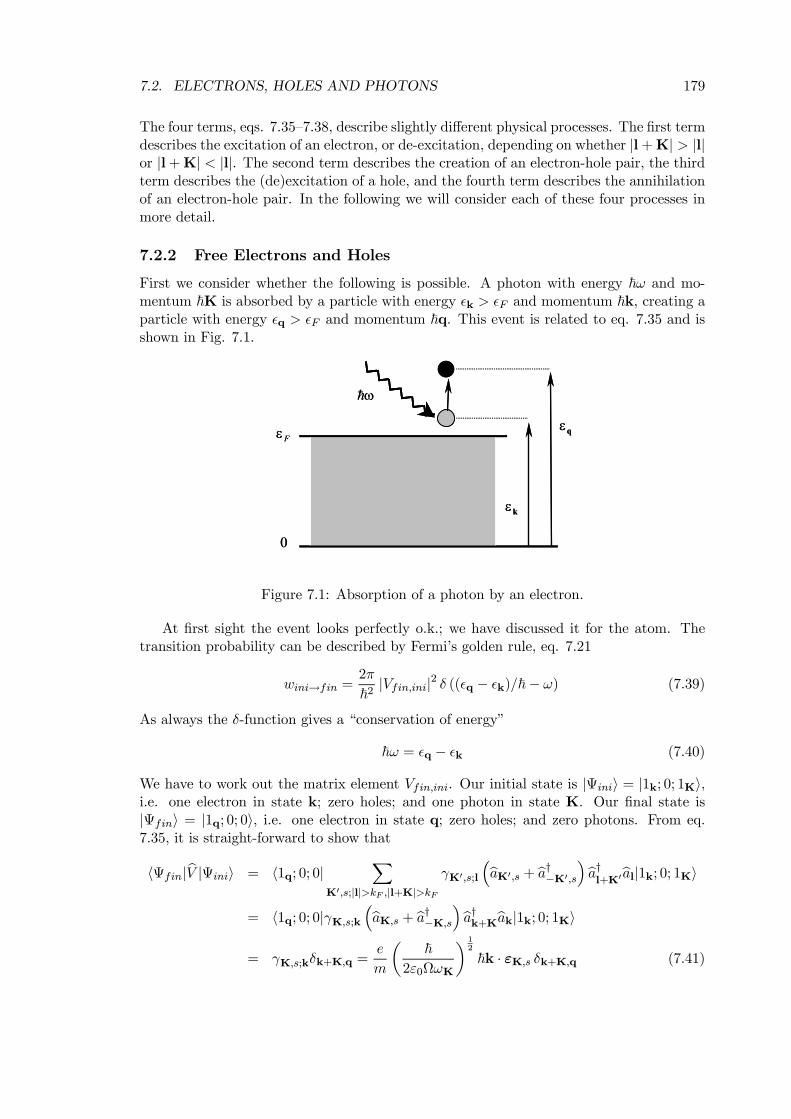
7.2. ELECTRONS, HOLES AND PHOTONS 179
The four terms, eqs. 7.35—7.38, describe slightly different physical processes. The first termdescribes the excitation of an electron, or de-excitation, depending on whether |l+K| > |l|or |l+K| < |l|. The second term describes the creation of an electron-hole pair, the thirdterm describes the (de)excitation of a hole, and the fourth term describes the annihilationof an electron-hole pair. In the following we will consider each of these four processes inmore detail.
7.2.2 Free Electrons and Holes
First we consider whether the following is possible. A photon with energy ~ω and mo-mentum ~K is absorbed by a particle with energy ²k > ²F and momentum ~k, creating aparticle with energy ²q > ²F and momentum ~q. This event is related to eq. 7.35 and isshown in Fig. 7.1.
Fε
0
εk
εq
ω
Fε
0
εk
εq
ω
Figure 7.1: Absorption of a photon by an electron.
At first sight the event looks perfectly o.k.; we have discussed it for the atom. Thetransition probability can be described by Fermi’s golden rule, eq. 7.21
wini→fin =2π
~2|Vfin,ini|2 δ ((²q − ²k)/~− ω) (7.39)
As always the δ-function gives a “conservation of energy”
~ω = ²q − ²k (7.40)
We have to work out the matrix element Vfin,ini. Our initial state is |Ψinii = |1k; 0; 1Ki,i.e. one electron in state k; zero holes; and one photon in state K. Our final state is|Ψfini = |1q; 0; 0i, i.e. one electron in state q; zero holes; and zero photons. From eq.7.35, it is straight-forward to show that
hΨfin|bV |Ψinii = h1q; 0; 0|X
K0,s;|l|>kF ,|l+K|>kFγK0,s;l
³baK0,s + ba†−K0,s
´ba†l+K0bal|1k; 0; 1Ki
= h1q; 0; 0|γK,s;k³baK,s + ba†−K,s´ba†k+Kbak|1k; 0; 1Ki
= γK,s;kδk+K,q =e
m
µ~
2ε0ΩωK
¶ 12
~k · εK,s δk+K,q (7.41)
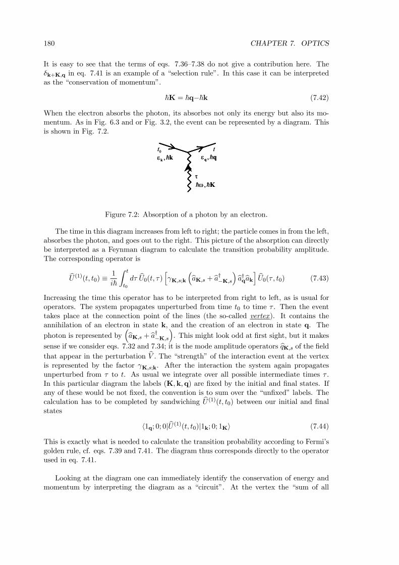
180 CHAPTER 7. OPTICS
It is easy to see that the terms of eqs. 7.36—7.38 do not give a contribution here. Theδk+K,q in eq. 7.41 is an example of a “selection rule”. In this case it can be interpretedas the “conservation of momentum”.
~K = ~q−~k (7.42)
When the electron absorbs the photon, its absorbes not only its energy but also its mo-mentum. As in Fig. 6.3 and or Fig. 3.2, the event can be represented by a diagram. Thisis shown in Fig. 7.2.
,ω K
,εk k ,εq q
τ
0t t
,ω K
,εk k ,εq q
τ
0t t
Figure 7.2: Absorption of a photon by an electron.
The time in this diagram increases from left to right; the particle comes in from the left,absorbes the photon, and goes out to the right. This picture of the absorption can directlybe interpreted as a Feynman diagram to calculate the transition probability amplitude.The corresponding operator is
bU (1)(t, t0) ≡ 1
i~
Z t
t0
dτ bU0(t, τ) hγK,s;k ³baK,s + ba†−K,s´ba†qbaki bU0(τ , t0) (7.43)
Increasing the time this operator has to be interpreted from right to left, as is usual foroperators. The system propagates unperturbed from time t0 to time τ . Then the eventtakes place at the connection point of the lines (the so-called vertex). It contains theannihilation of an electron in state k, and the creation of an electron in state q. The
photon is represented by³baK,s + ba†−K,s´. This might look odd at first sight, but it makes
sense if we consider eqs. 7.32 and 7.34; it is the mode amplitude operators bqK,s of the fieldthat appear in the perturbation bV . The “strength” of the interaction event at the vertexis represented by the factor γK,s;k. After the interaction the system again propagatesunperturbed from τ to t. As usual we integrate over all possible intermediate times τ .In this particular diagram the labels (K,k,q) are fixed by the initial and final states. Ifany of these would be not fixed, the convention is to sum over the “unfixed” labels. Thecalculation has to be completed by sandwiching bU (1)(t, t0) between our initial and finalstates
h1q; 0; 0|bU (1)(t, t0)|1k; 0; 1Ki (7.44)
This is exactly what is needed to calculate the transition probability according to Fermi’sgolden rule, cf. eqs. 7.39 and 7.41. The diagram thus corresponds directly to the operatorused in eq. 7.41.
Looking at the diagram one can immediately identify the conservation of energy andmomentum by interpreting the diagram as a “circuit”. At the vertex the “sum of all
7.2. ELECTRONS, HOLES AND PHOTONS 181
incoming arrows” must be equal to the “sum of all outgoing arrows”, like the currents inan electric circuit. This leads to ~ω+²k = ²q and ~K+ ~k =~q, which are the conservationlaws of eqs. 7.40 and 7.42. Note the fact that ²q > ²k according to our original assumption,cf. Fig. 7.1, fixes the direction of the arrow on the photon line. It means that only thebaK,s part of the photon operator in eq. 7.43 participates (i.e. the excitation from k to
q is accompanied by absorption, and not by emission). If ²q < ²k then the ba†−K,s partwould be active, which corresponds to emission. The arrow on the photon line would bereversed, and the circuit rules would give ²k = ²q− ~ω and ~k =~q+~K, which is correctfor emission.
IMPORTANT REMARK
However perfect it looks, the event is in fact forbidden. A free electron cannot absorb aphoton! The reason lies in the fact that the selection rules of eqs. 7.40 and 7.42 cannotbe obeyed simultaneously . An electron wave with a typical energy of 10 eV has a wave
length λ ≈ 4 A (and thus k = 2πλ ≈ 1.6A−1), as is easily derived from eq. 7.30. A photon
wave with an energy of 10 eV has a wave length λ ≈ 1240 A (and thus k ≈ 5× 10⁻³A−1),cf. eqs. 5.64 or 6.56. There is no way that the tiny photon momentum can supply thelarge change in the electron momentum, which is required by eq. 7.42, when at the sametime all the photon energy has to be absorbed by the electron, as required by eq. 7.40.12
The reason absorption worked for an “atomic” electron as discussed in the first partof this chapter, is because an electron that is bound in an atom is not in a momentumeigenstate, and therefore eq. 7.42 does not hold. The energy is still conserved, cf. eq.7.21. The photon momentum is absorbed by the atom as a whole (which is the microscopicorigin of “radiation pressure”). It is possible for a free electron to scatter a photon, whichis the Compton scattering discussed in Section 5.5.3. To obey the conservation rules of eq.5.82, the electron only absorbs part of the energy and momentum of the incoming photon,the rest is given to the outgoing photon.
The foregoing discussion does not depend upon whether the initial state of the particleis above or below the Fermi energy, i.e. whether ²k > ²F or ²k ≤ ²F . Suppose the latteris the case. Then absorption of a photon would create an empty state below and a filledstate above the Fermi level. This forbidden process is shown in Fig. 7.3.
Another way of looking at this process is to say that the photon of energy ~ω andmomentum ~K is annihilated and two “particles” are created. One is a particle (electron)with energy ²q and momentum ~q and the other is an anti-particle (hole) with energy −²kand momentum −~k, cf. Table 6.2. In order to see that this process is forbidden one canagain look at the conservation of energy and momentum.
~ω = ²q + (−²k)~K = ~q+ (−~k) (7.45)
12The only way to satisfy eqs. 7.40 and 7.42 simultaneously is to use high energy (small wave length,large momentum) photons. However, this would give the electron a relativistic momentum and energy forwhich the non-relativistic expression of eq. 6.40 is no longer valid. However, also in a fully relativistictreatment, absorption of a photon by a free electron is forbidden, see Appendix II.
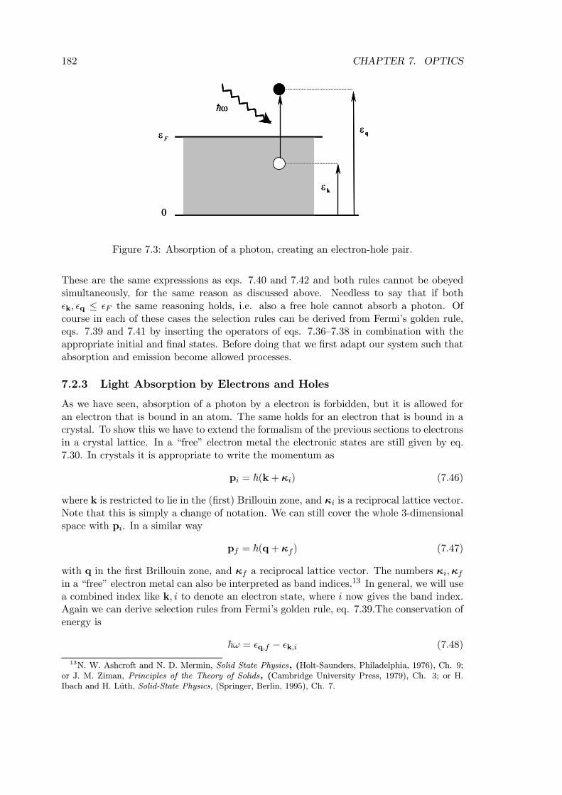
182 CHAPTER 7. OPTICS
Fε
0
εk
εq
ω
Fε
0
εk
εq
ω
Figure 7.3: Absorption of a photon, creating an electron-hole pair.
These are the same expresssions as eqs. 7.40 and 7.42 and both rules cannot be obeyedsimultaneously, for the same reason as discussed above. Needless to say that if both²k, ²q ≤ ²F the same reasoning holds, i.e. also a free hole cannot absorb a photon. Ofcourse in each of these cases the selection rules can be derived from Fermi’s golden rule,eqs. 7.39 and 7.41 by inserting the operators of eqs. 7.36—7.38 in combination with theappropriate initial and final states. Before doing that we first adapt our system such thatabsorption and emission become allowed processes.
7.2.3 Light Absorption by Electrons and Holes
As we have seen, absorption of a photon by a electron is forbidden, but it is allowed foran electron that is bound in an atom. The same holds for an electron that is bound in acrystal. To show this we have to extend the formalism of the previous sections to electronsin a crystal lattice. In a “free” electron metal the electronic states are still given by eq.7.30. In crystals it is appropriate to write the momentum as
pi = ~(k+ κi) (7.46)
where k is restricted to lie in the (first) Brillouin zone, and κi is a reciprocal lattice vector.Note that this is simply a change of notation. We can still cover the whole 3-dimensionalspace with pi. In a similar way
pf = ~(q+ κf ) (7.47)
with q in the first Brillouin zone, and κf a reciprocal lattice vector. The numbers κi,κfin a “free” electron metal can also be interpreted as band indices.13 In general, we will usea combined index like k, i to denote an electron state, where i now gives the band index.Again we can derive selection rules from Fermi’s golden rule, eq. 7.39.The conservation ofenergy is
~ω = ²q,f − ²k,i (7.48)
13N. W. Ashcroft and N. D. Mermin, Solid State Physics, (Holt-Saunders, Philadelphia, 1976), Ch. 9;or J. M. Ziman, Principles of the Theory of Solids, (Cambridge University Press, 1979), Ch. 3; or H.Ibach and H. Luth, Solid-State Physics, (Springer, Berlin, 1995), Ch. 7.
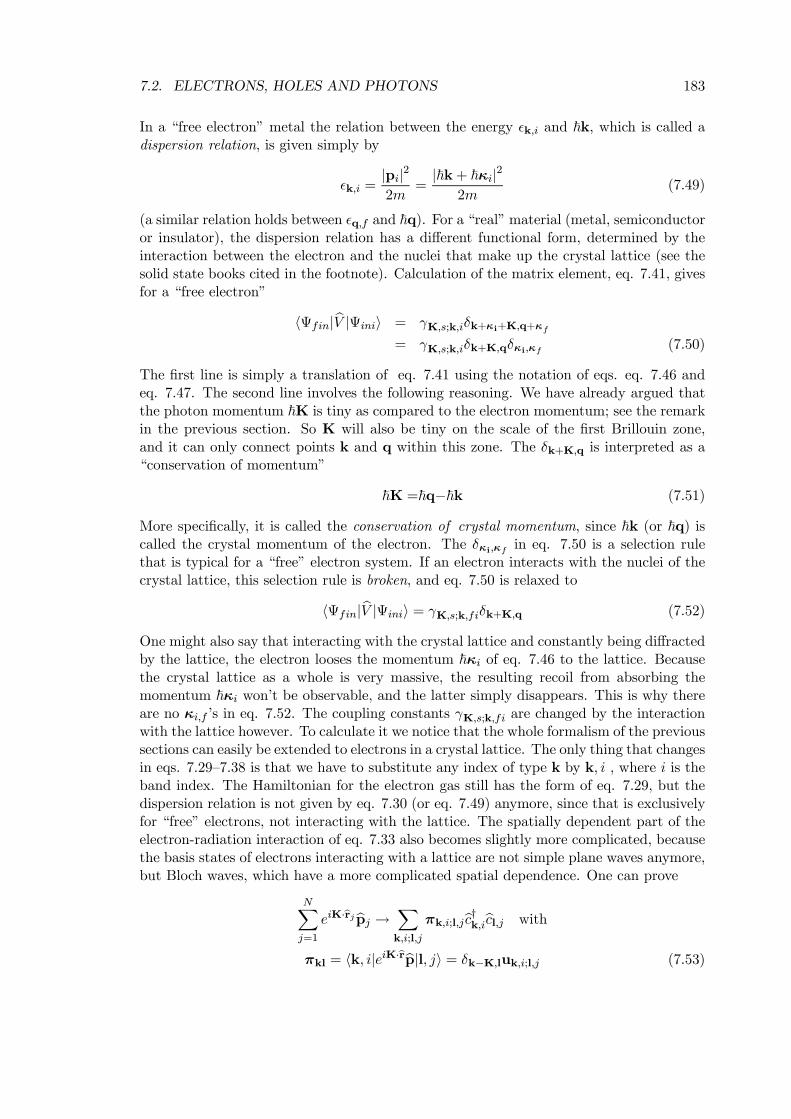
7.2. ELECTRONS, HOLES AND PHOTONS 183
In a “free electron” metal the relation between the energy ²k,i and ~k, which is called adispersion relation, is given simply by
²k,i =|pi|22m
=|~k+ ~κi|2
2m(7.49)
(a similar relation holds between ²q,f and ~q). For a “real” material (metal, semiconductoror insulator), the dispersion relation has a different functional form, determined by theinteraction between the electron and the nuclei that make up the crystal lattice (see thesolid state books cited in the footnote). Calculation of the matrix element, eq. 7.41, givesfor a “free electron”
hΨfin|bV |Ψinii = γK,s;k,iδk+κi+K,q+κf= γK,s;k,iδk+K,qδκi,κf (7.50)
The first line is simply a translation of eq. 7.41 using the notation of eqs. eq. 7.46 andeq. 7.47. The second line involves the following reasoning. We have already argued thatthe photon momentum ~K is tiny as compared to the electron momentum; see the remarkin the previous section. So K will also be tiny on the scale of the first Brillouin zone,and it can only connect points k and q within this zone. The δk+K,q is interpreted as a“conservation of momentum”
~K =~q−~k (7.51)
More specifically, it is called the conservation of crystal momentum, since ~k (or ~q) iscalled the crystal momentum of the electron. The δκi,κf in eq. 7.50 is a selection rulethat is typical for a “free” electron system. If an electron interacts with the nuclei of thecrystal lattice, this selection rule is broken, and eq. 7.50 is relaxed to
hΨfin|bV |Ψinii = γK,s;k,fiδk+K,q (7.52)
One might also say that interacting with the crystal lattice and constantly being diffractedby the lattice, the electron looses the momentum ~κi of eq. 7.46 to the lattice. Becausethe crystal lattice as a whole is very massive, the resulting recoil from absorbing themomentum ~κi won’t be observable, and the latter simply disappears. This is why thereare no κi,f ’s in eq. 7.52. The coupling constants γK,s;k,fi are changed by the interactionwith the lattice however. To calculate it we notice that the whole formalism of the previoussections can easily be extended to electrons in a crystal lattice. The only thing that changesin eqs. 7.29—7.38 is that we have to substitute any index of type k by k, i , where i is theband index. The Hamiltonian for the electron gas still has the form of eq. 7.29, but thedispersion relation is not given by eq. 7.30 (or eq. 7.49) anymore, since that is exclusivelyfor “free” electrons, not interacting with the lattice. The spatially dependent part of theelectron-radiation interaction of eq. 7.33 also becomes slightly more complicated, becausethe basis states of electrons interacting with a lattice are not simple plane waves anymore,but Bloch waves, which have a more complicated spatial dependence. One can prove
NXj=1
eiK·brjbpj → Xk,i;l,j
πk,i;l,jbc†k,ibcl,j with
πkl = hk, i|eiK·brbp|l, ji = δk−K,luk,i;l,j (7.53)
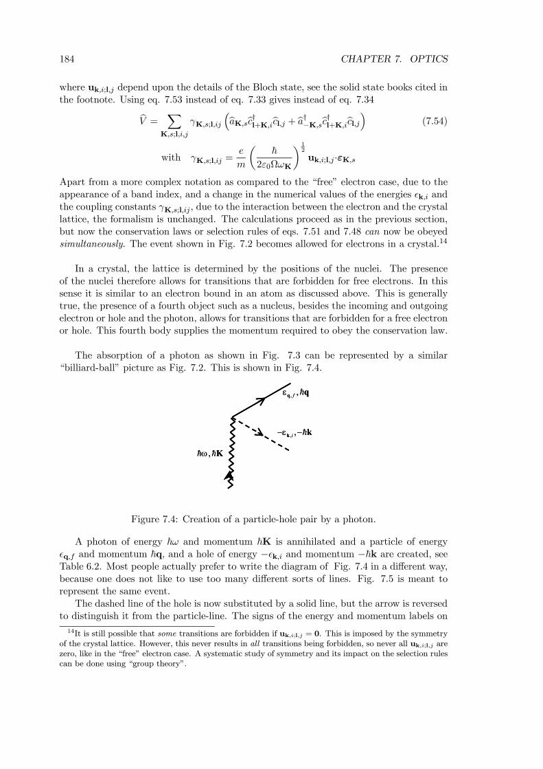
184 CHAPTER 7. OPTICS
where uk,i;l,j depend upon the details of the Bloch state, see the solid state books cited inthe footnote. Using eq. 7.53 instead of eq. 7.33 gives instead of eq. 7.34
bV = XK,s;l,i,j
γK,s;l,ij
³baK,sbc†l+K,ibcl,j + ba†−K,sbc†l+K,ibcl,j´ (7.54)
with γK,s;l,ij =e
m
µ~
2ε0ΩωK
¶ 12
uk,i;l,j ·εK,s
Apart from a more complex notation as compared to the “free” electron case, due to theappearance of a band index, and a change in the numerical values of the energies ²k,i andthe coupling constants γK,s;l,ij , due to the interaction between the electron and the crystallattice, the formalism is unchanged. The calculations proceed as in the previous section,but now the conservation laws or selection rules of eqs. 7.51 and 7.48 can now be obeyedsimultaneously. The event shown in Fig. 7.2 becomes allowed for electrons in a crystal.14
In a crystal, the lattice is determined by the positions of the nuclei. The presenceof the nuclei therefore allows for transitions that are forbidden for free electrons. In thissense it is similar to an electron bound in an atom as discussed above. This is generallytrue, the presence of a fourth object such as a nucleus, besides the incoming and outgoingelectron or hole and the photon, allows for transitions that are forbidden for a free electronor hole. This fourth body supplies the momentum required to obey the conservation law.
The absorption of a photon as shown in Fig. 7.3 can be represented by a similar“billiard-ball” picture as Fig. 7.2. This is shown in Fig. 7.4.
, ,fεq q
,ω K
, ,iε− −k k
, ,fεq q
,ω K
, ,iε− −k k
Figure 7.4: Creation of a particle-hole pair by a photon.
A photon of energy ~ω and momentum ~K is annihilated and a particle of energy²q,f and momentum ~q, and a hole of energy −²k,i and momentum −~k are created, seeTable 6.2. Most people actually prefer to write the diagram of Fig. 7.4 in a different way,because one does not like to use too many different sorts of lines. Fig. 7.5 is meant torepresent the same event.
The dashed line of the hole is now substituted by a solid line, but the arrow is reversedto distinguish it from the particle-line. The signs of the energy and momentum labels on
14It is still possible that some transitions are forbidden if uk,i;l,j = 0. This is imposed by the symmetryof the crystal lattice. However, this never results in all transitions being forbidden, so never all uk,i;l,j arezero, like in the “free” electron case. A systematic study of symmetry and its impact on the selection rulescan be done using “group theory”.
7.2. ELECTRONS, HOLES AND PHOTONS 185
, ,fεq q
,ω K
, ,iεk k
, ,fεq q
,ω K
, ,iεk k
Figure 7.5: Creation of a particle-hole pair by a photon.
the hole-line are also changed to ²k,i and a momentum ~k. The idea is that the “−” signis now supplied by the direction of the arrow, such that the energy and momentum of thehole stays the same as in Fig. 7.4. The time in this diagram increases from left to right,as always. Note therefore that time runs against the arrow in the hole-line (bottom solidline in Fig. 7.5), whereas it runs with the arrow in the particle-line (top solid line in Fig.7.5). There are several reasons for choosing this representation. For instance, by lookingat the diagram one can immediately identify the conservation of energy and momentum,eqs. eq. 7.51 and eq. 7.48, interpreting the diagram as a “circuit”. At the vertex the“sum of all incoming arrows” must be equal to the “sum of all outgoing arrows”. Thisleads to ~ω+ ²k,i = ²q,f and ~K+ ~k =~q, which are the conservation laws. (One alwaysimplicitly assumes that the crystal momentum ~κ is taken care of by the crystal). Theoperator corresponding to this diagram is given by
bU (1)(t, t0) ≡ 1
i~
Z t
t0
dτ bU0(t, τ) hγK,s;k,fi ³baK,s + ba†−K,s´iba†q,fbb†k,i bU0(τ , t0) (7.55)
Note that the middle part now corresponds to the interaction term of eq. 7.36, for which²k ≤ ²F and ²k+K = ²q > ²F , which corresponds to creation of a a particle-hole pair. Tocomplete the calculation we have to sandwich this operator between suitable initial andfinal states. A bit of reflection shows that a suitable inital state is |Ψinii = |0; 0; 1Ki,i.e. zero electrons; zero holes; and one photon in state K. A suitable final state thenis |Ψfini = |1q,f ; 1k,i; 0i, i.e. one electron in state q,f , one hole in state k, i, and zerophotons. The matrix element gives
h1q,f ; 1k,i; 0|hγK,s;k,fi
³baK,s + ba†−K,s´iba†q,fbb†k,i|0; 0; 1Ki = γK,s;k,fiδk+K,q (7.56)
analogous to eq. 7.52. Diagrams like that of Fig. 7.5 are often written without time-labels.You can easily attach them yourself when required. So t0 goes to the bottom of the photonline, τ to the vertex, and the ends of the partcicle and hole lines both get the time label t.
Using such diagrams and playing around with the lines and the arrows allows somequick insight in possible events. For instance, if one flips the solid lines of Fig. 7.5 arounda horizontal axis through the vertex and then rotates them by 90o around the vertex, oneobtains Fig. 7.2. The main difference between Figs. 7.2 and 7.5 is whether the initial stateis above or below the Fermi level, see also Figs. 7.1 and 7.3. The physical interpretation of
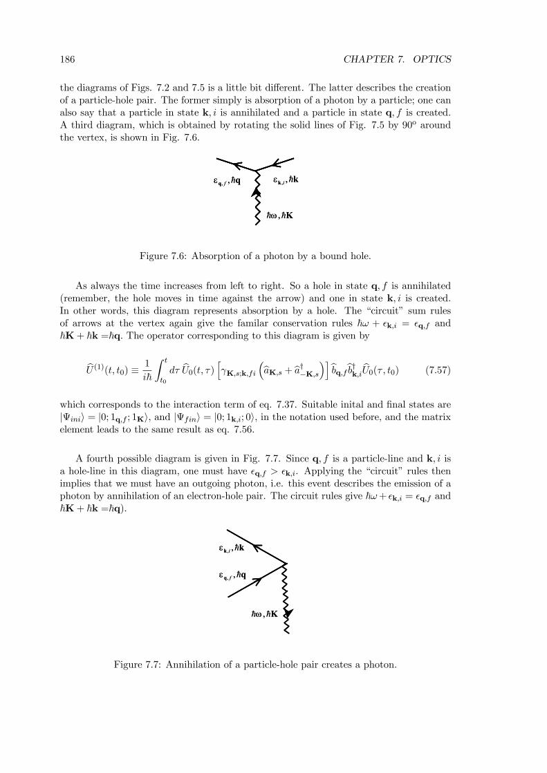
186 CHAPTER 7. OPTICS
the diagrams of Figs. 7.2 and 7.5 is a little bit different. The latter describes the creationof a particle-hole pair. The former simply is absorption of a photon by a particle; one canalso say that a particle in state k, i is annihilated and a particle in state q, f is created.A third diagram, which is obtained by rotating the solid lines of Fig. 7.5 by 90o aroundthe vertex, is shown in Fig. 7.6.
,ω K
, ,iεk k, ,fεq q
,ω K
, ,iεk k, ,fεq q
Figure 7.6: Absorption of a photon by a bound hole.
As always the time increases from left to right. So a hole in state q, f is annihilated(remember, the hole moves in time against the arrow) and one in state k, i is created.In other words, this diagram represents absorption by a hole. The “circuit” sum rulesof arrows at the vertex again give the familar conservation rules ~ω + ²k,i = ²q,f and~K+ ~k =~q. The operator corresponding to this diagram is given by
bU (1)(t, t0) ≡ 1
i~
Z t
t0
dτ bU0(t, τ) hγK,s;k,fi ³baK,s + ba†−K,s´ibbq,fbb†k,i bU0(τ , t0) (7.57)
which corresponds to the interaction term of eq. 7.37. Suitable inital and final states are|Ψinii = |0; 1q,f ; 1Ki, and |Ψfini = |0; 1k,i; 0i, in the notation used before, and the matrixelement leads to the same result as eq. 7.56.
A fourth possible diagram is given in Fig. 7.7. Since q, f is a particle-line and k, i isa hole-line in this diagram, one must have ²q,f > ²k,i. Applying the “circuit” rules thenimplies that we must have an outgoing photon, i.e. this event describes the emission of aphoton by annihilation of an electron-hole pair. The circuit rules give ~ω+ ²k,i = ²q,f and~K+ ~k =~q).
, ,fεq q
,ω K
, ,iεk k
, ,fεq q
,ω K
, ,iεk k
Figure 7.7: Annihilation of a particle-hole pair creates a photon.
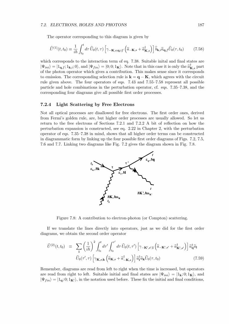
7.2. ELECTRONS, HOLES AND PHOTONS 187
The operator corresponding to this diagram is given by
bU (1)(t, t0) ≡ 1
i~
Z t
t0
dτ bU0(t, τ) hγ−K,s;q,if ³ba−K,s + ba†K,s´ibbk,ibaq,f bU0(τ , t0) (7.58)
which corresponds to the interaction term of eq. 7.38. Suitable inital and final states are|Ψinii = |1q,f ; 1k,i; 0i, and |Ψfini = |0; 0; 1Ki. Note that in this case it is only the ba†K,s partof the photon operator which gives a contribution. This makes sense since it correspondsto emission. The corresponding selection rule is k = q−K, which agrees with the circuitrule given above. The four operators of eqs. 7.43 and 7.55—7.58 represent all possibleparticle and hole combinations in the perturbation operator, cf. eqs. 7.35—7.38, and thecorresponding four diagrams give all possible first order processes.
7.2.4 Light Scattering by Free Electrons
Not all optical processes are disallowed for free electrons. The first order ones, derivedfrom Fermi’s golden rule, are, but higher order processes are usually allowed. So let usreturn to the free electrons of Sections 7.2.1 and 7.2.2 A bit of reflection on how theperturbation expansion is constructed, see eq. 2.22 in Chapter 2, with the perturbationoperator of eqs. 7.35—7.38 in mind, shows that all higher order terms can be constructedin diagrammatic form by linking up the four possible first order diagrams of Figs. 7.2, 7.5,7.6 and 7.7. Linking two diagrams like Fig. 7.2 gives the diagram shown in Fig. 7.8.
, ωKK'', ωKK
,εk k
,εq q0t
0t
t
t
τ'τ
,ε l l
, ωKK'', ωKK
,εk k
,εq q0t
0t
t
t
τ'τ
,ε l l
Figure 7.8: A contribution to electron-photon (or Compton) scattering.
If we translate the lines directly into operators, just as we did for the first orderdiagrams, we obtain the second order operator
bU (2)(t, t0) ≡ Xl
µ1
i~
¶2 Z t
t0
dτ 0Z τ 0
t0
dτ bU0(t, τ 0) hγ−K0,s0;l
³ba−K0,s0 + ba†K0,s0
´iba†qbalbU0(τ 0, τ) hγK,s;k ³baK,s + ba†−K,s´iba†lbak bU0(τ , t0) (7.59)
Remember, diagrams are read from left to right when the time is increased, but operatorsare read from right to left. Suitable initial and final states are |Ψinii = |1k; 0; 1Ki, and|Ψfini = |1q; 0; 1K0i, in the notation used before. These fix the initial and final conditions,
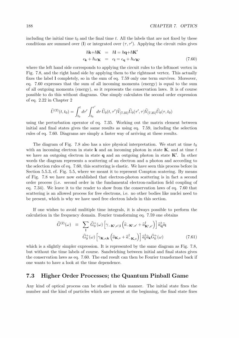
188 CHAPTER 7. OPTICS
including the initial time t0 and the final time t. All the labels that are not fixed by theseconditions are summed over (l) or integrated over (τ , τ 0). Applying the circuit rules gives
~k+~K = ~l = ~q+~K0
²k + ~ωK = ²l = ²q + ~ωK0 (7.60)
where the left hand side corresponds to applying the circuit rules to the leftmost vertex inFig. 7.8, and the right hand side by applying them to the rightmost vertex. This actuallyfixes the label l completely, so in the sum of eq. 7.59 only one term survives. Moreover,eq. 7.60 expresses that the sum of all incoming momenta (energy) is equal to the sumof all outgoing momenta (energy), so it represents the conservation laws. It is of coursepossible to do this without diagrams. One simply calculates the second order expressionof eq. 2.22 in Chapter 2
bU (2)(t, t0) = Z t
t0
dτ 0Z τ 0
t0
dτ bU0(t, τ 0)bV(7.35) bU0(τ 0, τ)bV(7.35) bU0(τ , t0)using the perturbation operator of eq. 7.35. Working out the matrix element betweeninitial and final states gives the same results as using eq. 7.59, including the selectionrules of eq. 7.60. Diagrams are simply a faster way of arriving at these results.
The diagram of Fig. 7.8 also has a nice physical interpretation. We start at time t0with an incoming electron in state k and an incoming photon in state K, and at time twe have an outgoing electron in state q and an outgoing photon in state K0. In otherwords the diagram represents a scattering of an electron and a photon and according tothe selection rules of eq. 7.60, this scattering is elastic. We have seen this process before inSection 5.5.3, cf. Fig. 5.5, where we meant it to represent Compton scatering. By meansof Fig. 7.8 we have now established that electron-photon scattering is in fact a secondorder process (i.e. second order in the fundamental electron-radiation field coupling ofeq. 7.34). We leave it to the reader to show from the conservation laws of eq. 7.60 thatscattering is an allowed process for free electrons, i.e. no other bodies like nuclei need tobe present, which is why we have used free electron labels in this section.
If one wishes to avoid mulitiple time integrals, it is always possible to perform thecalculation in the frequency domain. Fourier transforming eq. 7.59 one obtains
bG(2)(ω) ≡ Xl
bG+0 (ω) hγ−K0,s0;l
³ba−K0,s0 + ba†K0,s0
´iba†qbalbG+0 (ω) hγK,s;k ³baK,s + ba†−K,s´iba†lbak bG+0 (ω) (7.61)
which is a slightly simpler expression. It is represented by the same diagram as Fig. 7.8,but without the time labels of course. Sandwiching between initial and final states givesthe conservation laws as eq. 7.60. The end result can then be Fourier transformed back ifone wants to have a look at the time dependence.
7.3 Higher Order Processes; the Quantum Pinball Game
Any kind of optical process can be studied in this manner. The initial state fixes thenumber and the kind of particles which are present at the beginning, the final state fixes
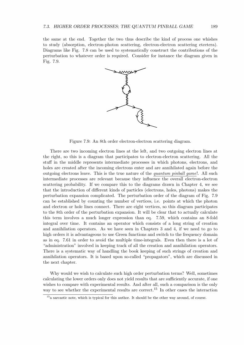
7.3. HIGHER ORDER PROCESSES; THE QUANTUM PINBALL GAME 189
the same at the end. Together the two thus describe the kind of process one whishesto study (absorption, electron-photon scattering, electron-electron scattering etcetera).Diagrams like Fig. 7.8 can be used to systematically construct the contributions of theperturbation to whatever order is required. Consider for instance the diagram given inFig. 7.9.
Figure 7.9: An 8th order electron-electron scattering diagram.
There are two incoming electron lines at the left, and two outgoing electron lines atthe right, so this is a diagram that participates to electron-electron scattering. All thestuff in the middle represents intermediate processes in which photons, electrons, andholes are created after the incoming electrons enter and are annihilated again before theoutgoing electrons leave. This is the true nature of the quantum pinball game!. All suchintermediate processes are relevant because they influence the overall electron-electronscattering probability. If we compare this to the diagrams drawn in Chapter 4, we seethat the introduction of different kinds of particles (electrons, holes, photons) makes theperturbation expansion complicated. The perturbation order of the diagram of Fig. 7.9can be established by counting the number of vertices, i.e. points at which the photonand electron or hole lines connect. There are eight vertices, so this diagram participatesto the 8th order of the perturbation expansion. It will be clear that to actually calculatethis term involves a much longer expression than eq. 7.59, which contains an 8-foldintegral over time. It contains an operator which consists of a long string of creationand annihilation operators. As we have seen in Chapters 3 and 4, if we need to go tohigh orders it is advantageous to use Green functions and switch to the frequency domainas in eq. 7.61 in order to avoid the multiple time-integrals. Even then there is a lot of“administration” involved in keeping track of all the creation and annihilation operators.There is a systematic way of handling the book keeping of such strings of creation andannihilation operators. It is based upon so-called “propagators”, which are discussed inthe next chapter.
Why would we wish to calculate such high order perturbation terms? Well, sometimescalculating the lower orders only does not yield results that are sufficiently accurate, if onewishes to compare with experimental results. And after all, such a comparison is the onlyway to see whether the experimental results are correct.15 In other cases the interaction
15a sarcastic note, which is typical for this author. It should be the other way around, of course.
190 CHAPTER 7. OPTICS
can be so strong that the lower order perturbation terms gives results that are divergent,which clearly is useless. The situation is not hopeless however, because we can use thetechniques presented in Chapters 3 and 4 to sum the complete perturbation series over allorders. However, to be fair, this usually involves approximations. This is the subject ofthe final chapter.
7.4 Appendix I. Interaction of an Electron with an EM field
A watertight derivation of the complete Hamiltonian for electrons and photons would gotoo far here,16 but the following more or less gives the essential idea. Classically, anelectron with charge −e, moving at a velocity r in an electric field E and a magnetic fieldB experiences a Lorentz02 force
F = −eE− e(r×B) (7.62)
and its motion is described by Newton’s law mr = F. It is possible to derive this law ofmotion from the following Lagrangian
L =1
2m|r|2 + eφ− eA · r (7.63)
where φ,A are the usual EM scalar and vector potentials, from which the E and B fieldsare derived as
E = −∇φ− ∂A
∂tand B =∇×A (7.64)
All fields and potentials depend upon (r, t), but sometimes I leave out these arguments toshorten the notation. Look at the Lagrange equations of motion in cartesian coordinates.For the x-degree of freedom one obtains from eq. 7.63
d
dt
µ∂L
∂x
¶− ∂L
∂x=d
dt(mx− eAx)− e
µ∂φ
∂x− ∂Ax
∂xx− ∂Ay
∂xy − ∂Az
∂xz
¶= 0 (7.65)
The first term on the right hand side gives
mx− edAxdt
work out
dAxdt
=∂Ax∂t
+∂Ax∂x
dx
dt+
∂Ax∂y
dy
dt+
∂Ax∂z
dz
dt
Using this in eq. 7.65, and collecting terms gives
mx+ e
µ−∂φ∂x− ∂Ax
∂t
¶+ ey
µ∂Ay∂x− ∂Ax
∂y
¶− ez
µ∂Ax∂z− ∂Az
∂x
¶= mx+ eEx + eyBz − ezBy = mx+ eEx + e(r×B)x = 0 (7.66)
where eq. 7.64 has been used. Obviously this corresponds to Newton’s equation of motionwith a force descibed by eq. 7.62. A similar derivation holds for the y- and z-degrees of
16See R. Loudon, The Quantum Theory of Light, (Clarendon, Oxford, 1981) Ch.8; or the books byCohen-Tannoudji cited before.
7.4. APPENDIX I. INTERACTION OF AN ELECTRON WITH AN EM FIELD 191
freedom, which proves that eq. 7.63 is indeed the correct Lagrangian for an electron in anEM field. If we want to switch to quantum mechanics, we first have to obtain the classicalHamiltonian. The generalized momenta are given by
px =∂L
∂x= mx− eAx (7.67)
Substituting x by y (or z) gives the y (or z) component. The Hamiltonian is then givenby
H = xpx + ypy + zpz − L
=|p+eA|22m
− eφ
=
µ |p|22m− eφ
¶+e
m(A · p) + e2
2m|A|2 (7.68)
expressed in generalized momenta, as it should for a Hamiltonian. Hamilton’s equationslead to the same equations of motion as eq. 7.66, as you can easily check for yourself.The first term in the bottom line of eq. 7.68 describes the motion of the electron in anelectrostatic potential φ(r, t). For instance, in the presence of a nucleus of charge Z in theorigin one has
−eφ(r, t) = −Ze2
|r(t)|just as in eq. 7.1. If another electron is present at position r0 it contributes a Coulombrepulsion term
−eφ(r, t) = e2
|r(t)− r0|and all such electrostatic terms are of course additive. The second and third term inthe bottom line of eq. 7.68 describe the interaction of the electron with the radiationfield, represented by the vector potential A(r, t). Eq. 7.68 can be used to obtain thequantum mechanical Hamiltonian bH, by substituting r(t) → br, p(t) → bp, φ(r, t) → φ(br)and A(r, t)→bA(br) as discussed in the text. Note that, as usual, the time disappears inthe operators. Since we work in the Schrodinger picture, the operators are assumed tobe time-independent, and all time dependence goes into the states (or in the evolutionoperator, which is the same thing).
Starting from eq. 7.68, it is not difficult to produce the Hamiltonian in stone-age formfor an N -electron system
bH =NXi
· bp2i2m
+−Ze2|bri|
¸+1
2
NXi6=j
e2
|bri − brj | (7.69)
+e
m
NXi
³bA(bri)·bpi´+ e2
2m
NXi
bA(bri)·bA(bri) (7.70)
Comparing to the main text, one can see that eq. 7.69 corresponds to the atomic Hamil-tonian bHatom of eq. 7.1. Eq. 7.70 corresponds to the interaction operator bV . One
192 CHAPTER 7. OPTICS
might worry about the order of the operators bA(brj) and bpj . In the classical expressionof eq. 7.68 they can be interchanged freely, but in quantum mechanics brj and bpj arenon-commutating operators. However in this case the order does not matter, if we use theCoulomb gauge, i.e. ∇ ·A =0, see Section 5.5.1. Thus operating on a wave function onegets
bp · bA(br)ψ(r) =~i∇ ·A(r)ψ(r) =~
i[∇ ·A(r)]ψ(r)+~
iA(r)· [∇ψ(r)]
=~iA(r)· [∇ψ(r)]=bA(br) · bpψ(r) (7.71)
i.e. the two operators commutate in the Coulomb gauge and we can safely write for theinteraction operator17
bV = e
m
NXi
bpi·bA(bri) + e2
2m
NXi
bA(bri)·bA(bri) (7.72)
The second sum in this expression actually does not give a contribution to the processesdiscussed in this chapter. So we have skipped this term altogether to arrive at the ex-pression of eq. 7.31. (It is a real term however, and in general one has to take it intoaccount).
7.4.1 Dipole Approximation
For an electron in an atom we did not use eq. 7.72 for the interaction operator, but amuch simpler one, namely
bV = e NXj=1
brj ·bE (7.73)
see eq. 7.6. Let us see how we can derive this. Return to the classical expression of eq.7.68. From classical electrodynamics we know that it is possible to define a so-called gaugefunction χ(r, t) and use it to define new vector and scalar potentials by
A0(r, t) = A(r, t) +∇χ(r, t)φ0(r, t) = φ(r, t)− ∂
∂tχ(r, t) (7.74)
The magnetic and electric fields are not changed by this
B(r, t) = ∇×A0(r, t) =∇×A(r, t)E(r, t) = − ∂
∂tA0(r, t)−∇φ0(r, t) = − ∂
∂tA(r, t)−∇φ(r, t) (7.75)
since ∇×∇χ(r, t) = 0. The transformation of eq. 7.74 is called a gauge transformation.Since the E and B fields are unchanged by a gauge transformation, we can also use thepotentials φ0 and A0 in our classical Hamiltonian of eq. 7.68 instead of φ and A, since itgives the same equations of motion, cf. eq. 7.66.
17If you are not using the Coulomb gauge, you should use the symmetric form 12
³bpi·bA(bri)+bA(bri)·bpi´.
7.5. APPENDIX II. RELATIVISTIC ELECTRONS AND HOLES 193
The key element for the atom is the so-called long wave length approximation, wherewe assume that the wave length of the EM radiation is much larger than the size of theatom. In this limit we can treat the radiation field as being homogeneous, i.e. spatiallyindependent, so A(r, t) ≈ A(t). We now apply two consecutive gauge transformations.The first one is defined by
χ(r, t) =e
m
Z t
|A(r, t0)|2dt0 (7.76)
which gives
A0(r, t) = A(r, t) +e
m
Z t
∇|A(r, t0)|2dt0 ≈ A(t)
φ0(r, t) = φ(r, t)− e
m|A(r, t)|2 (7.77)
where the first line holds because of the long wave length approximation. Using thetransformed potentials φ0 and A0 in eq. 7.68 instead of φ and A gives
H =
µ |p|22m− eφ
¶+e
m(A · p) (7.78)
i.e. we got rid off the |A|2 term. Now apply a second gauge transformation defined as
χ(r, t) = −r ·A(t) (7.79)
and get
A0(r, t) = A(t) +∇χ(r, t) = 0φ0(r, t) = φ(r, t)− ∂
∂tχ(r, t) = φ(r, t)− r ·E(t) (7.80)
Again, using the transformed potentials φ0 and A0 in eq. 7.80 instead of φ and A gives
H =
µ |p|22m− eφ
¶+ er ·E(t) (7.81)
Transforming this into a quantum mechanical operator, we observe that the last term inthis expression gives the interaction operator bV of eq. 7.73. Note these gauge transfor-mation tricks only work in the long wave length limit, i.e. when the spatial dependence ofthe fields can be neglected. This is valid for small systems like atoms, but in other casesthe more general form of eq. 7.72 has to be used.
7.5 Appendix II. Relativistic Electrons and Holes
I have carefully discussed the direction of the particle and hole lines in Section 7.2, but Ihave not talked much about the photon lines, which I have drawn almost vertically. Thereason is that we have been doing non-relativistic quantum mechanics (the Schrodingerequation is non-relativistic). The speed of light is always much larger than the speed ofthe electrons and holes. Photons move very fast, so letting time increase from left to right,
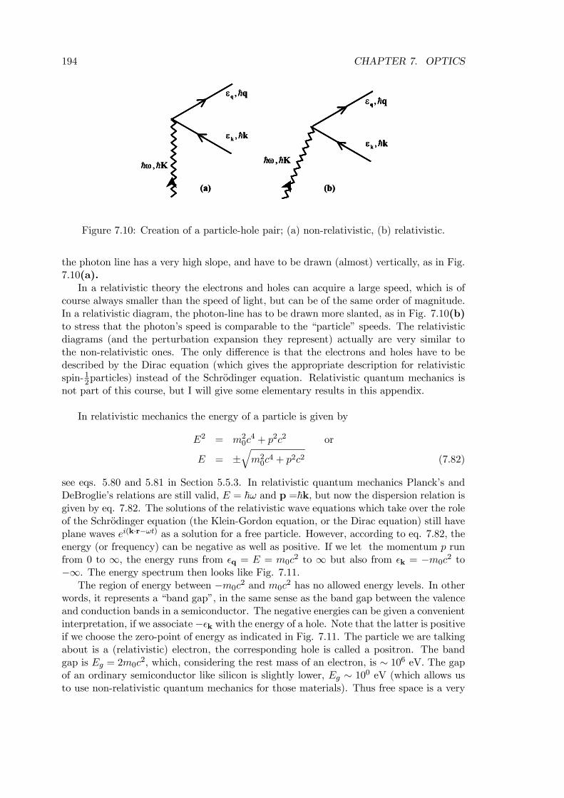
194 CHAPTER 7. OPTICS
,εq q
,ω K
,εk k
(a)
,εq q
,ω K
,εk k
(b)
,εq q
,ω K
,εk k
(a)
,εq q
,ω K
,εk k
(a)
,εq q
,ω K
,εk k
(b)
,εq q
,ω K
,εk k
,εq q
,ω K
,εk k
(b)
Figure 7.10: Creation of a particle-hole pair; (a) non-relativistic, (b) relativistic.
the photon line has a very high slope, and have to be drawn (almost) vertically, as in Fig.7.10(a).
In a relativistic theory the electrons and holes can acquire a large speed, which is ofcourse always smaller than the speed of light, but can be of the same order of magnitude.In a relativistic diagram, the photon-line has to be drawn more slanted, as in Fig. 7.10(b)to stress that the photon’s speed is comparable to the “particle” speeds. The relativisticdiagrams (and the perturbation expansion they represent) actually are very similar tothe non-relativistic ones. The only difference is that the electrons and holes have to bedescribed by the Dirac equation (which gives the appropriate description for relativisticspin-12particles) instead of the Schrodinger equation. Relativistic quantum mechanics isnot part of this course, but I will give some elementary results in this appendix.
In relativistic mechanics the energy of a particle is given by
E2 = m20c4 + p2c2 or
E = ±qm20c
4 + p2c2 (7.82)
see eqs. 5.80 and 5.81 in Section 5.5.3. In relativistic quantum mechanics Planck’s andDeBroglie’s relations are still valid, E = ~ω and p =~k, but now the dispersion relation isgiven by eq. 7.82. The solutions of the relativistic wave equations which take over the roleof the Schrodinger equation (the Klein-Gordon equation, or the Dirac equation) still haveplane waves ei(k·r−ωt) as a solution for a free particle. However, according to eq. 7.82, theenergy (or frequency) can be negative as well as positive. If we let the momentum p runfrom 0 to ∞, the energy runs from ²q = E = m0c
2 to ∞ but also from ²k = −m0c2 to
−∞. The energy spectrum then looks like Fig. 7.11.The region of energy between −m0c2 and m0c
2 has no allowed energy levels. In otherwords, it represents a “band gap”, in the same sense as the band gap between the valenceand conduction bands in a semiconductor. The negative energies can be given a convenientinterpretation, if we associate−²k with the energy of a hole. Note that the latter is positiveif we choose the zero-point of energy as indicated in Fig. 7.11. The particle we are talkingabout is a (relativistic) electron, the corresponding hole is called a positron. The bandgap is Eg = 2m0c
2, which, considering the rest mass of an electron, is ∼ 106 eV. The gapof an ordinary semiconductor like silicon is slightly lower, Eg ∼ 100 eV (which allows usto use non-relativistic quantum mechanics for those materials). Thus free space is a very
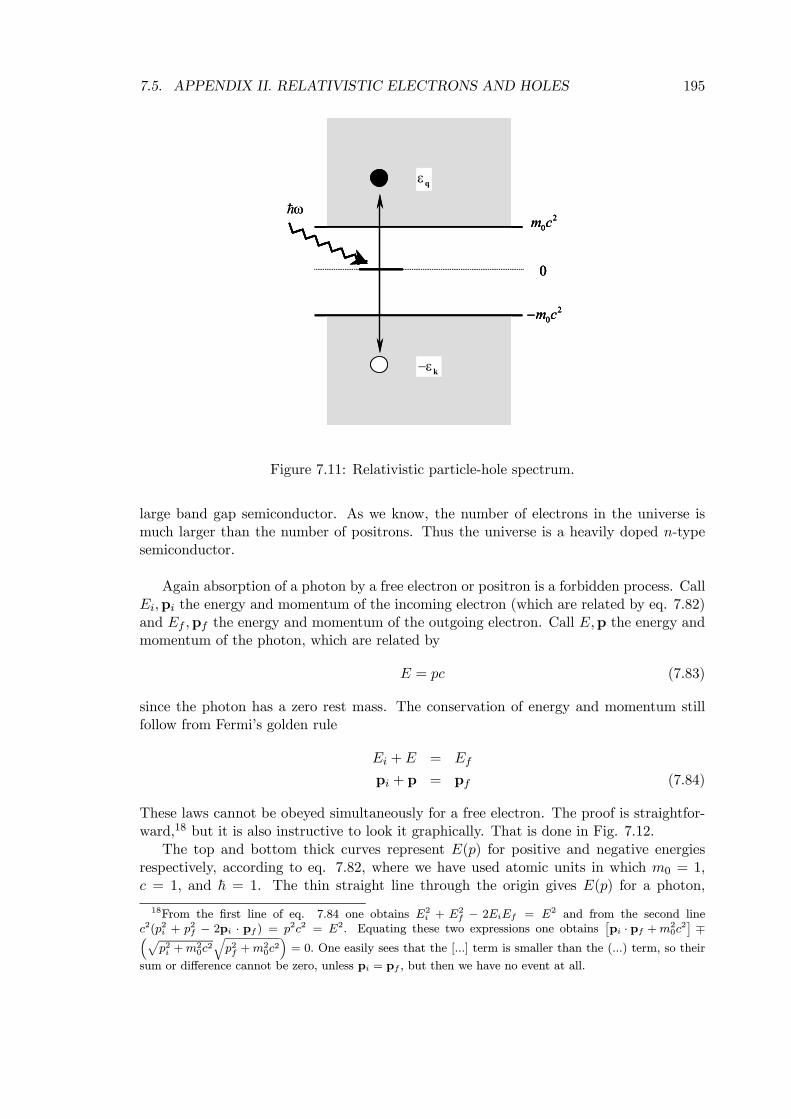
7.5. APPENDIX II. RELATIVISTIC ELECTRONS AND HOLES 195
ε− k
20m c
0
20m c−
εq
ω
ε− k
20m c
0
20m c−
20m c
0
20m c−
εq
ω
Figure 7.11: Relativistic particle-hole spectrum.
large band gap semiconductor. As we know, the number of electrons in the universe ismuch larger than the number of positrons. Thus the universe is a heavily doped n-typesemiconductor.
Again absorption of a photon by a free electron or positron is a forbidden process. CallEi,pi the energy and momentum of the incoming electron (which are related by eq. 7.82)and Ef ,pf the energy and momentum of the outgoing electron. Call E,p the energy andmomentum of the photon, which are related by
E = pc (7.83)
since the photon has a zero rest mass. The conservation of energy and momentum stillfollow from Fermi’s golden rule
Ei +E = Ef
pi + p = pf (7.84)
These laws cannot be obeyed simultaneously for a free electron. The proof is straightfor-ward,18 but it is also instructive to look it graphically. That is done in Fig. 7.12.
The top and bottom thick curves represent E(p) for positive and negative energiesrespectively, according to eq. 7.82, where we have used atomic units in which m0 = 1,c = 1, and ~ = 1. The thin straight line through the origin gives E(p) for a photon,
18From the first line of eq. 7.84 one obtains E2i + E2f − 2EiEf = E2 and from the second linec2(p2i + p
2f − 2pi · pf ) = p2c2 = E2. Equating these two expressions one obtains
£pi · pf +m2
0c2¤ ∓³p
p2i +m20c2qp2f +m
20c2´= 0. One easily sees that the [...] term is smaller than the (...) term, so their
sum or difference cannot be zero, unless pi = pf , but then we have no event at all.
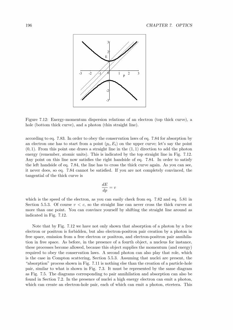
196 CHAPTER 7. OPTICS
-3
-2
-1
0
1
2
3
E
-3 -2 -1 1 2 3p
Figure 7.12: Energy-momentum dispersion relations of an electron (top thick curve), ahole (bottom thick curve), and a photon (thin straight line).
according to eq. 7.83. In order to obey the conservation laws of eq. 7.84 for absorption byan electron one has to start from a point (pi, Ei) on the upper curve; let’s say the point(0, 1). From this point one draws a straight line in the (1, 1) direction to add the photonenergy (remember, atomic units). This is indicated by the top straight line in Fig. 7.12.Any point on this line now satisfies the right handside of eq. 7.84. In order to satisfythe left handside of eq. 7.84, the line has to cross the thick curve again. As you can see,it never does, so eq. 7.84 cannot be satisfied. If you are not completely convinced, thetangential of the thick curve is
dE
dp= v
which is the speed of the electron, as you can easily check from eq. 7.82 and eq. 5.81 inSection 5.5.3. Of course v < c, so the straight line can never cross the thick curves atmore than one point. You can convince yourself by shifting the straight line around asindicated in Fig. 7.12.
Note that by Fig. 7.12 we have not only shown that absorption of a photon by a freeelectron or positron is forbidden, but also electron-positron pair creation by a photon infree space, emission from a free electron or positron, and electron-positron pair annihila-tion in free space. As before, in the presence of a fourth object, a nucleus for instance,these processes become allowed, because this object supplies the momentum (and energy)required to obey the conservation laws. A second photon can also play that role, whichis the case in Compton scattering, Section 5.5.3. Assuming that nuclei are present, the“absorption” process shown in Fig. 7.11 is nothing else than the creation of a particle-holepair, similar to what is shown in Fig. 7.3. It must be represented by the same diagramas Fig. 7.5. The diagrams corresponding to pair annihilation and absorption can also befound in Section 7.2. In the presence of nuclei a high energy electron can emit a photon,which can create an electron-hole pair, each of which can emit a photon, etcetera. This
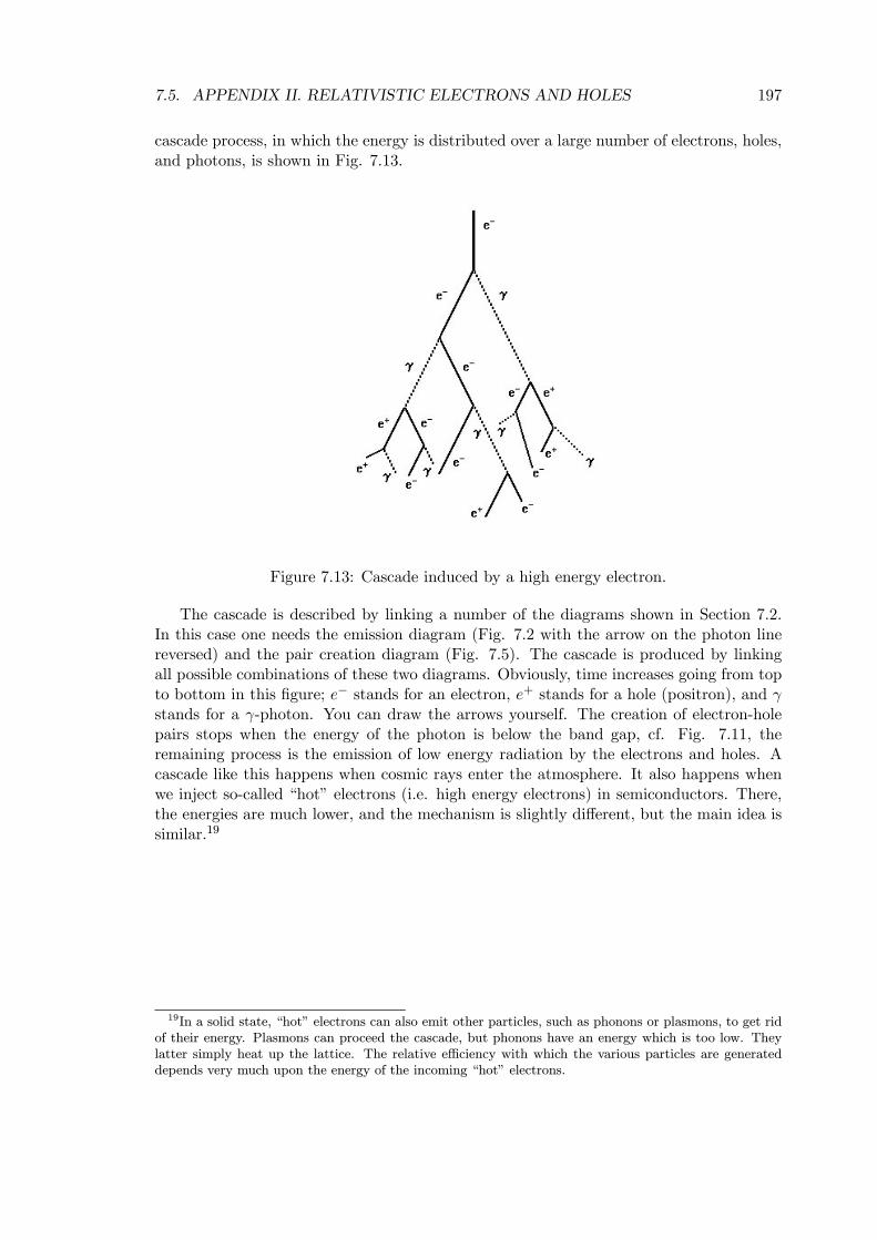
7.5. APPENDIX II. RELATIVISTIC ELECTRONS AND HOLES 197
cascade process, in which the energy is distributed over a large number of electrons, holes,and photons, is shown in Fig. 7.13.
Figure 7.13: Cascade induced by a high energy electron.
The cascade is described by linking a number of the diagrams shown in Section 7.2.In this case one needs the emission diagram (Fig. 7.2 with the arrow on the photon linereversed) and the pair creation diagram (Fig. 7.5). The cascade is produced by linkingall possible combinations of these two diagrams. Obviously, time increases going from topto bottom in this figure; e− stands for an electron, e+ stands for a hole (positron), and γstands for a γ-photon. You can draw the arrows yourself. The creation of electron-holepairs stops when the energy of the photon is below the band gap, cf. Fig. 7.11, theremaining process is the emission of low energy radiation by the electrons and holes. Acascade like this happens when cosmic rays enter the atmosphere. It also happens whenwe inject so-called “hot” electrons (i.e. high energy electrons) in semiconductors. There,the energies are much lower, and the mechanism is slightly different, but the main idea issimilar.19
19In a solid state, “hot” electrons can also emit other particles, such as phonons or plasmons, to get ridof their energy. Plasmons can proceed the cascade, but phonons have an energy which is too low. Theylatter simply heat up the lattice. The relative efficiency with which the various particles are generateddepends very much upon the energy of the incoming “hot” electrons.

198 CHAPTER 7. OPTICS
Part III
Interacting Particles
199

Chapter 8
Propagators and Diagrams
“...You might say, “My Quetzalcoatl! What tedium—counting beans, putting them in, taking them
out—what a job!” To which the priest would reply, “That’s why we have the rules for the bars and
the dots. The rules are tricky, but they are a much more efficient way of getting the answer than
by counting beans...””, Richard Feynman, QED.
Chapters 2, 3, 4 and 7 all dealed with the following question. Suppose at a time t = t0we prepare our system in a state |ii, what is the probability that at a later time t = t1the system will be in a state |fi? The answer to that question is given by the transitionprobability
Wi→f =¯Df¯ bU (t1, t0)¯ iE¯2 (8.1)
where bU(t1, t0) is the time evolution operator. We handled this expression using pertur-bation theory. In first order (the Born approximation) this gave us Fermi’s golden rule.Expansion and summation of the whole perturbation series was possible using Fouriertransforms and Green functions. We have encountered several examples for which we cal-culated these transition probabilities. Unfortunately, but not surprisingly, there are manyphysical systems which are too complicated for such “exact” calculations. In particularthis is true for systems comprising many interacting particles.1 We have to change ourtune and, instead of trying to find exact solutions, we must strive to find reasonable ap-proximations that cover the essential physics of the system. For a many particle systemthe tools of the second quantization formalism are especially handy in achieving this goal.
In the first section we will define a very important quantity called the single particlepropagator (also called the single particle Green function; it is related to the Green func-tions we encountered before). It plays a vital role in interpreting prototype “typical”experiments. In this chapter this propagator will be applied to cases of increasing com-plexity. In comparison with the previous chapter, we go back to systems that involve onekind of particle (or two kinds if you want, a particle and its anti-particle; the two alwaysgo together). We kick off with just a single particle, where we will recover the results ofChapter 4. Then we will treat an example of a system which consists of many particleswith a very simple interaction. This rounds up the cases that are, in principle, exactly
1In fact, there is not a single, non-trivial (i.e. in which the particles interact with each other), many-body system that can be solved exactly, neither in quantum, nor in classical mechanics. The situation ishopeless but not desperate, since in many cases we can find reasonable approximations.
201
202 CHAPTER 8. PROPAGATORS AND DIAGRAMS
solvable, although already the latter will be far from trivial as we will see. A short dis-cussion is then given of the very important physical system in which the particles havepairwise interactions. The last section introduces the so-called spectral function, whichplays a vital role both in the interpretation of experiments and of the formal propertiesof the propagator. This is used to give an analysis of two “real” experiments, namelyphotoemission and inverse photoemission. The two appendices give an introduction to themathematical complexities of many interacting particle systems.
8.1 The Single Particle Propagator
”The time has come,” the Walrus said,
”To talk of many things:
Of shoes—and ships—and sealing-wax—
Of cabbages—and kings—
And why the sea is boiling hot—
And whether pigs have wings.”, Lewis Caroll, The Walrus and the Carpenter.
We “prepare” a specific initial state,
|i(t0)i = bc†i bU (t0, 0) |0i (8.2)
i.e. we start our system at t = 0 in a state |0i, which we propagate to t = t0. In most ofour applications |0i will be the ground state of the system (the vacuum state), hence the
notation. At t0 we create a particle in state |ii by letting bc†i operate on |0i. We write thefinal state as
|f(t1)i = bc†f bU (t1, 0) |0i (8.3)
with a similar interpretation. The transition probability is of course still given by eq. 8.1.We can write the matrix element asD
f(t1)¯ bU (t1, t0)¯ i(t0)E = D0 ¯ bU † (t1, 0)bcf bU (t1, t0)bc†i bU (t0, 0)¯ 0E (8.4)
and use
bU (t1, t0) = bU (t1, 0) bU (0, t0) = bU (t1, 0) bU † (t0, 0)By defining the so-called “Heisenberg” operators as in Section 2.6, eq. 2.63 (dropping the“H” and “S” subscripts)
bck(t) = bU † (t, 0)bck bU (t, 0)bc†k(t) = bU † (t, 0)bc†k bU (t, 0) (8.5)
we then arrive atDf(t1)
¯ bU (t1, t0)¯ i(t0)E =D0¯bcf (t1)bc†i (t0)¯ 0E
≡ i~G+(f, i, t1 − t0) ; t1 > t0 (8.6)
8.1. THE SINGLE PARTICLE PROPAGATOR 203
This quantity plays a prominent role in many-particle physics. It is called the single-particle propagator .2 We used the notation G+ because in view of Chapters 3 and 4, weare obviously dealing with a matrix element of a Green function operator, see in particularSections 3.2.1 and 4.2. Such matrix elements are called Green functions (and rightly so,since they form a representation of the Green function operator on a basis set), see themathematical intermezzo in Section 3.2.1 or eq. 4.20 in Section 4.2. A synonym for thephrase single-particle propagator therefore is single-particle Green function.3 In view ofChapter 7 it will be clear that one can also look at more complicated propagators. Forinstance Fig. 7.9 in Section 7.3 descibes an event in which the initial state contains twoparticles and also the final state contains two. Corresponding “two-particle” propagatorsand Green functions exist, but we won’t consider them in this course. Once you knowhow to deal with the “single-particle propagator”, it is straight-forward to extend thisknowledge to other propagators. So whenever I use the word “propagator” in these notes,the “single-particle propagator” is meant.
In Chapter 3 we used a Dyson expansion for the Green function operator to sumthe perturbation series resulting from a perturbing potential bV . In Chapter 4 we did asimilar expansion for a Green function (matrix element) instead of the operator, using aperturbation series in terms of a quantity called the self-energy Σ. The latter techniqueproves to be more versatile and also applicable to many particle systems. Note that eq.8.6 is very straight-forward to interpret if we read it from right to left. We start with thesystem in the vacuum state |0i. At t = t0 we create a particle by bc†i in the state i and ata later time t = t1, we probe by applying bcf the probability amplitude that the particle isin state f .
8.1.1 A Gedanken Experiment
The physical idea behind the propagator is to mimick the “typical” experiment of Fig.3.1. At some initial time t0 we send in a particle into the system, which is in state |ki,having a well-defined energy ²k and momentum ~k. From the point of view of the systemstarting in its ground state |0i, at time t0 suddenly a (extra) particle appears, which iscreated in |ki by bc†k. At some later time we check the probability of detecting this particlein state |li (with a well-defined energy ²l and momentum ~l) and the system in its originalstate |0i. “Detection” necessarily involves annihilation of the particle, which admittedlyis not very subttle. This “gedanken”-experiment is shown in Fig. 8.1.
This theoretical gedanken experiment is the simplest thing you can do in relation tothe “typical” experiment of Fig. 3.1. If you are an experimentalist, you may wonder howthis “creation of a particle” can be done in practice. The final sections of this chapter givesome examples of real experiments: (inverse) photo-emission. Real experiments are gen-erally much more complicated than the gedanken experiment of Fig. 8.1. A whole chainof events is required to create and detect particles. For a start, one needs a source forcreating particles, e.g. an electron gun to produce electrons or a laser to produce photons.Then the particles should penetrate the boundaries (surfaces) of the system, before theycan propagate through the system. The same is true for emerging particles; these again
2Since bU(t1, t0) = exp h− i~ (t1 − t0) bHi and we assume bH to be time-independent, it is time differences
(t1 − t0) that appear everywhere.3Mattuck’s eqs. 3.3 and 4.29 describe the same thing in words. The full mathematical discussion is
found in his chapter 9.
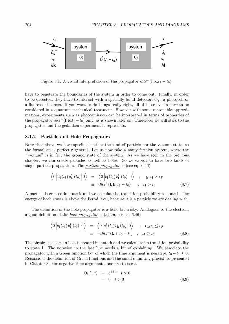
204 CHAPTER 8. PROPAGATORS AND DIAGRAMS
system
⟩0|
system
⟩0|+kakεk
lalεl
t0 t1
)(ˆ01 ttU −
Figure 8.1: A visual interpretation of the propagator i~G+(l,k,t1 − t0).
have to penetrate the boundaries of the system in order to come out. Finally, in orderto be detected, they have to interact with a specially build detector, e.g. a photocell ora fluorescent screen. If you want to do things really right, all of these events have to beconsidered in a quantum mechanical treatment. However with some reasonable approxi-mations, experiments such as photoemission can be interpreted in terms of properties ofthe propagator i~G+(l,k,t1− t0) only, as is shown later on. Therefore, we will stick to thepropagator and the gedanken experiment it represents.
8.1.2 Particle and Hole Propagators
Note that above we have specified neither the kind of particle nor the vacuum state, sothe formalism is perfectly general. Let us now take a many fermion system, where the“vacuum” is in fact the ground state of the system. As we have seen in the previouschapter, we can create particles as well as holes. So we expect to have two kinds ofsingle-particle propagators. The particle propagator is (see eq. 6.46)D
0¯bal (t1)ba†k (t0)¯ 0E =
D0¯bcl (t1)bc†k (t0)¯ 0E ; ²k, ²l > ²F
≡ i~G+(l,k, t1 − t0) ; t1 > t0 (8.7)
A particle is created in state k and we calculate its transition probability to state l. Theenergy of both states is above the Fermi level, because it is a particle we are dealing with.
The definition of the hole propagator is a little bit tricky. Analogous to the electron,a good definition of the hole propagator is (again, see eq. 6.46)D
0¯bbl (t1)bb†k (t0)¯ 0E =
D0¯bc†l (t1)bck (t0)¯ 0E ; ²k, ²l ≤ ²F
≡ −i~G−(k, l, t0 − t1) ; t1 ≥ t0 (8.8)
The physics is clear; an hole is created in state k and we calculate its transition probabilityto state l. The notation in the last line needs a bit of explaining. We associate thepropagator with a Green function G− of which the time argument is negative, t0− t1 ≤ 0.Reconsider the definition of Green functions and the small δ limiting procedure presentedin Chapter 3. For negative time arguments, one has to use a
Θδ (−t) = e+δ.t t ≤ 0= 0 t > 0 (8.9)
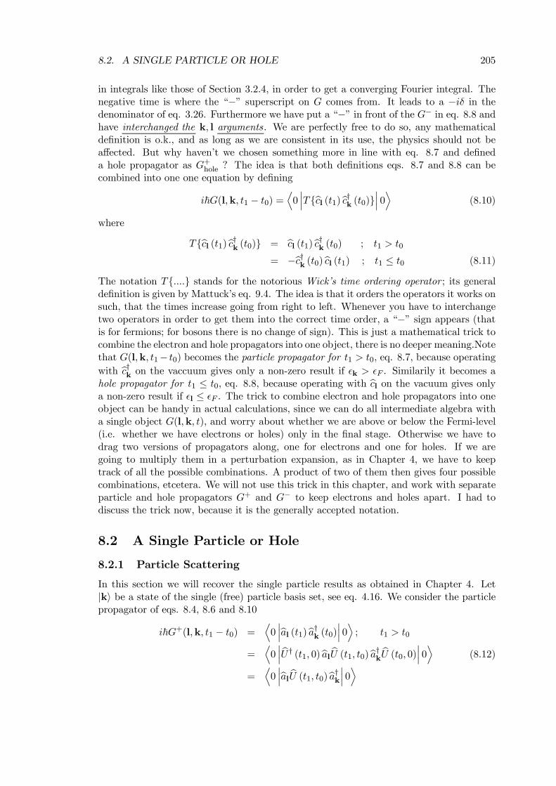
8.2. A SINGLE PARTICLE OR HOLE 205
in integrals like those of Section 3.2.4, in order to get a converging Fourier integral. Thenegative time is where the “−” superscript on G comes from. It leads to a −iδ in thedenominator of eq. 3.26. Furthermore we have put a “−” in front of the G− in eq. 8.8 andhave interchanged the k, l arguments. We are perfectly free to do so, any mathematicaldefinition is o.k., and as long as we are consistent in its use, the physics should not beaffected. But why haven’t we chosen something more in line with eq. 8.7 and defineda hole propagator as G+hole ? The idea is that both definitions eqs. 8.7 and 8.8 can becombined into one one equation by defining
i~G(l,k, t1 − t0) =D0¯Tbcl (t1)bc†k (t0)¯ 0E (8.10)
where
Tbcl (t1)bc†k (t0) = bcl (t1)bc†k (t0) ; t1 > t0
= −bc†k (t0)bcl (t1) ; t1 ≤ t0 (8.11)
The notation T.... stands for the notorious Wick’s time ordering operator ; its generaldefinition is given by Mattuck’s eq. 9.4. The idea is that it orders the operators it works onsuch, that the times increase going from right to left. Whenever you have to interchangetwo operators in order to get them into the correct time order, a “−” sign appears (thatis for fermions; for bosons there is no change of sign). This is just a mathematical trick tocombine the electron and hole propagators into one object, there is no deeper meaning.Notethat G(l,k, t1− t0) becomes the particle propagator for t1 > t0, eq. 8.7, because operatingwith bc†k on the vaccuum gives only a non-zero result if ²k > ²F . Similarily it becomes ahole propagator for t1 ≤ t0, eq. 8.8, because operating with bcl on the vacuum gives onlya non-zero result if ²l ≤ ²F . The trick to combine electron and hole propagators into oneobject can be handy in actual calculations, since we can do all intermediate algebra witha single object G(l,k, t), and worry about whether we are above or below the Fermi-level(i.e. whether we have electrons or holes) only in the final stage. Otherwise we have todrag two versions of propagators along, one for electrons and one for holes. If we aregoing to multiply them in a perturbation expansion, as in Chapter 4, we have to keeptrack of all the possible combinations. A product of two of them then gives four possiblecombinations, etcetera. We will not use this trick in this chapter, and work with separateparticle and hole propagators G+ and G− to keep electrons and holes apart. I had todiscuss the trick now, because it is the generally accepted notation.
8.2 A Single Particle or Hole
8.2.1 Particle Scattering
In this section we will recover the single particle results as obtained in Chapter 4. Let|ki be a state of the single (free) particle basis set, see eq. 4.16. We consider the particlepropagator of eqs. 8.4, 8.6 and 8.10
i~G+(l,k, t1 − t0) =D0¯bal (t1)ba†k (t0)¯ 0E ; t1 > t0
=D0¯ bU † (t1, 0)bal bU (t1, t0)ba†k bU (t0, 0)¯ 0E (8.12)
=D0¯bal bU (t1, t0)ba†k ¯ 0E
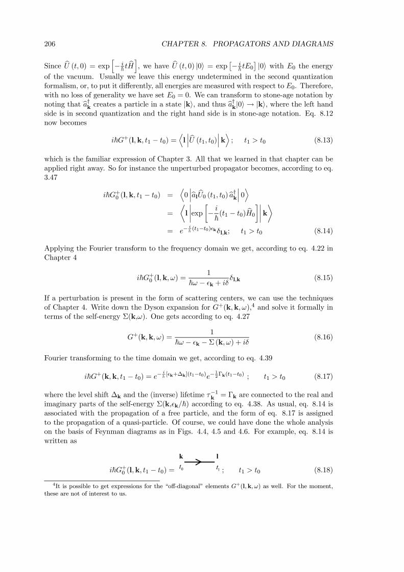
206 CHAPTER 8. PROPAGATORS AND DIAGRAMS
Since bU (t, 0) = exph− i~ tbHi, we have bU (t, 0) |0i = exp
£− i~ tE0
¤ |0i with E0 the energyof the vacuum. Usually we leave this energy undetermined in the second quantizationformalism, or, to put it differently, all energies are measured with respect to E0. Therefore,with no loss of generality we have set E0 = 0. We can transform to stone-age notation bynoting that ba†k creates a particle in a state |ki, and thus ba†k|0i→ |ki, where the left handside is in second quantization and the right hand side is in stone-age notation. Eq. 8.12now becomes
i~G+(l,k, t1 − t0) =Dl¯ bU (t1, t0)¯kE ; t1 > t0 (8.13)
which is the familiar expression of Chapter 3. All that we learned in that chapter can beapplied right away. So for instance the unperturbed propagator becomes, according to eq.3.47
i~G+0 (l,k, t1 − t0) =D0¯bal bU0 (t1, t0)ba†k ¯ 0E
=
¿l
¯exp
·− i~(t1 − t0) bH0¸¯kÀ
= e−i~ (t1−t0)²kδl,k; t1 > t0 (8.14)
Applying the Fourier transform to the frequency domain we get, according to eq. 4.22 inChapter 4
i~G+0 (l,k,ω) =1
~ω − ²k + iδ δl,k (8.15)
If a perturbation is present in the form of scattering centers, we can use the techniquesof Chapter 4. Write down the Dyson expansion for G+(k,k,ω),4 and solve it formally interms of the self-energy Σ(k,ω). One gets according to eq. 4.27
G+(k,k,ω) =1
~ω − ²k − Σ (k,ω) + iδ (8.16)
Fourier transforming to the time domain we get, according to eq. 4.39
i~G+(k,k, t1 − t0) = e− i~ [²k+∆k](t1−t0)e−
12Γk(t1−t0) ; t1 > t0 (8.17)
where the level shift ∆k and the (inverse) lifetime τ−1k = Γk are connected to the real and
imaginary parts of the self-energy Σ(k,²k/~) according to eq. 4.38. As usual, eq. 8.14 isassociated with the propagation of a free particle, and the form of eq. 8.17 is assignedto the propagation of a quasi-particle. Of course, we could have done the whole analysison the basis of Feynman diagrams as in Figs. 4.4, 4.5 and 4.6. For example, eq. 8.14 iswritten as
i~G+0 (l,k, t1 − t0) = 0tk
1tl
; t1 > t0 (8.18)
4It is possible to get expressions for the “off-diagonal” elements G+(l,k,ω) as well. For the moment,these are not of interest to us.
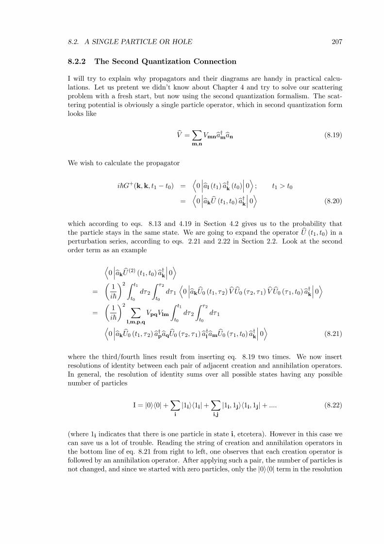
8.2. A SINGLE PARTICLE OR HOLE 207
8.2.2 The Second Quantization Connection
I will try to explain why propagators and their diagrams are handy in practical calcu-lations. Let us pretent we didn’t know about Chapter 4 and try to solve our scatteringproblem with a fresh start, but now using the second quantization formalism. The scat-tering potential is obviously a single particle operator, which in second quantization formlooks like
bV =Xm,n
Vmnba†mban (8.19)
We wish to calculate the propagator
i~G+(k,k, t1 − t0) =D0¯bal (t1)ba†k (t0)¯ 0E ; t1 > t0
=D0¯bak bU (t1, t0)ba†k ¯ 0E (8.20)
which according to eqs. 8.13 and 4.19 in Section 4.2 gives us to the probability thatthe particle stays in the same state. We are going to expand the operator bU (t1, t0) in aperturbation series, according to eqs. 2.21 and 2.22 in Section 2.2. Look at the secondorder term as an example
D0¯bak bU (2) (t1, t0)ba†k ¯ 0E
=
µ1
i~
¶2 Z t1
t0
dτ2
Z τ2
t0
dτ1
D0¯bak bU0 (t1, τ2) bV bU0 (τ2, τ1) bV bU0 (τ1, t0)ba†k ¯ 0E
=
µ1
i~
¶2 Xl,m,p,q
VpqVlm
Z t1
t0
dτ2
Z τ2
t0
dτ1D0¯bak bU0 (t1, τ2)ba†pbaq bU0 (τ2, τ1)ba†lbam bU0 (τ1, t0)ba†k ¯ 0E (8.21)
where the third/fourth lines result from inserting eq. 8.19 two times. We now insertresolutions of identity between each pair of adjacent creation and annihilation operators.In general, the resolution of identity sums over all possible states having any possiblenumber of particles
I = |0ih0|+Xi
|1iih1i|+Xi,j
|1i, 1jih1i, 1j|+ .... (8.22)
(where 1i indicates that there is one particle in state i, etcetera). However in this case wecan save us a lot of trouble. Reading the string of creation and annihilation operators inthe bottom line of eq. 8.21 from right to left, one observes that each creation operator isfollowed by an annihilation operator. After applying such a pair, the number of particles isnot changed, and since we started with zero particles, only the |0ih0| term in the resolution
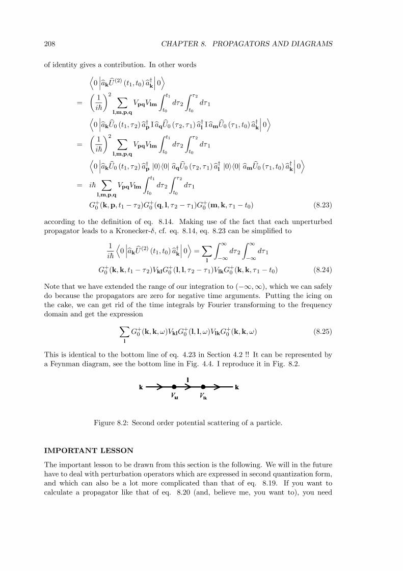
208 CHAPTER 8. PROPAGATORS AND DIAGRAMS
of identity gives a contribution. In other wordsD0¯bak bU (2) (t1, t0)ba†k ¯ 0E
=
µ1
i~
¶2 Xl,m,p,q
VpqVlm
Z t1
t0
dτ2
Z τ2
t0
dτ1D0¯bak bU0 (t1, τ2)ba†p Ibaq bU0 (τ2, τ1)ba†l Ibam bU0 (τ1, t0)ba†k ¯ 0E
=
µ1
i~
¶2 Xl,m,p,q
VpqVlm
Z t1
t0
dτ2
Z τ2
t0
dτ1D0¯bak bU0 (t1, τ2)ba†p |0ih0| baq bU0 (τ2, τ1)ba†l |0ih0| bam bU0 (τ1, t0)ba†k ¯ 0E
= i~X
l,m,p,q
VpqVlm
Z t1
t0
dτ2
Z τ2
t0
dτ1
G+0 (k,p, t1 − τ2)G+0 (q, l, τ2 − τ1)G
+0 (m,k, τ1 − t0) (8.23)
according to the definition of eq. 8.14. Making use of the fact that each unperturbedpropagator leads to a Kronecker-δ, cf. eq. 8.14, eq. 8.23 can be simplified to
1
i~
D0¯bak bU (2) (t1, t0)ba†k ¯ 0E =X
l
Z ∞
−∞dτ2
Z ∞
−∞dτ1
G+0 (k,k, t1 − τ2)VklG+0 (l, l, τ2 − τ1)VlkG
+0 (k,k, τ1 − t0) (8.24)
Note that we have extended the range of our integration to (−∞,∞), which we can safelydo because the propagators are zero for negative time arguments. Putting the icing onthe cake, we can get rid of the time integrals by Fourier transforming to the frequencydomain and get the expressionX
l
G+0 (k,k,ω)VklG+0 (l, l,ω)VlkG
+0 (k,k,ω) (8.25)
This is identical to the bottom line of eq. 4.23 in Section 4.2 !! It can be represented bya Feynman diagram, see the bottom line in Fig. 4.4. I reproduce it in Fig. 8.2.
klV lkVk k
l
klV lkVk k
l
Figure 8.2: Second order potential scattering of a particle.
IMPORTANT LESSON
The important lesson to be drawn from this section is the following. We will in the futurehave to deal with perturbation operators which are expressed in second quantization form,and which can also be a lot more complicated than that of eq. 8.19. If you want tocalculate a propagator like that of eq. 8.20 (and, believe me, you want to), you need
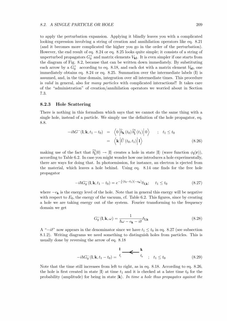
8.2. A SINGLE PARTICLE OR HOLE 209
to apply the perturbation expansion. Applying it blindly leaves you with a complicatedlooking expression involving a string of creation and annihilation operators like eq. 8.21(and it becomes more complicated the higher you go in the order of the perturbation).However, the end result of eq. 8.24 or eq. 8.25 looks quite simple; it consists of a string ofunperturbed propagators G+0 and matrix elements Vkl. It is even simpler if one starts fromthe diagram of Fig. 8.2, because that can be written down immediately. By substitutingeach arrow by a G+0 according to eq. 8.18, and each dot with a matrix element Vkl, oneimmediately obtains eq. 8.24 or eq. 8.25. Summation over the intermediate labels (l) isassumed, and, in the time domain, integration over all intermediate times. This procedureis valid in general, also for many particles with complicated interactions!! It takes careof the “administration” of creation/annihilation operators we worried about in Section7.3.
8.2.3 Hole Scattering
There is nothing in this formalism which says that we cannot do the same thing with asingle hole, instead of a particle. We simply use the definition of the hole propagator, eq.8.8.
−i~G−(l,k, t1 − t0) =D0¯bbk (t0)bb†l (t1)¯ 0E ; t1 ≤ t0
=Dk¯ bU (t0, t1)¯ lE (8.26)
making use of the fact that bb†l |0i → |li creates a hole in state |li (wave function φl(r)),according to Table 6.2. In case you might wonder how one introduces a hole experimentally,there are ways for doing that. In photoemission, for instance, an electron is ejected fromthe material, which leaves a hole behind. Using eq. 8.14 one finds for the free holepropagator
−i~G−0 (l,k, t1 − t0) = e−i~ (t0−t1)(−²k)δl,k; t1 ≤ t0 (8.27)
where −²k is the energy level of the hole. Note that in general this energy will be negativewith respect to E0, the energy of the vacuum, cf. Table 6.2. This figures, since by creatinga hole we are taking energy out of the system. Fourier transforming to the frequencydomain we get
G−0 (l,k,ω) =1
~ω − ²k − iδ δl,k (8.28)
A “−iδ” now appears in the denominator since we have t1 ≤ t0 in eq. 8.27 (see subsection8.1.2). Writing diagrams we need something to distinguish holes from particles. This isusually done by reversing the arrow of eq. 8.18
−i~G−0 (l,k, t1 − t0) = 0tk
1tl
; t1 ≤ t0 (8.29)
Note that the time still increases from left to right, as in eq. 8.18. According to eq. 8.26,the hole is first created in state |li at time t1 and it is checked at a later time t0 for theprobability (amplitude) for being in state |ki. In time a hole thus propagates against the
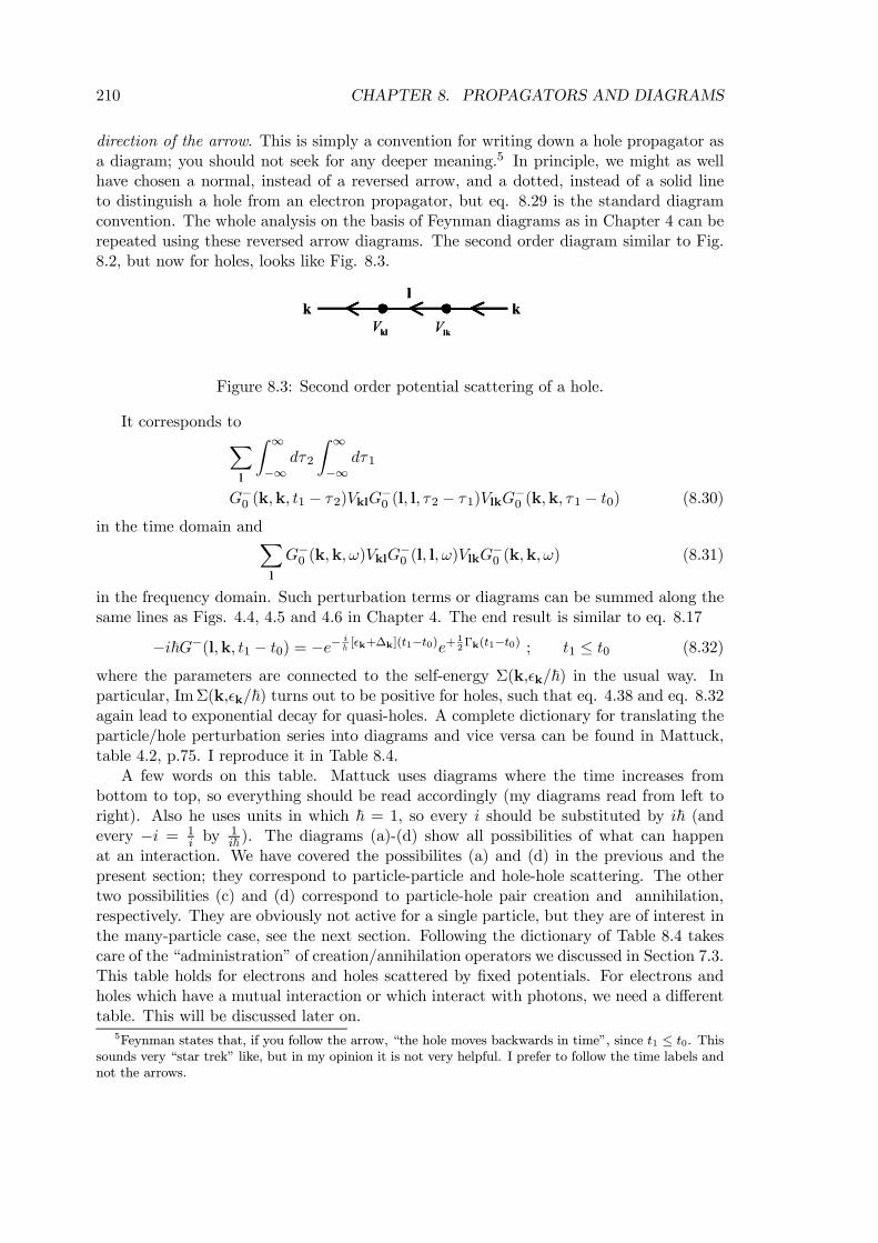
210 CHAPTER 8. PROPAGATORS AND DIAGRAMS
direction of the arrow. This is simply a convention for writing down a hole propagator asa diagram; you should not seek for any deeper meaning.5 In principle, we might as wellhave chosen a normal, instead of a reversed arrow, and a dotted, instead of a solid lineto distinguish a hole from an electron propagator, but eq. 8.29 is the standard diagramconvention. The whole analysis on the basis of Feynman diagrams as in Chapter 4 can berepeated using these reversed arrow diagrams. The second order diagram similar to Fig.8.2, but now for holes, looks like Fig. 8.3.
klV lkVk k
l
klV lkVk k
l
Figure 8.3: Second order potential scattering of a hole.
It corresponds toXl
Z ∞
−∞dτ2
Z ∞
−∞dτ1
G−0 (k,k, t1 − τ2)VklG−0 (l, l, τ2 − τ1)VlkG
−0 (k,k, τ1 − t0) (8.30)
in the time domain andXl
G−0 (k,k,ω)VklG−0 (l, l,ω)VlkG
−0 (k,k,ω) (8.31)
in the frequency domain. Such perturbation terms or diagrams can be summed along thesame lines as Figs. 4.4, 4.5 and 4.6 in Chapter 4. The end result is similar to eq. 8.17
−i~G−(l,k, t1 − t0) = −e− i~ [²k+∆k](t1−t0)e+
12Γk(t1−t0) ; t1 ≤ t0 (8.32)
where the parameters are connected to the self-energy Σ(k,²k/~) in the usual way. Inparticular, ImΣ(k,²k/~) turns out to be positive for holes, such that eq. 4.38 and eq. 8.32again lead to exponential decay for quasi-holes. A complete dictionary for translating theparticle/hole perturbation series into diagrams and vice versa can be found in Mattuck,table 4.2, p.75. I reproduce it in Table 8.4.
A few words on this table. Mattuck uses diagrams where the time increases frombottom to top, so everything should be read accordingly (my diagrams read from left toright). Also he uses units in which ~ = 1, so every i should be substituted by i~ (andevery −i = 1
i by1i~ ). The diagrams (a)-(d) show all possibilities of what can happen
at an interaction. We have covered the possibilites (a) and (d) in the previous and thepresent section; they correspond to particle-particle and hole-hole scattering. The othertwo possibilities (c) and (d) correspond to particle-hole pair creation and annihilation,respectively. They are obviously not active for a single particle, but they are of interest inthe many-particle case, see the next section. Following the dictionary of Table 8.4 takescare of the “administration” of creation/annihilation operators we discussed in Section 7.3.This table holds for electrons and holes scattered by fixed potentials. For electrons andholes which have a mutual interaction or which interact with photons, we need a differenttable. This will be discussed later on.
5Feynman states that, if you follow the arrow, “the hole moves backwards in time”, since t1 ≤ t0. Thissounds very “star trek” like, but in my opinion it is not very helpful. I prefer to follow the time labels andnot the arrows.
8.3. MANY PARTICLES AND HOLES 211
Figure 8.4: Mattuck’s table 4.2, p.75
8.3 Many Particles and Holes
The next step up in complexity is a many-particle system of non-interacting particles (andholes) as in Section 6.3.1. As one might expect, the homogeneous electron gas is our toymodel for that situation. The Hamiltonian according to eq. 6.51 is given by
bh = E0 − X|k|≤kF
²kbb†kbbk + X|k|>kF
²kba†kbak (8.33)
It is possible to study scattering in such a system by introducing atomic scattering poten-tials. These give a perturbation of the type we have seen before
bV =Xk,l
Vklbc†kbcl=
X|k|>kF ,|l|>kF
Vklba†kbal + X|k|>kF ,|l|≤kF
Vklba†kbb†l+
X|k|≤kF ,|l|>kF
Vklbbkbal + X|k|≤kF ,|l|≤kF
Vklbbkbb†l (8.34)
where bck and bc†k are general fermion operators, which can be substituted by particle/holeoperators according to the familiar rules. Again one is interested in the result of the
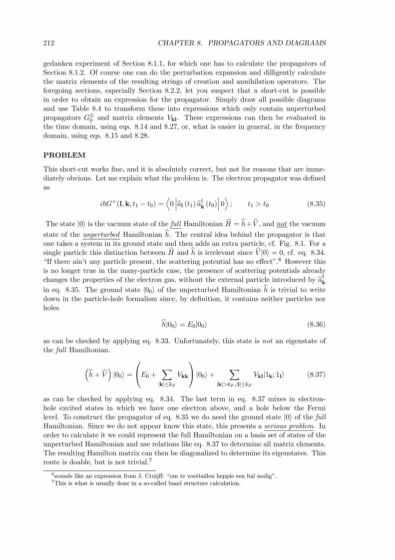
212 CHAPTER 8. PROPAGATORS AND DIAGRAMS
gedanken experiment of Section 8.1.1, for which one has to calculate the propagators ofSection 8.1.2. Of course one can do the perturbation expansion and dilligently calculatethe matrix elements of the resulting strings of creation and annihilation operators. Theforegoing sections, especially Section 8.2.2, let you suspect that a short-cut is possiblein order to obtain an expression for the propagator. Simply draw all possible diagramsand use Table 8.4 to transform these into expressions which only contain unperturbedpropagators G±0 and matrix elements Vkl. These expressions can then be evaluated inthe time domain, using eqs. 8.14 and 8.27, or, what is easier in general, in the frequencydomain, using eqs. 8.15 and 8.28.
PROBLEM
This short-cut works fine, and it is absolutely correct, but not for reasons that are imme-diately obvious. Let me explain what the problem is. The electron propagator was definedas
i~G+(l,k, t1 − t0) =D0¯bal (t1)ba†k (t0)¯ 0E ; t1 > t0 (8.35)
The state |0i is the vacuum state of the full Hamiltonian bH = bh+ bV , and not the vacuumstate of the unperturbed Hamiltonian bh. The central idea behind the propagator is thatone takes a system in its ground state and then adds an extra particle, cf. Fig. 8.1. For asingle particle this distinction between bH and bh is irrelevant since bV |0i = 0, cf. eq. 8.34.“If there ain’t any particle present, the scattering potential has no effect”.6 However thisis no longer true in the many-particle case, the presence of scattering potentials alreadychanges the properties of the electron gas, without the external particle introduced by ba†kin eq. 8.35. The ground state |00i of the unperturbed Hamiltonian bh is trivial to writedown in the particle-hole formalism since, by definition, it contains neither particles norholes
bh|00i = E0|00i (8.36)
as can be checked by applying eq. 8.33. Unfortunately, this state is not an eigenstate ofthe full Hamiltonian.
³bh+ bV ´ |00i =E0 + X
|k|≤kFVkk
|00i+ X|k|>kF ,|l|≤kF
Vkl|1k; 1li (8.37)
as can be checked by applying eq. 8.34. The last term in eq. 8.37 mixes in electron-hole excited states in which we have one electron above, and a hole below the Fermilevel. To construct the propagator of eq. 8.35 we do need the ground state |0i of the fullHamiltonian. Since we do not appear know this state, this presents a serious problem. Inorder to calculate it we could represent the full Hamiltonian on a basis set of states of theunperturbed Hamiltonian and use relations like eq. 8.37 to determine all matrix elements.The resulting Hamilton matrix can then be diagonalized to determine its eigenstates. Thisroute is doable, but is not trivial.7
6sounds like an expression from J. Cruijff: “om te voetballen heppie een bal nodig”.7This is what is usually done in a so-called band structure calculation.
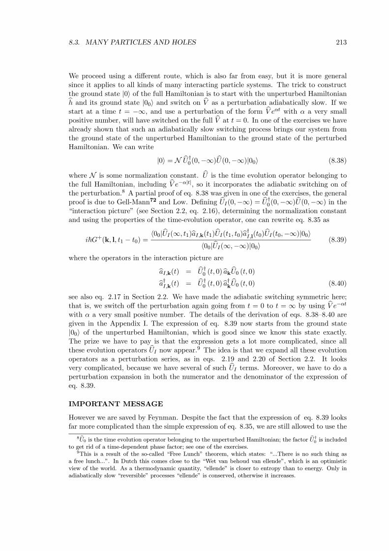
8.3. MANY PARTICLES AND HOLES 213
We proceed using a different route, which is also far from easy, but it is more generalsince it applies to all kinds of many interacting particle systems. The trick to constructthe ground state |0i of the full Hamiltonian is to start with the unperturbed Hamiltonianbh and its ground state |00i and switch on bV as a perturbation adiabatically slow. If westart at a time t = −∞, and use a perturbation of the form bV eαt with α a very smallpositive number, will have switched on the full bV at t = 0. In one of the exercises we havealready shown that such an adiabatically slow switching process brings our system fromthe ground state of the unperturbed Hamiltonian to the ground state of the perturbedHamiltonian. We can write
|0i = N bU †0(0,−∞)bU(0,−∞)|00i (8.38)
where N is some normalization constant. bU is the time evolution operator belonging tothe full Hamiltonian, including bV e−α|t|, so it incorporates the adiabatic switching on ofthe perturbation.8 A partial proof of eq. 8.38 was given in one of the exercises, the generalproof is due to Gell-Mann72 and Low. Defining bUI(0,−∞) = bU †0(0,−∞)bU(0,−∞) in the“interaction picture” (see Section 2.2, eq. 2.16), determining the normalization constantand using the properties of the time-evolution operator, one can rewrite eq. 8.35 as
i~G+(k, l, t1 − t0) =h00|bUI(∞, t1)baI,k(t1)bUI(t1, t0)ba†I,l(t0)bUI(t0,−∞)|00i
h00|bUI(∞,−∞)|00i (8.39)
where the operators in the interaction picture are
baI,k(t) = bU †0 (t, 0)bak bU0 (t, 0)ba†I,k(t) = bU †0 (t, 0)ba†k bU0 (t, 0) (8.40)
see also eq. 2.17 in Section 2.2. We have made the adiabatic switching symmetric here;that is, we switch off the perturbation again going from t = 0 to t = ∞ by using bV e−αtwith α a very small positive number. The details of the derivation of eqs. 8.38—8.40 aregiven in the Appendix I. The expression of eq. 8.39 now starts from the ground state|00i of the unperturbed Hamiltonian, which is good since we know this state exactly.The prize we have to pay is that the expression gets a lot more complicated, since allthese evolution operators bUI now appear.9 The idea is that we expand all these evolutionoperators as a perturbation series, as in eqs. 2.19 and 2.20 of Section 2.2. It looksvery complicated, because we have several of such bUI terms. Moreover, we have to do aperturbation expansion in both the numerator and the denominator of the expression ofeq. 8.39.
IMPORTANT MESSAGE
However we are saved by Feynman. Despite the fact that the expression of eq. 8.39 looksfar more complicated than the simple expression of eq. 8.35, we are still allowed to use the
8 bU0 is the time evolution operator belonging to the unperturbed Hamiltonian; the factor bU†0 is includedto get rid of a time-dependent phase factor; see one of the exercises.
9This is a result of the so-called “Free Lunch” theorem, which states: “...There is no such thing asa free lunch...”. In Dutch this comes close to the “Wet van behoud van ellende”, which is an optimisticview of the world. As a thermodynamic quantity, “ellende” is closer to entropy than to energy. Only inadiabatically slow “reversible” processes “ellende” is conserved, otherwise it increases.
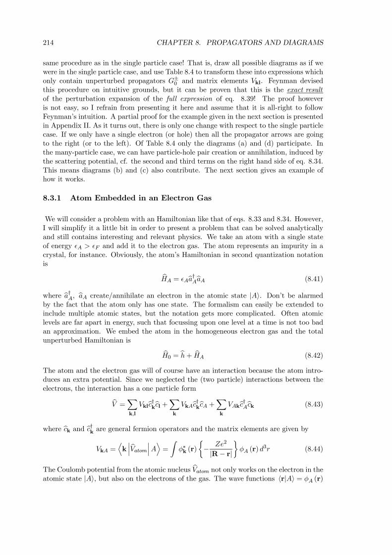
214 CHAPTER 8. PROPAGATORS AND DIAGRAMS
same procedure as in the single particle case! That is, draw all possible diagrams as if wewere in the single particle case, and use Table 8.4 to transform these into expressions whichonly contain unperturbed propagators G±0 and matrix elements Vkl. Feynman devisedthis procedure on intuitive grounds, but it can be proven that this is the exact resultof the perturbation expansion of the full expression of eq. 8.39! The proof howeveris not easy, so I refrain from presenting it here and assume that it is all-right to followFeynman’s intuition. A partial proof for the example given in the next section is presentedin Appendix II. As it turns out, there is only one change with respect to the single particlecase. If we only have a single electron (or hole) then all the propagator arrows are goingto the right (or to the left). Of Table 8.4 only the diagrams (a) and (d) participate. Inthe many-particle case, we can have particle-hole pair creation or annihilation, induced bythe scattering potential, cf. the second and third terms on the right hand side of eq. 8.34.This means diagrams (b) and (c) also contribute. The next section gives an example ofhow it works.
8.3.1 Atom Embedded in an Electron Gas
We will consider a problem with an Hamiltonian like that of eqs. 8.33 and 8.34. However,I will simplify it a little bit in order to present a problem that can be solved analyticallyand still contains interesting and relevant physics. We take an atom with a single stateof energy ²A > ²F and add it to the electron gas. The atom represents an impurity in acrystal, for instance. Obviously, the atom’s Hamiltonian in second quantization notationis bHA = ²Aba†AbaA (8.41)
where ba†A, baA create/annihilate an electron in the atomic state |Ai. Don’t be alarmedby the fact that the atom only has one state. The formalism can easily be extended toinclude multiple atomic states, but the notation gets more complicated. Often atomiclevels are far apart in energy, such that focussing upon one level at a time is not too badan approximation. We embed the atom in the homogeneous electron gas and the totalunperturbed Hamiltonian is bH0 = bh+ bHA (8.42)
The atom and the electron gas will of course have an interaction because the atom intro-duces an extra potential. Since we neglected the (two particle) interactions between theelectrons, the interaction has a one particle form
bV =Xk,l
Vklbc†kbcl +Xk
VkAbc†kbcA +Xk
VAkbc†Abck (8.43)
where bck and bc†k are general fermion operators and the matrix elements are given byVkA =
Dk¯ bVatom ¯AE = Z φ∗k (r)
½− Ze2
|R− r|¾φA (r) d
3r (8.44)
The Coulomb potential from the atomic nucleus bVatom not only works on the electron in theatomic state |Ai, but also on the electrons of the gas. The wave functions hr|Ai = φA (r)
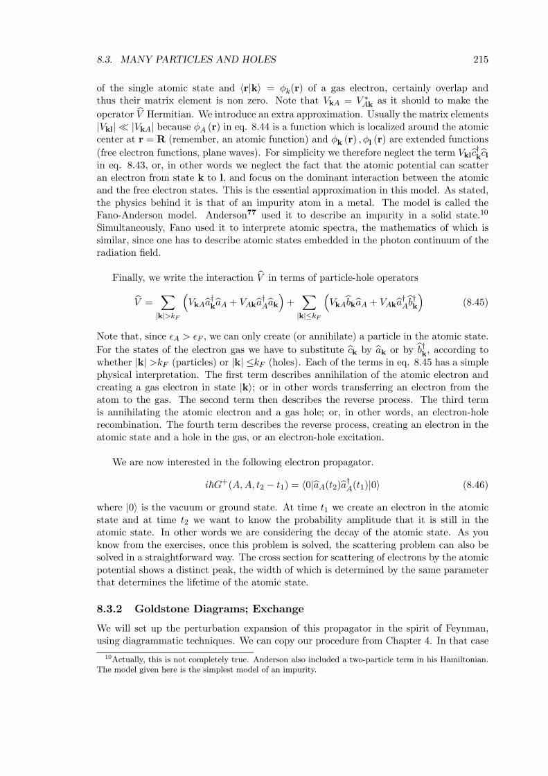
8.3. MANY PARTICLES AND HOLES 215
of the single atomic state and hr|ki = φk(r) of a gas electron, certainly overlap andthus their matrix element is non zero. Note that VkA = V ∗Ak as it should to make theoperator bV Hermitian. We introduce an extra approximation. Usually the matrix elements|Vkl| ¿ |VkA| because φA (r) in eq. 8.44 is a function which is localized around the atomiccenter at r = R (remember, an atomic function) and φk (r) ,φl (r) are extended functions
(free electron functions, plane waves). For simplicity we therefore neglect the term Vklbc†kbclin eq. 8.43, or, in other words we neglect the fact that the atomic potential can scatteran electron from state k to l, and focus on the dominant interaction between the atomicand the free electron states. This is the essential approximation in this model. As stated,the physics behind it is that of an impurity atom in a metal. The model is called theFano-Anderson model. Anderson77 used it to describe an impurity in a solid state.10
Simultaneously, Fano used it to interprete atomic spectra, the mathematics of which issimilar, since one has to describe atomic states embedded in the photon continuum of theradiation field.
Finally, we write the interaction bV in terms of particle-hole operators
bV = X|k|>kF
³VkAba†kbaA + VAkba†Abak´+ X
|k|≤kF
³VkAbbkbaA + VAkba†Abb†k´ (8.45)
Note that, since ²A > ²F , we can only create (or annihilate) a particle in the atomic state.
For the states of the electron gas we have to substitute bck by bak or by bb†k, according towhether |k| >kF (particles) or |k| ≤kF (holes). Each of the terms in eq. 8.45 has a simplephysical interpretation. The first term describes annihilation of the atomic electron andcreating a gas electron in state |ki; or in other words transferring an electron from theatom to the gas. The second term then describes the reverse process. The third termis annihilating the atomic electron and a gas hole; or, in other words, an electron-holerecombination. The fourth term describes the reverse process, creating an electron in theatomic state and a hole in the gas, or an electron-hole excitation.
We are now interested in the following electron propagator.
i~G+(A,A, t2 − t1) = h0|baA(t2)ba†A(t1)|0i (8.46)
where |0i is the vacuum or ground state. At time t1 we create an electron in the atomicstate and at time t2 we want to know the probability amplitude that it is still in theatomic state. In other words we are considering the decay of the atomic state. As youknow from the exercises, once this problem is solved, the scattering problem can also besolved in a straightforward way. The cross section for scattering of electrons by the atomicpotential shows a distinct peak, the width of which is determined by the same parameterthat determines the lifetime of the atomic state.
8.3.2 Goldstone Diagrams; Exchange
We will set up the perturbation expansion of this propagator in the spirit of Feynman,using diagrammatic techniques. We can copy our procedure from Chapter 4. In that case
10Actually, this is not completely true. Anderson also included a two-particle term in his Hamiltonian.The model given here is the simplest model of an impurity.
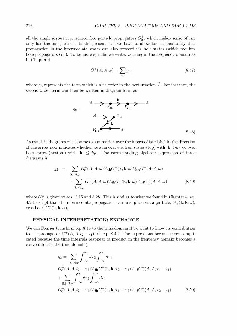
216 CHAPTER 8. PROPAGATORS AND DIAGRAMS
all the single arrows represented free particle propagators G+0 , which makes sense of oneonly has the one particle. In the present case we have to allow for the possibility thatpropagation in the intermediate states can also proceed via hole states (which requireshole propagators G−0 ). To be more specific we write, working in the frequency domain asin Chapter 4
G+(A,A,ω) =Xn
gn (8.47)
where gn represents the term which is n’th order in the perturbation bV . For instance, thesecond order term can then be written in diagram form as
g2 =
A Ak
k,AV AV ,k
+
A k,AV
AV ,k
kA
(8.48)
As usual, in diagrams one assumes a summation over the intermediate label k; the directionof the arrow now indicates whether we sum over electron states (top) with |k| >kF or overhole states (bottom) with |k| ≤ kF . The corresponding algebraic expression of thesediagrams is
g2 =X|k|>kF
G+0 (A,A,ω)VAkG+0 (k,k,ω)VkAG
+0 (A,A,ω)
+X|k|≤kF
G+0 (A,A,ω)VAkG−0 (k,k,ω)VkAG
+0 (A,A,ω) (8.49)
where G±0 is given by eqs. 8.15 and 8.28. This is similar to what we found in Chapter 4, eq.4.23, except that the intermediate propagation can take place via a particle, G+0 (k,k,ω),or a hole, G−0 (k,k,ω).
PHYSICAL INTERPRETATION; EXCHANGE
We can Fourier transform eq. 8.49 to the time domain if we want to know its contributionto the propagator G+(A,A, t2 − t1) of eq. 8.46. The expressions become more compli-cated because the time integrals reappear (a product in the frequency domain becomes aconvolution in the time domain).
g2 =X|k|>kF
Z ∞
−∞dτ2
Z ∞
−∞dτ1
G+0 (A,A, t2 − τ2)VAkG+0 (k,k, τ2 − τ1)VkAG
+0 (A,A, τ1 − t1)
+X|k|≤kF
Z ∞
−∞dτ2
Z ∞
−∞dτ1
G+0 (A,A, t2 − τ1)VAkG−0 (k,k, τ1 − τ2)VkAG
+0 (A,A, τ2 − t1) (8.50)
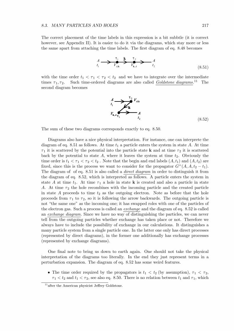
8.3. MANY PARTICLES AND HOLES 217
The correct placement of the time labels in this expression is a bit subbtle (it is correcthowever, see Appendix II). It is easier to do it via the diagrams, which stay more or lessthe same apart from attaching the time labels. The first diagram of eq. 8.48 becomes
A Ak
k,AV AV ,k1t 2t1τ 2τ
(8.51)
with the time order t1 < τ1 < τ2 < t2 and we have to integrate over the intermediatetimes τ1, τ2. Such time-ordered diagrams are also called Goldstone diagrams.11 Thesecond diagram becomes
A k,AV
AV ,k
kA
1t
2t1τ
2τA k,AV
AV ,k
kA
A k,AV
AV ,k
kA
1t
2t1τ
2τ
(8.52)
The sum of these two diagrams corresponds exactly to eq. 8.50.
Diagrams also have a nice physical interpretation. For instance, one can interprete thediagram of eq. 8.51 as follows. At time t1 a particle enters the system in state A. At timeτ1 it is scattered by the potential into the particle state k and at time τ2 it is scatteredback by the potential to state A, where it leaves the system at time t2. Obviously thetime order is t1 < τ1 < τ2 < t2 . Note that the begin and end labels (A, t1) and (A, t2) arefixed, since this is the process we want to consider for the propagator G+(A,A, t2 − t1).The diagram of of eq. 8.51 is also called a direct diagram in order to distinguish it fromthe diagram of eq. 8.52, which is interpreted as follows. A particle enters the system instate A at time t1. At time τ1 a hole in state k is created and also a particle in stateA. At time τ2 the hole recombines with the incoming particle and the created particlein state A proceeds to time t2 as the outgoing electron. Note as before that the holeproceeds from τ1 to τ2, so it is following the arrow backwards. The outgoing particle isnot “the same one” as the incoming one; it has swapped roles with one of the particles ofthe electron gas. Such a process is called an exchange and the diagram of eq. 8.52 is calledan exchange diagram. Since we have no way of distinguishing the particles, we can nevertell from the outgoing particles whether exchange has taken place or not. Therefore wealways have to include the possibility of exchange in our calculations. It distinguishes amany particle system from a single particle one. In the latter one only has direct processes(represented by direct diagrams), in the former one additionally has exchange processes(represented by exchange diagrams).
One final note to bring us down to earth again. One should not take the physicalinterpretation of the diagrams too literally. In the end they just represent terms in aperturbation expansion. The diagram of eq. 8.52 has some weird features.
• The time order required by the propagators is t1 < t2 (by assumption), τ1 < τ2,τ1 < t2 and t1 < τ2, see also eq. 8.50. There is no relation between t1 and τ1, which
11after the American physicist Jeffrey Goldstone.
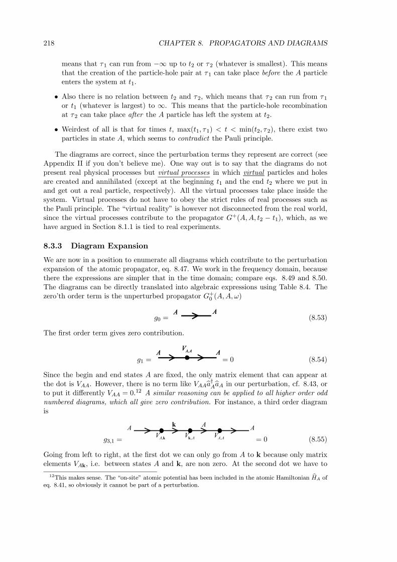
218 CHAPTER 8. PROPAGATORS AND DIAGRAMS
means that τ1 can run from −∞ up to t2 or τ2 (whatever is smallest). This meansthat the creation of the particle-hole pair at τ1 can take place before the A particleenters the system at t1.
• Also there is no relation between t2 and τ2, which means that τ2 can run from τ1or t1 (whatever is largest) to ∞. This means that the particle-hole recombinationat τ2 can take place after the A particle has left the system at t2.
• Weirdest of all is that for times t, max(t1, τ1) < t < min(t2, τ2), there exist twoparticles in state A, which seems to contradict the Pauli principle.
The diagrams are correct, since the perturbation terms they represent are correct (seeAppendix II if you don’t believe me). One way out is to say that the diagrams do notpresent real physical processes but virtual processes in which virtual particles and holesare created and annihilated (except at the beginning t1 and the end t2 where we put inand get out a real particle, respectively). All the virtual processes take place inside thesystem. Virtual processes do not have to obey the strict rules of real processes such asthe Pauli principle. The “virtual reality” is however not disconnected from the real world,since the virtual processes contribute to the propagator G+(A,A, t2 − t1), which, as wehave argued in Section 8.1.1 is tied to real experiments.
8.3.3 Diagram Expansion
We are now in a position to enumerate all diagrams which contribute to the perturbationexpansion of the atomic propagator, eq. 8.47. We work in the frequency domain, becausethere the expressions are simpler that in the time domain; compare eqs. 8.49 and 8.50.The diagrams can be directly translated into algebraic expressions using Table 8.4. Thezero’th order term is the unperturbed propagator G+0 (A,A,ω)
g0 =A AA A
(8.53)
The first order term gives zero contribution.
g1 =AA ,A AV AA ,A AV= 0 (8.54)
Since the begin and end states A are fixed, the only matrix element that can appear atthe dot is VAA. However, there is no term like VAAba†AbaA in our perturbation, cf. 8.43, orto put it differently VAA = 0.
12 A similar reasoning can be applied to all higher order oddnumbered diagrams, which all give zero contribution. For instance, a third order diagramis
g3,1 =
A Ak
k,AV AV ,k AAV ,
A
= 0 (8.55)
Going from left to right, at the first dot we can only go from A to k because only matrixelements VAk, i.e. between states A and k, are non zero. At the second dot we have to
12This makes sense. The “on-site” atomic potential has been included in the atomic Hamiltonian bHA ofeq. 8.41, so obviously it cannot be part of a perturbation.
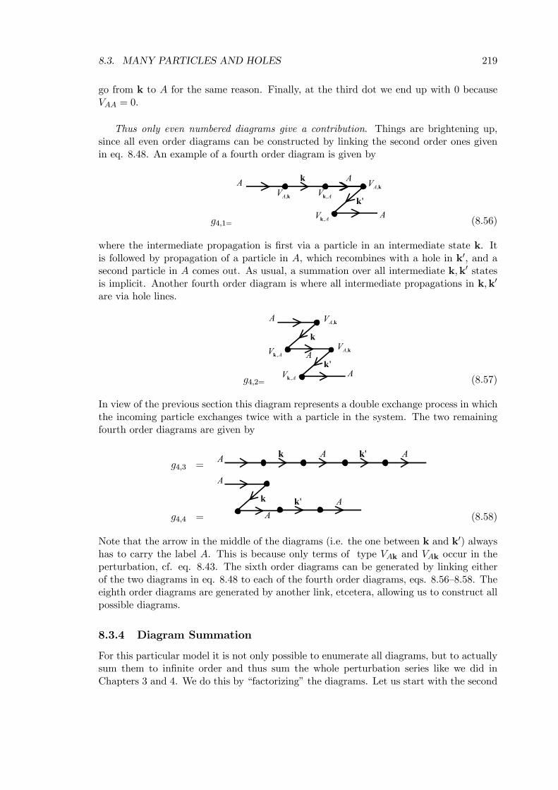
8.3. MANY PARTICLES AND HOLES 219
go from k to A for the same reason. Finally, at the third dot we end up with 0 becauseVAA = 0.
Thus only even numbered diagrams give a contribution. Things are brightening up,since all even order diagrams can be constructed by linking the second order ones givenin eq. 8.48. An example of a fourth order diagram is given by
g4,1=
k,AVA k
k,AV AV ,k
A
AV ,k
'kA
(8.56)
where the intermediate propagation is first via a particle in an intermediate state k. Itis followed by propagation of a particle in A, which recombines with a hole in k0, and asecond particle in A comes out. As usual, a summation over all intermediate k,k0 statesis implicit. Another fourth order diagram is where all intermediate propagations in k,k0
are via hole lines.
g4,2=
A k,AV
AV ,k
k
A
k,AV
'kAV ,k
A
(8.57)
In view of the previous section this diagram represents a double exchange process in whichthe incoming particle exchanges twice with a particle in the system. The two remainingfourth order diagrams are given by
g4,3 =A'kAkA
g4,4 =
k
A
A
A'k(8.58)
Note that the arrow in the middle of the diagrams (i.e. the one between k and k0) alwayshas to carry the label A. This is because only terms of type VAk and VAk occur in theperturbation, cf. eq. 8.43. The sixth order diagrams can be generated by linking eitherof the two diagrams in eq. 8.48 to each of the fourth order diagrams, eqs. 8.56—8.58. Theeighth order diagrams are generated by another link, etcetera, allowing us to construct allpossible diagrams.
8.3.4 Diagram Summation
For this particular model it is not only possible to enumerate all diagrams, but to actuallysum them to infinite order and thus sum the whole perturbation series like we did inChapters 3 and 4. We do this by “factorizing” the diagrams. Let us start with the second
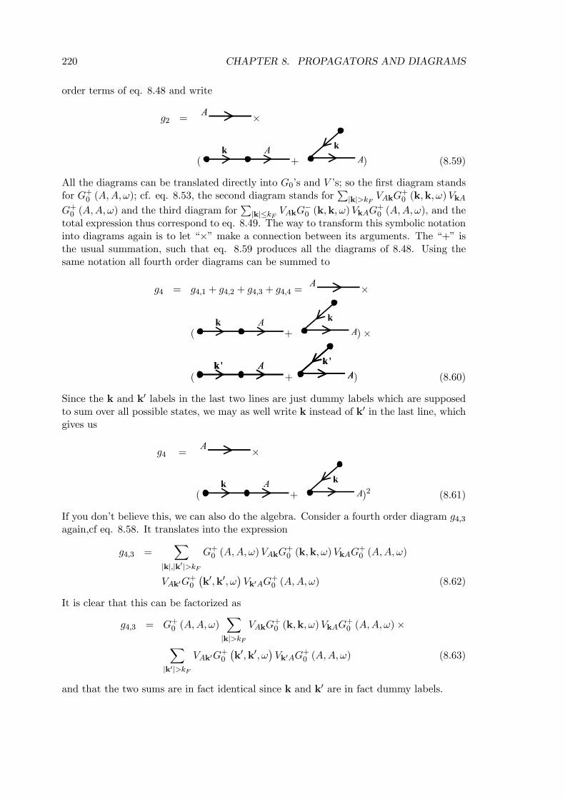
220 CHAPTER 8. PROPAGATORS AND DIAGRAMS
order terms of eq. 8.48 and write
g2 =A ×
(Ak
+
kA) (8.59)
All the diagrams can be translated directly into G0’s and V ’s; so the first diagram standsfor G+0 (A,A,ω); cf. eq. 8.53, the second diagram stands for
P|k|>kF VAkG
+0 (k,k,ω)VkA
G+0 (A,A,ω) and the third diagram forP|k|≤kF VAkG
−0 (k,k,ω)VkAG
+0 (A,A,ω), and the
total expression thus correspond to eq. 8.49. The way to transform this symbolic notationinto diagrams again is to let “×” make a connection between its arguments. The “+” isthe usual summation, such that eq. 8.59 produces all the diagrams of 8.48. Using thesame notation all fourth order diagrams can be summed to
g4 = g4,1 + g4,2 + g4,3 + g4,4 =A ×
(Ak
+
kA)×
(A'k A'k
+
'kA
'kA) (8.60)
Since the k and k0 labels in the last two lines are just dummy labels which are supposedto sum over all possible states, we may as well write k instead of k0 in the last line, whichgives us
g4 =A ×
(Ak
+
kA)2 (8.61)
If you don’t believe this, we can also do the algebra. Consider a fourth order diagram g4,3again,cf eq. 8.58. It translates into the expression
g4,3 =X
|k|,|k0|>kFG+0 (A,A,ω)VAkG
+0 (k,k,ω)VkAG
+0 (A,A,ω)
VAk0G+0
¡k0,k0,ω
¢Vk0AG
+0 (A,A,ω) (8.62)
It is clear that this can be factorized as
g4,3 = G+0 (A,A,ω)X|k|>kF
VAkG+0 (k,k,ω)VkAG
+0 (A,A,ω)×X
|k0|>kFVAk0G
+0
¡k0,k0,ω
¢Vk0AG
+0 (A,A,ω) (8.63)
and that the two sums are in fact identical since k and k0 are in fact dummy labels.
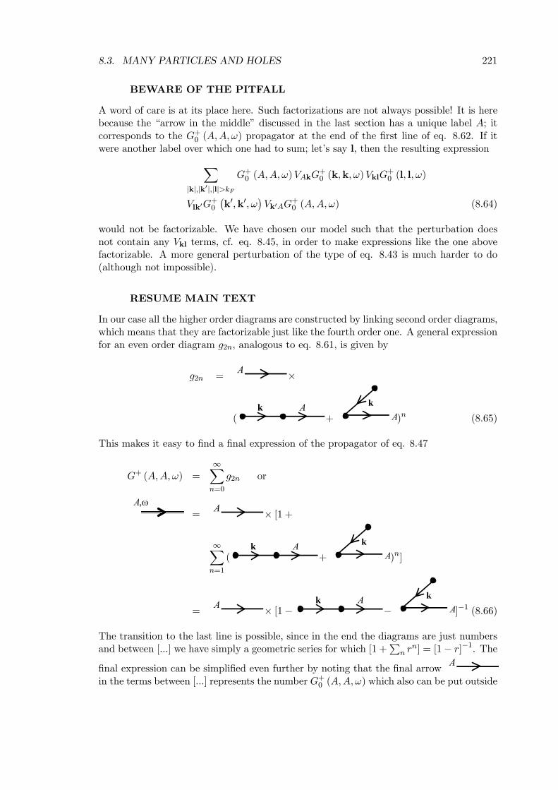
8.3. MANY PARTICLES AND HOLES 221
BEWARE OF THE PITFALL
A word of care is at its place here. Such factorizations are not always possible! It is herebecause the “arrow in the middle” discussed in the last section has a unique label A; itcorresponds to the G+0 (A,A,ω) propagator at the end of the first line of eq. 8.62. If itwere another label over which one had to sum; let’s say l, then the resulting expressionX
|k|,|k0|,|l|>kFG+0 (A,A,ω)VAkG
+0 (k,k,ω)VklG
+0 (l, l,ω)
Vlk0G+0
¡k0,k0,ω
¢Vk0AG
+0 (A,A,ω) (8.64)
would not be factorizable. We have chosen our model such that the perturbation doesnot contain any Vkl terms, cf. eq. 8.45, in order to make expressions like the one abovefactorizable. A more general perturbation of the type of eq. 8.43 is much harder to do(although not impossible).
RESUME MAIN TEXT
In our case all the higher order diagrams are constructed by linking second order diagrams,which means that they are factorizable just like the fourth order one. A general expressionfor an even order diagram g2n, analogous to eq. 8.61, is given by
g2n =A ×
(Ak
+
kA)n (8.65)
This makes it easy to find a final expression of the propagator of eq. 8.47
G+ (A,A,ω) =∞Xn=0
g2n or
ω,A=
A × [1 +
∞Xn=1
(Ak
+
kA)n]
=A × [1−
Ak−
kA]−1 (8.66)
The transition to the last line is possible, since in the end the diagrams are just numbersand between [...] we have simply a geometric series for which [1 +
Pn r
n] = [1− r]−1. Thefinal expression can be simplified even further by noting that the final arrow
A
in the terms between [...] represents the number G+0 (A,A,ω) which also can be put outside
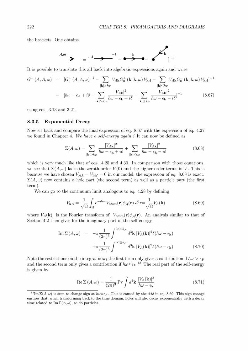
222 CHAPTER 8. PROPAGATORS AND DIAGRAMS
the brackets. One obtains
ω,A= [
A −1−
k−
k]−1
It is possible to translate this all back into algebraic expressions again and write
G+ (A,A,ω) = [G+0 (A,A,ω)−1 −
X|k|>kF
VAkG+0 (k,k,ω)VkA −
X|k|≤kF
VAkG−0 (k,k,ω)VkA]
−1
= [~ω − ²A + iδ −X|k|>kF
|VAk|2~ω − ²k + iδ −
X|k|≤kF
|VAk|2~ω − ²k − iδ ]
−1 (8.67)
using eqs. 3.13 and 3.21.
8.3.5 Exponential Decay
Now sit back and compare the final expression of eq. 8.67 with the expression of eq. 4.27we found in Chapter 4. We have a self-energy again ! It can now be defined as
Σ(A,ω) =X|k|>kF
|VAk|2~ω − ²k + iδ +
X|k|≤kF
|VAk|2~ω − ²k − iδ (8.68)
which is very much like that of eqs. 4.25 and 4.30. In comparison with those equations,we see that Σ(A,ω) lacks the zeroth order V (0) and the higher order terms in V . This isbecause we have chosen VAA = Vkk0 = 0 in our model; the expression of eq. 8.68 is exact.Σ(A,ω) now contains a hole part (the second term) as well as a particle part (the firstterm).
We can go to the continuum limit analogous to eq. 4.28 by defining
VkA =1√Ω
ZΩe−ik·rVatom(r)φA(r) d
3r=1√ΩVA(k) (8.69)
where VA(k) is the Fourier transform of Vatom(r)φA(r). An analysis similar to that ofSection 4.2 then gives for the imaginary part of the self-energy
ImΣ (A,ω) = −π 1
(2π)3
Z |k|>kFd3k |VA(k)|2δ(~ω − ²k)
+π1
(2π)3
Z |k|≤kFd3k |VA(k)|2δ(~ω − ²k) (8.70)
Note the restrictions on the integral now; the first term only gives a contribution if ~ω > ²Fand the second term only gives a contribution if ~ω≤²F .13 The real part of the self-energyis given by
ReΣ (A,ω) =1
(2π)3Pv
Zd3k
|VA(k)|2~ω − ²k (8.71)
13ImΣ(A,ω) is seen to change sign at ~ω=²F . This is caused by the ±iδ in eq. 8.69. This sign changeensures that, when transforming back to the time domain, holes will also decay exponentially with a decaytime related to ImΣ(A,ω), as do particles.
8.4. INTERACTING PARTICLES AND HOLES 223
where Pv indicates a principal value integral. Having defined the self-energy, the propa-gator of eq. 8.67 now simply becomes
G+ (A,A,ω) =1
~ω − ²A − Σ(A,ω) (8.72)
where we got rid of the +iδ because the self-energy is complex anyhow. This equationis similar to eq. 4.27. We now follow Section 4.4 by the letter. Fourier transforming theresult back to the time domain, we obtain
i~G+ (A,A, t2 − t1) =D0¯baA(t2)ba†A(t1)¯ 0E
= zAe− i~ [²A+∆A](t2−t1)e−
12ΓA(t2−t1) for t2 > t1 (8.73)
with
zA =
µ1− 1
~∂ReΣ (A,ω)
∂ω|ω=²A/~
¶−1∆A = ReΣ (A, ²A/~)
ΓA = −2zA~ImΣ (A, ²A/~) (8.74)
So after a long story we are back to a situation that can be described in terms of a levelshift ∆A and a lifetime τA = Γ
−1A , both of which can be derived from the self-energy. The
weight factor zA is in general not equal to 1 anymore, like it was in the single particlecase. One can prove that 0 ≤ zA ≤ 1; the stronger the scattering, the smaller it is;usually it is much closer to 1 however. The appearence of a weight factor is another thingthat distinguishes the many particle from the single particle case. Not surprisingly, eq.8.73 is said to describe the time evolution of a quasi-particle. It has much more of a“quasi” character than in Chapter 4, because we have incorporated all possible exchangeprocesses with particles in the electron gas, as explained in Section 8.3.2. So although weare never sure which particular particle we are looking at, we still can “quasi” do as if weare handling a single particle, and we call it a quasi-particle. Note that because the energy²A > ²F by assumption, it is only the first term of eq. 8.70 that gives a contribution. If²A ≤ ²F , we expect the atomic state to be occupied in the ground state. In the lattersituation it is appropriate to consider the hole propagator
D0¯bbA(t2)bb†A(t1)¯ 0E. The result
will be similar to eq. 8.73 and describes the time evolution of a quasi-hole.
8.4 Interacting Particles and Holes
Up till now, the many-particle system we have focused on, has been the homogeneouselectron gas comprising non-interacting electrons. In a “real” material, matters are morecomplicated.
The inhomogeneous electron gas
“Real” atoms add potentials which, due to their spatial dependence, break the homogene-ity of the electron gas. We have seen an example in the previous section. Such potentials
224 CHAPTER 8. PROPAGATORS AND DIAGRAMS
have the form
V (R− r) = − Ze2
|R− r| (8.75)
where R is the position of an atomic nucleus and Z is its charge. In general one has anumber of such potentials (in condensed matter a very large number)
V0(r) =XR
V (R− r) (8.76)
One expects the density of electrons (i.e. the density of the electron “gas”) to be higherclose to an attractive Coulomb potential; the electron density becomes spatially depen-dent, or inhomogeneous. The good news is that such atomic potentials can be treated quiteaccurately, although this usually requires a numerical calculation on the computer. Over-stating it slightly one might say that a one-particle potential, which in second quantizationform reads
bV0 =Xk,l
Vklbc†kbcl (8.77)
can be treated exactly, or at least very accurately. In practice, it is only the limited sizeof computational resources that restricts the number of atoms (per unit cell) we can treat.You have encountered the states of such an inhomogeneous electron gas before, in yoursolid state physics course for instance. If the potential of eq. 8.77 has a periodicity, then,instead of the simple plane waves of eqs. 6.40 and 6.41, we now have so-called Bloch states|kni, which are eigenstates of
bH0|kni = µ bp22me
+ bV0¶ |kni = ²kn|kni (8.78)
where n is the band index. The energies ²kn form the so-called “band structure” andsolving eq. 8.78 is called a band structure calculation. In the position representation wecan write a Bloch state as
hr|kni ≡ φkn(r) = eik·rukn(r) (8.79)
where ukn(r+ a) = ukn(r) is a periodic function with a a vector of the periodic lattice.Everything we have done with the “free” electrons of the homogeneous electron gas withstates |ki and energies ²k we can repeat for the Bloch electrons of the inhomogeneouselectron gas with states |kni and energies ²kn. In conclusion, the inhomogeneous electrongas might technically be a lot more complicated to handle than the homogeneous electrongas, but conceptually there are no major qualitative differences.
The interacting electron gas
“Real” electrons interact with each other. A Coulomb repulsion
V (r1 − r2) = e2
|r1 − r2| (8.80)
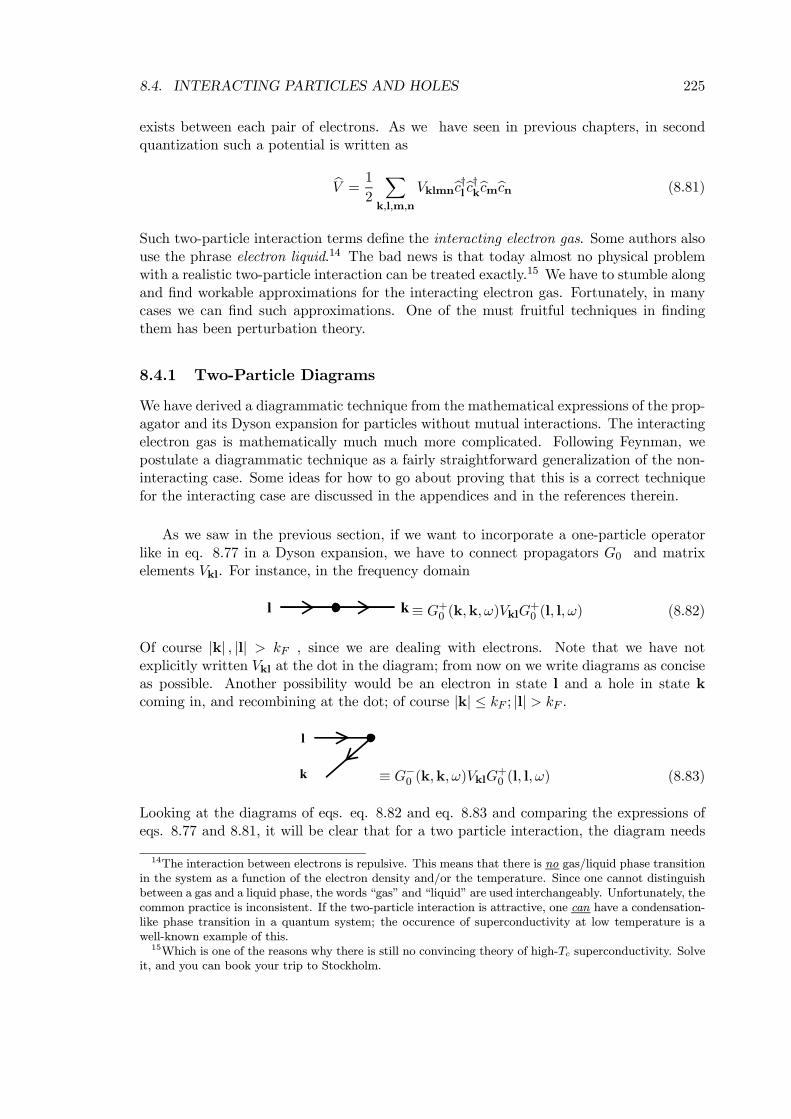
8.4. INTERACTING PARTICLES AND HOLES 225
exists between each pair of electrons. As we have seen in previous chapters, in secondquantization such a potential is written as
bV = 1
2
Xk,l,m,n
Vklmnbc†lbc†kbcmbcn (8.81)
Such two-particle interaction terms define the interacting electron gas. Some authors alsouse the phrase electron liquid.14 The bad news is that today almost no physical problemwith a realistic two-particle interaction can be treated exactly.15 We have to stumble alongand find workable approximations for the interacting electron gas. Fortunately, in manycases we can find such approximations. One of the must fruitful techniques in findingthem has been perturbation theory.
8.4.1 Two-Particle Diagrams
We have derived a diagrammatic technique from the mathematical expressions of the prop-agator and its Dyson expansion for particles without mutual interactions. The interactingelectron gas is mathematically much much more complicated. Following Feynman, wepostulate a diagrammatic technique as a fairly straightforward generalization of the non-interacting case. Some ideas for how to go about proving that this is a correct techniquefor the interacting case are discussed in the appendices and in the references therein.
As we saw in the previous section, if we want to incorporate a one-particle operatorlike in eq. 8.77 in a Dyson expansion, we have to connect propagators G0 and matrixelements Vkl. For instance, in the frequency domain
l k≡ G+0 (k,k,ω)VklG+0 (l, l,ω) (8.82)
Of course |k| , |l| > kF , since we are dealing with electrons. Note that we have notexplicitly written Vkl at the dot in the diagram; from now on we write diagrams as conciseas possible. Another possibility would be an electron in state l and a hole in state kcoming in, and recombining at the dot; of course |k| ≤ kF ; |l| > kF .
l
k ≡ G−0 (k,k,ω)VklG+0 (l, l,ω) (8.83)
Looking at the diagrams of eqs. eq. 8.82 and eq. 8.83 and comparing the expressions ofeqs. 8.77 and 8.81, it will be clear that for a two particle interaction, the diagram needs
14The interaction between electrons is repulsive. This means that there is no gas/liquid phase transitionin the system as a function of the electron density and/or the temperature. Since one cannot distinguishbetween a gas and a liquid phase, the words “gas” and “liquid” are used interchangeably. Unfortunately, thecommon practice is inconsistent. If the two-particle interaction is attractive, one can have a condensation-like phase transition in a quantum system; the occurence of superconductivity at low temperature is awell-known example of this.15Which is one of the reasons why there is still no convincing theory of high-Tc superconductivity. Solve
it, and you can book your trip to Stockholm.
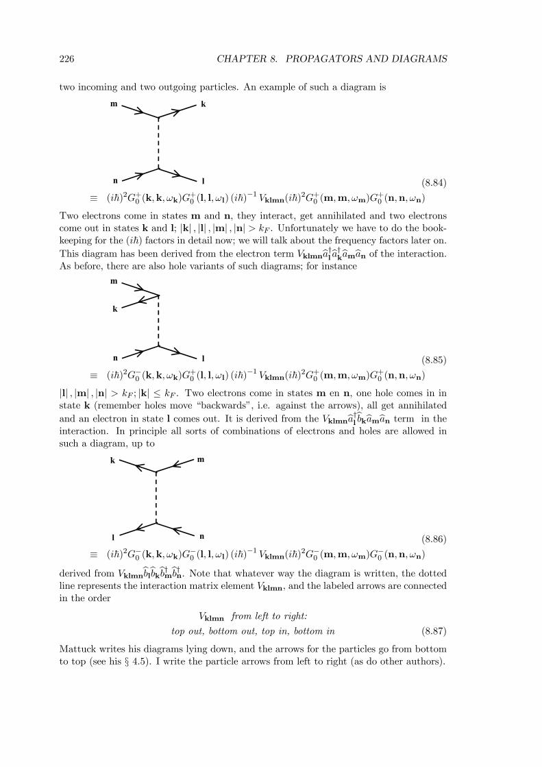
226 CHAPTER 8. PROPAGATORS AND DIAGRAMS
two incoming and two outgoing particles. An example of such a diagram is
l
km
n (8.84)
≡ (i~)2G+0 (k,k,ωk)G+0 (l, l,ωl) (i~)
−1 Vklmn(i~)2G+0 (m,m,ωm)G+0 (n,n,ωn)
Two electrons come in states m and n, they interact, get annihilated and two electronscome out in states k and l; |k| , |l| , |m| , |n| > kF . Unfortunately we have to do the book-keeping for the (i~) factors in detail now; we will talk about the frequency factors later on.This diagram has been derived from the electron term Vklmnba†lba†kbamban of the interaction.As before, there are also hole variants of such diagrams; for instance
l
k
m
n (8.85)
≡ (i~)2G−0 (k,k,ωk)G+0 (l, l,ωl) (i~)
−1 Vklmn(i~)2G+0 (m,m,ωm)G+0 (n,n,ωn)
|l| , |m| , |n| > kF ; |k| ≤ kF . Two electrons come in states m en n, one hole comes in instate k (remember holes move “backwards”, i.e. against the arrows), all get annihilated
and an electron in state l comes out. It is derived from the Vklmnba†lbbkbamban term in theinteraction. In principle all sorts of combinations of electrons and holes are allowed insuch a diagram, up to
l
k m
n (8.86)
≡ (i~)2G−0 (k,k,ωk)G−0 (l, l,ωl) (i~)
−1 Vklmn(i~)2G−0 (m,m,ωm)G−0 (n,n,ωn)
derived from Vklmnbblbbkbb†mbb†n. Note that whatever way the diagram is written, the dottedline represents the interaction matrix element Vklmn, and the labeled arrows are connectedin the order
Vklmn from left to right:
top out, bottom out, top in, bottom in (8.87)
Mattuck writes his diagrams lying down, and the arrows for the particles go from bottomto top (see his § 4.5). I write the particle arrows from left to right (as do other authors).
8.4. INTERACTING PARTICLES AND HOLES 227
8.4.2 The Homogeneous Electron Gas Revisited
For the interacting homogeneous electron gas there are no atomic potentials (eq. 8.75),but the electron-electron interaction (eq. 8.80) is present. The perturbation expansionand the associated diagrams become simpler. This is mainly because the two particlematrix elements Vklmn are simpler, since the single particle basis states are plane waves.
Vklmn =
Z Zd3r1 d
3r2 φ∗k(r1)φ
∗l (r2)
e2
|r1 − r2|φm(r1)φn(r2)
=e2
Ω2
Z Zd3r1 d
3r2 ei(m−k)·r1ei(n−l)·r2
1
|r1 − r2| (8.88)
(see Section 6.3.1, in particular eq. 6.41). The integral can be done by defining newintegration variables r = r1 − r2 and R =1
2(r1 + r2). The result is
Vklmn =1
Ωvk−m δk+l,m+n
where vq = e2Zd3r e−iq·r
1
r=4πe2
q2(8.89)
is the (three-dimensional) Fourier transform of the Coulomb potential e2
r . For a moredetailed derivation, see Mattuck p. 135.16 The δk+l,m+n can be interpreted like a “con-servation of momentum” selection rule. It can be incorporated in the diagrams. Definingq = k−m means we can write m = k− q and, because of the Kronecker δ, n = l+ q, sothe non-zero matrix elements are of the form
Vklmn = Vk,l,k−q,l+q =1
Ωvq (8.90)
We can relabel the generic diagram of eq. 8.84 as
l
kqkm −=
qln +=
q
(8.91)
Since in the homogeneous electron gas the one-particle states are plane waves, the labelsk, l etcetera correspond to the momenta of the particles. The diagram then tells us that thesum of the momenta of the incoming particlesm+ n is equal to the sum of the momenta ofthe outgoing particles k+ l. The diagram thus expresses the conservation of momentum.Adding the arrow labeled q explicitly gives the momentum which is transferred from thelower to the upper particle. The diagram can be interpreted in an intuitive way as a“collision” between two particles where momentum is transferred from one to the otherparticle. In the spirit of the previous chapter, one can apply “circuit” rules to this diagram.At each node the sum of the incoming arrows (read: momentum) has to be equal to the
16Note that, compared to Mattuck, I have surpressed the spin variables σ1 etcetera. In my case kimplicitly includes the spin variable. It becomes (k,σ1) in Mattuck’s notation.
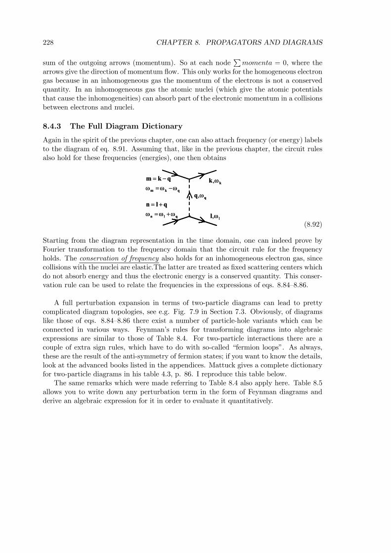
228 CHAPTER 8. PROPAGATORS AND DIAGRAMS
sum of the outgoing arrows (momentum). So at each nodePmomenta = 0, where the
arrows give the direction of momentum flow. This only works for the homogeneous electrongas because in an inhomogeneous gas the momentum of the electrons is not a conservedquantity. In an inhomogeneous gas the atomic nuclei (which give the atomic potentialsthat cause the inhomogeneities) can absorb part of the electronic momentum in a collisionsbetween electrons and nuclei.
8.4.3 The Full Diagram Dictionary
Again in the spirit of the previous chapter, one can also attach frequency (or energy) labelsto the diagram of eq. 8.91. Assuming that, like in the previous chapter, the circuit rulesalso hold for these frequencies (energies), one then obtains
,ωll
,ωkkω ω ω
= −= −m k q
m k q
ω ω ω= += +n l q
n l q,ωqq
,ωll
,ωkkω ω ω
= −= −m k q
m k q
ω ω ω= += +n l q
n l q,ωqq
(8.92)
Starting from the diagram representation in the time domain, one can indeed prove byFourier transformation to the frequency domain that the circuit rule for the frequencyholds. The conservation of frequency also holds for an inhomogeneous electron gas, sincecollisions with the nuclei are elastic.The latter are treated as fixed scattering centers whichdo not absorb energy and thus the electronic energy is a conserved quantity. This conser-vation rule can be used to relate the frequencies in the expressions of eqs. 8.84—8.86.
A full perturbation expansion in terms of two-particle diagrams can lead to prettycomplicated diagram topologies, see e.g. Fig. 7.9 in Section 7.3. Obviously, of diagramslike those of eqs. 8.84—8.86 there exist a number of particle-hole variants which can beconnected in various ways. Feynman’s rules for transforming diagrams into algebraicexpressions are similar to those of Table 8.4. For two-particle interactions there are acouple of extra sign rules, which have to do with so-called “fermion loops”. As always,these are the result of the anti-symmetry of fermion states; if you want to know the details,look at the advanced books listed in the appendices. Mattuck gives a complete dictionaryfor two-particle diagrams in his table 4.3, p. 86. I reproduce this table below.
The same remarks which were made referring to Table 8.4 also apply here. Table 8.5allows you to write down any perturbation term in the form of Feynman diagrams andderive an algebraic expression for it in order to evaluate it quantitatively.
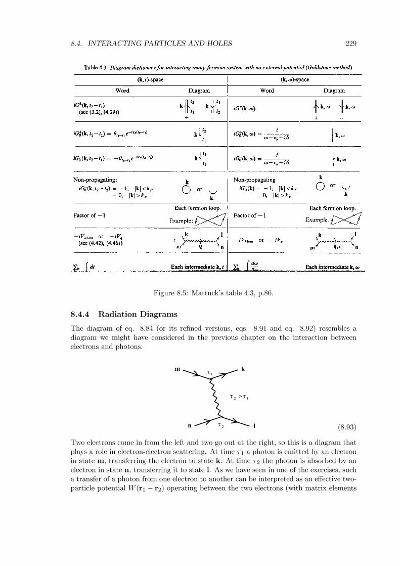
8.4. INTERACTING PARTICLES AND HOLES 229
Figure 8.5: Mattuck’s table 4.3, p.86.
8.4.4 Radiation Diagrams
The diagram of eq. 8.84 (or its refined versions, eqs. 8.91 and eq. 8.92) resembles adiagram we might have considered in the previous chapter on the interaction betweenelectrons and photons.
km
ln
1τ
2τ
12 ττ >
(8.93)
Two electrons come in from the left and two go out at the right, so this is a diagram thatplays a role in electron-electron scattering. At time τ1 a photon is emitted by an electronin state m, transferring the electron to state k. At time τ2 the photon is absorbed by anelectron in state n, transferring it to state l. As we have seen in one of the exercises, sucha transfer of a photon from one electron to another can be interpreted as an effective two-particle potential W (r1 − r2) operating between the two electrons (with matrix elements
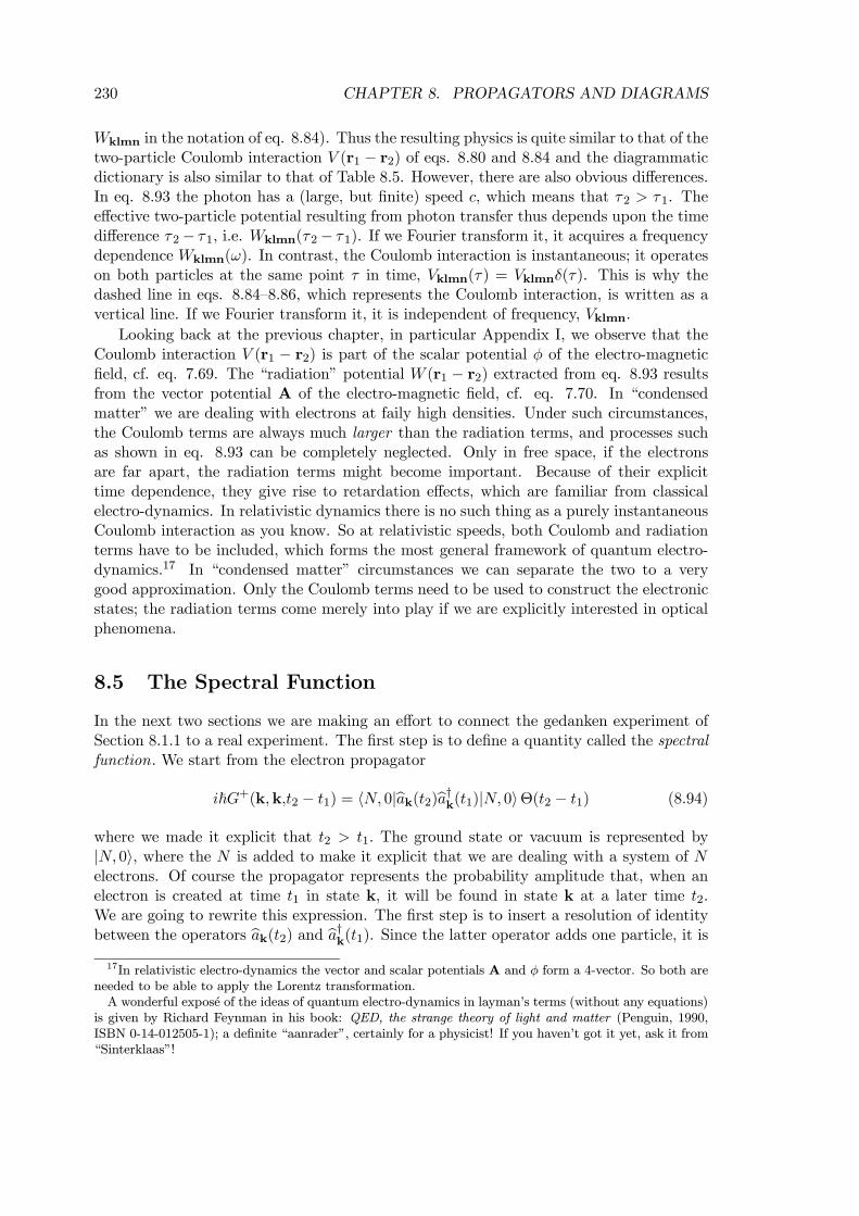
230 CHAPTER 8. PROPAGATORS AND DIAGRAMS
Wklmn in the notation of eq. 8.84). Thus the resulting physics is quite similar to that of thetwo-particle Coulomb interaction V (r1 − r2) of eqs. 8.80 and 8.84 and the diagrammaticdictionary is also similar to that of Table 8.5. However, there are also obvious differences.In eq. 8.93 the photon has a (large, but finite) speed c, which means that τ2 > τ1. Theeffective two-particle potential resulting from photon transfer thus depends upon the timedifference τ2− τ1, i.e. Wklmn(τ2− τ1). If we Fourier transform it, it acquires a frequencydependence Wklmn(ω). In contrast, the Coulomb interaction is instantaneous; it operateson both particles at the same point τ in time, Vklmn(τ) = Vklmnδ(τ). This is why thedashed line in eqs. 8.84—8.86, which represents the Coulomb interaction, is written as avertical line. If we Fourier transform it, it is independent of frequency, Vklmn.
Looking back at the previous chapter, in particular Appendix I, we observe that theCoulomb interaction V (r1 − r2) is part of the scalar potential φ of the electro-magneticfield, cf. eq. 7.69. The “radiation” potential W (r1 − r2) extracted from eq. 8.93 resultsfrom the vector potential A of the electro-magnetic field, cf. eq. 7.70. In “condensedmatter” we are dealing with electrons at faily high densities. Under such circumstances,the Coulomb terms are always much larger than the radiation terms, and processes suchas shown in eq. 8.93 can be completely neglected. Only in free space, if the electronsare far apart, the radiation terms might become important. Because of their explicittime dependence, they give rise to retardation effects, which are familiar from classicalelectro-dynamics. In relativistic dynamics there is no such thing as a purely instantaneousCoulomb interaction as you know. So at relativistic speeds, both Coulomb and radiationterms have to be included, which forms the most general framework of quantum electro-dynamics.17 In “condensed matter” circumstances we can separate the two to a verygood approximation. Only the Coulomb terms need to be used to construct the electronicstates; the radiation terms come merely into play if we are explicitly interested in opticalphenomena.
8.5 The Spectral Function
In the next two sections we are making an effort to connect the gedanken experiment ofSection 8.1.1 to a real experiment. The first step is to define a quantity called the spectralfunction. We start from the electron propagator
i~G+(k,k,t2 − t1) = hN, 0|bak(t2)ba†k(t1)|N, 0iΘ(t2 − t1) (8.94)
where we made it explicit that t2 > t1. The ground state or vacuum is represented by|N, 0i, where the N is added to make it explicit that we are dealing with a system of Nelectrons. Of course the propagator represents the probability amplitude that, when anelectron is created at time t1 in state k, it will be found in state k at a later time t2.We are going to rewrite this expression. The first step is to insert a resolution of identitybetween the operators bak(t2) and ba†k(t1). Since the latter operator adds one particle, it is17In relativistic electro-dynamics the vector and scalar potentials A and φ form a 4-vector. So both are
needed to be able to apply the Lorentz transformation.A wonderful expose of the ideas of quantum electro-dynamics in layman’s terms (without any equations)
is given by Richard Feynman in his book: QED, the strange theory of light and matter (Penguin, 1990,ISBN 0-14-012505-1); a definite “aanrader”, certainly for a physicist! If you haven’t got it yet, ask it from“Sinterklaas”!
8.5. THE SPECTRAL FUNCTION 231
clear that the resolution of identity must contain all the states of an N+1 particle system.Let’s simply number them |N + 1, ni;n = 0, 1, .... So
I =Xn
|N + 1, nihN + 1, n| (8.95)
All other |N 0,mihN 0,m| with N 0 6= N + 1 inserted in eq. 8.94 give zero contributionbecause they contain the wrong number of particles. At the same time we can insertbak(t) = bU †(t, 0)bak bU(t, 0) (which was its definition), and get
i~G+(k,k,t2 − t1) =Xn
hN, 0|bU †(t2, 0)bak bU(t2, 0)|N + 1, ni
hN + 1, n|bU †(t1, 0)ba†k bU(t1, 0)|N, 0iΘ(t2 − t1) (8.96)
We choose t1 = 0 and t2 = t to simplify our notation, write bU(t, 0) = e− i~ tbH for the time
evolution operator, and use
bH|N 0,mi = EN 0m |N 0,mi (8.97)
i.e. the states |N 0,mi are eigenstates of the full Hamiltonian; EN 0m is the energy of the
m’th state of an N 0 particle system. It is easy to see that eq. 8.96 now transforms into
i~G+(k,k,t) =Xn
e−i~ t(E
N+1n −EN0 )
¯³ba†k´n0
¯2Θ(t) where³ba†k´
n0= hN + 1, n|ba†k|N, 0i (8.98)
It is custom to rewrite
EN+1n −EN0 =³EN+1n −EN+10
´+³EN+10 −EN0
´(8.99)
because for a large system
EN+10 −EN0 ≡ µN+1 = µ (8.100)
becomes independent of N . The quantity µ is the (lowest possible) energy that is addedto a system when one particle is added. When the number of particles becomes very large(the so-called “thermodynamic limit”) µ becomes independent of the number of particles;in thermodynamics it is called the chemical potential.18 For metals at a temperatureT = 0 the chemical potential µ is identical to the Fermi energy ²F .
19 We also write
EN+1n −EN+10 ≡ ²N+1n0 (8.101)
These are the excitation energies of an N + 1 particle system. By the same reasoningas above, for a very large system the excitations of an N + 1 particle system will notbe different from those of an N particle system. The excitation energies will also be
18Consider a crystal, where the number of particles N > 1023, typically. Whether we add one extraelectron to 1023 electrons or to 1023 + 1 electrons will not make to much difference. This adds the sameamount of energy µ to the system.19In principle the formalism can be extended to a finite temperature, where the term chemical potential
is perhaps more familiar.
232 CHAPTER 8. PROPAGATORS AND DIAGRAMS
independent of the number of particles in the thermodynamic limit. Using eqs. 8.100 and8.101 in eq. 8.98 yields
i~G+(k,k,t) =Xn
e−i~ t(²
N+1n0 +µ)
¯³ba†k´n0
¯2Θ(t) (8.102)
The spectral function is defined by
A+(k,ω) =Xn
¯³ba†k´n0
¯2δ(~ω−²N+1n0 ) (8.103)
It is also called the spectral density or the spectral density function. Obviously the spectralfunction is positive definite, i.e. A+(k,ω) ≥ 0. We can rewrite eq. 8.102 as
i~G+(k,k,t) =Z ∞
−∞dω e−
i~ t(ω+µ)A+(k,ω)Θ(t) (8.104)
A similar rewriting can be done for the hole propagator
−i~G−(k,k,t) = hN, 0|bbk(0)bb†k(t)|N, 0iΘ(−t)=
Z ∞
−∞dω e
i~ t(ω−µ)A−(k,ω)Θ(−t) (8.105)
with a spectral density for holes defined as
A−(k,ω) =Xn
¯³bb†k´n0
¯2δ(~ω−²N−1n0 ) (8.106)
where we have used EN0 − EN−10 ≡ µN = µ analogous to eq. 8.101 and ²N−1n0 = EN−1n −EN−10 are the excitation energies of the N−1 particle system. “−” signs have been placedat the relevant places in order to keep everything consistent for holes. Obviously alsoA−(k,ω) ≥ 0. The spectral function can be used to investigate the analytical mathematicalproperties of propagators. That however is best left to the mathematicians; we are moreconcerned with its physical role.
8.5.1 Physical Content
The spectral function plays an important physical role because it is connected to lineshapes in spectra (see also the next section). In order to reproduce the particle and holepropagators of free, unperturbed particles of eqs. 8.14 and eq. 8.27 one has to use
A±0 (k,ω) =δ(~ω ∓ (²k − µ)) (8.107)
in eqs. 8.104 and 8.105. The spectral function thus gives a δ-peak at an energy relativeto the Fermi level, i.e. at ²k − µ for ²k > µ (particles) and at µ − ²k for ²k < µ (holes).In order to reproduce the quasi-particle (or -hole) forms of the propagators, cf. eqs. 8.17,8.32 and 8.73, the spectral functions to be used in eqs. 8.104 and 8.105 are
A±(k,ω) =zkπ
Γk/2
[~ω ∓ (²k +∆k − µ)]2 + (Γk/2)2(8.108)
So compared to the free particles (holes), the spectral functions for quasi-particles (-holes)are transformed from δ-peaks into Lorentzian line shapes; see e.g. Fig. 4.14. The peakmaximum is given by ²k+∆k−µ, for ²k+∆k > µ (particles) and µ−²k−∆k for ²k+∆k < µ(holes), hence the name “level shift” for ∆k, if one compares to the unperturbed case. Inboth cases the width of the peak is determined by Γk.
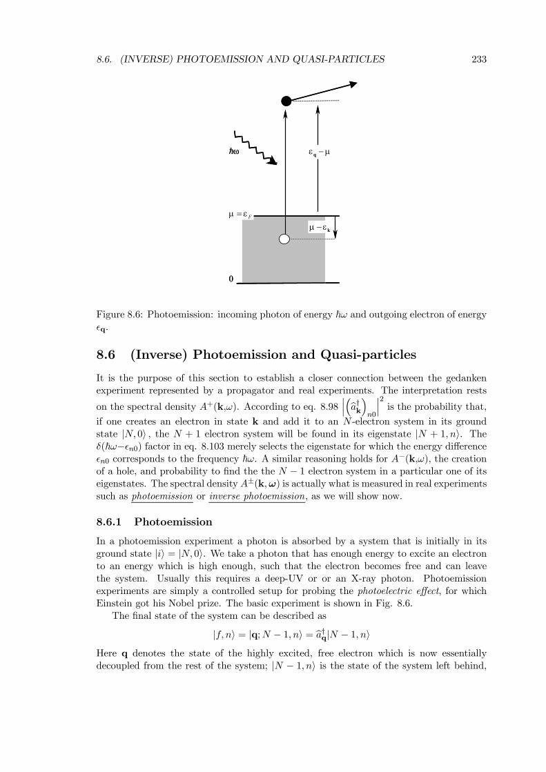
8.6. (INVERSE) PHOTOEMISSION AND QUASI-PARTICLES 233
Fµ ε=
0
µ ε− k
ε µ−qω
Fµ ε=
0
µ ε− k
ε µ−qω
Figure 8.6: Photoemission: incoming photon of energy ~ω and outgoing electron of energy²q.
8.6 (Inverse) Photoemission and Quasi-particles
It is the purpose of this section to establish a closer connection between the gedankenexperiment represented by a propagator and real experiments. The interpretation rests
on the spectral density A+(k,ω). According to eq. 8.98¯³ba†k´
n0
¯2is the probability that,
if one creates an electron in state k and add it to an N -electron system in its groundstate |N, 0i , the N + 1 electron system will be found in its eigenstate |N + 1, ni. Theδ(~ω−²n0) factor in eq. 8.103 merely selects the eigenstate for which the energy difference²n0 corresponds to the frequency ~ω. A similar reasoning holds for A−(k,ω), the creationof a hole, and probability to find the the N − 1 electron system in a particular one of itseigenstates. The spectral densityA±(k,ω) is actually what is measured in real experimentssuch as photoemission or inverse photoemission, as we will show now.
8.6.1 Photoemission
In a photoemission experiment a photon is absorbed by a system that is initially in itsground state |ii = |N, 0i. We take a photon that has enough energy to excite an electronto an energy which is high enough, such that the electron becomes free and can leavethe system. Usually this requires a deep-UV or or an X-ray photon. Photoemissionexperiments are simply a controlled setup for probing the photoelectric effect, for whichEinstein got his Nobel prize. The basic experiment is shown in Fig. 8.6.
The final state of the system can be described as
|f, ni = |q;N − 1, ni = ba†q|N − 1, niHere q denotes the state of the highly excited, free electron which is now essentiallydecoupled from the rest of the system; |N − 1, ni is the state of the system left behind,
234 CHAPTER 8. PROPAGATORS AND DIAGRAMS
which has one hole in it. We keep the label n to distinguish between the possible finalstates. The outgoing electron is detected and its energy ²q is measured by the detector.
20
Its momentum ~q can be obtained by measuring the direction of the outgoing electronand using ~q =
p2m²q for its size. The state q of the outgoing free electron can thus
be characterized completely. Obviously the state of the incoming photon is completelycharacterized by its energy ~ω and its momentum ~K. We assume that Fermi’s goldenrule holds for the absorption process, which means that the light source must not betoo strong in order for first order perturbation theory to hold. The transition rate forphotoemission wPE then becomes
wPE ∝Xn
¯hf, n|bV |ii¯2 δ ¡~ω−[²q +EN−1n −EN0 ]
¢=
Xn
¯hN − 1, n|baqbV |N, 0i¯2 δ ¡~ω−[²q +EN−1n −EN0 ]
¢(8.109)
The δ-function says that the photon energy ~ω must make up for the difference betweenthe initial state energy EN0 , and the final state energy, which is the sum of the energy ²qof the free electron and the energy EN−1n of the system left behind. The perturbationoperator bV describes the absorption process; it has been discussed in Section 7.2, eqs.7.35—7.38 Since we are not interested in photons right now, we will focus solely on itselectronic part. Since an electron has to be excited from below the Fermi level to abovethe Fermi level, the term that contributes must have the form
bV = X|l|>kF ,|k|≤kF
Vlkba†lbb†k (8.110)
The individual terms in the sum create a hole below the Fermi level and an electron aboveit.21 Using eq. 8.110 in eq. 8.109 gives products like baqba†kbb†l . Using the anti-commutationrelations for Fermion operators we can rewrite them as
baqba†kbb†k = δqlbb†k − ba†lbaqbb†k= δqlbb†k + ba†lbb†kbaq (8.111)
If we apply this expression in eq. 8.109, the second term of it contributes zero because
baq|N, 0i ≈ 0 (8.112)
i.e. a “free” electron in a high energy state has negligible overlap with the system’s groundstate. This is a crucial point. For a system of non-interacting electrons eq. 8.112 is exact,since the high-energy state |qi is not occupied in the ground state and so there is nothing toannihilate by baq. For a system of interacting electrons, eq. 8.112 is only an approximation.20This is not the full story, since an electron that crosses the surface of a material has to increase its
(electrostatic) potential (if the potential inside a material would not be lower than in vacuum, then allthe electrons would fly off spontaneously). The energy of the detected electron is ²q − V0, where V0 is theelectrostatic potential level in vacuum, far from the material. In order not too complicate the notation,we have omitted V0 here. It will merely shift the photoemission spectrum by a constant.21Other possible terms in this operator are
P|l|>kF ,|k|>kF Vlkba†lbak; P
|l|≤kF ,|k|>kF Vlkbblbak andP
|l|≤kF ,|k|≤kF Vlkbblbb†k. These terms however do not participate in the absorption as can easily be shown
(the second term gives emission, for instance).
8.6. (INVERSE) PHOTOEMISSION AND QUASI-PARTICLES 235
However, the approximation becomes better the higher the energy of the “free” electron.In the practice of photoemission it works very well. Only the first term in eq. 8.111 isthus retained and eq. 8.109 becomes
wPE ∝X
n,|k|≤kF
¯hN − 1, n|bb†k|N, 0i¯2 |Vqk|2 δ ³~ω−[²q + ²N−1n0 − µ]
´=
X|k|≤kF
A−(k, [²− ²q+µ]/~) |Vqk|2 = V 2PEX|k|≤kF
A−(k, [²− ²q + µ]/~)(8.113)
where we have written ² = ~ω for the energy of the incoming photon and used the definitionof the spectral function, eq. 8.106. If the transition matrix element Vqk is not verydependent on the states, as is often the case when the energy ²q of the “free” electron ishigh enough, we can approximate it by a single number VPE. This is the second crucialpoint. We can write
wPE ∝= V 2PEX|k|≤kF
A−(k, [²− ²q + µ]/~) (8.114)
Then the photoemission transition rate wPE is directly proportional to the spectral densityA−. The photoemission signal is proportional to the transition rate, so the spectral densityof a material is directly measured in a photoemission experiment !
8.6.2 Inverse Photoemission
Inverse photoemission is the following experiment. One comes in with an electron at arelatively high energy ² = ~ω. This electron is captured by the material and transferredto a lower energy level (decited ?), where at the same time a photon of energy ~ωq = ²q isemitted. The photon is detected and its energy and momentum are measured. The basicidea is shown in Fig. 8.7.
The experiment is the inverse of photoemission; hence its name. It is also known underthe name “Bremsstrahlung isochromat spectroscopy” (BIS), i.e. spectrally resolved lightproduced by slowing down an electron. It is easy to prove under the same conditions asabove that the transition rate for inverse photoemission wIPE(ω), and thus the inversephotoemission signal, is proportional to the spectral density A+.
wIPE ∝ V 2IPEX|k|>kF
A+(k, [²− ²q − µ]/~) (8.115)
EXAMPLES
It is instructive to consider some examples. First inverse photoemission from a systemwhich consists of non-interacting particles. The spectral function then has the form givenby eq. 8.107 and inserted in eq. 8.115 one gets
wIPE ∝ V 2IPEX|k|>kF
δ(²− ²q − ²k) (8.116)
A δ-peak appears in the spectrum whenever the energy of the incoming electron minusthat of the outgoing photon, ² − ²q, coincides with an energy-level ²k which is available
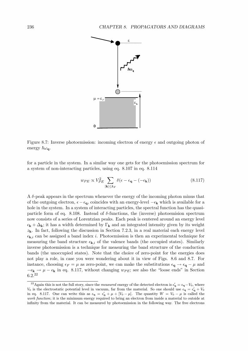
236 CHAPTER 8. PROPAGATORS AND DIAGRAMS
0
εk
ωq
Fµ ε=
ε
0
εk
ωq
Fµ ε=
ε
Figure 8.7: Inverse photoemission: incoming electron of energy ² and outgoing photon ofenergy ~ωq.
for a particle in the system. In a similar way one gets for the photoemission spectrum fora system of non-interacting particles, using eq. 8.107 in eq. 8.114
wPE ∝ V 2PEX|k|≤kF
δ(²− ²q − (−²k)) (8.117)
A δ-peak appears in the spectrum whenever the energy of the incoming photon minus thatof the outgoing electron, ²− ²q, coincides with an energy-level −²k which is available for ahole in the system. In a system of interacting particles, the spectral function has the quasi-particle form of eq. 8.108. Instead of δ-functions, the (inverse) photoemision spectrumnow consists of a series of Lorentzian peaks. Each peak is centered around an energy level²k +∆k; it has a width determined by Γk and an integrated intensity given by its weightzk. In fact, following the discussion in Section 7.2.3, in a real material each energy level²k,i can be assigned a band index i. Photoemission is then an experimental technique formeasuring the band structure ²k,i of the valence bands (the occupied states). Similarlyinverse photoemission is a technique for measuring the band structure of the conductionbands (the unoccupied states). Note that the choice of zero-point for the energies doesnot play a role, in case you were wondering about it in view of Figs. 8.6 and 8.7. Forinstance, choosing ²F = µ as zero-point, we can make the substitutions ²q → ²q − µ and−²k → µ − ²k in eq. 8.117, without changing wPE; see also the “loose ends” in Section6.2.22
22Again this is not the full story, since the measured energy of the detected electron is ²0q = ²q−V0, whereV0 is the electrostatic potential level in vacuum, far from the material. So one should use ²q = ²0q + V0in eq. 8.117. One can write this as ²q = ²0q + µ + [V0 − µ]. The quantity W = V0 − µ is called thework function; it is the minimum energy required to bring an electron from inside a material to outside atinfinity from the material. It can be measured by photoemission in the following way. The free electrons
8.7. APPENDIX I. THE ADIABATIC CONNECTION 237
8.7 Appendix I. The Adiabatic Connection
8.7.1 The Problem
Consider again the electron propagator
i~G+(k,m, t2 − t1) =DΨ0
¯bak (t2)ba†m (t1)¯Ψ0E (8.118)
For a system of particles that interact with one another, or with atomic potentials, ob-viously |Ψ0i is the ground state or vacuum of the full system, i.e. including all interac-tions. We argued that one has to make a perturbation expansion of the time evolutionoperator when working out the operators bak (t2) = bU †(t2, 0)bak bU(t2, 0) and ba†m (t1) =bU †(t1, 0)ba†m bU(t1, 0). This should be equivalent to a diagram expansion as discussed. How-ever, translating diagrams into algebra again using Table 8.4, one obtains expressions thatcontain unperturbed G0(m,k, t2 − t1)’s and simple matrix elements only. It is not at allobvious that this is correct. There are two problems.
1. The trick we used in Section 8.2.2, which is inserting resolutions of identity betweeneach pair of operators, cf. eq. 8.23, is no good in general. We get matrix elementslike hΨ0 |bak|ni, with |ni some n-particle/hole state. The state |Ψ0i is an eigenstateof the full Hamiltonian (the ground state), which includes the perturbation, so thereis no simple expression for this matrix element. Whereas in the example treated inSection 8.3.1 |Ψ0i could be obtained in principle, albeit after some calculation, thisis not so for the interacting electron gas. The ground state of an interacting electronsystem can in general not be obtained exactly.23 It does not make much sense thento even write down a matrix element like hΨ0 |bak|ni, since we can not evaluate it.
2. To add to our problems, we used |k| ≤ kF and |k| > kF to distinguish betweenelectron and hole states. This distinction was based upon the non-interacting elec-tron gas, where we could fill up the one electron states one by one, starting at thebottom up to the Fermi level, see Section 6.3.1. In stone-age notation the states ofthe non-interacting electron gas can be expressed as
|k1k2....kNi(a) = |k1ik2i....|kN i(a) (8.119)
where in the ground state |k1| ≤ |k2| ≤ .... ≤ |kN | = kF . This is not an eigenstateof a full Hamiltonian, when we include atomic potential and/or electron-electroninteractions. If we use states like those of eq. 8.119 as a basis set, the ground stateof the full Hamiltonian is a linear combination of such states, in which also stateswith |k| > kF are involved, see e.g. eq. 8.37 in Section 8.3. On forehand it is notclear what role the Fermi energy or wave number kF plays in an interacting system;indeed it is not clear that it plays any role at all. In any case, kF will not be “sharp”in an interacting system, in the sense that the probability of observing an electron
of highest energy are produced from the Fermi level, i.e. using ²k = ²F = µ in eq. 8.117, see also Fig. ??.Using these expressions ²k and ²q in eq. 8.117 gives a δ(²− ²0q−W ) corresponding to the freed electrons ofhighest energy. Since ² and ²0q are measured, the work function W can be obtained. See also A. Zangwill,Physics at Surfaces, (Cambridge Un. Press, Cambridge, 1988).23For a homogeneous interacting electron gas the ground state wave function can be obtained only
after a very lengthy computation using the so-called Quantum Monte Carlo approach. Calculations forinhomogeneous systems (i.e. which include atomic potentials) are a topic of present research.
238 CHAPTER 8. PROPAGATORS AND DIAGRAMS
in a state with |k| ≤ kF is one and in a state with |k| > kF it is zero. At best thisprobability will change with increasing |k| from close to one to close to zero near acharacteristic wave number kF . At worst, the probability will change smoothly andno clear kF can be distinguished.
24
So have we been staging a hoax in assuming that one may use the diagrams of Table8.4? Well, we have not, but the solution to the problems discussed above involves someintricate reasoning. It can be found in Mattuck, Appendices B—G. I will walk you throughthe reasoning up to and including Appendix E. The ultimate solution lies in the famous“Wick’s theorem”, which is discussed in Appendix F, and the proof that the diagram-matic procedure followed in Section 8.3 is correct is found in Appendix G. The followingAppendix II gives a simplified (but non-general) discussion of this case.
8.7.2 The Solution
To facilitate formal operations, the propagator is written as
i~G(k,m, t2 − t1) =DΨ0
¯Tnbak (t2)ba†m (t1)o¯Ψ0E (8.120)
where T ... is Wick’s time ordering operator, cf. eqs. 8.10 and 8.11. It leads to
i~G(k,m, t2 − t1) = i~G+(k,m, t2 − t1) t2 > t1
= i~G−(k,m, t2 − t1) t2 ≤ t1 (8.121)
The main idea behind the time ordering operator is that it allows for a compact expressionof the electron propagator G+ and the hole propagator G− into one propagator G. Thegeneral definition of Wick’s time ordering operator is T
n bA(ta) bB(tb)... bZ(tz)o = (−1)p×the operators bA(ta), bB(tb), ..., bZ(tz) rearranged such, that times ..ti, tj , ... increase fromright to left. In case two times are equal, an annihilation operator comes to the right ofa creation operator of the same time. p is the number of interchanges needed to get allthe operators in the right order and it accounts for the anti-commutation rules of Fermionoperators.
We have a look at the time-dependent perturbation expansion again. Mattuck explainsit in his Appendix B and D; it should look very familiar to you, as we discussed it in thefirst chapters. He uses a slightly different notation, which is explained in the followingtable
My notation Mattuck’s notation WherebV H1 perturbationbUI(t, t0) = bU †0(t, 0)bU(t, t0) eU(t, t0) eq. D.1, p.356bVI(t) = bU †0(t, 0)bV bU0(t, 0) eH1 eq. D.5baI,k(t) = bU †0(t, 0)bak bU0(t, 0) bak(t) eq. D.5
24For “normal” electron systems, which are called Fermi liquids, the situation is actually “at best” anda clear Fermi wave number can still be distinguished. A discussion of this is presented in Mattuck’s §11.3,p.209; note especially the figures 11.1-11.3.
8.7. APPENDIX I. THE ADIABATIC CONNECTION 239
Using this table as a tool for translation, you should be able to recognize eq. D.10,Mattuck p.357 from my lecture notes. The first useful theorem is due to Dyson. It links theterms of the time-dependent perturbation expansion, which I have introduced in Chapter2, eq. 2.20, to an expression involving the time ordering operator we have just discussed
bU (n)I (t, t0) =
µ1
i~
¶n Z t
t0
dτn
Z τn
t0
dτn−1Z τn−1
t0
dτn−2......Z τ3
t0
dτ2
Z τ2
t0
dτ1
bVI (τn) bVI (τn−1) bVI (τn−2) ......bVI (τ2) bVI (τ1)=
1
n!
µ1
i~
¶n Z t
t0
dτn
Z t
t0
dτn−1Z t
t0
dτn−2......Z t
t0
dτ2
Z t
t0
dτ1
TnbVI (τn) bVI (τn−1) bVI (τn−2) ......bVI (τ2) bVI (τ1)o (8.122)
All the time integrals now run from t0 to t, which is convenient. This theorem can beproved using induction.
Now we address our main problem. We do know the ground state of the non-interacting(i.e. the unperturbed) system bH0|Φ0i = E0,0|Φ0i, but we don’t know the ground state
of the interacting (i.e. the perturbed) system ( bH0 + bV )|Ψ0i = E0|Ψ0i. We apply theadiabatic theorem. Suppose at t = −∞ our system is in the unperturbed ground state|Φ0i. Then we turn on the perturbation bV “adiabatically slow” by bV e−α|t|, with α avery small, real and positive number. The adiabatic theorem then states that at t = 0,the system is in the ground state of the perturbed Hamiltonian
|Ψ0i = N− 12 limα→0+
bUI(0,−∞)|Φ0i (8.123)
The proof of the adiabatic theorem is found by a straightforward generalization of one ofthe exercises. N is a normalization factor we will derive below. Now we switch off theperturbation again, again infinitely slow by bV e−α|t|. By applying the adiabatic theoremagain, we find that at t = ∞ the system is back in the ground state of the unperturbedHamiltonian
|Φ0i = N12 limα→0+
bUI(∞, 0)|Ψ0i⇔|Ψ0i = N−
12 limα→0+
bUI(0,∞)|Φ0i (8.124)
where the last line follows from the properties of the time-evolution operator bU−1I (t1, t2) =bUI(t2, t1). The normalization factor N is obtained from
NhΨ0|Ψ0i = N = hΦ0|bU †I (0,∞)bUI(0,−∞)|Φ0i= hΦ0|bUI(∞, 0)bUI(0,−∞)|Φ0i = hΦ0|bUI(∞,−∞)|Φ0i (8.125)
The basic idea is that we can derive the ground state of the perturbed system from thatof the unperturbed system by this adiabatic switching and, via eq. 8.122, we can make aperturbation expansion of the time-evolution operator bUI(t2, t1). This we can put to usein our propagator of eq. 8.120.
240 CHAPTER 8. PROPAGATORS AND DIAGRAMS
It remains to rewrite the propagator a bit. Write
bak(t) = bU †(t, 0)bak bU(t, 0)= bU †(t, 0)bU0(t, 0)bU †0(t, 0)bak bU0(t, 0)bU †0(t, 0)bU(t, 0)= bU †I (t, 0)baI,k(t)bUI(t, 0) (8.126)
using the definitions of the table above. Using eqs. 8.123—8.126 in eq. 8.120 then gives
i~G(k,m, t2 − t1) =hΦ0|bUI(∞, t2)baI,k(t2)bUI(t2, t1)ba†I,m(t1)bUI(t1,−∞)|Φ0i
hΦ0|bUI(∞,−∞)|Φ0iwhere properties of the time evolution operator like bUI(t1, 0)bUI(0,−∞) = bUI(t1,−∞) andbU †I (t1, t2) = bUI(t2, t1) have been applied. With the time-ordering operator we can give amore compact expressionbUI(∞, t2)baI,k(t2)bUI(t2, t1)ba†I,m(t1)bUI(t1,−∞) =
TnbUI(∞, t2)baI,k(t2)bUI(t2, t1)ba†I,m(t1)bUI(t1,−∞)o =
TnbUI(∞,−∞)baI,k(t2)ba†I,m(t1)o
In conclusion, the propagator is given by the expression
i~G(k,m, t2 − t1) =hΦ0|T
nbUI(∞,−∞)baI,k(t2)ba†I,m(t1)o |Φ0ihΦ0|bUI(∞,−∞)|Φ0i (8.127)
We now have what we wanted; all the matrix element are between |Φ0i, the ground stateof the non-interacting (the unperturbed) system. We know how to handle this. All theproblems we complained about at the beginning of this appendix vanish because we canwork with |Φ0i, which has the form given in eq. 8.119. The prize that we are paying isthat the expression of eq. 8.127 is much more complex than that of eq. 8.120, due tothe bUI terms. We can make a series expansion of this operator, the n’th term of which isgiven by eq. 8.122. The result is
i~G(k,m, t2 − t1) =∞Xn=0
1
n!
µ1
i~
¶n Z ∞
−∞dτn......
Z ∞
−∞dτ2
Z ∞
−∞dτ1
hΦ0|TnbVI (τn) ......bVI (τ2) bVI (τ1)baI,k(t2)ba†I,m(t1)o |Φ0i
∞Xn=0
1
n!
µ1
i~
¶n Z ∞
−∞dτn......
Z ∞
−∞dτ2
Z ∞
−∞dτ1
hΦ0|TnbVI (τn) ......bVI (τ2) bVI (τ1)o |Φ0i (8.128)
The expressions for the operators bVI and baI,k can be found from the table.25 In the inter-
acting many-particle system the perturbation bV is formed by two-particle interactions,
25Note we have to use adiabatic switching on and off so we have to modify bV by the time factor e−α|t|.An elegant alternative for this is not to modify bV and, instead of integrating over real times τ i; i = 1, .., n,to integrate slightly below the real axis from τ i = −∞(1− iα) to ∞(1− iα); this then automatically addsthe time factors e−α|t|.
8.8. APPENDIX II. THE LINKED CLUSTER EXPANSION 241
which according to Chapter 6, eq. 6.35 can be written as
bV =1
2
Xklmn
Vklmnba†lba†kbamban from which it is easy to prove
bVI(t) =1
2
Xklmn
Vklmnba†I,l(t)ba†I,k(t)baI,m(t)baI,n(t) (8.129)
Perturbing atomic potentials of course have a one-particle form, according to eq. 6.34 inChapter 6
bV =Xkl
Vklba†kbal from which one gets
bVI(t) =Xkl
Vklba†I,k(t)baI,l(t) (8.130)
Using either of the expressions of eqs. 8.129 or 8.130 in eq. 8.128 one observes that thecalculation amounts to computing a large number of matrix elements of the type
hΦ0|Tnba†I,l (τn) ......baI,n (τ1)baI,k(t2)ba†I,m(t1)o |Φ0i
Rather than doing all the algebra by hand, this can be done in an elegant way usingWick’stheorem, as explained in Mattuck’s Appendix F. From it follows the diagram expansionas we have used it in this chapter, using another elegant theorem called the linked clustertheorem, cf. Mattuck’s Appendix G.
The whole process relies upon the “adiabatic switching on/off” trick by which we“construct” the ground state |Ψ0i of our interacting system of particles from the groundstate |Φ0i of the system of non-interacting particles. This trick usually works fine, butit is not garanteed to work. If you look back the relevant exercize (or read Mattuck’sAppendix D), the trick fails if
hΦ0|Ψ0i = 0
i.e. when there is no overlap between the ground state of the non-interacting systemand the ground state of the interacting system. This is not usually the case, but it doeshappen occasionally. Superconductors are an example where the adiabatic trick fails; seeMattuck’s Chapter 15. This however is another story, and I am not the man to tell it.
8.8 Appendix II. The Linked Cluster Expansion
In this appendix we will try to evaluate the expression of eq. 8.39 of Section 8.3 step bystep using straight-forward algebra. It reads
i~G+(A,A, t2 − t1) =h00|bUI(∞, t2)baI,A(t2)bUI(t2, t1)ba†I,A(t1)bUI(t1,−∞)|00i
h00|bUI(∞,−∞)|00i (8.131)
The end result will be something called the linked cluster expansion. I will not try to proveit fully, since that would be too involved even for this rather simple model, but only make
242 CHAPTER 8. PROPAGATORS AND DIAGRAMS
it plausible to you. A full derivation based uponWick’s theorem can be found in Mattuck’sappendices F and G for the (non-interacting) many particle case. Proofs for interactingmany particle cases can be found in advanced books on many particle physics.26
8.8.1 Denominator
We first do the denominator h00|bUI(∞,−∞)|00i of eq. 8.131. We use the expansion ofeqs. 2.19 and 2.20 in Chapter 2 and get up to second order
h00|bUI(t, t0)|00i = h00|I + 1
i~
Z t
t0
dτ1 bVI (τ1)+
µ1
i~
¶2 Z t
t0
dτ2
Z τ2
t0
dτ1 bVI (τ2) bVI (τ1) |00i (8.132)
where
bVI (τ) = bU †0 (τ , t0) hbV e−α|τ |i bU0 (τ , t0) (8.133)
and
bV = X|k|>kF
³VkAba†kbaA + VAkba†Abak´+ X
|k|≤kF
³VkAbbkbaA + VAkba†Abb†k´ (8.134)
as in eq. 8.45. I prefer to let the time limits t0, t stand for a while and take the limit to−∞,∞ later on. Note that the exponential factors e−α|τ | ensure that the integrals alwaysconverge. The zero’th order term in eq. 8.132 is trivial. It gives h00|I|00i = h00|00i = 1;the state is normalized. The unperturbed time-evolution operator simply gives
bU0 (τ , t0) |00i = e− i~ (τ−t0) bH0 |00i = e− i
~ (τ−t0)E0 |00i (8.135)
since according to eqs. 8.33 and 8.41
bH0 = E0 − X|k|≤kF
²kbb†kbbk + X|k|>kF
²kba†kbak + ²Aba†AbaA (8.136)
The first order term of eq. 8.132 becomes
bU (1)I (t, t0) =1
i~
Z t
t0
dτ1 e−α|τ1|h00|bU †0 (τ1, t0) bV bU0 (τ1, t0) |00i = 1
i~
Z t
t0
dτ1 e−α|τ1|h00|bV |00i
=1
i~
Z t
t0
dτ1 e−α|τ1| X
|k|≤kFVAkh00|ba†Abb†k|00i = 0 (8.137)
because h00|ba†Abb†k|00i = h00|1A1ki = 0; the states of the number representation form an
orthonormal basis set. Note that the time factors resulting from bU0 and bU †0 cancel. Note26Such as, A. L. Fetter and J. D. Walecka, Quantum Theory of Many-Particle Systems, (McGraw-Hill,
Boston, 1971); S. Doniach And E. H. Sondheimer, Green’s Functions for Solid State Physicists, (ImperialCollege Press, London, 1998); G. D. Mahan, Many Particle Physics, (Plenum, New York, 2000). J. W.Negele and H. Orland, Quantum Many-Particle Systems, (Addison-Wesley, Redwood City, 1988).
8.8. APPENDIX II. THE LINKED CLUSTER EXPANSION 243
also that the other three terms in the perturbation bV give zero since they try to annihilatea a particle in the ground state (which does not contain any particles).
The second order term can be written as
bU (2)I (t, t0) =
µ1
i~
¶2 Z t
t0
dτ2 e−α|τ2|
Z τ2
t0
dτ1 e−α|τ1| h00|bU †0(τ2, t0)bV bU0 (τ2, τ1) bV bU0 (τ1, t0) |00i
=
µ1
i~
¶2 Z t
t0
dτ2 e−α|τ2|
Z τ2
t0
dτ1 e−α|τ1|
ei~ (τ2−t0)E0h00|bV bU0 (τ2, τ1) bV |00ie− i
~ (τ1−t0)E0 (8.138)
Using bV |00i =P|k|≤kF VAkba†Abb†k|00i =P|k|≤kF VAk|1A1ki we rewrite this as
bU (2)I (t, t0) =
µ1
i~
¶2 Z t
t0
dτ2 e−α|τ2|
Z τ2
t0
dτ1 e−α|τ1|
ei~ (τ2−τ1)E0
X|k|,|l|≤kF
V ∗AkVAlh1A1k|e−i~ (τ2−τ1) bH0 |1A1li
=
µ1
i~
¶2 Z t
t0
dτ2 e−α|τ2|
Z τ2
t0
dτ1 e−α|τ1|X
|k|≤kFe−
i~ (τ2−τ1)²Ae
i~ (τ2−τ1)²k |VAk|2 (8.139)
since
e−i~ (τ2−τ1) bH0 |1A1li = e− i
~ (τ2−τ1)(E0+²A−²l)|1A1li for |l| ≤kF (8.140)
and h1A1k|1A1li = δk,l. This is easily obtained from eq. 8.136 by noting that bH0 onlycontains number operators, i.e. bnh,l = bb†lbbl; bne,l = ba†lbal count the number of holes orelectrons in state l, respectively, and bnA = ba†AbaA counts the number of electrons in theatomic state A. Obviously the state |1A1li with |l| ≤kF has one hole in state l and oneelectron in the atomic state A.
The final result of eq. 8.139 can be given a nice diagrammatic interpretation in termsof “unperturbed” propagators. The unperturbed electron propagator is defined as
i~G+0 (l,k, t2 − t1) =D00
¯baI,l (t2)ba†I,k (t1)¯ 00E ; t2 > t1; |k|, |l| >kF=D00
¯ bU †0 (t2, 0)bal bU0 (t2, t1)ba†k bU0 (t1, 0)¯ 00E = e i~ (t2−t1)E0 D00 ¯bal bU0 (t2, t1)ba†k ¯ 00E= e
i~ (t2−t1)E0
D1l
¯ bU0 (t2, t1)¯ 1kE (8.141)
which is similar to the full propagator of eq. 8.46, but with unperturbed states andevolution operators. It follows
i~G+0 (l,k, t2 − t1) = ei~ (t2−t1)E0e−
i~ (t2−t1)(E0+²k)h1l|1ki
= e−i~ (t2−t1)²kδl,k; t2 > t1; ²k > ²F (8.142)
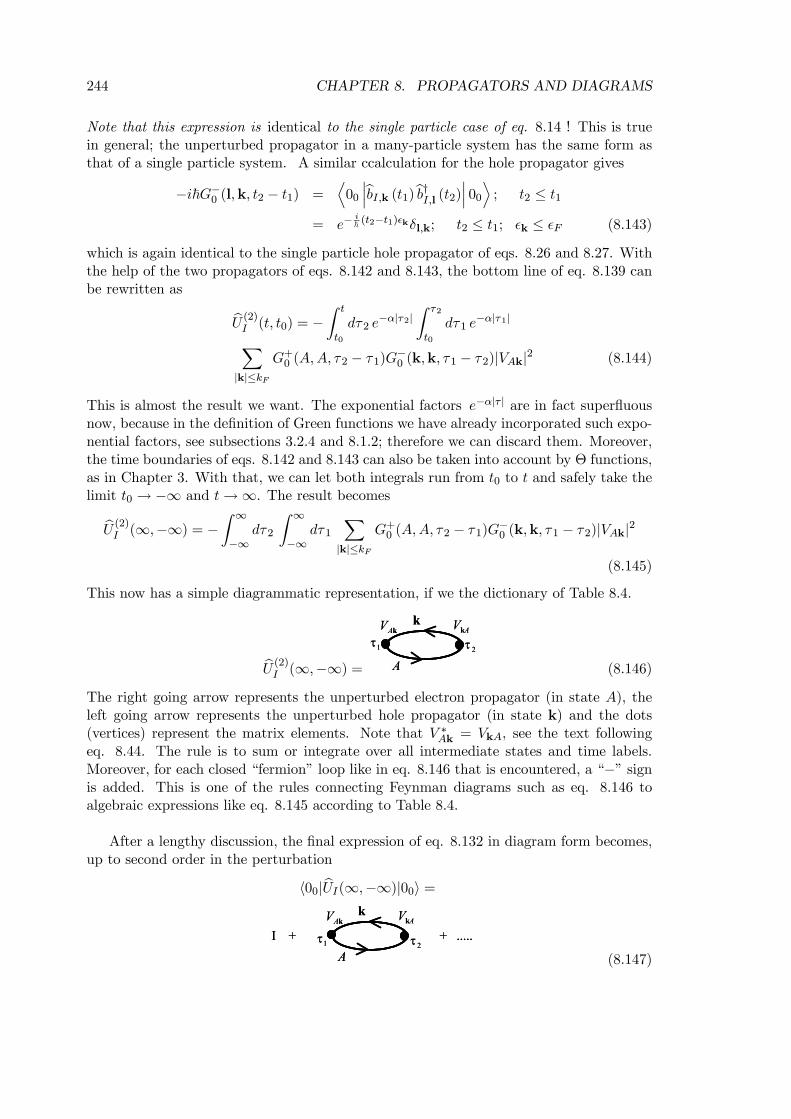
244 CHAPTER 8. PROPAGATORS AND DIAGRAMS
Note that this expression is identical to the single particle case of eq. 8.14 ! This is truein general; the unperturbed propagator in a many-particle system has the same form asthat of a single particle system. A similar ccalculation for the hole propagator gives
−i~G−0 (l,k, t2 − t1) =D00
¯bbI,k (t1)bb†I,l (t2)¯ 00E ; t2 ≤ t1= e−
i~ (t2−t1)²kδl,k; t2 ≤ t1; ²k ≤ ²F (8.143)
which is again identical to the single particle hole propagator of eqs. 8.26 and 8.27. Withthe help of the two propagators of eqs. 8.142 and 8.143, the bottom line of eq. 8.139 canbe rewritten as
bU (2)I (t, t0) = −Z t
t0
dτ2 e−α|τ2|
Z τ2
t0
dτ1 e−α|τ1|X
|k|≤kFG+0 (A,A, τ2 − τ1)G
−0 (k,k, τ1 − τ2)|VAk|2 (8.144)
This is almost the result we want. The exponential factors e−α|τ | are in fact superfluousnow, because in the definition of Green functions we have already incorporated such expo-nential factors, see subsections 3.2.4 and 8.1.2; therefore we can discard them. Moreover,the time boundaries of eqs. 8.142 and 8.143 can also be taken into account by Θ functions,as in Chapter 3. With that, we can let both integrals run from t0 to t and safely take thelimit t0 → −∞ and t→∞. The result becomesbU (2)I (∞,−∞) = −
Z ∞
−∞dτ2
Z ∞
−∞dτ1
X|k|≤kF
G+0 (A,A, τ2 − τ1)G−0 (k,k, τ1 − τ2)|VAk|2
(8.145)
This now has a simple diagrammatic representation, if we the dictionary of Table 8.4.
bU (2)I (∞,−∞) = A
k
1τkAV AVk
2τ
A
k
1τkAV AVk
2τ
(8.146)
The right going arrow represents the unperturbed electron propagator (in state A), theleft going arrow represents the unperturbed hole propagator (in state k) and the dots(vertices) represent the matrix elements. Note that V ∗Ak = VkA, see the text followingeq. 8.44. The rule is to sum or integrate over all intermediate states and time labels.Moreover, for each closed “fermion” loop like in eq. 8.146 that is encountered, a “−” signis added. This is one of the rules connecting Feynman diagrams such as eq. 8.146 toalgebraic expressions like eq. 8.145 according to Table 8.4.
After a lengthy discussion, the final expression of eq. 8.132 in diagram form becomes,up to second order in the perturbation
h00|bUI(∞,−∞)|00i =
A
k
I + + .....kAV AVk
1τ 2τA
k
I + + .....kAV AVk
1τ 2τ(8.147)
8.8. APPENDIX II. THE LINKED CLUSTER EXPANSION 245
The higher order terms can be derived systematically in a similar way. See whether youcan derive all fourth order terms yourself (and argue why there are no third order terms).
8.8.2 Numerator
Unfortunately, eq. 8.147 is just half the job we have to do. We still have to calculate thenumerator of the expression of eq. 8.131.
h00|bUI(∞, t2)baI,A(t2)bUI(t2, t1)ba†I,A(t1)bUI(t1,−∞)|00i (8.148)
This looks like a formidable expression, if we consider expanding each of the evolutionfactors bUI as a perturbation series as in eq. 8.132. However, things are somewhat lesshorrible than they seem at first sight. First of all, the expression for bVI (τ) which isneeded in the perturbation expansions is identical to eq. 8.45, if we substitute ba†A byba†I,A(τ), etcetera.
bVI(t) =X|k|>kF
³VkAba†I,k(t)baI,A(t) + VAkba†I,A(t)baI,k(t)´
+X|k|≤kF
³VkAbbI,k(t)baI,A(t) + VAkba†I,A(t)bb†I,k(t)´ (8.149)
This can easily be proven from eqs. 8.40 and 8.133. I have skipped the exponential factore−α|τ | now, because we have seen already that its main function is to let the time integralsin the perturbation series converge; from now on we will assume that they convergence.The time dependence of these creation and annihilation operators is rather simple
ba†I,A(t) = ba†Ae i~ t²A ; baI,A(t) = baAe− i~ t²A
ba†I,k(t) = ba†ke i~ t²k ; baI,k(t) = bake− i~ t²kbb†I,k(t) = bb†ke− i
~ t²k ; bbI,k(t) = bbke i~ t²k (8.150)
This can be proved straightforwardly.
ba†I,A(t)|0Ai = bU †0 (t, 0)ba†A bU0 (t, 0) |0Ai= e
i~ tbH0ba†Ae− i
~ tbH0 |0Ai = e i~ t bH0ba†Ae− i
~ tE0 |0Ai= e−
i~ tE0e
i~ tbH0ba†A|0Ai = e− i
~ tE0ei~ tbH0 |1Ai
= e−i~ tE0e
i~ t(E0+²A)|1Ai = e i~ t²Aba†A|0Ai
using eq. 8.40; see also the discussion around eq. 8.140. I have written the relation forthe state in which there are no electrons in the atomic state A, but it is easy to see that italso holds for all states with any numbers of particles or holes in the electron gas states.Therefore it is a property of the operator. The other relations in eq. 8.150 can be provenin a similar way.
A perturbation expansion of the evolution factors bUI in h00|....|00i, eq. 8.148, as in eq.8.132, leads to a string of creation and annihilation operators ...ba†I,k(t)baI,l(t)... between
246 CHAPTER 8. PROPAGATORS AND DIAGRAMS
the |....| . Let us start with the easy bits first. The zero’th order term is obtained bysetting all bUI = I in eq. 8.148. It gives the unperturbed propagation; compare eq. 8.46
h00|baI,A(t2)ba†I,A(t1)|00i = i~G+0 (A,A, t2 − t1) (8.151)
= 1tA
2tA
1tA
2tA
All possible first order terms give zero contributions. For instance look at the term
h00|baI,A(t2)ba†I,A(t1)bU (1)I (t1,−∞)|00i = h00|baI,A(t2)ba†I,A(t1) 1i~Z t1
−∞dτ1 bVI (τ1) |00i
= h00|baI,A(t2)ba†I,A(t1) 1i~Z t1
−∞dτ1
X|k|≤kF
VAkba†I,A(τ1)bb†I,k(τ1)|00i=
1
i~
Z t1
−∞dτ1
X|k|≤kF
VAkh00|baI,A(t2)ba†I,A(t1)ba†I,A(τ1)bb†I,k(τ1)|00i = 0 (8.152)
going from the first to the second line one observes that all the other terms in eq. bVI (τ)cannot contribute, since they try to annihilate a particle that is not present in the un-perturbed ground state, cf. eq. 8.149. However, looking at the third line of eq. 8.152one observes that it also must be zero, since ba†I,A(t1)ba†I,A(τ1) = 0. Because of the Pauliprinciple one cannot create two particles in the same state. One can argue even moreglobally whether a matrix element h00| bA|00i must be zero, where bA is some string of cre-ation and annihilation operators. Each creation operator increases the number of particles(or holes) by one and each annihilation operator decreases this number by one. The state|φi = bA|00i must contain zero particles and holes, otherwise h00|φi = h00| bA|00i = 0. Thismeans that each creation operator in the bA string has to be balanced by an annihilationoperator of the same kind and vice versa in order to give a non-zero overall result. In eq.8.152 the operator bb†I,k is not balanced by a bbI,k and one of the ba†I,A’s is not balanced by abaI,A. Therefore the overall result has to be zero. By a similar reasoning it is easy to showthat the other possible first order terms are also zero
h00|baI,A(t2)bU (1)I (t2, t1)ba†I,A(t1)|00i = h00|baI,A(t2) 1i~Z t2
t1
dτ1 bVI (τ1)ba†I,A(t1)|00i = 0(8.153)
h00|bU (1)I (∞, t2)baI,A(t2)ba†I,A(t1)|00i = h00| 1i~Z ∞
t2
dτ1 bVI (τ1)baI,A(t2)ba†I,A(t1)|00i = 0(8.154)
If one thinks this through, all perturbation terms which involve an odd number of bVI (τ)terms in h00|....|00i must be zero. It always gives a string of operators in which the
number of ba†A or the number of baA operators is unbalanced and such a string can nevergive a contribution when sandwiched between h00|....|00i.
8.8. APPENDIX II. THE LINKED CLUSTER EXPANSION 247
The even order terms are not zero a priori, so we have to work out in detail which ofthem give a contributiom. A possible second order term is
h00|baI,A(t2)ba†I,A(t1)bU (2)I (t1,−∞)|00i= h00|baI,A(t2)ba†I,A(t1)|00ih00|bU (2)I (t1,−∞)|00i (8.155)
In the second line we have inserted |00ih00|. You may wonder why we are allowed to dothat. We should actually insert a full resolution of identity
I =Xnk,nA
Yk
|nknAiYk
hnknA| (8.156)
where one sums over all possible states containing any number of particles and holes.However, operating with the product baI,A(t2)ba†I,A(t1) on each of these states does notchange the number of particles or holes. Taking the inner product h00|baI,A(t2)ba†I,A(t1) thenonly gives a non-zero contribution for the state with no particles or holes (i.e. the groundstate), since all the states with a different number of particles and holes are orthogonal
h00|Yk
|nknAi = 1 if all nk = nA = 0
= 0 otherwise (8.157)
We have calculated the two factors in the second line of eq. 8.155 before. Using eqs. 8.151and 8.145 one gets
h00|baI,A(t2)ba†I,A(t1)bU (2)I (t1,−∞)|00i = i~G+0 (A,A, t2 − t1)×
−Z t1
−∞dτ2
Z ∞
−∞dτ1
X|k|≤kF
G+0 (A,A, τ2 − τ1)G−0 (k,k, τ1 − τ2)|VAk|2 (8.158)
Note that we can let the time on the dτ1 integral run from −∞ to ∞ because G+0 andG−0 are zero anyway if τ1 > τ2. In a similar way one obtains for another possible secondorder term
h00|bU (2)I (∞, t2)baI,A(t2)ba†I,A(t1)|00i = i~G+0 (A,A, t2 − t1)×−Z ∞
t2
dτ2
Z ∞
−∞dτ1
X|k|≤kF
G+0 (A,A, τ2 − τ1)G−0 (k,k, τ1 − τ2)|VAk|2 (8.159)
Note that the only difference between the expression of eqs. 8.158 and 8.159 are the limitson the time integrals. The remaining second order term is
h00|baI,A(t2)bU (2)I (t2, t1)ba†I,A(t1)|00i= h00|baI,A(t2)µ 1
i~
¶2 Z t2
t1
dτ2
Z τ2
t1
dτ1 bVI (τ2) bVI (τ1)ba†I,A(t1)|00i=
µ1
i~
¶2 Z t2
t1
dτ2
Z τ2
t1
dτ1h00|baI,A(t2)bVI (τ2) bVI (τ1)ba†I,A(t1)|00i=
µ1
i~
¶2 Z t2
t1
dτ2
Z τ2
t1
dτ1X|k|>kF
VAkVkA
h00|baI,A(t2)ba†I,A(τ2)baI,k(τ2)ba†I,k(τ1)baI,A(τ1)ba†I,A(t1)|00i (8.160)
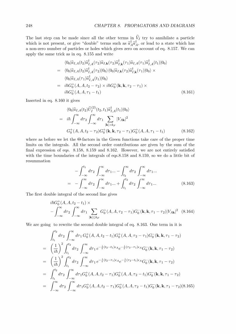
248 CHAPTER 8. PROPAGATORS AND DIAGRAMS
The last step can be made since all the other terms in bVI try to annihilate a particlewhich is not present, or give “double” terms such as ba†Aba†A, or lead to a state which hasa non-zero number of particles or holes which gives zero on account of eq. 8.157. We canapply the same trick as in eq. 8.155 and write
h00|baI,A(t2)ba†I,A(τ2)baI,k(τ2)ba†I,k(τ1)baI,A(τ1)ba†I,A(t1)|00i= h00|baI,A(t2)ba†I,A(τ2)|00ih00|baI,k(τ2)ba†I,k(τ1)|00i ×
h00|baI,A(τ1)ba†I,A(t1)|00i= i~G+0 (A,A, t2 − τ2)× i~G+0 (k,k, τ2 − τ1)×
i~G+0 (A,A, τ1 − t1) (8.161)
Inserted in eq. 8.160 it gives
h00|baI,A(t2)bU (2)I (t2, t1)ba†I,A(t1)|00i= i~
Z ∞
−∞dτ2
Z ∞
−∞dτ1
X|k|>kF
|VAk|2
G+0 (A,A, t2 − τ2)G+0 (k,k, τ2 − τ1)G
+0 (A,A, τ1 − t1) (8.162)
where as before we let the Θ-factors in the Green functions take care of the proper timelimits on the integrals. All the second order contributions are given by the sum of thefinal expression of eqs. 8.158, 8.159 and 8.162. However, we are not entirely satisfiedwith the time boundaries of the integrals of eqs.8.158 and 8.159, so we do a little bit ofresummation
−Z t1
−∞dτ2
Z ∞
−∞dτ1...−
Z ∞
t2
dτ2
Z ∞
−∞dτ1...
= −Z ∞
−∞dτ2
Z ∞
−∞dτ1...+
Z t2
t1
dτ2
Z ∞
−∞dτ1... (8.163)
The first double integral of the second line gives
i~G+0 (A,A, t2 − t1)×−Z ∞
−∞dτ2
Z ∞
−∞dτ1
X|k|≤kF
G+0 (A,A, τ2 − τ1)G−0 (k,k, τ1 − τ2)|VAk|2 (8.164)
We are going to rewrite the second double integral of eq. 8.163. One term in it isZ t2
t1
dτ2
Z ∞
−∞dτ1G
+0 (A,A, t2 − t1)G+0 (A,A, τ2 − τ1)G
−0 (k,k, τ1 − τ2)
=
µ1
i~
¶2 Z t2
t1
dτ2
Z ∞
−∞dτ1 e
− i~ (t2−t1)²Ae−
i~ (τ2−τ1)²AG−0 (k,k, τ1 − τ2)
=
µ1
i~
¶2 Z t2
t1
dτ2
Z ∞
−∞dτ1 e
− i~ (t2−τ1)²Ae−
i~ (τ2−t1)²AG−0 (k,k, τ1 − τ2)
=
Z t2
t1
dτ2
Z ∞
−∞dτ1G
+0 (A,A, t2 − τ1)G
+0 (A,A, τ2 − t1)G−0 (k,k, τ1 − τ2)
=
Z ∞
−∞dτ2
Z ∞
−∞dτ1G
+0 (A,A, t2 − τ1)G
+0 (A,A, τ2 − t1)G−0 (k,k, τ1 − τ2)(8.165)
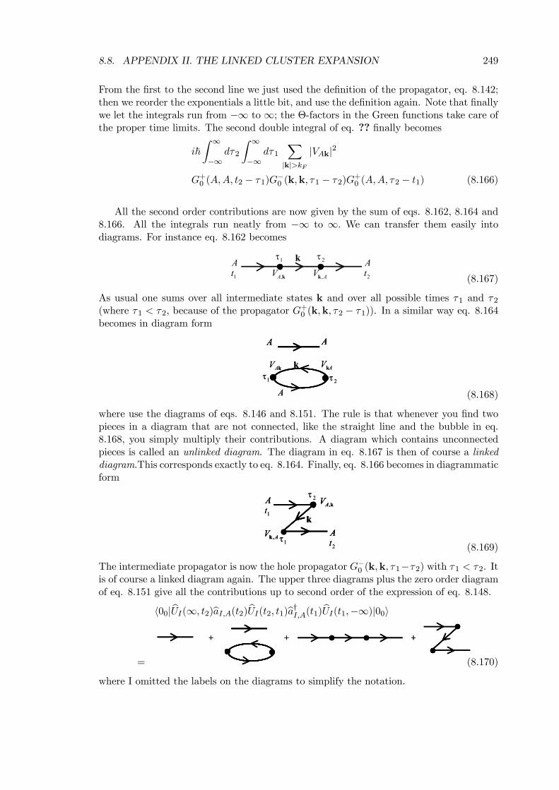
8.8. APPENDIX II. THE LINKED CLUSTER EXPANSION 249
From the first to the second line we just used the definition of the propagator, eq. 8.142;then we reorder the exponentials a little bit, and use the definition again. Note that finallywe let the integrals run from −∞ to ∞; the Θ-factors in the Green functions take care ofthe proper time limits. The second double integral of eq. ?? finally becomes
i~Z ∞
−∞dτ2
Z ∞
−∞dτ1
X|k|>kF
|VAk|2
G+0 (A,A, t2 − τ1)G−0 (k,k, τ1 − τ2)G
+0 (A,A, τ2 − t1) (8.166)
All the second order contributions are now given by the sum of eqs. 8.162, 8.164 and8.166. All the integrals run neatly from −∞ to ∞. We can transfer them easily intodiagrams. For instance eq. 8.162 becomes
A Ak
k,AV AV ,k1t 2t1τ 2τ
(8.167)
As usual one sums over all intermediate states k and over all possible times τ1 and τ2(where τ1 < τ2, because of the propagator G
+0 (k,k, τ2 − τ1)). In a similar way eq. 8.164
becomes in diagram form
A
k1τ
kAV AVk2τ
A A
A
k1τ
kAV AVk2τ
A AA A
(8.168)
where use the diagrams of eqs. 8.146 and 8.151. The rule is that whenever you find twopieces in a diagram that are not connected, like the straight line and the bubble in eq.8.168, you simply multiply their contributions. A diagram which contains unconnectedpieces is called an unlinked diagram. The diagram in eq. 8.167 is then of course a linkeddiagram.This corresponds exactly to eq. 8.164. Finally, eq. 8.166 becomes in diagrammaticform
A k,AV
AV ,k
kA
1t
2t1τ
2τA k,AV
AV ,k
kA
A k,AV
AV ,k
kA
1t
2t1τ
2τ
(8.169)
The intermediate propagator is now the hole propagator G−0 (k,k, τ1−τ2) with τ1 < τ2. Itis of course a linked diagram again. The upper three diagrams plus the zero order diagramof eq. 8.151 give all the contributions up to second order of the expression of eq. 8.148.
h00|bUI(∞, t2)baI,A(t2)bUI(t2, t1)ba†I,A(t1)bUI(t1,−∞)|00i
=
+ ++ + ++ +++
(8.170)
where I omitted the labels on the diagrams to simplify the notation.
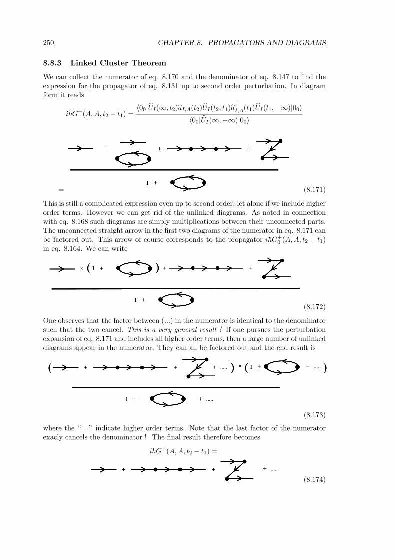
250 CHAPTER 8. PROPAGATORS AND DIAGRAMS
8.8.3 Linked Cluster Theorem
We can collect the numerator of eq. 8.170 and the denominator of eq. 8.147 to find theexpression for the propagator of eq. 8.131 up to second order perturbation. In diagramform it reads
i~G+(A,A, t2 − t1) =h00|bUI(∞, t2)baI,A(t2)bUI(t2, t1)ba†I,A(t1)bUI(t1,−∞)|00i
h00|bUI(∞,−∞)|00i
=
+ ++
I +
+ ++ + ++ +++
I +I +(8.171)
This is still a complicated expression even up to second order, let alone if we include higherorder terms. However we can get rid of the unlinked diagrams. As noted in connectionwith eq. 8.168 such diagrams are simply multiplications between their unconnected parts.The unconnected straight arrow in the first two diagrams of the numerator in eq. 8.171 canbe factored out. This arrow of course corresponds to the propagator i~G+0 (A,A, t2 − t1)in eq. 8.164. We can write
× +
I +
I +( ) +× +
I +
I +( ) +
(8.172)
One observes that the factor between (...) in the numerator is identical to the denominatorsuch that the two cancel. This is a very general result ! If one pursues the perturbationexpansion of eq. 8.171 and includes all higher order terms, then a large number of unlinkeddiagrams appear in the numerator. They can all be factored out and the end result is
I + + .....
+ +( ) × ( )I + + .....+ .....
I + + .....
+ +( ) × ( )I + + .....+ .....
(8.173)
where the “....” indicate higher order terms. Note that the last factor of the numeratorexacly cancels the denominator ! The final result therefore becomes
i~G+(A,A, t2 − t1) =
+ + + .....+ ++ + + .....
(8.174)
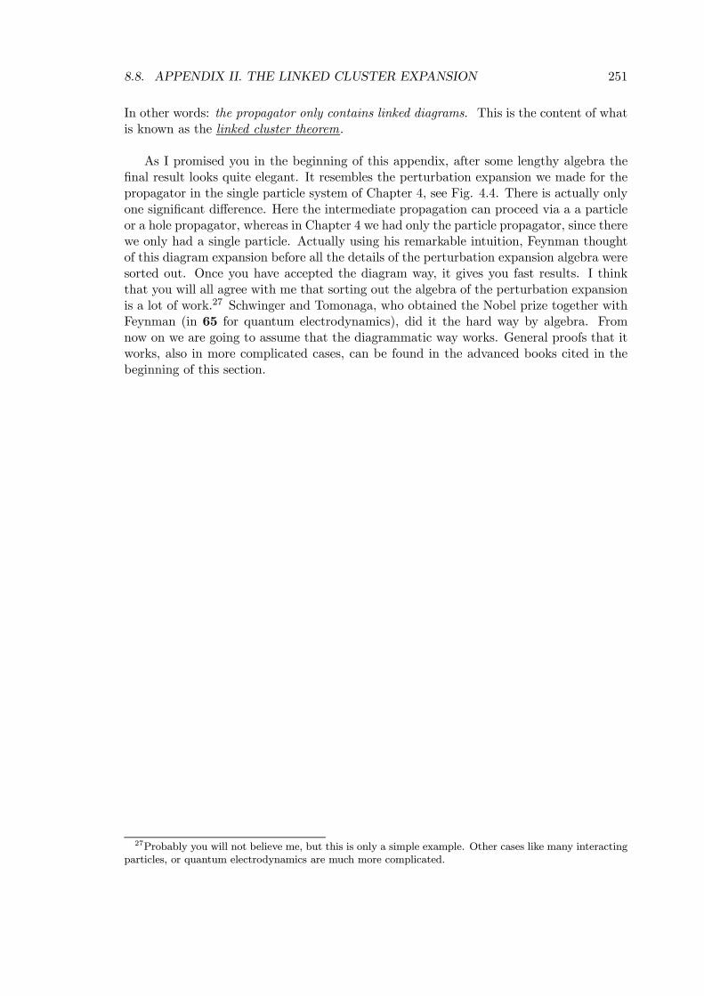
8.8. APPENDIX II. THE LINKED CLUSTER EXPANSION 251
In other words: the propagator only contains linked diagrams. This is the content of whatis known as the linked cluster theorem.
As I promised you in the beginning of this appendix, after some lengthy algebra thefinal result looks quite elegant. It resembles the perturbation expansion we made for thepropagator in the single particle system of Chapter 4, see Fig. 4.4. There is actually onlyone significant difference. Here the intermediate propagation can proceed via a a particleor a hole propagator, whereas in Chapter 4 we had only the particle propagator, since therewe only had a single particle. Actually using his remarkable intuition, Feynman thoughtof this diagram expansion before all the details of the perturbation expansion algebra weresorted out. Once you have accepted the diagram way, it gives you fast results. I thinkthat you will all agree with me that sorting out the algebra of the perturbation expansionis a lot of work.27 Schwinger and Tomonaga, who obtained the Nobel prize together withFeynman (in 65 for quantum electrodynamics), did it the hard way by algebra. Fromnow on we are going to assume that the diagrammatic way works. General proofs that itworks, also in more complicated cases, can be found in the advanced books cited in thebeginning of this section.
27Probably you will not believe me, but this is only a simple example. Other cases like many interactingparticles, or quantum electrodynamics are much more complicated.

252 CHAPTER 8. PROPAGATORS AND DIAGRAMS
Chapter 9
The electron-electron interaction
“It seems very pretty,” she said when she had finished it, “but it’s rather hard to understand!”
(You see she didn’t like to confess even to herself, that she couldn’t make it out at all.) “Somehow it
seems to fill my head with ideas—only I don’t exactly know what they are!”, Lewis Carrol, Through
the Looking Glass.
9.1 Many interacting electrons
As in the previous chapter, our focus is on the one particle propagator and the gedanken-experiment it represents. For particles it reads, cf. eq. 8.7,
i~G+(m,k, t2 − t1) =D0¯bak (t2)ba†m (t1)¯ 0E (9.1)
There is however a snake in the grass; the vacuum state |0i is the ground state of theinteracting electron gas and we complained before about not being able to find solutions(including the ground state) for the interacting electron gas. However, the “adiabaticconnection” and the “linked cluster expansion” discussed in the appendices of the previouschapter ensure that the diagrammatic techniques we are going to use also work in thiscase. From now on we will assume they do. As before the propagator gives the probabilityamplitude of finding a particle in a statem at a time t2, after it has been created in a statek at a time t1. It represents a gedanken experiment, but real experiments like (inverse)photoemission are closely connected to it.
As for the non-interacting electron gas, we approach the problem by rewriting eq. 9.1in terms of time-evolution operators and making a time-dependent perturbation seriesexpansion. For the interacting case, the mathematics is much more involved. We willignore this completely and handle the diagrams just as in the non-interacting case (whichis correct). The “unperturbed” Hamiltonian bH0 is taken to be the kinetic energy plus anyatomic potentials present of the type of eq. 8.77.1 The two-particle interaction bV of eq.8.81 is now treated as the perturbation. Since this represents a Coulomb repulsion, whichby comparing eqs. 8.75 and 8.80 one expects to be of a similar order of magnitude as theattraction by the atomic potentials, the perturbation will not be small. On forehand one
1In a homogeneous electron gas there is only the kinetic energy off course.
253
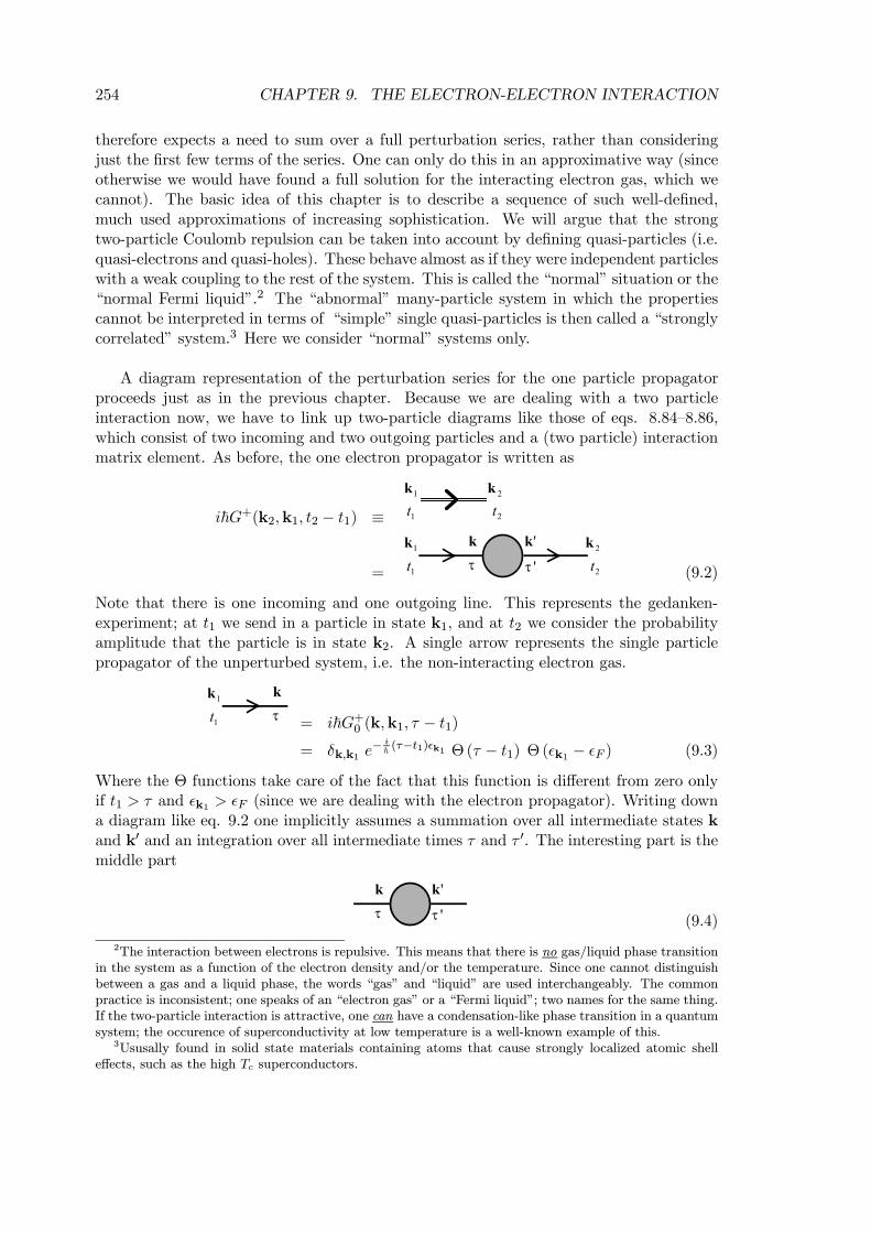
254 CHAPTER 9. THE ELECTRON-ELECTRON INTERACTION
therefore expects a need to sum over a full perturbation series, rather than consideringjust the first few terms of the series. One can only do this in an approximative way (sinceotherwise we would have found a full solution for the interacting electron gas, which wecannot). The basic idea of this chapter is to describe a sequence of such well-defined,much used approximations of increasing sophistication. We will argue that the strongtwo-particle Coulomb repulsion can be taken into account by defining quasi-particles (i.e.quasi-electrons and quasi-holes). These behave almost as if they were independent particleswith a weak coupling to the rest of the system. This is called the “normal” situation or the“normal Fermi liquid”.2 The “abnormal” many-particle system in which the propertiescannot be interpreted in terms of “simple” single quasi-particles is then called a “stronglycorrelated” system.3 Here we consider “normal” systems only.
A diagram representation of the perturbation series for the one particle propagatorproceeds just as in the previous chapter. Because we are dealing with a two particleinteraction now, we have to link up two-particle diagrams like those of eqs. 8.84—8.86,which consist of two incoming and two outgoing particles and a (two particle) interactionmatrix element. As before, the one electron propagator is written as
i~G+(k2,k1, t2 − t1) ≡ 2t1t1k 2k
= 2t1t1k 2k
τ
k
'τ
'k
(9.2)
Note that there is one incoming and one outgoing line. This represents the gedanken-experiment; at t1 we send in a particle in state k1, and at t2 we consider the probabilityamplitude that the particle is in state k2. A single arrow represents the single particlepropagator of the unperturbed system, i.e. the non-interacting electron gas.
1t1k
τ
k
= i~G+0 (k,k1, τ − t1)= δk,k1 e
− i~ (τ−t1)²k1 Θ (τ − t1) Θ (²k1 − ²F ) (9.3)
Where the Θ functions take care of the fact that this function is different from zero onlyif t1 > τ and ²k1 > ²F (since we are dealing with the electron propagator). Writing downa diagram like eq. 9.2 one implicitly assumes a summation over all intermediate states kand k0 and an integration over all intermediate times τ and τ 0. The interesting part is themiddle part
τ
k
'τ
'k
(9.4)
2The interaction between electrons is repulsive. This means that there is no gas/liquid phase transitionin the system as a function of the electron density and/or the temperature. Since one cannot distinguishbetween a gas and a liquid phase, the words “gas” and “liquid” are used interchangeably. The commonpractice is inconsistent; one speaks of an “electron gas” or a “Fermi liquid”; two names for the same thing.If the two-particle interaction is attractive, one can have a condensation-like phase transition in a quantumsystem; the occurence of superconductivity at low temperature is a well-known example of this.
3Ususally found in solid state materials containing atoms that cause strongly localized atomic shelleffects, such as the high Tc superconductors.
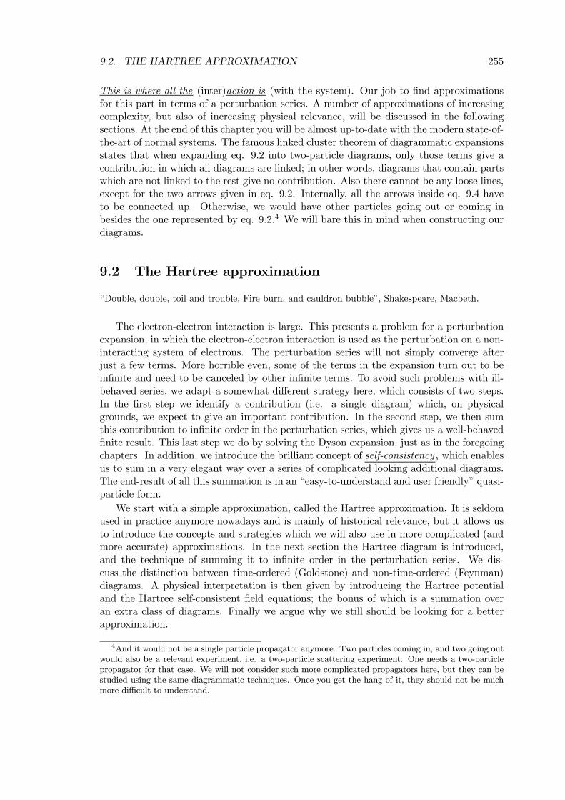
9.2. THE HARTREE APPROXIMATION 255
This is where all the (inter)action is (with the system). Our job to find approximationsfor this part in terms of a perturbation series. A number of approximations of increasingcomplexity, but also of increasing physical relevance, will be discussed in the followingsections. At the end of this chapter you will be almost up-to-date with the modern state-of-the-art of normal systems. The famous linked cluster theorem of diagrammatic expansionsstates that when expanding eq. 9.2 into two-particle diagrams, only those terms give acontribution in which all diagrams are linked; in other words, diagrams that contain partswhich are not linked to the rest give no contribution. Also there cannot be any loose lines,except for the two arrows given in eq. 9.2. Internally, all the arrows inside eq. 9.4 haveto be connected up. Otherwise, we would have other particles going out or coming inbesides the one represented by eq. 9.2.4 We will bare this in mind when constructing ourdiagrams.
9.2 The Hartree approximation
“Double, double, toil and trouble, Fire burn, and cauldron bubble”, Shakespeare, Macbeth.
The electron-electron interaction is large. This presents a problem for a perturbationexpansion, in which the electron-electron interaction is used as the perturbation on a non-interacting system of electrons. The perturbation series will not simply converge afterjust a few terms. More horrible even, some of the terms in the expansion turn out to beinfinite and need to be canceled by other infinite terms. To avoid such problems with ill-behaved series, we adapt a somewhat different strategy here, which consists of two steps.In the first step we identify a contribution (i.e. a single diagram) which, on physicalgrounds, we expect to give an important contribution. In the second step, we then sumthis contribution to infinite order in the perturbation series, which gives us a well-behavedfinite result. This last step we do by solving the Dyson expansion, just as in the foregoingchapters. In addition, we introduce the brilliant concept of self-consistency, which enablesus to sum in a very elegant way over a series of complicated looking additional diagrams.The end-result of all this summation is in an “easy-to-understand and user friendly” quasi-particle form.
We start with a simple approximation, called the Hartree approximation. It is seldomused in practice anymore nowadays and is mainly of historical relevance, but it allows usto introduce the concepts and strategies which we will also use in more complicated (andmore accurate) approximations. In the next section the Hartree diagram is introduced,and the technique of summing it to infinite order in the perturbation series. We dis-cuss the distinction between time-ordered (Goldstone) and non-time-ordered (Feynman)diagrams. A physical interpretation is then given by introducing the Hartree potentialand the Hartree self-consistent field equations; the bonus of which is a summation overan extra class of diagrams. Finally we argue why we still should be looking for a betterapproximation.
4And it would not be a single particle propagator anymore. Two particles coming in, and two going outwould also be a relevant experiment, i.e. a two-particle scattering experiment. One needs a two-particlepropagator for that case. We will not consider such more complicated propagators here, but they can bestudied using the same diagrammatic techniques. Once you get the hang of it, they should not be muchmore difficult to understand.
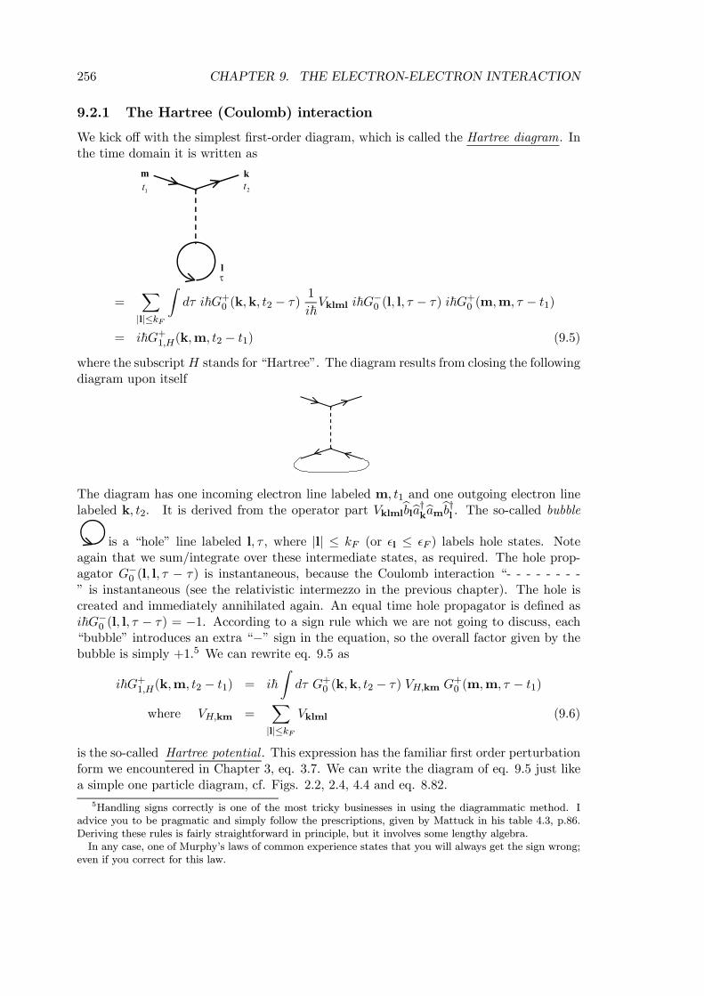
256 CHAPTER 9. THE ELECTRON-ELECTRON INTERACTION
9.2.1 The Hartree (Coulomb) interaction
We kick off with the simplest first-order diagram, which is called the Hartree diagram. Inthe time domain it is written as
l
km1t 2t
τ
=X|l|≤kF
Zdτ i~G+0 (k,k, t2 − τ)
1
i~Vklml i~G−0 (l, l, τ − τ) i~G+0 (m,m, τ − t1)
= i~G+1,H(k,m, t2 − t1) (9.5)
where the subscriptH stands for “Hartree”. The diagram results from closing the followingdiagram upon itself
The diagram has one incoming electron line labeled m, t1 and one outgoing electron linelabeled k, t2. It is derived from the operator part Vklmlbblba†kbambb†l . The so-called bubble
is a “hole” line labeled l, τ , where |l| ≤ kF (or ²l ≤ ²F ) labels hole states. Noteagain that we sum/integrate over these intermediate states, as required. The hole prop-agator G−0 (l, l, τ − τ) is instantaneous, because the Coulomb interaction “- - - - - - - -” is instantaneous (see the relativistic intermezzo in the previous chapter). The hole iscreated and immediately annihilated again. An equal time hole propagator is defined asi~G−0 (l, l, τ − τ) = −1. According to a sign rule which we are not going to discuss, each“bubble” introduces an extra “−” sign in the equation, so the overall factor given by thebubble is simply +1.5 We can rewrite eq. 9.5 as
i~G+1,H(k,m, t2 − t1) = i~Zdτ G+0 (k,k, t2 − τ) VH,km G
+0 (m,m, τ − t1)
where VH,km =X|l|≤kF
Vklml (9.6)
is the so-called Hartree potential . This expression has the familiar first order perturbationform we encountered in Chapter 3, eq. 3.7. We can write the diagram of eq. 9.5 just likea simple one particle diagram, cf. Figs. 2.2, 2.4, 4.4 and eq. 8.82.
5Handling signs correctly is one of the most tricky businesses in using the diagrammatic method. Iadvice you to be pragmatic and simply follow the prescriptions, given by Mattuck in his table 4.3, p.86.Deriving these rules is fairly straightforward in principle, but it involves some lengthy algebra.In any case, one of Murphy’s laws of common experience states that you will always get the sign wrong;
even if you correct for this law.
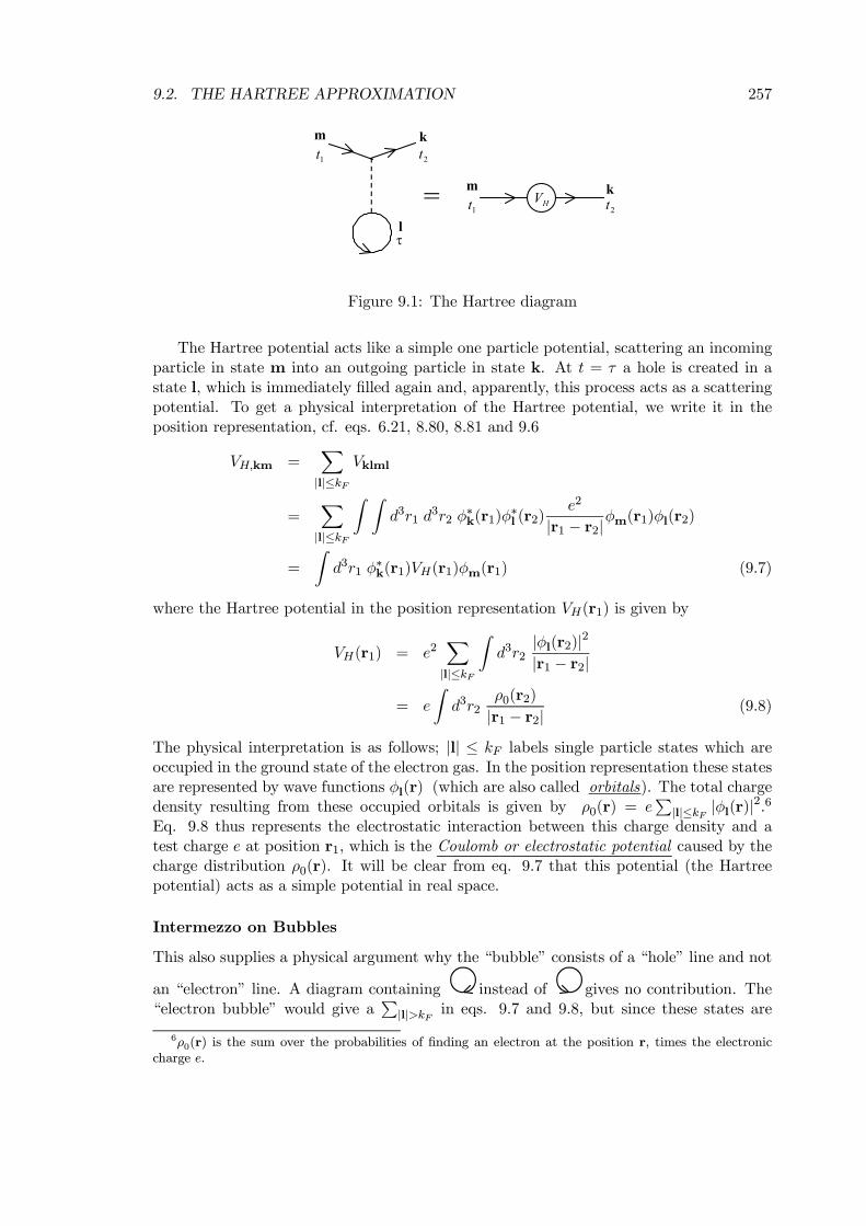
9.2. THE HARTREE APPROXIMATION 257
l
km1t 2t
τ
= HVm
1tk
2t
Figure 9.1: The Hartree diagram
The Hartree potential acts like a simple one particle potential, scattering an incomingparticle in state m into an outgoing particle in state k. At t = τ a hole is created in astate l, which is immediately filled again and, apparently, this process acts as a scatteringpotential. To get a physical interpretation of the Hartree potential, we write it in theposition representation, cf. eqs. 6.21, 8.80, 8.81 and 9.6
VH,km =X|l|≤kF
Vklml
=X|l|≤kF
Z Zd3r1 d
3r2 φ∗k(r1)φ
∗l (r2)
e2
|r1 − r2|φm(r1)φl(r2)
=
Zd3r1 φ
∗k(r1)VH(r1)φm(r1) (9.7)
where the Hartree potential in the position representation VH(r1) is given by
VH(r1) = e2X|l|≤kF
Zd3r2
|φl(r2)|2|r1 − r2|
= e
Zd3r2
ρ0(r2)
|r1 − r2| (9.8)
The physical interpretation is as follows; |l| ≤ kF labels single particle states which areoccupied in the ground state of the electron gas. In the position representation these statesare represented by wave functions φl(r) (which are also called orbitals). The total chargedensity resulting from these occupied orbitals is given by ρ0(r) = e
P|l|≤kF |φl(r)|
2.6
Eq. 9.8 thus represents the electrostatic interaction between this charge density and atest charge e at position r1, which is the Coulomb or electrostatic potential caused by thecharge distribution ρ0(r). It will be clear from eq. 9.7 that this potential (the Hartreepotential) acts as a simple potential in real space.
Intermezzo on Bubbles
This also supplies a physical argument why the “bubble” consists of a “hole” line and not
an “electron” line. A diagram containing instead of gives no contribution. The“electron bubble” would give a
P|l|>kF in eqs. 9.7 and 9.8, but since these states are
6ρ0(r) is the sum over the probabilities of finding an electron at the position r, times the electroniccharge e.
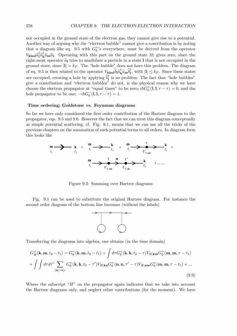
258 CHAPTER 9. THE ELECTRON-ELECTRON INTERACTION
not occupied in the ground state of the electron gas, they cannot give rise to a potential.Another way of arguing why the “electron bubble” cannot give a contribution is by notingthat a diagram like eq. 9.5 with G+0 ’s everywhere, must be derived from the operator
Vklmlba†lba†kbambal. Operating with this part on the ground state |0i gives zero, since theright-most operator bal tries to annihilate a particle in a state l that is not occupied in theground state, since |l| > kF . The “hole bubble” does not have this problem. The diagramof eq. 9.5 is then related to the operator Vklmlbblba†kbambb†l , with |l| ≤ kF . Since these statesare occupied, creating a hole by applying bb†l is no problem. The fact that “hole bubbles”give a contribution and “electron bubbles” do not, is the physical reason why we havechoose the electron propagator at “equal times” to be zero; i~G+0 (l, l, τ − τ) = 0, and thehole propagator to be one; −i~G−0 (l, l, τ − τ) = 1.
Time ordering; Goldstone vs. Feynman diagrams
So far we have only considered the first order contribution of the Hartree diagram to thepropagator, eqs. 9.5 and 9.6. However the fact that we can treat this diagram conceptuallyas simple potential scattering, cf. Fig. 9.1, means that we can use all the tricks of theprevious chapters on the summation of such potential terms to all orders. In diagram formthis looks like
= +mk,HV
+
n........+
mn,HV nk,HV
m1t
k2t
m1t
m1t
m1t
k2t
k2t
k2t
τ
τ 'τ
Figure 9.2: Summing over Hartree diagrams
Fig. 9.1 can be used to substitute the original Hartree diagram. For instance thesecond order diagram of the bottom line becomes (without the labels)
Transferring the diagrams into algebra, one obtains (in the time domain)
G+H(k,m, t2 − t1) = G+0 (k,m, t2 − t1) +ZdτG+0 (k,k, t2 − τ)VH,kmG
+0 (m,m, τ − t1)
+
Z Zdτdτ 0
X|n|>kF
G+0 (k,k, t2 − τ 0)VH,knG+0 (n,n, τ0 − τ)VH,nmG
+0 (m,m, τ − t1) + ...
(9.9)
Where the subscript “H” on the propagator again indicates that we take into accountthe Hartree diagrams only, and neglect other contributions (for the moment). We have
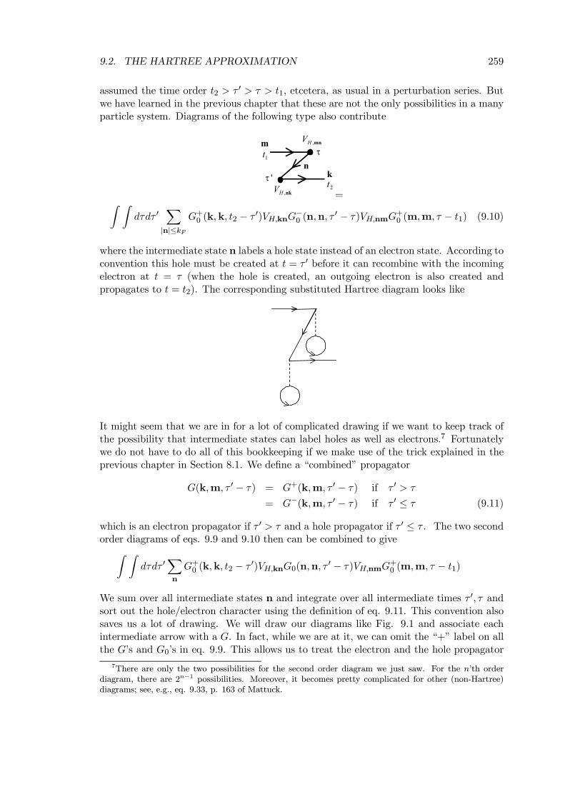
9.2. THE HARTREE APPROXIMATION 259
assumed the time order t2 > τ 0 > τ > t1, etcetera, as usual in a perturbation series. Butwe have learned in the previous chapter that these are not the only possibilities in a manyparticle system. Diagrams of the following type also contribute
m1t
mn,HVτ
nk,HV'τ k
2t
n
=Z Zdτdτ 0
X|n|≤kF
G+0 (k,k, t2 − τ 0)VH,knG−0 (n,n, τ0 − τ)VH,nmG
+0 (m,m, τ − t1) (9.10)
where the intermediate state n labels a hole state instead of an electron state. According toconvention this hole must be created at t = τ 0 before it can recombine with the incomingelectron at t = τ (when the hole is created, an outgoing electron is also created andpropagates to t = t2). The corresponding substituted Hartree diagram looks like
It might seem that we are in for a lot of complicated drawing if we want to keep track ofthe possibility that intermediate states can label holes as well as electrons.7 Fortunatelywe do not have to do all of this bookkeeping if we make use of the trick explained in theprevious chapter in Section 8.1. We define a “combined” propagator
G(k,m, τ 0 − τ) = G+(k,m, τ 0 − τ) if τ 0 > τ
= G−(k,m, τ 0 − τ) if τ 0 ≤ τ (9.11)
which is an electron propagator if τ 0 > τ and a hole propagator if τ 0 ≤ τ . The two secondorder diagrams of eqs. 9.9 and 9.10 then can be combined to giveZ Z
dτdτ 0Xn
G+0 (k,k, t2 − τ 0)VH,knG0(n,n, τ 0 − τ)VH,nmG+0 (m,m, τ − t1)
We sum over all intermediate states n and integrate over all intermediate times τ 0, τ andsort out the hole/electron character using the definition of eq. 9.11. This convention alsosaves us a lot of drawing. We will draw our diagrams like Fig. 9.1 and associate eachintermediate arrow with a G. In fact, while we are at it, we can omit the “+” label on allthe G’s and G0’s in eq. 9.9. This allows us to treat the electron and the hole propagator
7There are only the two possibilities for the second order diagram we just saw. For the n’th orderdiagram, there are 2n−1 possibilities. Moreover, it becomes pretty complicated for other (non-Hartree)diagrams; see, e.g., eq. 9.33, p. 163 of Mattuck.
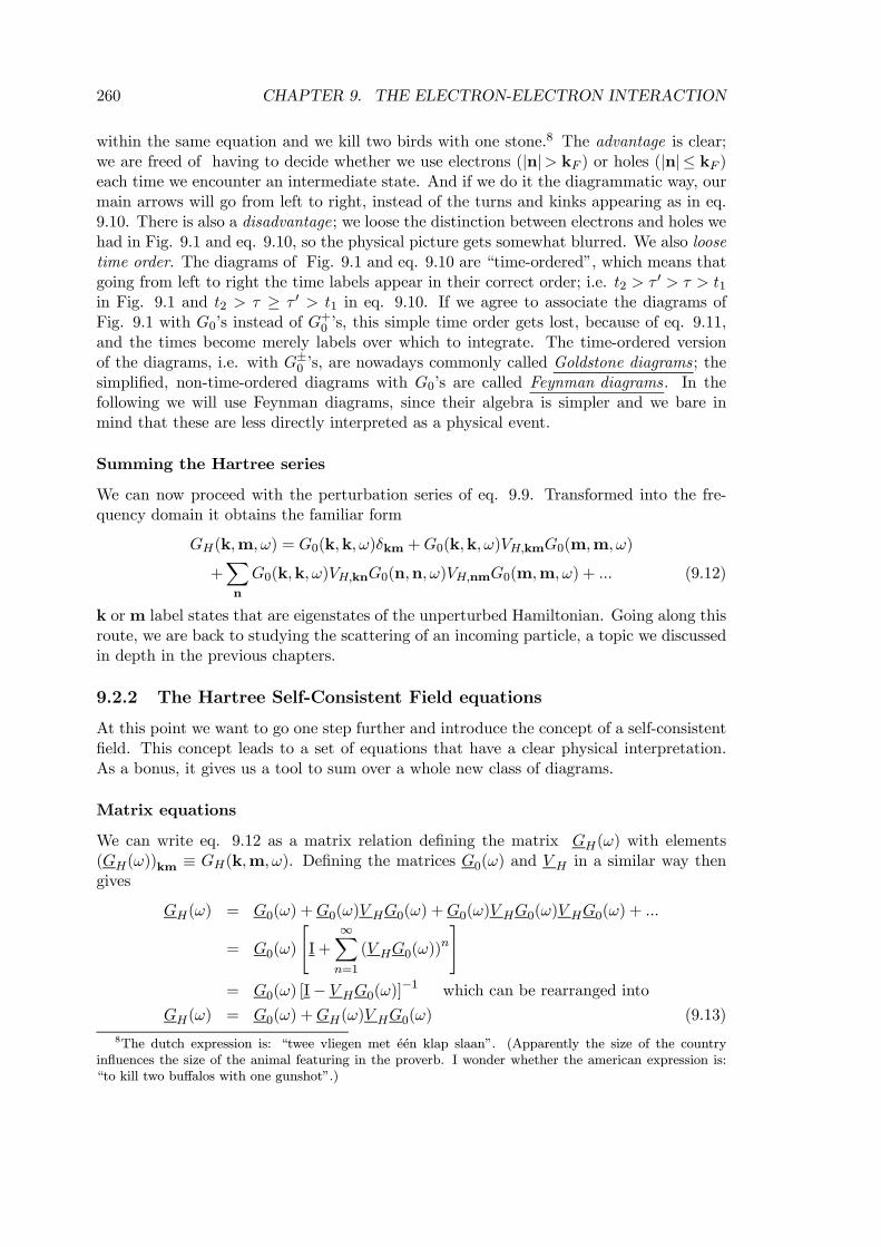
260 CHAPTER 9. THE ELECTRON-ELECTRON INTERACTION
within the same equation and we kill two birds with one stone.8 The advantage is clear;we are freed of having to decide whether we use electrons (|n|> kF ) or holes (|n|≤ kF )each time we encounter an intermediate state. And if we do it the diagrammatic way, ourmain arrows will go from left to right, instead of the turns and kinks appearing as in eq.9.10. There is also a disadvantage; we loose the distinction between electrons and holes wehad in Fig. 9.1 and eq. 9.10, so the physical picture gets somewhat blurred. We also loosetime order. The diagrams of Fig. 9.1 and eq. 9.10 are “time-ordered”, which means thatgoing from left to right the time labels appear in their correct order; i.e. t2 > τ 0 > τ > t1in Fig. 9.1 and t2 > τ ≥ τ 0 > t1 in eq. 9.10. If we agree to associate the diagrams ofFig. 9.1 with G0’s instead of G
+0 ’s, this simple time order gets lost, because of eq. 9.11,
and the times become merely labels over which to integrate. The time-ordered versionof the diagrams, i.e. with G±0 ’s, are nowadays commonly called Goldstone diagrams; thesimplified, non-time-ordered diagrams with G0’s are called Feynman diagrams. In thefollowing we will use Feynman diagrams, since their algebra is simpler and we bare inmind that these are less directly interpreted as a physical event.
Summing the Hartree series
We can now proceed with the perturbation series of eq. 9.9. Transformed into the fre-quency domain it obtains the familiar form
GH(k,m,ω) = G0(k,k,ω)δkm +G0(k,k,ω)VH,kmG0(m,m,ω)
+Xn
G0(k,k,ω)VH,knG0(n,n,ω)VH,nmG0(m,m,ω) + ... (9.12)
k orm label states that are eigenstates of the unperturbed Hamiltonian. Going along thisroute, we are back to studying the scattering of an incoming particle, a topic we discussedin depth in the previous chapters.
9.2.2 The Hartree Self-Consistent Field equations
At this point we want to go one step further and introduce the concept of a self-consistentfield. This concept leads to a set of equations that have a clear physical interpretation.As a bonus, it gives us a tool to sum over a whole new class of diagrams.
Matrix equations
We can write eq. 9.12 as a matrix relation defining the matrix GH(ω) with elements(GH(ω))km ≡ GH(k,m,ω). Defining the matrices G0(ω) and V H in a similar way thengives
GH(ω) = G0(ω) +G0(ω)V HG0(ω) +G0(ω)V HG0(ω)V HG0(ω) + ...
= G0(ω)
"I +
∞Xn=1
(V HG0(ω))n
#= G0(ω) [I− V HG0(ω)]−1 which can be rearranged into
GH(ω) = G0(ω) +GH(ω)V HG0(ω) (9.13)
8The dutch expression is: “twee vliegen met een klap slaan”. (Apparently the size of the countryinfluences the size of the animal featuring in the proverb. I wonder whether the american expression is:“to kill two buffalos with one gunshot”.)
9.2. THE HARTREE APPROXIMATION 261
which is the familiar Dyson equation again. Remember
(G0(ω))km = G0(k,k,ω)δkm =1
~ω − ²0,k ± iδ δkm (9.14)
where ²0,k are the eigenvalues of the unperturbed Hamiltonian bH0 an the ±iδ is for elec-trons and holes respectively. Defining the obvious diagonal matrix (H0)km ≡ H0,km =²0,kδkm one gets
(G0(ω))km =³(~ω −H0 ± iδ)−1
´km
which gives
G0(ω)−1 = ~ω −H0 ± iδ (9.15)
The “−1” superscript means a matrix inversion now.9 Multiplying the left- and right-handside of eq. 9.13 with G0(ω)
−1 (from the right), rearranging the terms, and using eq. 9.15finally gives
(~ω −H0 − V H ± iδ)GH(ω) = I⇔GH(ω) = (~ω −H0 − V H ± iδ)−1 (9.16)
This equation now shows explicitly that the propagator GH in the Hartree approximationis the Green function (or Green matrix) associated with the Hamiltonian H0 + V H , inwhich the Hartree potential acts as an (extra) potential term.
Transform the basis set
We can make life simpler if we transform to eigenstates of this Hamiltonian. Define a newbasis set of one particle states |mHi, obtained by a linear transformation from the old set|ki (which are the single particle eigenstates of bH0 )
|mHi =Xk
|kiCkm or in wave function notation
ψm(r) =Xk
φk(r)Ckm (9.17)
where, as usual, ψm(r) = hr|mHi and φk(r) = hr|ki. Define a (column) vector |mHi theelements of which are |mHi, where mH runs over the whole basis. Eq. 9.17 then becomesin this notation
|mHi = CT |ki= C−1|ki (9.18)
Note that¡CT¢mk
= Ckm, as required. The last line follows because we wish our newbasis to be orthonormal, as was our old basis; an elementary theorem in linear algebrastates that the transformation between two orthonormal basis sets has to be unitary, andthus CT = C−1. Follow the linear algebra path. If A is a matrix represented on thebasis |ki, and AH is supposed to represent the same quantity on the basis |mHi and if
9In fact I should have written ~ωI with I the identity matrix, instead of ~ω,but I don’t want to complicatethe notation too much. For the same reason, if you are mathematically strict, read iδI instead of iδ.
262 CHAPTER 9. THE ELECTRON-ELECTRON INTERACTION
the transformation between the bases is given by eq. 9.18, then AH = C−1AC. We now
choose a very special transformation, namely the one which makes the “Hamiltonian”H0 + V H diagonal
C−1 (H0 + V H)C = ² (9.19)
where (²)km = ²kδkm is a diagonal matrix of the eigenvalues of H0 + V H .
Hartree equations
The eigenvalue problem of eq. 9.19 can be written as (H0 + V H)C = C². In terms of itscomponents this becomes
Pm (H0 + V H)kmCmn =
PmCkm²mδmn = ²nCkn. Denoting
the columns of C as vectors cn (i.e. its components are (cn)k = Ckn), this equation thenbecomes
(H0 + V H) cn = ²ncn (9.20)
with vector components (cn)k = Ckn
This clearly is an eigenvalue equation where the ²n’s are the eigenvalues, and the columnscn of C are the eigenvectors. The eigenvalue equations, eq. 9.20, are called theHartree equations.We can put these into wave function form. Using eqs. 8.75—8.79 and 9.7 we write the ma-trix elements as
H0,km =
Zd3r φ∗k(r) bH0φm(r)
=
Zd3r φ∗k(r)
"− ~2
2me∇2 −
XR
Ze2
|R− r|
#φm(r) (9.21)
VH,km =
Zd3r φ∗k(r)VH(r)φm(r) (9.22)
²n = ²n
Zd3r φ∗k(r)φn(r) (9.23)
where in eq. 9.21 we have ignored a possible band index (see Section ??). Using eqs. 9.17,9.20 and 9.22 we can write
V Hcn →Xm
VH,kmCmn =Xm
Zd3r φ∗k(r)VH(r)φm(r)Cmn
=
Zd3r φ∗k(r)VH(r)ψn(r)
Rewriting all the bits of eq. 9.20 in this form we get the expressionZd3r φ∗k(r)
"− ~2
2me∇2 −
XR
Ze2
|R− r| + VH(r)− ²n#ψn(r) = 0
Hartree self-consistent field equations and orbitals
Since these must hold for any of the basis functions φk(r), this can only be true if"− ~2
2me∇2 −
XR
Ze2
|R− r| + VH(r)− ²n#ψn(r) = 0 (9.24)
9.2. THE HARTREE APPROXIMATION 263
These are the Hartree equations in wave function form.10 Not surprisingly, the solutionsψn(r) are called the Hartree wave functions, or, since these are one particle wave func-tions, the Hartree orbitals. There is one catch, however! We pretended that the Hartreepotential VH(r) is a simple fixed potential. We know however that it is derived from atwo particle matrix element Vklml, see eq. 9.7. If we decide to switch our representationto a new basis set, namely the basis of Hartree states |nHi, or in wave function form theHartree orbitals ψn(r), then all the indices of Vklml must refer to this new basis !! In otherwords, the correct expression for the Hartree potential becomes
VH(r) = e2X|l|≤kF
Zd3r0
|ψl(r0)|2|r− r0| (9.25)
We now face the following problem; in order to solve eq. 9.24 and find the orbitals ψn(r),we must know the Hartree potential VH(r), which contains a sum over the same orbitalsaccording to eq. 9.25. The problem is not a Catch-22 however. We can solve the non-linear equation presented by eq. 9.24 by iteration. We start by guessing an initial set of
functions, for instance the eigenfunctions of H0, i.e. ψ(0)n (r) = φn(r). From that we use
eq. 9.25 to construct a Hartree potential V(0)H (r), which we then use in eq. 9.24 to find
a new set of functions ψ(1)n (r); use eq. 9.25 to construct a new Hartree potential V
(1)H (r),
etcetera. In practice this process almost always converges; after N cycles the “new”
functions are identical to the “old” ones, i.e. ψ(N)n (r) = ψ
(N−1)n (r). We have reached a
steady state which is called the self-consistent field , which means that the orbitals whichdetermine the electrostatic field derived from the Hartree potential, eq. 9.25, are identical(i.e. self-consistent) with the solutions of the orbital equation, eq. 9.24.
Hartree propagator
Eqs. 9.24 and 9.25 together are called the Hartree self-consistent field equations. Thephysics is pretty obvious; an electron (or hole) is put into a one particle state |nHi (ororbital ψn(r)). It experiences a potential VH which is the electrostatic repulsion of thecharge distribution caused by all other electrons in the system, also put in one particlestates |lHi. The particle’s energy in the state |nHi is given by the eigenvalue of theHartree equation ²n. The Hartree approximation to the propagator, eq. 9.16 acquires avery simple form on the basis of these Hartree states. We write
C−1 (~ω −H0 − V H ± iδ)GH(ω)C = C−1IC = I⇔C−1 (~ω −H0 − V H ± iδ)CC−1GH(ω)C = I⇔
(~ω − ²± iδ)C−1GH(ω)C = I⇔Xm
δkm (~ω − ²k ± iδ)GH,mn(ω) = δkn
where in the last line the indices refer to the “new” basis, i.e. the Hartree basis. We thusobtain
GH(k,n,ω) ≡ GH,kn(ω) = δkn1
~ω − ²k ± iδ (9.26)
10Douglas R. Hartree used these equations to do the first “realistic” calculations on the states, wavefunctions and charge densities of atoms. See e.g. Proc. Camb. Phil. Soc. 24, 89 (1928). In his poineeringyears he used his pensioned father, W. Hartree, as a human “computer” in order to calculate the necessaryintegrals, etcetera. Later on in the 50’s he helpt to build one of the first electronic computers in England.
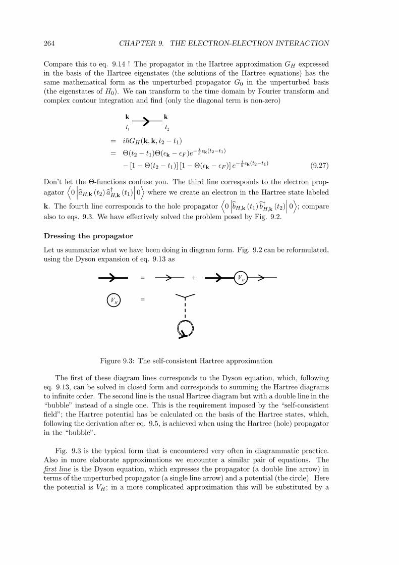
264 CHAPTER 9. THE ELECTRON-ELECTRON INTERACTION
Compare this to eq. 9.14 ! The propagator in the Hartree approximation GH expressedin the basis of the Hartree eigenstates (the solutions of the Hartree equations) has thesame mathematical form as the unperturbed propagator G0 in the unperturbed basis(the eigenstates of H0). We can transform to the time domain by Fourier transform andcomplex contour integration and find (only the diagonal term is non-zero)
2t1tk k
= i~GH(k,k, t2 − t1)= Θ(t2 − t1)Θ(²k − ²F )e−
i~ ²k(t2−t1)
− [1−Θ(t2 − t1)] [1−Θ(²k − ²F )] e−i~ ²k(t2−t1) (9.27)
Don’t let the Θ-functions confuse you. The third line corresponds to the electron prop-
agatorD0¯baH,k (t2)ba†H,k (t1)¯ 0E where we create an electron in the Hartree state labeled
k. The fourth line corresponds to the hole propagatorD0¯bbH,k (t1)bb†H,k (t2)¯ 0E; compare
also to eqs. 9.3. We have effectively solved the problem posed by Fig. 9.2.
Dressing the propagator
Let us summarize what we have been doing in diagram form. Fig. 9.2 can be reformulated,using the Dyson expansion of eq. 9.13 as
HV= +
HV =
Figure 9.3: The self-consistent Hartree approximation
The first of these diagram lines corresponds to the Dyson equation, which, followingeq. 9.13, can be solved in closed form and corresponds to summing the Hartree diagramsto infinite order. The second line is the usual Hartree diagram but with a double line in the“bubble” instead of a single one. This is the requirement imposed by the “self-consistentfield”; the Hartree potential has be calculated on the basis of the Hartree states, which,following the derivation after eq. 9.5, is achieved when using the Hartree (hole) propagatorin the “bubble”.
Fig. 9.3 is the typical form that is encountered very often in diagrammatic practice.Also in more elaborate approximations we encounter a similar pair of equations. Thefirst line is the Dyson equation, which expresses the propagator (a double line arrow) interms of the unperturbed propagator (a single line arrow) and a potential (the circle). Herethe potential is VH ; in a more complicated approximation this will be substituted by a
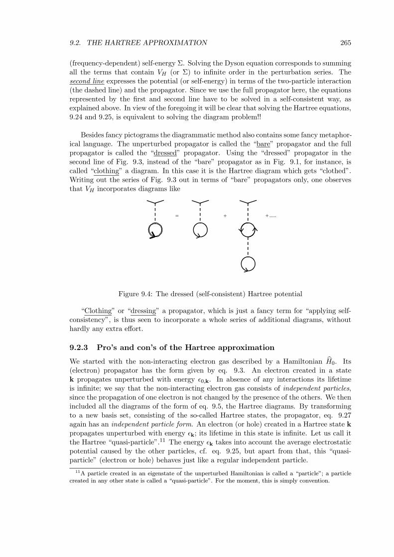
9.2. THE HARTREE APPROXIMATION 265
(frequency-dependent) self-energy Σ. Solving the Dyson equation corresponds to summingall the terms that contain VH (or Σ) to infinite order in the perturbation series. Thesecond line expresses the potential (or self-energy) in terms of the two-particle interaction(the dashed line) and the propagator. Since we use the full propagator here, the equationsrepresented by the first and second line have to be solved in a self-consistent way, asexplained above. In view of the foregoing it will be clear that solving the Hartree equations,9.24 and 9.25, is equivalent to solving the diagram problem!!
Besides fancy pictograms the diagrammatic method also contains some fancy metaphor-ical language. The unperturbed propagator is called the “bare” propagator and the fullpropagator is called the “dressed” propagator. Using the “dressed” propagator in thesecond line of Fig. 9.3, instead of the “bare” propagator as in Fig. 9.1, for instance, iscalled “clothing” a diagram. In this case it is the Hartree diagram which gets “clothed”.Writing out the series of Fig. 9.3 out in terms of “bare” propagators only, one observesthat VH incorporates diagrams like
= + .....+
Figure 9.4: The dressed (self-consistent) Hartree potential
“Clothing” or “dressing” a propagator, which is just a fancy term for “applying self-consistency”, is thus seen to incorporate a whole series of additional diagrams, withouthardly any extra effort.
9.2.3 Pro’s and con’s of the Hartree approximation
We started with the non-interacting electron gas described by a Hamiltonian bH0. Its(electron) propagator has the form given by eq. 9.3. An electron created in a statek propagates unperturbed with energy ²0,k. In absence of any interactions its lifetimeis infinite; we say that the non-interacting electron gas consists of independent particles,since the propagation of one electron is not changed by the presence of the others. We thenincluded all the diagrams of the form of eq. 9.5, the Hartree diagrams. By transformingto a new basis set, consisting of the so-called Hartree states, the propagator, eq. 9.27again has an independent particle form. An electron (or hole) created in a Hartree state kpropagates unperturbed with energy ²k; its lifetime in this state is infinite. Let us call itthe Hartree “quasi-particle”.11 The energy ²k takes into account the average electrostaticpotential caused by the other particles, cf. eq. 9.25, but apart from that, this “quasi-particle” (electron or hole) behaves just like a regular independent particle.
11A particle created in an eigenstate of the unperturbed Hamiltonian is called a “particle”; a particlecreated in any other state is called a “quasi-particle”. For the moment, this is simply convention.
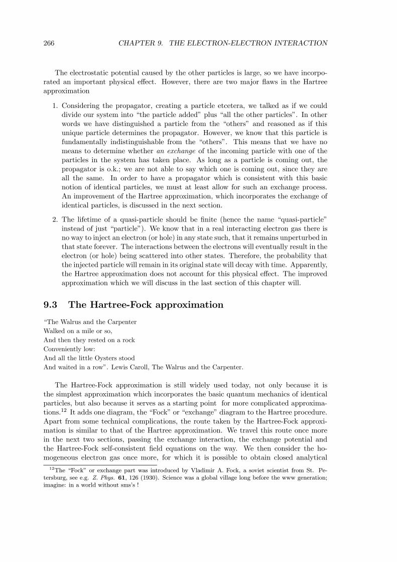
266 CHAPTER 9. THE ELECTRON-ELECTRON INTERACTION
The electrostatic potential caused by the other particles is large, so we have incorpo-rated an important physical effect. However, there are two major flaws in the Hartreeapproximation
1. Considering the propagator, creating a particle etcetera, we talked as if we coulddivide our system into “the particle added” plus “all the other particles”. In otherwords we have distinguished a particle from the “others” and reasoned as if thisunique particle determines the propagator. However, we know that this particle isfundamentally indistinguishable from the “others”. This means that we have nomeans to determine whether an exchange of the incoming particle with one of theparticles in the system has taken place. As long as a particle is coming out, thepropagator is o.k.; we are not able to say which one is coming out, since they areall the same. In order to have a propagator which is consistent with this basicnotion of identical particles, we must at least allow for such an exchange process.An improvement of the Hartree approximation, which incorporates the exchange ofidentical particles, is discussed in the next section.
2. The lifetime of a quasi-particle should be finite (hence the name “quasi-particle”instead of just “particle”). We know that in a real interacting electron gas there isno way to inject an electron (or hole) in any state such, that it remains unperturbed inthat state forever. The interactions between the electrons will eventually result in theelectron (or hole) being scattered into other states. Therefore, the probability thatthe injected particle will remain in its original state will decay with time. Apparently,the Hartree approximation does not account for this physical effect. The improvedapproximation which we will discuss in the last section of this chapter will.
9.3 The Hartree-Fock approximation
“The Walrus and the Carpenter
Walked on a mile or so,
And then they rested on a rock
Conveniently low:
And all the little Oysters stood
And waited in a row”. Lewis Caroll, The Walrus and the Carpenter.
The Hartree-Fock approximation is still widely used today, not only because it isthe simplest approximation which incorporates the basic quantum mechanics of identicalparticles, but also because it serves as a starting point for more complicated approxima-tions.12 It adds one diagram, the “Fock” or “exchange” diagram to the Hartree procedure.Apart from some technical complications, the route taken by the Hartree-Fock approxi-mation is similar to that of the Hartree approximation. We travel this route once morein the next two sections, passing the exchange interaction, the exchange potential andthe Hartree-Fock self-consistent field equations on the way. We then consider the ho-mogeneous electron gas once more, for which it is possible to obtain closed analytical
12The “Fock” or exchange part was introduced by Vladimir A. Fock, a soviet scientist from St. Pe-tersburg, see e.g. Z. Phys. 61, 126 (1930). Science was a global village long before the www generation;imagine: in a world without sms’s !
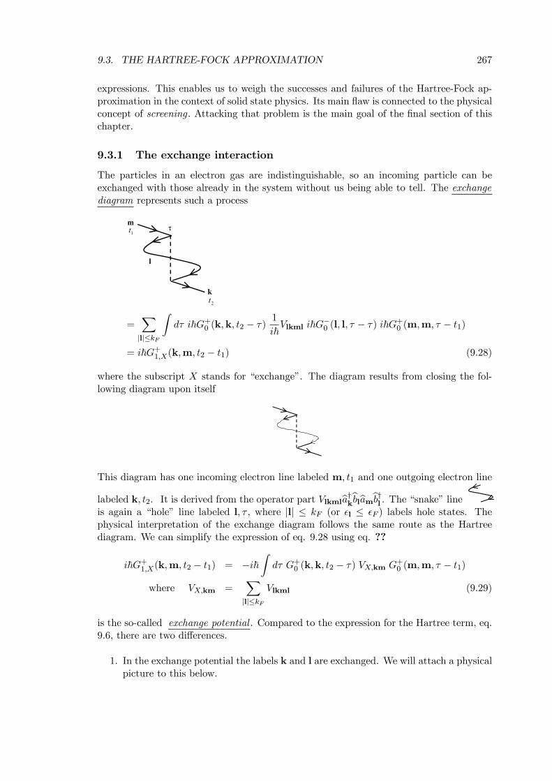
9.3. THE HARTREE-FOCK APPROXIMATION 267
expressions. This enables us to weigh the successes and failures of the Hartree-Fock ap-proximation in the context of solid state physics. Its main flaw is connected to the physicalconcept of screening . Attacking that problem is the main goal of the final section of thischapter.
9.3.1 The exchange interaction
The particles in an electron gas are indistinguishable, so an incoming particle can beexchanged with those already in the system without us being able to tell. The exchangediagram represents such a process
l
k
m1t
2t
τ
=X|l|≤kF
Zdτ i~G+0 (k,k, t2 − τ)
1
i~Vlkml i~G−0 (l, l, τ − τ) i~G+0 (m,m, τ − t1)
= i~G+1,X(k,m, t2 − t1) (9.28)
where the subscript X stands for “exchange”. The diagram results from closing the fol-lowing diagram upon itself
This diagram has one incoming electron line labeled m, t1 and one outgoing electron line
labeled k, t2. It is derived from the operator part Vlkmlba†kbblbambb†l . The “snake” lineis again a “hole” line labeled l, τ , where |l| ≤ kF (or ²l ≤ ²F ) labels hole states. Thephysical interpretation of the exchange diagram follows the same route as the Hartreediagram. We can simplify the expression of eq. 9.28 using eq. ??
i~G+1,X(k,m, t2 − t1) = −i~Zdτ G+0 (k,k, t2 − τ) VX,km G
+0 (m,m, τ − t1)
where VX,km =X|l|≤kF
Vlkml (9.29)
is the so-called exchange potential . Compared to the expression for the Hartree term, eq.9.6, there are two differences.
1. In the exchange potential the labels k and l are exchanged. We will attach a physicalpicture to this below.
268 CHAPTER 9. THE ELECTRON-ELECTRON INTERACTION
2. There is an overall “−” in front of the expression. There is no “bubble” sign rule inthis case; see the discussion around eq. 9.6.
Apart from these differences, the expression has the familiar first order perturbationform again, which means we can represent the exchange diagram as a potential scatteringdiagram.
l
k
m1t
2t
τ
= XVm
1tk
2t
Figure 9.5: The exchange potential
The exchange potential acts like a one particle potential, which scatters an incomingparticle in state m out into a state k. At time t = τ a hole is created in a state l whichis immediately filled again. To get a physical interpretation of the exchange potential, weuse the position representation once more
VX,km =X|l|≤kF
Vlkml
=X|l|≤kF
Z Zd3r1 d
3r2 φ∗l (r1)φ
∗k(r2)
e2
|r1 − r2|φm(r1)φl(r2)
=
Z Zd3r1 d
3r2 φ∗k(r2)VX(r2, r1)φm(r1) (9.30)
where the exchange potential in the position representation VX(r2, r1) is defined as
VX(r2, r1) = e2X|l|≤kF
φl(r2)φ∗l (r1)
|r1 − r2| (9.31)
Non-local exchange potential
This seemingly strange “potential” depends upon two arguments r1 and r2. The physicalinterpretation is as follows; |l| ≤ kF labels the one particle states which are occupied inthe ground state of the electron gas. At position r1 an incoming electron arrives in statem at time t = τ . At the same an electron-hole pair is created at position r2. The hole instate l proceeds to r1 where it recombines with the incoming electron, the created electroncomes out in state k. A shorter way of saying the same thing is: an electron comes inat r1 in state m and knocks out an electron at r2 in state k. This process is determinedby the “potential” VX(r2, r1) and proceeds via an intermediate hole. We need to extendour notion of the term “potential”. A normal potential would depend on a single positionin space r1; from now on we will call this a local potential. VX(r2, r1) depends on twopositions; it connects two arbitrary points in space; this we will call a non-local potential .
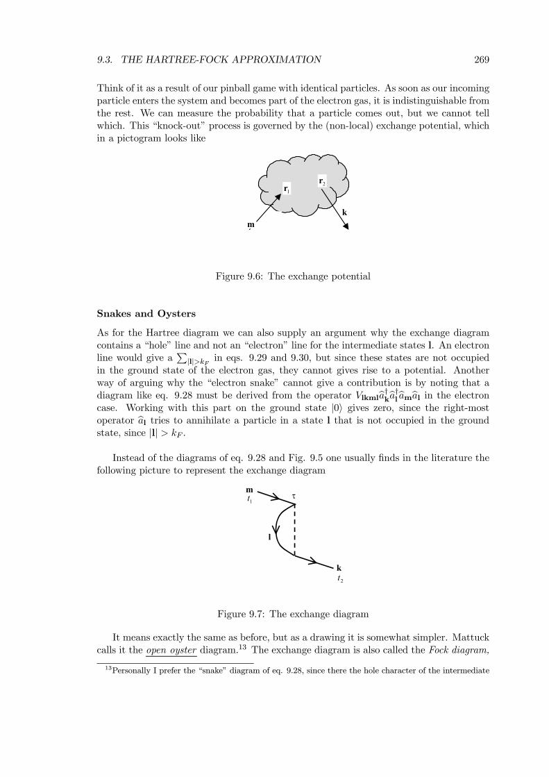
9.3. THE HARTREE-FOCK APPROXIMATION 269
Think of it as a result of our pinball game with identical particles. As soon as our incomingparticle enters the system and becomes part of the electron gas, it is indistinguishable fromthe rest. We can measure the probability that a particle comes out, but we cannot tellwhich. This “knock-out” process is governed by the (non-local) exchange potential, whichin a pictogram looks like
mk
1r2r
Figure 9.6: The exchange potential
Snakes and Oysters
As for the Hartree diagram we can also supply an argument why the exchange diagramcontains a “hole” line and not an “electron” line for the intermediate states l. An electronline would give a
P|l|>kF in eqs. 9.29 and 9.30, but since these states are not occupied
in the ground state of the electron gas, they cannot gives rise to a potential. Anotherway of arguing why the “electron snake” cannot give a contribution is by noting that adiagram like eq. 9.28 must be derived from the operator Vlkmlba†kba†lbambal in the electroncase. Working with this part on the ground state |0i gives zero, since the right-mostoperator bal tries to annihilate a particle in a state l that is not occupied in the groundstate, since |l| > kF .
Instead of the diagrams of eq. 9.28 and Fig. 9.5 one usually finds in the literature thefollowing picture to represent the exchange diagram
l
k
m1t
2t
τ
Figure 9.7: The exchange diagram
It means exactly the same as before, but as a drawing it is somewhat simpler. Mattuckcalls it the open oyster diagram.13 The exchange diagram is also called the Fock diagram,
13Personally I prefer the “snake” diagram of eq. 9.28, since there the hole character of the intermediate
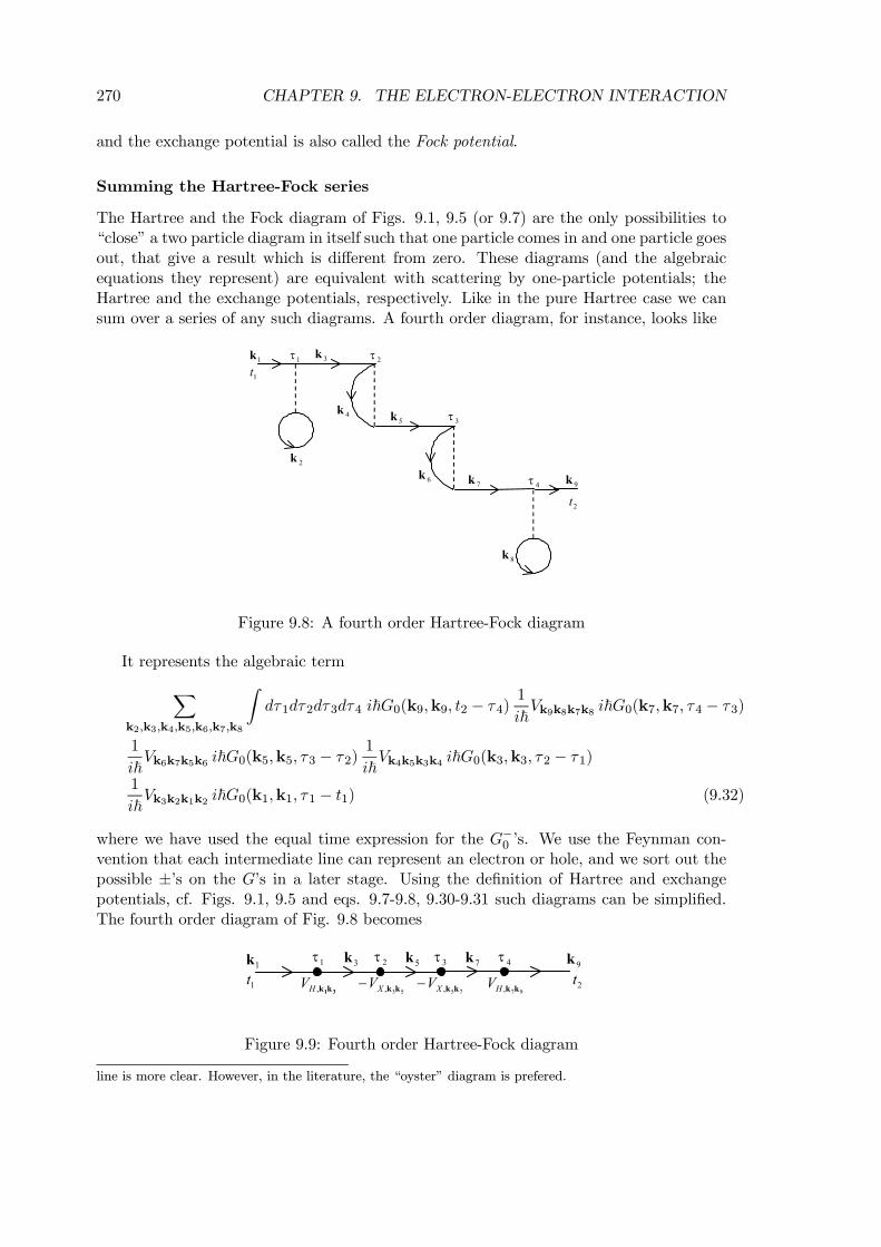
270 CHAPTER 9. THE ELECTRON-ELECTRON INTERACTION
and the exchange potential is also called the Fock potential.
Summing the Hartree-Fock series
The Hartree and the Fock diagram of Figs. 9.1, 9.5 (or 9.7) are the only possibilities to“close” a two particle diagram in itself such that one particle comes in and one particle goesout, that give a result which is different from zero. These diagrams (and the algebraicequations they represent) are equivalent with scattering by one-particle potentials; theHartree and the exchange potentials, respectively. Like in the pure Hartree case we cansum over a series of any such diagrams. A fourth order diagram, for instance, looks like
1τ1k1t
2t
2k
2τ
3τ
4τ
3k
4k5k
6k7k
8k
9k
Figure 9.8: A fourth order Hartree-Fock diagram
It represents the algebraic termXk2,k3,k4,k5,k6,k7,k8
Zdτ1dτ2dτ3dτ4 i~G0(k9,k9, t2 − τ4)
1
i~Vk9k8k7k8 i~G0(k7,k7, τ4 − τ3)
1
i~Vk6k7k5k6 i~G0(k5,k5, τ3 − τ2)
1
i~Vk4k5k3k4 i~G0(k3,k3, τ2 − τ1)
1
i~Vk3k2k1k2 i~G0(k1,k1, τ1 − t1) (9.32)
where we have used the equal time expression for the G−0 ’s. We use the Feynman con-vention that each intermediate line can represent an electron or hole, and we sort out thepossible ±’s on the G’s in a later stage. Using the definition of Hartree and exchangepotentials, cf. Figs. 9.1, 9.5 and eqs. 9.7-9.8, 9.30-9.31 such diagrams can be simplified.The fourth order diagram of Fig. 9.8 becomes
31kk,HV
53, kkXV− 75, kkXV− 97, kkHV1τ 2τ 3τ 4τ1k
1t 2t9k3k 5k 7k
Figure 9.9: Fourth order Hartree-Fock diagram
line is more clear. However, in the literature, the “oyster” diagram is prefered.
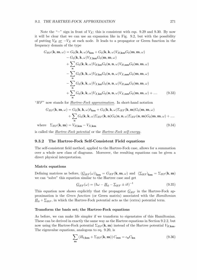
9.3. THE HARTREE-FOCK APPROXIMATION 271
Note the “−” sign in front of VX ; this is consistent with eqs. 9.29 and 9.30. By nowit will be clear that we can use an expansion like in Fig. 9.2, but with the possibilityof putting VH or −VX at each node. It leads to a propagator or Green function in thefrequency domain of the type
GHF (k,m,ω) = G0(k,k,ω)δkm +G0(k,k,ω)VH,kmG0(m,m,ω)
−G0(k,k,ω)VX,kmG0(m,m,ω)+Xn
G0(k,k,ω)VH,knG0(n,n,ω)VH,nmG0(m,m,ω)
−Xn
G0(k,k,ω)VH,knG0(n,n,ω)VX,nmG0(m,m,ω)
−Xn
G0(k,k,ω)VX,knG0(n,n,ω)VH,nmG0(m,m,ω)
+Xn
G0(k,k,ω)VX,knG0(n,n,ω)VX,nmG0(m,m,ω) + .... (9.33)
“HF” now stands for Hartree-Fock approximation. In short-hand notation
GHF (k,m,ω) = G0(k,k,ω)δkm +G0(k,k,ω)ΣHF (k,m)G0(m,m,ω)
+Xn
G0(k,k,ω)ΣHF (k,n)G0(n,n,ω)ΣHF (n,m)G0(m,m,ω) + ....
where ΣHF (k,m) = VH,km − VX,km (9.34)
is called the Hartree-Fock potential or the Hartree-Fock self-energy .
9.3.2 The Hartree-Fock Self-Consistent Field equations
The self-consistent field method, applied to the Hartree-Fock case, allows for a summationover a whole new class of diagrams. Moreover, the resulting equations can be given adirect physical interpretation.
Matrix equations
Defining matrices as before, (GHF (ω))km = GHF (k,m,ω) and (ΣHF )km = ΣHF (k,m)we can “solve” this equation similar to the Hartree case and get
GHF (ω) = (~ω −H0 − ΣHF ± iδ)−1 (9.35)
This equation now shows explicitly that the propagator GHF in the Hartree-Fock ap-proximation is the Green function (or Green matrix) associated with the HamiltonianH0 +ΣHF , in which the Hartree-Fock potential acts as the (extra) potential term.
Transform the basis set; the Hartree-Fock equations
As before, we can make life simpler if we transform to eigenstates of this Hamiltonian.These can be derived in exactly the same way as the Hartree equations in Section 9.2.2, butnow using the Hartree-Fock potential ΣHF (k,m) instead of the Hartree potential VH,km.The eigenvalue equations, analogous to eq. 9.20, isX
m
(H0,km +ΣHF (k,m))Cmn = ²nCkn (9.36)
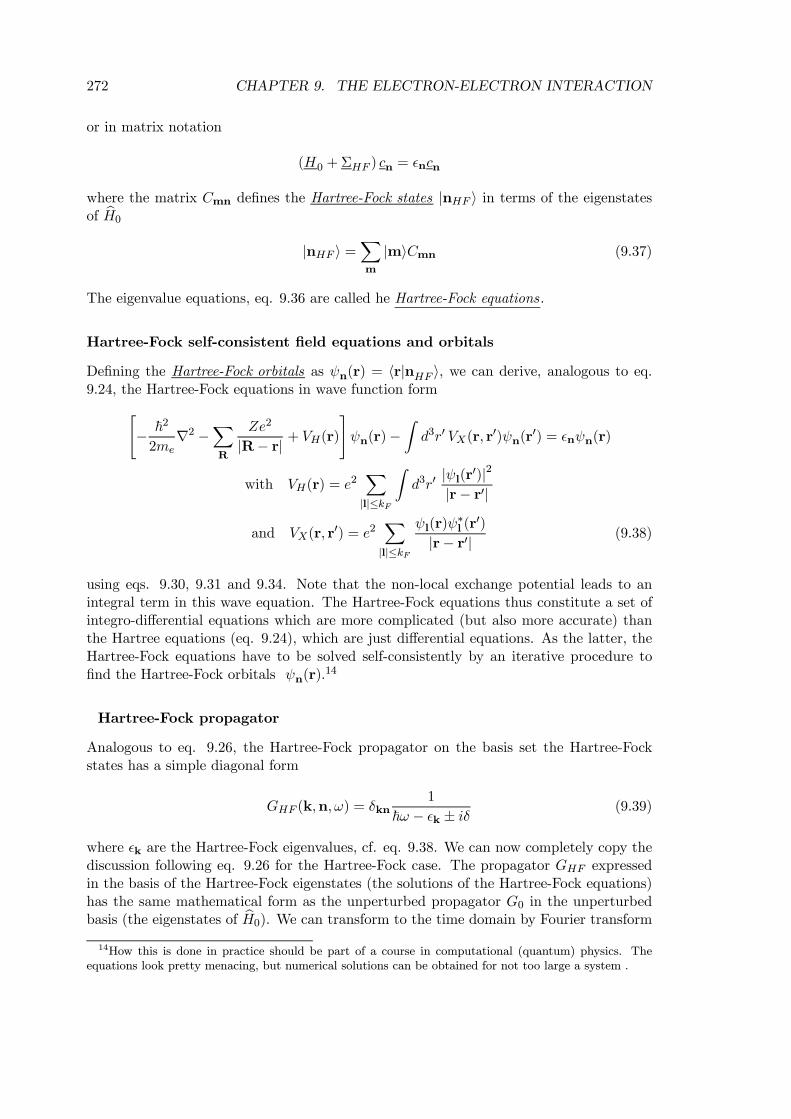
272 CHAPTER 9. THE ELECTRON-ELECTRON INTERACTION
or in matrix notation
(H0 +ΣHF ) cn = ²ncn
where the matrix Cmn defines the Hartree-Fock states |nHF i in terms of the eigenstatesof bH0
|nHF i =Xm
|miCmn (9.37)
The eigenvalue equations, eq. 9.36 are called he Hartree-Fock equations.
Hartree-Fock self-consistent field equations and orbitals
Defining the Hartree-Fock orbitals as ψn(r) = hr|nHF i, we can derive, analogous to eq.9.24, the Hartree-Fock equations in wave function form"
− ~2
2me∇2 −
XR
Ze2
|R− r| + VH(r)#ψn(r)−
Zd3r0 VX(r, r0)ψn(r
0) = ²nψn(r)
with VH(r) = e2X|l|≤kF
Zd3r0
|ψl(r0)|2|r− r0|
and VX(r, r0) = e2
X|l|≤kF
ψl(r)ψ∗l (r
0)|r− r0| (9.38)
using eqs. 9.30, 9.31 and 9.34. Note that the non-local exchange potential leads to anintegral term in this wave equation. The Hartree-Fock equations thus constitute a set ofintegro-differential equations which are more complicated (but also more accurate) thanthe Hartree equations (eq. 9.24), which are just differential equations. As the latter, theHartree-Fock equations have to be solved self-consistently by an iterative procedure tofind the Hartree-Fock orbitals ψn(r).
14
Hartree-Fock propagator
Analogous to eq. 9.26, the Hartree-Fock propagator on the basis set the Hartree-Fockstates has a simple diagonal form
GHF (k,n,ω) = δkn1
~ω − ²k ± iδ (9.39)
where ²k are the Hartree-Fock eigenvalues, cf. eq. 9.38. We can now completely copy thediscussion following eq. 9.26 for the Hartree-Fock case. The propagator GHF expressedin the basis of the Hartree-Fock eigenstates (the solutions of the Hartree-Fock equations)has the same mathematical form as the unperturbed propagator G0 in the unperturbedbasis (the eigenstates of bH0). We can transform to the time domain by Fourier transform
14How this is done in practice should be part of a course in computational (quantum) physics. Theequations look pretty menacing, but numerical solutions can be obtained for not too large a system .
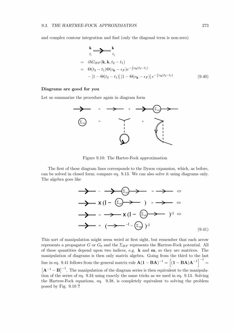
9.3. THE HARTREE-FOCK APPROXIMATION 273
and complex contour integration and find (only the diagonal term is non-zero)
2t1tk k
= i~GHF (k,k, t2 − t1)= Θ(t2 − t1)Θ(²k − ²F )e−
i~ ²k(t2−t1)
− [1−Θ(t2 − t1)] [1−Θ(²k − ²F )] e−i~ ²k(t2−t1) (9.40)
Diagrams are good for you
Let us summarize the procedure again in diagram form
HFΣ= +
=HFΣ +
Figure 9.10: The Hartee-Fock approximation
The first of these diagram lines corresponds to the Dyson expansion, which, as before,can be solved in closed form; compare eq. 9.13. We can also solve it using diagrams only.The algebra goes like
= ⇔− HFΣ
x (I − HFΣ ) = ⇔
= x (I − HFΣ )-1 ⇔
= ( HFΣ-1 − )-1(9.41)
This sort of manipulation might seem weird at first sight, but remember that each arrowrepresents a propagator G or G0 and the ΣHF represents the Hartree-Fock potential. Allof these quantities depend upon two indices, e.g. k and m, so they are matrices. Themanipulation of diagrams is then only matrix algebra. Going from the third to the last
line in eq. 9.41 follows from the general matrix rule A(1−BA)−1 =h(1−BA)A−1
i−1=£
A−1 −B¤−1. The manipulation of the diagram series is then equivalent to the manipula-tion of the series of eq. 9.34 using exactly the same tricks as we used in eq. 9.13. Solvingthe Hartree-Fock equations, eq. 9.38, is completely equivalent to solving the problemposed by Fig. 9.10 !!
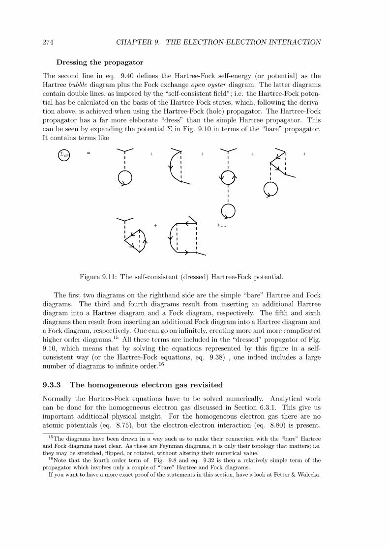
274 CHAPTER 9. THE ELECTRON-ELECTRON INTERACTION
Dressing the propagator
The second line in eq. 9.40 defines the Hartree-Fock self-energy (or potential) as theHartree bubble diagram plus the Fock exchange open oyster diagram. The latter diagramscontain double lines, as imposed by the “self-consistent field”; i.e. the Hartree-Fock poten-tial has be calculated on the basis of the Hartree-Fock states, which, following the deriva-tion above, is achieved when using the Hartree-Fock (hole) propagator. The Hartree-Fockpropagator has a far more eleborate “dress” than the simple Hartree propagator. Thiscan be seen by expanding the potential Σ in Fig. 9.10 in terms of the “bare” propagator.It contains terms like
=HFΣ + + + +
+ .....+
Figure 9.11: The self-consistent (dressed) Hartree-Fock potential.
The first two diagrams on the righthand side are the simple “bare” Hartree and Fockdiagrams. The third and fourth diagrams result from inserting an additional Hartreediagram into a Hartree diagram and a Fock diagram, respectively. The fifth and sixthdiagrams then result from inserting an additional Fock diagram into a Hartree diagram anda Fock diagram, respectively. One can go on infinitely, creating more and more complicatedhigher order diagrams.15 All these terms are included in the “dressed” propagator of Fig.9.10, which means that by solving the equations represented by this figure in a self-consistent way (or the Hartree-Fock equations, eq. 9.38) , one indeed includes a largenumber of diagrams to infinite order.16
9.3.3 The homogeneous electron gas revisited
Normally the Hartree-Fock equations have to be solved numerically. Analytical workcan be done for the homogeneous electron gas discussed in Section 6.3.1. This give usimportant additional physical insight. For the homogeneous electron gas there are noatomic potentials (eq. 8.75), but the electron-electron interaction (eq. 8.80) is present.
15The diagrams have been drawn in a way such as to make their connection with the “bare” Hartreeand Fock diagrams most clear. As these are Feynman diagrams, it is only their topology that matters; i.e.they may be stretched, flipped, or rotated, without altering their numerical value.16Note that the fourth order term of Fig. 9.8 and eq. 9.32 is then a relatively simple term of the
propagator which involves only a couple of “bare” Hartree and Fock diagrams.If you want to have a more exact proof of the statements in this section, have a look at Fetter & Walecka.
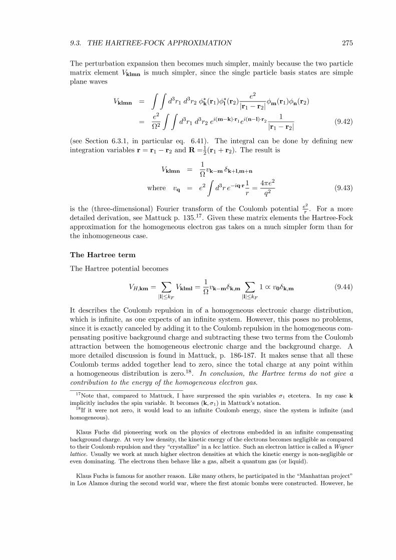
9.3. THE HARTREE-FOCK APPROXIMATION 275
The perturbation expansion then becomes much simpler, mainly because the two particlematrix element Vklmn is much simpler, since the single particle basis states are simpleplane waves
Vklmn =
Z Zd3r1 d
3r2 φ∗k(r1)φ
∗l (r2)
e2
|r1 − r2|φm(r1)φn(r2)
=e2
Ω2
Z Zd3r1 d
3r2 ei(m−k)·r1ei(n−l)·r2
1
|r1 − r2| (9.42)
(see Section 6.3.1, in particular eq. 6.41). The integral can be done by defining newintegration variables r = r1 − r2 and R =1
2(r1 + r2). The result is
Vklmn =1
Ωvk−m δk+l,m+n
where vq = e2Zd3r e−iq·r
1
r=4πe2
q2(9.43)
is the (three-dimensional) Fourier transform of the Coulomb potential e2
r . For a moredetailed derivation, see Mattuck p. 135.17. Given these matrix elements the Hartree-Fockapproximation for the homogeneous electron gas takes on a much simpler form than forthe inhomogeneous case.
The Hartree term
The Hartree potential becomes
VH,km =X|l|≤kF
Vklml =1
Ωvk−mδk,m
X|l|≤kF
1 ∝ v0δk,m (9.44)
It describes the Coulomb repulsion in of a homogeneous electronic charge distribution,which is infinite, as one expects of an infinite system. However, this poses no problems,since it is exactly canceled by adding it to the Coulomb repulsion in the homogeneous com-pensating positive background charge and subtracting these two terms from the Coulombattraction between the homogeneous electronic charge and the background charge. Amore detailed discussion is found in Mattuck, p. 186-187. It makes sense that all theseCoulomb terms added together lead to zero, since the total charge at any point withina homogeneous distribution is zero.18. In conclusion, the Hartree terms do not give acontribution to the energy of the homogeneous electron gas.
17Note that, compared to Mattuck, I have surpressed the spin variables σ1 etcetera. In my case kimplicitly includes the spin variable. It becomes (k,σ1) in Mattuck’s notation.18If it were not zero, it would lead to an infinite Coulomb energy, since the system is infinite (and
homogeneous).
Klaus Fuchs did pioneering work on the physics of electrons embedded in an infinite compensatingbackground charge. At very low density, the kinetic energy of the electrons becomes negligible as comparedto their Coulomb repulsion and they “crystallize” in a bcc lattice. Such an electron lattice is called aWignerlattice. Usually we work at much higher electron densities at which the kinetic energy is non-negligible oreven dominating. The electrons then behave like a gas, albeit a quantum gas (or liquid).
Klaus Fuchs is famous for another reason. Like many others, he participated in the “Manhattan project”in Los Alamos during the second world war, where the first atomic bombs were constructed. However, he
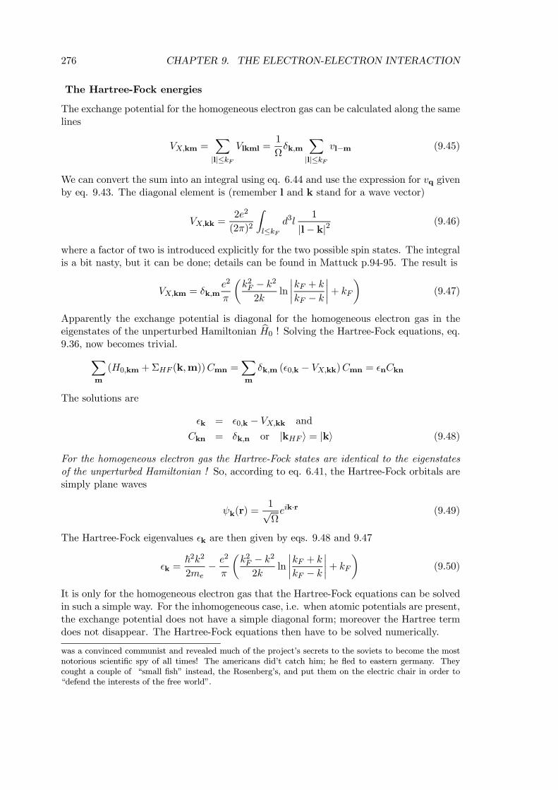
276 CHAPTER 9. THE ELECTRON-ELECTRON INTERACTION
The Hartree-Fock energies
The exchange potential for the homogeneous electron gas can be calculated along the samelines
VX,km =X|l|≤kF
Vlkml =1
Ωδk,m
X|l|≤kF
vl−m (9.45)
We can convert the sum into an integral using eq. 6.44 and use the expression for vq givenby eq. 9.43. The diagonal element is (remember l and k stand for a wave vector)
VX,kk =2e2
(2π)2
Zl≤kF
d3l1
|l− k|2 (9.46)
where a factor of two is introduced explicitly for the two possible spin states. The integralis a bit nasty, but it can be done; details can be found in Mattuck p.94-95. The result is
VX,km = δk,me2
π
µk2F − k22k
ln
¯kF + k
kF − k¯+ kF
¶(9.47)
Apparently the exchange potential is diagonal for the homogeneous electron gas in theeigenstates of the unperturbed Hamiltonian bH0 ! Solving the Hartree-Fock equations, eq.9.36, now becomes trivial.X
m
(H0,km +ΣHF (k,m))Cmn =Xm
δk,m (²0,k − VX,kk)Cmn = ²nCkn
The solutions are
²k = ²0,k − VX,kk and
Ckn = δk,n or |kHF i = |ki (9.48)
For the homogeneous electron gas the Hartree-Fock states are identical to the eigenstatesof the unperturbed Hamiltonian ! So, according to eq. 6.41, the Hartree-Fock orbitals aresimply plane waves
ψk(r) =1√Ωeik·r (9.49)
The Hartree-Fock eigenvalues ²k are then given by eqs. 9.48 and 9.47
²k =~2k2
2me− e
2
π
µk2F − k22k
ln
¯kF + k
kF − k¯+ kF
¶(9.50)
It is only for the homogeneous electron gas that the Hartree-Fock equations can be solvedin such a simple way. For the inhomogeneous case, i.e. when atomic potentials are present,the exchange potential does not have a simple diagonal form; moreover the Hartree termdoes not disappear. The Hartree-Fock equations then have to be solved numerically.
was a convinced communist and revealed much of the project’s secrets to the soviets to become the mostnotorious scientific spy of all times! The americans did’t catch him; he fled to eastern germany. Theycought a couple of “small fish” instead, the Rosenberg’s, and put them on the electric chair in order to“defend the interests of the free world”.
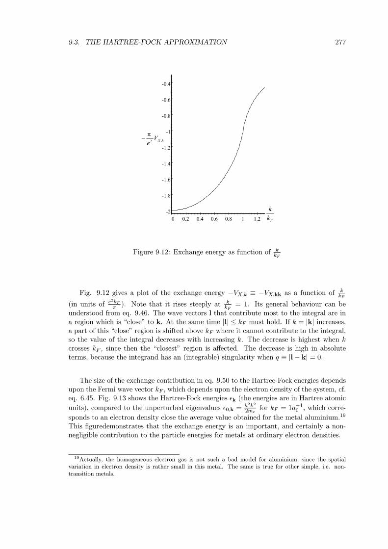
9.3. THE HARTREE-FOCK APPROXIMATION 277
-2
-1.8
-1.6
-1.4
-1.2
-1
-0.8
-0.6
-0.4
0 0.2 0.4 0.6 0.8 1 1.2k
Fkk
kXVe ,2
π−
Figure 9.12: Exchange energy as function of kkF
Fig. 9.12 gives a plot of the exchange energy −VX,k ≡ −VX,kk as a function of kkF
(in units of e2kFπ ). Note that it rises steeply at k
kF= 1. Its general behaviour can be
understood from eq. 9.46. The wave vectors l that contribute most to the integral are ina region which is “close” to k. At the same time |l| ≤ kF must hold. If k = |k| increases,a part of this “close” region is shifted above kF where it cannot contribute to the integral,so the value of the integral decreases with increasing k. The decrease is highest when kcrosses kF , since then the “closest” region is affected. The decrease is high in absoluteterms, because the integrand has an (integrable) singularity when q ≡ |l− k| = 0.
The size of the exchange contribution in eq. 9.50 to the Hartree-Fock energies dependsupon the Fermi wave vector kF , which depends upon the electron density of the system, cf.eq. 6.45. Fig. 9.13 shows the Hartree-Fock energies ²k (the energies are in Hartree atomic
units), compared to the unperturbed eigenvalues ²0,k =~2k22me
for kF = 1a−10 , which corre-
sponds to an electron density close the average value obtained for the metal aluminium.19
This figuredemonstrates that the exchange energy is an important, and certainly a non-negligible contribution to the particle energies for metals at ordinary electron densities.
19Actually, the homogeneous electron gas is not such a bad model for aluminium, since the spatialvariation in electron density is rather small in this metal. The same is true for other simple, i.e. non-transition metals.
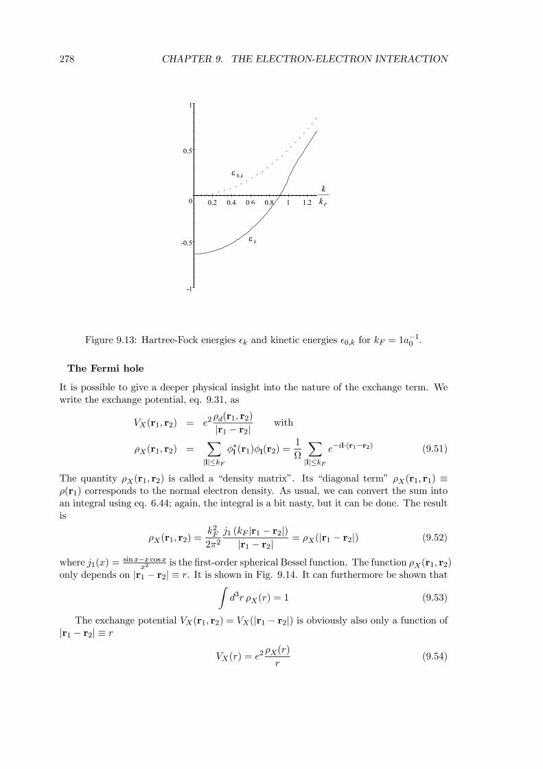
278 CHAPTER 9. THE ELECTRON-ELECTRON INTERACTION
-1
-0.5
0
0.5
1
0.2 0.4 0.6 0.8 1 1.2k Fk
k
kε
k,0ε
Figure 9.13: Hartree-Fock energies ²k and kinetic energies ²0,k for kF = 1a−10 .
The Fermi hole
It is possible to give a deeper physical insight into the nature of the exchange term. Wewrite the exchange potential, eq. 9.31, as
VX(r1, r2) = e2ρd(r1, r2)
|r1 − r2| with
ρX(r1, r2) =X|l|≤kF
φ∗l (r1)φl(r2) =1
Ω
X|l|≤kF
e−il·(r1−r2) (9.51)
The quantity ρX(r1, r2) is called a “density matrix”. Its “diagonal term” ρX(r1, r1) ≡ρ(r1) corresponds to the normal electron density. As usual, we can convert the sum intoan integral using eq. 6.44; again, the integral is a bit nasty, but it can be done. The resultis
ρX(r1, r2) =k2F2π2
j1 (kF |r1 − r2|)|r1 − r2| = ρX(|r1 − r2|) (9.52)
where j1(x) =sinx−x cosx
x2is the first-order spherical Bessel function. The function ρX(r1, r2)
only depends on |r1 − r2| ≡ r. It is shown in Fig. 9.14. It can furthermore be shown thatZd3r ρX(r) = 1 (9.53)
The exchange potential VX(r1, r2) = VX(|r1 − r2|) is obviously also only a function of|r1 − r2| ≡ r
VX(r) = e2ρX(r)
r(9.54)
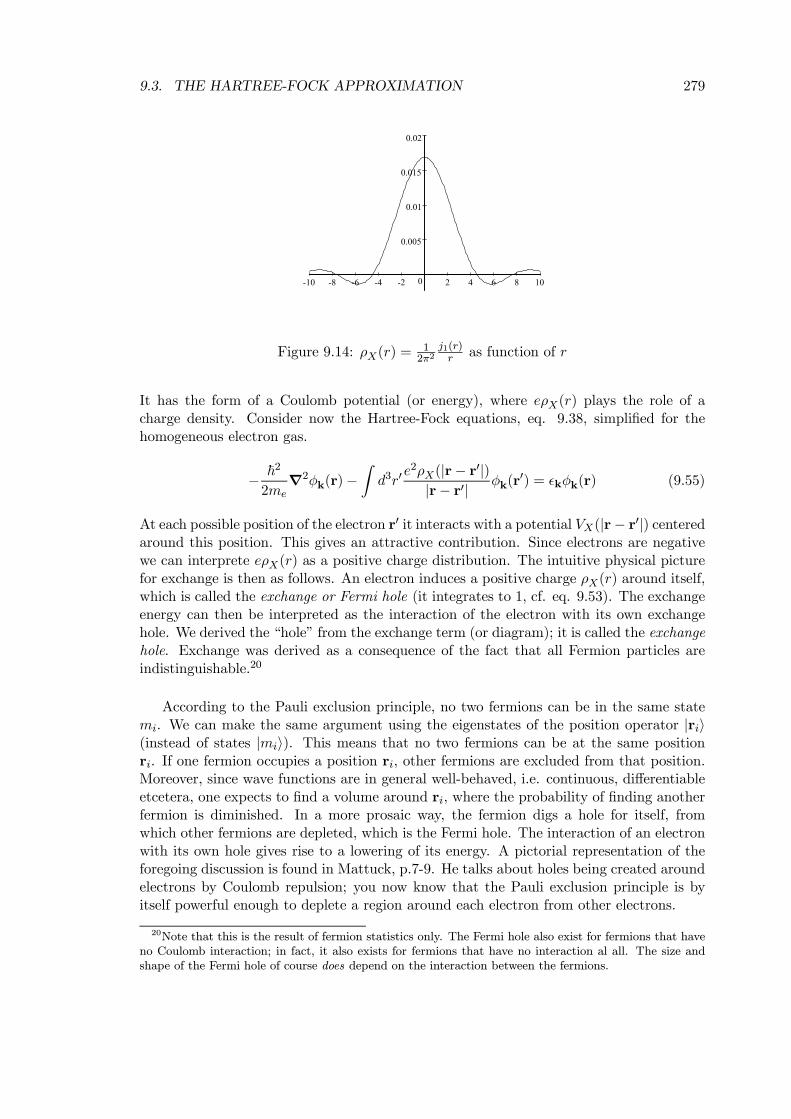
9.3. THE HARTREE-FOCK APPROXIMATION 279
0
0.005
0.01
0.015
0.02
-10 -8 -6 -4 -2 2 4 6 8 10
Figure 9.14: ρX(r) =12π2
j1(r)r as function of r
It has the form of a Coulomb potential (or energy), where eρX(r) plays the role of acharge density. Consider now the Hartree-Fock equations, eq. 9.38, simplified for thehomogeneous electron gas.
− ~2
2me∇2φk(r)−
Zd3r0
e2ρX(|r− r0|)|r− r0| φk(r
0) = ²kφk(r) (9.55)
At each possible position of the electron r0 it interacts with a potential VX(|r− r0|) centeredaround this position. This gives an attractive contribution. Since electrons are negativewe can interprete eρX(r) as a positive charge distribution. The intuitive physical picturefor exchange is then as follows. An electron induces a positive charge ρX(r) around itself,which is called the exchange or Fermi hole (it integrates to 1, cf. eq. 9.53). The exchangeenergy can then be interpreted as the interaction of the electron with its own exchangehole. We derived the “hole” from the exchange term (or diagram); it is called the exchangehole. Exchange was derived as a consequence of the fact that all Fermion particles areindistinguishable.20
According to the Pauli exclusion principle, no two fermions can be in the same statemi. We can make the same argument using the eigenstates of the position operator |rii(instead of states |mii). This means that no two fermions can be at the same positionri. If one fermion occupies a position ri, other fermions are excluded from that position.Moreover, since wave functions are in general well-behaved, i.e. continuous, differentiableetcetera, one expects to find a volume around ri, where the probability of finding anotherfermion is diminished. In a more prosaic way, the fermion digs a hole for itself, fromwhich other fermions are depleted, which is the Fermi hole. The interaction of an electronwith its own hole gives rise to a lowering of its energy. A pictorial representation of theforegoing discussion is found in Mattuck, p.7-9. He talks about holes being created aroundelectrons by Coulomb repulsion; you now know that the Pauli exclusion principle is byitself powerful enough to deplete a region around each electron from other electrons.
20Note that this is the result of fermion statistics only. The Fermi hole also exist for fermions that haveno Coulomb interaction; in fact, it also exists for fermions that have no interaction al all. The size andshape of the Fermi hole of course does depend on the interaction between the fermions.
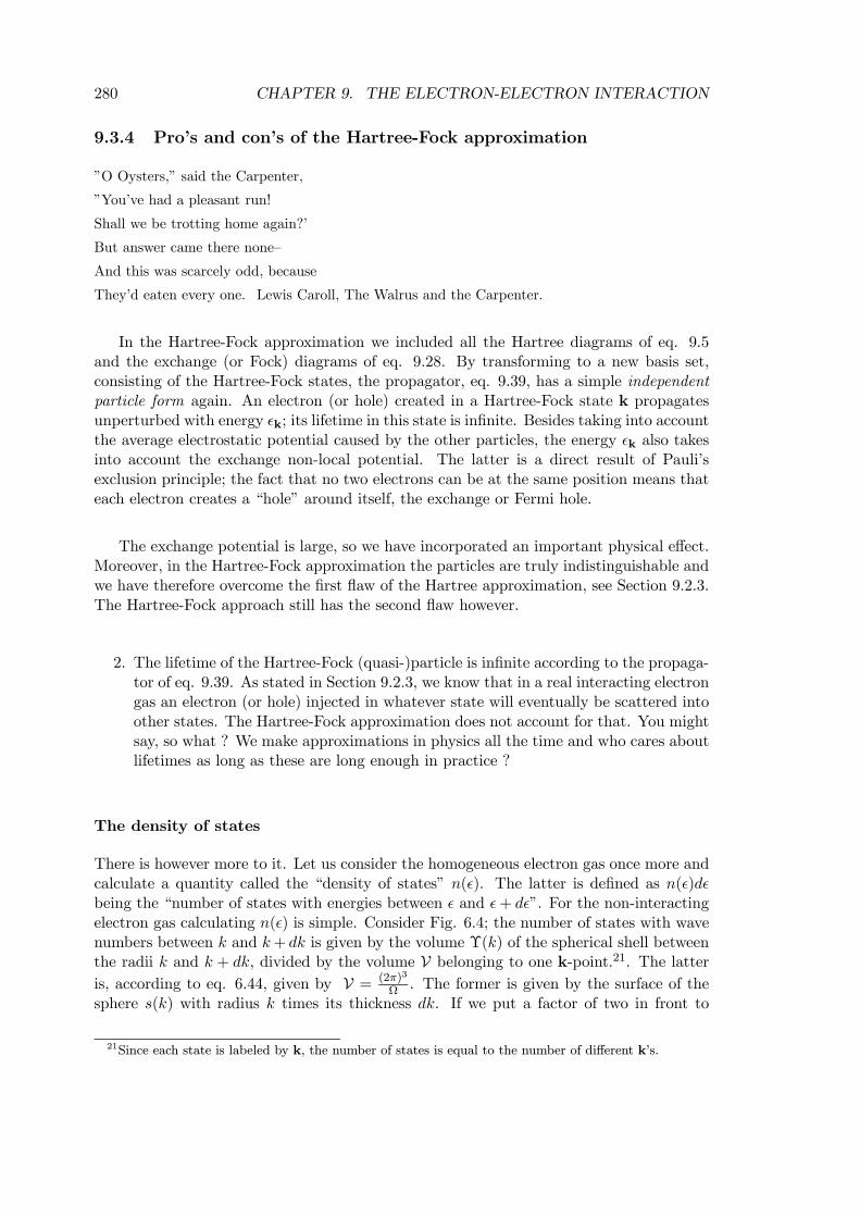
280 CHAPTER 9. THE ELECTRON-ELECTRON INTERACTION
9.3.4 Pro’s and con’s of the Hartree-Fock approximation
”O Oysters,” said the Carpenter,
”You’ve had a pleasant run!
Shall we be trotting home again?’
But answer came there none—
And this was scarcely odd, because
They’d eaten every one. Lewis Caroll, The Walrus and the Carpenter.
In the Hartree-Fock approximation we included all the Hartree diagrams of eq. 9.5and the exchange (or Fock) diagrams of eq. 9.28. By transforming to a new basis set,consisting of the Hartree-Fock states, the propagator, eq. 9.39, has a simple independentparticle form again. An electron (or hole) created in a Hartree-Fock state k propagatesunperturbed with energy ²k; its lifetime in this state is infinite. Besides taking into accountthe average electrostatic potential caused by the other particles, the energy ²k also takesinto account the exchange non-local potential. The latter is a direct result of Pauli’sexclusion principle; the fact that no two electrons can be at the same position means thateach electron creates a “hole” around itself, the exchange or Fermi hole.
The exchange potential is large, so we have incorporated an important physical effect.Moreover, in the Hartree-Fock approximation the particles are truly indistinguishable andwe have therefore overcome the first flaw of the Hartree approximation, see Section 9.2.3.The Hartree-Fock approach still has the second flaw however.
2. The lifetime of the Hartree-Fock (quasi-)particle is infinite according to the propaga-tor of eq. 9.39. As stated in Section 9.2.3, we know that in a real interacting electrongas an electron (or hole) injected in whatever state will eventually be scattered intoother states. The Hartree-Fock approximation does not account for that. You mightsay, so what ? We make approximations in physics all the time and who cares aboutlifetimes as long as these are long enough in practice ?
The density of states
There is however more to it. Let us consider the homogeneous electron gas once more andcalculate a quantity called the “density of states” n(²). The latter is defined as n(²)d²being the “number of states with energies between ² and ²+ d²”. For the non-interactingelectron gas calculating n(²) is simple. Consider Fig. 6.4; the number of states with wavenumbers between k and k+ dk is given by the volume Υ(k) of the spherical shell betweenthe radii k and k + dk, divided by the volume V belonging to one k-point.21. The latteris, according to eq. 6.44, given by V = (2π)3
Ω . The former is given by the surface of thesphere s(k) with radius k times its thickness dk. If we put a factor of two in front to
21Since each state is labeled by k, the number of states is equal to the number of different k’s.
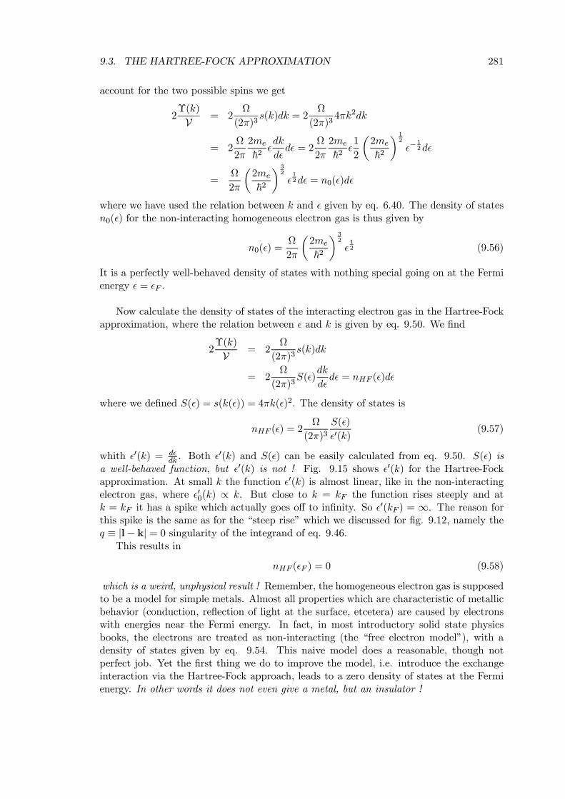
9.3. THE HARTREE-FOCK APPROXIMATION 281
account for the two possible spins we get
2Υ(k)
V = 2Ω
(2π)3s(k)dk = 2
Ω
(2π)34πk2dk
= 2Ω
2π
2me~2²dk
d²d² = 2
Ω
2π
2me
~2²1
2
µ2me
~2
¶12
²−12d²
=Ω
2π
µ2me
~2
¶ 32
²12d² = n0(²)d²
where we have used the relation between k and ² given by eq. 6.40. The density of statesn0(²) for the non-interacting homogeneous electron gas is thus given by
n0(²) =Ω
2π
µ2me~2
¶ 32
²12 (9.56)
It is a perfectly well-behaved density of states with nothing special going on at the Fermienergy ² = ²F .
Now calculate the density of states of the interacting electron gas in the Hartree-Fockapproximation, where the relation between ² and k is given by eq. 9.50. We find
2Υ(k)
V = 2Ω
(2π)3s(k)dk
= 2Ω
(2π)3S(²)
dk
d²d² = nHF (²)d²
where we defined S(²) = s(k(²)) = 4πk(²)2. The density of states is
nHF (²) = 2Ω
(2π)3S(²)
²0(k)(9.57)
whith ²0(k) = d²dk . Both ²
0(k) and S(²) can be easily calculated from eq. 9.50. S(²) isa well-behaved function, but ²0(k) is not ! Fig. 9.15 shows ²0(k) for the Hartree-Fockapproximation. At small k the function ²0(k) is almost linear, like in the non-interactingelectron gas, where ²00(k) ∝ k. But close to k = kF the function rises steeply and atk = kF it has a spike which actually goes off to infinity. So ²
0(kF ) = ∞. The reason forthis spike is the same as for the “steep rise” which we discussed for fig. 9.12, namely theq ≡ |l− k| = 0 singularity of the integrand of eq. 9.46.
This results in
nHF (²F ) = 0 (9.58)
which is a weird, unphysical result ! Remember, the homogeneous electron gas is supposedto be a model for simple metals. Almost all properties which are characteristic of metallicbehavior (conduction, reflection of light at the surface, etcetera) are caused by electronswith energies near the Fermi energy. In fact, in most introductory solid state physicsbooks, the electrons are treated as non-interacting (the “free electron model”), with adensity of states given by eq. 9.54. This naive model does a reasonable, though notperfect job. Yet the first thing we do to improve the model, i.e. introduce the exchangeinteraction via the Hartree-Fock approach, leads to a zero density of states at the Fermienergy. In other words it does not even give a metal, but an insulator !
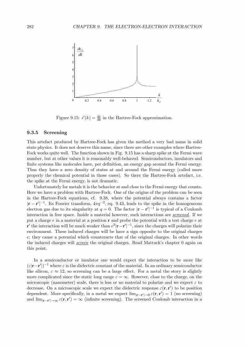
282 CHAPTER 9. THE ELECTRON-ELECTRON INTERACTION
0
1
2
3
4
5
6
7
0.2 0.4 0.6 0.8 1 1.2 Fkk
dkd kε
Figure 9.15: ²0(k) = d²dk in the Hartree-Fock approximation.
9.3.5 Screening
This artefact produced by Hartree-Fock has given the method a very bad name in solidstate physics. It does not deserve this name, since there are other examples where Hartree-Fock works quite well. The function shown in Fig. 9.15 has a sharp spike at the Fermi wavenumber, but at other values it is reasonably well-behaved. Semiconductors, insulators andfinite systems like molecules have, per definition, an energy gap around the Fermi energy.Thus they have a zero density of states at and around the Fermi energy (called moreproperly the chemical potential in those cases). So there the Hartree-Fock artefact, i.e.the spike at the Fermi energy, is not dramatic.
Unfortunately for metals it is the behavior at and close to the Fermi energy that counts.Here we have a problem with Hartree-Fock. One of the origins of the problem can be seenin the Hartree-Fock equations, cf. 9.38, where the potential always contains a factor|r− r0|−1. Its Fourier transform, 4πq−2, eq. 9.43, leads to the spike in the homogeneouselectron gas due to its singularity at q = 0. The factor |r− r0|−1 is typical of a Coulombinteraction in free space. Inside a material however, such interactions are screened . If weput a charge e in a material at a position r and probe the potential with a test charge e atr0 the interaction will be much weaker than e2|r−r0|−1, since the charges will polarize theirenvironment. These induced charges will be have a sign opposite to the original chargese; they cause a potential which counteracts that of the original charges. In other wordsthe induced charges will screen the original charges. Read Mattuck’s chapter 0 again onthis point.
In a semiconductor or insulator one would expect the interaction to be more like(ε|r−r0|)−1 where ε is the dielectric constant of the material. In an ordinary semiconductorlike silicon, ε ≈ 12, so screening can be a large effect. For a metal the story is slightlymore complicated since the static long range ε =∞. However, close to the charge, on themicroscopic (nanometer) scale, there is less or no material to polarize and we expect ε todecrease. On a microscopic scale we expect the dielectric response ε(r, r0) to be positiondependent. More specifically, in a metal we expect lim|r−r0|→0 ε(r, r0) = 1 (no screening)and lim|r−r0|→∞ ε(r, r0) = ∞ (infinite screening). The screened Coulomb interaction in a
9.4. THE RANDOM PHASE APPROXIMATION (RPA) 283
metal, which contains a ε(r, r0)−1 like factor, should therefore be confined to a region ofr0 that is close to r. In other words, the screened Coulomb interaction in a metal has afinite range. It leads to much weaker interaction between the electrons as discussed in thenext section. Mathematically spoken, it also gives a smooth Fourier transform, which doesnot have a singularity at q = 0. Therefore we expect screening to lift the Hartree-Fockartefact discussed above.
Moreover, in our propagator “experiment” (or quantum pinball game if you like) weare not dealing with static charges, but dynamic ones, since we are shooting an extraparticle into our system. The material must have time to respond, and its response tofast particles will in general be different from its response to slow ones. In other words,we expect a frequency dependent screening ε(r, r0,ω), also called the dielectric responsefunction, to play the central role. The slowness of response of the system to an incomingparticle eventually leads to scattering of the particle and thus a finite lifetime.22 Screeningis the subject of the next section.
9.4 The Random Phase Approximation (RPA)
“What’s in a name? That which we call a rose, by any other name would smell as sweet.”, William
Shakespeare, Romeo and Juliet.
As discussed in the previous section, to get rid of the artefacts produced by the Hartree-Fock approximation, which are due to the long range of the Coulomb interaction, one hasto introduce a dielectric screening of that interaction. Screening the long range part ofthe Coulomb interaction turns the strongly interacting electron gas into a gas of screenedelectrons which interact via a much weaker effective short-range potential. The screenedelectrons are quasi-particles; one expects that the screening charge that surrounds anelectron cannot follow the electron instantaneously. This leads to scattering and a finitelifetime of the electron.23 The simplest approximation that takes these physical effects intoaccount is called the random phase approximation or RPA. This approximation is namedafter the french-american couple Jean-Marie Random and An Y. Phase. No, just kidding,the reasons are purely historical; in the usual formulation there is not a phase in sight, letalone a random phase. The name unfortunately has been stuck in many particle physics,so we have no option but to use it.24 In this section we use the diagram approach tointroduce RPA. Application to the homogeneous electron gas illustrates that the physicaleffects discussed above are indeed included.
22Although this is a classical picture and thus not valid, one could say that the material can not giveway to a fast electron fast enough. The electron (and its Fermi hole) must be dragged through an electrongas which has a certain “viscosity” (although this is again not the right word, it is the slowness of dielectricresponse that counts). This gives rise to “losses”, or a decay of the probability of the electron to remainin its original state, which we describe by a finite lifetime. On a quantum level, these “losses” can bedescribed as scattering to other states.23or rather, of the state the electron occupies. The electron itsself of course does not dissappear; it is
scattered into other states.24The name RPA was invented by D. Bohm and D. Pines, see D. Pines, Elementary Excitations in
Solids, (Perseus, Reading, 1999). The diagrammatic approach was introduced by M Gell-Mann69 and K.A. Brueckner.
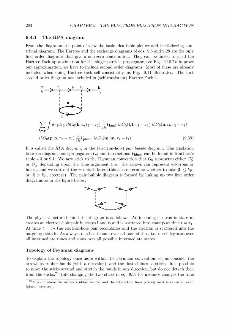
284 CHAPTER 9. THE ELECTRON-ELECTRON INTERACTION
9.4.1 The RPA diagram
From the diagrammatic point of view the basic idea is simple; we add the following non-trivial diagram. The Hartree and the exchange diagrams of eqs. 9.5 and 9.28 are the onlyfirst order diagrams that give a non-zero contribution. They can be linked to yield theHartree-Fock approximation for the single particle propagator, see Fig. 9.10.To improveour approximation, we have to include second order diagrams. Most of these are alreadyincluded when doing Hartree-Fock self-consistently, as Fig. 9.11 illustrates. The firstsecond order diagram not included in (self-consistent) Hartree-Fock is
m1t
k2t
l
n
p1τ 2τ
Xl,n,p
Zdτ1dτ2 i~G0(k,k, t2 − τ2)
1
i~Vknpl i~G0(l, l, τ2 − τ1) i~G0(n,n, τ2 − τ1)
i~G0(p,p, τ2 − τ1)1
i~Vplmn i~G0(m,m, τ1 − t1) (9.59)
It is called the RPA diagram, or the (electron-hole) pair bubble diagram. The trnslationbetween diagrams and propagators G0 and interactions Vklmn can be found in Mattuck’stable 4.3 or 9.1. We now stick to the Feynman convention that G0 represents either G
+0
or G−0 depending upon the time argument (i.e. the arrows can represent electrons orholes), and we sort out the ± details later (this also determine whether to take |l| ≤ kF ,or |l| > kF , etcetera). The pair bubble diagram is formed by linking up two first orderdiagrams as in the figure below.
The physical picture behind this diagram is as follows. An incoming electron in state mcreates an electron-hole pair in states l and n and is scattered into state p at time t = τ1.At time t = τ2 the electron-hole pair recombines and the electron is scattered into theoutgoing state k. As always, one has to sum over all possibilities, i.e. one integrates overall intermediate times and sums over all possible intermediate states.
Topology of Feynman diagrams
To explain the topology once more within the Feynman convention, let us consider thearrows as rubber bands (with a direction), and the dotted lines as sticks. It is possibleto move the sticks around and stretch the bands in any direction, but do not detach thenfrom the sticks.25 Interchanging the two sticks in eq. 9.59 for instance changes the time
25A point where the arrows (rubber bands) and the interaction lines (sticks) meet is called a vertex(plural: vertices).
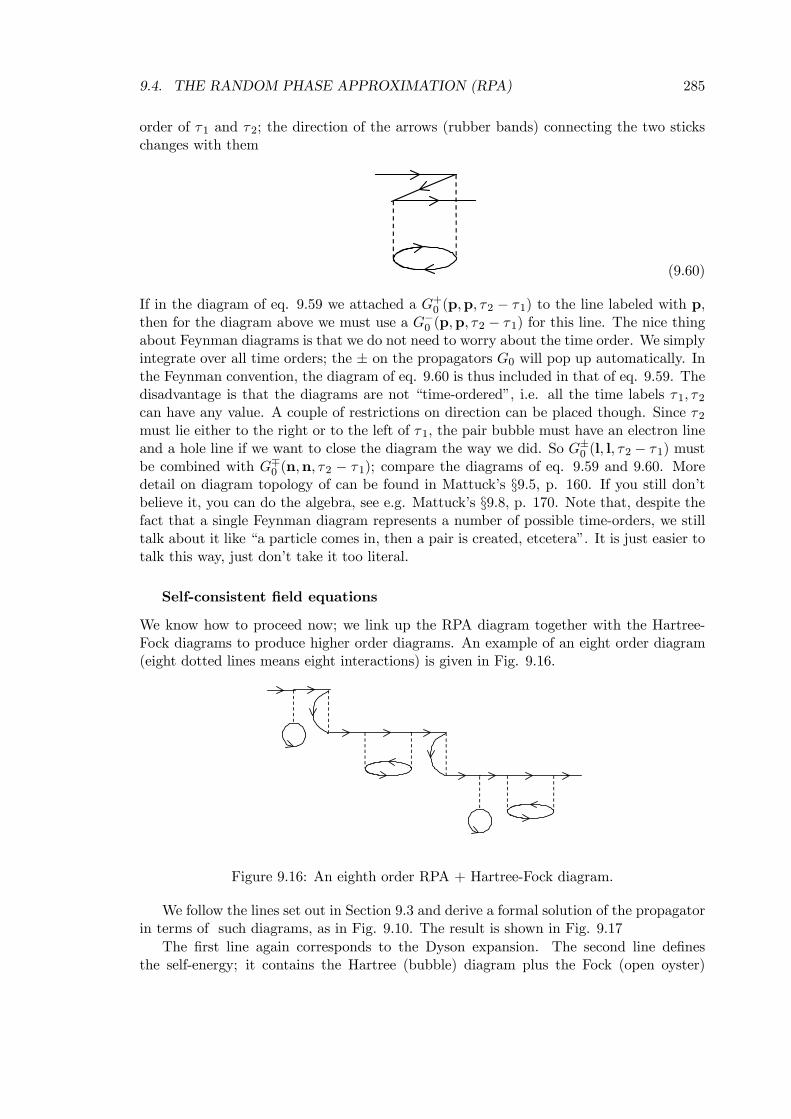
9.4. THE RANDOM PHASE APPROXIMATION (RPA) 285
order of τ1 and τ2; the direction of the arrows (rubber bands) connecting the two stickschanges with them
(9.60)
If in the diagram of eq. 9.59 we attached a G+0 (p,p, τ2 − τ1) to the line labeled with p,then for the diagram above we must use a G−0 (p,p, τ2 − τ1) for this line. The nice thingabout Feynman diagrams is that we do not need to worry about the time order. We simplyintegrate over all time orders; the ± on the propagators G0 will pop up automatically. Inthe Feynman convention, the diagram of eq. 9.60 is thus included in that of eq. 9.59. Thedisadvantage is that the diagrams are not “time-ordered”, i.e. all the time labels τ1, τ2can have any value. A couple of restrictions on direction can be placed though. Since τ2must lie either to the right or to the left of τ1, the pair bubble must have an electron lineand a hole line if we want to close the diagram the way we did. So G±0 (l, l, τ2 − τ1) mustbe combined with G∓0 (n,n, τ2 − τ1); compare the diagrams of eq. 9.59 and 9.60. Moredetail on diagram topology of can be found in Mattuck’s §9.5, p. 160. If you still don’tbelieve it, you can do the algebra, see e.g. Mattuck’s §9.8, p. 170. Note that, despite thefact that a single Feynman diagram represents a number of possible time-orders, we stilltalk about it like “a particle comes in, then a pair is created, etcetera”. It is just easier totalk this way, just don’t take it too literal.
Self-consistent field equations
We know how to proceed now; we link up the RPA diagram together with the Hartree-Fock diagrams to produce higher order diagrams. An example of an eight order diagram(eight dotted lines means eight interactions) is given in Fig. 9.16.
Figure 9.16: An eighth order RPA + Hartree-Fock diagram.
We follow the lines set out in Section 9.3 and derive a formal solution of the propagatorin terms of such diagrams, as in Fig. 9.10. The result is shown in Fig. 9.17
The first line again corresponds to the Dyson expansion. The second line definesthe self-energy; it contains the Hartree (bubble) diagram plus the Fock (open oyster)
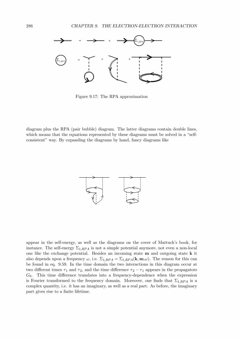
286 CHAPTER 9. THE ELECTRON-ELECTRON INTERACTION
= + RPA,1Σ
= +RPA,1Σ +
Figure 9.17: The RPA approximation
diagram plus the RPA (pair bubble) diagram. The latter diagrams contain double lines,which means that the equations represented by these diagrams must be solved in a “self-consistent” way. By expanding the diagrams by hand, fancy diagrams like
appear in the self-energy, as well as the diagrams on the cover of Mattuck’s book, forinstance. The self-energy Σ1,RPA is not a simple potential anymore, not even a non-localone like the exchange potential. Besides an incoming state m and outgoing state k italso depends upon a frequency ω, i.e. Σ1,RPA = Σ1,RPA(k,m,ω). The reason for this canbe found in eq. 9.59. In the time domain the two interactions in this diagram occur attwo different times τ1 and τ2, and the time difference τ2 − τ1 appears in the propagatorsG0. This time difference translates into a frequency-dependence when the expressionis Fourier transformed to the frequency domain. Moreover, one finds that Σ1,RPA is acomplex quantity, i.e. it has an imaginary, as well as a real part. As before, the imaginarypart gives rise to a finite lifetime.
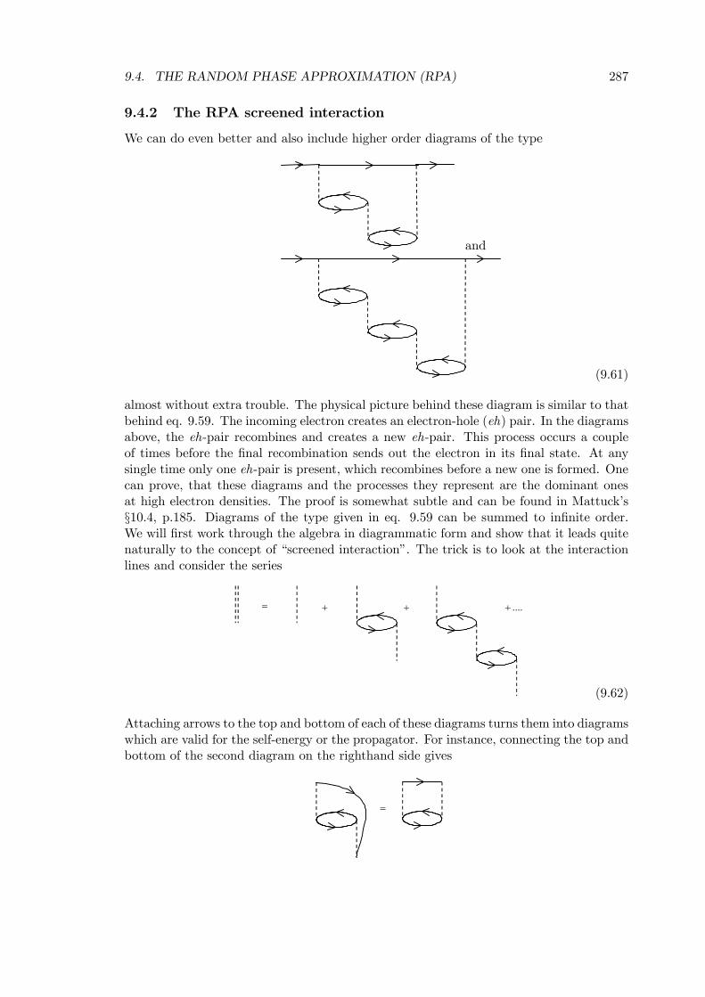
9.4. THE RANDOM PHASE APPROXIMATION (RPA) 287
9.4.2 The RPA screened interaction
We can do even better and also include higher order diagrams of the type
and
(9.61)
almost without extra trouble. The physical picture behind these diagram is similar to thatbehind eq. 9.59. The incoming electron creates an electron-hole (eh) pair. In the diagramsabove, the eh-pair recombines and creates a new eh-pair. This process occurs a coupleof times before the final recombination sends out the electron in its final state. At anysingle time only one eh-pair is present, which recombines before a new one is formed. Onecan prove, that these diagrams and the processes they represent are the dominant onesat high electron densities. The proof is somewhat subtle and can be found in Mattuck’s§10.4, p.185. Diagrams of the type given in eq. 9.59 can be summed to infinite order.We will first work through the algebra in diagrammatic form and show that it leads quitenaturally to the concept of “screened interaction”. The trick is to look at the interactionlines and consider the series
= + + ....+
(9.62)
Attaching arrows to the top and bottom of each of these diagrams turns them into diagramswhich are valid for the self-energy or the propagator. For instance, connecting the top andbottom of the second diagram on the righthand side gives
=
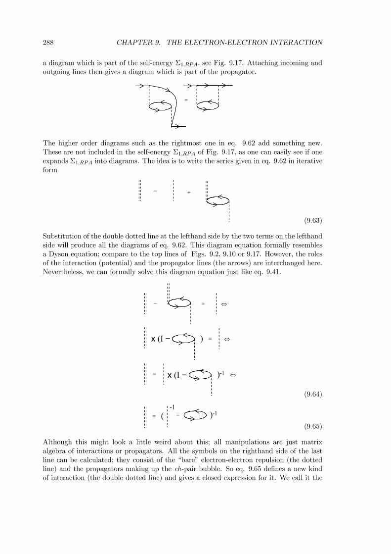
288 CHAPTER 9. THE ELECTRON-ELECTRON INTERACTION
a diagram which is part of the self-energy Σ1,RPA, see Fig. 9.17. Attaching incoming andoutgoing lines then gives a diagram which is part of the propagator.
=
The higher order diagrams such as the rightmost one in eq. 9.62 add something new.These are not included in the self-energy Σ1,RPA of Fig. 9.17, as one can easily see if oneexpands Σ1,RPA into diagrams. The idea is to write the series given in eq. 9.62 in iterativeform
= +
(9.63)
Substitution of the double dotted line at the lefthand side by the two terms on the lefthandside will produce all the diagrams of eq. 9.62. This diagram equation formally resemblesa Dyson equation; compare to the top lines of Figs. 9.2, 9.10 or 9.17. However, the rolesof the interaction (potential) and the propagator lines (the arrows) are interchanged here.Nevertheless, we can formally solve this diagram equation just like eq. 9.41.
=− ⇔
x (I − ) = ⇔
= x (I − )-1 ⇔
(9.64)
= (-1
− )-1
(9.65)
Although this might look a little weird about this; all manipulations are just matrixalgebra of interactions or propagators. All the symbols on the righthand side of the lastline can be calculated; they consist of the “bare” electron-electron repulsion (the dottedline) and the propagators making up the eh-pair bubble. So eq. 9.65 defines a new kindof interaction (the double dotted line) and gives a closed expression for it. We call it the
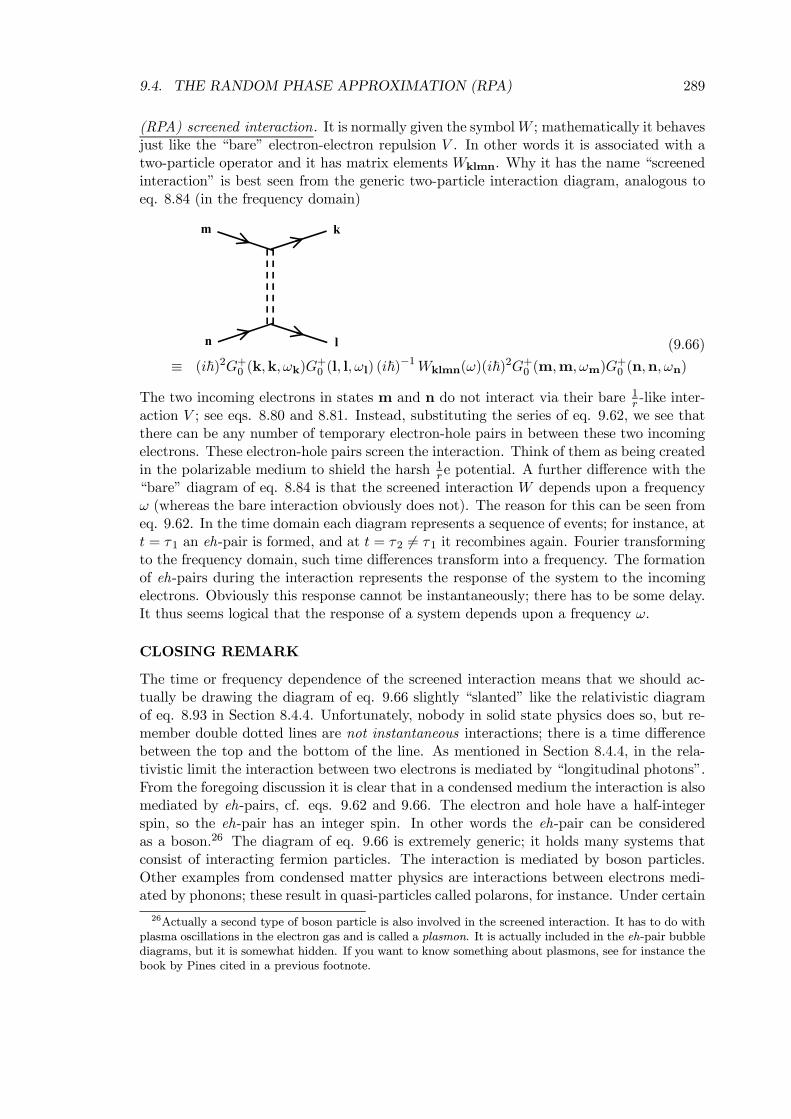
9.4. THE RANDOM PHASE APPROXIMATION (RPA) 289
(RPA) screened interaction. It is normally given the symbolW ; mathematically it behavesjust like the “bare” electron-electron repulsion V . In other words it is associated with atwo-particle operator and it has matrix elements Wklmn. Why it has the name “screenedinteraction” is best seen from the generic two-particle interaction diagram, analogous toeq. 8.84 (in the frequency domain)
l
km
n (9.66)
≡ (i~)2G+0 (k,k,ωk)G+0 (l, l,ωl) (i~)
−1Wklmn(ω)(i~)2G+0 (m,m,ωm)G+0 (n,n,ωn)
The two incoming electrons in states m and n do not interact via their bare 1r -like inter-
action V ; see eqs. 8.80 and 8.81. Instead, substituting the series of eq. 9.62, we see thatthere can be any number of temporary electron-hole pairs in between these two incomingelectrons. These electron-hole pairs screen the interaction. Think of them as being createdin the polarizable medium to shield the harsh 1
r e potential. A further difference with the“bare” diagram of eq. 8.84 is that the screened interaction W depends upon a frequencyω (whereas the bare interaction obviously does not). The reason for this can be seen fromeq. 9.62. In the time domain each diagram represents a sequence of events; for instance, att = τ1 an eh-pair is formed, and at t = τ2 6= τ1 it recombines again. Fourier transformingto the frequency domain, such time differences transform into a frequency. The formationof eh-pairs during the interaction represents the response of the system to the incomingelectrons. Obviously this response cannot be instantaneously; there has to be some delay.It thus seems logical that the response of a system depends upon a frequency ω.
CLOSING REMARK
The time or frequency dependence of the screened interaction means that we should ac-tually be drawing the diagram of eq. 9.66 slightly “slanted” like the relativistic diagramof eq. 8.93 in Section 8.4.4. Unfortunately, nobody in solid state physics does so, but re-member double dotted lines are not instantaneous interactions; there is a time differencebetween the top and the bottom of the line. As mentioned in Section 8.4.4, in the rela-tivistic limit the interaction between two electrons is mediated by “longitudinal photons”.From the foregoing discussion it is clear that in a condensed medium the interaction is alsomediated by eh-pairs, cf. eqs. 9.62 and 9.66. The electron and hole have a half-integerspin, so the eh-pair has an integer spin. In other words the eh-pair can be consideredas a boson.26 The diagram of eq. 9.66 is extremely generic; it holds many systems thatconsist of interacting fermion particles. The interaction is mediated by boson particles.Other examples from condensed matter physics are interactions between electrons medi-ated by phonons; these result in quasi-particles called polarons, for instance. Under certain
26Actually a second type of boson particle is also involved in the screened interaction. It has to do withplasma oscillations in the electron gas and is called a plasmon. It is actually included in the eh-pair bubblediagrams, but it is somewhat hidden. If you want to know something about plasmons, see for instance thebook by Pines cited in a previous footnote.
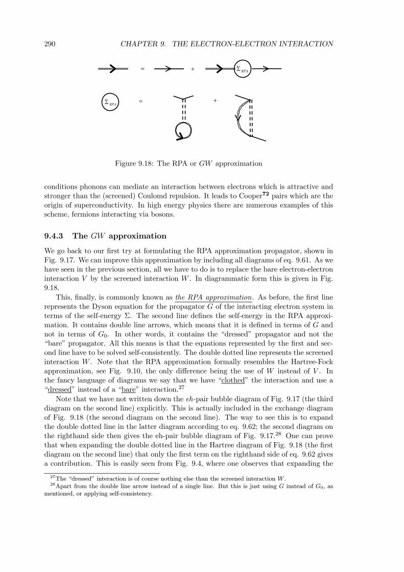
290 CHAPTER 9. THE ELECTRON-ELECTRON INTERACTION
= + RPAΣ
=RPAΣ +
Figure 9.18: The RPA or GW approximation
conditions phonons can mediate an interaction between electrons which is attractive andstronger than the (screened) Coulomd repulsion. It leads to Cooper72 pairs which are theorigin of superconductivity. In high energy physics there are numerous examples of thisscheme, fermions interacting via bosons.
9.4.3 The GW approximation
We go back to our first try at formulating the RPA approximation propagator, shown inFig. 9.17. We can improve this approximation by including all diagrams of eq. 9.61. As wehave seen in the previous section, all we have to do is to replace the bare electron-electroninteraction V by the screened interaction W . In diagrammatic form this is given in Fig.9.18.
This, finally, is commonly known as the RPA approximation. As before, the first linerepresents the Dyson equation for the propagator G of the interacting electron system interms of the self-energy Σ. The second line defines the self-energy in the RPA approxi-mation. It contains double line arrows, which means that it is defined in terms of G andnot in terms of G0. In other words, it contains the “dressed” propagator and not the“bare” propagator. All this means is that the equations represented by the first and sec-ond line have to be solved self-consistently. The double dotted line represents the screenedinteraction W . Note that the RPA approximation formally resembles the Hartree-Fockapproximation, see Fig. 9.10, the only difference being the use of W instead of V . Inthe fancy language of diagrams we say that we have “clothed” the interaction and use a“dressed” instead of a “bare” interaction.27
Note that we have not written down the eh-pair bubble diagram of Fig. 9.17 (the thirddiagram on the second line) explicitly. This is actually included in the exchange diagramof Fig. 9.18 (the second diagram on the second line). The way to see this is to expandthe double dotted line in the latter diagram according to eq. 9.62; the second diagram onthe righthand side then gives the eh-pair bubble diagram of Fig. 9.17.28 One can provethat when expanding the double dotted line in the Hartree diagram of Fig. 9.18 (the firstdiagram on the second line) that only the first term on the righthand side of eq. 9.62 givesa contribution. This is easily seen from Fig. 9.4, where one observes that expanding the
27The “dressed” interaction is of course nothing else than the screened interaction W .28Apart from the double line arrow instead of a single line. But this is just using G instead of G0, as
mentioned, or applying self-consistency.
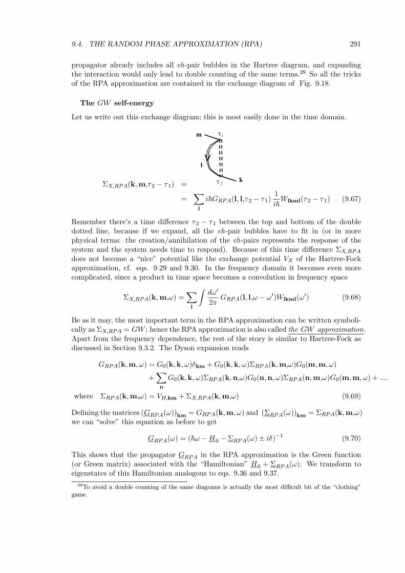
9.4. THE RANDOM PHASE APPROXIMATION (RPA) 291
propagator already includes all eh-pair bubbles in the Hartree diagram, and expandingthe interaction would only lead to double counting of the same terms.29 So all the tricksof the RPA approximation are contained in the exchange diagram of Fig. 9.18.
The GW self-energy
Let us write out this exchange diagram; this is most easily done in the time domain.
ΣX,RPA(k,m,τ2 − τ1) =
l
k
m 1τ
2τ
=Xl
i~GRPA(l, l,τ2 − τ1)1
i~Wlkml(τ2 − τ1) (9.67)
Remember there’s a time difference τ2 − τ1 between the top and bottom of the doubledotted line, because if we expand, all the eh-pair bubbles have to fit in (or in morephysical terms: the creation/annihilation of the eh-pairs represents the response of thesystem and the system needs time to respond). Because of this time difference ΣX,RPAdoes not become a “nice” potential like the exchange potential VX of the Hartree-Fockapproximation, cf. eqs. 9.29 and 9.30. In the frequency domain it becomes even morecomplicated, since a product in time space becomes a convolution in frequency space
ΣX,RPA(k,m,ω) =Xl
Zdω0
2πGRPA(l, l,ω − ω0)Wlkml(ω
0) (9.68)
Be as it may, the most important term in the RPA approximation can be written symboli-cally as ΣX,RPA = GW ; hence the RPA approximation is also called the GW approximation.Apart from the frequency dependence, the rest of the story is similar to Hartree-Fock asdiscussed in Section 9.3.2. The Dyson expansion reads
GRPA(k,m,ω) = G0(k,k,ω)δkm +G0(k,k,ω)ΣRPA(k,m,ω)G0(m,m,ω)
+Xn
G0(k,k,ω)ΣRPA(k,n,ω)G0(n,n,ω)ΣRPA(n,m,ω)G0(m,m,ω) + ....
where ΣRPA(k,m,ω) = VH,km +ΣX,RPA(k,m,ω) (9.69)
Defining the matrices (GRPA(ω))km = GRPA(k,m,ω) and (ΣRPA(ω))km = ΣRPA(k,m,ω)we can “solve” this equation as before to get
GRPA(ω) = (~ω −H0 − ΣRPA(ω)± iδ)−1 (9.70)
This shows that the propagator GRPA in the RPA approximation is the Green function(or Green matrix) associated with the “Hamiltonian” H0 + ΣRPA(ω). We transform toeigenstates of this Hamiltonian analogous to eqs. 9.36 and 9.37.
29To avoid a double counting of the same diagrams is actually the most difficult bit of the “clothing”game.
292 CHAPTER 9. THE ELECTRON-ELECTRON INTERACTION
The GW self-consistent field equations
As a result, one derives the GW (self consistent field) equations, which in wave functionform read like30"− ~2
2me∇2 −
XR
Ze2
|R− r| + VH(r)#ψn(r,ω) +
Zd3r0ΣX,RPA(r, r0,ω)ψn(r
0,ω) = ²n(ω)ψn(r,ω)
(9.71)
where, similar to the Hartree-Fock case the self-energy ΣX,RPA(r, r0,ω) in the position
representation is defined by
ΣX,RPA(k,m,ω) =
Z Zd3r d3r0 ψ∗k(r,ω)ΣX,RPA(r, r
0,ω)ψm(r0,ω)⇔
ΣX,RPA(r, r0,ω) =
Xk,m
ψk(r,ω)ΣX,RPA(k,m,ω)ψ∗m(r
0,ω) (9.72)
Note how the ω-dependence of ΣX,RPA adds an ω-dependence to the GW -“orbitals”ψn(r,ω) and their “energies” ²n(ω). Most of this frequency-dependence is boring andnot of interest. Let me try to explain what I mean. Analogous to eq. 9.39, the propagatorin the RPA approximation on the basis of the states which are the solution of eq. 9.71,has a simple diagonal form
GRPA(k,n,ω) = δkn1
~ω − ²k(ω)± iδ (9.73)
where ²k(ω) are the eigenvalues of eq. 9.71. As always, in the end the propagator in thetime domain is the quantity that we want. Remember, it gives the probability amplitudethat a particle which is created in a state n at some initial time, is found in a state k atsome later time. To get to the time domain we have to Fourier transform eq. 9.73, like wediscussed in the previous chapter and in Section 4; see in particular Section 4.4 and thediscussion following eq. 4.35. We know from this discussion that the poles of the functionGRPA(k,n,ω) determine the behaviour of its Fourier transform. At these poles we have
~ω − ²k(ω) = 0 (9.74)
We now assume that the functions ²k(ω) are simple and well-behaved (monotonic, forinstance). Then eq. 9.74 has only one solution for each ²k; call this solution ω = ωk.This assumption is called the quasi-particle ansatz . It can be proven in some cases.In any case one expects it to be true if the ω-dependence of ΣX,RPA is rather weak.
31
This is “normally” the case, and systems for which it is true are called normal Fermiliquids (or gases). Exceptions are called “strongly correlated systems”. So for a “nor-mal” system only the points ω = ωk are of interest. The functions ψk(r,ωk) are thencalled the quasi-particle wave functions or orbitals and the energies ²k(ωk) are called thequasi-particle eigenvalues (eq. 9.71 is then called the quasi-particle wave equation). Ingeneral, the self-energy ΣX,RPA is complex (it has an imaginary, as well as a real part);
30as far as I am concerned you may also call them the RPA equations, since it’s the same thing.31If ΣX does not depend on ω at all we are back at the Hartree-Fock case again, where ²k is also
independent of ω, and for sure eq. 9.74 has only one solution.
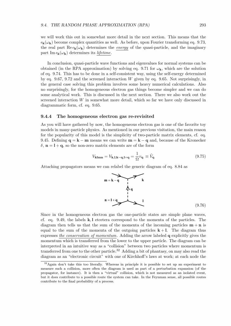
9.4. THE RANDOM PHASE APPROXIMATION (RPA) 293
we will work this out in somewhat more detail in the next section. This means that the²k(ωk) become complex quantities as well. As before, upon Fourier transforming eq. 9.73,the real part Re ²k(ωk) determines the energy of the quasi-particle, and the imaginarypart Im ²k(ωk) determines its lifetime.
In conclusion, quasi-particle wave functions and eigenvalues for normal systems can beobtained (in the RPA approximation) by solving eq. 9.71 for ωk, which are the solutionof eq. 9.74. This has to be done in a self-consistent way, using the self-energy determinedby eq. 9.67, 9.72 and the screened interaction W given by eq. 9.65. Not surprisingly, inthe general case solving this problem involves some heavy numerical calculations. Alsono surprisingly, for the homogeneous electron gas things become simpler and we can dosome analytical work. This is discussed in the next section. There we also work out thescreened interaction W in somewhat more detail, which so far we have only discussed indiagrammatic form, cf. eq. 9.65.
9.4.4 The homogeneous electron gas re-revisited
As you will have gathered by now, the homogeneous electron gas is one of the favorite toymodels in many-particle physics. As mentioned in our previous visitation, the main reasonfor the popularity of this model is the simplicity of two-particle matrix elements, cf. eq.9.45. Defining q = k−m means we can write m = k− q and, because of the Kroneckerδ, n = l+ q, so the non-zero matrix elements are of the form
Vklmn = Vk,l,k−q,l+q =1
Ωvq ≡ Vq (9.75)
Attaching propagators means we can relabel the generic diagram of eq. 8.84 as
l
kqkm −=
qln +=
q
(9.76)
Since in the homogeneous electron gas the one-particle states are simple plane waves,cf. eq. 9.49, the labels k, l etcetera correspond to the momenta of the particles. Thediagram then tells us that the sum of the momenta of the incoming particles m+ n isequal to the sum of the momenta of the outgoing particles k+ l. The diagram thusexpresses the conservation of momentum. Adding the arrow labeled q explicitly gives themomentum which is transferred from the lower to the upper particle. The diagram can beinterpreted in an intuitive way as a “collision” between two particles where momentum istransferred from one to the other particle.32 Adding a bit of phantasy, on may also read thediagram as an “electronic circuit” with one of Kirchhoff’s laws at work; at each node the
32Again don’t take this too literally. Whereas in principle it is possible to set up an experiment tomeasure such a collision, more often the diagram is used as part of a perturbation expansion (of thepropagator, for instance). It is then a “virtual” collision, which is not measured as an isolated event,but it does contribute to a possible route the system can take. In the Feynman sense, all possible routescontribute to the final probability of a process.
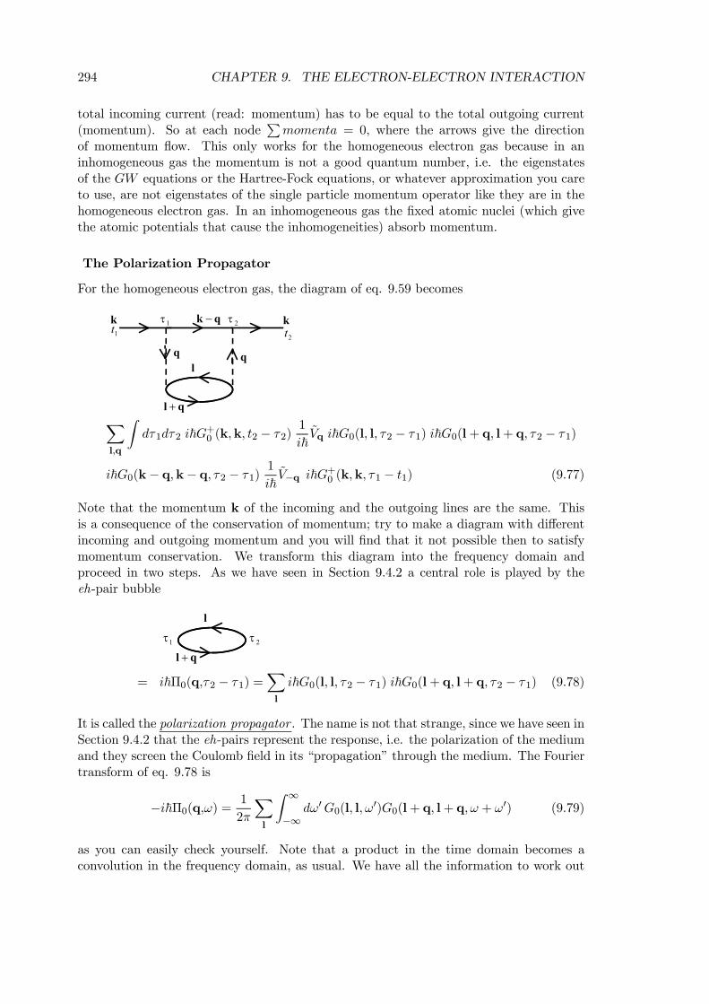
294 CHAPTER 9. THE ELECTRON-ELECTRON INTERACTION
total incoming current (read: momentum) has to be equal to the total outgoing current(momentum). So at each node
Pmomenta = 0, where the arrows give the direction
of momentum flow. This only works for the homogeneous electron gas because in aninhomogeneous gas the momentum is not a good quantum number, i.e. the eigenstatesof the GW equations or the Hartree-Fock equations, or whatever approximation you careto use, are not eigenstates of the single particle momentum operator like they are in thehomogeneous electron gas. In an inhomogeneous gas the fixed atomic nuclei (which givethe atomic potentials that cause the inhomogeneities) absorb momentum.
The Polarization Propagator
For the homogeneous electron gas, the diagram of eq. 9.59 becomes
k1t
k2t
ql +
l
qk −1τ 2τ
Xl,q
Zdτ1dτ2 i~G+0 (k,k, t2 − τ2)
1
i~Vq i~G0(l, l, τ2 − τ1) i~G0(l+ q, l+ q, τ2 − τ1)
i~G0(k− q,k− q, τ2 − τ1)1
i~V−q i~G+0 (k,k, τ1 − t1) (9.77)
Note that the momentum k of the incoming and the outgoing lines are the same. Thisis a consequence of the conservation of momentum; try to make a diagram with differentincoming and outgoing momentum and you will find that it not possible then to satisfymomentum conservation. We transform this diagram into the frequency domain andproceed in two steps. As we have seen in Section 9.4.2 a central role is played by theeh-pair bubble
ql +
l
1τ 2τ
= i~Π0(q,τ2 − τ1) =Xl
i~G0(l, l, τ2 − τ1) i~G0(l+ q, l+ q, τ2 − τ1) (9.78)
It is called the polarization propagator . The name is not that strange, since we have seen inSection 9.4.2 that the eh-pairs represent the response, i.e. the polarization of the mediumand they screen the Coulomb field in its “propagation” through the medium. The Fouriertransform of eq. 9.78 is
−i~Π0(q,ω) = 1
2π
Xl
Z ∞
−∞dω0G0(l, l,ω0)G0(l+ q, l+ q,ω + ω0) (9.79)
as you can easily check yourself. Note that a product in the time domain becomes aconvolution in the frequency domain, as usual. We have all the information to work out
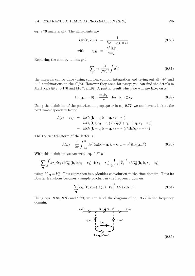
9.4. THE RANDOM PHASE APPROXIMATION (RPA) 295
eq. 9.79 analytically. The ingredients are
G±0 (k,k,ω) =1
~ω − ²0,k ± iδ (9.80)
with ²0,k =~2 |k|22me
Replacing the sum by an integral Xl
→ Ω
(2π)2
Zd3l (9.81)
the integrals can be done (using complex contour integration and trying out all “+” and“−” combinations on the G0’s). However they are a bit nasty; you can find the details inMattuck’s §9.8, p.170 and §10.7, p.197. A partial result which we will use later on is
Π0(q,ω = 0) =mekFπ
for |q| ¿ kF (9.82)
Using the definition of the polarization propagator in eq. 9.77, we can have a look at thenext time-dependent factor
A(τ2 − τ1) = i~G0(k− q,k− q, τ2 − τ1)
i~G0(l, l, τ2 − τ1) i~G0(l+ q, l+ q, τ2 − τ1)
= i~G0(k− q,k− q, τ2 − τ1)i~Π0(q,τ2 − τ1)
The Fourier transform of the latter is
A(ω) =1
2π
Z ∞
−∞dω00G0(k− q,k− q,ω − ω00)Π0(q,ω00) (9.83)
With this definition we can write eq. 9.77 asXq
Zdτ1dτ2 i~G+0 (k,k, t2 − τ2) A(τ2 − τ1)
1
(i~)2¯Vq
¯2i~G+0 (k,k, τ1 − t1)
using V−q = V ∗q . This expression is a (double) convolution in the time domain. Thus itsFourier transform becomes a simple product in the frequency domainX
q
G+0 (k,k,ω) A(ω)¯Vq
¯2G+0 (k,k,ω) (9.84)
Using eqs. 9.84, 9.83 and 9.79, we can label the diagram of eq. 9.77 in the frequencydomain.
ω,k ω,k
''', ωω ++ ql
',ωl
'', ωω −− qk
'',ωq'',ωq
(9.85)
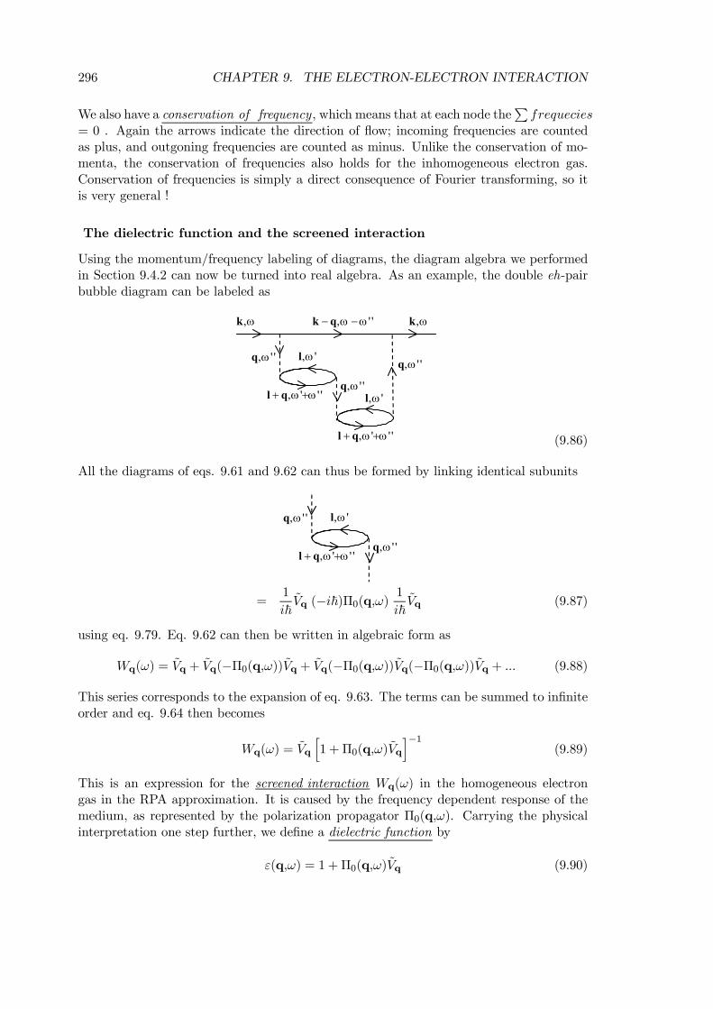
296 CHAPTER 9. THE ELECTRON-ELECTRON INTERACTION
We also have a conservation of frequency, which means that at each node thePfrequecies
= 0 . Again the arrows indicate the direction of flow; incoming frequencies are countedas plus, and outgoning frequencies are counted as minus. Unlike the conservation of mo-menta, the conservation of frequencies also holds for the inhomogeneous electron gas.Conservation of frequencies is simply a direct consequence of Fourier transforming, so itis very general !
The dielectric function and the screened interaction
Using the momentum/frequency labeling of diagrams, the diagram algebra we performedin Section 9.4.2 can now be turned into real algebra. As an example, the double eh-pairbubble diagram can be labeled as
ω,k ω,k'', ωω −− qk
'',ωq
'',ωq
'',ωq',ωl
',ωl''', ωω ++ ql
''', ωω ++ ql (9.86)
All the diagrams of eqs. 9.61 and 9.62 can thus be formed by linking identical subunits
'',ωq
'',ωq
',ωl
''', ωω ++ ql
=1
i~Vq (−i~)Π0(q,ω) 1
i~Vq (9.87)
using eq. 9.79. Eq. 9.62 can then be written in algebraic form as
Wq(ω) = Vq + Vq(−Π0(q,ω))Vq + Vq(−Π0(q,ω))Vq(−Π0(q,ω))Vq + ... (9.88)
This series corresponds to the expansion of eq. 9.63. The terms can be summed to infiniteorder and eq. 9.64 then becomes
Wq(ω) = Vq
h1 +Π0(q,ω)Vq
i−1(9.89)
This is an expression for the screened interaction Wq(ω) in the homogeneous electrongas in the RPA approximation. It is caused by the frequency dependent response of themedium, as represented by the polarization propagator Π0(q,ω). Carrying the physicalinterpretation one step further, we define a dielectric function by
ε(q,ω) = 1 +Π0(q,ω)Vq (9.90)
9.4. THE RANDOM PHASE APPROXIMATION (RPA) 297
so the screened interaction becomes
Wq(ω) =Vq
ε(q,ω)(9.91)
Inside a medium one does not experience the bare Coulomb potential Vq but one that isdielectrically screened by ε(q,ω). Fourier transforming eq. 9.91 to real space and the timedomain on gets
W (r,t) ∝Zdωeiωt
Zd3qeiq·rWq(ω)
=
Z Zε−1(r− r0,t− t0)V (r0)d3r0dt0
=
Z Zε−1(r− r0,t− t0)e
2
r0d3r0dt0 (9.92)
Note again that a simple product in momentum/frequency space like eq. 9.91 becomesa convolution in real/time space. Screening is a non-local, time-dependent effect, as youundoubtedly know from your electrodynamics course.
Simple screening for metals and isolators
If the perturbing potential does not vary tto much over microscopic distances, and itsfrequency is small compared to the natural response frequencies of the system, we mayapproximate the dielectric function by a constant ε(q,ω) ≈ εe = ε(q = 0,ω = 0), which iscalled the (static) dielectric constant. Such an approximation is not sufficiently accuratefor microscopic potentials, but we can use the idea to get a first look and feel for the physicsinvolved. In case of metallic screening εe = ∞, so we must do a little better from thestart. We consider a static polarization function, eq. 9.82.33 The bare electron-electronCoulomb repulsion and its Fourier transform are given by (see Mattuck p. 191; in cgsunits, I am sorry for that)
V (r) =e2
r↔ vq =
4πe2
q2(9.93)
From eqs. 9.82, 9.90 and 9.93, one obtains for the static, ω = 0, and long wave lengthq ¿ kF limit
ε(q,0) = 1 +λ2
q2with
λ2 =4mee
2kFπ
= 4mee2(3ρ
π)13 (9.94)
where ρ is the density of the electron gas. Using this expression for all wave vectors q (al-though stricktly speaking one should not do that) is called the Thomas-Fermi model for screening .We find for the screened interaction, eq. 9.91 and its Fourier transform
Wq(ω = 0) =4πe2
q2 + λ2↔W (r,ω = 0) =
e2
re−λr (9.95)
33The exact expression for Π0(q,ω) can be obtained, but it is not very enlighting due to its complexity,see e.g. Fetter & Walecka. For simplicity reasons we therefore stick to the static approximation.
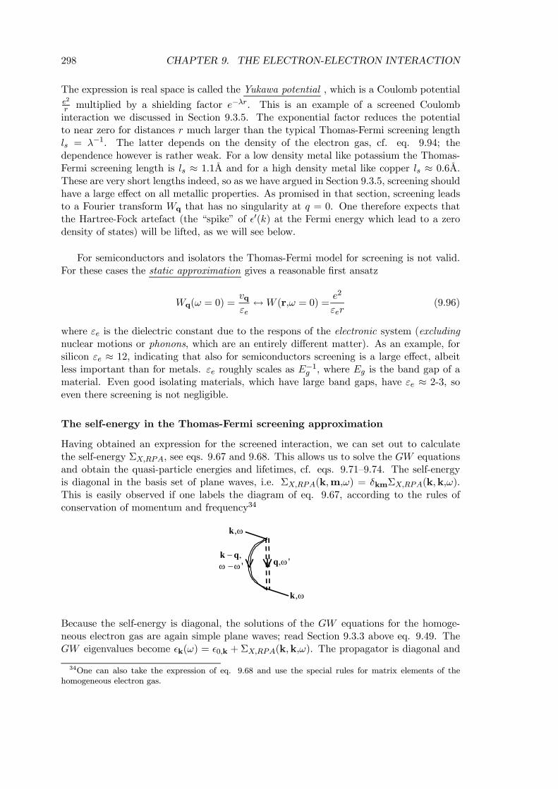
298 CHAPTER 9. THE ELECTRON-ELECTRON INTERACTION
The expression is real space is called the Yukawa potential , which is a Coulomb potentiale2
r multiplied by a shielding factor e−λr. This is an example of a screened Coulombinteraction we discussed in Section 9.3.5. The exponential factor reduces the potentialto near zero for distances r much larger than the typical Thomas-Fermi screening lengthls = λ−1. The latter depends on the density of the electron gas, cf. eq. 9.94; thedependence however is rather weak. For a low density metal like potassium the Thomas-Fermi screening length is ls ≈ 1.1A and for a high density metal like copper ls ≈ 0.6A.These are very short lengths indeed, so as we have argued in Section 9.3.5, screening shouldhave a large effect on all metallic properties. As promised in that section, screening leadsto a Fourier transform Wq that has no singularity at q = 0. One therefore expects thatthe Hartree-Fock artefact (the “spike” of ²0(k) at the Fermi energy which lead to a zerodensity of states) will be lifted, as we will see below.
For semiconductors and isolators the Thomas-Fermi model for screening is not valid.For these cases the static approximation gives a reasonable first ansatz
Wq(ω = 0) =vqεe↔W (r,ω = 0) =
e2
εer(9.96)
where εe is the dielectric constant due to the respons of the electronic system (excludingnuclear motions or phonons, which are an entirely different matter). As an example, forsilicon εe ≈ 12, indicating that also for semiconductors screening is a large effect, albeitless important than for metals. εe roughly scales as E
−1g , where Eg is the band gap of a
material. Even good isolating materials, which have large band gaps, have εe ≈ 2-3, soeven there screening is not negligible.
The self-energy in the Thomas-Fermi screening approximation
Having obtained an expression for the screened interaction, we can set out to calculatethe self-energy ΣX,RPA, see eqs. 9.67 and 9.68. This allows us to solve the GW equationsand obtain the quasi-particle energies and lifetimes, cf. eqs. 9.71—9.74. The self-energyis diagonal in the basis set of plane waves, i.e. ΣX,RPA(k,m,ω) = δkmΣX,RPA(k,k,ω).This is easily observed if one labels the diagram of eq. 9.67, according to the rules ofconservation of momentum and frequency34
ω,k
ω,k
',ωq,qk −'ωω −
Because the self-energy is diagonal, the solutions of the GW equations for the homoge-neous electron gas are again simple plane waves; read Section 9.3.3 above eq. 9.49. TheGW eigenvalues become ²k(ω) = ²0,k + ΣX,RPA(k,k,ω). The propagator is diagonal and
34One can also take the expression of eq. 9.68 and use the special rules for matrix elements of thehomogeneous electron gas.
9.4. THE RANDOM PHASE APPROXIMATION (RPA) 299
becomes
GRPA(k,k,ω) =1
~ω − ²k(ω)± iδ =1
~ω − ²0,k −ΣX,RPA(k,k,ω)± iδ (9.97)
The self-energy according to eq. 9.68 becomes
ΣX,RPA(k,k,ω) =Xq
Zdω0
2πGRPA(k− q,k− q,ω − ω0)Wq(ω
0) (9.98)
Making the usual substition, cf. eq. 9.81 and using eq.9.73, 9.75 and 9.91 we get
ΣX,RPA(k,k,ω) =
Zd3q
(2π)3
Zdω0
2π
Wq(ω0)
~(ω − ω0)− ²k−q(ω − ω0)± iδ where (9.99)
²l(ω) = ²0,l +ΣX,RPA(l, l,ω) and
Wq(ω) =vq
ε(q,ω)
Note the occurence of ΣX,RPA both on the righthand and on the lefthand side of eq. 9.99.This again is a matter of self-consistency; it is an equation that is to be solved iteratively.35
The integrals can in principle be attacked, but they are extremely nasty and we will notpursue them here. We can get some physical look and feel however by studying a limitingcase. For instance, we can start by setting ΣX,RPA to zero on the righthand side of eq.9.99. This is equivalent to using G0 instead of GRPA on the righthand side of eq. 9.98,or, in other words, doing a non self-consistent calculation. We then approximate Wq(ω
0)by its static value Wq(0) of eq. 9.95, which uses the Thomas-Fermi model for screening,and get
ΣTFX,RPA(k,k,ω) ≈Z
d3q
(2π)34πe2
q2 + λ2
Zdω0
2π
1
~ω00 − ²0,k−q ± iδ
= −Z|k−q|≤kF
d3q
(2π)34πe2
q2 + λ2=
Zq0≤kF
d3q0
(2π)34πe2¯
k− q0¯2 + λ2(9.100)
where the TF superscript indicates that we have used the Thomas-Fermi model for staticscreening. Defining ω00 = ω − ω0, the frequency integral has to be done with +iδ forelectrons, |k− q| > kF , and −iδ for holes, |k− q| ≤ kF . As in the Hartree-Fock case onlythe occupied states |k− q| ≤ kF give a contribution, which makes sense since an incomingparticle can only interact with particles in the system that are present (and if present,they occupy a state). The second line of this equation can then be derived using a contourintegration on the frequency integral (see Mattuck’s Appendix I and the discussion of hiseq. (4.31) and (8.35)). Note that the frequency dependence is now gone on the righthandside, as one expects from a static approximation. The remaining integral
Rd3q0can be
done, see Mattuck’s p. 93-94, or use MAPLE. The result is the following rather unwieldyexpression
ΣTFX,RPA(k,k) = −e2
π 14k
¡k2F − k2 + λ2
¢ ·ln
µ(k + kF )
2 + λ2
(k − kF )2 + λ2
¶¸+kF − λ
·arctan
k + kFλ
− arctan k − kFλ
¸ (9.101)
35For instance, start by setting ΣX,RPA = 0 in the righthand side. This gives a Σ(1)X,RPA on the lefthand
side. Use this solution in the righthand side to obtain a Σ(2)X,RPA on the lefthand side, etcetera. When
Σ(N+1)X,RPA = Σ
(N)X,RPA we have a self-consistent solution.
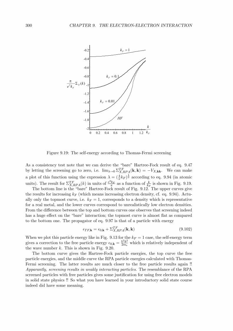
300 CHAPTER 9. THE ELECTRON-ELECTRON INTERACTION
-2
-1.8
-1.6
-1.4
-1.2
-1
-0.8
-0.6
-0.4
-0.2
0 0.2 0.4 0.6 0.8 1 1.2k
)(2 kke XF
Σπ
Fkk
1=Fk
1.0=Fk
01.0=Fk
HF
Figure 9.19: The self-energy according to Thomas-Fermi screening
As a consistency test note that we can derive the “bare” Hartree-Fock result of eq. 9.47by letting the screening go to zero, i.e. limλ→0ΣTFX,RPA(k,k) = −VX,kk. We can make
a plot of this function using the expression λ = ( 4πkF )12 according to eq. 9.94 (in atomic
units). The result for ΣTFX,RPA(k) in units ofe2kFπ as a function of k
kFis shown in Fig. 9.19.
The bottom line is the “bare” Hartree-Fock result of Fig. 9.12. The upper curves givethe results for increasing kF (which means increasing electron density, cf. eq. 9.94). Actu-ally only the topmost curve, i.e. kF = 1, corresponds to a density which is representativefor a real metal, and the lower curves correspond to unrealistically low electron densities.From the difference between the top and bottom curves one observes that screening indeedhas a huge effect on the “bare” interaction; the topmost curve is almost flat as comparedto the bottom one. The propagator of eq. 9.97 is that of a particle with energy
²TF,k = ²0,k +ΣTFX,RPA(k,k) (9.102)
When we plot this particle energy like in Fig. 9.13 for the kF = 1 case, the self-energy termgives a correction to the free particle energy ²0,k =
~2k22me
which is relatively independent ofthe wave number k. This is shown in Fig. 9.20.
The bottom curve gives the Hartree-Fock particle energies, the top curve the freeparticle energies, and the middle curve the RPA particle energies calculated with Thomas-Fermi screening. The latter results are much closer to the free particle results again !!Apparantly, screening results in weakly interacting particles. The resemblance of the RPAscreened particles with free particles gives some justification for using free electron modelsin solid state physics !! So what you have learned in your introductory solid state courseindeed did have some meaning.
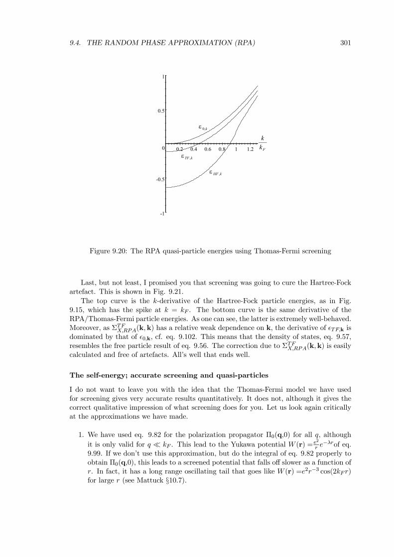
9.4. THE RANDOM PHASE APPROXIMATION (RPA) 301
-1
-0.5
0
0.5
1
0.2 0.4 0.6 0.8 1 1.2k
Fkk
k,0ε
kHF ,ε
kTF ,ε
Figure 9.20: The RPA quasi-particle energies using Thomas-Fermi screening
Last, but not least, I promised you that screening was going to cure the Hartree-Fockartefact. This is shown in Fig. 9.21.
The top curve is the k-derivative of the Hartree-Fock particle energies, as in Fig.9.15, which has the spike at k = kF . The bottom curve is the same derivative of theRPA/Thomas-Fermi particle energies. As one can see, the latter is extremely well-behaved.Moreover, as ΣTFX,RPA(k,k) has a relative weak dependence on k, the derivative of ²TF,k isdominated by that of ²0,k, cf. eq. 9.102. This means that the density of states, eq. 9.57,resembles the free particle result of eq. 9.56. The correction due to ΣTFX,RPA(k,k) is easilycalculated and free of artefacts. All’s well that ends well.
The self-energy; accurate screening and quasi-particles
I do not want to leave you with the idea that the Thomas-Fermi model we have usedfor screening gives very accurate results quantitatively. It does not, although it gives thecorrect qualitative impression of what screening does for you. Let us look again criticallyat the approximations we have made.
1. We have used eq. 9.82 for the polarization propagator Π0(q,0) for all q, although
it is only valid for q ¿ kF . This lead to the Yukawa potential W (r) =e2
r e−λrof eq.
9.99. If we don’t use this approximation, but do the integral of eq. 9.82 properly toobtain Π0(q,0), this leads to a screened potential that falls off slower as a function ofr. In fact, it has a long range oscillating tail that goes like W (r) =e2r−3 cos(2kF r)for large r (see Mattuck §10.7).
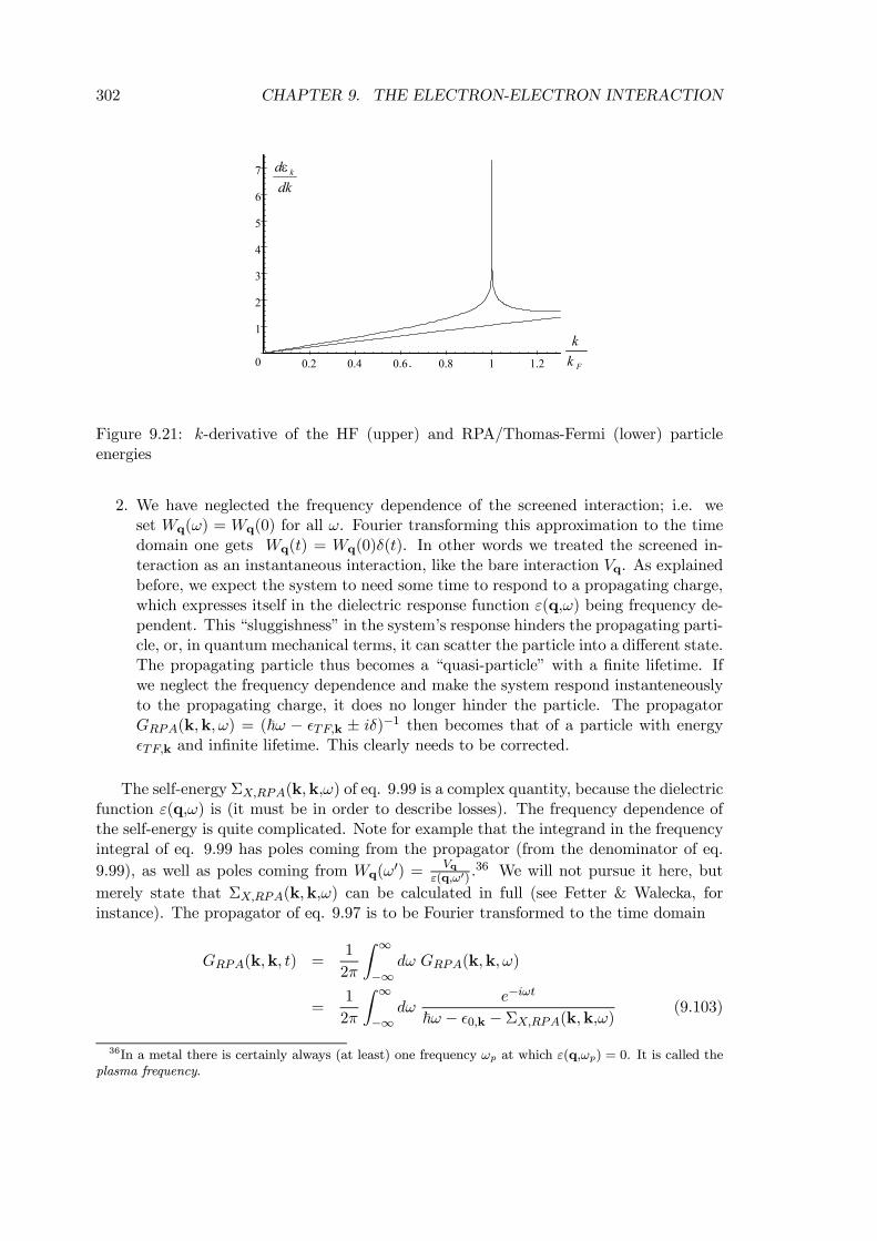
302 CHAPTER 9. THE ELECTRON-ELECTRON INTERACTION
0
1
2
3
4
5
6
7
0.2 0.4 0.6 0.8 1 1.2k
dkd kε
Fkk
Figure 9.21: k-derivative of the HF (upper) and RPA/Thomas-Fermi (lower) particleenergies
2. We have neglected the frequency dependence of the screened interaction; i.e. weset Wq(ω) = Wq(0) for all ω. Fourier transforming this approximation to the timedomain one gets Wq(t) = Wq(0)δ(t). In other words we treated the screened in-teraction as an instantaneous interaction, like the bare interaction Vq. As explainedbefore, we expect the system to need some time to respond to a propagating charge,which expresses itself in the dielectric response function ε(q,ω) being frequency de-pendent. This “sluggishness” in the system’s response hinders the propagating parti-cle, or, in quantum mechanical terms, it can scatter the particle into a different state.The propagating particle thus becomes a “quasi-particle” with a finite lifetime. Ifwe neglect the frequency dependence and make the system respond instanteneouslyto the propagating charge, it does no longer hinder the particle. The propagatorGRPA(k,k,ω) = (~ω − ²TF,k ± iδ)−1 then becomes that of a particle with energy²TF,k and infinite lifetime. This clearly needs to be corrected.
The self-energy ΣX,RPA(k,k,ω) of eq. 9.99 is a complex quantity, because the dielectricfunction ε(q,ω) is (it must be in order to describe losses). The frequency dependence ofthe self-energy is quite complicated. Note for example that the integrand in the frequencyintegral of eq. 9.99 has poles coming from the propagator (from the denominator of eq.
9.99), as well as poles coming from Wq(ω0) = Vq
ε(q,ω0) .36 We will not pursue it here, but
merely state that ΣX,RPA(k,k,ω) can be calculated in full (see Fetter & Walecka, forinstance). The propagator of eq. 9.97 is to be Fourier transformed to the time domain
GRPA(k,k, t) =1
2π
Z ∞
−∞dω GRPA(k,k,ω)
=1
2π
Z ∞
−∞dω
e−iωt
~ω − ²0,k − ΣX,RPA(k,k,ω) (9.103)
36In a metal there is certainly always (at least) one frequency ωp at which ε(q,ωp) = 0. It is called theplasma frequency.
9.4. THE RANDOM PHASE APPROXIMATION (RPA) 303
This is best done by complex contour integration, cf. Sections 4, 4.8.4. For that we needthe poles of the integrand. One can prove on rather formal grounds that the propagatorGRPA(k,k,ωc) as a function of a complex ωc = ω + iωi is analytical in the upper half ofthe complex plane for ~ω > ²F and in the lower half of the complex plane if ~ω < ²F . Inother words its poles must be in the lower half plane when ~ω > ²F and in the upper halfplane when ~ω < ²F .37 This then automatically means that
ImΣX,RPA(k,k,ω) < 0 for ~ω > ²FImΣX,RPA(k,k,ω) > 0 for ~ω < ²F (9.104)
According to Section 4.8, if we close the contour in the lower half plane we enclose thepoles which lie at ~ω > ²F , and get a non-zero result for t > 0
i~GRPA(k,k, t) = zke− i~ [²0,k+∆k]te−Γkt + F (k,t) for ²0,k +∆k > ²F ; t > 0(9.105)
where ∆k = ReΣX,RPA(k,k,ωk) and Γk =zk~|ImΣX,RPA(k,k,ωk)|
and zk =
µ1− ∂ΣX,RPA(k,k,ω)
∂ω|ω=ωk
¶−1and ~ωk − ²0,k − ΣX,RPA(k,k,ωk) = 0 determines the pole’s position. This resultmight seem a bit complicated, but start from the free particle case where the self-energyΣ = 0 per definition (which means ∆k = Γk = 0 and zk = 1). We have i~G0(k,k, t) =e−
i~ ²0,kt; ²0,k > ²F ; t > 0 which describes the free propagation of an electron. All the
effects of the electron-electron interaction have been worked into the self-energy Σ. Aswe observe in eq. 9.105, this results in (1) a shift of the energy level ²0,k → ²0,k + ∆k;(2) adding an exponential decay with a characteristic time τk = Γ
−1k and (3) adding a
weight factor zk. These are the same three features that appeared in the simple scatteringof one electron by interaction with atomic potentials in Section 4. Here they are causedby scattering due to electron-electron interaction. It seems that any kind of interactiongiving rise to scattering leads to a similar general behaviour for the propagation of theelectron. The seemingly new feature here is the function F (k,t); it takes care of otherpossible poles in the integration. For “normal” systems this function is smooth and hasa low weight, so it is not very important, for “strongly correlated” systems it may have amore complicated structure.
Since the propagator of eq. 9.105 resembles a free particle propagator, modified bythe three factors mentioned above, it is said to describe a quasi-particle (or in this casea quasi-electron, to be more precise). This term actually only makes sense if Γk is nottoo large or |zk| is too small, otherwise the quasi-particle would decay too fast or carrytoo small a weight to be observable in practice (this is usually measured experimentallyby (inverse) photoemission, Appendix II of the previous chapter). From eq. 9.104 one ob-serves that ImΣ(k,k,ω) changes sign at the Fermi level. One can prove that ImΣ(k,k,ω)
37The propagator must have poles somewhere, since otherwise the contour integration would give zeroaccording to the residue theorem, cf. section 4.8. Since we do have a particle or hole propagating, thepropagator obviously cannot be zero.This global statement of where the poles are holds in fact for the exact propagator G(k,k,ω) as well,
see Appendix II of the previous chapter; as well as for all the approximations we have encountered; thefree particle propagator G0(k,k,ω), eq. 9.14; the Hartree propagator GH(k,k,ω), eq. 9.26 and theHartree-Fock propagator GHF (k,k,ω), eq. 9.39.
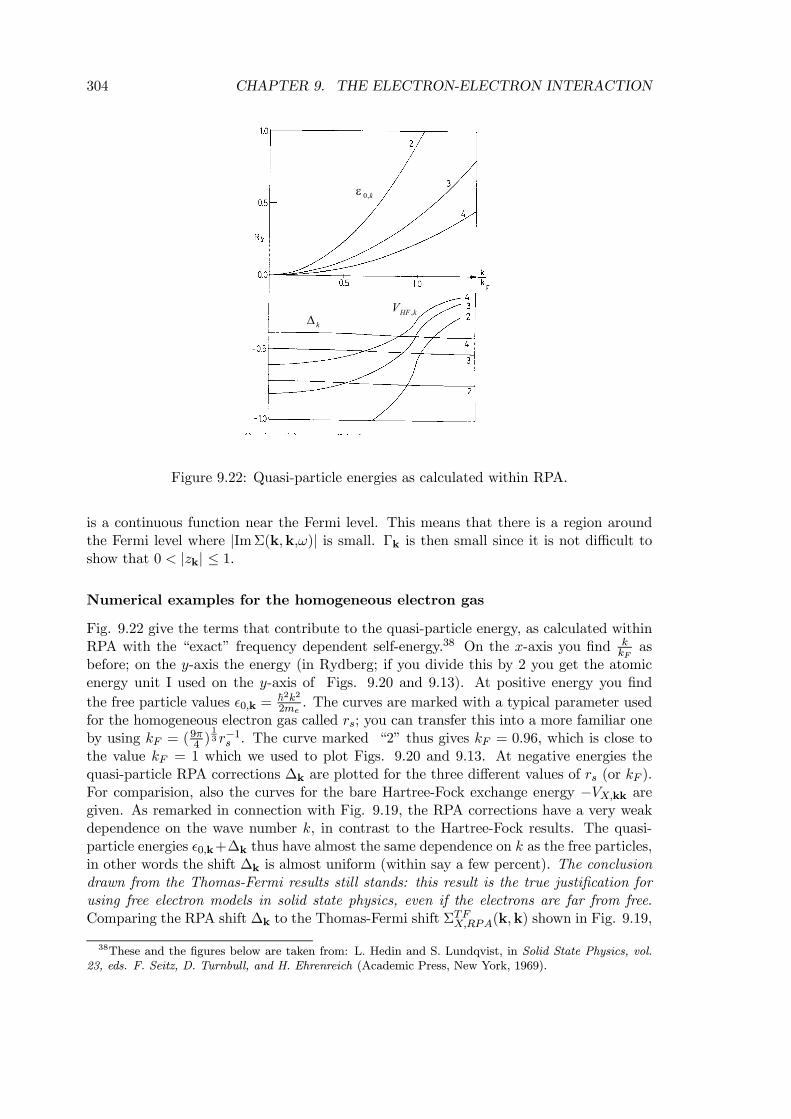
304 CHAPTER 9. THE ELECTRON-ELECTRON INTERACTION
k,0ε
k∆kHFV ,
Figure 9.22: Quasi-particle energies as calculated within RPA.
is a continuous function near the Fermi level. This means that there is a region aroundthe Fermi level where |ImΣ(k,k,ω)| is small. Γk is then small since it is not difficult toshow that 0 < |zk| ≤ 1.
Numerical examples for the homogeneous electron gas
Fig. 9.22 give the terms that contribute to the quasi-particle energy, as calculated withinRPA with the “exact” frequency dependent self-energy.38 On the x-axis you find k
kFas
before; on the y-axis the energy (in Rydberg; if you divide this by 2 you get the atomicenergy unit I used on the y-axis of Figs. 9.20 and 9.13). At positive energy you find
the free particle values ²0,k =~2k22me
. The curves are marked with a typical parameter usedfor the homogeneous electron gas called rs; you can transfer this into a more familiar oneby using kF = (
9π4 )
13 r−1s . The curve marked “2” thus gives kF = 0.96, which is close to
the value kF = 1 which we used to plot Figs. 9.20 and 9.13. At negative energies thequasi-particle RPA corrections ∆k are plotted for the three different values of rs (or kF ).For comparision, also the curves for the bare Hartree-Fock exchange energy −VX,kk aregiven. As remarked in connection with Fig. 9.19, the RPA corrections have a very weakdependence on the wave number k, in contrast to the Hartree-Fock results. The quasi-particle energies ²0,k+∆k thus have almost the same dependence on k as the free particles,in other words the shift ∆k is almost uniform (within say a few percent). The conclusiondrawn from the Thomas-Fermi results still stands: this result is the true justification forusing free electron models in solid state physics, even if the electrons are far from free.Comparing the RPA shift ∆k to the Thomas-Fermi shift Σ
TFX,RPA(k,k) shown in Fig. 9.19,
38These and the figures below are taken from: L. Hedin and S. Lundqvist, in Solid State Physics, vol.23, eds. F. Seitz, D. Turnbull, and H. Ehrenreich (Academic Press, New York, 1969).
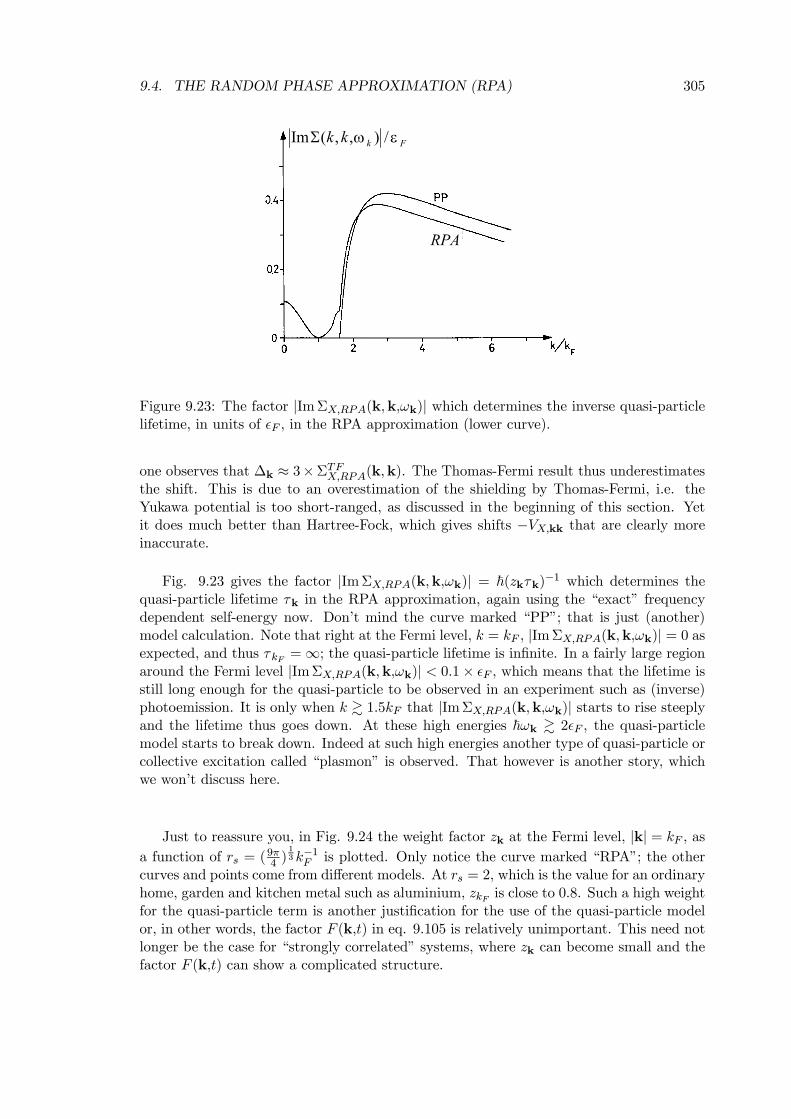
9.4. THE RANDOM PHASE APPROXIMATION (RPA) 305
Fkkk εω /),,(ImΣ
RPA
Figure 9.23: The factor |ImΣX,RPA(k,k,ωk)| which determines the inverse quasi-particlelifetime, in units of ²F , in the RPA approximation (lower curve).
one observes that ∆k ≈ 3×ΣTFX,RPA(k,k). The Thomas-Fermi result thus underestimatesthe shift. This is due to an overestimation of the shielding by Thomas-Fermi, i.e. theYukawa potential is too short-ranged, as discussed in the beginning of this section. Yetit does much better than Hartree-Fock, which gives shifts −VX,kk that are clearly moreinaccurate.
Fig. 9.23 gives the factor |ImΣX,RPA(k,k,ωk)| = ~(zkτk)−1 which determines thequasi-particle lifetime τk in the RPA approximation, again using the “exact” frequencydependent self-energy now. Don’t mind the curve marked “PP”; that is just (another)model calculation. Note that right at the Fermi level, k = kF , |ImΣX,RPA(k,k,ωk)| = 0 asexpected, and thus τkF =∞; the quasi-particle lifetime is infinite. In a fairly large regionaround the Fermi level |ImΣX,RPA(k,k,ωk)| < 0.1× ²F , which means that the lifetime isstill long enough for the quasi-particle to be observed in an experiment such as (inverse)photoemission. It is only when k & 1.5kF that |ImΣX,RPA(k,k,ωk)| starts to rise steeplyand the lifetime thus goes down. At these high energies ~ωk & 2²F , the quasi-particlemodel starts to break down. Indeed at such high energies another type of quasi-particle orcollective excitation called “plasmon” is observed. That however is another story, whichwe won’t discuss here.
Just to reassure you, in Fig. 9.24 the weight factor zk at the Fermi level, |k| = kF , asa function of rs = (
9π4 )
13 k−1F is plotted. Only notice the curve marked “RPA”; the other
curves and points come from different models. At rs = 2, which is the value for an ordinaryhome, garden and kitchen metal such as aluminium, zkF is close to 0.8. Such a high weightfor the quasi-particle term is another justification for the use of the quasi-particle modelor, in other words, the factor F (k,t) in eq. 9.105 is relatively unimportant. This need notlonger be the case for “strongly correlated” systems, where zk can become small and thefactor F (k,t) can show a complicated structure.
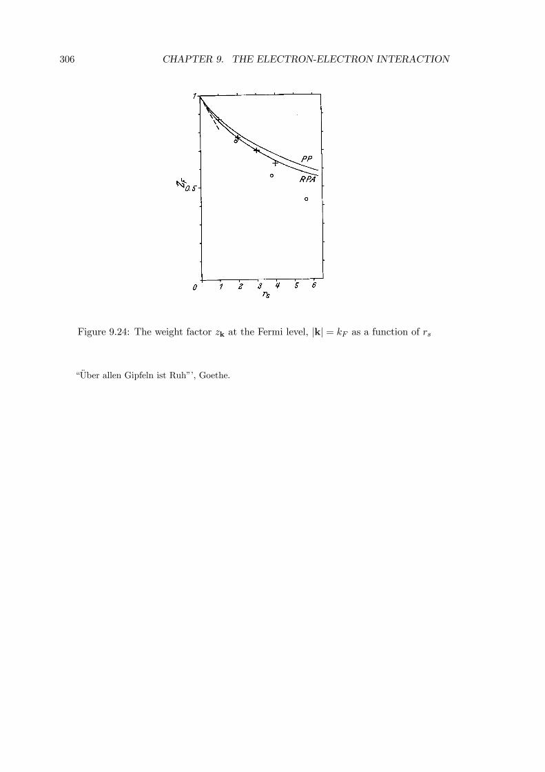
306 CHAPTER 9. THE ELECTRON-ELECTRON INTERACTION
Figure 9.24: The weight factor zk at the Fermi level, |k| = kF as a function of rs
“Uber allen Gipfeln ist Ruh”’, Goethe.


