Diagnosing Unobserved Components inSelf-Adaptive Systems

Paulo CasanovaCarnegie Mellon University

Pittsburgh, PA, USApaulo.casanova@cs.cmu.edu

David GarlanCarnegie Mellon University

Pittsburgh, PA, USAgarlan@cs.cmu.edu

Bradley SchmerlCarnegie Mellon University

Pittsburgh, PA, USAschmerl@cs.cmu.edu

Rui AbreuUniversidade do Porto

Porto, Portugalrui@computer.org

ABSTRACTAvailability is an increasingly important quality for today’ssoftware-based systems and it has been successfully addressedby the use of closed-loop control systems in self-adaptive sys-tems. Probes are inserted into a running system to obtaininformation and the information is fed to a controller that,through provided interfaces, acts on the system to alter itsbehavior. When a failure is detected, pinpointing the sourceof the failure is a critical step for a repair action. However,information obtained from a running system is commonlyincomplete due to probing costs or unavailability of probes.In this paper we address the problem of fault localizationin the presence of incomplete system monitoring. We maynot be able to directly observe a component but we may beable to infer its health state. We provide formal criteria todetermine when health states of unobservable componentscan be inferred and establish formal theoretical bounds foraccuracy when using any spectrum-based fault localizationalgorithm.

Categories and Subject DescriptorsD.2.5 [Testing and Debugging]: Diagnostic aids,Monitors;D.2.4 [Software]: Program Verification—Reliability,Correctnessproofs

General TermsAlgorithms, Reliability, Theory

KeywordsSelf-adaptive systems; Diagnostics; Monitoring.

1. INTRODUCTION

Permission to make digital or hard copies of all or part of this work forpersonal or classroom use is granted without fee provided that copies arenot made or distributed for profit or commercial advantage and that copiesbear this notice and the full citation on the first page. To copy otherwise, torepublish, to post on servers or to redistribute to lists, requires prior specificpermission and/or a fee.Copyright 20XX ACM X-XXXXX-XX-X/XX/XX ...$15.00.

An increasingly important quality for today’s software-based systems is high availability. While high availabilityused to be confined to certain technology outliers (the phonesystem, the electrical grid, etc.) our increasing reliance onsoftware systems has made high availability a requirementfor many systems. This trend has led to an interest in im-proving system resilience by endowing systems with the abil-ity to automatically cope with faults, attacks, changes inresource availability, and shifting system requirements.

One particularly successful approach to improving sys-tem resilience is to adopt a closed loop control paradigm:a system is monitored through a set of “probes” to deter-mine whether the system is working within an appropri-ate behavioral envelope. If not, adaptation mechanismsare selected to improve that behavior, adapting the systemthrough a run-time interface that the system provides [20,23, 31, 32]. Adding such a control loop turns a system intoa self-adaptive system.

Within such a control loop, a critical step is the ability todetect problems and pinpoint their source – sometimes re-ferred to as fault detection and localization. Fault detectionand localization is in general a hard problem for a varietyof reasons. First, there may be many logical explanationsfor an observed problem. Second, faults may be intermit-tent or occur only under certain specific circumstances (suchas when two particular components are communicating).Third, algorithms for localizing faults must find the rightbalance between speed of diagnosis and accuracy, qualitiesthat are often in conflict. Fourth, the information availableto the control layer through probing mechanisms may beincomplete. Prior research by the authors and others hasshown how to address the first three problems [9, 7, 26, 27,28]. However, the third remains an open area.

Incompleteness in monitoring information is particularlyproblematic and, unfortunately, arises commonly. It is prob-lematic because if we are observing a particular part of thesystem it may be hard to determine directly whether ob-served problems are caused by elements within that partof the system. It is common because, in general, systemprobes provide only partial coverage of system behavior.Partial coverage arises for two reasons. First, there are typi-cally costs associated with probing, such as degraded systemperformance, increased system complexity, and deploymentcost. Second, parts of the system may be outside our con-trol to monitor. This occurs, for instance, if those parts are

managed by another organization, the available technologydoes not exist to detect what is going on, or monitoring thatpart of the system may adversely affect important qualityattributes.

In this paper we address the problem of fault localizationin the presence of incomplete system monitoring. The keyobservation is that even though we may not be able to di-rectly observe a component of the system, we may be able toindirectly infer its health state through a collection of ob-servations about its behavior in the context of other systemcomponents that we can monitor. Specifically, given someknowledge about the possible system behaviors, we may beable to infer whether a unobservable component was usedor not and infer its health as if it had been observed. Giventhis observation, we provide formal criteria for determiningwhether such inference is possible. We exemplify the usageof our criteria in the context of a well-known algorithm forfault localization, called Barinel [4]. Such formal criteriaestablish:

(1) theoretical maximum bounds for accuracy of diagnosisusing probabilistic reasoning methods,

(2) theoretical minimum bounds for the case of single-faultsystems, and

(3) an algorithm that computes the maximum possible ac-curacy of fault localization on a system.

Having the ability to determine formally when indirectobservation is adequate to localize faults is an important ca-pability. First, it allows us to reason about the quality ofour monitoring infrastructure with respect to its abilities todetermine problems. Second, it extends the reach of faultlocalization algorithms showing how we can use inferenceto localize faults even in the absence of direct observation.Third, when it is not possible to make such inferences, ithelps provide a basis for deciding whether (and where) todynamically adapt the probing infrastructure (through dy-namic probe placement) to focus on “hidden” parts of thesystem if we suspect that problems are occurring in thatregion.

The rest of the paper is structured as follows: In Section 2we present an example which we will use throughout the pa-per to illustrate fault localization and how our results apply.In Section 3 we present the general principles of spectrum-based fault localization and in Section 4 we present our re-sults. Section 5 shows our algorithm working together with aspecific fault localization algorithm and in Section 6 we showhow probe placement affects diagnosis, going through an ex-ample with several possible probe placements and checkingthe accuracy of each one. Finally, we present related work inSection 7 and the conclusions and future work in Section 8.

2. MOTIVATIONIn this section, we provide an example which we use through-

out the paper to illustrate the application of our techniques.The system is a simulator of a semiconductor manufactur-ing control system used by Samsung Electronics,1 built ac-cording to the specifications provided by Samsung Electron-ics. [8] In a semiconductor factory, semiconductors are man-ufactured in lots that go through several hundreds of pro-cessing stages before they can be shipped or integrated in1http://www.samsung.com/

Event Bus

FT ADS TC.1 TC.2

MOS ADSDB

MOSDB

Figure 1: A partial view of an industrial semicon-ductor manufactoring control system.

other products. The simulated system’s responsibility is totrack the semiconductor lots through the various processingstages, deciding on which pieces of equipment to use andwhen. It effectively runs the factory.

The architecture of the system in illustrated in Figure 1.The system contains an event bus, which mediates the in-teraction of several components that control the productionof semiconductors in Samsung’s fabrication factories.

There are 7 components in this system and one eventbus. The Manufacturing Operating System [MOS] controlsthe manufacturing process, keeping information about thelots produced, including the processing stage of each one.The MOS is connected to the event bus through a Fault-Tolerance mechanism [FT]. Several other instances of theMOS are connected to the event bus and FT provides fail-over capabilities. Because we will not be considering MOSfaults that can be transparently handled by the FT, theother instances are not present in the diagram. The MOSstores its information in a database, the MOSDB, whichmust run at high throughput rates in order to keep up withthe volume of thousands of requests per second.

When a product lot needs to go through another stage ofprocessing, several pieces of equipment may be available toperform the task. The Automatic Dispatch System [ADS]keeps track of the equipment schedule and decides whichone is best suited to perform the task. The ADS keepsits information in another high performance database, theADSDB. Tool Controllers (TC) connect to the physical fac-tory equipment themselves. There are two such controllersin this example.

The actual system at Samsung Electronics is, of course,much larger with many more component instances, but, asthey do not fundamentally change the paradigm of fault-related issues, it is sufficient to work with a simplified versionof the system. (For more details on this system and ourapproach to fault localization, including scalability results,see [8].)

The components in Figure 1 communicate with each otherby exchanging events through an event bus. There are twoimportant interactions that occur when a lot is processedby a piece of equipment: a track-in [TKIN], generated whenthe lot is about to be processed; and a track-out [TKOUT],when a lot exits a piece equipment after processing. TKINand TKOUT are complex computations performed by thefactory systems. For simplicity, we consider here a smallbut representative subset of the computations involved in a

Table 1: Computations performed by the system.Name Components DescriptionC1: MOS request dispatch MOS, ADS, ADSDB The MOS requests equipment from the ADS to process

a lot.C2: ADS process query ADS, ADSDB The ADS computes the best piece of equipment to pro-

cess a lot.C3: MOS update dispatch FT, MOS, MOSDB The MOS receives information about the best equipment

and updates routing information.C4: MOS TC update MOS, MOSDB, TC.1, TC.2 The MOS informs the factory equipment to prepare to

receive the lot.C5: MOS reschedule MOS, MOSDB, ADS,

ADSDBThe MOS needs to reschedule a lot and queries the ADSfor confirmation.

TKIN. Table 1 contains a description of the computations.In this system, we are allowed to probe all components

except the databases. Due to the high volume of data pro-cessed, the databases are often the bottleneck and Samsungis wary of the potential overhead that probing them mightincur. So, both MOSDB and ADSDB are not observable.

With the system in Figure 1 and the list of computationsin Table 1 we can see that some failure patterns can uniquelyidentify faulty components and some cannot. For example, ifonly C3 fails, the faulty component has to be FT (because ifMOS or MOSDB were faulty, C4 would also fail). However,if only C4 fails, we cannot tell whether it was TC.1 or TC.2.Interestingly, if we rule out multiple failures, if both C3 andC4 fail then the fault has to be located in MOSDB, an un-observable component. In the next section we will discuss aformal model that allows us to determine which componentscan and cannot be diagnosed as faulty upon observation.

3. FAULT LOCALIZATIONIn this paper we address the problem of fault localization

when we have incomplete system monitoring. Previous workon fault localization assumes that information is complete.We build upon work in spectrum-based fault localization(SFL), which adopts a reasoning-based approach to fault lo-calization founded on probability theory. The main princi-ples underlying the technique rely on model-based diagnosis(MBD) [15, 17, 18, 25, 34, 21], which uses logical reasoningto find faults and rank them using statistical techniques.

The key insight of spectrum-based fault localization isthat we can infer which components of a system are faultyby examining the components that participated in compu-tations together with a judgement of whether the compu-tations succeeded or failed. The list of components thatparticipated in a computation is termed a spectrum.

In traditional SFL, a component is a program element(e.g., functions, classes, statements) and the computationsare test cases. A suite of test cases is run with the codeinstrumented to keep track of which components were ex-ercised by each test case. The resulting spectra, togetherwith the success/failure output of the test case, is fed intoan algorithm that computes and ranks fault candidates. Afault candidate is a set of components that, if all are faulty,could explain the observed failures. Several algorithms havebeen proposed, which differ in how they compute the faultcandidates and how they rank them. Two examples areTarantula [22] or Barinel [4].

Though SFL has mostly been used with test cases andprogram elements, more recently we have successfully used

Table 2: Spectra in the example system (unobserv-able components are placed in parenthesis).

Computation FT

MOS

(MOSDB)

ADS

(ADSDB)

TC.1

TC.2

C1 - X (-) X (X) - -C2 - - (-) X (X) - -C3 X X (X) - (-) - -C4 - X (X) - (-) X XC5 - X (X) X (X) - -

these algorithms at run time [9]. Here, the components arearchitectural elements of the system and the computationsare the observed behaviors in a system that are classified byan oracle producing spectra and a success evaluations justlike in the traditional case.

A Formal Model for SFLFormally discussing diagnosis and accuracy requires havinga formal model of the system and what is meant by faultybehavior. In this section we introduce a formal probabilisticmodel of a system used by spectrum-based fault localizationalgorithms, which we build on in subsequent sections.

Let σ be a system comprising several components that,interacting with each other, perform computations. In ourexample, σ is the system described in Figure 1. Let compsσbe the non-empty set of all components in system σ. In ourexample, our components are the 7 components: FT, MOS,MOSDB, ADS, ADSDB, TC.1 and TC.2.

Each computation that the system can perform, c, is drawnfrom (2compsσ \ {∅}) × {>,⊥}: the first element in the pairis the non-empty set of components that contributed to thecomputation and the second element is either true (>) orfalse (⊥) depending on whether the computation succeededor failed, respectively. We refer to the first element as thespectrum of the computation (spec(c)) and to the second ele-ment as the failure evaluation of the computation (feval(c)).

A system σ can only produce spectra from a predefinedset, allσ ⊆ (2compsσ \{∅}). This arises from the structure andfunction of the system. For example, in Figure 1, ADSDBcannot communicate directly with MOSDB, and so a spec-trum containing only these components is not possible. Ta-ble 2 contains the spectra that the sample system given inSection 2 can generate.

A behavior of a system defines the probability of a spec-trum being generated. If B is a behavior of system σ, thenB is a random variable drawing values from allσ. To simplify

our notation, we call pB (s) = P(B = s).

4. THE ACCURACY THEOREMSIn this section, we extend the model in Section 3 and

show how diagnosis accuracy can be computed given thatonly some components are observable.

Diagnosis accuracy is defined as a partition of the systemcomponents into groups that have two characteristics:

• If two components are in the same partition, then afault in one of them is indistinguishable from a faultin the other. This means an SFL algorithm will not beable to tell the difference between their health. This isthe theoretical maximum bound for diagnosis accuracy.

• If two components are not in the same partition, thena fault in one of them is distinguishable from a faultin the other. This means an SFL algorithm will beable to tell the difference between their health. This isthe theoretical minimum bound for diagnosis accuracy.The minimum bound guarantee only holds for single-fault systems as multiple faults in several componentsacross different groups may be indistinguishable froma failure in a single group.

Computing the diagnosis accuracy enables reasoning aboutwhether there are enough probes in the system, whether theyare in the right place, and whether enough behaviors havebeen observed for diagnosis.

For example, consider the computations in Table 1. Ifonly C4 fails, we can infer that MOSDB is not faulty despitethe fact that we cannot observe it. Otherwise we would seeC3 and C5 failing too. We know it has to be either TC.1or TC.2. However, because there are no computations inwhich only TC.1 or TC.2 appear, we cannot tell whetherthe problem is in TC.1 or TC.2. In the example in Table 1,the MOSDB is in a different accuracy group from TC.1 andTC.2. TC.1 and TC.2 are in the same accuracy group. Ta-ble 5 contains all accuracy groups of the system in Section 2.

Reasoning about unobservable components requires a pri-ori knowledge of the possible spectra in a system. In theprevious paragraph, our reasoning required us to refer toTable 1 which represents our a priori knowledge in this case.We argue that this a priori knowledge is generally available:System designers know the system’s architecture and whatpaths through the architecture are exercised. Even if somecomponents or connectors cannot be probed, system design-ers know that they exist and what they do. Still, when thisa priori knowledge is unavailable, analysis of accuracy ofthe observable components can still be done, even thoughdiagnosing unobservable components is not possible, as wewill discuss in Section 4.5.

Note that computation of diagnosis accuracy does not it-self compute or rank fault candidates. Such rankings wouldbe handed as a second step, as is typical in SFL, and could behandled by any number of algorithms (some are referencedin Section 7). Indeed, diagnostic accuracy is compatiblewith any spectrum-based fault localization algorithm thatconforms to the model presented in Sections 3, 4.1 and 4.2.

4.1 A Probabilistic Behavior ModelIn system σ, a computation c fails (feval(c) = ⊥) if and

only if any of the components in its spectrum fail. A com-ponent that does not cause the spectrum to fail is a healthy

component. The health of a component is a value in [0, 1]that defines the probability that the component will not failif exercised.

A health state (or state, for short) H of system σ is anassignment of health values, hH (i) to each component i ∈compsσ. The probability of a computation c succeeding isgiven by

∏i∈spec(c) hH (i). (This model assumes that failures

of the components are independent. Handling correlatedfaults can be done by introducing correlation componentsas described in [7].)

For a system σ, behavior B and state H , we define aninstance of the system, Iσ,B,H , which is a random vari-able drawing values from (2compsσ \ {∅}) × {>,⊥}. Theprobability of the system generating a correct computationwith spectrum x is given by P(Iσ,B,H = c ∧ spec(c) =x ∧ feval(c) = >) = pB (x)

∏i∈x hH (i). The probability of

the system generating an incorrect computation with spec-trum x is P(Iσ,B,H = c ∧ spec(c) = x ∧ feval(c) = ⊥) =pB (x)(1−

∏i∈x hH (i)).

These probabilities state how likely are we to observe suc-cesses and failures in different spectra given a set of healthlycomponents, and forms the basis for accuracy: as we willsee later, if two different health states yield the exact sameprobability of success for all possible spectra, then we cannotdistinguish one from the other by observation of the spectra.

4.2 Observability and DistinguishabilityThe previous section presented a general probabilistic be-

havior model for systems. In this section, we will extend themodel to account for the (un)observability of components.

In general, not all components in a system may be ob-servable. In our example, the databases cannot be observed.Unobservability can happen, as described in Section 1, fora variety of reasons. However, these components may stillfail and we want to be able to pinpoint them as the sourceof a failure in such cases. If we do not account for failuresin unobservable components, we may diagnose the incorrectcomponents, triggering incorrect repair actions.

To compensate for the lack of observability of some com-ponents, we need to have some information about when suchcomponents can potentially be used. This is less informa-tion than observing the components directly. For example,computations C1 and C5 in Table 2 use the same visiblecomponents. In either case we only know that the MOSand ADS were involved in the computation. So, if we ob-serve a computation using the MOS and ADS and neitherthe FT, TC.1 or TC.2, we know that ADSDB was involvedand maybe MOSDB was involved, depending on whether weare observing C1 or C5.

To account for unobservability, we divide the componentsof a system σ into two groups, the group of observable com-ponents, obsσ, and the group of unobservable components,nobsσ. This division must form a partition of compsσ: thetwo sets are disjoint (obsσ∩nobsσ = ∅), and complete (obsσ∪nobsσ = compsσ).

We assume there are no spectra in which only unobserv-able components take part as SFL algorithms assume thereare no empty spectra in the system and, therefore, there isno reason to handle this degenerate case.

For each spectrum x of system σ, we define its projectedspectrum, x ′, which is the subset of x that contains onlyobservable components: x ′ = x ∩ obsσ. The projected spec-trum x ′ is what we observe when x happens in the system.

Table 3: Projected spectra corresponding to the ex-ample of Table 2.

Projected FT MOS ADS TC.1 TC.2P1 (C1,C5) - X X - -P2 (C2) - - X - -P3 (C3) X X - - -P4 (C4) - X - X X

Table 3 contains the projected spectra corresponding to theexample in Table 2.

Because projected spectra are subsets of the spectra, itmay happen that two spectra, x1, x2 ∈ allσ are such thatx1 6= x2 ∧ x ′1 = x ′2. In this case, we say that spectra x1 andx2 are indistinguishable. What we observe when x1 happensis the same as when x2 happens. Given a projected spectray ′, we define the reverse projection of y ′, revσ(y ′), the setof spectra x such that x ∈ allσ and x ′ = y ′. Naturally,x ∈ revσ(x ′). In our example, the projected spectra of bothC1 and C5 is P1. The reverse projection of P1 is C1 andC5. The reverse projection tells us which spectra could havebeen responsible for the observation.

Given a system instance Iσ,B,H , the probability that weobserve a projected spectra y ′ and a failure evaluation of> isgiven by hH (y) =

∑x∈revσ(y′) pB (x)

∏i∈x hH (i). This equa-

tion just states that the probability of observing a successfulprojected spectra y ′ is to observe any successful spectra xsuch that x ′ = y ′.

We define the set of all projected spectra of a system σ,allprojσ, as the set with the projections of all spectra inallσ. allprojσ =

⋃x∈allσ x ′. The projected spectra define the

observable behavior of the system. The probability of a pro-jected spectra y ′ being observed is pB (y ′) =

∑x∈revσ(y′) pB (x).

Two systems, σ with behavior Bσ and state Hσ, and φ,with behavior Bφ and state Hφ, such that (1) allprojσ =allprojφ, (2) ∀ y ′ : allprojσ • pBσ (y ′) = pBφ(y ′) and (3)

∀ y ′ : allprojσ • hHσ (y ′) = hHφ(y ′), are indistinguishable byobservation.

If two systems σ and φ are indistinguishable by obser-vation then, without any additional information other thanobservation of projected spectra, it is not possible to knowwhether observations are being produced by σ or φ as theywill generate the same observations with the same probabil-ity distribution.

4.3 The Accuracy GroupsFor a component i of a system σ, we define its partici-

pating projection, partprojσ(i) as being the set of projectedspectra of σ that contain in its reverse projection at leastone spectra containing i . The participating projection of acomponent is the set of all projected spectra that the com-ponent may influence. If the component i is observable, thenthe projected spectra is the set of all computations in whichi is involved. Observing one of those spectra implies i wasused. For example, P1 is in the participating projection ofthe MOS; the MOS was used if we observe P1.

However, if the component is not observable, then observ-ing one of the spectra in partprojσ(i) means component imay have been used in the computation. We may not beable to tell for sure as there may be computations x1 and x2such that i participates in x1 but not x2 and x ′1 = x ′2. For ex-ample, P1 is in the participating projection of the MOSDB;the MOSDB may have been used if we observe P1. How-ever, P2 is not in its participating projection so observing P2

Table 4: Participating projection of all componentsin the example of tables 2 and 3.

Component Participating projectionFT P3MOS P1, P3, P4ADS P1, P2MOSDB P1, P3, P4ADSDB P1, P2TC.1 P4TC.2 P4

Table 5: Accuracy groups corresponding to the com-ponents in 4.

Group Participating projectionFT P3MOS, MOSDB P1, P3, P4ADS, ADSDB P1, P2TC.1, TC.2 P4

means the MOSDB was not used. Table 4 contains the par-ticipating projections of the system whose projected spectraare in Table 3.

For a system σ, we define its accuracy partition, accσ, asa partition of all components in compsσ (including those innobsσ) into accuracy groups. Two components i and j be-long to the same accuracy group if and only if they have thesame partipating projection. Two components belong to thesame accuracy group if and only if their health can influencethe exact same set of visible behaviors. Table 5 contains theaccuracy groups corresponding to the participating projec-tions of Table 4.

4.4 The Accuracy TheoremsTo prove the claims about the theoretical maximum and

minimum bounds of accuracy we need to prove some pre-liminary results. First we show through Theorem 1 that theprobability of projected spectra being observed can alwaysbe computed. Then we show through Theorem 2 that it isnot possible to compute the relative probability of undistin-guishable spectra.

Then we prove the theorems that establish the maximumbounds for diagnosis accuracy: the Strong Accuarcy Theo-rem, Theorem 3, and the Weak Accuracy Theorem, Theo-rem 4. The former is more restrictive than the latter but thelatter is universally applicable. The last theorem presented,Theorem 5 provides the minimum bounds for diagnosis ac-curacy.

4.4.1 Initial Theorems

Theorem 1. Let Iσ,B,H be an instance of a known sys-tem σ with an unknown behavior B and unknown health H .Observation of the system allows eventually determining thevalue of pB (y ′) (with an arbitrary low error margin) for allprojected spectra y ′.

This theorem states that by observing a system, even-tually we will determine the probabilities with which eachprojected spectra will occur.

Proof. Since, by definition, all projected spectra are dis-tinguishable by observation and pB (y ′) is the probability

that y ′ is generated, then, by the law of large numbers, thestatistical observation of outcomes of the projected spectrawill converge to their probabilities.

Theorem 2. Let Iσ,B,H be an instance of a known systemσ with unknown behavior B and unknown health H . Obser-vation of the system does not allow determining pB (x | x ′)where x is a spectra except when there is only x whose pro-jected spectra is x ′.

This theorem states that just by observing a system wecannot determine the probabilities of the original spectraocurring . We will, by Theorem 1, know the probabilitiesthat projected spectra will occur, but will not be able to knowhow these probabilities decompose in the different spectrathat comprise revσ(y ′).

Proof. If x1 6= x2 ∧ y = x ′1 = x ′2, then pB (y) = pB (x1) +pB (x2) (assuming x1 and x2 are the only spectra that projectto y – extending this to several xi is trivial). Therefore, anycombination of values of the probabilities of x1 and x2 thatsum to the same value will yield the same observations.

Because pB (x1) = pB (x1 | y)pB (y), we know that pB (x1 |y) + pB (x2 | y) = 1. However, because x1 and x2 are in-distinguishable by observation, all distributions of 1 overpB (xi | y) will yield the same result and are, therefore, in-distinguishable.

4.4.2 The Strong Accuracy Theorem

Theorem 3 (Strong Accuracy Theorem). Let aninstance of a known system σ in an unknown state H1 beIσ,B,H1 . Let i and j be two observable components of σsuch that i and j belong to the same accuracy group andhH1(i) 6= hH1(j ). Then, the instance Iσ,B,H2 where H2 is thesame as H1 except that the healths of i and j are reversed,is indistinguishable from observation from Iσ,B,H1 .

Theorem 3 states an important and intuitive result: if twocomponents are always used together, we can never distin-guish the health of one from the health of the other. Thismeans trying to rank the two components as fault candi-dates is useless as any distibution of blame for the failuresamong them is arbitrary. An example of this is presented inSection 6 where we show how these results can be used toreduce the search space for fault candidates.

Proof. The probability that a certain projected spectray ′ succeeds in Iσ,B1,H1 , S(y ′), is given by:

S(y ′) =∑

x∈revσ(y′) pB1(x)∏

i∈x hH1(i)

= pB1(y ′)∑

x∈revσ(y′) pB1(x | y ′)∏

i∈x hH1(i)(1)

Because all observable components appear in all spectrathat project to the same projected spectra, the previousequation can be rewritten as:

S(y ′) = Ao ×An , whereAo = pB1(y ′)

∏i∈y hH1(i)

An =∑

x∈revσ(y′) pB1(x | y ′)∏

i∈x\y′ hH1(i)

If i and j are both observable then their health will ap-pear in Ao and not in An . Because Ao ∝ hH1(i)hH1(j ),the success probability of each spectra is the same in bothcases.

4.4.3 The Weak Accuracy Theorem

Theorem 4 (Weak Accuracy Theorem). Let σ bea system with components i and j in the same accuracygroup. Let H1 and H2 be two states of the system suchthat hH1(k) = hH2(k) for all components k /∈ {i , j}. LethH1(i) 6= hH1(j ) and let the health of components i and jbe reversed in H2. Then, for every behavior B1, there is atleast one behavior B2 such that Iσ,B1,H1 is indistinguishableby observation from Iσ,B2,H2 .

Theorem 4 states that a system with observations thathave components i and j in the same accuracy group, regard-less of whether the compoenents are observable or not, is in-distinguishable from a system in which the healths of i and jare reversed. This theorem states that, associated with eachhealth state, there may be different behavior (B2 6= B1).However, the observable behavior is not changed, otherwisethe systems would not be indistinguishable. Because this isa weaker condition that the one in Theorem 3, which saysthat the behavior for both health states may be exactly thesame, this theorem is named “weak”.

Proof. This theorem essentially states that, for everyB1, there is a B2 such that, for all y ′ ∈ allprojσ, Equation 1holds.

For all y ′ ∈ allprojσ, pB1(y ′) = pB2(y ′) otherwise, byTheorem 1 the behaviors would be distinguishable. Thisleaves choosing a B2 such that

∑x∈revσ(y′) pB2(x | y ′)

∏k∈x\y′ hH2(k)

=∑

x∈revσ(y′) pB1(x | y ′)∏

k∈x\y′ hH1(k)(2)

For notation simplicity, let hi = hH1(i) = hH2(j ) and hj =hH1(j ) = hH2(i). It is important to note that either bothcomponents i and j appear in Equation 2 or none appear.Otherwise they would not be in the same accuracy group.Equation 2 can be rewritten as:

α2C + β2Dhi + γ2Ehj + δ2Fhihj

= α1C + β1Dhi + γ1Ehj + δ1Fhihj(3)

The terms C , D , E , and F depend only on the healths inH1 and H2 but not on hi nor on hj so they are equal in bothsides. The terms αk , βk , γk and δk depend only on B1 andB2. By Theorem 2, as long as the values in α2, β2, γ2 andδ2 add up to 1, we can choose whatever values we want asit will not affect the visible behavior.

Because αk +βk +γk +δk = 1, we can see these as weightsfor the other terms. We can choose α2 = α1 and δ2 = δ1eliminating these terms from the equation. The remainingequation is:

β2Dhj + γ2Ehi = β1Dhi + γ1Ehj

In this equation, β1 and γ1 are fixed (they are determinedby B1) and we need to find out if there is a β2 and a γ2 (thatdefine B2) that can solve this equation. It may happen thateither D or E (or both) are zero but in either case solvingthe equation is trivial.

Because β2 and γ2 are weighting Dhj and Ehi , this equa-tion has no solution if and only if Dhj < β1Dhi + γ1Ehj andif Ehi < β1Dhi + γ1Ehj . Solving these two inequations forhi and hj yields:

hj <β1

1−γ1 ED

hi

hi <γ1

1−β1 DE

hj

Replacing hi on the top equation yields hj <β1

1−γ1 ED

γ11−β1 D

E

hj .

With some algebraic manipulation this leads to 1 + β1DE

+

γ1ED< 0 which is impossible as β1, γ1, D and E are all

drawn from [0, 1].This means that there is always a β2 and γ2 that make

the equation β1Dhi + γ1Ehj = β2Dhj + γ2Ehi true, provingthe theorem.

4.4.4 Minimum Accuracy TheoremA single fault state of a system is a state in which a single

component, either observable or not, has health < 1.

Theorem 5 (Minimum Accuracy Theorem). Let σbe a system, B1 its behavior and H1 its single fault state.Let i be the faulty component. If component i is used in B1,then let H2 be an arbitrary single-fault state such that thereis a B2 that makes Iσ,B1,H1 indistinguishable from Iσ,B2,H2 .H2 will have a single fault in the same accuracy group.

The minimum accuracy theorem, Theorem 5, states thatwe can always identify the accuracy group that contains thefaulty component in a single fault state. It states that anytwo single-fault states that generate the same observablebehavior will necessarily have faults in the same accuracygroup. Together with the weak accuracy theorem, Theo-rem 4, it states that in a single fault system, it is always andonly possible to identify the accuracy group of the compo-nent that has failed.

Proof. Let H2 be a single fault state with faulty compo-nent j which is not in the same accuracy group of i .

Because i and j are not in the same accuracy group, thenpartprojσ(i) 6= partprojσ(j ), otherwise they would be in thesame accuracy group. Then there exists either a spectrumin partprojσ(i) which does not exist in partprojσ(j ) or theother way around. Lets consider both cases separately.

• If there is a projected spectrum y ∈ partprojσ(i) suchthat y /∈ partprojσ(j ), then pB1(y) > 0, meaining thateventually a spectrum y is observed with a failure eval-uation ⊥. Since y /∈ partprojσ(j ), then this behaviorcannot be reproduced with a single fault in j .

• If there is a projected spectrum y ∈ partprojσ(j ) suchthat y /∈ partprojσ(i), then pB2(y) > 0. This meansthat, in the single fault scenario with H2, y will even-tually be observed with a failure evaluation of ⊥ whichcannot be reproduced with a single fault in i .

4.5 A Priori and A Posteriori AnalysesAccuracy analysis, as described so far, uses a priori knowl-

edge of the system to determine accuracy groups. If thisknowledge does not exist, it is not possible to pinpoint non-observable components because we have no information aboutthem.

However, the strong accuracy theorem (Theorem 3) andthe minimum accuracy theorem (Theorem 5) are still usefulas they may significantly reduce the search space for solu-tions.

Without a model of allσ, the accuracy groups cannot becomputed. However, the law of large numbers guaranteesthat, as the number of observations increase, our estimatesof pB (y) converge to the actual values and we will eventuallyidentify all possible projected spectra.

This means that, a posteriori we can compute the accu-racy groups using an estimate of allσ, which is the set ofobserved projected spectra. For example, even if the data inTable 1 were unavailable, we would observe the MOS beingused with the ADS performing computations, the ADS byitself, the FT with the MOS and the MOS with TC.1 andTC.2, effectively allowing us to reconstruct Table 3. Natu-rally we would not be able to observe MOSDB and ADSDBand, consequently, Table 1 is not reconstructable from ob-servation. Hence the limitation the a posteriori analysis.

4.6 Implementation AlgorithmThe computations described in the previous sections lead

to an algorithm that computes the accuracy groups of a sys-tem σ given its spectra, allσ, and the list of observable (obsσ)and non-observable (nobsσ) components. The pizzicato al-gorithm presented below performs the same computationswe’ve done in the previous sections. It first computes PP ,the participating projections. This corresponds to what wasdone in Table 4. The transformation done for Table 3 isperformed implicitly. Then it computes AG, the accuracygroups, corresponding to what was done in Table 5.

function pizzicato(allσ, obsσ, nobsσ)PP ← ∅for all s ∈ allσ do

s ′ = s ∩ obsσfor all i ∈ s do

if ¬(∃(a, b) : PP | a = i) thenPP(i)← ∅

end ifPP(i)← PP(i) ∪ {s ′}

end forend forAGt ← ∅for all (i , pp) ∈ PP do

if ¬(∃(a, b) : AGt | a = pp thenAG1(pp) = ∅

end ifAGt(pp)← AGt(pp) ∪ {i}

end forAG ← ∅for all (pp, ag) ∈ AGt do

AG ← agend forreturn AG

end function

The pizzicato algorithm has linear complexity in the num-ber of components and the number of spectra. Its complex-ity is O(M × N ) where M = #compsσ and N = #allσmaking it a fast-performing algorithm even for very largesystems.

5. RELEVANCE FOR FAULT LOCALIZA-TION

The accuracy theorems, described above, establish accu-racy limits on fault localization. However, they do not definehow to perform localization.

Table 6: Example spectraFT MOS ADS TC.1 TC.2 R1 R2- X X - - > ⊥- - X - - > >- - X - - > >- - X - - > >X X - - - > >- X - X X ⊥ >- X - X X > >

Table 7: Results of running example of Table 6through Barinel [4] without pizzicato preprocessing

.

Scenario Candidate RankR1 TC.1 ≈ 41%R1 TC.2 ≈ 41%R1 MOS ≈ 17%R2 MOS 50%R2 ADS 50%

Several algorithms exist that perform statistical fault lo-calization, e.g., Tarantula [22] or Barinel [4]. We argue thatthe results presented in Section 4, plus the pizzicato algo-rithm defined in Section 4.6, complement existing fault lo-calization algorithms by: (1) reducing the size of the searchspace for faults and increasing the accuracy of the outputand (2) allowing a priori detection of indistinguishable faults,enabling decisions on probe placement and test generation.In the following sections, we explore these two enhance-ments.

5.1 Reducing Search Space and IncreasingAccuracy

The first enhancement is the reduction of the search spaceby removing indistinguishable components. This is done byreplacing spectra of components with spectra of accuracygroups before fault localization. Because several fault local-ization algorithms do not perform this analysis, they have toprocess larger sets and produce worse outputs. As shown byTheorem 4, it is not possible to pinpoint specific componentsin accuracy groups so either fault localization algorithms willnot pinpoint the correct components or they will with lessconfidence.

Consider, for example, the set of spectra in Table 6 (onlyobservable components considered) which could be observedfrom the system described in Section 2. Results in col-umn R1 were obtained when TC.1 is non-healthy and re-sults in column R2 were obtained when MOS was unhealthy.Both runs are single-fault scenarios which we ran throughBarinel [4], an algorithm which is optimal for this case (seelater in this section for some more information on Barinel).Table 7 contains the results when running Barinel directlyon the data in Table 6 and Table 8 contains the results whenrunning Barinel after processing Table 6 through pizzicato.

These results illustrate that, in this case, with pizzicatopreprocessing, the confidence on the first scenario is much

Table 8: Results of running example of Table 6through Barinel [4] with pizzicato preprocessing

.

Scenario Candidate RankR1 (TC.1,TC.2) ≈ 71%R1 MOS ≈ 29%R2 MOS 50%R2 ADS 50%

greater because there are fewer components to “split” therank. In fact, if the number of samples is increased, theconfidence without pizzicato preprocessing will stabilize as-signing blame to TC.1 and TC.2 at 50%/50%, while withpizzicato it will increase to 100%.

The second scenario illustrates this in comparison with theprevious scenario. Here we also have a 50%/50% split butthis is due to the lack of observations. Since the only scenariowe have a failure in is the first, in which both MOS and ADSwere used together, both have the same probability.

Essentially, preprocessing the output with pizzicato allowsthe diagnostic system to distinguish when more informationwill eventually pinpoint the source of failure (Scenario 2) orwhen it is not useful to wait for more information as failuresare indistinguishable. This is especially useful when using ameasure such as entropy [30] to decide whether to observemore spectra or produce a diagnosis based on the currentset of spectra, as we have shown in [7].

Some Details on BarinelBarinel is described in more detail in [2]. Here we providesome basic description of the algorithm so that the values inTable 7 and Table 8 can be more easily understood.

Let D denote a set of fault candidates expressing a diag-nosis. For instance, D = 〈{c1, c3, c4}〉 indicates that com-ponents c1, c3, and c4 are simultaneously at fault, and noother. Barinel sorts the faulty candidates in D by the prob-ability that each candidate explains the fault. As with mostspectrum-based reasoning, it is comprised of two phases:candidate generation and candidate ranking.

The problem of finding fault candidates can be definedin terms of the widely-known minimal hitting set (MHS)problem [15]. The precise computation of MHS is highlydemanding [19], restricting its direct usage for diagnosis.However, in practice, previous research has found that pre-cise computation of D is not necessary [1]. Staccato is alow-cost heuristic for computing a relevant set of multiple-fault candidates.

Candidate Ranking.The candidate generation phase may result in an exten-

sive list of diagnosis candidates. As not all candidates havethe same probability of being the true fault explanation,techniques have been devised to assign a probability to eachdiagnosis candidate dk . Each candidate dk is a subset ofthe system components that, when at fault, can explain thefaulty behavior. The probability of a diagnosis candidate be-ing the true fault explanation, Pr(dk | obs), given a numberof observations obs, is computed using Bayesian probabilityupdates. An observation obs is a tuple (ai∗, ei).

Executing each test case ti from the test suite T , theprobability of each candidate is updated following Bayes’rule

Pr(dk | obs) = Pr(dk ) ·∏

obsi∈obs

Pr(obsi | dk )

Pr(obsi)

Pr(dk ) is the a priori probability of the candidate (i.e., theprobability before any test is executed), defined as Pr(dk ) =

p|dk | · (1 − p)M−|dk | where p is the a priori probability of acomponent being faulty. The prior probability given no ob-servations is an approximation to 1 fault for every 1000LOC,1/1000 = 0.001 [6].

Pr(obsi | dk ) represents the conditional probability of theobserved outcome ei produced by a test ti (obsi), assumingthat candidate dk is the actual diagnosis

Pr(obsi | dk ) =

0 if ei ∧ dk are inconsistent;

1 if ei is unique to dk ;

ε otherwise.

where ε is defined as

ε =

∏

j∈dk∧aij=1

hj if ei = 0

1−∏

j∈dk∧aij=1

hj if ei = 1

and aij represents the coverage of the component j whenthe test i is executed. As this information is typically notavailable, the values for hj ∈ [0, 1] are determined by max-imizing Pr(obs | dk ) using maximum likelihood estimation.To solve the maximization problem, a simple gradient ascentprocedure [5] (bounded within the domain 0 < hj < 1) isapplied.

Pr(obsi) represents the probability of the observed out-come, independently of which diagnostic explanation is thecorrect one and thus needs not be computed directly. Thevalue of Pr(obsi) is a normalizing factor given by Pr(obsi) =∑

dk∈DPr(obsi | dk ) · Pr(dk ).

The Barinel algorithm is used to compute the probabili-ties of each diagnosis candidate dk .

5.2 Enabling Probe Placement and Test Gen-eration

When using the accuracy analysis we can detect whichcomponents are indistinguishable. This indistinguishabilitymay not be fundamental: it may only be due to lack ofprobing. In the example of Section 2, components TC.1 andTC.2 are indistinguishable because they are both invokedfrom the MOS in the same computation.

However, placing additional probes may allow splittingthe communication with TC.1 and TC.2, effectively splittingthe spectrum in two: one with MOS and TC.1 and anotherwith MOS and TC.2.

This decision can be made before the system is run ordynamically. At run time, as part of a self-adaptive system,it is possible to decide not to place the probes in the busconnections (as this will slow the system down) and acceptthe inaccurate diagnosis. However, after a problem has beendiagnosed in the accuracy group, probes could be deployeddynamically to obtain a more accurate diagnosis.

6. APPLICATION EXAMPLEIn the previous sections we presented theoretical results

on diagnosis accuracy and exemplified them on the systempresented in Section 2. In this section we present a sec-ond example, based on a different computation paradigm,in order to illustrate how observability affects diagnosis ac-curacy. We chose a simple, well-known, example to allow foran intuitive confirmation of the theoretical results obtained.

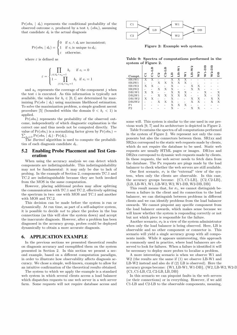
The system to which we apply the example is a standardweb system in which several clients access a load balancerwhich dispatches requests to one web server in a web serverfarm. Some requests will not require database access and

C1

C2

LB

W1

W2

DB

Figure 2: Example web system.

Table 9: Spectra of computations performed in thesystem of Figure 2.

Compt. C1

C1-L

B

C2

C2-L

B

LB

LB-W

1

W1

LB-W

2

W2

W1-D

B

W2-D

B

DB

SR1W1 X X - - X X X - - - - -SR2W1 - - X X X X X - - - - -SR1W2 X X - - X - - X X - - -SR2W2 - - X X X - - X X - - -DR1W1 X X - - X X X - - X - XDR2W1 - - X X X X X - - X - XDR1W2 X X - - X - - X X - X XDR2W2 - - X X X - - X X - X XP1 - - - - X X X - - - - -P2 - - - - X - - X X - - -

some will. This system is similar to the one used in our pre-vious work [9, 7] and its architecture is depicted in Figure 2.

Table 9 contains the spectra of all computations performedin the system of Figure 2. We represent not only the com-ponents but also the connectors between them. SR1xx andSR2xx correspond to the static web requests made by clients,which do not require the database to be used. Static webrequests are usually HTML pages or images. DR1xx andDR2xx correspond to dynamic web requests made by clients.In these requests, the web server needs to fetch data fromthe database. The Px requests are pings made by the loadbalancer to check whether the web servers are still available.

One first scenario, σ1 is the “external” view of the sys-tem, when only the clients are observable. In this case,the accuracy groups become: {C1,C1-LB}, {C2,C2-LB},{LB,LB-W1,W1,LB-W2,W2,W1-DB,W2-DB,DB}

This result means that, for σ1, we cannot distinguish be-tween a failure in the client and its connection to the loadbalancer, we can distinguish between problems in differentclients and we can identify problems from the load balanceronwards. We cannot pinpoint any specific component fromthe load balancer onwards, which makes sense because wewill know whether the system is responding correctly or notbut not which piece is responsible for the failure.

Another scenario, σ2 is a view of the system administratorwhen only the load balancer is being observed. Here, LB isobservable and no other component or connector is. Thisscenario will yield a single accuracy group with all compo-nents inside. While it appears uninteresting, this approachis commonly used in practice, where load balancers are ob-served to look for failures. When a failure is identified it willbe necessary to deploy more probes to localize a problem.

A more interesting scenario is when we observe W1 andW2 (the results are the same if (1) we observe LB-W1 andLB-W2 instead and also do if (2) LB is observed). Here theaccuracy groups become: {W1,LB-W1,W1-DB}, {W2,LB-W2,W2-DB},{C1,C1-LB,C2,C2-LB,LB,DB}

In this scenario we can pinpoint faults in the web servers(or their connections) or in everything. However, if we addC1-LB and C2-LB to the observable components, meaning,

in practical terms, that we probe the input of the load bal-ancer, the accuracy groups become: {C1,C1-LB, }, {C2,C2-LB},{W1,LB-W1,W1-DB}, {W2,LB-W2,W2-DB}, {LB,DB}

In this scenario we can now distinguish failures in clientsand web servers although we cannot tell the difference be-tween failures in the load balancer and the database. Whilethis may seem unintuitive, it is an expected result: a sce-nario in which the load balancer fails half the time is equalto a scenario in which the database always fails and half ofthe requests are dynamic.

One aspect of this example that may appear unclear isthat we always assume that all computations terminate nor-mally, meaning that the load balancer always returns a replyto a request made by a client. Handling non-responsivenessrequires adding new spectra with only the involved compo-nents. For example, to handle non-responsiveness of the loadbalancer would require a computations that include C1,C1-LB and LB and another one that includes C2,C2-LB andLB. Addition of these computations would make the LBidentifiable as a fault in its own failure group because now,if both C1 and C2 have a non-responsive failure from LB,the problem must lay in the common component, LB.

7. RELATED WORKRecent work has already been done in the area related to

diagnosis accuracy. In [24] probe placement and its impacton diagnosis is directly discussed. The concept of ambiguitygroup is introduced (equivalent, more or less to our accu-racy group) and ways to introduce probing are proposed.However, only sequential computations are considered, e.g.,computations in which the components of the group are ex-ercised sequentially. Thus our work generalizes that pro-posed in [24] to any computation model. [10] addresses howto improve SFL accuracy in tightly coupled systems by split-ting components into smaller components, although probingitself is not discussed as all components are assumed to beobservable.

More generally, in the area of self-adaptive systems (SAS),a significant amount of research has been done. Severalmulti-goal optimization frameworks for self-adaptive systemsexist that could benefit from diagnosis accuracy to drive sys-tem adaptation. Rainbow [12, 20] uses software architectureas a backbone for SAS and Zanshin [31] uses goal-orientedrequirements. Several surveys and roadmaps exist that refersome of the many approachs to SAS: [11, 29, 16]. However,none of this work has directly tackled the problem of diag-nosis for unobservable components.

Spectrum-based fault localization, the core algorithms thatpinpoint the accuracy groups at fault, also have a variety ofapproaches, including algorithmic approaches (e.g., [22, 2]),simularity coefficient calculation (e.g., [14] and those listedin [3]), and the use of neural networks [33]. Our work com-plements these approaches by reducing the size of the can-didates that need to be considered by these approaches, andincreasing the accuracy of their output.

Furthermore, diagnosis accuracy enables reasoning aboutdiagnosis uncertainty and has the potential to be used by AIplanners to decide where to place probes. A discussion ofplanning under uncertainty can be found in the CassandraPlanner work [13].

8. CONCLUSIONS AND FUTURE WORK

This paper provides a definition of diagnosis accuracy inthe presence of unobservable components, and an algorithmto compute it. Diagnosis accuracy is defined as a partitionof the system’s components into groups: components in thesame group cannot be individually identified as faulty. Weprovided a theoretical proof that these groups establish amaximum accuracy bound and that they are also the mini-mum accuracy bound in the case of a single-fault scenario.

These results allow a diagnostic system to define whichprobes to have on a system and identify what they are ca-pable of pinpointing in the event of a failure. Further, theyprovide a basis for dynamically controlling probing on a self-adaptive system.

We plan to continue future work to extend these resultsalong three dimensions. First, this work can be used to ex-tend current state of the art for self-adaptive systems byincluding formal reasoning about dynamic probe placementand dynamic testing. Dynamic probe placement controlswhen probes can be placed in a system in order to achievean optimum balance between probing cost and diagnosis ac-curacy. Dynamic testing can be used to produce additionalcomputations and improve diagnosis. For example, if we areunsure whether the MOSDB or the MOS are faulty, we canexplicitly exercise just one of them.

Second, the theoretical results in this paper can be im-proved under some conditions. In the approach taken bythis paper, we have assumed that components are either ob-servable or non-observable, but, especially in the presenceof dynamic probe placement, components may be observ-able at some times but not others. This may also occur ifprobes cannot always deterimine whether a component par-ticipated in a computation. For example, a file system probemay be able to detect when a component was used only ifthe component uses the file system. With the current ap-proach, we need to disregard knowledge of the observationsof these components and consider them as non-observable,throwing away useful information that could help us to pro-vide a more accurate diagnosis. We believe it is possible toextend the theory to consider these sporadic observations.

Third, although in this paper we explored the applicationof diagnosis accuracy in the context of self-adaptive systems,the results presented here are potentially much more generaland may also apply to design time. Design-time code instru-mentation is akin to probe placement at run time and ourapproach would allow (1) determining what needs to be in-strumented, and (2) when there are enough test cases todistingush bugs in different parts of the code. Additionally,pizzicato’s reduction of the search space for faults may im-prove the performance of existing SFL algorithms.

AcknowledgmentsThis work was supported in part by the National ScienceFoundation under Grant CNS 1116848, the Army ResearchOffice under Award No. W911NF-09-1-0273, the Office ofNaval Research under Grant N000141310401 and SamsungElectronics. Furthermore we would like to thank JungsikAhn, of Samsung Electronics, who helped us define the sim-ulator described in Section 2.

9. REFERENCES[1] R. Abreu and A. J. C. van Gemund. A low-cost

approximate minimal hitting set algorithm and its

application to model-based diagnosis. In V. Bulitkoand J. C. Beck, editors, Proceedings of the 8thSymposium on Abstraction, Reformulation andApproximation (SARA’09), Lake Arrowhead,California, USA, 8 – 10 July 2009. AAAI Press.

[2] R. Abreu and A. J. C. van Gemund. Diagnosingmultiple intermittent failures using maximumlikelihood estimation. Artif. Intell.,174(18):1481–1497, 2010.

[3] R. Abreu, P. Zoeteweij, and A. J. C. V. Gemund. AnEvaluation of Similarity Coefficients for Software FaultLocalization. In Pacific Rim International Symposiumon Dependable Computing, pages 39–46, 2006.

[4] R. Abreu, P. Zoeteweij, and A. J. C. v. Gemund.Spectrum-based multiple fault localization. InProceedings of the 2009 IEEE/ACM InternationalConference on Automated Software Engineering, ASE’09, pages 88–99, Washington, DC, USA, 2009. IEEEComputer Society.

[5] M. Avriel. Nonlinear Programming: Analysis andMethods. Dover Books on Computer Science Series.Dover Publications, 2003.

[6] J. Carey, N. Gross, M. Stepanek, and O. Port.Software hell. pages 391–411, 1999.

[7] P. Casanova, D. Garlan, B. Schmerl, and R. Abreu.Diagnosing architectural run-time failures. InProceedings of the 8th International Symposium onSoftware Engineering for Adaptive and Self-ManagingSystems, 20-21 May 2013.

[8] P. Casanova, D. Garlan, B. Schmerl, R. Abreu, andJ. Ahn. Applying autonomic diagnosis at samsungelectronics. Technical Report CMU-ISR-13-111,Carnegie Mellon University, Sep 2013.

[9] P. Casanova, B. R. Schmerl, D. Garlan, and R. Abreu.Architecture-based run-time fault diagnosis. InI. Crnkovic, V. Gruhn, and M. Book, editors, ECSA,volume 6903 of Lecture Notes in Computer Science,pages 261–277. Springer, 2011.

[10] C. Chen, H.-G. Gross, and A. Zaidman. Improvingservice diagnosis through increased monitoringgranularity. In Proceedings of the 7th InternationalConference on Software Security and Reliability(SERE), 18-29 June 2013.

[11] B. H. Cheng et al. In B. H. Cheng, R. Lemos,H. Giese, P. Inverardi, and J. Magee, editors, SoftwareEngineering for Self-Adaptive Systems, chapterSoftware Engineering for Self-Adaptive Systems: AResearch Roadmap, pages 1–26. Springer-Verlag,Berlin, Heidelberg, 2009.

[12] S.-W. Cheng, D. Garlan, and B. Schmerl.Architecture-based self-adaptation in the presence ofmultiple objectives. In Proceedings of the 2006international workshop on Self-adaptation andself-managing systems, SEAMS ’06, pages 2–8, NewYork, NY, USA, 2006. ACM.

[13] G. Collins and L. Pryor. Planning under uncertainty:Some key issues. In Proceedings of the FourteenthInternational Joint Conference on ArtificialIntelligence, pages 1567–1573, 1995.

[14] A. da Silva Meyer, A. A. F. Farcia, and A. P.de Souza. Comparison of similarity coefficients usedfor cluster analysis with dominant markers in maize

(zea mays l). Genetics and Molecular Biology,27(1):83–91, 2004.

[15] J. de Kleer and B. C. Williams. Diagnosing multiplefaults. Artif. Intell., 32(1):97–130, Apr. 1987.

[16] R. de Lemos et al. Software Engineering forSelf-Adaptive Systems: A second Research Roadmap.In R. de Lemos, H. Giese, H. Muller, and M. Shaw,editors, Software Engineering for Self-AdaptiveSystems, number 10431 in Dagstuhl SeminarProceedings, Dagstuhl, Germany, 2011. SchlossDagstuhl - Leibniz-Zentrum fuer Informatik, Germany.

[17] A. Feldman, G. M. Provan, and A. J. C. van Gemund.Computing minimal diagnoses by greedy stochasticsearch. In D. Fox and C. P. Gomes, editors, AAAI,pages 911–918. AAAI Press, 2008.

[18] A. Feldman and A. van Gemund. A two-stephierarchical algorithm for model-based diagnosis. InProceedings of the 21st national conference onArtificial intelligence - Volume 1, AAAI’06, pages827–833. AAAI Press, 2006.

[19] M. R. Garey and D. S. Johnson. Computers andIntractability; A Guide to the Theory ofNP-Completeness. W. H. Freeman & Co., New York,NY, USA, 1990.

[20] D. Garlan, S.-W. Cheng, A.-C. Huang, B. Schmerl,and P. Steenkiste. Rainbow: architecture-basedself-adaptation with reusable infrastructure.Computer, 37(10):46–54, 2004.

[21] A. Gonzalez-Sanchez, E. Piel, H.-G. Gross, and A. vanGemund. Prioritizing tests for software faultlocalization. In Quality Software (QSIC), 2010 10thInternational Conference on, pages 42–51, 2010.

[22] J. A. Jones and M. J. Harrold. Empirical evaluation ofthe Tarantula automatic fault-localization technique.In Proceedings of the 20th IEEE/ACM internationalConference on Automated software engineering, ASE’05, pages 273–282, New York, NY, USA, 2005. ACM.

[23] J. Kephart and D. Chess. The vision of autonomiccomputing. Computer, 36(1):41–50, 2003.

[24] C. Landi, A. van Gemund, and M. Zanella. Test oracleplacement in spectrum-based fault localization. InProceedings 24th International Workshop on Principlesof Diagnosis: DX-2013, October 1-4 2013. To appear.

[25] W. Mayer and M. Stumptner. Evaluating models formodel-based debugging. In Proceedings of the 200823rd IEEE/ACM International Conference onAutomated Software Engineering, ASE ’08, pages128–137, Washington, DC, USA, 2008. IEEEComputer Society.

[26] E. Piel, A. Gonzalez-Sanchez, H. Gross, and A. J.Van Gemund. Spectrum-based health monitoring forself-adaptive systems. In Self-Adaptive andSelf-Organizing Systems (SASO), 2011 Fifth IEEEInternational Conference on, pages 99–108. IEEE,2011.

[27] E. Piel, A. Gonzalez-Sanchez, H.-G. Gross, and A. J.van Gemund. Online fault localization and healthmonitoring for software systems. In SituationAwareness with Systems of Systems, pages 229–245.Springer, 2013.

[28] E. Piel, A. Gonzalez-Sanchez, H.-G. Gross, A. J. vanGemund, and R. Abreu. Online spectrum-based fault

localization for health monitoring and fault recovery ofself-adaptive systems. In ICAS 2012, The EighthInternational Conference on Autonomic andAutonomous Systems, pages 64–73, 2012.

[29] M. Salehie and L. Tahvildari. Self-adaptive software:Landscape and research challenges. ACM Trans.Auton. Adapt. Syst., 4(2):14:1–14:42, May 2009.

[30] C. E. Shannon and W. Weaver. The MathematicalTheory of Communication. Univ of Illinois Press, 1949.

[31] V. Souza and J. Mylopoulos. From awarenessrequirements to adaptive systems: A control-theoreticapproach. In Requirements@Run.Time(RE@RunTime), 2011 2nd International Workshopon, pages 9–15, 2011.

[32] D. Sykes, D. Corapi, J. Magee, J. Kramer, A. Russo,

and K. Inoue. Learning revised models for planning inadaptive systems. In Proceedings of the 2013International Conference on Software Engineering,ICSE ’13, pages 63–71, Piscataway, NJ, USA, 2013.IEEE Press.

[33] W. E. Wong and Y. Qi. BP neural network-basedeffective fault localization. International Journal ofSoftware Engineering and Knowledge Engineering,19(04):573–597, 2009.

[34] F. Wotawa, M. Stumptner, and W. Mayer.Model-based debugging or how to diagnose programsautomatically. In T. Hendtlass and M. Ali, editors,Developments in Applied Artificial Intelligence,volume 2358 of Lecture Notes in Computer Science,pages 746–757. Springer Berlin Heidelberg, 2002.