11th International Workshop on Ship and Marine HydrodynamicsHamburg, Germany, September 22-25, 2019

Diffraction of Wavefront Around Cylinders

R.P. Li1,∗, X.B. Chen1,2, W.Y. Duan1

1Harbin Engineering University, College of Shipbuilding Engineering145 Nan-Tong Street, 150001 Harbin, China

2Bureau Veritas, Research Department8 cours du triangle, 92937 Paris La Defense, France

∗Corresponding author, liruipeng@hrbeu.edu.cn

ABSTRACT

The diffraction of transient waves around an infinite cylinder vertically fixed in deepwater is consid-ered. The velocity potential and corresponding normal derivatives on the cylinder surface are expanded bythe Laguerre function in vertical direction and Fourier series along the circumference. Green’s Theoremis applied in the domain external to the cylinder, to obtain the so-called Dirichlet-to-Neumann (DtN)operator, which represents the relationship between series expansion coefficients related to the velocitypotential and its normal derivative on the cylinder. Transient waves diffracted from any kind of incomingwaves can then be obtained by applying the above DtN operator. The boundary integral equation (BIE)established in the fluid domain is a three-folds integral, two with respect to the cylinder surface and onewith respect to time, and the time-domain Green function itself is a single one. In the scheme of Galerkincollocation, to obtain the DtN operator, the boundary integral equation is multiplied by a base functionon both sides and integrated over the cylinder surface. A new boundary integral equation connectingthe expansion coefficients related with velocity potential and normal derivative is obtained. Althoughall elements in the coefficients matrix are multi-folds integrals in form, they can be reduced to singleones with respect to wavenumber by using orthogonal properties of Laguerre functions and Fourier series,except for the convolution integral which can be expressed by a summation.

Unlike in classical work where steady-state plane progressive waves are involved, transient waveswith wavefronts, which are generated by a wavemaker, are selected as the incoming waves in presentstudy. Wavefront can be observed in real sea, physical wave tank and numerical simulations. A study ontransient waves with wavefronts is of importance to understand better the wave diffraction by cylinders.Results from the above method are compared with those from an existing time-domain analyzing methodwhich introduces the frequency domain solution into transient wave elevation on the free surface to expressthe transient diffracted waves.

1 INTRODUCTION

Reliable predictions of wave-induced motions and loads on offshore structures and ships are im-portant to the design and operation at sea. The potential flow theory has been widely applied to solvehydrodynamic problems such as wave-current, wave-wave and wave-body interactions. Unlike volume-discretisation methods, boundary element method (BEM) is a kind of dimension-reducing strategy whereunknowns are distributed on boundaries of computational domain by satisfying boundary conditions.Higher-order boundary element methods (HOBEM) are developed in [1] and it is believed to give moreaccurate results than the constant panel method. To improve the solution accuracy in non-smooth bound-ary problems, the Taylor expansion boundary element method (TEBEM) is developed in [2]. It is worth

noting that in either constant panel method or HOBEM and TEBEM, the body surface, as a part offluid domain boundary, needs to be discretised to small panels, which makes originally continuous surfacediscontinuous and so does the velocity potential on the body surface. Usually, a large number of panelsare needed to obtain the convergence.

Frequency domain analysis being widely used in the design stage, time domain analysis is a directand powerful way to give detail descriptions of the real world, either in theoretical analysis or in numericalsimulations. It is helpful in identifying and solving transient linear and nonlinear problems, especially forship hydrodynamics with zero and non-zero forward speed. According to ITTC 2011 report, time domainmethods are quickly replacing frequency domain methods for many practical applications, because of easyextension to nonlinear motions analysis and coupled analysis with external and internal problems. Timedomain approaches [3, 4] have been developed to solve the marine hydrodynamic problems.

In the framework of BEM, Rankine panel method (RPM) and Green function method (GFM) aretwo mainstreams. Based on the three-dimensional time-domain RPM, some hydrodynamic codes aredeveloped. RPM can be extended to study non-linear problems, but numerical techniques are neededto deal with the radiation condition. Free-surface Green functions, collected in [5] and applied in GFM,are fundamental solutions satisfying not only the governing equation but also free surface boundaryconditions. Therefore, a source distribution is not required on the free surface in GFM. Due to the highlyoscillatory property of the time-domain Green function, efforts have been made to evaluation of the free-surface Green function itself and its derivatives efficiently and accurately. Details are shown in [6] ontheir approximations in both time and frequency domains for both finite and infinite water depth. Therepresentation of transient Green function by the ordinary differential equation has been found in [7]. Tocombine advantages of RPM and GFM, hybrid or multi-domain methods have been studied in [8–10].

Cylindrical structures are typical in the ocean engineering, such as Spar and Tension Leg Platform.Wave diffraction by a circular cylinder is therefore a fundamental and essential problem, first solved in [11]for infinite water depth and extended to finite depth in [12], and it has been widely investigated as reviewedin [13] from linear diffraction by a single cylinder to second-order diffraction by an array of cylinders. Wavediffraction by a vertical cylinder and cylinder arrays in time domain can be found in many publications,which include those by [14–16]. However, the incoming waves used in wave diffraction problem are usuallyin steady-state with a ramp or modulation function at the beginning stage to avoid an abrupt initialcondition. To authors’ knowledge, few literature discuss the wavefront giving more wave details in waterwaves. A study with transient incoming waves with wavefronts is important to understand better wavediffraction around cylinders and to provide benchmark results for numerical methods for structures ofarbitrary geometry.

Moreover, evaluating transient wave diffraction by a cylinder is an essential block for a furtherapplication to the complete method in [10] based on domain decomposition, where a cylindrical surface isintroduced at some distance from the body and concerned as a control surface in [17, 18]. The whole fluiddomain is then decomposed into an interior sub-domain surrounding the body and another extendingto infinity along the radial direction as the exterior one. Information between interior and exterior sub-domains will be exchanged through the DtN or inverse Neumann-to-Dirichlet (NtD) operator constructedon the analytical cylindrical control surface. RPM and GFM, which are respectively applied to interiorand exterior sub-domains, are coupled to solve hydrodynamic problems in the time domain.

The layout of this paper is as follows. Section 2 summarises the Fourier-Laguerre expansion methodin time domain and boundary integral equation associated with expansion coefficients is constructed inthe sense of Galerkin collocation. Incoming waves with wavefronts and wave diffraction by a cylinder arealso formulated. Numerical results and comparisons are shown in section 3. Finally, some concludingremarks and work ongoing are addressed in section 4.

2 BASIC FORMULATIONS

A coordinate system Oxyz is introduced with the Oz axis orienting positively upwards and Oxyplane coinciding with the calm water level. The fluid is assumed inviscid, incompressible and the flow is

2

irrotational. The fluid velocity can be described by the gradient of a velocity potential Φ, which satisfiesthe Laplace equation in the fluid domain,

∇2Φ = 0. (1)

We consider an infinitely deep circular cylinder with a radius c vertically fixed in deepwater with its axiscoinciding with the Oz axis. The transient wave diffraction of wavefronts around the cylinder is studied inthis work. We therefore introduce cylindrical coordinates (h, ϕ, z) with relations (x, y) = h(cosϕ, sinϕ).

2.1 Incoming waves with wavefronts

Wavefronts can be observed in the generation of plane progressive waves in the physical and numer-ical wave tank. Different wave-maker types, like piston, swinging or flexible plate, can generate differentwavefronts while the steady-state will be same as shown in [19]. In the present work, the transient in-coming waves with wavefronts, studied in [20], are generated by a harmonically oscillating flexible platelocating at x = −L, where L is the distance between wave-maker and cylinder centre. The linear incidentpotential ΦI(h, ϕ, z, t) with respect to the reference of cylinder is written as :

ΦI =Ag

ωek0z sin (ωt) sin (k0x) +

2Agk0ωπ

−∫ ∞0

ωekz

k2 − k20sin (βt)

βcos (kx) dk, (2a)

=2Agk0ωπ

∫ ∞0

(ω/β) sin (βt) ekz − sin (ωt) ek0z

k2 − k20cos(kx)dk, (2b)

=2Agk0ωπ

<y∫ ∞0

ωekz

k2 − k20sin (βt)

βeikxdk, (2c)

where x = h cosϕ + L, β =√gk g is the gravitational acceleration, and <[·] represents to take the real

part. Integral symbols −∫

in (2a) and y∫

in (2c) stand for the Cauchy principal-value integral and theintegral along a contour bypassing the pole k = k0 from above, respectively. The incoming waves withamplitude A propagate in the direction of increasing x and the wave direction angle is assumed to be zero.The wave frequency ω and wavenumber k0 are subject to the deep-water dispersion equation ω2 = gk0.In the absence of cylinder, the non-dimensional wave elevation on the free surface can be given by thefollowing three corresponding expressions :

ηI

A= η(x, t) = − cos (ωt) sin (k0x)− 2k0

π−∫ ∞0

cos (βt)

k2 − k20cos (kx) dk, (3a)

= −2k0π

∫ ∞0

cos(βt)− cos(ωt)

k2 − k20cos(kx)dk. (3b)

= −2k0π<y∫ ∞0

cos (βt)

k2 − k20eikxdk. (3c)

The contour integral (3c) is studied in [21], where the transient waves are reformulated and decomposedinto the steady-state component ηS(x, t), the initial component ηT (x, t), the wavefront component ηF (x, t)and the local component ηL(x, t),

η(x, t) = ηS(x, t) + ηT (x, t) + ηF (x, t) + ηL(x, t), (4)

where ηS(x, t) and ηT (x, t) exist only for x < t/(2ω). ηT (x, t) is significant in the region near the wave-maker and at initial time. More details on characteristics of different components and behaviours oftransient waves with wavefronts can be referred to [21, 22].

2.2 Establishment of BIE based on Fourier-Laguerre expansions

Applying the Green’s theorem in the semi-infinite fluid domain limited by surface of the cylinder C,the free surface F on the top, and a cylindrical control surface at infinity S∞, we can write the velocity

3

potential of a flow-field point P (x, y, z) as :

Φ(P, t) =

∫ t

0

∫∫C+F+S∞

[Φn(Q, τ)G(P, t,Q, τ)− Φ(Q, τ)Gn(P, t,Q, τ)]dSdτ, (5)

where Q(ξ, η, ζ) represents the source point. The normal direction on all boundary surfaces is takenpositively pointing into the fluid domain, and Φn = ∂Φ/∂n. The Green function G defined in [5] is :

4πG(P, t,Q, τ) = δ(t− τ)G0 +H(t− τ)Gf , (6)

representing the velocity potential at space-time (P, t) generated by the impulsive source at (Q, τ). In(6), δ(·) and H(·) are respectively Dirac delta function and Heaviside step function; the instantaneousterm G0 and the memory term Gf are :

G0 =−1√

R2 + (z − ζ)2+

1√R2 + (z + ζ)2

and Gf = −2

∫ ∞0

ek(z+ζ)J0(kR)√gk sin[

√gk(t−τ)]dk, (7)

where R is defined as R =√

(x− ξ)2 + (y − η)2, and Jn(·) denotes the mth order Bessel function of thefirst kind. Introducing (6) into (5), we may write :

4πΦ(P, t) = Φ0(P, t) +

∫ t

0ΦfC(P, t, τ)dτ, (8)

with the instantaneous and memory parts associated with the cylinder surface C being :

Φ0 =

∫∫C(ΦnG

0 − ΦG0n)dS and Φf

C =

∫∫C(ΦnG

f − ΦGfn)dS. (9)

The integrals on F and S∞ in the right side of (5) disappear due to the linear boundary condition on thefree surface and the property of Φ at infinity. Only integrals on the cylinder surface C remain (9).

In traditional boundary element methods, the surface of cylinder is discretised into panels. Thevelocity potentials are solved on each panel due to corresponding boundary conditions. In present work,we express the velocity potential Φ and its normal derivative Φn analytically by some basis functionson the cylinder surface. Along the circumference, Fourier series are selected as basis function. For thepresent deepwater case, Laguerre polynomials are employed in the vertical direction due to their orthog-onal properties in (0,∞). For the sake of simplicity, g and c have been used to define non-dimensional

coordinates (h, z) by c, time t by√c/g, wavenumber k by 1/c and velocity potential Φ by

√gc3. On the

cylinder surface C(h′ = 1,−π < ϕ′ ≤ π), the velocity potential Φ and corresponding normal derivative Φn

are expanded by the Fourier-Laguerre series :

Φ =

∞∑m=0

∞∑n=−∞

φmn(τ)Lm(−ζ)einϕ′

and Φn =

∞∑m=0

∞∑n=−∞

ψmn(τ)Lm(−ζ)einϕ′, (10)

in which the Laguerre function Lm(x) is defined by Lm(x) = e−x/2Lm(x) with Lm(x) for x ≥ 0 standingfor the mth order Laguerre polynomial defined in [23]. The expansion coefficients φmn and ψmn in (10)will be obtained from the corresponding inverse transformation and given by :

{φmn(t), ψmn(t)} =1

2π

∫ 0

−∞

∫ π

−π{Φ,Φn}Lm(−ζ)e−inϕ

′dϕ′dζ. (11)

By substituting the Fourier-Laguerre expansions of Φ and Φn on the cylindrical surface C into Φ0

and ΦfC given in (9), a new form of the velocity potential gives :

Φ(P, t) =

∞∑m=0

∞∑n=−∞

ψmn(t)G0mn − φmn(t)H0mn + (ψmn ∗ Gfmn)(t)− (φmn ∗ Hfmn)(t), (12)

4

where notations are defined by :{G0mn,H0

mn,Gfmn,Hfmn}

=1

4π

∫∫CLm(−ζ)einϕ

′{G0, G0

n, Gf , Gfn

}dS, (13)

and (ψmn ∗ Gfmn)(t) means the convolution of ψmn and Gfmn, given by :

(ψmn ∗ Gfmn)(t) =

∫ t

0ψmn(τ)Gfmn(t− τ)dτ, (14)

so does the notation of (φmn ∗ Hfmn)(t). By constructing BIE on the cylindrical surface C in the sense ofGalerkin collocation via multiplying a test function Lj(−z)e−i`ϕ on both sides of (12) and then integratingover the cylinder surface, we obtain the linear system associated with the coefficients ψmn and φmn asfollows :

φj`(t) =

∞∑m=0

∞∑n=−∞

ψmn(t)G0mn,j` − φmn(t)H0mn,j` + (ψmn ∗ Gfmn,j`)(t)− (φmn ∗ Hfmn,j`)(t), (15)

with notations defined as follows :{G0mn,j`, H0

mn,j`, Gfmn,j`, H

fmn,j`

}=

∫ 0

−∞

∫ π

−π{G0mn,H0

mn,Gfmn,Hfmn}Lj(−z)e−i`ϕdϕdz. (16)

Unlike the classical boundary integral equation from which the velocity potential Φ or its normalderivative Φn can be solved directly on each panel, a linear system established between their expansioncoefficients φmn and ψmn in the time domain needs to be solved in present study. It can also be observedfrom (13) and (16) that the transient Green function is not explicitly computed but its integration on thecylindrical surface needs to be evaluated, which can be integrated analytically and further reduced to asingle integral with respect to the wavenumber.

2.3 Wave diffraction

For the diffraction potential ΦD, the boundary condition on the cylinder surface gives ∂ΦD/∂n =−∂ΦI/∂r. The Fourier-Laguerre expansion coefficients ψmn associated with the normal derivative ofdiffraction potential given in (11) takes the form of :

ψmn(t) =1

2π

∫ 0

−∞

∫ π

−π

(−∂ΦI

∂r

)Lm(−ζ)e−inϕ

′dϕ′dζ. (17)

By solving the linear system (15) in the time domain, the Fourier-Laguerre expansion coefficients φmn(t)can be obtained at each time step, and the velocity potentials distributed over the surface of cylinder arealso achieved by substituting φmn into the first equation of (10). Moreover, the whole flow field can beknown by (12) derived from the Green’s theorem.

Wave forces exerting on the cylinder can be generally given by :

F(I,D) = −∫∫CpndS with p = −ρ ∂

∂tΦ(I,D), (18)

where FI and FD are called Froude-Krylov force and wave diffraction force, respectively; ρ is the fluiddensity and the unit normal vector on C is defined as before, n = cosϕi + sinϕj. The wave diffractionforce non-dimensionalised by (ρgAc2) is :

FD = i2π

gA

∂

∂t

∞∑m=0

∞∑n=−∞

(−1)mφmn(t)δ1|n|, (19)

5

from which it can be seen that only φm(−1) and φm1 make contribution to the wave diffraction force along

x axis FDx . For wave elevation on the free surface due to wave diffraction, the instantaneous terms G0mnand H0

mn in (12) are nil when z = 0. Therefore,

ηD = −1

g

∂

∂t

[ ∞∑m=0

∞∑n=−∞

[(ψmn ∗ Gfmn)(t)− (φmn ∗ Hfmn)(t)

]]z=0

. (20)

The total wave elevation ηT can be obtained from ηT = ηI + ηD. Furthermore, the wave run-up on the

cylinder is immediate when h = 1 in Gfmn and Hfmn.

3 RESULTS AND DISCUSSIONS

In this section, incident waves generated by a flexible plate will be first presented, where timeevolution of incoming waves with wavefronts are illustrated. Numerical results from Fourier-Laguerreexpansion method mentioned in the former section and a rather different time-domain analyzing methodproposed in [13] will be shown for the wave diffraction around a cylinder subjected to the above generatedincoming waves. The latter method uses the frequency domain solution to express transient solutions,and we name this method ETM here. All results are obtained by using the geometric and calculationparameters: cylinder radius c = 1, wavenumber k0 = {1.0, 3.0}, wave-maker location x = −L = −4π ifnot specified. The time step takes ∆t = T/60, where T denotes the wave period T = 2π/

√gk0. The

maximum of terms in Fourier-Laguerre expansions are respectively 11 and 41. In the following figureswith comparison, lines are obtained from ETM and square symbols are obtained from Fourier-Laguerreexpansion method.

3.1 Incoming waves

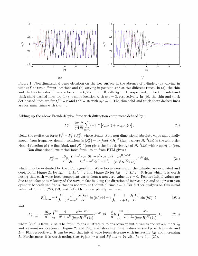
The wave-maker does a harmonic motion at the equilibrium position. Figure 1a describes the wavesat two fixed locations varying in time t/T . The thin and thick dot-dashed lines are obtained at x/λ = −1and x = 0 with k0c = 1 and L/λ = 2, respectively. λ represents the wave length λ = 2π/k0. The thinsolid and thick short dashed lines are time history at same location x/λ = −3 and x = 0 with k0c = 3 andL/λ = 6, respectively. Corresponding ratios of wave length and diameter are λ/(2c) = {π, π/3}. Timeevolution of the wave generation from initially rest to steady-state can be observed. Spatial profiles oftransient waves with wavefronts are shown in Figure 1b from the same position x = −L. The thin andthick dot-dashed lines for t/T = 8 and t/T = 16 with k0c = 1 start from x/λ = −2, while the thin solidand thick short dashed lines for t/T = 8 and t/T = 16 with k0c = 3 start from x/λ = −6.

Take a further analysis of wave elevation on the free surface ηI given in (3a). According to theasymptotic analysis, when time t is sufficiently large for any fixed position, or when time t is fixed, forany position far from the wave-maker, we correspondingly have :

limt→∞

η(x, t) = A sin[ωt− k0(x+ L)], and limx→∞

η(x, t) = 0, (21)

where the first equation represents steady-state plane progressive waves after some periods as shown inFigure 1a for x = 0 and x = −L/2, and the second equation approximately describes the existence ofwavefronts. It can be observed that there exists a maximum of wave elevation before the waves reachsteady-state.

3.2 Wave forces

When the potential Φ in (18) takes the form of ΦI in (2a), the non-dimensional Froude-Krylov forceF Ix due to incoming waves is :

F Ix = 2πJ1(k0c)

k0ccos(k0L) cos(ωt)− 4k0−

∫ ∞0

J1(kc)

kcsin(kL)

cos(βt)

k2 − k20dk. (22)

6

-1.5

-1

-0.5

0

0.5

1

1.5

0 4 8 12 16 20 24

ηI/A

t/T

-1.5

-1

-0.5

0

0.5

1

1.5

0 4 8 12 16 20 24

ηI/A

t/T

(a)

-1.5

-1

-0.5

0

0.5

1

1.5

-6 -2 2 6 10 14 18

ηI/A

x/λ

-1.5

-1

-0.5

0

0.5

1

1.5

-6 -2 2 6 10 14 18

ηI/A

x/λ

(b)

Figure 1: Non-dimensional wave elevation on the free surface in the absence of cylinder, (a) varying intime t/T at two different locations and (b) varying in position x/λ at two different times. In (a), the thinand thick dot-dashed lines are for x = −L/2 and x = 0 with k0c = 1, respectively. The thin solid andthick short dashed lines are for the same location with k0c = 3, respectively. In (b), the thin and thickdot-dashed lines are for t/T = 8 and t/T = 16 with k0c = 1. The thin solid and thick short dashed linesare for same times with k0c = 3.

Adding up the above Froude-Krylov force with diffraction component defined by :

FDx =2π

gA

∂

∂t

∞∑m=0

(−1)m[φm1(t) + φm(−1)(t)

], (23)

yields the excitation force FEx = F Ix +FDx , whose steady-state non-dimensional absolute value analytically

known from frequency domain solutions is |FEx | = 4/(k0c)2/|H(1)′

1 (k0c)|, where H(1)n (kc) is the nth order

Hankel function of the first kind, and H(1)′

n (kc) gives the first derivative of H(1)n (kc) with respect to (kc).

Non-dimensional excitation force formulation from ETM gives :

FEx = −16

π<∫ ∞0

ω2 cos (βt)− β2 cos (ωt)

(β2 − ω2)(β2 + ω2)

βeikL+iβt′

(kc)2H(1)′

1 (kc)e−iβt

′dβ, (24)

which may be evaluated by the FFT algorithm. Wave forces exerting on the cylinder are evaluated anddepicted in Figure 2a for k0c = 1, L/λ = 2 and Figure 2b for k0c = 3, L/λ = 6, from which it is worthnoting that each wave force component varies from a non-zero value at t = 0. Positive initial values aredue to the fact that velocity of the wave-maker is along the direction of increasing x and the pressure oncylinder beneath the free surface is not zero at the initial time t = 0. For further analysis on this initialvalue, let t = 0 in (22), (23) and (24). Or more explicitly, we have :

F Ix∣∣t=0

= 8

∫ ∞0

β

β2 + ω2

J1(kc)

kcsin (kL)dβ = 4

∫ ∞0

1

k + k0

J1(kc)

kcsin (kL)dk, (25a)

and

FEx∣∣t=0

=16

π<∫ ∞0

β

β2 + ω2

eikL+iβt′

(kc)2H(1)′

1 (kc)e−iβt

′dβ =

8

π<∫ ∞0

1

k + k0

eikL

(kc)2H(1)′

1 (kc)dk, (25b)

where (25b) is from ETM. The formulations illustrate relations between initial values and wavenumber k0and wave-maker location L. Figure 2c and Figure 2d show the initial values versus k0c with L = 4π andL = 10π, respectively. It can be seen that initial wave forces decrease with increasing k0c and increasingL. Furthermore, it is worth noting that F Ix |t=0 → π and FEx |t=0 → 2π with k0 → 0 in (25).

7

-6

-4

-2

0

2

4

6

0 2 4 6 8 10

Fx

t/T

-6

-4

-2

0

2

4

6

0 2 4 6 8 10

Fx

t/T

(a)

-0.6

-0.4

-0.2

0

0.2

0.4

0.6

0 2 4 6 8 10

Fx

t/T

-0.6

-0.4

-0.2

0

0.2

0.4

0.6

0 2 4 6 8 10

Fx

t/T

(b)

0

0.5

1

1.5

2

2.5

0 0.5 1 1.5 2 2.5 3 3.5 4 4.5 5

Fx

k0c

0

0.5

1

1.5

2

2.5

0 0.2 0.4 0.6 0.8 1

(c)

0

0.5

1

1.5

2

2.5

0 0.5 1 1.5 2 2.5 3 3.5 4 4.5 5

Fx

k0c

0

0.5

1

1.5

2

2.5

0 0.2 0.4 0.6 0.8 1

(d)

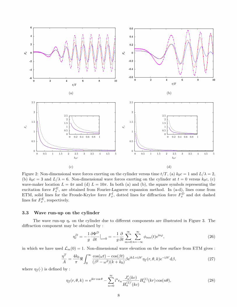
Figure 2: Non-dimensional wave forces exerting on the cylinder versus time t/T , (a) k0c = 1 and L/λ = 2,(b) k0c = 3 and L/λ = 6. Non-dimensional wave forces exerting on the cylinder at t = 0 versus k0c, (c)wave-maker location L = 4π and (d) L = 10π. In both (a) and (b), the square symbols representing theexcitation force FEx , are obtained from Fourier-Laguerre expansion method. In (a-d), lines come fromETM, solid lines for the Froude-Krylov force F Ix , dotted lines for diffraction force FDx and dot dashedlines for FEx , respectively.

3.3 Wave run-up on the cylinder

The wave run-up ηr on the cylinder due to different components are illustrated in Figure 3. Thediffraction component may be obtained by :

ηDr = −1

g

∂ΦD

∂t

∣∣z=0

= −1

g

∂

∂t

∞∑m=0

∞∑n=−∞

φmn(t)einϕ, (26)

in which we have used Lm(0) = 1. Non-dimensional wave elevation on the free surface from ETM gives :

ηT

A=

4k0π<∫ ∞0

cos(ωt)− cos(βt)

(β2 − ω2)(k + k0)βeikL+iβt′ηf (r, θ, k)e−iβt

′dβ, (27)

where ηf (·) is defined by :

ηf (r, θ, k) = eikr cos θ −∞∑n=0

inεnJ ′n(kc)

H(1)′n (kc)

H(1)n (kr) cos(nθ), (28)

8

-2

-1

0

1

2

0 2 4 6 8 10

η r/A

t/T

-2

-1

0

1

2

0 2 4 6 8 10

η r/A

t/T

(a)

-1.2

-0.6

0

0.6

1.2

0 2 4 6 8 10

η r/A

t/T

-1.2

-0.6

0

0.6

1.2

0 2 4 6 8 10

η r/A

t/T

(b)

-0.6

-0.4

-0.2

0

0.2

0.4

0.6

0 2 4 6 8 10

η r/A

t/T

-0.6

-0.4

-0.2

0

0.2

0.4

0.6

0 2 4 6 8 10

η r/A

t/T

(c)

-0.2

-0.1

0

0.1

0.2

0 2 4 6 8 10

η r/A

t/T

-0.2

-0.1

0

0.1

0.2

0 2 4 6 8 10

η r/A

t/T

(d)

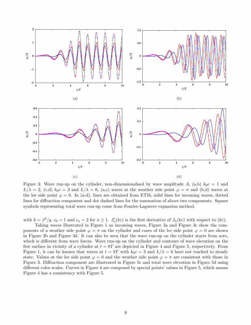
Figure 3: Wave run-up on the cylinder, non-dimensionalised by wave amplitude A, (a,b) k0c = 1 andL/λ = 2, (c,d) k0c = 3 and L/λ = 6, (a,c) waves at the weather side point ϕ = π and (b,d) waves atthe lee side point ϕ = 0. In (a-d), lines are obtained from ETM, solid lines for incoming waves, dottedlines for diffraction component and dot dashed lines for the summation of above two components. Squaresymbols representing total wave run-up come from Fourier-Laguerre expansion method.

with k = β2/g, ε0 = 1 and εn = 2 for n ≥ 1. J ′n(kc) is the first derivative of Jn(kc) with respect to (kc).Taking waves illustrated in Figure 1 as incoming waves, Figure 3a and Figure 3c show the com-

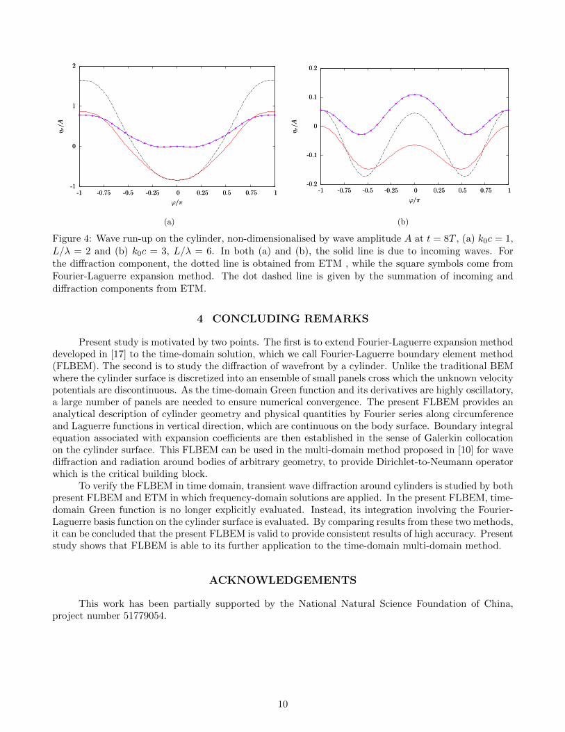
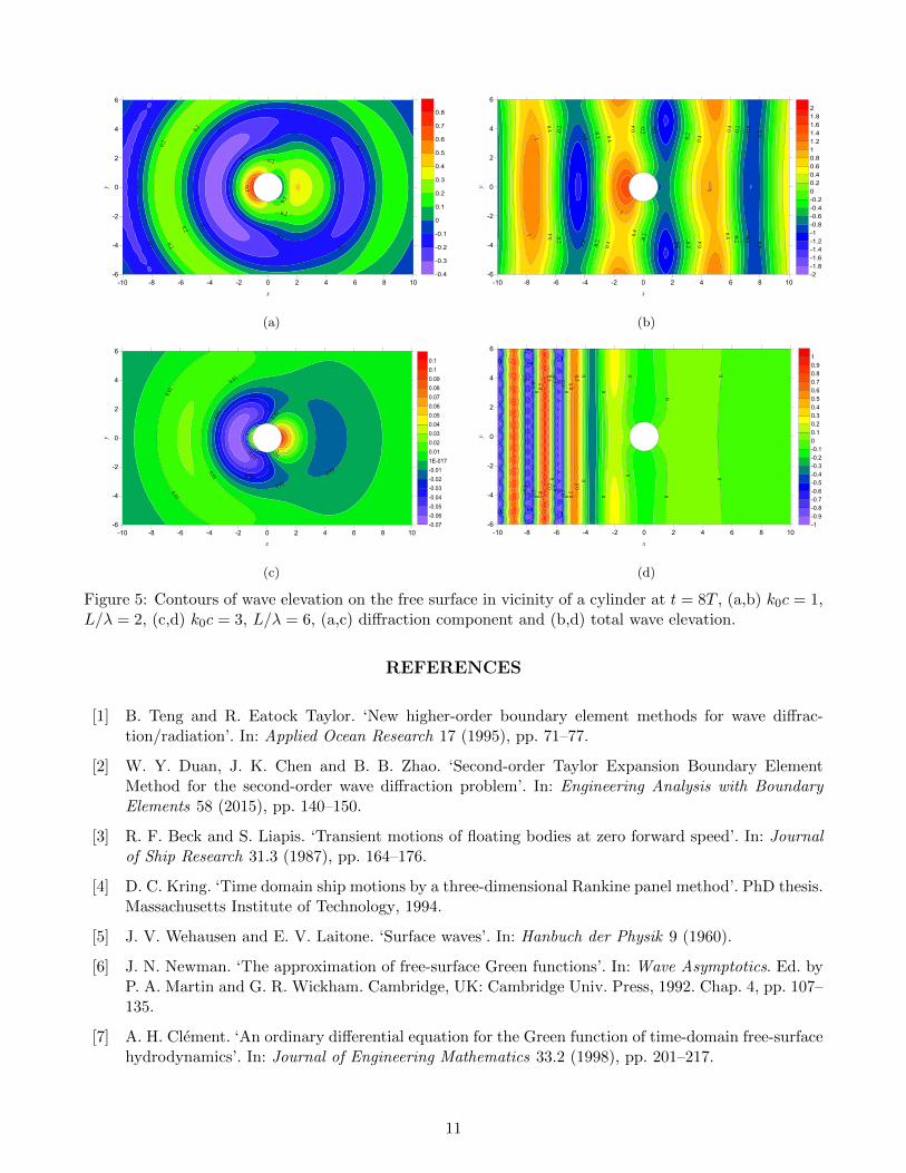
ponents of a weather side point ϕ = π on the cylinder and cases of the lee side point ϕ = 0 are shownin Figure 3b and Figure 3d. It can also be seen that the wave run-up on the cylinder starts from zero,which is different from wave forces. Wave run-up on the cylinder and contours of wave elevation on thefree surface in vicinity of a cylinder at t = 8T are depicted in Figure 4 and Figure 5, respectively. FromFigure 1, it can be known that waves at t = 8T with k0c = 3 and L/λ = 6 have not reached to steadystate. Values at the lee side point ϕ = 0 and the weather side point ϕ = π are consistent with those inFigure 3. Diffraction component are illustrated in Figure 5c and total wave elevation in Figure 5d usingdifferent color scales. Curves in Figure 4 are composed by special points’ values in Figure 5, which meansFigure 4 has a consistency with Figure 5.

9

-1

0

1

2

-1 -0.75 -0.5 -0.25 0 0.25 0.5 0.75 1

η r/A

φ/π

-1

0

1

2

-1 -0.75 -0.5 -0.25 0 0.25 0.5 0.75 1

η r/A

φ/π

(a)

-0.2

-0.1

0

0.1

0.2

-1 -0.75 -0.5 -0.25 0 0.25 0.5 0.75 1

η r/A

φ/π

-0.2

-0.1

0

0.1

0.2

-1 -0.75 -0.5 -0.25 0 0.25 0.5 0.75 1

η r/A

φ/π

(b)

Figure 4: Wave run-up on the cylinder, non-dimensionalised by wave amplitude A at t = 8T , (a) k0c = 1,L/λ = 2 and (b) k0c = 3, L/λ = 6. In both (a) and (b), the solid line is due to incoming waves. Forthe diffraction component, the dotted line is obtained from ETM , while the square symbols come fromFourier-Laguerre expansion method. The dot dashed line is given by the summation of incoming anddiffraction components from ETM.

4 CONCLUDING REMARKS

Present study is motivated by two points. The first is to extend Fourier-Laguerre expansion methoddeveloped in [17] to the time-domain solution, which we call Fourier-Laguerre boundary element method(FLBEM). The second is to study the diffraction of wavefront by a cylinder. Unlike the traditional BEMwhere the cylinder surface is discretized into an ensemble of small panels cross which the unknown velocitypotentials are discontinuous. As the time-domain Green function and its derivatives are highly oscillatory,a large number of panels are needed to ensure numerical convergence. The present FLBEM provides ananalytical description of cylinder geometry and physical quantities by Fourier series along circumferenceand Laguerre functions in vertical direction, which are continuous on the body surface. Boundary integralequation associated with expansion coefficients are then established in the sense of Galerkin collocationon the cylinder surface. This FLBEM can be used in the multi-domain method proposed in [10] for wavediffraction and radiation around bodies of arbitrary geometry, to provide Dirichlet-to-Neumann operatorwhich is the critical building block.

To verify the FLBEM in time domain, transient wave diffraction around cylinders is studied by bothpresent FLBEM and ETM in which frequency-domain solutions are applied. In the present FLBEM, time-domain Green function is no longer explicitly evaluated. Instead, its integration involving the Fourier-Laguerre basis function on the cylinder surface is evaluated. By comparing results from these two methods,it can be concluded that the present FLBEM is valid to provide consistent results of high accuracy. Presentstudy shows that FLBEM is able to its further application to the time-domain multi-domain method.

ACKNOWLEDGEMENTS

This work has been partially supported by the National Natural Science Foundation of China,project number 51779054.

10

-0.1

-0.1

-0.1

-0.1

-0.1

-0.1

-0.1

-0.1 -0.1

0.2

0.2

0.2

0.2

0.2

0.2

0.2

0.5

-10 -8 -6 -4 -2 0 2 4 6 8 10x

-6

-4

-2

0

2

4

6y

-0.4

-0.3

-0.2

-0.1

0

0.1

0.2

0.3

0.4

0.5

0.6

0.7

0.8

(a)

-0.8 -0.8

-0.8 -0.8

-0.8

-0.8-0.8

-0.8

-0.2

-0.2

-0.2

-0.2

-0.2

-0.2-0.2

-0.2

-0.2

-0.2

0.4

0.4

0.4

0.4

0.4

0.4

0.4

0.4

0.4

0.4

11

1

1

-10 -8 -6 -4 -2 0 2 4 6 8 10x

-6

-4

-2

0

2

4

6

y

-2-1.8-1.6-1.4-1.2-1-0.8-0.6-0.4-0.200.20.40.60.811.21.41.61.82

(b)

-0.05

-0.03

-0.03

-0.01

-0.01

-0.01

-0.01

0.01

0.01

0.01

0.01

0.010.03

-10 -8 -6 -4 -2 0 2 4 6 8 10x

-6

-4

-2

0

2

4

6

y

-0.07-0.06-0.05-0.04-0.03-0.02-0.011E-0170.010.020.030.040.050.060.070.080.090.10.1

(c)

-0.5

-0.5

-0.5

-0.5

-0.5

-0.5

-0.5

-0.5

00

0

0

0

0

0

0

00

0

0

00

00

0.5

0.5

0.5

0.5

0.5

0.5

0.5

0.5

-10 -8 -6 -4 -2 0 2 4 6 8 10x

-6

-4

-2

0

2

4

6

y

-1-0.9-0.8-0.7-0.6-0.5-0.4-0.3-0.2-0.100.10.20.30.40.50.60.70.80.91

(d)

Figure 5: Contours of wave elevation on the free surface in vicinity of a cylinder at t = 8T , (a,b) k0c = 1,L/λ = 2, (c,d) k0c = 3, L/λ = 6, (a,c) diffraction component and (b,d) total wave elevation.

REFERENCES

[1] B. Teng and R. Eatock Taylor. ‘New higher-order boundary element methods for wave diffrac-tion/radiation’. In: Applied Ocean Research 17 (1995), pp. 71–77.

[2] W. Y. Duan, J. K. Chen and B. B. Zhao. ‘Second-order Taylor Expansion Boundary ElementMethod for the second-order wave diffraction problem’. In: Engineering Analysis with BoundaryElements 58 (2015), pp. 140–150.

[3] R. F. Beck and S. Liapis. ‘Transient motions of floating bodies at zero forward speed’. In: Journalof Ship Research 31.3 (1987), pp. 164–176.

[4] D. C. Kring. ‘Time domain ship motions by a three-dimensional Rankine panel method’. PhD thesis.Massachusetts Institute of Technology, 1994.

[5] J. V. Wehausen and E. V. Laitone. ‘Surface waves’. In: Hanbuch der Physik 9 (1960).

[6] J. N. Newman. ‘The approximation of free-surface Green functions’. In: Wave Asymptotics. Ed. byP. A. Martin and G. R. Wickham. Cambridge, UK: Cambridge Univ. Press, 1992. Chap. 4, pp. 107–135.

[7] A. H. Clement. ‘An ordinary differential equation for the Green function of time-domain free-surfacehydrodynamics’. In: Journal of Engineering Mathematics 33.2 (1998), pp. 201–217.

11

[8] S. K. Liu and A. D. Papanikolaou. ‘Time-domain hybrid method for simulating large amplitudemotions of ships advancing in waves’. In: International Journal of Naval Architecture and OceanEngineering 3.1 (2011), pp. 72–79.

[9] K. Tang, R. C. Zhu, G. P. Miao and J. Fan. ‘Domain Decomposition and Matching for Time-DomainAnalysis of Motions of Ships Advancing in Head Sea’. In: China Ocean Engineering 28.4 (2014),pp. 433–444.

[10] X. B. Chen and H. Liang. ‘Wavy properties and analytical modeling of free-surface flows in thedevelopment of the multi-domain method’. In: Journal of Hydrodynamics 28.6 (2016), pp. 971–976.

[11] T. H. Havelock. ‘The pressure of water waves upon a fixed obstacle’. In: Proceedings of the RoyalSociety of London A: Mathematical, Physical and Engineering Sciences 175.963 (1940), pp. 409–421.

[12] R. C. Mac Camy and R. A. Fuchs. Wave forces on piles: A diffraction theory. U.S. Army CoastalEngineering Research Center (Formerly Beach Erosion Board), Technical Memorandum No. 69,1954.

[13] R. Eatock Taylor. ‘On Modelling the Diffraction of Water Waves’. In: Ship Technology Research54.2 (2007), pp. 54–80.

[14] M. Isaacson and K. F. Cheung. ‘Time-domain Second-order Wave Diffraction in Three Dimensions’.In: Journal of Waterway Port Coastal and Ocean Engineering 118.5 (1992), pp. 496–516.

[15] W. Bai and B. Teng. ‘Second-Order Wave Diffraction Around 3-D Bodies by A Time-DomainMethod’. In: China Ocean Engineering 15.1 (2001), pp. 73–84.

[16] C. Z. Wang and G. X. Wu. ‘Time domain analysis of second-order wave diffraction by an array ofvertical cylinders’. In: Journal of Fluids and Structures 23.4 (2007), pp. 605–631.

[17] H. Liang and X. B. Chen. ‘A new multi-domain method based on an analytical control surface forlinear and second-order mean drift wave loads on floating bodies’. In: Journal of ComputationalPhysics 347 (2017), pp. 506–532.

[18] X. B. Chen, H. Liang, R. P. Li and X. Y. Feng. ‘Ship seakeeping hydrodynamics by multi-domainmethod’. In: Proc. 32nd Symposium on Naval Hydrodynamics, Hamburg, Germany. 2018.

[19] S. W. Joo, W. W. Schultz and A. F. Messiter. ‘An analysis of the initial-value wavemaker problem’.In: Journal of Fluid Mechanics 214.214 (1990), pp. 161–183.

[20] Y. S. Dai and W. Z. He. ‘The Transient Solution of Plane Progressive Waves’. In: China OceanEngineering 7.3 (1993), pp. 305–312.

[21] X. B. Chen and R. P. Li. ‘Reformulation of wavenumber integrals describing transient waves’. In:Journal of Engineering Mathematics 115 (2019), pp. 121–140.

[22] X. B. Chen, B. B. Zhao and R. P. Li. ‘Mysterious wavefront uncovered’. In: Proc. 34th Intl Workshopon Water Waves and Floating Bodies, Newcastle, Australia. 2019.

[23] M. Abramowitz and I. A. Stegun. Handbook of Mathematical Functions: with Formulas, Graphs,and Mathematical Tables. 55. National Bureau of Standards, 1964.

12