Universidade de Lisboa

Faculdade de Ciências

Departamento de Engenharia Geográfica Geofísica e Energia

Development of photovoltaic systems with

concentration

Filipa Reis

Doutoramento em Sistemas Sustentáveis de Energia

2013

Universidade de Lisboa

Faculdade de Ciências

Departamento de Engenharia Geográfica Geofísica e Energia

Development of photovoltaic systems with

concentration

Filipa Reis

Tese orientada pelo Professor Doutor Miguel Centeno Brito e pelo Doutor

Gianfranco Sorasio, especialmente elaborada para a obtenção do grau de

Doutor em Sistemas Sustentáveis de Energia.

2013

I

Agradecimentos

Em primeiro lugar, exprimo a maior gratidão ao Professor Miguel Centeno Brito por me ter

recebido no nosso grupo de investigação e também, pelo seu inexcedível apoio profissional e pessoal, sem

o qual não seria possível realizar esta tese. E, ainda, manifesto-lhe elevado reconhecimento pela paciência

e pelas inúmeras horas dedicadas a ler esta tese, bem como por todos os trabalhos daí oriundos, com

relevo para os seus sapientes comentários, sempre construtivos. Obrigada, Miguel!

A todos os Professores do nosso grupo de investigação, nomeadamente o Professor Jorge Maia

Alves, o Professor João Serra, o Professor Killian Lobato e o Professor António Vallêra, que se

disponibilizaram para partilhar comigo os seus vastos conhecimentos, na área do fotovoltaico, e que, em

muitos casos, deram um contributo fundamental para alguns desafios deste trabalho, estou

penhoradamente grata.

Gostaria também de agradecer a toda a equipa da WS Energia e, em particular ao Doutor

Gianfranco Sorasio, que despertou o meu interesse por esta área e me incentivou no sentido de iniciar este

trabalho, e ainda ao Doutor João Wemans e ao Doutor Luís Pina, e, bem assim, ao João Mendes Lopes e

ao Sebastião Coelho, com quem trabalhei diretamente no desenvolvimento do projecto HSun. Também

agradeço à Doutora Victoria Corregidor, com a qual igualmente trabalhei no início do lançamento do

projecto HSun e que sempre se mostrou disponível para colaborar comigo.

Um especial agradecimento a todos os meus Colegas que me acompanharam no dia-a-dia deste

trabalho, em particular: ao Ivo Costa, por todas as “ideias engenhocas” que me permitiram colocar em

prática grande parte do trabalho experimental; ao David Pera, por me ter proporcionado uma formação

intensiva em SolidWorks; e ao André Augusto e Pierre Bellanger pela constante boa disposição.

Agradeço ainda ao Doutor Mauro Pravettoni, que me possibilitou todo o trabalho experimental

necessário à caracterização de células em condições de radiação elevada e não homogénea, cujos

resultados foram fundamentais para a validação do modelo desenvolvido. À LOGICA E.M. e, em

particular ao Nuno Pereira, deixo registados também os meus agradecimentos, por terem disponibilizado

o simulador solar para a caracterização de células em condições Standard. Agradeço à Lobosolar, por me

ter facultado o laboratório, bem como apoiado no estudo de envelhecimento do sistema DoubleSun.

Para o trabalho apresentado nesta tese foi também relevante a colaboração de todos os alunos

com quem trabalhei. Assim, agradeço à Carina Ramos, por ter colaborado comigo, aquando da sua tese de

mestrado, a qual se focou no desenvolvimento do receptor do sistema HSun; aos alunos Diogo Botelho,

Joana Silva e Ricardo Leandro, que desenvolveram comigo, no âmbito do seu projeto final de

licenciatura, o estudo do desempenho de sistemas fotovoltaicos instalados em Portugal continental; e aos

alunos Catarina Guerreiro, Fábio Batista e Tomás Pimentel, que desenvolveram também comigo o projeto

final de licenciatura, dando um contributo essencial ao estudo experimental do efeito de perfis de

temperatura não-uniformes no desempenho de uma célula. Para este último projeto foi também muito

importante o contributo dado pelo Ricardo Pereira, no apoio a todo o trabalho que decorreu na oficina.

Gostaria ainda de agradecer a todos os meus Amigos e Família, em especial ao Francisco Alves

e aos meus Pais, por todo o apoio que generosamente me prestaram, o qual considero que foi sem dúvida

fundamental para a realização deste trabalho.

Por fim, agradeço o apoio da FCT através da bolsa SFRH/BD/45328/2008.

A todos, Muito Obrigada!

II

III

Abstract

The concept of Concentration Photovoltaic (CPV) systems appeared as an attempt to reduce the

cost of Photovoltaic (PV) technology. In these systems, savings are achieved by the reduction of the area

of the expensive PV cell which is compensated by the increase in the light intensity on the device through

less expensive optical elements. This thesis focus on two main CPV systems: i) the DoubleSun®

technology, a low CPV system, already commercialized; and ii) a new medium CPV system, the HSun

technology.

Regarding the DoubleSun®, the on-field performance and ageing tests are addressed,

highlighting the main challenges that a CPV system has to face under outdoor exposure. Such results

were relevant for the development of a new CPV system concept, the HSun, whose main target is to

achieve grid parity. A Levelized Cost of Electricity (LCoE) analysis was performed showing that this

objective can only be achieved with a concentration factor between 15-20 suns and integrating high

efficiency silicon solar cells.

Within the HSun project, this thesis focuses on the CPV receiver whose design, development,

assembly, validation and optimization are discussed in detail. The analysis of its thermal behaviour is

addressed through CFD-FEA in a model implemented in SolidWorks which determines the temperature

profile across the solar cells showing that its integration on the HSun could be optimized to decrease the

average temperature of the cell by about 60°C. Since both illumination and temperature profiles are

spatially inhomogeneous, a distributed solar cell electric model is developed in order to understand and

fully describe the behaviour of solar cells under such operating conditions. The model was experimentally

validated and then applied to the optimization of the front grid of the solar cells on the HSun showing the

efficiency may be increased by 1.5% if front grid design integrates more 21 fingers.

Keywords: Photovoltaic, Concentration photovoltaic systems, Silicon solar cell model, Inhomogeneous

irradiation, Inhomogeneous temperature

IV

V

Resumo

O conceito de sistemas de Concentração Fotovoltaica (CPV) surgiu na tentativa de reduzir o

custo da tecnologia Fotovoltaica (PV). Nestes sistemas, a área das células solares, elemento caro, é

reduzida e compensada pelo aumento da intensidade da radiação no dispositivo através de elementos

ópticos, menos caros. Esta tese foca-se em dois sistemas CPV: i) a tecnologia DoubleSun®, um sistema

de baixa concentração, em comercialização; e ii) um novo sistema de média concentração, a tecnologia

HSun.

Relativamente ao sistema DoubleSun®, este foi estudado em termos de desempenho em terreno

e de testes de envelhecimento, destacando-se os maiores desafios que um sistema CPV enfrenta quando

instalado no exterior. Tais resultados foram relevantes para o desenvolvimento de um novo conceito de

sistema CPV, o HSun, cujo objectivo principal é atingir a paridade de rede. Uma análise de Custo

Nivelado da Electricidade mostrou que tal meta é apenas alcançável com um factor de concentração entre

15-20 sóis e integrando células de silício de elevada eficiência.

No âmbito do projecto HSun, esta tese foca-se no receptor CPV cujo desenho, desenvolvimento,

integração, validação e optimização são discutidos em detalhe. A análise do seu comportamento térmico

foi abordada através de CFD-FEA num modelo implementado em Solidworks. Este modelo determina o

perfil de temperatura nas células e mostrou que a sua integração no HSun pode ser optimizada reduzindo

a temperatura média das células em 60°C. Uma vez que tanto o perfil de iluminação como o de

temperatura são espacialmente não uniformes, desenvolveu-se um modelo eléctrico distribuído da célula

solar para perceber e descrever integralmente o comportamento desta quando em funcionamento em tais

condições. O modelo foi experimentalmente validado e posteriormente aplicado à optimização dos

contactos frontais das células solares que integram o HSun demonstrando que a eficiência das células

pode subir 1,5% se forem adicionados 21 contactos frontais.

Palavras-Chave: Fotovoltaico, Sistemas de concentração fotovoltaica, Modelo da célula solar de silício,

Radiação não uniforme, Temperatura não uniforme.

VI

VII

Contents

PART I

Chapter 1 – Concentration Photovoltaics

1.1. Introduction 3

1.2. Terms and concepts 7

1.3. CPV configurations 8

1.3.1. Concentration factor 9

1.3.2. Concentrator optics 10

1.3.2.1. Refractive optics 10

1.3.2.2. Reflective optics 11

1.3.3. Solar cells for CPV 13

1.3.3.1. Point-contact solar cells 14

1.3.3.2. Metal-Wrap-Through (MWT) and Emitter-Wrap-Through (EWT) solar cells 15

1.3.3.3. Sliver solar cells 16

1.3.4. Cooling systems for CPV 17

1.3.5. Tracking systems for CPV 18

1.3.6. Noticeable systems on the historical development of CPV 21

References 25

Chapter 2 – Thermal model of HSun

2.1. The HSun concept 31

2.2. Solar cells for HSun system 32

2.2.1. Physics of silicon solar cells 32

2.2.2. Challenges faced when under concentrated irradiation 34

2.2.3. Solar cells characterization 37

2.2.3.1. Cell electric parameters at Standard Test Conditions 39

2.2.3.2. Series resistance measurement 40

VIII

2.2.3.3. Ideality factor 42

2.2.3.4. Thermal coefficients 44

2.3. HSun receiver 46

2.3.1. Interconnection 46

2.3.2. Preliminary design of the sub-receiver 48

2.3.3. First prototype 49

2.3.4. Second prototype 50

2.3.5. Final prototype 52

2.4. On-field demonstration 53

2.4.1. Sub-receiver 53

2.5. Conclusions 54

References 54

Chapter 3 – Thermal model of HSun

3.1. Experimental characterization 57

3.1.1. Experimental setup 57

3.1.2. Temperature of the solar cell 59

3.1.3. Thermal resistance 60

3.1.4. Experimental results 61

3.2. Validation of the CFD-FEA model 62

3.3. CFD-FEA model for the HSun receiver 64

3.3.1. Model development 64

3.3.2. Simulation results 67

3.4. Conclusions 68

References 68

Chapter 4 – Modelling CPV silicon solar cells

4.1. Introduction 69

4.1.1. Review of state of the art 70

4.1.2. Critical analysis of state of the art 73

IX

4.2. Model 74

4.3. Cell design 74

4.3.1. Electric circuit 75

4.3.2. Current source 76

4.3.3. Diode 77

4.3.4. Series resistance components 78

4.3.5. Model dynamics 79

4.4. Conclusions 79

References 80

Chapter 5 – Model implementation and sensitivity analysis

5.1. Case study solar cell 83

5.1.1. Series resistance components 84

5.1.1.1. Measurement of the front busbar resistance 84

5.1.1.2. Measurement of the front finger resistance 84

5.1.1.3. Measurement of the contact and emitter sheet resistance 85

5.2. Simulation results for STC 88

5.3. Sensitivity analysis 89

5.3.1. Irradiance 89

5.3.2. Diode ideality factor 89

5.3.3. Series resistance components 90

5.3.4. Shunt resistance 91

5.4. Conclusions 91

References 91

Chapter 6 – Validation of solar cell electric model

6.1. Introduction 93

6.2. Validation at STC 94

6.3. Validation for homogenous profiles 94

6.3.1. High intensity illumination 94

X

6.3.2. High intensity illumination and temperature 96

6.4. Validation for inhomogeneous profiles 96

6.4.1. Irradiation 96

6.4.2. Temperature 98

6.5. Conclusions 100

References 101

Chapter 7 – Case studies

7.1. Comparison with standard model regarding irradiation 103

7.1.1. High irradiation 104

7.1.2. Inhomogeneous irradiation 104

7.1.2.1. Influence of peak location 105

7.1.2.2. Influence of non-uniformity 106

7.1.2.3. Influence of peak intensity 106

7.2. Comparison with standard model regarding temperature 107

7.2.1. Inhomogeneous temperature 108

7.2.1.1. Influence of peak location 108

7.2.1.2. Influence of non-uniformity 109

7.2.1.3. Influence of peak intensity 109

7.3. Model implementation for optimization of HSun technology 110

7.4. Optimization of the cell’s front grid contact 112

7.5. Conclusions 114

References 115

XI

PART II

Introductory Note 119

Chapter 1 – Ageing of DoubleSun system

1.1. Introduction 121

1.2. Methods 122

1.2.1. Outdoor exposure test 123

1.2.2. Ultraviolet conditioning test 123

1.2.3. Off-axis beam test 124

1.3. Results 124

1.3.1. Outdoor exposure test 124

1.3.2. Ultraviolet conditioning test 125

1.3.3. Off-axis beam test 125

1.4. Conclusions 126

References 126

Chapter 2 – DoubleSun performance across mainland Portugal

2.1. Introduction 127

2.2. Case study 127

2.3. Systems performance 129

2.3.1. Annual energy 129

2.3.2. Output power 130

2.3.3. Concentration coefficients 132

2.3.3.1. Resource availability 132

2.3.3.2. Energy increase due to tracking 133

2.3.3.3. Energy increase due to mirrors 133

2.3.3.4. Concentration coefficient 134

2.4. Challenges faced by on-field systems 134

2.5. Conclusions 135

XII

References 135

Chapter 3 – Photovoltaic potencial in Terceira Island, Azores

3.1. Introduction 137

3.2. Resource characterization 138

3.3. Results 139

3.4. Conclusions 141

References 141

Chapter 4 – Levelized cost of electricity

4.1. Introduction 143

4.2. LCoE model and assumptions 143

4.2.1. Capacity costs 143

4.2.2. Annual costs 144

4.2.3. Annual energy 145

4.2.4. LCoE 145

4.3. Results 146

4.3.1. Capacity costs 146

4.3.2. LCoE 147

4.3.3. Effect of modules cost on the systems LCoE 147

4.4. Optimal concentration level for the HSun technology 148

4.4.1. Modifications on the LCoE model 149

4.4.2. LCoE for the HSun technology 150

4.5. Conclusions 151

References 152

Conclusions 153

Annexes

Annex A – CPV systems 157

XIII

List of Figures

PART I

Chapter 1 - Introduction

Fig. 1.1 - The principle of CPV optics using lens (on the left) and mirrors (on the right). 3

Fig. 1.2 - Global PV module price learning curve for c-Si wafer based and CdTe modules, 1979-

2015. Source: (IRENA 2012). 5

Fig. 1.3 - Residential PV price parity (size of bubbles refers to market size). Notice that the LCoE

is based on 6% weighted average cost of capital, 0.7%/year module degradation, 1% capex as

Operation and Maintenance (O&M) annually. $3.01/W capex assumed for 2012, $2/W for 2015.

Source: (Chase 2012).

5

Fig. 1.4 - Terms used for CPV ((IEC) 2007). 8

Fig. 1.5 - Criteria used in CPV classification. 8

Fig. 1.6 - Distribution of the CPV systems developed by 100 companies (Annex A, Table A.1)

according to the systems’s concentration factor. 9

Fig. 1.7 - Distribution of the CPV systems developed by 100 companies (Annex A, Table A.1)

according to the systems’ optics design. 10

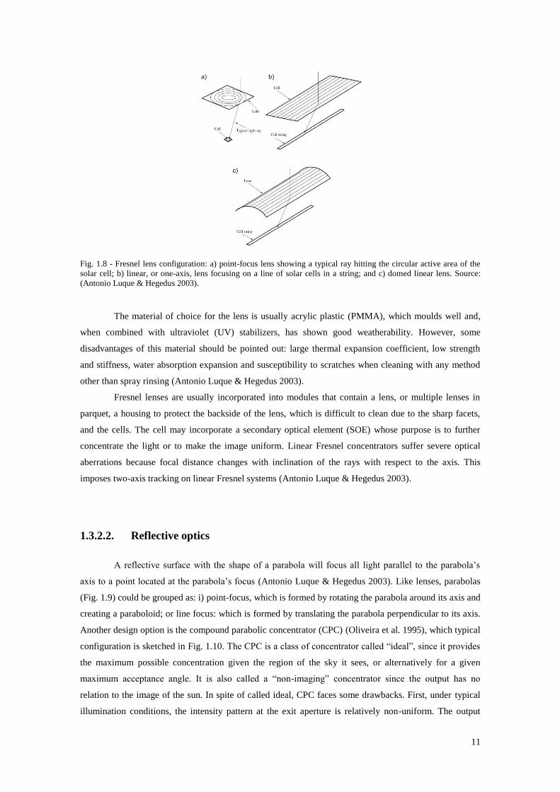
Fig. 1.8 - Fresnel lens configuration: a) point-focus lens showing a typical ray hitting the circular

active area of the solar cell; b) linear, or one-axis, lens focusing on a line of solar cells in a string;

and c) domed linear lens. Source: (Antonio Luque & Hegedus 2003).

11

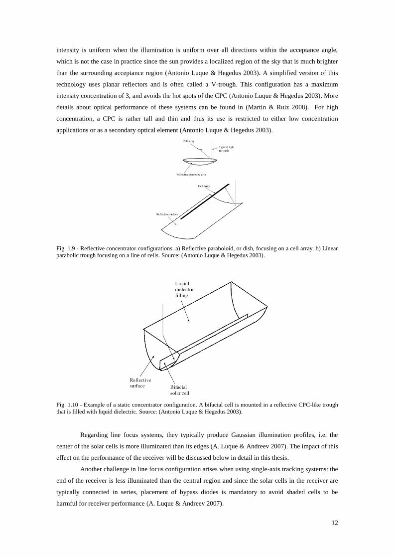
Fig. 1.9 - Reflective concentrator configurations. a) Reflective paraboloid, or dish, focusing on a

cell array. b) Linear parabolic trough focusing on a line of cells. Source: (Antonio Luque &

Hegedus 2003).

12

Fig. 1.10 - Example of a static concentrator configuration. A bifacial cell is mounted in a reflective

CPC-like trough that is filled with liquid dielectric. Source: (Antonio Luque & Hegedus 2003). 12

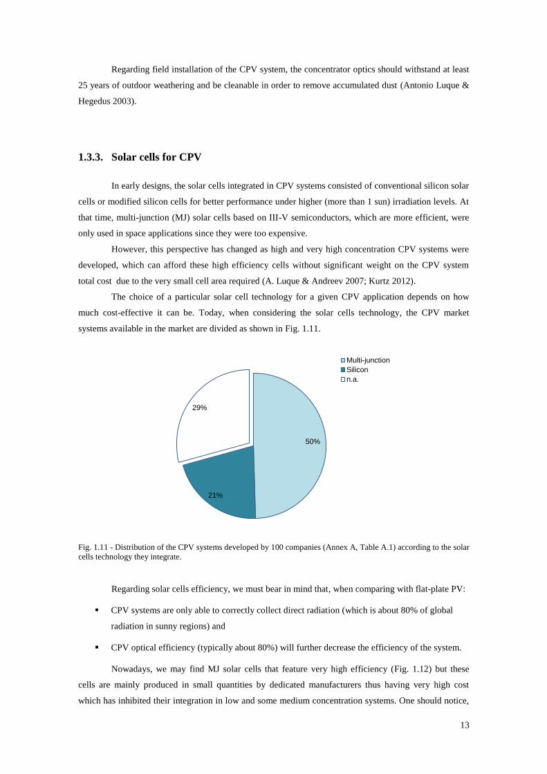
Fig. 1.11 - Distribution of the CPV systems developed by 100 companies (Annex A, Table A.1)

according to the solar cells technology they integrate. 13

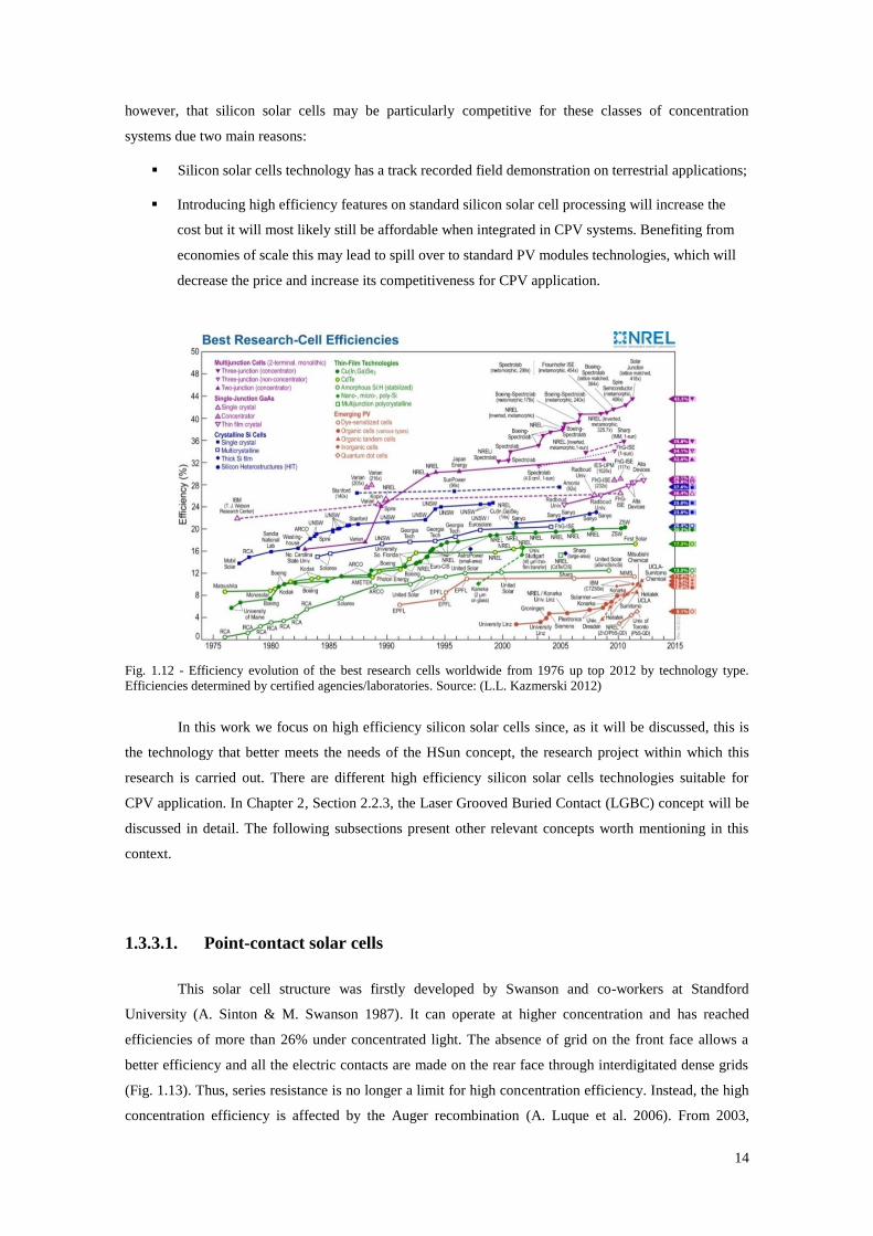
Fig. 1.12 - Efficiency evolution of the best research cells worldwide from 1976 up top 2012 by

technology type. Efficiencies determined by certified agencies/laboratories. Source: (L.L.

Kazmerski 2012)

14

Fig. 1.13 - SunPower A-300 solar cell. Source: (Lawrence L. Kazmerski 2006). 15

Fig. 1.14 - MWT solar cell: a) structure of the cell (Glunz 2007) and b) picture of a highly efficient

industrially feasible MWT silicon solar cell (Fellmeth et al. 2010). 15

Fig. 1.15 - Schematic drawing of an EWT solar cell of Advent Solar. Source: (Glunz 2007). 16

Fig. 1.16 - Schematic of sliver solar cells process and cell structure. Source: (Andrew Blakers et al.

2006). 17

Fig. 1.17 - Schematics of passive and active cooling systems. Source: (Anon n.d.). 18

XIV

Fig. 1.18 - Distribution of the CPV systems developed by 100 companies (Annex A, Table A.1)

regarding the type of tracking. 19

Fig. 1.19 - Two-axis tracking configurations: a) Two-axis tracker with elevation and azimuth

tracking mounted on a pedestal. b) Roll-tilt tracking arrangement using central torque tube. c) Roll-

tilt tracking arrangement using box frame. d) Turntable two-axis tracker. Source: (Antonio Luque

& Hegedus 2003).

20

Fig. 1.20 - One-axis tracking configurations: a) One-axis horizontal tracker with reflective trough;

b) One-axis polar axis tracker with reflective trough. Source: (Antonio Luque & Hegedus 2003). 21

Fig. 1.21 - EUCLIDES III concentrator a) installed at Stuttgard (Germany), including two arrays

for the 24X and 12X concentration levels and b) detail of the final receiver of the EUCLIDES III,

including the cells, the heat sink and the secondary mirrors. Source: (Marta Vivar et al. 2011).

22

Fig. 1.22 - HCPV system developed by Amonix: a) schematic of the system and b) photograph of

the system installed in Arizona Public Service’s Solar Test and Research (STAR) facility in 1994.

Source: (V Garboushian et al. 1996).

23

Fig. 1.23 - Concentration photovoltaic (CPV) system developed by Solar Systems Australian

company: a) Power station of 190kWp in Hermannsburg; b) detail of the MJ 33 kWp receiver.

Source: (Pierre J. Verlinden 2006).

23

Fig. 1.24 - Archimedes system: a) principle scheme of the structure and b) frontal view. Source:

(Klotz et al. 2001). 24

Fig. 1.25 - Combined Heat and Power System (CHAPS) at Australian National University: a)

picture of the system; and b) schematic of a cross-section of the receiver with the cells and cooling

system. Source: (M. Vivar et al. 2010).

24

Fig. 1.26 - Whitfield system: a) Whitfield system, b) components of a V-trough carrying the cell;

and c) close-up of the illumination spot on the cell also showing a bypass diode. Sources: (Bentley

et al. n.d.).

25

Chapter 2 – The HSun system

Fig. 2.1 - HSun module mounted on a two-axis tracking system. Courtesy of: WS Energia S.A. 31

Fig. 2.2 - Schematic of a PV solar cell. 33

Fig. 2.3 - Standard electric single-diode model for a solar cell. 33

Fig. 2.4 - Current-Voltage (I-V) curve and its main parameters for a solar cell. 34

Fig. 2.5 - Estimated power loss (Ploss) and efficiency (ε) as a function of the concentration level.

The dashed line represents the efficiency without considering the Joule losses. 36

Fig. 2.6 - Scanning Electron Microscope (SEM) image of a finger contact for a) NaREC and b)

Solartec solar cells. 38

Fig. 2.7 - NaREC solar cell and detail of the busbar. 38

Fig. 2.8 - Solartec solar cell: a) front surface and b) back surface. 39

Fig. 2.9 - Current density - Voltage (J-V) curves measured under STC for: a) NaREC and b)

Solartec solar cells at LOGICA E.M. 40

XV

Fig. 2.10 - Schematic of a) setup used in the OCVD method and b) expected V(t) curve. Source:

(D. K. Schroder 2006). 41

Fig. 2.11 - Curves obtained through the OCVD method for the NaREC solar cell when a current of

1.5 A is imposed. 42

Fig. 2.12 - Semi-logarithmic plot for the NaREC and Solartec cells, respectively. 43

Fig. 2.13 - Measured a) I-V curves for the NaREC solar cells at 1000 W/m2 and different

temperatures: 25, 30, 40, 50 and 60°C. Through the Voc and Isc registered in these curves, the

thermal coefficients for the b) Voc and c) Isc were calculated.

45

Fig. 2.14 - Measured a) I-V curves for the Solartec solar cells at 1000 W/m2 and different

temperatures: 25, 30, 40, 50 and 60°C. Through the Voc and Isc registered in these curves, the

thermal coefficients for the b) Voc and c) Isc were calculated.

46

Fig. 2.15 - Soldering process of a ribbon on the solar cell busbar: a) positioning of the solar cell

into the aluminium base; b) pen flux to apply some flux on the cell’s busbar in order to facilitate

solder adhesion between the cell and the ribbon; and c) positioning and soldering the tab to the

busbar through a soldering iron.

47

Fig. 2.16 - Maximum power (Pmp), Series resistance (Rs), Shunt resistance (Rsh) and Fill Factor

(FF) of the soldered cell as a percentage of the value obtained for the unsoldered cell. 48

Fig. 2.17 - Schematic of the first sub-receiver prototype. The cells are represented by the blue

rectangle and the interconnection between them are represented by the grey areas (when are

designed in the board) and the red tabs (when soldered to the cell).

48

Fig. 2.18 - Electrical scheme of the interconnection between solar cells in the first sub-receiver

prototype. 49

Fig. 2.19 - First receiver prototype with two series connected cells on the centre and two bypass

diodes on the borders. 50

Fig. 2.20 - Printed circuit board (PCB) and schematic of the components placement and

interconnection. 51

Fig. 2.21 - Finished sub-receiver including the PCB with the bypass diodes, and the soldered

ribbon interconnecting each cell to the neighbouring cell in a series connection. 51

Fig. 2.22 - Distribution of the sub-receivers within a certain range of Pmp: a) before and b) after the

re-soldering process. 52

Fig. 2.23 - Distribution of sub-receivers that are within a certain range of Pmp: a) before and b) after

the re-soldering process. 52

Fig. 2.24 - Sub-receiver mounted for on-field demonstration. Source: (Ramos 2011). 53

Fig. 2.25 - Short-circuit current (on the left) and open-circuit voltage (on the right) measured for

each solar cell (red bars) and for the sub-receiver (blue bar) under outdoor conditions: 800W/m2 of

irradiation and 30.5°C of ambient temperature, normalized to the Isc and Voc estimated expected for

the solar cell under such conditions (black dashed lines). Source: (Ramos 2011)

53

Chapter 3 – Thermal model of HSun

Fig. 3.1 - Schematic draw of the receiver in study. 57

XVI

Fig. 3.2 - Solar simulador: a) build at SESUL laboratory; b) schematic representation of the solar

simulator; and c) detail of the sample holder integrated in the solar simulator. 58

Fig. 3.3 - Schematic of the experimental apparatus for the measurement of the temperature of each

material. 59

Fig. 3.4- Equivalent thermal circuit of the receiver. 61

Fig. 3.5 - Cell temperature (squares) estimated by the Voc and temperature measured for material 2

(circles), material 3 (lozenges) and the sample holder (asterisk) during Run 1 (darker colours) and

Run 2 (lighter colours).

62

Fig. 3.6 - Temperatures obtained experimentally (Run 1 and Run 2) and by the model simulation. 63

Fig. 3.7 - Thermal resistances estimated using the temperatures obtained experimentally and by the

simulation. 63

Fig. 3.8 - Top view of the temperature distribution on the solar cell for a simulation of 19 suns: rear

surface of material 3 at 42ºC and an ambient temperature of 25ºC. 64

Fig. 3.9 - HSun structure considered for case study of the receiver thermal behaviour. 64

Fig. 3.10 - Schematic of the receiver layers (and the corresponding materials) from bottom to top. 66

Fig. 3.11 - Irradiation profile (suns) across the solar cell width (only considering the distance

between the busbar and the opposite edge of the cell). 66

Fig. 3.12 - Temperature profile on half of the receiver for: a) the case in which the receiver is 1.5

mm away from the primary optics behind it; and b) the case in which receiver’s back surface is

thermally connected to the back surface of the primary optics behind it. In the latter case it is also

shown a detail (b1) of the temperature profile across three solar cells.

67

Chapter 4 – Modelling CPV silicon solar cells

Fig. 4.1 - Lumped resistance model for a solar cell. 70

Fig. 4.2 - Decrease in a) open-circuit voltage (Voc) and b) efficiency (ε) against peak illumination

ratio. Each result is identified by the first author of the paper. 73

Fig. 4.3 - Design of: a) the solar cell considered as case study; b) a solar cell element; and c) the

equivalent electric circuit of a solar cell element. 75

Fig. 4.4 - Equivalent electric circuit for the elementary units located in: a) the semiconductor

region and b) the contact region. Depending on the cell region that is being considered, Rx may

become Rf (finger) or Rb (busbar).

76

Fig. 4.5 - Flowchart of the solar cell model implemented in Matlab/Simulink. 79

Chapter 5 – Model implementation and sensitivity analysis

Fig. 5.1 - Front grid pattern of a solar cell showing the placement of the probes for a four-point

measurement of the busbar resistance. 84

Fig. 5.2 - Position of the probes for a four-point measurement of the average finger resistance on a

solar cell with one busbar. Notice that in the case of one single busbar on the cell, the busbar is 85

XVII

removed from the cell to perform the measurement.

Fig. 5.3 - Front grid pattern of a slice of solar cell without busbars showing the placement of the

probes for a four-point measurement of the contact and emitter sheet resistances. 85

Fig. 5.4 - Plot for extracting the contact and emitter sheet resistances. 86

Fig. 5.5 - I-V curve measured and modelled under STC conditions. 88

Fig. 5.6 - Sensitivity of each parameter (Isc, Voc and Pmp) with respect to variations on the

irradiance. 89

Fig. 5.7 - Coefficients for: a) percentage variation of Voc and b) percentage variation of Pmp with

respect to the percentage variation of n plotted against the concentration/temperature levels for

different temperature/concentration, respectively.

90

Fig. 5.8 - Power loss versus series resistance components increase of 25%, 50% and 75.8% for: a)

1 sun and b) 15 suns. 90

Fig. 5.9 - Power loss versus variation in shunt resistance (Rsh) for a concentration level of 1 sun

(light blue diamond markers) and 15 suns (dark blue squared markers). 91

Chapter 6 – Validation of the solar cell electric model

Fig. 6.1 - Modelled (solid line) and experimental (squared markers) current-voltage (dark blue) and

power-voltage (light blue) curves for the solar cell in study under Standard Test Conditions (STC). 94

Fig. 6.2 - Modelled versus measured values for a) short-circuit current (dark blue squared markers)

and maximum power point (light blue triangle markers) and b) open-circuit voltage (blue circle

markers) for a solar cell homogeneously illuminated under different irradiance values within a

range between 1 and 30 suns and at 25°C.

95

Fig. 6.3 - Modelled versus measured value of Voc for a cell under 1 sun (light blue squared

markers), 11 suns (medium blue triangle markers) and 19 suns (dark blue circle markers) for

different solar cell temperatures. The Voc values are normalized to the Voc modelled and measured,

respectively, for the same irradiation conditions at 25°C.

96

Fig. 6.4 - Illumination profiles for a) stepwise illumination and b) Gaussian profiles. 98

Fig. 6.5 - Experimentally versus modelled results obtained for maximum power point for each

illumination profile. Notice that both experimental and modelled results are normalized with

respect to the results under STC.

97

Fig. 6.6 - Experimentally versus modelled results obtained for maximum power point for each

illumination profile. Notice that both experimental and modelled results are normalized with

respect to the homogeneous irradiation case at 15 suns and 25ºC.

98

Fig. 6.7 - Temperature profile (in °C) obtained for: a) the sample holder and b) the solar cell when

placed on it. 98

Fig. 6.8 – Sample holder. 99

Fig. 6.9 - Open-circuit voltage (Voc) measured (markers) and modelled (solid lines) for a solar cell

with i) homogeneous temperature distribution (black markers and line); ii) a temperature profile

whose maximum value is on the busbar (red markers and line); and iii) a temperature profile whose

minimum value is on the busbar (blue markers and line). Notice that the dashed lines correspond to

the trendline of the measured data.

99

XVIII

Chapter 7 – Case studies

Fig. 7.1 - Current estimated by the distributed model versus the current estimated by the standard

model for the same voltage at STC. The red dot represents the Impp point. 103

Fig. 7.2 - Maximum power point (Pmp), estimated by the conventional lumped model (dashed grey

line) and the distributed model (dashed black line) for different concentration levels. The

experimental values are also presented (blue squared markers).

104

Fig. 7.3 – Power loss of a solar cell inhomogeneously illuminated with respect to the power at

homogeneous irradiation distribution with an average of 29.2 suns. In the cell schematic the black

bar represents the cell busbar and the pallet of shades is illustrative of the highly illuminated

(white) and lower illuminated (dark grey) regions.

105

Fig. 7.4 - Maximum power point (Pmp) in as a percentage of the Pmp obtained for the homogeneous

illumination case with the same average illumination versus the parameter of irradiation

inhomogeneity, r.

106

Fig. 7.5 - Power loss of the inhomogeneous illuminated cells with respect to the homogeneously

illuminated with the same average irradiation plotted against the average irradiation on the cell. 107

Fig. 7.6 - Maximum power point (Pmp) estimated by the conventional lumped model (cross markers

with dashed black line) and the distributed model (squared markers with dashed light blue line) for

different temperatures.

107

Fig. 7.7 - Power loss of a solar cell when subjected to a non-uniform temperature profile with

respect to the power at homogeneous temperature distribution with the same average (49.6°C).

Notice that in the cell schematic, the black bar represents the cell busbar and the pallet of shades is

illustrative of the warmest (red) and colder (white) regions.

108

Fig. 7.8 - Open-circuit voltage obtained for a solar cell under different temperature profiles. The

results are shown against the t parameter and are normalised to the Voc obtained at STC. 109

Fig. 7.9 - Open circuit voltage (Voc) obtained for the solar cell under homogeneous (black solid line

with diamond markers) and inhomogeneous (red dashed lines with square markers) temperature

profiles.

109

Fig. 7.10 – Irradiation profile along the cell width: i) predicted by the Ray Tracing software (black

markers) and ii) interpolation to the data (red line). 110

Fig. 7.11 – Temperature profile for a solar cell located at the edge of the receiver. The black

markers correspond to the points obtained through CFD-FEA simulations in Solidworks while the

coloured surface corresponds to the interpolation performed to such points.

111

Fig. 7.12 – Curves obtained for a) Current-Voltage (I-V) and b) Power-Voltage (P-V) for a cell at

the middle (light blue line) and a cell at the edge of the receiver (dark blue line). The black dashed

line represents an I-V curve for a solar under homogeneous irradiation and temperature for the

average values found within the HSun cells.

112

Fig. 7.13 - Efficiency obtained for each solar cell design with respect to the efficiency obtained for

the original cell design plotted against the number of fingers. The solar cell under analysis presents

a radiation and temperature profiles similar to the solar cell located at the edge of the HSun

receiver. The red squared marker corresponds to the optimum number of fingers while the white

squared marker corresponds to the original solar cell.

113

Fig. 7.14 – Current-Voltage (I-V) curves obtained for each solar cell design (i.e. different number

of fingers) when considering the cell located at the edge of the HSun receiver. 113

XIX

PART II

Chapter 1 – Ageing of DoubleSun® system

Fig. 1.1 – DoubleSun® system installed at WS Energia laboratory in Oeiras, Portugal

(38º41’50’’N, 9º18’30’’W). Source: WS Energia S.A. 122

Fig. 1.2 - Prototype similar to DoubleSun® technology. 124

Fig. 1.3 - Current-Voltage (I-V) curve measured for the module under 1sun (dark blue squared

markers) and 1.85 suns (light blue triangle markers) a) before UV exposure and b) after UV

exposure. Notice the decrease of Isc in case b) when the module is integrated in the CPV system

(C=1.85).

125

Chapter 2 – DoubleSun® performance across mainland Portugal

Fig. 2.1 - Percentage distribution of the 110 PV systems across mainland Portugal. 128

Fig. 2.2 - Geographical distribution through mainland Portugal of the PV systems in analysis:

DoubleSun® (red dots) and flat plate (white dots). 128

Fig. 2.3 – Accumulated energy produced by the DoubleSun® (squared markers) and a flat-plate

(triangle markers) system from July 2009 to June 2010. In the up left corner the average annual

energy produced by each system during the period under analysis is presented with respect to the

flat-plate system annual energy.

129

Fig. 2.4 - Energy produced by month for: a) DoubleSun® and b) flat-plate systems installed across

mainland Portugal. 130

Fig. 2.5 - AC power of the DoubleSun® (blue) and Flat-plate systems (red) registered during a

clear day (solid lines) and daily average (dashed lines) for: a) December 2009 and b) June 2010.

The systems were installed in Lisbon.

131

Fig. 2.6 - Annual average of δ and δ* for different locations in Portugal mainland. 132

Fig. 2.7 - Annual average of γ for different locations in Portugal mainland. 133

Fig. 2.8 - Annual average of α and α* for different locations in Portugal mainland. 134

Fig. 2.9 - Annual average of R and R* for different locations in Portugal mainland. 134

Chapter 3 – Photovoltaic potential in Terceira Island, Azores

Fig. 3.1 - Group of Azores islands. Source: (Fans n.d.). 137

Fig. 3.2 - Daily profile of: a) global, b) direct, and c) diffuse irradiance (W/m2) measured during

2009 at Angra do Heroísmo, in Terceira Island. 138

Fig. 3.3 - Daily profile of the ambient temperature (°C) measured during 2009, in Angra do

Heroísmo. 139

Fig. 3.4 - Ratio of the AC power between: a) 2-axes tracking system and a flat plate system; b) the

DoubleSun® system and a tracking system; and c) the DoubleSun® system and a flat-plate system.

140

XX

Fig. 3.5 - Energy produced by a 2 axes tracking system and by a DoubleSun system normalized to

the energy produced by a flat-plate system. 140

Fig. 3.6 - Expected accumulated energy (kWh/kWp) produced by the flat-plate system, 2-axes

tracking system and the DoubleSun® system during 2009 in Angra do Heroismo. 141

Chapter 4 – Levelized cost of electricity

Fig. 4.1 - Energy (kWh/kWp) produced by each system configuration during its lifetime. 146

Fig. 4.2 - Cost of the main elements of each system as a percentage of the total cost of the system. 147

Fig. 4.3 - LCoE for the DoubleSun, two-axis tracker, one-axis tracker and the conventional flat-

plate system. 148

Fig. 4.4 - LCoE of the flat-plate system with respect to the LCoE of: i) a DoubleSun® system

(orange line); ii) a two-axis tracking system (dark blue line); and iii) a one-axis tracking system

(light blue line).

149

Fig. 4.5 - Levelized Cost of Electricity (LCoE) estimated for the HSun technology at different

concentration levels. 152

XXI

List of Tables

PART I

Chapter 2 - The HSun system

Table 2.1 - Solar cell dimensions. 39

Table 2.2 - Series resistance of the NaREC and Solartec solar cells estimated by different

methods. 42

Table 2.3 - Electrical parameters obtained through the I-V curve measured under STC of the

NaREC and Solartec solar cells. 43

Table 2.4 - Thermal coefficients for the short-circuit current (ki) and open-circuit voltage (kv)

estimated for the NaREC and Solartec solar cells. 46

Chapter 3 - Thermal model of HSun

Table 3.1 – Materials associated to the HSun receiver’s case study used in the CFD-FEA. 65

Chapter 4 - Modelling CPV silicon solar cells

Table 4.1 - Resistors developed for the model. 78

Chapter 5 - Model implementation and sensitivity analysis

Table 5.1 – Model input parameters. 83

Table 5.2 - Resistivities found in the literature. 87

Table 5.3 - Resistivities measured for the NaREC and Solartec cells. 88

Chapter 6 - Validation of the solar cell electric model

Table 6.1 - Experimentally measured solar cell parameters (dimensions, electric, thermal

coefficients and resistances) relevant for the implementation of the model. 94

Chapter 7 - Case studies

Table 7.1 – Minimum (Tmin), maximum (Tmax) and average (Tavg) temperature for the solar cell

located at the edge (Cell at edge) and at the middle (Cell at middle) of the receiver. 111

XXII

PART II

Chapter 1 - Ageing of DoubleSun® system

Table 1.1 - Typical electrical parameters of the modules used in the outdoor exposure test. 123

Table 1.2 - Electrical parameters of the module used in UV conditioning test. 124

Table 1.3 - Electrical parameters of the module before and after 6 months of outdoor exposure. 125

Chapter 4 - Levelized cost of electricity

Table 4.1 - Cost (€/Wp) of the components and installation of each PV system considered in the

present analysis (SOURCE: WS Energia). 145

Table 4.2 - Capacity costs that were modified for the HSun calculations. 151

XXIII

List of Variables

A Unit area in Simulink

Aactive Active area

AT Tracking area

C Concentration level

C0 Concentration of 1 sun, i.e. 1000 W/m2

CI Installation cost

CM Modules cost

CO Optics cost

CO&M Operation and maintenance cost

Copt Optimum concentration level

CT Tracker cost

d Space between fingers

dr Discount rate

dxe Length of the elementary emitter unit

dxf Length of the elementary finger unit

dy Emiter unit width

f Number of elements

FF Fillfactor

g Degradation rate

I Current

I0 Reverse saturation current

ic ratio between direct irradiation and normal irradiation

ID Diffusion diode current

Idiode Diode current

Iimposed Current imposed in the cell when performing OCVD method

Impp Current at maximum power point

Iph Photogenerated current

Isc Short-circuit current

Ish Current through the shunt resistor

j Number of fingers

Jsc Short-circuit current density

Jsc(STC) Short-circuit current density under STC

k Boltzmann constant (1.380 x 10-23

J/K)

ki Thermal coefficient for current

kV Thermal coefficient for voltage

L Cell length

XXIV

n Ideal factor of the diode

Pin Irradiance falling on the cell

PIR Peak Illumination Ratio

Ploss Power loss

Pmp Maximum power point

Psystem Power of the system

q Electron charge (1.602 x 10-19

C)

Q Radiation that falls on the cell

Qn Energy output per installed power

r Parameter that refers to the degree of illumination inhomogeneity on the cell

R Concentration coefficient

Ravg Average irradiance on the cell

Rbulk Bulk resistor

Rc Contact resistor

RCH Characteristic resistance

Re Emitter resistor

Rf Finger resistor

Rmax Maximum irradiance on the cell

Rmin Minimum irradiance on the cell

Rs Series resistance

rS Normalized series resistance

Rsh Shunt resistance

T Temperature

t Parameter that refers to the degree of temperature inhomogeneity on the cell

T0 Ambient temperature, 25°C

Tavg Average temperature on the cell

TLCC Total life cycle cost

Tmax Maximum temperature on the cell

Tmin Minimum temperature on the cell

TSTC Ambient temperature, 25°C

V Voltage

Vmpp Voltage at maximum power point

Voc Open-circuit voltage

Voc(STC) Open-circuit voltage at Standard Test Conditions (STC)

VT Thermal voltage

W Cell width

y Year of operation

Y Period under analysis

Z Busbar/Finger thickness

XXV

α parameter to evaluate the energy increase due to the mirrors

β Busbar width

γ Parameter to evaluate the energy increase due to tracking

δ Parameter to evaluate the resource availability

ΔR Difference between the maximum and minimum irradiance values

ΔT Difference between the maximum and minimum temperature values

ΔV Voltage drop due to series resistance

ε Efficiency

εa Efficiency of the active area

εo Optical efficiency

εsystem Efficiency of the system

ρc Contact resistivity

ρe Emitter resistivity

ω Finger width

XXVI

XXVII

List of Acronyms

ANU Australian National University

BOS Balance of system

CdTe Cadmium Telluride

CFD-FEA Computational Fluid Dynamics - Finite Element Analysis

CHAPS Combined Heat And Power System

CPV Concentration Photovoltaic

c-Si Crystalline-Silicon

DNI Direct Normal Irradiation

EWT Emitter-Wrap-Through

HCPV High Concentration Photovoltaic Systems

IES-UPM Instituto de Energia Solar - Universidad Politécnica de

Madrid

ISE Institut für Solare Energiesysteme

I-V curve Current-Voltage curve

LCoE Levelized Cost of Electricity

LCPV Low Concentration Photovoltaic Systems

LGBC Laser Grooved Buried Contact

MCPV Medium Concentration Photovoltaic Systems

MJ Multi-junction

MWT Metal-Wrap-Through

NaREC National Renewable Energy Centre (UK)

OCVD Open Circuit Voltage Decay

PC Point-Contact

PCB Printed Circuit Board

PV Photovoltaic

P-V curve Power-Voltage curve

PVGIS Photovoltaic Geographical Information Systems

SEM Scanning Electron Microscope

SESUL Sustainable Energy Systems of University of Lisbon

Si Silicon

SPICE Simulated Program with Integrated Circuits Emphasis

STC Standard Test Conditions (25°C, 1000 W/m2, AM1.5)

SUPSI-ISAAC University of Aplied Sciences and Arts of Switzerland

ZSW Zentrum fur Sonnenenergieund Wassertoff-Forschung

XXVIII

1

PART I

2

3

Chapter 1 Concentration Photovoltaics

This chapter briefly reviews the history of concentration photovoltaics (CPV) and discusses the

most relevant challenges and opportunities for its development. Then, it describes the main terms,

concepts and definitions used in the field and also in this work. After, a brief overview of the

classification of each CPV component and its options is carried out. Finally, a review of the most

noticeable CPV systems experiences is presented.

1.1. Introduction

Photovoltaic (PV) technology is a clean and inexhaustible solution to convert sunlight energy

into electrical energy (Antonio Luque & Hegedus 2003; Nelson 2003). The growing interest on this

technology has significantly increased in the 1970s with the oil crisis. Since the early days of terrestrial

PV application, and given that the available solar cells (basic converter unit of a PV system) were

perceived to be too expensive, the use of concentrating sunlight has arisen as a possible shortcut to

significantly reduce the cost of PV electricity (Swanson 2000; A. Luque et al. 2006; A. Bett et al. 2006;

A. Luque & Andreev 2007). This concept is known as concentrator photovoltaic technology and consists

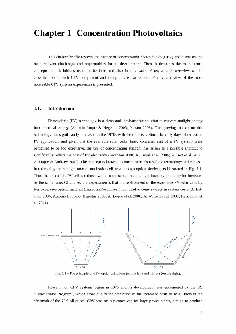
in redirecting the sunlight onto a small solar cell area through optical devices, as illustrated in Fig. 1.1.

Thus, the area of the PV cell is reduced while, at the same time, the light intensity on the device increases

by the same ratio. Of course, the expectation is that the replacement of the expensive PV solar cells by

less expensive optical material (lenses and/or mirrors) may lead to some savings in system costs (A. Bett

et al. 2006; Antonio Luque & Hegedus 2003; A. Luque et al. 2006; A. W. Bett et al. 2007; Reis, Pina, et

al. 2011).

Fig. 1.1 - The principle of CPV optics using lens (on the left) and mirrors (on the right).

Research on CPV systems began in 1975 and its development was encouraged by the US

“Concentrator Program”, which arose due to the prediction of the increased costs of fossil fuels in the

aftermath of the 70s’ oil crises. CPV was mainly conceived for large power plants, aiming to produce

4

large amounts of renewable energy and compete with conventional fossil fuel plants (A. Luque et al.

2006; Swanson 2000; A. Luque & Andreev 2007). Within this program, the first concentrator prototype

was developed at Sandia National Laboratories of Albuquerque in the mid 1976. This prototype was a

40x concentrator, making use of silicon solar cells and Fresnel lenses mounted on a two-axis tracking

system (Burgess & Pritchard 1978). Shortly afterwards, several prototypes were developed in Europe.

They were all similar to the one made by Sandia Labs.

However, the electricity market changed in a somewhat unexpected direction. Global politics

and the discovery of new oil sources kept electricity prices of the mature fossil fuel plants at a very low

level. Since the concentrator programs were initially conceived to construct CPV for large power plants,

i.e. to compete with fossil fuel generators, most of them were suspended in the face of the unexpected

abundant fossil fuel supply. This situation has slowed down the development of CPV systems. In the mid

of 1980s, R&D on concentrators faded although some groups maintained activity (A. Luque et al. 2006).

In the niche market of small remote loads used for grid extension applications (e.g. small amount

of electricity to telecommunication stations) flat-plate PV emerged as an important and viable power

source. CPV however, due to the need to be mounted on movable structures to track the sun, is

particularly unsuitable for these applications and has never gained a significant market share.

In the meantime, the new paradigm of sustainability, the need to confront global warming and

the external costs associated with pollution became the driving force for PV development. Subsidized

grid-connected market of a few kWp has emerged more recently in many developed countries. In these

applications CPV also played a minor role in PV market for more than 25 years (A. Luque et al. 2006;

Swanson 2000; A. W. Bett et al. 2007). The PV systems in the subsidized grid connected market were

often mounted on the roof or integrated in facades (reducing some of the installation cost) which again are

less suitable for CPV (A. Luque et al. 2006; Antonio Luque & Hegedus 2003; Swanson 2000; A. W. Bett

et al. 2007). However, we may found some CPV systems installed under feed-in tariff schemes in places

where extensive grounds are available (Reis, Silva, et al. 2011).

This brief historic overview emphasises the main barriers that CPV has faced when trying to

gain market acceptance. In spite of all these challenges, it should also be noticed that the development of

CPV technology has contributed to some advances in other areas. One example of such contribution is the

improvement of the efficiency of solar cells. The high power density of CPV allows the use of cells with

higher cost per unit area. Thus, many designs were developed specifically for concentration applications.

Some of these concepts have been successfully applied to one-sun solar cells (Swanson 2000).

Another technological development which has spill over from CPV to conventional PV is tracker

technology. Standard modules mounted on tracking structures may lead to higher yields that overcome

the extra cost of the trackers (Reis, Pina, et al. 2011), in particular in locations with high direct insolation.

An additional side effect of the development of CPV was the knowledge acquired about the

availability of direct normal irradiation (DNI). The boost of energy yield on CPV systems is mostly

related with the amount of direct sunlight (radiation that falls on Earth without being scattered by haze,

clouds, etc). In the early days of the Concentrator Program it was feared that the percentage of such

radiation was considerably less than the solar resource available for flat-plate systems, which make use of

global radiation. However, it was found that in many regions of good solar resource, the annual energy

5

available to a two-axis tracking concentrator is actually greater than the global radiation resource

available to flat-plate systems (Swanson 2000; Reis, Wemans, et al. 2011; Reis, Silva, et al. 2011).

During the mid 2000s, and in spite of very significant political and economic support, the cost

reduction of conventional flat plate PV was perceived to be too slow and therefore a lot of effort, and

research funding, both public and private, was re-directed to CPV, which offered the promise of a faster

learning curve. Examples are large scale CPV demonstration program in the region of Castilla La

Mancha, Spain, and in Portugal, as well as numerous start-ups dedicated to CPV that emerged in the past

5-10 years (A. Luque & Andreev 2007; Brad Hines 2007).

Today, the world is in great need of a change in the way that energy is generated. On one hand,

most governments have in their agenda the concerns about greenhouse gas emissions and climate change

while, on the other hand, the rising prices of energy and fossil fuels and the Fukushima nuclear disaster

have led to increasing interest in renewable energy sources in general, and solar in particular (Brad Hines

2007). The PV industry is now growing to a scale that it can play a measurable contribution of Europe’s

electricity mix, producing 2% of the demand in EU and roughly 4% of the peak demand (Masson et al.

2012). The character of the industry is undergoing a significant change, with abrupt cost reductions in

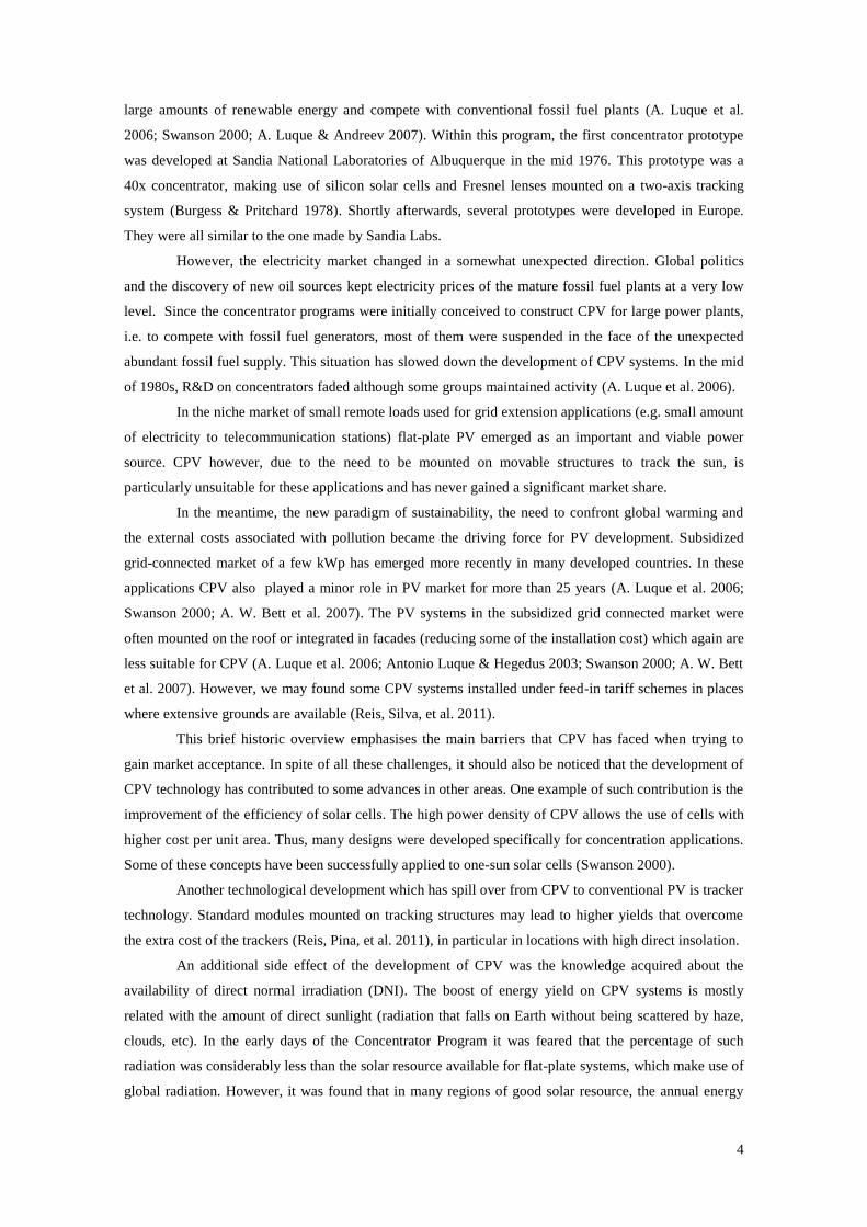
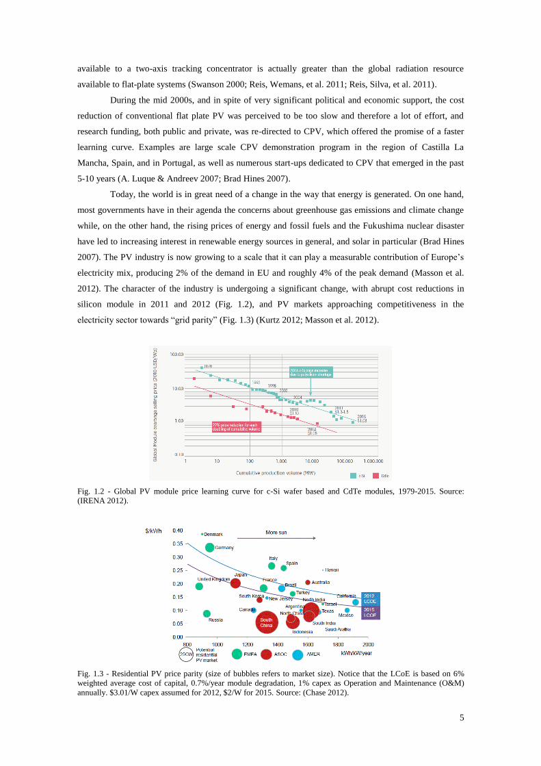
silicon module in 2011 and 2012 (Fig. 1.2), and PV markets approaching competitiveness in the

electricity sector towards “grid parity” (Fig. 1.3) (Kurtz 2012; Masson et al. 2012).

Fig. 1.2 - Global PV module price learning curve for c-Si wafer based and CdTe modules, 1979-2015. Source:

(IRENA 2012).

Fig. 1.3 - Residential PV price parity (size of bubbles refers to market size). Notice that the LCoE is based on 6%

weighted average cost of capital, 0.7%/year module degradation, 1% capex as Operation and Maintenance (O&M)

annually. $3.01/W capex assumed for 2012, $2/W for 2015. Source: (Chase 2012).

6

So the big question is how may CPV compete against traditional flat-plate PV and other

renewable energy technologies? Many factors may be pointed out (Brad Hines 2007; A. W. Bett et al.

2007; Kurtz 2012; Cameron n.d.):

Improvements in solar cell technology: solar cell manufacturers are now delivering high

efficiency solar cells above 20% for silicon and 40% for triple-junction. These high-efficient

cells are affordable for CPV systems due to the reduced area requirements. This way CPV may

achieve excellent amortization on system costs.

Desire for utility scale systems: one of the vectors that PV growth aims to reach is large

installations that yield significant power. CPV is particularly suitable for this type of applications

since large scale deployment leads to lower installation costs. In this field, CPV may have some

advantage in terms of land use since for 1 GWh uses 0.9 ha of land compared to 1.6 ha for thin-

film and 1.7 ha for a solar thermal power tower. However, this factor has only economic value in

places where land costs have a high impact on the overall system cost such as southern Europe,

Brazil or India. Still, on the path for large power plants, CPV will also compete with other

renewable energy technologies such as wind, over which has the advantage of higher

predictability and a wider selection of installations sites with much more energy available. Fossil

fuel power plants will still play a relevant role due to competitive costs; however, these plants

have a huge vulnerability to fossil fuel depletion, cost escalation and pollution directives, factors

that may lead to increased prices thus helping CPV to become competitive.

Large incentive schemes are becoming less attractive: with the increasing cost reduction on

silicon modules, incentives will become unnecessary to reach the market in a cost effective way,

in particular in sunny regions with high conventional electricity prices. This may represent a

shift on the PV market to the countries where incentive schemes are inexistent and with high

availability of sun, where CPV may be a viable option.

Relatively low capital investment: the capital investment risk for CPV is distributed between

its components (which are described in detail in the next section) and other suppliers; moreover

the cost is reduced overall because these investments may be shared to other products that use

the same materials with long-life outdoor performance demonstrated. This makes CPV

investment a lower risk than from some other types of PV.

Better match between electricity production and demand: PV systems mounted on sun

trackers, as it is almost compulsory for CPV systems, have increased production during the

mornings and afternoons, since flat plate PV are usually installed in order to optimize production

when the irradiation is higher (mid-day peak hours) ; this could be advantageous from the point

of view of the electricity grid since CPV systems may deliver power in order to fulfil demand

without the need for storage.

Concentrator leverage over traditional flat-plate systems: CPV systems have performance

advantage in sunny areas, relative lack of sensitivity to the price of solar cells, and they use less

solar cell material which may be advantageous during a time of short supply of that material.

7

Today, about 50 companies are active in the CPV technology field and almost 60% of them were

founded in the last six years (Jäger-Waldau 2012). However, in order to achieve a relevant role in the

market, the cost of CPV must be lowered. It was only recently that a number of companies started to

commercialize CPV systems (A. W. Bett et al. 2007). Most recent market estimates for 2011 in the 60

MW range, and 90 MW under construction in May 2012, the market share of CPV is still small, but

analysts forecast an increase to more than 500 MW globally by 2015 (Jäger-Waldau 2012).

Before reviewing the most noticeable CPV systems it is appropriate to briefly look over some

relevant terms, concepts and classifications in order to facilitate the understanding of the different

concepts and approaches to CPV.

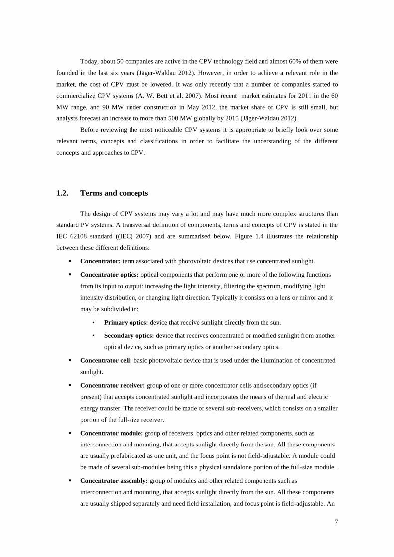
1.2. Terms and concepts

The design of CPV systems may vary a lot and may have much more complex structures than

standard PV systems. A transversal definition of components, terms and concepts of CPV is stated in the

IEC 62108 standard ((IEC) 2007) and are summarised below. Figure 1.4 illustrates the relationship

between these different definitions:

Concentrator: term associated with photovoltaic devices that use concentrated sunlight.

Concentrator optics: optical components that perform one or more of the following functions

from its input to output: increasing the light intensity, filtering the spectrum, modifying light

intensity distribution, or changing light direction. Typically it consists on a lens or mirror and it

may be subdivided in:

• Primary optics: device that receive sunlight directly from the sun.

• Secondary optics: device that receives concentrated or modified sunlight from another

optical device, such as primary optics or another secondary optics.

Concentrator cell: basic photovoltaic device that is used under the illumination of concentrated

sunlight.

Concentrator receiver: group of one or more concentrator cells and secondary optics (if

present) that accepts concentrated sunlight and incorporates the means of thermal and electric

energy transfer. The receiver could be made of several sub-receivers, which consists on a smaller

portion of the full-size receiver.

Concentrator module: group of receivers, optics and other related components, such as

interconnection and mounting, that accepts sunlight directly from the sun. All these components

are usually prefabricated as one unit, and the focus point is not field-adjustable. A module could

be made of several sub-modules being this a physical standalone portion of the full-size module.

Concentrator assembly: group of modules and other related components such as

interconnection and mounting, that accepts sunlight directly from the sun. All these components

are usually shipped separately and need field installation, and focus point is field-adjustable. An

8

assembly could be made of several sub-assemblies. The sub-assembly is a physical stand-alone,

smaller portion of the full-size assembly.

Fig. 1.4 - Terms used for CPV ((IEC) 2007).

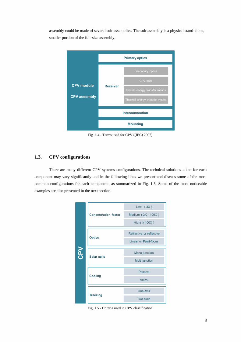
1.3. CPV configurations

There are many different CPV systems configurations. The technical solutions taken for each

component may vary significantly and in the following lines we present and discuss some of the most

common configurations for each component, as summarized in Fig. 1.5. Some of the most noticeable

examples are also presented in the next section.

Fig. 1.5 - Criteria used in CPV classification.

9

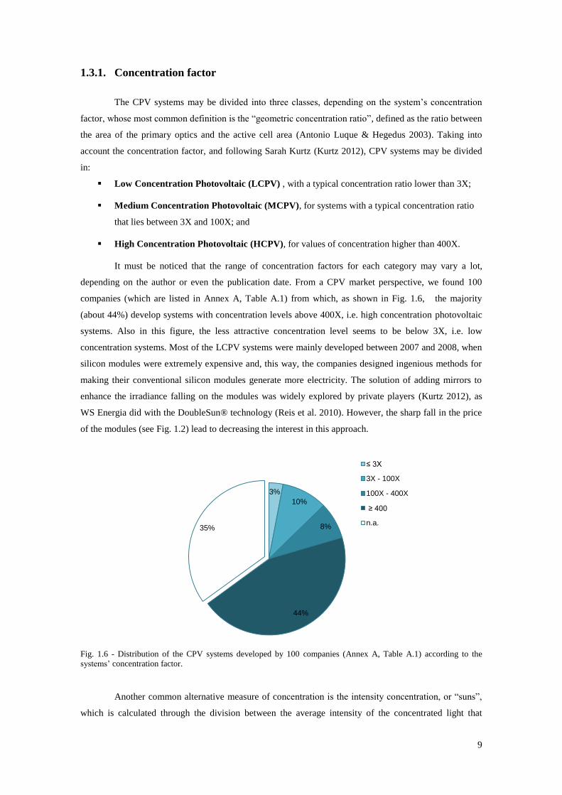
1.3.1. Concentration factor

The CPV systems may be divided into three classes, depending on the system’s concentration

factor, whose most common definition is the “geometric concentration ratio”, defined as the ratio between

the area of the primary optics and the active cell area (Antonio Luque & Hegedus 2003). Taking into

account the concentration factor, and following Sarah Kurtz (Kurtz 2012), CPV systems may be divided

in:

Low Concentration Photovoltaic (LCPV) , with a typical concentration ratio lower than 3X;

Medium Concentration Photovoltaic (MCPV), for systems with a typical concentration ratio

that lies between 3X and 100X; and

High Concentration Photovoltaic (HCPV), for values of concentration higher than 400X.

It must be noticed that the range of concentration factors for each category may vary a lot,

depending on the author or even the publication date. From a CPV market perspective, we found 100

companies (which are listed in Annex A, Table A.1) from which, as shown in Fig. 1.6, the majority

(about 44%) develop systems with concentration levels above 400X, i.e. high concentration photovoltaic

systems. Also in this figure, the less attractive concentration level seems to be below 3X, i.e. low

concentration systems. Most of the LCPV systems were mainly developed between 2007 and 2008, when

silicon modules were extremely expensive and, this way, the companies designed ingenious methods for

making their conventional silicon modules generate more electricity. The solution of adding mirrors to

enhance the irradiance falling on the modules was widely explored by private players (Kurtz 2012), as

WS Energia did with the DoubleSun® technology (Reis et al. 2010). However, the sharp fall in the price

of the modules (see Fig. 1.2) lead to decreasing the interest in this approach.

Fig. 1.6 - Distribution of the CPV systems developed by 100 companies (Annex A, Table A.1) according to the

systems’ concentration factor.

Another common alternative measure of concentration is the intensity concentration, or “suns”,

which is calculated through the division between the average intensity of the concentrated light that

3%

10%

8%

44%

35%

≤ 3X

3X - 100X

100X - 400X

≥ 400

n.a.

10

reaches the cells and the standard peak solar irradiance 1000 W/m2 (Antonio Luque & Hegedus 2003).

Both measures are valid still it should be noticed that the latter takes into account the optical losses while

the former disregard them.

1.3.2. Concentrator optics

The concentrator optics must be designed in such a way that its acceptance angle, i.e. the

maximum angle at which the rays entering the optics reach the cell, admits the misalignments and

tolerances that the manufacturing processes or tracking might introduce. The optics must be designed in

order to accept 90% of the rays coming from a cone of semi-angle , which is defined as the angular

acceptance. The optics acceptance angle must be at least the apparent sun’s semi-diameter, of 0.26° (A.

Luque et al. 2006; A. Luque & Andreev 2007).

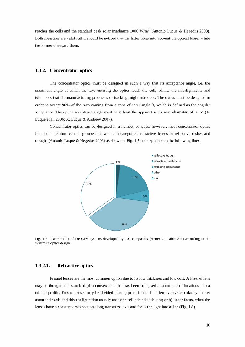
Concentrator optics can be designed in a number of ways; however, most concentrator optics

found on literature can be grouped in two main categories: refractive lenses or reflective dishes and

troughs (Antonio Luque & Hegedus 2003) as shown in Fig. 1.7 and explained in the following lines.

Fig. 1.7 - Distribution of the CPV systems developed by 100 companies (Annex A, Table A.1) according to the

systems’s optics design.

1.3.2.1. Refractive optics

Fresnel lenses are the most common option due to its low thickness and low cost. A Fresnel lens

may be thought as a standard plan convex lens that has been collapsed at a number of locations into a

thinner profile. Fresnel lenses may be divided into: a) point-focus if the lenses have circular symmetry

about their axis and this configuration usually uses one cell behind each lens; or b) linear focus, when the

lenses have a constant cross section along transverse axis and focus the light into a line (Fig. 1.8).

2%

19%

6%

38%

35%

reflective trough

refractive point-focus

reflective point-focus

other

n.a.

11

Fig. 1.8 - Fresnel lens configuration: a) point-focus lens showing a typical ray hitting the circular active area of the

solar cell; b) linear, or one-axis, lens focusing on a line of solar cells in a string; and c) domed linear lens. Source:

(Antonio Luque & Hegedus 2003).

The material of choice for the lens is usually acrylic plastic (PMMA), which moulds well and,

when combined with ultraviolet (UV) stabilizers, has shown good weatherability. However, some

disadvantages of this material should be pointed out: large thermal expansion coefficient, low strength

and stiffness, water absorption expansion and susceptibility to scratches when cleaning with any method

other than spray rinsing (Antonio Luque & Hegedus 2003).

Fresnel lenses are usually incorporated into modules that contain a lens, or multiple lenses in

parquet, a housing to protect the backside of the lens, which is difficult to clean due to the sharp facets,

and the cells. The cell may incorporate a secondary optical element (SOE) whose purpose is to further

concentrate the light or to make the image uniform. Linear Fresnel concentrators suffer severe optical

aberrations because focal distance changes with inclination of the rays with respect to the axis. This

imposes two-axis tracking on linear Fresnel systems (Antonio Luque & Hegedus 2003).

1.3.2.2. Reflective optics

A reflective surface with the shape of a parabola will focus all light parallel to the parabola’s

axis to a point located at the parabola’s focus (Antonio Luque & Hegedus 2003). Like lenses, parabolas

(Fig. 1.9) could be grouped as: i) point-focus, which is formed by rotating the parabola around its axis and

creating a paraboloid; or line focus: which is formed by translating the parabola perpendicular to its axis.

Another design option is the compound parabolic concentrator (CPC) (Oliveira et al. 1995), which typical

configuration is sketched in Fig. 1.10. The CPC is a class of concentrator called “ideal”, since it provides

the maximum possible concentration given the region of the sky it sees, or alternatively for a given

maximum acceptance angle. It is also called a “non-imaging” concentrator since the output has no

relation to the image of the sun. In spite of called ideal, CPC faces some drawbacks. First, under typical

illumination conditions, the intensity pattern at the exit aperture is relatively non-uniform. The output

12

intensity is uniform when the illumination is uniform over all directions within the acceptance angle,

which is not the case in practice since the sun provides a localized region of the sky that is much brighter

than the surrounding acceptance region (Antonio Luque & Hegedus 2003). A simplified version of this

technology uses planar reflectors and is often called a V-trough. This configuration has a maximum

intensity concentration of 3, and avoids the hot spots of the CPC (Antonio Luque & Hegedus 2003). More

details about optical performance of these systems can be found in (Martin & Ruiz 2008). For high

concentration, a CPC is rather tall and thin and thus its use is restricted to either low concentration

applications or as a secondary optical element (Antonio Luque & Hegedus 2003).

Fig. 1.9 - Reflective concentrator configurations. a) Reflective paraboloid, or dish, focusing on a cell array. b) Linear

parabolic trough focusing on a line of cells. Source: (Antonio Luque & Hegedus 2003).

Fig. 1.10 - Example of a static concentrator configuration. A bifacial cell is mounted in a reflective CPC-like trough

that is filled with liquid dielectric. Source: (Antonio Luque & Hegedus 2003).

Regarding line focus systems, they typically produce Gaussian illumination profiles, i.e. the

center of the solar cells is more illuminated than its edges (A. Luque & Andreev 2007). The impact of this

effect on the performance of the receiver will be discussed below in detail in this thesis.

Another challenge in line focus configuration arises when using single-axis tracking systems: the

end of the receiver is less illuminated than the central region and since the solar cells in the receiver are

typically connected in series, placement of bypass diodes is mandatory to avoid shaded cells to be

harmful for receiver performance (A. Luque & Andreev 2007).

13

Regarding field installation of the CPV system, the concentrator optics should withstand at least

25 years of outdoor weathering and be cleanable in order to remove accumulated dust (Antonio Luque &

Hegedus 2003).

1.3.3. Solar cells for CPV

In early designs, the solar cells integrated in CPV systems consisted of conventional silicon solar

cells or modified silicon cells for better performance under higher (more than 1 sun) irradiation levels. At

that time, multi-junction (MJ) solar cells based on III-V semiconductors, which are more efficient, were

only used in space applications since they were too expensive.

However, this perspective has changed as high and very high concentration CPV systems were

developed, which can afford these high efficiency cells without significant weight on the CPV system

total cost due to the very small cell area required (A. Luque & Andreev 2007; Kurtz 2012).

The choice of a particular solar cell technology for a given CPV application depends on how

much cost-effective it can be. Today, when considering the solar cells technology, the CPV market

systems available in the market are divided as shown in Fig. 1.11.

Fig. 1.11 - Distribution of the CPV systems developed by 100 companies (Annex A, Table A.1) according to the solar

cells technology they integrate.

Regarding solar cells efficiency, we must bear in mind that, when comparing with flat-plate PV:

CPV systems are only able to correctly collect direct radiation (which is about 80% of global

radiation in sunny regions) and

CPV optical efficiency (typically about 80%) will further decrease the efficiency of the system.

Nowadays, we may find MJ solar cells that feature very high efficiency (Fig. 1.12) but these

cells are mainly produced in small quantities by dedicated manufacturers thus having very high cost

which has inhibited their integration in low and some medium concentration systems. One should notice,

50%

21%

29%

Multi-junction

Silicon

n.a.

14

however, that silicon solar cells may be particularly competitive for these classes of concentration

systems due two main reasons:

Silicon solar cells technology has a track recorded field demonstration on terrestrial applications;

Introducing high efficiency features on standard silicon solar cell processing will increase the

cost but it will most likely still be affordable when integrated in CPV systems. Benefiting from

economies of scale this may lead to spill over to standard PV modules technologies, which will

decrease the price and increase its competitiveness for CPV application.

Fig. 1.12 - Efficiency evolution of the best research cells worldwide from 1976 up top 2012 by technology type.

Efficiencies determined by certified agencies/laboratories. Source: (L.L. Kazmerski 2012)

In this work we focus on high efficiency silicon solar cells since, as it will be discussed, this is

the technology that better meets the needs of the HSun concept, the research project within which this

research is carried out. There are different high efficiency silicon solar cells technologies suitable for

CPV application. In Chapter 2, Section 2.2.3, the Laser Grooved Buried Contact (LGBC) concept will be

discussed in detail. The following subsections present other relevant concepts worth mentioning in this

context.

1.3.3.1. Point-contact solar cells

This solar cell structure was firstly developed by Swanson and co-workers at Standford

University (A. Sinton & M. Swanson 1987). It can operate at higher concentration and has reached

efficiencies of more than 26% under concentrated light. The absence of grid on the front face allows a

better efficiency and all the electric contacts are made on the rear face through interdigitated dense grids

(Fig. 1.13). Thus, series resistance is no longer a limit for high concentration efficiency. Instead, the high

concentration efficiency is affected by the Auger recombination (A. Luque et al. 2006). From 2003,

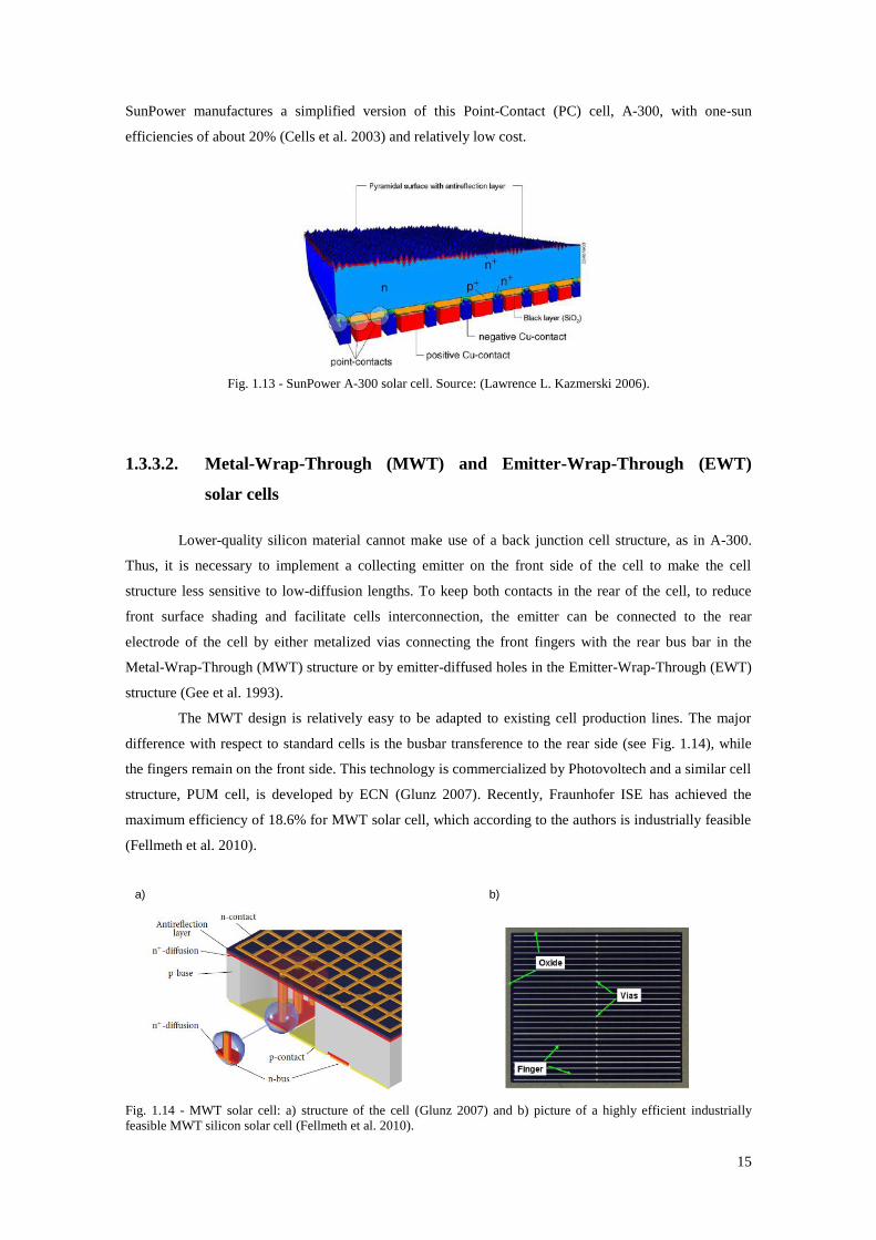
15

SunPower manufactures a simplified version of this Point-Contact (PC) cell, A-300, with one-sun

efficiencies of about 20% (Cells et al. 2003) and relatively low cost.

Fig. 1.13 - SunPower A-300 solar cell. Source: (Lawrence L. Kazmerski 2006).

1.3.3.2. Metal-Wrap-Through (MWT) and Emitter-Wrap-Through (EWT)

solar cells

Lower-quality silicon material cannot make use of a back junction cell structure, as in A-300.

Thus, it is necessary to implement a collecting emitter on the front side of the cell to make the cell

structure less sensitive to low-diffusion lengths. To keep both contacts in the rear of the cell, to reduce

front surface shading and facilitate cells interconnection, the emitter can be connected to the rear

electrode of the cell by either metalized vias connecting the front fingers with the rear bus bar in the

Metal-Wrap-Through (MWT) structure or by emitter-diffused holes in the Emitter-Wrap-Through (EWT)

structure (Gee et al. 1993).

The MWT design is relatively easy to be adapted to existing cell production lines. The major

difference with respect to standard cells is the busbar transference to the rear side (see Fig. 1.14), while

the fingers remain on the front side. This technology is commercialized by Photovoltech and a similar cell

structure, PUM cell, is developed by ECN (Glunz 2007). Recently, Fraunhofer ISE has achieved the

maximum efficiency of 18.6% for MWT solar cell, which according to the authors is industrially feasible

(Fellmeth et al. 2010).

a)

b)

Fig. 1.14 - MWT solar cell: a) structure of the cell (Glunz 2007) and b) picture of a highly efficient industrially

feasible MWT silicon solar cell (Fellmeth et al. 2010).

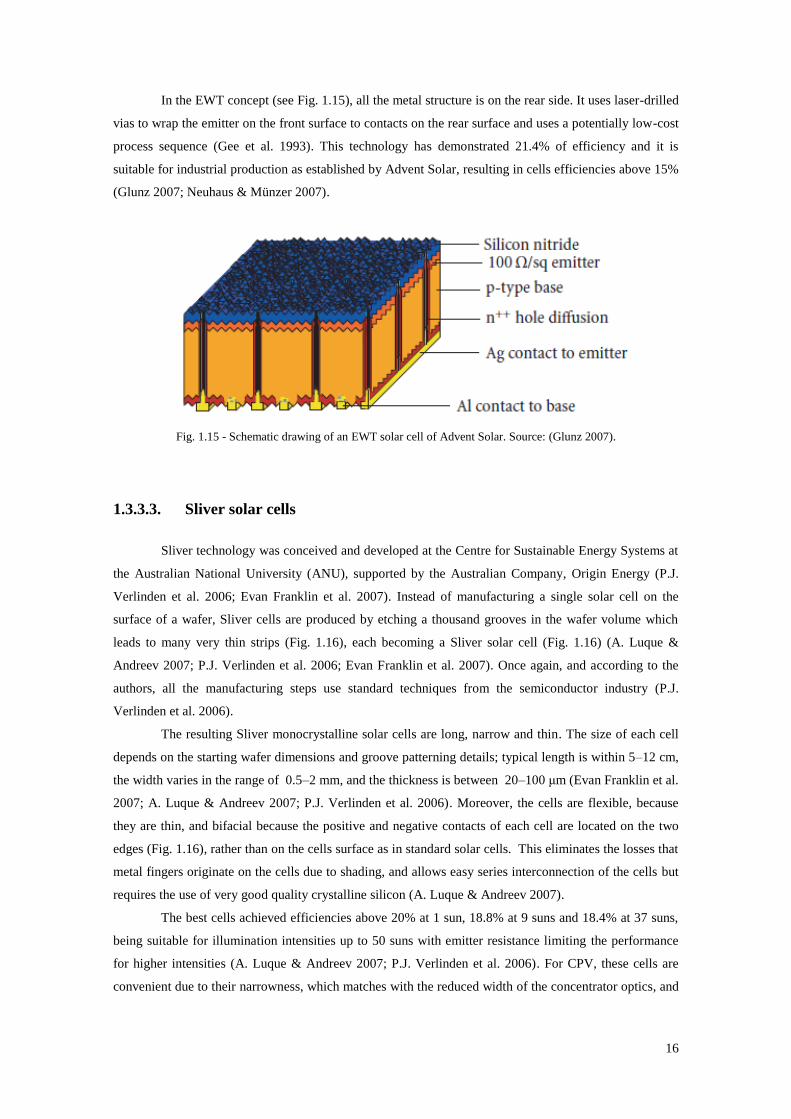
16

In the EWT concept (see Fig. 1.15), all the metal structure is on the rear side. It uses laser-drilled

vias to wrap the emitter on the front surface to contacts on the rear surface and uses a potentially low-cost

process sequence (Gee et al. 1993). This technology has demonstrated 21.4% of efficiency and it is

suitable for industrial production as established by Advent Solar, resulting in cells efficiencies above 15%

(Glunz 2007; Neuhaus & Münzer 2007).

Fig. 1.15 - Schematic drawing of an EWT solar cell of Advent Solar. Source: (Glunz 2007).

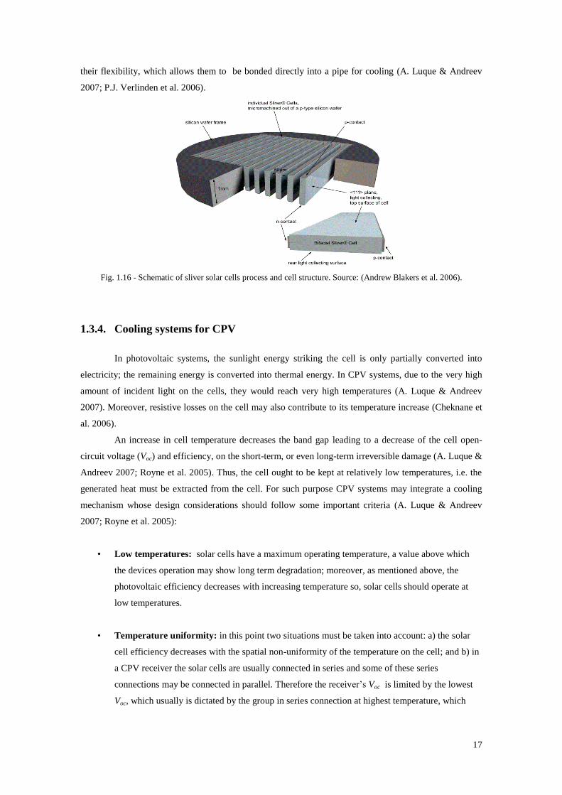
1.3.3.3. Sliver solar cells

Sliver technology was conceived and developed at the Centre for Sustainable Energy Systems at

the Australian National University (ANU), supported by the Australian Company, Origin Energy (P.J.

Verlinden et al. 2006; Evan Franklin et al. 2007). Instead of manufacturing a single solar cell on the

surface of a wafer, Sliver cells are produced by etching a thousand grooves in the wafer volume which

leads to many very thin strips (Fig. 1.16), each becoming a Sliver solar cell (Fig. 1.16) (A. Luque &

Andreev 2007; P.J. Verlinden et al. 2006; Evan Franklin et al. 2007). Once again, and according to the

authors, all the manufacturing steps use standard techniques from the semiconductor industry (P.J.

Verlinden et al. 2006).

The resulting Sliver monocrystalline solar cells are long, narrow and thin. The size of each cell

depends on the starting wafer dimensions and groove patterning details; typical length is within 5–12 cm,

the width varies in the range of 0.5–2 mm, and the thickness is between 20–100 μm (Evan Franklin et al.

2007; A. Luque & Andreev 2007; P.J. Verlinden et al. 2006). Moreover, the cells are flexible, because

they are thin, and bifacial because the positive and negative contacts of each cell are located on the two

edges (Fig. 1.16), rather than on the cells surface as in standard solar cells. This eliminates the losses that

metal fingers originate on the cells due to shading, and allows easy series interconnection of the cells but

requires the use of very good quality crystalline silicon (A. Luque & Andreev 2007).

The best cells achieved efficiencies above 20% at 1 sun, 18.8% at 9 suns and 18.4% at 37 suns,

being suitable for illumination intensities up to 50 suns with emitter resistance limiting the performance

for higher intensities (A. Luque & Andreev 2007; P.J. Verlinden et al. 2006). For CPV, these cells are

convenient due to their narrowness, which matches with the reduced width of the concentrator optics, and

17

their flexibility, which allows them to be bonded directly into a pipe for cooling (A. Luque & Andreev

2007; P.J. Verlinden et al. 2006).

Fig. 1.16 - Schematic of sliver solar cells process and cell structure. Source: (Andrew Blakers et al. 2006).

1.3.4. Cooling systems for CPV

In photovoltaic systems, the sunlight energy striking the cell is only partially converted into

electricity; the remaining energy is converted into thermal energy. In CPV systems, due to the very high

amount of incident light on the cells, they would reach very high temperatures (A. Luque & Andreev

2007). Moreover, resistive losses on the cell may also contribute to its temperature increase (Cheknane et

al. 2006).

An increase in cell temperature decreases the band gap leading to a decrease of the cell open-

circuit voltage (Voc) and efficiency, on the short-term, or even long-term irreversible damage (A. Luque &

Andreev 2007; Royne et al. 2005). Thus, the cell ought to be kept at relatively low temperatures, i.e. the

generated heat must be extracted from the cell. For such purpose CPV systems may integrate a cooling

mechanism whose design considerations should follow some important criteria (A. Luque & Andreev

2007; Royne et al. 2005):

• Low temperatures: solar cells have a maximum operating temperature, a value above which

the devices operation may show long term degradation; moreover, as mentioned above, the

photovoltaic efficiency decreases with increasing temperature so, solar cells should operate at

low temperatures.

• Temperature uniformity: in this point two situations must be taken into account: a) the solar

cell efficiency decreases with the spatial non-uniformity of the temperature on the cell; and b) in

a CPV receiver the solar cells are usually connected in series and some of these series

connections may be connected in parallel. Therefore the receiver’s Voc is limited by the lowest

Voc, which usually is dictated by the group in series connection at highest temperature, which

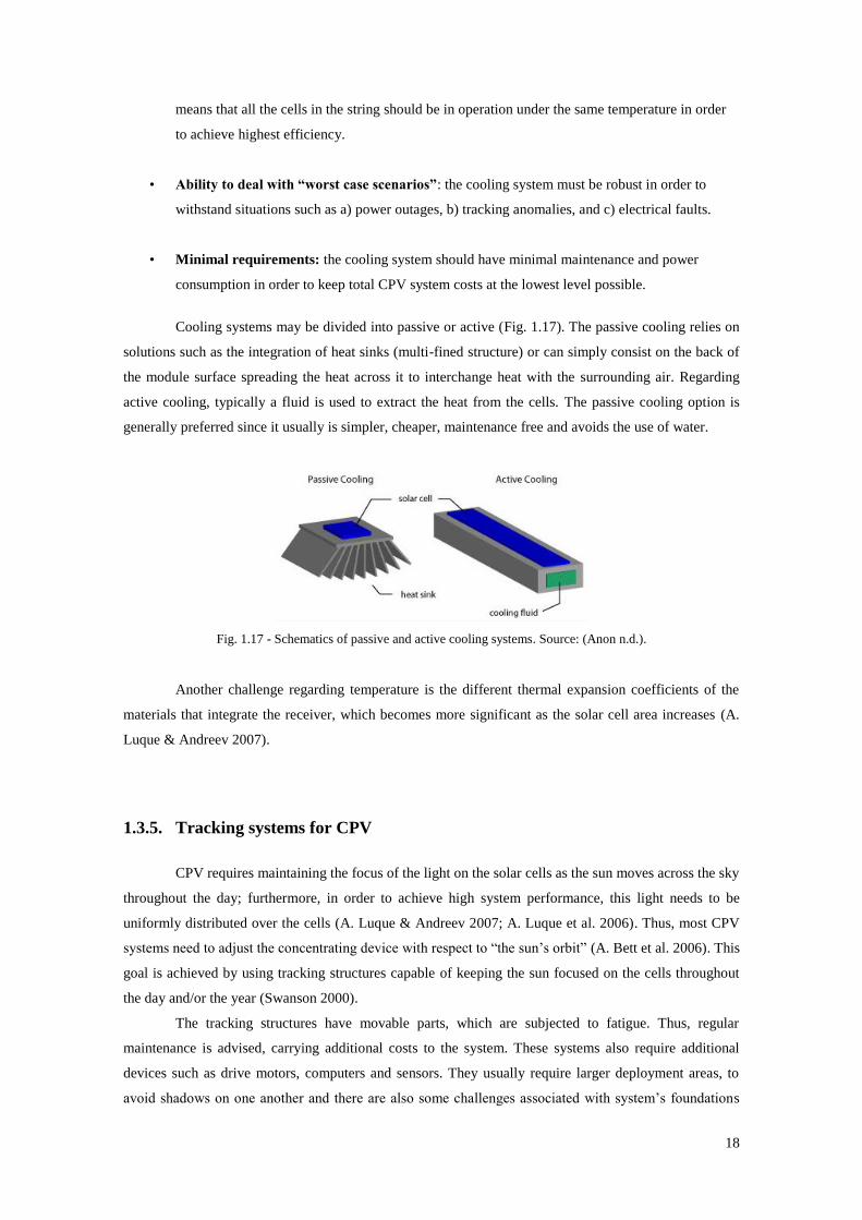
18

means that all the cells in the string should be in operation under the same temperature in order

to achieve highest efficiency.

• Ability to deal with “worst case scenarios”: the cooling system must be robust in order to

withstand situations such as a) power outages, b) tracking anomalies, and c) electrical faults.

• Minimal requirements: the cooling system should have minimal maintenance and power

consumption in order to keep total CPV system costs at the lowest level possible.

Cooling systems may be divided into passive or active (Fig. 1.17). The passive cooling relies on

solutions such as the integration of heat sinks (multi-fined structure) or can simply consist on the back of

the module surface spreading the heat across it to interchange heat with the surrounding air. Regarding

active cooling, typically a fluid is used to extract the heat from the cells. The passive cooling option is

generally preferred since it usually is simpler, cheaper, maintenance free and avoids the use of water.

Fig. 1.17 - Schematics of passive and active cooling systems. Source: (Anon n.d.).

Another challenge regarding temperature is the different thermal expansion coefficients of the

materials that integrate the receiver, which becomes more significant as the solar cell area increases (A.

Luque & Andreev 2007).

1.3.5. Tracking systems for CPV

CPV requires maintaining the focus of the light on the solar cells as the sun moves across the sky

throughout the day; furthermore, in order to achieve high system performance, this light needs to be

uniformly distributed over the cells (A. Luque & Andreev 2007; A. Luque et al. 2006). Thus, most CPV

systems need to adjust the concentrating device with respect to “the sun’s orbit” (A. Bett et al. 2006). This

goal is achieved by using tracking structures capable of keeping the sun focused on the cells throughout

the day and/or the year (Swanson 2000).

The tracking structures have movable parts, which are subjected to fatigue. Thus, regular

maintenance is advised, carrying additional costs to the system. These systems also require additional

devices such as drive motors, computers and sensors. They usually require larger deployment areas, to

avoid shadows on one another and there are also some challenges associated with system’s foundations

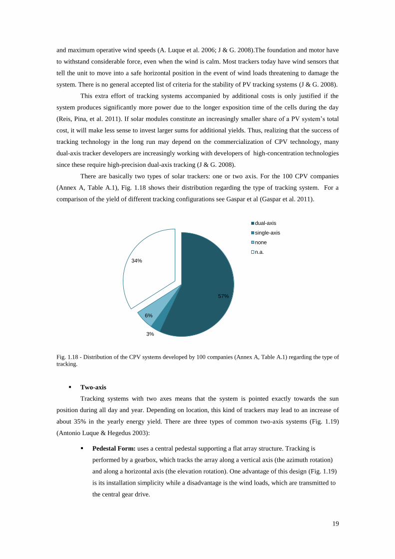
19

and maximum operative wind speeds (A. Luque et al. 2006; J & G. 2008).The foundation and motor have

to withstand considerable force, even when the wind is calm. Most trackers today have wind sensors that

tell the unit to move into a safe horizontal position in the event of wind loads threatening to damage the

system. There is no general accepted list of criteria for the stability of PV tracking systems (J & G. 2008).

This extra effort of tracking systems accompanied by additional costs is only justified if the

system produces significantly more power due to the longer exposition time of the cells during the day

(Reis, Pina, et al. 2011). If solar modules constitute an increasingly smaller share of a PV system’s total

cost, it will make less sense to invest larger sums for additional yields. Thus, realizing that the success of

tracking technology in the long run may depend on the commercialization of CPV technology, many

dual-axis tracker developers are increasingly working with developers of high-concentration technologies

since these require high-precision dual-axis tracking (J & G. 2008).

There are basically two types of solar trackers: one or two axis. For the 100 CPV companies

(Annex A, Table A.1), Fig. 1.18 shows their distribution regarding the type of tracking system. For a

comparison of the yield of different tracking configurations see Gaspar et al (Gaspar et al. 2011).

Fig. 1.18 - Distribution of the CPV systems developed by 100 companies (Annex A, Table A.1) regarding the type of

tracking.

Two-axis

Tracking systems with two axes means that the system is pointed exactly towards the sun

position during all day and year. Depending on location, this kind of trackers may lead to an increase of

about 35% in the yearly energy yield. There are three types of common two-axis systems (Fig. 1.19)

(Antonio Luque & Hegedus 2003):

Pedestal Form: uses a central pedestal supporting a flat array structure. Tracking is

performed by a gearbox, which tracks the array along a vertical axis (the azimuth rotation)

and along a horizontal axis (the elevation rotation). One advantage of this design (Fig. 1.19)

is its installation simplicity while a disadvantage is the wind loads, which are transmitted to

the central gear drive.

57%

3%

6%

34%

dual-axis

single-axis

none

n.a.

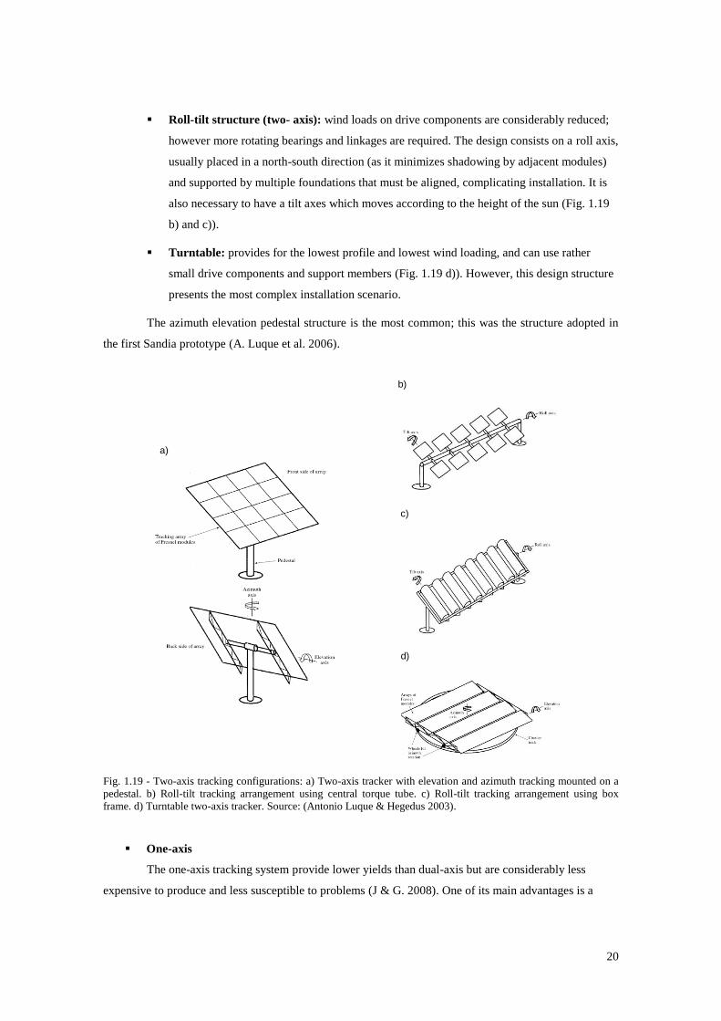
20

Roll-tilt structure (two- axis): wind loads on drive components are considerably reduced;

however more rotating bearings and linkages are required. The design consists on a roll axis,

usually placed in a north-south direction (as it minimizes shadowing by adjacent modules)

and supported by multiple foundations that must be aligned, complicating installation. It is

also necessary to have a tilt axes which moves according to the height of the sun (Fig. 1.19

b) and c)).

Turntable: provides for the lowest profile and lowest wind loading, and can use rather

small drive components and support members (Fig. 1.19 d)). However, this design structure

presents the most complex installation scenario.

The azimuth elevation pedestal structure is the most common; this was the structure adopted in

the first Sandia prototype (A. Luque et al. 2006).

a)

b)

c)

d)

Fig. 1.19 - Two-axis tracking configurations: a) Two-axis tracker with elevation and azimuth tracking mounted on a

pedestal. b) Roll-tilt tracking arrangement using central torque tube. c) Roll-tilt tracking arrangement using box

frame. d) Turntable two-axis tracker. Source: (Antonio Luque & Hegedus 2003).

One-axis

The one-axis tracking system provide lower yields than dual-axis but are considerably less

expensive to produce and less susceptible to problems (J & G. 2008). One of its main advantages is a

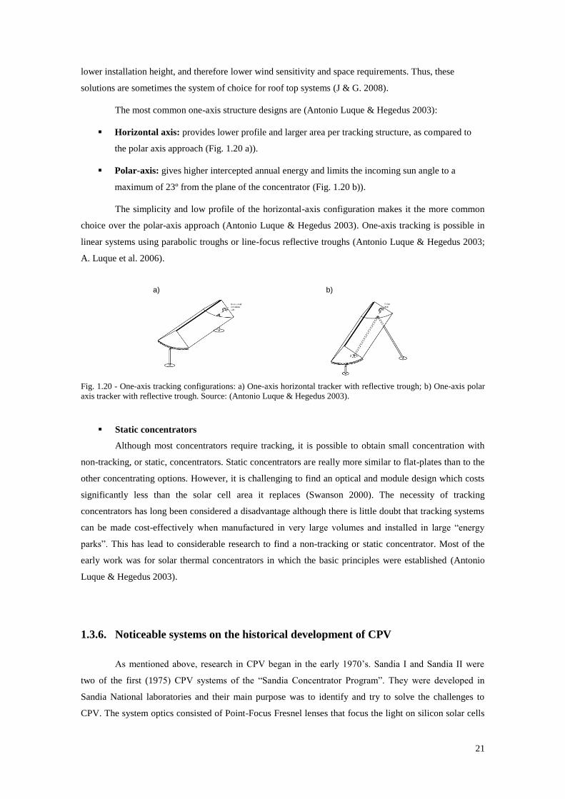
21

lower installation height, and therefore lower wind sensitivity and space requirements. Thus, these

solutions are sometimes the system of choice for roof top systems (J & G. 2008).

The most common one-axis structure designs are (Antonio Luque & Hegedus 2003):

Horizontal axis: provides lower profile and larger area per tracking structure, as compared to

the polar axis approach (Fig. 1.20 a)).

Polar-axis: gives higher intercepted annual energy and limits the incoming sun angle to a

maximum of 23º from the plane of the concentrator (Fig. 1.20 b)).

The simplicity and low profile of the horizontal-axis configuration makes it the more common

choice over the polar-axis approach (Antonio Luque & Hegedus 2003). One-axis tracking is possible in

linear systems using parabolic troughs or line-focus reflective troughs (Antonio Luque & Hegedus 2003;

A. Luque et al. 2006).

a)

b)

Fig. 1.20 - One-axis tracking configurations: a) One-axis horizontal tracker with reflective trough; b) One-axis polar

axis tracker with reflective trough. Source: (Antonio Luque & Hegedus 2003).

Static concentrators

Although most concentrators require tracking, it is possible to obtain small concentration with

non-tracking, or static, concentrators. Static concentrators are really more similar to flat-plates than to the

other concentrating options. However, it is challenging to find an optical and module design which costs

significantly less than the solar cell area it replaces (Swanson 2000). The necessity of tracking

concentrators has long been considered a disadvantage although there is little doubt that tracking systems

can be made cost-effectively when manufactured in very large volumes and installed in large “energy

parks”. This has lead to considerable research to find a non-tracking or static concentrator. Most of the

early work was for solar thermal concentrators in which the basic principles were established (Antonio

Luque & Hegedus 2003).

1.3.6. Noticeable systems on the historical development of CPV

As mentioned above, research in CPV began in the early 1970’s. Sandia I and Sandia II were

two of the first (1975) CPV systems of the “Sandia Concentrator Program”. They were developed in

Sandia National laboratories and their main purpose was to identify and try to solve the challenges to

CPV. The system optics consisted of Point-Focus Fresnel lenses that focus the light on silicon solar cells

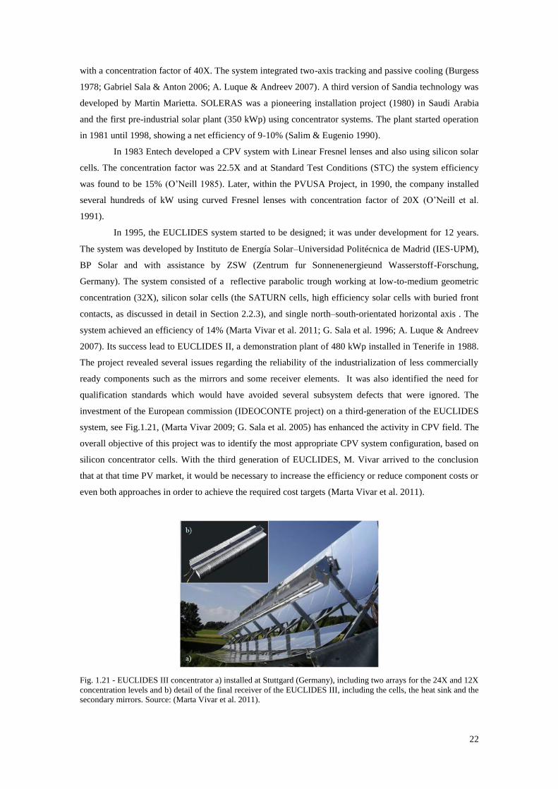
22

with a concentration factor of 40X. The system integrated two-axis tracking and passive cooling (Burgess

1978; Gabriel Sala & Anton 2006; A. Luque & Andreev 2007). A third version of Sandia technology was

developed by Martin Marietta. SOLERAS was a pioneering installation project (1980) in Saudi Arabia

and the first pre-industrial solar plant (350 kWp) using concentrator systems. The plant started operation

in 1981 until 1998, showing a net efficiency of 9-10% (Salim & Eugenio 1990).

In 1983 Entech developed a CPV system with Linear Fresnel lenses and also using silicon solar

cells. The concentration factor was 22.5X and at Standard Test Conditions (STC) the system efficiency

was found to be 15% (O’Neill 1985). Later, within the PVUSA Project, in 1990, the company installed

several hundreds of kW using curved Fresnel lenses with concentration factor of 20X (O’Neill et al.

1991).

In 1995, the EUCLIDES system started to be designed; it was under development for 12 years.

The system was developed by Instituto de Energía Solar–Universidad Politécnica de Madrid (IES‐UPM),

BP Solar and with assistance by ZSW (Zentrum fur Sonnenenergieund Wasserstoff-Forschung,

Germany). The system consisted of a reflective parabolic trough working at low-to-medium geometric

concentration (32X), silicon solar cells (the SATURN cells, high efficiency solar cells with buried front

contacts, as discussed in detail in Section 2.2.3), and single north–south‐orientated horizontal axis . The

system achieved an efficiency of 14% (Marta Vivar et al. 2011; G. Sala et al. 1996; A. Luque & Andreev

2007). Its success lead to EUCLIDES II, a demonstration plant of 480 kWp installed in Tenerife in 1988.

The project revealed several issues regarding the reliability of the industrialization of less commercially

ready components such as the mirrors and some receiver elements. It was also identified the need for

qualification standards which would have avoided several subsystem defects that were ignored. The

investment of the European commission (IDEOCONTE project) on a third-generation of the EUCLIDES

system, see Fig.1.21, (Marta Vivar 2009; G. Sala et al. 2005) has enhanced the activity in CPV field. The

overall objective of this project was to identify the most appropriate CPV system configuration, based on

silicon concentrator cells. With the third generation of EUCLIDES, M. Vivar arrived to the conclusion

that at that time PV market, it would be necessary to increase the efficiency or reduce component costs or

even both approaches in order to achieve the required cost targets (Marta Vivar et al. 2011).

Fig. 1.21 - EUCLIDES III concentrator a) installed at Stuttgard (Germany), including two arrays for the 24X and 12X

concentration levels and b) detail of the final receiver of the EUCLIDES III, including the cells, the heat sink and the

secondary mirrors. Source: (Marta Vivar et al. 2011).

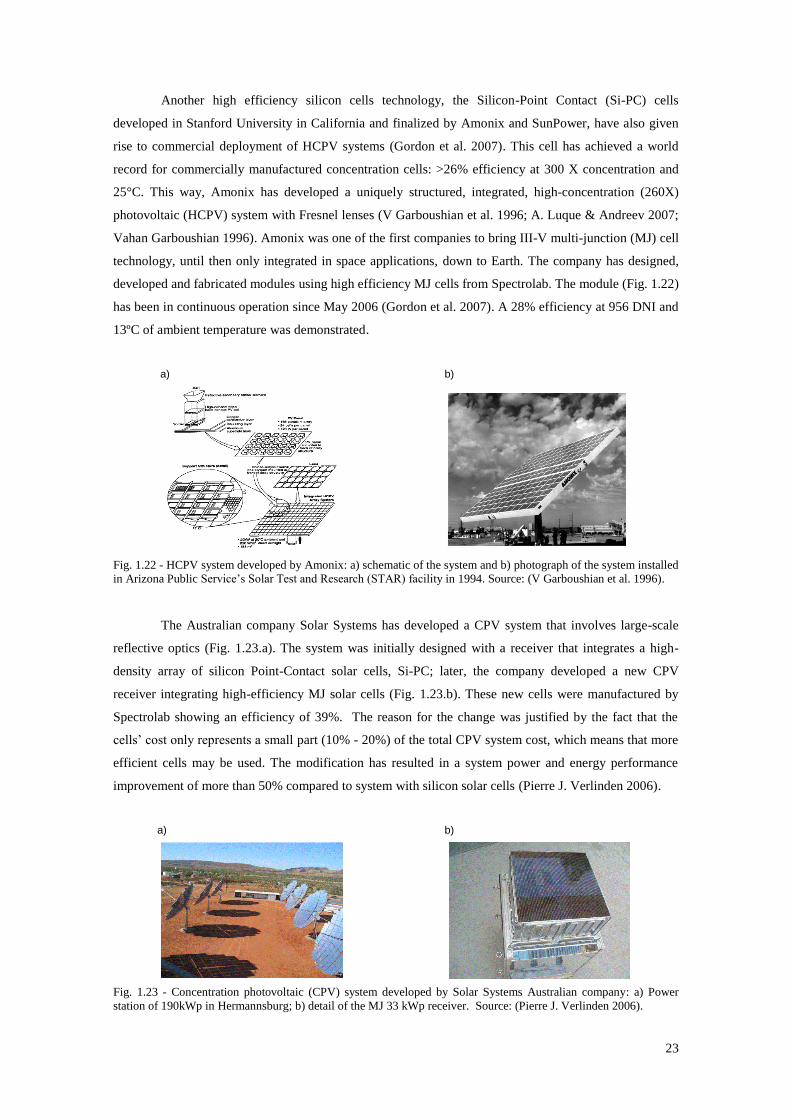
23

Another high efficiency silicon cells technology, the Silicon-Point Contact (Si-PC) cells

developed in Stanford University in California and finalized by Amonix and SunPower, have also given

rise to commercial deployment of HCPV systems (Gordon et al. 2007). This cell has achieved a world

record for commercially manufactured concentration cells: >26% efficiency at 300 X concentration and

25°C. This way, Amonix has developed a uniquely structured, integrated, high-concentration (260X)

photovoltaic (HCPV) system with Fresnel lenses (V Garboushian et al. 1996; A. Luque & Andreev 2007;

Vahan Garboushian 1996). Amonix was one of the first companies to bring III-V multi-junction (MJ) cell

technology, until then only integrated in space applications, down to Earth. The company has designed,

developed and fabricated modules using high efficiency MJ cells from Spectrolab. The module (Fig. 1.22)

has been in continuous operation since May 2006 (Gordon et al. 2007). A 28% efficiency at 956 DNI and

13ºC of ambient temperature was demonstrated.

a) b)

Fig. 1.22 - HCPV system developed by Amonix: a) schematic of the system and b) photograph of the system installed

in Arizona Public Service’s Solar Test and Research (STAR) facility in 1994. Source: (V Garboushian et al. 1996).

The Australian company Solar Systems has developed a CPV system that involves large-scale

reflective optics (Fig. 1.23.a). The system was initially designed with a receiver that integrates a high-

density array of silicon Point-Contact solar cells, Si-PC; later, the company developed a new CPV

receiver integrating high-efficiency MJ solar cells (Fig. 1.23.b). These new cells were manufactured by

Spectrolab showing an efficiency of 39%. The reason for the change was justified by the fact that the

cells’ cost only represents a small part (10% - 20%) of the total CPV system cost, which means that more

efficient cells may be used. The modification has resulted in a system power and energy performance

improvement of more than 50% compared to system with silicon solar cells (Pierre J. Verlinden 2006).

a) b)

Fig. 1.23 - Concentration photovoltaic (CPV) system developed by Solar Systems Australian company: a) Power

station of 190kWp in Hermannsburg; b) detail of the MJ 33 kWp receiver. Source: (Pierre J. Verlinden 2006).

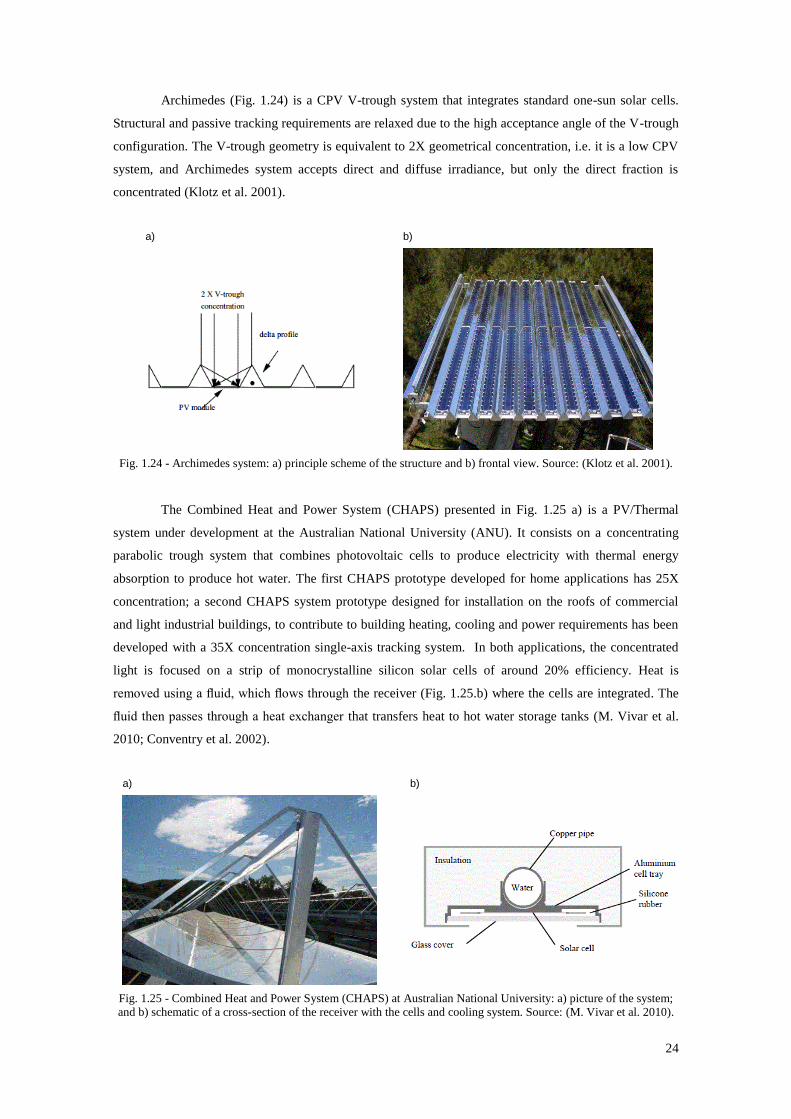
24

Archimedes (Fig. 1.24) is a CPV V-trough system that integrates standard one-sun solar cells.

Structural and passive tracking requirements are relaxed due to the high acceptance angle of the V-trough

configuration. The V-trough geometry is equivalent to 2X geometrical concentration, i.e. it is a low CPV

system, and Archimedes system accepts direct and diffuse irradiance, but only the direct fraction is

concentrated (Klotz et al. 2001).

a) b)

Fig. 1.24 - Archimedes system: a) principle scheme of the structure and b) frontal view. Source: (Klotz et al. 2001).

The Combined Heat and Power System (CHAPS) presented in Fig. 1.25 a) is a PV/Thermal

system under development at the Australian National University (ANU). It consists on a concentrating

parabolic trough system that combines photovoltaic cells to produce electricity with thermal energy

absorption to produce hot water. The first CHAPS prototype developed for home applications has 25X

concentration; a second CHAPS system prototype designed for installation on the roofs of commercial

and light industrial buildings, to contribute to building heating, cooling and power requirements has been

developed with a 35X concentration single-axis tracking system. In both applications, the concentrated

light is focused on a strip of monocrystalline silicon solar cells of around 20% efficiency. Heat is

removed using a fluid, which flows through the receiver (Fig. 1.25.b) where the cells are integrated. The

fluid then passes through a heat exchanger that transfers heat to hot water storage tanks (M. Vivar et al.

2010; Conventry et al. 2002).

a) b)

Fig. 1.25 - Combined Heat and Power System (CHAPS) at Australian National University: a) picture of the system;

and b) schematic of a cross-section of the receiver with the cells and cooling system. Source: (M. Vivar et al. 2010).

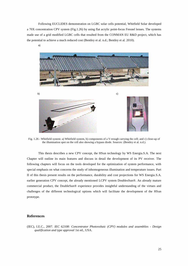
25

Following EUCLIDES demonstration on LGBC solar cells potential, Whitfield Solar developed

a 70X concentration CPV system (Fig.1.26) by using flat acrylic point-focus Fresnel lenses. The systems

made use of a grid modified LGBC cells that resulted from the CONMAN EU R&D project, which has

the potential to achieve a much reduced cost (Bentley et al. n.d.; Bentley et al. 2010).

a)

b) c)

Fig. 1.26 - Whitfield system: a) Whitfield system, b) components of a V-trough carrying the cell; and c) close-up of

the illumination spot on the cell also showing a bypass diode. Sources: (Bentley et al. n.d.).

This thesis describes a new CPV concept, the HSun technology by WS Energia.S.A. The next

Chapter will outline its main features and discuss in detail the development of its PV receiver. The

following chapters will focus on the tools developed for the optimization of system performance, with

special emphasis on what concerns the study of inhomogeneous illumination and temperature issues. Part

II of this thesis present results on the performance, durability and cost projections for WS Energia.S.A.

earlier generation CPV concept, the already mentioned LCPV system DoublesSun®. An already mature

commercial product, the DoubleSun® experience provides insightful understanding of the virtues and

challenges of the different technological options which will facilitate the development of the HSun

prototype.

References

(IEC), I.E.C., 2007. IEC 62108: Concentrator Photovoltaic (CPV) modules and assemblies - Design

qualification and type approval 1st ed., USA.

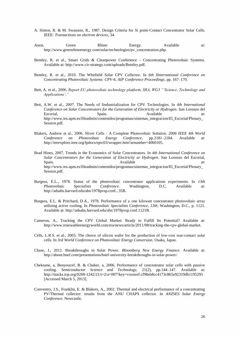
26

A. Sinton, R. & M. Swanson, R., 1987. Design Criteria for Si point-Contact Concentrator Solar Cells.

IEEE: Transactions on electron devices, 34.

Anon, Green Rhino Energy. Available at:

http://www.greenrhinoenergy.com/solar/technologies/pv_concentration.php.

Bentley, R. et al., Smart Grids & Cleanpower Conference - Concentrating Photovoltaic Systems.

Available at: http://www.cir-strategy.com/uploads/Bentley.pdf.

Bentley, R. et al., 2010. The Whitfield Solar CPV Collector. In 6th IInternational Conference on

Concentrating Photovoltaic Systems: CPV-6. AIP Conference Proceedings. pp. 167–170.

Bett, A. et al., 2006. Report EU photovoltaic technology platform, SRA, WG3 “‘Science, Technology and

Applications’,”

Bett, A.W. et al., 2007. The Needs of Iindustrialization for CPV Technologies. In 4th International

Conference on Solar Concentrators for the Generation of Electricity or Hydrogen. San Lorenzo del

Escorial, Spain. Available at:

http://www.ies.upm.es/fileadmin/contenidos/programas/sistemas_integracion/El_Escorial/Plenary_

Session.pdf.

Blakers, Andrew et al., 2006. Sliver Cells - A Complete Photovoltaic Solution. 2006 IEEE 4th World

Conference on Photovoltaic Energy Conference, pp.2181–2184. Available at:

http://ieeexplore.ieee.org/lpdocs/epic03/wrapper.htm?arnumber=4060105.

Brad Hines, 2007. Trends in the Economics of Solar Concentrators. In 4th International Conference on

Solar Concentrators for the Generation of Electricity or Hydrogen. San Lorenzo del Escorial,

Spain. Available at:

http://www.ies.upm.es/fileadmin/contenidos/programas/sistemas_integracion/El_Escorial/Plenary_

Session.pdf.

Burgess, E.L., 1978. Status of the photovoltaic concentrator applications experiments. In 13th

Photovoltaic Specialists Conference. Washington, D.C. Available at:

http://adsabs.harvard.edu/abs/1978pvsp.conf...35B.

Burgess, E.L. & Pritchard, D.A., 1978. Performance of a one kilowatt concentrator photovoltaic array

utilizing active cooling. In Photovoltaic Specialists Conference, 13th. Washington, D.C., p. 1121.

Available at: http://adsabs.harvard.edu/abs/1978pvsp.conf.1121B.

Cameron, A., Tracking the CPV Global Market: Ready to Fulfill Its Potential? Available at:

http://www.renewableenergyworld.com/rea/news/article/2011/08/tracking-the-cpv-global-market.

Cells, L.R.S. et al., 2003. The choice of silicon wafer for the production of low-cost rear-contact solar

cells. In 3rd World Conference on Photovoltaic Energy Conversion. Osaka, Japan.

Chase, J., 2012. Breakthroughs in Solar Power. Bloomberg New Energy Finance. Available at:

http://about.bnef.com/presentations/bnef-university-breakthroughs-in-solar-power/.

Cheknane, a, Benyoucef, B. & Chaker, a, 2006. Performance of concentrator solar cells with passive

cooling. Semiconductor Science and Technology, 21(2), pp.144–147. Available at:

http://stacks.iop.org/0268-1242/21/i=2/a=007?key=crossref.cf98eb8cc4173c865e92319db1195295

[Accessed March 5, 2013].

Conventry, J.S., Franklin, E. & Blakers, A., 2002. Thermal and electrical performance of a concentrating

PV/Thermal collector: results from the ANU CHAPS collector. In ANZSES Solar Energy

Conference. Newcastle.

27

Fellmeth, T. et al., 2010. Highly efficient industrially feasible metal wrap through (MWT) silicon solar

cells. Solar Energy Materials and Solar Cells, 94(12), pp.1996–2001. Available at:

http://linkinghub.elsevier.com/retrieve/pii/S0927024810004629 [Accessed March 1, 2013].

Franklin, Evan et al., 2007. Sliver Solar Cells: High-Efficiency, Low-Cost PV Technology. Advances in

OptoElectronics, 2007, pp.1–9. Available at:

http://www.hindawi.com/journals/aoe/2007/035383/abs/ [Accessed March 6, 2013].

Garboushian, V et al., 1996. An Evaluation of Integrated High-Concentration Photovoltaics for Large-

scale Grid Connected Applications. In Photovoltaic Specialists Conference, 1996., Conference

Record of the Twenty Fifth IEEE. pp. 1373 – 1376.

Garboushian, Vahan, 1996. Development of back junction point contact photovoltaic cells and arrays for

space. In Photovoltaic Specialists Conference, Conference Record of the Twenty Fifth IEEE. pp.

227 – 230.

Gaspar, G. et al., 2011. Exploring One-Axis Tracking Configurations For CPV Application. In 7th

International Conference on Concentrating Photovoltaic Systems: CPV-7. AIP Conference

Proceedings.

Gee, J.M., Schubert, W.K. & Basore, P. a., 1993. Emitter wrap-through solar cell. Conference Record of

the Twenty Third IEEE Photovoltaic Specialists Conference - 1993 (Cat. No.93CH3283-9), pp.265–

270. Available at: http://ieeexplore.ieee.org/lpdocs/epic03/wrapper.htm?arnumber=347173.

Glunz, S.W., 2007. High-Efficiency Crystalline Silicon Solar Cells. Advances in OptoElectronics,

2007(i), pp.1–15. Available at: http://www.hindawi.com/journals/aoe/2007/097370/abs/ [Accessed

March 6, 2013].

Gordon, R., Slade, A. & Garboushian, Vahan, 2007. A 30% efficient (>250 Watt) module using

multijunction solar cells and their one-year on-sun field performance. M. Symko-Davies, ed. ,

pp.664902–664902–9. Available at:

http://proceedings.spiedigitallibrary.org/proceeding.aspx?doi=10.1117/12.732700.

IRENA, 2012. Renewable Energy Tecnologies: Cost Analysis Series - Solar Photovoltaics. , 1(4).

J, S. & G., H., 2008. Gearing up for a price war. In: The market for tracking systems is entering a new

phase: that of uncompromising optimization. Photon International;

Jäger-Waldau, A., 2012. JRC Scientificand Policy Reports - PV Status Report 2012, Ispra, Italy.

Kazmerski, L.L., 2012. Best Research - Cell Efficiencies. National Renewable Energy Laboratory

(NREL), Golden, CO. Available at: http://en.wikipedia.org/wiki/File:PVeff(rev120404).jpg.

Kazmerski, Lawrence L., 2006. Solar photovoltaics R&D at the tipping point: A 2005 technology

overview. Journal of Electron Spectroscopy and Related Phenomena, 150(2-3), pp.105–135.

Available at: http://linkinghub.elsevier.com/retrieve/pii/S0368204805004615 [Accessed March 6,

2013].

Klotz, F.H. et al., 2001. Field test results of the Archimedes photovoltaic V-trough concentrator systems.

In Proceedings of the 17th European Photovoltaic Solar Energy Conference and Exhibition.

Munich, Germany, pp. 492–495.

Kurtz, S., 2012. Opportunities and Challenges for Development of a Mature Concentrating Photovoltaic

Power Industry, Colorado.

Luque, A. & Andreev, V. eds., 2007. Concentrator Photovoltaics, Springer.

28

Luque, A., Sala, G. & Luque-Heredia, I., 2006. Photovoltaic Concentration at the Onset of its

Commercial Deployment. Progress in Photovoltaics: Research and Applications, (14), pp.413–428.

Available at: http://onlinelibrary.wiley.com/doi/10.1002/pip.705/pdf.

Luque, Antonio & Hegedus, S. eds., 2003. Handbook of Photovoltaic Science and Engineering 1st ed.,

John Wiley & Sons Ltd.

Martin, N. & Ruiz, J., 2008. Optical performance analysis of V-trough PV concentrators. Progress in

Photovoltaics: Research and Applications, 16, pp.339–348. Available at:

http://www.appropedia.org/Low_level_concentration_for_PV_applications#N._Mart.C3.ADn_and_

J.M._Ruiz.2C_.E2.80.9COptical_performance_analysis_of_V.E2.80.90trough_PV_concentrators.2

C.E2.80.9D_Progress_in_Photovoltaics:_Research_and_Applications.2C_vol._16.2C_2008.2C_pp.

_339-348.

Masson, G., Latour, M. & Biancardi, D., 2012. Global Market Outlook for Photovoltaics Until 2016 C.

Winneker, ed., Brusseld, Belgium: European Photovoltaic Industry Association (EPIA).

Nelson, J., 2003. The Physics of Solar Cells 1st ed., London: Imperial College Press.

Neuhaus, D.-H. & Münzer, A., 2007. Industrial Silicon Wafer Solar Cells. Advances in OptoElectronics,

2007, pp.1–15. Available at: http://www.hindawi.com/journals/aoe/2007/024521/abs/ [Accessed

March 6, 2013].

O’Neill, M., 1985. A Low-Cost 22.5X Linear Fresnel Lens Photovoltaic Concentrator Module, Which

Uses Modified, Mass Produced, One-Sun Silicon Solar Cells. In 18th IEEE Photovoltaic Specialists

Conference. Las Vegas, USA.

O’Neill, M. et al., 1991. Recents Developments in Linear Fresnel Lens Concentrator Technology,

Including the 300kW 3M/Austin System, the 20kW PVUSA System, and the Concentrator

Initiative. In 22nd IEEE Photovoltaic Specialists Conference. Las Vegas, USA.

Oliveira, J.C. De et al., 1995. Optical and thermal testing of a new 1.12X CPC solar collector. Solar

energy materials and solar cells, 37, pp.175–190.

Reis, F., Silva, J., et al., 2011. DoubleSun® Performance Across Mainland Portugal. In CPV-7. Las

Vegas, USA.

Reis, F., Pina, L., et al., 2011. LCoE Analysis as a Decision Tool for Design of Concentrated Photovoltaic

Systems. In 26th European Photovoltaic Solar Energy Conference and Exhibition. Hamburg,

Germany, pp. 4581 – 4583. Available at: http://www.eupvsec-

proceedings.com/proceedings?paper=10131.

Reis, F. et al., 2010. Modeling the performance of low concentration photovoltaic systems. Solar Energy

Materials and Solar Cells, 94(7), pp.1222–1226. Available at:

http://linkinghub.elsevier.com/retrieve/pii/S0927024810001376 [Accessed January 31, 2012].

Reis, F., Wemans, J., et al., 2011. Photovoltaic Potential in Terceira Island (Azores). In 26th European

Photovoltaic Solar Energy Conference and Exhibition. Hamburg, Germany.

Royne, a, Dey, C. & Mills, D., 2005. Cooling of photovoltaic cells under concentrated illumination: a

critical review. Solar Energy Materials and Solar Cells, 86(4), pp.451–483. Available at:

http://linkinghub.elsevier.com/retrieve/pii/S0927024804003071 [Accessed March 6, 2013].

Sala, G. et al., 2005. IDEOCONTE Project: Searching the best Si-cells PV concentrator. In 20th

European Photovoltaic Solar Energy Conference and Exhibition. Barcelona, Spain.

29

Sala, G. et al., 1996. The EUCLIDES prototype: an efficient parabolic trough for PV concentration. In

Photovoltaic Specialists Conference, 1996., Conference Record of the Twenty Fifth IEEE. IEEE,

pp. 1207–1210. Available at: http://ieeexplore.ieee.org/xpls/abs_all.jsp?arnumber=564348

[Accessed January 16, 2012].

Sala, Gabriel & Anton, I., 2006. Photovoltaic Concentrator Systems Facing the Problems of

Commercialization. 2006 IEEE 4th World Conference on Photovoltaic Energy Conference, pp.609–

614. Available at: http://ieeexplore.ieee.org/lpdocs/epic03/wrapper.htm?arnumber=4059702.

Salim, A. & Eugenio, N., 1990. A comprehensive report on the performance of the longest operating 350

kW concentrator photovoltaic power system. Solar cells, 29, pp.1–4.

Swanson, R.M., 2000. The Promise of Concentrators. Progress in Photovoltaics: Research and

Applications, 8(2000), pp.93–111. Available at:

http://energycrisis.info/apollo2/concentrators/promise.pdf.

Verlinden, P.J. et al., 2006. Sliver® solar cells: A new thin-crystalline silicon photovoltaic technology.

Solar Energy Materials and Solar Cells, 90(18-19), pp.3422–3430. Available at:

http://linkinghub.elsevier.com/retrieve/pii/S0927024806002686 [Accessed March 6, 2013].

Verlinden, Pierre J., 2006. Performance and Reliability of Multijunction III-V Modules for Concentrator

Dish and Central Receiver Applications. In Photovoltaic Energy Conversion, Conference Record of

the 2006 IEEE 4th World Conference. pp. 592 – 597.

Vivar, M. et al., 2010. Effect of soiling in CPV systems. Solar Energy, 84(7), pp.1327–1335. Available

at: http://linkinghub.elsevier.com/retrieve/pii/S0038092X1000157X [Accessed March 6, 2013].

Vivar, Marta, 2009. Optimisation of the EUCLIDES Concentrator, Madrid, Spain: PhD thesis, Instituto

de Energía Solar, Universidad Politécnica de Madrid.

Vivar, Marta et al., 2011. Third-generation EUCLIDES concentrator results. Progress in Photovoltaics:

Research and Applications, 20, pp.356–371.

30

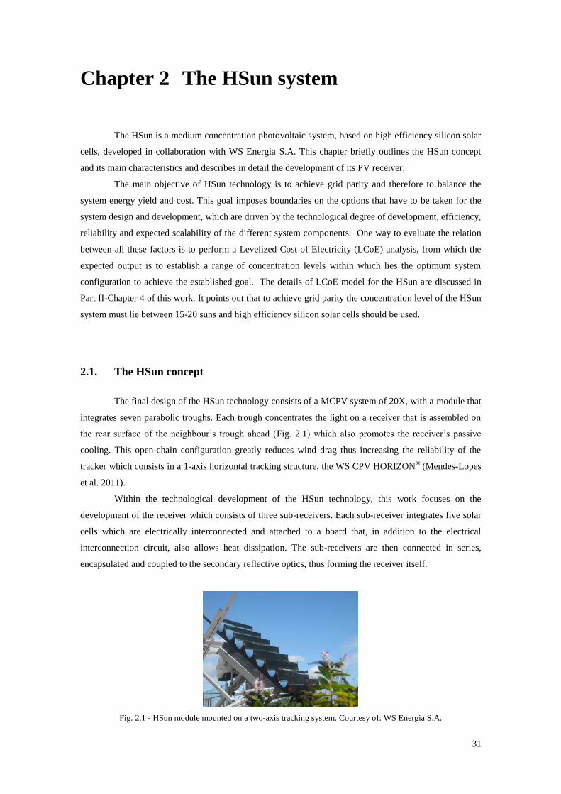
31

Chapter 2 The HSun system

The HSun is a medium concentration photovoltaic system, based on high efficiency silicon solar

cells, developed in collaboration with WS Energia S.A. This chapter briefly outlines the HSun concept

and its main characteristics and describes in detail the development of its PV receiver.

The main objective of HSun technology is to achieve grid parity and therefore to balance the

system energy yield and cost. This goal imposes boundaries on the options that have to be taken for the

system design and development, which are driven by the technological degree of development, efficiency,

reliability and expected scalability of the different system components. One way to evaluate the relation

between all these factors is to perform a Levelized Cost of Electricity (LCoE) analysis, from which the

expected output is to establish a range of concentration levels within which lies the optimum system

configuration to achieve the established goal. The details of LCoE model for the HSun are discussed in

Part II-Chapter 4 of this work. It points out that to achieve grid parity the concentration level of the HSun

system must lie between 15-20 suns and high efficiency silicon solar cells should be used.

2.1. The HSun concept

The final design of the HSun technology consists of a MCPV system of 20X, with a module that

integrates seven parabolic troughs. Each trough concentrates the light on a receiver that is assembled on

the rear surface of the neighbour’s trough ahead (Fig. 2.1) which also promotes the receiver’s passive

cooling. This open-chain configuration greatly reduces wind drag thus increasing the reliability of the

tracker which consists in a 1-axis horizontal tracking structure, the WS CPV HORIZON®

(Mendes-Lopes

et al. 2011).

Within the technological development of the HSun technology, this work focuses on the

development of the receiver which consists of three sub-receivers. Each sub-receiver integrates five solar

cells which are electrically interconnected and attached to a board that, in addition to the electrical

interconnection circuit, also allows heat dissipation. The sub-receivers are then connected in series,

encapsulated and coupled to the secondary reflective optics, thus forming the receiver itself.

Fig. 2.1 - HSun module mounted on a two-axis tracking system. Courtesy of: WS Energia S.A.

32

2.2. Solar cells for HSun system

Following the discussion of solar cells suitable to integrate CPV systems in Chapter 1, Section

1.3.3, HSun technology integrates high efficiency silicon solar cells. This section starts with a brief

review of the physics behind these devices and the most important parameters for the analysis of their

performance. Then, the main requirements for silicon solar cells operation under concentration are

described and, at the end, a comparison between alternative high efficiency silicon solar cells options is

performed.

2.2.1. Physics of silicon solar cells

Solar cells, the fundamental unit of a PV system, are typically made of semiconductor materials,

being crystalline silicon the material that holds the highest solar cells market share (Markvart 2000).

In a crystalline solar cell, the silicon atoms form a stable crystal. Each atom has four valence

electrons which are shared with four neighbouring atoms in order to reach a stable configuration. When

sunlight hits this structure, only photons with sufficient energy, i.e. higher than the semiconductor

bandgap, will transfer the energy to the shared electrons which achieve a higher energy state, being able

to participate in the conduction band, i.e. free to move and leaving a hole behind. This leads to an

additional conduction process consisting in a continual movement of the neighbouring electrons filling

the neighbouring hole. Hence, the excitation of a carrier from the valence band to the conducting band

creates carriers in both bands, i.e. electrons in the former and holes in the latter band. The concentration

of these carriers is called intrinsic carrier concentration and depends on the material temperature. With

increasing temperature, the electrons are likely to pass to the conduction band, which increases the

intrinsic carrier concentration, a feature that is very relevant to the solar cell efficiency. However, in order

to create electricity, the solar cell must have an electrical imbalance which forces the electrons to flow in

one direction. Such shift in the carriers balance is achieved by implantation of impurities (dopants) in the

silicon crystal lattice with other atoms. Two different layers are created: i) a n-type silicon layer which

has excess of electrons and a ii) p-type silicon layer with deficit of electrons, and consequently excess of

holes. The n-type layer is typically doped with Phosphorous, a V group element that has five electrons on

the valence band from which four electrons may form covalent bonds with the four silicon valence

electrons while the remaining electron is free to participate in the conduction band. On the other hand, the

p-type layer is typically doped with Boron, a III group element, that has only three valence electrons

which means that when interacting with silicon an electron will be missing thus standing one extra hole.

When these two layers are brought together in a solar cell, the excess of electrons on the n-type silicon

layer diffuse to the p-type layer while the holes perform the opposite path. This carrier diffusion leaves

behind exposed charges in the dopant atoms that are fixed in the crystal lattice which means that the n-

type layer becomes positively charged (positive ion cores) while the p-type layer is negatively charged

(negative ion cores). This way an electric field is created being the transition region between n-type and

p-type layers called depletion region which limits the diffusion of holes and electrons, keeping the holes

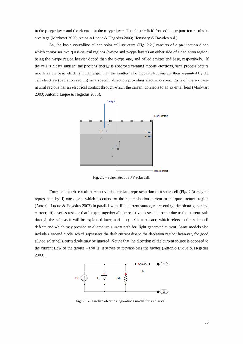
33

in the p-type layer and the electron in the n-type layer. The electric field formed in the junction results in

a voltage (Markvart 2000; Antonio Luque & Hegedus 2003; Honsberg & Bowden n.d.).

So, the basic crystalline silicon solar cell structure (Fig. 2.2.) consists of a pn-junction diode

which comprises two quasi-neutral regions (n-type and p-type layers) on either side of a depletion region,

being the n-type region heavier doped than the p-type one, and called emitter and base, respectively. If

the cell is hit by sunlight the photons energy is absorbed creating mobile electrons, such process occurs

mostly in the base which is much larger than the emitter. The mobile electrons are then separated by the

cell structure (depletion region) in a specific direction providing electric current. Each of these quasi-

neutral regions has an electrical contact through which the current connects to an external load (Markvart

2000; Antonio Luque & Hegedus 2003).

Fig. 2.2 - Schematic of a PV solar cell.

From an electric circuit perspective the standard representation of a solar cell (Fig. 2.3) may be

represented by: i) one diode, which accounts for the recombination current in the quasi-neutral region

(Antonio Luque & Hegedus 2003) in parallel with ii) a current source, representing the photo-generated

current; iii) a series resistor that lumped together all the resistive losses that occur due to the current path

through the cell, as it will be explained later; and iv) a shunt resistor, which refers to the solar cell

defects and which may provide an alternative current path for light-generated current. Some models also

include a second diode, which represents the dark current due to the depletion region; however, for good

silicon solar cells, such diode may be ignored. Notice that the direction of the current source is opposed to

the current flow of the diodes – that is, it serves to forward-bias the diodes (Antonio Luque & Hegedus

2003).

Fig. 2.3 - Standard electric single-diode model for a solar cell.

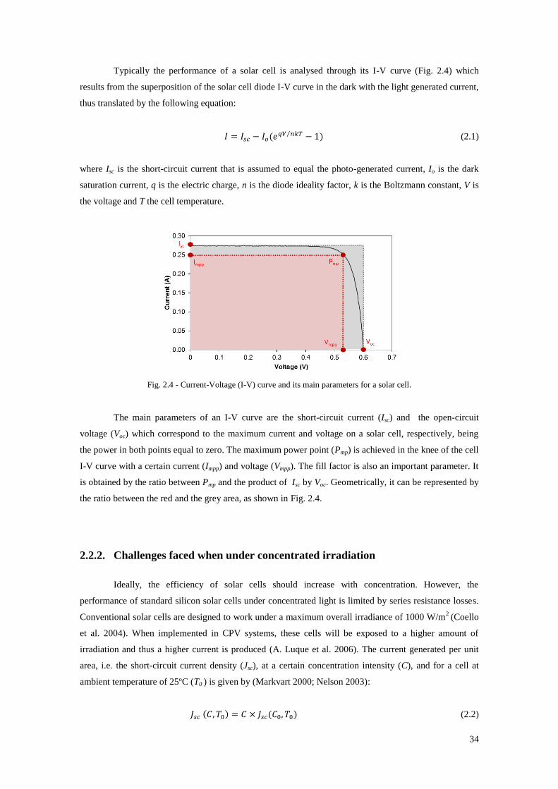
34

Typically the performance of a solar cell is analysed through its I-V curve (Fig. 2.4) which

results from the superposition of the solar cell diode I-V curve in the dark with the light generated current,

thus translated by the following equation:

⁄ (2.1)

where Isc is the short-circuit current that is assumed to equal the photo-generated current, Io is the dark

saturation current, q is the electric charge, n is the diode ideality factor, k is the Boltzmann constant, V is

the voltage and T the cell temperature.

Fig. 2.4 - Current-Voltage (I-V) curve and its main parameters for a solar cell.

The main parameters of an I-V curve are the short-circuit current (Isc) and the open-circuit

voltage (Voc) which correspond to the maximum current and voltage on a solar cell, respectively, being

the power in both points equal to zero. The maximum power point (Pmp) is achieved in the knee of the cell

I-V curve with a certain current (Impp) and voltage (Vmpp). The fill factor is also an important parameter. It

is obtained by the ratio between Pmp and the product of Isc by Voc. Geometrically, it can be represented by

the ratio between the red and the grey area, as shown in Fig. 2.4.

2.2.2. Challenges faced when under concentrated irradiation

Ideally, the efficiency of solar cells should increase with concentration. However, the

performance of standard silicon solar cells under concentrated light is limited by series resistance losses.

Conventional solar cells are designed to work under a maximum overall irradiance of 1000 W/m2

(Coello

et al. 2004). When implemented in CPV systems, these cells will be exposed to a higher amount of

irradiation and thus a higher current is produced (A. Luque et al. 2006). The current generated per unit

area, i.e. the short-circuit current density (Jsc), at a certain concentration intensity (C), and for a cell at

ambient temperature of 25ºC (T0 ) is given by (Markvart 2000; Nelson 2003):

(2.2)

35

where, Jsc(C0, T0) is the short-circuit current density at Standard Test Conditions (STC) with C0 equal to 1

sun, i.e. 1000W/m2.

The open-circuit voltage (Voc) also increases with concentration but with the logarithm of

concentration intensity (Markvart 2000; Nelson 2003):

(

)

(2.3)

where J0 is the saturation current density, and is the open-circuit voltage under STC.

If the cell fill factor (FF) remained constant then the power delivered by the cell should increase

by a factor

(

) (2.4)

and the efficiency by a factor:

(

) (2.5)

However, for a solar cell with a series resistance, Rs, the power dissipated through heat (Ploss),

i.e. the Joule resistance loss, is given by:

(2.6)

The current I flowing from the cell is proportional to the concentration, C. Based on eq. (2.2),

the power loss is given by:

(2.7)

Thus, when considering the series resistance, the FF will change instead of remaining a constant

value. We may estimate the FF by the following approximation (Honsberg & Bowden n.d.):

(2.8)

(

) (2.9)

(

) (2.10)

(

) (2.11)

where RCH is the characteristic resistance of the cell. If we define a normalized series resistance:

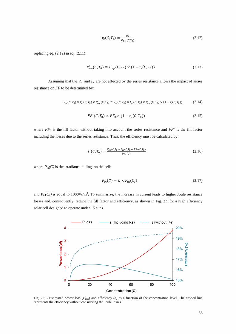
36

(2.12)

replacing eq. (2.12) in eq. (2.11):

(2.13)

Assuming that the Voc and Isc are not affected by the series resistance allows the impact of series

resistance on FF to be determined by:

(2.14)

(2.15)

where FF0 is the fill factor without taking into account the series resistance and FF’ is the fill factor

including the losses due to the series resistance. Thus, the efficiency must be calculated by:

(2.16)

where Pin(C) is the irradiance falling on the cell:

(2.17)

and Pin(C0) is equal to 1000W/m2. To summarize, the increase in current leads to higher Joule resistance

losses and, consequently, reduce the fill factor and efficiency, as shown in Fig. 2.5 for a high efficiency

solar cell designed to operate under 15 suns.

Fig. 2.5 - Estimated power loss (Ploss) and efficiency () as a function of the concentration level. The dashed line

represents the efficiency without considering the Joule losses.

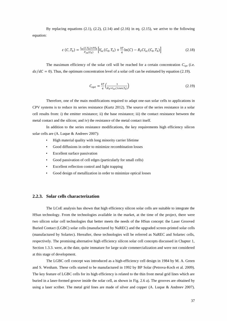
37

By replacing equations (2.1), (2.2), (2.14) and (2.16) in eq. (2.15), we arrive to the following

equation:

[

] (2.18)

The maximum efficiency of the solar cell will be reached for a certain concentration Copt (i.e.

⁄ ). Thus, the optimum concentration level of a solar cell can be estimated by equation (2.19).

(

) (2.19)

Therefore, one of the main modifications required to adapt one-sun solar cells to applications in

CPV systems is to reduce its series resistance (Kurtz 2012). The source of the series resistance in a solar

cell results from: i) the emitter resistance; ii) the base resistance; iii) the contact resistance between the

metal contact and the silicon; and iv) the resistance of the metal contact itself.

In addition to the series resistance modifications, the key requirements high efficiency silicon

solar cells are (A. Luque & Andreev 2007):

• High material quality with long minority carrier lifetime

• Good diffusions in order to minimize recombination losses

• Excellent surface passivation

• Good passivation of cell edges (particularly for small cells)

• Excellent reflection control and light trapping

• Good design of metallization in order to minimize optical losses

2.2.3. Solar cells characterization

The LCoE analysis has shown that high efficiency silicon solar cells are suitable to integrate the

HSun technology. From the technologies available in the market, at the time of the project, there were

two silicon solar cell technologies that better meets the needs of the HSun concept: the Laser Grooved

Buried Contact (LGBC) solar cells (manufactured by NaREC) and the upgraded screen-printed solar cells

(manufactured by Solartec). Hereafter, these technologies will be referred as NaREC and Solartec cells,

respectively. The promising alternative high efficiency silicon solar cell concepts discussed in Chapter 1,

Section 1.3.3. were, at the date, quite immature for large scale commercialization and were not considered

at this stage of development.

The LGBC cell concept was introduced as a high-efficiency cell design in 1984 by M. A. Green

and S. Wenham. These cells started to be manufactured in 1992 by BP Solar (Petrova-Koch et al. 2009).

The key feature of LGBC cells for its high efficiency is related to the thin front metal grid lines which are

buried in a laser-formed groove inside the solar cell, as shown in Fig. 2.6 a). The grooves are obtained by

using a laser scriber. The metal grid lines are made of silver and copper (A. Luque & Andreev 2007).

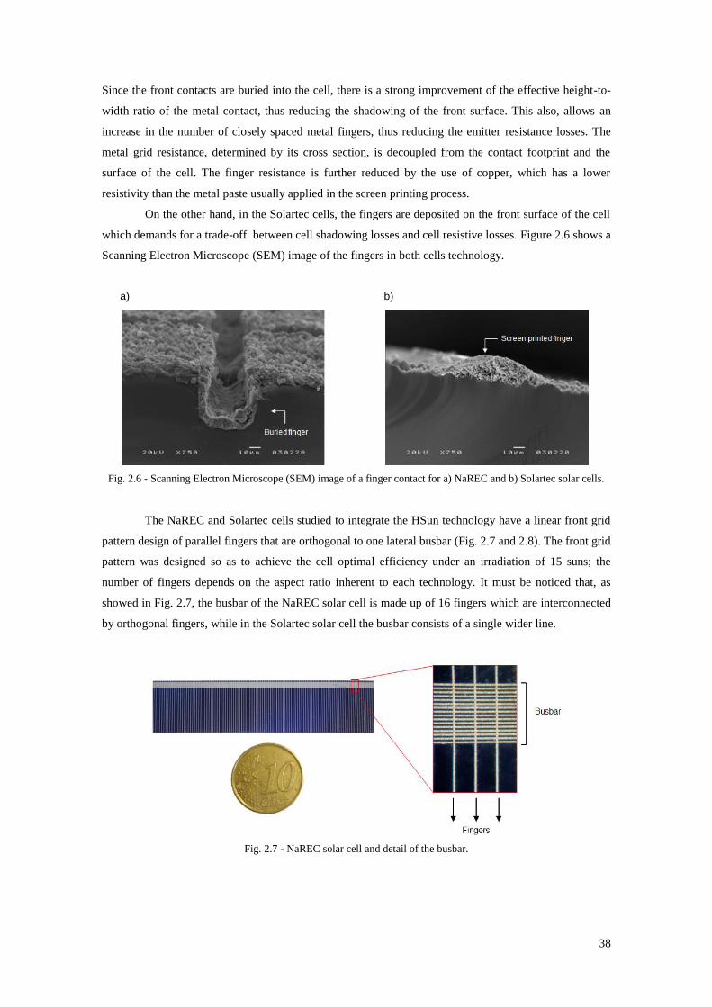
38

Since the front contacts are buried into the cell, there is a strong improvement of the effective height-to-

width ratio of the metal contact, thus reducing the shadowing of the front surface. This also, allows an

increase in the number of closely spaced metal fingers, thus reducing the emitter resistance losses. The

metal grid resistance, determined by its cross section, is decoupled from the contact footprint and the

surface of the cell. The finger resistance is further reduced by the use of copper, which has a lower

resistivity than the metal paste usually applied in the screen printing process.

On the other hand, in the Solartec cells, the fingers are deposited on the front surface of the cell

which demands for a trade-off between cell shadowing losses and cell resistive losses. Figure 2.6 shows a

Scanning Electron Microscope (SEM) image of the fingers in both cells technology.

a) b)

Fig. 2.6 - Scanning Electron Microscope (SEM) image of a finger contact for a) NaREC and b) Solartec solar cells.

The NaREC and Solartec cells studied to integrate the HSun technology have a linear front grid

pattern design of parallel fingers that are orthogonal to one lateral busbar (Fig. 2.7 and 2.8). The front grid

pattern was designed so as to achieve the cell optimal efficiency under an irradiation of 15 suns; the

number of fingers depends on the aspect ratio inherent to each technology. It must be noticed that, as

showed in Fig. 2.7, the busbar of the NaREC solar cell is made up of 16 fingers which are interconnected

by orthogonal fingers, while in the Solartec solar cell the busbar consists of a single wider line.

Fig. 2.7 - NaREC solar cell and detail of the busbar.

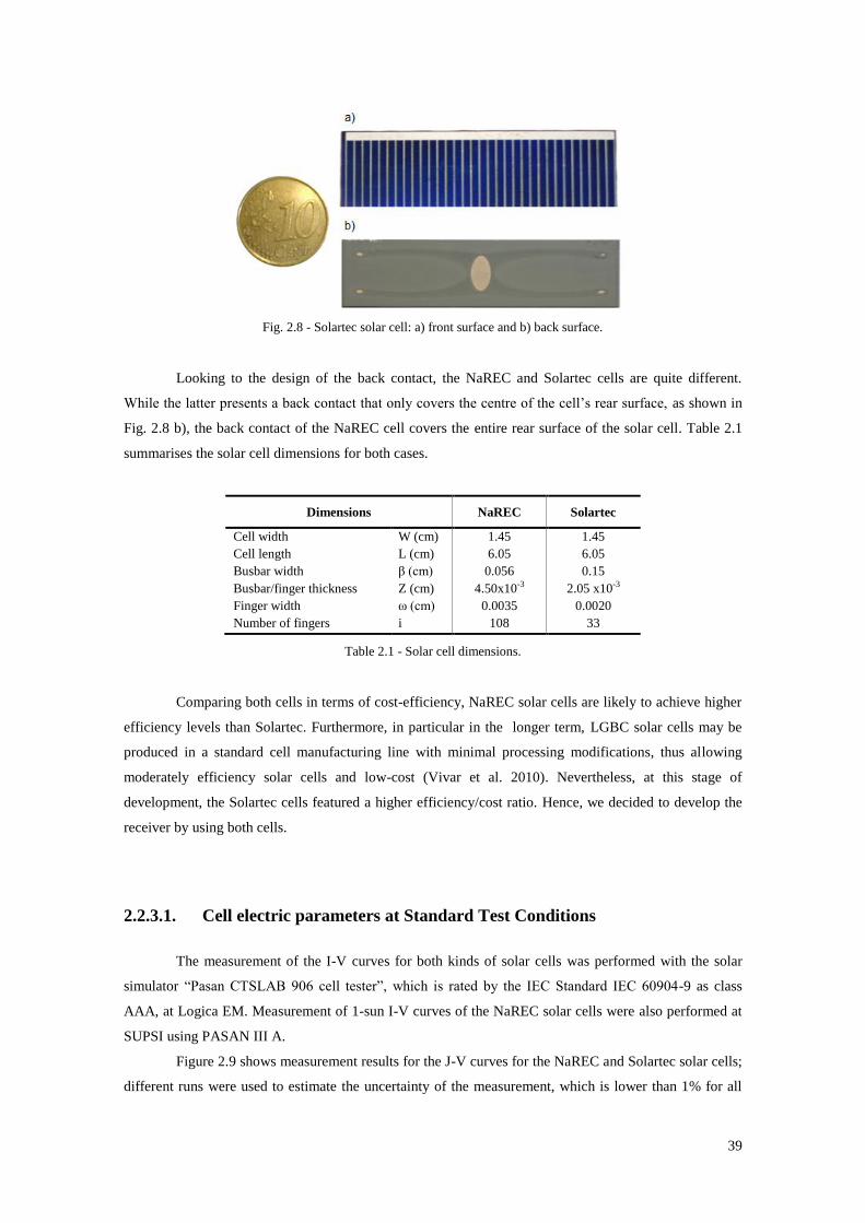
39

Fig. 2.8 - Solartec solar cell: a) front surface and b) back surface.

Looking to the design of the back contact, the NaREC and Solartec cells are quite different.

While the latter presents a back contact that only covers the centre of the cell’s rear surface, as shown in

Fig. 2.8 b), the back contact of the NaREC cell covers the entire rear surface of the solar cell. Table 2.1

summarises the solar cell dimensions for both cases.

Dimensions NaREC Solartec

Cell width W (cm) 1.45 1.45

Cell length L (cm) 6.05 6.05

Busbar width β (cm) 0.056 0.15

Busbar/finger thickness Z (cm) 4.50x10-3 2.05 x10-3

Finger width ω (cm) 0.0035 0.0020

Number of fingers i 108 33

Table 2.1 - Solar cell dimensions.

Comparing both cells in terms of cost-efficiency, NaREC solar cells are likely to achieve higher

efficiency levels than Solartec. Furthermore, in particular in the longer term, LGBC solar cells may be

produced in a standard cell manufacturing line with minimal processing modifications, thus allowing

moderately efficiency solar cells and low-cost (Vivar et al. 2010). Nevertheless, at this stage of

development, the Solartec cells featured a higher efficiency/cost ratio. Hence, we decided to develop the

receiver by using both cells.

2.2.3.1. Cell electric parameters at Standard Test Conditions

The measurement of the I-V curves for both kinds of solar cells was performed with the solar

simulator “Pasan CTSLAB 906 cell tester”, which is rated by the IEC Standard IEC 60904-9 as class

AAA, at Logica EM. Measurement of 1-sun I-V curves of the NaREC solar cells were also performed at

SUPSI using PASAN III A.

Figure 2.9 shows measurement results for the J-V curves for the NaREC and Solartec solar cells;

different runs were used to estimate the uncertainty of the measurement, which is lower than 1% for all

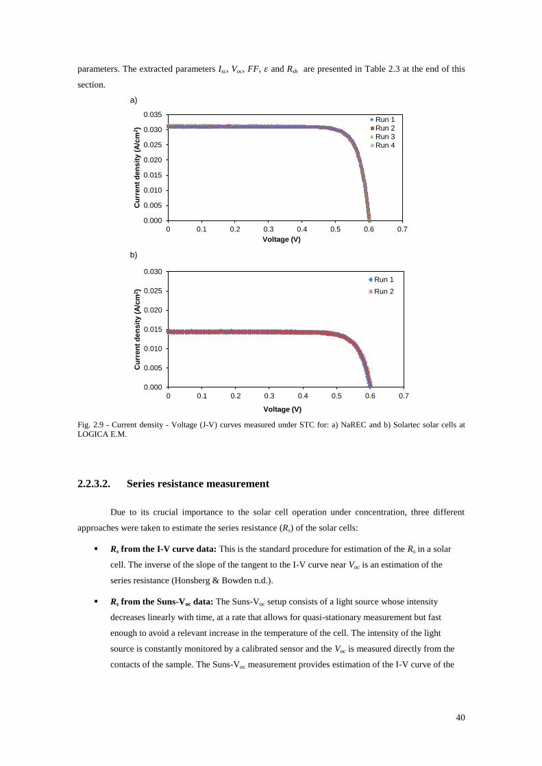
40

parameters. The extracted parameters Isc, Voc, FF, and Rsh are presented in Table 2.3 at the end of this

section.

a)

b)

Fig. 2.9 - Current density - Voltage (J-V) curves measured under STC for: a) NaREC and b) Solartec solar cells at

LOGICA E.M.

2.2.3.2. Series resistance measurement

Due to its crucial importance to the solar cell operation under concentration, three different

approaches were taken to estimate the series resistance (Rs) of the solar cells:

Rs from the I-V curve data: This is the standard procedure for estimation of the Rs in a solar

cell. The inverse of the slope of the tangent to the I-V curve near Voc is an estimation of the

series resistance (Honsberg & Bowden n.d.).

Rs from the Suns-Voc data: The Suns-Voc setup consists of a light source whose intensity

decreases linearly with time, at a rate that allows for quasi-stationary measurement but fast

enough to avoid a relevant increase in the temperature of the cell. The intensity of the light

source is constantly monitored by a calibrated sensor and the Voc is measured directly from the

contacts of the sample. The Suns-Voc measurement provides estimation of the I-V curve of the

0.000

0.005

0.010

0.015

0.020

0.025

0.030

0.035

0 0.1 0.2 0.3 0.4 0.5 0.6 0.7

Cu

rren

t d

en

sit

y (

A/c

m2)

Voltage (V)

Run 1Run 2Run 3Run 4

0.000

0.005

0.010

0.015

0.020

0.025

0.030

0 0.1 0.2 0.3 0.4 0.5 0.6 0.7

Cu

rren

t d

en

sit

y (

A/c

m2)

Voltage (V)

Run 1

Run 2

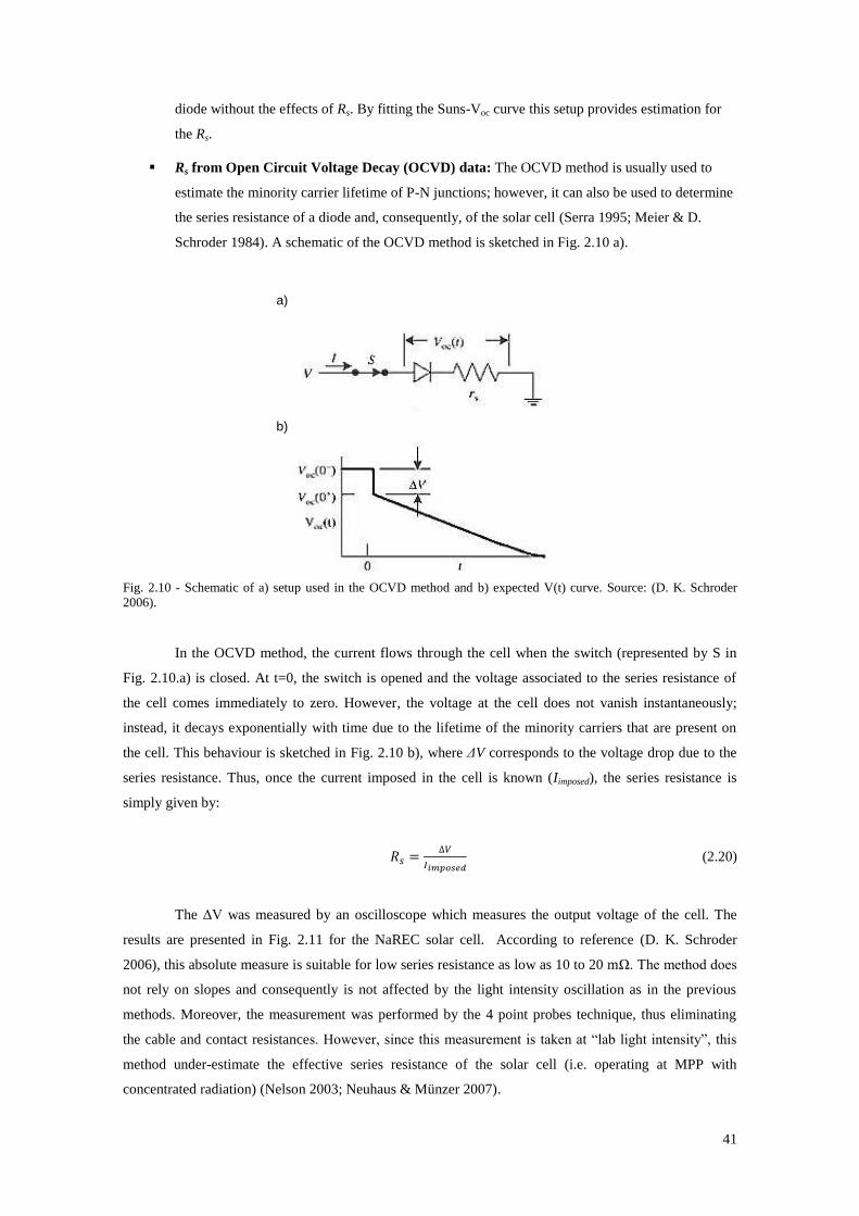
41

diode without the effects of Rs. By fitting the Suns-Voc curve this setup provides estimation for

the Rs.

Rs from Open Circuit Voltage Decay (OCVD) data: The OCVD method is usually used to

estimate the minority carrier lifetime of P-N junctions; however, it can also be used to determine

the series resistance of a diode and, consequently, of the solar cell (Serra 1995; Meier & D.

Schroder 1984). A schematic of the OCVD method is sketched in Fig. 2.10 a).

a)

b)

Fig. 2.10 - Schematic of a) setup used in the OCVD method and b) expected V(t) curve. Source: (D. K. Schroder

2006).

In the OCVD method, the current flows through the cell when the switch (represented by S in

Fig. 2.10.a) is closed. At t=0, the switch is opened and the voltage associated to the series resistance of

the cell comes immediately to zero. However, the voltage at the cell does not vanish instantaneously;

instead, it decays exponentially with time due to the lifetime of the minority carriers that are present on

the cell. This behaviour is sketched in Fig. 2.10 b), where ΔV corresponds to the voltage drop due to the

series resistance. Thus, once the current imposed in the cell is known (Iimposed), the series resistance is

simply given by:

(2.20)

The ΔV was measured by an oscilloscope which measures the output voltage of the cell. The

results are presented in Fig. 2.11 for the NaREC solar cell. According to reference (D. K. Schroder

2006), this absolute measure is suitable for low series resistance as low as 10 to 20 mΩ. The method does

not rely on slopes and consequently is not affected by the light intensity oscillation as in the previous

methods. Moreover, the measurement was performed by the 4 point probes technique, thus eliminating

the cable and contact resistances. However, since this measurement is taken at “lab light intensity”, this

method under-estimate the effective series resistance of the solar cell (i.e. operating at MPP with

concentrated radiation) (Nelson 2003; Neuhaus & Münzer 2007).

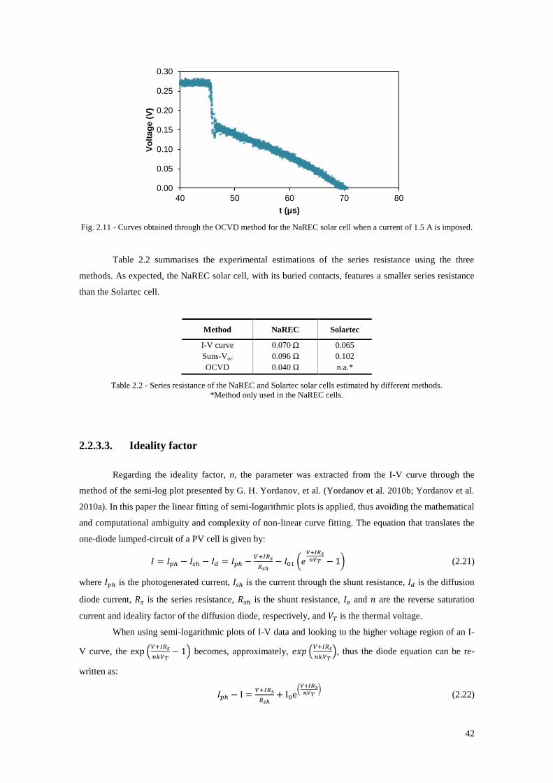
42

Fig. 2.11 - Curves obtained through the OCVD method for the NaREC solar cell when a current of 1.5 A is imposed.

Table 2.2 summarises the experimental estimations of the series resistance using the three

methods. As expected, the NaREC solar cell, with its buried contacts, features a smaller series resistance

than the Solartec cell.

Method NaREC Solartec

I-V curve 0.070 Ω 0.065

Suns-Voc 0.096 Ω 0.102

OCVD 0.040 Ω n.a.*

Table 2.2 - Series resistance of the NaREC and Solartec solar cells estimated by different methods.

*Method only used in the NaREC cells.

2.2.3.3. Ideality factor

Regarding the ideality factor, n, the parameter was extracted from the I-V curve through the

method of the semi-log plot presented by G. H. Yordanov, et al. (Yordanov et al. 2010b; Yordanov et al.

2010a). In this paper the linear fitting of semi-logarithmic plots is applied, thus avoiding the mathematical

and computational ambiguity and complexity of non-linear curve fitting. The equation that translates the

one-diode lumped-circuit of a PV cell is given by:

(

) (2.21)

where is the photogenerated current, is the current through the shunt resistance, is the diffusion

diode current, is the series resistance, is the shunt resistance, and are the reverse saturation

current and ideality factor of the diffusion diode, respectively, and is the thermal voltage.

When using semi-logarithmic plots of I-V data and looking to the higher voltage region of an I-

V curve, the (

) becomes, approximately, (

), thus the diode equation can be re-

written as:

(

) (2.22)

0.00

0.05

0.10

0.15

0.20

0.25

0.30

40 50 60 70 80

Vo

lta

ge

(V

)

t (μs)

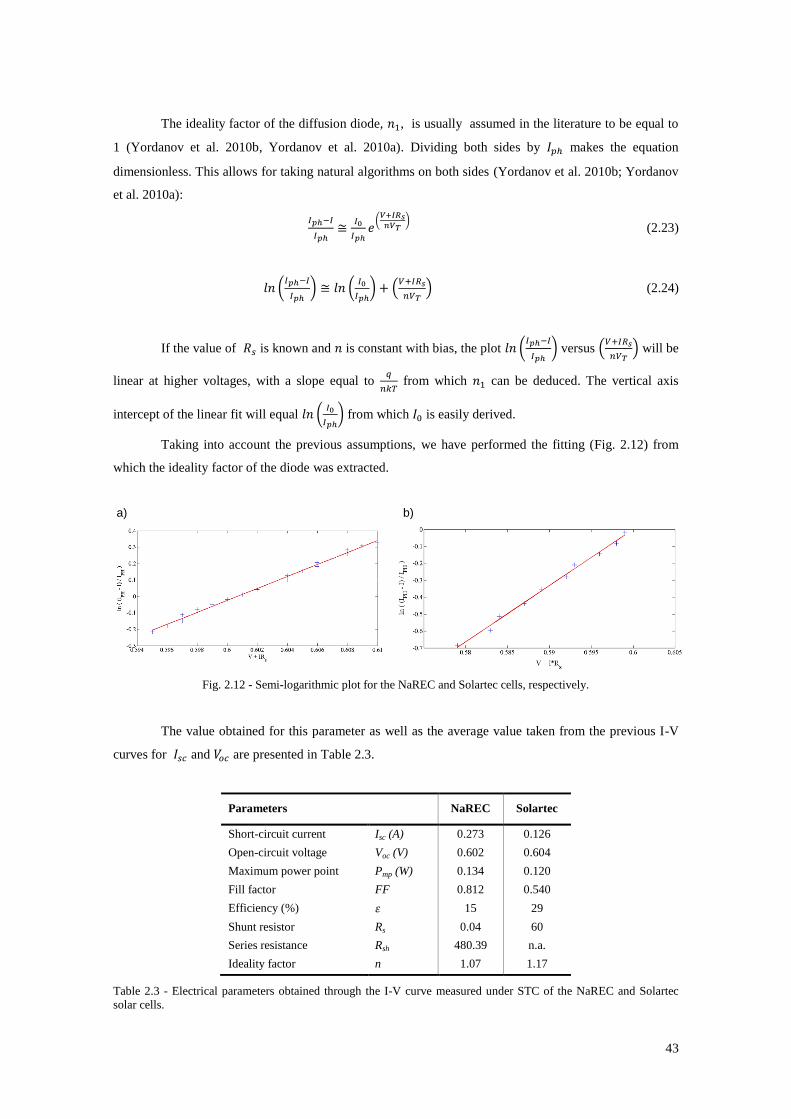
43

The ideality factor of the diffusion diode, , is usually assumed in the literature to be equal to

1 (Yordanov et al. 2010b, Yordanov et al. 2010a). Dividing both sides by makes the equation

dimensionless. This allows for taking natural algorithms on both sides (Yordanov et al. 2010b; Yordanov

et al. 2010a):

(

) (2.23)

(

) (

) (

) (2.24)

If the value of is known and is constant with bias, the plot (

) versus (

) will be

linear at higher voltages, with a slope equal to

from which can be deduced. The vertical axis

intercept of the linear fit will equal (

) from which is easily derived.

Taking into account the previous assumptions, we have performed the fitting (Fig. 2.12) from

which the ideality factor of the diode was extracted.

a) b)

Fig. 2.12 - Semi-logarithmic plot for the NaREC and Solartec cells, respectively.

The value obtained for this parameter as well as the average value taken from the previous I-V

curves for and are presented in Table 2.3.

Parameters NaREC Solartec

Short-circuit current Isc (A) 0.273 0.126

Open-circuit voltage Voc (V) 0.602 0.604

Maximum power point Pmp (W) 0.134 0.120

Fill factor FF 0.812 0.540

Efficiency (%) 15 29

Shunt resistor Rs 0.04 60

Series resistance Rsh 480.39 n.a.

Ideality factor n 1.07 1.17

Table 2.3 - Electrical parameters obtained through the I-V curve measured under STC of the NaREC and Solartec

solar cells.

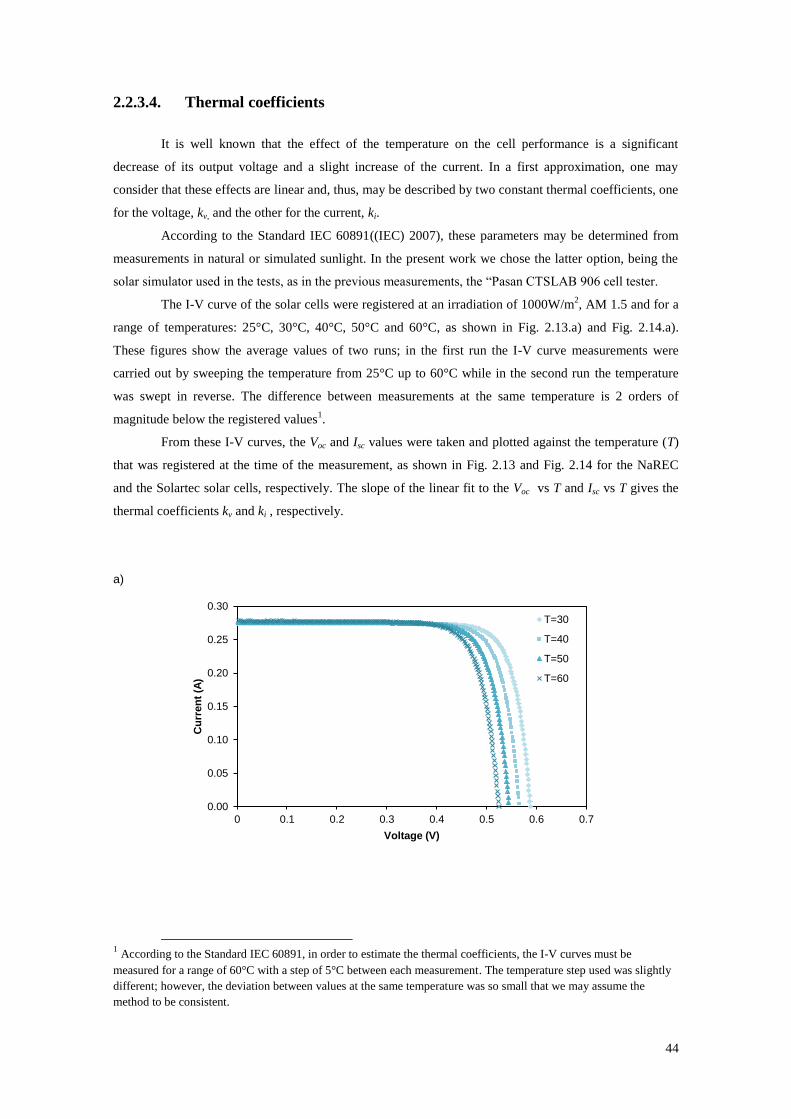
44

2.2.3.4. Thermal coefficients

It is well known that the effect of the temperature on the cell performance is a significant

decrease of its output voltage and a slight increase of the current. In a first approximation, one may

consider that these effects are linear and, thus, may be described by two constant thermal coefficients, one

for the voltage, kv, and the other for the current, ki.

According to the Standard IEC 60891((IEC) 2007), these parameters may be determined from

measurements in natural or simulated sunlight. In the present work we chose the latter option, being the

solar simulator used in the tests, as in the previous measurements, the “Pasan CTSLAB 906 cell tester.

The I-V curve of the solar cells were registered at an irradiation of 1000W/m2, AM 1.5 and for a

range of temperatures: 25°C, 30°C, 40°C, 50°C and 60°C, as shown in Fig. 2.13.a) and Fig. 2.14.a).

These figures show the average values of two runs; in the first run the I-V curve measurements were

carried out by sweeping the temperature from 25°C up to 60°C while in the second run the temperature

was swept in reverse. The difference between measurements at the same temperature is 2 orders of

magnitude below the registered values1.

From these I-V curves, the Voc and Isc values were taken and plotted against the temperature (T)

that was registered at the time of the measurement, as shown in Fig. 2.13 and Fig. 2.14 for the NaREC

and the Solartec solar cells, respectively. The slope of the linear fit to the Voc vs T and Isc vs T gives the

thermal coefficients kv and ki , respectively.

a)

1 According to the Standard IEC 60891, in order to estimate the thermal coefficients, the I-V curves must be

measured for a range of 60°C with a step of 5°C between each measurement. The temperature step used was slightly

different; however, the deviation between values at the same temperature was so small that we may assume the

method to be consistent.

0.00

0.05

0.10

0.15

0.20

0.25

0.30

0 0.1 0.2 0.3 0.4 0.5 0.6 0.7

Cu

rren

t (A

)

Voltage (V)

T=30

T=40

T=50

T=60

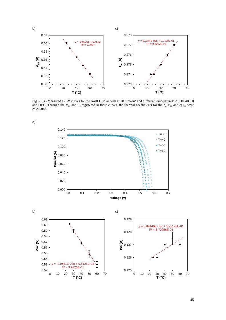
45

b) c)

Fig. 2.13 - Measured a) I-V curves for the NaREC solar cells at 1000 W/m2 and different temperatures: 25, 30, 40, 50

and 60°C. Through the Voc and Isc registered in these curves, the thermal coefficients for the b) Voc and c) Isc were

calculated.

a)

b)

c)

y = -0.0021x + 0.6532 R² = 0.9987

0.50

0.52

0.54

0.56

0.58

0.60

0.62

0 20 40 60 80

Vo

c (

V)

T (°C)

y = 9.0244E-05x + 2.7150E-01 R² = 9.8207E-01

0.273

0.274

0.275

0.276

0.277

0.278

0 20 40 60 80

I sc (

A)

T (°C)

0.000

0.020

0.040

0.060

0.080

0.100

0.120

0.140

0.0 0.1 0.2 0.3 0.4 0.5 0.6 0.7

Cu

rren

t (A

)

Voltage (V)

T=30

T=40

T=50

T=60

y = -2.0451E-03x + 6.5125E-01 R² = 9.9723E-01

0.52

0.53

0.54

0.55

0.56

0.57

0.58

0.59

0.60

0.61

0 10 20 30 40 50 60 70

Vo

c (

V)

T (°C)

y = 3.84146E-05x + 1.25125E-01 R² = 6.72256E-01

0.125

0.126

0.127

0.128

0.129

0 10 20 30 40 50 60 70

Isc

(A

)

T (°C)

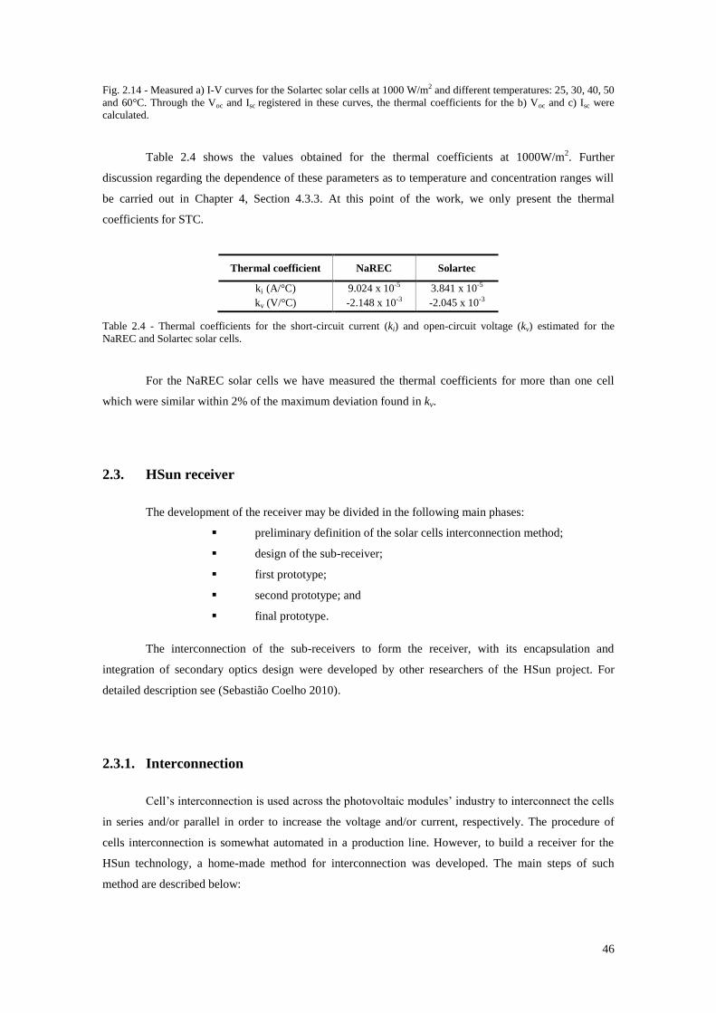
46

Fig. 2.14 - Measured a) I-V curves for the Solartec solar cells at 1000 W/m2 and different temperatures: 25, 30, 40, 50

and 60°C. Through the Voc and Isc registered in these curves, the thermal coefficients for the b) Voc and c) Isc were

calculated.

Table 2.4 shows the values obtained for the thermal coefficients at 1000W/m2. Further

discussion regarding the dependence of these parameters as to temperature and concentration ranges will

be carried out in Chapter 4, Section 4.3.3. At this point of the work, we only present the thermal

coefficients for STC.

Thermal coefficient NaREC Solartec

ki (A/°C) 9.024 x 10-5 3.841 x 10-5

kv (V/°C) -2.148 x 10-3 -2.045 x 10-3

Table 2.4 - Thermal coefficients for the short-circuit current (ki) and open-circuit voltage (kv) estimated for the

NaREC and Solartec solar cells.

For the NaREC solar cells we have measured the thermal coefficients for more than one cell

which were similar within 2% of the maximum deviation found in kv.

2.3. HSun receiver

The development of the receiver may be divided in the following main phases:

preliminary definition of the solar cells interconnection method;

design of the sub-receiver;

first prototype;

second prototype; and

final prototype.

The interconnection of the sub-receivers to form the receiver, with its encapsulation and

integration of secondary optics design were developed by other researchers of the HSun project. For

detailed description see (Sebastião Coelho 2010).

2.3.1. Interconnection

Cell’s interconnection is used across the photovoltaic modules’ industry to interconnect the cells

in series and/or parallel in order to increase the voltage and/or current, respectively. The procedure of

cells interconnection is somewhat automated in a production line. However, to build a receiver for the

HSun technology, a home-made method for interconnection was developed. The main steps of such

method are described below:

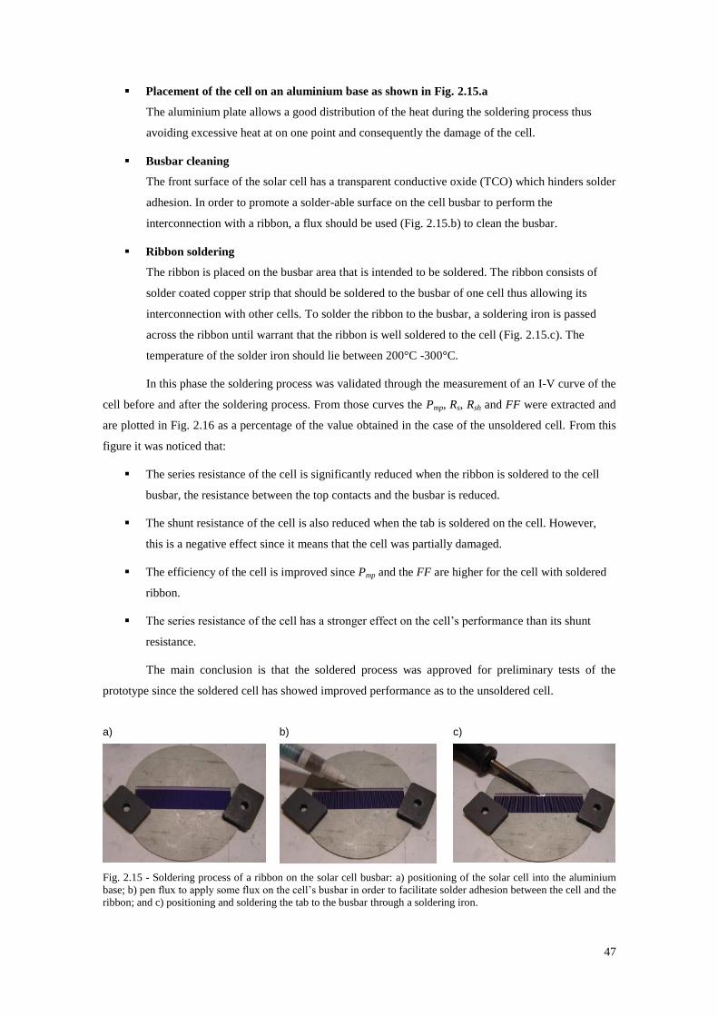
47

Placement of the cell on an aluminium base as shown in Fig. 2.15.a

The aluminium plate allows a good distribution of the heat during the soldering process thus

avoiding excessive heat at on one point and consequently the damage of the cell.

Busbar cleaning

The front surface of the solar cell has a transparent conductive oxide (TCO) which hinders solder

adhesion. In order to promote a solder-able surface on the cell busbar to perform the

interconnection with a ribbon, a flux should be used (Fig. 2.15.b) to clean the busbar.

Ribbon soldering

The ribbon is placed on the busbar area that is intended to be soldered. The ribbon consists of

solder coated copper strip that should be soldered to the busbar of one cell thus allowing its

interconnection with other cells. To solder the ribbon to the busbar, a soldering iron is passed

across the ribbon until warrant that the ribbon is well soldered to the cell (Fig. 2.15.c). The

temperature of the solder iron should lie between 200°C -300°C.

In this phase the soldering process was validated through the measurement of an I-V curve of the

cell before and after the soldering process. From those curves the Pmp, Rs, Rsh and FF were extracted and

are plotted in Fig. 2.16 as a percentage of the value obtained in the case of the unsoldered cell. From this

figure it was noticed that:

The series resistance of the cell is significantly reduced when the ribbon is soldered to the cell

busbar, the resistance between the top contacts and the busbar is reduced.

The shunt resistance of the cell is also reduced when the tab is soldered on the cell. However,

this is a negative effect since it means that the cell was partially damaged.

The efficiency of the cell is improved since Pmp and the FF are higher for the cell with soldered

ribbon.

The series resistance of the cell has a stronger effect on the cell’s performance than its shunt

resistance.

The main conclusion is that the soldered process was approved for preliminary tests of the

prototype since the soldered cell has showed improved performance as to the unsoldered cell.

a) b) c)

Fig. 2.15 - Soldering process of a ribbon on the solar cell busbar: a) positioning of the solar cell into the aluminium

base; b) pen flux to apply some flux on the cell’s busbar in order to facilitate solder adhesion between the cell and the

ribbon; and c) positioning and soldering the tab to the busbar through a soldering iron.

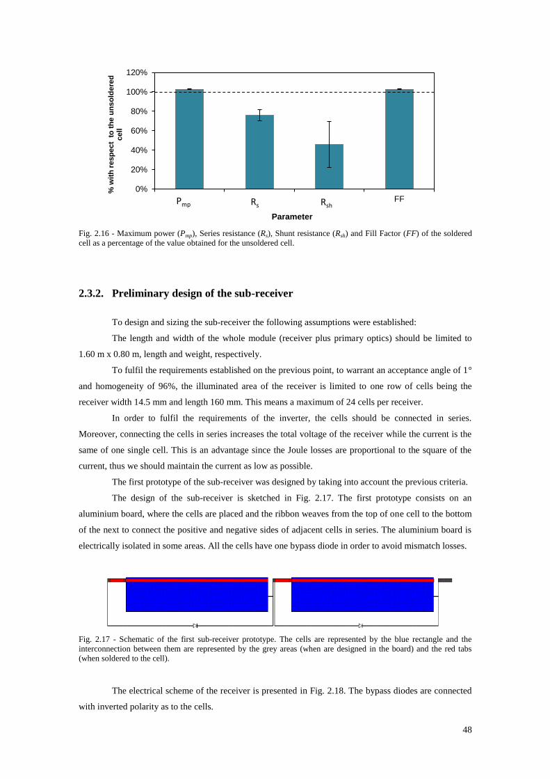
48

Fig. 2.16 - Maximum power (Pmp), Series resistance (Rs), Shunt resistance (Rsh) and Fill Factor (FF) of the soldered

cell as a percentage of the value obtained for the unsoldered cell.

2.3.2. Preliminary design of the sub-receiver

To design and sizing the sub-receiver the following assumptions were established:

The length and width of the whole module (receiver plus primary optics) should be limited to

1.60 m x 0.80 m, length and weight, respectively.

To fulfil the requirements established on the previous point, to warrant an acceptance angle of 1°

and homogeneity of 96%, the illuminated area of the receiver is limited to one row of cells being the

receiver width 14.5 mm and length 160 mm. This means a maximum of 24 cells per receiver.

In order to fulfil the requirements of the inverter, the cells should be connected in series.

Moreover, connecting the cells in series increases the total voltage of the receiver while the current is the

same of one single cell. This is an advantage since the Joule losses are proportional to the square of the

current, thus we should maintain the current as low as possible.

The first prototype of the sub-receiver was designed by taking into account the previous criteria.

The design of the sub-receiver is sketched in Fig. 2.17. The first prototype consists on an

aluminium board, where the cells are placed and the ribbon weaves from the top of one cell to the bottom

of the next to connect the positive and negative sides of adjacent cells in series. The aluminium board is

electrically isolated in some areas. All the cells have one bypass diode in order to avoid mismatch losses.

Fig. 2.17 - Schematic of the first sub-receiver prototype. The cells are represented by the blue rectangle and the

interconnection between them are represented by the grey areas (when are designed in the board) and the red tabs

(when soldered to the cell).

The electrical scheme of the receiver is presented in Fig. 2.18. The bypass diodes are connected

with inverted polarity as to the cells.

0%

20%

40%

60%

80%

100%

120%

Pmax Rs Rsh FF

% w

ith

resp

ect

to

th

e u

ns

old

ere

d

cell

Parameter

Pmp Rs Rsh

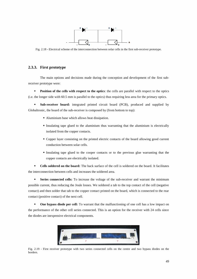
49

Fig. 2.18 - Electrical scheme of the interconnection between solar cells in the first sub-receiver prototype.

2.3.3. First prototype

The main options and decisions made during the conception and development of the first sub-

receiver prototype were:

Position of the cells with respect to the optics: the cells are parallel with respect to the optics

(i.e. the longer side with 60.5 mm is parallel to the optics) thus requiring less area for the primary optics.

Sub-receiver board: integrated printed circuit board (PCB), produced and supplied by

Globaltronic, the board of the sub-receiver is composed by (from bottom to top):

Aluminium base which allows heat dissipation.

Insulating tape glued to the aluminium thus warranting that the aluminium is electrically

isolated from the copper contacts.

Copper layer consisting on the printed electric contacts of the board allowing good current

conduction between solar cells.

Insulating tape glued to the cooper contacts or to the previous glue warranting that the

copper contacts are electrically isolated.

Cells soldered on the board: The back surface of the cell is soldered on the board. It facilitates

the interconnection between cells and increases the soldered area.

Series connected cells: To increase the voltage of the sub-receiver and warrant the minimum

possible current, thus reducing the Joule losses. We soldered a tab to the top contact of the cell (negative

contact) and then solder that tab to the copper contact printed on the board, which is connected to the rear

contact (positive contact) of the next cell.

One bypass diode per cell: To warrant that the malfunctioning of one cell has a low impact on

the performance of the other cell series connected. This is an option for the receiver with 24 cells since

the diodes are inexpensive electrical components.

Fig. 2.19 - First receiver prototype with two series connected cells on the centre and two bypass diodes on the

borders.

50

The following structural options were considered unsuitable to integrate the receiver:

Soldering of the entire solar cell back contact on the board: Entire cell soldering requires a

high quantity of flux and high quantity of soldering paste which can overflow and damage or short-circuit

the cell. Moreover, different materials present different coefficients of thermal expansion, which may

easily lead to cracks on the cell if the whole back surface is soldered to the board.

Soldering the tabs before soldering the cells on the board: We should solder the tab on the

cells only after the cell is soldered on the board, otherwise, when passing in the soldering furnace a

displacement of the ribbon may occur.

At this phase, the following aspects were pointed out as requiring further investigation to

optimize the receiver performance:

Resizing of the cells: The cells area may be changed to 14.5 mm x 30 mm. Such modification

increases the voltage and reduces the current of the module, which further reduces the Joule losses.

Resizing of the cells also facilitate industrial handling during the packaging process.

Aluminium board for the receiver: During the first prototype manufacturing, the heat applied

during the soldering process lead to the deformation of the aluminium board. Other manufacturing

temperature ranges should be tested.

2.3.4. Second prototype

The mounting process of the sub-receiver is briefly described by the following steps:

Placement of the thermal tape on the PCB (orange rectangles in Fig. 2.20). The

thermal tape promotes the heat dissipation between the unsoldered back contact of

the cell and the PCB. Moreover, the thermal tape helps to avoid displacement of

the cells from its position during the soldering process.

Placement of the soldering paste on:

The squares of PCB that are soldered to the back surface of the

solar cell (light blue circle in Fig. 2.20).

The top strip of each receiver, where the bussing ribbon will be

soldered.

Removal of the protective film of thermal tape and placement of the solar cells.

Placement of the diode on the PCB.

Placement of the bussing ribbon on the PCB (dark blue line in Fig. 2.20).

The sub-receiver is placed in a belt furnace for the soldering process.

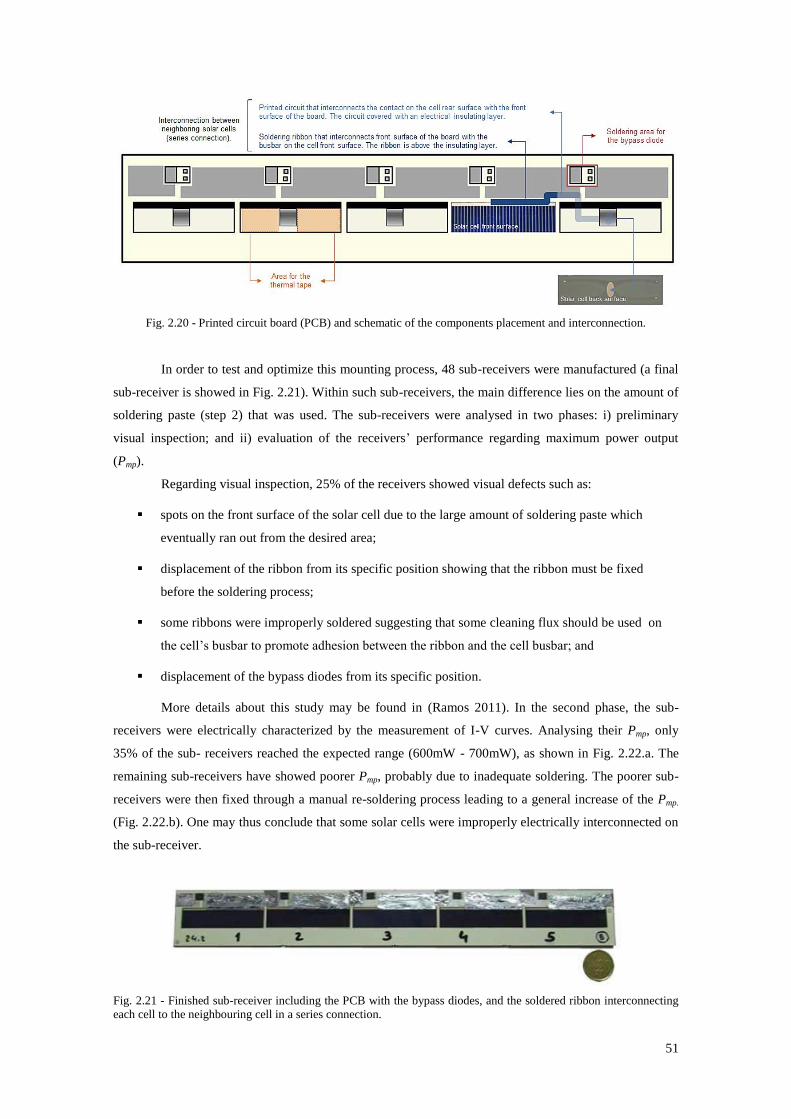
51

Fig. 2.20 - Printed circuit board (PCB) and schematic of the components placement and interconnection.

In order to test and optimize this mounting process, 48 sub-receivers were manufactured (a final

sub-receiver is showed in Fig. 2.21). Within such sub-receivers, the main difference lies on the amount of

soldering paste (step 2) that was used. The sub-receivers were analysed in two phases: i) preliminary

visual inspection; and ii) evaluation of the receivers’ performance regarding maximum power output

(Pmp).

Regarding visual inspection, 25% of the receivers showed visual defects such as:

spots on the front surface of the solar cell due to the large amount of soldering paste which

eventually ran out from the desired area;

displacement of the ribbon from its specific position showing that the ribbon must be fixed

before the soldering process;

some ribbons were improperly soldered suggesting that some cleaning flux should be used on

the cell’s busbar to promote adhesion between the ribbon and the cell busbar; and

displacement of the bypass diodes from its specific position.

More details about this study may be found in (Ramos 2011). In the second phase, the sub-

receivers were electrically characterized by the measurement of I-V curves. Analysing their Pmp, only

35% of the sub- receivers reached the expected range (600mW - 700mW), as shown in Fig. 2.22.a. The

remaining sub-receivers have showed poorer Pmp, probably due to inadequate soldering. The poorer sub-

receivers were then fixed through a manual re-soldering process leading to a general increase of the Pmp.

(Fig. 2.22.b). One may thus conclude that some solar cells were improperly electrically interconnected on

the sub-receiver.

Fig. 2.21 - Finished sub-receiver including the PCB with the bypass diodes, and the soldered ribbon interconnecting

each cell to the neighbouring cell in a series connection.

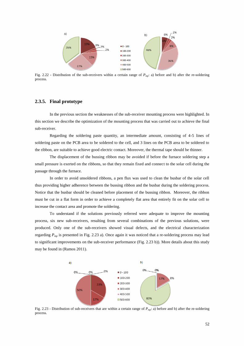
52

Fig. 2.22 - Distribution of the sub-receivers within a certain range of Pmp: a) before and b) after the re-soldering

process.

2.3.5. Final prototype

In the previous section the weaknesses of the sub-receiver mounting process were highlighted. In

this section we describe the optimization of the mounting process that was carried out to achieve the final

sub-receiver.

Regarding the soldering paste quantity, an intermediate amount, consisting of 4-5 lines of

soldering paste on the PCB area to be soldered to the cell, and 3 lines on the PCB area to be soldered to

the ribbon, are suitable to achieve good electric contact. Moreover, the thermal tape should be thinner.

The displacement of the bussing ribbon may be avoided if before the furnace soldering step a

small pressure is exerted on the ribbons, so that they remain fixed and connect to the solar cell during the

passage through the furnace.

In order to avoid unsoldered ribbons, a pen flux was used to clean the busbar of the solar cell

thus providing higher adherence between the bussing ribbon and the busbar during the soldering process.

Notice that the busbar should be cleaned before placement of the bussing ribbon. Moreover, the ribbon

must be cut in a flat form in order to achieve a completely flat area that entirely fit on the solar cell to

increase the contact area and promote the soldering.

To understand if the solutions previously referred were adequate to improve the mounting

process, six new sub-receivers, resulting from several combinations of the previous solutions, were

produced. Only one of the sub-receivers showed visual defects, and the electrical characterization

regarding Pmp is presented in Fig. 2.23 a). Once again it was noticed that a re-soldering process may lead

to significant improvements on the sub-receiver performance (Fig. 2.23 b)). More details about this study

may be found in (Ramos 2011).

Fig. 2.23 - Distribution of sub-receivers that are within a certain range of Pmp: a) before and b) after the re-soldering

process.

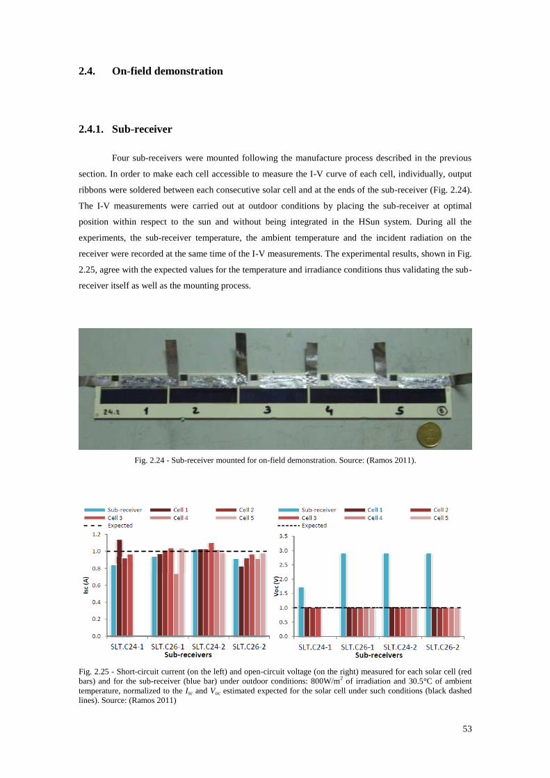
53

2.4. On-field demonstration

2.4.1. Sub-receiver

Four sub-receivers were mounted following the manufacture process described in the previous

section. In order to make each cell accessible to measure the I-V curve of each cell, individually, output

ribbons were soldered between each consecutive solar cell and at the ends of the sub-receiver (Fig. 2.24).

The I-V measurements were carried out at outdoor conditions by placing the sub-receiver at optimal

position within respect to the sun and without being integrated in the HSun system. During all the

experiments, the sub-receiver temperature, the ambient temperature and the incident radiation on the

receiver were recorded at the same time of the I-V measurements. The experimental results, shown in Fig.

2.25, agree with the expected values for the temperature and irradiance conditions thus validating the sub-

receiver itself as well as the mounting process.

Fig. 2.24 - Sub-receiver mounted for on-field demonstration. Source: (Ramos 2011).

Fig. 2.25 - Short-circuit current (on the left) and open-circuit voltage (on the right) measured for each solar cell (red

bars) and for the sub-receiver (blue bar) under outdoor conditions: 800W/m2 of irradiation and 30.5°C of ambient

temperature, normalized to the Isc and Voc estimated expected for the solar cell under such conditions (black dashed

lines). Source: (Ramos 2011)

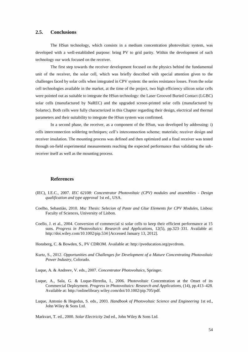
54

2.5. Conclusions

The HSun technology, which consists in a medium concentration photovoltaic system, was

developed with a well-established purpose: bring PV to grid parity. Within the development of such

technology our work focused on the receiver.

The first step towards the receiver development focused on the physics behind the fundamental

unit of the receiver, the solar cell, which was briefly described with special attention given to the

challenges faced by solar cells when integrated in CPV system: the series resistance losses. From the solar

cell technologies available in the market, at the time of the project, two high efficiency silicon solar cells

were pointed out as suitable to integrate the HSun technology: the Laser Grooved Buried Contact (LGBC)

solar cells (manufactured by NaREC) and the upgraded screen-printed solar cells (manufactured by

Solartec). Both cells were fully characterized in this Chapter regarding their design, electrical and thermal

parameters and their suitability to integrate the HSun system was confirmed.

In a second phase, the receiver, as a component of the HSun, was developed by addressing: i)

cells interconnection soldering techniques; cell’s interconnection scheme; materials; receiver design and

receiver insulation. The mounting process was defined and then optimized and a final receiver was tested

through on-field experimental measurements reaching the expected performance thus validating the sub-

receiver itself as well as the mounting process.

References

(IEC), I.E.C., 2007. IEC 62108: Concentrator Photovoltaic (CPV) modules and assemblies - Design

qualification and type approval 1st ed., USA.

Coelho, Sebastião, 2010. Msc Thesis: Selecion of Paste and Glue Elements for CPV Modules, Lisboa:

Faculty of Sciences, University of Lisbon.

Coello, J. et al., 2004. Conversion of commercial si solar cells to keep their efficient performance at 15

suns. Progress in Photovoltaics: Research and Applications, 12(5), pp.323–331. Available at:

http://doi.wiley.com/10.1002/pip.534 [Accessed January 13, 2012].

Honsberg, C. & Bowden, S., PV CDROM. Available at: http://pveducation.org/pvcdrom.

Kurtz, S., 2012. Opportunities and Challenges for Development of a Mature Concentrating Photovoltaic

Power Industry, Colorado.

Luque, A. & Andreev, V. eds., 2007. Concentrator Photovoltaics, Springer.

Luque, A., Sala, G. & Luque-Heredia, I., 2006. Photovoltaic Concentration at the Onset of its

Commercial Deployment. Progress in Photovoltaics: Research and Applications, (14), pp.413–428.

Available at: http://onlinelibrary.wiley.com/doi/10.1002/pip.705/pdf.

Luque, Antonio & Hegedus, S. eds., 2003. Handbook of Photovoltaic Science and Engineering 1st ed.,

John Wiley & Sons Ltd.

Markvart, T. ed., 2000. Solar Electricity 2nd ed., John Wiley & Sons Ltd.

55

Meier, D. & Schroder, D., 1984. Contact resistance: its measurement and relative importance to power

loss in a solar cell. Electron Devices, IEEE Transactions, (5). Available at:

http://ieeexplore.ieee.org/xpls/abs_all.jsp?arnumber=1483869 [Accessed February 9, 2012].

Mendes-Lopes, J. et al., 2011. On-field Demonstration Results of Medium Concentration System

HSUN®. In CPV-7 conference. Las Vegas, USA.

Nelson, J., 2003. The Physics of Solar Cells 1st ed., London: Imperial College Press.

Neuhaus, D.-H. & Münzer, A., 2007. Industrial Silicon Wafer Solar Cells. Advances in OptoElectronics,

2007, pp.1–15. Available at: http://www.hindawi.com/journals/aoe/2007/024521/abs/ [Accessed

March 6, 2013].

Petrova-Koch, V., Hezel, R. & Goetzberger, A. eds., 2009. High-Efficient Low-Cost Photovoltaics 1st ed.,

Springer Series in Optical Sciences.

Ramos, C., 2011. MsC Thesis: Potential of CPV Receivers integrating screen-printed solar cells,

Faculdade de Ciências e Tecnologia, Universidade Nova de Lisboa.

Schroder, D.K., 2006. Semiconductor Materials and Device Characterization 3rd ed., New Jersey: John

Wiley & Sons Ltd.

Serra, J.M., 1995. PhD thesis, University of Lisbon.

Vivar, M. et al., 2010. Laser grooved buried contact cells optimised for linear concentration systems.

Solar Energy Materials and Solar Cells, 94(2), pp.187–193. Available at:

http://linkinghub.elsevier.com/retrieve/pii/S0927024809003079 [Accessed March 7, 2013].

Yordanov, G.H., Midtgard, O.M. & Saetre, T.O., 2010a. Extracting parameters from semi-log plots of

polycrystalline silicon PV modules outdoor I–V data: Double-exponential model revisited. In

Photovoltaic Specialists Conference (PVSC), 2010 35th IEEE. IEEE, pp. 002756–002761.

Available at: http://ieeexplore.ieee.org/xpls/abs_all.jsp?arnumber=5616808 [Accessed January 23,

2012].

Yordanov, G.H., Midtgard, O.M. & Saetre, T.O., 2010b. Two-diode model revisited: parameters

extraction from semi-log plots of I-V data. In 25th European Photovoltaic Solar Energy Conference

and Exhibition / 5th World Conference on Photovoltaic Energy Conversion. Valencia, Spain, pp.

4156 – 4163. Available at: http://onlinelibrary.wiley.com/doi/10.1002/cbdv.200490137/abstract

[Accessed January 13, 2012].

56

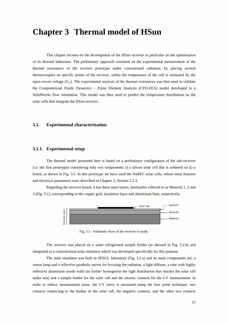
57

Chapter 3 Thermal model of HSun

This chapter focuses on the development of the HSun receiver in particular on the optimization

of its thermal behaviour. The preliminary approach consisted on the experimental measurement of the

thermal resistances of the receiver prototype under concentrated radiation, by placing several

thermocouples on specific points of the receiver, whilst the temperature of the cell is estimated by the

open-circuit voltage (Voc). The experimental analysis of the thermal resistances was then used to validate

the Computational Fluids Dynamics – Finite Element Analysis (CFD-FEA) model developed in a

SolidWorks flow simulation. This model was then used to predict the temperature distribution on the

solar cells that integrate the HSun receiver.

3.1. Experimental characterization

3.1.1. Experimental setup

The thermal model presented here is based on a preliminary configuration of the sub-receiver

(i.e. the first prototype) considering only two components: i) a silicon solar cell that is soldered on ii) a

board, as shown in Fig. 3.1. In this prototype we have used the NaREC solar cells, whose main features

and electrical parameters were described in Chapter 2, Section 2.2.3.

Regarding the receiver board, it has three main layers, hereinafter referred to as Material 1, 2 and

3 (Fig. 3.1), corresponding to the copper grid, insulation layer and aluminium base, respectively.

Fig. 3.1 - Schematic draw of the receiver in study.

The receiver was placed on a water refrigerated sample holder (as showed in Fig. 3.2.b) and

integrated in a concentration solar simulator which was developed specifically for this purpose.

The solar simulator was built in SESUL laboratory (Fig. 3.2.a) and its main components are: a

xenon lamp and a reflective parabolic mirror for focusing the radiation, a light diffuser, a tube with highly

reflective aluminium inside walls (to further homogenise the light distribution that reaches the solar cell

under test) and a sample holder for the solar cell and the electric contacts for the I-V measurement. In

order to reduce measurement noise, the I-V curve is measured using the four point technique: two

contacts connecting to the busbar of the solar cell, the negative contacts, and the other two contacts

58

connecting on the rear side of the cell, positive contacts. The two front (negative) contacts are performed

via two needle-like probes, while the rear (positive) contacts are made by the aluminium sample holder

itself and another point probe. The sample holder has a groove that ensures the vacuum fixation of the cell

and the electric contacts. Such fixation is required to warrant good contact between the cell and the

electric contacts. The sample holder has a water cooling system, which enables the variation of the cell

temperature by turning on or off the water flow that passes through the sample holder. Regarding the

concentration level, this parameter might be adjusted by moving the shelf where the sample holder sits or

by moving it as shown in Fig. 3.2 c).

The experimental setup allows the measurement of the following experimental parameters:

the I-V curve of the cell;

the temperature on the front surface of the receiver, i.e. of Material 1;

the temperature on the rear surface of the receiver, i.e. of Material 3;

the temperature on the rear surface of the sample holder;

the temperature in the solar simulator chamber; and

the temperature of the water flow.

a) b)

c)

Fig. 3.2 - Solar simulador: a) build at SESUL laboratory; b) schematic representation of the solar simulator; and c)

detail of the sample holder integrated in the solar simulator.

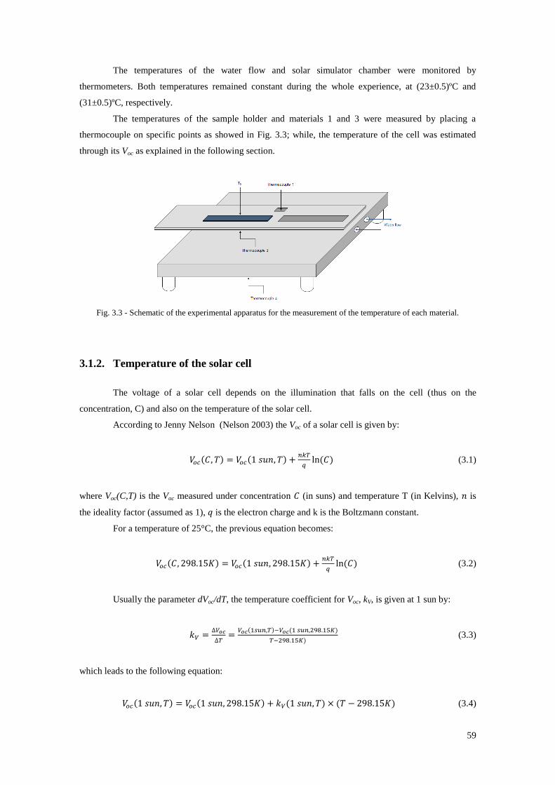
59

The temperatures of the water flow and solar simulator chamber were monitored by

thermometers. Both temperatures remained constant during the whole experience, at (23±0.5)ºC and

(31±0.5)ºC, respectively.

The temperatures of the sample holder and materials 1 and 3 were measured by placing a

thermocouple on specific points as showed in Fig. 3.3; while, the temperature of the cell was estimated

through its Voc as explained in the following section.

Fig. 3.3 - Schematic of the experimental apparatus for the measurement of the temperature of each material.

3.1.2. Temperature of the solar cell

The voltage of a solar cell depends on the illumination that falls on the cell (thus on the

concentration, C) and also on the temperature of the solar cell.

According to Jenny Nelson (Nelson 2003) the Voc of a solar cell is given by:

( ) ( )

( ) (3.1)

where Voc(C,T) is the Voc measured under concentration (in suns) and temperature T (in Kelvins), is

the ideality factor (assumed as 1), is the electron charge and k is the Boltzmann constant.

For a temperature of 25°C, the previous equation becomes:

( ) ( )

( ) (3.2)

Usually the parameter dVoc/dT, the temperature coefficient for Voc, kV, is given at 1 sun by:

( ) ( )

) (3.3)

which leads to the following equation:

( ) ( ) ( ) ( ) (3.4)

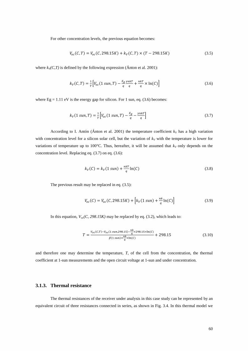
60

For other concentration levels, the previous equation becomes:

( ) ( ) ( ) ( ) (3.5)

where kV(C,T) is defined by the following expression (Ánton et al. 2001):

( )

[ ( )

( )] (3.6)

where Eg = 1.11 eV is the energy gap for silicon. For 1 sun, eq. (3.6) becomes:

( )

[ ( )

] (3.7)

According to I. Antón (Ánton et al. 2001) the temperature coefficient kV has a high variation

with concentration level for a silicon solar cell, but the variation of kV with the temperature is lower for

variations of temperature up to 100°C. Thus, hereafter, it will be assumed that kV only depends on the

concentration level. Replacing eq. (3.7) on eq. (3.6):

( ) ( )

( ) (3.8)

The previous result may be replaced in eq. (3.5):

( ) ( ) [ ( )

( )] (3.9)

In this equation, Voc(C, 298.15K) may be replaced by eq. (3.2), which leads to:

( ) ( )

( )

( )

( )

(3.10)

and therefore one may determine the temperature, T, of the cell from the concentration, the thermal

coefficient at 1-sun measurements and the open circuit voltage at 1-sun and under concentration.

3.1.3. Thermal resistance

The thermal resistances of the receiver under analysis in this case study can be represented by an

equivalent circuit of three resistances connected in series, as shown in Fig. 3.4. In this thermal model we

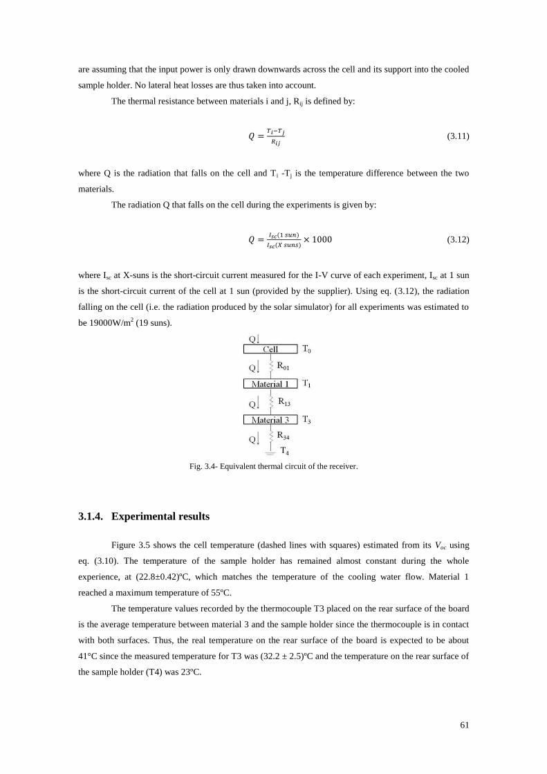
61

are assuming that the input power is only drawn downwards across the cell and its support into the cooled

sample holder. No lateral heat losses are thus taken into account.

The thermal resistance between materials i and j, Rij is defined by:

(3.11)

where Q is the radiation that falls on the cell and Ti -Tj is the temperature difference between the two

materials.

The radiation Q that falls on the cell during the experiments is given by:

( )

( ) (3.12)

where Isc at X-suns is the short-circuit current measured for the I-V curve of each experiment, Isc at 1 sun

is the short-circuit current of the cell at 1 sun (provided by the supplier). Using eq. (3.12), the radiation

falling on the cell (i.e. the radiation produced by the solar simulator) for all experiments was estimated to

be 19000W/m2 (19 suns).

Fig. 3.4- Equivalent thermal circuit of the receiver.

3.1.4. Experimental results

Figure 3.5 shows the cell temperature (dashed lines with squares) estimated from its Voc using

eq. (3.10). The temperature of the sample holder has remained almost constant during the whole

experience, at (22.8±0.42)ºC, which matches the temperature of the cooling water flow. Material 1

reached a maximum temperature of 55ºC.

The temperature values recorded by the thermocouple T3 placed on the rear surface of the board

is the average temperature between material 3 and the sample holder since the thermocouple is in contact

with both surfaces. Thus, the real temperature on the rear surface of the board is expected to be about

41°C since the measured temperature for T3 was (32.2 ± 2.5)ºC and the temperature on the rear surface of

the sample holder (T4) was 23ºC.

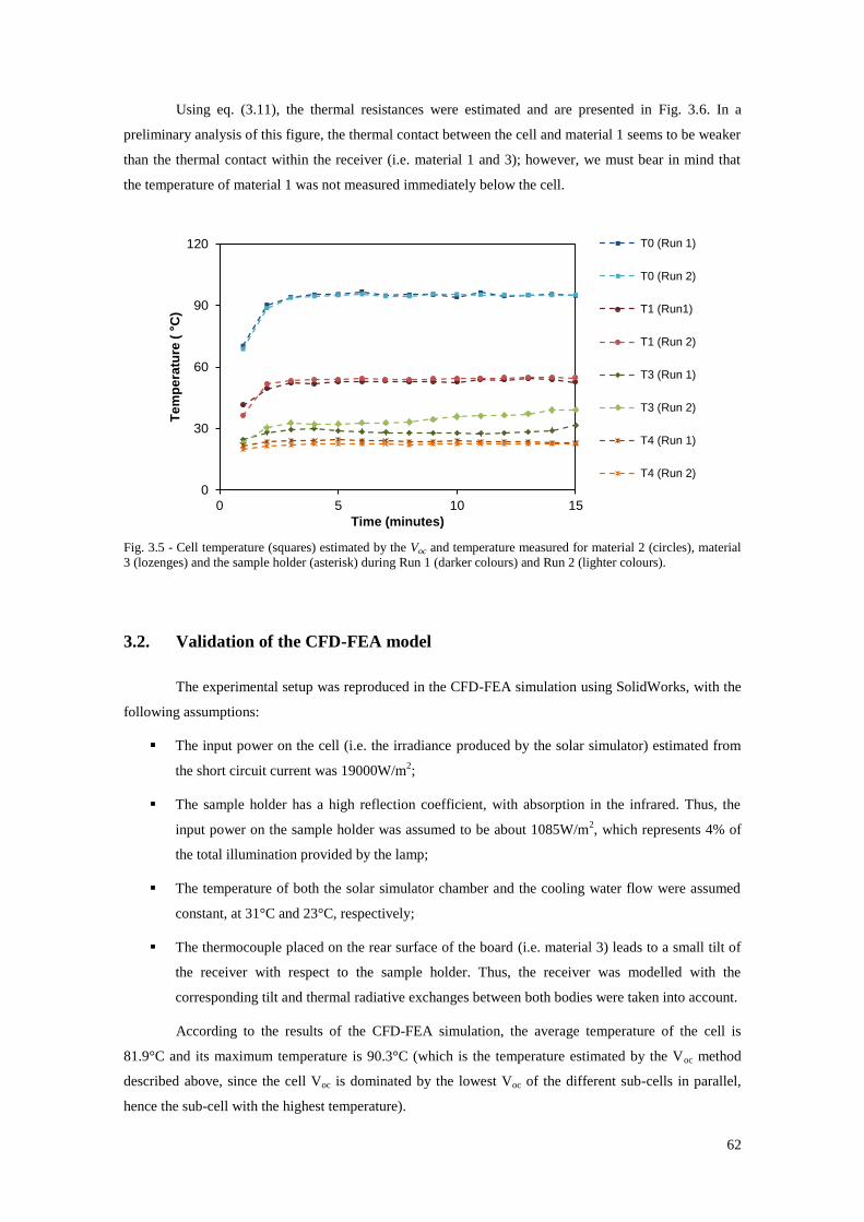
62

Using eq. (3.11), the thermal resistances were estimated and are presented in Fig. 3.6. In a

preliminary analysis of this figure, the thermal contact between the cell and material 1 seems to be weaker

than the thermal contact within the receiver (i.e. material 1 and 3); however, we must bear in mind that

the temperature of material 1 was not measured immediately below the cell.

Fig. 3.5 - Cell temperature (squares) estimated by the Voc and temperature measured for material 2 (circles), material

3 (lozenges) and the sample holder (asterisk) during Run 1 (darker colours) and Run 2 (lighter colours).

3.2. Validation of the CFD-FEA model

The experimental setup was reproduced in the CFD-FEA simulation using SolidWorks, with the

following assumptions:

The input power on the cell (i.e. the irradiance produced by the solar simulator) estimated from

the short circuit current was 19000W/m2;

The sample holder has a high reflection coefficient, with absorption in the infrared. Thus, the

input power on the sample holder was assumed to be about 1085W/m2, which represents 4% of

the total illumination provided by the lamp;

The temperature of both the solar simulator chamber and the cooling water flow were assumed

constant, at 31°C and 23°C, respectively;

The thermocouple placed on the rear surface of the board (i.e. material 3) leads to a small tilt of

the receiver with respect to the sample holder. Thus, the receiver was modelled with the

corresponding tilt and thermal radiative exchanges between both bodies were taken into account.

According to the results of the CFD-FEA simulation, the average temperature of the cell is

81.9°C and its maximum temperature is 90.3°C (which is the temperature estimated by the Voc method

described above, since the cell Voc is dominated by the lowest Voc of the different sub-cells in parallel,

hence the sub-cell with the highest temperature).

0

30

60

90

120

0 5 10 15

Te

mp

era

ture

( °

C)

Time (minutes)

T0 (Run 1)

T0 (Run 2)

T1 (Run1)

T1 (Run 2)

T3 (Run 1)

T3 (Run 2)

T4 (Run 1)

T4 (Run 2)

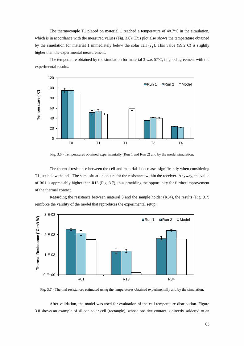
63

The thermocouple T1 placed on material 1 reached a temperature of 48.7°C in the simulation,

which is in accordance with the measured values (Fig. 3.6). This plot also shows the temperature obtained

by the simulation for material 1 immediately below the solar cell ( ). This value (59.2°C) is slightly

higher than the experimental measurement.

The temperature obtained by the simulation for material 3 was 57ºC, in good agreement with the

experimental results.

Fig. 3.6 - Temperatures obtained experimentally (Run 1 and Run 2) and by the model simulation.

The thermal resistance between the cell and material 1 decreases significantly when considering

T1 just below the cell. The same situation occurs for the resistance within the receiver. Anyway, the value

of R01 is appreciably higher than R13 (Fig. 3.7), thus providing the opportunity for further improvement

of the thermal contact.

Regarding the resistance between material 3 and the sample holder (R34), the results (Fig. 3.7)

reinforce the validity of the model that reproduces the experimental setup.

Fig. 3.7 - Thermal resistances estimated using the temperatures obtained experimentally and by the simulation.

After validation, the model was used for evaluation of the cell temperature distribution. Figure

3.8 shows an example of silicon solar cell (rectangle), whose positive contact is directly soldered to an

0

20

40

60

80

100

120

T0 T1 T1' T3 T4

Te

mp

era

ture

(°C

)

Run 1 Run 2 Model

0.E+00

1.E-03

2.E-03

3.E-03

R01 R13 R34

Th

erm

al R

es

ista

nc

e (°C

m2/

W)

Run 1 Run 2 Model

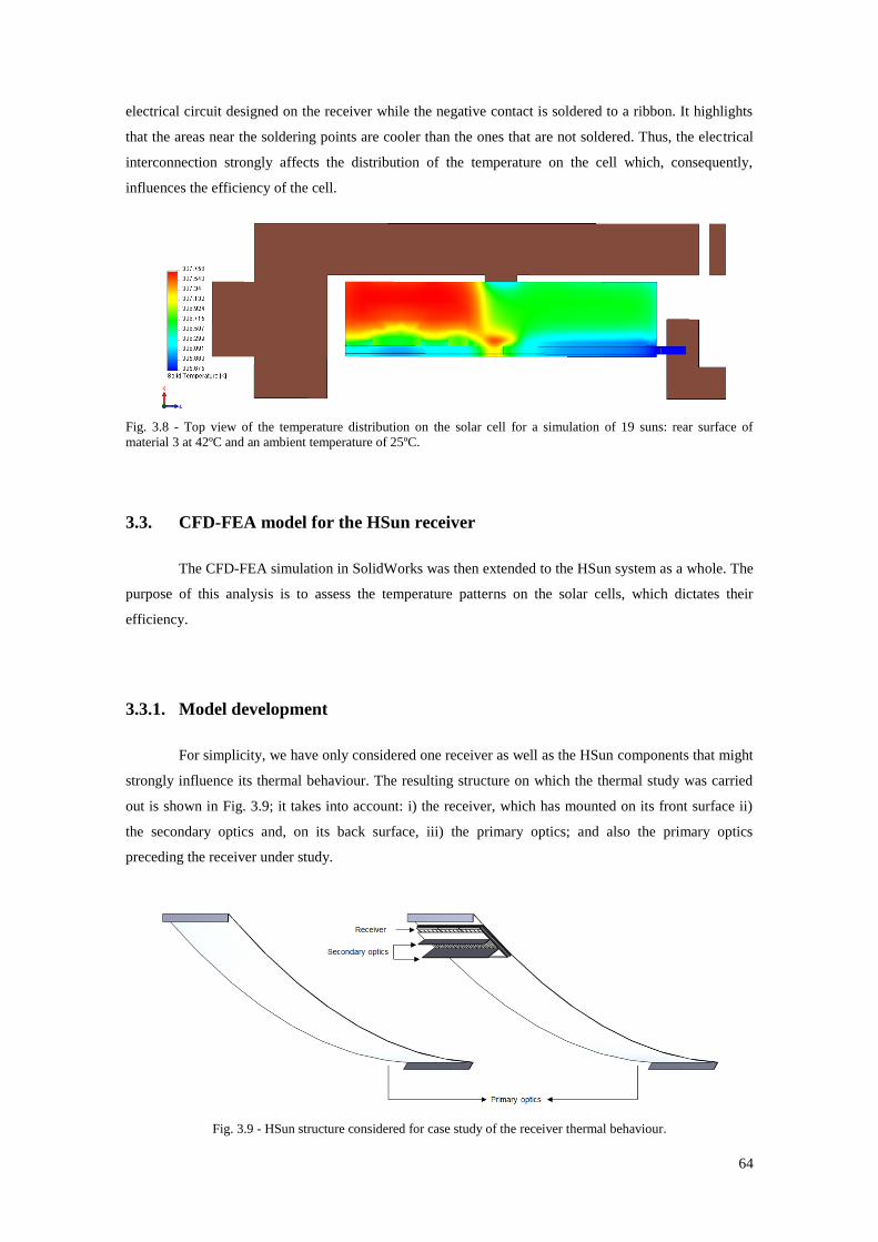
64

electrical circuit designed on the receiver while the negative contact is soldered to a ribbon. It highlights

that the areas near the soldering points are cooler than the ones that are not soldered. Thus, the electrical

interconnection strongly affects the distribution of the temperature on the cell which, consequently,

influences the efficiency of the cell.

Fig. 3.8 - Top view of the temperature distribution on the solar cell for a simulation of 19 suns: rear surface of

material 3 at 42ºC and an ambient temperature of 25ºC.

3.3. CFD-FEA model for the HSun receiver

The CFD-FEA simulation in SolidWorks was then extended to the HSun system as a whole. The

purpose of this analysis is to assess the temperature patterns on the solar cells, which dictates their

efficiency.

3.3.1. Model development

For simplicity, we have only considered one receiver as well as the HSun components that might

strongly influence its thermal behaviour. The resulting structure on which the thermal study was carried

out is shown in Fig. 3.9; it takes into account: i) the receiver, which has mounted on its front surface ii)

the secondary optics and, on its back surface, iii) the primary optics; and also the primary optics

preceding the receiver under study.

Fig. 3.9 - HSun structure considered for case study of the receiver thermal behaviour.

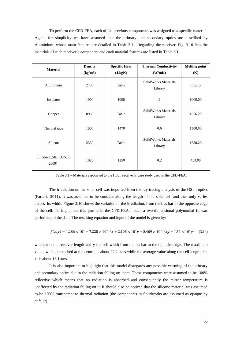
65

To perform the CFD-FEA, each of the previous components was assigned to a specific material.

Again, for simplicity we have assumed that the primary and secondary optics are described by

Aluminium, whose main features are detailed in Table 3.1. Regarding the receiver, Fig. 3.10 lists the

materials of each receiver’s component and each material features are listed in Table 3.1.

Material Density

(kg/m3)

Specific Heat

(J/kgK)

Thermal Conductivity

(W/mK)

Melting point

(K)

Aluminium 2700 Table SolidWorks Materials

Library 855.15

Insulator 1000 1000 2 1000.00

Copper 8960 Table SolidWorks Materials

Library 1356.20

Thermal tape 1500 1470 0.6 1500.00

Silicon 2330 Table SolidWorks Materials

Library 1688.20

Silicone [(SILICONES

2009)] 1020 1250 0.2 453.00

Table 3.1 – Materials associated to the HSun receiver’s case study used in the CFD-FEA.

The irradiation on the solar cell was imported from the ray tracing analysis of the HSun optics

(Fartaria 2011). It was assumed to be constant along the length of the solar cell and thus only varies

across its width. Figure 3.10 shows the variation of the irradiation, from the bus bar to the opposite edge

of the cell. To implement this profile in the CFD-FEA model, a two-dimensional polynomial fit was

performed to the data. The resulting equation and input of the model is given by:

( ) (3.14)

where is the receiver length and the cell width from the busbar to the opposite edge. The maximum

value, which is reached at the centre, is about 22.2 suns while the average value along the cell length, i.e.

x, is about 18.1suns.

It is also important to highlight that this model disregards any possible warming of the primary

and secondary optics due to the radiation falling on them. These components were assumed to be 100%

reflective which means that no radiation is absorbed and consequently the mirror temperature is

unaffected by the radiation falling on it. It should also be noticed that the silicone material was assumed

to be 100% transparent to thermal radiation (the components in Solidworks are assumed as opaque by

default).

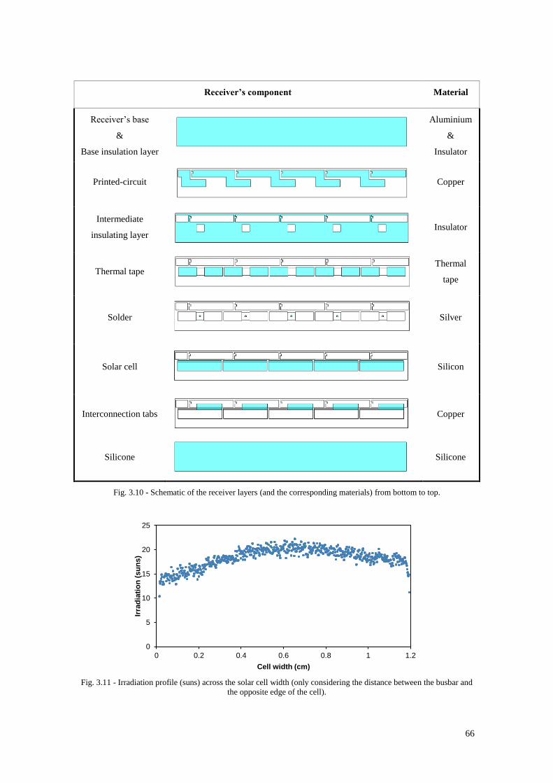
66

Receiver’s component Material

Receiver’s base

&

Base insulation layer

Aluminium

&

Insulator

Printed-circuit

Copper

Intermediate

insulating layer

Insulator

Thermal tape

Thermal

tape

Solder

Silver

Solar cell

Silicon

Interconnection tabs

Copper

Silicone

Silicone

Fig. 3.10 - Schematic of the receiver layers (and the corresponding materials) from bottom to top.

Fig. 3.11 - Irradiation profile (suns) across the solar cell width (only considering the distance between the busbar and

the opposite edge of the cell).

0

5

10

15

20

25

0 0.2 0.4 0.6 0.8 1 1.2

Irra

dia

tio

n (

su

ns

)

Cell width (cm)

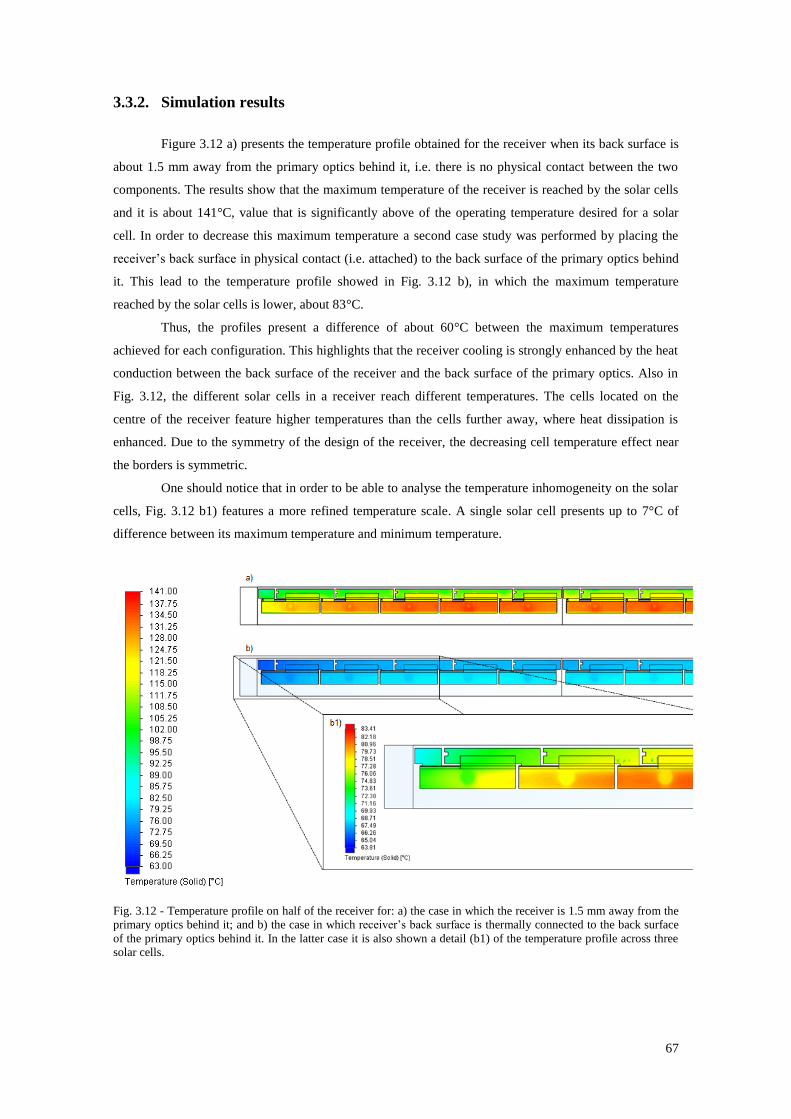
67

3.3.2. Simulation results

Figure 3.12 a) presents the temperature profile obtained for the receiver when its back surface is

about 1.5 mm away from the primary optics behind it, i.e. there is no physical contact between the two

components. The results show that the maximum temperature of the receiver is reached by the solar cells

and it is about 141°C, value that is significantly above of the operating temperature desired for a solar

cell. In order to decrease this maximum temperature a second case study was performed by placing the

receiver’s back surface in physical contact (i.e. attached) to the back surface of the primary optics behind

it. This lead to the temperature profile showed in Fig. 3.12 b), in which the maximum temperature

reached by the solar cells is lower, about 83°C.

Thus, the profiles present a difference of about 60°C between the maximum temperatures

achieved for each configuration. This highlights that the receiver cooling is strongly enhanced by the heat

conduction between the back surface of the receiver and the back surface of the primary optics. Also in

Fig. 3.12, the different solar cells in a receiver reach different temperatures. The cells located on the

centre of the receiver feature higher temperatures than the cells further away, where heat dissipation is

enhanced. Due to the symmetry of the design of the receiver, the decreasing cell temperature effect near

the borders is symmetric.

One should notice that in order to be able to analyse the temperature inhomogeneity on the solar

cells, Fig. 3.12 b1) features a more refined temperature scale. A single solar cell presents up to 7°C of

difference between its maximum temperature and minimum temperature.

Fig. 3.12 - Temperature profile on half of the receiver for: a) the case in which the receiver is 1.5 mm away from the

primary optics behind it; and b) the case in which receiver’s back surface is thermally connected to the back surface

of the primary optics behind it. In the latter case it is also shown a detail (b1) of the temperature profile across three

solar cells.

68

3.4. Conclusions

The preliminary version of the CFD-FEA model presented in this Chapter has shown good

agreement with the experimental results, thus reinforcing its potential to be used as a decision tool for the

development of the CPV receiver.

The CFD-FEA model of the receiver was extended for the whole HSun concept design. The

simulation results have shown that:

the primary optics play an important role on the receiver cooling since it may decrease the solar

cells temperature by about 58°C;

the solar cells on the receiver reach different average temperatures which will certainly put

some constraints on the receiver efficiency; and

the solar cells individually feature an inhomogeneous distribution of temperature. This latter

point highlights the need for careful analysis of the effect of the temperature profile on the performance of

the solar cells. This is the aim of the discussion in the following chapters.

References

Ánton, I., Sala, G. & Pachón, D., 2001. Correction of the Voc vs. temperature dependence under non-

uniform concentrated illumination. In Proceedings of the 17th European Photovoltaic Solar Energy

Conference. Munich, p. 156.

Fartaria, T., 2011. Tolerance Study and Optical Optimization of a Concentrated Photovoltaic Module.,

Instituto Superior Técnico, Universidade Técnica de Lisboa.

Nelson, J., 2003. The Physics of Solar Cells 1st ed., London, UK: Imperial College Press.

SILICONES, W., 2009. ELASTOSIL RT 601.

69

Chapter 4 Modelling CPV silicon solar cells

High efficiency silicon solar cells with low series resistance are useful for low and medium

concentration photovoltaic (CPV) systems, such as the HSun concept. However, unlike standard flat-plate

systems, usually the optics of solar concentrator photovoltaic systems exhibits an inhomogeneous

illumination profile along the solar cell surface. Such inhomogeneity may be further amplified by

structure and tracking misalignments, which may possibly occur during manufacturing and mounting

processes or even during its lifetime (Luque et al. 1998).

The illumination profile influences the distribution of current and temperature in the solar cell

thus modifying the ohmic losses and, consequently, its I-V curve (Luque et al. 1998; Mellor et al. 2009;

ET Franklin & J. Coventry 2002). Such effects are only carelessly reproduced by standard solar cell

models which include an equivalent lumped series resistance and the cell equivalent circuit (Luque et al.

1998; Mellor et al. 2009; ET Franklin & J. Coventry 2002). For an accurate estimation of the solar cells

output when integrated in CPV systems under inhomogeneous illumination and temperature profiles it is

crucial that the electrical solar cell model takes into account the ‘distributed diode effect’(ET Franklin &

J. Coventry 2002; Mitchell 1977). In this chapter we describe the development of an electrical model that

takes into account such effect. This chapter includes a detailed literature review of the distributed diode

effect modelling and a general description of the model. The following chapters will describe the model

implementation, experimental validation for both illumination and temperature homogeneous and

inhomogeneous profiles, analysis and, finally, the highly significance of the model will appear when it is

extended to an optimization tool that suggest the appropriate pattern for the front grid contact taking into

account the illumination an temperature profiles on the cell.

4.1. Introduction

Concentration Photovoltaic (CPV) systems generally exhibit a non-uniform illumination profile

along the solar cells they integrate (Mitchell 1977; Luque et al. 1998; ET Franklin & J. Coventry 2002;

Mellor et al. 2009). The light distribution in such profiles is defined by the design of the concentrator

optics and is influenced by structure, optics and tracking misalignments, which possibly occur during

manufacturing/mounting processes or even during its lifetime (Luque et al. 1998). The resulting

illumination profile on the CPV cells will influence the distribution of current in these devices thus

modifying its ohmic losses and, consequently, its I-V curve (ET Franklin & J. Coventry 2002; Luque et

al. 1998; Mellor et al. 2009; Joe S. Coventry 2005).

On the other hand, the illumination profile will also dictate the temperature profile on those cells

since the highly illuminated cell regions are susceptible to become warmer than the ones poorly

illuminated (Joe S. Coventry 2005). Furthermore, in the CPV solar cells, the amount of radiation that

reaches the cell is considerably high, which is the reason why most of the CPV systems usually integrate

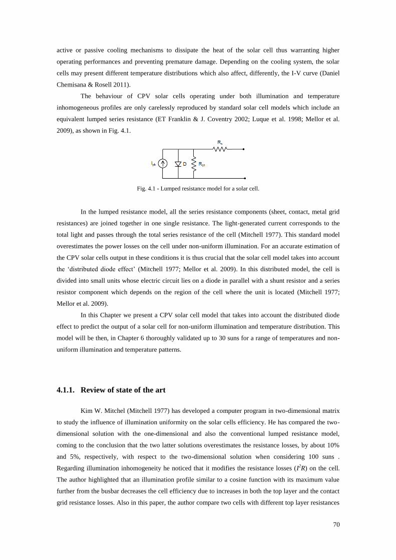
70

active or passive cooling mechanisms to dissipate the heat of the solar cell thus warranting higher

operating performances and preventing premature damage. Depending on the cooling system, the solar

cells may present different temperature distributions which also affect, differently, the I-V curve (Daniel

Chemisana & Rosell 2011).

The behaviour of CPV solar cells operating under both illumination and temperature

inhomogeneous profiles are only carelessly reproduced by standard solar cell models which include an

equivalent lumped series resistance (ET Franklin & J. Coventry 2002; Luque et al. 1998; Mellor et al.

2009), as shown in Fig. 4.1.

Fig. 4.1 - Lumped resistance model for a solar cell.

In the lumped resistance model, all the series resistance components (sheet, contact, metal grid

resistances) are joined together in one single resistance. The light-generated current corresponds to the

total light and passes through the total series resistance of the cell (Mitchell 1977). This standard model

overestimates the power losses on the cell under non-uniform illumination. For an accurate estimation of

the CPV solar cells output in these conditions it is thus crucial that the solar cell model takes into account

the ‘distributed diode effect’ (Mitchell 1977; Mellor et al. 2009). In this distributed model, the cell is

divided into small units whose electric circuit lies on a diode in parallel with a shunt resistor and a series

resistor component which depends on the region of the cell where the unit is located (Mitchell 1977;

Mellor et al. 2009).

In this Chapter we present a CPV solar cell model that takes into account the distributed diode

effect to predict the output of a solar cell for non-uniform illumination and temperature distribution. This

model will be then, in Chapter 6 thoroughly validated up to 30 suns for a range of temperatures and non-

uniform illumination and temperature patterns.

4.1.1. Review of state of the art

Kim W. Mitchel (Mitchell 1977) has developed a computer program in two-dimensional matrix

to study the influence of illumination uniformity on the solar cells efficiency. He has compared the two-

dimensional solution with the one-dimensional and also the conventional lumped resistance model,

coming to the conclusion that the two latter solutions overestimates the resistance losses, by about 10%

and 5%, respectively, with respect to the two-dimensional solution when considering 100 suns .

Regarding illumination inhomogeneity he noticed that it modifies the resistance losses (I2R) on the cell.

The author highlighted that an illumination profile similar to a cosine function with its maximum value

further from the busbar decreases the cell efficiency due to increases in both the top layer and the contact

grid resistance losses. Also in this paper, the author compare two cells with different top layer resistances

71

concluding that for the low top layer resistance cell, the cosine-like illumination has negligible effect

below 100 suns, with a power loss less than 2% even at 500 suns.

C. M. Garner and R. D. Nasby (Garner & Nsaby 1979) developed a two-dimensional computer

code which solves Poisson’s equation for each point of the grid and estimates the I-V characteristic. The

model was checked against experimental results for known stepwise illumination profiles. They

concluded that the series resistance losses for non-uniform illumination with its peak at the centre of the

cell are higher than those under uniform illumination; moreover, cell efficiencies for the non-uniform

illumination profiles have a maximum at lower concentrations and then decrease with increasing

concentration.

H. Pfeiffer and M. Bihler (Pfeiffer & Bihler 1982) have experimentally investigated the effects

of non-uniform illumination by placing strip filters of 1mm with different transmission factors on the

outer edges of a solar cell, an illumination profile representative of many CPV systems. The studies were

carried out with a solar simulator at light intensity of 9 suns showing that the measured power loss of

output resulting from non-uniform illumination stands below 3%. The investigation was extended to

evaluate the influence of different geometries and positions of the strip filters with respect to the cell

surface. The results showed no detectable relation between these different configurations and cell output,

a statement which is in agreement with Garner et al. (Garner & Nsaby 1979).

A. Cuevas and S. López-Romero (Cuevas & López-Romero 1984) highlight in their paper that

most of the experiments that were carried out to study the effect of inhomogeneous illumination until that

time were performed with concentrator solar cells, whose series resistance (Rs) are typically very low thus

softening, in particular, the decrease in Voc. This way, the authors proposed to study experimentally the

effect of harshly non-uniform illumination on the I-V curve of two extreme cells: i) one with very low Rs,

representative of concentrator solar cells; and another one ii) with very high Rs, representative of standard

solar cells. They came to the conclusion that the series resistance affects cell’s Voc if it is non-uniformly

illuminated; moreover, the decrease in Voc can be very significant in cases of high series resistance, non-

uniformity and relatively high irradiance. The authors also highlighted that if the irradiance is increased

over the normal operation irradiance level, some unavoidable metal grid shadows, and consequently non-

uniform illumination, may arise thus decreasing the Voc. Such effect is even more noticeable with the non-

uniform illumination pattern formed by the concentrator optics.

A. Luque, G. Sala and J. C. Arboiro (Luque et al. 1998) developed a thermal and electric model

to study the influence of stepwise inhomogeneous illumination on the temperature distribution of the CPV

receiver and its electrical performance. The models were checked against EUCLIDES concentrator

(Luque et al. 1998) experimental behaviour, showing good agreement. Regarding thermal effects, the

authors highlight that strong local heating arises when the cells are operating under inhomogeneous

illumination and it can lead to an increase in cell temperature when compared to the case of homogeneous

illumination. This effect is also included in the electrical model and along with an increase in the series

resistance losses leads to an efficiency drop under non-uniform illumination profiles; however, such drop

is lower than expected since poorer parts of the solar cell are switched off.

E. T. Franklin and J. S. Coventry (ET Franklin & J. Coventry 2002) developed a model to study

the effect of a Gaussian illumination profile on solar cells which corresponds to the illumination profile

72

found on the CHAPS system (Joe S. Coventry 2005; J S Coventry et al. 2004). For the model, the cell is

divided into quarter finger-space units, which are represented by a single diode equation whose series

resistance is divided in the bulk, emitter, finger and contact components. Local temperature, i.e. the

temperature of the cell unit, is also considered in the model. The entire cell behaviour is finally obtained

by accumulation of identical units. The model was used to compare different degrees of centralized

illumination, maintaining the average irradiation on the cell at 30 suns; this revealed that an increasingly

centralized Gaussian illumination may lead to larger decrease in Voc and efficiency. Regarding

experimental validation it was only addressed through stepwise illumination, thus only allowing a

qualitative comparison with the model results obtained for Gaussian profiles.

Ahmed E. Ghitas and M. Sabry (Ghitas & Sabry 2006; Sabry & Ghitas 2006) addressed

experimentally the effects of inhomogeneous irradiation measuring the I-V curves at STC on

conventional solar cells partially shaded. First (Sabry & Ghitas 2006), edge shading was addressed by

laying opaque strips on the outer edges of the cell. The I-V curve measurements were performed for

different strip widths and cell temperatures. The main conclusion was that increasing edge shading leads

to a sharp increase in the cell voltage followed by a gradual decrease. Such situation may be justified by

de-activation of the cell border area, where high rate of recombination and, consequently, some shunt

resistance may be found. A reverse behaviour was observed on the Isc, which lead the authors to conclude

that conventional lumped cell models are insufficient to accurately describe the behaviour of solar cells

under edge shading. Moreover, it was also observed that such behaviours are temperature independent. In

a second study (Ghitas & Sabry 2006), the authors compare central cell shadowing with edge cell

shadowing, again through experimental work. They came to the conclusion that both central and edge

shading have negative effects on the cell efficiency; though, the latter has higher effect only in the case of

very thin strips.

A. Mellor, J. L. Domenech-Garret, D.Chemisana, J. I. Rosell (Mellor et al. 2009) developed a

two-dimensional finite element model of current flow in the front surface of the cell taking into account

the distributed diode effect. The model relies on a new method (Rosell & Ibáñez 2006) based on the

adjustment of the slightly modified conventional I-V curve model with a new maximum power output

expression. The parameters for adjustment were obtained from measurements taken under homogeneous

irradiation. The model assumes as domain an entire finger space unit and the temperature is considered

uniform across the cell. Model implementation was performed using ComSol©, which allows the internal

running of SPICE models. Finite Element Method was used to obtain the solutions. The model was used

to demonstrate the reduction in FF and Voc as a result of non-uniform illumination Gaussian profiles in

the finger direction, a typical profile for linear CPV systems. Validation was addressed through

experimental tests, being carried out by using an indoor light concentrator device (6.9 suns) and Gaussian

filters were used to create non-uniform patterns on the cell under. Also in the same work, the authors have

used the model to demonstrate that the effects of Gaussian illumination profiles may be attenuated by re-

optimization of the front grid contact. This study leads to the conclusion that the fill factor may be

improved if the number of fingers increases with increasing peak accentuation.

J. L. Domenech-Garret (J.-L. Domenech-Garret 2011) follows the same cell modelling

framework as in the previous paper; but, in this work the author extended the study to combined profiles

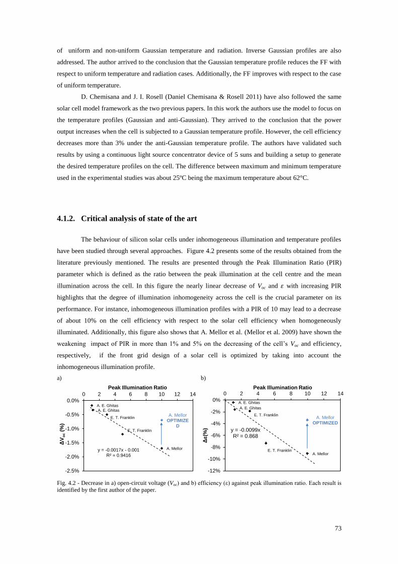
73

of uniform and non-uniform Gaussian temperature and radiation. Inverse Gaussian profiles are also

addressed. The author arrived to the conclusion that the Gaussian temperature profile reduces the FF with

respect to uniform temperature and radiation cases. Additionally, the FF improves with respect to the case

of uniform temperature.

D. Chemisana and J. I. Rosell (Daniel Chemisana & Rosell 2011) have also followed the same

solar cell model framework as the two previous papers. In this work the authors use the model to focus on

the temperature profiles (Gaussian and anti-Gaussian). They arrived to the conclusion that the power

output increases when the cell is subjected to a Gaussian temperature profile. However, the cell efficiency

decreases more than 3% under the anti-Gaussian temperature profile. The authors have validated such

results by using a continuous light source concentrator device of 5 suns and building a setup to generate

the desired temperature profiles on the cell. The difference between maximum and minimum temperature

used in the experimental studies was about 25ºC being the maximum temperature about 62°C.

4.1.2. Critical analysis of state of the art

The behaviour of silicon solar cells under inhomogeneous illumination and temperature profiles

have been studied through several approaches. Figure 4.2 presents some of the results obtained from the

literature previously mentioned. The results are presented through the Peak Illumination Ratio (PIR)

parameter which is defined as the ratio between the peak illumination at the cell centre and the mean

illumination across the cell. In this figure the nearly linear decrease of Voc and with increasing PIR

highlights that the degree of illumination inhomogeneity across the cell is the crucial parameter on its

performance. For instance, inhomogeneous illumination profiles with a PIR of 10 may lead to a decrease

of about 10% on the cell efficiency with respect to the solar cell efficiency when homogeneously

illuminated. Additionally, this figure also shows that A. Mellor et al. (Mellor et al. 2009) have shown the

weakening impact of PIR in more than 1% and 5% on the decreasing of the cell’s Voc and efficiency,

respectively, if the front grid design of a solar cell is optimized by taking into account the

inhomogeneous illumination profile.

a) b)

Fig. 4.2 - Decrease in a) open-circuit voltage (Voc) and b) efficiency (ε) against peak illumination ratio. Each result is

identified by the first author of the paper.

E. T. Franklin

E. T. Franklin

A. E. Ghitas

A. E. Ghitas

A. Mellor

A. Mellor OPTIMIZE

D

y = -0.0017x - 0.001 R² = 0.9416

-2.5%

-2.0%

-1.5%

-1.0%

-0.5%

0.0%

0 2 4 6 8 10 12 14

ΔV

oc (

%)

Peak Illumination Ratio

E. T. Franklin

E. T. Franklin

A. E. Ghitas

A. E. Ghitas

A. Mellor

A. Mellor OPTIMIZED

y = -0.0099x R² = 0.868

-12%

-10%

-8%

-6%

-4%

-2%

0%

0 2 4 6 8 10 12 14

Δε(%

)

Peak Illumination Ratio

74

These results have reinforced the importance of developing a model, thus in this Chapter a 1D

solar cell model that takes into account the distributed diode effect is presented. The model ought to

consider the ‘distributed diode effect’ and was developed in a Matlab/Simulink application based on a

modular structure whose features are easily modified thus allowing suitability for application in any cell

design. Notice that the model presented in this Chapter may be straightforwardly transformed in a 2D

model; however, due to the geometry of the cell and the illumination and temperature ranges this

computing time-consuming approach is unnecessary.

In the next section we propose a model which was built as general as possible in order to be

useful for any CPV systems that integrate silicon solar cells or even to study the effect of partial shading

in conventional flat-plate systems.

4.2. Model

The main purpose of the electrical model presented in this section is to predict the output of a

solar cell for an illumination profile and a well-defined temperature distribution.

In the electrical model, the cell is divided in small units which are considered to be connected in

parallel. The number of units and its location on the cell allows the model to simulate almost any solar

cell configuration. Each unit has a specific resistance (emitter, contact, finger, busbar, bulk etc…)

depending on its position in the cell. The main input parameters for each element are the input radiation

and temperature of that element.

4.3. Cell design

As a case study and without loss of generality, the model was developed to simulate a single-

junction crystalline Si solar cell whose electric contacts design consists of: i) a linear front grid pattern of

parallel fingers that are orthogonal to one lateral busbar as shown in Fig. 4.3.a); and ii) a back contact that

covers the whole rear surface of the solar cell. In the same figure, the nomenclature is (notice that all the

dimensions are defined in cm):

• W - cell width (dimension perpendicular to the busbar);

• L - cell length (dimension parallel to the busbar);

• β - busbar width;

• Z - busbar/ finger thickness;

• d - space between fingers; and

• ω - finger width.

In the model, the solar cell is seen as divided into several similar elements. Each element

encompasses half of one finger width and half of the emitter area that is between two successive fingers

as shown in Fig.4.3.a) by the red dashed line. The total number of elements, f, defines the cell length and

is used by the model algorithm to stop the simulation.

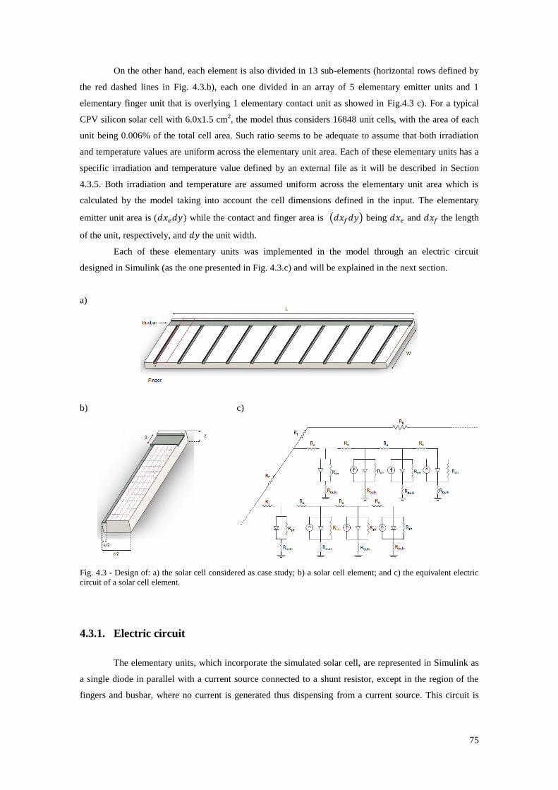
75

On the other hand, each element is also divided in 13 sub-elements (horizontal rows defined by

the red dashed lines in Fig. 4.3.b), each one divided in an array of 5 elementary emitter units and 1

elementary finger unit that is overlying 1 elementary contact unit as showed in Fig.4.3 c). For a typical

CPV silicon solar cell with 6.0x1.5 cm2, the model thus considers 16848 unit cells, with the area of each

unit being 0.006% of the total cell area. Such ratio seems to be adequate to assume that both irradiation

and temperature values are uniform across the elementary unit area. Each of these elementary units has a

specific irradiation and temperature value defined by an external file as it will be described in Section

4.3.5. Both irradiation and temperature are assumed uniform across the elementary unit area which is

calculated by the model taking into account the cell dimensions defined in the input. The elementary

emitter unit area is ( while the contact and finger area is ( ) being and the length

of the unit, respectively, and the unit width.

Each of these elementary units was implemented in the model through an electric circuit

designed in Simulink (as the one presented in Fig. 4.3.c) and will be explained in the next section.

a)

b)

c)

Fig. 4.3 - Design of: a) the solar cell considered as case study; b) a solar cell element; and c) the equivalent electric

circuit of a solar cell element.

4.3.1. Electric circuit

The elementary units, which incorporate the simulated solar cell, are represented in Simulink as

a single diode in parallel with a current source connected to a shunt resistor, except in the region of the

fingers and busbar, where no current is generated thus dispensing from a current source. This circuit is

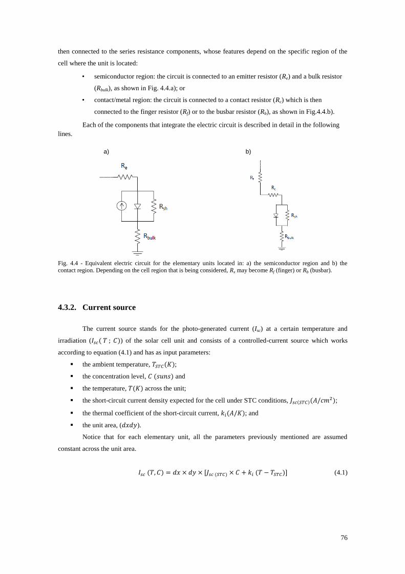
76

then connected to the series resistance components, whose features depend on the specific region of the

cell where the unit is located:

• semiconductor region: the circuit is connected to an emitter resistor (Re) and a bulk resistor

(Rbulk), as shown in Fig. 4.4.a); or

• contact/metal region: the circuit is connected to a contact resistor (Rc) which is then

connected to the finger resistor (Rf) or to the busbar resistor (Rb), as shown in Fig.4.4.b).

Each of the components that integrate the electric circuit is described in detail in the following

lines.

a) b)

Fig. 4.4 - Equivalent electric circuit for the elementary units located in: a) the semiconductor region and b) the

contact region. Depending on the cell region that is being considered, Rx may become Rf (finger) or Rb (busbar).

4.3.2. Current source

The current source stands for the photo-generated current (Isc) at a certain temperature and

irradiation ( ) of the solar cell unit and consists of a controlled-current source which works

according to equation (4.1) and has as input parameters:

the ambient temperature, ;

the concentration level, and

the temperature, across the unit;

the short-circuit current density expected for the cell under STC conditions, ;

the thermal coefficient of the short-circuit current, ; and

the unit area, ( ).

Notice that for each elementary unit, all the parameters previously mentioned are assumed

constant across the unit area.

(4.1)

77

4.3.3. Diode

Regarding the diode, the model makes use of the “exponential diode” available on the Simulink

library (Matlab n.d.) with slight modifications namely on its saturation current and its dependence on

the temperature ( ) which was implemented through the equation:

[ (

) ] (4.2)

where is the diode current at temperature (T), is the saturation diode current at

temperature (T), is the voltage, is the diode ideality factor, is the Boltzmann constant, is the

electron charge and is the reverse breakdown voltage. The main difference between our diode and the

diode defined by Simulink are the input parameters, which in our diode may be changed externally.

The diode saturation current and its dependence on the temperature (T) can be described by

(Villalva et al. 2009):

( ( )

)

(4.3)

where is defined as:

(4.4)

is the open-circuit voltage at STC conditions and is the open-circuit voltage’s thermal

coefficient.

The diode component was built in Simulink and as parameter inputs it has:

A - the unit area;

- the short-circuit thermal coefficient;

– the open-circuit thermal coefficient;

T - the temperature of the unit;

- the short-circuit density current at STC :

– the open-circuit voltage of the cell at STC; and

- the ideality factor of the diode.

Regarding the open-circuit voltage thermal coefficient, kV, the model considers that the

parameter is temperature-independent but varies with concentration. According to I. Antón et al. (Ánton

et al. 2001) for silicon solar cells, kV has variations lower than 4.5% in the temperature range below 100ºC

while for variations up to 25 suns in the concentration levels, the kV has variations of about 16%. Since in

future case studies we intend to model a silicon solar cell, which is willing to work in a range of 20ºC-

60ºC of temperature and 1sun-20 suns of concentration level, it seems reasonable that the model

considers a kV that is temperature-independent but varies with concentration level. Following such

assumption, the kV parameter is calculated in the model by:

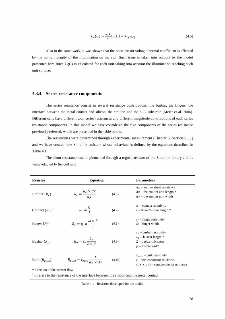
78

(4.5)

Also in the same work, it was shown that the open-circuit voltage thermal coefficient is affected

by the non-uniformity of the illumination on the cell. Such issue is taken into account by the model

presented here since kV(C) is calculated for each unit taking into account the illumination reaching such

unit surface.

4.3.4. Series resistance components

The series resistance consist in several resistance contributions: the busbar, the fingers, the

interface between the metal contact and silicon, the emitter, and the bulk substrate (Meier et al. 2006).

Different cells have different total series resistances and different magnitude contributions of each series

resistance components. In this model we have considered the five components of the series resistance

previously referred, which are presented in the table below.

The resistivities were determined through experimental measurement (Chapter 5, Section 5.1.1)

and we have created new Simulink resistors whose behaviour is defined by the equations described in

Table 4.1.

The shunt resistance was implemented through a regular resistor of the Simulink library and its

value adapted to the cell unit.

Resistor Equation Parameters

Emitter ( )

(4.6)

– emitter sheet resistance

– the emitter unit length *

– the emitter unit width

Contact ( ) 1

(4.7)

– contact resistivity

– finger/busbar length *

Finger ( )

(4.8)

– finger resistivity

– finger width

Busbar ( )

(4.9)

– busbar resistivity

– busbar length *

– busbar thickness

– busbar width

Bulk ( )

(4.10)

– bulk resistivity

– semiconductor thickness

– semiconductor unit area

* direction of the current flow 1 it refers to the resistance of the interface between the silicon and the metal contact.

Table 4.1 - Resistors developed for the model.

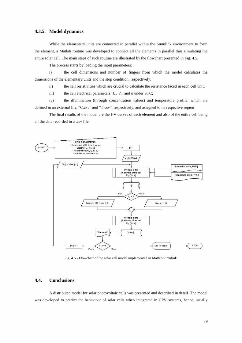
79

4.3.5. Model dynamics

While the elementary units are connected in parallel within the Simulink environment to form

the element, a Matlab routine was developed to connect all the elements in parallel thus simulating the

entire solar cell. The main steps of such routine are illustrated by the flowchart presented in Fig. 4.5.

The process starts by loading the input parameters:

i) the cell dimensions and number of fingers from which the model calculates the

dimensions of the elementary units and the stop condition, respectively;

ii) the cell resistivities which are crucial to calculate the resistance faced in each cell unit;

iii) the cell electrical parameters, Isc, Voc and n under STC;

iv) the illumination (through concentration values) and temperature profile, which are

defined in an external file, “C.csv” and “T.csv”, respectively, and assigned to its respective region

The final results of the model are the I-V curves of each element and also of the entire cell being

all the data recorded in a .csv file.

Fig. 4.5 - Flowchart of the solar cell model implemented in Matlab/Simulink.

4.4. Conclusions

A distributed model for solar photovoltaic cells was presented and described in detail. The model

was developed to predict the behaviour of solar cells when integrated in CPV systems, hence, usually

80

exposed to inhomogeneous illumination and temperature profiles. Without loss of generality, the model

was implemented for a silicon solar cell with laser grooved buried contacts (LGBC).

Model validation will be addressed in Chapter 6, a set of inhomogeneous illumination and

temperature profiles will be modelled and experimentally tested within a temperature range of 25°C up to

70°C and a concentration level from 1 sun up to 30suns.

References

Ánton, I., Sala, G. & Pachón, D., 2001. Correction of the Voc vs. temperature dependence under non-

uniform concentrated illumination. In Proceedings of the 17th European Photovoltaic Solar Energy

Conference. Munich, p. 156.

Chemisana, Daniel & Rosell, J.I., 2011. Electrical performance increase of concentrator solar cells under

Gaussian temperature profiles. Progress in Photovoltaics: Research and Applications. Available at:

http://onlinelibrary.wiley.com/doi/10.1002/pip.1205/full [Accessed January 13, 2012].

Coventry, J S, Franklin, E & Blakers, A., 2004. Thermal and electrical performance of a concentrating

PV / Thermal collector : results from the ANU CHAPS collector,

Coventry, Joe S., 2005. Performance of a concentrating photovoltaic/thermal solar collector. Solar

Energy, 78(2), pp.211–222. Available at:

http://linkinghub.elsevier.com/retrieve/pii/S0038092X04000635 [Accessed April 11, 2012].

Cuevas, A. & López-Romero, S., 1984. The combined effect of non-uniform illumination and series

resistance on the open-circuit voltage of solar cells. Solar Cells, 11, pp.163–173. Available at:

http://linkinghub.elsevier.com/retrieve/pii/0379678784900243.

Domenech-Garret, J.-L., 2011. Cell behaviour under different non-uniform temperature and radiation

combined profiles using a two dimensional finite element model. Solar Energy, 85(2), pp.256–264.

Available at: http://linkinghub.elsevier.com/retrieve/pii/S0038092X10003725 [Accessed March 9,

2013].

Franklin, ET & Coventry, J., 2002. Effects of highly non-uniform illumination distribution on electrical

performance of solar cells. In Proceedings of the 40th Annual Conference for the Australian New

Zealand Solar Energy Society. Available at: http://en.scientificcommons.org/51507296 [Accessed

January 13, 2012].

Garner, C.M. & Nsaby, R.D., 1979. Effects of nonuniform illumination on the performance of silicon

concentrator solar cells. In Tech. Dig. Int. Electron Devices Meet. Washington, D.C.: IEEE, pp.

312–313.

Ghitas, A.E. & Sabry, M., 2006. A study of the effect of shadowing location and area on the Si solar cell

electrical parameters. Vacuum, 81(4), pp.475–478. Available at:

http://linkinghub.elsevier.com/retrieve/pii/S0042207X06002181 [Accessed January 13, 2012].

Luque, A., Sala, G. & Arboiro, J., 1998. Electric and thermal model for non-uniformly illuminated

concentration cells. Solar energy materials and solar cells, 51(3), pp.269–290. Available at:

http://lib.semi.ac.cn:8080/tsh/dzzy/wsqk/selected papers/Solar Energy Materials and Solar Cells/51-

269.pdf [Accessed January 13, 2012].

Matlab, Diode. Available at: http://www.mathworks.com/help/toolbox/physmod/elec/ref/diode.html.

81

Meier, D., Good, E. & Garcia, R., 2006. Determining components of series resistance from measurements

on a finished cell. In Photovoltaic Energy Conversion, Conference Record of the 2006 IEEE 4th

World Conference on. Ieee, pp. 1315–1318. Available at:

http://ieeexplore.ieee.org/lpdocs/epic03/wrapper.htm?arnumber=4059886 [Accessed January 13,

2012].

Mellor, A. et al., 2009. A two-dimensional finite element model of front surface current flow in cells

under non-uniform, concentrated illumination. Solar Energy, 83(9), pp.1459–1465. Available at:

http://linkinghub.elsevier.com/retrieve/pii/S0038092X09000772 [Accessed January 13, 2012].

Mitchell, K.W., 1977. Computer analysis of resistance and non-uniform illumination effects on

concentrator solar cells. In Tech. Dig. Int. Electron Devices Meet. Washington DC: IEEE, pp. 1–4.

Pfeiffer, H. & Bihler, M., 1982. The effects of non-uniform illumination of solar cells with concentrated

light. Solar Cells, 5, pp.293–299.

Rosell, J.I. & Ibáñez, M., 2006. Modelling power output in photovoltaic modules for outdoor operating

conditions. Energy Conversion and Management, 47(15-16), pp.2424–2430. Available at:

http://linkinghub.elsevier.com/retrieve/pii/S0196890405003092 [Accessed February 1, 2012].

Sabry, M. & Ghitas, A.E., 2006. Effect of edge shading on the performance of silicon solar cell. Vacuum,

80(5), pp.444–450. Available at: http://linkinghub.elsevier.com/retrieve/pii/S0042207X05002447

[Accessed January 13, 2012].

Villalva, M.G., Gazoli, J.R. & Filho, E.R., 2009. Modeling and circuit-based simulation of photovoltaic

arrays. 2009 Brazilian Power Electronics Conference, pp.1244–1254. Available at:

http://ieeexplore.ieee.org/lpdocs/epic03/wrapper.htm?arnumber=5347680.

82

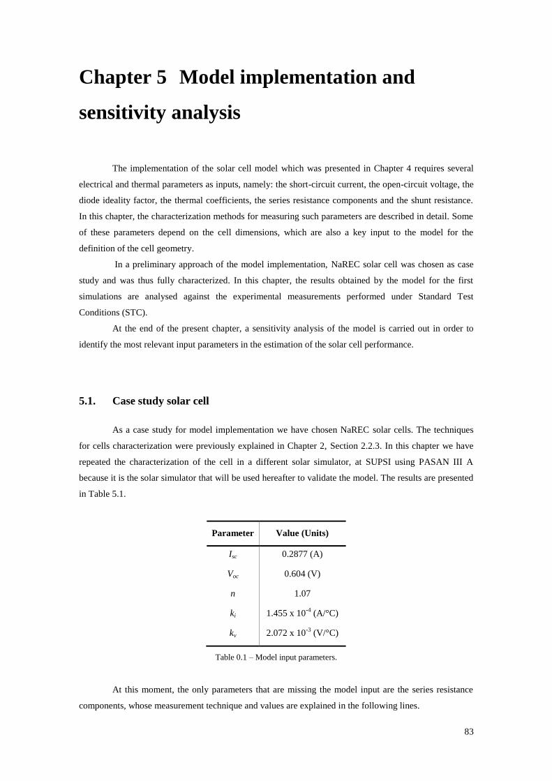
83

Chapter 5 Model implementation and

sensitivity analysis

The implementation of the solar cell model which was presented in Chapter 4 requires several

electrical and thermal parameters as inputs, namely: the short-circuit current, the open-circuit voltage, the

diode ideality factor, the thermal coefficients, the series resistance components and the shunt resistance.

In this chapter, the characterization methods for measuring such parameters are described in detail. Some

of these parameters depend on the cell dimensions, which are also a key input to the model for the

definition of the cell geometry.

In a preliminary approach of the model implementation, NaREC solar cell was chosen as case

study and was thus fully characterized. In this chapter, the results obtained by the model for the first

simulations are analysed against the experimental measurements performed under Standard Test

Conditions (STC).

At the end of the present chapter, a sensitivity analysis of the model is carried out in order to

identify the most relevant input parameters in the estimation of the solar cell performance.

5.1. Case study solar cell

As a case study for model implementation we have chosen NaREC solar cells. The techniques

for cells characterization were previously explained in Chapter 2, Section 2.2.3. In this chapter we have

repeated the characterization of the cell in a different solar simulator, at SUPSI using PASAN III A

because it is the solar simulator that will be used hereafter to validate the model. The results are presented

in Table 5.1.

Parameter Value (Units)

Isc 0.2877 (A)

Voc 0.604 (V)

n 1.07

ki 1.455 x 10-4

(A/°C)

kv 2.072 x 10-3

(V/°C)

Table 0.1 – Model input parameters.

At this moment, the only parameters that are missing the model input are the series resistance

components, whose measurement technique and values are explained in the following lines.

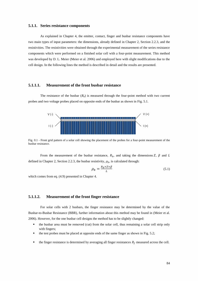
84

5.1.1. Series resistance components

As explained in Chapter 4, the emitter, contact, finger and busbar resistance components have

two main types of input parameters: the dimensions, already defined in Chapter 2, Section 2.2.3, and the

resistivities. The resistivities were obtained through the experimental measurement of the series resistance

components which were performed on a finished solar cell with a four-point measurement. This method

was developed by D. L. Meier (Meier et al. 2006) and employed here with slight modifications due to the

cell design. In the following lines the method is described in detail and the results are presented.

5.1.1.1. Measurement of the front busbar resistance

The resistance of the busbar (Rb) is measured through the four-point method with two current

probes and two voltage probes placed on opposite ends of the busbar as shown in Fig. 5.1.

Fig. 0.1 - Front grid pattern of a solar cell showing the placement of the probes for a four-point measurement of the

busbar resistance.

From the measurement of the busbar resistance, , and taking the dimensions , and

defined in Chapter 2, Section 2.2.3, the busbar resistivity, , is calculated through:

(5.1)

which comes from eq. (4.9) presented in Chapter 4.

5.1.1.2. Measurement of the front finger resistance

For solar cells with 2 busbars, the finger resistance may be determined by the value of the

Busbar-to-Busbar Resistance (BBR), further information about this method may be found in (Meier et al.

2006). However, for the one busbar cell designs the method has to be slightly changed:

the busbar area must be removed (cut) from the solar cell, thus remaining a solar cell strip only

with fingers;

the test probes must be placed at opposite ends of the same finger as shown in Fig. 5.2;

the finger resistance is determined by averaging all finger resistances measured across the cell.

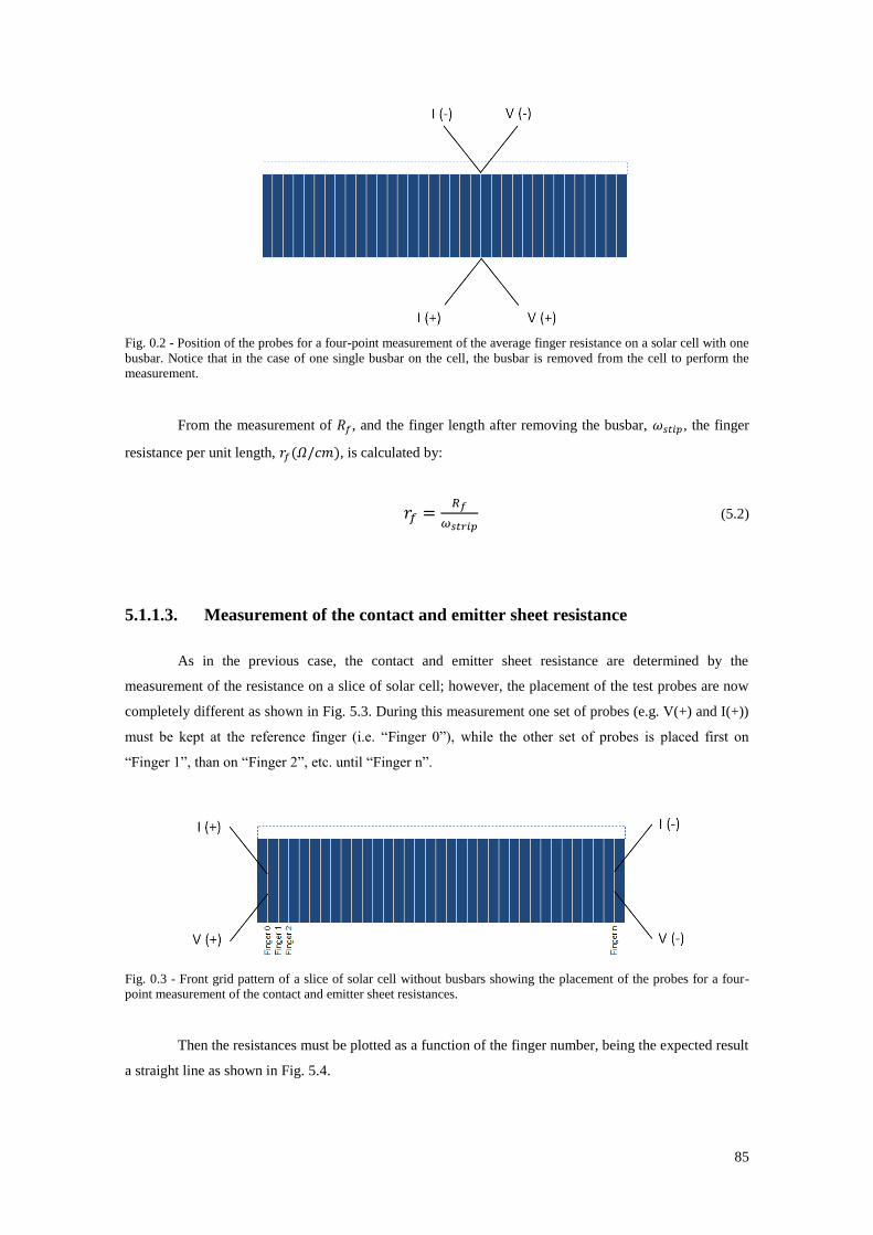
85

Fig. 0.2 - Position of the probes for a four-point measurement of the average finger resistance on a solar cell with one

busbar. Notice that in the case of one single busbar on the cell, the busbar is removed from the cell to perform the

measurement.

From the measurement of , and the finger length after removing the busbar, , the finger

resistance per unit length, , is calculated by:

(5.2)

5.1.1.3. Measurement of the contact and emitter sheet resistance

As in the previous case, the contact and emitter sheet resistance are determined by the

measurement of the resistance on a slice of solar cell; however, the placement of the test probes are now

completely different as shown in Fig. 5.3. During this measurement one set of probes (e.g. V(+) and I(+))

must be kept at the reference finger (i.e. “Finger 0”), while the other set of probes is placed first on

“Finger 1”, than on “Finger 2”, etc. until “Finger n”.

Fig. 0.3 - Front grid pattern of a slice of solar cell without busbars showing the placement of the probes for a four-

point measurement of the contact and emitter sheet resistances.

Then the resistances must be plotted as a function of the finger number, being the expected result

a straight line as shown in Fig. 5.4.

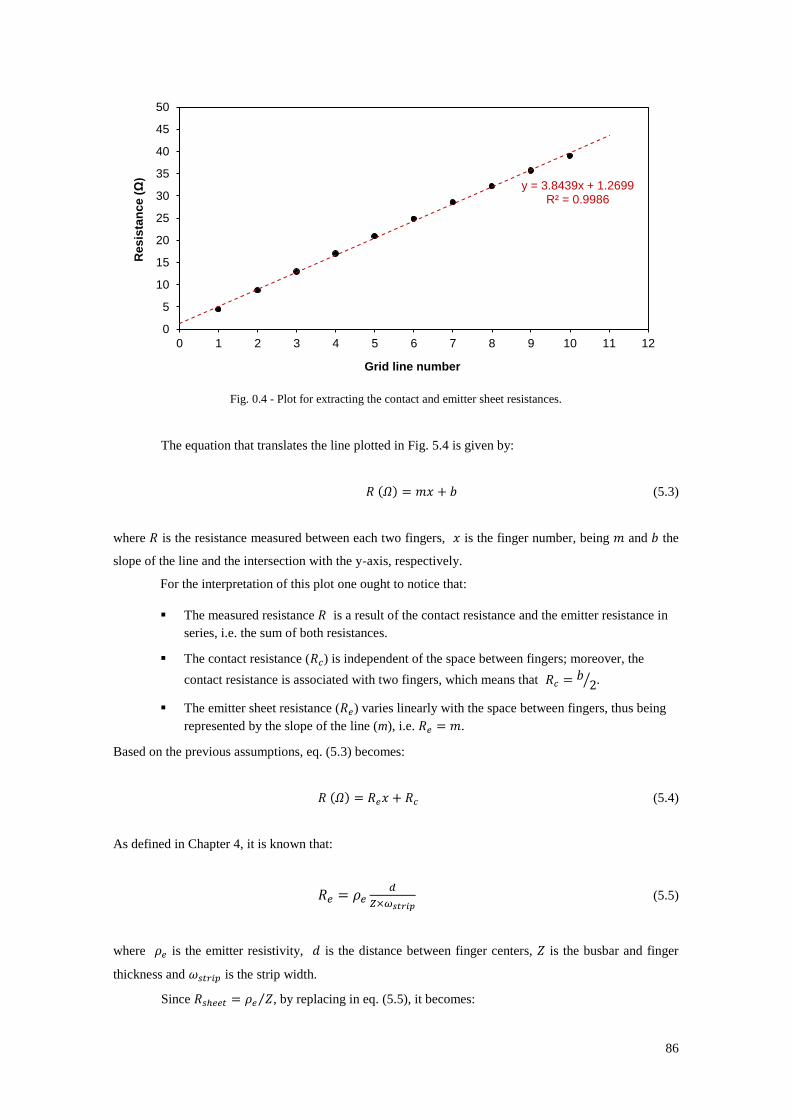
86

Fig. 0.4 - Plot for extracting the contact and emitter sheet resistances.

The equation that translates the line plotted in Fig. 5.4 is given by:

(5.3)

where is the resistance measured between each two fingers, is the finger number, being and the

slope of the line and the intersection with the y-axis, respectively.

For the interpretation of this plot one ought to notice that:

The measured resistance is a result of the contact resistance and the emitter resistance in

series, i.e. the sum of both resistances.

The contact resistance ( ) is independent of the space between fingers; moreover, the

contact resistance is associated with two fingers, which means that ⁄ .

The emitter sheet resistance ( ) varies linearly with the space between fingers, thus being

represented by the slope of the line (m), i.e. .

Based on the previous assumptions, eq. (5.3) becomes:

(5.4)

As defined in Chapter 4, it is known that:

(5.5)

where is the emitter resistivity, is the distance between finger centers, is the busbar and finger

thickness and is the strip width.

Since ⁄ , by replacing in eq. (5.5), it becomes:

y = 3.8439x + 1.2699 R² = 0.9986

0

5

10

15

20

25

30

35

40

45

50

0 1 2 3 4 5 6 7 8 9 10 11 12

Re

sis

tan

ce

(Ω

)

Grid line number

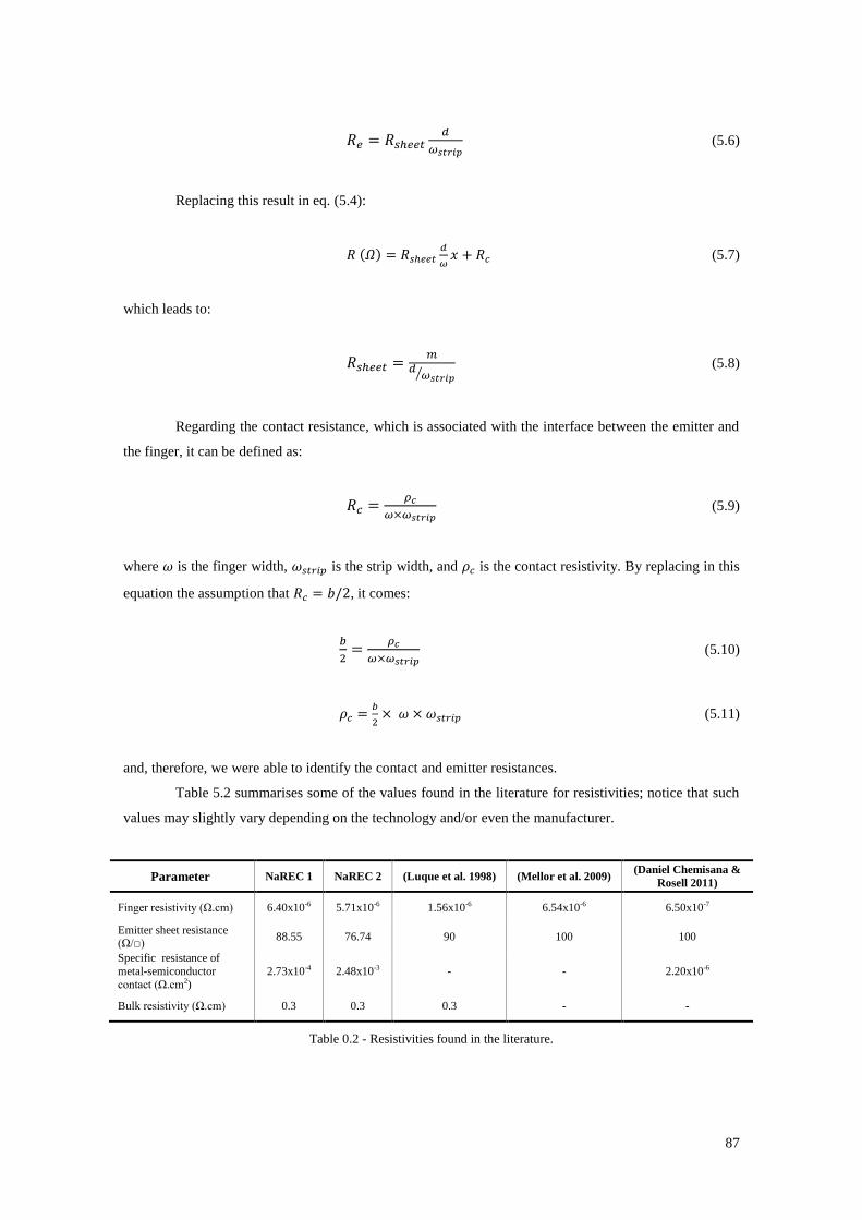
87

(5.6)

Replacing this result in eq. (5.4):

(5.7)

which leads to:

⁄

(5.8)

Regarding the contact resistance, which is associated with the interface between the emitter and

the finger, it can be defined as:

(5.9)

where is the finger width, is the strip width, and is the contact resistivity. By replacing in this

equation the assumption that , it comes:

(5.10)

(5.11)

and, therefore, we were able to identify the contact and emitter resistances.

Table 5.2 summarises some of the values found in the literature for resistivities; notice that such

values may slightly vary depending on the technology and/or even the manufacturer.

Parameter NaREC 1 NaREC 2 (Luque et al. 1998) (Mellor et al. 2009) (Daniel Chemisana &

Rosell 2011)

Finger resistivity (Ω.cm) 6.40x10-6 5.71x10-6 1.56x10-6 6.54x10-6 6.50x10-7

Emitter sheet resistance (Ω/□)

88.55 76.74 90 100 100

Specific resistance of

metal-semiconductor contact (Ω.cm2)

2.73x10-4 2.48x10-3 - - 2.20x10-6

Bulk resistivity (Ω.cm) 0.3 0.3 0.3 - -

Table 0.2 - Resistivities found in the literature.

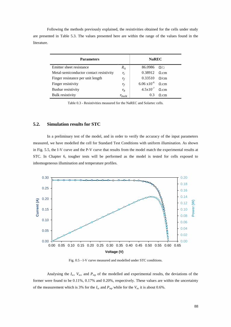
88

Following the methods previously explained, the resistivities obtained for the cells under study

are presented in Table 5.3. The values presented here are within the range of the values found in the

literature.

Parameters NaREC

Emitter sheet resistance 86.0986 Ω/□

Metal-semiconductor contact resistivity 0.38912 Ω.cm

Finger resistance per unit length 0.33510 Ω/cm

Finger resistivity 6.06 x10-6

Ω.cm

Busbar resistivity 4.5x10-7

Ω.cm

Bulk resistivity 0.3 Ω.cm

Table 0.3 - Resistivities measured for the NaREC and Solartec cells.

5.2. Simulation results for STC

In a preliminary test of the model, and in order to verify the accuracy of the input parameters

measured, we have modelled the cell for Standard Test Conditions with uniform illumination. As shown

in Fig. 5.5, the I-V curve and the P-V curve that results from the model match the experimental results at

STC. In Chapter 6, tougher tests will be performed as the model is tested for cells exposed to

inhomogeneous illumination and temperature profiles.

Fig. 0.5 - I-V curve measured and modelled under STC conditions.

Analysing the Isc, Voc, and Pmp of the modelled and experimental results, the deviations of the

former were found to be 0.11%, 0.17% and 0.20%, respectively. These values are within the uncertainty

of the measurement which is 3% for the Isc and Pmp while for the Voc it is about 0.6%.

0.00

0.02

0.04

0.06

0.08

0.10

0.12

0.14

0.16

0.18

0.20

0.00

0.05

0.10

0.15

0.20

0.25

0.30

0.00 0.05 0.10 0.15 0.20 0.25 0.30 0.35 0.40 0.45 0.50 0.55 0.60 0.65

Po

we

r (W

)

Cu

rre

nt

(A)

Voltage (V)

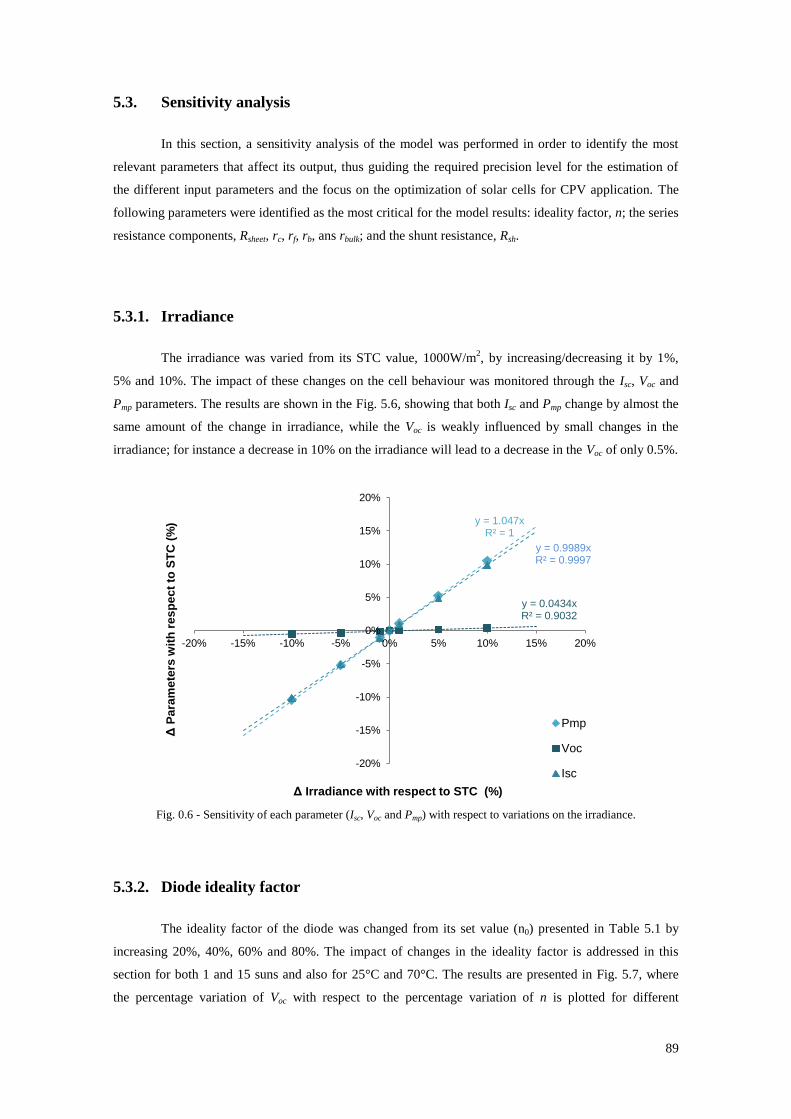
89

5.3. Sensitivity analysis

In this section, a sensitivity analysis of the model was performed in order to identify the most

relevant parameters that affect its output, thus guiding the required precision level for the estimation of

the different input parameters and the focus on the optimization of solar cells for CPV application. The

following parameters were identified as the most critical for the model results: ideality factor, n; the series

resistance components, Rsheet, rc, rf, rb, ans rbulk; and the shunt resistance, Rsh.

5.3.1. Irradiance

The irradiance was varied from its STC value, 1000W/m2, by increasing/decreasing it by 1%,

5% and 10%. The impact of these changes on the cell behaviour was monitored through the Isc, Voc and

Pmp parameters. The results are shown in the Fig. 5.6, showing that both Isc and Pmp change by almost the

same amount of the change in irradiance, while the Voc is weakly influenced by small changes in the

irradiance; for instance a decrease in 10% on the irradiance will lead to a decrease in the Voc of only 0.5%.

Fig. 0.6 - Sensitivity of each parameter (Isc, Voc and Pmp) with respect to variations on the irradiance.

5.3.2. Diode ideality factor

The ideality factor of the diode was changed from its set value (n0) presented in Table 5.1 by

increasing 20%, 40%, 60% and 80%. The impact of changes in the ideality factor is addressed in this

section for both 1 and 15 suns and also for 25°C and 70°C. The results are presented in Fig. 5.7, where

the percentage variation of Voc with respect to the percentage variation of n is plotted for different

y = 1.047x R² = 1

y = 0.0434x R² = 0.9032

y = 0.9989x R² = 0.9997

-20%

-15%

-10%

-5%

0%

5%

10%

15%

20%

-20% -15% -10% -5% 0% 5% 10% 15% 20%

Δ P

ara

me

ters

wit

h r

es

pe

ct

to S

TC

(%

)

Δ Irradiance with respect to STC (%)

Pmp

Voc

Isc

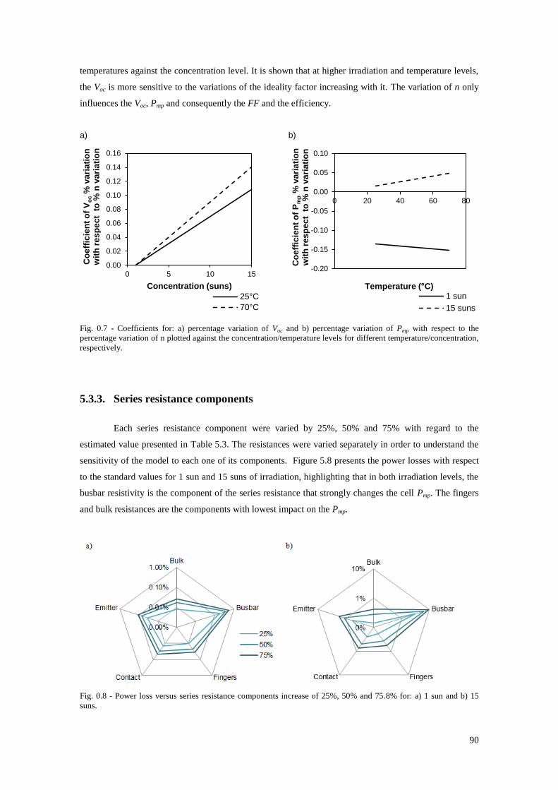
90

temperatures against the concentration level. It is shown that at higher irradiation and temperature levels,

the Voc is more sensitive to the variations of the ideality factor increasing with it. The variation of n only

influences the Voc, Pmp and consequently the FF and the efficiency.

a) b)

Fig. 0.7 - Coefficients for: a) percentage variation of Voc and b) percentage variation of Pmp with respect to the

percentage variation of n plotted against the concentration/temperature levels for different temperature/concentration,

respectively.

5.3.3. Series resistance components

Each series resistance component were varied by 25%, 50% and 75% with regard to the

estimated value presented in Table 5.3. The resistances were varied separately in order to understand the

sensitivity of the model to each one of its components. Figure 5.8 presents the power losses with respect

to the standard values for 1 sun and 15 suns of irradiation, highlighting that in both irradiation levels, the

busbar resistivity is the component of the series resistance that strongly changes the cell Pmp. The fingers

and bulk resistances are the components with lowest impact on the Pmp.

Fig. 0.8 - Power loss versus series resistance components increase of 25%, 50% and 75.8% for: a) 1 sun and b) 15

suns.

0.00

0.02

0.04

0.06

0.08

0.10

0.12

0.14

0.16

0 5 10 15

Co

eff

icie

nt

of

Vo

c %

va

ria

tio

n

wit

h r

es

pe

ct

to

% n

va

ria

tio

n

Concentration (suns)

25°C

70°C

-0.20

-0.15

-0.10

-0.05

0.00

0.05

0.10

0 20 40 60 80

Co

eff

icie

nt

of

Pm

p %

va

ria

tio

n

wit

h r

es

pe

ct

to

% n

va

ria

tio

n

Temperature (°C) 1 sun

15 suns

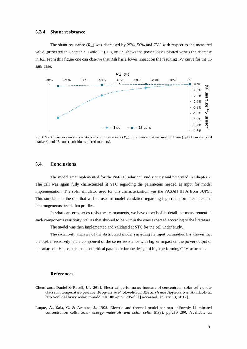
91

5.3.4. Shunt resistance

The shunt resistance (Rsh) was decreased by 25%, 50% and 75% with respect to the measured

value (presented in Chapter 2, Table 2.3). Figure 5.9 shows the power losses plotted versus the decrease

in Rsh. From this figure one can observe that Rsh has a lower impact on the resulting I-V curve for the 15

suns case.

Fig. 0.9 - Power loss versus variation in shunt resistance (Rsh) for a concentration level of 1 sun (light blue diamond

markers) and 15 suns (dark blue squared markers).

5.4. Conclusions

The model was implemented for the NaREC solar cell under study and presented in Chapter 2.

The cell was again fully characterized at STC regarding the parameters needed as input for model

implementation. The solar simulator used for this characterization was the PASAN III A from SUPSI.

This simulator is the one that will be used in model validation regarding high radiation intensities and

inhomogeneous irradiation profiles.

In what concerns series resistance components, we have described in detail the measurement of

each components resistivity, values that showed to be within the ones expected according to the literature.

The model was then implemented and validated at STC for the cell under study.

The sensitivity analysis of the distributed model regarding its input parameters has shown that

the busbar resistivity is the component of the series resistance with higher impact on the power output of

the solar cell. Hence, it is the most critical parameter for the design of high performing CPV solar cells.

References

Chemisana, Daniel & Rosell, J.I., 2011. Electrical performance increase of concentrator solar cells under

Gaussian temperature profiles. Progress in Photovoltaics: Research and Applications. Available at:

http://onlinelibrary.wiley.com/doi/10.1002/pip.1205/full [Accessed January 13, 2012].

Luque, A., Sala, G. & Arboiro, J., 1998. Electric and thermal model for non-uniformly illuminated

concentration cells. Solar energy materials and solar cells, 51(3), pp.269–290. Available at:

-1.6%

-1.4%

-1.2%

-1.0%

-0.8%

-0.6%

-0.4%

-0.2%

0.0%

-80% -70% -60% -50% -40% -30% -20% -10% 0%

Lo

ss

in

Pm

p f

or

1 s

un

(%

)

Rsh (%)

1 sun 15 suns

92

http://lib.semi.ac.cn:8080/tsh/dzzy/wsqk/selected papers/Solar Energy Materials and Solar Cells/51-

269.pdf [Accessed January 13, 2012].

Meier, D., Good, E. & Garcia, R., 2006. Determining components of series resistance from measurements

on a finished cell. In Photovoltaic Energy Conversion, Conference Record of the 2006 IEEE 4th

World Conference on. Ieee, pp. 1315–1318. Available at:

http://ieeexplore.ieee.org/lpdocs/epic03/wrapper.htm?arnumber=4059886 [Accessed January 13,

2012].

Mellor, A. et al., 2009. A two-dimensional finite element model of front surface current flow in cells

under non-uniform, concentrated illumination. Solar Energy, 83(9), pp.1459–1465. Available at:

http://linkinghub.elsevier.com/retrieve/pii/S0038092X09000772 [Accessed January 13, 2012].

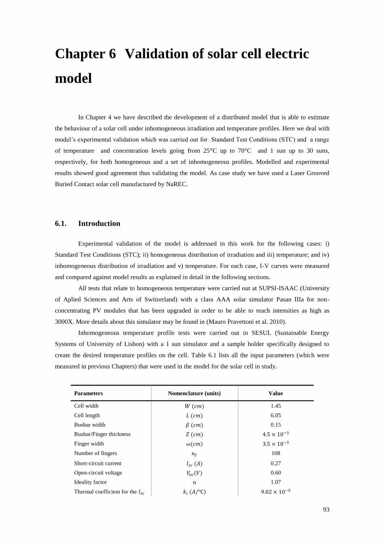
93

Chapter 6 Validation of solar cell electric

model

In Chapter 4 we have described the development of a distributed model that is able to estimate

the behaviour of a solar cell under inhomogeneous irradiation and temperature profiles. Here we deal with

model’s experimental validation which was carried out for Standard Test Conditions (STC) and a range

of temperature and concentration levels going from 25°C up to 70°C and 1 sun up to 30 suns,

respectively, for both homogeneous and a set of inhomogeneous profiles. Modelled and experimental

results showed good agreement thus validating the model. As case study we have used a Laser Grooved

Buried Contact solar cell manufactured by NaREC.

6.1. Introduction

Experimental validation of the model is addressed in this work for the following cases: i)

Standard Test Conditions (STC); ii) homogeneous distribution of irradiation and iii) temperature; and iv)

inhomogeneous distribution of irradiation and v) temperature. For each case, I-V curves were measured

and compared against model results as explained in detail in the following sections.

All tests that relate to homogeneous temperature were carried out at SUPSI-ISAAC (University

of Aplied Sciences and Arts of Switzerland) with a class AAA solar simulator Pasan IIIa for non-

concentrating PV modules that has been upgraded in order to be able to reach intensities as high as

3000X. More details about this simulator may be found in (Mauro Pravettoni et al. 2010).

Inhomogeneous temperature profile tests were carried out in SESUL (Sustainable Energy

Systems of University of Lisbon) with a 1 sun simulator and a sample holder specifically designed to

create the desired temperature profiles on the cell. Table 6.1 lists all the input parameters (which were

measured in previous Chapters) that were used in the model for the solar cell in study.

Parameters Nomenclature (units) Value

Cell width 1.45

Cell length 6.05

Busbar width 0.15

Busbar/Finger thickness

Finger width

Number of fingers 108

Short-circuit current 0.27

Open-circuit voltage 0.60

Ideality factor 1.07

Thermal coefficient for the

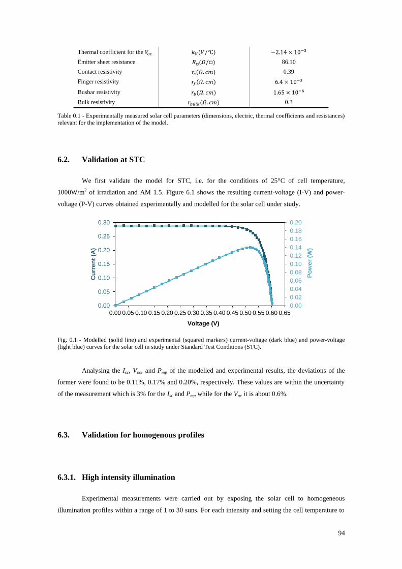
94

Thermal coefficient for the

Emitter sheet resistance 86.10

Contact resistivity 0.39

Finger resistivity

Busbar resistivity

Bulk resistivity 0.3

Table 0.1 - Experimentally measured solar cell parameters (dimensions, electric, thermal coefficients and resistances)

relevant for the implementation of the model.

6.2. Validation at STC

We first validate the model for STC, i.e. for the conditions of 25°C of cell temperature,

1000W/m2 of irradiation and AM 1.5. Figure 6.1 shows the resulting current-voltage (I-V) and power-

voltage (P-V) curves obtained experimentally and modelled for the solar cell under study.

Fig. 0.1 - Modelled (solid line) and experimental (squared markers) current-voltage (dark blue) and power-voltage

(light blue) curves for the solar cell in study under Standard Test Conditions (STC).

Analysing the Isc, Voc, and Pmp of the modelled and experimental results, the deviations of the

former were found to be 0.11%, 0.17% and 0.20%, respectively. These values are within the uncertainty

of the measurement which is 3% for the Isc and Pmp while for the Voc it is about 0.6%.

6.3. Validation for homogenous profiles

6.3.1. High intensity illumination

Experimental measurements were carried out by exposing the solar cell to homogeneous

illumination profiles within a range of 1 to 30 suns. For each intensity and setting the cell temperature to

0.00

0.02

0.04

0.06

0.08

0.10

0.12

0.14

0.16

0.18

0.20

0.00

0.05

0.10

0.15

0.20

0.25

0.30

0.00 0.05 0.10 0.15 0.20 0.25 0.30 0.35 0.40 0.45 0.50 0.55 0.60 0.65P

ow

er

(W)

Cu

rre

nt

(A)

Voltage (V)

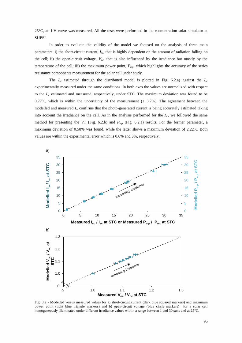
95

25°C, an I-V curve was measured. All the tests were performed in the concentration solar simulator at

SUPSI.

In order to evaluate the validity of the model we focused on the analysis of three main

parameters: i) the short-circuit current, Isc, that is highly dependent on the amount of radiation falling on

the cell; ii) the open-circuit voltage, Voc, that is also influenced by the irradiance but mostly by the

temperature of the cell; iii) the maximum power point, Pmp, which highlights the accuracy of the series

resistance components measurement for the solar cell under study.

The Isc estimated through the distributed model is plotted in Fig. 6.2.a) against the Isc

experimentally measured under the same conditions. In both axes the values are normalized with respect

to the Isc estimated and measured, respectively, under STC. The maximum deviation was found to be

0.77%, which is within the uncertainty of the measurement (± 3.7%). The agreement between the

modelled and measured Isc confirms that the photo-generated current is being accurately estimated taking

into account the irradiance on the cell. As in the analysis performed for the Isc, we followed the same

method for presenting the Voc (Fig. 6.2.b) and Pmp (Fig. 6.2.a) results. For the former parameter, a

maximum deviation of 0.58% was found, while the latter shows a maximum deviation of 2.22%. Both

values are within the experimental error which is 0.6% and 3%, respectively.

a)

b)

Fig. 0.2 - Modelled versus measured values for a) short-circuit current (dark blue squared markers) and maximum

power point (light blue triangle markers) and b) open-circuit voltage (blue circle markers) for a solar cell

homogeneously illuminated under different irradiance values within a range between 1 and 30 suns and at 25°C.

0

5

10

15

20

25

30

35

0

5

10

15

20

25

30

35

0 5 10 15 20 25 30 35

Mo

delled

Pm

p / P

mp a

t S

TC

Mo

delled

Isc/

I sc a

t S

TC

Measured Isc / Isc at STC or Measured Pmp / Pmp at STC

0.9

1.0

1.1

1.2

1.3

0.9 1.0 1.1 1.2 1.3

Mo

delled

Vo

c /

Vo

c a

t S

TC

Measured Voc / Voc at STC

0

0

//

//

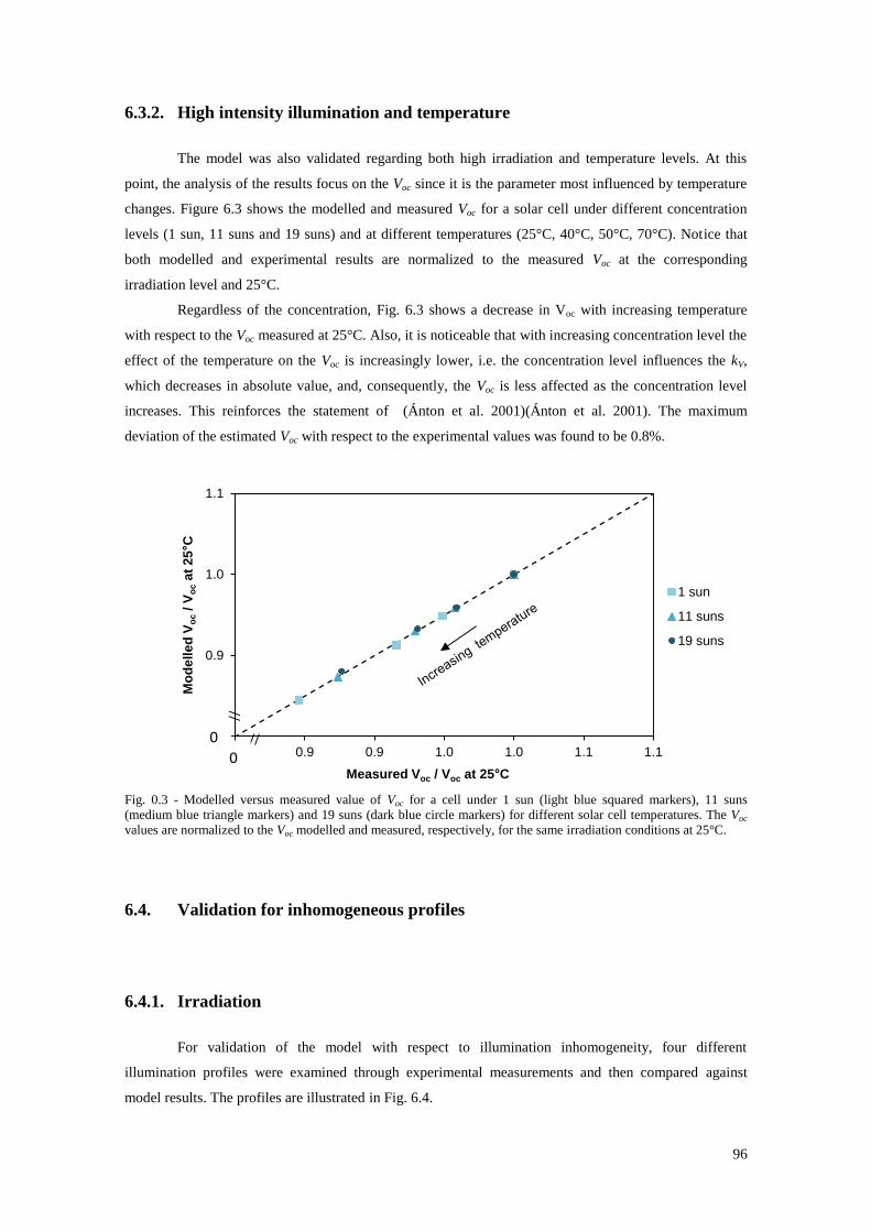
96

6.3.2. High intensity illumination and temperature

The model was also validated regarding both high irradiation and temperature levels. At this

point, the analysis of the results focus on the Voc since it is the parameter most influenced by temperature

changes. Figure 6.3 shows the modelled and measured Voc for a solar cell under different concentration

levels (1 sun, 11 suns and 19 suns) and at different temperatures (25°C, 40°C, 50°C, 70°C). Notice that

both modelled and experimental results are normalized to the measured Voc at the corresponding

irradiation level and 25°C.

Regardless of the concentration, Fig. 6.3 shows a decrease in Voc with increasing temperature

with respect to the Voc measured at 25°C. Also, it is noticeable that with increasing concentration level the

effect of the temperature on the Voc is increasingly lower, i.e. the concentration level influences the kV,

which decreases in absolute value, and, consequently, the Voc is less affected as the concentration level

increases. This reinforces the statement of (Ánton et al. 2001)(Ánton et al. 2001). The maximum

deviation of the estimated Voc with respect to the experimental values was found to be 0.8%.

Fig. 0.3 - Modelled versus measured value of Voc for a cell under 1 sun (light blue squared markers), 11 suns

(medium blue triangle markers) and 19 suns (dark blue circle markers) for different solar cell temperatures. The Voc

values are normalized to the Voc modelled and measured, respectively, for the same irradiation conditions at 25°C.

6.4. Validation for inhomogeneous profiles

6.4.1. Irradiation

For validation of the model with respect to illumination inhomogeneity, four different

illumination profiles were examined through experimental measurements and then compared against

model results. The profiles are illustrated in Fig. 6.4.

0.8

0.9

1.0

1.1

0.8 0.9 0.9 1.0 1.0 1.1 1.1

Mo

de

lle

d V

oc / V

oc a

t 2

5°C

Measured Voc / Voc at 25°C

1 sun

11 suns

19 suns

//

//

0

0

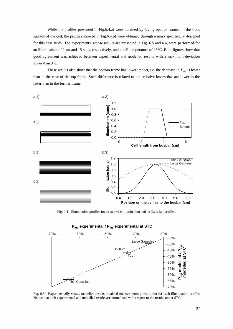
97

While the profiles presented in Fig.6.4.a) were obtained by laying opaque frames on the front

surface of the cell, the profiles showed in Fig.6.4.b) were obtained through a mask specifically designed

for this case study. The experiments, whose results are presented in Fig. 6.5 and 6.6, were performed for

an illumination of 1sun and 15 suns, respectively, and a cell temperature of 25°C. Both figures show that

good agreement was achieved between experimental and modelled results with a maximum deviation

lower than 3%.

These results also show that the bottom frame has lower impact, i.e. the decrease in Pmp is lower

than in the case of the top frame. Such difference is related to the resistive losses that are lower in the

latter than in the former frame.

a.1) a.3)

a.2)

b.1) b.3)

b.2)

Fig. 0.4 - Illumination profiles for a) stepwise illumination and b) Gaussian profiles.

Fig. 0.5 - Experimentally versus modelled results obtained for maximum power point for each illumination profile.

Notice that both experimental and modelled results are normalized with respect to the results under STC.

0.0

0.2

0.4

0.6

0.8

1.0

1.2

0 2 4 6

Illu

min

ati

on

(s

un

s)

Cell length from busbar (cm)

Top

Bottom

0.0

0.2

0.4

0.6

0.8

1.0

1.2

0.0 1.0 2.0 3.0 4.0 5.0 6.0

Illu

min

ati

on

(s

un

s)

Position on the cell as to the busbar (cm)

Thin GaussianLarge Gaussian

Bottom

Top

Thin Gaussian

Large Gaussian

-70%

-65%

-60%

-55%

-50%

-45%

-40%

-35%

-30%

-70% -60% -50% -40% -30%

Pm

p m

od

elled

/ P

mp

mo

delled

at

ST

C

Pmp experimental / Pmp experimental at STC

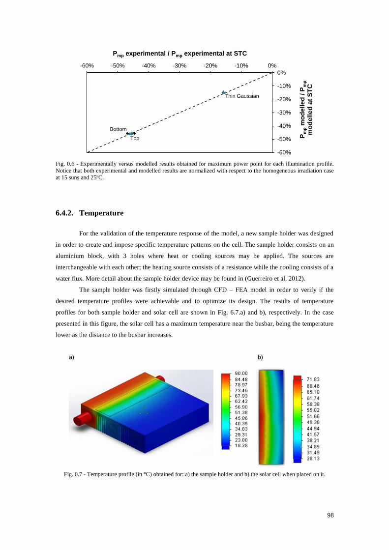
98

Fig. 0.6 - Experimentally versus modelled results obtained for maximum power point for each illumination profile.

Notice that both experimental and modelled results are normalized with respect to the homogeneous irradiation case

at 15 suns and 25ºC.

6.4.2. Temperature

For the validation of the temperature response of the model, a new sample holder was designed

in order to create and impose specific temperature patterns on the cell. The sample holder consists on an

aluminium block, with 3 holes where heat or cooling sources may be applied. The sources are

interchangeable with each other; the heating source consists of a resistance while the cooling consists of a

water flux. More detail about the sample holder device may be found in (Guerreiro et al. 2012).

The sample holder was firstly simulated through CFD – FEA model in order to verify if the

desired temperature profiles were achievable and to optimize its design. The results of temperature

profiles for both sample holder and solar cell are shown in Fig. 6.7.a) and b), respectively. In the case

presented in this figure, the solar cell has a maximum temperature near the busbar, being the temperature

lower as the distance to the busbar increases.

a) b)

Fig. 0.7 - Temperature profile (in °C) obtained for: a) the sample holder and b) the solar cell when placed on it.

Bottom

Top

Thin Gaussian

-60%

-50%

-40%

-30%

-20%

-10%

0%

-60% -50% -40% -30% -20% -10% 0%

Pm

p m

od

elled

/ P

mp

mo

delled

at

ST

C

Pmp experimental / Pmp experimental at STC

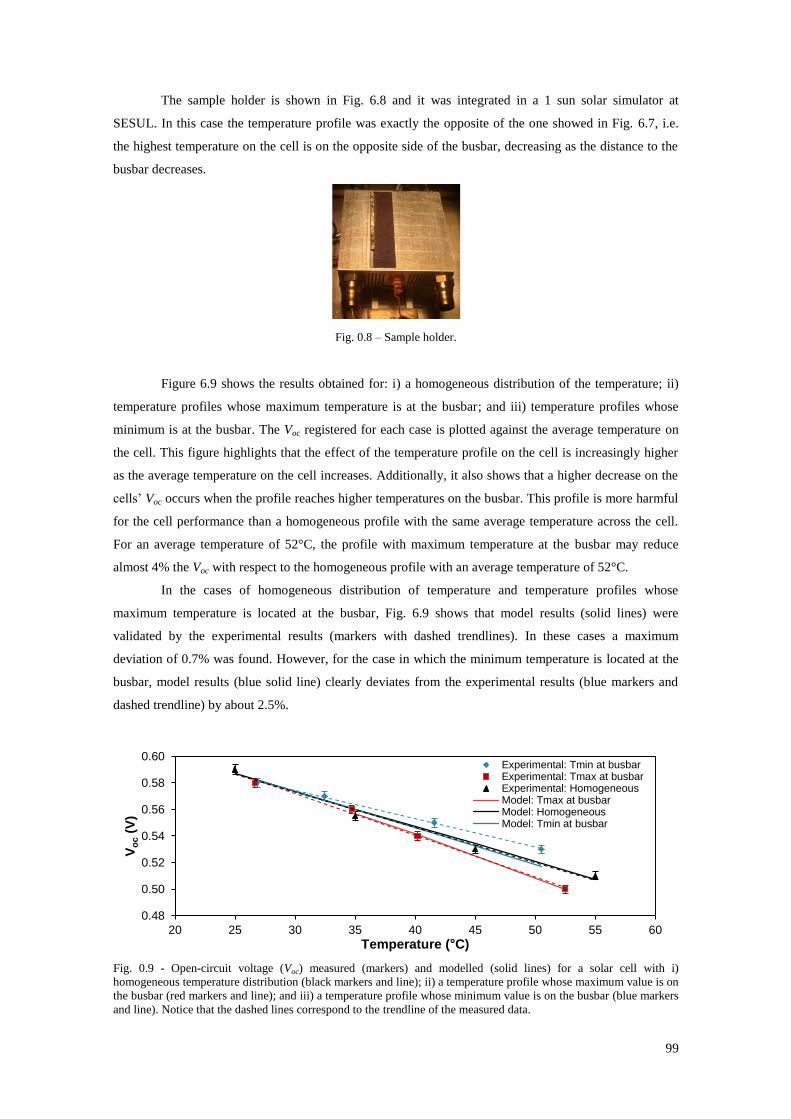
99

The sample holder is shown in Fig. 6.8 and it was integrated in a 1 sun solar simulator at

SESUL. In this case the temperature profile was exactly the opposite of the one showed in Fig. 6.7, i.e.

the highest temperature on the cell is on the opposite side of the busbar, decreasing as the distance to the

busbar decreases.

Fig. 0.8 – Sample holder.

Figure 6.9 shows the results obtained for: i) a homogeneous distribution of the temperature; ii)

temperature profiles whose maximum temperature is at the busbar; and iii) temperature profiles whose

minimum is at the busbar. The Voc registered for each case is plotted against the average temperature on

the cell. This figure highlights that the effect of the temperature profile on the cell is increasingly higher

as the average temperature on the cell increases. Additionally, it also shows that a higher decrease on the

cells’ Voc occurs when the profile reaches higher temperatures on the busbar. This profile is more harmful

for the cell performance than a homogeneous profile with the same average temperature across the cell.

For an average temperature of 52°C, the profile with maximum temperature at the busbar may reduce

almost 4% the Voc with respect to the homogeneous profile with an average temperature of 52°C.

In the cases of homogeneous distribution of temperature and temperature profiles whose

maximum temperature is located at the busbar, Fig. 6.9 shows that model results (solid lines) were

validated by the experimental results (markers with dashed trendlines). In these cases a maximum

deviation of 0.7% was found. However, for the case in which the minimum temperature is located at the

busbar, model results (blue solid line) clearly deviates from the experimental results (blue markers and

dashed trendline) by about 2.5%.

Fig. 0.9 - Open-circuit voltage (Voc) measured (markers) and modelled (solid lines) for a solar cell with i)

homogeneous temperature distribution (black markers and line); ii) a temperature profile whose maximum value is on

the busbar (red markers and line); and iii) a temperature profile whose minimum value is on the busbar (blue markers

and line). Notice that the dashed lines correspond to the trendline of the measured data.

0.48

0.50

0.52

0.54

0.56

0.58

0.60

20 25 30 35 40 45 50 55 60

Vo

c (

V)

Temperature (°C)

Experimental: Tmin at busbarExperimental: Tmax at busbarExperimental: HomogeneousModel: Tmax at busbarModel: HomogeneousModel: Tmin at busbar

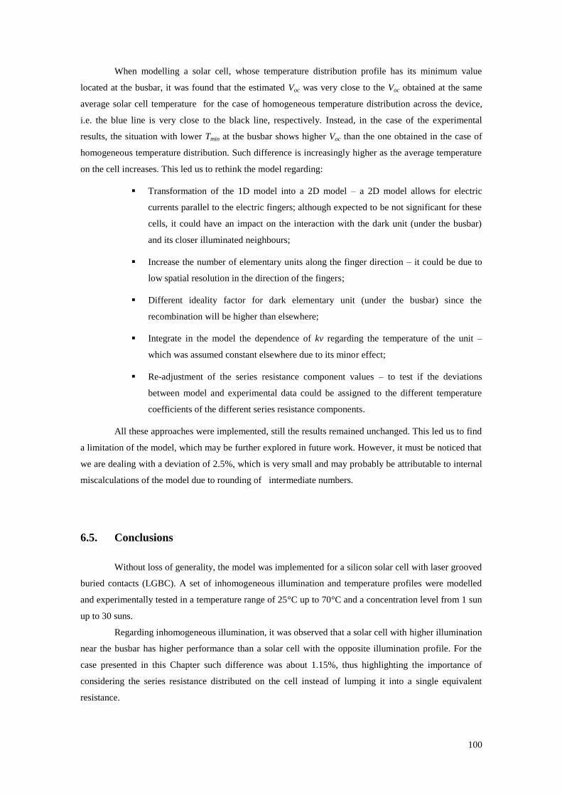
100

When modelling a solar cell, whose temperature distribution profile has its minimum value

located at the busbar, it was found that the estimated Voc was very close to the Voc obtained at the same

average solar cell temperature for the case of homogeneous temperature distribution across the device,

i.e. the blue line is very close to the black line, respectively. Instead, in the case of the experimental

results, the situation with lower Tmin at the busbar shows higher Voc than the one obtained in the case of

homogeneous temperature distribution. Such difference is increasingly higher as the average temperature

on the cell increases. This led us to rethink the model regarding:

Transformation of the 1D model into a 2D model – a 2D model allows for electric

currents parallel to the electric fingers; although expected to be not significant for these

cells, it could have an impact on the interaction with the dark unit (under the busbar)

and its closer illuminated neighbours;

Increase the number of elementary units along the finger direction – it could be due to

low spatial resolution in the direction of the fingers;

Different ideality factor for dark elementary unit (under the busbar) since the

recombination will be higher than elsewhere;

Integrate in the model the dependence of kv regarding the temperature of the unit –

which was assumed constant elsewhere due to its minor effect;

Re-adjustment of the series resistance component values – to test if the deviations

between model and experimental data could be assigned to the different temperature

coefficients of the different series resistance components.

All these approaches were implemented, still the results remained unchanged. This led us to find

a limitation of the model, which may be further explored in future work. However, it must be noticed that

we are dealing with a deviation of 2.5%, which is very small and may probably be attributable to internal

miscalculations of the model due to rounding of intermediate numbers.

6.5. Conclusions

Without loss of generality, the model was implemented for a silicon solar cell with laser grooved

buried contacts (LGBC). A set of inhomogeneous illumination and temperature profiles were modelled

and experimentally tested in a temperature range of 25°C up to 70°C and a concentration level from 1 sun

up to 30 suns.

Regarding inhomogeneous illumination, it was observed that a solar cell with higher illumination

near the busbar has higher performance than a solar cell with the opposite illumination profile. For the

case presented in this Chapter such difference was about 1.15%, thus highlighting the importance of

considering the series resistance distributed on the cell instead of lumping it into a single equivalent

resistance.

101

When comparing homogeneous temperature profiles against temperature profiles whose

maximum temperature is near the busbar, the case study presented here showed that, for the same average

temperature of 52°C, the latter may decrease the Voc in about 4%. It was also showed that with increasing

average temperature the difference between the effect on Voc due to a homogeneous temperature profile

and due to an inhomogeneous profile is increasingly higher.

This Chapter highlighted the importance of using distributed models for solar cells when

predicting their behaviour under conditions of inhomogeneous distribution of temperature and

illumination. The effect of such inhomogeneous profiles, the model’s sensitivity and comparison with

standard model results are further explored in the next Chapter and in (Reis et al. 2013).

References

Ánton, I., Sala, G. & Pachón, D., 2001. Correction of the Voc vs. temperature dependence under non-

uniform concentrated illumination. In Proceedings of the 17th European Photovoltaic Solar Energy

Conference. Munich, p. 156.

Guerreiro, C., Batista, F. & Pimentel, T., 2012. Projecto Final de Licenciatura: Estudo da influência do

perfil de temperatura de uma célula fotovoltaica no seu desempenho eléctrico. Faculdade de

Ciências, Universidade de Lisboa.

Pravettoni, Mauro et al., 2010. Characterization of a pulsed solar simulator for concentrator photovoltaic

cell calibration. Measurement Science and Technology, 21(11), p.115901. Available at:

http://stacks.iop.org/0957-

0233/21/i=11/a=115901?key=crossref.fb808adffcf1b32f18979ae2a69189f2 [Accessed March 26,

2013].

Reis, F. et al., 2013. Exploring the effects of inhomogeneous irradiation and temperature profiles on CPV

solar cells behaviour. Paper submitted to IEEE Journal of Photovoltaics.

102

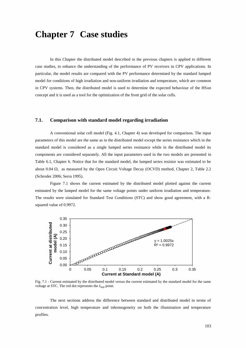
103

Chapter 7 Case studies

In this Chapter the distributed model described in the previous chapters is applied to different

case studies, to enhance the understanding of the performance of PV receivers in CPV applications. In

particular, the model results are compared with the PV performance determined by the standard lumped

model for conditions of high irradiation and non-uniform irradiation and temperature, which are common

in CPV systems. Then, the distributed model is used to determine the expected behaviour of the HSun

concept and it is used as a tool for the optimization of the front grid of the solar cells.

7.1. Comparison with standard model regarding irradiation

A conventional solar cell model (Fig. 4.1, Chapter 4) was developed for comparison. The input

parameters of this model are the same as in the distributed model except the series resistance which in the

standard model is considered as a single lumped series resistance while in the distributed model its

components are considered separately. All the input parameters used in the two models are presented in

Table 6.1, Chapter 6. Notice that for the standard model, the lumped series resistor was estimated to be

about 0.04 , as measured by the Open Circuit Voltage Decay (OCVD) method, Chapter 2, Table 2.2

(Schroder 2006; Serra 1995).

Figure 7.1 shows the current estimated by the distributed model plotted against the current

estimated by the lumped model for the same voltage points under uniform irradiation and temperature.

The results were simulated for Standard Test Conditions (STC) and show good agreement, with a R-

squared value of 0.9972.

Fig. 7.1 - Current estimated by the distributed model versus the current estimated by the standard model for the same

voltage at STC. The red dot represents the Impp point.

The next sections address the difference between standard and distributed model in terms of

concentration level, high temperature and inhomogeneity on both the illumination and temperature

profiles.

y = 1.0025x R² = 0.9972

0.00

0.05

0.10

0.15

0.20

0.25

0.30

0.35

0 0.05 0.1 0.15 0.2 0.25 0.3 0.35

Cu

rren

t at

dis

trib

ute

d

mo

del

(A)

Current at Standard model (A)

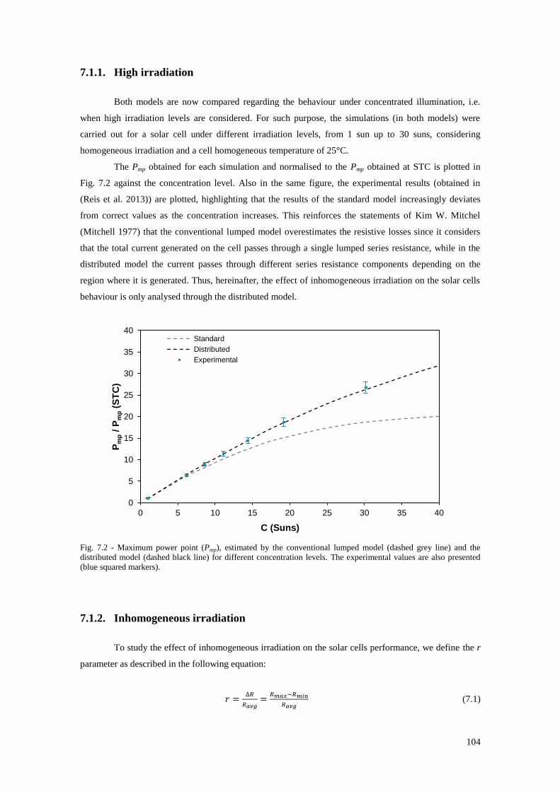
104

7.1.1. High irradiation

Both models are now compared regarding the behaviour under concentrated illumination, i.e.

when high irradiation levels are considered. For such purpose, the simulations (in both models) were

carried out for a solar cell under different irradiation levels, from 1 sun up to 30 suns, considering

homogeneous irradiation and a cell homogeneous temperature of 25°C.

The Pmp obtained for each simulation and normalised to the Pmp obtained at STC is plotted in

Fig. 7.2 against the concentration level. Also in the same figure, the experimental results (obtained in

(Reis et al. 2013)) are plotted, highlighting that the results of the standard model increasingly deviates

from correct values as the concentration increases. This reinforces the statements of Kim W. Mitchel

(Mitchell 1977) that the conventional lumped model overestimates the resistive losses since it considers

that the total current generated on the cell passes through a single lumped series resistance, while in the

distributed model the current passes through different series resistance components depending on the

region where it is generated. Thus, hereinafter, the effect of inhomogeneous irradiation on the solar cells

behaviour is only analysed through the distributed model.

Fig. 7.2 - Maximum power point (Pmp), estimated by the conventional lumped model (dashed grey line) and the

distributed model (dashed black line) for different concentration levels. The experimental values are also presented

(blue squared markers).

7.1.2. Inhomogeneous irradiation

To study the effect of inhomogeneous irradiation on the solar cells performance, we define the r

parameter as described in the following equation:

(7.1)

0

5

10

15

20

25

30

35

40

0 5 10 15 20 25 30 35 40

Pm

p / P

mp (

ST

C)

C (Suns)

Standard

Distributed

Experimental

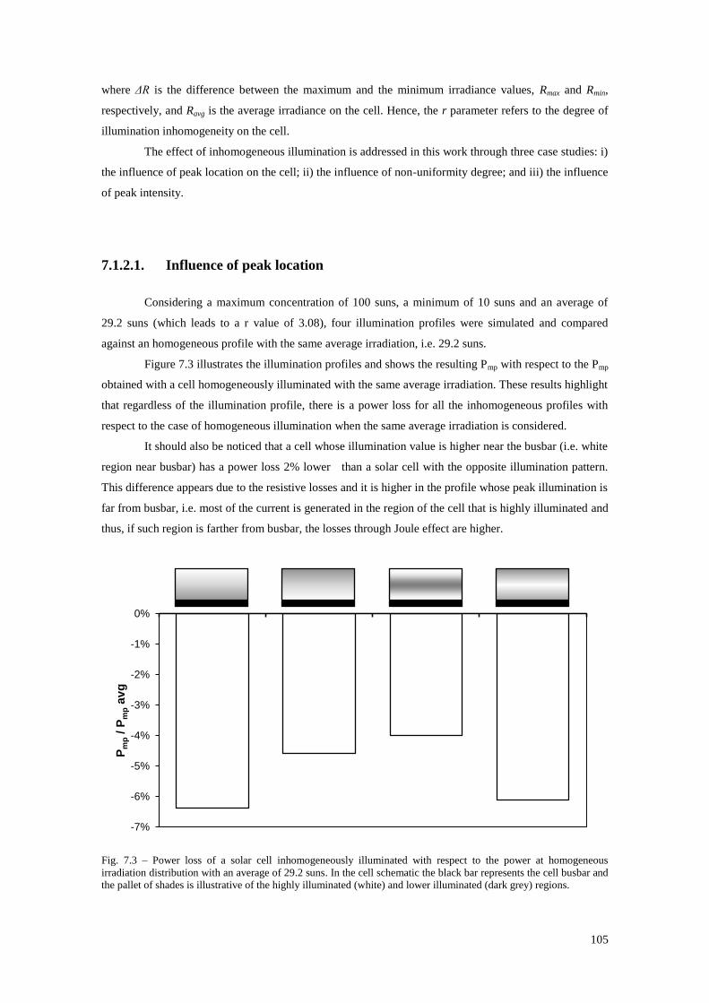
105

where ΔR is the difference between the maximum and the minimum irradiance values, Rmax and Rmin,

respectively, and Ravg is the average irradiance on the cell. Hence, the r parameter refers to the degree of

illumination inhomogeneity on the cell.

The effect of inhomogeneous illumination is addressed in this work through three case studies: i)

the influence of peak location on the cell; ii) the influence of non-uniformity degree; and iii) the influence

of peak intensity.

7.1.2.1. Influence of peak location

Considering a maximum concentration of 100 suns, a minimum of 10 suns and an average of

29.2 suns (which leads to a r value of 3.08), four illumination profiles were simulated and compared

against an homogeneous profile with the same average irradiation, i.e. 29.2 suns.

Figure 7.3 illustrates the illumination profiles and shows the resulting Pmp with respect to the Pmp

obtained with a cell homogeneously illuminated with the same average irradiation. These results highlight

that regardless of the illumination profile, there is a power loss for all the inhomogeneous profiles with

respect to the case of homogeneous illumination when the same average irradiation is considered.

It should also be noticed that a cell whose illumination value is higher near the busbar (i.e. white

region near busbar) has a power loss 2% lower than a solar cell with the opposite illumination pattern.

This difference appears due to the resistive losses and it is higher in the profile whose peak illumination is

far from busbar, i.e. most of the current is generated in the region of the cell that is highly illuminated and

thus, if such region is farther from busbar, the losses through Joule effect are higher.

Fig. 7.3 – Power loss of a solar cell inhomogeneously illuminated with respect to the power at homogeneous

irradiation distribution with an average of 29.2 suns. In the cell schematic the black bar represents the cell busbar and

the pallet of shades is illustrative of the highly illuminated (white) and lower illuminated (dark grey) regions.

-7%

-6%

-5%

-4%

-3%

-2%

-1%

0%

F1 F4 F7 F8

Pm

p / P

mp a

vg

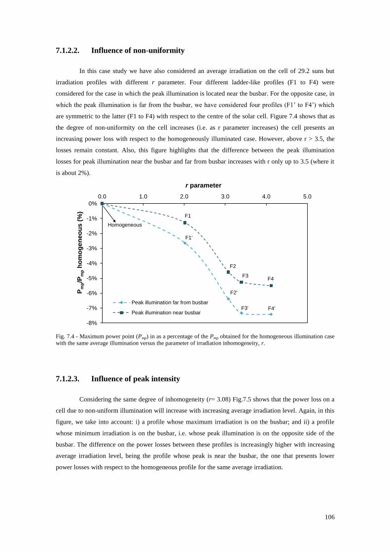
106

7.1.2.2. Influence of non-uniformity

In this case study we have also considered an average irradiation on the cell of 29.2 suns but

irradiation profiles with different r parameter. Four different ladder-like profiles (F1 to F4) were

considered for the case in which the peak illumination is located near the busbar. For the opposite case, in

which the peak illumination is far from the busbar, we have considered four profiles (F1’ to F4’) which

are symmetric to the latter (F1 to F4) with respect to the centre of the solar cell. Figure 7.4 shows that as

the degree of non-uniformity on the cell increases (i.e. as r parameter increases) the cell presents an

increasing power loss with respect to the homogeneously illuminated case. However, above r > 3.5, the

losses remain constant. Also, this figure highlights that the difference between the peak illumination

losses for peak illumination near the busbar and far from busbar increases with r only up to 3.5 (where it

is about 2%).

Fig. 7.4 - Maximum power point (Pmp) in as a percentage of the Pmp obtained for the homogeneous illumination case

with the same average illumination versus the parameter of irradiation inhomogeneity, r.

7.1.2.3. Influence of peak intensity

Considering the same degree of inhomogeneity (r= 3.08) Fig.7.5 shows that the power loss on a

cell due to non-uniform illumination will increase with increasing average irradiation level. Again, in this

figure, we take into account: i) a profile whose maximum irradiation is on the busbar; and ii) a profile

whose minimum irradiation is on the busbar, i.e. whose peak illumination is on the opposite side of the

busbar. The difference on the power losses between these profiles is increasingly higher with increasing

average irradiation level, being the profile whose peak is near the busbar, the one that presents lower

power losses with respect to the homogeneous profile for the same average irradiation.

F1'

F2'

F3' F4'

Homogeneous

F1

F2

F3 F4

-8%

-7%

-6%

-5%

-4%

-3%

-2%

-1%

0%

0.0 1.0 2.0 3.0 4.0 5.0

Pm

p/P

mp h

om

og

en

eo

us (

%)

r parameter

Peak illumination far from busbar

Peak illumination near busbar

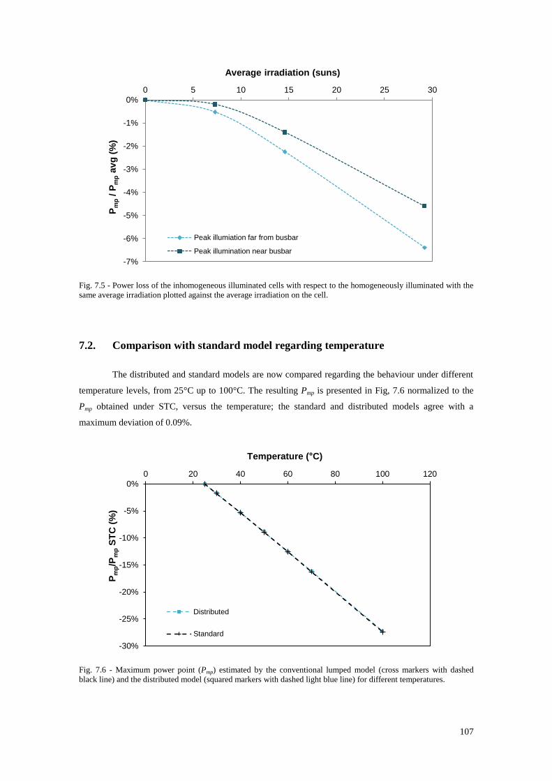
107

Fig. 7.5 - Power loss of the inhomogeneous illuminated cells with respect to the homogeneously illuminated with the

same average irradiation plotted against the average irradiation on the cell.

7.2. Comparison with standard model regarding temperature

The distributed and standard models are now compared regarding the behaviour under different

temperature levels, from 25°C up to 100°C. The resulting Pmp is presented in Fig, 7.6 normalized to the

Pmp obtained under STC, versus the temperature; the standard and distributed models agree with a

maximum deviation of 0.09%.

Fig. 7.6 - Maximum power point (Pmp) estimated by the conventional lumped model (cross markers with dashed

black line) and the distributed model (squared markers with dashed light blue line) for different temperatures.

-7%

-6%

-5%

-4%

-3%

-2%

-1%

0%

0 5 10 15 20 25 30

Pm

p / P

mp a

vg

(%

)

Average irradiation (suns)

Peak illumiation far from busbar

Peak illumination near busbar

-30%

-25%

-20%

-15%

-10%

-5%

0%

0 20 40 60 80 100 120

Pm

p/P

mp S

TC

(%

)

Temperature (°C)

Distributed

Standard

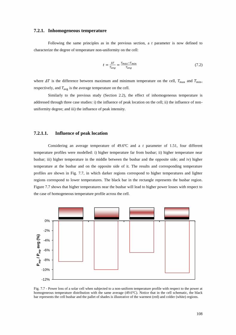
108

7.2.1. Inhomogeneous temperature

Following the same principles as in the previous section, a t parameter is now defined to

characterize the degree of temperature non-uniformity on the cell:

(7.2)

where is the difference between maximum and minimum temperature on the cell, and ,

respectively, and is the average temperature on the cell.

Similarly to the previous study (Section 2.2), the effect of inhomogeneous temperature is

addressed through three case studies: i) the influence of peak location on the cell; ii) the influence of non-

uniformity degree; and iii) the influence of peak intensity.

7.2.1.1. Influence of peak location

Considering an average temperature of 49.6ºC and a t parameter of 1.51, four different

temperature profiles were modelled: i) higher temperature far from busbar; ii) higher temperature near

busbar; iii) higher temperature in the middle between the busbar and the opposite side; and iv) higher

temperature at the busbar and on the opposite side of it. The results and corresponding temperature

profiles are shown in Fig. 7.7, in which darker regions correspond to higher temperatures and lighter

regions correspond to lower temperatures. The black bar in the rectangle represents the busbar region.

Figure 7.7 shows that higher temperatures near the busbar will lead to higher power losses with respect to

the case of homogeneous temperature profile across the cell.

Fig. 7.7 - Power loss of a solar cell when subjected to a non-uniform temperature profile with respect to the power at

homogeneous temperature distribution with the same average (49.6°C). Notice that in the cell schematic, the black

bar represents the cell busbar and the pallet of shades is illustrative of the warmest (red) and colder (white) regions.

-12%

-10%

-8%

-6%

-4%

-2%

0%

T3 T6 T7 T8

Pm

p / P

mp a

vg

(%

)

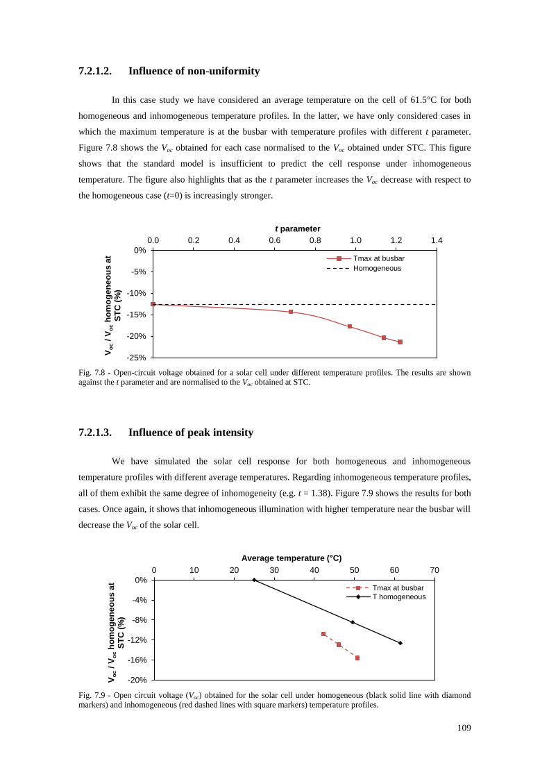
109

7.2.1.2. Influence of non-uniformity

In this case study we have considered an average temperature on the cell of 61.5°C for both

homogeneous and inhomogeneous temperature profiles. In the latter, we have only considered cases in

which the maximum temperature is at the busbar with temperature profiles with different t parameter.

Figure 7.8 shows the Voc obtained for each case normalised to the Voc obtained under STC. This figure

shows that the standard model is insufficient to predict the cell response under inhomogeneous

temperature. The figure also highlights that as the t parameter increases the Voc decrease with respect to

the homogeneous case (t=0) is increasingly stronger.

Fig. 7.8 - Open-circuit voltage obtained for a solar cell under different temperature profiles. The results are shown

against the t parameter and are normalised to the Voc obtained at STC.

7.2.1.3. Influence of peak intensity

We have simulated the solar cell response for both homogeneous and inhomogeneous

temperature profiles with different average temperatures. Regarding inhomogeneous temperature profiles,

all of them exhibit the same degree of inhomogeneity (e.g. t = 1.38). Figure 7.9 shows the results for both

cases. Once again, it shows that inhomogeneous illumination with higher temperature near the busbar will

decrease the Voc of the solar cell.

Fig. 7.9 - Open circuit voltage (Voc) obtained for the solar cell under homogeneous (black solid line with diamond

markers) and inhomogeneous (red dashed lines with square markers) temperature profiles.

-25%

-20%

-15%

-10%

-5%

0%

0.0 0.2 0.4 0.6 0.8 1.0 1.2 1.4

Vo

c / V

oc h

om

og

en

eo

us

at

ST

C (

%)

t parameter

Tmax at busbar

Homogeneous

-20%

-16%

-12%

-8%

-4%

0%

0 10 20 30 40 50 60 70

Vo

c / V

oc h

om

og

en

eo

us

at

ST

C (

%)

Average temperature (°C)

Tmax at busbar

T homogeneous

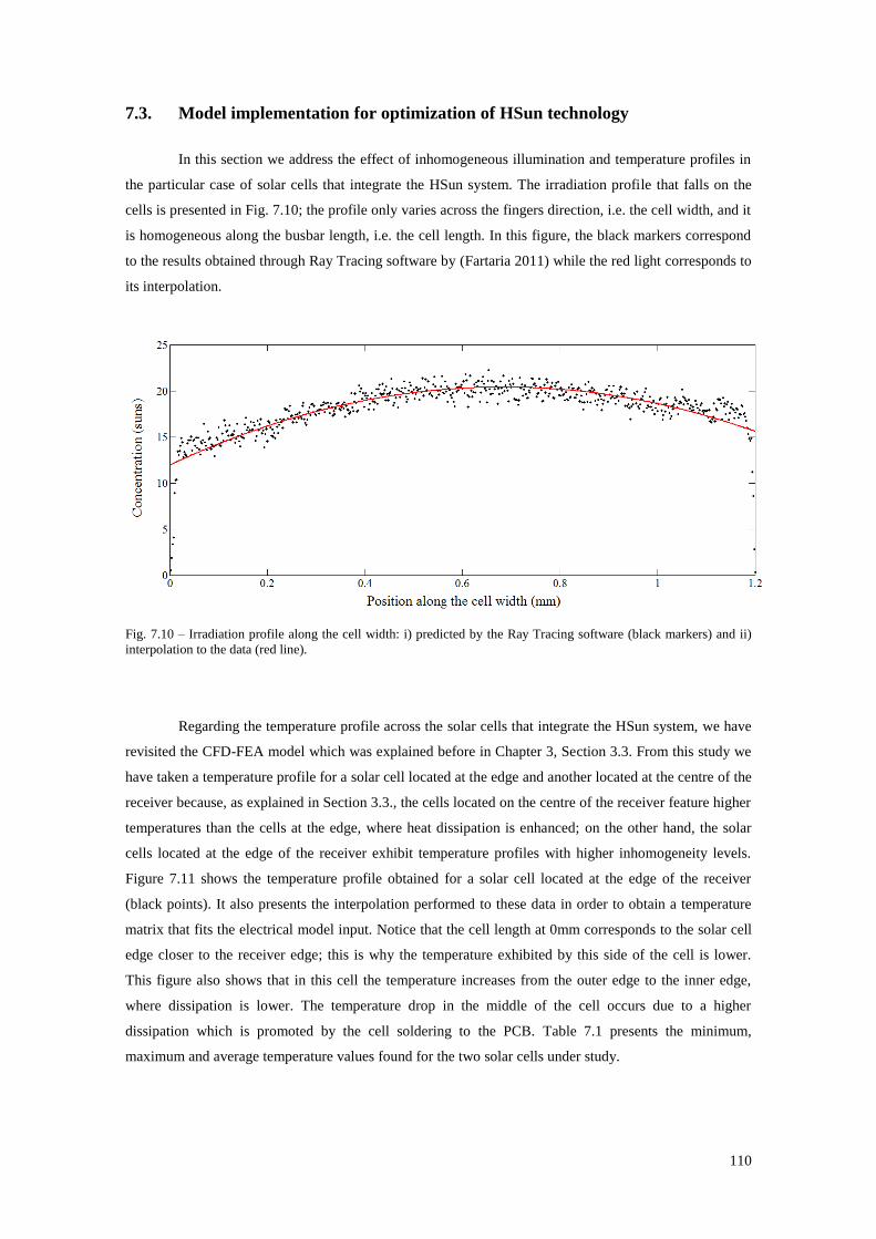
110

7.3. Model implementation for optimization of HSun technology

In this section we address the effect of inhomogeneous illumination and temperature profiles in

the particular case of solar cells that integrate the HSun system. The irradiation profile that falls on the

cells is presented in Fig. 7.10; the profile only varies across the fingers direction, i.e. the cell width, and it

is homogeneous along the busbar length, i.e. the cell length. In this figure, the black markers correspond

to the results obtained through Ray Tracing software by (Fartaria 2011) while the red light corresponds to

its interpolation.

Fig. 7.10 – Irradiation profile along the cell width: i) predicted by the Ray Tracing software (black markers) and ii)

interpolation to the data (red line).

Regarding the temperature profile across the solar cells that integrate the HSun system, we have

revisited the CFD-FEA model which was explained before in Chapter 3, Section 3.3. From this study we

have taken a temperature profile for a solar cell located at the edge and another located at the centre of the

receiver because, as explained in Section 3.3., the cells located on the centre of the receiver feature higher

temperatures than the cells at the edge, where heat dissipation is enhanced; on the other hand, the solar

cells located at the edge of the receiver exhibit temperature profiles with higher inhomogeneity levels.

Figure 7.11 shows the temperature profile obtained for a solar cell located at the edge of the receiver

(black points). It also presents the interpolation performed to these data in order to obtain a temperature

matrix that fits the electrical model input. Notice that the cell length at 0mm corresponds to the solar cell

edge closer to the receiver edge; this is why the temperature exhibited by this side of the cell is lower.

This figure also shows that in this cell the temperature increases from the outer edge to the inner edge,

where dissipation is lower. The temperature drop in the middle of the cell occurs due to a higher

dissipation which is promoted by the cell soldering to the PCB. Table 7.1 presents the minimum,

maximum and average temperature values found for the two solar cells under study.

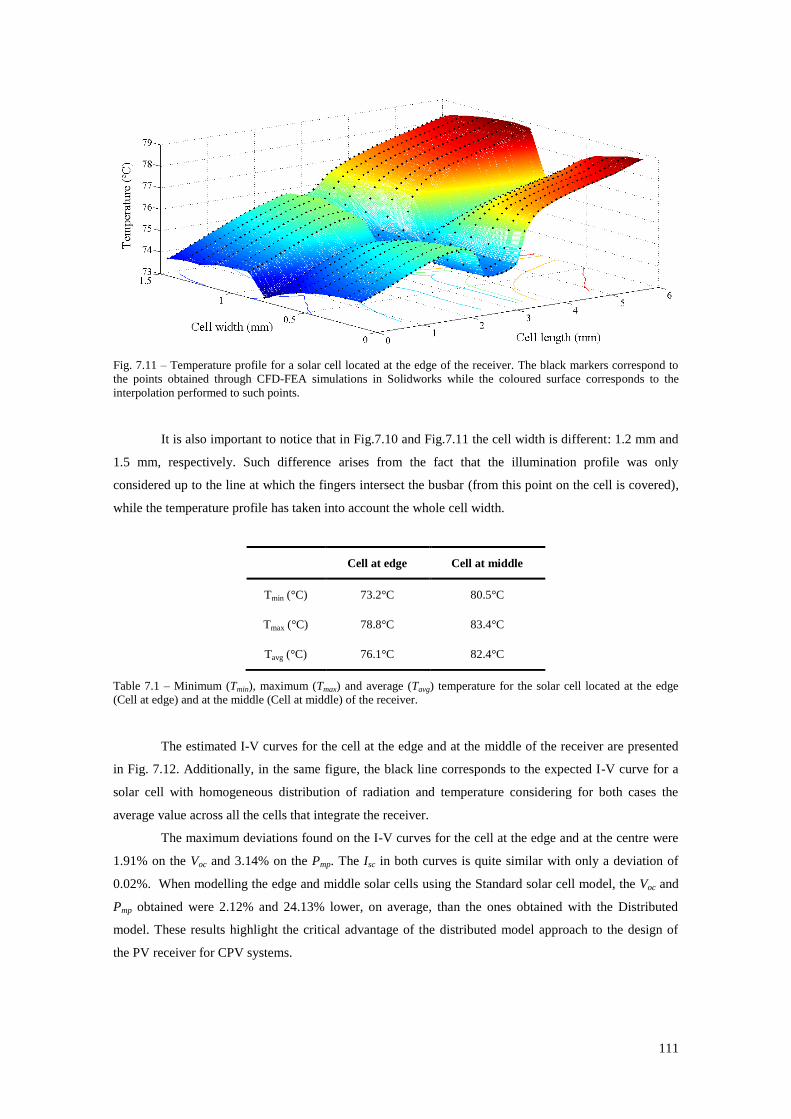
111

Fig. 7.11 – Temperature profile for a solar cell located at the edge of the receiver. The black markers correspond to

the points obtained through CFD-FEA simulations in Solidworks while the coloured surface corresponds to the

interpolation performed to such points.

It is also important to notice that in Fig.7.10 and Fig.7.11 the cell width is different: 1.2 mm and

1.5 mm, respectively. Such difference arises from the fact that the illumination profile was only

considered up to the line at which the fingers intersect the busbar (from this point on the cell is covered),

while the temperature profile has taken into account the whole cell width.

Cell at edge Cell at middle

Tmin (°C) 73.2°C 80.5°C

Tmax (°C) 78.8°C 83.4°C

Tavg (°C) 76.1°C 82.4°C

Table 7.1 – Minimum (Tmin), maximum (Tmax) and average (Tavg) temperature for the solar cell located at the edge

(Cell at edge) and at the middle (Cell at middle) of the receiver.

The estimated I-V curves for the cell at the edge and at the middle of the receiver are presented

in Fig. 7.12. Additionally, in the same figure, the black line corresponds to the expected I-V curve for a

solar cell with homogeneous distribution of radiation and temperature considering for both cases the

average value across all the cells that integrate the receiver.

The maximum deviations found on the I-V curves for the cell at the edge and at the centre were

1.91% on the Voc and 3.14% on the Pmp. The Isc in both curves is quite similar with only a deviation of

0.02%. When modelling the edge and middle solar cells using the Standard solar cell model, the Voc and

Pmp obtained were 2.12% and 24.13% lower, on average, than the ones obtained with the Distributed

model. These results highlight the critical advantage of the distributed model approach to the design of

the PV receiver for CPV systems.

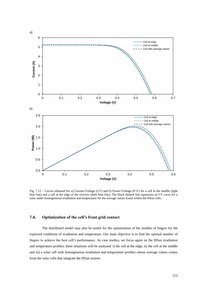
112

a)

b)

Fig. 7.12 – Curves obtained for a) Current-Voltage (I-V) and b) Power-Voltage (P-V) for a cell at the middle (light

blue line) and a cell at the edge of the receiver (dark blue line). The black dashed line represents an I-V curve for a

solar under homogeneous irradiation and temperature for the average values found within the HSun cells.

7.4. Optimization of the cell’s front grid contact

The distributed model may also be useful for the optimization of the number of fingers for the

expected conditions of irradiation and temperature. Our main objective is to find the optimal number of

fingers to achieve the best cell’s performance. As case studies, we focus again on the HSun irradiation

and temperature profiles; three situations will be analysed: i) the cell at the edge; ii) the cell at the middle

and iii) a solar cell with homogeneous irradiation and temperature profiles whose average values comes

from the solar cells that integrate the HSun system.

0

1

2

3

4

5

6

0 0.1 0.2 0.3 0.4 0.5 0.6 0.7

Cu

rre

nt

(A)

Voltage (V)

Cell at edge

Cell at middle

Cell with average values

0.0

0.5

1.0

1.5

2.0

2.5

0 0.1 0.2 0.3 0.4 0.5 0.6

Po

we

r (W

)

Voltage (V)

Cell at edge

Cell at middle

Cell with average values

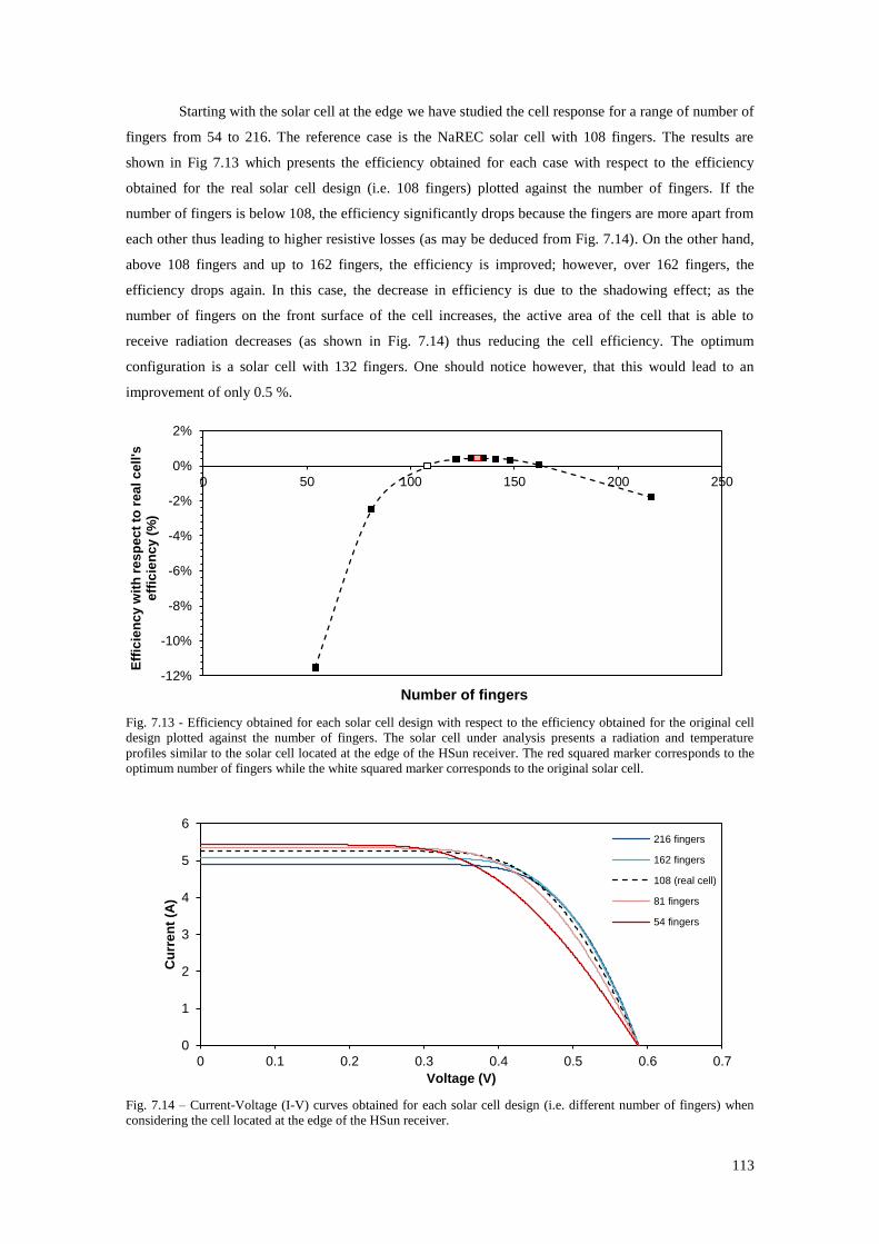
113

Starting with the solar cell at the edge we have studied the cell response for a range of number of

fingers from 54 to 216. The reference case is the NaREC solar cell with 108 fingers. The results are

shown in Fig 7.13 which presents the efficiency obtained for each case with respect to the efficiency

obtained for the real solar cell design (i.e. 108 fingers) plotted against the number of fingers. If the

number of fingers is below 108, the efficiency significantly drops because the fingers are more apart from

each other thus leading to higher resistive losses (as may be deduced from Fig. 7.14). On the other hand,

above 108 fingers and up to 162 fingers, the efficiency is improved; however, over 162 fingers, the

efficiency drops again. In this case, the decrease in efficiency is due to the shadowing effect; as the

number of fingers on the front surface of the cell increases, the active area of the cell that is able to

receive radiation decreases (as shown in Fig. 7.14) thus reducing the cell efficiency. The optimum

configuration is a solar cell with 132 fingers. One should notice however, that this would lead to an

improvement of only 0.5 %.

Fig. 7.13 - Efficiency obtained for each solar cell design with respect to the efficiency obtained for the original cell

design plotted against the number of fingers. The solar cell under analysis presents a radiation and temperature

profiles similar to the solar cell located at the edge of the HSun receiver. The red squared marker corresponds to the

optimum number of fingers while the white squared marker corresponds to the original solar cell.

Fig. 7.14 – Current-Voltage (I-V) curves obtained for each solar cell design (i.e. different number of fingers) when

considering the cell located at the edge of the HSun receiver.

-12%

-10%

-8%

-6%

-4%

-2%

0%

2%

0 50 100 150 200 250

Eff

icie

nc

y w

ith

res

pe

ct

to r

ea

l c

ell

's

eff

icie

nc

y (

%)

Number of fingers

0

1

2

3

4

5

6

0 0.1 0.2 0.3 0.4 0.5 0.6 0.7

Cu

rre

nt

(A)

Voltage (V)

216 fingers

162 fingers

108 (real cell)

81 fingers

54 fingers

114

For the other two case studies under analysis, e.g. the cell at the edge and the cell with average

temperature and irradiation profiles, the optimum number of fingers is also 132. Having the same number

of fingers for all the cells that integrate the PV receiver is an advantage since it allows benefiting from

economies of scale regarding cell production.

7.5. Conclusions

A distributed diode model to determine the performance of solar photovoltaic cells under non-

uniform irradiation and temperature distributions is thoroughly discussed and compared with the standard

lumped model.

In conditions of homogeneous illumination and temperature, the models show good agreement at

Standard Test Conditions and within a range of cell temperatures up to 100°C. On the other hand, at

higher irradiation levels, up to 30 suns, the standard lumped model deviates from the distributed model as

the concentration level increases. For the case study presented in this chapter, at 30 suns, the standard

lumped model features a maximum power point 29% below the Pmp of the distributed model. This

difference shows that, under concentrated irradiation, the lumped model overestimates the resistive losses

that occur on a solar cell since it considers that the total current generated on the cell passes through a

single lumped series resistance instead of, as modelled in the distributed approach, crossing a path with

different series resistance components that depend on the region where the current is generated. The

effect of temperature variation across the solar cell will also be misrepresented by the standard lumped

model. For the case study presented here, the standard model overestimates the Voc in 7% for a solar cell

with an average temperature of 50°C.

To describe the inhomogeneity of the illumination and temperature on the solar cell, the

inhomogeneity parameters r and t are defined. It is shown that, for the same average irradiation, sharper

illumination profiles (higher r) increase the power losses. This effect may reach 7.5% for the cases whose

maximum peak illumination is far from the busbar and 6% when the maximum peak illumination is near

the busbar. As far as temperature profiles are concerned, it was observed that increasing temperature

inhomogeneity leads to lower voltages. In the case study analysed, a 22% decrease in Voc was found for a

temperature distribution whose maximum peak temperature is near the busbar with respect to the STC

case.

For the HSun case study, it was found that cells’ efficiency may vary by 0.37% depending on its

location on the receiver. An optimization of the front grid solar cells design have determined that 132

fingers was the number that would optimize the solar cell’s efficiency for the temperature and radiation

conditions presented in the HSun technology.

115

References

Fartaria, T., 2011. Tolerance Study and Optical Optimization of a Concentrated Photovoltaic Module.,

Instituto Superior Técnico, Universidade Técnica de Lisboa.

Mitchell, K.W., 1977. Computer analysis of resistance and non-uniform illumination effects on

concentrator solar cells. In Tech. Dig. Int. Electron Devices Meet. Washington DC: IEEE, pp. 1–4.

Reis, F. et al., 2013. Modelling the effects of inhomogeneous irradiation and temperature profiles on CPV

cells behaviour. Paper submitted to IEEE Journal of Photovoltaics.

Schroder, D.K., 2006. Semiconductor Materials and Device Characterization 3rd ed., New Jersey: John

Wiley & Sons Ltd.

Serra, J.M., 1995. PhD thesis, University of Lisbon.

116

117

PART II

118

119

Introductory note

In the development of a new CPV system, such as the HSun technology (previously described in

Part I), it is crucial to understand the barriers and challenges that a real system may face during its

lifetime. One way to point out such issues is to look back for earlier developed CPV systems such as the

DoubleSun® technology, a two-axis low concentrator integrating standard PV modules and reflective

mirrors, developed by WS Energia.

In this context, before and along with the work developed the Part I, the DoubleSun® technology

was thoroughly explored and the analysis that were carried out are presented here in Part II, regarding: i)

system ageing; ii) on-field performance and challenges; iii) potential; and iv) cost of the generated

electricity.

Moreover, it should be noticed that the analysis of the electricity cost for a CPV system has

highlighted the need of a new CPV system, the HSun technology. This analysis has led to the

development of a Levelized Cost of Electricity (LCoE) model that was used as a tool when defining the

design of the HSun system.

120

121

Chapter 1 Ageing of DoubleSun® system

Concentration Photovoltaic (CPV) systems can only become competitive if, at least, they are

able to fulfil its production requirements during its operational life. Furthermore, since it has not reached

a large enough commercial scale to be considered mature, one of the barriers to its further dissemination

is bankability. In this context, ageing analysis of CPV systems is of paramount importance. This chapter

present an ageing study of the WS Energia earlier generation CPV system, the DoubleSun® technology, a

low concentration two-axis system with standard PV modules and reflective mirrors. The main objectives

of this work are:

To prepare the certification process of the DoubleSun® technology;

To understand/ identify the challenges of conventional silicon solar cells and encapsulation

materials when integrated in concentration systems; and

To understand the challenges that a new CPV system, such as the HSun technology, may face to

fulfil the requirements of a reliable PV system during its lifetime.

1.1. Introduction

From December of 2001 until December 2008 flat-plate PV modules were perceived as

extremely expensive, with average price above 4.5€/Wp (Company n.d.). At that time, as explained in

Part I, Chapter 1, Section 1.1, many CPV solutions arose as a shortcut to achieve lower photovoltaic

electricity cost/kWh. From the tested solutions, the V-trough arrangement was highlighted as a short term

solution mainly due to two main reasons: i) the optical configuration (reflective mirrors) allows high

homogeneity with moderate tracking accuracy avoiding prohibitively high costs of the final product; and

ii) the use of standard silicon solar cells, a technology with many years of given proofs and a well

standardized industrial manufacture, benefiting from scale production.

Based on these premises, the DoubleSun® technology, developed by WS Energia in 2006,

consisted of a 1.9x V-trough concentrator, with two flat mirrors (lightweight, highly reflective and

outdoor resistant) placed along the standard PV modules (high efficiency monocrystalline technology

with low temperature coefficient, since they are to operate under concentrated radiation), as shown in Fig.

1.1. The system integrates a two-axis tracking system with an annual power consumption that

corresponds to 0.3% of the annual expected system production (Reis et al. 2009).

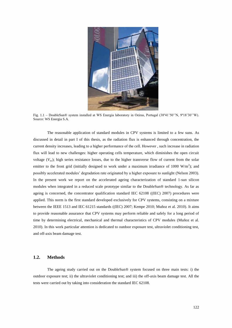
122

Fig. 1.1 – DoubleSun® system installed at WS Energia laboratory in Oeiras, Portugal (38º41’50’’N, 9º18’30’’W).

Source: WS Energia S.A.

The reasonable application of standard modules in CPV systems is limited to a few suns. As

discussed in detail in part I of this thesis, as the radiation flux is enhanced through concentration, the

current density increases, leading to a higher performance of the cell. However , such increase in radiation

flux will lead to new challenges: higher operating cells temperature, which diminishes the open circuit

voltage (Voc); high series resistance losses, due to the higher transverse flow of current from the solar

emitter to the front grid (initially designed to work under a maximum irradiance of 1000 W/m2); and

possibly accelerated modules’ degradation rate originated by a higher exposure to sunlight (Nelson 2003).

In the present work we report on the accelerated ageing characterization of standard 1-sun silicon

modules when integrated in a reduced scale prototype similar to the DoubleSun® technology. As far as

ageing is concerned, the concentrator qualification standard IEC 62108 ((IEC) 2007) procedures were

applied. This norm is the first standard developed exclusively for CPV systems, consisting on a mixture

between the IEEE 1513 and IEC 61215 standards ((IEC) 2007; Kempe 2010; Muñoz et al. 2010). It aims

to provide reasonable assurance that CPV systems may perform reliable and safely for a long period of

time by determining electrical, mechanical and thermal characteristics of CPV modules (Muñoz et al.

2010). In this work particular attention is dedicated to outdoor exposure test, ultraviolet conditioning test,

and off-axis beam damage test.

1.2. Methods

The ageing study carried out on the DoubleSun® system focused on three main tests: i) the

outdoor exposure test; ii) the ultraviolet conditioning test; and iii) the off-axis beam damage test. All the

tests were carried out by taking into consideration the standard IEC 62108.

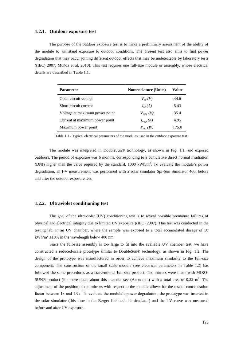
123

1.2.1. Outdoor exposure test

The purpose of the outdoor exposure test is to make a preliminary assessment of the ability of

the module to withstand exposure to outdoor conditions. The present test also aims to find power

degradation that may occur joining different outdoor effects that may be undetectable by laboratory tests

((IEC) 2007; Muñoz et al. 2010). This test requires one full-size module or assembly, whose electrical

details are described in Table 1.1.

Parameter Nomenclature (Units) Value

Open-circuit voltage Voc (V) 44.6

Short-circuit current Isc (A) 5.43

Voltage at maximum power point Vmpp (V) 35.4

Current at maximum power point Impp (A) 4.95

Maximum power point Pmp (W) 175.0

Table 1.1 - Typical electrical parameters of the modules used in the outdoor exposure test.

The module was integrated in DoubleSun® technology, as shown in Fig. 1.1, and exposed

outdoors. The period of exposure was 6 months, corresponding to a cumulative direct normal irradiation

(DNI) higher than the value required by the standard, 1000 kWh/m2. To evaluate the module’s power

degradation, an I-V measurement was performed with a solar simulator Spi-Sun Simulator 460i before

and after the outdoor exposure test.

1.2.2. Ultraviolet conditioning test

The goal of the ultraviolet (UV) conditioning test is to reveal possible premature failures of

physical and electrical integrity due to limited UV exposure ((IEC) 2007). This test was conducted in the

testing lab, in an UV chamber, where the sample was exposed to a total accumulated dosage of 50

kWh/m2 ±10% in the wavelength below 400 nm.

Since the full-size assembly is too large to fit into the available UV chamber test, we have

constructed a reduced-scale prototype similar to DoubleSun® technology, as shown in Fig. 1.2. The

design of the prototype was manufactured in order to achieve maximum similarity to the full-size

component. The construction of the small scale module (see electrical parameters in Table 1.2) has

followed the same procedures as a conventional full-size product. The mirrors were made with MIRO-

SUN® product (for more detail about this material see (Anon n.d.) with a total area of 0.22 m2. The

adjustment of the position of the mirrors with respect to the module allows for the test of concentration

factor between 1x and 1.9x. To evaluate the module’s power degradation, the prototype was inserted in

the solar simulator (this time in the Berger Lichttechnik simulator) and the I-V curve was measured

before and after UV exposure.

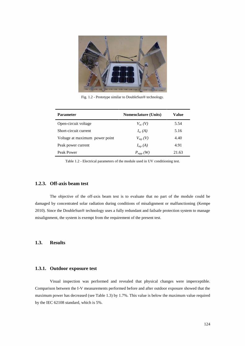
124

Fig. 1.2 - Prototype similar to DoubleSun® technology.

Parameter Nomenclature (Units) Value

Open-circuit voltage Voc (V) 5.54

Short-circuit current Isc (A) 5.16

Voltage at maximum power point Vmp (V) 4.40

Peak power current Imp (A) 4.91

Peak Power Pmpp (W) 21.63

Table 1.2 - Electrical parameters of the module used in UV conditioning test.

1.2.3. Off-axis beam test

The objective of the off-axis beam test is to evaluate that no part of the module could be

damaged by concentrated solar radiation during conditions of misalignment or malfunctioning (Kempe

2010). Since the DoubleSun® technology uses a fully redundant and failsafe protection system to manage

misalignment, the system is exempt from the requirement of the present test.

1.3. Results

1.3.1. Outdoor exposure test

Visual inspection was performed and revealed that physical changes were imperceptible.

Comparison between the I-V measurements performed before and after outdoor exposure showed that the

maximum power has decreased (see Table 1.3) by 1.7%. This value is below the maximum value required

by the IEC 62108 standard, which is 5%.

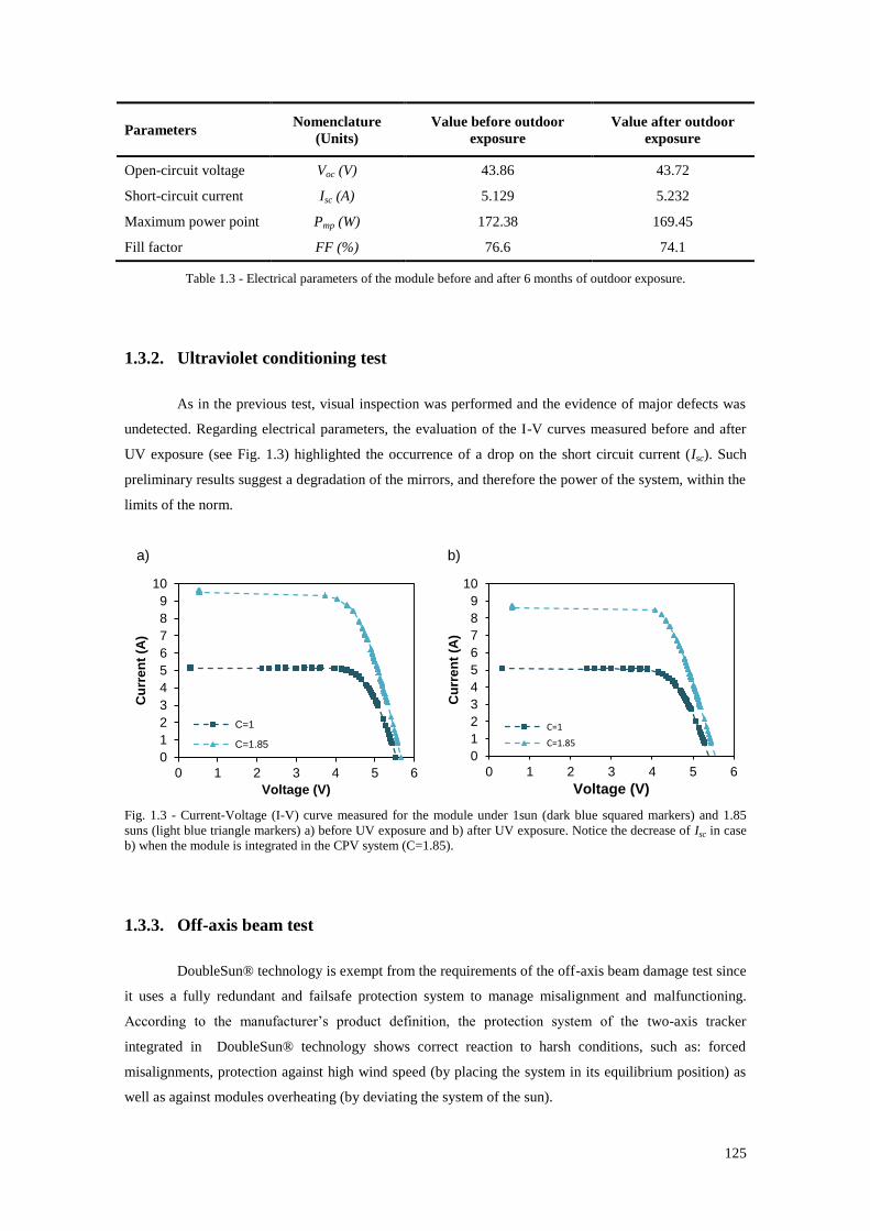
125

Parameters Nomenclature

(Units)

Value before outdoor

exposure

Value after outdoor

exposure

Open-circuit voltage Voc (V) 43.86 43.72

Short-circuit current Isc (A) 5.129 5.232

Maximum power point Pmp (W) 172.38 169.45

Fill factor FF (%) 76.6 74.1

Table 1.3 - Electrical parameters of the module before and after 6 months of outdoor exposure.

1.3.2. Ultraviolet conditioning test

As in the previous test, visual inspection was performed and the evidence of major defects was

undetected. Regarding electrical parameters, the evaluation of the I-V curves measured before and after

UV exposure (see Fig. 1.3) highlighted the occurrence of a drop on the short circuit current (Isc). Such

preliminary results suggest a degradation of the mirrors, and therefore the power of the system, within the

limits of the norm.

a) b)

Fig. 1.3 - Current-Voltage (I-V) curve measured for the module under 1sun (dark blue squared markers) and 1.85

suns (light blue triangle markers) a) before UV exposure and b) after UV exposure. Notice the decrease of Isc in case

b) when the module is integrated in the CPV system (C=1.85).

1.3.3. Off-axis beam test

DoubleSun® technology is exempt from the requirements of the off-axis beam damage test since

it uses a fully redundant and failsafe protection system to manage misalignment and malfunctioning.

According to the manufacturer’s product definition, the protection system of the two-axis tracker

integrated in DoubleSun® technology shows correct reaction to harsh conditions, such as: forced

misalignments, protection against high wind speed (by placing the system in its equilibrium position) as

well as against modules overheating (by deviating the system of the sun).

0

1

2

3

4

5

6

7

8

9

10

0 1 2 3 4 5 6

Cu

rre

nt

(A)

Voltage (V)

C=1

C=1.85

0

1

2

3

4

5

6

7

8

9

10

0 1 2 3 4 5 6

Cu

rre

nt

(A)

Voltage (V)

C=1

C=1.85

126

1.4. Conclusions

Outdoor exposure, with DNI higher than 1000 kWh/m2, showed that standard silicon modules

undergo 1.7% of power degradation when integrated in a V-trough system with 1.9x concentration.

Preliminary results of ultraviolet exposure, under lab conditions and with a reduced-scale

prototype, have shown a decrease of the short-circuit current, suggesting a decrease on the concentration

factor due to mirrors degradation. However, power degradation remains within the requirements of the

norm. Major physical defects of the assembly were unnoticed in both previous tests. DoubleSun® system

may be exempt of the off-axis beam test, since all the requirements and manufacturer’s specification were

previously verified.

The successful results of the tests performed according to the IEC62108 standard suggest that,

for the range of concentration factors tested, standard silicon modules may be eligible for concentration.

The present work provides reasonable assurance of system reliability for a long period of time and opens

the path for product successful certification according to the IEC 62108 standard.

References

(IEC), I.E.C., 2007. IEC 62108: Concentrator Photovoltaic (CPV) modules and assemblies - Design

qualification and type approval 1st ed., USA.

Anon, Alanod solar. Available at: http://www.alanod-

solar.com/opencms/opencms/Reflexion/Produkte.html.

Company, N.G., Solarbuzz - Solar Market Research and Analysis. Available at:

http://www.solarbuzz.com/facts-and-figures/retail-price-environment/module-prices.

Kempe, M.D., 2010. Ultraviolet light test and evaluation methods for encapsulants of photovoltaic

modules. Solar Energy Materials and Solar Cells, 94(2), pp.246–253. Available at:

http://linkinghub.elsevier.com/retrieve/pii/S0927024809003274 [Accessed March 12, 2013].

Muñoz, E. et al., 2010. CPV standardization: An overview. Renewable and Sustainable Energy Reviews,

14(1), pp.518–523. Available at: http://linkinghub.elsevier.com/retrieve/pii/S1364032109001701

[Accessed March 12, 2013].

Nelson, J., 2003. The Physics of Solar Cells 1st ed., London, UK: Imperial College Press.

Reis, F. et al., 2009. Power Generation and Energy Yield using Doublesun Photovoltaic Solar

Concentration. Proc. 24th EU PVSEC, Hamburg, Germany, pp.803–806. Available at:

http://solar.fc.ul.pt/lafspapers/1DV537.pdf [Accessed January 31, 2012].

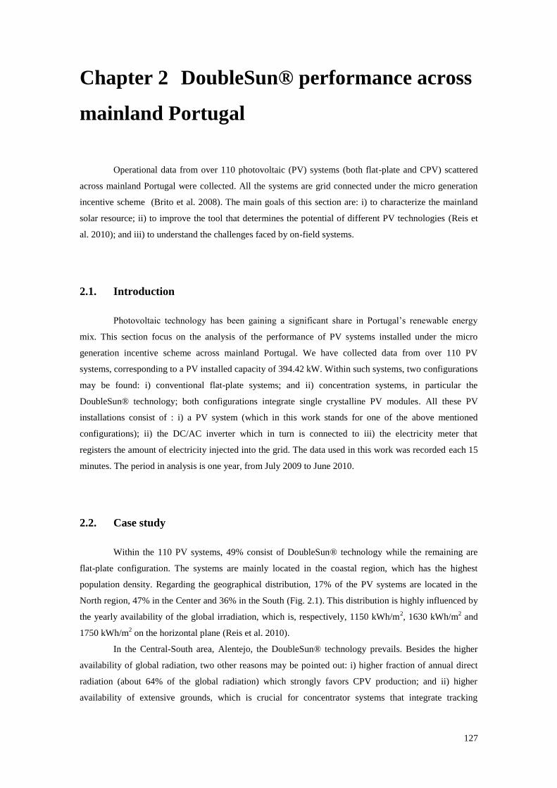
127

Chapter 2 DoubleSun® performance across

mainland Portugal

Operational data from over 110 photovoltaic (PV) systems (both flat-plate and CPV) scattered

across mainland Portugal were collected. All the systems are grid connected under the micro generation

incentive scheme (Brito et al. 2008). The main goals of this section are: i) to characterize the mainland

solar resource; ii) to improve the tool that determines the potential of different PV technologies (Reis et

al. 2010); and iii) to understand the challenges faced by on-field systems.

2.1. Introduction

Photovoltaic technology has been gaining a significant share in Portugal’s renewable energy

mix. This section focus on the analysis of the performance of PV systems installed under the micro

generation incentive scheme across mainland Portugal. We have collected data from over 110 PV

systems, corresponding to a PV installed capacity of 394.42 kW. Within such systems, two configurations

may be found: i) conventional flat-plate systems; and ii) concentration systems, in particular the

DoubleSun® technology; both configurations integrate single crystalline PV modules. All these PV

installations consist of : i) a PV system (which in this work stands for one of the above mentioned

configurations); ii) the DC/AC inverter which in turn is connected to iii) the electricity meter that

registers the amount of electricity injected into the grid. The data used in this work was recorded each 15

minutes. The period in analysis is one year, from July 2009 to June 2010.

2.2. Case study

Within the 110 PV systems, 49% consist of DoubleSun® technology while the remaining are

flat-plate configuration. The systems are mainly located in the coastal region, which has the highest

population density. Regarding the geographical distribution, 17% of the PV systems are located in the

North region, 47% in the Center and 36% in the South (Fig. 2.1). This distribution is highly influenced by

the yearly availability of the global irradiation, which is, respectively, 1150 kWh/m2, 1630 kWh/m

2 and

1750 kWh/m2 on the horizontal plane (Reis et al. 2010).

In the Central-South area, Alentejo, the DoubleSun® technology prevails. Besides the higher

availability of global radiation, two other reasons may be pointed out: i) higher fraction of annual direct

radiation (about 64% of the global radiation) which strongly favors CPV production; and ii) higher

availability of extensive grounds, which is crucial for concentrator systems that integrate tracking

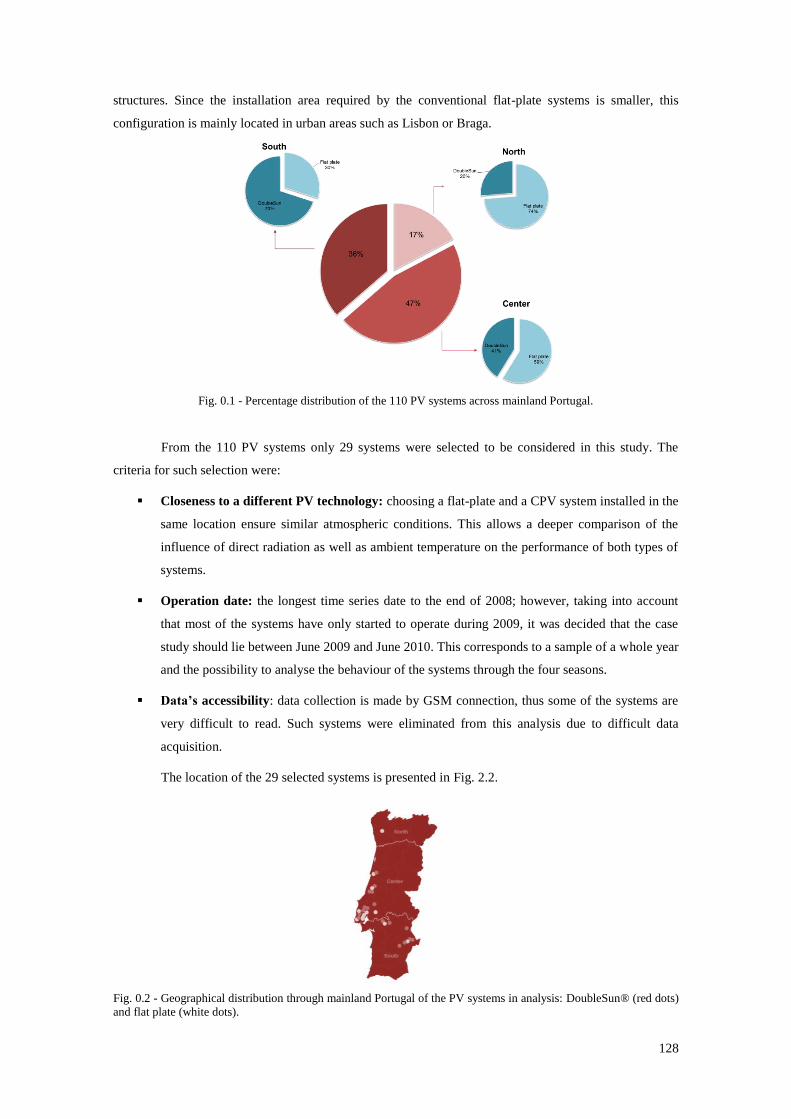
128

structures. Since the installation area required by the conventional flat-plate systems is smaller, this

configuration is mainly located in urban areas such as Lisbon or Braga.

Fig. 0.1 - Percentage distribution of the 110 PV systems across mainland Portugal.

From the 110 PV systems only 29 systems were selected to be considered in this study. The

criteria for such selection were:

Closeness to a different PV technology: choosing a flat-plate and a CPV system installed in the

same location ensure similar atmospheric conditions. This allows a deeper comparison of the

influence of direct radiation as well as ambient temperature on the performance of both types of

systems.

Operation date: the longest time series date to the end of 2008; however, taking into account

that most of the systems have only started to operate during 2009, it was decided that the case

study should lie between June 2009 and June 2010. This corresponds to a sample of a whole year

and the possibility to analyse the behaviour of the systems through the four seasons.

Data’s accessibility: data collection is made by GSM connection, thus some of the systems are

very difficult to read. Such systems were eliminated from this analysis due to difficult data

acquisition.

The location of the 29 selected systems is presented in Fig. 2.2.

Fig. 0.2 - Geographical distribution through mainland Portugal of the PV systems in analysis: DoubleSun® (red dots)

and flat plate (white dots).

129

2.3. Systems performance

2.3.1. Annual energy

During the period in analysis, July 2009 to June 2010, the average annual production of the

DoubleSun® systems was 2151.59 kWh/kWp, exceeding in 48% the average annual production

registered for the conventional flat plate systems (Fig. 2.3). This energy excess occurs mainly during the

summer months (i.e. months with significantly higher percentage of direct radiation).

Fig. 0.3 – Accumulated energy produced by the DoubleSun® (squared markers) and a flat-plate (triangle markers)

system from July 2009 to June 2010. In the up left corner the average annual energy produced by each system during

the period under analysis is presented with respect to the flat-plate system annual energy.

Figure 2.4.a) shows that DoubleSun® technology may produce up to 350 kWh/kWp/month in

the summer while the conventional flat-plate systems (Figure 2.4.b)) achieve a maximum value of 200

kWh/kWp/month. However, during the winter, due to the higher fraction of cloudy days, and

consequently higher percentage of diffuse radiation, the production of both technologies is similar;

nevertheless, the DoubleSun® systems reached higher values taking advantage of the clear days in

winter.

The relevance of the direct radiation on CPV systems performance is noticeable in Figure 2.4,

which shows that the DoubleSun® systems installed on the southern regions (higher percentage of direct

radiation) are likely to produce higher amount of energy than the systems in the northern regions (lower

percentage of direct radiation).

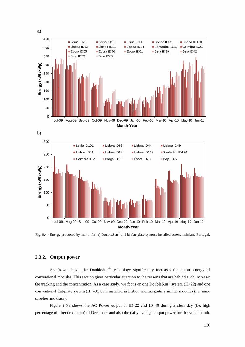
130

a)

b)

Fig. 0.4 - Energy produced by month for: a) DoubleSun® and b) flat-plate systems installed across mainland Portugal.

2.3.2. Output power

As shown above, the DoubleSun® technology significantly increases the output energy of

conventional modules. This section gives particular attention to the reasons that are behind such increase:

the tracking and the concentration. As a case study, we focus on one DoubleSun® system (ID 22) and one

conventional flat-plate system (ID 49), both installed in Lisbon and integrating similar modules (i.e. same

supplier and class).

Figure 2.5.a shows the AC Power output of ID 22 and ID 49 during a clear day (i.e. high

percentage of direct radiation) of December and also the daily average output power for the same month.

0

50

100

150

200

250

300

350

400

450

Jul-09 Aug-09 Sep-09 Oct-09 Nov-09 Dec-09 Jan-10 Feb-10 Mar-10 Apr-10 May-10 Jun-10

En

erg

y (

kW

h/k

Wp

)

Month-Year

Leiria ID70 Leiria ID50 Leiria ID14 Lisboa ID52 Lisboa ID110

Lisboa ID12 Lisboa ID22 Lisboa ID24 Santarém ID15 Coimbra ID21

Évora ID55 Évora ID56 Évora ID61 Beja ID39 Beja ID42

Beja ID79 Beja ID85

0

50

100

150

200

250

300

Jul-09 Aug-09 Sep-09 Oct-09 Nov-09 Dec-09 Jan-10 Feb-10 Mar-10 Apr-10 May-10 Jun-10

En

erg

y (

kW

h/k

Wp

)

Month-Year

Leiria ID101 Lisboa ID99 Lisboa ID44 Lisboa ID49

Lisboa ID51 Lisboa ID68 Lisboa ID122 Santarém ID120

Coimbra ID25 Braga ID103 Évora ID73 Beja ID72

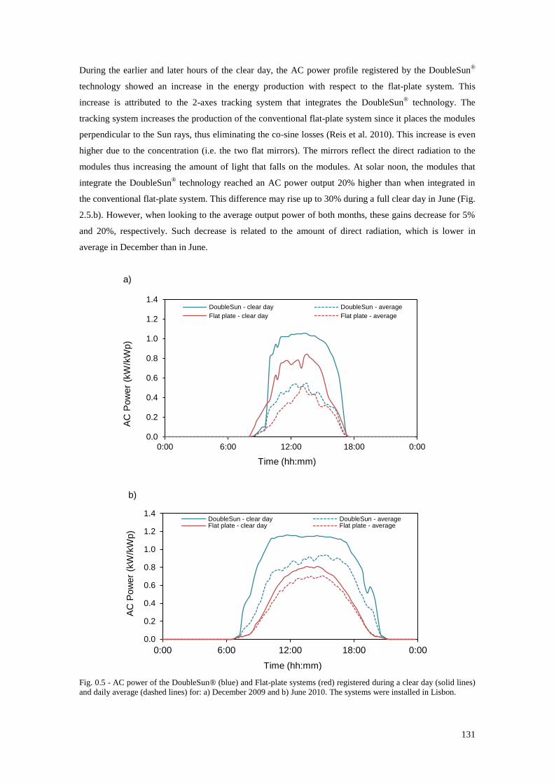
131

During the earlier and later hours of the clear day, the AC power profile registered by the DoubleSun®

technology showed an increase in the energy production with respect to the flat-plate system. This

increase is attributed to the 2-axes tracking system that integrates the DoubleSun® technology. The

tracking system increases the production of the conventional flat-plate system since it places the modules

perpendicular to the Sun rays, thus eliminating the co-sine losses (Reis et al. 2010). This increase is even

higher due to the concentration (i.e. the two flat mirrors). The mirrors reflect the direct radiation to the

modules thus increasing the amount of light that falls on the modules. At solar noon, the modules that

integrate the DoubleSun® technology reached an AC power output 20% higher than when integrated in

the conventional flat-plate system. This difference may rise up to 30% during a full clear day in June (Fig.

2.5.b). However, when looking to the average output power of both months, these gains decrease for 5%

and 20%, respectively. Such decrease is related to the amount of direct radiation, which is lower in

average in December than in June.

a)

b)

Fig. 0.5 - AC power of the DoubleSun® (blue) and Flat-plate systems (red) registered during a clear day (solid lines)

and daily average (dashed lines) for: a) December 2009 and b) June 2010. The systems were installed in Lisbon.

0.0

0.2

0.4

0.6

0.8

1.0

1.2

1.4

0:00 6:00 12:00 18:00 0:00

AC

Pow

er

(kW

/kW

p)

Time (hh:mm)

DoubleSun - clear day DoubleSun - average

Flat plate - clear day Flat plate - average

0.0

0.2

0.4

0.6

0.8

1.0

1.2

1.4

0:00 6:00 12:00 18:00 0:00

AC

Pow

er

(kW

/kW

p)

Time (hh:mm)

DoubleSun - clear day DoubleSun - averageFlat plate - clear day Flat plate - average

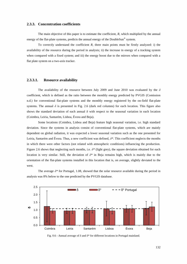
132

2.3.3. Concentration coefficients

The main objective of this paper is to estimate the coefficient, R, which multiplied by the annual

energy of the flat-plate systems, predicts the annual energy of the DoubleSun® system.

To correctly understand the coefficient R, three main points must be firstly analyzed: i) the

availability of the resource during the period in analysis; ii) the increase in energy of a tracking system

when compared with a fixed system; and iii) the energy boost due to the mirrors when compared with a

flat plate system on a two-axis tracker.

2.3.3.1. Resource availability

The availability of the resource between July 2009 and June 2010 was evaluated by the δ

coefficient, which is defined as the ratio between the monthly energy predicted by PVGIS (Comission

n.d.) for conventional flat-plate systems and the monthly energy registered by the on-field flat-plate

systems. The annual δ is presented in Fig. 2.6 (dark red columns) for each location. This figure also

shows the standard deviation of each annual δ with respect to the seasonal variation in each location

(Coimbra, Leiria, Santarém, Lisboa, Évora and Beja).

Some locations (Coimbra, Lisboa and Beja) feature high seasonal variation, i.e. high standard

deviation. Since the systems in analysis consist of conventional flat-plate systems, which are mainly

dependent on global radiation, it was expected a lower seasonal variation such as the one presented for

Leiria, Santarém and Évora. Thus, a new coefficient was defined, δ*. This coefficient neglects the months

in which there were other factors (not related with atmospheric conditions) influencing the production.

Figure 2.6 shows that neglecting such months, i.e. δ* (light grey), the square deviation obtained for each

location is very similar. Still, the deviation of δ* in Beja remains high, which is mainly due to the

orientation of the flat-plate systems installed in this location that is, on average, slightly deviated to the

west.

The average δ* for Portugal, 1.08, showed that the solar resource available during the period in

analysis was 8% below to the one predicted by the PVGIS database.

Fig. 0.6 - Annual average of δ and δ* for different locations in Portugal mainland.

0.0

0.5

1.0

1.5

2.0

2.5

Coimbra Leiria Santarém Lisboa Évora Beja

δ

δ δ* δ* Portugal

133

2.3.3.2. Energy increase due to tracking

The percentage of direct radiation strongly influences the performance of a CPV system. To

evaluate such parameter the γ coefficient was defined as the ratio between the monthly energy estimated

for a two-axis tracking system and the monthly energy estimated for a conventional flat-plate system.

Those values were taken from the PVGIS database (Comission n.d.) due to the absence of two-axis

tracking systems (without concentration) within the 29 systems in analysis.

The annual average of γ and the annual average ratio between direct irradiation and global

irradiation (ic) are presented in Fig. 2.7, for each location. The analysis of this figure shows that the γ

coefficient tends to increase from the North (Coimbra) to the South (Beja). This increase is related to the

increase of the percentage of direct radiation in the global radiation (ic). The tracking systems point the

modules to the Sun; however they are only effective if the radiation comes directly from the Sun, i.e.

without being scattered by clouds. Regarding the seasonal variability of the direct radiation, it seems very

similar for all the locations.

Fig. 0.7 - Annual average of γ for different locations in Portugal mainland.

2.3.3.3. Energy increase due to mirrors

To evaluate the energy boost due to the mirrors, we define an α coefficient as the ratio between

the monthly energy produced by the DoubleSun® system and the monthly energy predicted by PVGIS

(Comission n.d.) for a two-axis tracking system. As in the δ ratio, we have defined an α* which neglects

the months with reduced production due to other factors than atmospheric conditions.

Figure 2.8 shows the average annual α* obtained for each location. This figure shows that α*

tends to be decreased from North to South. This behavior is opposite to the increase of the direct

radiation. This situation highlights that the energy boost in concentration is also affected by the module

temperature, which is lower in the North and higher in the South. Moreover, the temperature of the

module will increase with increasing amount of radiation being redirected by the mirrors to the modules.

It is also important to notice that the seasonal variation (represented by the standard deviation

error bar) of the direct radiation is higher in the North than in the South.

0.0

0.2

0.4

0.6

0.8

1.0

1.2

1.4

1.6

Coimbra Leiria Santarém Lisboa Évora Beja

γ

γ γ Portugal

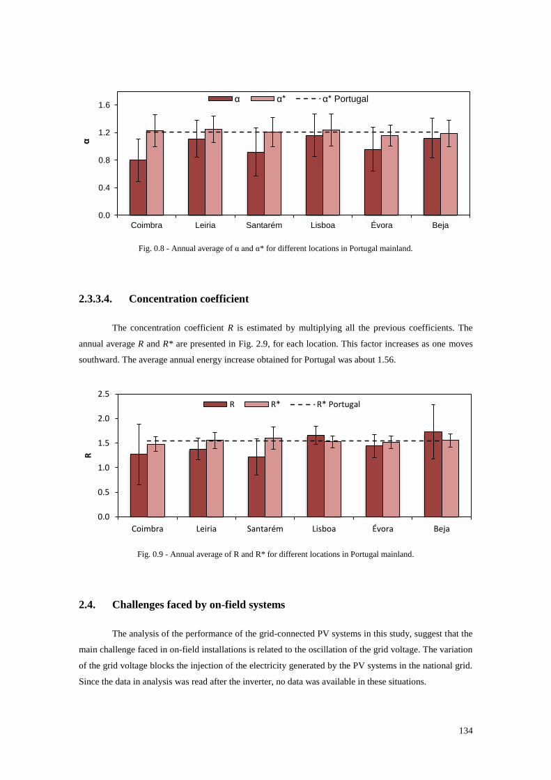
134

Fig. 0.8 - Annual average of α and α* for different locations in Portugal mainland.

2.3.3.4. Concentration coefficient

The concentration coefficient R is estimated by multiplying all the previous coefficients. The

annual average R and R* are presented in Fig. 2.9, for each location. This factor increases as one moves

southward. The average annual energy increase obtained for Portugal was about 1.56.

Fig. 0.9 - Annual average of R and R* for different locations in Portugal mainland.

2.4. Challenges faced by on-field systems

The analysis of the performance of the grid-connected PV systems in this study, suggest that the

main challenge faced in on-field installations is related to the oscillation of the grid voltage. The variation

of the grid voltage blocks the injection of the electricity generated by the PV systems in the national grid.

Since the data in analysis was read after the inverter, no data was available in these situations.

0.0

0.4

0.8

1.2

1.6

Coimbra Leiria Santarém Lisboa Évora Beja

α

α α* α* Portugal

0.0

0.5

1.0

1.5

2.0

2.5

Coimbra Leiria Santarém Lisboa Évora Beja

R

R R* R* Portugal

135

The CPV systems under analysis also feature occasional tracking misalignment. The average

energy increase of the DoubleSun® system with respect to the conventional flat-plate systems was

estimated in 1.45. This factor increases up to 1.54 when neglecting the months with tracking

misalignment and absence of data (i.e. other factors not related with atmospheric conditions). Thus

tracking errors may lead, at most, a 6% loss of energy production.

2.5. Conclusions

During the period in analysis, July 2009 – June 2010, the conventional flat-plate systems have

produced less 8% than the annual energy estimated by the PVGIS database, due to an unusually less

favorable year.

The on-field evaluation has clearly shown that, in Portugal, the DoubleSun® technology may

increase by a factor of 1.56 the average annual energy of conventional modules. For clear days and near

solar noon, the DoubleSun® technology has an AC output power that exceeds in 20% and 40% the

production of the conventional flat-plate systems in Winter and Summer, respectively. During the earlier

and later hours of summer days, DoubleSun® technology may achieve twice the production of

conventional flat-plate systems.

References

Brito, M.C. et al., 2008. Evaluation of the implementation of PV Feed-in law in Portugal. In 24th

EUPVSEC. Hamburg, Germany, pp. 1–3.

Comission, J.E., Photovoltaic Geographical Information System - Interactive Maps. Available at:

http://re.jrc.ec.europa.eu/pvgis/apps4/pvest.php#.

Reis, F. et al., 2010. Modeling the performance of low concentration photovoltaic systems. Solar Energy

Materials and Solar Cells, 94(7), pp.1222–1226. Available at:

http://linkinghub.elsevier.com/retrieve/pii/S0927024810001376 [Accessed January 31, 2012].

136

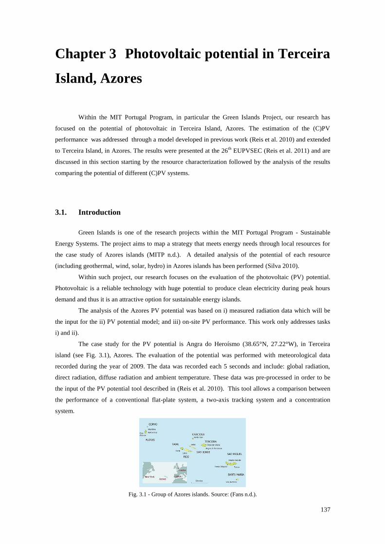
137

Chapter 3 Photovoltaic potential in Terceira

Island, Azores

Within the MIT Portugal Program, in particular the Green Islands Project, our research has

focused on the potential of photovoltaic in Terceira Island, Azores. The estimation of the (C)PV

performance was addressed through a model developed in previous work (Reis et al. 2010) and extended

to Terceira Island, in Azores. The results were presented at the 26th

EUPVSEC (Reis et al. 2011) and are

discussed in this section starting by the resource characterization followed by the analysis of the results

comparing the potential of different (C)PV systems.

3.1. Introduction

Green Islands is one of the research projects within the MIT Portugal Program - Sustainable

Energy Systems. The project aims to map a strategy that meets energy needs through local resources for

the case study of Azores islands (MITP n.d.). A detailed analysis of the potential of each resource

(including geothermal, wind, solar, hydro) in Azores islands has been performed (Silva 2010).

Within such project, our research focuses on the evaluation of the photovoltaic (PV) potential.

Photovoltaic is a reliable technology with huge potential to produce clean electricity during peak hours

demand and thus it is an attractive option for sustainable energy islands.

The analysis of the Azores PV potential was based on i) measured radiation data which will be

the input for the ii) PV potential model; and iii) on-site PV performance. This work only addresses tasks

i) and ii).

The case study for the PV potential is Angra do Heroísmo (38.65°N, 27.22°W), in Terceira

island (see Fig. 3.1), Azores. The evaluation of the potential was performed with meteorological data

recorded during the year of 2009. The data was recorded each 5 seconds and include: global radiation,

direct radiation, diffuse radiation and ambient temperature. These data was pre-processed in order to be

the input of the PV potential tool described in (Reis et al. 2010). This tool allows a comparison between

the performance of a conventional flat-plate system, a two-axis tracking system and a concentration

system.

Fig. 3.1 - Group of Azores islands. Source: (Fans n.d.).

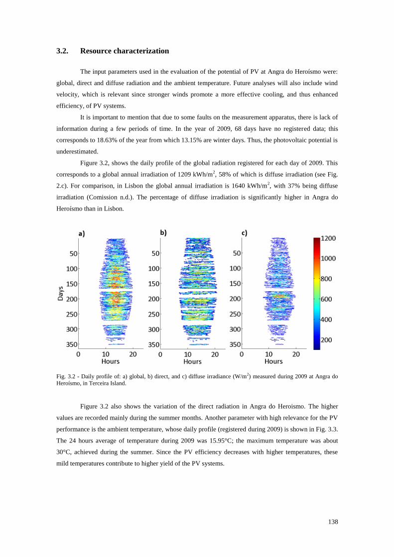
138

3.2. Resource characterization

The input parameters used in the evaluation of the potential of PV at Angra do Heroísmo were:

global, direct and diffuse radiation and the ambient temperature. Future analyses will also include wind

velocity, which is relevant since stronger winds promote a more effective cooling, and thus enhanced

efficiency, of PV systems.

It is important to mention that due to some faults on the measurement apparatus, there is lack of

information during a few periods of time. In the year of 2009, 68 days have no registered data; this

corresponds to 18.63% of the year from which 13.15% are winter days. Thus, the photovoltaic potential is

underestimated.

Figure 3.2, shows the daily profile of the global radiation registered for each day of 2009. This

corresponds to a global annual irradiation of 1209 kWh/m2, 58% of which is diffuse irradiation (see Fig.

2.c). For comparison, in Lisbon the global annual irradiation is 1640 kWh/m2, with 37% being diffuse

irradiation (Comission n.d.). The percentage of diffuse irradiation is significantly higher in Angra do

Heroísmo than in Lisbon.

Fig. 3.2 - Daily profile of: a) global, b) direct, and c) diffuse irradiance (W/m2) measured during 2009 at Angra do

Heroísmo, in Terceira Island.

Figure 3.2 also shows the variation of the direct radiation in Angra do Heroismo. The higher

values are recorded mainly during the summer months. Another parameter with high relevance for the PV

performance is the ambient temperature, whose daily profile (registered during 2009) is shown in Fig. 3.3.

The 24 hours average of temperature during 2009 was 15.95°C; the maximum temperature was about

30°C, achieved during the summer. Since the PV efficiency decreases with higher temperatures, these

mild temperatures contribute to higher yield of the PV systems.

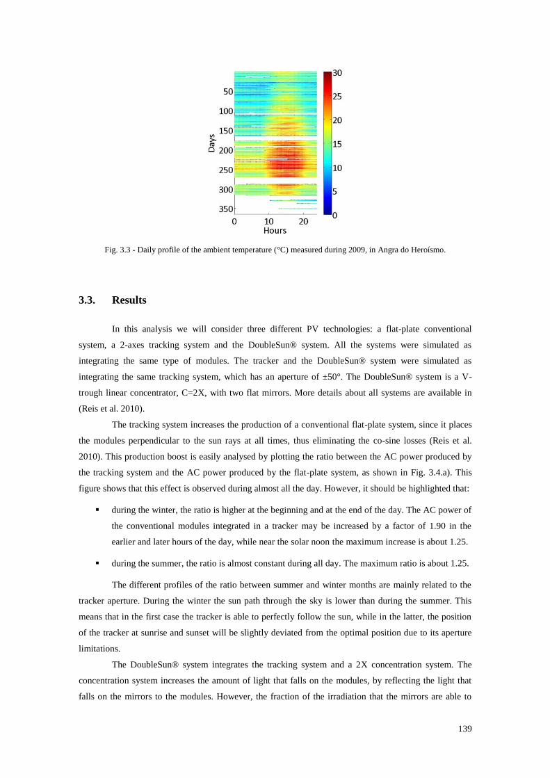
139

Fig. 3.3 - Daily profile of the ambient temperature (°C) measured during 2009, in Angra do Heroísmo.

3.3. Results

In this analysis we will consider three different PV technologies: a flat-plate conventional

system, a 2-axes tracking system and the DoubleSun® system. All the systems were simulated as

integrating the same type of modules. The tracker and the DoubleSun® system were simulated as

integrating the same tracking system, which has an aperture of ±50°. The DoubleSun® system is a V-

trough linear concentrator, C=2X, with two flat mirrors. More details about all systems are available in

(Reis et al. 2010).

The tracking system increases the production of a conventional flat-plate system, since it places

the modules perpendicular to the sun rays at all times, thus eliminating the co-sine losses (Reis et al.

2010). This production boost is easily analysed by plotting the ratio between the AC power produced by

the tracking system and the AC power produced by the flat-plate system, as shown in Fig. 3.4.a). This

figure shows that this effect is observed during almost all the day. However, it should be highlighted that:

during the winter, the ratio is higher at the beginning and at the end of the day. The AC power of

the conventional modules integrated in a tracker may be increased by a factor of 1.90 in the

earlier and later hours of the day, while near the solar noon the maximum increase is about 1.25.

during the summer, the ratio is almost constant during all day. The maximum ratio is about 1.25.

The different profiles of the ratio between summer and winter months are mainly related to the

tracker aperture. During the winter the sun path through the sky is lower than during the summer. This

means that in the first case the tracker is able to perfectly follow the sun, while in the latter, the position

of the tracker at sunrise and sunset will be slightly deviated from the optimal position due to its aperture

limitations.

The DoubleSun® system integrates the tracking system and a 2X concentration system. The

concentration system increases the amount of light that falls on the modules, by reflecting the light that

falls on the mirrors to the modules. However, the fraction of the irradiation that the mirrors are able to

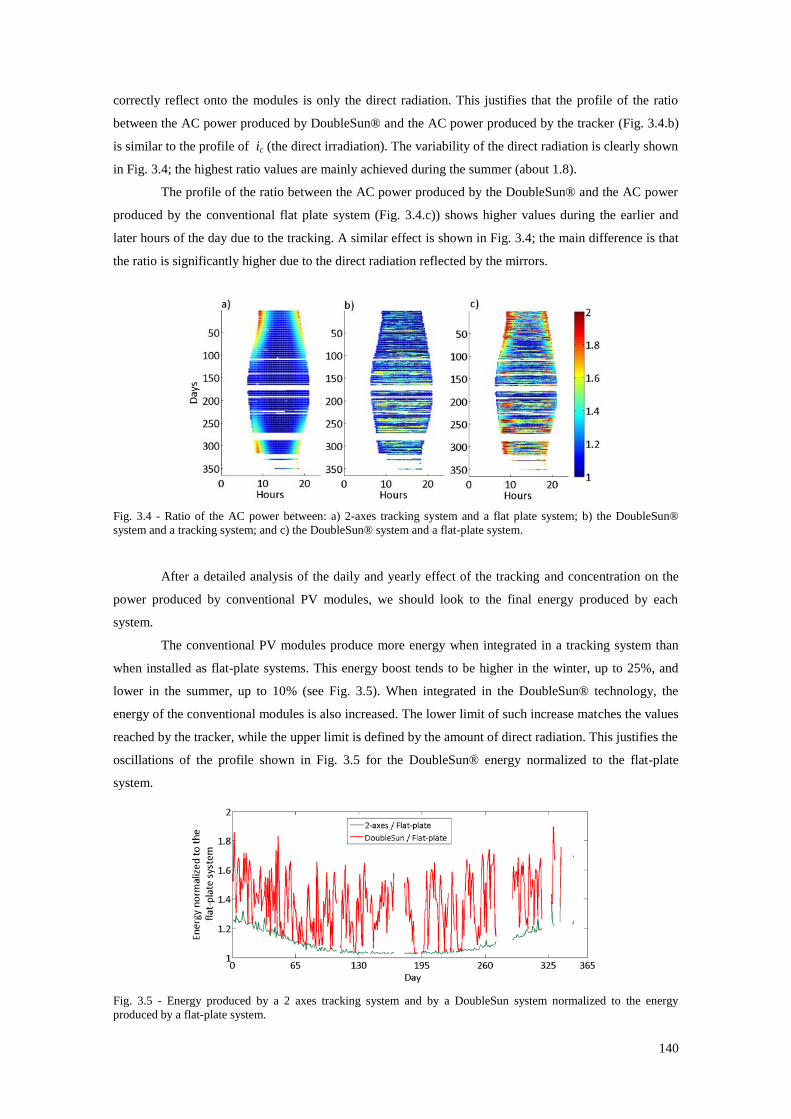
140

correctly reflect onto the modules is only the direct radiation. This justifies that the profile of the ratio

between the AC power produced by DoubleSun® and the AC power produced by the tracker (Fig. 3.4.b)

is similar to the profile of ic (the direct irradiation). The variability of the direct radiation is clearly shown

in Fig. 3.4; the highest ratio values are mainly achieved during the summer (about 1.8).

The profile of the ratio between the AC power produced by the DoubleSun® and the AC power

produced by the conventional flat plate system (Fig. 3.4.c)) shows higher values during the earlier and

later hours of the day due to the tracking. A similar effect is shown in Fig. 3.4; the main difference is that

the ratio is significantly higher due to the direct radiation reflected by the mirrors.

Fig. 3.4 - Ratio of the AC power between: a) 2-axes tracking system and a flat plate system; b) the DoubleSun®

system and a tracking system; and c) the DoubleSun® system and a flat-plate system.

After a detailed analysis of the daily and yearly effect of the tracking and concentration on the

power produced by conventional PV modules, we should look to the final energy produced by each

system.

The conventional PV modules produce more energy when integrated in a tracking system than

when installed as flat-plate systems. This energy boost tends to be higher in the winter, up to 25%, and

lower in the summer, up to 10% (see Fig. 3.5). When integrated in the DoubleSun® technology, the

energy of the conventional modules is also increased. The lower limit of such increase matches the values

reached by the tracker, while the upper limit is defined by the amount of direct radiation. This justifies the

oscillations of the profile shown in Fig. 3.5 for the DoubleSun® energy normalized to the flat-plate

system.

Fig. 3.5 - Energy produced by a 2 axes tracking system and by a DoubleSun system normalized to the energy

produced by a flat-plate system.

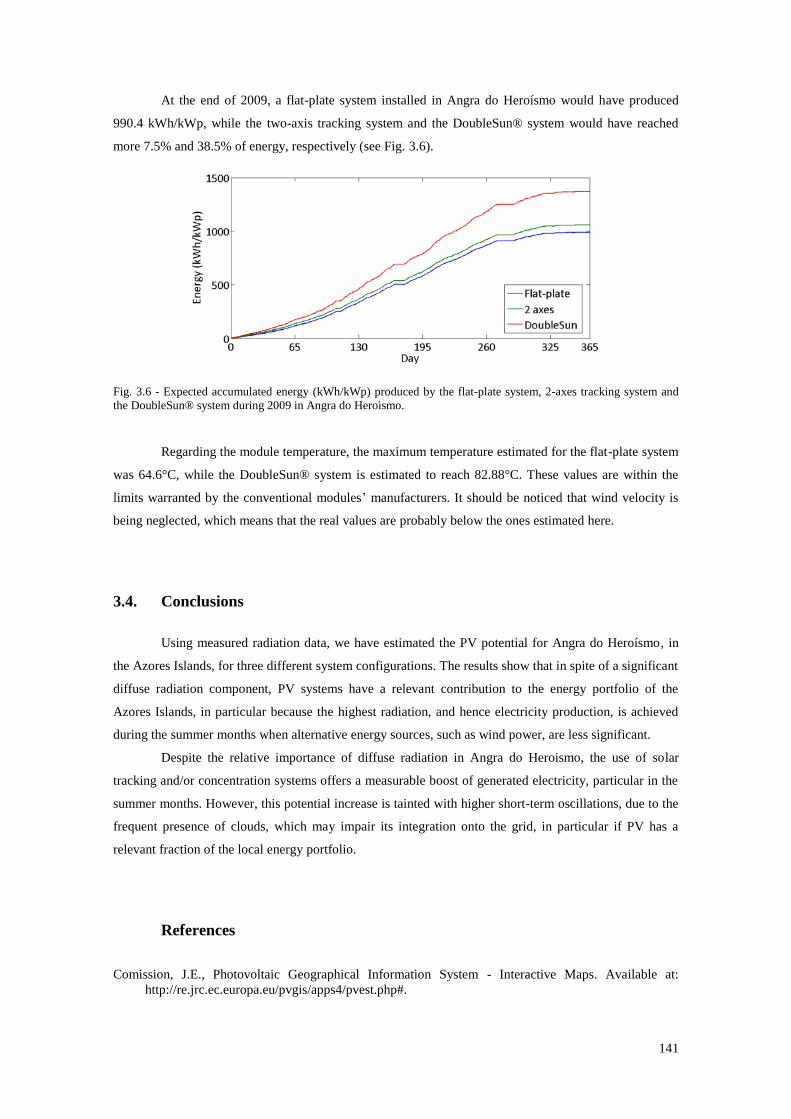
141

At the end of 2009, a flat-plate system installed in Angra do Heroísmo would have produced

990.4 kWh/kWp, while the two-axis tracking system and the DoubleSun® system would have reached

more 7.5% and 38.5% of energy, respectively (see Fig. 3.6).

Fig. 3.6 - Expected accumulated energy (kWh/kWp) produced by the flat-plate system, 2-axes tracking system and

the DoubleSun® system during 2009 in Angra do Heroismo.

Regarding the module temperature, the maximum temperature estimated for the flat-plate system

was 64.6°C, while the DoubleSun® system is estimated to reach 82.88°C. These values are within the

limits warranted by the conventional modules’ manufacturers. It should be noticed that wind velocity is

being neglected, which means that the real values are probably below the ones estimated here.

3.4. Conclusions

Using measured radiation data, we have estimated the PV potential for Angra do Heroísmo, in

the Azores Islands, for three different system configurations. The results show that in spite of a significant

diffuse radiation component, PV systems have a relevant contribution to the energy portfolio of the

Azores Islands, in particular because the highest radiation, and hence electricity production, is achieved

during the summer months when alternative energy sources, such as wind power, are less significant.

Despite the relative importance of diffuse radiation in Angra do Heroismo, the use of solar

tracking and/or concentration systems offers a measurable boost of generated electricity, particular in the

summer months. However, this potential increase is tainted with higher short-term oscillations, due to the

frequent presence of clouds, which may impair its integration onto the grid, in particular if PV has a

relevant fraction of the local energy portfolio.

References

Comission, J.E., Photovoltaic Geographical Information System - Interactive Maps. Available at:

http://re.jrc.ec.europa.eu/pvgis/apps4/pvest.php#.

142

Fans, C.L., Cruise Line Fans. Available at: http://www.cruiselinefans.com/other/6930-azores.html.

MITP, MIT Portugal - Sustainable Energy Systems. Available at:

http://www.mitportugal.org/sustainable-energy-systems/research-projects.html.

Reis, F. et al., 2010. Modeling the performance of low concentration photovoltaic systems. Solar Energy

Materials and Solar Cells, 94(7), pp.1222–1226. Available at:

http://linkinghub.elsevier.com/retrieve/pii/S0927024810001376 [Accessed January 31, 2012].

Reis, F. et al., 2011. Photovoltaic Potential in Terceira Island (Azores). In 26th European Photovoltaic

Solar Energy Conference and Exhibition. Hamburg, Germany.

Silva, B., 2010. Green Islands Azores. Available at: http://www.green-islands-azores.uac.pt/.

143

Chapter 4 Levelized cost of electricity

The purpose of the Levelized Cost of Electricity (LCoE) model described in this chapter is to

evaluate the different possible HSun options to achieve grid parity using photovoltaics. It corresponds to

the first step of the HSun project: defining the optimum concentration of a CPV system in order to

achieve the lowest possible electricity cost. The LCoE model compares different photovoltaic (PV)

systems configurations: conventional flat-plate, tracking system (one-axis and two-axis), and

concentrated photovoltaic (CPV) systems. The model assumptions as well as results are described in

detail in this chapter and in the paper (Reis et al. 2011) presented at the 26th

EUPVSEC.

4.1. Introduction

An accurate method to compare the cost of electricity across different technologies is the

Levelized Cost of Electricity (LCoE). This tool takes into account the net present value of the annual

energy, the capacity costs and annual costs during the system lifetime (Short et al. 1995; Nishikawa et al.

2008).

In this paper we present a LCoE model that was firstly developed to assess the current costs of

electricity for four different PV technologies that integrate standard crystalline silicon modules:

a conventional flat-plate system with optimal orientation and inclination;

a one-axis (East-West) tracking system;

a two-axis (both East-West and North-South) tracking system;

the DoubleSun® technology (Reis et al. 2010), a 2X concentration photovoltaic (CPV)

system.

The LCoE model was then adopted and used as an auxiliary design tool for the first decisions on

the development of the new CPV technology, the HSun (Mendes-Lopes et al. 2011).

4.2. LCoE model and assumptions

4.2.1. Capacity costs

The PV systems costs are only accounted in the installation year, year 0, and it consists of: i) the

cost of modules (CM); ii) costs of the so-called balance-of-system (BOS) which includes components such

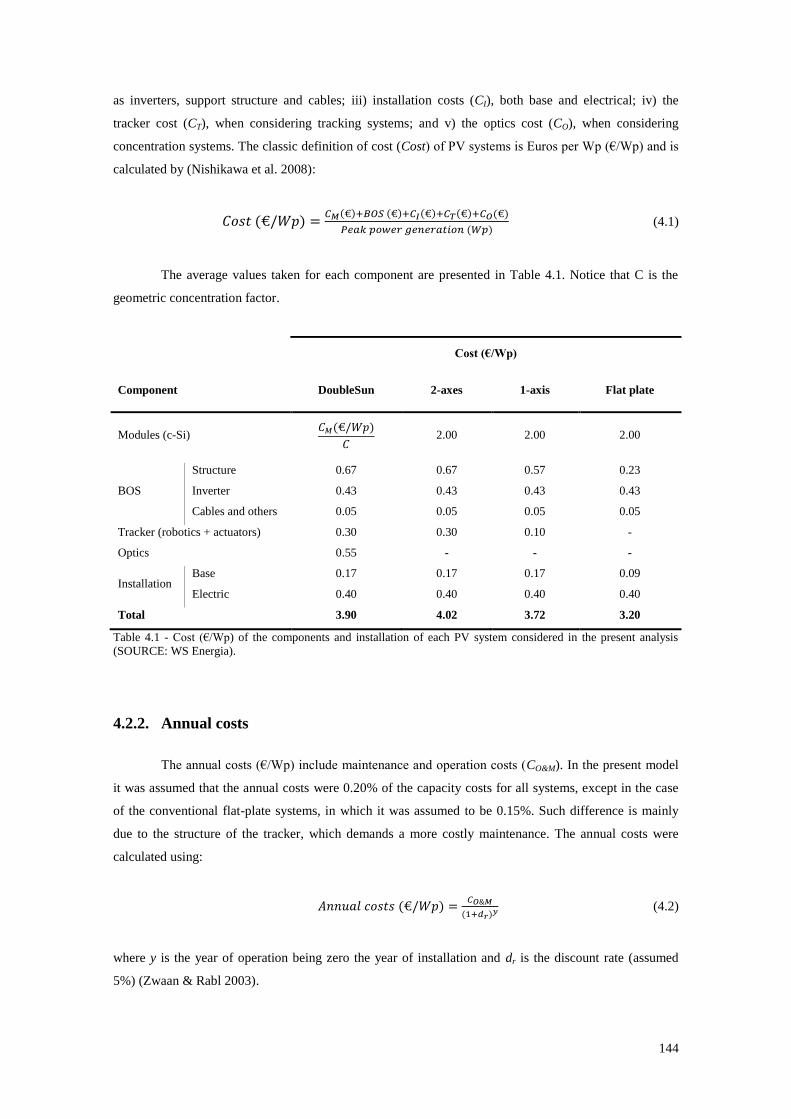
144

as inverters, support structure and cables; iii) installation costs (CI), both base and electrical; iv) the

tracker cost (CT), when considering tracking systems; and v) the optics cost (CO), when considering

concentration systems. The classic definition of cost (Cost) of PV systems is Euros per Wp (€/Wp) and is

calculated by (Nishikawa et al. 2008):

(4.1)

The average values taken for each component are presented in Table 4.1. Notice that C is the

geometric concentration factor.

Cost (€/Wp)

Component DoubleSun 2-axes 1-axis Flat plate

Modules (c-Si)

2.00 2.00 2.00

BOS

Structure 0.67 0.67 0.57 0.23

Inverter 0.43 0.43 0.43 0.43

Cables and others 0.05 0.05 0.05 0.05

Tracker (robotics + actuators) 0.30 0.30 0.10 -

Optics 0.55 - - -

Installation Base 0.17 0.17 0.17 0.09

Electric 0.40 0.40 0.40 0.40

Total 3.90 4.02 3.72 3.20

Table 4.1 - Cost (€/Wp) of the components and installation of each PV system considered in the present analysis

(SOURCE: WS Energia).

4.2.2. Annual costs

The annual costs (€/Wp) include maintenance and operation costs (CO&M). In the present model

it was assumed that the annual costs were 0.20% of the capacity costs for all systems, except in the case

of the conventional flat-plate systems, in which it was assumed to be 0.15%. Such difference is mainly

due to the structure of the tracker, which demands a more costly maintenance. The annual costs were

calculated using:

(4.2)

where y is the year of operation being zero the year of installation and dr is the discount rate (assumed

5%) (Zwaan & Rabl 2003).

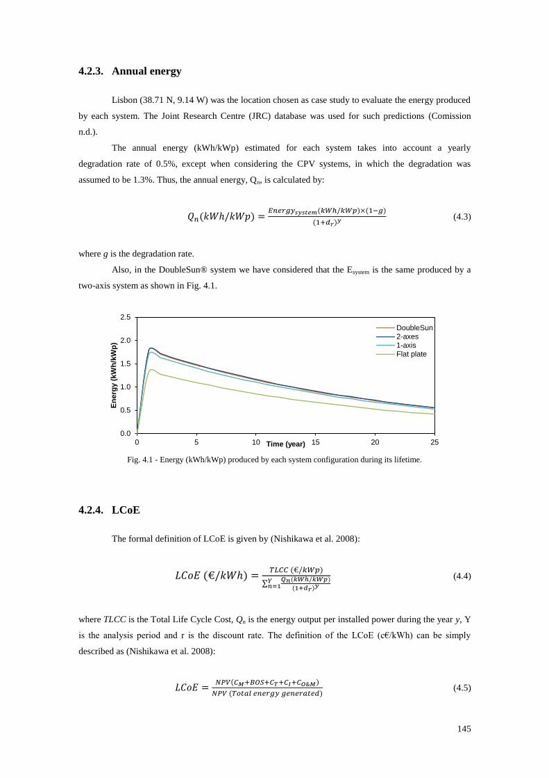
145

4.2.3. Annual energy

Lisbon (38.71 N, 9.14 W) was the location chosen as case study to evaluate the energy produced

by each system. The Joint Research Centre (JRC) database was used for such predictions (Comission

n.d.).

The annual energy (kWh/kWp) estimated for each system takes into account a yearly

degradation rate of 0.5%, except when considering the CPV systems, in which the degradation was

assumed to be 1.3%. Thus, the annual energy, Qn, is calculated by:

(4.3)

where g is the degradation rate.

Also, in the DoubleSun® system we have considered that the Esystem is the same produced by a

two-axis system as shown in Fig. 4.1.

Fig. 4.1 - Energy (kWh/kWp) produced by each system configuration during its lifetime.

4.2.4. LCoE

The formal definition of LCoE is given by (Nishikawa et al. 2008):

∑

(4.4)

where TLCC is the Total Life Cycle Cost, Qn is the energy output per installed power during the year y, Y

is the analysis period and r is the discount rate. The definition of the LCoE (c€/kWh) can be simply

described as (Nishikawa et al. 2008):

(4.5)

0.0

0.5

1.0

1.5

2.0

2.5

0 5 10 15 20 25

En

erg

y (

kW

h/k

Wp

)

Time (year)

DoubleSun

2-axes

1-axis

Flat plate

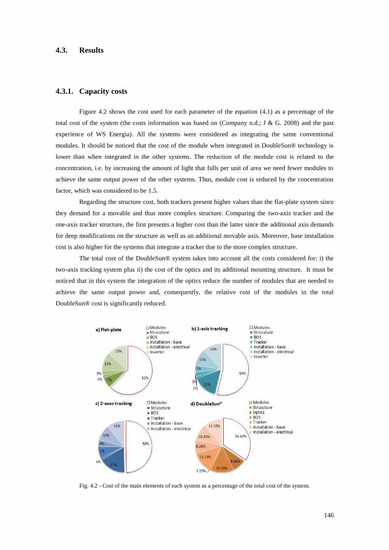
146

4.3. Results

4.3.1. Capacity costs

Figure 4.2 shows the cost used for each parameter of the equation (4.1) as a percentage of the

total cost of the system (the costs information was based on (Company n.d.; J & G. 2008) and the past

experience of WS Energia). All the systems were considered as integrating the same conventional

modules. It should be noticed that the cost of the module when integrated in DoubleSun® technology is

lower than when integrated in the other systems. The reduction of the module cost is related to the

concentration, i.e. by increasing the amount of light that falls per unit of area we need fewer modules to

achieve the same output power of the other systems. Thus, module cost is reduced by the concentration

factor, which was considered to be 1.5.

Regarding the structure cost, both trackers present higher values than the flat-plate system since

they demand for a movable and thus more complex structure. Comparing the two-axis tracker and the

one-axis tracker structure, the first presents a higher cost than the latter since the additional axis demands

for deep modifications on the structure as well as an additional movable axis. Moreover, base installation

cost is also higher for the systems that integrate a tracker due to the more complex structure.

The total cost of the DoubleSun® system takes into account all the costs considered for: i) the

two-axis tracking system plus ii) the cost of the optics and its additional mounting structure. It must be

noticed that in this system the integration of the optics reduce the number of modules that are needed to

achieve the same output power and, consequently, the relative cost of the modules in the total

DoubleSun® cost is significantly reduced.

Fig. 4.2 - Cost of the main elements of each system as a percentage of the total cost of the system.

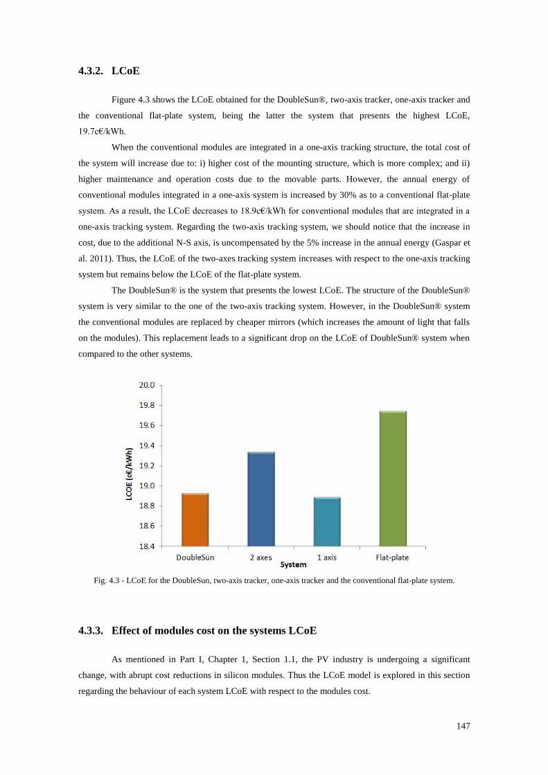
147

4.3.2. LCoE

Figure 4.3 shows the LCoE obtained for the DoubleSun®, two-axis tracker, one-axis tracker and

the conventional flat-plate system, being the latter the system that presents the highest LCoE,

19.7c€/kWh.

When the conventional modules are integrated in a one-axis tracking structure, the total cost of

the system will increase due to: i) higher cost of the mounting structure, which is more complex; and ii)

higher maintenance and operation costs due to the movable parts. However, the annual energy of

conventional modules integrated in a one-axis system is increased by 30% as to a conventional flat-plate

system. As a result, the LCoE decreases to 18.9c€/kWh for conventional modules that are integrated in a

one-axis tracking system. Regarding the two-axis tracking system, we should notice that the increase in

cost, due to the additional N-S axis, is uncompensated by the 5% increase in the annual energy (Gaspar et

al. 2011). Thus, the LCoE of the two-axes tracking system increases with respect to the one-axis tracking

system but remains below the LCoE of the flat-plate system.

The DoubleSun® is the system that presents the lowest LCoE. The structure of the DoubleSun®

system is very similar to the one of the two-axis tracking system. However, in the DoubleSun® system

the conventional modules are replaced by cheaper mirrors (which increases the amount of light that falls

on the modules). This replacement leads to a significant drop on the LCoE of DoubleSun® system when

compared to the other systems.

Fig. 4.3 - LCoE for the DoubleSun, two-axis tracker, one-axis tracker and the conventional flat-plate system.

4.3.3. Effect of modules cost on the systems LCoE

As mentioned in Part I, Chapter 1, Section 1.1, the PV industry is undergoing a significant

change, with abrupt cost reductions in silicon modules. Thus the LCoE model is explored in this section

regarding the behaviour of each system LCoE with respect to the modules cost.

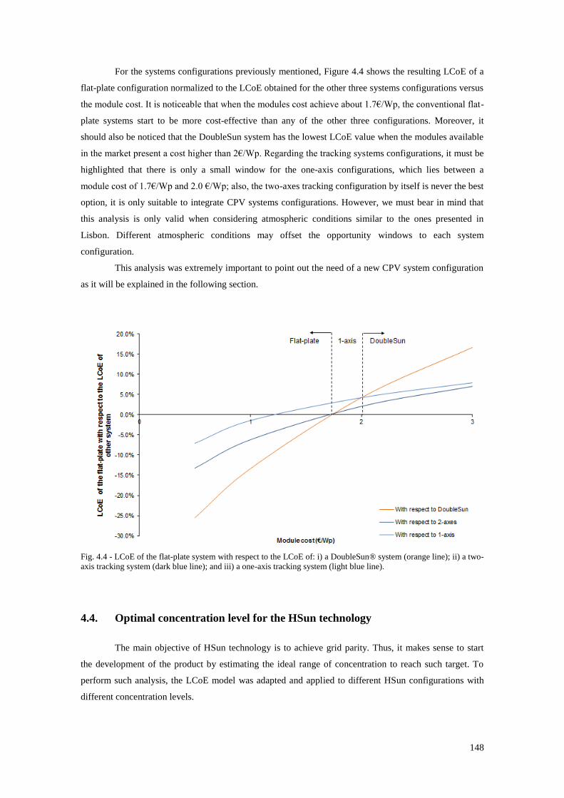
148

For the systems configurations previously mentioned, Figure 4.4 shows the resulting LCoE of a

flat-plate configuration normalized to the LCoE obtained for the other three systems configurations versus

the module cost. It is noticeable that when the modules cost achieve about 1.7€/Wp, the conventional flat-

plate systems start to be more cost-effective than any of the other three configurations. Moreover, it

should also be noticed that the DoubleSun system has the lowest LCoE value when the modules available

in the market present a cost higher than 2€/Wp. Regarding the tracking systems configurations, it must be

highlighted that there is only a small window for the one-axis configurations, which lies between a

module cost of 1.7€/Wp and 2.0 €/Wp; also, the two-axes tracking configuration by itself is never the best

option, it is only suitable to integrate CPV systems configurations. However, we must bear in mind that

this analysis is only valid when considering atmospheric conditions similar to the ones presented in

Lisbon. Different atmospheric conditions may offset the opportunity windows to each system

configuration.

This analysis was extremely important to point out the need of a new CPV system configuration

as it will be explained in the following section.

Fig. 4.4 - LCoE of the flat-plate system with respect to the LCoE of: i) a DoubleSun® system (orange line); ii) a two-

axis tracking system (dark blue line); and iii) a one-axis tracking system (light blue line).

4.4. Optimal concentration level for the HSun technology

The main objective of HSun technology is to achieve grid parity. Thus, it makes sense to start

the development of the product by estimating the ideal range of concentration to reach such target. To

perform such analysis, the LCoE model was adapted and applied to different HSun configurations with

different concentration levels.

149

4.4.1. Modifications on the LCoE model

First of all, we have to define the equation that predicts the power output of the HSun system for

different concentration levels. Hence, we begin by the definition of system efficiency ( ):

(4.6)

where, is the power of the system and is the irradiation that reaches the system, i.e.

1000W/m2, according to STC. Since we intend to estimate the system power, the previous equation must

be re-written as:

(4.7)

To estimate the system efficiency we first recall the definition of concentration, which is the

ratio between the primary optics and the active area of the system. On the other hand, bearing in mind that

the tracking system has a limited area, AT, for mounting of the PV modules, this area corresponds to the

maximum area available for the primary optics so that the active area ( ) of the system may be

defined by:

(4.8)

After defining the active area of the system, we must define the percentage of irradiation that

really falls on it. By taking the DoubleSun® as an example we should define two different origins for the

irradiation: i) concentrated sunlight (i.e. redirected by the primary optics to the active area) which is

affected by the optical efficiency ( and also the ratio between direct and total radiation (ic); and ii) un-

concentrated sunlight (i.e. radiation that reaches directly the active area without being scattered by other

CPV element). Following this assumptions, the efficiency of the radiation that reaches the active area is

given by:

(4.9)

On the other hand, the active area only converts part of the radiation that reaches its surface.

First, because the there are some gaps between the solar cells; and, second, because the solar cells have

efficiencies lower than 100%. This way we define the efficiency of the active area as εa and the efficiency

of the system should be given by:

( ) (4.10)

By replacing this equation in eq. (4.7) we may estimate the power of the system through:

( ) (4.11)

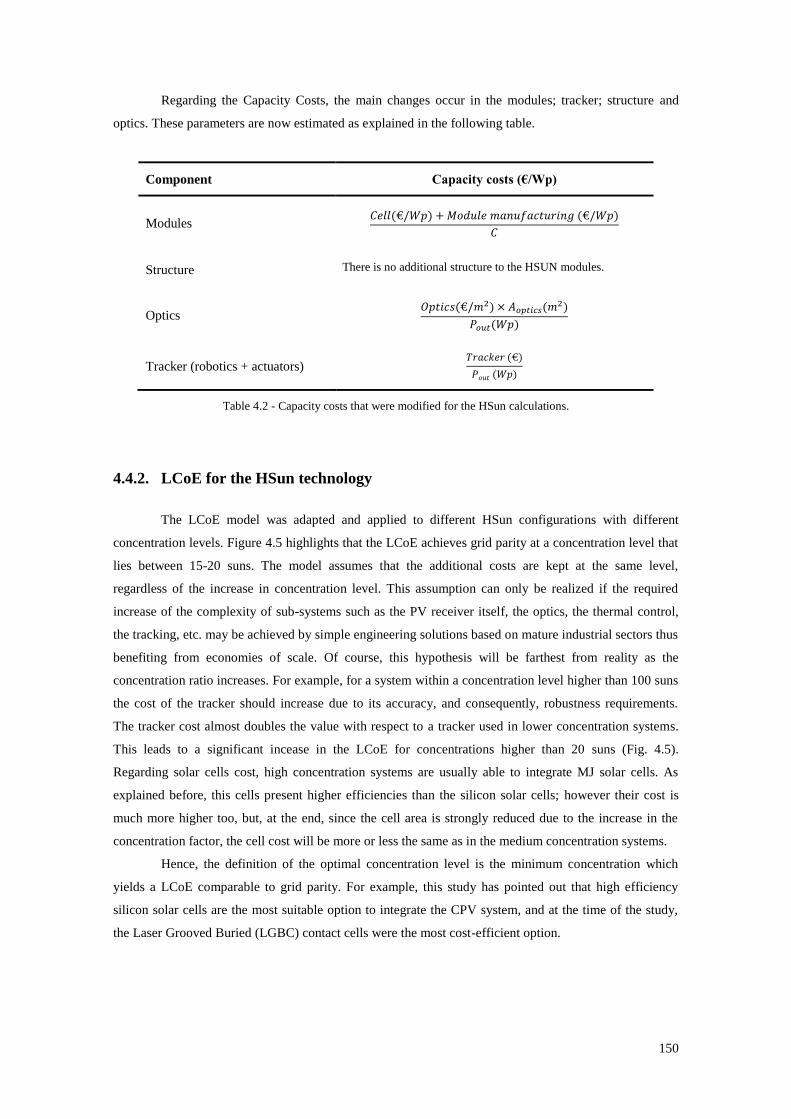
150

Regarding the Capacity Costs, the main changes occur in the modules; tracker; structure and

optics. These parameters are now estimated as explained in the following table.

Component Capacity costs (€/Wp)

Modules

Structure There is no additional structure to the HSUN modules.

Optics

Tracker (robotics + actuators)

Table 4.2 - Capacity costs that were modified for the HSun calculations.

4.4.2. LCoE for the HSun technology

The LCoE model was adapted and applied to different HSun configurations with different

concentration levels. Figure 4.5 highlights that the LCoE achieves grid parity at a concentration level that

lies between 15-20 suns. The model assumes that the additional costs are kept at the same level,

regardless of the increase in concentration level. This assumption can only be realized if the required

increase of the complexity of sub-systems such as the PV receiver itself, the optics, the thermal control,

the tracking, etc. may be achieved by simple engineering solutions based on mature industrial sectors thus

benefiting from economies of scale. Of course, this hypothesis will be farthest from reality as the

concentration ratio increases. For example, for a system within a concentration level higher than 100 suns

the cost of the tracker should increase due to its accuracy, and consequently, robustness requirements.

The tracker cost almost doubles the value with respect to a tracker used in lower concentration systems.

This leads to a significant incease in the LCoE for concentrations higher than 20 suns (Fig. 4.5).

Regarding solar cells cost, high concentration systems are usually able to integrate MJ solar cells. As

explained before, this cells present higher efficiencies than the silicon solar cells; however their cost is

much more higher too, but, at the end, since the cell area is strongly reduced due to the increase in the

concentration factor, the cell cost will be more or less the same as in the medium concentration systems.

Hence, the definition of the optimal concentration level is the minimum concentration which

yields a LCoE comparable to grid parity. For example, this study has pointed out that high efficiency

silicon solar cells are the most suitable option to integrate the CPV system, and at the time of the study,

the Laser Grooved Buried (LGBC) contact cells were the most cost-efficient option.

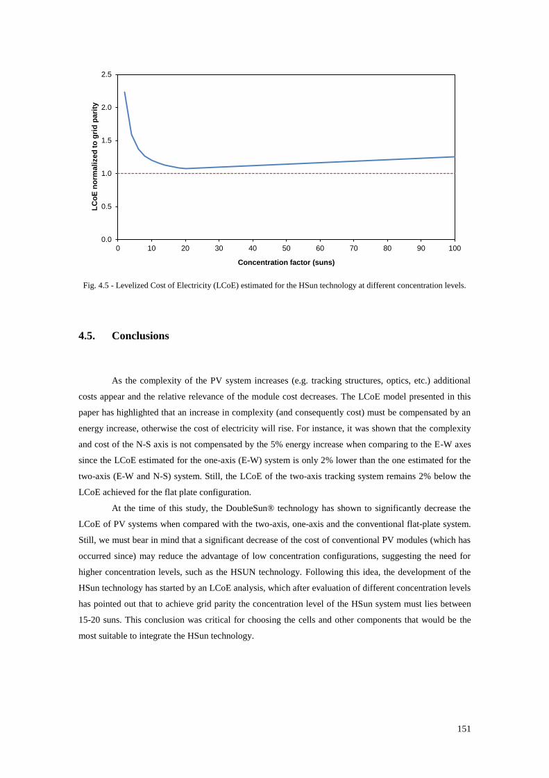
151

Fig. 4.5 - Levelized Cost of Electricity (LCoE) estimated for the HSun technology at different concentration levels.

4.5. Conclusions

As the complexity of the PV system increases (e.g. tracking structures, optics, etc.) additional

costs appear and the relative relevance of the module cost decreases. The LCoE model presented in this

paper has highlighted that an increase in complexity (and consequently cost) must be compensated by an

energy increase, otherwise the cost of electricity will rise. For instance, it was shown that the complexity

and cost of the N-S axis is not compensated by the 5% energy increase when comparing to the E-W axes

since the LCoE estimated for the one-axis (E-W) system is only 2% lower than the one estimated for the

two-axis (E-W and N-S) system. Still, the LCoE of the two-axis tracking system remains 2% below the

LCoE achieved for the flat plate configuration.

At the time of this study, the DoubleSun® technology has shown to significantly decrease the

LCoE of PV systems when compared with the two-axis, one-axis and the conventional flat-plate system.

Still, we must bear in mind that a significant decrease of the cost of conventional PV modules (which has

occurred since) may reduce the advantage of low concentration configurations, suggesting the need for

higher concentration levels, such as the HSUN technology. Following this idea, the development of the

HSun technology has started by an LCoE analysis, which after evaluation of different concentration levels

has pointed out that to achieve grid parity the concentration level of the HSun system must lies between

15-20 suns. This conclusion was critical for choosing the cells and other components that would be the

most suitable to integrate the HSun technology.

0.0

0.5

1.0

1.5

2.0

2.5

0 10 20 30 40 50 60 70 80 90 100

LC

oE

no

rma

lize

d t

o g

rid

pa

rity

Concentration factor (suns)

152

References

Comission, J.E., Photovoltaic Geographical Information System - Interactive Maps. Available at:

http://re.jrc.ec.europa.eu/pvgis/apps4/pvest.php#.

Company, N.G., Solarbuzz - Solar Market Research and Analysis. Available at:

http://www.solarbuzz.com/facts-and-figures/retail-price-environment/module-prices.

Gaspar, G. et al., 2011. Exploring One-Axis Tracking Configurations For CPV Application. In 7th

International Conference on Concentrating Photovoltaic Systems: CPV-7. AIP Conference

Proceedings.

J, S. & G., H., 2008. Gearing up for a price war. In: The market for tracking systems is entering a new

phase: that of uncompromising optimization. Photon International;

Mendes-Lopes, J. et al., 2011. On-field Demonstration Results of Medium Concentration System

HSUN®. In CPV-7 conference. Las Vegas, USA.

Nishikawa, W., Horne, S. & Ave, L., 2008. Key advantages of Concentrating Photovoltaics (CPV) for

Lowering Levelized Cost Of Electricity (LCOE). In 23rd European Photovoltaic Solar Energy

Conference. Valencia, Spain. Available at:

http://www.solfocus.com/en/downloads/news/2008.0901_EUPVSEC_CPV-

LCOE_WNishikawa.pdf.

Reis, F. et al., 2011. LCoE Analysis as a Decision Tool for Design of Concentrated Photovoltaic Systems.

In 26th European Photovoltaic Solar Energy Conference and Exhibition. Hamburg, Germany, pp.

4581 – 4583. Available at: http://www.eupvsec-proceedings.com/proceedings?paper=10131.

Reis, F. et al., 2010. Modeling the performance of low concentration photovoltaic systems. Solar Energy

Materials and Solar Cells, 94(7), pp.1222–1226. Available at:

http://linkinghub.elsevier.com/retrieve/pii/S0927024810001376 [Accessed January 31, 2012].

Short, W., Packey, D.J. & Holt, T., 1995. A Manual for the Economic Evaluation of Energy Efficiency

and Renewable Energy Technologies, Colorado. Available at:

http://large.stanford.edu/publications/coal/references/troughnet/market/docs/5173.pdf.

Zwaan, B. Van Der & Rabl, A., 2003. Prospects for PV: a learning curve analysis. Solar Energy, 74,

pp.19–31. Available at: http://dx.doi.org/10.1016/S0038-092X(03)00112-9.

153

Conclusions

Concentration Photovoltaic (CPV) is a concept that appeared as an attempt to significantly

reduce the cost of Photovoltaic (PV) systems. Conceptually, the savings in the systems are achieved by

the reduction in PV cell area accompanied by the corresponding increase in the light intensity on the

device through optical devices (less expensive) that redirect the sunlight onto the solar cells (more

expensive). The history of CPV was briefly reviewed in Chapter 1 and the terms/concepts/definitions

used in this field were described in detail. Also in that chapter, the CPV components were classified and a

quantitative analysis of the options that have been carried out in CPV history has led to the conclusion

that the majority of the CPV systems developed so far may be classified as High Concentration

Photovoltaic (HCPV) solutions, with more than 44% of the systems analysed in this study presenting a

concentration factor above 400 suns. Hereupon, and since there is a compromise between each CPV

component, the refractive point-focus is the prevalent option for the optics, representing about 19% of the

systems under study, while the most common choice for solar cells, with about 38% of the systems, are

multijunction solar cells technology. As expected, 60% of the CPV systems integrate a tracking system,

from which 57% correspond to dual-axis systems.

Between 2007 and 2008, many LCPV concepts were developed. At that time silicon modules

were extremely expensive and many companies designed ingenious methods for making their

conventional silicon modules generate more electricity such as the solution developed by WS Energia

S.A. with the DoubleSun® technology, discussed in detail in Part II, Chapters 1, 2 and 3. However, the

sharp fall in the price of the modules lead to decreasing interest in this approach.

In this context, a Levelized Cost of Electricity (LCoE) analysis has shown that the optimum

concentration level to achieve grid parity should lie between 15 – 20 suns and high efficiency silicon cells

should be used. This study, which is presented in detail in Part II, Chapter 4, was used as a design tool for

the HSun technology, a medium CPV system that was developed by WS Energia S.A. The tool has

established boundaries on the options that have to be taken for the system design and development, which

are driven by the technological degree of development, efficiency, reliability and expected scalability of

the different system components. Further work regarding LCoE analysis may be performed in order to

update the data and find new paths for CPV applications.

Regarding the development of the HSun system, this work focused on the PV receiver, whose

components and development phases, as well as validation of the resulting prototypes were thoroughly

addressed in Chapter 2. Two main high efficiency silicon solar cells were identified as the most suitable

to integrate the technology under study: i) the Laser Grooved Buried Contact (LGBC) and ii) the

upgraded screen-printed solar cells. Both technologies are fully characterized in terms of electrical and

thermal parameters. Comparing both cells regarding cost/efficiency, in the long-term, LGBC solar cells

are likely to achieve a better cost-efficiency relation than upgraded screen-printed solar cells.

Nevertheless, at this stage of development, the Solartec cells featured a higher efficiency/cost ratio.

Hence, we decided to develop the PV receiver considering both cells. Additionally to the solar cells, the

154

PV receiver development has relied on: i) development of interconnection methods (soldering process) to

electrically connect the solar cells; ii) design of the board where the cells are placed; and iii) integration

of the bypass diodes. A first prototype was constructed and tested thus leading to a second prototype,

which was again optimized to build a final PV receiver which was validated.

Once the final prototype was defined, we proceeded to the analysis of its thermal behaviour

Chapter 3. First, we have experimentally measured the thermal resistances between the layers that

compose the PV receiver. It was noticed that the thermal resistance between the cell and the copper grid

layer (which corresponds to the printed circuit on the PV receiver board) was appreciably higher than the

thermal resistance between the copper layer and the aluminium layer (being the latter the material that

corresponds to the PV receiver base) thus suggesting that it may be an opportunity for further

improvement of the thermal contact. The experimental setup was then reproduced in the CFD-FEA

simulation using SolidWorks. The obtained results strongly match the experimental data thus allowing the

use of the model for evaluation of the temperature distribution across the cell. This analysis highlighted

that the areas near the soldering points were cooler than elsewhere on the solar cell. Thus, the electrical

interconnection strongly affects the distribution of the temperature on the cell which, consequently,

influences the efficiency of the cell. A final thermal study was then carried out for the complete PV

receiver (i.e. including the silicon layer, glass and secondary optics) when integrated in the HSun system.

The illumination profile was considered to be inhomogeneous (similar to a Gaussian profile with an

average value of 18 suns) and the resulting temperature distribution on the receiver and cells was

analysed. We came to the conclusion that i) the primary optics play an important role on the receiver

cooling since it may decrease the solar cells temperature by about 60°C; ii) the solar cells on the receiver

reach different average temperatures which may put some constraints on the PV receiver efficiency; and

iii) each solar cell feature an inhomogeneous distribution of temperature. This latter point has highlighted

the need for careful analysis of the effect of the temperature profile on the performance of the solar cells

thus demanding for the development of a solar cell electric model.

As mentioned above, an electric solar cell model was built to study the effect of inhomogeneous

temperature distribution across a solar cell; it also addresses the effect of an inhomogeneous illumination

profile on the cells performance, as discussed below. This model is described in detail in Chapter 4;

additionally, a detailed literature review of the distributed diode effect modelling is performed. In Chapter

5 the implementation of the distributed model is described, without loss of generality, for the LGBC solar

cell under study. This cell was fully characterized in terms of series resistance components whose value is

one of the critical inputs of the model.

The distributed model results are compared with the standard lumped model of a solar cell which

carelessly describes the behaviour of a solar cell working under concentrated irradiation and

inhomogeneous profiles of illumination and temperature. For the case study presented under

homogeneous illumination and temperature conditions, at 30 suns and 25°C, respectively, the standard

lumped model features a maximum power point 29% below the Pmp of the distributed model. This

difference showed that, under concentrated irradiation, the lumped model overestimates the resistive

losses that occur on a solar cell since it considers that the total current generated on the cell passes

through a single lumped series resistance instead of, as modelled in a distributed approach, crossing a

155

path with different series resistance components that depend on the region where the current is generated.

Thus, for an accurate estimation of the solar cell behaviour under inhomogeneous conditions of

illumination and temperature, the model presented in Chapter 4 consists in a distributed diode model in

which the cell is divided into small units whose electric circuit lies on a diode in parallel with a shunt

resistor and a series resistor component which depends on the region of the cell where the unit is located.

The model was built in Matlab/Simulink environment as explained in detail in Chapter 4.

Model validation was then thoroughly addressed in Chapter 6 for a set of inhomogeneous

illumination and temperature profiles in a temperature range of 25°C up to 70°C and concentration levels

from 1 sun up to 30 suns. For each case, I-V curves were measured and compared against model results

showing good agreement; nevertheless, the profile of inhomogeneous temperature distribution whose

minimum temperature is at the busbar seems to need further refinement on the model. For this particular

case, a maximum deviation of 2% on the Voc was found between experimental and modelled results. For

all other validation tests the deviation between model and experimental data was shown to be below

0.75%.

The distributed model was explored in Chapter 7, where a set of case studies with different

illumination and temperature profiles are compared regarding their impact on the solar cell’s

performance. To describe the inhomogeneity of the illumination and temperature on the solar cell, the

inhomogeneity parameters r and t were defined. It was shown that:

• for the same average irradiation, sharper illumination profiles (higher r) increase the power

losses. This effect may reach 7.5% for the cases whose maximum peak illumination is far

from the busbar and 6% when the maximum peak illumination is near the busbar;

• for different temperature profiles, it was observed that increasing temperature

inhomogeneity leads to lower voltages. In the case study analysed, a 22% decrease in Voc

was found for a temperature distribution whose maximum peak temperature is near the

busbar with respect to the STC case.

Additionally, in Chapter 7, we have also analysed the effect of the temperature and illumination

that are exhibited by the HSun technology. Depending of the cell location on the PV receiver, the solar

cells’ efficiency is about 12.6%. An optimization of the front fingers contact design has shown that this

efficiency may be improved by +1.5% (relative) if the cell was designed with 129 fingers instead of 108.

A decrease in the solar cells’ temperature would also lead to a significantly improvement on its

efficiency.

As far as future work is concerned, it is clear that it would be interesting to test the PV receiver

estimated performance with real data provided by a final prototype of the HSun technology. Furthermore,

and as mentioned above, the challenge faced for the particular case of temperature profiles whose

minimum temperature is at the busbar should be addressed. Different approaches, including 2D

modelling, more elementary units, or considering higher recombination under the busbar, have already

been unsuccessfully tested and therefore it is not clear the source of the mismatch. It might be related to

non-linear physical effects on the dark diode under the busbar, and therefore further experimental

characterization at the microscope level would probably be required to tackle this issue.

156

Other interesting open doors for future work regard the application of the distributed model to

other solar cell technologies such as back contact solar cells and multi-junction solar cells. The modelling

of these alternative concepts would require adding further components to the model electric circuit and

careful experimental characterization, but would certainly find relevant applications and interest.

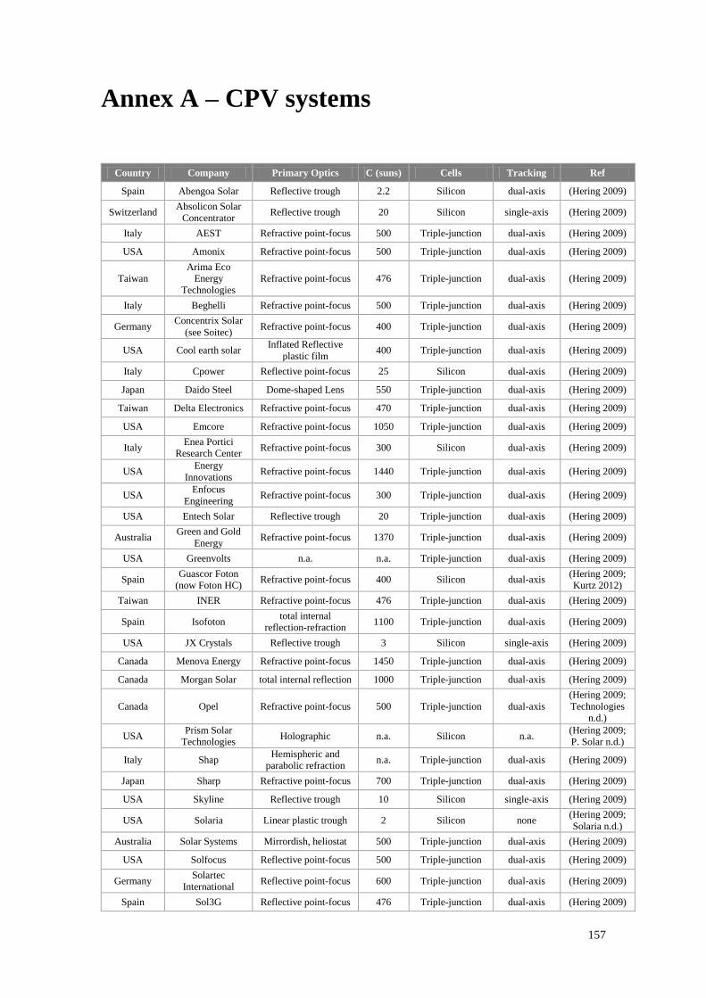
157

Annex A – CPV systems

Country Company Primary Optics C (suns) Cells Tracking Ref

Spain Abengoa Solar Reflective trough 2.2 Silicon dual-axis (Hering 2009)

Switzerland Absolicon Solar

Concentrator Reflective trough 20 Silicon single-axis (Hering 2009)

Italy AEST Refractive point-focus 500 Triple-junction dual-axis (Hering 2009)

USA Amonix Refractive point-focus 500 Triple-junction dual-axis (Hering 2009)

Taiwan

Arima Eco

Energy

Technologies

Refractive point-focus 476 Triple-junction dual-axis (Hering 2009)

Italy Beghelli Refractive point-focus 500 Triple-junction dual-axis (Hering 2009)

Germany Concentrix Solar

(see Soitec) Refractive point-focus 400 Triple-junction dual-axis (Hering 2009)

USA Cool earth solar Inflated Reflective

plastic film 400 Triple-junction dual-axis (Hering 2009)

Italy Cpower Reflective point-focus 25 Silicon dual-axis (Hering 2009)

Japan Daido Steel Dome-shaped Lens 550 Triple-junction dual-axis (Hering 2009)

Taiwan Delta Electronics Refractive point-focus 470 Triple-junction dual-axis (Hering 2009)

USA Emcore Refractive point-focus 1050 Triple-junction dual-axis (Hering 2009)

Italy Enea Portici

Research Center Refractive point-focus 300 Silicon dual-axis (Hering 2009)

USA Energy

Innovations Refractive point-focus 1440 Triple-junction dual-axis (Hering 2009)

USA Enfocus

Engineering Refractive point-focus 300 Triple-junction dual-axis (Hering 2009)

USA Entech Solar Reflective trough 20 Triple-junction dual-axis (Hering 2009)

Australia Green and Gold

Energy Refractive point-focus 1370 Triple-junction dual-axis (Hering 2009)

USA Greenvolts n.a. n.a. Triple-junction dual-axis (Hering 2009)

Spain Guascor Foton

(now Foton HC) Refractive point-focus 400 Silicon dual-axis

(Hering 2009;

Kurtz 2012)

Taiwan INER Refractive point-focus 476 Triple-junction dual-axis (Hering 2009)

Spain Isofoton total internal

reflection-refraction 1100 Triple-junction dual-axis (Hering 2009)

USA JX Crystals Reflective trough 3 Silicon single-axis (Hering 2009)

Canada Menova Energy Refractive point-focus 1450 Triple-junction dual-axis (Hering 2009)

Canada Morgan Solar total internal reflection 1000 Triple-junction dual-axis (Hering 2009)

Canada Opel Refractive point-focus 500 Triple-junction dual-axis

(Hering 2009;

Technologies

n.d.)

USA Prism Solar

Technologies Holographic n.a. Silicon n.a.

(Hering 2009;

P. Solar n.d.)

Italy Shap Hemispheric and

parabolic refraction n.a. Triple-junction dual-axis (Hering 2009)

Japan Sharp Refractive point-focus 700 Triple-junction dual-axis (Hering 2009)

USA Skyline Reflective trough 10 Silicon single-axis (Hering 2009)

USA Solaria Linear plastic trough 2 Silicon none (Hering 2009;

Solaria n.d.)

Australia Solar Systems Mirrordish, heliostat 500 Triple-junction dual-axis (Hering 2009)

USA Solfocus Reflective point-focus 500 Triple-junction dual-axis (Hering 2009)

Germany Solartec

International Reflective point-focus 600 Triple-junction dual-axis (Hering 2009)

Spain Sol3G Reflective point-focus 476 Triple-junction dual-axis (Hering 2009)

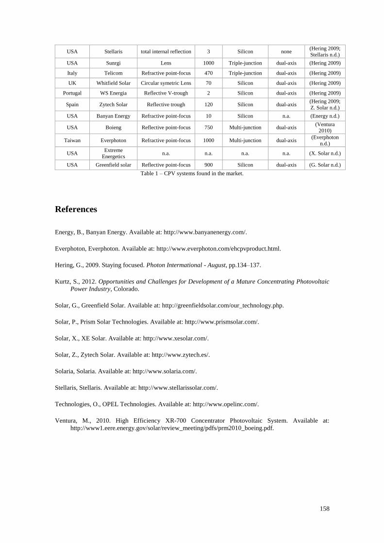
158

USA Stellaris total internal reflection 3 Silicon none (Hering 2009;

Stellaris n.d.)

USA Sunrgi Lens 1000 Triple-junction dual-axis (Hering 2009)

Italy Telicom Refractive point-focus 470 Triple-junction dual-axis (Hering 2009)

UK Whitfield Solar Circular symetric Lens 70 Silicon dual-axis (Hering 2009)

Portugal WS Energia Reflective V-trough 2 Silicon dual-axis (Hering 2009)

Spain Zytech Solar Reflective trough 120 Silicon dual-axis (Hering 2009;

Z. Solar n.d.)

USA Banyan Energy Refractive point-focus 10 Silicon n.a. (Energy n.d.)

USA Boieng Reflective point-focus 750 Multi-junction dual-axis (Ventura

2010)

Taiwan Everphoton Refractive point-focus 1000 Multi-junction dual-axis (Everphoton

n.d.)

USA Extreme

Energetics n.a. n.a. n.a. n.a. (X. Solar n.d.)

USA Greenfield solar Reflective point-focus 900 Silicon dual-axis (G. Solar n.d.)

Table 1 – CPV systems found in the market.

References

Energy, B., Banyan Energy. Available at: http://www.banyanenergy.com/.

Everphoton, Everphoton. Available at: http://www.everphoton.com/ehcpvproduct.html.

Hering, G., 2009. Staying focused. Photon Intermational - August, pp.134–137.

Kurtz, S., 2012. Opportunities and Challenges for Development of a Mature Concentrating Photovoltaic

Power Industry, Colorado.

Solar, G., Greenfield Solar. Available at: http://greenfieldsolar.com/our_technology.php.

Solar, P., Prism Solar Technologies. Available at: http://www.prismsolar.com/.

Solar, X., XE Solar. Available at: http://www.xesolar.com/.

Solar, Z., Zytech Solar. Available at: http://www.zytech.es/.

Solaria, Solaria. Available at: http://www.solaria.com/.

Stellaris, Stellaris. Available at: http://www.stellarissolar.com/.

Technologies, O., OPEL Technologies. Available at: http://www.opelinc.com/.

Ventura, M., 2010. High Efficiency XR-700 Concentrator Photovoltaic System. Available at:

http://www1.eere.energy.gov/solar/review_meeting/pdfs/prm2010_boeing.pdf.