Development of high -resolution multi -scale m odelling … urban... · In this context , the authors present in this paper for the first time the application of the state-of-the

1

Development of high-resolution multi-scale modelling system 1

for simulation of coastal-fluvial urban flooding 2

Agnieszka Indiana Olbert1, Joanne Comer1, Stephen Nash1, Michael Hartnett1 3

1Civil Engineering, College of Engineering and Informatics, Ryan Institute, National University of Ireland, 4

Galway, University Road, Galway, Ireland 5

Correspondence to: Dr. Agnieszka Indiana Olbert ([email protected]) 6

7

Abstract. Urban developments in coastal zones are often exposed to natural hazards such as flooding. In this 8

research, a state-of-the-art, multi-scale nested flood (MSN_Flood) model is applied to simulate complex coastal-9

fluvial urban flooding due to combined effects of tides, surges and river discharges. Cork City on Ireland’s 10

southwest coast is a study case. The flood modelling system comprises of a cascade of four dynamically linked 11

models that resolve the hydrodynamics of Cork Harbour and/or its sub region at four scales 90m, 30m, 6m and 12

2m. 13

Results demonstrate that the internalisation of the nested boundary through a use of ghost cells combined with a 14

tailored adaptive interpolation technique creates a highly dynamic moving boundary that permits flooding and 15

drying of the nested boundary. This novel feature of MSN_Flood provides a high degree of choice regarding the 16

location of the boundaries to the nested domain and therefore flexibility in model application. The nested 17

MSN_Flood model through dynamic downscaling facilitates significant improvements in accuracy of model 18

output without incurring the computational expense of high spatial resolution over the entire model domain. The 19

urban flood model provides full characteristics of water levels and flow regimes necessary for flood hazard 20

identification and flood risk assessment. 21

22

23

Keywords: Urban flooding; Coastal flooding; Fluvial flooding; Hydrodynamic modelling; Nesting; Moving 24

boundary 25

26

27

28

Nat. Hazards Earth Syst. Sci. Discuss., doi:10.5194/nhess-2016-238, 2016Manuscript under review for journal Nat. Hazards Earth Syst. Sci.Published: 18 July 2016c© Author(s) 2016. CC-BY 3.0 License.

2

1 Introduction 29

Low lying developments in coastal zones are exposed to natural hazards such as storm surges, waves, tsunamis 30

and/or high river flows which can lead to significant flooding. Coastal flooding can result in substantial 31

economic and social impacts including loss of life, damage to property and disruption of essential services 32

(Brown et al. 2007). 33

Coastal flooding results from a rise of sea water level above normal predicted tide level. On the European 34

Continental Shelf, coastal flooding is associated with storms generated in the Atlantic Ocean that travel through, 35

or in proximity to, the shelf. Storm surges are important consequences of these storms – a temporary water setup 36

resulting from synoptic variation of atmospheric pressure and strong winds blowing towards the shelf causing 37

water to pile up against the coast. Surge physics is well understood in principle (Ponte, 1994); the mechanism of 38

its propagation on the European continental shelf as a response to meteorological conditions (wind stress and 39

atmospheric pressure signal separate) has been explained by Olbert and Hartnett (2010). 40

Flood dynamics due to a combination of multiple process drivers such as tides, surges and river inflows and 41

their interactions is extremely difficult to understand using non-modelling methods (Robins et al, 2011). In 42

recent years the amount of flood modelling work has risen dramatically. Yet the modelling still encounters 43

various problems of which input data such as topography (Mason et al, 2007; Smith, 2002), mesh resolution 44

(Sanders et al, 2010; Fewtrell, 2011; Horritt et al, 2006; Yu and Lane, 2006), bottom roughness (Mason et al., 45

2003; Horritt, 2000) or modelling framework (Hunter et al., 2008) are of greatest challenge. So far, one of the 46

main issues hampering research into coastal flood modelling has been the lack of topographic data of 47

sufficiently high resolution and accuracy along with highly resolvable efficient models. In the past decade, high 48

resolution topographic has become more available with airborne scanning laser altimetry (LIDAR) technology 49

(Gomes-Pereira and Wicherson, 1999) providing high resolution digital surface maps that can be used as model 50

bathymetry (Marks and Bates, 2000). Although there are still problems with mapping urban areas and 51

considerable post-processing is necessary to extract digital terrain model from digital surface model (Mason at 52

al., 2007), the hydraulic/hydrodynamic models developed using LIDAR data allow them to numerically 53

propagate surge and tidal waves into coastal areas. Model accuracy and computational cost are still issues to be 54

addressed. 55

The most common and simple approach to the modelling of coastal flooding in urban areas is to link (externally 56

or dynamically) longitudinal 1D or latterly averaged 2D hydraulic models with coastal models (e.g. Formaggia, 57

2001; Chen, 2007; Brown et al., 2007). Such a set up has two significant drawbacks. Firstly, 1D/2D hydraulic 58


3

models work with the assumption that the lateral variations in velocity magnitudes are small, while in reality 59

many coastal floodplains (e.g. urban areas) contain channels that have a significant influence on the 60

development of inundation by providing routes along which storm surges propagate inland (Bates et al., 2005) 61

and therefore may lead to misrepresentation of localized flooding (Cook and Merwade, 2009; Mark et al, 2004). 62

Secondly, numerical errors may be introduced when linking different models with different dimensions resulting 63

from poor conservation of momentum (Yang et al., 2012). There is evidence of proven difficulty in ensuring 64

that each model interprets the model inputs and boundary conditions in the same way (Hunter et al. 2008; 65

Pender and Neelz, 2010). 66

These problems may be overcome by application of a single hydrodynamic model to both coastal waters and 67

coastal floodplains. Although such a model would allow smooth transition of the model solution between 68

coastal waters and floodplains, the full solution at scales appropriate for flood inundation would incur a 69

significant computational cost. On one hand, such models need to extend far enough offshore to capture the 70

development and propagation of surge and to resolve the nonlinear shallow water dynamics (interactions 71

between tides, surges and waves) at a resolution that is commensurate with flow features. On the other hand the 72

model needs to include upstream river channels, tidal flats, low-lying land and urban areas which are susceptible 73

to flooding at very fine resolution. This often results in a model setup that requires a large computational domain 74

of which the area of particular interest (such as floodplains here) comprises only a small percentage. For 75

structured grid models such requirements are often cost prohibitive and the alternative is to use lower resolution 76

at the expense of accuracy. This means that model discretization is performed at scales well below those 77

achievable with LIDAR data (the level of individual buildings in the case of urban flooding) meaning the 78

highly-resolved LIDAR data are not being optimally used (McMillian and Brasington, 2007). Some quite 79

successful attempts have been made using unstructured-grid models allowing selective grid refinement (e.g. 80

Yang et al. 2012; Robins et al., 2011); however, the computational demand of these models is high. A relatively 81

new approach to address this problem in high-resolution flood modelling makes use of continuing advances in 82

computational resources through numerical domain decomposition and multi core architecture runs (Sanders et 83

al., 2010). This method, however, requires substantial computational resources not commonly available yet. 84

In reality the modelling of coastal flooding (particularly in an urban environment) is a multi-scale problem that 85

requires accurate solution at various scales ranging from coastal sea or estuary scale down to a dense street 86

network of the inundated urban area. In the case of single rectilinear grid models, which are still the most 87

commonly used hydrodynamic models, this spatial resolution problem may be overcome by grid nesting; this 88


4

involves embedding higher resolution grids within a lower resolution global large-scale grid model. Such a 89

solution allows users to specify high resolution in a sub-region of the model domain without incurring the 90

computational expense of fine resolution over the entire domain. Nonetheless, the nested model for simulation 91

of floodplains must be very carefully chosen due to the flooding and drying properties of such zones; most 92

nested models developed to date do not incorporate flooding and drying as they have been developed 93

specifically for large-scale application where this phenomenon is not important (e.g. ROMS, Haidvogel et al., 94

2008) or, even if they incorporate flooding and drying such as Mike21 (DHI Software, 2001) flooding and 95

drying of open boundaries is prohibited. This problem has been recently resolved in the multi-scale nested flood 96

(MSN_Flood) model of Nash and Hartnett (2010) which allows flooding and drying both within the domain and 97

along boundaries, while maintaining accuracy and computational efficiency. This model is ideally suited for 98

high-resolution modelling of urban flooding and, therefore, has been adopted for further development in this 99

research. 100

In this context, the authors present in this paper for the first time the application of the state-of-the-art flood 101

model, MSN_Flood, to complex coastal-fluvial urban flooding in the estuary-lying Cork City which is subject to 102

the combined effects of tides, surges and river discharges. The primary objectives of this paper then are to 103

present the development of this model and to critically examine its capability to forecast/hindcast the urban 104

inundation. It will be demonstrated in this paper that through the novel solution to the nested boundary, the so-105

called moving boundary, the nested model allows simulation of the propagation of open sea conditions up to the 106

tidally active river upstream as well as rural and urban floodplains in a computationally efficient manner without 107

compromising model accuracy or stability. 108

The modelling framework proposed in this research comprises of a cascade of multiple nested models that 109

dynamically downscale large scale, coastal sea processes to the fine resolution scale of urban environments. 110

MSN_Flood was applied to the area of Cork City, Ireland, and its coastal floodplains; Cork City is frequently 111

subject to coastal-fluvial flooding. An extreme flood event of November 2009 that resulted in approximately 112

€100 million of flood damage in the city and its surrounds was chosen as a test case. The main features of this 113

accurate and efficient hydraulic modelling are illustrated through the Cork City application. In particular, 114

wetting and drying routine, computational efficiency and accuracy of simulated water elevations and velocity 115

fields are subject to in-depth analysis in this research. 116

This paper is organized as follows: section 1 describes the motivation for this research and related work; section 117

2 describes modelling, model setup and datasets; section 3 presents and compares numerical model results with 118


5

observed datasets; section 4 discusses the advantages the MSN_Flood modelling system, and finally section 5 119

contains conclusions from the research. 120

121

2 Methodology 122

In this section a modelling system for coastal flood inundation is described along with the datasets and model 123

setup for the Cork City flood event. 124

125

2.1 Modelling framework 126

Many flood inundation events in urban environments have been modelled using simple hydraulic models (such 127

as HEC-RAS (Pappenberger et al. 2005) or LISFLOOD-FP (Bates and De Roo (2000)) incapable of simulating 128

flood water velocities required for accurate determination of flood wave propagation routes and assessment of 129

risks associated with a certain flood flow magnitude. A more realistic analysis can be achieved using a 130

hydrodynamic model that resolves both the continuity and momentum equations throughout the entire domain. 131

Here, the MSN_Flood model was applied to Cork City using a cascade of four nested grids to describe 132

hydrodynamics at various scales with particular interest in water elevations and velocity fields over the 133

inundated area. This nested model facilitates the refinement of spatial resolution in Cork Harbour from 90 m at 134

the outer reaches of the harbour down to 2 m in the streets of Cork City. 135

136

2.2 Hydrodynamics 137

MSN is a two-dimensional, depth-averaged, finite difference model and its solver is based on the alternate 138

direction implicit (ADI) solver developed by Falconer (1984) (Lin and Falconer, 1997, Nash and Hartnett, 139

2010). The governing differential equations used in the model to determine the water elevation and depth 140

integrated velocity fields in the horizontal plane are based on integrating the three-dimensional continuity and 141

Navier-Stokes equations over the water column depth. Assuming vertical accelerations are negligible compared 142

with gravity and that the Reynolds stresses in the vertical plane can be represented by a Boussinesq 143

approximation, then the depth integrated continuity and x-direction momentum equations are of the following 144

form (Falconer and Chen, 1991): 145

146

147

148


6

Continuity equation 149

0yq

xq

tyx =++

∂∂

∂∂

∂∂ζ

(1) 150

151

Momentum equation in x-direction 152

ρρ

∂∂ζ

∂∂

∂∂

β∂∂ 2

12y

2xx

*a

yyxx )WW(WC

xgHfq

yUq

xUq

tq +

+−=

++ (2) 153

154

++

+

+−

xV

yUH

yxUH

x2

C)VU(gU

2

2122

∂∂

∂∂ε

∂∂

∂∂ε

∂∂

155

where, t = time 156

qx,qy = depth integrated volumetric flux components in the x,y directions 157

(qx=UH, qy=VH) 158

H = total water depth 159

β = momentum correction factor for non-uniform vertical velocity profile 160

f = Coriolis parameter (= 2ωSin φ, where ω = angular velocity of the earth’s rotation and φ = 161

geographical latitude) 162

g = gravitational acceleration 163

ρa, ρ = air and fluid densities respectively 164

C* = air-water interfacial resistance coefficient 165

Wx,Wy = wind velocity components in x,y directions 166

C = Chezy bed roughness coefficient 167

ε = depth mean eddy viscosity 168

169

170

2.3 Nesting structure and procedure 171

MSN_Flood consists of one outer coarse grid called the parent grid (PG) into which one or more inner fine grids 172

(child grids, CG) are one-way nested. The model also enables multiple nesting such that a child grid may also be 173


7

a parent to another child. In this way, multi-scale nesting can be specified enabling high spatial resolution in 174

areas of interest. PG and CG models are dynamically coupled and synchronous. An overview of the nesting 175

procedure is schematically presented in Fig. 1. As can be seen, the time integration is a bottom-up approach 176

where PG can be advanced in time only when all of its children are integrated to the parent current time. The 177

ADI solution technique to solve the governing continuity and momentum equations requires the sub-division of 178

each timestep into two half-timesteps. The nesting procedure, for each nesting level, is summarized in the 179

following 5 steps: 180

1. integrate outermost parent grid one timestep (t+∆tp) 181

2. extract parent grid data and interpolate (spatially and temporally) along child grid boundary to next time 182

levels of child grid (t+½∆tc) and (t+∆tc) 183

3. integrate child grid one timestep ( t+∆tc) 184

4. repeat Steps 2 and 3 so that the child grid is synchronised to the current timestep of parent grid (t+∆tp) 185

5. return to Step 1 and continue. 186

The nesting procedure is similar in principle to other nested models (Holt et al., 2009; Korres and Lascaratos, 187

2003; Nittis et al., 2006) but the uniqueness of MSN_Flood is a novel approach to boundary formulation 188

through an incorporation of ghost cells in a manner that the nested boundary operates as an internal boundary. 189

Ghost cells (GC) are specified adjacent to nested boundaries so that the boundary configuration consist of two 190

rows/columns of CG cells: internal boundary cells and the adjacent exterior ghost cells. A schematic of the 191

general configuration of the nested boundary is shown in Fig. 2. In this internal boundary approach, PG 192

boundary data is specified to both the ghost cells outside the CG domain and to the internal boundary cells 193

allowing the governing equations of motion at the internal boundary grid cells to be formulated and solved in 194

the same way as interior grid cells. This enables accurate specification and conservation of incoming fluxes of 195

mass and momentum along the boundaries of the nests. To demonstrate befits of this approach the finite 196

difference formulation for the advective term in the momentum equation, which is key to momentum 197

conservation, at boundary cells becomes: 198

199

++++=

2)]y,x(q)y,xx(q[

.2

)]y,x(U)y,xx(U[ x

Uq xxx ∆∆∂

∂ (3) 200

−+−+−

2)]y,xx(q)y,x(q[

.2

)]y,xx(U)y,x(U[ xx ∆∆ 201


8

For comparison, in a boundary formulation without ghost cells, the derivative xUqx ∂∂ would be set to zero 202

as ghost cell grid points ),( yxxU ∆+ or ),( yxxU ∆− would not exist, therefore momentum would not be 203

conserved between parent grid and child grid. 204

An important feature of the nesting approach in MSN_Flood is the implementation of moving boundaries along 205

the boundary of the nested domains. The flooding and drying routine originally developed in by Falconer and 206

Chen (1991) is implemented in MSN_Flood; this boundary formulation allows the model to be applied to areas 207

of inter-tidal zone or coastal flooding where there is typically a considerable degree of alternate flooding and 208

drying throughout the domain. The flooding and drying routine by Falconer and Chen has been extensively 209

tested in laboratory conditions and natural waterbodies and shown to be stable and robust. However, when the 210

nested boundary was subject to flooding and drying, despite the overall improvement in mass and momentum 211

conservation along the nested boundary, significant errors were found to occur near the boundary in areas of 212

flooding and drying. This problem was overcome by implementation of an adaptive interpolation scheme which 213

uses linear interpolation or zeroth-order interpolation depending on the status (wet or dry) and the configuration 214

of parent grids along the boundary interface. More details of the method can be found in Nash (2010). This 215

adaptive interpolation in combination with ghost cell and internal boundary formulation ensures the stable 216

flooding and drying of boundary cells. 217

The ghost cell formulation of the boundary was found to significantly reduce boundary formulation errors, one 218

of three error sources in nested models as classified by Nash and Hartnett (2010). Boundary formulation errors 219

arise from simplification of mathematical formulation of the governing equations of motion at open boundary 220

grid cells. Two other sources of errors at the boundary interface are boundary specification errors and boundary 221

operation errors. While the former errors arise from incorrect boundary data, and can be minimised by locating 222

nested boundary in areas of high PG accuracy, boundary operator errors result from the use of an inadequate 223

interpolation schemes and/or boundary condition for prescribing PG data to the CG boundary and are more 224

challenging to reduce. During the course of model developments various interpolation schemes were tested 225

including a zeroth order scheme, a linear scheme, a mass-conserving quadratic scheme and an inverse distance 226

weighted scheme. The linear interpolation was found to be most accurate in both time and space and therefore 227

was implemented in the model (Nash, 2010). With regards to the boundary conditions, three different types of 228

boundary conditions were tested, namely: Dirichlet condition, flow relaxation condition and radiation condition. 229

Extensive numerical testing showed that the most stable and accurate model solution could be achieved by 230


9

implementing the Dirichlet boundary condition. Accuracies of various interpolation and boundary condition 231

schemes were analysed and compared in Nash and Hartnett (2014). 232

Reduction in boundary errors due to the accurate development of boundary operators and more accurate 233

mathematical formulation of the nested boundary yielded significant improvements in conservation of mass and 234

momentum between parent and child grids. This in turn improved model stability at the nested boundary and 235

CG accuracy. These features make MSN_Flood highly applicable to modelling complex coastal flooding events 236

as in the current test case, where the nested boundary is located in the flooding and drying zone, and therefore 237

its length changes dynamically throughout the flooding event. This non-continuous moving boundary feature is 238

the subject of in-depth investigation in this research. 239

240

241

2.4 Study area description and model setup 242

Cork Harbour, in the southwest of Ireland, is a shallow (average depth 8.4 m) meso-tidal estuary with typical 243

spring tide ranges of 4.2m. Return levels of tides for 2- and 100-year return periods are 4.45 m and 4.52 m 244

above chart datum, respectively, while surge residual return levels for the same return periods are 0.56 m and 245

0.85 m, respectively (Olbert and Hartnett, 2013). The Cork Harbour domain is presented in Fig. 3. Cork City is a 246

densely populated urban area of approximately 120,000 people, located at the mouth of the River Lee which 247

drains into Cork Harbour. Tidal components of flooding in Cork City are due to combinations of high 248

astronomical tides and storm surges generated in the open ocean and propagating into the Harbour and 249

throughout the city streets. The River Lee corridor flows from west to east along the post-glacial valley into the 250

Lee proper, through Cork City, into Lough Mahon, Cork Harbour and south into Atlantic Ocean. In the city, the 251

River Lee bifurcates into the north and south channels around the Mardyke area and merges again at the eastern 252

edge of the city. The river flows for 2- and 100-year return periods are 208.6 and 307.7 m3/s, respectively 253

(Halcrow 2008). Sea water intrusion up the river is bounded by a weir located 8km upstream from the river 254

mouth. 255

MSN_Flood was used in this research to develop a coastal-urban hydraulic model capable of simulating fluvial 256

and coastal flooding in the Cork City. The model grid needs to be setup to include not only river channel and 257

urban floodplains but also offshore waters necessary to resolve the non-linear hydrodynamics. The Cork 258

Harbour/City model is therefore configured as a four level cascade of dynamically linked nested grids that 259

resolve the hydrodynamics of the region at spatial scales of 90m, 30m, 6m and 2m. Each coarser grid provides 260


10

boundary conditions to the next finer grid, i.e. the 90m grid provides boundary conditions to the30m grid and 261

the 30 m grid provides boundary conditions to the 6m grid, etc. Fig. 4a illustrates the extent of each grid and the 262

nesting structure, while Fig. 4b shows details of the high resolution 6m grid and the 2m urban flood grid. 263

The parent grid (PG90) representing the full domain of Cork Harbour was resolved at a grid spacing of 90m. At 264

3:1 nesting ratio, the first child grid (CG30), completely embedded within the parent model domain, has a grid 265

spacing of 30m. The CG30 model provides boundary conditions to a 6m grid (CG06) at a 5:1 nesting ratio. The 266

domains of CG30 and CG06 models only partially overlap. Water elevations computed on CG30 are passed to 267

the eastern boundary of CG06 while River Lee flow data are specified at the western boundary of CG06. 268

Finally, the ultra-high resolution 2m child grid (CG02) is entirely embedded within CG06 and is used to 269

simulate urban flooding of Cork City. The nesting ratios of 3:1 and 5:1 used in this setup are in line with nesting 270

ratios used in other studies (e.g. Spall and Holland, 1991). Configurations of the nested models are summarized 271

in Table 1. 272

Open boundary conditions to the MSN_Flood parent grid, PG90, are provided as total water elevations 273

containing tidal and surge signals extracted from an ocean model of the North East Atlantic (Olbert and 274

Hartnett, 2010). The surface boundary of the MSN_Flood model is forced by 10-m wind fields and mean sea 275

level atmospheric pressure obtained from the regional analysis ERA-40 model (Uppala et al., 2005) and 276

operational model first-guess dataset (Simmons et al., 1989). River Lee discharges from gauge station 19011 277

were provided by Office of Public Works (OPW), Ireland. Admiralty Chart data were used to develop the 278

bathymetric model of Cork Harbour, while high resolution LiDAR data provided by the OPW were used to 279

construct the high resolution urban digital bathymetric model. The channel of the River Lee was included in the 280

model based on cross-sectional survey data also provided by the OPW from an extensive survey of the River 281

Lee catchment in 2008. 282

283

3 Results 284

Showcasing the capability of the multilevel nesting integrated system to accurately simulate the extent and level 285

of urban flooding is central to this research. MSN_Flood has been extensively tested in both laboratory settings 286

(against physical tidal models) and natural open harbours. In this research, a comprehensive validation of the 287

model in a coastal flood application to Cork Harbour and the urban environment of Cork City is presented. 288

Initial evaluation of model accuracy is carried out at each of the four levels of nesting; both modelled water 289

elevations and velocities are compared to available field data. The assessment of the model skill in simulation of 290


11

urban flooding is carried out for the November 2009 coastal-fluvial flooding of Cork City. In this application, 291

the city streets and open areas are treated as hydraulics channels and plains that can be inundated depending on 292

the tide, surge and fluvial conditions. This is a highly complex hydrodynamic region to model and, therefore, 293

represents a robust test of the model. 294

295

296

3.1 Validation of the nesting procedure 297

3.1.1 PG90 model 298

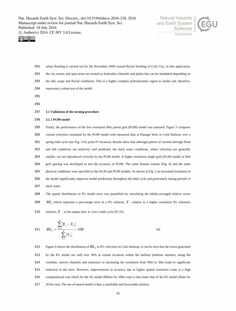
Firstly, the performance of the low resolution 90m parent grid (PG90) model was assessed. Figure 5 compares 299

current velocities simulated by the PG90 model with measured data at Passage West in Cork Harbour over a 300

spring tidal cycle (see Fig. 3 for point P1 location). Results show that although pattern of currents through flood 301

and ebb conditions are relatively well predicted, the slack water conditions, where velocities are generally 302

smaller, are not reproduced correctly by the PG90 model. A higher resolution single grid (SG30) model at 30m 303

grid spacing was developed to test the accuracy of PG90. The same domain extents (Fig. 4) and the same 304

physical conditions were specified to the SG30 and PG90 models. As shown in Fig. 5 an increased resolution of 305

the model significantly improves model predictions throughout the tidal cycle and particularly during periods of 306

slack water. 307

The spatial distribution of PG model error was quantified by calculating the tidally-averaged relative errors 308

TRE which expresses a percentage error in a PG solution, Y , relative to a higher resolution SG reference 309

solution, X , at the output time n over a tidal cycle (N=25) 310

100

1

1 ⋅−

=

∑

∑

=

=N

nn

N

nnn

T

X

XYRE (4) 311

Figure 6 shows the distribution of TRE in PG velocities in Cork Harbour; it can be seen that the errors generated 312

by the PG model are well over 30% at certain locations within the harbour (harbour entrance, along the 313

coastline, narrow channels and estuaries) so increasing the resolution from 90m to 30m leads to significant 314

reduction in the error. However, improvements in accuracy due to higher spatial resolution come at a high 315

computational cost which for the SG model (80min for 50hrs run) is nine times that of the PG model (9min for 316

50 hrs run). The use of nested model is then a justifiable and favourable solution. 317


12

In the course of extensive validation, the timeseries of PG90 and SG30 were also inter-compared. Figure 7 318

shows water elevations and current velocities in Lough Mahon (see Fig. 3 for point C1 location). Water 319

elevations computed by both models are in very good agreement. In contrast, current velocities are significantly 320

overpredicted by the PG90 model. Linear regression of current speeds of PG90 against SG30 solution is shown 321

in Fig. 8. As can be seen from this figure the correlation coefficient between PG90 and SG30 is 0.89 while slope 322

and intercept are m=1.24 and c=0.03, respectively. 323

324

3.1.2 CG30 model 325

The selection of a child grid domain configuration is sensitive to the location of boundaries that may affect the 326

overall stability and performance of the nested model solution. Suitable CG boundaries must be located in areas 327

of low PG inaccuracy and at a sufficient distance from the area of interest as location of the boundary close to 328

the area of interest may result in boundary errors propagating into the area causing the accuracy of the solution 329

to deteriorate. On the other hand, boundaries need to be sufficiently close to the area of interest in order to 330

minimize the domain size (computational cost). 331

The first level child grid, CG30, was located in the north-west part of Cork Harbour with the centrally located 332

Lough Mahon (directly feeding to the River Lee estuary) being the area of interest. The boundaries for the CG30 333

domain were chosen based on the TRE distribution plot for the PG90 current velocities presented in Fig. 6. The 334

upper section of Passage West, connecting Lough Mahon with Lower Harbour, was selected as a suitable 335

southern boundary (SB) due to its relatively low TRE while the closest suitable location for the eastern 336

boundary (EB) was at a much greater distance from Lough Mahon due to generally high PG inaccuracies in the 337

North Channel. 338

The accuracy of the CG30 boundary location was assessed by comparing the net fluxes of mass and momentum 339

across the corresponding interfaces in the PG90, SG30 and CG30 models. Net fluxes were calculated normal to 340

boundaries. Mass and momentum fluxes through the SB and EB boundaries are compared in Fig. 9 and 10, 341

respectively. It can be seen that the predominant forcing-boundary for the CG30 domain is the SB boundary. 342

The tidally-averaged errors in PG90 fluxes relative to the SG30 were approximately 4% for both mass and 343

momentum indicating a high level of PG90 accuracy. At the EB boundary, the PG90 accuracy was slightly 344

lower resulting in error in PG90 mass flux of 5% and momentum flux of 10%. However, this boundary 345

accounted for a smaller portion of the total boundary forcing, and its distant location from the area of interest 346

allowed boundary errors more time to dissipate. The tidally-averaged errors in CG30 fluxes (both mass and 347


13

momentum) relative to PG90 fluxes were less that 2% at both boundaries, demonstrating high levels of 348

conservation from parent grid to child grid. 349

Relative error analysis was also carried out for the entire CG30 model domain with respect to water elevations 350

and velocities, and results of these analyses are summarized in Table 2. The domain-averaged relative error351

DRE ( NRET /= ) in the PG90 water elevations relative to the SG30 were 5.9% while in the CG30 model 352

this error was reduced to 1.1%. The extent of the domains with TRE greater than 1% was 94% for PG90 and 353

28% for CG30. The absolute error defined as: 354

N

XYAE

N

nnn

T

∑=

−= 1 (5) 355

was also calculated. TAE in water level significantly decreased from 8cm in the PG90 to 1.2 cm in the CG30. 356

In relation to current velocities, the DRE was reduced from a large value of 22.4% in PG90 to just 0.5% in 357

CG30; while TRE values exceeding 5% were found in 72% and 4% of the PG90 and CG30 domains, 358

respectively. 359

As shown in Fig. 7, timeseries of water elevations and current speed show very good agreement between SG30 360

and CG30 throughout the tidal cycle. This indicates significant improvement in the accuracy of velocity 361

computation using the high resolution nested CG30 and is verified by the linear regression analysis shown in 362

Fig. 8. The superiority of CG30 over PG90 model when compared to SG30 is clear and confirmed by a 363

correlation coefficient of 0.99 compared to 0.89. The slope and intercept were also improved for CG30 when 364

compared to PG90; with m=1.01 and c=-0.01 the CG30 against SG30 model solutions lie approximately on the 365

45° line. 366

These results demonstrate that the application of the nested high resolution model results in significant 367

improvement in the accuracy of the model solution over the lower resolution PG solution. Similar to the 368

improvement in model accuracy, an equally significant reduction in computational effort was achieved. For 369

example, the application of MSN_Flood model to level 1 domain nesting yields 21 minutes simulation time for 370

the PG90-CG30 model; this is contrasted by 80 minutes simulation time for the SG30 model. Thus the nested 371

model runs 3.8 times quicker than the single grid model. 372

373

374


14

3.1.3 CG06 model 375

In contrast to the CG30 grid being fully embedded within the PG90 grid, in the second level of nesting CG06 is 376

only partially nested within its parent CG30 (Fig. 4). Approximately 38% of wet cells in CG06 overlap CG30. 377

This is a hybrid boundary structure where the east boundary is prescribed using hydrodynamic data from the 378

parent model while the west boundary is prescribed using measured data. The west boundary is a flow 379

boundary, with River Lee inflows extracted from river gauging station 19011. The east boundary is a water 380

elevation boundary where water elevations are supplied along the boundary by the CG30 model. The location of 381

the latter boundary was selected to correspond to the position of the Tivoli tidal gauge station and therefore to 382

contribute to model validation (see Fig. 3 for location of Tivoli gauge). 383

Validation of the CG06 model is conducted for the flood event of November 2009, which due to a combination 384

of heavy river discharges and high tides coinciding with moderate surges resulted in extensive inundation of the 385

area delineated by this nested grid. Figure 11 compares timeseries of water elevation computed at the CG30-386

CG06 nested boundary (east boundary) against tidal gauge records from the same location. Overall, there is a 387

very good agreement between predicted water elevations and measured data. The high degree of model accuracy 388

is manifested by high correlation (0.992) and a low value of RMS difference (0.022m) shown in Table 3 (model 389

CG06_1). Both the RMSE (0.142m) and centred RMSD (0.141m) indicate that the model is able to reproduce 390

variability of water elevation with a good accuracy (order 0.14m). Further, a small difference between these two 391

statistical measures implies that the mean values of observations and simulation are very close. Interestingly, the 392

accuracy of the CG06 model is improved when a 6 minutes phase shift (one record timestep) between 393

observations and simulation is artificially introduced (model CG06_2 in Table 3). This results in RMSE 394

(RMSD) reduction to 0.106m (0.104m) and an increase of correlation to 0.996. It is deemed then that there is a 395

phase lag between model and observations of approximately one observational timestep. Another aspect of the 396

analysis involved temporal occurrence of an error. As the model-observations discrepancies are observed around 397

low water levels (which is not so significant to this study), by not considering negative water elevations (below 398

0 mOD Malin) the RMSE is further reduced to 0.075m (model CG06_3 in Table 3). Such level of agreement 399

between model and observation is considered to be satisfactory. 400

The effect of horizontal resolution on model skill is also examined. This is carried out by comparing the model 401

performance at 6 m and 2m resolutions. For this purpose a single grid 2m reference model (SG02) covering the 402

area delineated by the CG06 model was developed. Figure 12 presents the distribution of water level TRE in 403

the CG06 solution relative to the SG02 reference solution. In general, errors in CG06 outside the Cork City 404


15

centre are very low (<10%) implying that flooding in the rural area of Cork is well resolved using the 6m grid. 405

In contrast, significantly higher errors are obtained in the Cork City (CG02 domain), and in particularly in areas 406

of narrow dense streets where errors exceed 30%. Here, an increase in model resolution leads to a significant 407

reduction in errors. This implies that next level of nesting is required to improve the model accuracy in the city 408

centre. 409

410

3.1.4 CG02 model 411

Finally, the highest resolution 2m model (CG02), fully embedded within CG06, covers the urban area of Cork 412

City; this area is particularly prone to flooding. In the first step of model skill analysis, water elevations 413

simulated by the CG06 and CG02 models at four locations along the river channel are compared in Fig. 13 and 414

statistically summarized in Table 4. Again, the November 2009 flood event was used as a benchmark. Close to 415

the east boundary, at point CG02_4 (see Fig. 14 for point location), both models perform almost identical and 416

this is visually and statistically confirmed in Fig. 13d and in Table 4, respectively. Discrepancies between the 417

CG06 and CG02 models increase with distance from the nested east boundary and are manifested by overall 418

higher water elevations computed by the coarser CG06 model. Location CG02_2 (Fig. 13b) shows the biggest 419

discrepancy evidenced by the statistical measures RMSE=0.195m, RMSD=0.109m, RMSdiff=-0.181m. Despite 420

overprediction of water elevations by the CG06 model, the general water level trends in the two models are in 421

good agreement (COR=0.997). Another important advantage of a high resolution model is an improved 422

numerical stability of the model solution. As can be seen from Fig. 13 a-c, some infrequent random oscillations 423

in water levels occurring in CG06 from numerical instability due to insufficient grid resolution are not present in 424

the finer CG02 model. 425

The effect of improved horizontal resolution is analysed spatially by means of TRE distribution plots. As 426

shown in Fig. 12, the 2m resolution is essential to resolve small scale processes of complex urban area. Figure 427

14 compares TRE between CG02 and SG02. In general, TRE is quite low at 10% in the western part of the 428

city along river banks increasing in eastward direction to 20% in narrow streets of city centre. This is a 429

considerable improvement when compared to TRE in CG06 relative to SG02. Moreover, as CG02 achieves a 430

similar level of accuracy to SG02 the computational cost is significantly reduced and constitutes enormous 96% 431

saving. 432


16

From this analysis it can be seen that the CG06-CG02 nesting results in a model performance generally 433

comparable to the single grid SG02 model but at a significantly reduced computational cost when compared to 434

the single grid model. 435

The ultimate conclusion from the model validation is that MSN_Flood facilitates significant improvements in 436

model accuracy without incurring the computational expense of high spatial resolution over the entire model 437

domain. The model setup constitutes a rigorous test of model performance and on that basis it can be further 438

concluded that the model is applicable to situations where nested boundaries are located in complex urban 439

floodplains that periodically wet and dry. 440

441

3.2 Urban flood modelling 442

For most of the time, city streets are dry and rivers draining the hinterland are contained within well-defined 443

river banks or walls. However, when extreme flood events occur rivers may burst their banks and the city 444

streets become water conveyance channels. The simulation of the hydrodynamics associated with rapid urban 445

flood events is complex; many significant issues must be addressed such as flooding and drying, spatial 446

resolution, domain definition, frictional resistance and boundary descriptions. When modelling flood events, the 447

mathematical formulation of the nested boundaries that permit flooding and drying is of particular importance. 448

Also, the horizontal resolution necessary to resolve small scale processes must be considered. In particular, 449

these aspects of the MSN_Flood model will be discussed in this section. 450

451

3.2.1 Extreme flood event 452

On the 19th and 20th of November 2009 high River Lee flows combined with high astronomical tides and 453

moderate surge caused localized overtopping/breaching of the river banks resulting in widespread flooding of 454

Cork City. Evolution of the flood wave propagation simulated by the CG02 model is shown in Fig. 15. 455

Maximum flooding was reached at 9:30 on 20/11/2009 around the time of high tide and approximately 5 hours 456

after peak discharge of River Lee. At this juncture over 62ha of Cork City had been flooded. The most affected 457

zone was the city centre located between the north and south channels of the river; this area is a low-lying island 458

that over centuries was gradually reclaimed from marshland and it's low-lying topography combined with the 459

influence of river, estuary and harbour makes the area particularly vulnerable to flooding. 460

The accuracy of the urban inundation simulation was assessed against field observations of inundation extent 461

and maximum heights of flood waters. The observed and modelled ultimate extents of flooding in the city are 462


17

shown in the Fig. 16; the hindcasted extent of inundation matches very well that observed during the flood 463

event. With regards to flood level heights, observed water level marks were collected and post-processed by 464

OPW at 38 survey points across the flooded area; their distribution is shown in Fig. 17. The survey point data 465

were subsequently used to calibrate the model. Initial calibration tests showed that the model was most sensitive 466

to bottom roughness coefficient. An extensive statistical analysis of bed roughness parameterization was used to 467

provide an accurate model solution for flood inundation; details of that analysis are presented elsewhere. The 468

best fitting results (R=0.97, RMSD=0.26) were obtained for the following roughness values: upper 469

channel=0.90, lower channel=0.90, roads=0.1, city floodplain=0.1 and upstream floodplain=0.30. Figure 18 470

provides visual assessment of the best fit model skill; good agreement between the model and observations is 471

achieved as the model solution falls on the 45° line. Interestingly, better agreement was found for survey 472

locations in floodplains as opposed to points adjacent to the river bank. This could be attributed to the fact that 473

the majority of survey points are located away from the channel edge (many are actually at the floodplain edge). 474

475

3.3 Moving boundary 476

The specification of a nested boundary in a flood-prone area is particularly problematic; nested models 477

developed so far prohibit flooding and drying along open boundaries. This problem has been overcome in 478

MSN_Flood; its unique mathematical formulation of the nested boundary involving ghost cells, internal 479

boundary formulation and adaptive interpolation, ensures stable flooding and drying of boundary cells. In 480

MSN_Flood, any nested boundary can be placed within a flooding and drying zone and therefore may be subject 481

to significant lateral expansion and contraction. Moreover, the internalization of the boundary allows the 482

flooding and drying mechanism to approach the boundary of the nested domain from either upstream or 483

downstream. As the boundary alternatively floods or dries, the number of active boundary cells expands and 484

contracts accordingly. Depending on local topography, not only the length of the boundary may change but also 485

the number of active boundaries changes. Such a boundary is therefore a complex, non-continuous, moving 486

boundary that spatially and temporally changes its characteristics. This is a significant aspect of this research. 487

In the model setup, the urban CG02 model is entirely embedded within the CG06 model; mass and momentum 488

from the 6m model is transferred to the 2 m model via two nested boundaries – the western boundary 489

transferring River Lee waters from the upper to the lower channel of the river (it also geographically divides the 490

floodplains into upper and lower floodplains), and the eastern boundary exchanging waters with the estuary. The 491

western boundary of CG02 is located on the upstream fluvial floodplain which is prone to wetting and drying. A 492


18

cross section through this boundary illustrating the steep gradients of the river channel bathymetry and the 493

topography of the adjacent urban floodplains (which includes buildings) is shown in Fig. 19. The temporal 494

progression of water levels throughout the November 2009 flooding is also plotted. The reference water level at 495

simulation time t=4hr corresponds to a 187 m3/s river flow (19th of November 2009 at 01:30). At this juncture 496

the flow greatly exceeds the average river flow of 40 m3/s as it results from increased discharges from Inniscarra 497

dam. The storage capacity of Inniscarra Reservoir had been reached after a month-long period of record high 498

rainfalls and heavy downpours on the 18th and 19th of November. Over the course of the subsequent 28 hours 499

the discharges further increased to reach a maximum value of 560 m3/s at 2:30 on November 20th. The water 500

level at the boundary increased from 4.57 mOD at 22:30 November 18th to a peak of 5.74 mOD 28 hours later. 501

The extensive inundation of the upper channel floodplains (upstream floodplains) has a major effect on the 502

western boundary of the CG02 model. It can be seen in Fig. 19 that as the flooding progresses to a simulation 503

time of 8hrs a second wetted boundary is created south of the main channel boundary due to bifurcation of 504

flood waters into two channels (called here the main and side channels) approximately 1.2km upstream of the 505

boundary. Importantly, there is a significant difference in water elevation of 0.41m between the two channels of 506

the boundary. This results from the topography of the upstream floodplains and therefore local flow conditions. 507

The reason for the difference in water elevations along the two sections of the boundary can be explained with 508

the help of Fig. 20 showing three cross-sections including one (cross-section 3) located close to the nested 509

western boundary. As simulated by the CG06 model, downstream from cross-section 1, representing the 510

maximum cross-sectional extent of the inundated area, flood waters must flow around an elevated strip of rural 511

land and so splits at this point into two floodplain channels. This is shown in cross-section 2, located at mid 512

length of this 1 km long strip of land; here the water elevation difference between two channels is 0.31m. This 513

elevation difference further increases to 0.41m near the nested boundary (cross-section 3). 514

The temporal rise of water levels at a number of points across the western nested boundary is shown in Fig. 21. 515

Series A represents the main river channel, series B and C correspond to points adjacent to the river channel 516

while series D is located in the side channel. The difference in water elevations between the two boundaries is 517

apparent throughout the entire flooding period, though it is reduced with the progress of flooding. 518

An interesting characteristics of the moving boundary is it change in its length. As flood waters continue 519

overtopping the river banks, the area of inundation increases and is reflected in the elongation of the boundary. 520

The length of the main channel boundary is initially equal to the river width, this nearly doubles during flooding 521


19

as shown for t=12 hrs in Fig. 19. The temporal evolution of flooding through the boundary clearly demonstrates 522

that the nested boundary is a discontinuous moving boundary with a variable head. 523

The numerical stability of such dynamically changing properties of nested boundary is an important aspect of 524

nesting procedures. Overall, a change in length as well as division into separate subsections does not markedly 525

impact computational stability nor model performance. In fact, as shown in Fig. 14, TRE computed over the 526

flooding period remain low within the CG02 domain despite significant changes to nested boundary 527

configurations and flow conditions. 528

As demonstrated in this section MSN_Flood is developed in a general-purpose manner that through stable and 529

accurate moving boundary provides a high degree of choice and flexibility regarding the location of the 530

boundaries to the nested domain. 531

532

3.4 Model resolution 533

Due to the highly irregular topography of urban environments and the highly dynamic flows involved, urban 534

flooding is a complex problem. Most of the flood models developed so far have focused on rural or semi 535

developed floodplains where isolated large structures can be modelled while small objects are ignored or 536

parameterized as bottom friction (Brown et al., 2007). Such modelling does not implicitly account for locking 537

effects of building on flow. As the presence of buildings may substantially increase flood extent when compared 538

with undeveloped floodplains the role of high resolution discretization is paramount. However, as Brown et al., 539

(2007) found, the greatest source of modelling error with respect to grid resolution is associated with the 540

steepest gradients in topography which are susceptible to interpolation error. 541

Modelling of flood flow through urban area is difficult because of its need for stable and accurate solution of the 542

flow equation (Brown et al., 2007). Since accurate modelling requires a resolution commensurate with flow 543

features, dense street network flows through urban floodplains can only be fully resolved with a sufficiently 544

high resolution. However, satisfactory model resolution, and thus accuracy, incurs computational expense; a 545

balance between these two contradicting factors provides an optimal solution. Gallegos et al. (2009) found that a 546

5m resolution mesh that spans a street by approximately three cells achieves such balance. The characteristics of 547

urban residential areas of southern Californian investigated in their study is different than that of an old 548

European development type towns comprising of narrow dense streets as Cork City. It follows that the 5m 549

model resolution is insufficient to resolve flow dynamics in such city centre street networks. 550


20

In order to analyse the overall effect of model resolution on simulation results, CG06 and CG02 model results 551

are compared. Visual comparison of flood inundation can be made from Fig. 22 which shows CG06 and CG02 552

model outputs representing the maximum extent of inundation during the November 2009 flooding. There is a 553

discrepancy in the extent and magnitude of flooding between the two models. Some zones and streets do not get 554

flooded in the CG06 model, which may be caused by the coarse representation of the street network and 555

associated lack of connectivity between certain streets, while in other zones flood water is present in areas 556

which remain dry according to observations and CG02 output. Figure 23 (a) shows the difference in water 557

elevations between CG02 and CG06 interpolated onto the 2m grid. It is clear that both the height and area of 558

flooding are affected. The absolute difference in water level is on average 0.13m and is underestimated by the 559

6m model by up to 0.4m in the upper section of river and overestimated by approximately 0.3m in the lower 560

section. Figure 23 (b) shows a spatial distribution of RMSE between two models. There is a noticeable reduction 561

in model performance at coarser resolution of 0.08m RMSE over the entire domain and the error is generally 562

larger in the dense street network of the urbanized zone. Based on model results it is clear that a substantial 563

portion of the error results from the coarse representation of topography since its gradient is greater that the 564

slope in water surface; however, some small portion of the error could be attributed to errors in LIDAR data 565

(~0.1m RMSE according to Bates et al, 2010) as well as interpolation from 6m down to 2m grid. 566

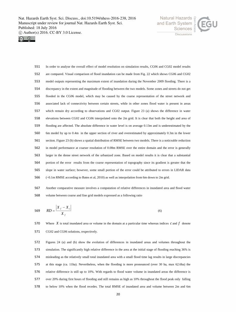
Another comparative measure involves a computation of relative differences in inundated area and flood water 567

volume between coarse and fine grid models expressed as a following ratio 568

f

cf

XXX

RD−

= (6) 569

Where X is total inundated area or volume in the domain at a particular time whereas indices c and f denote 570

CG02 and CG06 solutions, respectively. 571

Figures 24 (a) and (b) show the evolution of differences in inundated areas and volumes throughout the 572

simulation. The significantly high relative difference in the area at the initial stage of flooding reaching 36% is 573

misleading as the relatively small total inundated area with a small flood time lag results in large discrepancies 574

at this stage (ca. 11ha). Nevertheless, when the flooding is more pronounced (over 30 ha, max 62.6ha) the 575

relative difference is still up to 10%. With regards to flood water volume in inundated areas the difference is 576

over 20% during first hours of flooding and still remains as high as 10% throughout the flood peak only falling 577

to below 10% when the flood recedes. The total RMSE of inundated area and volume between 2m and 6m 578


21

models are 3.4ha and 21,367m3. This comparison demonstrates that horizontal resolution is of paramount 579

importance when simulating flows through complex topography. It seems that for Cork City centre comprising 580

of dense network of narrow streets, neither the 5m resolution requirement nor 3 cell street span would resolve 581

complex flood flow at satisfactory level of accuracy. 582

583

3.5 Flood water velocities 584

Another significant advantage of MSN_Flood is its ability to simulate the velocities of flood waters. As oppose 585

to simplified 2D hydraulic models frequently used in urban flooding, the hydrodynamic MSN_Flood includes 586

both the continuity and momentum equations, solving for both water elevations and water velocities. Figure 25 587

shows an example of flood water velocities computed by MSN_Flood in a selected area of Cork city centre 588

blown up for ease of viewing; one can see flood waters in both the river channel and the urban floodplain. This 589

zone is characterized by fast flowing shallow water subject to rapid transitions as it flows down through the 590

steep section of recreational grounds adjacent to the river channel. The city downtown, in contrast, is a ponding 591

area with relatively stagnant waters. 592

Knowledge of velocity fields facilitates better understanding of flood water hydrodynamics and in particular the 593

mechanisms of flood propagation. The routes and speeds of flood waves provide important information for the 594

evaluation of flood risks to people's safety and to property, as well as to the planning and actions of emergency 595

response teams. 596

597

4 Discussion 598

Inundation of coastal areas due to coastal and/or fluvial urban flooding mechanisms is a very complex 599

hydrological phenomena, and developing a modelling system to accurately simulate it is not a trivial task. The 600

research presented in this paper demonstrates that the concept of nesting models is very suitable for complex 601

urban coastal flooding as they facilitate the development of an integrated system capable of resolving 602

hydrodynamics at spatial scales commensurate with flows and physical features of the region of interest. The 603

modelling system adopted here determines physical processes simultaneously at different scales ranging from 604

bay-size circulation (90 m) through mesoscale processes of coastal waters at 30 m resolution down to the ultra-605

high scale environment of 2m. Validation results show that the model performs well at each of these scales. 606

The MSN_Flood model developed for use in this research is well suited for high resolution urban flood 607

simulation for a number of reasons. Firstly, it allows smooth transition of the model solution between coastal 608


22

waters and river floodplains while giving a very high level of conservation of mass and momentum between 609

parent and child grid (Nash and Hartnett, 2010). Through incorporation of ghost cells and formulation of a 610

dynamic internal boundary, MSN_Flood is designed to minimize boundary formulation error and therefore to 611

transfer mass and momentum across the nested boundary without loss of nested solution accuracy. The 612

reduction in boundary errors yields also a significant improvement in model stability at the nested boundary and 613

CG accuracy. This in turn permits stable flooding and drying at the boundary; moreover, these process are 614

allowed to approach the boundary of the nested domain from either upstream or downstream. The so-called 615

moving boundary allows then embedding of a child grid model within the parent model in areas where the 616

nested boundary may wet or dry making the model highly flexible in application. Interestingly, such highly 617

reduced boundary formulation errors is achieved in a nesting mechanism where the nested boundary comprises 618

of only two cells of columns or rows (ghost cells and internal boundary cells). For comparison, in many nested 619

models poor accuracy due to boundary formulation errors is commonly compensated by indirect solutions such 620

as boundary configuration (e.g. location). For example, Kashefipour et al. (2002) in order to reduce possible 621

nesting error dynamically link 2D coastal model with 1D river model by using overlapping grids at the 622

boundary – a common area where boundary values are exchanged between two models. Such model setup is 623

not required in MSN_Flood where accurate exchange of boundary conditions occurs along a boundary. 624

Secondly, the model has virtually no limit to the number of specified nesting levels (and spatial resolution) and 625

is primarily constrained by computational effort rather than numerical stability. The highest resolution of 2 m set 626

for this study was dictated solely by the resolution of available LiDAR data and higher resolutions are easily 627

achievable if suitable terrain data is available. For example, a 0.025 m resolution was used to simulate flows 628

corresponding to those in a physical scale model of a harbour of dimensions 1.0x1.0x0.25 m (Nash and Hartnett 629

2014). In this way, the model allows improved accuracy of solution when compared to a lower resolution parent 630

model where the improved accuracy is similar to that of a similar high resolution single grid model but the 631

computational effort is significantly reduced. 632

Thirdly, the model provides adequate solutions at scales sufficient for processes of interest, such as coarse 633

resolution coastal circulation and fine resolution flood inundation. This is attributed to the robust hydrodynamic 634

module which in essence adopts the well-tested numerical scheme and discretisation methods described by 635

Falconer and Chen (1991). The uniqueness and improvement of MSN_Flood over other nested models is its 636

formulation of the nested boundary in the area where flooding and drying may occur. In order to accommodate 637

flooding and drying of boundary cells the model allows a moving nested boundary so that large sections of the 638


23

boundary can alternatively wet and dry. The stable flooding and drying of boundary cells results from the 639

internalisation of the nested boundary combined with an adaptive interpolation technique tailored specifically 640

for this model. To the author’s knowledge the development of a non-continuous moving nested boundary in a 641

circulation model is novel. Such an innovative solution does not pose restrictions on the location of nested grids 642

with regards wetting and drying (as demonstrated by the application to Cork Harbour) and, therefore, allows 643

flexibility of model setup. 644

Finally, in the context of urban flood modelling, MSN_Flood's ability to simulate horizontal components of 645

water velocity is a significant advantage over simpler hydraulic models commonly used in flood modelling; the 646

complexity of urban topography (buildings, vegetation, walls, roads, embankments, ditches etc) necessitates at 647

least two-dimensional treatment of surface flows (Cook and Merwade, 2009). Spatial and temporal distribution 648

of velocity fields is also required for assessment of flood risk to people and property associated with a certain 649

flood flow magnitude. Thus, this feature will greatly benefit flood hazard management. 650

Although the modelling framework seems to be the main factor controlling accuracy of model predictions, other 651

factors such as model resolution, datasets and model parameterization also play a crucial role. In relation to 652

model topography/bathymetry, these aspects are interconnected and need to be considered jointly. Comparing 653

the 6m and 2 m grid models it can be seen that results are quite sensitive to the spatial resolution of the model. 654

The resolution acts as a filter on the model terrain so the model error increases with decreasing spatial 655

resolution, as the definition of topographic features (walls, hedges etc) are progressively lost from the model 656

bathymetry. There is a dual effect of this. Firstly, as the resolution becomes less granular the topographic 657

complexity of high density small features become sub-grid phenomena which then become parameterised 658

through roughness coefficients. Spatially varying roughness needs to be specified for different terrains, this is 659

determined based on surface classification (such as land type, vegetation or roads) within model sensitivity and 660

calibration. Secondly, the loss of larger objects such as buildings makes the model inherently ill-conditioned and 661

their loss cannot be remedied through modification of roughness coefficient alone. Errors are additionally 662

amplified by a presence of bias in the topographic data resulting from LIDAR related post-processing 663

difficulties such as representation of surface objects discussed in Mason et al. (2003). 664

665

5 Conclusions 666

In this research, high-resolution multi-scale modelling of coastal flooding due to tides, storm surges and rivers 667

inflows is performed. A state-of-the-art modelling system, MSN_Flood, for simulation of coastal flood 668


24

inundation using dynamic downscaling through a cascade of multiple nested grids, was developed to provide a 669

methodology for accurate assessment of flood inundation. A comprehensive assessment of the modelling system 670

was carried out for the coastal city of Cork, which is frequently subject to flooding. A November 2009 extreme 671

flood event driven by both coastal and fluvial mechanisms was selected as a study case. In its application to 672

Cork City, the flood model comprises of four dynamically nested grids that resolve the hydrodynamics of Cork 673

Harbour and Cork City at four different scales: 90m, 30m, 6m and 2m. The urban flood model of 2m horizontal 674

grid resolution is used to simulate flood water inundation of Cork City. 675

The main findings from this research divided into two thematic groups are summarised here: 676

1. Model computational performance: 677

(a) The nesting model framework allows the model operation at practically any desired horizontal 678

resolution, including scales commensurate with resolution of LiDAR data making an optimal use of 679

such datasets. In the current setup, a four-nest cascade telescopes resolution down to the level of 680

LiDAR resolution which is sufficient to capture small scale flow features. 681

(b) The model has no limits as to the number of nesting levels and the numerical stability is maintained 682

down to the finest resolution. 683

(c) Computational effort is dictated by the number of nesting levels, the horizontal resolution of each 684

nested grid and the extents of each nested grid. Nevertheless, at the finest resolution the nested model 685

was found to be almost as accurate as a single grid model of the same resolution but at 96% saving in 686

computational cost. 687

(d) Due to its robust flooding and drying routine, the model maintains numerical stability and accuracy in 688

any part of the model domain affected by these processes. 689

(e) Internalisation of the nested boundary through a use of ghost cells combined with a tailored adaptive 690

interpolation technique permits flooding and drying of the nested boundary creating highly dynamic 691

moving boundaries. Moreover, the flooding and drying mechanism can approach the boundary of the 692

nested domain from either upstream or downstream. Nesting with a moving boundary allows 693

embedding of a child grid model within the parent model in areas where the nested boundary may wet 694

or dry. This unique feature of MSN_Flood provides a high degree of choice regarding the location of 695

the boundaries to the nested domain and therefore flexibility in model application. This capability gives 696

MSN_Flood significant advantages over other models. 697

698


25

2. Model accuracy: 699

(f) The modelling system demonstrates a good capability to accurately determine physical processes at 700

different spatial scales including mesoscale coastal water circulation (90m) and small scale 701

hydrodynamics of complex urban floodplains (2m). 702

(g) The extent of flood inundation into floodplains of Cork City and maximum water levels reached during 703

flooding were accurately simulated by the urban flood 2 m grid model. 704

(h) Fine horizontal resolution is crucial for accurate assessment of inundation. Comparison of 6m and 2m 705

grid model RET in water levels shows a noticeable reduction in model performance at coarser resolution 706

over the entire domain and the error is generally greater in the dense street network of urbanized zone. 707

(i) The urban flood model provides full characteristics of water levels and flow regimes necessary for 708

assessment of flood risk to people's safety associated with particular flood water levels and associated 709

flood water velocities. 710

711

To conclude, near-unlimited model resolution, geographically unconstrained (due to wetting and drying) nested 712

model setup, robust wetting and drying routine, computational efficiency and the capability to simulate both 713

water elevations and velocity fields, make the MSN_Flood a valuable tool for studying coastal flood inundation. 714

This research demonstrates that the adopted methodology can be successfully used in applications to coastal 715

flood modelling including complex urban environments. It can provide, at specific instances of time, accurate 716

spatial distributions of water elevations and flow magnitudes in inundated areas and can, thus, provide critical 717

information to assess possible extents of flood inundation, periods of inundation, maximum water elevations 718

reached and flood wave propagation routes and speeds. Ultimately, it can be directly used for evaluation of 719

flood risks to the area and indirectly, through some functional relationships, for risk assessment of human safety 720

and property damage. The methodology explored in this research, when applied in a forecasting sense, 721

constitutes a high resolution flood warning and planning system that can aid local decision makers targeting 722

high flood risk areas. 723

724

Acknowledgements 725

This publication has emanated from research conducted with the financial support of Science 726

Foundation Ireland (SFI) under Grant Numbers SFI/12/RC/2302 and SFI/14/ADV/RC3021. 727

728


26

References 729

Bates, P.D., Dawson, R.J., Hall, J.W., Horritt, M.S., Nicholls, R.J., Wicks, J., Hassan, M.A.A.M.: Simplified 730

two-dimensional numerical modelling of coastal flooding and example applications. Coastal Engineering 52, 731

795-810, 2005. 732

Bates, P.D., De Roo, A.P.J.: A simple raster-based model for flood inundation simulation. Journal of Hydrology 733

236, 54-77, 2000. 734

Bates, P.D., Horritt, M.S., Fewtrell, T.J.: A simple inertia formulation of the shallow water equations for 735

efficient two-dimensional flood inundation modelling. Journal of Hydrology 387, 33-45, 2010. 736

Brown, J.D., Spencer, T., Moeller, I.: Modeling storm surge flooding of an urban areas with particular reference 737

to modelling uncertainties; A case study of Canvey Island, United Kingdom. Water Resources research 43, 738

W06402, 2007. 739

Chen, X.: Dynamic coupling of a three-dimensional hydrodynamic mode with a latterly averaged, two-740

dimensional hydrodynamic model. Journal of Geophysical Research 112, C07022, 2007. 741

Cook, A., Merwade, V.: Effect of topographic data, geometric configuration and modelling approach on flood 742

inundation mapping. Journal of Hydrology 377, 131-142, 2009. 743

DHI Software, 2001. Mike 21 flow model: hydrodynamic module user guide. DHI water and Environment. 744

Falconer, R.A.: A mathematical model study of the flushing characteristics of a shallow tidal bay. Proc Inst 745

Civil Eng 2 Res and Theory 77, 311-332, 1984. 746

Falconer, R.A., Chen, Y.P.: An improved representation of flooding and drying and wind stress effects in a 2-D 747

tidal numerical model. Proc Inst Civil Eng 2 res and Theory 91, 659-678, 1991. 748

Fewtreel, T.J., Duncan, A., Sampson, C.C., Neal, J.C., Bates, P.D.: Benchmarking urban flood models of 749

varying complexity and scale using high resolution terrestrial LiDAR data. Physics and Chemistry of the Earth 750

36, 281-291, 2011. 751

Formaggia, L., Gerbeau, J.F., Nobile, F., Quarteroni A.: On the coupling of 3D and 1D Navier-Stokes equations 752

for flow problems in compliant vessels. Comput Methods Appl Mech Eng 191, 561-582, 2001. 753

Gallegos, H.A., Schubert, J.E., Sanders, B.F.: Two-dimensional high-resolution modelling of urban dam-break 754

flooding: A case study of Baldwin Hill, California. Advances in Water Resources 32, 1323-1335, 2009. 755

Gomes-Pereira, L.M., Wicherson, R.J.: Suitability of laser data for deriving geographical data: a case study in 756

the context of management of fluvial zones. Photogrammetry and Remote Sensing 54, 105-114, 1999. 757


27

Haidvogel, D.B., H. Arango, W.P. Budgell, B.D. Cornuelle, E. Curchitser, E. Di Lorenzo, K. Fennel, W.R. 758

Geyer, A.J. Hermann, L. Lanerolle, J. Levin, J.C. McWilliams, A.J. Miller, A.M. Moore, T.M. Powell, A.F. 759

Shchepetkin, C.R. Sherwood, R.P. Signell, J.C. Warner, J. Wilkin: Ocean forecasting in terrain-following 760

coordinates: Formulation and skill assessment of the Regional Ocean Modeling System. J. Comp. Phys. 227(7), 761

3595-3624, 2008. 762

Halcrow: Lee catchment flood risk assessment and management study. Hydrology report. Halcrow Group 763

Ireland Ltd. , 2008. 764

Holt, J., Harle, K, Proctor, R., Michel, S., Ashworth, M., Batstone, C., Allem, I., Holems, R., Smyth T., Haines, 765

K., Bretherton, D., Smith G.: Modelling the global coastal ocean. Philos Trans Soc A 367, 939-951, 2009. 766

Horritt, M.S.: Calibration and validation of a 2-dimensional finite element flood flow model using satellite radar 767

imaginary. Water Resources Research 36, 3279-3291, 2000. 768

Horritt, M.S., Bates, P.D., Mattinson, M.J.: Effects of mesh resolution and topographic representation in 2D 769

finite volume models of shallow water fluvial flow. Journal of Hydrology 329, 306-314, 2006. 770

Hunter, N.M., Bates, P.D., Neelz, S., Pender, G., Villanueva, I., Wright, N.G., Liang, D., Falconer, R.A., Lin, 771

B., Waller, S., Crossley, A.J., Mason, D.C.: Benchmarking 2D hydraulic models for urban flooding. Water 772

Management 161, 13-30, 2008. 773

Kashefipour, S.M., Lin, B., Harris, E., Falconer, R.A.: Hydro-environmental modelling for bathing water 774

compliance of an estuarine basin. Water Research 36, 1854-1868, 2002. 775

Korres, G., Lascaratos, A.: A one-way nested eddy resolving model of the Aegean and Levantine Basins: 776

implementation and climatological runs. Ann Geophys 21, 205-220, 2003. 777

Lin, B., Falconer, R.A.: Tidal flow and transport modelling using ULTIMATE QUICKEST scheme. Journal of 778

hydraulic Engineering 123, 303-314, 1997 779

McMillian, H.K., Brasington, J.: Reduced complexity strategies for modelling urban floodplan inundation. 780

Geomorphology 90, 226-243, 2007. 781

Mark, O., Weesakul, S., Apirumanekul, C., Aroonnet S.B., Djordjevic, S.: Potentials and limitations of 1D 782

modelling of urban flooding. Journal of Hydrology 299, 284-299, 2004. 783

Marks, K., Bates, P.D.: Integration of high-resolution topographic data with floodplain flow models. 784

Hydrological processes 14, 2109-2122, 2000. 785


28

Mason, D.C., Cobby, D.M., Horritt, M.S., Bates, P.D.: Floodplain friction parameterization in two-dimensional 786

river flood models using vegetation heights derived from airborne scanning altimetry. |Hydrological Processes 787

17, 1711-1732, 2003. 788

Mason, D.C., Horrit, M.S., Hunter, N.M., Bates, P.D.: Use of fused airborne scanning laser altimetry and digital 789

map data for urban flood modelling. Hydrological Process 21, 1436-1447, 2007. 790

Nash, S.: Development of an adaptive mesh inter-tidal circulation model. PhD Thesis Collage of Engineering 791

and Informatics, National University of Ireland, Galway, 2010. 792

Nash, S., Hartnett, M.: nested circulation modelling of inter-tidal zones: details of nesting approach 793

incorporating moving boundary. Ocean Dynamics 60, 1479-1495, 2010. 794

Nash, S, Hartnett, M.: Development of a nested circulation model: boundary error reduction. Environmental 795

Modelling and Software 53, 65-80, 2014. 796

Nittis, K., Perivoliotis, L., Korrea G., Tziavos, C., Thanos, I.: Operational monitoring and forecasting for marine 797

environmental applications in the Aegean sea. Environ Modell Softw 21, 243-257, 2006. 798

Olbert A.I., Hartnett M.: Storms and surges in Irish coastal waters. Ocean Modelling 34, 50–62, 2010. 799

Pappenberger, F., Beven, K., Horritt, M., Blazkova, S.: Uncertainty in the calibration of effective roughness 800

parameters in HEC-RAS using inundation and downstream level observations. Journal of Hydrology 302, 46-801

69, 2005. 802

Pender, G., Neelz, S.: Benchmarking of 2D hydraulic modelling packages. SC080035/R2 Environmental 803

Agency, Bristol, p. 169, 2010. 804

Ponte, R.M.: Understanding the relation between wind- and pressure-driven sea level variability. Journal of 805

Geophysical Research 99, 8033-8039, 1994. 806

Robins, P.E., Davies, A.G., Jones, R.:Application of coastal model to simulate present and future inundation and 807

aid coastal management. J Coast Conserv 15, 1-14, 2011. 808

Sanders, B.F., Schubert, J.E., Detwiler, R.L.: ParBreZo: A parallel, unstructured grid, Godunov-type, Shallow 809

water code for high-resolution flood inundation modelling at the regional scale. Advances in Water Resources 810

33, 1456-1467, 2010. 811

Simmons A.J., Burridge D.M., Jarraud M., Girard C., Wergen W.: The ECMWF medium-range prediction 812

models development of the numerical formulations and the impact of increased resolution. Meteorol Atmos 813

Phys 40, 28-6, 1989. 814


29

Smith, L.C.: Emerging applications of interferometric synthetic aperture radar (INSAR) in geomorphology and 815

hydrology. Annals Assoc Am Geography 92, 385-398, 2002. 816

Uppala, S.M., Kallberg, P.M., Simmons, A.J., Andrae, U., Bechtold, V., Fiorino, M., Gibson, J., Haseler, J., 817

Hernandez, A., Kelly, G., Li X., Onogi, K., Saarinen, S., Sokka, N., Allan, R., Andersson, E., Arpe, K., 818

Balmaseda, M., Beljaars, A., Berg, L., Bidlot, J., Bormann, N., Caires, S., Dethof, A., Dragosavac, M., Fisher, 819

M., Fuentes, M., Hagemann, S., Holm, E., Hoskins, B., Isaksen, L., Janssen, P., McNally, A., Mahfouf, J., 820

Jenne, R., Morcrette, J., Rayner, N., Saunders, R., Simon, P., Sterl, A., Trenberth, K., Untch, A., Vasiljevic ,D., 821

Viterbo, P., Woollen, J.: The ERA-40 reanalysis. Quart J Roy Meteorol Soc 131, 2961-3012, 2005. 822

Yang, Z., Wang, T., Khangaonkar, T., Breithaupt, S.: Integrated modelling of flood flows and tidal 823

hydrodynamics over coastal floodplains. Environmental Fluid Mechanics 12, 63-80, 2012. 824

Yu, D., Lane, S.N.: Urban fluvial flood modelling using two-dimensional diffusion-wave treatment: 1. Mesh 825

resolution effects. Hydrological Processes 20, 1541-1565, 2006. 826

827

828

829

830

831

832

833

834

835

836

837

838

839

840

841

842

843


30

Tables 844

845

Table 1. Configuration of nested models 846

Model Grid size

m

Timestep

s

Parent model Parent-to-model

grid ratio

Parent grid (PG90) 90 18 -- 1:1

Single grid (SG30) 30 6 PG90 1:1

Child grid 1 (CG30) 30 6 PG90 3:1

Child grid 2 (CG06) 6 0.6 CG30 5:1

Child grid 3 (CG02) 2 0.2 CG06 3:1

Single grid (SG02) 2 0.2 CG06 1:1

847

848

Table 2. Summary of error analyses for PG90 and CG30 models within CG30 model area. 849

Error Analyses

Parameter

SG30

PG90 CG30

Water Elevation:

- RED [%]

- AED [x10-2 m]

- RET > 1% [%]

5.9

8.0

94

1.1

1.2

28

Current Velocity:

- RED [%]

- AED [x10-3 m/s]

- RET > 5% [%]

22.4

2.70

72

0.5

0.13

4

850

851

852


31

Table 3. Error statistics of water elevations simulated by the CG06 model and measured at Tivoli tidal gauge 853

station. Heights are in meters 854

Code COR NSD RMSD

RMSE

RMSdiff

CG06_1 0.992 1.021 0.141 0.142 0.022

CG06_2 0.996 1.023 0.104 0.106 0.024

CG06_3 0.995 1.084 0.075 0.075 0.020

855

856

Table 4. Error statistics of water elevations at four locations simulated by the CG06 and CG02 models. Heights 857

are in meters 858

Code COR NSD RMSD

RMSE

RMSdiff

CG02_1 0.995 1.033 0.080 0.111 -0.081

CG02_2 0.997 1.014 0.109 0.195 -0.181

CG02_3 0.998 1.045 0.056 0.076 -0.064

CG02_4 0.999 0.999 0.006 0.006 0.000

859

860

861

862

863

864

865

866

867

868

869


32

Figures 870

871

872

Figure 1: The nesting procedure for a single level of nesting and one variable only - water surface elevation, ζ . 873

874

875

876

Figure 2: Schematic illustration of the internal boundary configuration for 3:1 nesting ratio. 877

878

∆tp

1st half-timestep 2nd half-timestep

ζ t ζ t+∆tp Interpolation

∆tc

ζ t ζ t+ ½∆tc ζ t+∆tc

t + ∆tp t + 2∆tp t

t

1

2 3 4

5

6 7 8

Parent

Child


33

879 Figure 3: Map of Cork Harbour with selected locations. 880

881

882

Figure 4: Four-level nesting structure of Cork Harbour and City nested model. 883

884

R. Lee

Lough Mahon

Passage West

Passage East

Great Island

Lower Harbour

Tivoli

C1 P1

Cork City


34

885

Figure 5: Comparison of computed and measured velocities at Passage West (point C1 in Figure 3). 886

887

888 Figure 6: RET (%) in PG90 velocities. Black box shows extents of CG30 model and locations of nested 889

boundaries. EB - east boundary, SB – south boundary. 890

891

892

893

EB

SB


35

(a) (b) 894

895

Figure7: Comparison of (a) water elevations and (b) current velocities at point C1 in Lough Mahon. 896

897

898

899

Figure 8: Comparison of modelled velocities for various grid setups at point C1 in Lough Mahon. Time series 900

data are overlain by a linear trend. 901

902

903

904

905


36

(a) (b) 906

907

Figure 9: Comparison of (a) mass and (b) momentum fluxes across EB boundary; PG90 and CG30 timeseries 908

are coincident. 909

910

(a) (b) 911

912

Figure 10: Comparison of (a) mass and (b) momentum fluxes across SB boundary; PG90 and CG30 timeseries 913

are coincident. 914

915


37

916

Figure 11: Water elevations predicted by the CG06 model and measured at Tivoli tidal gauge station. 917

918

919

920

Figure 12: Water level RET (%) in CG06 relative to SG02 . Black box shows extents of CG02 model and 921

locations of nested boundaries. 922

923

924


38

(a) (b) 925

926

(c) (d) 927

928

Figure 13: Timeseries of water elevations predicted by CG06 and CG02 models at four locations (a) CG02_1, 929

(b) CG02_2, (c) CG02_3, (d) CG02_4. 930

931

932


39

933

Figure 14: Water level RET (%) in CG02 relative to SG02 . Red dots denotes points used in water level analysis 934

(see Figure 13). 935

936

937

Figure 15: Temporal evolution of flood wave through upper and lower floodplain of Cork City during 938

November 2009 flood event modelled by CGO6; contours represent 2-hour intervals. 939

940


40

941

Figure 16: Maps of flood inundation observed by (a) OPW and (b) modelled (contours represent 2-hour 942

intervals). Evolution of modelled flood wave is a combined output of CG06 and CG02 models. 943

944

945

Figure 17: Maximum water levels during November 2009 flood event and water level survey points marked as 946

red dots. 947


41

948

949

Figure 18: Comparison of modelled and observed maximum water elevations at 38 stations. 950

951

952

Figure 19: Cross section through west boundary of CG02 model with water elevation marks for selected time 953

points. 954


42

955

Figure 20:Water elevations at three cross-sections during flooding simulated by CG06. 956

957

Section 1 Section 2 Section 3


43

958

959

Figure 21: Timeseries of water elevations across the western nested boundary of CG02. 960

961


44

962

Figure 22: Comparison of flood extent simulated by (a) CG02 and (b) CG06 models. Contours represent water 963

levels (m). 964

965


45

966

Figure 23: (a) Difference in water elevations (m) between CG06 and CG02 models and (b) RMSE contour plot 967

over time. 968

969

970

971

972

973

974

975


46

(a) (b) 976

977

Figure 24: Evolution of the relative difference in (a) total area of inundation and (b) volume of water in 978

inundated area between CG06 and CG02 models. See text for explanation of relative difference. 979

980

981

Figure 25: Map of velocity contours (m/s) with vectors showing magnitude and direction of velocities in the 982

downstream floodplains of Cork City. 983

984

985


Documents

Development of high -resolution multi -scale m odelling … urban... · In this context , the authors present in this paper for the first time the application of the state-of-the