Embed Size (px)
Citation preview
!!!
!!!
!!!
!!!
!!!
!!!
!!!
!!!
!!!
!!!
!!!
!!!
!!!
!!!
!!!
!!!
!!!
!!!
!!!
!!!
!!!
!!!
!!!
!!!
!!!
!!!
!!!
!!!
!!!
!!!
!!!
!!!
!!!
!!!
!!!
!!!
!!!
!!!
!!!
!!!
!!!
!!!
!!!
!!!
!!!
!!!
!!!
!!!
!!!
!!!
!!!
!!!
!!!
!!!
!!!
!!!
!!!
!!!
!!!
!!!
!!!
!!!
!!!
!!!
!!!
!!!
!!!
!!!
!!!
!!!
!!!
!!!
!!!
!!!
!!!
!!!
!!!
!!!
!!!
!!!
!!!
!!!
!!!
!!!
!!!
!!!
!!!
!!! EidgenossischeTechnische Hochschule
Zurich
Ecole polytechnique federale de ZurichPolitecnico federale di Zurigo
Swiss Federal Institute of Technology Zurich
Asymptotic modelling ofconductive thin sheets
K. Schmidt and S. Tordeux∗
Research Report No. 2008-28September 2008
Seminar fur Angewandte MathematikEidgenossische Technische Hochschule
CH-8092 ZurichSwitzerland
∗Institut de Mathematiques de Toulouse, INSA Toulouse, 31077 Toulouse cedex 4,France ([email protected])
ASYMPTOTIC MODELLING OF CONDUCTIVE THIN SHEETS
Kersten Schmidt1 and Sebastien Tordeux2
Abstract. We derive and analyse models which reduce conducting sheets of a small thickness ε in twodimensions to an interface and approximate their shielding behaviour by conditions on this interface.For this we consider a model problem with a conductivity scaled reciprocal to the thickness ε, whichleads a nontrivial limit solution for ε → 0. The functions of the expansion are defined hierarchically,i.e. order by order. Our analysis shows that for smooth sheets the models are well defined for any orderand have optimal convergence meaning that the H
1-modelling error for an expansion with N termsis bounded by O(εN+1) in the exterior of the sheet and by O(εN+1/2) in its interior. We explicitelyspecify the models of order zero, one and two. Numerical experiments for sheets with varying curvaturevalidate the theoretical results.
1991 Mathematics Subject Classification. 65N30, 35C20, 35J25, 41A60, 35B40, 78M30, 78M35.
Introduction
Many electric devices contain very thin conducting parts either for electromagnetic shielding [13, 16], or ascasings, tank walls [9, 23] or supply lines [5]. The large aspect ratio of these sheets of about few millimetres orcentimetres to metres or hundreds of micrometres to centimetres and the high conductivity causes variationsin thickness direction in much smaller scales than in the longitudinal directions. Their discretisation by thefinite element method (FEM) is challenging when the thickness ε of the thin sheets is considerably smaller thanthe size of neighbouring parts for three reasons. First, domains with such thin sheets are difficult to mesh bymost mesh generators. Secondly, a discretisation on meshes with cell sizes of different magnitudes can lead toill-conditioned matrices, and thirdly, meshes of good quality may also contain cells around the sheet with sizescomparable to the sheet thickness which leads to a high number of additional degrees of freedom. By reducingthe thin sheet to an interface and by approximating its effect by conditions on this interface a highly accuratemodelling with standard discretisation schemes like the FEM is possible.
The so called impedance boundary conditions (IBCs), first proposed by Shchukin [27] and Leontovich [19],are traditionally used for replacing solid conductors, where the domain is artificially confined, by an approximateboundary condition [1–3, 8, 11, 15, 26]. This technique is proved to be accurate for smooth sheets and can bereadily implemented.
However, in the context of thin conducting sheets this technique of Shchukin and Leontovich has beenseldomly applied. Interface conditions for thin sheets are often based on a tensor product ansatz of a set ofsimple functions in thickness direction and functions defined on the interface. The simplest approaches assume
Keywords and phrases: Asymptotic Expansions, Model Reduction, Thin Sheets.
1 Seminar for Applied Mathematics, ETH Zurich, 8092 Zurich, Switzerland2 Institut de Mathematiques de Toulouse, Universite de Toulouse, France
2
no variation in thickness direction, which leads to a surface quantity [5, 22]. Using two functions in thicknessdirection Krahenbuhl and Muller [18] derived a relation between the mean value of the tangential component ofthe electric or magnetic field on the interfaces of the sheet and the jump of the magnetic or electric field betweenthe interfaces. This approach for time-harmonic Maxwell’s equations is adopted by various authors [13, 17, 20]and is known as impedance boundary condition for thin layers. The functions in thickness direction dependingon the frequency ω and the conductivity σ take the skin effect into account. In similar IBCs for simulationsin time domain underlying functions are changed dynamically [6, 21]. Unfortunately, these interface conditionsare of low order, and even with the use of a larger number of functions in thickness direction [14] this type ofconditions do not achieve higher orders [25].
In this paper we derive a high order approximation technique to deal with thin sheets based on argumentssimilar to those that was used to derive IBCs. We attain these approximations in the context of a 2D scalarmodel problem with a smooth thin dissipative sheet.
The model problem defined in Section 1 includes the two major effects, the shielding and the skin effect.We investigate an asymptotics of constant shielding for ε → 0 by scaling the conductivity c like 1/ε. Forthis asymptotics we derive the problems defining together the expansion functions of the solution of arbitraryorder inside and outside the sheet in Section 2. Then, in Section 3 we will rearrange the problems leadingto hierarchical coupled problems defining the expansion functions for each order with the knowledge of thefunctions of previous orders only. We will decouple these problems, introduce their variational formulation andshow existence and uniqueness of the internal and external expansion functions in Section 4. Then, in Section 5we analyse the modelling error and give the models for the first three orders explicitely in Section 6. Finally, wedescribe in Section 7 the numerical discretisation of the asymptotic expansion models and the original model bymeans of high-order finite elements and show results for the modelling error in various indicators in dependenceof the sheet thickness. These numerical simulations demonstrate the sharpness of the bounds for the modellingerror.
1. Problem definition
Let Ω be a domain in R2 and Ωεint be the sub-domain occupied by a sheet of thickness ε > 0 with conductivity
c. The remaining sub-domain Ωεext := Ω\Ωε
int is non-conducting and we denote the conductivity function c(x),where c(x) = c for x ∈ Ωε
int and c(x) = 0 otherwise. We call the sub-domain of the thin conducting sheet theinterior and the non-conducting sub-domain the exterior.
Let uε be the solution of the problem
−∆uε(x) + c(x)uε(x)= f(x) in Ω,uε(x)= g(x) on ∂Ω,
(1)
with the source term f(x) vanishing in Ωεint and the Dirichlet data g(x). This model problem borrows the
eddy-current model in 2D and includes the skin and shielding effects. We use a bounded domain Ω andDirichlet boundary conditions for sake of simplicity. However, the boundary condition is of no importance inthe derivation of the thin sheet models and can be replaced easily, also by suitable radiation conditions for anunbounded domain.
We make the following assumptions on the sheet. The mid-line Γm is given as C∞ continuous and C∞ in-vertible map xm(t) from a 1D torus (note that Γm is hence closed), identified with a reference interval Γ ⊂ R.Furthermore, we assume Γm to have a positive distance to the boundary of Ω, and, for simplicity, |x′
m(t)| = 1,i.e. t is an arc length parameter. The left normed normal vector and the curvature of the sheet are denoted byn(t) and κ(t), and the normal derivative by ∂n = ∇ · n. Hence, we can define a parametrisation of the sheet
x(t, s) = xm(t) + sn(t)
3
(a)
ε
n
s
t
0Ωεext
Ωεext
Ωεint
∂Ω Ω (b)
n
Ω0ext
Ω0ext
Γm
∂Ω Ω (c)
Ω
S
t Γ
0− 12
12
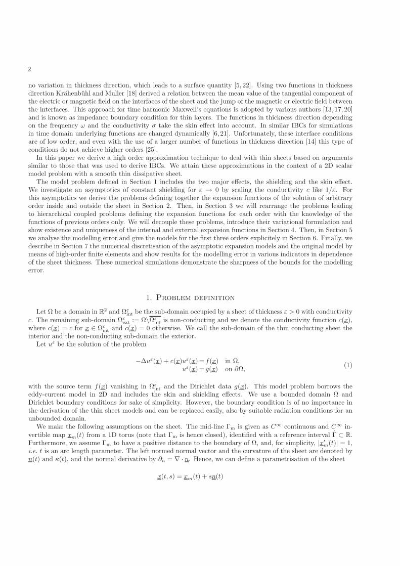
Figure 1. (a) Family of geometries for the family of problems for uε(x). (b) Limit geometryfor ε → 0. (c) Normalised interior sub-domain.
over the parameter domain Ωε := Γ×[− ε
2 , ε2
], where s ∈
[− ε
2 , ε2
](see Figure 1(a)). Due to the regularity of its
midline Γm we can assert for the sheet that
C−1κ ≤ 1 + sκ(t) ≤ Cκ ∀ (t, s) in Ωε, (2)
for ε small enough with a positive constant Cκ. Finally, we denote the interfaces of the sheet for s = ± ε2 by Γε
+
and Γε− and its union by Γε.
For an asymptotic analysis we embed the problem (1) for a sheet of a particular thickness into a family ofproblems with varying thicknesses and a conductivity depending on the respective thickness. There are severalpossible scalings of the conductivity with decreasing thickness ε, e. g. one can consider c = c0
εα for differentparameters α. The choice c = c0/ε is a borderline case between a perfect shielding (α > 1) and no shielding(α < 1) and corresponds asymptotically to a constant shielding [25]. Therefore, this choice is of practicalinterest.
Hence, we look for the solution uε ∈ H1(Ω) satisfying
−∆uεext = f in Ωε
ext,
−∆uεint +
c0
εuε
int =0 in Ωεint, ) c0 ≥ 0,
uεext = g on ∂Ω,
uεext(t,± ε
2 )=uεint(t,± ε
2 ) on Γ,∂nuε
ext(t,± ε2 )= ∂nuε
int(t,± ε2 ) on Γ,
(3)
where we denote by uεext the solution restricted to Ωε
ext and by uεint its restriction to Ωε
int. We assume for apositive constant ε0, that f ∈ C∞(Ωε0
ext), and g ∈ C∞(∂Ω) and ∂Ω to be C∞.
2. Derivation of the coupled problems
In this section, we derive two asymptotic expansions of the exact solution, one in each of the exterior andinterior sub-domains. These two expansions are defined by a coupled problem.
4
2.1. The exterior and interior asymptotic expansions of the solution
The exterior asymptotic expansion corresponds to the asymptotic expansion of uε restricted to Ωεext. It
consists in a formal power series
uεext(x) =
∞∑
i=0
εiuiext(x) + o (ε∞)
ε→0in Ωε
ext, (4)
in which the terms of the asymptotic expansion are independent of ε and defined on Ω0ext = Ω \ Γm (see
Figure 1(c)), the limit of Ωεext for ε → 0.
The interior asymptotic expansion is an asymptotic expansion of uε restricted to Ωεint. In order to introduce
the normalised domain Ω := Γ × [− 12 , 1
2 ] (see Figure 1(c)), we consider the stretched variable
S = ε−1s. (5)
The normalised representation of a function v defined in Ωεint is denoted by its capital letter V : v(x) = v(t, s) =
V (t, S). The interior asymptotic expansion is postulated to be a formal power series in ε
Uεint(t, S) =
∞∑
i=0
εiU iint(t, S) + o (ε∞)
ε→0in Ω, (6)
whose terms Uεint are independent of ε and defined on Ω.
Currently, we do not give a mathematical sense to this expansion, even if the formal computation makessense. The expansion of the exact solution by a power series in ε emerges as a proper choice, because all theexpansions involve only polynomials in ε. This ansatz of a power series in ε will be ultimately validated byTheorem 5.1.
In the remainder of this section we derive a coupled problem defining the functions uiext and U i
int.
The coupled problem
Find the families of functions (uiext)i∈N0
and (U iint)i∈N0
such that for all i ∈ N0
−∆uiext = fδi
0 in Ω0ext, (7a)
uiext = gδi
0 on ∂Ω, (7b)
∂2SU i
int(t, S) = c0Ui−1int (t, S) −
i∑
#=1
∆#Ui−#int (t, S) in Ω. (7c)
U iint(t,± 1
2 ) − uiext(t,±0) =
i∑
#=1
(±
1
2
)# 1
( !∂#
sui−#ext (t,±0) on Γm, (7d)
∂SU iint(t,± 1
2 ) =i∑
#=1
(±
1
2
)#−1 1
(( − 1)!∂#
sui−#ext (t,±0), on Γm. (7e)
where we use the Kronecker symbol, δij = 1 if i = j and δi
j = 0 if i += j, and the differential operators ∆# for( ∈ N which are given by
∆#(t, S) = ∆0# (t)S
#−2 + ∆1# (t)S
#−1∂S ,
∆0# (t) = (−κ(t))#−2(( − 1)
(∂2
t +( − 2
2
κ′(t)
κ(t)∂t
)and ∆1
# (t) = −(−κ(t)) #.(8)
5
Equations (7a) and (7b) are readily to derive by inserting (4) in (3) and identifying terms of the same order in ε.More steps, however, are needed to obtain the leading equation for U i
int. It relies on the asymptotic expansion
∆ = ε−2∂2S +
L−1∑
#=1
ε#−2∆# + εL−2RLε for all L ≥ 1 (9)
of the Laplacian expressed in local coordinates [8, 25]
∆ = ∂2s +
κ(t)
1 + sκ(t)∂s +
1
1 + sκ(t)∂t
(1
1 + sκ(t)∂t
)
= ε−2∂2S +
ε−1κ(t)
1 + εSκ(t)∂S +
1
1 + εSκ(t)∂t
(1
1 + εSκ(t)∂t
)with (t, s) = (t, Sε), (10)
where for its remainder it holds for any L ∈ N
‖RLε U‖L2(bΩ) ≤ CL ‖U‖H2(bΩ)
Inserting (4) and (9) in (3) leads to equation (7c). The coupling conditions (7d) and (7e) need a specifictreatment that will be detailed in Section 2.2.
Remark. The first terms of the expansion of the Laplacian are required in the sequel
∆0 = ∂2S , ∆1 = κ(t)∂S , ∆2 = ∂2
t − κ2(t)S∂S . (11)
2.2. The Dirichlet and Neumann coupling conditions
In this section we derive the transmission conditions (7d) and (7e). These relations result from the exactDirichlet and Neumann transmission conditions on Γm written in local coordinates
uεext(t,± ε
2 ) = Uεint(t,± 1
2 ), (12)
∂suεext(t,±
ε
2) =
1
ε∂SUε
int(t,± 12 ). (13)
Since these conditions are written at s = ±ε/2, Taylor expansions of uiext expressed on Γm will be used to
obtain conditions on a single interface. They require regularity of uiext that will be a posteriori validated in
Theorem 4.4, by assuming smoothness of Γm.Remark. The interfaces between the thin sheet and the exterior domain consist of two parts (s = ±ε/2).
Even if one decides to shift the position of the mid-line Γm (s = 0), at least one of the interfaces is not fixedwith respect to ε. This leads to rather more complicated coupling conditions than for thin coatings [2, 3, 8],where the interface consists of one part only and can be fixed independently of ε.
The Dirichlet transmission condition (7d).
The Taylor expansion of uiext reads
uiext(t,±
ε
2) =
∞∑
j=0
(±
ε
2
)j 1
j!∂j
suiext(t,±0) + o (ε∞)
ε→0. (14)

6
Inserting the expansion (4), (6) and (14) into (12), we obtain
0 = uεext(t,± ε
2 ) − Uεint(t,± 1
2 )
=∞∑
i=0
εi
∞∑
j=0
(±
ε
2
)j 1
j!∂j
suiext(t,±0) − U i
int(t,± 12 )
+ o (ε∞)ε→0
=∞∑
i=0
εi
i∑
j=0
(±
1
2
)j 1
j!∂j
sui−jext (t,±0) − U i
int(t,± 12 )
+ o (ε∞)ε→0
. (15)
Identifying terms of same orders leads to the Dirichlet transmission condition (7d).Remark.The exterior expansion functions ui
ext may be discontinuous across Γm.
The Neumann transmission condition (7e).
The Taylor expansion of ∂suiext reads
∂suiext(t,±
ε
2) =
∞∑
j=0
(±
ε
2
)j 1
j!∂j+1
s uiext(t,±0) + o (ε∞)
ε→0. (16)
Inserting the expansions (4), (6) and (16) into (15), we get
0 = ε∂suεext(t,±
ε
2) − ∂SUε
int(t,± 12 )
=∞∑
i=0
εi
ε∞∑
j=0
(±
ε
2
)j 1
j!∂j+1
s uiext(t,±0) − ∂SU i
int(t,± 12 )
+ o (ε∞)ε→0
=∞∑
i=0
εi
( i−1∑
j=0
(±
1
2
)j 1
j!∂j+1
s ui−j−1ext (t,±0) − ∂SU i
int(t,± 12 )
). (17)
Identifying terms of the same order results in the Neumann transmission condition (7e).
3. The hierarchical coupled problem
In the last section, we derived a coupled problem (7) that defines the families of exterior and interiorterms (ui
ext)i∈N and (U iint)i∈N. However, these equations do not define the family hierarchically. Indeed, given
(U iint, u
iext)i<k, (7) written for i = k, and not for all i ∈ N, does not uniquely define (Uk
int, ukext). This is due to
the fact that there is no condition for the normal derivative ∂sukext(x) on the mid-line Γm.1
Deriving a necessary condition for the existence U i+1int leads to a formulation of (7) which permits the com-
putation of (U iint, u
iext)i≤k step by step.
1Remember, that for second order differential equations two transmission conditions are needed. We have with (7d) a Dirichlettransmission condition and (7e) defines the normal derivative from the interior. Thus, a condition for the normal derivative fromthe exterior of the sheet is missing.
7
Symbols for the mean and the jump
For the sake of brevity let us introduce the following symbols for the jumps and the mean values of theexpansion functions
[V ](t) := V (t, 12 ) − V (t,− 1
2 ), V (t) :=1
2
(V (t, 1
2 ) + V (t,− 12 )),
[v](t) := v(t, 0+) − v(t, 0−), v (t) :=1
2
(v(t, 0+) + v(t, 0−)
),
and a symbol for either the jump or the mean value of the external expansion function of both sides of themid-line Γm
[v]n (t) :=
[v](t) n even
2 v(t) n odd.
The latter symbol is convenient for terms resulting from the Taylor expansions (14) and (16), in which the signchanges from term to term and, hence, the difference is the jump and the mean value, in turns.
Additional condition for the normal derivative ∂suiext(x)
The missing condition for the normal derivative ∂suiext(x) is the compatibility condition for (7c) and (7d)
which is necessary for the existence of the internal functions U i+1int . Inserting (7c) and (7e) into the following
equality for U iint
0 = ∂SU iint(t, +
12 ) − ∂SU i
int(t,− 12 ) −
∫ 12
− 12
∂2SU i
int(t, S) dS,
we obtain
0 =i∑
#=1
(1
2
)#−1 1
(( − 1)!
[∂#
sui−#ext
]#−1(t) −
∫ 12
− 12
(c0U
i−1int (t, S) −
i∑
#=1
∆#Ui−#int (t, S)
)dS. (18)
Furthermore, inserting the equality ∆1 = κ(t)∂S (see (11)) we can rewrite (18) for i = i + 1 as
∫ 12
− 12
(c0 − κ(t)∂S
)U i
int(t, S) dS −[∂su
iext
](t) =
i∑
#=1
(∫ 12
− 12
∆#+1Ui−#int (t, S) dS +
1
2# ( ![∂#+1
s ui−#ext ]#(t)
), (19)
which is a condition for the normal derivative involving only terms of order i. Adding this condition to (7)yields a problem which defines the expansion functions hierarchically.
8
The hierarchical coupled problem
For i ∈ N0, find uiext and U i
int such that
−∆uiext = fδi
0 in Ω0ext, (20a)
uiext = gδi
0 on ∂Ω, (20b)
∂2SU i
int(t, S) = c0Ui−1int (t, S) −
i∑
#=1
∆#Ui−#int (t, S) in Ω, (20c)
U iint(t,± 1
2 ) − uiext(t,±0) =
i∑
#=1
(±
1
2
)# 1
( !∂#
sui−#ext (t,±0) on Γm, (20d)
∂SU iint(t,± 1
2 ) =i∑
#=1
(±
1
2
)#−1 1
(( − 1)!∂#
sui−#ext (t,±0) on Γm, (20e)
∫ 12
− 12
(c0 − κ(t)∂S
)U i
int(t, S) dS −[∂su
iext
](t) =
i∑
#=1
(∫ 12
− 12
∆#+1Ui−#int (t, S) dS +
(1
2
)# 1
( ![∂#+1
s ui−#ext ]#(t)
)on Γm. (20f)
Remark. It can be easily proven that U iint(t, S) is a polynomial of degree 2i in S for i ∈ N0. Thus, we define
U0int(t) := U0
int(t, S).In the next section, we prove the existence and uniqueness of the solution of problem (20).
4. Well-posedness of the hierarchical coupled problem
4.1. An algorithm to solve the hierarchical coupled problem
In this section we propose an algorithm to define successively the three functions
U iint(t, S) := U i
int(t, S) − U iint(t), ui
ext(x) and U iint(t). (21)
as the solutions of the following three problems which can be solved iteratively:(i) Find U i
int(t, S) : Ω −→ C such that
∂2SU i
int(t, S) = c0Ui−1int (t, S) −
i∑
#=1
∆#Ui−#int (t, S) in Ω,
∂SU iint(t,±
1
2) =
i∑
#=1
(±
1
2
)#−1 1
(( − 1)!∂#
sui−#ext (t,±0) on Γm,
U iint(t) = 0 on Γm.
(22a)
9
(ii) Find uiint(t, S) : Ω0
ext −→ C such that
−∆uiext = fδi
0 in Ω0ext,
uiext = gδi
0 on ∂Ω,
[ui
ext
](t) =
[U i
int
](t) −
i∑
#=1
(1
2
)# 1
( !
[∂#
sui−#ext
]#(t) on Γm,
[∂su
iext
](t) − c0
ui
ext
(t) =
∫ 12
− 12
c0Uiint(t, S) dS − κ(t)
[U i
int
](t)+
i∑
#=1
(c0
(1
2
)# 1
( ![∂#
sui−lext ]
#+1(t) on Γm,
−(
1
2
)# 1
( ![∂#+1
s ui−#ext ]#(t)
−∫ 1
2
− 12
∆#+1Ui−#int (t, S) dS
).
(22b)
(iii) Find U iint : Γm −→ C such that
U iint(t) =
ui
ext
(t) +
i∑
#=1
(1
2
)# 1
( ![∂#
sui−#ext ]#+1(t) on Γm. (22c)
Lemma 4.1. The problem (22) is equivalent to the problem (20).
Proof. We first demonstrate that every solution of (20) is also a solution of (22). The equations (22a) area direct consequence of (20c) and (20e) taking into account that U i
int(t) is a constant in S. The equation(22c) follows by applying the mean value operator to (20d). The third equation in (22b) follows by applyingthe jump operator to (20d). And, the fourth equation of (22b) is obtained, after calculation, by insertingU i
int(t, S) = U iint(t, S) + U i
int(t) and (22c) into (20f).Applying the converse arguments, we can show that every solution of (22) is also solution of (20). !
4.2. Variational framework
The interior solution uiext is defined by the system (22b). This section is devoted to the existence, uniqueness
and regularity of the solution of such problems.Given f ∈ L2(Ω), g ∈ H
12 (∂Ω), γ ∈ H
12 (Γm), δ ∈ H− 1
2 (Γm), we are looking for solution u ∈ H1(Ω0ext) of the
problem
−∆u = f, in Ω0ext,
u = g, on ∂Ω,
[u] = γ, on Γm,
[∂nu] − c0u = δ, on Γm.
(23)
10
A classical route to deal with this non-homogeneous problem consists in introducing the harmonic offset functionu ∈ H1(Ω0
ext) satisfying
∆u = 0, in Ω0ext,
u(·,±0) = ± 12γ(·), on Γm,
u = g, on ∂Ω.(24)
Consequently, u fulfils the jump condition [u](t) = γ and has a vanishing mean u(t) = 0. Moreover, since∆u = 0 in Ω0
ext and u ∈ H1(Ω0ext), the jump of the normal trace [∂nu] belongs to H− 1
2 (Γm).Multiplying the first equation of (23) by a test function v, integrating over Ω and using the Green formula,
we get the following weak formulation for u = u − u :
Find u ∈ H10 (Ω) such that a(u, v) = l(v) ∀v ∈ H1
0 (Ω), (25)
with the bilinear form a(·, ·) and the linear form l(·) defined by
a(u, v) :=
∫
Ω∇u ·∇v dx +
∫
Γm
c0 uv dt, (26)
l(v) :=
∫
Ωfv +
∫
Γm
([∂nu] − δ) v dt. (27)
Using Poincare-Friedrichs inequality [7], it is rather easy to prove the following lemma.
Lemma 4.2. The system (23), with data f ∈ L2(Ω), g ∈ H1/2(∂Ω), γ ∈ H1/2(Γm) and δ ∈ H−1/2(Γm) admits aunique solution given that ) c0 ≥ 0.
Even if we seek the expansion functions u ∈ H1(Ω0ext) they possess a higher regularity given that the mid-
line of the sheet Γm and the source term f are smooth enough. This confirms the validity of the Taylorexpansions (14) and (16).
Proposition 4.3. For k0 ∈ N, f ∈ Hk0−2(Ω0ext), g ∈ Hk0−1/2(∂Ω), γ ∈ Hk0−1/2(Γm), δ ∈ Hk0−3/2(Γm) and
Γm ∪ ∂Ω Ck0-continuous, let u(x) ∈ H1(Ω0ext) be the solution of (23).
For any positive integer k ≤ k0, there exists a constant Ck > 0 such that
‖u‖Hk(Ω0ext)
≤ Ck
(‖f‖Hk−2(Ω0
ext)+ ‖g‖Hk−
1/2(∂Ω) + ‖γ‖Hk−1/2(Γm) + ‖δ‖Hk−
3/2(Γm)
).
Proof. Applying the techniques of Proposition 2.8 in [25] we get the statement of proposition. !
Remark. If the boundary of the domain is not smooth enough, the regularity statement of Proposition 4.3 hasto be restricted to a sub-domain of Ω0
ext excluding a neighbourhood of the boundary. A sub-domain of Ω0ext
exluding the support of the source term f has to be taken, if this term is not smooth.
4.3. Existence and uniqueness of (uiext) and (U i
int)
Theorem 4.4. The sequences (uiext) and (U i
int) exist and are uniquely defined by (22). For any k ∈ N0 and
i ∈ N0 it holds uiext ∈ Hk(Ω0
ext), U iint ∈ Hk(Ω), and U i
int ∈ Hk(Ω) and consequentely U iint ∈ Hk(Ω) as well.
Proof. The proof is by induction in i.For i = 0, the Sturm-Liouville problem (22a) with homogeneous data uniquely defines U0
int(t) = 0 (see [28]for a presentation of Sturm-Liouville problems). The source term and the mid-line of the sheet are C∞ byassumption. Thus, by Proposition 4.3 there exists for any k ∈ N a constant C0,k such that ‖u0
ext(t)‖Hk(Ω0ext)
≤
11
C0,k. Since H1(Ω0ext) ⊂ L2(Ω0
ext) the same holds for k = 0. By (22a) we can assert that U0int,0(t) = U0
int(t) =
U0int(t) =
u0
ext
(t) ∈ Hk−1/2(Γm) for any k ∈ N. Hence, the statement of the theorem is proven for i = 0.
Assume that the assertion holds for all integer j < i. We divide the rest of the proof in three steps. In (i) weprove the existence, uniqueness and regularity of U i
int (i), in (ii) those of uiext and in (iii) the regularity of U i
int.
(i) The function U iint is defined by the Sturm-Liouville problem (22a). This function exists and is unique
if and only if the source terms satisfy the compatibility2 condition (18). This condition is fulfilled sinceit is equivalent to (20f) written for i = i − 1 which holds as (ui−1
ext , U i−1int ) is the solution of (22) and by
Lemma 4.1 also of (20). The regularity of U iint follows from the regularity of (uj
ext)j<i and (U jint)j<i.
(ii) The function uiext is defined by (22b). Since (uj
ext)j<i, (U jint)j<i and U i
int are regular, the existence,uniqueness and regularity of ui
ext result from Lemma 4.2 and Proposition 4.3.(iii) The function U i
int is defined by (22c). The smoothness of U iint follows from the regularity of (uj
ext)j≤i.
!
Remark. Although we assume a smooth boundary ∂Ω and a smooth source term f , this assumption is notneeded for the existence and uniqueness of the expansion functions (Theorem 4.4) since the former terms of theexpansion (uj
ext)j<i appear only on the mid-line Γm and regularity is required for the traces to this mid-line only.
5. Estimates of the modelling error
To obtain an approximation uε,N of order N ∈ N0 of the exact solution uε we truncate the expansions ofuε
ext and Uεint to the first N + 1 terms
uε,Next (x) :=
N∑
i=0
εiuiext(x), and Uε,N
int (t, S) :=N∑
i=0
εiU iint(t, S), (29)
and use the notation uε,Nint (t, s) := Uε,N
int (t, s/ε). Now, we formulate the main result about the modelling errorin the following Theorem.
Theorem 5.1 (The modelling error in the H1-norm). For any N ∈ N0, there exists a constant CN independentof ε such that
‖uεext − uε,N
ext ‖H1(Ωεext)
+√
ε ‖uεint − uε,N
int ‖H1(Ωεint
) ≤ CNεN+1. (30)
Proof. In order to prove Theorem 5.1 we need to estimate the remainder rε,N+1
rε,N+1ext = uε
ext − uε,Next and rε,N+1
int = uεint − uε,N
int . (31)
In Section 5.1, we identify residuals by inserting rε,N+1 in the model problem (3). Then, these residuals arebounded in Section 5.2. Finally, we conclude using a stability argument in Section 5.3. !
2This compatibility condition corresponds to a necessary condition for the existence of eU iint
:
∂SeU iint(t, +
1
2) − ∂S
eU iint(t,−
1
2) =
Z 12
−
12
∂2S
eU iint(t, S) dS. (28)
12
5.1. The problem for the remainder
Contrary to uε, the approximation uε,N given in (29) does not exactly fulfil our model problem (3). Indeed,the exact solution uε has continuous Dirichlet and Neumann data on Γε, whereas the Dirichlet and Neumanntraces of uε,N have jumps. Moreover, the partial differential equation in the sheet is also not satisfied exactly.More precisely, the remainder rε,N+1 solves the following system of equations
−∆rε,N+1ext = 0 in Ωε
ext,
−∆rε,N+1int +
c0
εrε,N+1int = δε,N+1
int in Ωεint
rε,N+1ext (t,±
ε
2) − rε,N+1
int (t,±ε
2) = δε,N+1
D,± on Γε,
∂srε,N+1ext (t,±
ε
2) − ∂sr
ε,N+1int (t,±
ε
2) = δε,N+1
N,± on Γε,
rε,N+1ext = 0 on ∂Ω,
(32)
with the internal residual
δε,N+1int (x) :=
(−∆ +
c0
ε
)(uε
int(x) − uε,Nint (x)
)(3)= −
(−∆ +
c0
ε
)uε,N
int (x)(29)= −
N∑
i=0
εi(−∆ +
c0
ε
)ui
int(x), (33a)
the residual of the Dirichlet jump
δε,N+1D,± (t) :=
(uε
ext(t,±ε
2) − uε
int(t,±ε
2))
︸ ︷︷ ︸0 by (3)
−(uε,N
ext (t,±ε
2) − uε,N
int (t,±ε
2))
(29)=
N∑
i=0
εi
(U i
int(t,±1
2) − ui
ext(t,±ε
2)
)
(33b)
and the residual of the Neumann jump
δε,N+1N,± (t) :=
(∂nuε
ext(t,±ε
2) − ∂nuε
int(t,±ε
2))
︸ ︷︷ ︸0 by (3)
−(∂nuε,N
ext (t,±ε
2) − ∂nuε,N
int (t,±ε
2))
(29)=
N∑
i=0
εi
(1
ε∂SU i
int(t,±1
2) − ∂nui
ext(t,±ε
2)
). (33c)
5.2. Consistency estimates
In this section, we estimate the residuals δε,N+1int , δε,N+1
D,± and δε,N+1N,± defined in (33).
5.2.1. The internal residual
Proposition 5.2 (Consistency error in the sheet). There exists CN > 0, independent of ε, such that
‖δε,N+1int ‖L2(Ωε
int) ≤ CN εN−1/2.
Proof. We write the interior residual given by (33a) in local coordinates, Dε,N+1int (t, S) := δε,N+1
int (t, s), withs = Sε. Inserting the expansion of the Laplace operator (9) we have
Dε,N+1int (t, S) = −
N∑
i=0
εi
(
−ε−2
(
∂2S +
N−i∑
#=1
(ε#∆#
)+ εN−i+1RN−i+1
ε
)
U iint(t, S) +
c0
εU i
int(t, S)
)
. (34)
13
With the convention U−1int ≡ 0, we collect the terms of same powers of ε
Dε,N+1int (t, S) = εN−1
(N∑
i=0
RN−i+1ε U i
int(t, S) − c0UNint(t, S)
)
+N∑
i=0
εi−2
(
∂2SU i
int(t, S) − c0Ui−1int (t, S) +
i∑
#=1
∆#ui−#int (t, S)
)
︸ ︷︷ ︸0 by (22a)
. (35)
Since U iint(t, S) is independent of ε for all i by Theorem 4.4, we obtain using (9)
∥∥∥Dε,N+1int
∥∥∥L2(bΩ)
≤ εN−1
(N∑
i=0
C‖U iint‖H2(bΩ) + c0‖UN
int‖L2(bΩ)
)
≤ CNεN−1. (36)
Considering the curved geometry, see (2), we can write the integral in the original coordinates
‖δε,N+1int ‖2
L2(Ωεint
) ≤ Cκ
∫
Γ
∫ ε2
− ε2
(δε,N+1int (t, s))2 ds dt = Cκε
∥∥∥Dε,N+1int
∥∥∥2
L2(bΩ)≤ CN ε2N−1.
The proof is complete. !
5.2.2. A preliminary result on the Taylor expansion remainder
In Sections 5.2.3 and 5.2.3, the estimates of the Dirichlet and the Neumann jump residuals will require thefollowing proposition. We give the proof of this classical result for the sake of completeness.
Proposition 5.3 (Estimate of the remainder of the Taylor expansion). Let L ∈ N.
∃CL > 0 ∀ε > 0 ∀u ∈ HL([−ε
2;ε
2] \ 0)
∣∣rLε,±(u)
∣∣ ≤ CL εL−1/2 |u|HL([0,± ε2]) (37)
with rLε,+(u) and rL
ε,+(u) the two reals defined by
rLε,±(u) := u(±
ε
2) −
L−1∑
#=0
(±
ε
2
)#u(#)(±0). (38)
Proof. We use the well-known expression of the remainder term of Taylor polynomials
|rLε,±(u)| =
1
(L − 1)!
∣∣∣∣
∫ ± ε2
0
(±
ε
2− s
)L−1∂L
s u(s) ds
∣∣∣∣.
Bounding∣∣± ε
2 − s∣∣L−1
by its maximal value(
ε2
)L−1and applying the Cauchy-Schwarz inequality, we obtain
∣∣∣∣
∫ ± ε2
0
(±
ε
2− s
)L−1∂L
s u(s) ds
∣∣∣∣ ≤(ε
2
)L− 12 ‖∂L
s u‖L2([0,± ε2]) =
(ε
2
)L− 12 |u|HL([0,± ε
2]).
The composition of the estimates completes the proof. !
14
5.2.3. The Dirichlet jump residual
The functions δε,N+1D,± (t) for the Dirichlet jumps are defined on Γε
+ or Γε−, respectively. However, we can
regard them as functions on the mid-line Γm. In the following proposition we bound the L2-norm of the error ofthe Dirichlet jumps evaluated on the mid-line. In Proposition 5.5, we will then define and estimate an extensionfunction of the Dirichlet jump into the sheet.
Proposition 5.4 (Estimate of the Dirichlet jump residual). There exists a constant CN > 0, independentof ε, such that for j = 0, 1
‖∂jt δ
ε,N+1D,± ‖L2(Γm) ≤ CNεN+1/2. (39)
Proof. The Dirichlet jump residual is given by (33b). Replacing uiext(t,± ε
2 ) by its Taylor expansion, see Propo-sition 5.3, we get
δε,N+1D,± (t) =
N∑
i=0
εi
(U i
int(t,±1
2) −
i∑
j=0
(±
1
2
)j 1
j!∂j
sui−jext (t,±0)
)−
N∑
i=0
εirN−i+1ε,± (ui
ext)(t). (40)
Due to (20d), this simplifies to
δε,N+1D,± (t) = −
N∑
i=0
εirN−i+1ε,± (ui
ext)(t). (41)
Applying (37), we get the estimate with CN a generic constant depending on N
|δε,N+1D,± (t)| ≤
N∑
i=0
εi(CN−i εN−i+1/2 ‖∂N−i+1
s uiext‖L2([0,± ε
2])
)≤ CN εN+1/2
N∑
i=0
‖∂N−i+1s ui
ext‖L([0,± ε2]). (42)
Thus, we can bound the L2(Γm)-norm of δε,N+1D,± by a triangular inequality
‖δε,N+1D,± (t)‖L2(Γm) ≤ CN εN+ 1
2
N∑
i=0
‖∂N−i+1s ui
ext‖L2(Γm×[0,± ε2]).
Considering the curvature, C−1κ ≤ 1 + sκ(t) by (2), and since Γm × (0,± ε
2 ] ⊂ Ω0ext we can write
‖∂N−i+1s ui
ext‖2L2(Γm×[0,± ε
2]) ≤ Cκ
∫
Γm
∫ ± ε2
0(∂N−i+1
s uiext(s, t))
2(1 + sκ(t)) ds dt ≤ Cκ|uiext|2HN−i+1(Ω0
ext).
Thus, we obtain ‖∂N−i+1s ui
ext‖L2(Γm×[0,± ε2]) ≤ ‖ui
ext‖HN+1(Ω0ext)
. It follows that
‖δε,N+1D,± (t)‖L2(Γm) ≤ CNεN+ 1
2
N∑
i=0
|uiext|HN−i+1(Ω0
ext)≤ CNεN+ 1
2 ‖uiext‖HN+1(Ω0
ext).
By inserting the regularity bound for the expansion functions uiext (see Theorem 4.4) we obtain
‖δε,N+1D,± (t)‖L2(Γm) ≤ CN,0 εN+1/2,
which is our claim for j = 0. With similar arguments we find
‖∂tδε,N+1D,± (t)‖L2(Γm) ≤ CN εN+ 1
2 ‖∂tuiext‖HN+1(Ω0
ext)≤ CN εN+ 1
2 ‖uiext‖2
HN+2(Ω0ext)
≤ CN εN+ 12 .
This completes the proof. !
15
Proposition 5.5 (An extension function of the Dirichlet jump residual). There exists an extension δε,N+1D (t, s)
of δε,N+1D,± (t) defined in (33b) into Ωε
int with
∂sδε,N+1D
(t,±
ε
2
)= 0, and ∃CN > 0 ∀ε > 0 : ‖δε,N+1
D ‖H1(Ωεint
) ≤ CNεN . (43)
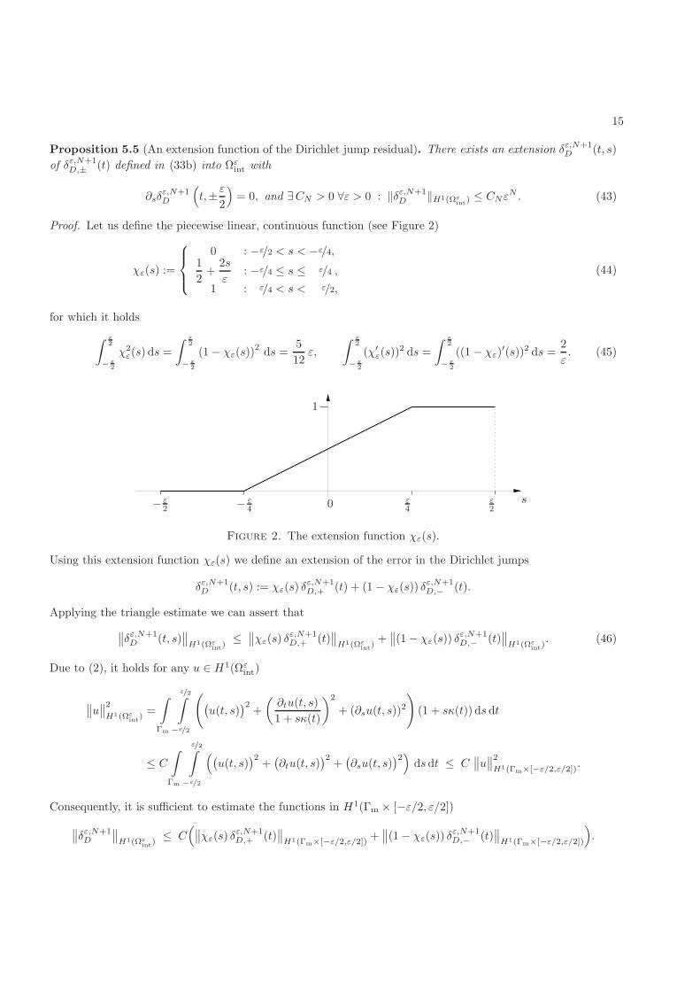
Proof. Let us define the piecewise linear, continuous function (see Figure 2)
χε(s) :=
0 : −ε/2 < s < −ε/4,1
2+
2s
ε: −ε/4 ≤ s ≤ ε/4 ,
1 : ε/4 < s < ε/2,
(44)
for which it holds
∫ ε2
− ε2
χ2ε(s) ds =
∫ ε2
− ε2
(1 − χε(s))2 ds =
5
12ε,
∫ ε2
− ε2
(χ′ε(s))
2 ds =
∫ ε2
− ε2
((1 − χε)′(s))2 ds =
2
ε. (45)
− ε2 − ε
4ε4
ε2
s
1
0
Figure 2. The extension function χε(s).
Using this extension function χε(s) we define an extension of the error in the Dirichlet jumps
δε,N+1D (t, s) := χε(s) δε,N+1
D,+ (t) + (1 − χε(s)) δε,N+1D,− (t).
Applying the triangle estimate we can assert that
∥∥δε,N+1D (t, s)
∥∥H1(Ωε
int)≤
∥∥χε(s) δε,N+1D,+ (t)
∥∥H1(Ωε
int)+∥∥(1 − χε(s)) δε,N+1
D,− (t)∥∥
H1(Ωεint
). (46)
Due to (2), it holds for any u ∈ H1(Ωεint)
∥∥u∥∥2
H1(Ωεint
)=
∫
Γm
ε/2∫
−ε/2
((u(t, s)
)2+
(∂tu(t, s)
1 + sκ(t)
)2
+ (∂su(t, s))2)
(1 + sκ(t)) ds dt
≤ C
∫
Γm
ε/2∫
−ε/2
((u(t, s)
)2+(∂tu(t, s)
)2+(∂su(t, s)
)2)ds dt ≤ C
∥∥u∥∥2
H1(Γm×[−ε/2,ε/2]).
Consequently, it is sufficient to estimate the functions in H1(Γm × [−ε/2, ε/2])
∥∥δε,N+1D
∥∥H1(Ωε
int)≤ C
(∥∥χε(s) δε,N+1D,+ (t)
∥∥H1(Γm×[−ε/2,ε/2])
+∥∥(1 − χε(s)) δε,N+1
D,− (t)∥∥
H1(Γm×[−ε/2,ε/2])
).
16
Due to the tensorial nature of the two terms on the right hand side, we can roughly bound
∥∥δε,N+1D
∥∥H1(Ωε
int)≤ C
(∥∥χε
∥∥H1(Γm)
∥∥δε,N+1D,+
∥∥H1([−ε/2,ε/2])
+∥∥(1 − χε)
∥∥H1(Γm)
∥∥δε,N+1D,−
∥∥H1([−ε/2,ε/2])
).
Inserting the estimates (39) and (45) we finally obtain (43). !
5.2.4. The Neumann jump residual
Proposition 5.6 (Estimate of the Neumann jump residual). There exists a constant CN > 0, independentof ε, such that
‖δε,N+1N,± ‖L2(Γε) ≤ CN εN−1/2.
Proof. The error in the Neumann jump is given by
δε,N+1N,± (x)
(33c)=
N∑
i=0
εi
(1
ε∂SU i
int(t,±1
2) − ∂su
iext(t,±
ε
2)
)
(38)=
N∑
i=0
εi−1
(∂SU i
int(t,±1
2) −
i−1∑
j=0
(±
1
2
)j 1
j!∂j+1
s ui−j−1ext (t,±0)
)
︸ ︷︷ ︸0 by (7e)
−N∑
i=0
εirN−iε,± (∂su
iext)(t)
= −N∑
i=0
εirN−iε,± (∂su
iext)(t),
where we inserted the Taylor polynomial of ∂suiext(t,± ε
2 ) with their remainder terms in the second step. Note,
that rLε,±(∂sui
ext)(t) depends on t ∈ Γ since ∂suiext is a function of t. The terms in the first sum cancel due
to the approximation of the Neumann continuity in (7e). Now, we use (37) to estimate the remainders of thetruncated Taylor expansion:
⇒ |δε,N+1N,± (t)|
(37)≤
N∑
i=0
εi(CN−i εN−i+1/2 ‖∂N−i+2
s uiext‖L2([0,± ε
2])
)
≤ CN εN+1/2
N∑
i=0
‖∂N−i+2s ui
ext‖L2([0,± ε2]).
The proof of the bound in the L2-norms is then similar to the one of Proposition 5.5. !
5.3. Proof of Theorem 5.1
Let rext := rε,N+1ext , rint := rε,N+1
int − δε,N+1D , with δε,N+1
D the extension function of δε,N+1D,± of Proposition 5.5.
Then, the function r is continuous over the interfaces Γε of the sheet and inherits the vanishing trace on theboundary from rε,N+1. It lies consequently in H1
0 (Ω).Multiplying (32) with a test function v ∈ H1
0 (Ω) and integrating by parts in Ωεext and in Ωε
int we get thevariational formulation: Seek r ∈ H1
0 (Ω), such that
∫
Ωεext
∇rext ·∇vext dx +
∫
Ωεint
(∇rint ·∇vint +
c0
εrintvint
)dx =
∫
Γε+
−δε,N+1N,+ v dt +
∫
Γε−
δε,N+1N,− v dt
+
∫
Ωεint
(∇δε,N+1
D ·∇vint +c0
εδε,N+1D vint
)dx +
∫
Ωεint
δε,N+1int v dx. (47)
17
For ) c0 ≥ 0, the left hand side defines a H10 (Ω)-elliptic continuous bilinear form. By the estimates of the
Propositions 5.2, 5.5 and 5.6 the right hand side defines a H1(Ω)-continuous linear form. The Lax-Milgramlemma [24] ensures stability. Inserting the results of the Propositions 5.2, 5.5 and 5.6 yields
‖rε,N+1‖H1(Ω) ≤ ‖r‖H1(Ω) + ‖δε,ND ‖H1(Ωε
int)
≤ C
((2 +
√c0
ε
)‖δε,N+1
D ‖H1(Ωεint
)︸ ︷︷ ︸
O(εN )
+∑
σ=+,−
‖δε,N+1N,σ ‖L2(Γε
σ)︸ ︷︷ ︸
O(εN− 12 )
+ ‖δε,N+1int ‖L2(Ωε
int)
︸ ︷︷ ︸O(εN− 1
2 )
)≤ C εN− 1
2 , (48)
with C > 0 a constant independent of ε. Moreover, by definition (31)
rε,N+1 = εN+1uN+1 + εN+2uN+2 + rε,N+3. (49)
Using the fact that for every integer i, ‖ui‖H1(Ωεext)
= O(1) and ‖ui‖H1(Ωεint
) = O(ε−1/2), inserting (48) into(49) and applying the triangle inequality we conclude that
∥∥∥rε,N+1ext
∥∥∥H1(Ωε
ext)≤ εN+1
∥∥uN+1ext
∥∥H1(Ωε
ext)+ εN+2
∥∥uN+2ext
∥∥H1(Ωε
ext)+∥∥∥rε,N+3
ext
∥∥∥H1(Ωε
ext)
≤ C1εN+1 + C2ε
N+2 + C3εN+3/2 ≤ CεN+1,
∥∥∥rε,N+1int
∥∥∥H1(Ωε
int)≤ εN+1
∥∥uN+1int
∥∥H1(Ωε
int)+ εN+2
∥∥uN+1int
∥∥H1(Ωε
int)+∥∥∥rε,N+3
int
∥∥∥H1(Ωε
int)
≤ C1εN+1/2 + C2ε
N+3/2 + C3εN+3/2 ≤ CεN+1/2.
6. The three first orders
In Section 4, the external function uiext and the internal function U i
int were defined by a coupled problem, see(22). We could use a finite element method for the approximation on two meshes – a first one for Ω0
ext and asecond one for Ω. Since this formulation is not common, we propose an equivalent definition of the internal andexternal functions by uncoupled problems, whose solutions will be much easier to approximate numerically.
More precisely, we elaborate a procedure that allows to compute the exterior functions of order 0, 1, and 2,with no need of the interior functions. This factorisation leads to three problems defining u0
ext, u1ext and u2
ext
involving only exterior fields of lower order, see (56), (62) and (64). The details for the second order will notbe given.
6.1. Preliminary results: replacing higher normal derivatives on the mid-line
The asymptotic expansion models (22) involve derivatives of high order with respect to the normal direction.Because it is from a practical point of view easier to handle tangential derivatives than normal derivatives ofthe same order we intend to replace these higher normal derivatives. Due to the absence of a source term f inΩε
int for all ε smaller than ε0, i.e.
−∆uiext(t, s) = 0, s ∈
[− ε
2 , ε2
], (50)
it is possible to replace the normal derivatives by derivatives in t.Taking the two limits of the expression (10) of the Laplace operator for s → ±0 we obtain
∆ = ∂2n + κ(t)∂n + ∂2
t
and inserting the above expression into (50) yields
∂2nui
ext(t,±0) = −κ(t) ∂nuiext(t,±0) − ∂2
t uiext(t,±0). (51)
18
Applying the normal derivative ∂s to (10) we get the expression
0 = ∂s∆ = ∂3s −
κ2(t)
(1 + sκ(t))2∂s +
κ(t)
1 + sκ(t)∂2
s −κ(t)
(1 + sκ(t))2∂t
(κ(t)
1 + sκ(t)∂t
)
+κ(t)
1 + sκ(t)∂t
(−
κ(t)
(1 + sκ(t))2∂t +
κ(t)
1 + sκ(t)∂s∂t
).
Taking the two limits for s → ±0 we have
∂3nui
ext(t,±0) = −κ(t)∂2nui
ext(t,±0) +(κ2(t) − ∂2
t
)∂nui
ext(t,±0) +(2κ(t)∂2
t + κ′(t)∂t
)ui
ext(t,±0)
(51)=
(2κ2(t) − ∂2
t
)∂nui
ext(t,±0) +(3κ(t)∂2
t + κ′(t)∂t
)ui
ext(t,±0). (52)
Such expressions hold also for the jump and for the mean value of higher order derivatives
[∂2
nuiext
](t)
∂2
nuiext
(t)
= −κ(t)
[∂nui
ext
](t)
∂nui
ext
(t)
− ∂2t
[ui
ext
](t)
ui
ext
(t),
(53)
[∂3
nuiext
](t)
∂3
nuiext
(t)
=(2κ2(t) − ∂2
t
) [
∂nuiext
](t)
∂nui
ext
(t)
+ (3κ(t)∂2t − κ′(t)∂t)
[ui
ext
](t)
ui
ext
(t).
(54)
6.2. Order 0
First, we express the internal function U0int as expression of u0
ext. Then, inserting this expression into (22b)leads to an uncoupled problem for u0
ext.
6.2.1. Internal function
The internal function is given as the sum of the mean value U0int(t) and of the function U0
int(t, S), whichare defined in (22a) and (22c), respectively. By evaluating these equations we find
∂2SU0
int(t, S) = 0
∂SU0int(t,±
1
2) = 0
U0int(t) = 0
⇒ U0
int(t, S) = 0 and U0int(t) = u0
ext(t).
Consequently, the internal function is given by
U0int(t, S) = U0
int(t) = u0ext(t). (55)
6.2.2. External function
Inserting U0int = 0 into (22b) yields the completely uncoupled problem for the external function u0
ext
−∆u0ext(x) = f(x) in Ω0
ext,
u0ext(x) = g(x) on ∂Ω,
[u0
ext
](t) = 0 on Γm,
[∂su
0ext
](t) − c0
u0
ext
(t) = 0 on Γm.
(56)
19
Note that u0ext is uniquely defined by Lemma 4.2. As u0
ext has no jump over Γm we denote u0ext(t) := u0
ext(t,±0) =u0
ext
(t). Thus, we can write the last equation of (56) as
[∂su
0ext
](t) − c0 u0
ext(t) = 0 on Γm. (57)
6.3. Order 1
In the same way as for order 0 we express U1int in terms of u0
ext and u1ext and derive the uncoupled problem
defining u1ext. Then, we replace a second normal derivative by a second tangential and a simple normal derivative.
The resulting model for u1ext depends only on the external function of order 0.
6.3.1. Internal function
The internal function U1int(t, S) is given as the sum of the mean value U1
int(t) and the function U1int(t, S),
which are defined in (22a) and (22c), respectively. For i = 1, the problem (22a) takes the form
∂2SU1
int(t, S) = c0U0int(t) − κ(t) ∂SU0
int(t)︸ ︷︷ ︸0
= c0u0ext(t)
∂SU1int(t,± 1
2 ) = ∂su0ext(t,±0)
U1int(t) = 0.
(58)
Consequently, we can assert that
U1int(t, S) =
c0
2u0
ext(t)(S2 − 1
4
)+∂su
0ext
(t)S. (59)
From (22c) the mean value of the internal function is given by
U1int(t) = u1
ext(t) + 14 [∂su
0ext](t)
(56)= u1
ext(t) +c0
4u0
ext(t), (60)
and we can re-compose the internal function to
U1int(t, S) =
c0
2u0
ext(t)(S2 + 1
4
)+∂su
0ext
(t)S + u1
ext(t). (61)
6.3.2. External function
Inserting (59) into (22b) we obtain a vanishing Dirichlet jump
[u1
ext
](t) =
[U1
int
](t) −
∂su
0ext
(t) =
∂su
0ext
(t) −
∂su
0ext
(t) = 0,
and for the Neumann jump
[∂su
1ext
](t) − c0
u1
ext
(t) =
∫ 12
− 12
c0U1int(t, S) dS
︸ ︷︷ ︸−
c20
12u0ext(t) by (59)
−κ(t)[U1
int
](t)
︸ ︷︷ ︸∂su0
ext(t) by (59)
+c0
4[∂su
0ext](t)︸ ︷︷ ︸
c0u0ext(t) by (57)
− ∂2su0
ext(t) −∫ 1
2
− 12
∂2t U0
int(t, S)︸ ︷︷ ︸
u0ext(t) by (55)
−κ2(t)S ∂SU0int(t, S)
︸ ︷︷ ︸0 by (55)
dS.
20
ba
R
ε
Ωεext
Ωεint
(a)
Γm
(b)
Ωεint
(c)
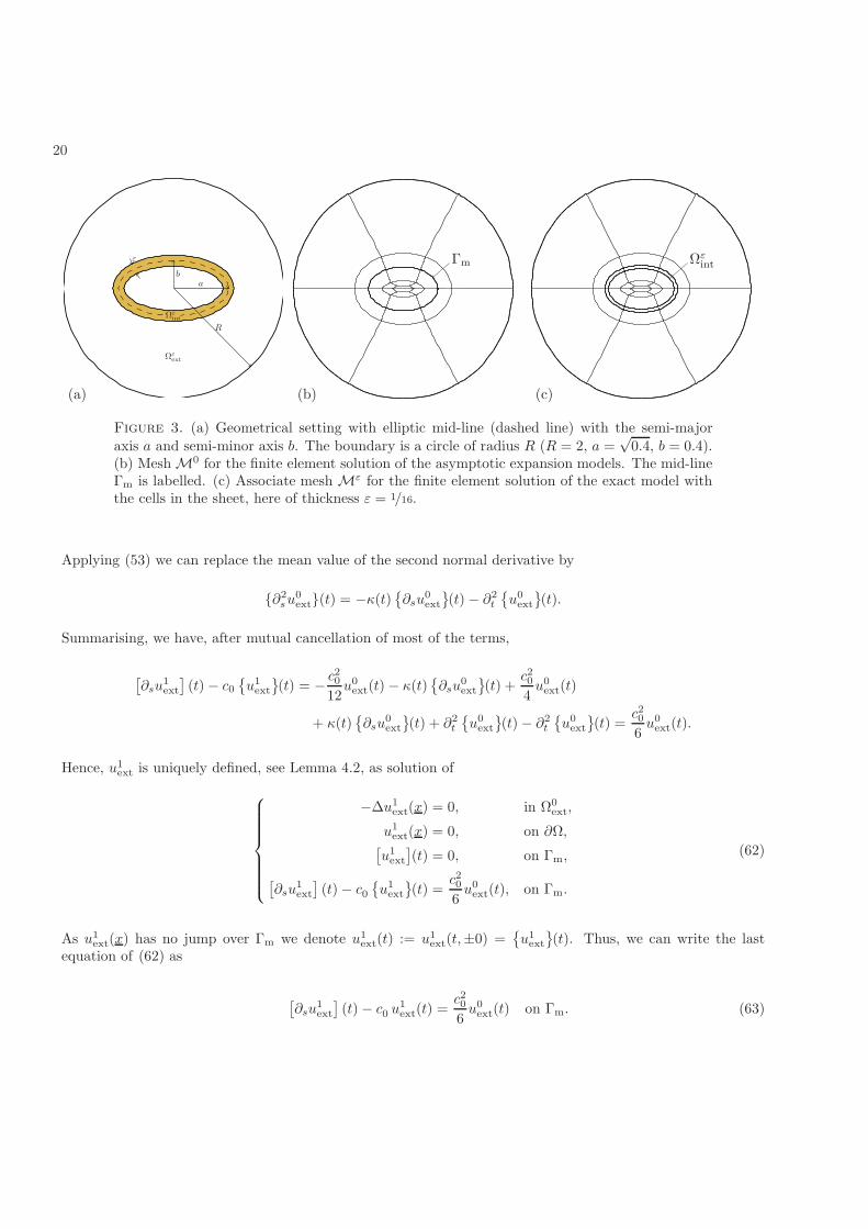
Figure 3. (a) Geometrical setting with elliptic mid-line (dashed line) with the semi-majoraxis a and semi-minor axis b. The boundary is a circle of radius R (R = 2, a =
√0.4, b = 0.4).
(b) Mesh M0 for the finite element solution of the asymptotic expansion models. The mid-lineΓm is labelled. (c) Associate mesh Mε for the finite element solution of the exact model withthe cells in the sheet, here of thickness ε = 1/16.
Applying (53) we can replace the mean value of the second normal derivative by
∂2su0
ext(t) = −κ(t)∂su
0ext
(t) − ∂2
t
u0
ext
(t).
Summarising, we have, after mutual cancellation of most of the terms,
[∂su
1ext
](t) − c0
u1
ext
(t) = −
c20
12u0
ext(t) − κ(t)∂su
0ext
(t) +
c20
4u0
ext(t)
+ κ(t)∂su
0ext
(t) + ∂2
t
u0
ext
(t) − ∂2
t
u0
ext
(t) =
c20
6u0
ext(t).
Hence, u1ext is uniquely defined, see Lemma 4.2, as solution of
−∆u1ext(x) = 0, in Ω0
ext,
u1ext(x) = 0, on ∂Ω,
[u1
ext
](t) = 0, on Γm,
[∂su
1ext
](t) − c0
u1
ext
(t) =
c20
6u0
ext(t), on Γm.
(62)
As u1ext(x) has no jump over Γm we denote u1
ext(t) := u1ext(t,±0) =
u1
ext
(t). Thus, we can write the last
equation of (62) as
[∂su
1ext
](t) − c0 u1
ext(t) =c20
6u0
ext(t) on Γm. (63)
21
6.4. Order 2
6.4.1. External function
In the same way, one can obtain that the second order term u2ext is uniquely defined by (see Lemma 4.2)
∆u2ext(x) = 0 in Ω0
ext,[u2
ext
](t) = −
c0
24κ(t)u0
ext(t, 0) −c0
12
∂nu0
ext
(t) on Γm,
[∂nu2
ext
](t) − c0
u2
ext
(t) =
c20
6u1
ext(t) +c0
24κ(t)
∂nu0
ext
(t)
+ c0
(7
240c20 −
∂2t
12
)u0
ext(t, 0) on Γm,
u2ext(x) = 0 on ∂Ω,
(64)
whose Dirichlet and Neumann traces are both discontinuous over the mid-line of the sheet in general. Thetransmission conditions depend on the solutions of order 0 and 1 and include even a second tangential derivativeof u0
ext. Once again no boundary data or source term is involved.
6.4.2. Internal function
The internal expansion function of order 2 is the fourth order polynomial
U2int(t, S) =
c20
24u0
ext(t)
(S2 +
3
4
)2
+c0
6
∂su
0ext
(t)
(S3 −
3
4S
)−
c0
6κ(t)u0
ext(t)
(S3 +
3
4S
)(65)
+c0
2u1
ext(t)
(S2 +
1
4
)−
1
2
(κ(t)
∂su
0ext
(t) + ∂2
t u0ext(t)
)S2 +
∂su
1ext
(t)S +
u2
ext
(t),
which involves the curvature of the sheet and a second tangential derivative of the external function of order 0.
x
-2
-1
0
1
2
y
-2
-1
0
1
2
0.6
0.7
0.8
0.9
1
uε
(a) ε = 1/8
x
-2
-1
0
1
2
y
-2
-1
0
1
2
0.6
0.7
0.8
0.9
1
uε
(b) ε = 1/16
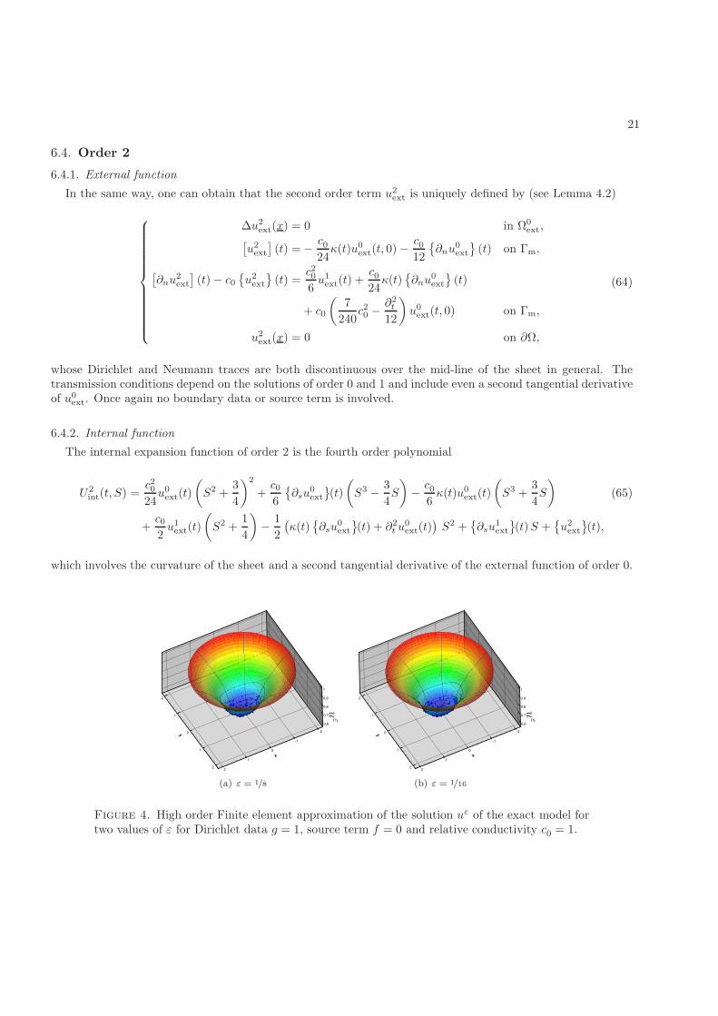
Figure 4. High order Finite element approximation of the solution uε of the exact model fortwo values of ε for Dirichlet data g = 1, source term f = 0 and relative conductivity c0 = 1.
22
x
-2
-1
0
1
2
y
-2
-1
0
1
2
0.6
0.7
0.8
0.9
1
u0ex
t
(a) Order 0
x
-2
-1
0
1
2
y
-2
-1
0
1
2
-0.04
-0.03
-0.02
-0.01
0
u1ex
t
(b) Order 1
x
-2
-1
0
1
2
y
-2
-1
0
1
2
-0.05
0
0.05 u2ex
t
(c) Order 2
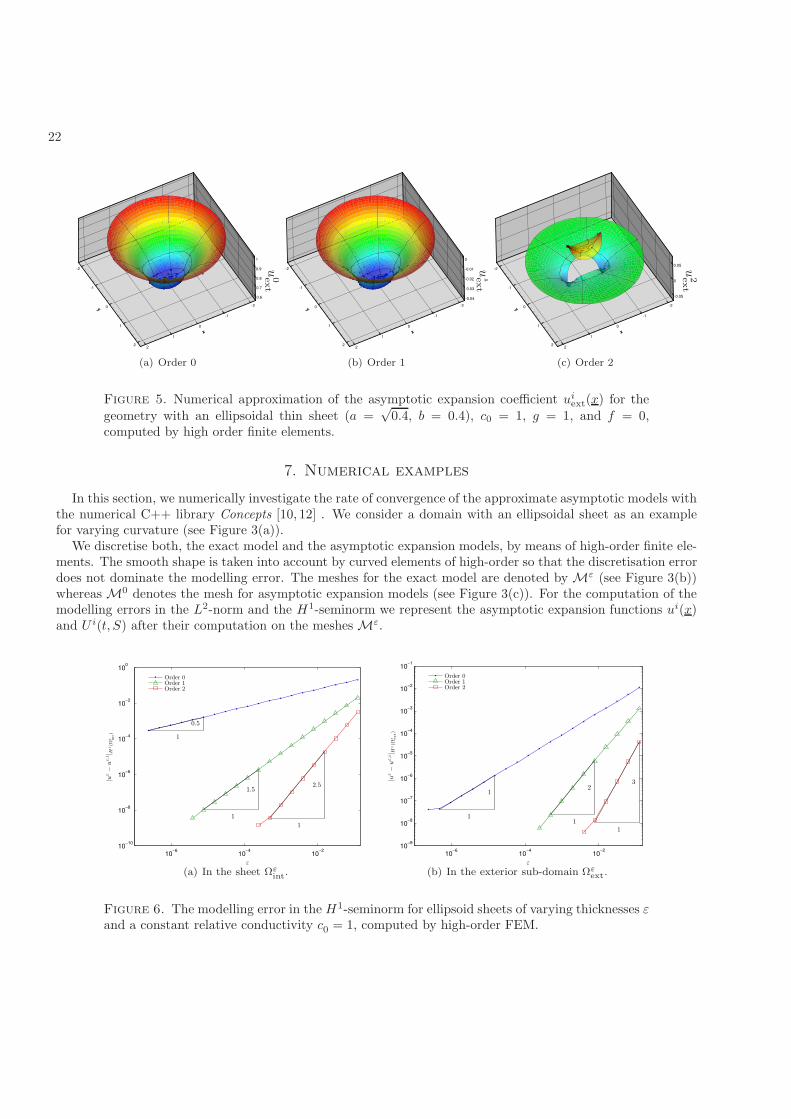
Figure 5. Numerical approximation of the asymptotic expansion coefficient uiext(x) for the
geometry with an ellipsoidal thin sheet (a =√
0.4, b = 0.4), c0 = 1, g = 1, and f = 0,computed by high order finite elements.
7. Numerical examples
In this section, we numerically investigate the rate of convergence of the approximate asymptotic models withthe numerical C++ library Concepts [10, 12] . We consider a domain with an ellipsoidal sheet as an examplefor varying curvature (see Figure 3(a)).
We discretise both, the exact model and the asymptotic expansion models, by means of high-order finite ele-ments. The smooth shape is taken into account by curved elements of high-order so that the discretisation errordoes not dominate the modelling error. The meshes for the exact model are denoted by Mε (see Figure 3(b))whereas M0 denotes the mesh for asymptotic expansion models (see Figure 3(c)). For the computation of themodelling errors in the L2-norm and the H1-seminorm we represent the asymptotic expansion functions ui(x)and U i(t, S) after their computation on the meshes Mε.
10−6
10−4
10−2
10−10
10−8
10−6
10−4
10−2
100
ε
|uε−
uε,i| H
1(Ω
ε int)
1
0.5
1
1.5
1
2.5
Order 0Order 1Order 2
(a) In the sheet Ωεint
.
10−6
10−4
10−2
10−9
10−8
10−7
10−6
10−5
10−4
10−3
10−2
10−1
ε
|uε−
uε,i| H
1(Ω
ε ext)
1
1
1
2
1
3
Order 0Order 1Order 2
(b) In the exterior sub-domain Ωεext.
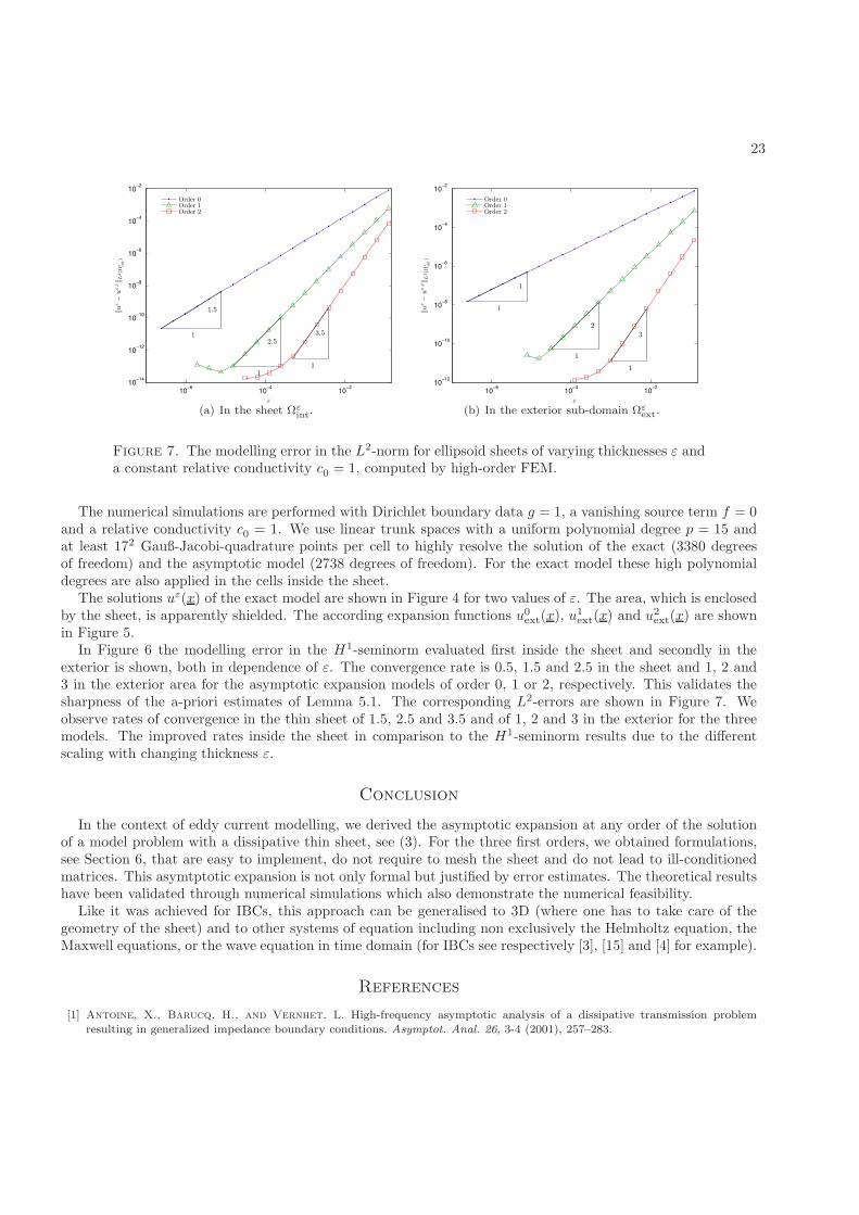
Figure 6. The modelling error in the H1-seminorm for ellipsoid sheets of varying thicknesses εand a constant relative conductivity c0 = 1, computed by high-order FEM.
23
10−6
10−4
10−2
10−14
10−12
10−10
10−8
10−6
10−4
10−2
ε
‖uε−
uε,i‖ L
2(Ω
ε int)
1
1.5
1
2.5
1
3.5
Order 0Order 1Order 2
(a) In the sheet Ωεint
.
10−6
10−4
10−2
10−12
10−10
10−8
10−6
10−4
10−2
ε
‖uε−
uε,i‖ L
2(Ω
ε int)
1
1
1
2
1
3
Order 0Order 1Order 2
(b) In the exterior sub-domain Ωεext.
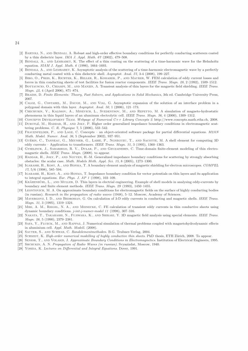
Figure 7. The modelling error in the L2-norm for ellipsoid sheets of varying thicknesses ε anda constant relative conductivity c0 = 1, computed by high-order FEM.
The numerical simulations are performed with Dirichlet boundary data g = 1, a vanishing source term f = 0and a relative conductivity c0 = 1. We use linear trunk spaces with a uniform polynomial degree p = 15 andat least 172 Gauß-Jacobi-quadrature points per cell to highly resolve the solution of the exact (3380 degreesof freedom) and the asymptotic model (2738 degrees of freedom). For the exact model these high polynomialdegrees are also applied in the cells inside the sheet.
The solutions uε(x) of the exact model are shown in Figure 4 for two values of ε. The area, which is enclosedby the sheet, is apparently shielded. The according expansion functions u0
ext(x), u1ext(x) and u2
ext(x) are shownin Figure 5.
In Figure 6 the modelling error in the H1-seminorm evaluated first inside the sheet and secondly in theexterior is shown, both in dependence of ε. The convergence rate is 0.5, 1.5 and 2.5 in the sheet and 1, 2 and3 in the exterior area for the asymptotic expansion models of order 0, 1 or 2, respectively. This validates thesharpness of the a-priori estimates of Lemma 5.1. The corresponding L2-errors are shown in Figure 7. Weobserve rates of convergence in the thin sheet of 1.5, 2.5 and 3.5 and of 1, 2 and 3 in the exterior for the threemodels. The improved rates inside the sheet in comparison to the H1-seminorm results due to the differentscaling with changing thickness ε.
Conclusion
In the context of eddy current modelling, we derived the asymptotic expansion at any order of the solutionof a model problem with a dissipative thin sheet, see (3). For the three first orders, we obtained formulations,see Section 6, that are easy to implement, do not require to mesh the sheet and do not lead to ill-conditionedmatrices. This asymtptotic expansion is not only formal but justified by error estimates. The theoretical resultshave been validated through numerical simulations which also demonstrate the numerical feasibility.
Like it was achieved for IBCs, this approach can be generalised to 3D (where one has to take care of thegeometry of the sheet) and to other systems of equation including non exclusively the Helmholtz equation, theMaxwell equations, or the wave equation in time domain (for IBCs see respectively [3], [15] and [4] for example).
References
[1] Antoine, X., Barucq, H., and Vernhet, L. High-frequency asymptotic analysis of a dissipative transmission problemresulting in generalized impedance boundary conditions. Asymptot. Anal. 26, 3-4 (2001), 257–283.
24
[2] Bartoli, N., and Bendali, A. Robust and high-order effective boundary conditions for perfectly conducting scatterers coatedby a thin dielectric layer. IMA J. Appl. Math. 67 (2002), 479–508.
[3] Bendali, A., and Lemrabet, K. The effect of a thin coating on the scattering of a time-harmonic wave for the Helmholtzequation. SIAM J. Appl. Math. 6 (1996), 1664–1693.
[4] Bendali, A., and Lemrabet, K. Asymptotic analysis of the scattering of a time-harmonic electromagnetic wave by a perfectlyconducting metal coated with a thin dielectric shell. Asymptot. Anal. 57, 3-4 (2008), 199–227.
[5] Biro, O., Preis, K., Richter, K., Heller, R., Komarek, P., and Maurer, W. FEM calculation of eddy current losses andforces in thin conducting sheets of test facilities for fusion reactor components. IEEE Trans. Magn. 28, 2 (1992), 1509–1512.
[6] Bottauscio, O., Chiampi, M., and Manzin, A. Transient analysis of thin layers for the magnetic field shielding. IEEE Trans.Magn. 42, 4 (April 2006), 871–874.
[7] Braess, D. Finite Elements: Theory, Fast Solvers, and Applications in Solid Mechanics, 3th ed. Cambridge University Press,2007.
[8] Caloz, G., Costabel, M., Dauge, M., and Vial, G. Asymptotic expansion of the solution of an interface problem in apolygonal domain with thin layer. Asymptot. Anal. 50, 1 (2006), 121–173.
[9] Chechurin, V., Kalimov, A., Minevich, L., Svedentsov, M., and Repetto, M. A simulation of magneto-hydrostaticphenomena in thin liquid layers of an aluminum electrolytic cell. IEEE Trans. Magn. 36, 4 (2000), 1309–1312.
[10] Concepts Development Team. Webpage of Numerical C++ Library Concepts 2. http://www.concepts.math.ethz.ch, 2008.[11] Durufle, M., Haddar, H., and Joly, P. Higher order generalized impedance boundary conditions in electromagnetic scat-
tering problems. C. R. Physique 7, 5 (2006), 533–542.[12] Frauenfelder, P., and Lage, C. Concepts – an object-oriented software package for partial differential equations. M2AN
Math. Model. Numer. Anal. 36, 5 (September 2002), 937–951.[13] Guerin, C., Tanneau, G., Meunier, G., Labie, P., Ngnegueu, T., and Sacotte, M. A shell element for computing 3D
eddy currents – Application to transformers. IEEE Trans. Magn. 31, 3 (1995), 1360–1363.[14] Gyselinck, J., Sabariego, R. V., Dular, P., and Geuzainehin, C. Time-domain finite-element modeling of thin electro-
magnetic shells. IEEE Trans. Magn. (2008). to appear.[15] Haddar, H., Joly, P., and Nguyen, H.-M. Generalized impedance boundary conditions for scattering by strongly absorbing
obstacles: the scalar case. Math. Models Meth. Appl. Sci. 15, 8 (2005), 1273–1300.[16] Igarashi, H., Kost, A., and Honma, T. A boundary element analysis of magnetic shielding for electron microscopes. COMPEL
17, 5/6 (1998), 585–594.[17] Igarashi, H., Kost, A., and Honma, T. Impedance boundary condition for vector potentials on thin layers and its application
to integral equations. Eur. Phys. J. AP 1 (1998), 103–109.[18] Krahenbuhl, L., and Muller, D. Thin layers in electrial engineering. Example of shell models in analysing eddy-currents by
boundary and finite element methods. IEEE Trans. Magn. 29 (1993), 1450–1455.[19] Leontovich, M. A. On approximate boundary conditions for electromagnetic fields on the surface of highly conducting bodies
(in russian). Research in the propagation of radio waves (1948), 5–12. Moscow, Academy of Sciences.[20] Mayergoyz, I. D., and Bedrosian, G. On calculation of 3-D eddy currents in conducting and magnetic shells. IEEE Trans.
Magn. 31, 3 (1995), 1319–1324.[21] Miri, A. M., Riegel, N. A., and Meinecke, C. FE calculation of transient eddy currents in thin conductive sheets using
dynamic boundary conditions. j-int-j-numer-model 11 (1998), 307–316.[22] Nakata, T., Takahashi, N., Fujiwara, K., and Shiraki, Y. 3D magnetic field analysis using special elements. IEEE Trans.
Magn. 26, 5 (1990), 2379–2381.[23] Safa, Y., Flueck, M., and Rappaz, J. Numerical simulation of thermal problems coupled with magnetohydrodynamic effects
in aluminium cell. Appl. Math. Modell. (2008).[24] Sauter, S., and Schwab, C. Randelementmethoden. B.G. Teubner-Verlag, 2004.[25] Schmidt, K. High-order numerical modelling of highly conductive thin sheets. PhD thesis, ETH Zurich, 2008. To appear.[26] Senior, T., and Volakis, J. Approximate Boundary Conditions in Electromagnetics. Institution of Electrical Engineers, 1995.[27] Shchukin, A. N. Propagation of Radio Waves (in russian). Svyazizdat, Moscow, 1940.[28] Yosida, K. Lectures on Differential and Integral Equations. Dover, 1991.
Research Reports
No. Authors Title
08-28 K.Schmidt, S. Tordeux Asymptotic modelling of conductive thinsheets
08-27 R. Hiptmair, P.R. Kotiuga,S. Tordeux
Self-adjoint curl operators
08-26 N. Reich Wavelet compression of anisotropic integro-differential operators on sparse tensor prod-uct spaces
08-25 N. Reich Anisotropic operator symbols arising frommultivariate jump processes
08-24 N. Reich Wavelet compression of integral operatorson sparse tensor spaces: Construction,Consistency and Asymptotically OptimalComplexity
08-23 F. Liu, N. Reich andA. Zhou
Two-scale finite element discretizations for in-finitesimal generators of jump processes infinance
08-22 M. Bieri and Ch. Schwab Sparse high order FEM for elliptic sPDEs
08-21 M. Torrilhon andR. Jeltsch
Essentially optimal explicit Runge-Kuttamethods with application to hyperbolic-parabolic equations
08-20 G. Dahlquist andR. Jeltsch
Generalized disks of contractivity for explicitand implicit Runge-Kutta methods
08-19 M. Karow and D. Kressner On the structured distance to uncontroll-ability
08-18 D. Kressner,Ch. Schroeder andD.S. Watkins
Implicit QR algorithms for palindromic andeven eigenvalue problems
08-17 B. Kagstroem, D. Kressner,E.S. Quintana-Ort andG. Quintana-Ort
Blocked algorithms for the reduction toHessenberg-Triangular form revisited
08-16 R. Granat, B. Kagstroemand D. Kressner
Parallel eigenvalue reordering in real Schurforms
08-15 P. Huguenot, H. Kumar,V. Wheatley, R. Jeltsch,C. Schwab andM. Torrilhon
Numerical simulations of high current arc incircuit breakers