Agricultural and Biosystems EngineeringConference Proceedings and Presentations Agricultural and Biosystems Engineering

2016

Development of an Autonomous IndoorPhenotyping RobotDylan ShahIowa State University

Lie TangIowa State University, lietang@iastate.edu

Follow this and additional works at: https://lib.dr.iastate.edu/abe_eng_conf

Part of the Agriculture Commons, and the Bioresource and Agricultural Engineering Commons

The complete bibliographic information for this item can be found at https://lib.dr.iastate.edu/abe_eng_conf/565. For information on how to cite this item, please visit http://lib.dr.iastate.edu/howtocite.html.

This Conference Proceeding is brought to you for free and open access by the Agricultural and Biosystems Engineering at Iowa State University DigitalRepository. It has been accepted for inclusion in Agricultural and Biosystems Engineering Conference Proceedings and Presentations by an authorizedadministrator of Iowa State University Digital Repository. For more information, please contact digirep@iastate.edu.

Development of an Autonomous Indoor Phenotyping Robot

AbstractIn order to fully understand the interaction between phenotype and genotype x environment to improve cropperformance, a large amount of phenotypic data is needed. Studying plants of a given strain under multipleenvironments can greatly help to reveal their interactions. To collect the labor-intensive data required toperform experiments in this area, an indoor rover has been developed, which can accurately andautonomously move between and inside growth chambers. The system uses mecanum wheels, magnetic tapeguidance, a Universal Robots UR 10 robot manipulator, and a Microsoft Kinect v2 3D sensor to positionvarious sensors in this constrained environment. Integration of the motor controllers, robot arm, and aMicrosoft Kinect (v2) 3D sensor was achieved in a customized C++ program. Detecting and segmentingplants in a multi-plant environment is a challenging task, which can be aided by integration of depth data intothese algorithms. Image-processing functions were implemented to filter the depth image to minimize noiseand remove undesired surfaces, reducing the memory requirement and allowing the plant to be reconstructedat a higher resolution in real-time. Three-dimensional meshes representing plants inside the chamber werereconstructed using the Kinect SDK’s KinectFusion. After transforming user-selected points in cameracoordinates to robot-arm coordinates, the robot arm is used in conjunction with the rover to probe desiredleaves, simulating the future use of sensors such as a fluorimeter and Raman spectrometer. This paper showsthe system architecture and some preliminary results of the system, as tested using a life-sized growth chambermock-up. A comparison of using raw camera coordinates data and using KinectFusion data is presented. Theresults suggest that the KinectFusion pose estimation is fairly accurate, only decreasing accuracy by a fewmillimeters at distances of roughly 0.8 meter.

Keywordsgrowth chambers, mechatronics, robotics, software development

DisciplinesAgriculture | Bioresource and Agricultural Engineering

CommentsThis proceeding is published as Shah, Dylan S., and Lie Tang. "Development of an Autonomous IndoorPhenotyping Robot." ASABE Annual International Meeting, Orlando, FL, July 17-20, 2016. Paper No.162460767. DOI: 10.13031/aim.20162460767. Posted with permission.

This conference proceeding is available at Iowa State University Digital Repository: https://lib.dr.iastate.edu/abe_eng_conf/565

ASABE Annual International Meeting 1

1

An ASABE Meeting Presentation DOI: 10.13031/aim.20162460767 Paper Number: 162460767

Development of an Autonomous Indoor Phenotyping Robot

Dylan Shah1, Lie Tang1

Iowa State University, Agricultural and Biosystems Engineering Department. Ames, IA, 50011, USA.

Written for presentation at the 2016 ASABE Annual International Meeting

Sponsored by ASABE Orlando, Florida July 17-20, 2016

ABSTRACT. In order to fully understand the interaction between phenotype and genotype x environment to improve crop performance, a large amount of phenotypic data is needed. Studying plants of a given strain under multiple environments can greatly help to reveal their interactions. To collect the labor-intensive data required to perform experiments in this area, an indoor rover has been developed, which can accurately and autonomously move between and inside growth chambers. The system uses mecanum wheels, magnetic tape guidance, a Universal Robots UR 10 robot manipulator, and a Microsoft Kinect v2 3D sensor to position various sensors in this constrained environment. Integration of the motor controllers, robot arm, and a Microsoft Kinect (v2) 3D sensor was achieved in a customized C++ program. Detecting and segmenting plants in a multi-plant environment is a challenging task, which can be aided by integration of depth data into these algorithms. Image-processing functions were implemented to filter the depth image to minimize noise and remove undesired surfaces, reducing the memory requirement and allowing the plant to be reconstructed at a higher resolution in real-time. Three-dimensional meshes representing plants inside the chamber were reconstructed using the Kinect SDK’s KinectFusion. After transforming user-selected points in camera coordinates to robot-arm coordinates, the robot arm is used in conjunction with the rover to probe desired leaves, simulating the future use of sensors such as a fluorimeter and Raman spectrometer. This paper shows the system architecture and some preliminary results of the system, as tested using a life-sized growth chamber mock-up. A comparison of using raw camera coordinates data and using KinectFusion data is presented. The results suggest that the KinectFusion pose estimation is fairly accurate, only decreasing accuracy by a few millimeters at distances of roughly 0.8 meter. Keywords. growth chambers, mechatronics, robotics, software development

The authors are solely responsible for the content of this meeting presentation. The presentation does not necessarily reflect the official position of the American Society of Agricultural and Biological Engineers (ASABE), and its printing and distribution does not constitute an endorsement of views which may be expressed. Meeting presentations are not subject to the formal peer review process by ASABE editorial committees; therefore, they are not to be presented as refereed publications. Citation of this work should state that it is from an ASABE meeting paper. EXAMPLE: Author’s Last Name, Initials. 2016. Title of presentation. ASABE Paper No. ---. St. Joseph, MI.: ASABE. For information about securing permission to reprint or reproduce a meeting presentation, please contact ASABE at http://www.asabe.org/copyright (2950 Niles Road, St. Joseph, MI 49085-9659 USA).1

ASABE Annual International Meeting Page 2

Introduction In a world of changing climate and increasing world population, there is a great need to understand the interaction

between genotype and phenotype in order to produce enough crop yield. Organizations such as the Royal Society of London (2009) and the FAO (Rai, et al., 2011) suggest a need for at least a 50% increase in food supply in the next half-century. This will not be achieved without a drastic change in the way we grow our food. Sustainable intensification, involving increasing the productivity of existing farmland while reducing negative environmental impacts, is promoted as one of the best ways – and some would say the only way - to achieve this.

One of the main methods to increase crop yield without increasing chemical use involves plant breeding techniques. Effective plant breeding requires in-depth data on plants’ health and growth patterns, which are part of their broader phenotype, or physical characteristics. Many traits relating to growth, performance, and yield are complex traits under polygenic control (Pieruschka & Poorter, 2012). Studying these traits using plants’ phenotypes to understand how each strain behaves under various growing conditions is an important step toward improving the characteristics of a crop stock. This paper presents a technical solution to several issues relating to current phenotyping techniques.

Due to the large amount of manual labor required in traditional by-hand phenotyping methods, numerous studies and experiments have been exploring phenotyping methods that are based on images, often either RGB (red, green, and blue channels) or RGB-D (red, green, blue, and depth channels). For instance, one phenotyping technique uses infrared and depth images acquired with a CamCube ToF camera (Alenya, Dellen, Foix, & Torras, 2013). The method involves taking a general view of the plant, segmenting to find leaves which are suitable for probing, and then moving the cameras closer to the suitable leaf using a Barret WAM arm. This leaf is then probed with a sample cutting tool. This points to the possibility for an application of a wide variety of sensors. For instance, fluorescence imaging sensors could be placed on the end of the robot arm for investigating the fluorochrome chlorophyll, which is involved in crop yield (Chaerle & Van Der Straeten, 2001). Numerous other sensors, such as near-infrared spectroscopy, can be applied to extract phenotypic data (Montes, Melchinger, & Reif, 2007).

Other image-based phenotyping techniques use infrared stereo image sequences to extract depth and then segment the resulting data to extract parameters such as leaf area and number of leaves (Aksoy, et al., 2015). Tobacco plants can be stereo-imaged periodically, using a KUKA robot arm. The image pairs are then run through an OpenCV block-matching algorithm to extract depth information. Next, the images are segmented to distinguish each leaf. Leaf area is found by ellipse-fitting each leaf, and the number of leaves is compared to the ground truth obtained via human measurement. Since these methods used fixed plant imaging positions, the methods are mainly suitable for stationary plants and a stationary robot arm, limiting the experiment to one growth environment. In a growing area larger than the reach of the robot arm, this approach also requires conveyance of the plants out of their growth environment, introducing other stress factors outside of the designed environment. Azzari et al. (2013) fused several point clouds, sometimes as many as 2000 point clouds per plant, to reconstruct the plant for extraction several pieces of information, including volume and allometric relationships. Point clouds were attained through manually moving their first-generation Kinect (v1). Chaivivatrakul et al. (2014) fused several point clouds into one 3d reconstruction and then extracted traits of corn plants such as leaf area, leaf length, and stem diameter. This method didn’t consider the case where multiple plants are in view. Finally, phenotyping can also be done in the field (Klodt, 2015). By taking a pair of images of the same grapevine plant, on several different days, some phenotyping can be done automatically. Once image pairs are acquired, they can be rectified to extract depth information, and finally segmented to find leaf and stem areas. This method did not provide an automated image capturing technique, and did not provide a framework for integration with other sensors for monitoring plant growth.

The solution presented in this paper required a minimal amount of labor during run-time, and can be extended, by adapting established phenotyping and plant-breeding to the techniques, to track plants that are growing in multiple growth environments concurrently. This solution involved an autonomous rover equipped with a Universal Robots UR 10 (UR10) robot arm, an industrial computer, a Microsoft Kinect (v2) sensor, and a rover base. The system was self-powered and required no wires to the outside world. The rover was equipped with a 120V power supply capable of powering numerous auxiliary sensors. This system allows for attachment of plant monitoring equipment, as illustrated in two small proof-of-concept experiments. In the first, the rover autonomously moved to the region representing the desired growth chamber in a setup mimicking Iowa State University’s future Enviratron plant growth facility. This facility will contain several growth chambers with a robot vestibule in front of each chamber door. Once at the destination, the system probed several plants in the chamber with a rigidly-mounted steel rod that simulates other sensors that need to be placed at a certain distance and with a specific orientation to plant leaves. In the second experiment, the robot probed leaves on one plant using three related but different data sources, to compare the accuracy of each source.

ASABE Annual International Meeting Page 3

THE PHYSICAL SYSTEM

Background on Hardware and Design

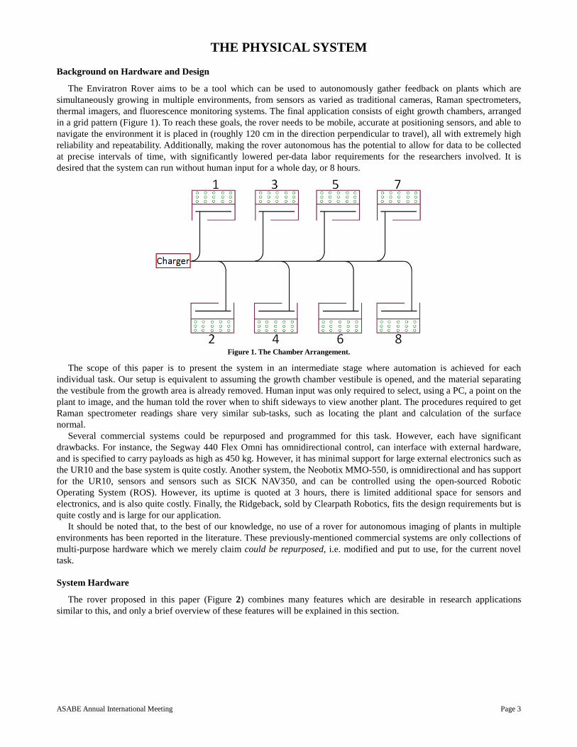
The Enviratron Rover aims to be a tool which can be used to autonomously gather feedback on plants which are simultaneously growing in multiple environments, from sensors as varied as traditional cameras, Raman spectrometers, thermal imagers, and fluorescence monitoring systems. The final application consists of eight growth chambers, arranged in a grid pattern (Figure 1). To reach these goals, the rover needs to be mobile, accurate at positioning sensors, and able to navigate the environment it is placed in (roughly 120 cm in the direction perpendicular to travel), all with extremely high reliability and repeatability. Additionally, making the rover autonomous has the potential to allow for data to be collected at precise intervals of time, with significantly lowered per-data labor requirements for the researchers involved. It is desired that the system can run without human input for a whole day, or 8 hours.

Figure 1. The Chamber Arrangement.

The scope of this paper is to present the system in an intermediate stage where automation is achieved for each individual task. Our setup is equivalent to assuming the growth chamber vestibule is opened, and the material separating the vestibule from the growth area is already removed. Human input was only required to select, using a PC, a point on the plant to image, and the human told the rover when to shift sideways to view another plant. The procedures required to get Raman spectrometer readings share very similar sub-tasks, such as locating the plant and calculation of the surface normal.

Several commercial systems could be repurposed and programmed for this task. However, each have significant drawbacks. For instance, the Segway 440 Flex Omni has omnidirectional control, can interface with external hardware, and is specified to carry payloads as high as 450 kg. However, it has minimal support for large external electronics such as the UR10 and the base system is quite costly. Another system, the Neobotix MMO-550, is omnidirectional and has support for the UR10, sensors and sensors such as SICK NAV350, and can be controlled using the open-sourced Robotic Operating System (ROS). However, its uptime is quoted at 3 hours, there is limited additional space for sensors and electronics, and is also quite costly. Finally, the Ridgeback, sold by Clearpath Robotics, fits the design requirements but is quite costly and is large for our application.

It should be noted that, to the best of our knowledge, no use of a rover for autonomous imaging of plants in multiple environments has been reported in the literature. These previously-mentioned commercial systems are only collections of multi-purpose hardware which we merely claim could be repurposed, i.e. modified and put to use, for the current novel task.

System Hardware

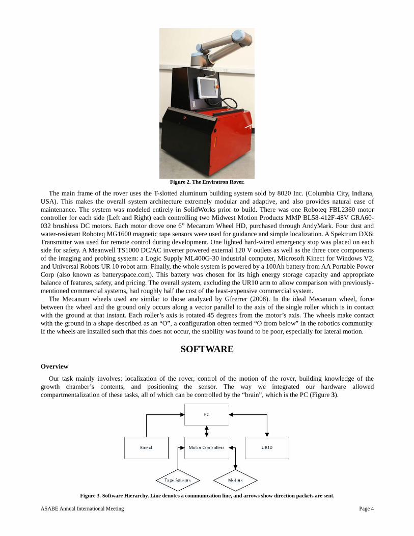
The rover proposed in this paper (Figure 2) combines many features which are desirable in research applications similar to this, and only a brief overview of these features will be explained in this section.

ASABE Annual International Meeting Page 4

Figure 2. The Enviratron Rover.

The main frame of the rover uses the T-slotted aluminum building system sold by 8020 Inc. (Columbia City, Indiana, USA). This makes the overall system architecture extremely modular and adaptive, and also provides natural ease of maintenance. The system was modeled entirely in SolidWorks prior to build. There was one Roboteq FBL2360 motor controller for each side (Left and Right) each controlling two Midwest Motion Products MMP BL58-412F-48V GRA60-032 brushless DC motors. Each motor drove one 6” Mecanum Wheel HD, purchased through AndyMark. Four dust and water-resistant Roboteq MG1600 magnetic tape sensors were used for guidance and simple localization. A Spektrum DX6i Transmitter was used for remote control during development. One lighted hard-wired emergency stop was placed on each side for safety. A Meanwell TS1000 DC/AC inverter powered external 120 V outlets as well as the three core components of the imaging and probing system: a Logic Supply ML400G-30 industrial computer, Microsoft Kinect for Windows V2, and Universal Robots UR 10 robot arm. Finally, the whole system is powered by a 100Ah battery from AA Portable Power Corp (also known as batteryspace.com). This battery was chosen for its high energy storage capacity and appropriate balance of features, safety, and pricing. The overall system, excluding the UR10 arm to allow comparison with previously-mentioned commercial systems, had roughly half the cost of the least-expensive commercial system.

The Mecanum wheels used are similar to those analyzed by Gfrerrer (2008). In the ideal Mecanum wheel, force between the wheel and the ground only occurs along a vector parallel to the axis of the single roller which is in contact with the ground at that instant. Each roller’s axis is rotated 45 degrees from the motor’s axis. The wheels make contact with the ground in a shape described as an “O”, a configuration often termed “O from below” in the robotics community. If the wheels are installed such that this does not occur, the stability was found to be poor, especially for lateral motion.

SOFTWARE

Overview

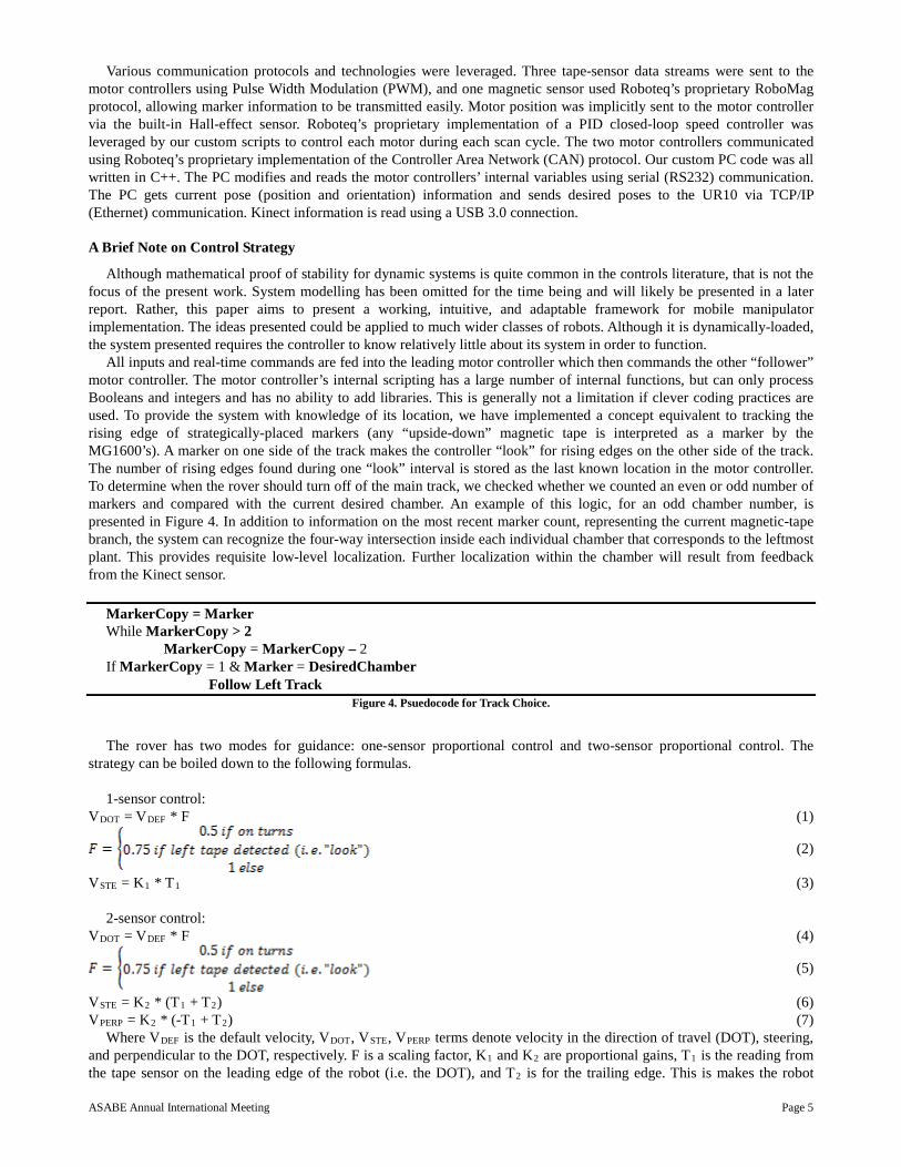
Our task mainly involves: localization of the rover, control of the motion of the rover, building knowledge of the growth chamber’s contents, and positioning the sensor. The way we integrated our hardware allowed compartmentalization of these tasks, all of which can be controlled by the “brain”, which is the PC (Figure 3).

Figure 3. Software Hierarchy. Line denotes a communication line, and arrows show direction packets are sent.

ASABE Annual International Meeting Page 5

Various communication protocols and technologies were leveraged. Three tape-sensor data streams were sent to the motor controllers using Pulse Width Modulation (PWM), and one magnetic sensor used Roboteq’s proprietary RoboMag protocol, allowing marker information to be transmitted easily. Motor position was implicitly sent to the motor controller via the built-in Hall-effect sensor. Roboteq’s proprietary implementation of a PID closed-loop speed controller was leveraged by our custom scripts to control each motor during each scan cycle. The two motor controllers communicated using Roboteq’s proprietary implementation of the Controller Area Network (CAN) protocol. Our custom PC code was all written in C++. The PC modifies and reads the motor controllers’ internal variables using serial (RS232) communication. The PC gets current pose (position and orientation) information and sends desired poses to the UR10 via TCP/IP (Ethernet) communication. Kinect information is read using a USB 3.0 connection.

A Brief Note on Control Strategy

Although mathematical proof of stability for dynamic systems is quite common in the controls literature, that is not the focus of the present work. System modelling has been omitted for the time being and will likely be presented in a later report. Rather, this paper aims to present a working, intuitive, and adaptable framework for mobile manipulator implementation. The ideas presented could be applied to much wider classes of robots. Although it is dynamically-loaded, the system presented requires the controller to know relatively little about its system in order to function.

All inputs and real-time commands are fed into the leading motor controller which then commands the other “follower” motor controller. The motor controller’s internal scripting has a large number of internal functions, but can only process Booleans and integers and has no ability to add libraries. This is generally not a limitation if clever coding practices are used. To provide the system with knowledge of its location, we have implemented a concept equivalent to tracking the rising edge of strategically-placed markers (any “upside-down” magnetic tape is interpreted as a marker by the MG1600’s). A marker on one side of the track makes the controller “look” for rising edges on the other side of the track. The number of rising edges found during one “look” interval is stored as the last known location in the motor controller. To determine when the rover should turn off of the main track, we checked whether we counted an even or odd number of markers and compared with the current desired chamber. An example of this logic, for an odd chamber number, is presented in Figure 4. In addition to information on the most recent marker count, representing the current magnetic-tape branch, the system can recognize the four-way intersection inside each individual chamber that corresponds to the leftmost plant. This provides requisite low-level localization. Further localization within the chamber will result from feedback from the Kinect sensor.

MarkerCopy = Marker While MarkerCopy > 2 MarkerCopy = MarkerCopy – 2 If MarkerCopy = 1 & Marker = DesiredChamber Follow Left Track

Figure 4. Psuedocode for Track Choice.

The rover has two modes for guidance: one-sensor proportional control and two-sensor proportional control. The

strategy can be boiled down to the following formulas. 1-sensor control:

VDOT = VDEF * F (1)

(2)

VSTE = K1 * T1 (3) 2-sensor control:

VDOT = VDEF * F (4)

(5)

VSTE = K2 * (T1 + T2) (6) VPERP = K2 * (-T1 + T2) (7)

Where VDEF is the default velocity, VDOT, VSTE, VPERP terms denote velocity in the direction of travel (DOT), steering, and perpendicular to the DOT, respectively. F is a scaling factor, K1 and K2 are proportional gains, T1 is the reading from the tape sensor on the leading edge of the robot (i.e. the DOT), and T2 is for the trailing edge. This is makes the robot

ASABE Annual International Meeting Page 6

correct the difference in the Tape readings by moving perpendicular to DOT; if the robot is moved forward both sensors will read opposite signs and strengthen the feedback. Similarly, an improperly-oriented robot, i.e. one that is not “pointing along the track”, will have both sensors have the same sign and the steer command will be strengthened. The three velocity terms are summed appropriately for each wheel (c.f. AndyMark), and the results are sent to the individual motors.

Pre-Processing of Kinect Depth Data

The imaging and probing system has to be inherently robust to varying leaf size, stalk height, and plant type. Two approaches have been considered: 1) the trivial case of hard-coding robot-arm positions to several generally-desired poses, such as “front view” and “top view”. 2) The general case of calculating desired pose based on knowledge of the sensor being used and the current arrangement of plants. For this study, we focused on the second, more general case.

Researchers have proposed using many 3D reconstruction methods on plants including structured light (Nguyen, et al., 2015), time of flight (ToF) (Alenyá, 2013), and stereo reconstruction (Biskup, 2007). The Kinect V2 sensor was chosen for this study due to its affordable price, useful features and specifications (c.f., Butkiewicz 2014), and well-documented application program interface (API). An additional advantage of the Kinect V2 is that its Software Development Kit (SDK) provides reasonably accurate reconstruction sample code, termed KinectFusion, that integrates easily into custom applications (Izadi et al., 2011, and Microsoft, 2016).

Feeding an unfiltered depth image to the KinectFusion algorithm was found to lead to a gradual erosion of the leaves, stalk, and stems of the plant, resulting in unusable meshes. However, this off-the-shelf algorithm was found to be very effective if an appropriately-filtered depth image was instead passed to the algorithm. The number of voxels that are tracked are limited, and unstable voxels are filtered out, to allow the algorithm to run in real time. In our application the table and walls surrounding the plant are far more stable than the pixels corresponding to the thin-stemmed, thin-leaved plants.

We wanted an algorithm that was computationally efficient enough to allow quick reconstructions, and knew the Kinect V2 API has an accurate mapping between the color camera and the depth camera. However, not every depth pixel has a corresponding color pixel due to physical properties of the sensors. We set depth pixels without an RGB counterpart to zero. Incoming images from the Kinect were put into a data structure that is effectively an RGB image. This representation is known to be sensitive to lighting changes, and there are methods for dealing with this issue. Luckily, however, the Kinect V2 had quite effective auto-brightness capabilities so lighting changes weren’t a significant issue. The challenge was finding an appropriate color space that allowed for easy identification of plant matter. Yang and Waibel, for instance, found that human faces were clustered in what they term chromatic color space (Yang 1997). We are mainly interested in plants, which are generally diffuse green and brown objects, so we chose to convert our RGB input image into HSV. After conversion to HSV, an experimentally-determined threshold was applied to each depth pixel. Let Dij (Tij) represent the pixel in row i row and column j of the R x C depth image (thresholded depth image), corresponding to a region of the HSV image as determined by the Kinect API’s mapping. We have, for ,

(10)

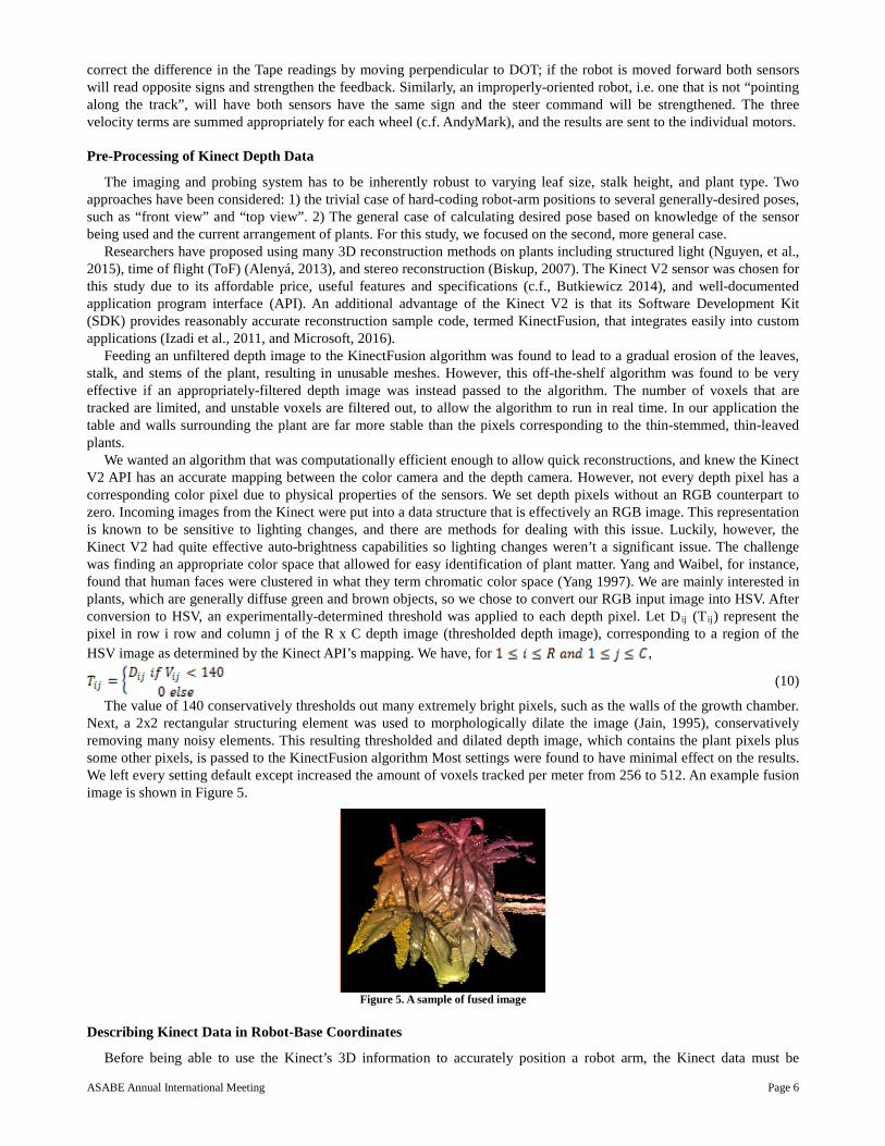
The value of 140 conservatively thresholds out many extremely bright pixels, such as the walls of the growth chamber. Next, a 2x2 rectangular structuring element was used to morphologically dilate the image (Jain, 1995), conservatively removing many noisy elements. This resulting thresholded and dilated depth image, which contains the plant pixels plus some other pixels, is passed to the KinectFusion algorithm Most settings were found to have minimal effect on the results. We left every setting default except increased the amount of voxels tracked per meter from 256 to 512. An example fusion image is shown in Figure 5.

Figure 5. A sample of fused image

Describing Kinect Data in Robot-Base Coordinates

Before being able to use the Kinect’s 3D information to accurately position a robot arm, the Kinect data must be

ASABE Annual International Meeting Page 7

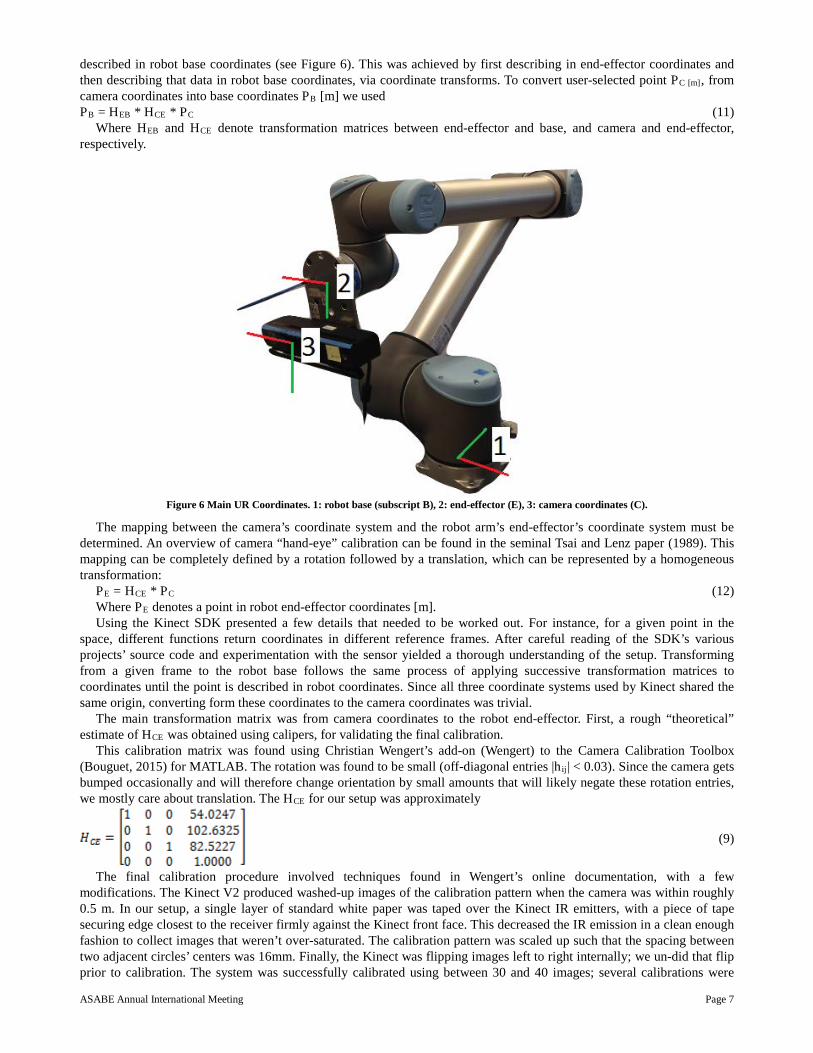
described in robot base coordinates (see Figure 6). This was achieved by first describing in end-effector coordinates and then describing that data in robot base coordinates, via coordinate transforms. To convert user-selected point PC [m], from camera coordinates into base coordinates PB [m] we used PB = HEB * HCE * PC (11)

Where HEB and HCE denote transformation matrices between end-effector and base, and camera and end-effector, respectively.

Figure 6 Main UR Coordinates. 1: robot base (subscript B), 2: end-effector (E), 3: camera coordinates (C).

The mapping between the camera’s coordinate system and the robot arm’s end-effector’s coordinate system must be determined. An overview of camera “hand-eye” calibration can be found in the seminal Tsai and Lenz paper (1989). This mapping can be completely defined by a rotation followed by a translation, which can be represented by a homogeneous transformation:

PE = HCE * PC (12) Where PE denotes a point in robot end-effector coordinates [m]. Using the Kinect SDK presented a few details that needed to be worked out. For instance, for a given point in the

space, different functions return coordinates in different reference frames. After careful reading of the SDK’s various projects’ source code and experimentation with the sensor yielded a thorough understanding of the setup. Transforming from a given frame to the robot base follows the same process of applying successive transformation matrices to coordinates until the point is described in robot coordinates. Since all three coordinate systems used by Kinect shared the same origin, converting form these coordinates to the camera coordinates was trivial.

The main transformation matrix was from camera coordinates to the robot end-effector. First, a rough “theoretical” estimate of HCE was obtained using calipers, for validating the final calibration.

This calibration matrix was found using Christian Wengert’s add-on (Wengert) to the Camera Calibration Toolbox (Bouguet, 2015) for MATLAB. The rotation was found to be small (off-diagonal entries |hij | < 0.03). Since the camera gets bumped occasionally and will therefore change orientation by small amounts that will likely negate these rotation entries, we mostly care about translation. The HCE for our setup was approximately

(9)

The final calibration procedure involved techniques found in Wengert’s online documentation, with a few modifications. The Kinect V2 produced washed-up images of the calibration pattern when the camera was within roughly 0.5 m. In our setup, a single layer of standard white paper was taped over the Kinect IR emitters, with a piece of tape securing edge closest to the receiver firmly against the Kinect front face. This decreased the IR emission in a clean enough fashion to collect images that weren’t over-saturated. The calibration pattern was scaled up such that the spacing between two adjacent circles’ centers was 16mm. Finally, the Kinect was flipping images left to right internally; we un-did that flip prior to calibration. The system was successfully calibrated using between 30 and 40 images; several calibrations were

ASABE Annual International Meeting Page 8

performed to perfect the process. Doing rapid calibration enables the end system to be modified to accommodate additional sensors without delaying the rest of the experiments’ schedule significantly.

After the points are described in end-effector coordinates, we desire to describe them in robot base coordinates. Given a

pose of the robot, defined by position and rotation vector in the robot base coordinates, we desire the transformation matrix from the end effector to the base. This is given by

(11)

Where . And the rotation matrix R is defined as

(12) Where c = cos(θ), s = sin(θ) and v = 1-cos(θ). See Craig (2009) for discussion. In the experiment presented in this paper, described later, all coordinates were transformed to “camera” coordinates

immediately after their variable’s initialization. The pose used for HEB depended on where the data was obtained from, as explained later.

Obtaining Position and Normal

To aid in planning for the next phase of the project, three different methods of probing were implemented. All three used the same Kinect camera and the same probing algorithm. However, the source of the normal and position information was different.

The Kinect for Windows SDK (K4W) has functions for mapping between the color frame (RGB) to the camera space (“K2”). Using OpenCV, K4W, and custom methods (functions), the first method involved using the Kinect’s internally-estimated, real-time position and normal of the internal KinectFusion mesh point corresponding to an RGB point clicked on our OpenCV window. The pose of the robot at the initialization of that instance of KinectFusion was used to calculate HEB, since data is returned after being transformed to initial-pose “camera coordinates” using Kinect’s estimate of the current pose relative to the initial pose. Part of our future work includes redoing the experiment with an exact transformation matrix, as obtained using matrix algebra on the HEB matrices based on the UR10’s pose feedback.

The second method used three points in the Kinect’s real-time depth space corresponding to RGB points. The point clicked on our OpenCV window gave us the desired position. The surface normal was obtained using the K4W CameraSpace coordinates associated with the clicked pixel (p1), a pixel five pixels to the right (p2); since the RGB images are flipped this is equivalent to -x in camera coordinates), and a pixel five pixels below (p3) in the RGB image. The pose used to calculate HEB was the pose of the robot at the instant the probing button was clicked. This data is real-time, and not dependent on the estimated relative pose. The surface normal was the cross product of the vector from p1 to p2 and the vector from p1 to p3. Quantitatively: V1 = p2 - p1, V2 = p3 - p1, and N = V1 × V2. V1 and V2 are vectors.

The third method involved manually opening the mesh generated by KinectFusion with the software Meshlab and saving the coordinates of three points (minimum necessary to understand the leaf’s normal and position), to .txt files. Logic used to find the normal in this third method was the same as in the “second method” above. This data uses the same HEB as method 1.

For methods 1 and 2, the user simply clicked the desired point and clicked probe. In method 3, there was roughly a minute of required interaction between the user and the PC, per probe. In future more-autonomous systems, we propose using traditional RGB image processing methods to detect the desired leaf location, rather than having the user interact with the system. Again, the goal is to develop this robotic system until it is fully autonomous for an entire day.

Calculating Desired Robot Pose

Next, we calculated the desired end-effector coordinate system axes AX, AY, AZ. Two logical constraints were added to our system. Az should align with the surface normal N and the Kinect should be level with the ground. Since our probe end-effector is orthogonal to our end-effector’s XY plane, i.e., it extends in the Az direction, we solved the following equations for AX, Ay and AZ: Az = -N, Ax ∙ N = 0, Axz = 0, and Ay = Az × Ax (13 a,b,c,d)

This can be solved by two directions of Ax. To disambiguate, two checks were implemented. First, if AY is pointing up and the normal is not pointing high, rotate 180 degrees so AY is downward. Else, if AX points left, rotate 180 degrees so the Kinect doesn’t hit the plant.

The position the end-effector moved to, p1, is a translation from the actual leaf position. Our probe stick was offset from the tool center point in the direction of the tool’s x-axis, and was orthogonal to the tool’s XY plane. Thus, the end-effector position, in robot base coordinates, was defined by:

ASABE Annual International Meeting Page 9

(14) Where L is the length of the probe stick and r = radius from the tool center point to the thin probe. Next, we determined

the rotation vector to send to the arm by solving equation 12 for rx, ry, and rz. Finally, the calculated coordinate values were sent to the UR10 to probe the leaf.

EXPERIMENTS This section presents two experiments. The first uses the rover to position the UR10 appropriately, and uses method 3

(“Text file” method) to probe two plants. The second experiment uses a stationary rover to position the UR10 appropriately, and uses all three described probing methods to probe one plant. For all probing’s, the goal location was the bottom-left corner, from the perspective of the crouched robot, of a small piece of painters’ tape, roughly 5mm square. For easy identification, one leaf had two additional pieces placed away from the goal location, and one leaf had one additional piece.

Mobile Rover

This section presents an experiment demonstrating current effectiveness of the proposed system. The UR 10 arm was commanded to probe two plants (one artificial Silk Dracaena plant - VCK8023, from artificialplantsandtrees.com - and one real Ficus plant), on three separate leaves, five times each (i.e. 30 separate probing’s). Both plants were placed on a 73 cm-high table (roughly the height that the UR base is at), around 1m apart. During normal conditions, the UR arm would extend roughly 80 centimeters in its Y direction for its end-effector to hit a desired leaf.

Before each trial, the rover was set up at the edge of a track with complete magnetic tape as would be in a setup with one chamber. The rover entered the “chamber” and stopped at the intersection. A user clicked a button on the PC’s custom user interface (UI), commanding the rover to shift sideways. There was only one issue with the tape-following navigation. After trial 3, one sensor reported magnetic tape in an un-taped portion of concrete. The sensors were calibrated with the Roboteq utility and the experiment proceeded as planned. As the lab currently lacks access to a 2D robot-tracking setup, the precision of this tape-following is omitted for this report.

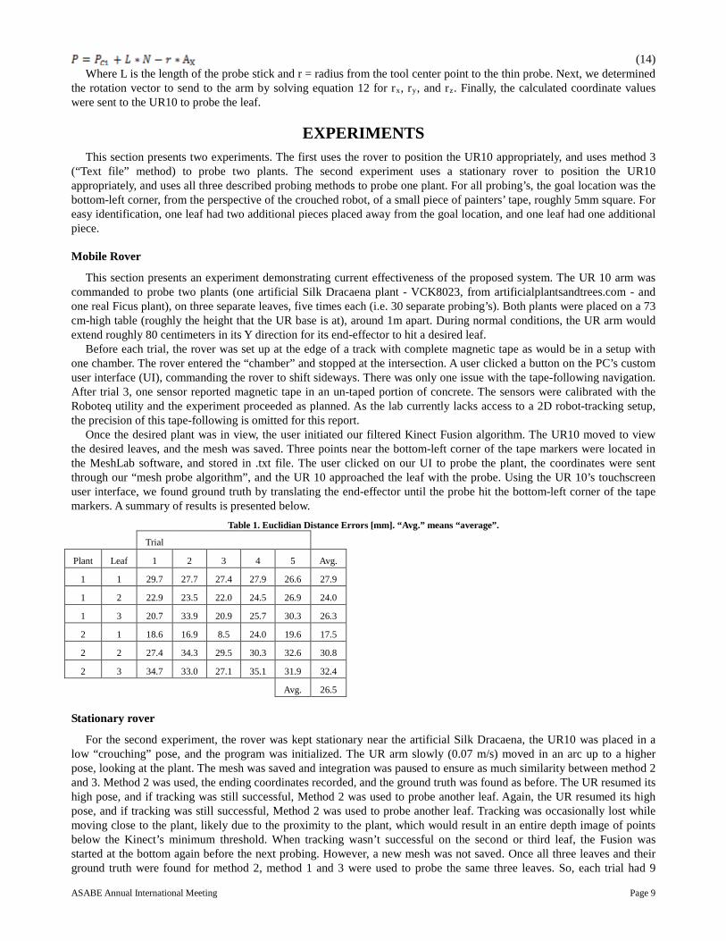
Once the desired plant was in view, the user initiated our filtered Kinect Fusion algorithm. The UR10 moved to view the desired leaves, and the mesh was saved. Three points near the bottom-left corner of the tape markers were located in the MeshLab software, and stored in .txt file. The user clicked on our UI to probe the plant, the coordinates were sent through our “mesh probe algorithm”, and the UR 10 approached the leaf with the probe. Using the UR 10’s touchscreen user interface, we found ground truth by translating the end-effector until the probe hit the bottom-left corner of the tape markers. A summary of results is presented below.

Table 1. Euclidian Distance Errors [mm]. “Avg.” means “average”.

Trial

Plant Leaf 1 2 3 4 5 Avg.

1 1 29.7 27.7 27.4 27.9 26.6 27.9

1 2 22.9 23.5 22.0 24.5 26.9 24.0

1 3 20.7 33.9 20.9 25.7 30.3 26.3

2 1 18.6 16.9 8.5 24.0 19.6 17.5

2 2 27.4 34.3 29.5 30.3 32.6 30.8

2 3 34.7 33.0 27.1 35.1 31.9 32.4

Avg. 26.5

Stationary rover

For the second experiment, the rover was kept stationary near the artificial Silk Dracaena, the UR10 was placed in a low “crouching” pose, and the program was initialized. The UR arm slowly (0.07 m/s) moved in an arc up to a higher pose, looking at the plant. The mesh was saved and integration was paused to ensure as much similarity between method 2 and 3. Method 2 was used, the ending coordinates recorded, and the ground truth was found as before. The UR resumed its high pose, and if tracking was still successful, Method 2 was used to probe another leaf. Again, the UR resumed its high pose, and if tracking was still successful, Method 2 was used to probe another leaf. Tracking was occasionally lost while moving close to the plant, likely due to the proximity to the plant, which would result in an entire depth image of points below the Kinect’s minimum threshold. When tracking wasn’t successful on the second or third leaf, the Fusion was started at the bottom again before the next probing. However, a new mesh was not saved. Once all three leaves and their ground truth were found for method 2, method 1 and 3 were used to probe the same three leaves. So, each trial had 9

ASABE Annual International Meeting Page 10

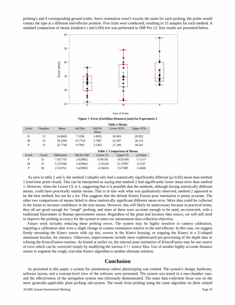
probing’s and 9 corresponding ground truths. Since orientation wasn’t exactly the same for each probing, the probe would contact the tape at a different end-effector position. Five trials were conducted, resulting in 15 samples for each method. A standard comparison of means (student’s t and LSD) test was performed in JMP Pro 12. Key results are presented below.

10

20

30

40

50

60

D M P

Type of Probe Figure 7. Error (Euclidian Distance) [mm] for Experiment 2

Table 2 Means Level Number Mean Std Dev Std Err

Mean Lower 95% Upper 95%

D 15 24.8626 7.3296 1.8925 20.804 28.922 M 15 30.2206 10.7153 2.7667 24.287 36.155 P 15 32.7744 9.7993 2.5302 27.348 38.201

Table 3. Comparison of Means Level - Level Difference Std Err Dif Lower CL Upper CL p-Value

P D 7.911710 3.429062 0.99158 14.83184 0.0260* M D 5.357948 3.429062 -1.56218 12.27807 0.1257 P M 2.553762 3.429062 -4.36636 9.47389 0.4606 As seen in table 2 and 3, the method 2 (depth) only had a statistically significantly different (p<0.05) mean than method

1 (real-time point cloud). This can be interpreted as saying that method 2 had significantly lower mean error than method 1. However, when the Lower CL is 1, suggesting that it is possible that the methods, although having statistically different means, could have practically similar means. This is in line with what was qualitatively observed; method 2 appeared to be the best method, but not by a lot. This suggests that the default Kinect Fusion pose estimation is pretty accurate. The other two comparisons of means failed to show statistically significant different mean error. More data could be collected in the future to increase confidence in the true means. However, this will likely be unnecessary because in practical terms, they all are good enough for “rough” probing, and none of them were accurate enough to be used, un-corrected, with a traditional fluorimeter or Raman spectrometer sensor. Regardless of the plant leaf location data source, we will still need to improve the probing accuracy for the system to meet our autonomous data-collection objective.

Future work includes reducing these probing errors. The system may be highly sensitive to camera calibration, requiring a calibration after even a slight change in camera orientation relative to the end-effector. In this case, we suggest firmly mounting the Kinect sensor with zip ties, screws in the Kinect housing, or trapping the Kinect in a U-shaped aluminum bracket, for instance. Otherwise, improvements include more sophisticated pre-processing of the depth data or refining the KinectFusion routines. As hinted at earlier on, the internal pose estimation of KinectFusion may be one source of error which can be corrected simply by modifying the various C++ source files. Use of another highly accurate distance sensor to augment the rough, real-time Kinect algorithm is another alternate solution.

Conclusion As presented in this paper, a system for autonomous indoor phenotyping was created. The system’s design, hardware,

software layout, and a concept-level view of the software were presented. The system was tested in a one-chamber case, and the effectiveness of the navigation system was informally demonstrated. The main data-collection focus was on the more generally-applicable plant probing sub-system. The result from probing using the same algorithm on three related

ASABE Annual International Meeting Page 11

but different data structures were compared. Before installing other sensors, some refinement of the probing sub-system should be done, improving location accuracy. Additionally, the accuracy of surface normal estimation should be tested. As the final end-goal for our future work, we aim to make the system fully autonomous.

Acknowledgements

This material is based upon work supported by the National Science Foundation under Grant No. 1428148. The authors would like to thank Jingyao Gai and Rajesh Putta-Venkata for help during the early development of the probing algorithm, and undergraduate students Caleb Stafford, Taylor Wisgerhof, Layne Goertz, and Austin Plotz for help during the mechanical design phase.

Safety Emphasis In order to make the rover safe for interaction with humans, several features have been implemented. First, fuses were

inserted which minimizes risk of short-circuiting of contacts and risk of drawing current that is higher than components’ specifications. The battery consists of four sets of four 3.2.V (nominal) lithium-ion batteries (total 51.2 nominal). One fuse is inserted in between the 2 middle cell-sets, and one fuse is connected directly to the battery’s 48V contact. Both fuses are currently 25A. Secondly, one emergency stop, which cuts power to the motors, is on each side of the rover base. Third, the wheels are designed to have a “moderate” level of traction, so the rover is physically limited in its accelerations and in its ability to push objects. This reduces likelihood that the rover would trap someone against a wall, whether the robot or the human was at fault. Fourth, the robot arm is suitable for “Collaborative operation according to ISO 10218-1:2011” (Universal Robots, 2015). If the robot exceeds a safety setting (force, torque, velocity, etc.) the UR10 can go into a slow or stopped mode according to the user-defined settings.

Further internal electrical precautions were taken. High-current relays (arbitrarily chosen as 200A) implement the mergency-stop and main switch power control, allowing reliable operation. Some electrical precautions similar to those recommended in the motor controller manufacturer’s user manual (Roboteq) were implemented. These included a path from motor voltage terminal through a pull-down resistor to ground while the system is turned off (implemented using a five-pole single-throw industrial switch), and a path from the motor voltage terminal through a diode and a 10A fuse to the battery’s positive terminal to prevent over-voltage while the system is turned on. Finally, all significant wiring inside the controller has been sized appropriately, labelled, shielded with heat-shrinkable tubing and cable wrap, crimped with appropriately-rated wire crimps, and guided using cable ties and mounting pads. Bus bars were used to organize voltage contacts of the same voltage (24V, 48V, ground). This enhances maintenance and decreases the risk of electrical accidents. No unified standard was applied or monitored, however.

References Aksoy, E. E., Abramov, A., Wörgötter, F., Scharr, H., Fischbach, A., & Dellen, B. (2015). Modeling leaf growth of rosette plants using

infrared stereo image sequences. Computers and Electronics in Agriculture, 110, 78-90. Alenya, G., Dellen, B., Foix, S., & Torras, C. (2013). Robotized plant probing: leaf segmentation utilizing time-of-flight data. Robotics &

Automation Magazine, IEEE, 20(3), 50-59. AndyMark http://files.andymark.com/MecanumWheelSpecSheet.pdf Azzari, G., Goulden, M. L., & Rusu, R. B. (2013). Rapid characterization of vegetation structure with a Microsoft Kinect sensor. Sensors

(Basel, Switzerland), 13(2), 2384. Biskup, B., Scharr, H., Schurr, U., & Rascher, U. (2007). A stereo imaging system for measuring structural parameters of plant

canopies. Plant, Cell & Environment,30(10), 1299-1308. Bouguet, J.-Y. (2015). Camera calibration toolbox for MATLAB, http://www.vision.caltech.edu/bouguetj/calib_doc/ T. Butkiewicz, "Low-cost coastal mapping using Kinect v2 time-of-flight cameras," 2014 Oceans - St. John's, St. John's, NL, 2014, pp. 1-9. Chaerle, L., & Van Der Straeten, D. (2001). Seeing is believing: imaging techniques to monitor plant health. BBA - Gene Structure and

Expression, 1519(3), 153-166. Chaivivatrakul, S., Tang, L., Dailey, M. N., & Nakarmi, A. D. (2014). Automatic morphological trait characterization for corn plants via 3D

holographic reconstruction. Computers and Electronics in Agriculture, 109, 109-123. Corke, P., & Khatib, O. (2011). Robotics, Vision and Control Fundamental Algorithms in MATLAB®. Springer Berlin Heidelberg. Craig, J. J. (2005). Introduction to robotics : mechanics and control / John J. Craig (3rd ed.. ed.). Upper Saddle River, N.J.: Upper Saddle

River, N.J. : Pearson Education. Gfrerrer, A. (2008). Geometry and kinematics of the Mecanum wheel. Computer Aided Geometric Design, 25(9), 784-791. Izadi, S.; Kim, D.; Hilliges, O., Molynequx, D., Newcombe, R., Kohli, P. (2011). KinectFusion: real-rime 3D reconstruction and interaction

using a moving depth camera. In Proceedings of the 24th Annual ACM Symposium on User Interface Software and Technology. Jain, R., Kasturi, R., & Schunck, Brian G. (1995). Chapter 2: Binary Image Processing. In Machine vision / Ramesh Jain, Rangachar

Kasturi, Brian G. Schunck. New York: McGraw-Hill. Klodt, M., Herzog, K., Töpfer, R., & Cremers, D. (2015). Field phenotyping of grapevine growth using dense stereo reconstruction. BMC

ASABE Annual International Meeting Page 12

bioinformatics, 16, 143. Microsoft, (2016). Kinect Fusion: Kinect for Windows 1.7, 1.8. Microsoft.com. https://msdn.microsoft.com/en-us/library/dn188670.aspx Montes, J. M., Melchinger, A. E., & Reif, J. C. (2007). Novel throughput phenotyping platforms in plant genetic studies. Trends in Plant

Science, 12(10), 433-436. Nguyen, T. T., Slaughter, D. C., Max, N., Maloof, J. N., & Sinha, N. (2015). Structured light- Based 3D reconstruction System for Plants.

Sensors (Basel, Switzerland), 15(8), 18587. Pieruschka, R., & Poorter, H. (2012). Phenotyping plants: genes, phenes and machines. Functional Plant Biology, 39(11), 813-820. Rai, M., Reeves, T. G., Pandey, S., Collette, L., & Food and Agriculture Organization of the United, N. (2011). Save and grow : a

policymaker's guide to sustainable intensification of smallholder crop production / [final technical editing, Mangala Rai, Timothy Reeves and Shivaji Pandey ; lead authors: Linda Collette ... [et al.]]. Rome: Rome : Food and Agriculture Organization of the United Nations.

Robots, U. (2015). User Manual: UR10/CB3. Royal Society of London. (2009). Reaping the benefits: science and the sustainable intensification of global agriculture. Royal Society,

London. Tsai, R., & Lenz, R. (1989). A new technique for fully autonomous and efficient 3D robotics hand/eye calibration. Robotics and

Automation, IEEE Transactions on, 5(3), 345-358. Wengert, C. calib_toolbox_addon (Calibration Software)

http://www2.vision.ee.ethz.ch/software/calibration_toolbox//calibration_toolbox.php