Embed Size (px)
Citation preview
Pedro Miguel Botica Ferreira
Licenciado em Ciências de Engenharia Biomédica
Development of a web application for processingNeuroimaging data in the Cloud. Application to
Brain Connectivity
Dissertação para obtenção do Grau de Mestre em
Engenharia Biomédica
Orientador: Hugo Ferreira, Professor Auxiliar,Faculdade de Ciências da Universidade de Lisboa
Abril, 2017

Development of a web application for processing Neuroimaging data in theCloud. Application to Brain Connectivity
Copyright © Pedro Miguel Botica Ferreira, Faculdade de Ciências e Tecnologia, Universi-
dade NOVA de Lisboa.
A Faculdade de Ciências e Tecnologia e a Universidade NOVA de Lisboa têm o direito,
perpétuo e sem limites geográficos, de arquivar e publicar esta dissertação através de
exemplares impressos reproduzidos em papel ou de forma digital, ou por qualquer outro
meio conhecido ou que venha a ser inventado, e de a divulgar através de repositórios
científicos e de admitir a sua cópia e distribuição com objetivos educacionais ou de inves-
tigação, não comerciais, desde que seja dado crédito ao autor e editor.
Este documento foi gerado utilizando o processador (pdf)LATEX, com base no template “novathesis” [1] desenvolvido no Dep. Informática da FCT-NOVA [2].[1] https://github.com/joaomlourenco/novathesis [2] http://www.di.fct.unl.pt


To all those displaced from their homesdue to the conflicts of other men.
To those who face death for a chance at a lifewithout fear, only to be seen as a burden.


Acknowledgements
Firstly, I must express appreciation for my thesis advisor prof. Hugo Ferreira both for
proposing an interesting and challenging thesis topic and for the help given throughout
the entire work process. Secondly, my thanks to Instituto de Biofísica e Engenharia
Biomédica (IBEB) for providing me with a workspace and allowing me to meet so many
amazing people.
After over 5 years, I feel a great deal of gratitude not only to FCT-NOVA but also to
the great minds I had the honour to meet along the way. My thanks go to prof. Mário
Secca, prof. Carla Quintão Pereira and so many others which have had an impact in my
academic journey and helped me see the world in new ways.
Of course none of it would have been possible without my family: my father, my
mother, my brother and my grandmother. Thank you for just everything. For allowing
me the possibility to take this path, for the confidence placed in me, for the uncondi-
tional support. Thank you for enabling me to make these choices and supporting me all
throughout. Thank you for the love you bear me and know it is returned. A special word
of appreciation for my godparents could not go unsaid. Thank you for being an integral
part of my life and my family, and to my godmother Paula for being a unwavering beacon
of happiness.
Beyond the education I received these past years, I have been fortunate enough to
meet amazing people who have been an integral part of not only my academic journey
but my personal life as well. One friend in particular started this journey with me, and
together we reach the finish line. José Trindade, thank you old chap. Others I met along
the way, each adding their own colour to this 5 year canvas: Pedro Torcato, Hugo Santos,
Filipe Valadas and many others. Thank you all for your friendship, for all the joy, the
laughs and even the stressful moments we shared. A shout out goes, of course, to my
friend all the way from Finland, Aleksi Sorvali. Kiitos paljon for coming to visit and for
hosting me in Finland.
The past year has been fraught with stress and despair, but even in these times I was
lucky to have good friends (even making new ones) who helped me in this final sprint,
both with good advice and even by laughing at my stupid jokes. Thank you all for the
lunches, the coffee trips and, in all, your friendship. And also for enduring me in my
endeavour to fill the whiteboard of the downstairs laboratory. Thank you Diogo Duarte,
Carolina Amorim, Daniela Godinho, Rita Monteiro and many many others. Furthermore,
vii

a special word of appreciation for Raquel Almeida is very much in order. Thank you for
your help and guidance throughout this whole year, for putting up with my idiosyncrasies
always with a smile and for helping me fill the lab with laughter and the whiteboard with
random drawings.
Last but most certainly not least, thank you Rita Ginja. Thank you for your unwaver-
ing support and for keeping me sane, for helping me face this challenge and never letting
obstacles bring me down. And thank you for being by my side for the entire length of
this 5-year journey.
viii
Abstract
Neuropsychiatric disorders, or mental disorders, have long been known to be a major
cause of burden to society and it is estimated that one in every four people worldwide
will be affected by one of these conditions during their lifetime. The diagnosis of these
conditions is based on a set of subjective criteria and on the experience of physicians
and is therefore highly prone to error. Alcohol Use Disorder (AUD) is one such disorder
with particularly devastating consequences to both individual and society, representing a
total of 5.1% of the global burden of disease and injury. As image classification methods
improve, reaching near-human capabilities, and research on brain physiology continues
to advance and allow us to better understand brain structure and function through novel
methods such as Brain Connectivity analysis, ingenious approaches to medical diagnosis
can be envisioned. Furthermore, as new technologies allow the world to be more con-
nected and less dependent on physical machinery, there is an interest in bringing this
vision to both healthcare and biomedical research, through technologies such as Cloud
computing.
This work focuses on the creation of an intuitive Cloud-based application which uses
the image classification algorithm Convolutional Neural Network (CNN). The applica-
tion would then be used to classify Electroencephalography data to diagnose AUD, in
particular using Brain Connectivity metrics.
The created application was successfully developed according to the objectives, prov-
ing to be simple to operate but effective in the use of the CNN algorithm. However, due
to the environment used, it showed high processing times which hamper the training
of CNN classifiers. Classification results, while not conclusive, show indication that the
employed metrics and methodology may be of use in the context of neuropsychiatric dis-
order diagnosis both in a research and clinical context in the future. Finally, discussion
and analysis of these results were performed so as to drive forward the research into this
methodology.
Keywords: Convolutional Neural Networks, Cloud Computing, Alcohol Use Disorder,
Machine Learning, Brain Connectivity
ix

Resumo
Os distúrbios neuropsiquiátricos são das enfermidades com maior impacto mundial,
estimando-se que afectem uma em cada quatro pessoas durante a sua vida. O diagnós-
tico destas doenças é baseado num conjunto de critérios subjectivos e na experiência do
profissional de saúde que o conduz, estando sujeito a erro humano. O alcoolismo, um
destes distúrbios, é particularmente devastador, sendo o consumo de álcool responsável
por 5.1% do impacto causado por todas as doenças. À medida que os métodos de classi-
ficação de imagem melhoram e a investigação na área da fisiologia cerebral nos permite
compreender o funcionamento do cérebro através de métodos inovadores de análise de
Conectividade Cerebral, novas metodologias de diagnóstico clínico podem ser concebi-
das. Além do mais, a passo com a forma como novas tecnologias interligam o mundo e
reduzem a dependência em maquinaria física, surge o interesse em trazer esta visão ao
cuidado médico e à investigação biomédica com tecnologias como computação em Cloud.
Este trabalho foca-se na criação de uma aplicação em Cloud que seja intuitiva e use o
algoritmo de classificação de imagem Redes Neuronais Convolucionais. Esta aplicação foi
usada para classificar dados electroencefalográficos de modo a diagnosticar alcoolismo
usando métricas de Conectividade Cerebral.
A aplicação foi criada de acordo com as especificações, sendo muito intuitiva mas
também eficiente no seu uso do algoritmo pretendido. No entanto, devido ao ambiente
no qual foi implementado, sofre de um tempo de processamento que dificulta o treino de
redes. Os resultados da classificação de dados, apesar de não serem conclusivos, mostram
indícios de que as métricas e metodologia usadas poderão ser aplicadas num contexto
clínico e em investigação científica. Finalmente, discussão e análise dos resultados foram
realizadas de forma a desvendar potenciais direcções futuras para este trabalho.
Palavras-chave: Redes Neuronais Convolucionais, Computação em Nuvem, Alcoolismo,
Aprendizagem Automática, Conectividade Cerebral
Por decisão pessoal, o autor do texto não escreve segundo o novo Acordo Ortográfico
xi

Contents
List of Figures xv
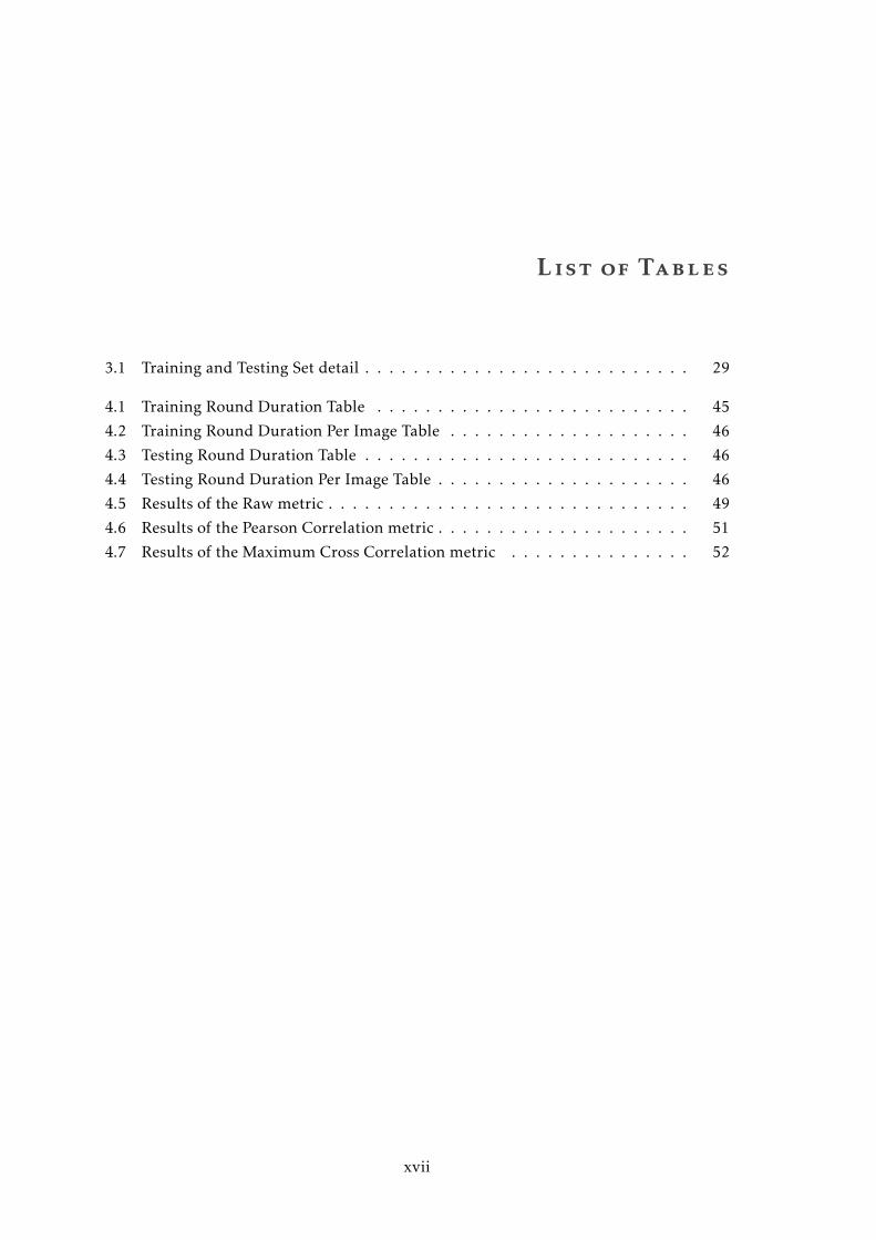
List of Tables xvii
Acronyms xix
1 Introduction 1
1.1 Context & Motivation . . . . . . . . . . . . . . . . . . . . . . . . . . . . . . 1
1.2 Objectives . . . . . . . . . . . . . . . . . . . . . . . . . . . . . . . . . . . . 5
1.3 Thesis Overview . . . . . . . . . . . . . . . . . . . . . . . . . . . . . . . . . 5
2 Theoretical Concepts 7
2.1 Alcohol Use Disorder . . . . . . . . . . . . . . . . . . . . . . . . . . . . . . 7
2.1.1 Definition & Pathophysiology . . . . . . . . . . . . . . . . . . . . . 7
2.1.2 Clinical Diagnosis . . . . . . . . . . . . . . . . . . . . . . . . . . . . 8
2.2 Electroencephalography . . . . . . . . . . . . . . . . . . . . . . . . . . . . 9
2.2.1 Introduction and Underlying Theory . . . . . . . . . . . . . . . . . 9
2.2.2 Analysis of Brain Connectivity . . . . . . . . . . . . . . . . . . . . 11
2.2.3 Brain Connectivity in Alcohol Use Disorder . . . . . . . . . . . . . 13
2.3 Machine Learning . . . . . . . . . . . . . . . . . . . . . . . . . . . . . . . . 14
2.3.1 Artificial Neural Networks . . . . . . . . . . . . . . . . . . . . . . . 14
2.3.2 Convolutional Neural Networks . . . . . . . . . . . . . . . . . . . . 15
2.4 Cloud Computing . . . . . . . . . . . . . . . . . . . . . . . . . . . . . . . . 22
2.4.1 Definition . . . . . . . . . . . . . . . . . . . . . . . . . . . . . . . . 22
2.4.2 Deployment Models . . . . . . . . . . . . . . . . . . . . . . . . . . 23
2.4.3 Cloud Service Models . . . . . . . . . . . . . . . . . . . . . . . . . . 23
3 Materials & Methods 25
3.1 Application . . . . . . . . . . . . . . . . . . . . . . . . . . . . . . . . . . . . 25
3.1.1 Theano© framework . . . . . . . . . . . . . . . . . . . . . . . . . . 25
3.1.2 Microsoft Azure® . . . . . . . . . . . . . . . . . . . . . . . . . . . . 26
3.1.3 Flask© Microframework . . . . . . . . . . . . . . . . . . . . . . . . 26
3.2 Classification . . . . . . . . . . . . . . . . . . . . . . . . . . . . . . . . . . . 27
xiii
CONTENTS
3.2.1 Datasets . . . . . . . . . . . . . . . . . . . . . . . . . . . . . . . . . 27
3.2.2 Image Creation Methodology . . . . . . . . . . . . . . . . . . . . . 29
3.2.3 Network Training Configuration . . . . . . . . . . . . . . . . . . . 32
3.2.4 Cross-Validation . . . . . . . . . . . . . . . . . . . . . . . . . . . . . 32
4 Results & Discussion 33
4.1 Application . . . . . . . . . . . . . . . . . . . . . . . . . . . . . . . . . . . . 33
4.1.1 Interface . . . . . . . . . . . . . . . . . . . . . . . . . . . . . . . . . 33
4.1.2 Structure . . . . . . . . . . . . . . . . . . . . . . . . . . . . . . . . . 34
4.1.3 Network Creation and Training . . . . . . . . . . . . . . . . . . . . 35
4.1.4 Data classification with an existing network . . . . . . . . . . . . . 38
4.1.5 Custom Network Architecture . . . . . . . . . . . . . . . . . . . . . 41
4.1.6 Data Labelling . . . . . . . . . . . . . . . . . . . . . . . . . . . . . . 43
4.1.7 Use of Theano . . . . . . . . . . . . . . . . . . . . . . . . . . . . . . 43
4.1.8 Cloud Environment . . . . . . . . . . . . . . . . . . . . . . . . . . . 43
4.1.9 Processing Time . . . . . . . . . . . . . . . . . . . . . . . . . . . . . 44
4.2 Classification . . . . . . . . . . . . . . . . . . . . . . . . . . . . . . . . . . . 48
4.2.1 MNIST Data . . . . . . . . . . . . . . . . . . . . . . . . . . . . . . . 48
4.2.2 Raw Data . . . . . . . . . . . . . . . . . . . . . . . . . . . . . . . . . 49
4.2.3 Pearson Correlation . . . . . . . . . . . . . . . . . . . . . . . . . . . 50
4.2.4 Maximum Cross-Correlation . . . . . . . . . . . . . . . . . . . . . . 51
4.2.5 Paradigm Comparison . . . . . . . . . . . . . . . . . . . . . . . . . 53
4.2.6 Metric Comparison . . . . . . . . . . . . . . . . . . . . . . . . . . . 54
5 Conclusions 57
5.1 Limitations . . . . . . . . . . . . . . . . . . . . . . . . . . . . . . . . . . . . 57
5.2 Future Work . . . . . . . . . . . . . . . . . . . . . . . . . . . . . . . . . . . 57
5.3 Final Thoughts . . . . . . . . . . . . . . . . . . . . . . . . . . . . . . . . . . 58
Bibliography 59
xiv
List of Figures
2.1 Modified Combinatorial Nomenclature of the International 10/20 System . . 10
2.2 Artificial Neuron Model . . . . . . . . . . . . . . . . . . . . . . . . . . . . . . 15
2.3 Three layered Artificial Neural Network Example . . . . . . . . . . . . . . . . 16
3.1 Example of an MNIST image . . . . . . . . . . . . . . . . . . . . . . . . . . . . 27
4.1 Website Main Page . . . . . . . . . . . . . . . . . . . . . . . . . . . . . . . . . . 34
4.2 Application Structure . . . . . . . . . . . . . . . . . . . . . . . . . . . . . . . . 35
4.3 Network Creation and Training Interface - Datasets Retrieval Prompt . . . . 36
4.4 Network Creation and Training Interface - Network Parameters . . . . . . . . 37
4.5 Network Creation and Training - Parameter Confirmation . . . . . . . . . . . 37
4.6 Network Training Interface . . . . . . . . . . . . . . . . . . . . . . . . . . . . . 38
4.7 Classification Page Interface . . . . . . . . . . . . . . . . . . . . . . . . . . . . 39
4.8 Network Loading Page Interface . . . . . . . . . . . . . . . . . . . . . . . . . . 39
4.9 Classification Results Interface . . . . . . . . . . . . . . . . . . . . . . . . . . 40
4.10 Caffe Network Upload Page Interface . . . . . . . . . . . . . . . . . . . . . . . 41
4.11 MNIST Classification Results . . . . . . . . . . . . . . . . . . . . . . . . . . . 48
4.12 Example of a Raw image . . . . . . . . . . . . . . . . . . . . . . . . . . . . . . 49
4.13 Example of a Pearson Correlation image . . . . . . . . . . . . . . . . . . . . . 50
4.14 Example of a Maximum Cross-Correlation image . . . . . . . . . . . . . . . . 51
4.15 Comparison of two Maximum Cross Correlation classification score plots dur-
ing training . . . . . . . . . . . . . . . . . . . . . . . . . . . . . . . . . . . . . . 53
xv

List of Tables
3.1 Training and Testing Set detail . . . . . . . . . . . . . . . . . . . . . . . . . . . 29
4.1 Training Round Duration Table . . . . . . . . . . . . . . . . . . . . . . . . . . 45
4.2 Training Round Duration Per Image Table . . . . . . . . . . . . . . . . . . . . 46
4.3 Testing Round Duration Table . . . . . . . . . . . . . . . . . . . . . . . . . . . 46
4.4 Testing Round Duration Per Image Table . . . . . . . . . . . . . . . . . . . . . 46
4.5 Results of the Raw metric . . . . . . . . . . . . . . . . . . . . . . . . . . . . . . 49
4.6 Results of the Pearson Correlation metric . . . . . . . . . . . . . . . . . . . . . 51
4.7 Results of the Maximum Cross Correlation metric . . . . . . . . . . . . . . . 52
xvii


Acronyms
ANN Artificial Neural Network.
AUD Alcohol Use Disorder.
BCI Brain-Computer Interface.
CNN Convolutional Neural Network.
CPU Central Processing Unit.
CSS Cascading Style Sheets.
ECG Electrocardiography.
EEG Electroencephalography.
fMRI Functional Magnetic Resonance Imaging.
GABA Gamma-aminobutyric Acid.
GPU Graphics Processing Unit.
HTML HyperText Markup Language.
IaaS Infrastructure-as-a-Service.
IBEB Instituto de Biofísica e Engenharia Biomédica.
MEG Magnetoencephalography.
xix
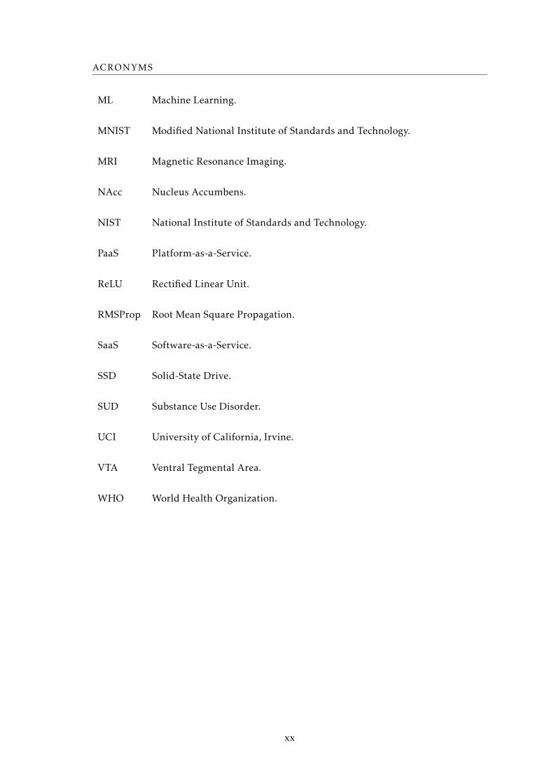
ACRONYMS
ML Machine Learning.
MNIST Modified National Institute of Standards and Technology.
MRI Magnetic Resonance Imaging.
NAcc Nucleus Accumbens.
NIST National Institute of Standards and Technology.
PaaS Platform-as-a-Service.
ReLU Rectified Linear Unit.
RMSProp Root Mean Square Propagation.
SaaS Software-as-a-Service.
SSD Solid-State Drive.
SUD Substance Use Disorder.
UCI University of California, Irvine.
VTA Ventral Tegmental Area.
WHO World Health Organization.
xx
Chapter
1Introduction
1.1 Context & Motivation
Neuropsychiatric disorders, or mental disorders, have an enormous impact on the world
population [1–11]. Though the prevalence of these conditions varies widely between
countries [12] it is estimated that, during their lifetime, one in every four people will be
affected by a mental disorder [11]. According to the World Health Organization (WHO),
these disorders are the most important causes of global illness-related burden, accounting
for around one third of years living with disability among adults [10].
Studies have shown that mental disorders represent approximately 40% of the medical
burden for young to middle-aged adults in North America [4] and that each year over one
third of the European Union population suffers from mental illness, with the prevalence
of disorders of the brain estimated to be much higher and representing the largest part
of total disease burden in these countries [8].
Although many neuropsychiatric disorders may not present physical disabilities [13],
all of these conditions greatly decrease quality of life as they progress [7], with symptoms
invariantly leading to an inability to function as the disease progresses without treatment
[5]. Moreover, these disorders tend to strike earlier in life and have a longer if not indefi-
nite duration when compared to other classes of pathologies such as infectious diseases
[5, 6]. Furthermore, the relative low importance most of these diseases are given in terms
of government funding, especially in developing countries, leads to a spread in the preva-
lence of these conditions, which then unavoidably increases their socio-economic burden
[5].
Psychiatric disorders become more debilitating as they go without treatment and pre-
vent bearers from being able to work and support themselves, often forcing this task
upon a caregiver [1–3, 5–8]. Caregivers are also often prevented from holding a job due
1
CHAPTER 1. INTRODUCTION
to the amount of burden placed upon them by the disease [5]. Studies have found that
caregivers often become depressed themselves, with caregiver burden for these condi-
tions far surpassing that of chronic diseases [1]. This demonstrates the toll psychiatric
disorders have upon society, as it has been shown that these conditions are among the
most burdensome not only to patients but also to caregivers and healthcare institutions
[1–8].
These conditions are also very frequently misdiagnosed, with currently employed
diagnostic methods suffering from subjectiveness and a high proneness to error [7, 14–
17]. Misdiagnosis of these conditions leads to a lack of proper treatment which itself
causes a worsening of symptoms [14–17].
Specifically alcoholism, formally defined as Alcohol Use Disorder (AUD), is a costly
and socially devastating mental disorder [13, 18–20]. Alcohol consumption degrades indi-
vidual health and heavily burdens society in terms of morbidity, mortality and disability
[18]. Alcohol is, in fact, one of the most commonly consumed addictive psychoactive
substances in the world [20], with its use being the cause of 5.9% of all world deaths (3.3
million per year) and a quarter of total deaths in the 20-39 year-old age group. Further-
more, its use brings significant economic and social losses not only to the individual but
to society as well, as 5.1% of the global burden of disease and injury is attributable to
alcohol consumption [19].
While nowadays research into the pathophysiology of neuropsychiatric diseases is con-
tinuously carried out, the mechanisms behind most of these conditions are still largely
unknown and being unravelled at a slow pace [21]. However, research using brain func-
tion analysis methods has shown that there is potential for a diagnosis application which
could be employed in a clinical context [21–25].
One of these methods relies on analysing the connections between different brain
structures from various perspectives [26]. Specifically studying the functional links that
exist in the brain, i.e. Functional Brain Connectivity Analysis, has proven to be an ef-
fective method in diagnosing and gauging the severity of brain-related disorders [25–
28].
Functional Brain Connectivity is, in fact, a widely studied concept as it can give
insight into how the brain’s neuron networks process information and how certain brain
processes are carried out [25–28].
Particularly, analysing Functional Brain Connectivity is a matter of data analysis and
has been applied to Functional Magnetic Resonance Imaging (fMRI), Electroencephalog-
raphy (EEG) and Magnetoencephalography (MEG) data using mathematical concepts that
allow the extraction of information regarding brain activity [26, 29]. EEG finds a use in
the analysis of Brain Connectivity and is of special interest in this context since its high
temporal resolution allows the study of the temporal dynamics of brain activity better
than other imaging techniques [29–33]. Notably, several neuropsychiatric disorders, in-
cluding AUD, have been found to show significant changes in functional connectivity and
this approach shows great promise in the study of these diseases [25–27, 34–36].
2

1.1. CONTEXT & MOTIVATION
While these methods allow to obtain large amounts of data, they mostly offer results
which may be complicated to subject to a direct human interpretation due to its high
dimensionality. Having a good metric which encodes brain activity that can be used in
diagnosis is of little value if result interpretation is difficult and may itself be subject to
human error. For that reason, Machine Learning (ML) algorithms are often employed
in these cases to offer not only automation but also to reduce subjectivity caused by
human interpretation, and may be needed in situations where a human view may not
fully encompass the full dimensionality of the data.
Besides its use in fields such as biometric recognition, gaming and marketing, ML has
also seen use in medicine, such as in decoding brain states through electrocortigraphic,
fMRI and scalp EEG data, with brain-computer interface technology being the driving
force for this advancement [37].
ML has, in fact, been used in a wide array of biomedical applications and has proven to
be a valuable tool in general healthcare [38], with notable uses including the classification
of electrocardiographic and auscultatory blood pressure to diagnose heart conditions
[39], identification of brain tumours from Magnetic Resonance Imaging (MRI) data [40],
extraction of metabolic markers [40], patient characterization [41], abnormality detection
in mammographies as aid to diagnosis [42], cancer prognosis and prediction [43] and in
the study of neuropsychiatric disorders [44].
Image processing is arguably the largest application of ML that has seen great advance-
ment in recent years [45]. With the development of modern medical imaging technologies,
the need for image classification programs increased tremendously and is today one of
the fastest growing fields of biomedical engineering [37].
Convolutional Neural Networks (CNNs), in particular, are one of the most advanced
types of ML algorithms and have been shown to achieve near-human performance ac-
curacies in image recognition tasks, and currently hold the best classification score of
the Modified National Institute of Standards and Technology (MNIST) database, with an
error rate of 0.21% [46]. CNNs find use in applications such as biometric identification
[45], programs that learn to replicate painters’ style [47], applications that extract high-
level human attributes such as gender and clothing [48], text classification [49], speech
recognition [50] and facial recognition [51]. It is also worth to note that Brain-Computer
Interface (BCI) is another field where the use of CNNs, in conjunction with EEG data, is
undergoing research and showing promise, with accuracy results reaching 95% in stim-
ulus response classification [52, 53]. Another relevant example of CNNs being used in
conjunction with EEG is in biometric recognition using resting-state EEG signals [54].
Healthcare applications of CNNs include classification of Alzheimer’s Disease pa-
tients from control subjects, reaching an accuracy result of 92% using EEG signal from
16 electrodes [55], segmentation of infant brain tissue in multi-modality MRI images [56]
and histological tissue classification [57]. CNNs have also been shown to achieve per-
formances comparable to expert radiologists in classifying radiological features (lumbar
inter-vertebral discs and vertebral bodies) from MRI images, with an accuracy of 95.6%
3
CHAPTER 1. INTRODUCTION
[58]. Finally, the use of CNNs has shown that applying pattern recognition to the spatio-
temporal dynamics of EEG with Brain Connectivity metrics can be used for epileptic
seizure prediction [59].
Other particularly relevant use of ML in healthcare research are the development of
an application to classify alcoholics and non-alcoholics using EEG and Neural Networks
[60] and another using several different EEG analysis metrics to classify alcoholic and
epileptic patients from control subjects and thus achieving accuracies of over 90% [36].
Another technology of interest that is growing in use is Cloud Computing [61–64].
This technology allows data and applications to be remotely housed and run in remote
servers while providing many advantages in terms of computational resource scalability
and pricing [61–63, 65, 66].
While the Cloud paradigm is not yet widely employed in healthcare mainly due to
some aspects regarding security that still need resolving, it poses as a growing area of
research in medicine and shows promise to change the way data is handled in healthcare
[61–64].
The Cloud paradigm allows for several users to have access to the same data, allow-
ing for the sharing of information among several healthcare entities such as physicians
or between institutions [61–63, 65, 66]. This means Cloud computing can be used in
Telemedicine both as an e-health data storage platform and as a data processing platform
and can even be useful in emergency situations due to easy and fast data access [61, 62].
Patient monitoring is another application of the Cloud paradigm as physicians can
access physiological data stored in the Cloud to remotely monitor test results or ongoing
therapies [63], with this concept having been studied through the use of Electrocardio-
graphy (ECG) data [64]. Using the same concept, Cloud systems can also be employed
in patient self-management as an easy way to keep track of medical information and
exam results [61, 62]. Also, using the Cloud paradigm as a way to outsource healthcare
facility records and for remote data processing has shown to save money otherwise spent
on hardware investment and maintenance costs. Medical imaging is another field where
healthcare can benefit from the use of Cloud servers due to their remote storage and
processing capabilities as medical images tend to be resource-heavy [63].
With all the information and studies presented above taken into consideration, an
application could be envisioned which makes use of ML concepts, in particular capitaliz-
ing on the strength of image processing algorithms such as CNN, and Brain Connectivity
analysis (with EEG) as a computer-aided diagnosis tool. Moreover, developing the ap-
plication in the Cloud would allow users to remotely access it and not be restricted by
the hardware available to them, as well as provide a cost-effective platform flexible to
continuous development.
AUD, being a highly prevalent mental disorder was chosen to be the subject of analysis
of the aforementioned application. Furthermore, studies presented above support the
notion that Brain Connectivity analysis of AUD is feasible to use in an automatic classifier
and that taking an Image Processing approach to the problem can give interesting results
4

1.2. OBJECTIVES
due to the advanced capabilities of these algorithms, in particular CNNs.
1.2 Objectives
This thesis can be seen as having two main objectives.
The first objective is to create an intuitive Cloud-based application which allows the
user to create, train and employ a specialized ML classifier.
The application is to follow a set of pre-determined core principles:
• Due to the current strength and wide use of image processing technologies, the
application must follow an image processing paradigm, where the input data to be
processed consists solely in images, and as such employs the CNN algorithm.
• To capitalize on modern Cloud-based technologies and the possibility of remote
processing and removal of physical hardware restraints, as well as the possibility
of more cost-effective deployments, the application is to be housed and run on a
Cloud server.
• To allow its use in research and an easily adaptability to different contexts, it must
be designed so that it is simple to learn and use.
The second objective is to employ the aforementioned application to classify neuropsy-
chiatric data and thus evaluate metrics which could be used to automatically classify
non-healthy subjects from control ones. A few core principles were also set in this second
objective:
• Due to advantages of EEG in terms of ease of use and superior temporal resolution,
it was chosen to be the type of physiological data acquisition to be used.
• Due to the fact that its diagnosis is less subjective and due to the relatively high
availability of data, the disorder to be used in this work was chosen to be Alcohol
Use Disorder.
1.3 Thesis Overview
The present chapter focuses on the background context of this thesis and explores how
these concepts serve as motivation for the work that will subsequently be discussed. The
main objectives are underlined as pertaining to the context and motivations discussed
previously. This is intended to give the reader a broad scope of the different issues
involved in this work and how each of them interconnect to give rise to what will be
discussed in later chapters.
The remainder of this thesis is segmented in such a way to promote a more fluid
reading:
5
CHAPTER 1. INTRODUCTION
• Chapter 2 presents the scientific concepts which were tackled in this work. A
great deal of focus was paid to CNN, as the development of the application and
analysis of results is greatly related to the intricacies of the algorithm. Furthermore,
the pathology of AUD was presented rather than neuropsychiatric disorders in
general. This is due to the fact that AUD is the only disorder in focus throughout this
work, though the research is embedded in the broader context of neuropsychiatric
disorders, as discussed in the present chapter.
• Chapter 3 is intended to introduce the tools used in this work. Here, a division is
made between those used in the context of application development and those used
in classification efforts. In the former, the computational tools such as programming
frameworks and the used Cloud environment are presented. In the latter, the used
datasets are detailed as thoroughly as possible. Data processing techniques and
classification parameters are also introduced.
• In Chapter 4, the developed application and classification results are presented and
discussed. Again, this chapter is divided such as to segment the created application
from the classification results so as to promote legibility. Both the application and
the classification results are analysed from different perspectives such that different
discussion topics arise and thus allowing a more complete analysis of the work and
not only an adequate evaluation of results but also the discovery of new directions
of research.
• Finally, in Chapter 5, the factors that posed obstacles to the performed research
are presented and discussed, followed by a contemplation of how the work can be
advanced in the future. To conclude, some final thoughts are shared in the interest
of bringing this thesis to a close.
6
Chapter
2Theoretical Concepts
2.1 Alcohol Use Disorder
2.1.1 Definition & Pathophysiology
Alcohol Use Disorder (AUD), more commonly known as alcoholism, is a kind of Sub-
stance Use Disorder (SUD) characterized by the excessive consumption of alcohol [13].
The main feature of these disorders is a set of behavioural, cognitive and physiological
phenomena showing the persistent use of the substance in spite of the problems it causes,
with substance use taking on a higher priority than other matters that once held much
greater importance [13, 67].
Other important features of these disorders lie in the set of symptoms experienced
when substance use is discontinued, known as withdrawal, and in the intense desire or
urge for the substance that may occur at any time, also known as craving [13].
Unlike other drugs of abuse, alcohol does not interact with a specific receptor or target
system in the brain but rather forms complex interactions with multiple neurotransmit-
ter/neuromodulator systems [68]. As such, the full scope of chemical brain processes
triggered in the presence of alcohol is not yet fully understood, though several neuro-
transmitter systems are known to be linked to alcohol dependence [67, 69, 70].
The activation of neurons in the brain is regulated by excitatory and inhibitory neu-
rotransmission processes. While, under normal conditions, a balance exists between
excitatory and inhibitory neurotransmitters in the brain, exposure to alcohol leads to
a state of imbalance. In this imbalance, inhibitory processes are intensified as alcohol
enhances the effect of inhibitory neurotransmitters, the main ones of these being Gamma-
aminobutyric Acid (GABA) and Glycine, as well as that of inhibitory neuromodulators,
such as Adenosine [71]. This causes a decrease in anxiety and an overall state of sedation
[67, 71].
7

CHAPTER 2. THEORETICAL CONCEPTS
It is this interaction with GABA, as well as other neurotransmitter systems and the
endogenous opioid system, that is thought to stimulate the release of dopamine from
cells in the Ventral Tegmental Area (VTA) to the limbic system, namely to the Nucleus
Accumbens (NAcc) and prefrontal cortex. This circuitry, also known as the brain’s reward
system, is associated with desire, motivation and reward-based learning and is thought to
play an important role in reinforcing evolutionary-beneficial behaviours. It is therefore
thought that this system plays an important role in developing addiction and is thought
to cause euphoria when consuming alcohol [68].
With long term exposure to alcohol, however, the brain begins to adapt by counterbal-
ancing its effects, in an attempt to restore equilibrium between excitatory and inhibitory
processes. As such, inhibitory neurotransmission is decreased and excitatory neurotrans-
mission is increased [71]. This state of compensated equilibrium is the mark of alcohol
dependence. It is important to realize that this shift in neurotransmission distribution is
only in equilibrium in the presence of alcohol. In the absence of alcohol, however, a new
state of reversed imbalance arises, leading to an increase in excitatory neurotransmission
and a decrease in inhibitory neurotransmission. This new unbalanced state is the basis of
withdrawal and causes symptoms such as seizures, delirium and anxiety and is character-
ized by an intense craving of alcohol as an attempt to restore neurotransmission balance
in the brain [71].
Heavy alcohol intake may lead to problems in nearly every organ system such as the
cardiovascular system (e.g. cardiomiopathy), the gastrointestinal tract (e.g. gastritis, liver
cirrhosis, pancreatitis), the skeletal system (e.g. osteoporosis, osteonecrosis) [13, 72] and
is known to affect most of the endochrine and neurochemical systems [18, 70]. Like other
SUDs, AUD has variable effects on the central and peripheral nervous systems and causes
aberrations in normal brain functions which, depending on the degree of addiction, may
not disappear after detoxification [13, 73]. Such effects include cognitive deficits, severe
memory impairment, and degenerative changes in the cerebellum [13].
2.1.2 Clinical Diagnosis
Diagnosis of AUD, or any SUD, is based on the pathological pattern of behaviours related
to substance use [13, 67]. There are eleven criteria to diagnose SUD, which can be grouped
into four categories [13]:
• impaired control
• social impairment
• risky use of the substance
• pharmacological criteria
8
2.2. ELECTROENCEPHALOGRAPHY
While analysis of urine or blood samples to measure blood alcohol concentration may
serve as evidence to confirm one or more criteria, diagnosis usually relies on asking ques-
tions regarding the subject’s experience with alcohol. To note that it is not required that it
be the subject to answer these questions, provided the answers come from reliable sources.
Besides diagnosing AUD, the number of confirmed criteria also allow a quantification of
the severity of the disorder, as the more criteria are verified, the higher the severity of the
disorder [13, 74].
Due to the fact that no empirical analysis is employed, this method of diagnosing
AUD and inferring its severity is considered subjective and frequent discussion arises
regarding its accuracy [74], especially when taking into consideration that the underlying
condition is highly heterogeneous in both etiology and phenotype [67]. This is common
to all neuropsychiatric disorders [13].
2.2 Electroencephalography
2.2.1 Introduction and Underlying Theory
Electroencephalography (EEG) is a technique that allows the collection of data pertaining
to the brain’s electrical activity [30, 75–77].
The neurons composing the brain work by moving charges to transmit information
to each other, in complex networks that encode brain function [30, 75, 76]. According
to Standard Electromagnetic Theory, a moving charge generates an electric field which
extends through space, decaying as distance to the charge increases. Thus, these small
currents generate electric fields which extend to the scalp. However, due to the small
magnitude of the currents produced by the activity of a single neuron, only the combined
simultaneous activity of several neurons can be detected as an electric potential at the
scalp [30, 75, 76]. As such, brain processes requiring the activity of a group of neurons
can be acquired and amplified for analysis [30, 77]. This is the basis of EEG.
Using electrodes with a conductive material allows for the resulting electric field at
the scalp to be read as an electric potential. This measurement can be stored and carried
out over time to acquire a dataset of varying electric potential at specific scalp regions.
The resulting data constitutes the EEG signal [30, 75–77].
Electrodes are placed in predetermined positions that depend on their amount and
in the used positioning system. The electrode number and configuration allows for the
customization of the acquisition parameters such as spatial resolution. The standard In-
ternational 10/20 electrode configuration is the most common but using more electrodes
involves using modified configurations to correctly place each one in the best position to
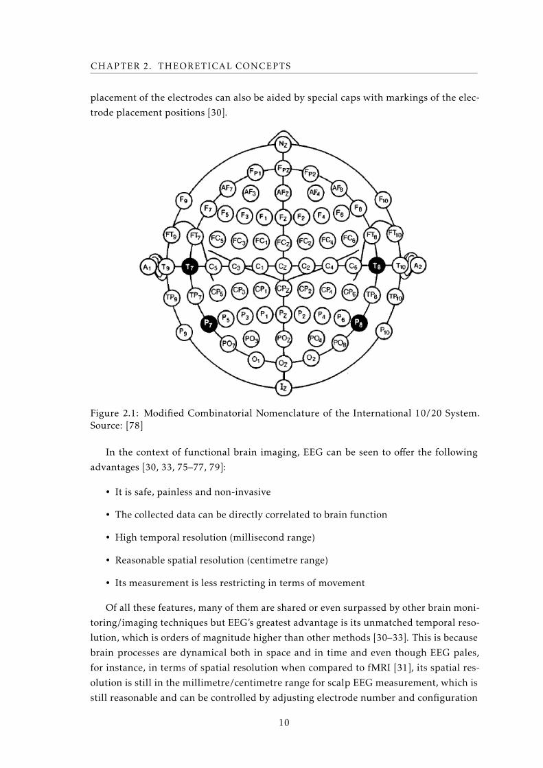
improve signal acquisition and reduce artefacts. Figure 2.1 shows the Modified Combi-
natorial Nomenclature, which features electrode positions from the International 10/20
System with a modification to designate the additional 10% electrode positions [78]. The
9
CHAPTER 2. THEORETICAL CONCEPTS
placement of the electrodes can also be aided by special caps with markings of the elec-
trode placement positions [30].
Figure 2.1: Modified Combinatorial Nomenclature of the International 10/20 System.Source: [78]
In the context of functional brain imaging, EEG can be seen to offer the following
advantages [30, 33, 75–77, 79]:
• It is safe, painless and non-invasive
• The collected data can be directly correlated to brain function
• High temporal resolution (millisecond range)
• Reasonable spatial resolution (centimetre range)
• Its measurement is less restricting in terms of movement
Of all these features, many of them are shared or even surpassed by other brain moni-
toring/imaging techniques but EEG’s greatest advantage is its unmatched temporal reso-
lution, which is orders of magnitude higher than other methods [30–33]. This is because
brain processes are dynamical both in space and in time and even though EEG pales,
for instance, in terms of spatial resolution when compared to fMRI [31], its spatial res-
olution is still in the millimetre/centimetre range for scalp EEG measurement, which is
still reasonable and can be controlled by adjusting electrode number and configuration
10
2.2. ELECTROENCEPHALOGRAPHY
[79]. Good temporal resolution, however, proves advantageous since capturing rapid
variations in neuron configurations is valuable in analysing brain function [30, 32, 33],
thus leading to the choice of EEG as the physiological signal to be used in this thesis.
2.2.2 Analysis of Brain Connectivity
Mapping the human brain has been a subject of interest for neuroscientists for over a
hundred years. However, there has been a recent interest in expanding this type of
analysis by describing how different regions of the brain interact with one another and
how these interactions depend on experimental and behavioural conditions [26].
The neuronal networks of the cerebral cortex follow two main principles of organi-
zation: segregation and integration. Anatomical and functional segregation refers to the
existence of specialized neurons and brain areas, organized into separate neuronal pop-
ulations or brain regions. These sets of neurons selectively respond to specific stimuli
and thus compose cortical areas responsible for processing specific features or sensory
modalities. However, coordinated activation of dispersed cortical neurons, i.e. functional
integration, is necessary for coherent perceptual and cognitive states, meaning these seg-
regated neuronal populations do not work in isolation but as a part of broader processes
[80]. In accordance, experiments have shown that perceptual and cognitive tasks result
from activity within extensive and distributed brain networks [80].
It is the analysis of these physical and functional connections between neurons and
neuronal populations that is denoted as Brain Connectivity analysis [26, 81].
When analysing brain connectivity, three different aspects can be discerned, each of
which is related to different aspects of brain organization and function [80, 82–84]:
• Structural Connectivity denotes the anatomical links between individual neurons
or neuronal populations [80, 82, 83] and, more specifically, refers to white matter
projections connecting cortical and subcortical regions of the brain. Analysis of
this connectivity depends therefore on the scale chosen, which can range from
local to inter-regional areas of the brain. Connections within the scale are thus
expressed as a set of undirected connections between different elements. This kind
of connectivity is thought to be quite stable on short (minute range) time scales,
though this may not be true for longer time scales due to brain plasticity [83, 85].
• Functional Connectivity, on the other hand, is a concept that refers to the devia-
tions from statistical independence between distributed and often spatially distant
neuronal populations [80, 82–84]. Unlike Structural Connectivity, Functional Con-
nectivity is greatly time-dependent, as functional connections (and therefore the
measured statistical patterns) change on multiple time scales due to the effect of
sensory stimuli. These fluctuations may occur in the millisecond range. It is, how-
ever, important to point out that Structural Connectivity plays a defining role in
11
CHAPTER 2. THEORETICAL CONCEPTS
the possible patterns of Functional Connectivity that can be generated, as anatomi-
cal constraints play their part in shaping statistical dependence between neuronal
populations [83]. Being a statistical concept, analysis of Functional Connectivity
relies on statistical metrics such as correlation, covariance, spectral coherence, or
phase-locking [85]. Functional brain connectivity is a widely studied concept as it
can give insight into how the brain’s neuron networks process information and how
certain brain processes are carried out [25–28]. Several neuropsychiatric disorders
have been found to show significant changes in functional connectivity and this
approach shows great promise in the study of these diseases [25–27].
• Effective Connectivity consists in modelling directed causal effects between neural
elements to infer the influence one neuronal system has over another [83, 85]. As
such, models obtained are thought to represent a possible network configuration
that accounts for observed data and that therefore give insight into brain processes
[83, 86]. In Effective Connectivity analysis, techniques such as network perturba-
tions or time series analysis are employed [85].
Analysing functional brain connectivity is a matter of data analysis and has been
applied to fMRI, EEG and MEG [26], and this analysis can be performed considering or
not the temporal dynamics of the neural network [28]. Spatiotemporal functional analysis
is specially interesting in this case as many psychiatric diseases show evidence of changes
in functional connectivity with complex temporal dynamics [25–27].
As EEG has a high temporal resolution it allows the study of the temporal dynamics
of brain activity better than other techniques [30–33] and as such has been used in the
work described in this thesis. Furthermore, Pearson Correlation and Cross-Correlation
are Functional Connectivity metrics [85] that were used to analyse the data.
2.2.2.1 Pearson Correlation
Pearson’s Product Moment Correlation Coefficient, or Pearson Correlation, is a frequently
used method for determining the strength and direction of the linear relationship between
two variables [87, 88]. It can be calculated as such [87]:
rxy =
n∑i=1
(xi − x)(yi − y)√[n∑i=1
(xi − x)2
][n∑i=1
(yi − y)2
] (2.1)
where x and y represent the two variables whose relationship is being studied, x and
y are each variable’s average value, n is the number of data pairs between them and the
resulting coefficient rxy is a value between -1 and +1.
As previously stated, this coefficient allows to determine not only the strength of the
relationship between two variables but also its direction. The strength of the relationship
12

2.2. ELECTROENCEPHALOGRAPHY
is given by the magnitude of the coefficient such that values closer to +1 or -1 will denote
a stronger relationship while values closer to 0 will denote a very weak or random non-
linear relationship. The direction of the relationship, on the other hand, is given by the
sign of the coefficient, such that positive values imply a positive linear relationship (an
increase in one variable implies an increase in the other) and negative values imply a
negative linear relationship (an increase in one variable implies a decrease in the other)
[87, 88].
2.2.2.2 Cross-Correlation
The Cross-Correlation function is a method for determining the strength and direction of
the linear relationship between two variables as a function of the delay, or lag, between
them. For two discrete time-series variables x and y, it can be computed in the following
manner [59]:
Cx,y(τ) =
1
N − τN−τ∑i=1
x(i) · y(i + τ), τ > 0
Cy,x(−τ), τ < 0(2.2)
where τ denotes the lag between the signals and N is the number of samples of each
signal. Interpreting the resulting value is similar to interpreting the Pearson Correlation
Coefficient, except for the fact that the result only provides a correlation value for a certain
lag between the signals. By analysing a Cross-Correlation spectrum of two signals, i.e.
the plot of Cxy as a function of τ , it is possible to obtain information regarding the
relationship between the signals for each value of lag between them [87].
2.2.3 Brain Connectivity in Alcohol Use Disorder
Many psychiatric diseases show evidence of changes in functional connectivity with com-
plex temporal dynamics [25–27].
It has been shown that alcohol does alter brain function through changes in both
structural and functional connectivity [34, 89, 90]. Specifically, studies have found both
a decrease in functional connectivity between the left posterior cingulate cortex and
the cerebellum, and in local efficiency in the brains of subjects with AUD [34]. Also,
individuals suffering from AUD show greater and more spatially expanded connectivity
between the cerebellum and the postcentral gyrus, as well as restricted connectivity
between the superior parietal lobe and the cerebellum [89]. The brains of alcoholics also
show decoupling of synchronization between regions that are functionally synchronized
in controls [34] and alcoholics show weaker within- and between-network connectivity
[90] and hence evidence of abnormal connectivity [34, 89, 90].
These altered connectivity patterns are evidence of a neurological compensation mech-
anism, whereby the brain adopts new pathways to encode function so as to counteract
the deficits due to lesions caused by alcohol [34, 89, 91].
13
CHAPTER 2. THEORETICAL CONCEPTS
2.3 Machine Learning
Machine Learning (ML) is a growing field and new applications are discovered on a regu-
lar basis. Nowadays, ML algorithms are used in fields such as Biometrics (e.g. face, speech
and handwriting recognition), search engines, fraud detection, marketing, economics and
gaming [92].
Machine Learning is defined as a branch of Computer Science involved in the creation
of algorithms which enable programs to learn autonomously [40, 92, 93]. It arose from
the need to create algorithms to solve problems too complex to program explicitly, there-
fore leading to an approach of creating programs which can generalize their procedure
independently of the type of task after experiencing a learning dataset, i.e. learn from
experience [40, 92].
Two fundamental ML paradigms can be identified [92, 93]: Supervised and Unsuper-vised.
In Supervised Learning, the program is given a data denoted as a training set. Each
member of this data set is labelled according to different classes of data. The program
is then able to make inferences on a new set of data, denoted as a test set, based on the
information gathered from the training set. Another set can be considered, known as
the validation set, which can be seen as an additional test set, used to validate algorithm
performance analysis [92, 93].
Unsupervised Learning is similar to supervised learning with the difference that the
training set is not labelled, with the program still having to segment the test set data into
classes. This approach is much more complex than supervised learning but may come
with benefits related to training set independence [92, 93].
2.3.1 Artificial Neural Networks
Artificial Neural Networks (ANNs) are a family of ML algorithms based on the operation
of biological nervous systems, such as the human brain. ANNs are comprised of several
basic computational units connected to each other in a layered network, resembling brain
neurons connected through synapses. Due to this analogy, these basic units are referred
to as artificial neurons and their connections as synapses [45, 94].
Due to the complexity of real neurons, the principle behind artificial ones represent
an abstraction to simpler theoretical models, therefore enabling their computational
representation with relative ease [45]. An artificial neuron is comprised of 3 components:
the inputs, the body and the outputs [94].
The body of the neuron represents its internal model, which can vary between neurons.
The general theoretical model of the artificial neuron is given by Equation (2.3) and is
illustrated in Figure 2.2 [95]:
y(x1,x2, ...,xN ) = f
N∑i=1
wi .xi + b
(2.3)
14
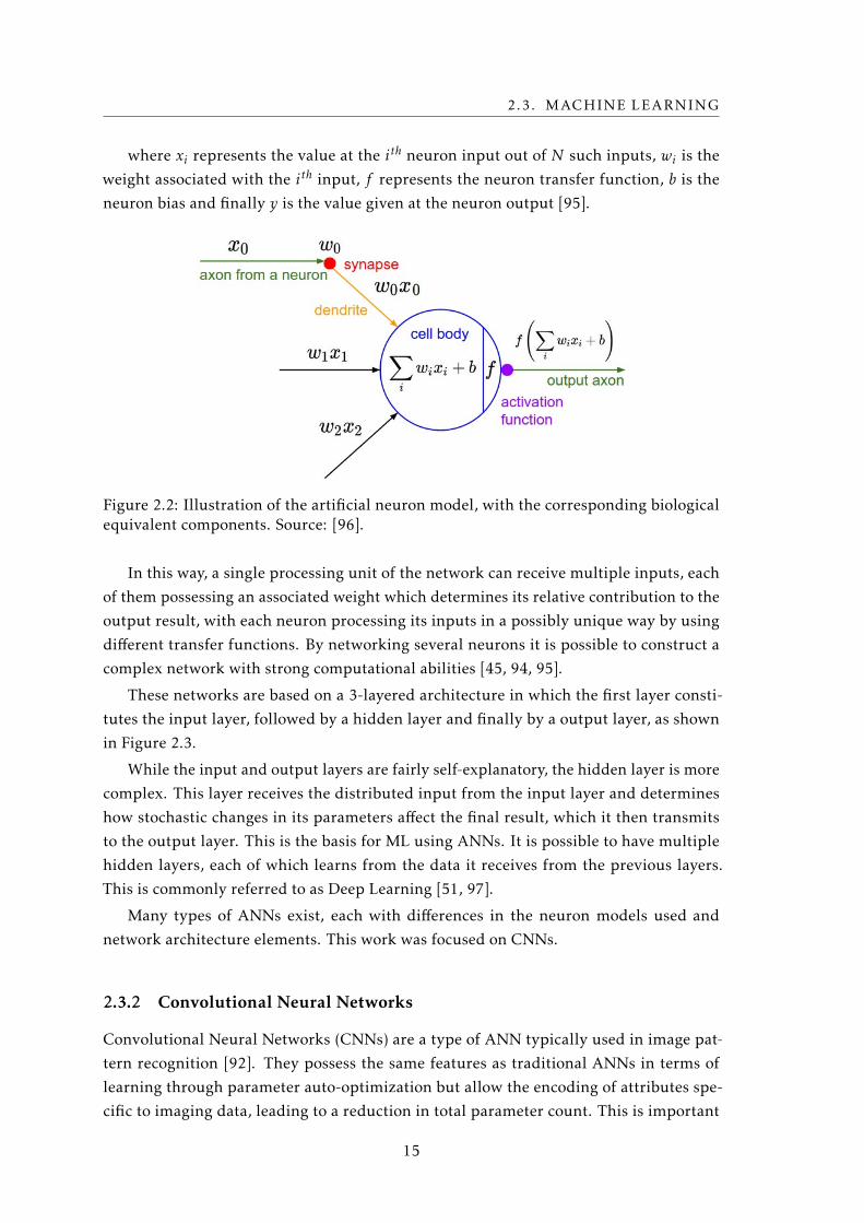
2.3. MACHINE LEARNING
where xi represents the value at the ith neuron input out of N such inputs, wi is the
weight associated with the ith input, f represents the neuron transfer function, b is the
neuron bias and finally y is the value given at the neuron output [95].
Figure 2.2: Illustration of the artificial neuron model, with the corresponding biologicalequivalent components. Source: [96].
In this way, a single processing unit of the network can receive multiple inputs, each
of them possessing an associated weight which determines its relative contribution to the
output result, with each neuron processing its inputs in a possibly unique way by using
different transfer functions. By networking several neurons it is possible to construct a
complex network with strong computational abilities [45, 94, 95].
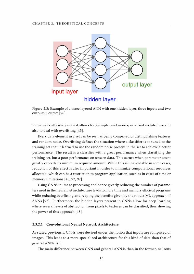
These networks are based on a 3-layered architecture in which the first layer consti-
tutes the input layer, followed by a hidden layer and finally by a output layer, as shown
in Figure 2.3.
While the input and output layers are fairly self-explanatory, the hidden layer is more
complex. This layer receives the distributed input from the input layer and determines
how stochastic changes in its parameters affect the final result, which it then transmits
to the output layer. This is the basis for ML using ANNs. It is possible to have multiple
hidden layers, each of which learns from the data it receives from the previous layers.
This is commonly referred to as Deep Learning [51, 97].
Many types of ANNs exist, each with differences in the neuron models used and
network architecture elements. This work was focused on CNNs.
2.3.2 Convolutional Neural Networks
Convolutional Neural Networks (CNNs) are a type of ANN typically used in image pat-
tern recognition [92]. They possess the same features as traditional ANNs in terms of
learning through parameter auto-optimization but allow the encoding of attributes spe-
cific to imaging data, leading to a reduction in total parameter count. This is important
15
CHAPTER 2. THEORETICAL CONCEPTS
Figure 2.3: Example of a three layered ANN with one hidden layer, three inputs and twooutputs. Source: [96].
for network efficiency since it allows for a simpler and more specialized architecture and
also to deal with overfitting [45].
Every data element in a set can be seen as being comprised of distinguishing features
and random noise. Overfitting defines the situation where a classifier is so tuned to the
training set that it learned to use the random noise present in the set to achieve a better
performance. The result is a classifier with a great performance when classifying the
training set, but a poor performance on unseen data. This occurs when parameter count
greatly exceeds its minimum required amount. While this is unavoidable in some cases,
reduction of this effect is also important in order to minimize computational resources
allocated, which can be a restriction to program application, such as in cases of time or
memory limitations [45, 92, 97].
Using CNNs in image processing and hence greatly reducing the number of parame-
ters used in the neural net architecture leads to more time and memory efficient programs
while reducing overfitting and reaping the benefits given by the robust ML approach of
ANNs [97]. Furthermore, the hidden layers present in CNNs allow for deep learning
where several levels of abstraction from pixels to textures can be classified, thus showing
the power of this approach [48].
2.3.2.1 Convolutional Neural Network Architecture
As stated previously, CNNs were devised under the notion that inputs are comprised of
images. This leads to a more specialized architecture for this kind of data than that of
general ANNs [45].
The main difference between CNN and general ANN is that, in the former, neurons
16
2.3. MACHINE LEARNING
comprising each layer are separated into 3 different sets, each representing a dimension
of the input: height, width and depth [45]. In this sense, three basic concepts are used in
the CNN algorithm [97]:
• Local Receptive Fields
• Parameter Sharing
• Pooling
These concepts are realized in the special layers which compose the CNN architecture,
which will be discussed in detail:
• Convolutional Layers
• Pooling Layers
• Fully-Connected Layers
Convolutional Layers are the most important layers in the CNN architecture and are
in fact the core building block of these networks. They rely on the use of learnable filters,
or kernels. In the Convolutional Layer, dot products are calculated between the filter and
small regions of the input at different locations of the image. The filter is dragged across
the image, producing a 2-dimensional activation map showing the responses of the filter
at each location of the input image [45, 96].
The aforementioned principle of Parameter Sharing can be seen here, as each filter
does not change depending on the location it is used in the image, and thereby reducing
parameter count and ensuring that a certain feature is found in different locations in
the image. Furthermore, the fact that each neuron is connected only to a limited section
of the previous layer, given by each location the filter is applied at, is denoted as the
neuron’s Local Receptive Field. This concept also allows for an enormous decrease in
overall parameter count and model complexity [45, 96].
As these filters are learnable (i.e. their values are adjusted to improve classifier per-
formance), it can be seen that certain distinguishing features of the image will produce
stronger responses for each filter and non-distinguishing features will generate weaker
responses. It is important to note that, while the first Convolutional layer can be easy to
comprehend as it allows to determine simple changes in pixel intensity (e.g. sharp colour
changes), Convolutional layers that lie further forward in the CNN architecture operate
on the output of the previous layers, i.e. on these activation maps (therefore denoted
as the layer’s input volume). This allows the network to distinguish more complex and
widespread patterns in the input image, therefore making a CNN able to distinguish
simple and complicated features in an image [45, 96].
An important matter to bear in mind is the optimisation of this layer in regards to
processing images. By applying the filters only on certain locations of the input volume,
17
CHAPTER 2. THEORETICAL CONCEPTS
the number of parameters required to define the network are greatly reduced, as opposed
to regular ANNs, where the input volume is fully connected to the layer input. This
allows for a smaller parameter count, thus reducing computational requirements and the
effects of overfitting [45].
A convolutional layer is defined by a set of parameters [45, 96]:
• Filter size - this corresponds to the dimension of the filters used in this layer.
Though these filters can have any 2-dimensional size, dimensions such as 3x3, 5x5
or up to 11x11 are typically used.
• Depth of the output volume - this corresponds to the number of filters that are
used in the layer, each searching for different features in the input volume.
• Stride - this denotes the amount of pixel shift between 2 consecutive filter applica-
tions.
• Zero-padding - this corresponds to the amount of zero-padding added to the bor-
ders of the input volume.
Pooling Layers are another important layer type in CNN architecture, applying the
aforementioned Pooling concept. A Pooling layer performs downsampling of its input vol-
ume along the spatial dimensionality. This greatly reduces model complexity and overall
parameter count, making Pooling Layers extremely important in any CNN architecture
[45, 96].
The pooling layer operates in a similar manner as the convolutional layer in the sense
that it also uses a filter which operates in certain locations of the image, locations which
are dictated by equivalent stride and filter size hyperparameters. Hence, this layer also
exhibits the concept of Local Receptive Field. However these filters are not learnable and
while in the convolutional layer a dot product is calculated at each location for several
filters, in the pooling layer a downsampling function is performed for a single filter. The
most common downsampling function is the max function, where the highest pixel value
among those encompassed by the filter is selected, though averaging the pixel values is
also another used approach (though much less common) [45, 96].
In terms of the size of the filter, very small filters (2x2 or 3x3) are usually preferred
due to the destructive nature of the pooling layer, though larger filter sizes may be used
[96].
Fully-Connected Layers are layers analogous to traditional ANNs where neurons
have full connections to all activations from the previous layer. The activation volume
resulting from a fully-connected layer can therefore be calculated by a simple matrix
multiplication with a bias offset. As such, in order to define a Fully-Connected Layer,
only the number of neurons in the layer is required [45, 96].
It is interesting to note that neurons in both Convolutional and Fully-Connected layers
perform a dot product with its inputs, the only difference between these layers being that
18
2.3. MACHINE LEARNING
the former has connections only to certain regions of its input volume, therefore justifying
the name of the Fully-Connected Layer [96].
Rectified Linear Unit (ReLU) Layers, though sometimes not listed as CNN layers
but rather as an optional operation of other layers, perform an elementwise activation
function, the most common of which is thresholding at zero, as seen in Equation (2.4)
[96]:
y =max(0,x) (2.4)
where x is the input, y the output and max defines the function which outputs the largest
of its input parameters.
In this work, ReLU operations are considered to be isolated layers since not doing so
would lead to a degree of ambiguity regarding the point in the architecture at which the
operation is performed (either before or after the associated layer). Considering it a layer
eliminates this ambiguity.
Unlike the other layers presented, this layer does not present any adjustable parame-
ters, but is used since it has proven to be a simple way to greatly increase training speed
and effectiveness without being too demanding in terms of computational resources [96].
After all the different layers which will process data, it becomes necessary to have a
manner in which the result of final layer is attributed to a class, i.e. the result is classified.
As such, a Score Function is used. Though not considered a layer, this is an indispensable
part of the network architecture [96].
The network’s score function denotes the operation that computes the class scores for
each prediction and is the final sequential element in a network. The 2 most commonly
used are the Support Vector Machine and the Softmax functions [96]. This work will
focus on the latter.
The Softmax function is a multiple class generalization of the binary Logistic Regres-
sion classifier. It is used to calculate a normalized probability score that the input belongs
to a certain class. Equation (2.5) describes this function [96]:
P (i) =exi
K∑j=1exj
(2.5)
where K denotes the number of data classes, x is a K-dimensional vector containing
the output of the last network layer and P (i) represents the normalized probability that
the function input is classified as the class of index i. By expanding to all i = 1, ...,K
the probability distribution of for all classes is obtained, with the sum of all its indices
equalling one.
19
CHAPTER 2. THEORETICAL CONCEPTS
2.3.2.2 Network Training
In order to train a CNN classifier, a few issues must be discussed to ensure training is
effective.
In every training round, it is necessary to gauge how well the model performs so that
it can adjust itself to improve performance. The algorithm used to perform this task is
called a Cost Function, or Loss Function. Many mathematical operations can be used to
this effect, but in this work we will focus on the Categorical Cross-entropy Cost Function,
which is a counterpart to the Softmax score function. It is computed using Equation (2.6),
with Equation (2.7) being used to compute the total cost [96]:
Li = − log
exyiK∑j=1exj
(2.6)
L =1N
N∑i=1
Li (2.7)
where yi represents the true class of input image i and so the argument of the loga-
rithm is the Softmax function, as presented in Equation (2.5), outputting the probability
score obtained for the true class of image i. As such, Li represents the cost (or data loss)
associated to input image i, with L representing the average loss across all N training
set images. This value is representative of network performance, where more efficient
networks have a lower associated L. The training process is guided toward the purpose
of lowering this value, thus improving network performance [96].
In obtaining the model cost value, a technique must be employed to evaluate the
degree of improvements that must be made to the network. Gradient Descent is a tech-
nique that consists in computing the gradient of the Cost Function for each parameter
throughout the training process. This way, it is possible to gauge how each parameter is
affecting performance so that they can be adjusted accordingly, i.e. backpropagated [96].
Many variations of this technique exist but in this work Root Mean Square Propagation
(RMSProp) will be used, which is a very effective adaptive learning rate method [98]
where a moving average of the squared gradient is kept for each parameter. This process
is described by Equation (2.8) and Equation (2.9) [99]:
E[g2]t = γ ×E[g2]t−1 + (1−γ)× g2t (2.8)
wt+1 = wt − gtη√
E[g2]t + ε(2.9)
where g denotes the gradient of the Cost Function and t denotes the training round
index, such that E[g2]t denotes the moving average of the squared gradient at training
round t. At each round, this moving average is updated according to Equation (2.8) so
that network parameters w can be updated according to Equation (2.9). Furthermore, γ
20
2.3. MACHINE LEARNING
defines the momentum term responsible for reducing oscillations in parameter optimiza-
tion and is usually set to 0.9, ε is the term responsible for decaying the moving average
value in parameter update and is usually set to 1× 10⁻⁶. Finally, the constant η, named
Learning Rate, is of particular interest as it dictates how strongly the gradient will affect
the parameter update, hence the name. In this case, it is suggested to be set to 0.001 [99].
The next issue that must be approached is the use of Regularization techniques. These
techniques focus on controlling the weight values so as to prevent the model from over-
fitting the data during training. There are several Regularization techniques which find
an application in CNN [96]:
• L2 regularization, or weight decay.
• L1 regularization
• Max norm constraints
• Dropout
In this work, the Dropout technique is used, as it is a very simple yet effective tech-
nique.
The Dropout technique consists in only keeping a neuron active with a certain prob-
ability p, and keeping it inactive otherwise. This process of activating/deactivating neu-
rons is repeated for each training round and for every neuron in the network [96].
Using Dropout, the network being trained will consist in a different configuration
in every training round (though maintaining its general architecture) and the weights
of each active neuron will adapt to their current configuration. While this may seem
counter intuitive, it can be compared to creating several similar networks and averaging
their classification results, which in itself is an effective technique to prevent a model
from overfitting. The difference, however, lays in the fact that a single network is being
trained, making this technique less computationally demanding [96].
The final issue is that of Weight Initialization. Before the first training round of
the network, weight values must have a starting value, which will then be adjusted as
the network is trained. These values must be sensibly initialized, as they determine the
point from which the network will progress through learning. If this starting point is not
appropriate, then the network may never perform well [96].
While initializing the weights to zero may seem like a simple solution that allows the
weights to be adjusted to both positive and negative values easily without compromising
the starting performance, it is actually a logical pitfall which compromises network per-
formance. This is due to the fact that every neuron will have the same starting conditions
and, as such, will be adjusted in the same way as training progresses, always comput-
ing the same output between themselves. As such, an appropriate weight initialization
scheme must introduce an element of asymmetry between the neurons [96].
21
CHAPTER 2. THEORETICAL CONCEPTS
A more appropriate way to initialize the weights is to assign them small random
values. This method is called symmetry-breaking and allows the neurons to evolve in-
dependently throughout training as unique components of a complex network, and the
small magnitude of the values avoids compromising the starting state of the network.
Initializing the weights in this way also avoids the need to define an initialization scheme
for the bias values, as asymmetries are already avoided by the random weights, allowing
the bias to also evolve independently of each other [96].
2.4 Cloud Computing
2.4.1 Definition
According to the National Institute of Standards and Technology (NIST) [100]:
Cloud Computing is a model for enabling ubiquitous, convenient, on-demandnetwork access to a shared pool of configurable computing resources (e.g., networks,servers, storage, applications, and services) that can be rapidly provisioned andreleased with minimal management effort or service provider interaction.
Essentially, Cloud Computing denotes a kind of on-demand Internet-based computing
where users interact with the underlying Cloud infrastructure in 5 different deployment
models and 3 different service models [65, 66, 101], which will be discussed shortly.
The underlying Cloud infrastructure is composed of autonomous networked physical
and abstract components. The physical components denote the hardware and the abstract
ones denote the software which are the basis for the essential Cloud features presented
above [65, 66, 101].
NIST also specifies 5 essential characteristics for the Cloud model [100]:
1. The user can independently access the cloud resources without the need for human
interaction.
2. Cloud resources and services are available through standard network-accessing
mechanisms.
3. The Cloud resources are pooled to serve multiple users simultaneously, with re-
sources being dynamically assigned according to the needs of each user.
4. The Cloud capabilities are scalable and can be elastically expanded or contracted
according to user and system needs.
5. Resource use is optimized by the Cloud and its use is transparent.
22
2.4. CLOUD COMPUTING
2.4.2 Deployment Models
NIST recognizes four different methodologies in which Access privileges to a Cloud en-
vironment can be granted, and as such four different Cloud Deployment Models can be
distinguished [100]:
• Public Cloud - The Cloud is accessible to the general public.
• Private Cloud - Cloud access is restricted to consumers or members of consumer
organizations.
• Hybrid Cloud - Cloud infrastructure is composed of multiple distinct Cloud in-
frastructures with varying deployment models. These infrastructures are bound
together to allow inter-Cloud operations.
• Community Cloud - Cloud access is shared between members of a community with
similar concerns of whatever kind. This model stands between that of the PublicPrivate clouds, as the access is not fully open but neither is it private.
2.4.3 Cloud Service Models
In the Cloud Computing model, there are three generally recognizable ways in which a
Cloud provider offers their service. These differing approaches are denoted as Service
Models [100]:
2.4.3.1 Software-as-a-Service (SaaS)
In this model, the user is given access to software placed on the cloud by the provider. This
way, the user can remotely access capabilities which he does not own and the provider
can enable that access without any product delivery. This is the more standard definition
of a Cloud service and the more commonly employed. The user is given access only to
the software and cannot control the underlying infrastructure, as the software should
be self-sufficient in the sense that it can manage Cloud resources to ensure its correct
function. SaaS is, therefore, browser interface software through a network to a Cloud [65,
66].
2.4.3.2 Platform-as-a-Service (PaaS)
In this model, the user is given remote computational capabilities to implement or cre-
ate software that can be implemented and run on the Cloud, but is not given access to
the underlying infrastructure, save being able to manage functionalities regarding the
deployment of the applications. This model usually entails providing a set of libraries
and Cloud programming functionalities to enable the creation of user applications to be
implemented on the Cloud [65, 66].
23

CHAPTER 2. THEORETICAL CONCEPTS
2.4.3.3 Infrastructure-as-a-Service (IaaS)
In this model, the user is provided with the computational capabilities of Cloud hardware,
being able to fully manage the Cloud resources to set up programs and change system
specifications. The user cannot, however, access core Cloud functionalities. The purpose
of this model is to provide remote access to computational hardware without the need to
own it, but with all the customisation ability of possessing ownership [65, 66].
24
Chapter
3Materials & Methods
3.1 Application
In order to develop a classifier, a ML framework which included CNN algorithms had to
be chosen. The chosen framework was Theano©.
3.1.1 Theano© framework
Theano© is an open-source Python library used for the purpose of efficiently defining,
optimizing and evaluating mathematical expressions involving multi-dimensional arrays.
It was created in 2008 and since then has seen continuous development and multiple
other frameworks have been built on top of it, including several State-of-the-Art ML
models [102].
Theano was designed to function both with a Central Processing Unit (CPU) or a
Graphics Processing Unit (GPU) and to facilitate the shift between them. Furthermore,
the advantage of using Theano lies in its optimization techniques, as it avoids redundan-
cies in computations, simplifies mathematical expressions, continuously tries to minimize
both memory use and errors that arise from hardware approximations [102].
Theano uses the Python programming language as an interface, taking advantage of
its widespread use in the scientific community. The popularity of this language comes
from the fact that it is both open source and was designed to be easily legible and compre-
hensible. This lead to numerous different libraries being built on top of Python, namely
NumPy and SciPy, which came to wide use in the scientific community. The use of this
language and the fact that Theano’s programming interface closely resembles NumPy, a
popular mathematical Python library, promotes its usability and has contributed to its
acceptance in the context of ML development [102, 103].
25
CHAPTER 3. MATERIALS & METHODS
The fact that Theano is completely accessible through the Python language provides
an advantage in the sense that, as long as Theano is correctly configured, one needs only
to focus on developing the application front-end in Python and thus more easily separate
the computational aspect of the application from the user interface. Furthermore, while
Theano is widely used in the ML context, it is not solely a ML application, but rather a
mathematical optimization one. This increases the advantages of using Theano in the
sense that the application will be easily expandable and new features not necessarily
involved in direct CNN development can be implemented [102].
To note that another ML framework was used: Caffe©, which is specialized in CNN
classification [104]. One feature that was developed, as will be discussed in a later chapter,
was a compatibility between this framework and the application. It was in this context
that Caffe was used, and hence the application does not employ it for network training
or classification of data.
3.1.2 Microsoft Azure®
Microsoft Azure® is a collection of integrated cloud computing services which can be
used to create, implement and manage applications resorting to the Cloud paradigm. It
provides all deployment models referenced in Section 2.4.3 and supports several pro-
gramming languages, tools and frameworks [105].
Due to the inherent intricacies involved in the installation of Theano, namely the
need to make changes in the file system, an IaaS approach was taken by making use
of the Azure Virtual Machine functionality, where a Cloud-based virtual machine is
used. Though following an IaaS approach, these environments come with a pre-installed
Operating System. To create the virtual machine the user needs to select the desired
computational capabilities of the environment, including pricing details.
Bearing in mind the license used, the chosen virtual machine featured a Linux Operat-
ing System with a 4-core CPU, 14 gigabytes of memory and local Solid-State Drive (SSD)
storage of 28 gigabytes. While virtual machines with more processing capabilities were
available, including access to GPUs, the available license limited the ability to choose one
such machine, and as such the most affordable virtual machine was chosen.
3.1.3 Flask© Microframework
While the classifier computations are handled by Theano, a user interface is required in
order to provide a means for users to interact with the application. For this purpose, the
Flask microframework was used.
Flask© is a web development microframework for Python based on Werkzeug© and
Jinja2©. It is usually referred to as a microframework due to its relative simplicity while
still maintaining extensibility and functionality. It allows the user to create websites
using the Python language and thus interface with any Python code [106].
26
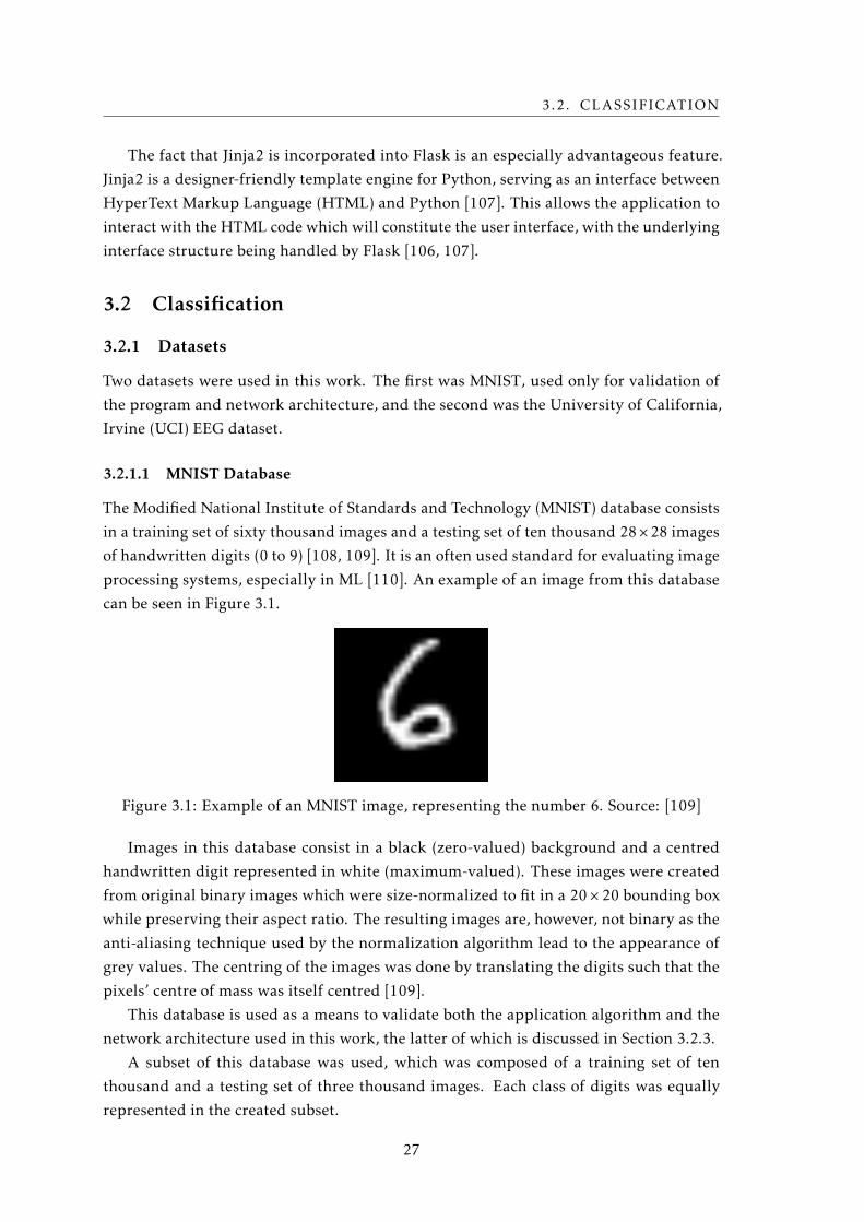
3.2. CLASSIFICATION
The fact that Jinja2 is incorporated into Flask is an especially advantageous feature.
Jinja2 is a designer-friendly template engine for Python, serving as an interface between
HyperText Markup Language (HTML) and Python [107]. This allows the application to
interact with the HTML code which will constitute the user interface, with the underlying
interface structure being handled by Flask [106, 107].
3.2 Classification
3.2.1 Datasets
Two datasets were used in this work. The first was MNIST, used only for validation of
the program and network architecture, and the second was the University of California,
Irvine (UCI) EEG dataset.
3.2.1.1 MNIST Database
The Modified National Institute of Standards and Technology (MNIST) database consists
in a training set of sixty thousand images and a testing set of ten thousand 28×28 images
of handwritten digits (0 to 9) [108, 109]. It is an often used standard for evaluating image
processing systems, especially in ML [110]. An example of an image from this database
can be seen in Figure 3.1.
Figure 3.1: Example of an MNIST image, representing the number 6. Source: [109]
Images in this database consist in a black (zero-valued) background and a centred
handwritten digit represented in white (maximum-valued). These images were created
from original binary images which were size-normalized to fit in a 20× 20 bounding box
while preserving their aspect ratio. The resulting images are, however, not binary as the
anti-aliasing technique used by the normalization algorithm lead to the appearance of
grey values. The centring of the images was done by translating the digits such that the
pixels’ centre of mass was itself centred [109].
This database is used as a means to validate both the application algorithm and the
network architecture used in this work, the latter of which is discussed in Section 3.2.3.
A subset of this database was used, which was composed of a training set of ten
thousand and a testing set of three thousand images. Each class of digits was equally
represented in the created subset.
27
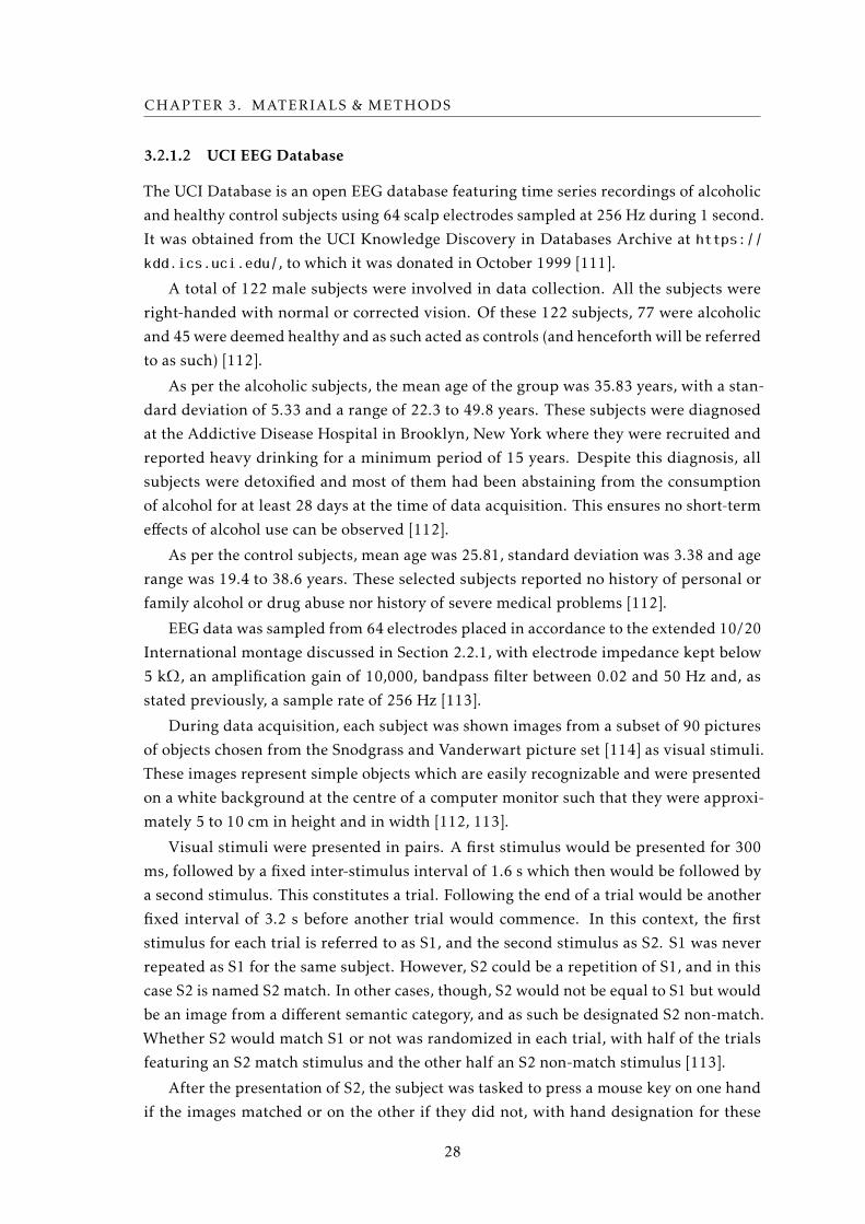
CHAPTER 3. MATERIALS & METHODS
3.2.1.2 UCI EEG Database
The UCI Database is an open EEG database featuring time series recordings of alcoholic
and healthy control subjects using 64 scalp electrodes sampled at 256 Hz during 1 second.
It was obtained from the UCI Knowledge Discovery in Databases Archive at https://
kdd.ics.uci.edu/, to which it was donated in October 1999 [111].
A total of 122 male subjects were involved in data collection. All the subjects were
right-handed with normal or corrected vision. Of these 122 subjects, 77 were alcoholic
and 45 were deemed healthy and as such acted as controls (and henceforth will be referred
to as such) [112].
As per the alcoholic subjects, the mean age of the group was 35.83 years, with a stan-
dard deviation of 5.33 and a range of 22.3 to 49.8 years. These subjects were diagnosed
at the Addictive Disease Hospital in Brooklyn, New York where they were recruited and
reported heavy drinking for a minimum period of 15 years. Despite this diagnosis, all
subjects were detoxified and most of them had been abstaining from the consumption
of alcohol for at least 28 days at the time of data acquisition. This ensures no short-term
effects of alcohol use can be observed [112].
As per the control subjects, mean age was 25.81, standard deviation was 3.38 and age
range was 19.4 to 38.6 years. These selected subjects reported no history of personal or
family alcohol or drug abuse nor history of severe medical problems [112].
EEG data was sampled from 64 electrodes placed in accordance to the extended 10/20
International montage discussed in Section 2.2.1, with electrode impedance kept below
5 kΩ, an amplification gain of 10,000, bandpass filter between 0.02 and 50 Hz and, as
stated previously, a sample rate of 256 Hz [113].
During data acquisition, each subject was shown images from a subset of 90 pictures
of objects chosen from the Snodgrass and Vanderwart picture set [114] as visual stimuli.
These images represent simple objects which are easily recognizable and were presented
on a white background at the centre of a computer monitor such that they were approxi-
mately 5 to 10 cm in height and in width [112, 113].
Visual stimuli were presented in pairs. A first stimulus would be presented for 300
ms, followed by a fixed inter-stimulus interval of 1.6 s which then would be followed by
a second stimulus. This constitutes a trial. Following the end of a trial would be another
fixed interval of 3.2 s before another trial would commence. In this context, the first
stimulus for each trial is referred to as S1, and the second stimulus as S2. S1 was never
repeated as S1 for the same subject. However, S2 could be a repetition of S1, and in this
case S2 is named S2 match. In other cases, though, S2 would not be equal to S1 but would
be an image from a different semantic category, and as such be designated S2 non-match.
Whether S2 would match S1 or not was randomized in each trial, with half of the trials
featuring an S2 match stimulus and the other half an S2 non-match stimulus [113].
After the presentation of S2, the subject was tasked to press a mouse key on one hand
if the images matched or on the other if they did not, with hand designation for these
28
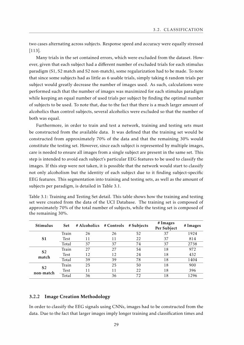
3.2. CLASSIFICATION
two cases alternating across subjects. Response speed and accuracy were equally stressed
[113].
Many trials in the set contained errors, which were excluded from the dataset. How-
ever, given that each subject had a different number of excluded trials for each stimulus
paradigm (S1, S2 match and S2 non-match), some regularization had to be made. To note
that since some subjects had as little as 6 usable trials, simply taking 6 random trials per
subject would greatly decrease the number of images used. As such, calculations were
performed such that the number of images was maximized for each stimulus paradigm
while keeping an equal number of used trials per subject by finding the optimal number
of subjects to be used. To note that, due to the fact that there is a much larger amount of
alcoholics than control subjects, several alcoholics were excluded so that the number of
both was equal.
Furthermore, in order to train and test a network, training and testing sets must
be constructed from the available data. It was defined that the training set would be
constructed from approximately 70% of the data and that the remaining 30% would
constitute the testing set. However, since each subject is represented by multiple images,
care is needed to ensure all images from a single subject are present in the same set. This
step is intended to avoid each subject’s particular EEG features to be used to classify the
images. If this step were not taken, it is possible that the network would start to classify
not only alcoholism but the identity of each subject due to it finding subject-specific
EEG features. This segmentation into training and testing sets, as well as the amount of
subjects per paradigm, is detailed in Table 3.1.
Table 3.1: Training and Testing Set detail. This table shows how the training and testingset were created from the data of the UCI Database. The training set is composed ofapproximately 70% of the total number of subjects, while the testing set is composed ofthe remaining 30%.
Stimulus Set # Alcoholics # Controls # Subjects# Images
Per Subject# Images
S1Train 26 26 52 37 1924Test 11 11 22 37 814Total 37 37 74 37 2738
S2match
Train 27 27 54 18 972Test 12 12 24 18 432Total 39 39 78 18 1404
S2non-match
Train 25 25 50 18 900Test 11 11 22 18 396Total 36 36 72 18 1296
3.2.2 Image Creation Methodology
In order to classify the EEG signals using CNNs, images had to be constructed from the
data. Due to the fact that larger images imply longer training and classification times and
29
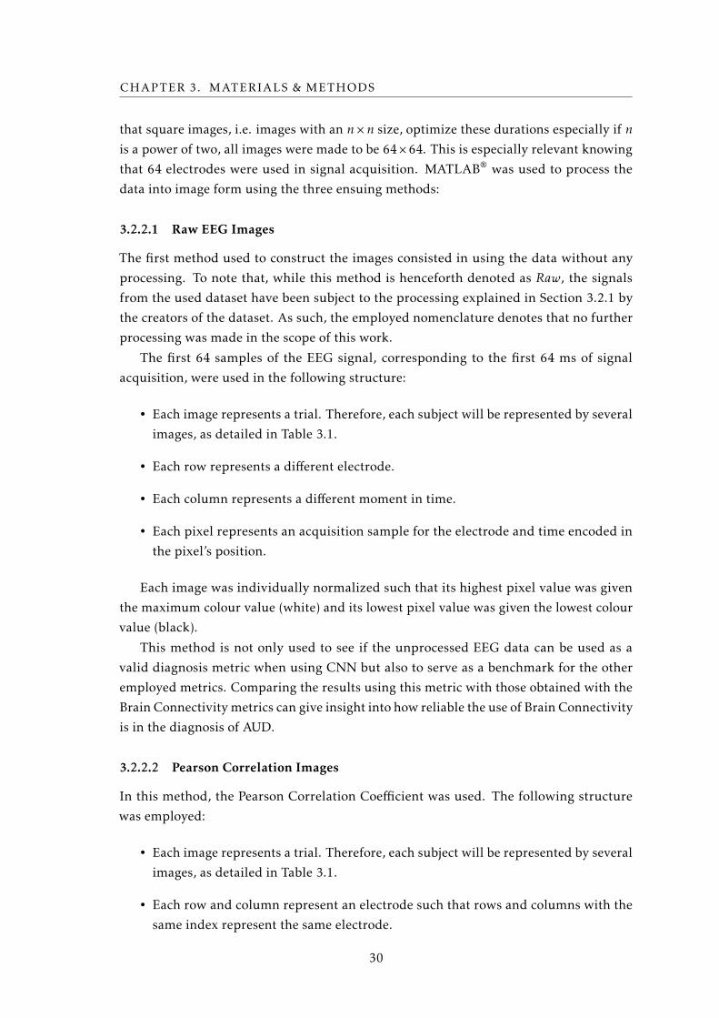
CHAPTER 3. MATERIALS & METHODS
that square images, i.e. images with an n×n size, optimize these durations especially if n
is a power of two, all images were made to be 64×64. This is especially relevant knowing
that 64 electrodes were used in signal acquisition. MATLAB® was used to process the
data into image form using the three ensuing methods:
3.2.2.1 Raw EEG Images
The first method used to construct the images consisted in using the data without any
processing. To note that, while this method is henceforth denoted as Raw, the signals
from the used dataset have been subject to the processing explained in Section 3.2.1 by
the creators of the dataset. As such, the employed nomenclature denotes that no further
processing was made in the scope of this work.
The first 64 samples of the EEG signal, corresponding to the first 64 ms of signal
acquisition, were used in the following structure:
• Each image represents a trial. Therefore, each subject will be represented by several
images, as detailed in Table 3.1.
• Each row represents a different electrode.
• Each column represents a different moment in time.
• Each pixel represents an acquisition sample for the electrode and time encoded in
the pixel’s position.
Each image was individually normalized such that its highest pixel value was given
the maximum colour value (white) and its lowest pixel value was given the lowest colour
value (black).
This method is not only used to see if the unprocessed EEG data can be used as a
valid diagnosis metric when using CNN but also to serve as a benchmark for the other
employed metrics. Comparing the results using this metric with those obtained with the
Brain Connectivity metrics can give insight into how reliable the use of Brain Connectivity
is in the diagnosis of AUD.
3.2.2.2 Pearson Correlation Images
In this method, the Pearson Correlation Coefficient was used. The following structure
was employed:
• Each image represents a trial. Therefore, each subject will be represented by several
images, as detailed in Table 3.1.
• Each row and column represent an electrode such that rows and columns with the
same index represent the same electrode.
30

3.2. CLASSIFICATION
• Each pixel represents the Pearson Correlation Coefficient between the signals given
by the electrodes encoded in the pixel’s position.
The constructed images were normalized so that the lowest possible value obtain-
able from the Pearson Correlation Coefficient calculation, −1, represented black and the
highest obtainable value, +1, represented white.
3.2.2.3 Maximum Cross-Correlation Images
In this case, the maximum value of the normalized Cross-Correlation spectrum between
the signals of two electrodes was used as a metric. Usage of this method was based on its
use by Mirowski et al. [59] and it is obtained with Equation (3.1):
MCCx,y = maxτ
∣∣∣∣∣∣∣∣∣
Cx,y(τ)√Cx,x(0) ·Cy,y(0)
∣∣∣∣∣∣∣∣∣ (3.1)
Similar to the interpretation of the Cross-Correlation in Section 2.2.2.2, this metric
indicates the strength of the linear relationship between two signals. This specific metric,
however, outputs the highest value of correlation between two signals for every lag. The
fact that the spectrum is normalized means the relative strength of the highest Cross-
Correlation value, in comparison with the rest of the spectrum, is obtained.
Therefore, if two electrodes possess a strong linear relationship at a certain delay
between them, the resultant value for this metric will be high. If, on the other hand,
the signals do not show a strong linear relationship for a certain lag between them, then
the spectrum will be flatter and, as such, the value obtained from this metric will be low.
Thus, this metric shows indication of whether a certain delay leads to a relatively stronger
linear relationship between the two signals.
The following data structure was employed:
• Each image represents a trial. Therefore, each subject will be represented by several
images, as detailed in Table 3.1.
• Each row and column represent an electrode such that rows and columns with the
same index represent the same electrode.
• Each pixel represents the Maximum Cross-Correlation between the signals given
by the electrodes encoded in the pixel’s position.
Due to the fact that the maximum value of the Cross-Correlation spectrum is being
used, values will always be positive. As such, each image was individually normalized
such that its highest pixel value was given the maximum colour value (white) and its
lowest pixel value was given the lowest colour value (black).
31
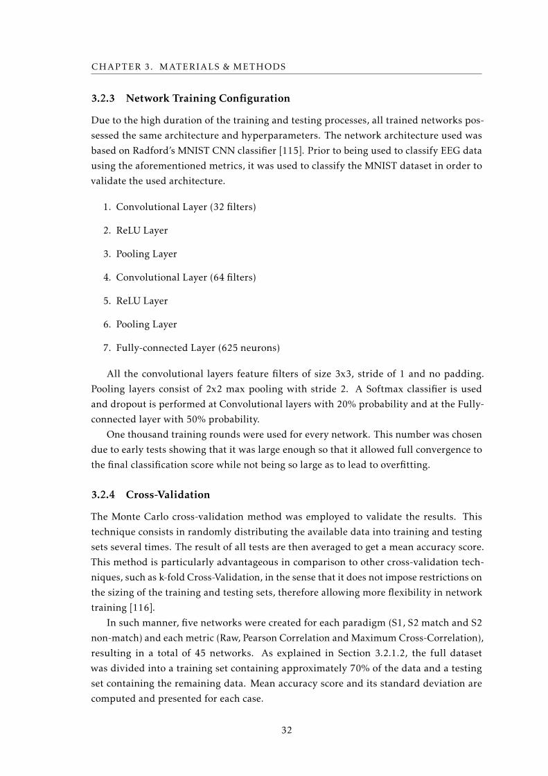
CHAPTER 3. MATERIALS & METHODS
3.2.3 Network Training Configuration
Due to the high duration of the training and testing processes, all trained networks pos-
sessed the same architecture and hyperparameters. The network architecture used was
based on Radford’s MNIST CNN classifier [115]. Prior to being used to classify EEG data
using the aforementioned metrics, it was used to classify the MNIST dataset in order to
validate the used architecture.
1. Convolutional Layer (32 filters)
2. ReLU Layer
3. Pooling Layer
4. Convolutional Layer (64 filters)
5. ReLU Layer
6. Pooling Layer
7. Fully-connected Layer (625 neurons)
All the convolutional layers feature filters of size 3x3, stride of 1 and no padding.
Pooling layers consist of 2x2 max pooling with stride 2. A Softmax classifier is used
and dropout is performed at Convolutional layers with 20% probability and at the Fully-
connected layer with 50% probability.
One thousand training rounds were used for every network. This number was chosen
due to early tests showing that it was large enough so that it allowed full convergence to
the final classification score while not being so large as to lead to overfitting.
3.2.4 Cross-Validation
The Monte Carlo cross-validation method was employed to validate the results. This
technique consists in randomly distributing the available data into training and testing
sets several times. The result of all tests are then averaged to get a mean accuracy score.
This method is particularly advantageous in comparison to other cross-validation tech-
niques, such as k-fold Cross-Validation, in the sense that it does not impose restrictions on
the sizing of the training and testing sets, therefore allowing more flexibility in network
training [116].
In such manner, five networks were created for each paradigm (S1, S2 match and S2
non-match) and each metric (Raw, Pearson Correlation and Maximum Cross-Correlation),
resulting in a total of 45 networks. As explained in Section 3.2.1.2, the full dataset
was divided into a training set containing approximately 70% of the data and a testing
set containing the remaining data. Mean accuracy score and its standard deviation are
computed and presented for each case.
32
Chapter
4Results & Discussion
4.1 Application
The application was created and housed, as intended, in an Azure Cloud server and
features two main functionalities: the ability to create and train Convolutional Neural
Networks and the ability to employ an existing one for classification. In order to be
accessible to users, a website is used as a front-end.
In this section, the created application will be explored in detail. First, the guiding
principles behind the interface will be discussed, followed by the main structure of the
front-end website. A more detailed scope of the structure will be shown as the main
functionalities (network creation/training and classification) are presented. Next, a set
of specific relevant features of the application will be analysed, namely the possibility to
create networks with a custom architecture, the ability to import Caffe networks and the
data labelling strategy employed. Finally, the matter of processing time and the use of a
Cloud environment will be evaluated.
Beyond presenting these features, their relevance and importance will also be dis-
cussed and analysed.
4.1.1 Interface
Since the underlying application code is complex, a simple interface is an important and
relevant feature to be discussed. Due to the fact that the application front-end consists of
a website, the use of HTML and Cascading Style Sheets (CSS) provides the ability to create
appealing and adaptable visual elements. Also, the use of Jinja2 allows extensive changes
to the visual aspect of the website to be very simple, requiring only the modification of a
single file to make changes to all sub-pages of the website.
33
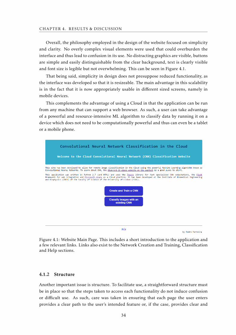
CHAPTER 4. RESULTS & DISCUSSION
Overall, the philosophy employed in the design of the website focused on simplicity
and clarity. No overly complex visual elements were used that could overburden the
interface and thus lead to confusion in its use. No distracting graphics are visible, buttons
are simple and easily distinguishable from the clear background, text is clearly visible
and font size is legible but not overwhelming. This can be seen in Figure 4.1.
That being said, simplicity in design does not presuppose reduced functionality, as
the interface was developed so that it is resizeable. The main advantage in this scalability
is in the fact that it is now appropriately usable in different sized screens, namely in
mobile devices.
This complements the advantage of using a Cloud in that the application can be run
from any machine that can support a web browser. As such, a user can take advantage
of a powerful and resource-intensive ML algorithm to classify data by running it on a
device which does not need to be computationally powerful and thus can even be a tablet
or a mobile phone.
Figure 4.1: Website Main Page. This includes a short introduction to the application anda few relevant links. Links also exist to the Network Creation and Training, Classificationand Help sections.
4.1.2 Structure
Another important issue is structure. To facilitate use, a straightforward structure must
be in place so that the steps taken to access each functionality do not induce confusion
or difficult use. As such, care was taken in ensuring that each page the user enters
provides a clear path to the user’s intended feature or, if the case, provides clear and
34
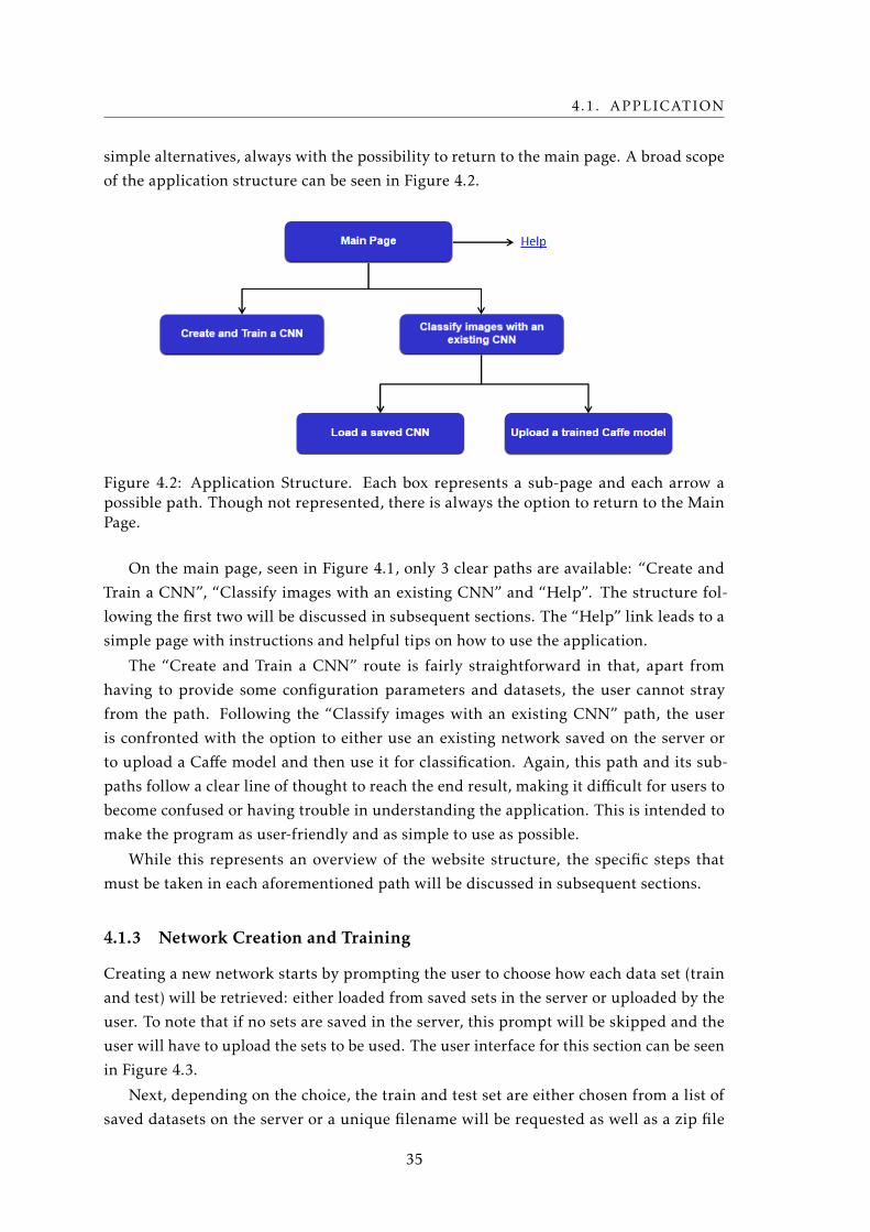
4.1. APPLICATION
simple alternatives, always with the possibility to return to the main page. A broad scope
of the application structure can be seen in Figure 4.2.
Figure 4.2: Application Structure. Each box represents a sub-page and each arrow apossible path. Though not represented, there is always the option to return to the MainPage.
On the main page, seen in Figure 4.1, only 3 clear paths are available: “Create and
Train a CNN”, “Classify images with an existing CNN” and “Help”. The structure fol-
lowing the first two will be discussed in subsequent sections. The “Help” link leads to a
simple page with instructions and helpful tips on how to use the application.
The “Create and Train a CNN” route is fairly straightforward in that, apart from
having to provide some configuration parameters and datasets, the user cannot stray
from the path. Following the “Classify images with an existing CNN” path, the user
is confronted with the option to either use an existing network saved on the server or
to upload a Caffe model and then use it for classification. Again, this path and its sub-
paths follow a clear line of thought to reach the end result, making it difficult for users to
become confused or having trouble in understanding the application. This is intended to
make the program as user-friendly and as simple to use as possible.
While this represents an overview of the website structure, the specific steps that
must be taken in each aforementioned path will be discussed in subsequent sections.
4.1.3 Network Creation and Training
Creating a new network starts by prompting the user to choose how each data set (train
and test) will be retrieved: either loaded from saved sets in the server or uploaded by the
user. To note that if no sets are saved in the server, this prompt will be skipped and the
user will have to upload the sets to be used. The user interface for this section can be seen
in Figure 4.3.
Next, depending on the choice, the train and test set are either chosen from a list of
saved datasets on the server or a unique filename will be requested as well as a zip file
35
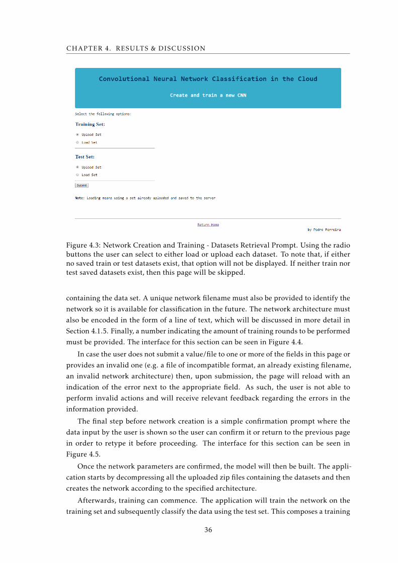
CHAPTER 4. RESULTS & DISCUSSION
Figure 4.3: Network Creation and Training - Datasets Retrieval Prompt. Using the radiobuttons the user can select to either load or upload each dataset. To note that, if eitherno saved train or test datasets exist, that option will not be displayed. If neither train nortest saved datasets exist, then this page will be skipped.
containing the data set. A unique network filename must also be provided to identify the
network so it is available for classification in the future. The network architecture must
also be encoded in the form of a line of text, which will be discussed in more detail in
Section 4.1.5. Finally, a number indicating the amount of training rounds to be performed
must be provided. The interface for this section can be seen in Figure 4.4.
In case the user does not submit a value/file to one or more of the fields in this page or
provides an invalid one (e.g. a file of incompatible format, an already existing filename,
an invalid network architecture) then, upon submission, the page will reload with an
indication of the error next to the appropriate field. As such, the user is not able to
perform invalid actions and will receive relevant feedback regarding the errors in the
information provided.
The final step before network creation is a simple confirmation prompt where the
data input by the user is shown so the user can confirm it or return to the previous page
in order to retype it before proceeding. The interface for this section can be seen in
Figure 4.5.
Once the network parameters are confirmed, the model will then be built. The appli-
cation starts by decompressing all the uploaded zip files containing the datasets and then
creates the network according to the specified architecture.
Afterwards, training can commence. The application will train the network on the
training set and subsequently classify the data using the test set. This composes a training
36
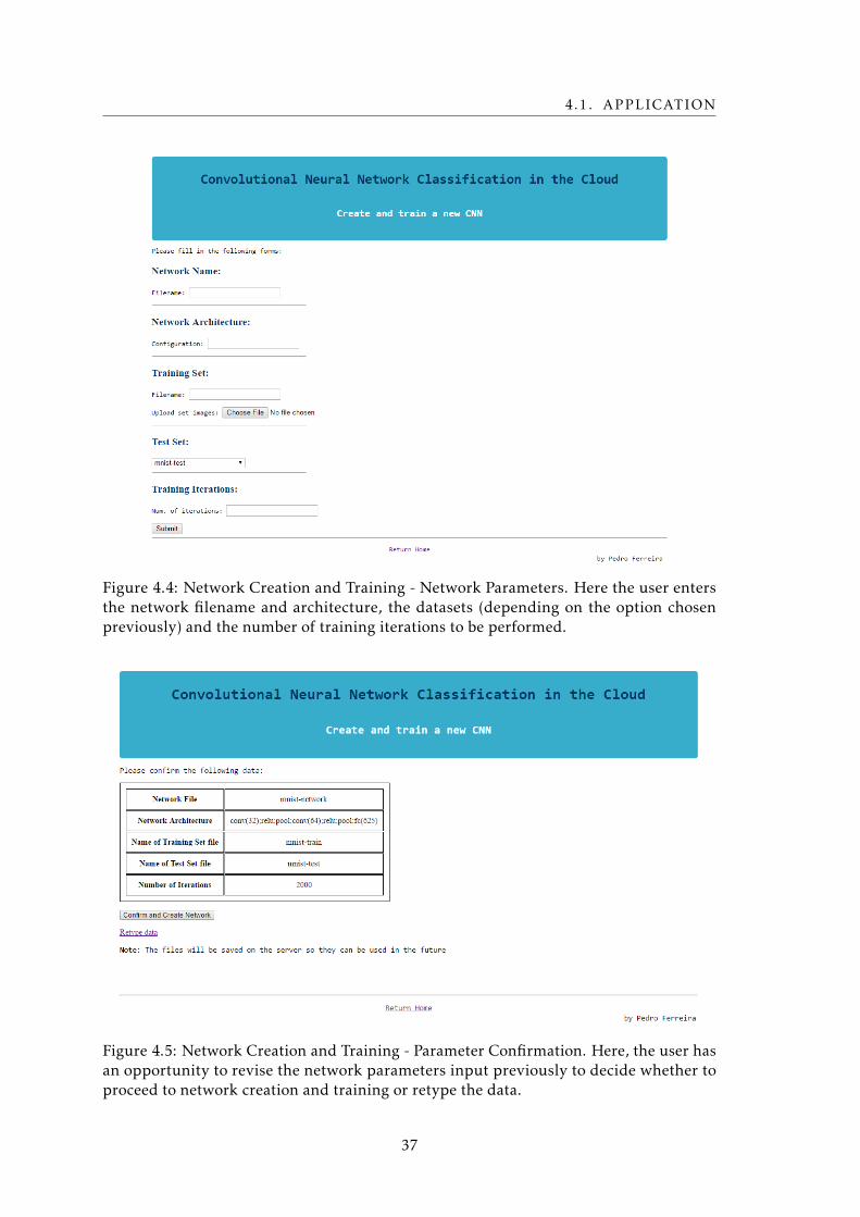
4.1. APPLICATION
Figure 4.4: Network Creation and Training - Network Parameters. Here the user entersthe network filename and architecture, the datasets (depending on the option chosenpreviously) and the number of training iterations to be performed.
Figure 4.5: Network Creation and Training - Parameter Confirmation. Here, the user hasan opportunity to revise the network parameters input previously to decide whether toproceed to network creation and training or retype the data.
37
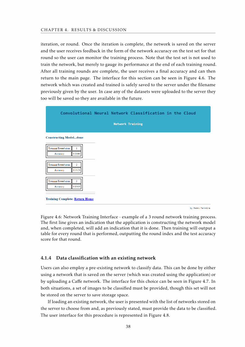
CHAPTER 4. RESULTS & DISCUSSION
iteration, or round. Once the iteration is complete, the network is saved on the server
and the user receives feedback in the form of the network accuracy on the test set for that
round so the user can monitor the training process. Note that the test set is not used to
train the network, but merely to gauge its performance at the end of each training round.
After all training rounds are complete, the user receives a final accuracy and can then
return to the main page. The interface for this section can be seen in Figure 4.6. The
network which was created and trained is safely saved to the server under the filename
previously given by the user. In case any of the datasets were uploaded to the server they
too will be saved so they are available in the future.
Figure 4.6: Network Training Interface - example of a 3 round network training process.The first line gives an indication that the application is constructing the network modeland, when completed, will add an indication that it is done. Then training will output atable for every round that is performed, outputting the round index and the test accuracyscore for that round.
4.1.4 Data classification with an existing network
Users can also employ a pre-existing network to classify data. This can be done by either
using a network that is saved on the server (which was created using the application) or
by uploading a Caffe network. The interface for this choice can be seen in Figure 4.7. In
both situations, a set of images to be classified must be provided, though this set will not
be stored on the server to save storage space.
If loading an existing network, the user is presented with the list of networks stored on
the server to choose from and, as previously stated, must provide the data to be classified.
The user interface for this procedure is represented in Figure 4.8.
38
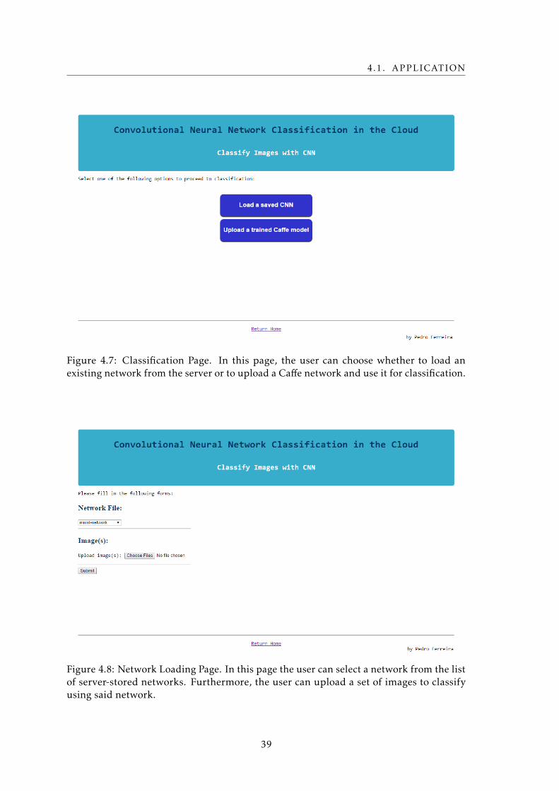
4.1. APPLICATION
Figure 4.7: Classification Page. In this page, the user can choose whether to load anexisting network from the server or to upload a Caffe network and use it for classification.
Figure 4.8: Network Loading Page. In this page the user can select a network from the listof server-stored networks. Furthermore, the user can upload a set of images to classifyusing said network.
39
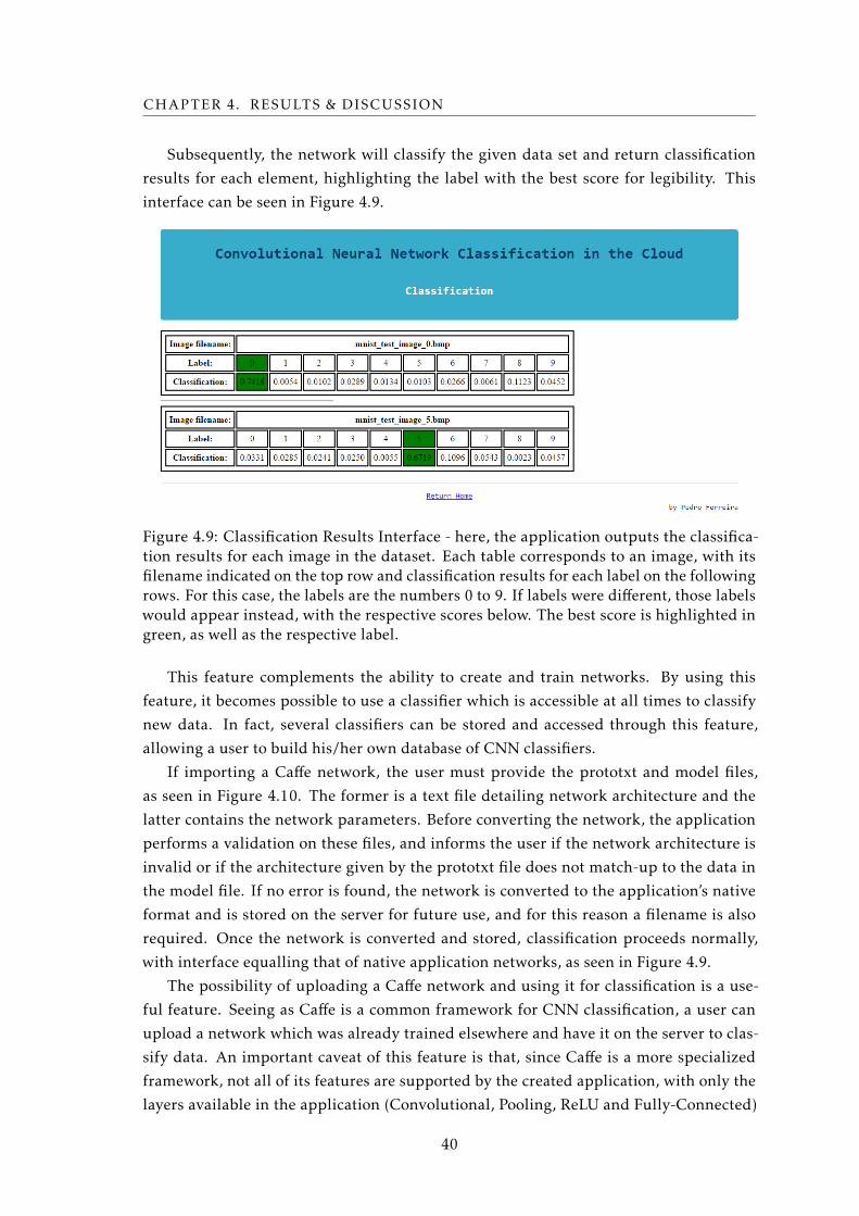
CHAPTER 4. RESULTS & DISCUSSION
Subsequently, the network will classify the given data set and return classification
results for each element, highlighting the label with the best score for legibility. This
interface can be seen in Figure 4.9.
Figure 4.9: Classification Results Interface - here, the application outputs the classifica-tion results for each image in the dataset. Each table corresponds to an image, with itsfilename indicated on the top row and classification results for each label on the followingrows. For this case, the labels are the numbers 0 to 9. If labels were different, those labelswould appear instead, with the respective scores below. The best score is highlighted ingreen, as well as the respective label.
This feature complements the ability to create and train networks. By using this
feature, it becomes possible to use a classifier which is accessible at all times to classify
new data. In fact, several classifiers can be stored and accessed through this feature,
allowing a user to build his/her own database of CNN classifiers.
If importing a Caffe network, the user must provide the prototxt and model files,
as seen in Figure 4.10. The former is a text file detailing network architecture and the
latter contains the network parameters. Before converting the network, the application
performs a validation on these files, and informs the user if the network architecture is
invalid or if the architecture given by the prototxt file does not match-up to the data in
the model file. If no error is found, the network is converted to the application’s native
format and is stored on the server for future use, and for this reason a filename is also
required. Once the network is converted and stored, classification proceeds normally,
with interface equalling that of native application networks, as seen in Figure 4.9.
The possibility of uploading a Caffe network and using it for classification is a use-
ful feature. Seeing as Caffe is a common framework for CNN classification, a user can
upload a network which was already trained elsewhere and have it on the server to clas-
sify data. An important caveat of this feature is that, since Caffe is a more specialized
framework, not all of its features are supported by the created application, with only the
layers available in the application (Convolutional, Pooling, ReLU and Fully-Connected)
40
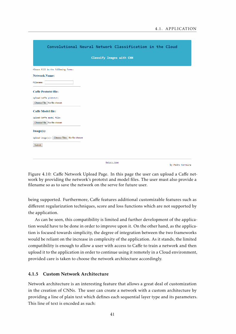
4.1. APPLICATION
Figure 4.10: Caffe Network Upload Page. In this page the user can upload a Caffe net-work by providing the network’s prototxt and model files. The user must also provide afilename so as to save the network on the serve for future user.
being supported. Furthermore, Caffe features additional customizable features such as
different regularization techniques, score and loss functions which are not supported by
the application.
As can be seen, this compatibility is limited and further development of the applica-
tion would have to be done in order to improve upon it. On the other hand, as the applica-
tion is focused towards simplicity, the degree of integration between the two frameworks
would be reliant on the increase in complexity of the application. As it stands, the limited
compatibility is enough to allow a user with access to Caffe to train a network and then
upload it to the application in order to continue using it remotely in a Cloud environment,
provided care is taken to choose the network architecture accordingly.
4.1.5 Custom Network Architecture
Network architecture is an interesting feature that allows a great deal of customization
in the creation of CNNs. The user can create a network with a custom architecture by
providing a line of plain text which defines each sequential layer type and its parameters.
This line of text is encoded as such:
41
CHAPTER 4. RESULTS & DISCUSSION
LAYER_TYPE(param1, param2, param3, ...) ; LAYER_TYPE(param1, param2, ...); ...
where LAYER_TYPE is the name of the type of layer the user wishes to place and
param1, param2 and param3 represent the parameters of the specific type of layer. Each
layer declaration must be separated by a semi-colon and each layer’s parameters must be
encased in parenthesis and separated between themselves by a comma. To note that this
line of text is case and whitespace insensitive. The application supports the following
layers (layer types are in upper-case and parameters in lower-case for legibility purposes):
• CONV(output volume depth, filter size, padding, stride)
• POOL(mode, filter size, stride)
• FC(number of neurons)
• RELU()
These parameters correspond to those discussed in Section 2.3.2. The mode parameter
of the pooling layer represents the subsampling function to be employed by that layer and
can be either the maximum pooling function or average pooling function by inputting
either “max” or “mean” into the parameter, respectively. To facilitate use, default values
exist for most parameters, with only the first parameter of the Convolutional and Fully-
connected layers being required and, as such, default values being in place:
• Pooling mode defaults to max pooling.
• Filter size defaults to 3.
• Padding defaults to 0.
• Stride defaults to 1.
Also to note that, if no layer parameters are specified, the parenthesis can be omitted
for improved legibility. Hence, the ReLU layer can be declared without the parenthesis
and so can a Pooling layer if all values are chosen to be the default ones.
Several validation checks are made for Network Architecture. The application checks
whether the mandatory parameters in the Convolutional and Fully-Connected layers are
specified, if invalid arguments are given (e.g. negative numbers) or if Convolutional or
Pooling layers are declared after a Fully-Connected one. This last validation rises from
the fact that, since the Fully-Connected layer flattens the output, said output cannot be
used as input for a Convolutional or Pooling layer.
Development of this feature enables users to customize network architecture to suit
their needs, and thus better harness the power of the CNN algorithm.
42
4.1. APPLICATION
4.1.6 Data Labelling
A common way to label data is to have a separate text file which contains the labels for
each data file. In the created application, however, a different methodology was employed
to simplify this process.
In the developed application, the label of each image is encoded in its filename. The
reasoning behind this methodology lies in the way modern operating systems are able to
rename multiple files simultaneously. On Windows 10, by selecting many files at once
and renaming the set to the same name, all files will have the same name followed by a
differing number in parenthesis, starting at one, such as:
Alcoholic (1) , Alcoholic (2) , Alcoholic (3) , (...)
As such, labelling large datasets is simple using this technique and avoids the use of a
label text file, which is largely inconvenient and may easily lead to errors. This technique
is also available on modern Macintosh operating systems. Finally, this labelling technique
prevents information regarding each image to be associated with that image file by way
of the filename, therefore making storing images on the server more secure.
4.1.7 Use of Theano
Theano, not being a specialized ML library but rather a more general mathematical op-
timization one, as presented in Section 3.1.1, requires a more programming-intensive
approach to the development of CNN algorithms. Other frameworks, such as Caffe,
feature more specialized methods to ease development of networks, e.g. automatically
computing the dimensions of weight arrays. In Theano, this needs to be approached from
a mathematical point of view and hence be fully programmed by the developer. Whether
this is an advantage or a disadvantage depends on the situation.
In the development of more straightforward classifiers which do not entail novel
features to complement the CNN algorithm, Theano can be seen to be too complex to use
and perhaps a more high-level library such as Caffe is more appropriate. On the other
hand, Theano offers an unmatched freedom in terms of development, as the versatile
mathematical functions Theano provides allow the developer to add upon the standard
CNN algorithm and more easily and intuitively create new concepts to build upon the
algorithm. As such, by using Theano to develop the application, insurance is given
that future development of the application is not limited by the functionalities of other
libraries and new experimental features could even be added as research into the CNN
algorithm continues.
4.1.8 Cloud Environment
The usage of a Cloud server as the hosting environment for the application has shown to
bring about significant advantages, especially in terms of financial considerations.
43
CHAPTER 4. RESULTS & DISCUSSION
Firstly, the fact that the application ran remotely on a server, which none other had
need to use simultaneously, allowed server run times of 24 hours per day without any
danger of interrupting any running processes. This proves valuable when comparing to
the usage of a portable computer, which may entail the interruption of processes due to
transportation, or even desktop computers, which may need to be used for other tasks. In
fact, the absence of physical hardware rids the developer and user of many constraints,
not only in terms of availability of the application but also in terms of maintenance and
overall costs.
In setting up the environment, the ability to choose from several different servers with
varying computational capabilities and pricing details can be seen as advantageous, as
it made possible to choose a server with the best features bearing in mind the desired
expenditure.
One other significant advantage of employing the Cloud paradigm in the deployment
of such an application is the fact that it opens up the possibility for more flexible payment
options. A common example of this is the Pay-As-You-Go subscription method, where
the user pays for Cloud services on an as-needed basis. As such, the user only pays
for the time during which the environment is running, with per-minute billing. This is
especially useful in situations where a research or healthcare institution may not need
a certain application to be constantly running, hence only using said application when
needed and thus saving up on billing while it is not in use. Coupled with the lifting of
physical hardware requirements, this shows that the Cloud paradigm does, in fact, offer
a significant advantage in terms of flexibility and payment options.
The main factor that has hindered the use of Cloud Computing in healthcare is data
security. While this factor is broad and tackling it is dependent on each situation, in this
work an effort was made to prevent the storing of compromising information on the server.
This effort consisted in both the labelling strategy presented in Section 4.1.6, where the
user is prevented from freely labelling each individual image, and in the feature that
allows data classification using existing networks, where the uploaded set is not saved
after classification is performed. While it is still possible, in network creation and training,
to label the datasets and network filenames with compromising information, it is thought
that this represents a much decreased data security risk.
4.1.9 Processing Time
Due to the fact that a CPU is used rather than a GPU, processing time is a factor to bear
in mind and worth discussing.
The time it takes a network to be trained or to perform classification is highly de-
pendent on the computational power it has access to. As such, the more powerful the
hardware running the program, the faster it will be. GPUs are commonly employed in
this sense due to their parallel computing capabilities, which allow more computations
to be performed simultaneously, thus drastically reducing processing time. CPUs, on the
44
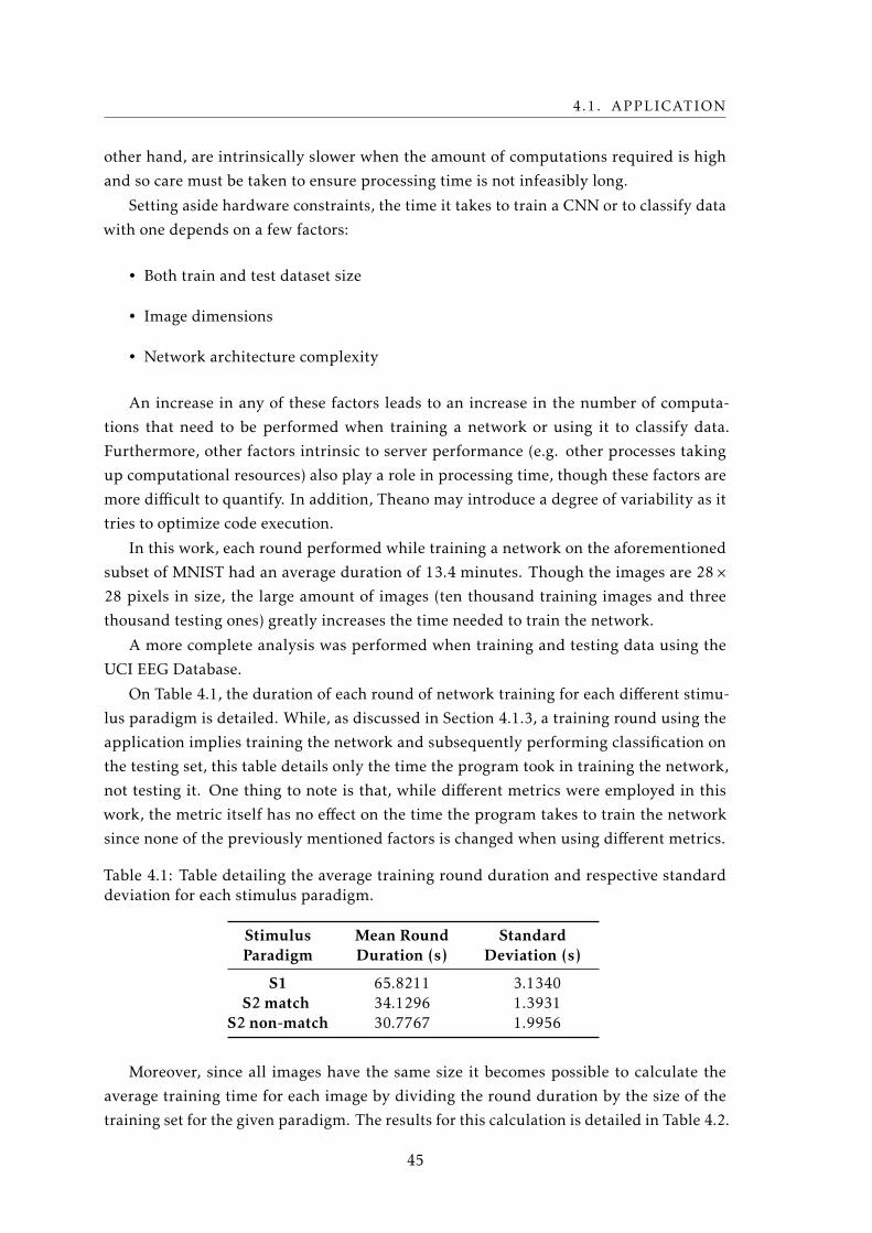
4.1. APPLICATION
other hand, are intrinsically slower when the amount of computations required is high
and so care must be taken to ensure processing time is not infeasibly long.
Setting aside hardware constraints, the time it takes to train a CNN or to classify data
with one depends on a few factors:
• Both train and test dataset size
• Image dimensions
• Network architecture complexity
An increase in any of these factors leads to an increase in the number of computa-
tions that need to be performed when training a network or using it to classify data.
Furthermore, other factors intrinsic to server performance (e.g. other processes taking
up computational resources) also play a role in processing time, though these factors are
more difficult to quantify. In addition, Theano may introduce a degree of variability as it
tries to optimize code execution.
In this work, each round performed while training a network on the aforementioned
subset of MNIST had an average duration of 13.4 minutes. Though the images are 28×28 pixels in size, the large amount of images (ten thousand training images and three
thousand testing ones) greatly increases the time needed to train the network.
A more complete analysis was performed when training and testing data using the
UCI EEG Database.
On Table 4.1, the duration of each round of network training for each different stimu-
lus paradigm is detailed. While, as discussed in Section 4.1.3, a training round using the
application implies training the network and subsequently performing classification on
the testing set, this table details only the time the program took in training the network,
not testing it. One thing to note is that, while different metrics were employed in this
work, the metric itself has no effect on the time the program takes to train the network
since none of the previously mentioned factors is changed when using different metrics.
Table 4.1: Table detailing the average training round duration and respective standarddeviation for each stimulus paradigm.
StimulusParadigm
Mean RoundDuration (s)
StandardDeviation (s)
S1 65.8211 3.1340S2 match 34.1296 1.3931
S2 non-match 30.7767 1.9956
Moreover, since all images have the same size it becomes possible to calculate the
average training time for each image by dividing the round duration by the size of the
training set for the given paradigm. The results for this calculation is detailed in Table 4.2.
45
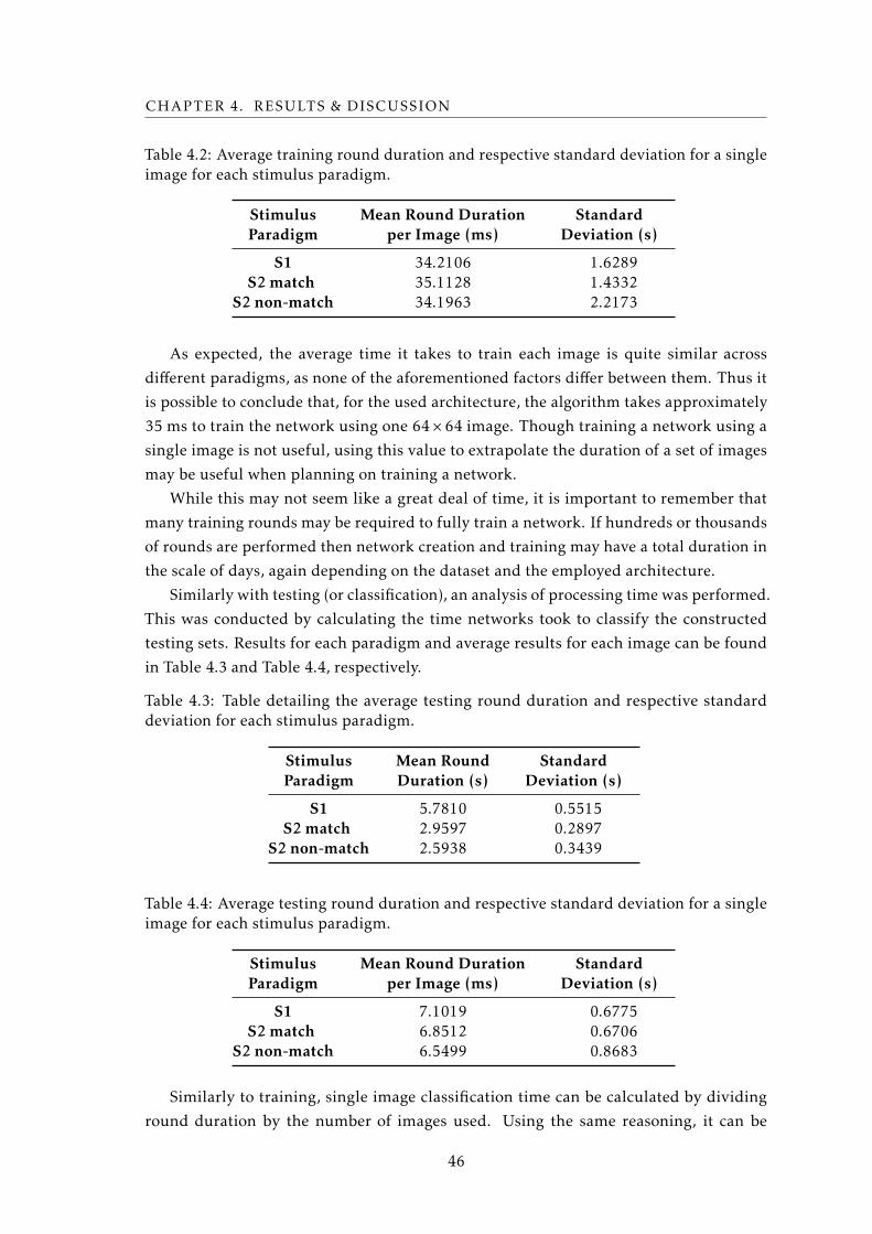
CHAPTER 4. RESULTS & DISCUSSION
Table 4.2: Average training round duration and respective standard deviation for a singleimage for each stimulus paradigm.
StimulusParadigm
Mean Round Durationper Image (ms)
StandardDeviation (s)
S1 34.2106 1.6289S2 match 35.1128 1.4332
S2 non-match 34.1963 2.2173
As expected, the average time it takes to train each image is quite similar across
different paradigms, as none of the aforementioned factors differ between them. Thus it
is possible to conclude that, for the used architecture, the algorithm takes approximately
35 ms to train the network using one 64× 64 image. Though training a network using a
single image is not useful, using this value to extrapolate the duration of a set of images
may be useful when planning on training a network.
While this may not seem like a great deal of time, it is important to remember that
many training rounds may be required to fully train a network. If hundreds or thousands
of rounds are performed then network creation and training may have a total duration in
the scale of days, again depending on the dataset and the employed architecture.
Similarly with testing (or classification), an analysis of processing time was performed.
This was conducted by calculating the time networks took to classify the constructed
testing sets. Results for each paradigm and average results for each image can be found
in Table 4.3 and Table 4.4, respectively.
Table 4.3: Table detailing the average testing round duration and respective standarddeviation for each stimulus paradigm.
StimulusParadigm
Mean RoundDuration (s)
StandardDeviation (s)
S1 5.7810 0.5515S2 match 2.9597 0.2897
S2 non-match 2.5938 0.3439
Table 4.4: Average testing round duration and respective standard deviation for a singleimage for each stimulus paradigm.
StimulusParadigm
Mean Round Durationper Image (ms)
StandardDeviation (s)
S1 7.1019 0.6775S2 match 6.8512 0.6706
S2 non-match 6.5499 0.8683
Similarly to training, single image classification time can be calculated by dividing
round duration by the number of images used. Using the same reasoning, it can be
46
4.1. APPLICATION
inferred that classifying a single 64× 64 image will take an average of approximately 7
ms.
This value is noticeably smaller than the average training time for one image, being
approximately one fifth of the duration. This is due to the fact that, in training, the
network must adjust its parameters.
It can therefore be concluded that, given the computational capabilities of the server
the application is housed in, it lacks in speed comparing to GPU-based programs [102],
especially in terms of network training. While it has been discussed in Section 4.1.8, it
is worthwhile to reiterate that the created application being housed on a Cloud server
means that it does not use resources that could be otherwise used for other tasks, i.e. it
works remotely and does not require a specific physical computer to be reserved to it.
As such, if there are no time constraints, longer processing time may be preferable to
reserving a computer or even having to acquire a GPU. Moreover, the fact that Cloud
servers are only billed while they are active may represent a more economical option in
the long run, as shutting down the server while not in use reduces expenditure.
It should however be noted that Cloud servers with access to GPUs exist in the market.
These allow to maintain the advantages of housing the application on a Cloud with the
added benefit of much faster processing, though they are naturally more expensive than
servers that do not have access to GPUs.
Fortunately, since Theano is compatible with both CPU and GPU, migrating the ap-
plication to an environment with the intention of using an available GPU would be as
simple as changing a configuration file for Theano to start using the GPU instead of the
CPU, thus showing the versatility of the created application.
With all that being said, while the developed application may not be ideal for creating
and training a new network when it comes to processing time, classifying data using a
trained network becomes more feasible. This can be explained by the fact that classifi-
cation does not entail multiple rounds, while training a network requires that several
iterations be performed. Using the obtained classification time per image value, it can be
calculated that in one hour it is possible to classify around half a million 64× 64 images
with the employed architecture. This shows that the application can be a powerful tool
to classify data when a network has already been trained. The fact that Caffe networks
can be uploaded to the server, as discussed in Section 4.1.4, and be converted so as to be
usable within the application is an attempt to bridge this gap, in the sense that trained net-
works can be uploaded to a remote environment that can be accessed when classification
is required.
Finally, it is important to mention that the effects of using different network architec-
tures were not analysed in this work. That being said, it follows from the same logic used
before that architectures with more layers and, overall, more computationally-intensive
layers (e.g. ones with smaller strides or larger filters) lead to an increase in processing
time in the same way as increasing the size of the training or testing sets. Due to the
need to perform several iterations when training, increasing network complexity will
47
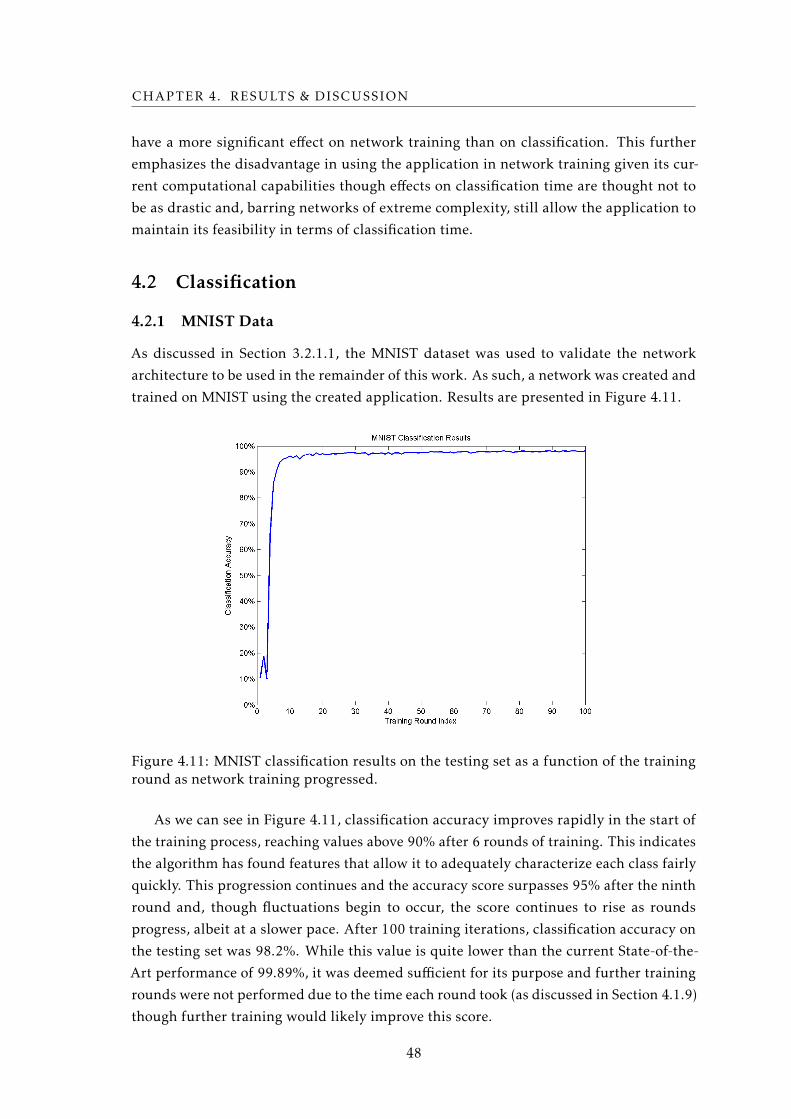
CHAPTER 4. RESULTS & DISCUSSION
have a more significant effect on network training than on classification. This further
emphasizes the disadvantage in using the application in network training given its cur-
rent computational capabilities though effects on classification time are thought not to
be as drastic and, barring networks of extreme complexity, still allow the application to
maintain its feasibility in terms of classification time.
4.2 Classification
4.2.1 MNIST Data
As discussed in Section 3.2.1.1, the MNIST dataset was used to validate the network
architecture to be used in the remainder of this work. As such, a network was created and
trained on MNIST using the created application. Results are presented in Figure 4.11.
Figure 4.11: MNIST classification results on the testing set as a function of the traininground as network training progressed.
As we can see in Figure 4.11, classification accuracy improves rapidly in the start of
the training process, reaching values above 90% after 6 rounds of training. This indicates
the algorithm has found features that allow it to adequately characterize each class fairly
quickly. This progression continues and the accuracy score surpasses 95% after the ninth
round and, though fluctuations begin to occur, the score continues to rise as rounds
progress, albeit at a slower pace. After 100 training iterations, classification accuracy on
the testing set was 98.2%. While this value is quite lower than the current State-of-the-
Art performance of 99.89%, it was deemed sufficient for its purpose and further training
rounds were not performed due to the time each round took (as discussed in Section 4.1.9)
though further training would likely improve this score.
48
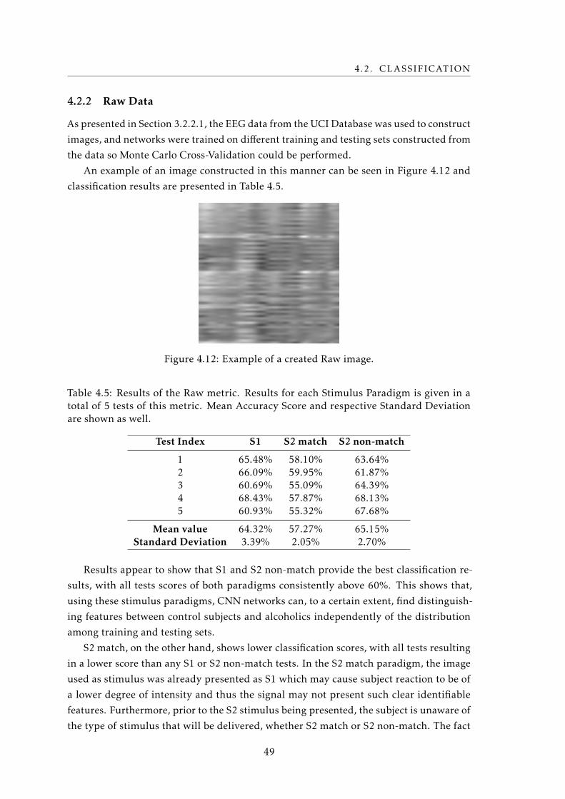
4.2. CLASSIFICATION
4.2.2 Raw Data
As presented in Section 3.2.2.1, the EEG data from the UCI Database was used to construct
images, and networks were trained on different training and testing sets constructed from
the data so Monte Carlo Cross-Validation could be performed.
An example of an image constructed in this manner can be seen in Figure 4.12 and
classification results are presented in Table 4.5.
Figure 4.12: Example of a created Raw image.
Table 4.5: Results of the Raw metric. Results for each Stimulus Paradigm is given in atotal of 5 tests of this metric. Mean Accuracy Score and respective Standard Deviationare shown as well.
Test Index S1 S2 match S2 non-match
1 65.48% 58.10% 63.64%2 66.09% 59.95% 61.87%3 60.69% 55.09% 64.39%4 68.43% 57.87% 68.13%5 60.93% 55.32% 67.68%
Mean value 64.32% 57.27% 65.15%Standard Deviation 3.39% 2.05% 2.70%
Results appear to show that S1 and S2 non-match provide the best classification re-
sults, with all tests scores of both paradigms consistently above 60%. This shows that,
using these stimulus paradigms, CNN networks can, to a certain extent, find distinguish-
ing features between control subjects and alcoholics independently of the distribution
among training and testing sets.
S2 match, on the other hand, shows lower classification scores, with all tests resulting
in a lower score than any S1 or S2 non-match tests. In the S2 match paradigm, the image
used as stimulus was already presented as S1 which may cause subject reaction to be of
a lower degree of intensity and thus the signal may not present such clear identifiable
features. Furthermore, prior to the S2 stimulus being presented, the subject is unaware of
the type of stimulus that will be delivered, whether S2 match or S2 non-match. The fact
49
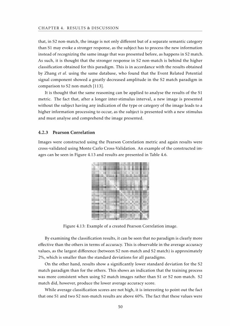
CHAPTER 4. RESULTS & DISCUSSION
that, in S2 non-match, the image is not only different but of a separate semantic category
than S1 may evoke a stronger response, as the subject has to process the new information
instead of recognizing the same image that was presented before, as happens in S2 match.
As such, it is thought that the stronger response in S2 non-match is behind the higher
classification obtained for this paradigm. This is in accordance with the results obtained
by Zhang et al. using the same database, who found that the Event Related Potential
signal component showed a greatly decreased amplitude in the S2 match paradigm in
comparison to S2 non-match [113].
It is thought that the same reasoning can be applied to analyse the results of the S1
metric. The fact that, after a longer inter-stimulus interval, a new image is presented
without the subject having any indication of the type or category of the image leads to a
higher information processing to occur, as the subject is presented with a new stimulus
and must analyse and comprehend the image presented.
4.2.3 Pearson Correlation
Images were constructed using the Pearson Correlation metric and again results were
cross-validated using Monte Carlo Cross-Validation. An example of the constructed im-
ages can be seen in Figure 4.13 and results are presented in Table 4.6.
Figure 4.13: Example of a created Pearson Correlation image.
By examining the classification results, it can be seen that no paradigm is clearly more
effective than the others in terms of accuracy. This is observable in the average accuracy
values, as the largest difference (between S2 non-match and S2 match) is approximately
2%, which is smaller than the standard deviations for all paradigms.
On the other hand, results show a significantly lower standard deviation for the S2
match paradigm than for the others. This shows an indication that the training process
was more consistent when using S2 match images rather than S1 or S2 non-match. S2
match did, however, produce the lower average accuracy score.
While average classification scores are not high, it is interesting to point out the fact
that one S1 and two S2 non-match results are above 60%. The fact that these values were
50
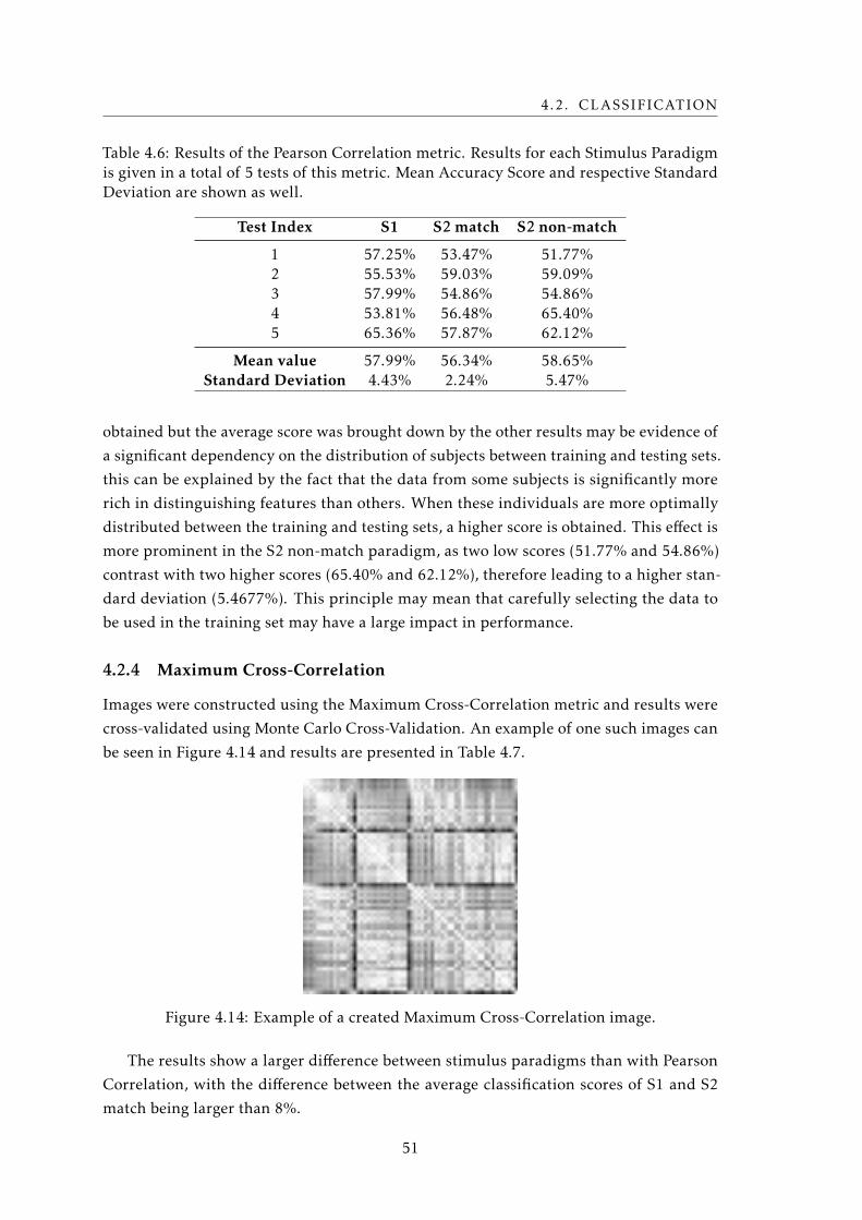
4.2. CLASSIFICATION
Table 4.6: Results of the Pearson Correlation metric. Results for each Stimulus Paradigmis given in a total of 5 tests of this metric. Mean Accuracy Score and respective StandardDeviation are shown as well.
Test Index S1 S2 match S2 non-match
1 57.25% 53.47% 51.77%2 55.53% 59.03% 59.09%3 57.99% 54.86% 54.86%4 53.81% 56.48% 65.40%5 65.36% 57.87% 62.12%
Mean value 57.99% 56.34% 58.65%Standard Deviation 4.43% 2.24% 5.47%
obtained but the average score was brought down by the other results may be evidence of
a significant dependency on the distribution of subjects between training and testing sets.
this can be explained by the fact that the data from some subjects is significantly more
rich in distinguishing features than others. When these individuals are more optimally
distributed between the training and testing sets, a higher score is obtained. This effect is
more prominent in the S2 non-match paradigm, as two low scores (51.77% and 54.86%)
contrast with two higher scores (65.40% and 62.12%), therefore leading to a higher stan-
dard deviation (5.4677%). This principle may mean that carefully selecting the data to
be used in the training set may have a large impact in performance.
4.2.4 Maximum Cross-Correlation
Images were constructed using the Maximum Cross-Correlation metric and results were
cross-validated using Monte Carlo Cross-Validation. An example of one such images can
be seen in Figure 4.14 and results are presented in Table 4.7.
Figure 4.14: Example of a created Maximum Cross-Correlation image.
The results show a larger difference between stimulus paradigms than with Pearson
Correlation, with the difference between the average classification scores of S1 and S2
match being larger than 8%.
51
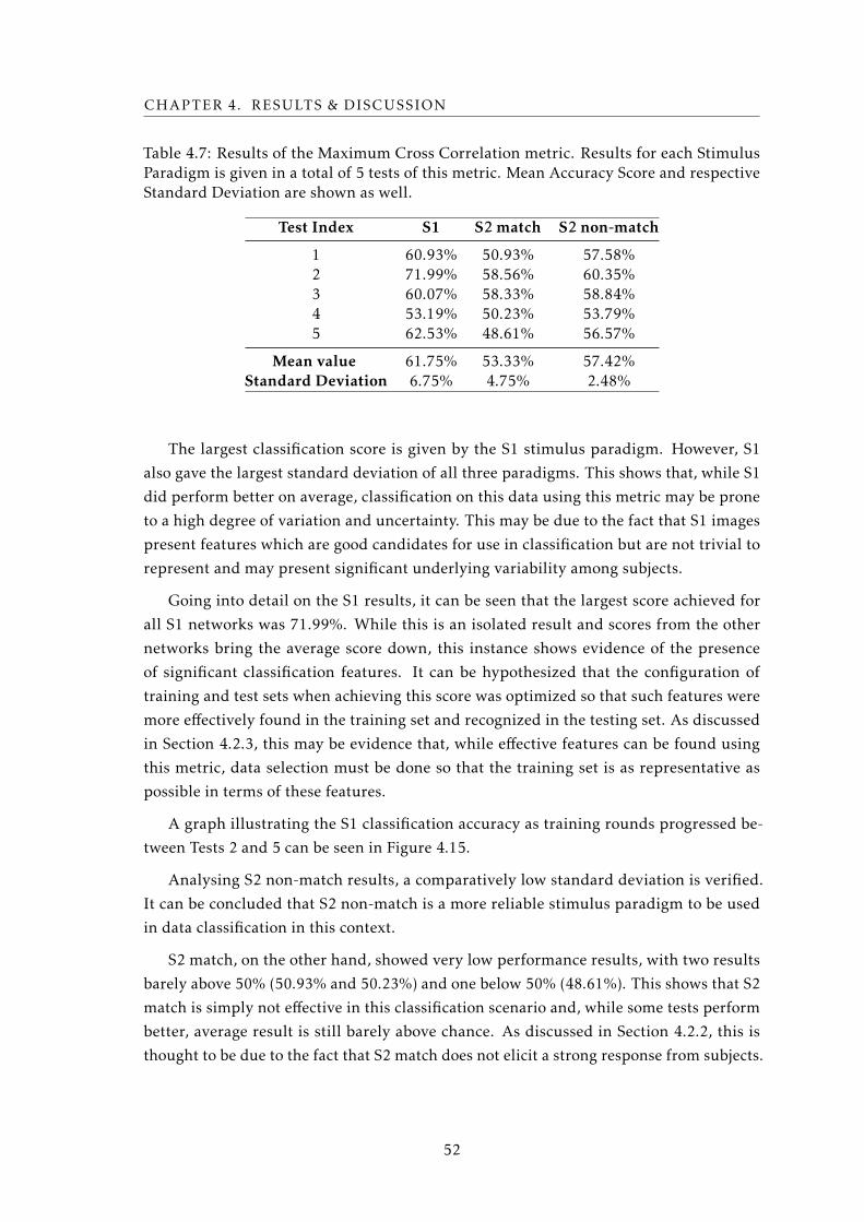
CHAPTER 4. RESULTS & DISCUSSION
Table 4.7: Results of the Maximum Cross Correlation metric. Results for each StimulusParadigm is given in a total of 5 tests of this metric. Mean Accuracy Score and respectiveStandard Deviation are shown as well.
Test Index S1 S2 match S2 non-match
1 60.93% 50.93% 57.58%2 71.99% 58.56% 60.35%3 60.07% 58.33% 58.84%4 53.19% 50.23% 53.79%5 62.53% 48.61% 56.57%
Mean value 61.75% 53.33% 57.42%Standard Deviation 6.75% 4.75% 2.48%
The largest classification score is given by the S1 stimulus paradigm. However, S1
also gave the largest standard deviation of all three paradigms. This shows that, while S1
did perform better on average, classification on this data using this metric may be prone
to a high degree of variation and uncertainty. This may be due to the fact that S1 images
present features which are good candidates for use in classification but are not trivial to
represent and may present significant underlying variability among subjects.
Going into detail on the S1 results, it can be seen that the largest score achieved for
all S1 networks was 71.99%. While this is an isolated result and scores from the other
networks bring the average score down, this instance shows evidence of the presence
of significant classification features. It can be hypothesized that the configuration of
training and test sets when achieving this score was optimized so that such features were
more effectively found in the training set and recognized in the testing set. As discussed
in Section 4.2.3, this may be evidence that, while effective features can be found using
this metric, data selection must be done so that the training set is as representative as
possible in terms of these features.
A graph illustrating the S1 classification accuracy as training rounds progressed be-
tween Tests 2 and 5 can be seen in Figure 4.15.
Analysing S2 non-match results, a comparatively low standard deviation is verified.
It can be concluded that S2 non-match is a more reliable stimulus paradigm to be used
in data classification in this context.
S2 match, on the other hand, showed very low performance results, with two results
barely above 50% (50.93% and 50.23%) and one below 50% (48.61%). This shows that S2
match is simply not effective in this classification scenario and, while some tests perform
better, average result is still barely above chance. As discussed in Section 4.2.2, this is
thought to be due to the fact that S2 match does not elicit a strong response from subjects.
52
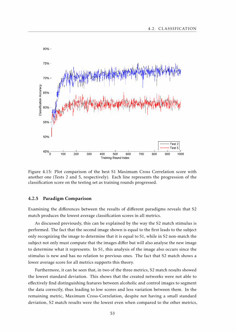
4.2. CLASSIFICATION
Figure 4.15: Plot comparison of the best S1 Maximum Cross Correlation score withanother one (Tests 2 and 5, respectively). Each line represents the progression of theclassification score on the testing set as training rounds progressed.
4.2.5 Paradigm Comparison
Examining the differences between the results of different paradigms reveals that S2
match produces the lowest average classification scores in all metrics.
As discussed previously, this can be explained by the way the S2 match stimulus is
performed. The fact that the second image shown is equal to the first leads to the subject
only recognizing the image to determine that it is equal to S1, while in S2 non-match the
subject not only must compute that the images differ but will also analyse the new image
to determine what it represents. In S1, this analysis of the image also occurs since the
stimulus is new and has no relation to previous ones. The fact that S2 match shows a
lower average score for all metrics supports this theory.
Furthermore, it can be seen that, in two of the three metrics, S2 match results showed
the lowest standard deviation. This shows that the created networks were not able to
effectively find distinguishing features between alcoholic and control images to segment
the data correctly, thus leading to low scores and less variation between them. In the
remaining metric, Maximum Cross-Correlation, despite not having a small standard
deviation, S2 match results were the lowest even when compared to the other metrics,
53
CHAPTER 4. RESULTS & DISCUSSION
thus further strengthening the given argument.
As for S1 and S2 non-match, it can be argued that the stimuli are quite similar. Both
involve presenting a new unseen image which is actively analysed by the subject. Thus, it
stands to reason that results between these paradigms are more similar than each of them
is to S2 match. However, one aspect must be taken into consideration: more S1 data was
used than S2 non-match, as discussed in Section 3.2.1.2. The fact that S2 non-match has
shown higher classification scores than S1 in two of the three employed metrics shows
evidence that the data used in this work was either sufficient in terms of quantity of
images used or was adequately representative of the intended features to achieve reliable
results.
Finally, whether S1 or S2 non-match was a more effective stimulus paradigm in classi-
fying the used data is debatable. While S2 non-match did produce higher scores in both
the Raw and Pearson Correlation metrics, S1 produced the highest single test score with
the Maximum Cross-Correlation metric, as well as the highest average score with the
same metric. It could be argued that the fact that, in S2 non-match, subjects have to press
a button using a randomly assigned hand per subject may lead to undesirable effects on
the acquired data. However, having the subject provide feedback from the stimulus may
lead to acquisition of data which simply is not present when the subject merely observes
the image.
In conclusion, no significant difference could be found to discern whether S1 or S2
non-match was a more effective stimulus paradigm for data acquisition to distinguish
alcoholics from controls in the scope of this work.
4.2.6 Metric Comparison
Results show that the Raw metric was the most effective of all the used metrics as it
produced the highest average classification scores in all stimulus paradigms. Standard
deviation was also, in general, lower for this metric.
For the Brain Connectivity metrics, it can be seen that higher average classification
scores were associated with higher standard deviations. This may be evidence that distin-
guishing features can be found with these metrics but may be strongly dependent on the
distribution of subjects between training and testing sets. As such, it may be theorized
that finding an optimal set distribution of subjects leads to an also optimal classification
score, as the optimized training set allows the network to be more adapted to find the
desired features. As the constructed datasets can be considered large in size, this can be
seen as a method of adapting the classifier to the data rather than the reverse. This is a
possible direction which can be taken to follow up on this work in the future.
Examining Equation (2.1) and Equation (2.2) brings to attention the fact that both
metrics possess the commutative property. Thus, due to the way the images were con-
structed, as presented in Section 3.2.2.2 and Section 3.2.2.3, they will present symmetry
along the diagonal that stretches from the top left corner to the bottom right corner of
54
4.2. CLASSIFICATION
the images. This effect can be observed in Figure 4.13 and Figure 4.14. It is debatable
whether this negatively affects classification. The fact that there is duplicated informa-
tion on the same image can be seen as undesirable simply due to redundancy but an
argument could be made that it is beneficial as it allows the network to view the same
data from different perspectives. In this scenario, each kernel in convolutional layers will
encounter the same information twice but since these kernels may not be symmetrical,
they will operate on the same data differently in both situations. This is analogue to Data
Augmentation methods such as horizontal flipping and rotation. These methods are used
to increase the amount of training data with new valid images and thereby making the
network generalize better to new data [117]. The difference in this case is the fact that
the original and augmented data are seen within the same image.
One important aspect to analyse is electrode order. Due to the fact that, in CNNs,
convolutional layers use locally connected moving filters to process data means that pix-
els located near one another will be processed differently than pixels which are located
further away from each other. As such, pixels in close proximity will be analysed for
features of lower dimensionality in the first Convolutional layers, such as edges. Convo-
lutional layers further down the architecture will analyse features of increasingly higher
dimensionality, such as texture. If the data in two pixels has a very low dimensionality
relationship, such as simple proportionality, having them far away from one another may
cause this relationship to not be found by the classifier. In real life images this is not
a problem since pixels which are far away from each other do not typically share low
dimensionality features but may both be integrated in a higher dimensionality aspect
which spans the distance between them, such as a pattern or texture. This is the basis for
the power of CNNs: the way the algorithm is adapted to find extremely complex features
with far reduced computational complexity when comparing to traditional ANNs. This,
of course, comes at the price of having local connectivity in Convolutional layers rather
than always having full connectivity with fully-connected layers [96].
In images which were constructed from non-visual data this is thought to be sig-
nificant in classification. While CNNs can identify complex relationships in the data,
the disposition of said data in the image can therefore be considered very important in
assuring the algorithm can correctly identify those relationships.
This argument can used to explain why the Raw metric performed better than the
Brain Connectivity metrics. The fact that, in the Raw images, each row represents the time
series for a single electrode means that each column provides a value which is temporally
sequential in regards to the adjacent columns. Although this denotes a temporal sequence
rather than a spatial one, it can be argued that such a relationship is similar to the spatial
proximity represented by pixels in, say, a photograph. As such, the CNN algorithm will
find features by analysing the relationship between electrodes in different moments of
time. To note that electrode ordering also plays a significant effect on the results of
this metric. To illustrate, a 3 × 3 filter in the first Convolutional layer will only analyse
electrodes which are within two indices apart in the electrode ordering, again due to local
55
CHAPTER 4. RESULTS & DISCUSSION
connectivity.
Experimenting with the order of electrodes can therefore be seen as a valid research
direction towards which this work could be continued. It can be argued that a valid
methodology with which the electrodes should be ordered for best results is to place
electrodes which are spatially closer in adjacent indices. However, due to the fact that
such an ordering would consist in a one-dimensional sequencing of a two-dimensional
arrangement of electrodes on the scalp, no clear disposition can be chosen without testing
different hypothesis.
Another possible solution which could be envisioned to tackle both the problem of
electrode disposition and the issue of redundant data also discussed in this work is to
design a more complex methodology of data arrangement within the image. Due to the
fact that the distance between data points in the image is relevant to feature detection, a
methodology which exploits this trait can be envisioned where data points are strategi-
cally placed so as to ensure the desired neighbouring pixels have relevant data in order
to improve classification. An example of this strategy would be to assign correlation
values constructed using electrodes sampled closer together to pixels at the centre of the
image. However, this is merely a conjecture which would have to be tested and many
other different methods could be proposed.
Another important aspect to be discussed is network architecture. The architecture
which was employed performed satisfyingly on the MNIST data. However, it failed to
perform in the same manner with the used metrics on the EEG data. For the architec-
ture to perform better on the MNIST is to be expected, as the handwritten digit images
represent far less complex data than those constructed using EEG data. Yet, whether
the used architecture was an inadequate representation of the capabilities of the CNN
algorithm is unlikely. It was to safeguard against this scenario that MNIST was used to
test classification performance with the architecture. Knowing the architecture worked
well on a common benchmarking dataset such as the MNIST is thought to be evidence
enough of the validity of the architecture for general image classification tasks. That
being said, it is certain that the employed architecture was not optimized to the type of
data to be classified. This is because the MNIST and the constructed EEG images repre-
sent data with completely different features and their optimized classification will most
certainly entail differing network architectures. Discovering what kind of architecture
would better fit the raw EEG and Brain Connectivity metrics was, however, beyond the
scope of this work.
From the obtained results it cannot be concluded that EEG and, more specifically,
Brain Connectivity are good metrics to classify AUD or, more broadly, neuropsychiatric
disorders using the methodology employed in this work.
It is thought that results obtained from the chosen metrics allow to conclude that
said metrics reveal features which can be used for classification. The reason to justify the
fact that more satisfying results were not not obtained lies in the aforementioned issues
underlying CNN classification.
56
Chapter
5Conclusions
5.1 Limitations
A number of limitations were presented in this work.
In the development of the application, the installation of Theano was the largest
obstacle that was faced. Online documentation on installing Theano proved to be scarce
and the available documentation was often incomplete or outdated. Furthermore, as
stated in Section 4.1.7, the fact that Theano is a low-level mathematical optimization
library and requires many low-level computations to be explicitly programmed led to a
steep learning curve in the development of the application. Combining that with the fact
that it had to be installed on a virtual machine further impeded development.
In terms of classification, the largest limitation proved to arise from the fact that the
application was housed on a Cloud environment without access to a GPU. This was due
to the Azure licence used. As discussed in Section 4.1.9, this led to the application having
high processing times when training networks and thus making it impractical to perform
a large number of different tests and therefore a more extensive research.
5.2 Future Work
Many directions can be envisioned to continue this work.
In terms of the development of the application, the use of a GPU in conjunction with
a Cloud environment is a definite step in the right direction in terms of fully combining
the strength of the CNN algorithm with the advantages of using a Cloud environment.
Furthermore, as discussed in Section 4.1.4, more specialized CNN features such as
Regularization techniques and different Score functions could be implemented as part of
the Network Customization feature. Adding this level of customization could go against
57
CHAPTER 5. CONCLUSIONS
the concept of minimalism associated with the application but finding a way to implement
these features and still retain the intuitiveness of the interface and structure can be
proposed as future work.
Moreover, expanding the compatibility with Caffe can be seen as a definite step for-
ward towards extending the versatility of the application. As this expansion in compat-
ibility entails that the application supports more layers and different features, this has
the additional effect of also expanding the application to be more complete in network
customization.
In terms of the application interface, adding the ability to plot the testing set classifi-
cation scores as training rounds progress can prove to be a significant improvement on
the user experience.
As mentioned, research as extensive as desired was not possible due to the limita-
tions faced. That being said and as discussed previously, many directions towards which
research can be taken were revealed during the course of this work.
These directions are based on varying the parameters of classification, the main of
which is the employed Image Construction Methodology. Varying this parameter entails
trying different Network Architectures, using new Brain Connectivity metrics and experi-
menting with the way images are constructed from the metrics. This last point is of great
interest since, as discussed previously, the CNN algorithm shows great promise if care is
taken in image construction. As such, ideas such as those proposed in Section 4.2.6 can
be employed to further research and better gauge the effectiveness of the CNN algorithm
in this situation.
5.3 Final Thoughts
When analysing the application, it is interesting to think of the possibilities such a pro-
gram can have in the context of improving healthcare. As the world converges into
on-demand technology and patient care is becoming evermore streamlined, accessible
and convenient, the way technologies are incorporated into both medical research and
patient care/diagnosis is experiencing change in a never before seen rate. Healthcare is,
in fact, more willing than ever to accept new technologies that improve all its processes.
The developed application is one such result of this revolution, bringing new concepts to
an ever-changing world.
To conclude, it is relevant to reiterate that the obtained classification results, while
not high enough to allow a definitive conclusion that the used metrics and methodology
represent a definite direction for research into neuropsychiatric disorder diagnosis, do
show indication that they can be used both in a research and clinical context, with more
tests being necessary. As such, the main contribution of this work lies in the analysis of
the obtained results and their discussion towards the creation of new directions to which
this research can be taken.
58
Bibliography
[1] P. Ampalam, S. Gunturu, and V. Padma, “A comparative study of caregiver burden
in psychiatric illness and chronic medical illness.”, Indian journal of psychiatry, vol.
54, no. 3, pp. 239–43, 2012.
[2] M. Duncan, L. Swartz, and H. Kathard, “The burden of psychiatric disability on
chronically poor households: Part 1 (costs)”, South African Journal of OccupationalTherapy, vol. 41, no. 3, pp. 55–63, 2011.
[3] M. Duncan, L. Swartz, and H. Kathard, “The burden of psychiatric disability on
chronically poor households: Part 2 (coping)”, South African Journal of Occupa-tional Therapy, vol. 41, no. 3, pp. 64–70, 2011.
[4] T. R. Insel, “Disruptive insights in psychiatry: Transforming a clinical discipline”,
Journal of Clinical Investigation, vol. 119, no. 4, pp. 700–705, 2009.
[5] G. Miller, “Mental health in developing countries. The unseen: mental illness’s
global toll.”, Science (New York, N.Y.), vol. 311, no. 5760, pp. 458–461, 2006.
[6] M. Ak, K. F. Yavuz, N. Lapsekili, and M. H. Türkçapar, “Evaluation of burden
in a group of patients with chronic psychiatric disorders and their caregivers”,
Dusunen Adam, vol. 25, no. 4, pp. 330–337, 2012.
[7] H. J. Watson, A. Swan, and P. R. Nathan, “Psychiatric diagnosis and quality of life:
The additional burden of psychiatric comorbidity”, Comprehensive Psychiatry, vol.
52, no. 3, pp. 265–272, 2011.
[8] H. U. Wittchen, F. Jacobi, J. Rehm, A. Gustavsson, M. Svensson, B. Jönsson, J. Ole-
sen, C. Allgulander, J. Alonso, C. Faravelli, L. Fratiglioni, P. Jennum, R. Lieb, A.
Maercker, J. van Os, M. Preisig, L. Salvador-Carulla, R. Simon, and H. C. Stein-
hausen, “The size and burden of mental disorders and other disorders of the brain
in Europe 2010”, Tech. Rep. 9, 2011, pp. 655–679.
[9] C. F. Reynolds, D. A. Lewis, T. Detre, A. F. Schatzberg, and D. J. Kupfer, “The
Future of Psychiatry as Clinical Neuroscience”, Academic Medicine, vol. 84, no. 4,
pp. 446–450, 2009.
[10] World Health Organization, “The Global Burden of Disease: 2004 update”, 2004Update, p. 146, 2008.
59
BIBLIOGRAPHY
[11] P. Bebbington, “The World Health Report 2001”, Social Psychiatry and PsychiatricEpidemiology, vol. 36, no. 10, pp. 473–474, 2001.
[12] K. Demyttenaere, R. Bruffaerts, J. Posada-Villa, et al., “Prevalence, severity, and
unmet need for treatment of mental disorders in the World Health Organization
World Mental Health Surveys.”, eng, JAMA, vol. 291, no. 21, pp. 2581–2590,
2004.
[13] American Psychiatric Association, Diagnostic and Statistical Manual of Mental Dis-orders, 5th ed. Washington, D.C., 2013, pp. 483–503.
[14] A. C. Altamura, M. Buoli, A. Caldiroli, L. Caron, C. Cumerlato Melter, C. Dobrea,
M. Cigliobianco, and F. Zanelli Quarantini, “Misdiagnosis, duration of untreated
illness (DUI) and outcome in bipolar patients with psychotic symptoms: A natu-
ralistic study”, Journal of Affective Disorders, vol. 182, pp. 70–75, 2015.
[15] K. McKenzie, “Moving the misdiagnosis debate forward”, International Review ofPsychiatry, vol. 11, pp. 153–161, 1999.
[16] S. M. Mirsattari, T. E. Gofton, and D. J. Chong, “Misdiagnosis of epileptic seizures
as manifestations of psychiatric illnesses.”, The Canadian Journal of NeurologicalSciences, vol. 38, no. 3, pp. 487–493, 2011.
[17] G. I. Van Schalkwyk, F. Peluso, Z. Qayyum, J. C. McPartland, and F. R. Volkmar,
“Varieties of Misdiagnosis in ASD: An Illustrative Case Series”, Journal of Autismand Developmental Disorders, vol. 45, no. 4, pp. 911–918, 2015.
[18] A. M. Erdozain and L. F. Callado, “Involvement of the endocannabinoid system
in alcohol dependence: The biochemical, behavioral and genetic evidence”, Drugand Alcohol Dependence, vol. 117, no. 2-3, pp. 102–110, 2011.
[19] World Health Organisation, “Global status report on alcohol and health 2014”,
Global status report on alcohol, pp. 1–392, 2014.
[20] D. M. Tomkins and E. M. Sellers, “Addiction and the brain: role of neurotransmit-
ters in the cause and treatment of drug dependance”, Canadian Medical AssociationJournal, vol. 164, no. 6, pp. 817–821, 2001.
[21] K. H. Taber, R. A. Hurley, and S. C. Yudofsky, “Diagnosis and treatment of neu-
ropsychiatric disorders.”, Annual review of medicine, vol. 61, pp. 121–33, 2010.
[22] A. M. Burhan, N. M. Marlatt, L. Palaniyappan, U. C. Anazodo, and F. S. Prato,
“Role of Hybrid Brain Imaging in Neuropsychiatric Disorders”, Diagnostics, vol. 5,
no. 4, pp. 577–614, 2015.
[23] E. Başar, “Brain oscillations in neuropsychiatric disease”, Dialogues in ClinicalNeuroscience, vol. 15, no. 3, pp. 291–300, 2013.
[24] R. Takizawa, M. Fukuda, S. Kawasaki, et al., “Neuroimaging-aided differential
diagnosis of the depressive state”, NeuroImage, vol. 85, pp. 498–507, 2014.
60
BIBLIOGRAPHY
[25] H. Lu and E. A. Stein, “Resting state functional connectivity: Its physiological
basis and application in neuropharmacology”, Neuropharmacology, vol. 84, pp. 79–
89, 2014.
[26] M. Kaiser, “A tutorial in connectome analysis: Topological and spatial features of
brain networks”, NeuroImage, vol. 57, no. 3, pp. 892–907, 2011.
[27] S. D. Keilholz, “The neural basis of time-varying resting-state functional connec-
tivity”, Brain connectivity, vol. 4, no. 10, pp. 769–779, 2014.
[28] A. M. Bastos and J.-M. Schoffelen, “A Tutorial Review of Functional Connectivity
Analysis Methods and Their Interpretational Pitfalls”, Frontiers in Systems Neuro-science, vol. 9, pp. 1–23, 2016.
[29] V. Sakkalis, “Review of advanced techniques for the estimation of brain connec-
tivity measured with EEG/MEG”, Computers in Biology and Medicine, vol. 41, no.
12, pp. 1110–1117, 2011.
[30] M. Teplan, “Fundamentals of EEG measurement”, Measurement Science Review,
vol. 2, no. 2, pp. 1–11, 2002.
[31] M. Bönstrup, R. Schulz, J. Feldheim, F. C. Hummel, and C. Gerloff, “Dynamic
causal modelling of EEG and fMRI to characterize network architectures in a
simple motor task”, NeuroImage, vol. 124, pp. 498–508, 2016.
[32] D. Brunet, M. M. Murray, and C. M. Michel, “Spatiotemporal analysis of multi-
channel EEG: CARTOOL”, Computational Intelligence and Neuroscience, vol. 2011,
pp. 1–15, 2011.
[33] A. Khanna, A. Pascual-Leone, C. M. Michel, and F. Farzan, “Microstates in resting-
state EEG: current status and future directions.”, Neuroscience and BiobehavioralReviews, vol. 49, pp. 105–13, 2015.
[34] S. Chanraud, A. L. Pitel, A. Pfefferbaum, and E. V. Sullivan, “Disruption of func-
tional connectivity of the default-mode network in alcoholism”, Cerebral Cortex,
vol. 21, no. 10, pp. 2272–2281, 2011.
[35] R. Cao, Z. Wu, H. Li, J. Xiang, and J. Chen, “Disturbed connectivity of EEG func-
tional networks in alcoholism: A graph-theoretic analysis”, Bio-Medical Materialsand Engineering, vol. 24, no. 6, pp. 2927–2936, 2014.
[36] N. Kannathal, U. R. Acharya, C. M. Lim, and P. K. Sadasivan, “Characterization of
EEG - A comparative study”, Computer Methods and Programs in Biomedicine, vol.
80, no. 1, pp. 17–23, 2005.
[37] S. Lemm, B. Blankertz, T. Dickhaus, and K. R. Müller, “Introduction to machine
learning for brain imaging”, NeuroImage, vol. 56, no. 2, pp. 387–399, 2011.
[38] I. Kononenko, “Machine learning for medical diagnosis: History, state of the art
and perspective”, Artificial Intelligence in Medicine, vol. 23, no. 1, pp. 89–109,
2001.
61

BIBLIOGRAPHY
[39] M. Seera, C. P. Lim, W. S. Liew, E. Lim, and C. K. Loo, “Classification of electrocar-
diogram and auscultatory blood pressure signals using machine learning models”,
Expert Systems with Applications, vol. 42, no. 7, pp. 3643–3652, 2015.
[40] P. Sajda, “Machine Learning for Detection and Diagnosis of Disease”, AnnualReview of Biomedical Engineering, vol. 8, no. 1, pp. 537–565, 2006.
[41] P. L. Peissig, V. Santos Costa, M. D. Caldwell, C. Rottscheit, R. L. Berg, E. A.
Mendonca, and D. Page, “Relational machine learning for electronic health record-
driven phenotyping”, Journal of Biomedical Informatics, vol. 52, pp. 260–270, 2014.
[42] G. Huang, G. B. Huang, S. Song, and K. You, “Trends in extreme learning ma-
chines: A review”, Neural Networks, vol. 61, pp. 32–48, 2015.
[43] K. Kourou, T. P. Exarchos, K. P. Exarchos, M. V. Karamouzis, and D. I. Fotiadis,
“Machine learning applications in cancer prognosis and prediction”, Computa-tional and Structural Biotechnology Journal, vol. 13, pp. 8–17, 2015.
[44] M. J. Patel, A. Khalaf, and H. J. Aizenstein, “Studying depression using imaging
and machine learning methods”, NeuroImage: Clinical, vol. 10, pp. 115–123, 2015.
[45] K. O’Shea and R. Nash, “An Introduction to Convolutional Neural Networks”,
CoRR, pp. 1–11, 2015.
[46] L. Wan, M. Zeiler, S. Zhang, Y. LeCun, and R. Fergus, “Regularization of neural
networks using dropconnect”, ICML, no. 1, pp. 109–111, 2013.
[47] L. A. Gatys, A. S. Ecker, and M. Bethge, “A Neural Algorithm of Artistic Style”,
arXiv preprint, pp. 3–7, 2015.
[48] H. A. Perlin and H. S. Lopes, “Extracting human attributes using a convolutional
neural network approach”, Pattern Recognition Letters, vol. 68, pp. 250–259, 2015.
[49] Y. Zhang, I. J. Marshall, and B. C. Wallace, “Rationale-Augmented Convolutional
Neural Networks for Text Classification”, CoRR, 2016.
[50] S. Ganapathy, K. Han, S. Thomas, M. Omar, M. V. Segbroeck, and S. S. Narayanan,
“Robust Language Identification Using Convolutional Neural Network Features”,
in Fifteenth Annual Conference of the International Speech Communication Associa-tion, 2014, pp. 1846–1850.
[51] Y. LeCun, Y. Bengio, and G. Hinton, “Deep learning”, Nature, vol. 521, no. 7553,
pp. 436–444, 2015.
[52] H. Cecotti and A. Graeser, “Convolutional Neural Network with embedded Fourier
Transform for EEG classification”, in 19th International Conference on PatternRecognition, 2008, pp. 1–4.
[53] H. Cecotti and A. Gräser, “Convolutional neural networks for P300 detection with
application to brain-computer interfaces”, IEEE Transactions on Pattern Analysisand Machine Intelligence, vol. 33, no. 3, pp. 433–445, 2011.
62
BIBLIOGRAPHY
[54] L. Ma, J. W. Minett, T. Blu, and W. S.-Y. Wang, “Resting State EEG-Based Biomet-
rics for Individual Identification Using Convolutional Neural Networks”, in IEEEEngineering in Medicine and Biology Society, 2015, pp. 2848–2851.
[55] Y. Zhao and L. He, “Deep Learning in the EEG Diagnosis of Alzheimer’s Disease”,
in Computer Vision - ACCV 2014 Workshops: Singapore, Singapore, November 1-2, 2014, Revised Selected Papers, Part I, C. V. Jawahar and S. Shan, Eds. Cham:
Springer International Publishing, 2015, pp. 340–353.
[56] W. Zhang, R. Li, H. Deng, L. Wang, W. Lin, S. Ji, and D. Shen, “Deep convolutional
neural networks for multi-modality isointense infant brain image segmentation”,
NeuroImage, vol. 108, pp. 214–224, 2015.
[57] J. Xu, X. Luo, G. Wang, H. Gilmore, and A. Madabhushi, “A Deep Convolutional
Neural Network for segmenting and classifying epithelial and stromal regions in
histopathological images”, Neurocomputing, vol. 191, pp. 214–223, 2016.
[58] A. Jamaludin, M. Lootus, T. Kadir, A. Zisserman, J. Urban, M. C. Battié, J. Fair-
bank, and I. McCall, “Automation of reading of radiological features from mag-
netic resonance images (MRIs) of the lumbar spine without human intervention
is comparable with an expert radiologist”, European Spine Journal, no. 7, 2017.
[59] P. Mirowski, D. Madhavan, Y. LeCun, and R. Kuzniecky, “Classification of patterns
of EEG synchronization for seizure prediction”, Clinical Neurophysiology, vol. 120,
no. 11, pp. 1927–1940, 2009.
[60] M. R. Nazari Kousarrizi, A. Asadi Ghanbari, A. Gharaviri, M. Teshnehlab, and M.
Aliyari, “Classification of alcoholics and non-alcoholics via EEG using SVM and
neural networks”, 3rd International Conference on Bioinformatics and BiomedicalEngineering, ICBBE 2009, pp. 1–4, 2009.
[61] A. Noblin, K. Cortelyou-Ward, and R. M. Servan, “Cloud Computing and Patient
Engagement”, The Journal of medical practice management, vol. 30, no. 2, pp. 65–70,
2014.
[62] G. Fernández-Cardeñosa, I. De La Torre-Díez, M. López-Coronado, and J. J.P. C.
Rodrigues, “Analysis of cloud-based solutions on EHRs systems in different sce-
narios”, Journal of Medical Systems, vol. 36, no. 6, pp. 3777–3782, 2012.
[63] L. Griebel, H.-U. Prokosch, F. Köpcke, D. Toddenroth, J. Christoph, I. Leb, I.
Engel, and M. Sedlmayr, “A scoping review of cloud computing in healthcare”,
BMC Medical Informatics and Decision Making, vol. 15, no. 1, p. 17, 2015.
[64] S. Pandey, W. Voorsluys, S. Niu, A. Khandoker, and R. Buyya, “An autonomic
cloud environment for hosting ECG data analysis services”, Future GenerationComputer Systems, vol. 28, no. 1, pp. 147–154, 2012.
[65] C. S. Reach, “Understanding Basic Elements of Cloud Operation”, DePaul Business& Commercial Law Journal, vol. 12, no. 4, pp. 411–419, 2014.
63
BIBLIOGRAPHY
[66] Q. F. Hassan, “Demystifying Cloud Security”, CrossTalk, pp. 16–21, 2011.
[67] M. D. Köhnke, “Approach to the genetics of alcoholism: A review based on patho-
physiology”, Biochemical Pharmacology, vol. 75, no. 1, pp. 160–177, 2008.
[68] A. Tseng, K. Nguyen, A. Hamid, M. Garg, P. Marquez, and K. Lutfy, “The role of
endogenous beta-endorphin and enkephalins in ethanol reward”, Neuropharma-cology, vol. 73, pp. 290–300, 2013.
[69] S. C. Pandey, “Neuronal signaling systems and ethanol dependence”, Molecularneurobiology, vol. 17, no. 1-3, pp. 1–15, 1998.
[70] I. Diamond and A. S. Gordon, “Cellular and molecular neuroscience of alco-
holism”, Physiological Reviews, vol. 77, no. 1, pp. 1–20, 1997.
[71] C. F. Valenzuela, “Alcohol and neurotransmitter interactions”, Alcohol health andresearch world, vol. 21, no. 2, pp. 144–148, 1997.
[72] D. L. Hodges, V. N. Kumar, and J. B. Redford, “Effects of alcohol on bone, muscle
and nerve.”, American family physician, vol. 34, no. 5, pp. 149–156, 1986.
[73] U. R. Acharya, S. V. Sree, S. Chattopadhyay, and J. S. Suri, “Automated diagnosis
of normal and alcoholic EEG signals.”, International journal of neural systems, vol.
22, no. 3, 2012.
[74] D. S. Hasin, C. P. O’Brien, M. Auriacombe, G. Borges, K. Bucholz, A. Budney,
W. M. Compton, T. Crowley, W. Ling, N. M. Petry, M. Schuckit, and B. F. Grant,
“DSM-5 criteria for substance use disorders: Recommendations and rationale”,
American Journal of Psychiatry, vol. 170, no. 8, pp. 834–851, 2013.
[75] E. Niedermeyer and F. H. L. Da Silva, Electroencephalography: basic principles, clin-ical applications, and related fields, English. Philadelphia: Lippincott Williams &
Wilkins, 2005.
[76] P. Olejniczak, “Neurophysiologic basis of EEG”, Journal of clinical neurophysiology:official publication of the American Electroencephalographic Society, vol. 23, no. 3,
pp. 186–189, 2006.
[77] R. M. Dondelinger, “Electroencephalographs”, Biomedical Instrumentation & Tech-nology, vol. 43, no. 5, pp. 388–391, 2009.
[78] “American Electroencephalographic Society guidelines for standard electrode po-
sition nomenclature.”, Journal of clinical neurophysiology : official publication of theAmerican Electroencephalographic Society, vol. 8, no. 2, pp. 200–202, 1991.
[79] A. B. Usakli, “Improvement of EEG signal acquisition: An electrical aspect for
state of the Art of front end”, Computational Intelligence and Neuroscience, vol.
2010, pp. 1–7, 2010.
[80] O. Sporns, “Network Analysis, Complexity, and Brain Function”, vol. 8, no. 1,
2003.
64
BIBLIOGRAPHY
[81] F Ferreira-Santos, “Complex Network Analysis of Brain Connectivity: An Intro-
duction”, University of Porto, Tech. Rep., 2012, pp. 3–11.
[82] O. Sporns and G. Tononi, “Classes of network connectivity and dynamics”, Com-plexity, vol. 7, no. 1, pp. 28–38, 2001.
[83] O. Sporns, “Structure and function of complex brain networks”, pp. 247–262,
2013.
[84] K. J. Friston, “Functional and Effective Connectivity in Neuroimaging : A Synthe-
sis”, vol. 78, 1994.
[85] E. W. Lang, A. M. Tomé, I. R. Keck, J. M. Górriz-Sáez, and C. G. Puntonet, “Brain
connectivity analysis: A short survey”, Computational Intelligence and Neuroscience,
vol. 2012, no. 3, 2012.
[86] B. Horwitz, “The elusive concept of brain connectivity”, NeuroImage, vol. 19, no.
2, pp. 466–470, 2003.
[87] C. M. J. Swinscow T.D.V., Statistics at Square One, 10th ed. BMJ Books, 2002.
[88] J. F. Kenney and E. S. Keeping, Mathematics of Statistics. 1962, vol. 1.
[89] E. M. Müller-Oehring, Y. C. Jung, A. Pfefferbaum, E. V. Sullivan, and T. Schulte,
“The resting brain of alcoholics”, Cerebral Cortex, vol. 25, no. 11, pp. 4155–4168,
2015.
[90] E. Shokri-Kojori, D. Tomasi, C. E. Wiers, G.-J. Wang, and N. D. Volkow, “Alcohol
affects brain functional connectivity and its coupling with behavior: greater effects
in male heavy drinkers”, Molecular Psychiatry, pp. 1–11, 2016.
[91] V. R. Preedy, Neuropathology of Drug Addictions and Substance Misuse. Volume 1:Foundations of Understanding, Tobacco, Alcohol, Cannabinoids and Opioids, 1st ed.
Elsevier Academic Press, 2016.
[92] S. Shalev-Shwartz and S. Ben-David, Understanding Machine Learning: From The-ory to Algorithms. New York, NY, USA: Cambridge University Press, 2014, pp. 1–
24.
[93] A. Smola and S. V. N Vishwanathan, Introduction to Machine Learning. Cambridge:
Cambridge University Press, 2008, pp. 1–12.
[94] C. M. Bishop, Neural Networks for Pattern Recognition. New York, NY, USA: Oxford
University Press, Inc., 1995.
[95] S. Woźniak, A.-D. Almási, V. Cristea, Y. Leblebici, and T. Engbersen, “Review of
Advances in Neural Networks: Neural Design Technology Stack”, Neurocomputing,
vol. 3, pp. 367–376, 2015.
[96] A. Karpathy, CS231n Convolutional Neural Networks for Visual Recognition, 2016.
[Online]. Available: http://cs231n.github.io/ (visited on 27/01/2016).
65
BIBLIOGRAPHY
[97] J. Schmidhuber, “Deep Learning in neural networks: An overview”, Neural Net-works, vol. 61, pp. 85–117, 2015.
[98] T. Schaul, I. Antonoglou, and D. Silver, “Unit Tests for Stochastic Optimization”,
ICLR, pp. 1–13, 2013.
[99] G. Hinton, N. Srivastava, and K. Swersky, Lecture 6.5-rmsprop: Divide the gradientby a running average of its recent magnitude, 2012.
[100] P. Mell and T. Grance, “The NIST Definition of Cloud Computing”, NIST SpecialPublication, vol. 145, pp. 2–3, 2011.
[101] B. G. Batista, J. C. Estrella, C. H. G. Ferreira, D. M. Leite Filho, L. H. V. Nakamura,
S. Reiff-Marganiec, M. J. Santana, and R. H. C. Santana, “Performance Evaluation
of Resource Management in Cloud Computing Environments”, PloS one, vol. 10,
no. 11, pp. 1–3, 2015.
[102] R. Al-Rfou, G. Alain, A. Almahairi, et al., “Theano: A Python framework for fast
computation of mathematical expressions”, arXiv e-prints, vol. abs/1605.0, 2016.
[103] G. Rossum, “Python Reference Manual”, Amsterdam, The Netherlands, Tech.
Rep., 1995.
[104] Y. Jia, E. Shelhamer, J. Donahue, S. Karayev, J. Long, R. Girshick, S. Guadarrama,
and T. Darrell, “Caffe: Convolutional Architecture for Fast Feature Embedding”,
arXiv preprint, 2014.
[105] Microsoft, Microsoft Azure. [Online]. Available: http://azure.microsoft.com
(visited on 20/04/2016).
[106] A. Ronacher, Flask (A Python Microframework). [Online]. Available: http://
flask.pocoo.org/ (visited on 21/04/2016).
[107] A. Ronacher, Jinja2. [Online]. Available: http://jinja.pocoo.org/ (visited on
21/04/2016).
[108] Y. LeCun, L. Bottou, Y. Bengio, and P. Haffner, “Gradient-based learning applied
to document recognition”, in Proceedings of the IEEE, 1998, pp. 2278–2324.
[109] Y. LeCun, C. Cortes, and C. Burges, The MNIST Database of handwritten digits.[Online]. Available: http://yann.lecun.com/exdb/mnist/ (visited on 21/04/
2016).
[110] D. Ciresan, U. Meier, and J. Schmidhuber, “Multi-column Deep Neural Networks
for Image Classification”, Cvpr, pp. 3642–3649, 2012.
[111] H. Begleiter, UCI EEG Database. [Online]. Available: https://kdd.ics.uci.
edu/databases/eeg/eeg.html (visited on 15/12/2016).
[112] G. V. Tcheslavski and F. F. Gonen, “Alcoholism-related alterations in spectrum,
coherence, and phase synchrony of topical electroencephalogram”, Computers inBiology and Medicine, vol. 42, no. 4, pp. 394–401, 2012.
66
BIBLIOGRAPHY
[113] X. L. Zhang, H. Begleiter, B. Porjesz, W. Wang, and A. Litke, “Event related po-
tentials during object recognition tasks”, Brain research bulletin, vol. 38, no. 6,
pp. 531–538, 1995.
[114] J. G. Snodgrass and M. Vanderwart, “A standardized set of 260 pictures: Norms for
name agreement, image agreement, familiarity, and visual complexity.”, Journalof Experimental Psychology: Human Learning & Memory, vol. 6, no. 2, pp. 174–215,
1980.
[115] A. Radford, Github - Theano-Tutorials. [Online]. Available: https://github.com/
Newmu/Theano-Tutorials (visited on 15/04/2016).
[116] Q.-S. Xu and Y.-Z. Liang, “Monte Carlo cross validation”, Chemometrics and Intel-ligent Laboratory Systems, vol. 56, no. 1, pp. 1–11, 2001.
[117] N. Takahashi, M. Gygli, B. Pfister, and L. Van Gool, “Deep Convolutional Neural
Networks and Data Augmentation for Acoustic Event Detection”, IEEE SignalProcessing Letters, pp. 1–5, 2016.
67


![[ em branco ] - da-ip.getmyip.comda-ip.getmyip.com/pdf/Old Publications/Portuguese/1968 - A Verdade... · 6 A VERDADE QUE CONDUZ A VIDA ETERNA fará com tôda a certeza, pois o Salmo](https://img.pdfslide.us/doc/110x75/5bebc80d09d3f2ff498ccda6/-em-branco-da-ip-publicationsportuguese1968-a-verdade-6-a-verdade.jpg)