I

Development of a Universal FE Model of a Cricket Ball

A thesis submitted in fulfilment of the requirements for the

degree of

Master of Engineering

Ning Cheng B.Eng. M.EnergySt

School of

Aerospace, Mechanical & Manufacturing Engineering

RMIT University

July 2008

II

DECLARATION

This is to certify that I, Ning CHENG, being a candidate for the degree of Master of

Mechanical Engineering (by research), am fully aware of the University of RMIT’s

rules and procedures relating to the preparation, submission, retention and use of

higher degree theses, and its policy on intellectual property.

I declare that:

(a) This thesis is my own composition;

(b) This thesis has not been submitted previously, in whole of in part, to qualify for

any other academic award;

(c) The content of the thesis is the result of work which has been carried out since the

official commencement date of the approved research program;

(d)Any editorial work in the thesis, paid or unpaid, carried out by a third party is

acknowledged;

(e) Ethics procedures and guidelines have been followed.

Signature …………………………………

Date ………………………………………

III

ACKNOWLEDGMENT

I would like to thank my supervisor, Dr. Monir Takla, for his expert guidance,

encouragement and patience throughout the course of my studies. His time and

support are greatly appreciated. I would also like to thank Professor Aleksandar Subic

for his very constructive comments on this paper.

My appreciation is also extended to Kookaburra Sports Co., Ltd for their generous

support on research materials. A special thanks to Professor Smith Lloyd (Washington

State University, USA) for his helpful comments and insights at various stages of this

research. I would also like to thank Mr. Peter Tkatchyk for his kind help during the

experimental studies.

Finally, I would thank my family including my Mum, Dad, and Grandma, thanks for

being such a great family. Christine, thank you so much for taking care of me and

encourage me throughout my studies, I feel so lucky to have such a great girl in my

life!

1

SUMMARY

In cricket, high speed impacts occur between the cricket ball and the bat, player and their

protective equipment. Improved understanding of impact dynamics has the potential to

significantly improve the development of cricket equipment and also contribute to

improving the player’s safety and performance. In particular, development of high

performance cricket balls with enhanced structural properties (e.g. improved durability)

would benefit greatly from such insight. In order to gain more insight into the impact

dynamics of cricket balls, appropriate structural models of the ball are required. This

work presents two fast-solving numerical models, a detailed multi-layer FE model as well

as a universal FE model, for the structural analysis of cricket balls. The models were

derived using experimental data obtained from tests developed for this purpose, including

drop tests and high speed impact tests.

The experimental work presented in this study included measurements of the impact

behaviour of two-layer, three-layer, and five-layer cricket balls using a dynamic signal

analyser and high speed video analysis software. The ball properties obtained

experimentally were used to develop two mathematical models: a single-element model

and a three-element model. These cricket ball models have been developed so that they

capture the key characteristics of ball-impact behaviour while allowing for fast-solving

dynamic simulation. The stiffness and damping properties of both models were

determined using a novel fast-solving genetic algorithm. These models predict the force-

time diagram during impact with very little computing cost. However, developing a

mathematical model with a reasonable level of accuracy is still a challenge. The

simulation of the ball model impact with a flat surface achieved reasonable agreement

with experimental results for both the single-element and the three-element models. The

genetic algorithm (GA) method proved to be more efficient and convenient than directly

solving the differential equations.

A detailed multi-layer, multi-material Finite Element (FE) model has also been developed.

The model has been experimentally validated and refined to a greater level of detail than

2

has been previously possible. Dynamic explicit analysis was conducted using ABAQUS

(ABAQUS Inc., USA). Rather than using the conventional trial-and-error approach for

model refinement, this study proposes a highly robust method to determine material

parameters that are extremely difficult to obtain by direct experimental measurement.

This approach incorporates several numerical methods, including FE simulation,

parameter optimization, and process automation.

A universal Finite Element (FE) ball model has also been developed within the ABAQUS

CAE environment. This model can be seen as a combination of an FE model template

and a material parameter selection tool based on an Artificial Neural Network (ANN)

model. This approach allows for rapid model development while producing accurate

results at different impact speeds. Two sets of real test data obtained from a five-layer

cricket ball and a two-layer cricket ball at impact velocity of 25 m/s were used to

examine the ANN model. Comparison of the results shows good agreement between the

simulation results and the experimental results. An important feature of the developed

universal FE model is its flexibility. The results show that the developed FE-ANN model

can be used to predict the impact behaviour of different types of cricket balls under

various dynamic conditions. This flexibility represents an advantage that can be utilized

by sports equipment developers to rapidly develop different cricket ball models needed

for inclusion in larger simulations involving impact of a cricket ball with other objects.

The developed FE-ANN model and the corresponding training process represent an

invaluable tool for facilitating design, analysis and structural optimization of cricket-

related sport equipment. Furthermore, the application presented here can be extended to

simulate any solid ball impact.

3

1. Introduction

1.1. Background

The materials used today to make cricket balls are mostly the same as in the 1770s. All

cricket balls are made from cork and latex rubber on the inside and leather on the outside.

In the past, research on sports balls usually concentrated on the effect of swing or

interaction of the ball with bat (Nicholls et al., 2005;Nathan, 2000;Sayers and Hill, 1999).

The structural behaviour of the ball itself attracted much less attention to date.

There is an increasing need in research and development for a theoretical cricket ball

model that can be incorporated in the analysis of bat impact stresses, deformations and

durability. Furthermore, with the growing concern for sports injuries, such a model would

also be used to improve the understanding of impact mechanisms between the cricket

ball, cricket player and their protective gear. This type of modelling would allow cost-

effective simulations of a range of impact events required in the development of

protective equipment, such as cricket helmets, face guards, gloves, etc.

A multi degrees of freedom theoretical cricket ball model, when included in relevant

numerical simulations involving different three-dimensional impact scenarios, should

enable prediction of energy exchange mechanisms between the striking bat, the protective

gear and the ball. It would also allow calculation of energy losses due to damping or

friction as well as analysis of stress distributions and time-dependent deformations.

Recently, advanced computer aided engineering (CAE) techniques have been widely

used in manufacturing sports equipment to enhance the quality of the sports equipment

produced and also to reduce the development time and cost. Due to the transient dynamic

nature of ball impact as well as the involved large deformations and non-linear behaviour,

transient dynamic finite element analysis (FEA) needs to be used. This is a powerful tool

4

that allows for the simulation of high speed impact events that occur over very short

periods of time. It also enables the analysis of three-dimensional structures, including

frictional effects and complex contact surfaces.

1.2. Objectives

The objectives of this study are:

1. to assemble and collate information regarding the application of modelling and

simulation technology for sports balls;

2. to design and to develop both static and dynamic experiments and to understand

the behavioural features of the specified cricket ball;

3. to develop two mathematical models of the cricket ball for theoretical and

comparative analysis;

4. to develop a detailed multi-layer and multi-material cricket ball model by using

the finite element method;

5. to build a universal, simplified FE model of a cricket ball with high accuracy and

low computing cost. This model can also been used for any other solid ball impact

simulation.

5

1.3. Thesis layout

Brief descriptions of each chapter of this thesis are listed below.

Chapter 1 provided the background to the game of cricket and discussed the importance

of cricket ball modelling. It also listed the objectives of this study.

Chapter 2 presents a literature review of relevant theoretical and experimental studies of

sports ball modelling techniques. This provides an overview of current sports ball model

simulations and experiments and shows how these have contributed to the experimental

design for this study.

Chapter 3 gives a detailed description of the experiments designed for this study and

explains the rationale for—as well as the assumptions, procedures and results of—the

experiments.

Chapter 4 shows how two mathematical models are developed for this study based on

MATLAB. Each set of modelling results is verified by comparing the modelling results

with the experimental results that were obtained in Chapter 3.

In Chapter 5, a completed FE model of a cricket ball is presented. This chapter

demonstrates how the model was developed and describes the processes of the selection

of the constitution equation, the determination of the material parameters, and the

verification of the model.

In Chapter 6, a universal FE model of the designated cricket ball is presented based on a

novel modelling system that was developed. This chapter gives a detailed description of

the construction of the novel modelling system, including descriptions of the

development of its methodology and its simulation results.

6

Chapter 7 compares all the models that have been developed in this study and

summarizes the actions and findings of this study.

Finally, Chapter 8 provides the conclusions of this study and gives suggestions for future

studies on sports ball modelling.

7

2. Literature Review

2.1. Introduction

Impact between a sports ball and a planar barrier has been widely investigated by

researchers using both theoretical modelling and experimental testing approaches

(Ujihashi et al., 2002;Cross, 1999). The review of research to date shows that baseball,

golf ball and tennis ball are the most common ball types investigated. The following

sections represent an overview of various theoretical models of sports balls for different

ball types in a chronological order.

Theoretical sports ball models have been generally classified into two main categories: (і)

mathematical models and (ii) numerical (mostly finite element) models. Mathematical

models have been quite popular and, due to their convenient features such as simplicity

and economical performance, they are still being used. The following sections discuss

both modelling methods in relation to the different ball types. The modelling

methodologies that are of particular interest to this study are highlighted.

Before adopting any of the computer-based models, it is necessary to conduct physical

experiments to calibrate or to verify the models. Therefore, in addition to modelling

studies, experimental investigations are also included in this literature review. These

published studies show that a range of methods that have been used in the past attempt to

obtain information regarding ball impact. These methods involved the use of cannon-gun

or pitching-machine projection, light gate, high speed camera, and speed measurement.

8

2.2. Sports ball impact mechanism

In order to successfully develop a cricket ball model, it is important to understand the

impact mechanism.

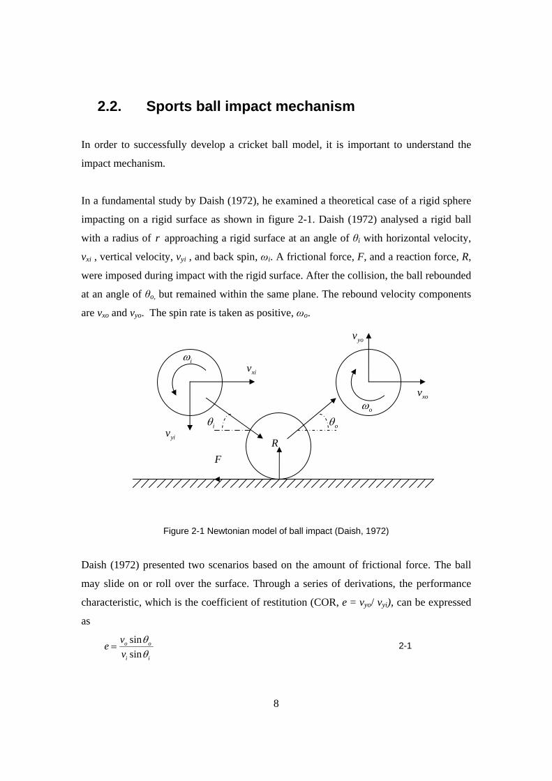
In a fundamental study by Daish (1972), he examined a theoretical case of a rigid sphere

impacting on a rigid surface as shown in figure 2-1. Daish (1972) analysed a rigid ball

with a radius of r approaching a rigid surface at an angle of θi with horizontal velocity,

vxi , vertical velocity, vyi , and back spin, ωi. A frictional force, F, and a reaction force, R,

were imposed during impact with the rigid surface. After the collision, the ball rebounded

at an angle of θo, but remained within the same plane. The rebound velocity components

are vxo and vyo. The spin rate is taken as positive, ωo.

Figure 2-1 Newtonian model of ball impact (Daish, 1972)

Daish (1972) presented two scenarios based on the amount of frictional force. The ball

may slide on or roll over the surface. Through a series of derivations, the performance

characteristic, which is the coefficient of restitution (COR, e = vyo/ vyi), can be expressed

as

sinsin

o o

i i

vev

θθ

= 2-1

F R yiv

xiv

xov

yov

iω

oω

iθ oθ

9

The post impact parameters can be written as

5 27

xi ixo

v rv ω−= 2-2

yo yiv ev= 2-3

and

5 27

xo xi io

v v rr r

ωω −= = 2-4

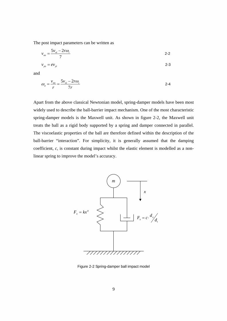
Apart from the above classical Newtonian model, spring-damper models have been most

widely used to describe the ball-barrier impact mechanism. One of the most characteristic

spring-damper models is the Maxwell unit. As shown in figure 2-2, the Maxwell unit

treats the ball as a rigid body supported by a spring and damper connected in parallel.

The viscoelastic properties of the ball are therefore defined within the description of the

ball-barrier “interaction”. For simplicity, it is generally assumed that the damping

coefficient, c, is constant during impact whilst the elastic element is modelled as a non-

linear spring to improve the model’s accuracy.

Figure 2-2 Spring-damper ball impact model

x

αkxFx = x

xt

dF c d= ⋅

m

10

Rate-independent parameters such as k and α, are typically derived from a quasi-static

compression test. The value of c could therefore be obtained by solving the equation of

motion numerically.

Furthermore, complicated spring-damper models, such as the combination of Maxwell or

Kelvin-Voigt units, involve several spring and/or damper elements connected either in

series or in parallel. Such models have been widely used for golf ball modelling

(Yamaguchi and Iwatsubo, 1998).

11

2.3. Golf ball modelling

A number of golf ball models with varied complexity, ranging from simple Newtonian

mechanics and non-linear spring-damper models (Ujihashi, 1994;Lieberman and

Johnson, 1994) to more sophisticated FE models (Ujihashi et al., 2002), have been

investigated.

One of the first mathematical models used to describe the impact between a golf ball and

a golf club was developed by Simon (1967). The differential equations used in the Simon

model are expressed as

1 2y y=& 2-5

32

2 1 2(1 )ky y ym

α= − +& 2-6

Where m is the mass of the golf ball, y1 is the deformation rate and y2 is the deformation

acceleration. The Simon model comprises two key parameters, k and α, which are

determined by fitting the predicted force versus time data to the measured force data.

This model predicts, with reasonable accuracy, the rebound velocities for two nominated

approaching velocities (120 ft/s, 140 ft/s). However, Johnson and Lieberman (1996) have

stated that there is a problem with the theoretical rounds due to the fact that this model

requires the deflection to be zero at the end of the impact, which proved to be inaccurate.

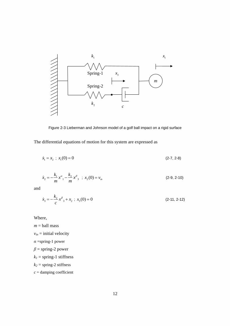
Lieberman and Johnson (1994) proposed a more complicated five-parameter spring-

damper golf model, as shown in figure 2-3. This model has been successfully used to

represent ball-barrier collisions over a wide range of approaching velocities.

12

Figure 2-3 Lieberman and Johnson model of a golf ball impact on a rigid surface

The differential equations of motion for this system are expressed as

1 2x x=& ; 1(0) 0x = (2-7, 2-8)

1 22 1 3

k kx x xm m

α β= − −& ; 2 (0) inx v= (2-9, 2-10)

and

23 3 2

kx x xc

β= − +& ; 3(0) 0x = (2-11, 2-12)

Where,

m = ball mass

vin = initial velocity

α =spring-1 power

β = spring-2 power

k1 = spring-1 stiffness

k2 = spring-2 stiffness

c = damping coefficient

m 3x

1x 1k

c 2k

Spring-1

Spring-2

13

Two rate-independent parameters, α and k1, are obtained from low speed compression

tests. The remaining three parameters, k2, c and β, are then derived from the recordings of

the impact forces using the gradient method.

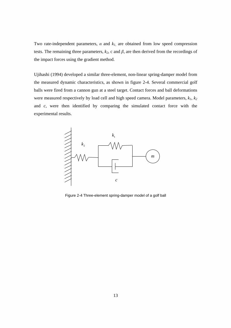
Ujihashi (1994) developed a similar three-element, non-linear spring-damper model from

the measured dynamic characteristics, as shown in figure 2-4. Several commercial golf

balls were fired from a cannon gun at a steel target. Contact forces and ball deformations

were measured respectively by load cell and high speed camera. Model parameters, k1, k2

and c, were then identified by comparing the simulated contact force with the

experimental results.

Figure 2-4 Three-element spring-damper model of a golf ball

1k

c

2k

m

14

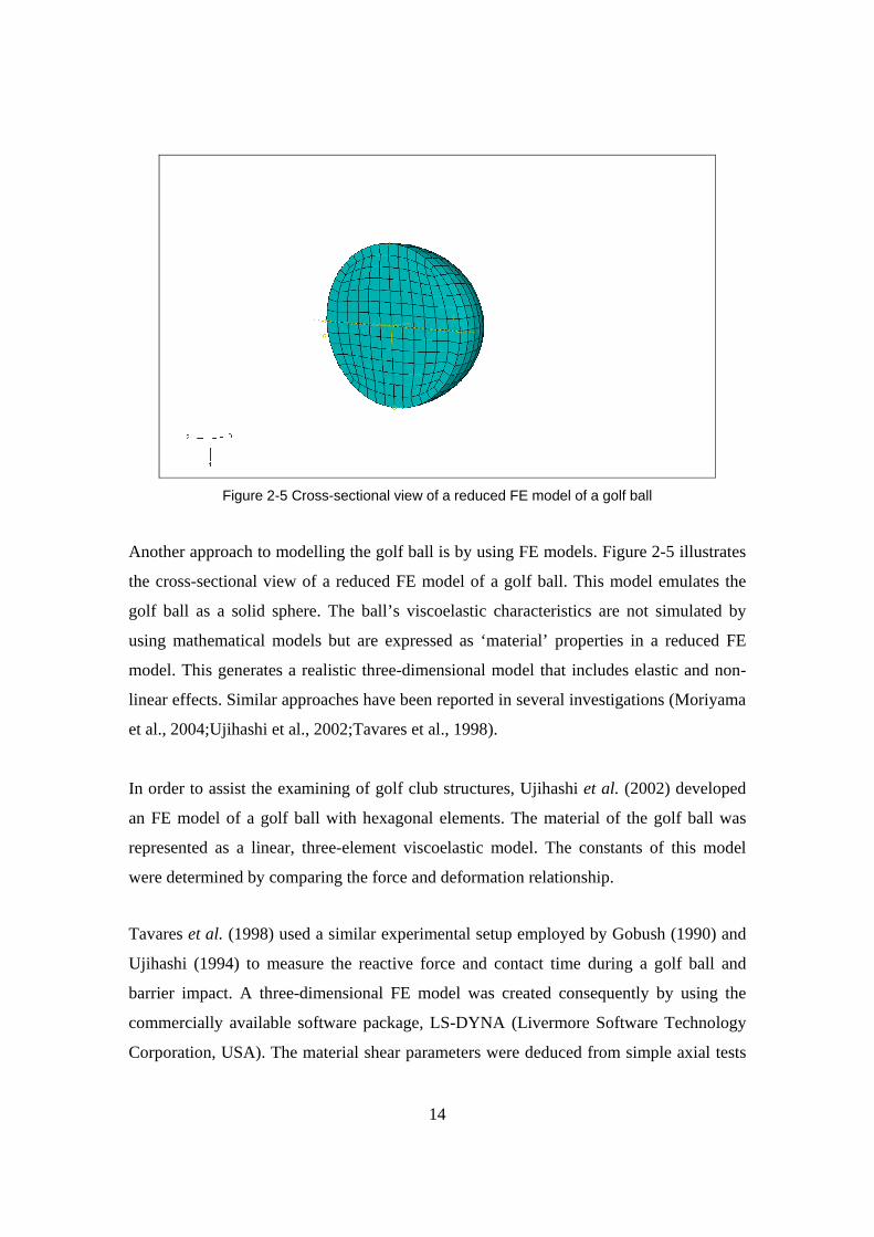
Figure 2-5 Cross-sectional view of a reduced FE model of a golf ball

Another approach to modelling the golf ball is by using FE models. Figure 2-5 illustrates

the cross-sectional view of a reduced FE model of a golf ball. This model emulates the

golf ball as a solid sphere. The ball’s viscoelastic characteristics are not simulated by

using mathematical models but are expressed as ‘material’ properties in a reduced FE

model. This generates a realistic three-dimensional model that includes elastic and non-

linear effects. Similar approaches have been reported in several investigations (Moriyama

et al., 2004;Ujihashi et al., 2002;Tavares et al., 1998).

In order to assist the examining of golf club structures, Ujihashi et al. (2002) developed

an FE model of a golf ball with hexagonal elements. The material of the golf ball was

represented as a linear, three-element viscoelastic model. The constants of this model

were determined by comparing the force and deformation relationship.

Tavares et al. (1998) used a similar experimental setup employed by Gobush (1990) and

Ujihashi (1994) to measure the reactive force and contact time during a golf ball and

barrier impact. A three-dimensional FE model was created consequently by using the

commercially available software package, LS-DYNA (Livermore Software Technology

Corporation, USA). The material shear parameters were deduced from simple axial tests

15

and the damping property was added empirically. The results of the simulation were

reported to be in good agreement with the experimental results.

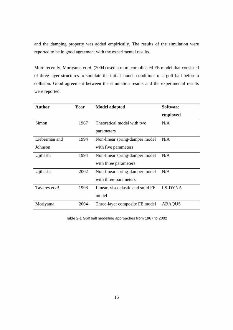
More recently, Moriyama et al. (2004) used a more complicated FE model that consisted

of three-layer structures to simulate the initial launch conditions of a golf ball before a

collision. Good agreement between the simulation results and the experimental results

were reported.

Author Year Model adopted Software

employed

Simon 1967 Theoretical model with two

parameters

N/A

Lieberman and

Johnson

1994 Non-linear spring-damper model

with five parameters

N/A

Ujihashi 1994 Non-linear spring-damper model

with three parameters

N/A

Ujihashi 2002 Non-linear spring-damper model

with three-parameters

N/A

Tavares et al. 1998 Linear, viscoelastic and solid FE

model

LS-DYNA

Moriyama 2004 Three-layer composite FE model ABAQUS

Table 2-1 Golf ball modelling approaches from 1967 to 2002

16

2.4. Tennis ball modelling

The interest in tennis ball modelling has grown since the first successful tennis ball model

was published by Daish (1972). Currently, a number of research projects have been

conducted in the area of tennis ball modelling.

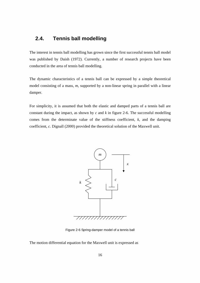
The dynamic characteristics of a tennis ball can be expressed by a simple theoretical

model consisting of a mass, m, supported by a non-linear spring in parallel with a linear

damper.

For simplicity, it is assumed that both the elastic and damped parts of a tennis ball are

constant during the impact, as shown by c and k in figure 2-6. The successful modelling

comes from the determinate value of the stiffness coefficient, k, and the damping

coefficient, c. Dignall (2000) provided the theoretical solution of the Maxwell unit.

Figure 2-6 Spring-damper model of a tennis ball

The motion differential equation for the Maxwell unit is expressed as

x

k c

m

17

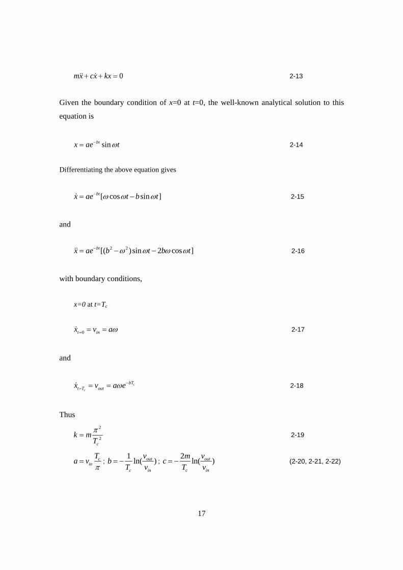
0mx cx kx+ + =&& & 2-13

Given the boundary condition of x=0 at t=0, the well-known analytical solution to this

equation is

sinbtx ae tω−= 2-14

Differentiating the above equation gives

[ cos sin ]btx ae t b tω ω ω−= −& 2-15

and

2 2[( )sin 2 cos ]btx ae b t b tω ω ω ω−= − −&& 2-16

with boundary conditions,

x=0 at t=Tc

0t inx v aω= = =& 2-17

and

c

c

bTt T outx v a eω −= = =& 2-18

Thus 2

2c

k mTπ

= 2-19

cin

Ta vπ

= ; 1 ln( )out

c in

vbT v

= − ; 2 ln( )out

c in

vmcT v

= − (2-20, 2-21, 2-22)

18

Where m= ball mass, vout = exit velocity, vin = initial velocity, and Tc = contact time.

Eventually, k and c could be calculated through cT , outv , and inv .

A further study by Kanda (2002) adopted an advanced FE model to study the tennis ball.

In his study, the rubber wall of the tennis ball was modelled using isoperimetric solid

elements and the pressurized gas in the ball was assumed to have the same properties as a

perfect gas.

Since the tennis ball has a different structure from that of other solid balls (golf balls,

baseballs, cricket balls), the detailed modelling techniques of tennis balls will not be

further discussed in this study.

2.5. Baseball modelling

Due to the structural similarities between the baseball and the cricket ball, it is important

to discuss baseball modelling methodologies.

A baseball is typically made up of multiple layers (a central cork or rubber core, wool

packing, and a stitched leather cover) and FE analysis has been used to evaluate baseball

performance at a very early stage in the history of such research into baseball

performance.

The first FE approximation for baseball behaviour during impact was made by Crisco et

al. (1997) using the elasticity theory. Crisco et al. (1997) assumed that the ball was a

homogeneous and linear elastic sphere with a COR of 1. Crisco et al. (1997) created this

model based on experimental axial compression tests in which one baseball was

compressed to 10% of its original diameter. Obviously, this model has limited

applicability to the dynamics of batted-ball impact as it fails to account for the non-

linearities associated with large deformations.

19

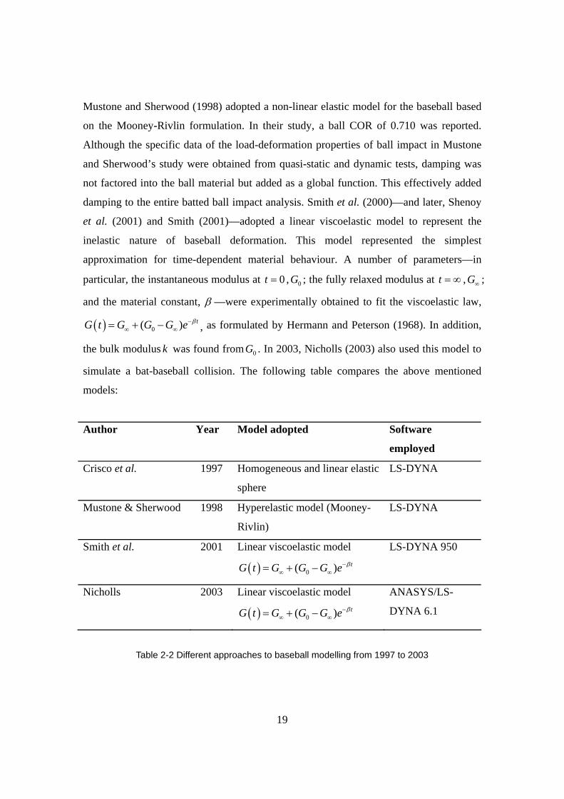
Mustone and Sherwood (1998) adopted a non-linear elastic model for the baseball based

on the Mooney-Rivlin formulation. In their study, a ball COR of 0.710 was reported.

Although the specific data of the load-deformation properties of ball impact in Mustone

and Sherwood’s study were obtained from quasi-static and dynamic tests, damping was

not factored into the ball material but added as a global function. This effectively added

damping to the entire batted ball impact analysis. Smith et al. (2000)—and later, Shenoy

et al. (2001) and Smith (2001)—adopted a linear viscoelastic model to represent the

inelastic nature of baseball deformation. This model represented the simplest

approximation for time-dependent material behaviour. A number of parameters—in

particular, the instantaneous modulus at 0t = , 0G ; the fully relaxed modulus at t = ∞ , G∞ ;

and the material constant, β —were experimentally obtained to fit the viscoelastic law,

( ) 0( ) tG t G G G e β−∞ ∞= + − , as formulated by Hermann and Peterson (1968). In addition,

the bulk modulus k was found from 0G . In 2003, Nicholls (2003) also used this model to

simulate a bat-baseball collision. The following table compares the above mentioned

models:

Author Year Model adopted Software

employed

Crisco et al. 1997 Homogeneous and linear elastic

sphere

LS-DYNA

Mustone & Sherwood 1998 Hyperelastic model (Mooney-

Rivlin)

LS-DYNA

Smith et al. 2001 Linear viscoelastic model

( ) 0( ) tG t G G G e β−∞ ∞= + −

LS-DYNA 950

Nicholls 2003 Linear viscoelastic model

( ) 0( ) tG t G G G e β−∞ ∞= + −

ANASYS/LS-

DYNA 6.1

Table 2-2 Different approaches to baseball modelling from 1997 to 2003

20

2.6. Softball modelling

Duris (2004) has conducted a series of tests on softballs to observe the COR and dynamic

compression in order to verify the two viscoelastic FE models that he created. The first

model used a power law expression with three parameters and the simulated results were

reported to be in good agreement with the experimental results. The second model

employed a material analysis technique called dynamic mechanical analysis (DMA). This

technique was used to identify the relaxation curve of the polyurethane foam core of the

softball. Subsequently, a Prony series model was fitted with the relaxation curve to

determine the parameters for the FE model. However, this method failed was unable to

predict the material parameters accurately.

2.7. Cricket ball modelling

The cricket ball is a complex non-homogeneous sphere made up of several layers of

different materials including cork-rubber core, cork-and-twine packing, and a stitched

leather. Review of published research shows that little work has been done to date on

cricket ball modelling. Two simplified cricket ball models were reported by Carré et al.

(2004) and Subic et al. (2005) respectively.

Carré et al. (2004) developed a single degree-of-freedom spring-damper model of a

cricket ball and simulated its impact with a rigid surface. Experimentally, the cricket ball

was dropped onto the horizontal flat top surface of a load cell from a range of different

heights to quantify the model’s dynamic stiffness and damping parameters. Although the

results from these simulations fit the experimental data with a reasonable degree of

accuracy, this model has several limitations. The first drawback is that the model is a

theoretical representation based on mathematical analysis, which makes it difficult to be

coupled with other existing FEA models. The second limitation is the fact that this is a

single degree-of-freedom model, which prevents its implementation in the simulation of

21

impact with three-dimensional objects. Finally, this model was developed under low

speed, which can hardly be used for the prediction of real game conditions in cricket.

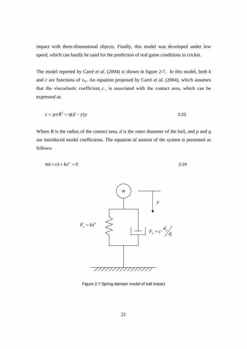
The model reported by Carré et al. (2004) is shown in figure 2-7. In this model, both k

and c are functions of vin. An equation proposed by Carré et al. (2004), which assumes

that the viscoelastic coefficient, c , is associated with the contact area, which can be

expressed as

2 ( )c p R q d y yπ= = − 2-23

Where R is the radius of the contact area, d is the outer diameter of the ball, and p and q

are introduced model coefficients. The equation of motion of the system is presented as

follows:

0mx cx kxα+ + =&& & 2-24

Figure 2-7 Spring-damper model of ball impact

y

yF kxα= y

yt

dF c d= ⋅

m

22

Where

m= ball mass

k=stiffness coefficient

α=spring power

c=damping coefficient

Subic et al. (2005) developed an approximate FE model to emulate the effects of the

interaction of the cricket ball with a rigid or deformable surface. Quasi-static axial

compression tests were first conducted on the entire ball under loading velocities varying

from 1 mm/min to 500 mm/min. The experimental results were extrapolated to predict

the performance of the ball at actual striking speeds used in standard tests (6.26 m/sec)

for cricket gear. An exponential relationship between the loading velocity and the ball

stiffness variable was found to prevail, which was used in the extrapolation. A numerical

model of the cricket ball was developed based on the concept of a soft surface encasing a

rigid body. The ball stiffness properties obtained from experimental tests were used to

calculate the properties of the soft surface of the ball, assuming homogeneous pressure

distribution over the contact area and neglecting the friction effect. To calculate the

pressure values from the experimentally measured forces values, the area of contact

between the ball surface and the anvils of the drop test machine was estimated as a

function of displacement. The non-linear ball stiffness characteristic was finally

calculated as a relationship between the contact pressure and the radial deformation of the

soft surface of the ball.

Even though this modelling approach significantly reduced the complexity of the finite

element modelling, it still has some inherent limitations. For example, in a simple

compression test the ball is subjected to pressures from both sides, which is different

from real application. Also, this model has not been verified through high speed dynamic

testing.

23

2.8. Summary

After reviewing the available literature on sports ball modelling, it can be seen that

accurate modelling of the dynamic behaviour of a cricket ball is a complex task due to the

ball’s complicated structure. Researchers have attempted to use different models to

describe different types of sports ball. Different approaches—from the simplest spring-

damper models to more sophisticated FE models—have been invented to describe and to

predict the dynamic behaviour of ball-barrier impacts. In particular, over the last few

decades, with the growing demand for engineering simulation, FE models are seen as a

potential replacement for spring-damper models. Sophisticated models share some

common features: they take into account energy loss during an impact; they express the

non-linear behaviour of a ball under high-velocity impact; and they describe viscoelastic

behaviour (Ujihashi, 1994).

However, a number of key issues are currently restricting sports ball modelling

developments. These are listed below:

1. Mathematical models with limited applicability are still being used in sports ball

modelling, for example, in cricket ball modelling.

2. To reduce the effort needed for FE modelling, simplified construction and simple

materials are used. This usually means that some crucial features of the actual ball

cannot be taken into account.

3. Key material parameters are not accurately defined in existing sports ball models.

Material parameters are often obtained through trial-and-error methods.

24

3. Experimental Testing of Ball Behaviour

3.1. Introduction

Prior to model development, experiments were designed and carried out to investigate the

impact behaviour of the cricket ball in order to establish a benchmark that can be used to

validate the developed ball model.

Generally, the apparatus used for the experiments consisted of a load cell mounted on a

heavy brass rod and a speed gate. To obtain a suitable ball speed for testing, the ball can

be dropped from a predetermined height (Carré et al., 2004) or it can be fired through a

cannon gun or a pitching machine (Moriyama et al., 2004;Smith et al., 2000). The major

difference between the cannon gun and the pitching machine is that the cannon gun does

not impart any spin to the ball while the pitching machine does. If a speed gate is difficult

to obtain, a high speed camera can be used as a substitute.

A basic understanding of the impact properties of a cricket ball is required to create a

precise model. In this study, two types of experiments were conducted: the drop test and

the high speed impact test. Three types of Kookaburra cricket balls were examined: a

two-layer solid ball, a three-layer ball and a five-layer ball. Each ball was tested over a

speed range of 5m/s to 25 m/s.

25

3.2. The drop tests

3.2.1.Test installation

The primary objective of the experiment is to measure the low speed contact force, the

coefficient of restitution (COR) and contact duration when the cricket ball impacts the

rigid surface. In this case, a range of dropping heights (0.38m-4.90m) were used to allow

the ball to reach a maximum speed of about 10m/s. The rig was designed with PCB pipes

connected to a vacuum pump. The height-adjustable rig released the ball from a range of

different heights. Other auxiliary equipment such as an impact cap, a mounting stud and a

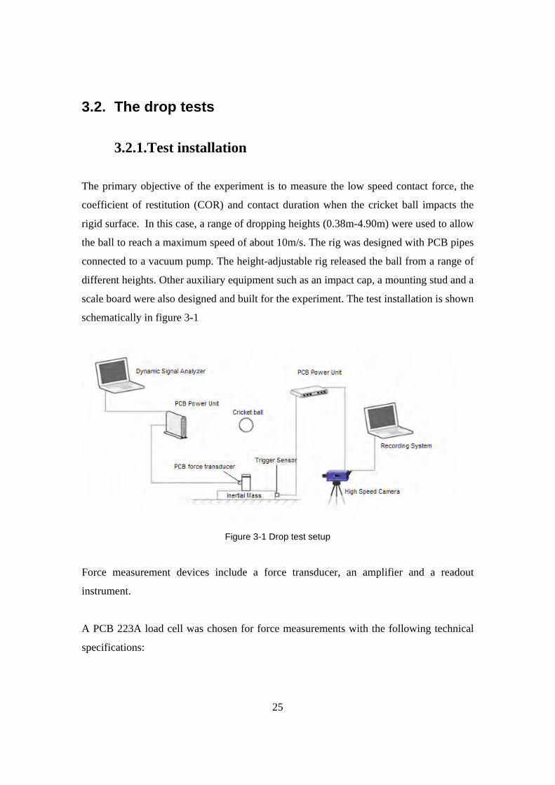
scale board were also designed and built for the experiment. The test installation is shown

schematically in figure 3-1

Figure 3-1 Drop test setup

Force measurement devices include a force transducer, an amplifier and a readout

instrument.

A PCB 223A load cell was chosen for force measurements with the following technical

specifications:

26

Sensitivity (± 15 %) 94.42 mV/kN

Measurement Range (Compression) 53.38 kN

Non-Linearity ≤ 1 % FS

Upper Frequency Limit 10 kHz

The calibration of the force transducer was obtained by integrating the impact force over

the contact time which allows comparison with the momentum change of the ball

according to the following equation:

1 2( )F dt m v v= −∫ 3-1

Where 1v and 2v is the ball-speed just before and just after the ball’s impact with the rigid

surface.

A PCB-482A16 charge amplifier was used with its gain value set to 10, which allowed

for the output voltage to be increased to 0.09 mV/N. The amplified signal was then

recognized by OROS OR25 pc-pack system and thus recorded by OR763 software

(OROS Corporation). Figure 3-2 is a screenshot of the software recording an impact force

pulse. The data sampling rate was set at 1 kHz due to the limitation of the data acquisition

system.

27

Figure 3-2 Screenshot of OR763 software recording of impact force pulse

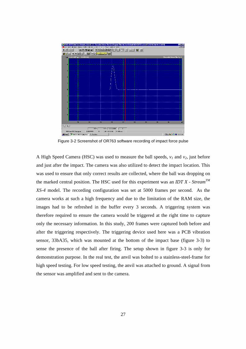
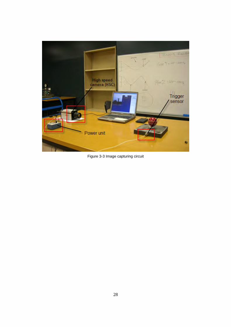
A High Speed Camera (HSC) was used to measure the ball speeds, v1 and v2, just before

and just after the impact. The camera was also utilized to detect the impact location. This

was used to ensure that only correct results are collected, where the ball was dropping on

the marked central position. The HSC used for this experiment was an IDT X - StreamTM

XS-4 model. The recording configuration was set at 5000 frames per second. As the

camera works at such a high frequency and due to the limitation of the RAM size, the

images had to be refreshed in the buffer every 3 seconds. A triggering system was

therefore required to ensure the camera would be triggered at the right time to capture

only the necessary information. In this study, 200 frames were captured both before and

after the triggering respectively. The triggering device used here was a PCB vibration

sensor, 33bA35, which was mounted at the bottom of the impact base (figure 3-3) to

sense the presence of the ball after firing. The setup shown in figure 3-3 is only for

demonstration purpose. In the real test, the anvil was bolted to a stainless-steel-frame for

high speed testing. For low speed testing, the anvil was attached to ground. A signal from

the sensor was amplified and sent to the camera.

28

Figure 3-3 Image capturing circuit

29

3.2.2.Data processing

Ten complete sets of experimental results were successfully obtained, one set of which

was selected for the purpose of verifying previously published findings. When the ball is

dropped onto the anvil, it experiences a vertical impulsive force:

dvF mdt

= 3-2

where v= dy /dt is the velocity of the ball’s centre of mass and y is the displacement of its centre

of mass.

Since the vertical impulse force during impact is normally of a much higher order than

the gravitational force, gravity effects can be neglected. For a measured force wave-form,

the y displacement can be obtained by solving the differential equation: 2

2 ( ) /d y F t mdt

= 3-3

with initial conditions

y =0 and 1dy vdt

= at t =0

As the measured force wave was stored in WAV format, it had to be exported for further

analysis. The exported WAV file was then converted by ORIGIN PRO 7.5 (OriginLab

Inc., USA) software into a binary format. Consequently, the binary file was used for

curve fitting using MATLAB 2006a (Mathworks Inc., USA). Impact and rebound speeds

were determined by dividing the vertical distance by the elapsed time, as shown in figure

3-4 below.

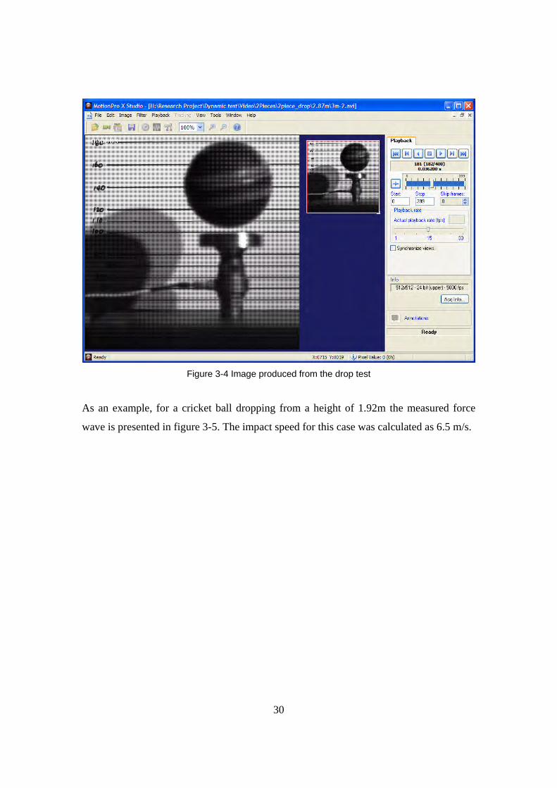
30

Figure 3-4 Image produced from the drop test

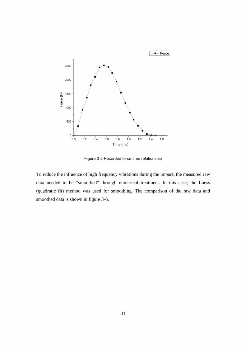
As an example, for a cricket ball dropping from a height of 1.92m the measured force

wave is presented in figure 3-5. The impact speed for this case was calculated as 6.5 m/s.

31

Figure 3-5 Recorded force-time relationship

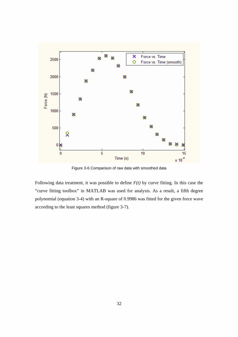
To reduce the influence of high frequency vibrations during the impact, the measured raw

data needed to be “smoothed” through numerical treatment. In this case, the Loess

(quadratic fit) method was used for smoothing. The comparison of the raw data and

smoothed data is shown in figure 3-6.

32

Figure 3-6 Comparison of raw data with smoothed data

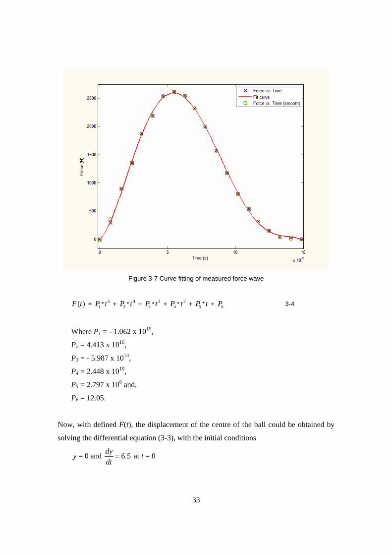
Following data treatment, it was possible to define F(t) by curve fitting. In this case the

“curve fitting toolbox” in MATLAB was used for analysis. As a result, a fifth degree

polynomial (equation 3-4) with an R-square of 0.9986 was fitted for the given force wave

according to the least squares method (figure 3-7).

33

Figure 3-7 Curve fitting of measured force wave

( )F t = 1P * 5t + 2P * 4t + 3P * 3t + 4P * 2t + 5P * t + 6P 3-4

Where P1 = - 1.062 x 1019,

P2 = 4.413 x 1016,

P3 = - 5.987 x 1013,

P4 = 2.448 x 1010,

P5 = 2.797 x 106 and,

P6 = 12.05.

Now, with defined F(t), the displacement of the centre of the ball could be obtained by

solving the differential equation (3-3), with the initial conditions

y = 0 and 6.5dydt

= at t = 0

34

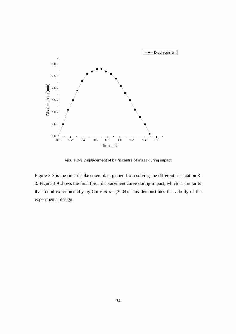
Figure 3-8 Displacement of ball’s centre of mass during impact

Figure 3-8 is the time-displacement data gained from solving the differential equation 3-

3. Figure 3-9 shows the final force-displacement curve during impact, which is similar to

that found experimentally by Carré et al. (2004). This demonstrates the validity of the

experimental design.

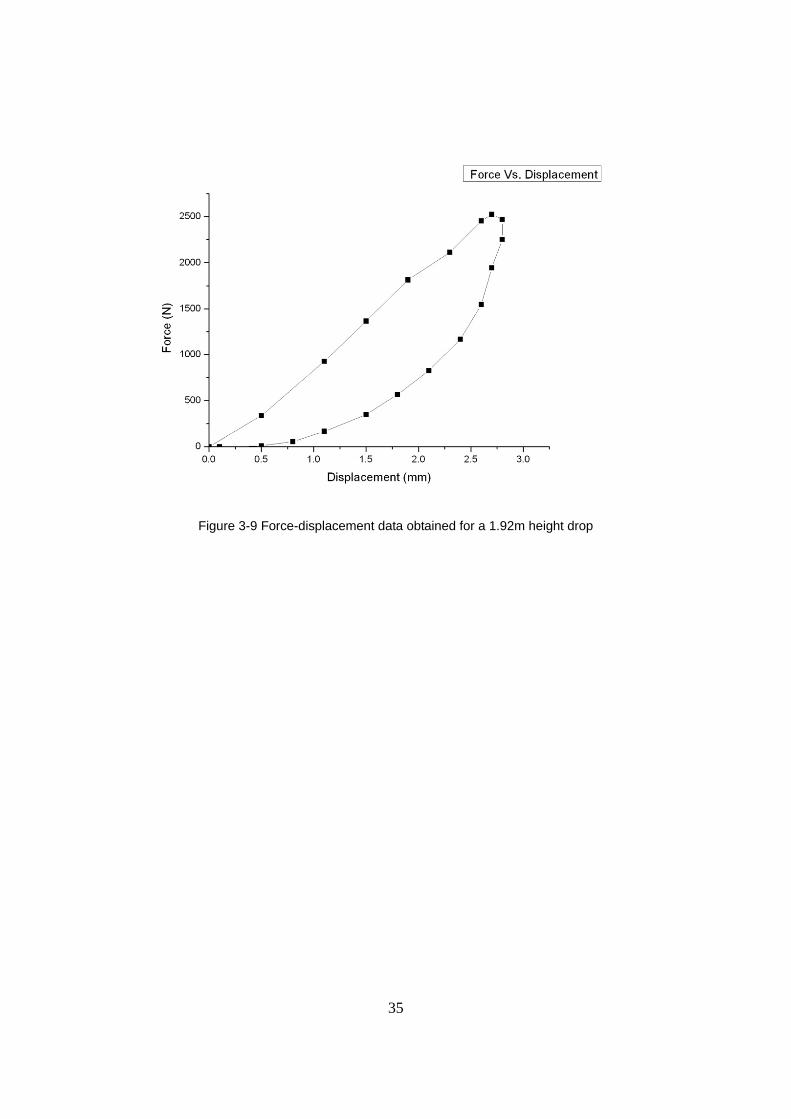
35

Figure 3-9 Force-displacement data obtained for a 1.92m height drop

36

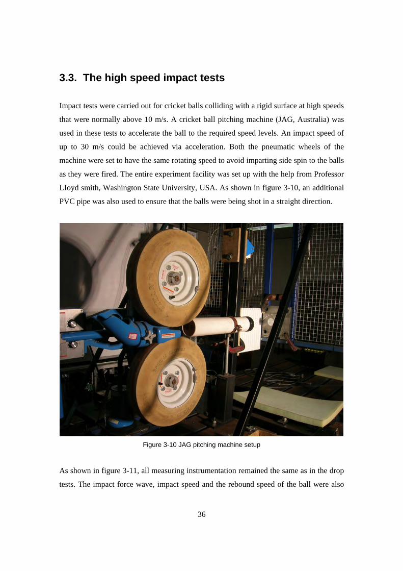
3.3. The high speed impact tests

Impact tests were carried out for cricket balls colliding with a rigid surface at high speeds

that were normally above 10 m/s. A cricket ball pitching machine (JAG, Australia) was

used in these tests to accelerate the ball to the required speed levels. An impact speed of

up to 30 m/s could be achieved via acceleration. Both the pneumatic wheels of the

machine were set to have the same rotating speed to avoid imparting side spin to the balls

as they were fired. The entire experiment facility was set up with the help from Professor

LIoyd smith, Washington State University, USA. As shown in figure 3-10, an additional

PVC pipe was also used to ensure that the balls were being shot in a straight direction.

Figure 3-10 JAG pitching machine setup

As shown in figure 3-11, all measuring instrumentation remained the same as in the drop

tests. The impact force wave, impact speed and the rebound speed of the ball were also

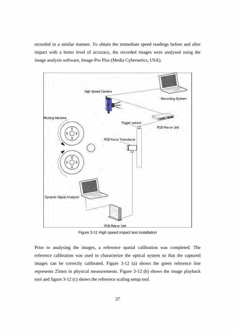
37

recorded in a similar manner. To obtain the immediate speed readings before and after

impact with a better level of accuracy, the recorded images were analysed using the

image analysis software, Image-Pro Plus (Media Cybernetics, USA).

Figure 3-11 High speed impact test installation

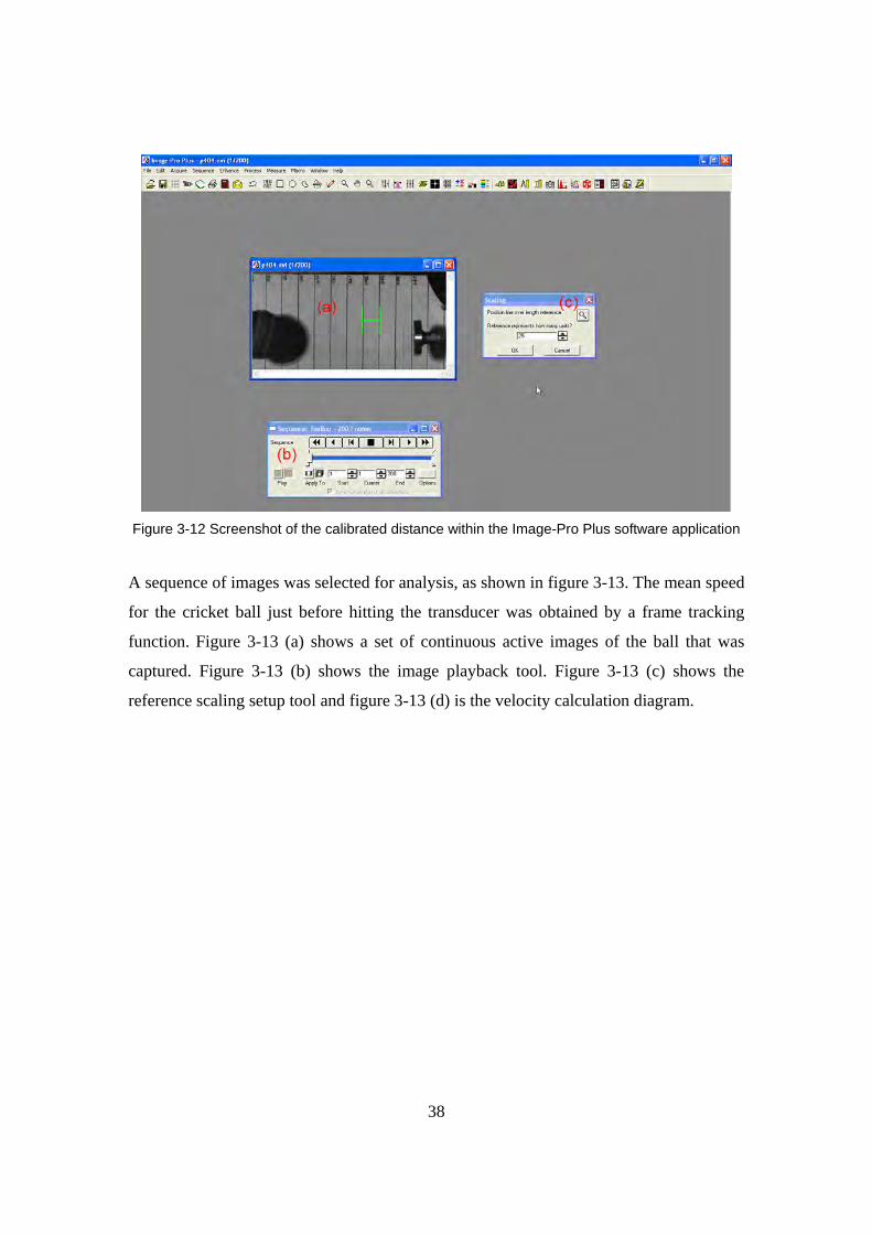
Prior to analysing the images, a reference spatial calibration was completed. The

reference calibration was used to characterize the optical system so that the captured

images can be correctly calibrated. Figure 3-12 (a) shows the green reference line

represents 25mm in physical measurements. Figure 3-12 (b) shows the image playback

tool and figure 3-12 (c) shows the reference scaling setup tool.

38

Figure 3-12 Screenshot of the calibrated distance within the Image-Pro Plus software application

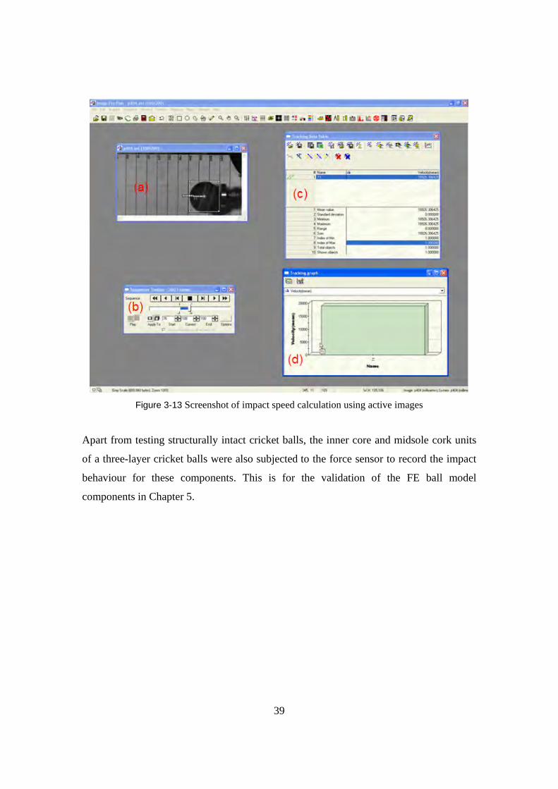
A sequence of images was selected for analysis, as shown in figure 3-13. The mean speed

for the cricket ball just before hitting the transducer was obtained by a frame tracking

function. Figure 3-13 (a) shows a set of continuous active images of the ball that was

captured. Figure 3-13 (b) shows the image playback tool. Figure 3-13 (c) shows the

reference scaling setup tool and figure 3-13 (d) is the velocity calculation diagram.

39

Figure 3-13 Screenshot of impact speed calculation using active images

Apart from testing structurally intact cricket balls, the inner core and midsole cork units

of a three-layer cricket balls were also subjected to the force sensor to record the impact

behaviour for these components. This is for the validation of the FE ball model

components in Chapter 5.

40

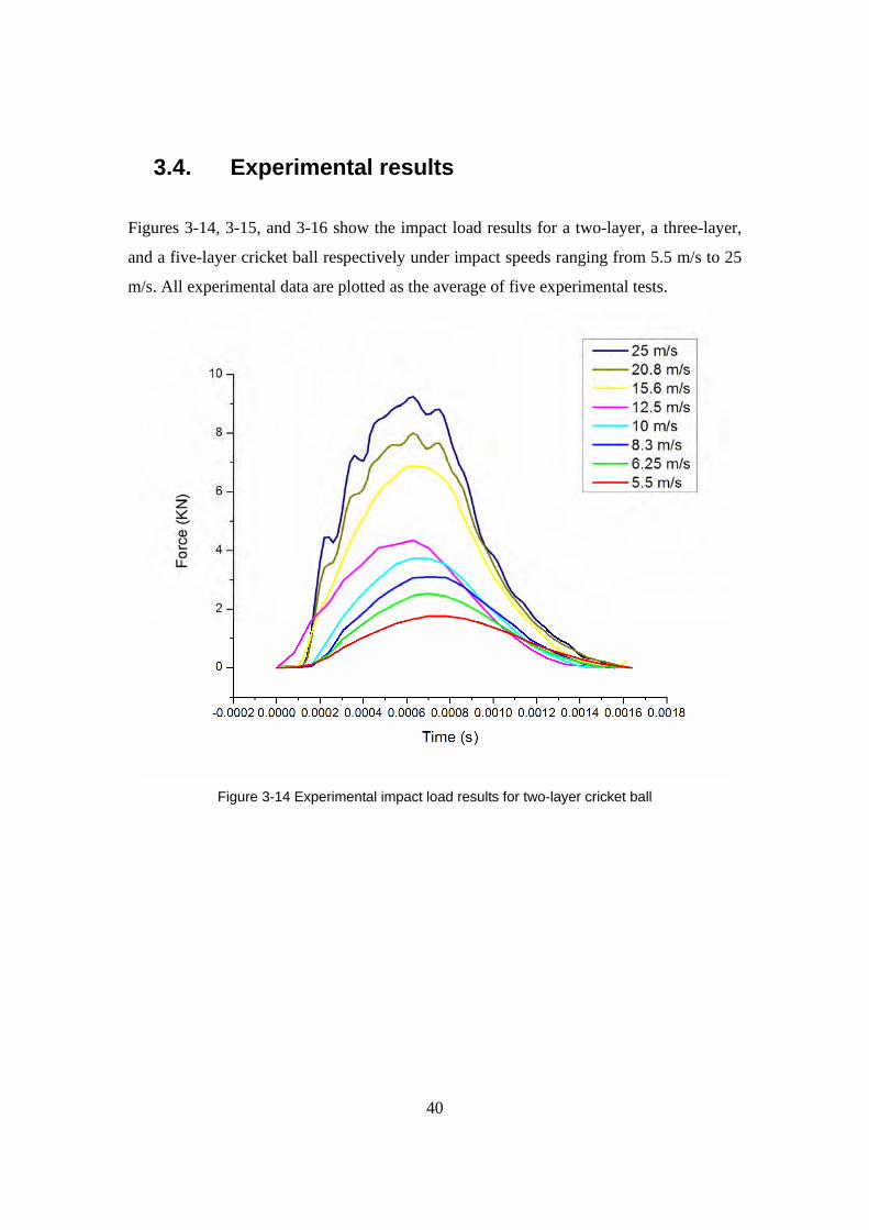
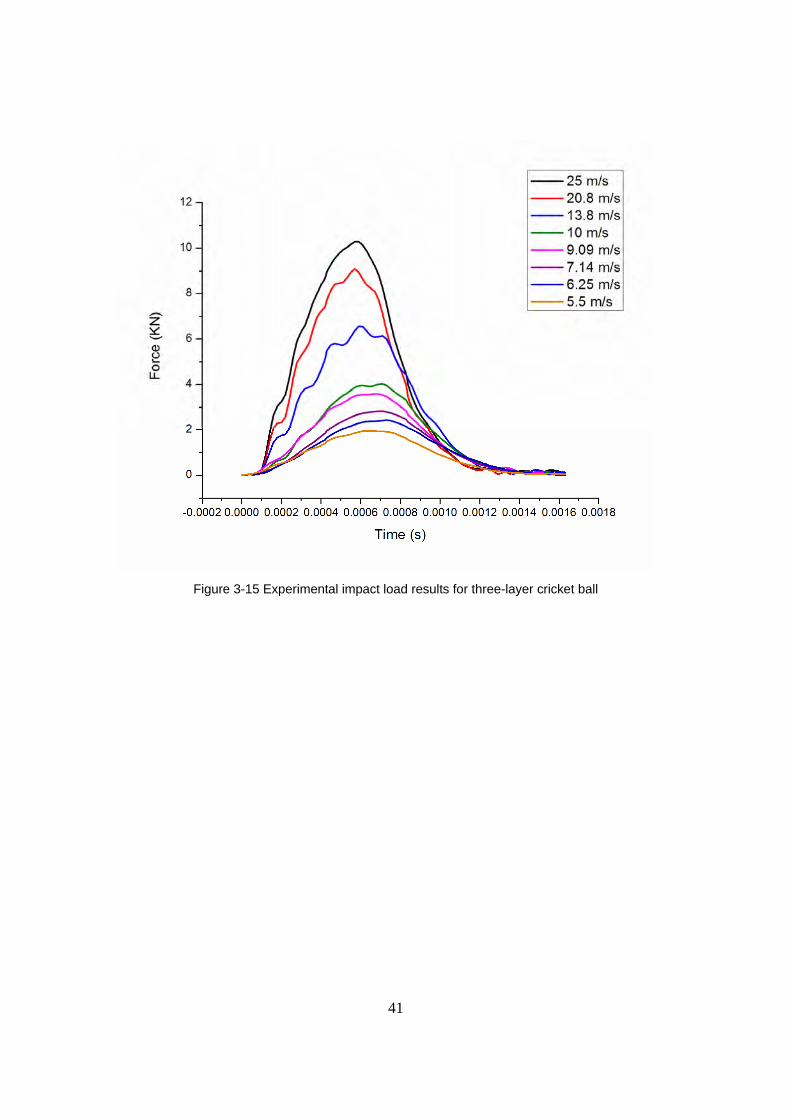
3.4. Experimental results

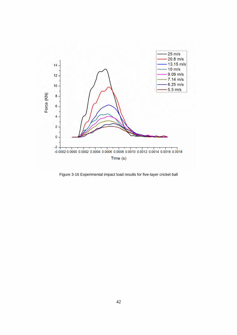
Figures 3-14, 3-15, and 3-16 show the impact load results for a two-layer, a three-layer,

and a five-layer cricket ball respectively under impact speeds ranging from 5.5 m/s to 25

m/s. All experimental data are plotted as the average of five experimental tests.

Figure 3-14 Experimental impact load results for two-layer cricket ball

41

Figure 3-15 Experimental impact load results for three-layer cricket ball

42

Figure 3-16 Experimental impact load results for five-layer cricket ball

43

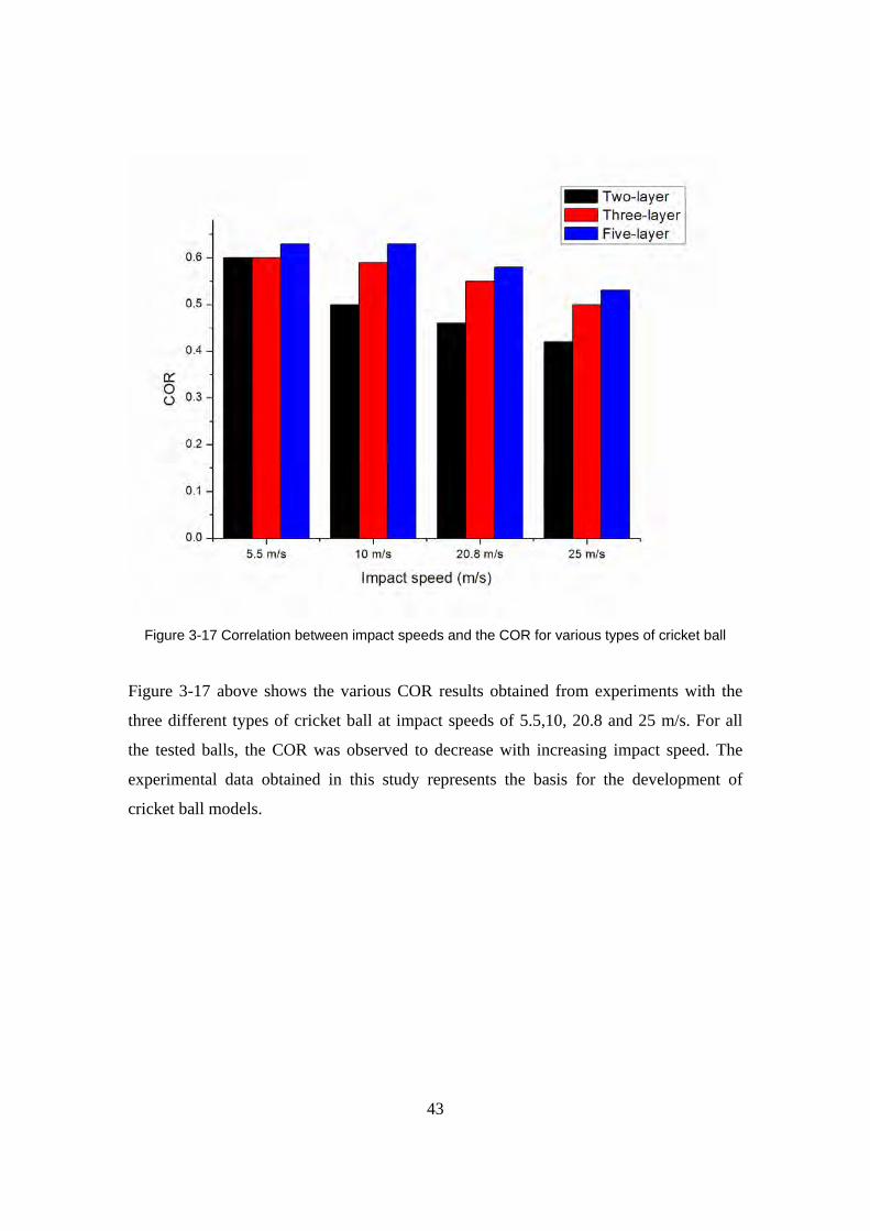
Figure 3-17 Correlation between impact speeds and the COR for various types of cricket ball

Figure 3-17 above shows the various COR results obtained from experiments with the

three different types of cricket ball at impact speeds of 5.5,10, 20.8 and 25 m/s. For all

the tested balls, the COR was observed to decrease with increasing impact speed. The

experimental data obtained in this study represents the basis for the development of

cricket ball models.

44

4. Fast-solving Mathematical Models

4.1. Introduction

In this research, two mathematical models have been developed incorporating the

experimentally determined cricket ball behaviour.

The first model termed here as “single-element model” consists of a single non-linear

spring-damper unit (figure 4-1). The second is the “three-element model” (figure 4-3),

which is a more complicated spring-damper system in which three Maxwell units are

connected in parallel. For better accuracy, the parameters of both models have been

identified as functions of impact speed.

45

4.2. The single-element non-linear model

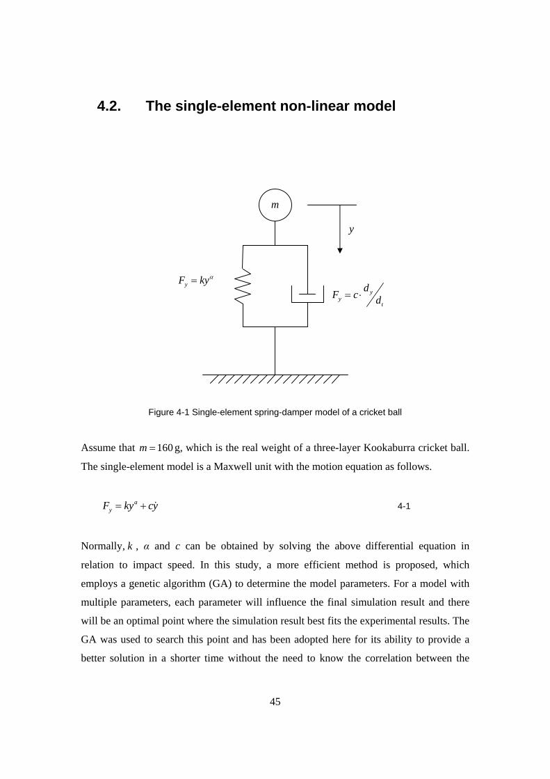
Figure 4-1 Single-element spring-damper model of a cricket ball

Assume that 160m = g, which is the real weight of a three-layer Kookaburra cricket ball.

The single-element model is a Maxwell unit with the motion equation as follows.

a

yF ky cy= + & 4-1

Normally, k , α and c can be obtained by solving the above differential equation in

relation to impact speed. In this study, a more efficient method is proposed, which

employs a genetic algorithm (GA) to determine the model parameters. For a model with

multiple parameters, each parameter will influence the final simulation result and there

will be an optimal point where the simulation result best fits the experimental results. The

GA was used to search this point and has been adopted here for its ability to provide a

better solution in a shorter time without the need to know the correlation between the

y

yF kyα= y

yt

dF c d= ⋅

m

46

search variables in a complex problem. This advantage becomes more evident when the

GA is applied to solve multi-element models which are very difficult to solve using

traditional search methods such as the gradient method.

Once the model has been formalised, the parameters can be defined through the GA

operator. The main objective in implementing this algorithm is to represent a solution to

the problem as a chromosome. This requires the estimation of six fundamental

parameters: chromosome representation, creation of the initial population, fitness

evaluation function, selection function, genetic operators, and termination criteria. The

definitions of the key parameters are listed below:

a) Chromosome representation: Each individual or chromosome is a combination of

the model parameters, k, a and c.

b) Creation of the initial population: GAs work with a set of artificial elements

called population. The initial population, which is a set of various combinations of

k, a and c, is generated randomly from a given range.

c) Fitness evaluation function: This function is used to evaluate the fitness of an

individual. The root mean square error (RMSE) that is calculated from the

simulation force wave and the experiment force wave is deemed as fitness

character. This means that the smaller the RMSE, the better the solution.

d) Selection function: The selection function uses the “roulette wheel” method.

e) Genetic operators: Two parents perform a simple single-point crossover. This

changes each of the bits of the parents based on the probability of mutation

(binary mutation). Figure 4-2 shows the workflow of the genetic algorithm

operations.

f) Termination criteria: This is the upper limit of generation numbers and is 200.

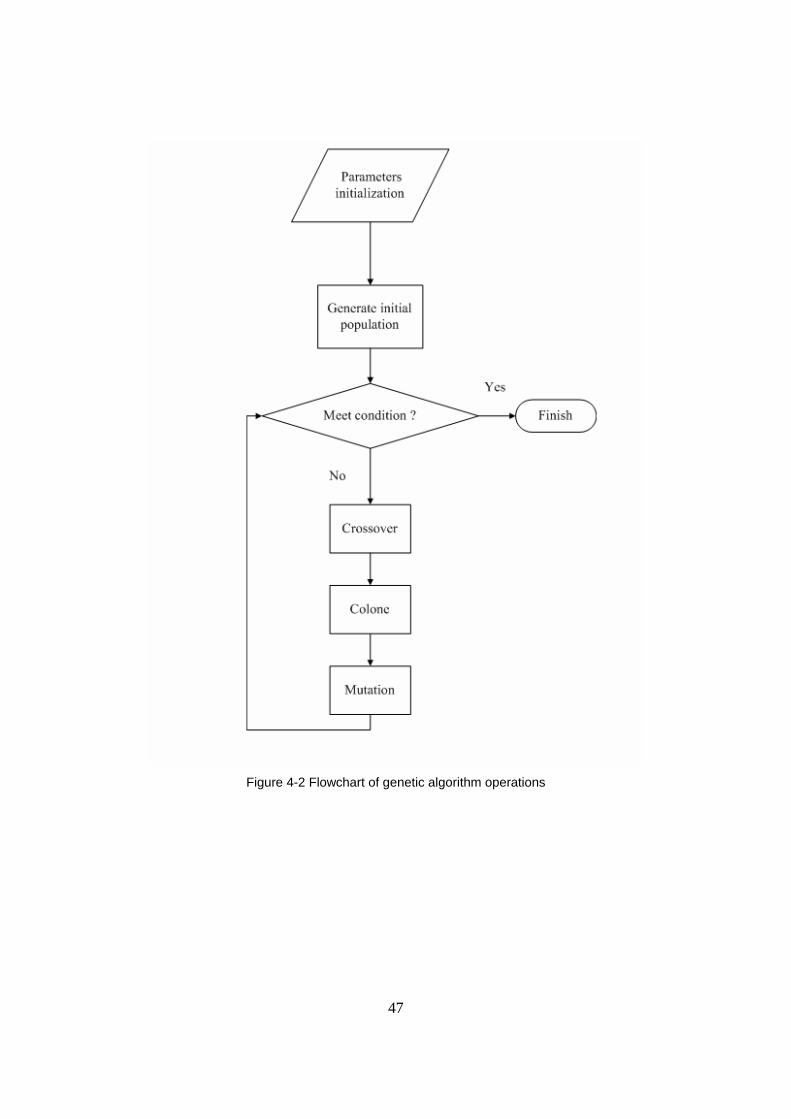
47

Figure 4-2 Flowchart of genetic algorithm operations

48

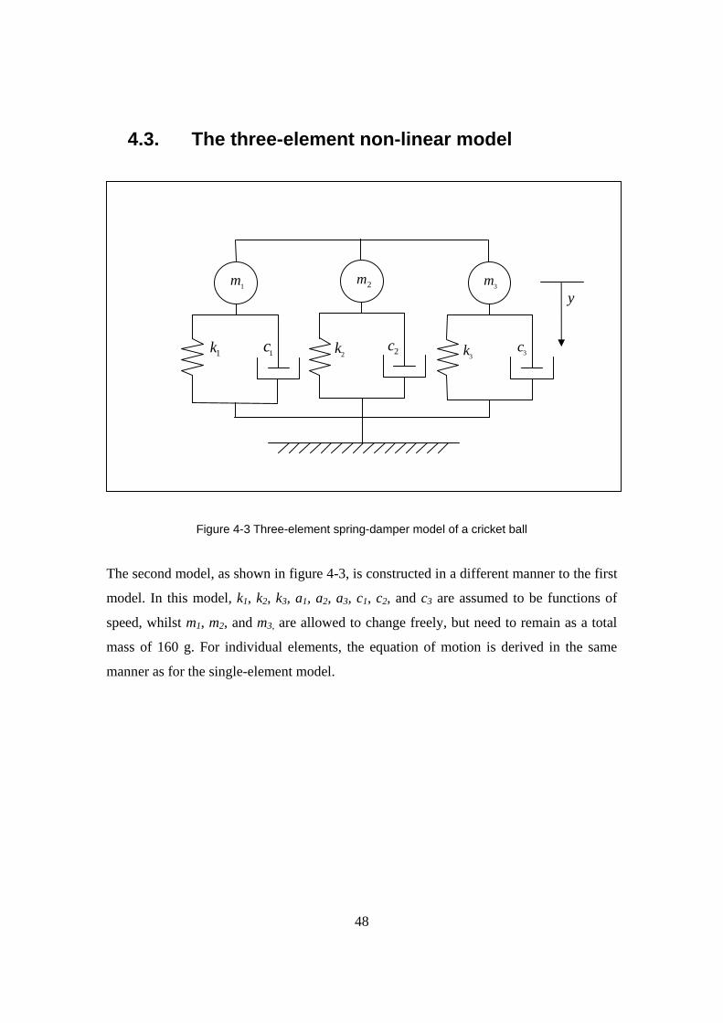
4.3. The three-element non-linear model

Figure 4-3 Three-element spring-damper model of a cricket ball

The second model, as shown in figure 4-3, is constructed in a different manner to the first

model. In this model, k1, k2, k3, a1, a2, a3, c1, c2, and c3 are assumed to be functions of

speed, whilst m1, m2, and m3, are allowed to change freely, but need to remain as a total

mass of 160 g. For individual elements, the equation of motion is derived in the same

manner as for the single-element model.

y

3k

3m

3c 2k

2m

2c

1m

1k 1c

49

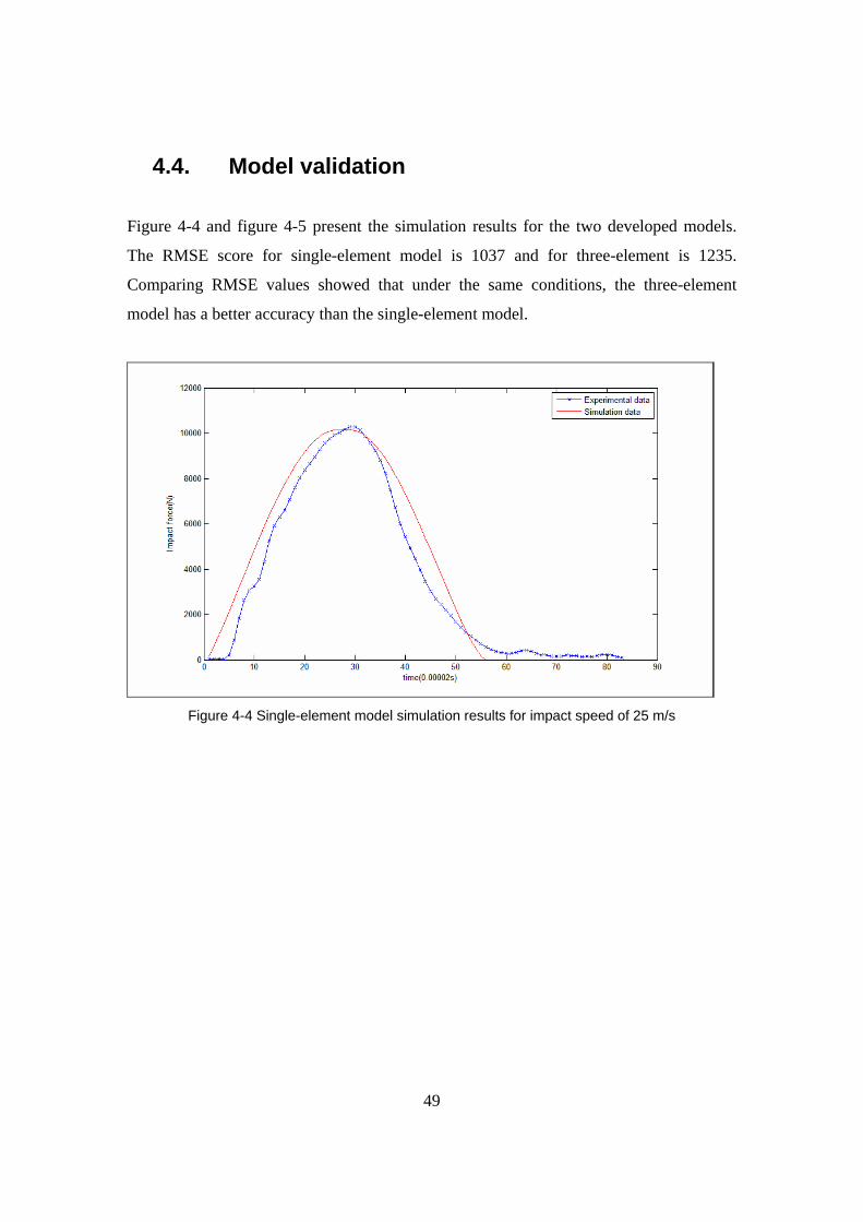
4.4. Model validation

Figure 4-4 and figure 4-5 present the simulation results for the two developed models.

The RMSE score for single-element model is 1037 and for three-element is 1235.

Comparing RMSE values showed that under the same conditions, the three-element

model has a better accuracy than the single-element model.

Figure 4-4 Single-element model simulation results for impact speed of 25 m/s

50

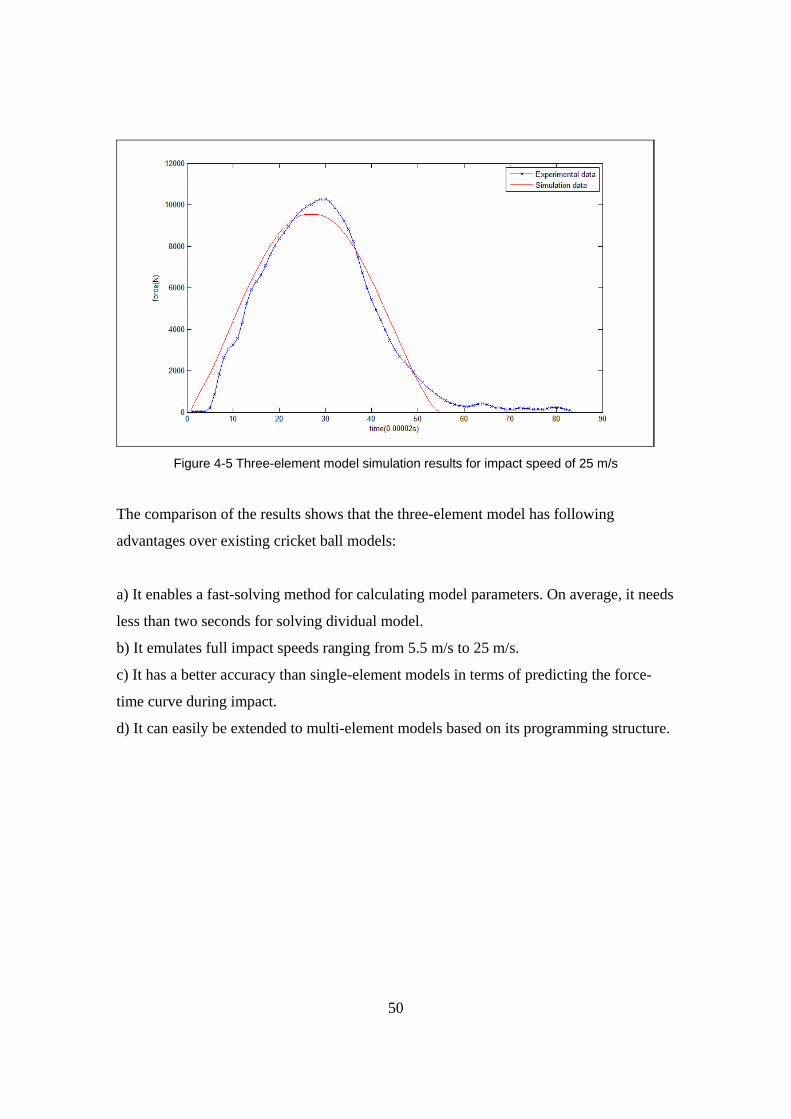
Figure 4-5 Three-element model simulation results for impact speed of 25 m/s

The comparison of the results shows that the three-element model has following

advantages over existing cricket ball models:

a) It enables a fast-solving method for calculating model parameters. On average, it needs

less than two seconds for solving dividual model.

b) It emulates full impact speeds ranging from 5.5 m/s to 25 m/s.

c) It has a better accuracy than single-element models in terms of predicting the force-

time curve during impact.

d) It can easily be extended to multi-element models based on its programming structure.

51

5. Detailed Finite Element Model

5.1. Introduction

The development of numerical simulations using advanced finite element (FE) models

has become a subject of increasing interest in the field of sports research. FE models can

provide more accurate simulations than other conventional mathematical models. They

can provide understanding of impact mechanisms in complex systems—such as stress

propagation waves and energy transactions.

This chapter presents the development of a validated, multi-layered and multi-material

FE model of a cricket ball. The developed FE model includes detailed ball geometry and

verified material parameters. It can also simulate a wide range of impact speeds. The

development of the FE model includes the construction of geometry, the assignment of

material properties, and the application of surface interactions between the different

components of the ball. During the simulation, temperature effect was not considered.

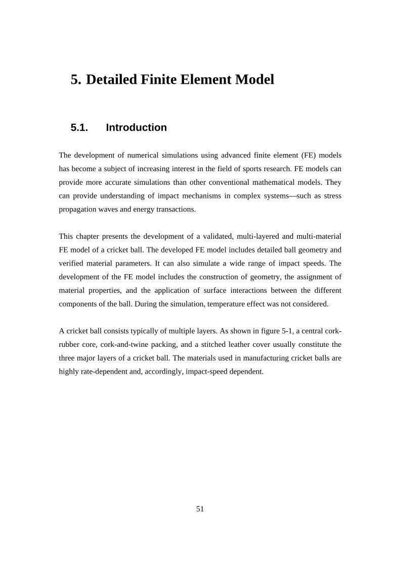
A cricket ball consists typically of multiple layers. As shown in figure 5-1, a central cork-

rubber core, cork-and-twine packing, and a stitched leather cover usually constitute the

three major layers of a cricket ball. The materials used in manufacturing cricket balls are

highly rate-dependent and, accordingly, impact-speed dependent.

52

Figure 5-1 Cross-section of a three-layer cricket ball

Table 5-1 presents the detailed specifications of the three layers that were measured from

a real Kookaburra cricket ball.

Layer Mass

( g )

Diameter

( mm )

Volume

( 3mm )

ρ

( 3/T mm )

Inner core 29 40 33510 8.65×10–10

Midsole cork layer 61 62 91278 6.68×10–10

Leather cover 80 72 70644 11.32×10–10

Table 5-1 Three-layer cricket ball specifications

53

5.2. Development of the FE model

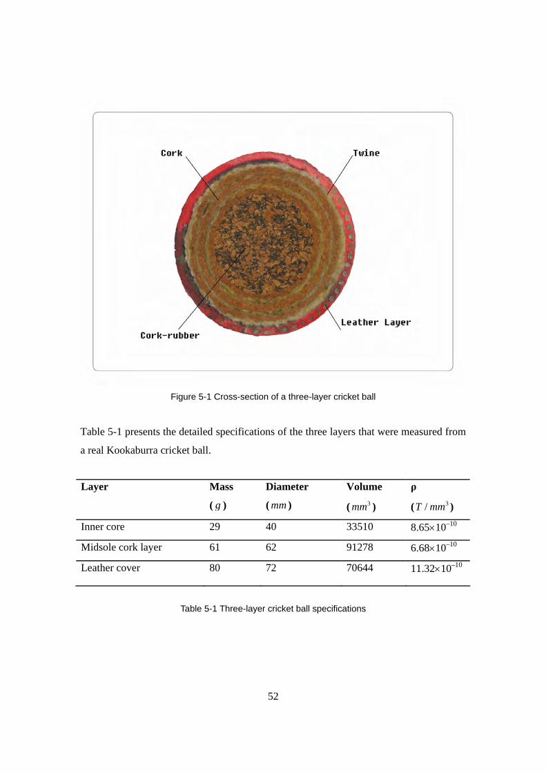
The FE model presented here consists of three major components (figure 5-2): a central

solid sphere, a middle hollow sphere and an external hollow sphere. These components

are respectively developed to emulate the cork-rubber inner core, cork-and-twine midsole

layer, and the leather cover of the cricket ball.

Figure 5-2 Detailed FE model components

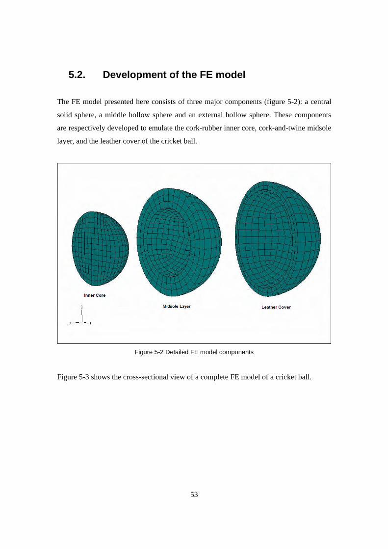
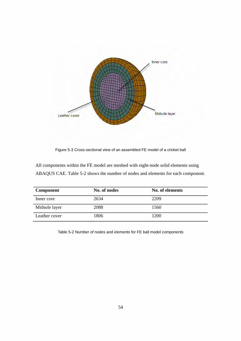
Figure 5-3 shows the cross-sectional view of a complete FE model of a cricket ball.

54

Figure 5-3 Cross-sectional view of an assembled FE model of a cricket ball

All components within the FE model are meshed with eight-node solid elements using

ABAQUS CAE. Table 5-2 shows the number of nodes and elements for each component.

Component No. of nodes No. of elements

Inner core 2634 2209

Midsole layer 2088 1560

Leather cover 1806 1200

Table 5-2 Number of nodes and elements for FE ball model components

55

In non-linear dynamic Finite Element Analysis, there are basically two numerical

integration methods; the implicit method and the explicit method. Both methods are

incremental, i.e. the analysis is divided into many small increments. The final solution

is obtained from the progress through the incremental responses. In the implicit

method, dynamic equilibrium has to be achieved at the end of each increment using

iteration techniques. On the other hand, the explicit method achieves a solution by

explicitly advancing the kinematic state from the previous increment. The size of the

time increment needs to be very small in order to avoid numerical instability. The size

of the time increment depends on the mesh density and the highest natural frequency

of the model. Therefore, a very large number of increments is needed for the analysis.

However, the computational cost per increment using the explicit method is much

smaller than that of the implicit method. The small size of the time increments makes

the explicit method more suitable for non-linear dynamic analysis occurring over a

very short period of time, such as impact analysis. Therefore, the dynamic explicit

method of analysis has been used throughout this study to simulate the impact of the

cricket ball to other surfaces.

In this study, finite element analysis was performed using the commercially available

non-linear FEM program, ABAQUS/Explicit, Version 6.6, which was run in

Microsoft Windows XP on a high-performance personal computer.

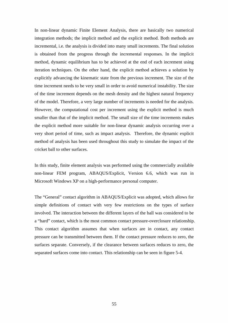
The “General” contact algorithm in ABAQUS/Explicit was adopted, which allows for

simple definitions of contact with very few restrictions on the types of surface

involved. The interaction between the different layers of the ball was considered to be

a “hard” contact, which is the most common contact pressure-overclosure relationship.

This contact algorithm assumes that when surfaces are in contact, any contact

pressure can be transmitted between them. If the contact pressure reduces to zero, the

surfaces separate. Conversely, if the clearance between surfaces reduces to zero, the

separated surfaces come into contact. This relationship can be seen in figure 5-4.

56

Figure 5-4 Pressure-overclosure relationship of “hard” contact in ABAQUS

The contact force between the cricket ball and the rigid surface was calculated by

adopting the “penalty method”. Once the initial basic FE model was developed, it was

then essential to choose the correct material models and corresponding associated

parameters.

The detailed FE model was developed through a three-step process. First, an inner

core unit was modelled separately and calibrated against experimental tests. Then, a

midsole layer model was added onto the verified core unit. Finally, after the midsole

unit was verified against experimental tests, a leather cover model was incorporated to

produce a complete cricket ball model.

The following sections describe how each component was modelled and verified

against experimental results and how those model parameters were determined.

No pressure when

no contact

Clearance

Contact pressure Any pressure possible when

in contact

57

5.2.1. The inner core

The inner core of a cricket ball is generally a rubber-like material although consisting

of mixed rubber and cork. The non-linear elastic properties of this inner core were

represented by a hyperelastic material model, as theoretically developed below.

Therefore, it was assumed that the inner core material is isotropic and incompressible.

Rubber and rubber-like material properties are not represented by Hooke’s law, but

are characterized by a strain-energy function. The relationship between the strain-

energy function and stress is

EUT∂∂

= , ijij

UTe

∂=∂

5-1

where T is the 2nd Piola-Kirchhoff stress tensor , E is the Green-Lagrange strain

tensor and U is the strain-energy function. Following this, the Cauchy stress,σ, is

obtained from

1 TFTFJ

σ = 5-2

where J = Fdet is the Jacobian determinant of F , and F is the deformation gradient

tensor given by

XxF

∂∂

= , j

iij X

xF

∂∂

= 5-3

Where ix represents the current configuration and jX represents the reference

configuration. The strain-energy function, U, is a function of the principal invariants,

21, II and 3I :

1 ( )I trace B= 5-4

58

2 22 1

1 ( ( ))2

I I trace B= − 5-5

and

3 det( )I B= 5-6

Where TB FF= is the left Cauchy-Green deformation tensor. For incompressible

material,

1=J , 1, 2( )U U I I= 5-7

Then, the general form for the constitutive model of hyperelasticity is given by

21

1 2 2

2 U U UpI I B BI I I

σ⎡ ⎤⎛ ⎞∂ ∂ ∂

= − + + −⎢ ⎥⎜ ⎟∂ ∂ ∂⎝ ⎠⎣ ⎦ 5-8

Where p is the hydrostatic pressure arising from the incompressibility constraint.

There are several hyperelastic material models that are commonly used to describe

rubber and other elastomeric materials on the basis of strain energy potential. The

Mooney-Rivlin model is chosen for this study and its constitution equation can be

expressed as

( ) ( ) ( )2

10 1 01 21

13 3 1elU C I C I JD

= − + − + − 5-9

Where U is the strain energy per unit of reference volume; C10, C01 and D1 are

temperature-dependent material parameters; and 1I and 2I are the first and second

deviatoric strain invariants. Jel is the elastic volume ratio.

In order to define material parameters, uniaxial compression tests were conducted

using the INSTRON universal testing machine. These compression tests were

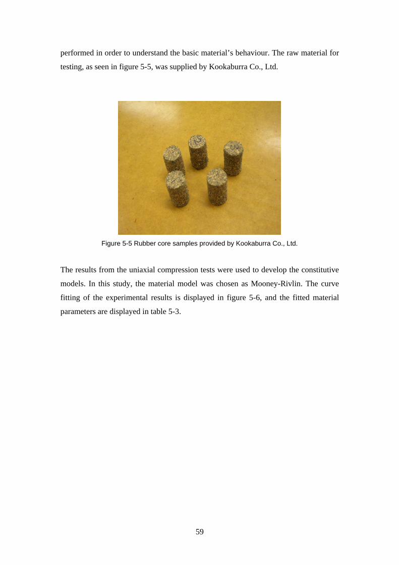
59

performed in order to understand the basic material’s behaviour. The raw material for

testing, as seen in figure 5-5, was supplied by Kookaburra Co., Ltd.

Figure 5-5 Rubber core samples provided by Kookaburra Co., Ltd.

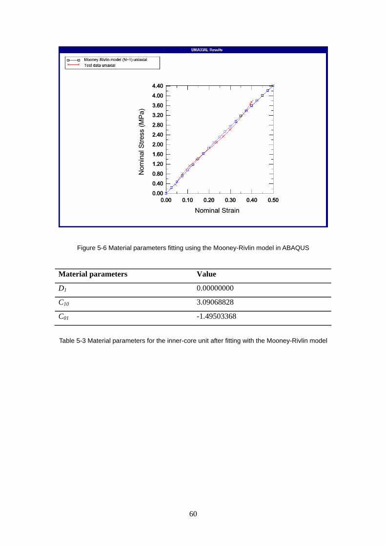
The results from the uniaxial compression tests were used to develop the constitutive

models. In this study, the material model was chosen as Mooney-Rivlin. The curve

fitting of the experimental results is displayed in figure 5-6, and the fitted material

parameters are displayed in table 5-3.

60

Figure 5-6 Material parameters fitting using the Mooney-Rivlin model in ABAQUS

Material parameters Value

D1 0.00000000

C10 3.09068828

C01 -1.49503368

Table 5-3 Material parameters for the inner-core unit after fitting with the Mooney-Rivlin model

61

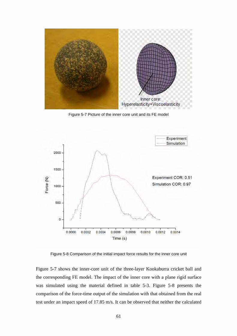
Figure 5-7 Picture of the inner core unit and its FE model

Figure 5-8 Comparison of the initial impact force results for the inner core unit

Figure 5-7 shows the inner-core unit of the three-layer Kookaburra cricket ball and

the corresponding FE model. The impact of the inner core with a plane rigid surface

was simulated using the material defined in table 5-3. Figure 5-8 presents the

comparison of the force-time output of the simulation with that obtained from the real

test under an impact speed of 17.85 m/s. It can be observed that neither the calculated

62

peak force nor the contact time agrees with the experimental results. This is generally

because the material properties have been derived from a quasi-static test. A dynamic

impact test involves large local deformation and rapid strain changes. Therefore, the

ideal material test would be an instantaneous recording of stress/strain response

during impact. Moreover, there is no energy loss being considered during this basic

simulation, which also results in the calculated COR being higher than the

experimentally measured value. Although the initial static response of the material

was linear, introducing such a response in the model produced large discrepancy with

the experimental results. This response was modified through the optimization

process into non-linear behaviour, which produced agreement between numerical

results and experimental measurements.

Due to physical limitations, it was impossible to measure the material properties at

high impact velocities. An alternative robust approach as detailed below was applied

in order to indirectly determine the material properties. The material parameters under

dynamic conditions were determined by modifying the initial material properties,

obtained from the quasi-static test, to satisfy the results of experimental impact test of

the inner core at different impact speeds.

The entire process is based on a reverse engineering technique using

modeFRONTIER 3.2 (ESTECO Inc., Italy), a computer program used for process

integration and optimization (figure 5-9) which integrated ABAQUS and MATLAB

to include FE simulation, results extraction, evaluation, and optimization.

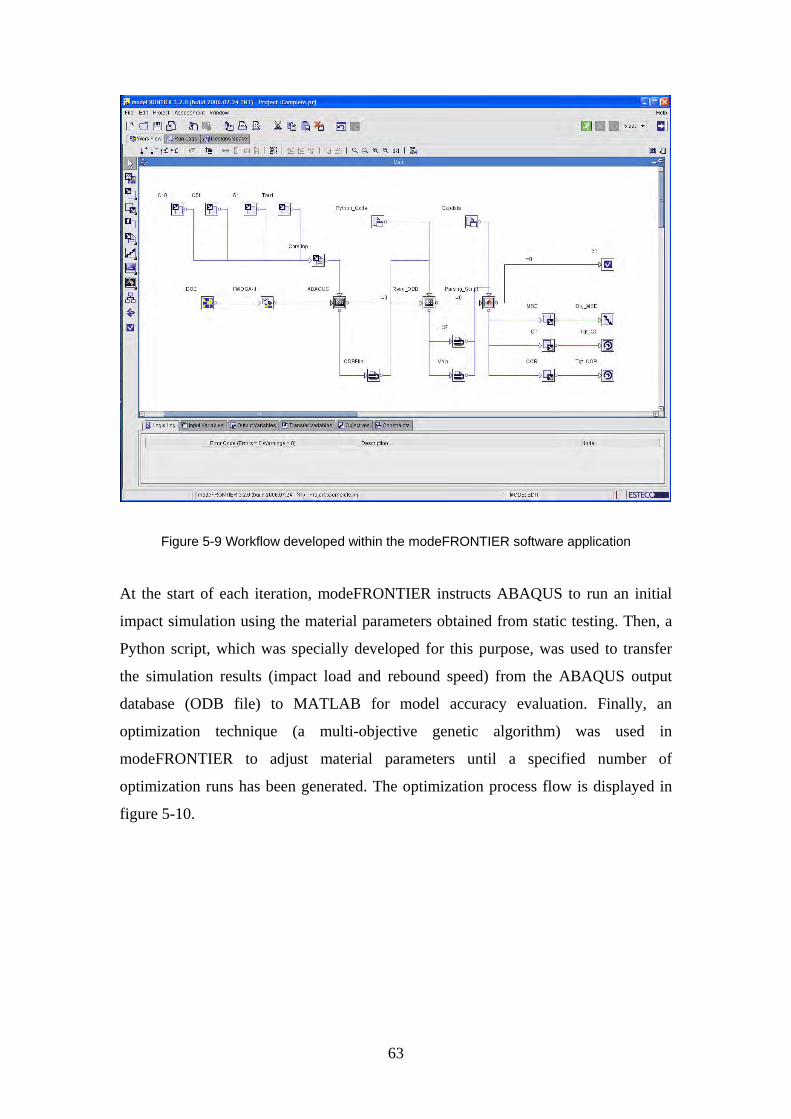
63

Figure 5-9 Workflow developed within the modeFRONTIER software application

At the start of each iteration, modeFRONTIER instructs ABAQUS to run an initial

impact simulation using the material parameters obtained from static testing. Then, a

Python script, which was specially developed for this purpose, was used to transfer

the simulation results (impact load and rebound speed) from the ABAQUS output

database (ODB file) to MATLAB for model accuracy evaluation. Finally, an

optimization technique (a multi-objective genetic algorithm) was used in

modeFRONTIER to adjust material parameters until a specified number of

optimization runs has been generated. The optimization process flow is displayed in

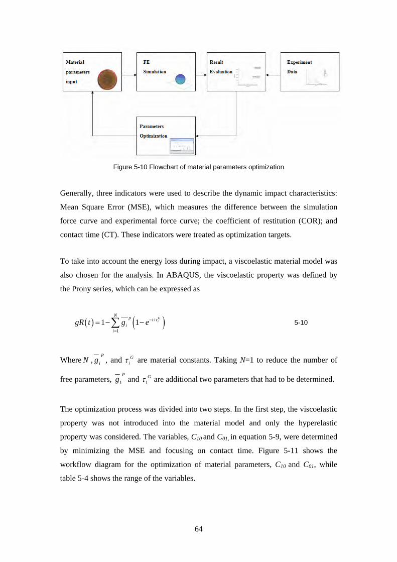
figure 5-10.

64

Figure 5-10 Flowchart of material parameters optimization

Generally, three indicators were used to describe the dynamic impact characteristics:

Mean Square Error (MSE), which measures the difference between the simulation

force curve and experimental force curve; the coefficient of restitution (COR); and

contact time (CT). These indicators were treated as optimization targets.

To take into account the energy loss during impact, a viscoelastic material model was

also chosen for the analysis. In ABAQUS, the viscoelastic property was defined by

the Prony series, which can be expressed as

( ) ( )/

11 1

Gi

N p ti

igR t g e τ−

=

= − −∑ 5-10

Where N ,P

ig , and Giτ are material constants. Taking N=1 to reduce the number of

free parameters, 1

Pg and 1

Gτ are additional two parameters that had to be determined.

The optimization process was divided into two steps. In the first step, the viscoelastic

property was not introduced into the material model and only the hyperelastic

property was considered. The variables, C10 and C01, in equation 5-9, were determined

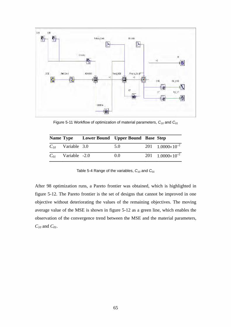
by minimizing the MSE and focusing on contact time. Figure 5-11 shows the

workflow diagram for the optimization of material parameters, C10 and C01, while

table 5-4 shows the range of the variables.

65

Figure 5-11 Workflow of optimization of material parameters, C10 and C01

Name Type Lower Bound Upper Bound Base Step

C10 Variable 3.0 5.0 201 1.0000×10–2

C01 Variable -2.0 0.0 201 1.0000×10–2

Table 5-4 Range of the variables, C10 and C01

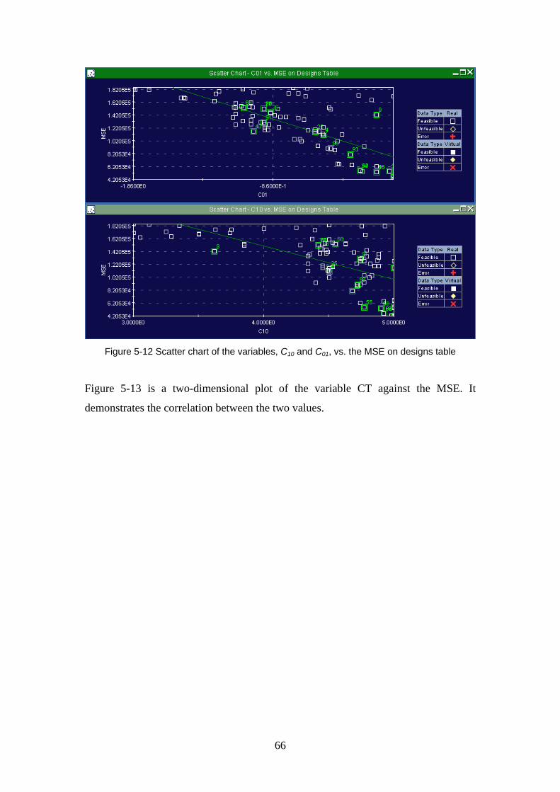
After 98 optimization runs, a Pareto frontier was obtained, which is highlighted in

figure 5-12. The Pareto frontier is the set of designs that cannot be improved in one

objective without deteriorating the values of the remaining objectives. The moving

average value of the MSE is shown in figure 5-12 as a green line, which enables the

observation of the convergence trend between the MSE and the material parameters,

C10 and C01.

66

Figure 5-12 Scatter chart of the variables, C10 and C01, vs. the MSE on designs table

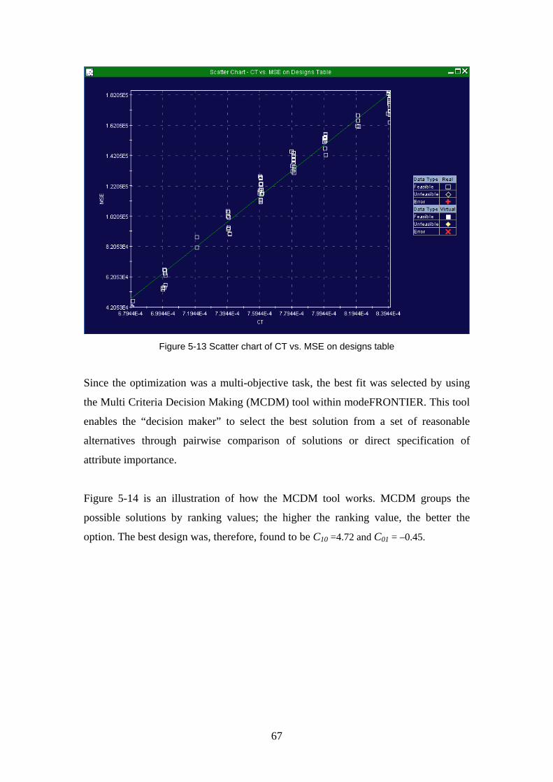
Figure 5-13 is a two-dimensional plot of the variable CT against the MSE. It

demonstrates the correlation between the two values.

67

Figure 5-13 Scatter chart of CT vs. MSE on designs table

Since the optimization was a multi-objective task, the best fit was selected by using

the Multi Criteria Decision Making (MCDM) tool within modeFRONTIER. This tool

enables the “decision maker” to select the best solution from a set of reasonable

alternatives through pairwise comparison of solutions or direct specification of

attribute importance.

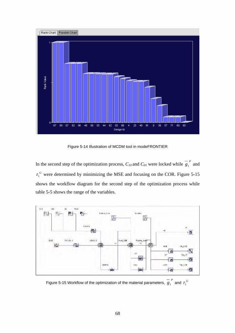
Figure 5-14 is an illustration of how the MCDM tool works. MCDM groups the

possible solutions by ranking values; the higher the ranking value, the better the

option. The best design was, therefore, found to be C10 =4.72 and C01 = –0.45.

68

Figure 5-14 Illustration of MCDM tool in modeFRONTIER

In the second step of the optimization process, C10 and C01 were locked while 1

Pg and

1Gτ were determined by minimizing the MSE and focusing on the COR. Figure 5-15

shows the workflow diagram for the second step of the optimization process while

table 5-5 shows the range of the variables.

Figure 5-15 Workflow of the optimization of the material parameters, 1

Pg and 1

Gτ

69

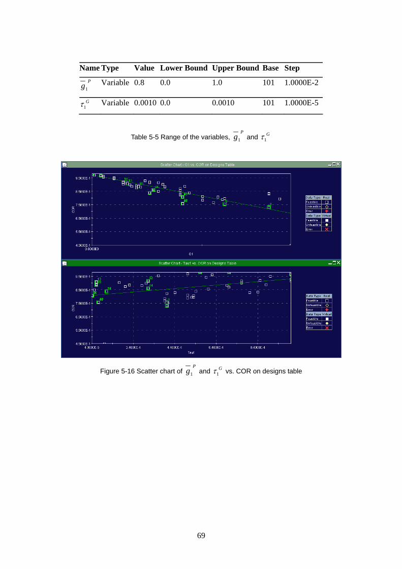
Name Type Value Lower Bound Upper Bound Base Step

1

Pg Variable 0.8 0.0 1.0 101 1.0000E-2

1Gτ Variable 0.0010 0.0 0.0010 101 1.0000E-5

Table 5-5 Range of the variables, 1

Pg and 1

Gτ

Figure 5-16 Scatter chart of 1

Pg and 1

Gτ vs. COR on designs table

70

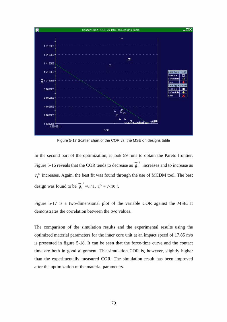
Figure 5-17 Scatter chart of the COR vs. the MSE on designs table

In the second part of the optimization, it took 59 runs to obtain the Pareto frontier.

Figure 5-16 reveals that the COR tends to decrease as 1

Pg increases and to increase as

1Gτ increases. Again, the best fit was found through the use of MCDM tool. The best

design was found to be 1

Pg =0.41, 1

Gτ = 7×10–5.

Figure 5-17 is a two-dimensional plot of the variable COR against the MSE. It

demonstrates the correlation between the two values.

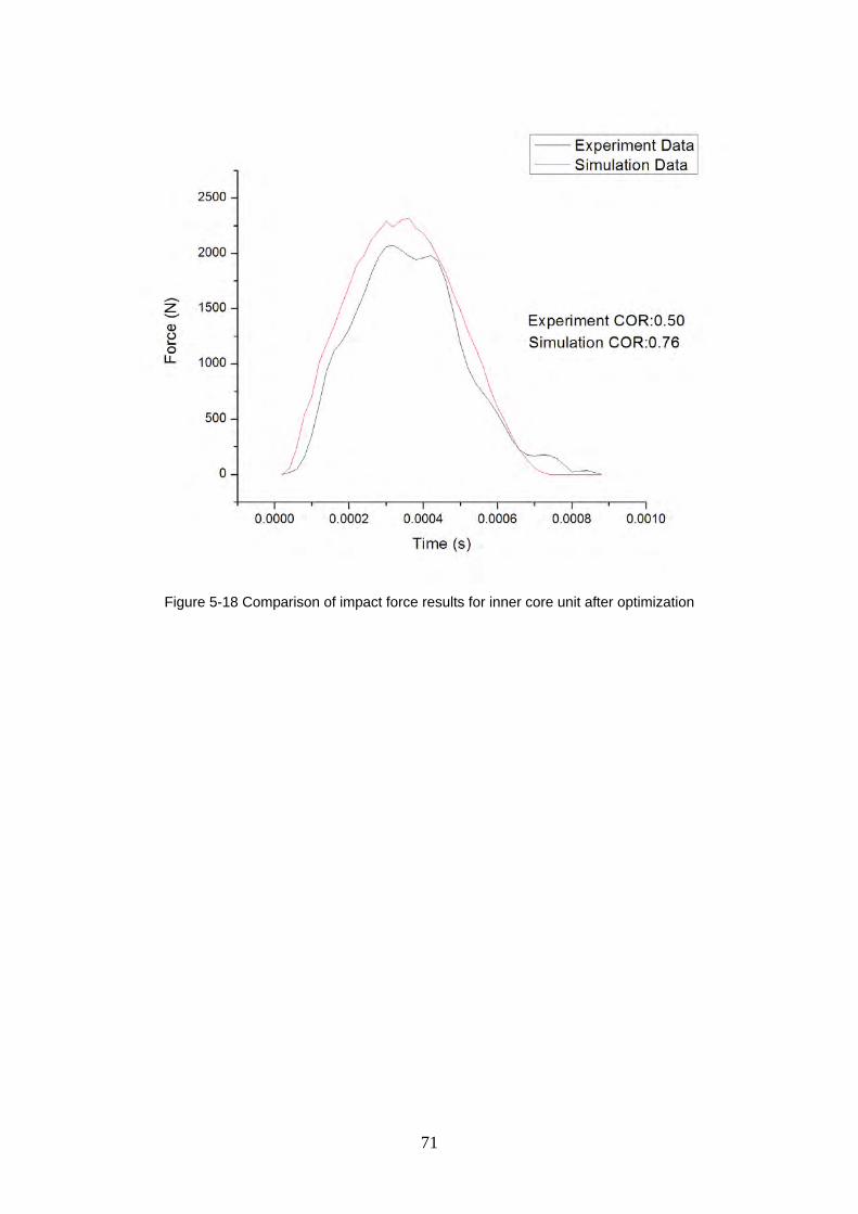
The comparison of the simulation results and the experimental results using the

optimized material parameters for the inner core unit at an impact speed of 17.85 m/s

is presented in figure 5-18. It can be seen that the force-time curve and the contact

time are both in good alignment. The simulation COR is, however, slightly higher

than the experimentally measured COR. The simulation result has been improved

after the optimization of the material parameters.

71

Figure 5-18 Comparison of impact force results for inner core unit after optimization

72

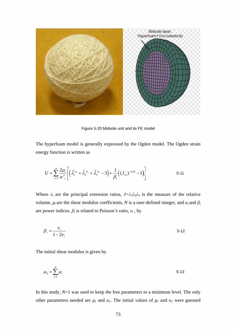
5.2.2. The midsole layer

The midsole cork layer is a composite structure made of cellular thin cork shells

wound with yarn. Figure 5-19 shows the raw material used to manufacture the

midsole cork layer. As the midsole cork layer is the main part of the cricket ball, it

will be treated as a homogeneous continuum of hyperfoam. The FE model of the

midsole unit is a hollow shell unit that emulates the midsole layer containing the inner

core (figure 5-20).

Figure 5-19 Sample of cork and yarn layer material provided by Kookaburra Co., Ltd.

73

Figure 5-20 Midsole unit and its FE model

The hyperfoam model is generally expressed by the Ogden model. The Ogden strain

energy function is written as

( ) ( )1 2 321

2 1ˆ ˆ ˆ 3 ( ) 1i i i i i

Ni

eli i i

U Jα α α α βµ λ λ λα β

−

=

⎡ ⎤= + + − + −⎢ ⎥

⎣ ⎦∑

5-11

Where λi are the principal extension ratios, J=λ1λ2λ3 is the measure of the relative

volume, µi are the shear modulus coefficients, N is a user-defined integer, and αi and βi

are power indices. βi is related to Poisson’s ratio, vi , by

iβi

i

vv21−

= 5-12

The initial shear modulus is given by

0

1

N

ii

µ µ=

=∑ 5-13

In this study, N=1 was used to keep the free parameters to a minimum level. The only

other parameters needed are µ1 and α1. The initial values of µ1 and α1 were guessed

74

and improved during the optimization process. To account for the material time

dependence during impact, the viscoelastic property of the material was included in

the model as well. The material parameters were determined by fitting the simulation

results to the experimental results using the same approach as explained in section

5.2.1. After numerical treatment, the parameters were found to be µ1=70.3, α1=4.0,

1

Pg =0, and 1

Gτ =0.00041.

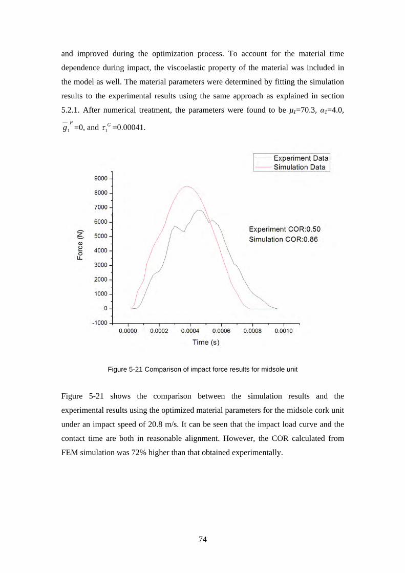
Figure 5-21 Comparison of impact force results for midsole unit

Figure 5-21 shows the comparison between the simulation results and the

experimental results using the optimized material parameters for the midsole cork unit

under an impact speed of 20.8 m/s. It can be seen that the impact load curve and the

contact time are both in reasonable alignment. However, the COR calculated from

FEM simulation was 72% higher than that obtained experimentally.

75

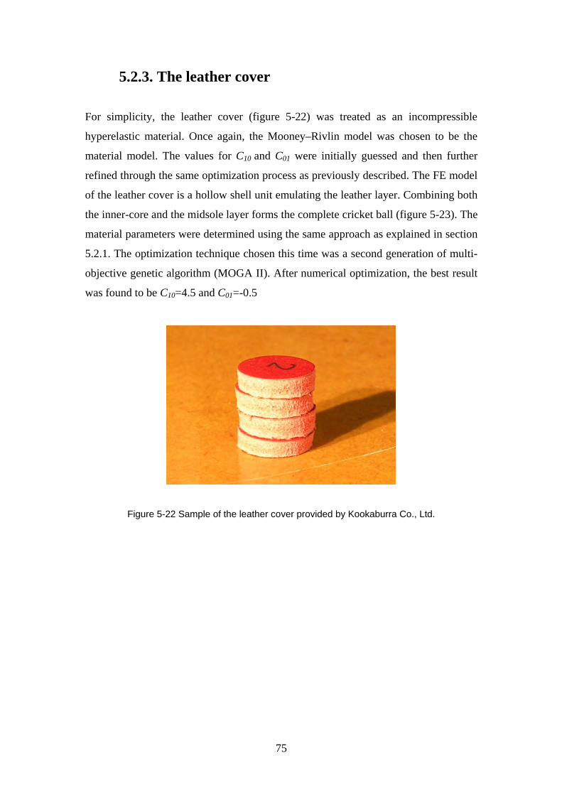
5.2.3. The leather cover

For simplicity, the leather cover (figure 5-22) was treated as an incompressible

hyperelastic material. Once again, the Mooney–Rivlin model was chosen to be the

material model. The values for C10 and C01 were initially guessed and then further

refined through the same optimization process as previously described. The FE model

of the leather cover is a hollow shell unit emulating the leather layer. Combining both

the inner-core and the midsole layer forms the complete cricket ball (figure 5-23). The

material parameters were determined using the same approach as explained in section

5.2.1. The optimization technique chosen this time was a second generation of multi-

objective genetic algorithm (MOGA II). After numerical optimization, the best result

was found to be C10=4.5 and C01=-0.5

Figure 5-22 Sample of the leather cover provided by Kookaburra Co., Ltd.

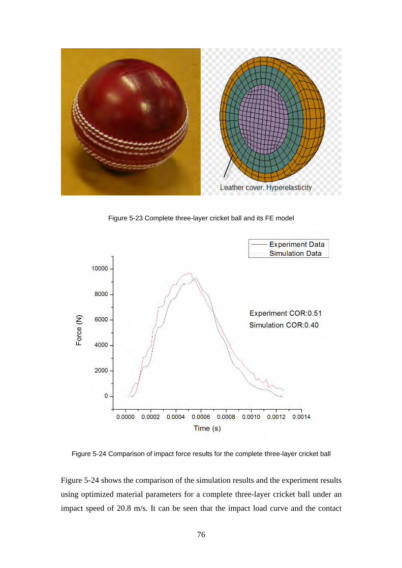
76

Figure 5-23 Complete three-layer cricket ball and its FE model

Figure 5-24 Comparison of impact force results for the complete three-layer cricket ball

Figure 5-24 shows the comparison of the simulation results and the experiment results

using optimized material parameters for a complete three-layer cricket ball under an

impact speed of 20.8 m/s. It can be seen that the impact load curve and the contact

77

time are both in good alignment. However, the COR calculated from FEM simulation

was 21% lower than that obtained experimentally.

5.2.4. Oblique impact

In the real game, the cricket ball generally lands obliquely on an object. An initial

attempt was made to extend the normal impact model to one that could be used for

oblique impacts. This was achieved by incorporating a hypothetical parameter

representing the coefficient of friction between the ball and the surface. In addition,

the friction coefficient was assumed to remain constant during impact. The cricket

ball was also assumed to approach the surface without spin. An oblique impact at an

angle of 34o was simulated at a ball velocity of 37 m/s. Figure 5-25 shows the

animation of oblique impact and rebound of the cricket ball.

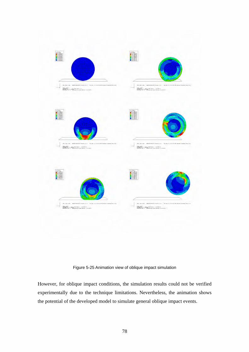
78

Figure 5-25 Animation view of oblique impact simulation

However, for oblique impact conditions, the simulation results could not be verified

experimentally due to the technique limitations. Nevertheless, the animation shows

the potential of the developed model to simulate general oblique impact events.

79

6. The Universal Structural Model

6.1. Introduction

In any FE analysis involving a cricket ball, a significant effort is spent on modelling

the ball. Creating a detailed and complex model would enhance the understanding of

the behaviour of its complex structure, but it would also generate a large number of

elements, which would increase model size, analysis time and the amount of

computing resources needed for the analysis. Therefore, creating a simple but

accurate universal cricket ball model that can be used for the virtual design of cricket

equipment and protective gear would be beneficial.

The literature review revealed that considerable work has been done to identify

material parameters, especially when those parameters are difficult to measure

experimentally. Many researchers have evaluated these material parameters using

trial-and-error (Ujihashi et al., 2002;Smith et al., 2000). This approach often uses

measured gradients to test and then to adjust the parameters manually. Although this

approach occasionally produces good results, it represents a tedious process.

In this study, a universal FE model was created by means of predicting model

parameters. As is commonly known, calibration of non-linear FE models is a difficult

and time-consuming process as the analysis procedure is incremental and iterative. To

expedite the calibration process, an approximate FE model was developed using an

Artificial Neural Network (ANN). Such an approximate model can be seen as a

combination of an FE model template and a material parameter selection tool that is

based on the ANN model. The relationship between these models can be seen in

figure 6-1.

80

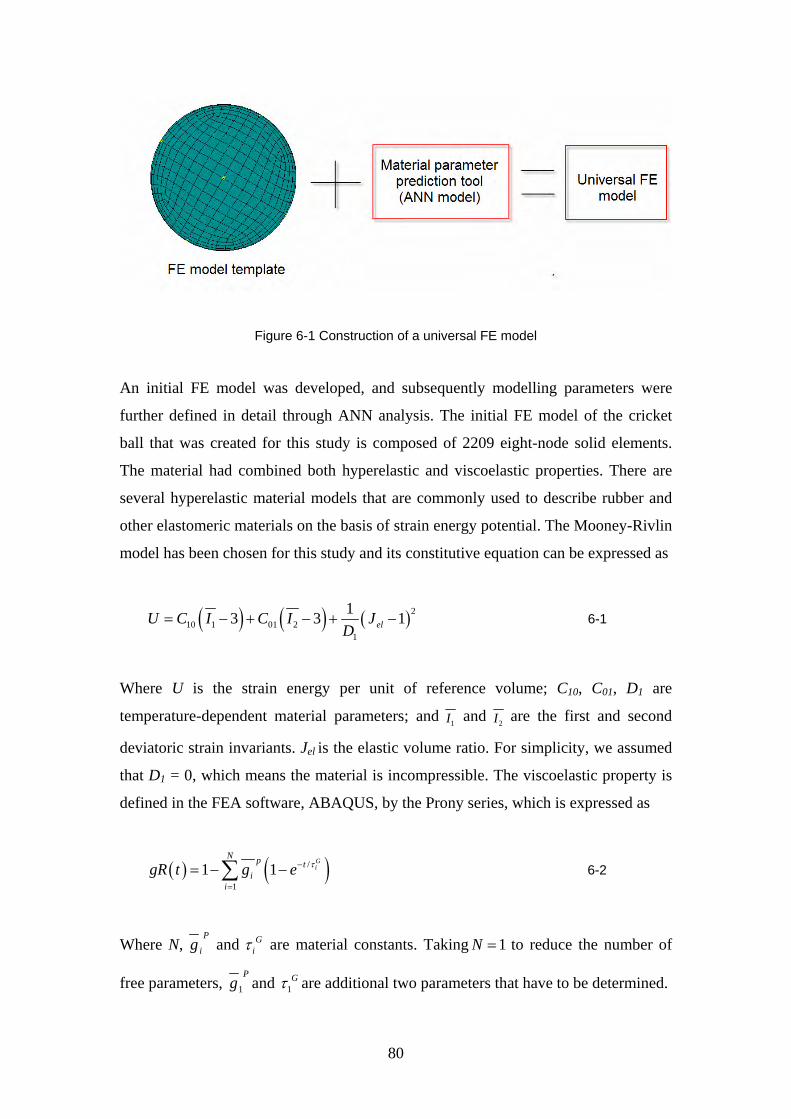
Figure 6-1 Construction of a universal FE model

An initial FE model was developed, and subsequently modelling parameters were

further defined in detail through ANN analysis. The initial FE model of the cricket

ball that was created for this study is composed of 2209 eight-node solid elements.

The material had combined both hyperelastic and viscoelastic properties. There are

several hyperelastic material models that are commonly used to describe rubber and

other elastomeric materials on the basis of strain energy potential. The Mooney-Rivlin

model has been chosen for this study and its constitutive equation can be expressed as

( ) ( ) ( )210 1 01 2

1

13 3 1elU C I C I JD

= − + − + − 6-1

Where U is the strain energy per unit of reference volume; C10, C01, D1 are

temperature-dependent material parameters; and 1I and 2I are the first and second

deviatoric strain invariants. Jel is the elastic volume ratio. For simplicity, we assumed

that D1 = 0, which means the material is incompressible. The viscoelastic property is

defined in the FEA software, ABAQUS, by the Prony series, which is expressed as

( ) ( )/

11 1

Gi

N p ti

igR t g e τ−

=

= − −∑ 6-2

Where N, P

ig and Giτ are material constants. Taking 1N = to reduce the number of

free parameters, 1

Pg and 1

Gτ are additional two parameters that have to be determined.

81

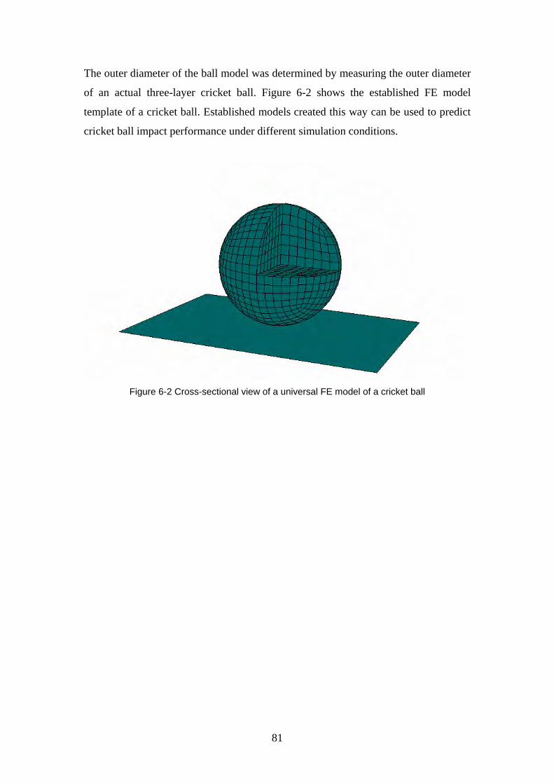
The outer diameter of the ball model was determined by measuring the outer diameter

of an actual three-layer cricket ball. Figure 6-2 shows the established FE model

template of a cricket ball. Established models created this way can be used to predict

cricket ball impact performance under different simulation conditions.

Figure 6-2 Cross-sectional view of a universal FE model of a cricket ball

82

6.2. ANN model development

ANN models are simplified mathematical models of biological neural systems. They

have a strong ability to describe non-linear, multi-model systems by analysing the

changes in the outputs with respect to the changes in the inputs.

The initial FE model is considered as an input and output system, where inputs are

model-produced impact behaviour and outputs are material parameters that define the

FE model. The ANN model can emulate this system. Once the ANN model is

established accurately enough, the output parameters that are the material parameters

can be predicted by providing the input parameters measured from real experiments.

Incorporating the ANN model with an FE model template allows a complete FE

model to be developed

In an FE model, depending on the constitutional equations chosen, there are a few

material parameters that need to be specified. In this study, the cricket ball was

modelled as a solid sphere with hyperelastic and viscoelastic properties. Taking into

account the fact that the material parameters are functions of the impact speed, there

are five parameters that need to be determined. These five parameters are treated as

output parameters and they are C10, C01, 1

Pg , 1

Gτ and impact speed.

In this study, data mining has been devised to describe better the full characteristics of

ball-barrier impact behaviour. As shown in table 6-1, the system approximation is

quantified by 19 key characteristic values that were obtained from the impact force-

time curve and the value of the COR. These 19 principal parameters are treated as

input parameters, as detailed in table 6-1 below.

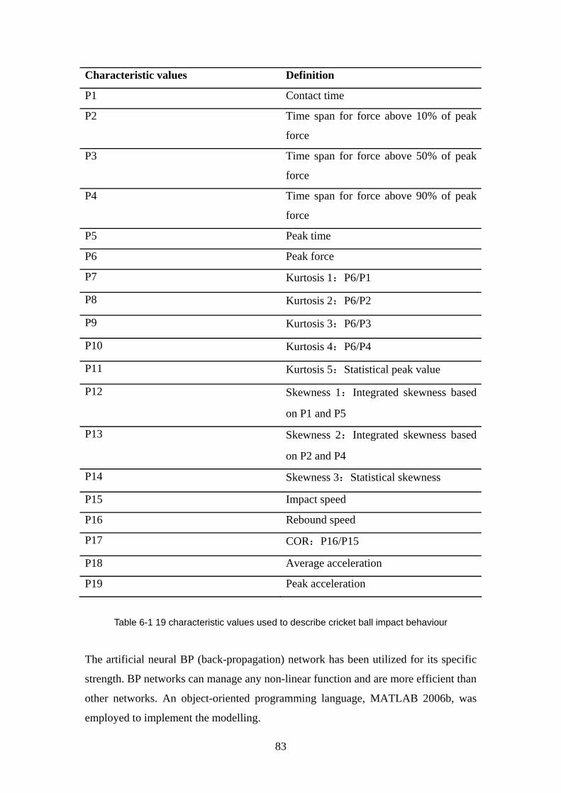
83

Characteristic values Definition

P1 Contact time

P2 Time span for force above 10% of peak

force

P3 Time span for force above 50% of peak

force

P4 Time span for force above 90% of peak

force

P5 Peak time

P6 Peak force

P7 Kurtosis 1：P6/P1

P8 Kurtosis 2：P6/P2

P9 Kurtosis 3：P6/P3

P10 Kurtosis 4：P6/P4

P11 Kurtosis 5：Statistical peak value

P12 Skewness 1：Integrated skewness based

on P1 and P5

P13 Skewness 2：Integrated skewness based

on P2 and P4

P14 Skewness 3：Statistical skewness

P15 Impact speed

P16 Rebound speed

P17 COR：P16/P15

P18 Average acceleration

P19 Peak acceleration

Table 6-1 19 characteristic values used to describe cricket ball impact behaviour

The artificial neural BP (back-propagation) network has been utilized for its specific

strength. BP networks can manage any non-linear function and are more efficient than

other networks. An object-oriented programming language, MATLAB 2006b, was

employed to implement the modelling.

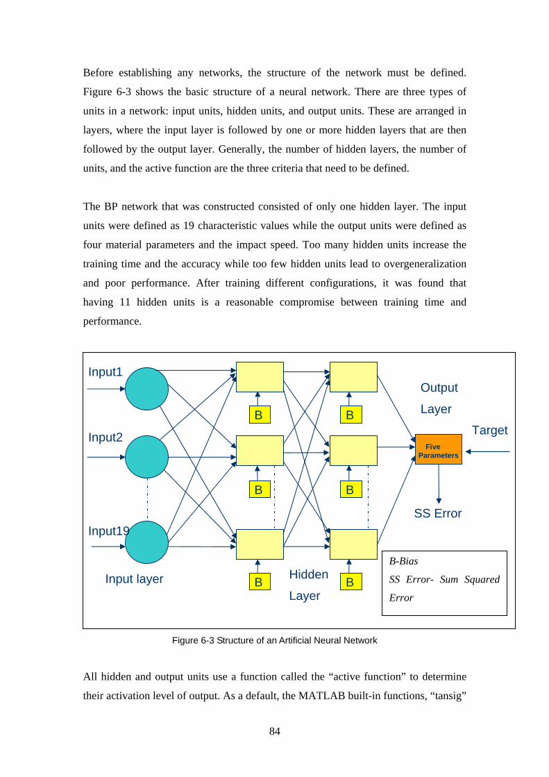
84

Before establishing any networks, the structure of the network must be defined.

Figure 6-3 shows the basic structure of a neural network. There are three types of

units in a network: input units, hidden units, and output units. These are arranged in

layers, where the input layer is followed by one or more hidden layers that are then

followed by the output layer. Generally, the number of hidden layers, the number of

units, and the active function are the three criteria that need to be defined.

The BP network that was constructed consisted of only one hidden layer. The input

units were defined as 19 characteristic values while the output units were defined as

four material parameters and the impact speed. Too many hidden units increase the

training time and the accuracy while too few hidden units lead to overgeneralization

and poor performance. After training different configurations, it was found that

having 11 hidden units is a reasonable compromise between training time and

performance.

Figure 6-3 Structure of an Artificial Neural Network

All hidden and output units use a function called the “active function” to determine

their activation level of output. As a default, the MATLAB built-in functions, “tansig”

B

Input1

Input2

Input19

Input layer

Output

Layer

SS Error

Five

Parameters

Target

Hidden

Layer

B-Bias

SS Error- Sum Squared

Error

B

B B

B B

85

and “purelin”, were chosen for calculating the hidden layer and the output layer

respectively.

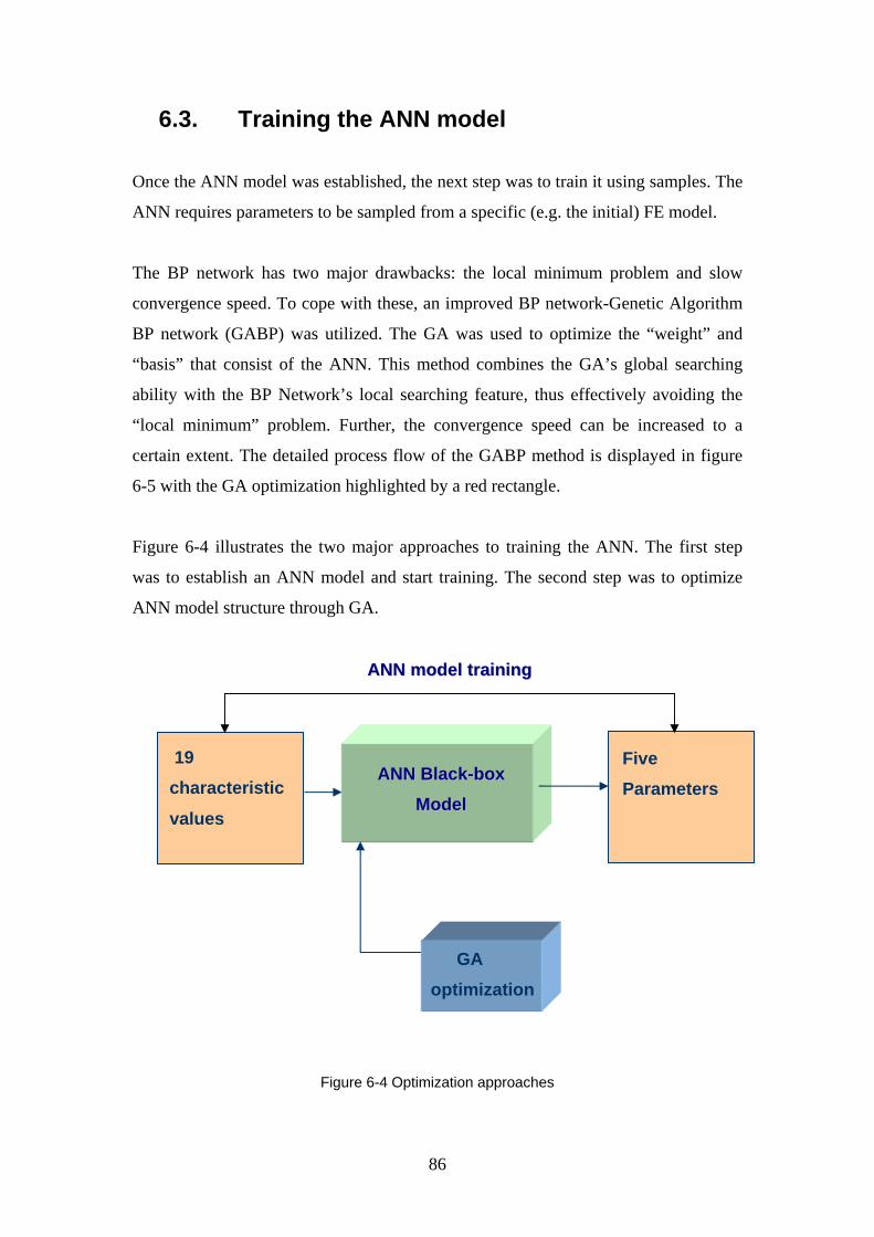
86

6.3. Training the ANN model

Once the ANN model was established, the next step was to train it using samples. The

ANN requires parameters to be sampled from a specific (e.g. the initial) FE model.

The BP network has two major drawbacks: the local minimum problem and slow

convergence speed. To cope with these, an improved BP network-Genetic Algorithm

BP network (GABP) was utilized. The GA was used to optimize the “weight” and

“basis” that consist of the ANN. This method combines the GA’s global searching

ability with the BP Network’s local searching feature, thus effectively avoiding the

“local minimum” problem. Further, the convergence speed can be increased to a

certain extent. The detailed process flow of the GABP method is displayed in figure

6-5 with the GA optimization highlighted by a red rectangle.

Figure 6-4 illustrates the two major approaches to training the ANN. The first step

was to establish an ANN model and start training. The second step was to optimize

ANN model structure through GA.

Figure 6-4 Optimization approaches

19 characteristic

values

AANNNN BBllaacckk--bbooxx

MMooddeell

GA optimization

Five Parameters

AANNNN mmooddeell ttrraaiinniinngg

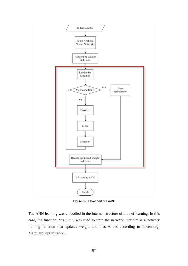
87

Figure 6-5 Flowchart of GABP

The ANN learning was embodied in the internal structure of the net-learning. In this

case, the function, “trainlm”, was used to train the network. Trainlm is a network

training function that updates weight and bias values according to Levenberg-

Marquardt optimization.

88

The training of the network continued until specific criteria were met. The first

criterion trained the network until the sum-squared error (SSE) dropped below the

preset threshold level of 0.005. The learning rate was defined as 0.01 and the

maximum epochs was 3000. Figure 6-6 illustrates the results of a typical GABP

training run. It shows that the SSE drops to the designed threshold of 0.005 after 34

epochs.

Figure 6-6 ANN model training result

Ultimately, over 600 training samples were generated through the use of

modeFRONTIER’s Design of Experiment (DoE) toolbox. These samples represent

different combinations of the five principle parameters, which form the available

design space. The subsequent simulations were processed by the ABAQUS

parametric studies function. The entire process was driven by a tool specially

developed for this study, which enables the batch processing of the sample data. The

ABAQUS parametric studies function is a built-in function that allows the execution

and the gathering of the results of multiple analyses that differ only in the values of

some of the parameters used in place of input quantities. Table 6-2 summarizes the

varying ranges that were used to generate training samples.

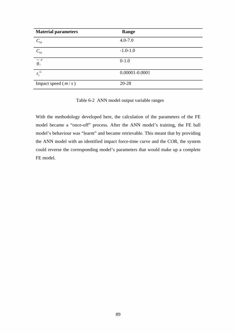
89

Material parameters Range

10C 4.0-7.0

01C -1.0-1.0

1

Pg 0-1.0

1Gτ 0.00001-0.0001

Impact speed ( /m s ) 20-28

Table 6-2 ANN model output variable ranges

With the methodology developed here, the calculation of the parameters of the FE

model became a “once-off” process. After the ANN model’s training, the FE ball

model’s behaviour was “learnt” and became retrievable. This meant that by providing

the ANN model with an identified impact force-time curve and the COR, the system

could reverse the corresponding model’s parameters that would make up a complete

FE model.

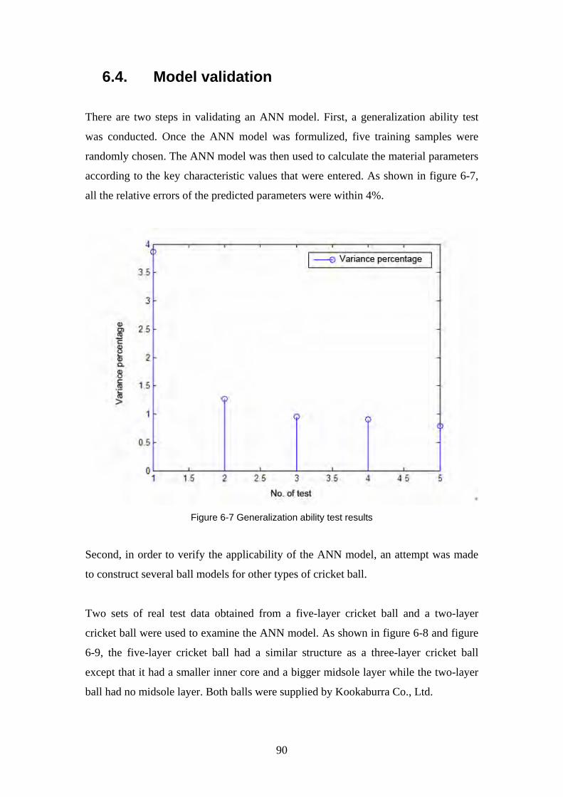
90

6.4. Model validation

There are two steps in validating an ANN model. First, a generalization ability test

was conducted. Once the ANN model was formulized, five training samples were

randomly chosen. The ANN model was then used to calculate the material parameters

according to the key characteristic values that were entered. As shown in figure 6-7,

all the relative errors of the predicted parameters were within 4%.

Figure 6-7 Generalization ability test results

Second, in order to verify the applicability of the ANN model, an attempt was made

to construct several ball models for other types of cricket ball.

Two sets of real test data obtained from a five-layer cricket ball and a two-layer

cricket ball were used to examine the ANN model. As shown in figure 6-8 and figure

6-9, the five-layer cricket ball had a similar structure as a three-layer cricket ball

except that it had a smaller inner core and a bigger midsole layer while the two-layer

ball had no midsole layer. Both balls were supplied by Kookaburra Co., Ltd.

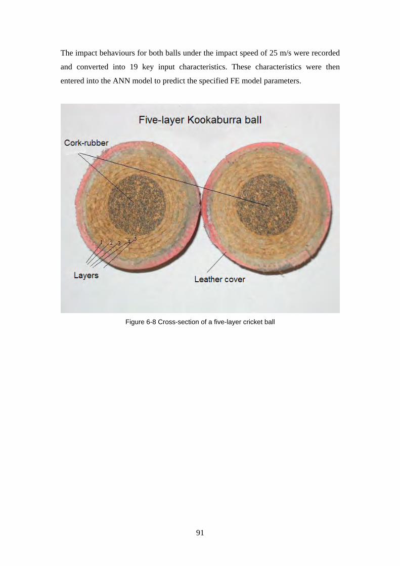
91

The impact behaviours for both balls under the impact speed of 25 m/s were recorded

and converted into 19 key input characteristics. These characteristics were then

entered into the ANN model to predict the specified FE model parameters.

Figure 6-8 Cross-section of a five-layer cricket ball

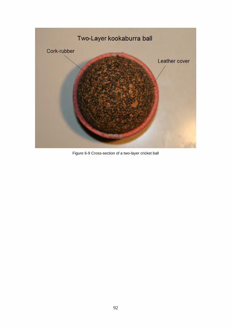
92

Figure 6-9 Cross-section of a two-layer cricket ball

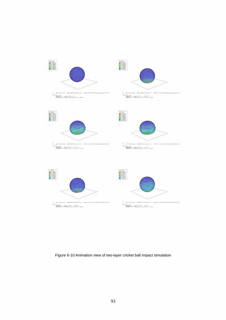
93

Figure 6-10 Animation view of two-layer cricket ball impact simulation

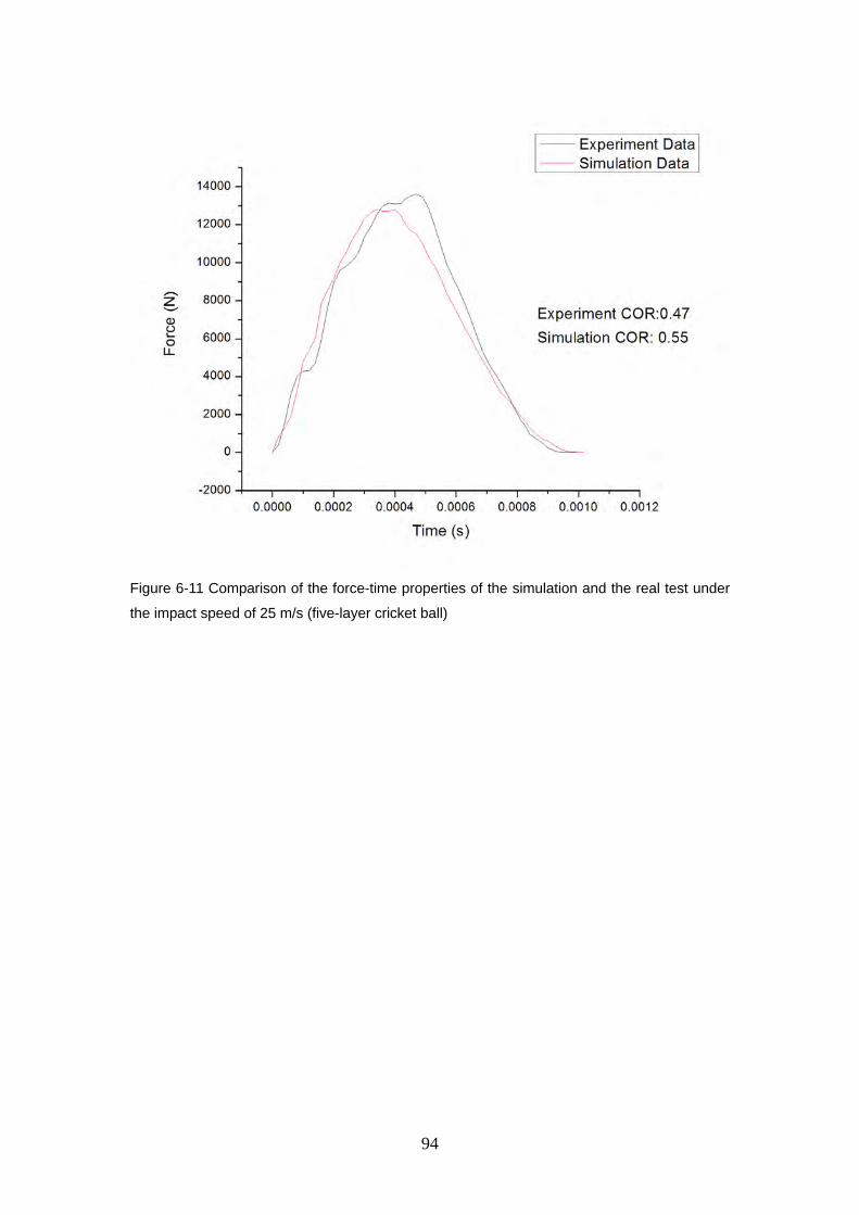
94

Figure 6-11 Comparison of the force-time properties of the simulation and the real test under

the impact speed of 25 m/s (five-layer cricket ball)

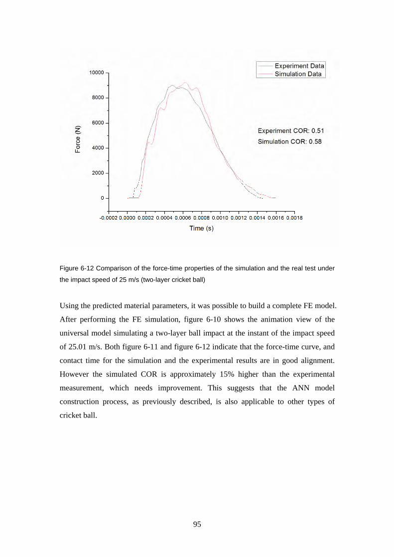
95

Figure 6-12 Comparison of the force-time properties of the simulation and the real test under

the impact speed of 25 m/s (two-layer cricket ball)

Using the predicted material parameters, it was possible to build a complete FE model.

After performing the FE simulation, figure 6-10 shows the animation view of the

universal model simulating a two-layer ball impact at the instant of the impact speed

of 25.01 m/s. Both figure 6-11 and figure 6-12 indicate that the force-time curve, and

contact time for the simulation and the experimental results are in good alignment.

However the simulated COR is approximately 15% higher than the experimental

measurement, which needs improvement. This suggests that the ANN model

construction process, as previously described, is also applicable to other types of

cricket ball.

96

7. Results and Discussion

7.1. Introduction

This chapter summarizes the experimental results and compares these results with

those from the various numerical models that have been developed in this study.

Three types of Kookaburra cricket balls have been examined: a two-layer solid ball, a

three-layer ball, and a five-layer ball. Each ball was tested over a speed range of 5m/s

to 25 m/s. The tests used both drop test and high speed impact test rigs. In addition,

the core unit and the cork unit that were taken out of a three-layer cricket ball have

also been tested at the impact speed of 20.8 m/s for the purpose of verifying the

detailed FE model.

The coefficient of restitution (COR) and the dynamic impact load are the two

properties that are most commonly used to describe a sports ball undergoing impact.

This chapter is mainly concerned with how both the COR and the dynamic impact

load change in relation to impact speed. The comparison between the experimental

results and simulation results was only conducted on three-layer cricket ball.

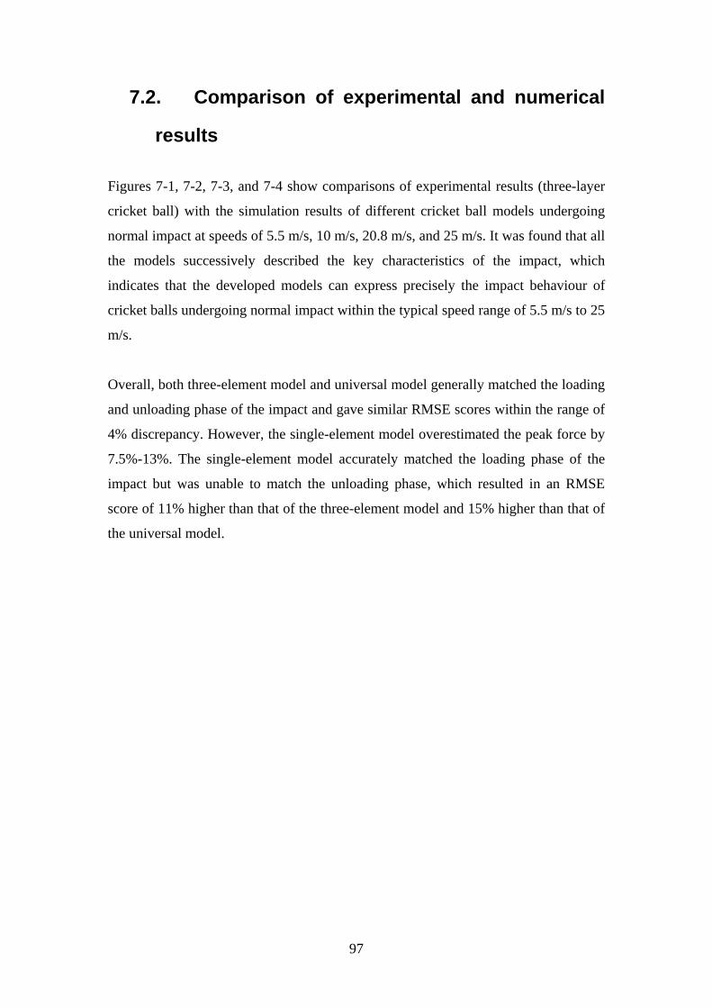
97

7.2. Comparison of experimental and numerical

results

Figures 7-1, 7-2, 7-3, and 7-4 show comparisons of experimental results (three-layer

cricket ball) with the simulation results of different cricket ball models undergoing

normal impact at speeds of 5.5 m/s, 10 m/s, 20.8 m/s, and 25 m/s. It was found that all

the models successively described the key characteristics of the impact, which

indicates that the developed models can express precisely the impact behaviour of

cricket balls undergoing normal impact within the typical speed range of 5.5 m/s to 25

m/s.

Overall, both three-element model and universal model generally matched the loading

and unloading phase of the impact and gave similar RMSE scores within the range of

4% discrepancy. However, the single-element model overestimated the peak force by

7.5%-13%. The single-element model accurately matched the loading phase of the

impact but was unable to match the unloading phase, which resulted in an RMSE

score of 11% higher than that of the three-element model and 15% higher than that of

the universal model.

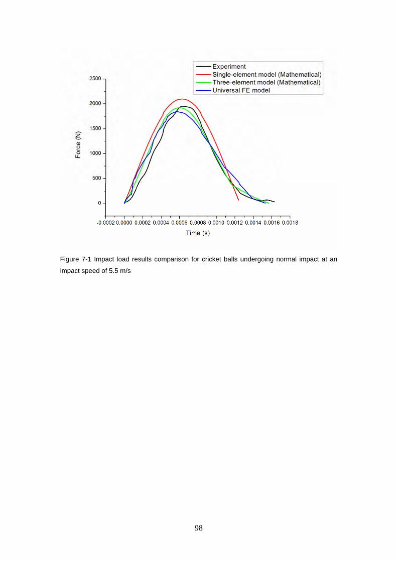
98

Figure 7-1 Impact load results comparison for cricket balls undergoing normal impact at an

impact speed of 5.5 m/s

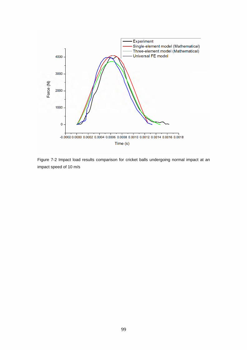
99

Figure 7-2 Impact load results comparison for cricket balls undergoing normal impact at an

impact speed of 10 m/s

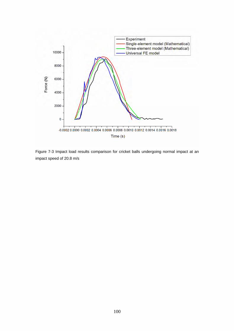
100

Figure 7-3 Impact load results comparison for cricket balls undergoing normal impact at an

impact speed of 20.8 m/s

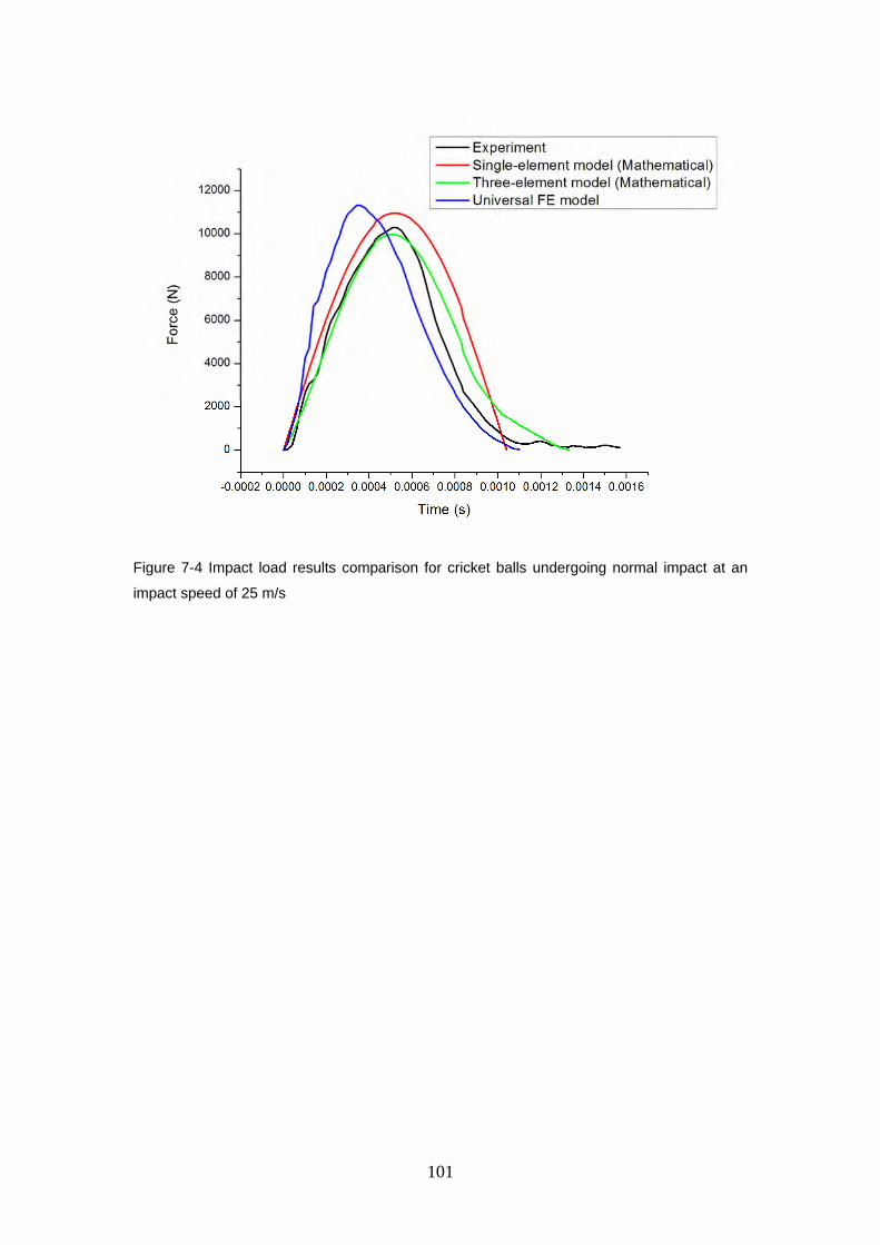
101

Figure 7-4 Impact load results comparison for cricket balls undergoing normal impact at an

impact speed of 25 m/s

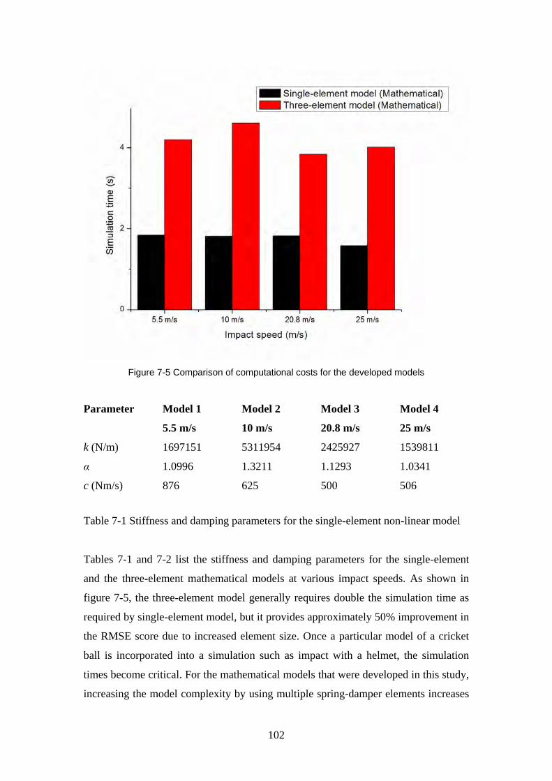
102

Figure 7-5 Comparison of computational costs for the developed models

Parameter Model 1

5.5 m/s

Model 2

10 m/s

Model 3

20.8 m/s

Model 4

25 m/s

k (N/m) 1697151 5311954 2425927 1539811

α 1.0996 1.3211 1.1293 1.0341

c (Nm/s) 876 625 500 506

Table 7-1 Stiffness and damping parameters for the single-element non-linear model

Tables 7-1 and 7-2 list the stiffness and damping parameters for the single-element

and the three-element mathematical models at various impact speeds. As shown in

figure 7-5, the three-element model generally requires double the simulation time as

required by single-element model, but it provides approximately 50% improvement in

the RMSE score due to increased element size. Once a particular model of a cricket

ball is incorporated into a simulation such as impact with a helmet, the simulation

times become critical. For the mathematical models that were developed in this study,

increasing the model complexity by using multiple spring-damper elements increases

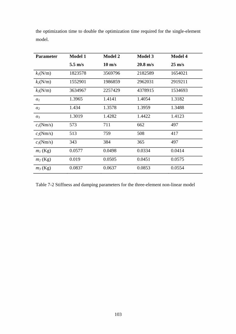
103

the optimization time to double the optimization time required for the single-element

model.

Parameter Model 1

5.5 m/s

Model 2

10 m/s

Model 3

20.8 m/s

Model 4

25 m/s

k1(N/m) 1823578 3569796 2182589 1654021

k2(N/m) 1552901 1986859 2962031 2919211

k3(N/m) 3634967 2257429 4378915 1534693

α1 1.3965 1.4141 1.4054 1.3182

α2 1.434 1.3578 1.3959 1.3488

α3 1.3019 1.4282 1.4422 1.4123

c1(Nm/s) 573 711 662 497

c2(Nm/s) 513 759 508 417

c3(Nm/s) 343 384 365 497

m1 (Kg) 0.0577 0.0498 0.0334 0.0414

m2 (Kg) 0.019 0.0505 0.0451 0.0575

m3 (Kg) 0.0837 0.0637 0.0853 0.0554

Table 7-2 Stiffness and damping parameters for the three-element non-linear model

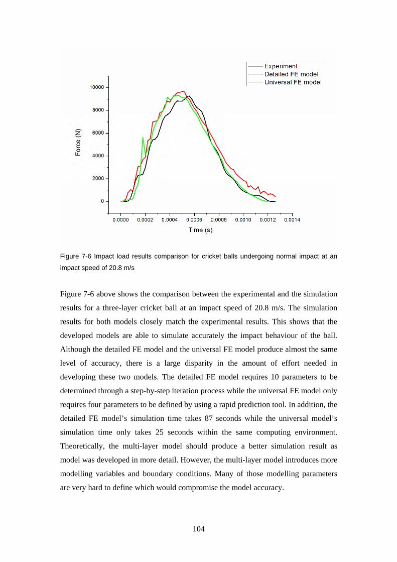
104

Figure 7-6 Impact load results comparison for cricket balls undergoing normal impact at an

impact speed of 20.8 m/s

Figure 7-6 above shows the comparison between the experimental and the simulation

results for a three-layer cricket ball at an impact speed of 20.8 m/s. The simulation

results for both models closely match the experimental results. This shows that the

developed models are able to simulate accurately the impact behaviour of the ball.

Although the detailed FE model and the universal FE model produce almost the same

level of accuracy, there is a large disparity in the amount of effort needed in

developing these two models. The detailed FE model requires 10 parameters to be

determined through a step-by-step iteration process while the universal FE model only

requires four parameters to be defined by using a rapid prediction tool. In addition, the

detailed FE model’s simulation time takes 87 seconds while the universal model’s

simulation time only takes 25 seconds within the same computing environment.

Theoretically, the multi-layer model should produce a better simulation result as

model was developed in more detail. However, the multi-layer model introduces more

modelling variables and boundary conditions. Many of those modelling parameters

are very hard to define which would compromise the model accuracy.

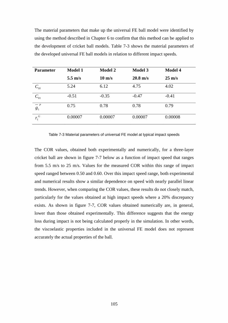
105

The material parameters that make up the universal FE ball model were identified by

using the method described in Chapter 6 to confirm that this method can be applied to

the development of cricket ball models. Table 7-3 shows the material parameters of

the developed universal FE ball models in relation to different impact speeds.

Parameter Model 1

5.5 m/s

Model 2

10 m/s

Model 3

20.8 m/s

Model 4

25 m/s

10C 5.24 6.12 4.75 4.02

01C -0.51 -0.35 -0.47 -0.41

1

Pg 0.75 0.78 0.78 0.79

1Gτ 0.00007 0.00007 0.00007 0.00008

Table 7-3 Material parameters of universal FE model at typical impact speeds

The COR values, obtained both experimentally and numerically, for a three-layer

cricket ball are shown in figure 7-7 below as a function of impact speed that ranges

from 5.5 m/s to 25 m/s. Values for the measured COR within this range of impact

speed ranged between 0.50 and 0.60. Over this impact speed range, both experimental

and numerical results show a similar dependence on speed with nearly parallel linear

trends. However, when comparing the COR values, these results do not closely match,

particularly for the values obtained at high impact speeds where a 20% discrepancy

exists. As shown in figure 7-7, COR values obtained numerically are, in general,

lower than those obtained experimentally. This difference suggests that the energy

loss during impact is not being calculated properly in the simulation. In other words,

the viscoelastic properties included in the universal FE model does not represent

accurately the actual properties of the ball.

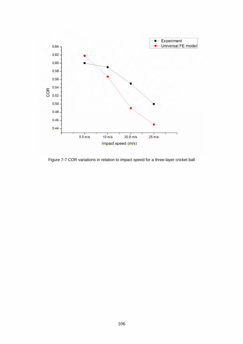
106

Figure 7-7 COR variations in relation to impact speed for a three-layer cricket ball

107

Figure 7-8 High speed video images

Figure 7-8 shows the high speed video image taken from a normal impact test

conducted on a three-layer cricket ball at an impact speed of 25 m/s. Figures 7-9 and

7-10 show the corresponding simulations by using the detailed FE models and the

universal model respectively. In spite of the high computing cost, the detailed FE

model can serve as a useful tool if the focus is on the ball itself. This model could be

used to investigate many other aspects of the ball that are difficult to obtain

experimentally, such as the internal characteristics of the ball. For example, the model

can be used to examine the effect of the inner material properties on the impact load

history and the COR of the ball.

The animated view of ball impact using the universal FE model is shown in figure 7-

10, which represents the results of explicit dynamic finite element analysis. Compared

to the detailed FE model, the universal FE model is a relatively cost-effective

technique for simulating the impact behaviour of a cricket ball. A potential downside

of the universal FE model is the numerical instability due to the nature of ANN

modelling techniques. In some cases, the ANN model may need several runs to

108

achieve a reasonable solution of the material parameters. Besides, the development of

such a universal FE model requires a large amount of preparation work, such as the

design of experiments and FE simulation iteration, to establish the impact behaviour

database of the ball that is being tested.

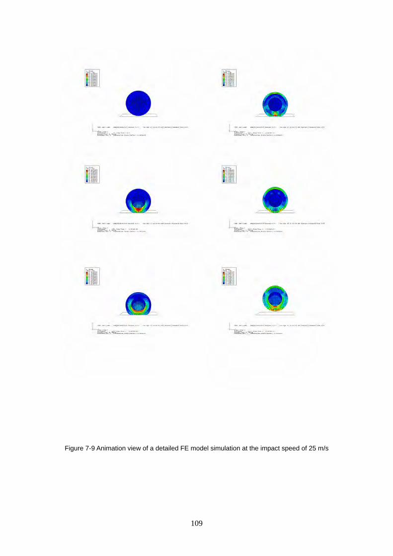
109

Figure 7-9 Animation view of a detailed FE model simulation at the impact speed of 25 m/s

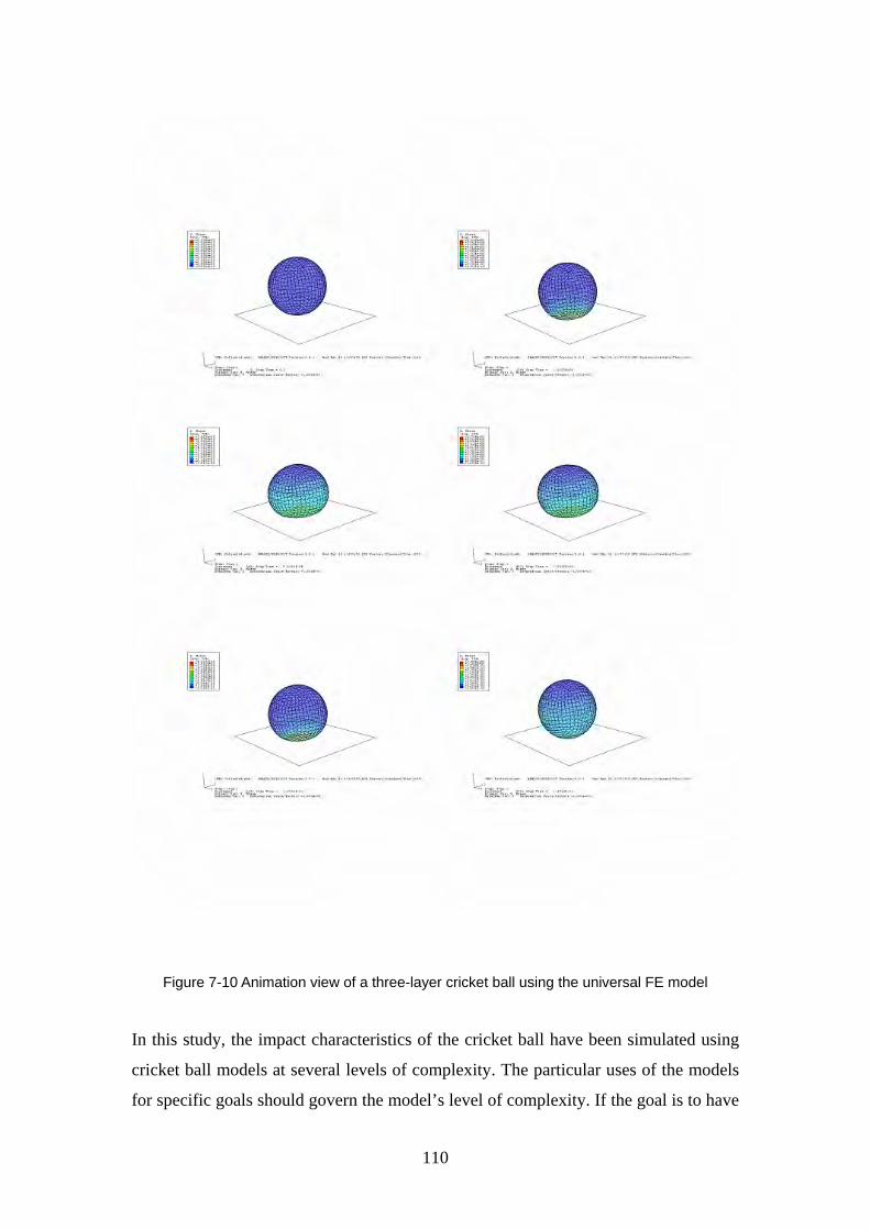
110

Figure 7-10 Animation view of a three-layer cricket ball using the universal FE model

In this study, the impact characteristics of the cricket ball have been simulated using

cricket ball models at several levels of complexity. The particular uses of the models

for specific goals should govern the model’s level of complexity. If the goal is to have

111

an accurate three-dimensional model, then a universal model is the appropriate choice.

However, if the model is intended to be used as part of a larger model, a simpler

model such as a single-element model or a three-element model may be more suitable.

A significant outcome from this study was the derivation of the universal FE model.

This model is important in relation to the growing interest in the development of

sports equipment for cricket, as this model can provide rapid ball model development

with relatively low computing costs and high accuracy.

112

8. Conclusion

In cricket, high speed impacts occur between the cricket ball and the bat, player and

their protective equipment. Improved understanding of impact dynamics has the

potential to significantly improve the development of cricket equipment and also

contribute to improving the player’s safety and performance. In particular,

development of high performance cricket balls with enhanced structural properties

(e.g. improved durability) would benefit greatly from such insight.

In order to gain more insight into the impact dynamics of cricket balls, appropriate

structural models of the ball are required. This study introduced two fast-solving

numerical models, a detailed FE model and a universal FE model, for the structural

analysis of cricket balls. The models were derived using experimental data obtained

from tests developed for this purpose, including drop tests and high speed impact tests.

The experimental work presented in this study included measurements of impact

behaviour of two-layer, three-layer, and five-layer cricket balls using a dynamic

signal analyser and high speed video analysis software. The ball properties obtained

experimentally were then used to develop two mathematical models: a single-element

model and a three-element model. These cricket ball models have been developed so

that they capture the key characteristics of ball-impact behaviour while allowing for

fast-solving dynamic simulation. The stiffness and damping properties of both models

were determined using a novel fast-solving genetic algorithm. These models predict

the force-time diagram during impact with very little computing cost. However,

developing a mathematical model with a reasonable level of accuracy is still a

challenge.

The simulation of the ball model impact with a flat surface achieved reasonable

agreement with experimental results for both the single-element and the three-element

models. The genetic algorithm (GA) method proved to be more efficient and

convenient than directly solving the differential equations.

113

This project successfully delivered a multi-layer and multi-material cricket ball model

with high accuracy. The intended use for such a model is to provide accurate results

that incorporate the geometry of the cricket ball and area deformation characteristics.

This model can also be used as a valuable tool to enable manufacturers to discover

and synthesize new materials and new designs for cricket balls. Furthermore, the

application presented here can be extended to simulate any solid ball impact. To

determine the material parameters within this model, this study developed a highly

automated approach that significantly reduced the amount of handwork required.

Comparison of the simulation results and the experimental results reveals that the

force-time curve and the contact time are both in good alignment. However, the COR

that was predicted by the model and the COR obtained from the experiment do not

match closely. This is probably because the initial values of the material parameters

were of poor quality. Manual fine-tuning or adopting better numerical optimization

methods are possible ways of improving this model.

An initial attempt was made to extend the applications of the detailed FE model to

include the prediction of oblique impacts. The attempt demonstrated the potential ease

with which the FE model developed in this study can be extended to predict an

oblique impact.

A universal finite element (FE) ball model was developed within the ABAQUS CAE

environment. This model can be seen as a combination of an FE model template and a

material parameter selection tool based on an Artificial Neural Network (ANN) model.

This approach allows for rapid model development while producing accurate results

at different impact speeds. Two sets of real test data obtained from a five-layer cricket

ball and a two-layer cricket ball at impact velocity of 25.01 m/s were used to examine

the ANN model. Comparison of results shows good agreement between the

simulation results and the experimental results.

An important feature of the developed universal FE model is its flexibility. The results

show that the developed FE-ANN model can be used to predict the impact behaviour

of different types of cricket ball under various dynamic conditions. This flexibility

represents an advantage that can be utilized by sports equipment developers to rapidly

develop different cricket ball models needed for inclusion in larger simulations

114

involving impact of a cricket ball with other objects. The developed FE-ANN model

and the corresponding training process represent an invaluable tool for facilitating

design, analysis and structural optimization of cricket-related sports equipment.

8.1. Future directions

a) This study was limited to the assessment of ball impact behaviour at impact speeds

of less than 25 m/s, while under actual game conditions, the maximum impact speed

may reach up to 45 m/s. Therefore, future studies are needed in this area.

b) Oblique impact behaviour of cricket balls was not considered much in this study

due to the lack of experimental facilities. It is estimated that ball sliding and ball

rolling on the target surface, in addition to ball deformation, could occur during

impact. Precisely predicting this complex interaction would require the introduction

of several frictional characteristics between the ball and the target. Such a model with

detailed frictional characteristics can potentially expand the applications of the model

developed in this study.

c) Material parameters studies can be conducted on the established detailed FE model.

This will enable further investigation of the performance characteristics of cricket

balls and the effect that changes to the material parameters have on the impact load

pulse and the COR.

d) While developing the detailed FE model, the contact definition between layers was

defined as “hard” contact for simplicity. To take the friction between the layers into

account, further studies would be required.

e) Although the results of the universal model were encouraging, the universal model

has a heritage limitation as it heavily relies on the samples (design space) that were

used for ANN training. Good results can only be expected when the design space

covers the range of those material parameters that are going to be identified. Further

validation of this model would be necessary to account for other factors before it can

be used confidently. It is believed that further development of the design space can

115

increase the performance of the universal model as well as its simulation accuracy.

Further studies are also needed to discover the relationships between inputs and

outputs that could add greater accuracy to the predictions. For example, give different

weight to the 19 principal parameters, as obviously the contact time, shape of the

force-time curve and average acceleration should be of less importance than the ball

COR or peak force.

f) Due to time limitation, the effect of mesh refinement was not considered in this

study. It would be worthwhile to conduct such a convergence study in the future,

especially when the ball model would be incorporated in a non-flat surface impact

simulation

116

References

CARRÉ, M. J., JAMES, D. M. & HAAKE, S. J. (2004) Impact of a non-homogeneous sphere on a rigid surface. Proceedings of the Institution of Mechanical Engineers, 218, 273-281.

CRISCO, J. J., HENDEE, S. P. & GREENWALD, R. M. (1997) The influence of baseball modulus and mass on head and chest impacts: A theoretical study. Medicine & Science in Sports & Exercise, 29, 26-36.

CROSS, R. (1999) The bounce of a ball. American Journal of Physics, Vol.67, 222-227 DAISH, C. B. (1972) The physics of ball games, London, The English University Press. DIGNALL, R. J. & HAAKE, S. J. (2000) Analytical modelling of the impact of tennis balls on

court surfaces. Medicine and Science in Tennis. Blackwell Science Ltd. London DURIS, J. G. (2004) Experimental and Numerical Characterization of Softballs Department of Mechanical and Materials Engineering. Washington, Washington State

University. GOBUSH, W. (1990) Impact force measurement on golf balls IN COCHRAN, A. J. &

FARRALLY, M. R. (Eds.) Science and Golf I: Proceedings of the World Scientific Congress of Golf.

HERRMANN, L. R. & PETERSON, F. E. (1968) A numerical procedure for viscoelastic stress analysis. Seventh Meeting of ICRPG Mechanical Behavior Working Group. Orlando, F.L.

JOHNSON, S. H. & LIEBERMAN, B. B. (1996) Normal impact models for golf balls. The Engineering of Sport. Sheffield, UK.

KANDA, Y., NAGAO, H. & NARUO, T. (2002) Estimation of tennis racket power using three-dimensional finite element analysis. IN UJIHASHI, S. & HAAKE, S. J. (Eds.) The Engineering of Sport 4. Kyoto, Japan, Blackwell Publishing.

LIEBERMAN, B. B. & JOHNSON, S. H. (1994) An analytical model for ball-barrier impart. IN COCHRAN, A. J. & FARRALLY, M. R. (Eds.) 1994 World Scientific Congress of Golf. St. Andrews, Scotland.

MORIYAMA, K., YAMAGUCHI, T., YABU, M. & TSUNODA, M. (2004) The influence of mechanical impedance of the golf club and the golf ball on ball spin. IN HUBBARD, M., MEHTA, R. D. & PALLIS, J. M. (Eds.) The Engineering of Sport 5. Davis CA, International Sports Engineering Association.

MUSTONE, T. J. & SHERWOOD, J. A. (1998) Using LS-DYNA to characterize the performance of baseball bats. 5th International LS-DYNA User's Conference. Detroit, M.I.

NATHAN, A. M. (2000) Dynamics of the baseball-bat collision. American Journal of Physics, 68, 979-990.

NICHOLLS, R. L. (2003) Mathematical modelling of bat-ball Impact in baseball. School of Human Movement and Exercise Science, School of Mechanical Engineering. University of Western Australia.

NICHOLLS, R. L., MILLERA, K. & ELLIOTT, B. C. (2005) Numerical analysis of maximal bat performance in baseball. Journal of Biomechanics, 4, 65-74.

SAYERS, A. T. & HILL, A. (1999) Aerodynamics of a cricket ball. Journal of wind engineering and Industrial aerodynamics, vol.79, 169-182.

SHENOY, M. M., SMITH, L. V. & AXTELL, J. T. (2001) Performance assessment of wood, metal and composite baseball bats. Composite Structures, 52, 397-404.

SIMON, R. (1967) The development of a mathematical tool for evaluating golf club performance. ASME Design Engineering Conference. New York.

SMITH, L. V. (2001) Evaluating baseball bat performance. Sports Engineering, 4, 205-214. SMITH, L. V., SHENOY, M. & AXTELL, J. T. (2000) Simulated composite baseball bat impacts

using numerical and experimental techniques. Society for Experimental Mechanics, Spring Conference. Orlando, F.L.

SUBIC, A., TAKLA, M. & KOVAS, J. (2005) Modelling and analysis of alternative face guard designs for cricket using finite element modelling. Sports Engineering, 8, 209-222.

117

TAVARES, G., SULLIVAN, M. & NESBITT, D. (1998) Use of finite element analysis in design of multilayer golf balls. IN MARTIN, R., FARRALLY, A. & COCHRAN, J. (Eds.) Science and Golf III - Proceedings of the World Scientific Congress of Golf. St. Andrews, Scotland.

UJIHASHI, S. (1994) Measurement of dynamic characteristics of golf balls and identification of their mechanical models. IN COCHRAN, A. J. & FARRALLY, M. (Eds.) Science and Golf II: Proceedings of the 1994 World Scientific Congress of Golf. St. Andrews, Scotland

UJIHASHI, S., KONISHI, T. & SATOH, F. (2002) Computer simulations of the oblique impact of golf balls with circular plates of various thickness. IN UJIHASHI, S. & HAAKE, S. J. (Eds.) The Engineering of Sport 4. Kyoto, Japan, Blackwell Publishing

YAMAGUCHI, T. & IWATSUBO, T. (1998) Optimum design of golf club considering the mechanical impedance matching. IN FARRALLY, M. R. & COCHRAN, A. J. (Eds.) Science and Golf III - Proceedings of the World Scientific Congress of Golf. St. Andrews, Scotland.

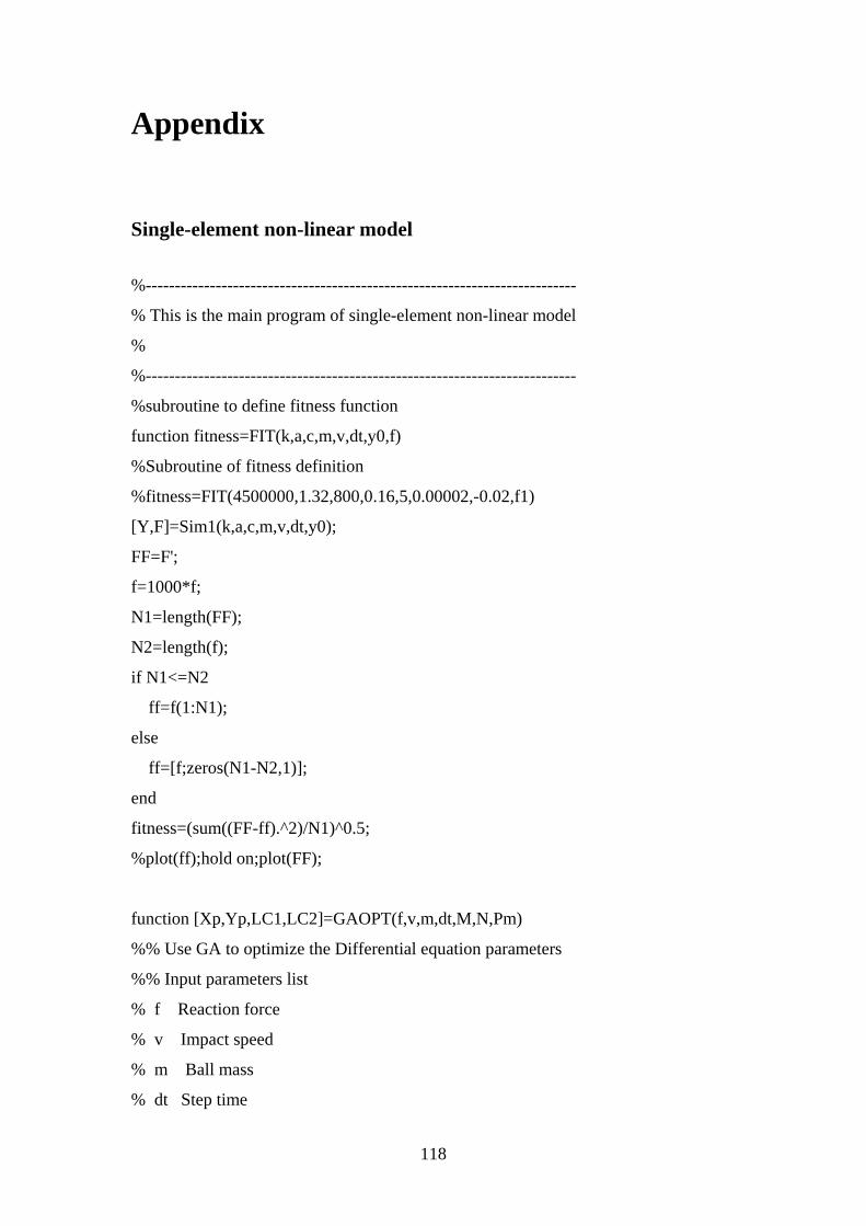
118

Appendix

Single-element non-linear model

%--------------------------------------------------------------------------

% This is the main program of single-element non-linear model

%

%--------------------------------------------------------------------------

%subroutine to define fitness function

function fitness=FIT(k,a,c,m,v,dt,y0,f)

%Subroutine of fitness definition

%fitness=FIT(4500000,1.32,800,0.16,5,0.00002,-0.02,f1)

[Y,F]=Sim1(k,a,c,m,v,dt,y0);

FF=F';

f=1000*f;

N1=length(FF);

N2=length(f);

if N1<=N2

ff=f(1:N1);

else

ff=[f;zeros(N1-N2,1)];

end

fitness=(sum((FF-ff).^2)/N1)^0.5;

%plot(ff);hold on;plot(FF);

function [Xp,Yp,LC1,LC2]=GAOPT(f,v,m,dt,M,N,Pm)

%% Use GA to optimize the Differential equation parameters

%% Input parameters list

% f Reaction force

% v Impact speed

% m Ball mass

% dt Step time

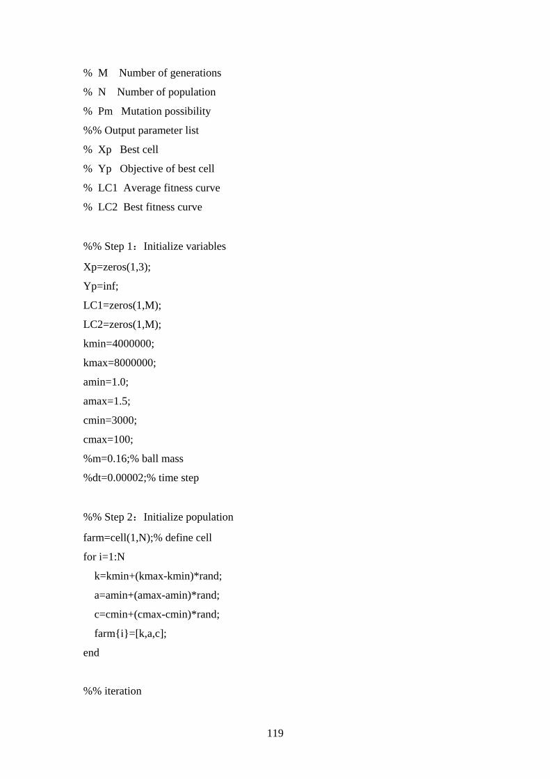
119

% M Number of generations

% N Number of population

% Pm Mutation possibility

%% Output parameter list

% Xp Best cell

% Yp Objective of best cell

% LC1 Average fitness curve

% LC2 Best fitness curve

%% Step 1：Initialize variables

Xp=zeros(1,3);

Yp=inf;

LC1=zeros(1,M);

LC2=zeros(1,M);

kmin=4000000;

kmax=8000000;

amin=1.0;

amax=1.5;

cmin=3000;

cmax=100;

%m=0.16;% ball mass

%dt=0.00002;% time step

%% Step 2：Initialize population

farm=cell(1,N);% define cell

for i=1:N

k=kmin+(kmax-kmin)*rand;

a=amin+(amax-amin)*rand;

c=cmin+(cmax-cmin)*rand;

farm{i}=[k,a,c];

end

%% iteration

120

counter=0;% set counter

while counter<M% cease condition

%% Cross over

%

newfarm=cell(1,2*N);% child cell

Ser=randperm(N);%match list

A=farm{Ser(1)};%farther A

B=farm{Ser(2)};%farther B

pos=rand;

a=pos*A+(1-pos)*B;%child a

b=(1-pos)*A+pos*B;%child b

newfarm{2*N-1}=a;%insert child generation

newfarm{2*N}=b;

for i=1:(N-1)

A=farm{Ser(i)};

B=farm{Ser(i+1)};

pos=rand;

a=pos*A+(1-pos)*B;%child a

b=(1-pos)*A+pos*B;%child b

newfarm{2*i-1}=a;

newfarm{2*i}=b;

end

FARM=[farm,newfarm];% Generation combine

%% Step 4：Clone

SER=randperm(2*N);

FITNESS=zeros(1,2*N);

fitness=zeros(1,N);

for i=1:(2*N)

Beta=FARM{i};

k=Beta(1);

a=Beta(2);

121

c=Beta(3);

FITNESS(i)=FIT(k,a,c,m,v,dt,0,f);% Call fitness function

end

for i=1:N

f1=FITNESS(SER(2*i-1));

f2=FITNESS(SER(2*i));

if f1<=f2

farm{i}=FARM{SER(2*i-1)};

fitness(i)=FITNESS(SER(2*i-1));

else

farm{i}=FARM{SER(2*i)};

fitness(i)=FITNESS(SER(2*i));

end

end

%% Plot

minfitness=min(fitness);

meanfitness=mean(fitness);

if minfitness<Yp

pos=find(fitness==minfitness);

Xp=farm{pos(1)};

Yp=minfitness;

end

LC2(counter+1)=Yp;

LC1(counter+1)=meanfitness;

%% Step 5：Mutation

for i=1:N

if Pm>rand&&pos(1)~=i

AA=farm{i};

POS=unidrnd(3);

if POS==1

AA(POS)=kmin+(kmax-kmin)*rand;

122

elseif POS==2

AA(POS)=amin+(amax-amin)*rand;

elseif POS==3

AA(POS)=cmin+(cmax-cmin)*rand;

else

end

farm{i}=AA;

end

end

%%

counter=counter+1

end

%% Step 7：Plot of convergence curve

figure(1);

plot(LC1);

xlabel('Counter');

ylabel('Fitness average');

title('Average fitness curve');

figure(2);

plot(LC2);

xlabel(' Counter);

ylabel('Best fitness');

title('Best fitnesscurve');

figure(3)

plot(1000*f)

hold on

[Y,F]=Sim1(Xp(1),Xp(2),Xp(3),m,v,dt,0);

F=F';

t=0:(length(F)-1);

T=0.00002*t;

plot(F);

xlabel('time(0.00002s)')

123

ylabel('force(N)')

function [Y,F]=Sim1(k,a,c,m,v,dt,y0)

y1=y0;% position of last time

y2=y1-v*dt;% current position

f1=-sign(y2-y0)*k*(abs(y2-y0))^a;% elastic force

f=f1;% total force

A=f/m;% acceleration

v=v-A*dt;% update of velocity

counter=0;

Y=[y1,y2];

F=f;

while y2<y0

y1=y2;

y2=y1-v*dt;

f1=-sign(y2-y0)*k*(abs(y2-y0))^a;

if y2>=y1

f2=-c*(abs(y2-y1));

else

f2=0;

end

f=f1+f2;

A=f/m;

v=v-A*dt;

Y=[Y,y2];

F=[F,f];

counter=counter+1;

end

F1=F(1);

F2=F(end);

Fmax=max([F1,F2]);

pos=find(F>=Fmax);

F=F(pos)-Fmax;

124

Three-element non-linear model

%--------------------------------------------------------------------------

% This is the main program of three-element non-linear model

%

%--------------------------------------------------------------------------

function [Xp,Yp,LC1,LC2]=GAOPT(f,v,m,dt,M,N,Pm)

%% use GA to optimize differential equation parameters

%% Input list

% f real force

% v impact speed

% m ball mass

% dt time step

% M Number of generation

% N Number of population

% Pm Mutation possibility

%% output list

% Xp Best cell

% Yp Objective of best cell

% LC1 Average fitness curve

% LC2 Best fitness curve

%% Step1：Initialize variables

Xp=zeros(1,12);

Yp=inf;

LC1=zeros(1,M);

LC2=zeros(1,M);

kmin=4000000;

kmax=8000000;

amin=1.0;

amax=1.5;

cmin=3000;

cmax=100;

%m=0.16;% ball mass

125

%dt=0.00002;% time step

%% Step 2：Randomize initial population

farm=cell(1,N);% define cell

for i=1:N

k1=kmin+(kmax-kmin)*rand;

k2=kmin+(kmax-kmin)*rand;

k3=kmin+(kmax-kmin)*rand;

a1=amin+(amax-amin)*rand;

a2=amin+(amax-amin)*rand;

a3=amin+(amax-amin)*rand;

c1=cmin+(cmax-cmin)*rand;

c2=cmin+(cmax-cmin)*rand;

c3=cmin+(cmax-cmin)*rand;

p1=rand;

p2=rand;

maxp=max([p1,p2]);

minp=min([p1,p2]);

m1=m*minp;

m2=m*(1-maxp);

m3=m-m1-m2;

farm{i}=[k1,k2,k3,a1,a2,a3,c1,c2,c3,m1,m2,m3];

end

%% iteration

counter=0;% set counter

while counter<M% cease condition

%% Cross over

% cross over

newfarm=cell(1,2*N);% cell to store child

Ser=randperm(N);% match list

A=farm{Ser(1)};% farther A

126

B=farm{Ser(2)};%farther B

pos=rand;

a=pos*A+(1-pos)*B;% child a

b=(1-pos)*A+pos*B;%child b

newfarm{2*N-1}=a;%insert child generation

newfarm{2*N}=b;

for i=1:(N-1)

A=farm{Ser(i)};

B=farm{Ser(i+1)};

pos=rand;

a=pos*A+(1-pos)*B;%child a

b=(1-pos)*A+pos*B;%产 child b

newfarm{2*i-1}=a;

newfarm{2*i}=b;

end

FARM=[farm,newfarm];% Combine generation

%% Step 4：Clone

SER=randperm(2*N);

FITNESS=zeros(1,2*N);

fitness=zeros(1,N);

for i=1:(2*N)

Beta=FARM{i};

k1=Beta(1);

k2=Beta(2);

k3=Beta(3);

a1=Beta(4);

a2=Beta(5);

a3=Beta(6);

c1=Beta(7);

c2=Beta(8);

c3=Beta(9);

m1=Beta(10);

127

m2=Beta(11);

m3=Beta(12);

FITNESS(i)=FIT(k1,k2,k3,a1,a2,a3,c1,c2,c3,m1,m2,m3,v,dt,0,f);%Call fitness

function

end

for i=1:N

f1=FITNESS(SER(2*i-1));

f2=FITNESS(SER(2*i));

if f1<=f2

farm{i}=FARM{SER(2*i-1)};

fitness(i)=FITNESS(SER(2*i-1));

else

farm{i}=FARM{SER(2*i)};

fitness(i)=FITNESS(SER(2*i));

end

end

%% Record best cell and convergence curve

minfitness=min(fitness);

meanfitness=mean(fitness);

if minfitness<Yp

pos=find(fitness==minfitness);

Xp=farm{pos(1)};

Yp=minfitness;

end

LC2(counter+1)=Yp;

LC1(counter+1)=meanfitness;

%% Step 5：Mutation

for i=1:N

if Pm>rand&&pos(1)~=i

AA=farm{i};

POS=unidrnd(12);

128

if POS==1

AA(POS)=kmin+(kmax-kmin)*rand;

elseif POS==2

AA(POS)=kmin+(kmax-kmin)*rand;

elseif POS==3

AA(POS)=kmin+(kmax-kmin)*rand;

elseif POS==4

AA(POS)=amin+(amax-amin)*rand;

elseif POS==5

AA(POS)=amin+(amax-amin)*rand;

elseif POS==6

AA(POS)=amin+(amax-amin)*rand;

elseif POS==7

AA(POS)=cmin+(cmax-cmin)*rand;

elseif POS==8

AA(POS)=cmin+(cmax-cmin)*rand;

elseif POS==9

AA(POS)=cmin+(cmax-cmin)*rand;

elseif POS==10||POS==11||POS==12

p1=rand;

p2=rand;

maxp=max([p1,p2]);

minp=min([p1,p2]);

AA(10)=m*minp;

AA(11)=m*(1-maxp);

AA(12)=m-m1-m2;

end

farm{i}=AA;

end

end

%%

counter=counter+1

end

129

%% Step 7：Plot convergence plot

figure(1);

plot(LC1);

xlabel('Counter');

ylabel('Fitness average');

title('Fitness average convergence curve');

figure(2);

plot(LC2);

xlabel(' Counter ');

ylabel('Best fitness');

title('Best fitness convergence curve');

Beta=Xp;

k1=Beta(1);

k2=Beta(2);

k3=Beta(3);

a1=Beta(4);

a2=Beta(5);

a3=Beta(6);

c1=Beta(7);

c2=Beta(8);

c3=Beta(9);

m1=Beta(10);

m2=Beta(11);

m3=Beta(12);

y0=0;

[Y1,F1]=Sim1(k1,a1,c1,m1,v,dt,y0);

[Y2,F2]=Sim1(k2,a2,c2,m2,v,dt,y0);

[Y3,F3]=Sim1(k3,a3,c3,m3,v,dt,y0);

n1=length(F1);

n2=length(F2);

n3=length(F3);

maxn=max([n1,n2,n3]);

F1=[F1,zeros(1,maxn-n1)];

130

F2=[F2,zeros(1,maxn-n2)];

F3=[F3,zeros(1,maxn-n3)];

F=F1+F2+F3;

F=F';

t=0:(length(F)-1);

T=0.00002*t;

figure(3)

plot(1000*f)

hold on

plot(F);

xlabel('time(0.00002s)')

ylabel('force(N)')

131

GABP main

function net=GABPNET(XX,YY)

%--------------------------------------------------------------------------

% GA routines

%

%--------------------------------------------------------------------------

% Data normalization

nntwarn off

XX=premnmx(XX);

YY=premnmx(YY);

%Setup ANN

net=newff(minmax(XX),[18,15,1],{'tansig','tansig','purelin'},'trainlm');

% use GA to train BP

P=XX;

T=YY;

R=size(P,1);

S2=size(T,1);

S1=15;% Hide layer nodes

S=R*S1+S1*S2+S1+S2;% encode

aa=ones(S,1)*[-1,1];

popu=50;% number of population

initPpp=initializega(popu,aa,'gabpEval');% initialize population

gen=50;% number of generation

% Call GA function

[x,endPop,bPop,trace]=ga(aa,'gabpEval',[],initPpp,[1e-6 1 1],'maxGenTerm',gen,...

'normGeomSelect',[0.09],['arithXover'],[2],'nonUnifMutation',[2 gen 3]);

%Plot convergence curve

figure(1)

plot(trace(:,1),1./trace(:,3),'r-');

hold on

plot(trace(:,1),1./trace(:,2),'b-');

xlabel('Generation');

ylabel('Sum-Squared Error');

132

figure(2)

plot(trace(:,1),trace(:,3),'r-');

hold on

plot(trace(:,1),trace(:,2),'b-');

xlabel('Generation');

ylabel('Fitness');

% assign Weigh and Basis to untrained BP net works

[W1,B1,W2,B2,P,T,A1,A2,SE,val]=gadecod(x);

net.LW{2,1}=W1;

net.LW{3,2}=W2;

net.b{2,1}=B1;

net.b{3,1}=B2;

XX=P;

YY=T;

%setup training parameters

net.trainParam.show=1;

net.trainParam.lr=1;

net.trainParam.epochs=50;

net.trainParam.goal=0.001;

% train ANN

net=train(net,XX,YY);

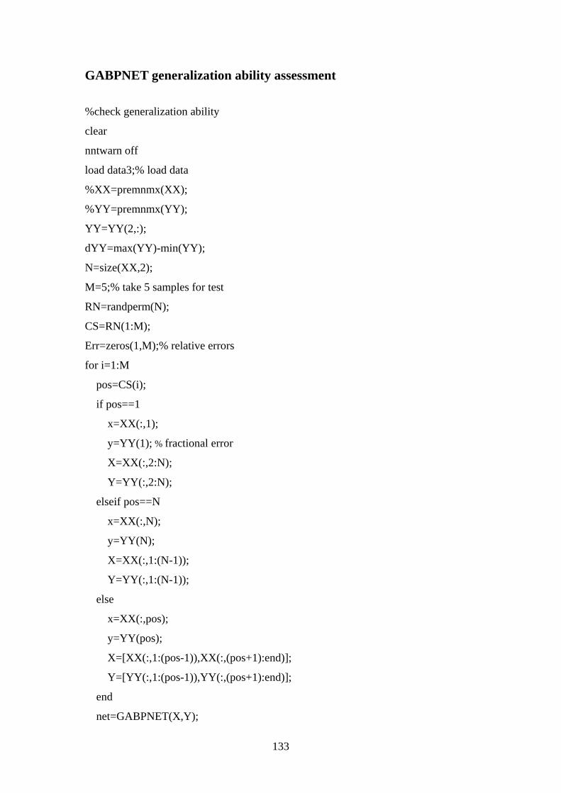
133

GABPNET generalization ability assessment

%check generalization ability

clear

nntwarn off

load data3;% load data

%XX=premnmx(XX);

%YY=premnmx(YY);

YY=YY(2,:);

dYY=max(YY)-min(YY);

N=size(XX,2);

M=5;% take 5 samples for test

RN=randperm(N);

CS=RN(1:M);

Err=zeros(1,M);% relative errors

for i=1:M

pos=CS(i);

if pos==1

x=XX(:,1);

y=YY(1); % fractional error

X=XX(:,2:N);

Y=YY(:,2:N);

elseif pos==N

x=XX(:,N);

y=YY(N);

X=XX(:,1:(N-1));

Y=YY(:,1:(N-1));

else

x=XX(:,pos);

y=YY(pos);

X=[XX(:,1:(pos-1)),XX(:,(pos+1):end)];

Y=[YY(:,1:(pos-1)),YY(:,(pos+1):end)];

end

net=GABPNET(X,Y);

134

[xx,minXX,maxXX]=premnmx(XX);

[yy,minYY,maxYY]=premnmx(YY);

x=tramnmx(x,minXX,maxXX);

y=sim(net,x);

y=postmnmx(y,minYY,maxYY);

Err(:,i)=(y-YY(:,pos))./YY(:,pos);

end

sum(abs(Err))/M

figure(3)

hist(abs(Err))

figure(4)

stem(abs(Err))

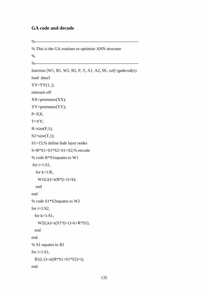
135

GA code and decode

%--------------------------------------------------------------------------

% This is the GA routines to optimize ANN structure

%

%--------------------------------------------------------------------------

function [W1, B1, W2, B2, P, T, A1, A2, SE, val]=gadecod(x)

load data3

YY=YY(1,:);

nntwarn off

XX=premnmx(XX);

YY=premnmx(YY);

P=XX;

T=YY;

R=size(P,1);

S2=size(T,1);

S1=15;% define hide layer nodes

S=R*S1+S1*S2+S1+S2;% encode

% code R*S1equates to W1

for i=1:S1,

for k=1:R,

W1(i,k)=x(R*(i-1)+k);

end

end

% code S1*S2equates to W2

for i=1:S2,

for k=1:S1,

W2(i,k)=x(S1*(i-1)+k+R*S1);

end

end

% S1 equates to B1

for i=1:S1,

B1(i,1)=x((R*S1+S1*S2)+i);

end

136

% S2 equates to B2

for i=1:S2,

B2(i,1)=x((R*S1+S1*S2+S1)+i);

end

% calculate output form S1 and S2

A1=tansig(W1*P,B1);

A2=purelin(W2*A1,B2);

% sum square error

SE=sumsqr(T-A2);

val=1/SE; % fitness

137

Fitness function

function [sol, val] = gabpEval(sol,options)

% val - the fitness of this individual

% sol - the individual, returned to allow for Lamarckian evolution

% options - [current_generation]

load data3

YY=YY(1,:);

nntwarn off

XX=premnmx(XX);

YY=premnmx(YY);

P=XX;

T=YY;

R=size(P,1);

S2=size(T,1);

S1=15;% define hide layer nodes

S=R*S1+S1*S2+S1+S2;%encode

for i=1:S,

x(i)=sol(i);

end;

[W1, B1, W2, B2, P, T, A1, A2, SE, val]=gadecod(x);

138

Data mining main

function Parameter=PARA(CF,Velo)

%% character extraction

%% Input parameters

% CF c

% Velo simulated velocity curve

%% Output parameters

% P1 Contact time

% P2 10% above contact time

% P3 50% above contact time

% P4 90% above contact time

% P5 Peak time

% P6 Peak force

% P7 Kurtosis 1：P6/P1

% P8 Kurtosis 2：P6/P2

% P9 Kurtosis 3：P6/P3

% P10 Kurtosis 4：P6/P4

% P11 Kurtosis 5：statistic peak value

% P12 Skewness 1：Integrated Skewness based on P1 and P5

% P13 Skewness 2：Integrated Skewness based on P2 and P4

% P14 Skewness 2：statistic Skewness

% P15 impact speed

% P16 rebound speed

% P17 COR：P16/P15

% P18 average acceleration

% P19 peak acceleration

%% load test data

F=CF(:,2);

Nonzero=find(F>eps);

pos1=Nonzero(1);

139

pos2=Nonzero(end);

F=F(pos1:pos2);

V=Velo(pos1:pos2,2);

T=CF(pos1:pos2,1);

T=T';

F=F';

V=V';

%% Parameter 1：Contact time

P1t1=T(1);

P1t2=T(end);

P1=P1t2-P1t1;

%% Parameter 2：10% above contact time

maxF=max(F);

pos=find(F>=0.1*maxF);

P2t1=T(pos(1));

P2t2=T(pos(end));

P2=P2t2-P2t1;

%% Parameter 3：50% above contact time

pos=find(F>=0.5*maxF);

P3t1=T(pos(1));

P3t2=T(pos(end));

P3=P3t2-P3t1;

%% Parameter 4：90% above contact time

pos=find(F>=0.9*maxF);

P4t1=T(pos(1));

P4t2=T(pos(end));

P4=P4t2-P4t1;

%% Parameter 5：Peak time

140

pos=find(F==maxF);

P5=mean(T(pos));

%% Parameter 6：Peak force

P6=maxF;

%% Parameter 7：Kurtosis 1：P6/P1

P7=P6/P1;

%% Parameter 8：Kurtosis 2：P6/P2

P8=P6/P2;

%% Parameter 9：Kurtosis 3：P6/P3

P9=P6/P3;

%% Parameter 10：Kurtosis 4：P6/P4

P10=P6/P4;

%% Parameter 11：Kurtosis 5：Statistic Kurtosis

P11=kurtosis(F');

%% Parameter 12：Skewness 1：Integrated Skewness based on P1 and P5

pos1=find(T<=P5);

pos2=find(T>P5);

F1=F(pos1);

F2=F(pos2);

P12=sum(F2)/sum(F1);

%% Parameter 13：Skewness 1：Integrated Skewness based on P2 and P4

t3=0.5*(P4t1+P4t2);

pos1=find(T<=P2t1);

pos1=pos1(end);

pos2=find(T>=P2t2);

141

pos2=pos2(1);

pos3=find(T<=t3);

pos3=pos3(end);

pos4=find(T>t3);

pos4=pos4(1);

F1=F(pos1:pos3);

F2=F(pos4:pos2);

P13=sum(F2)/sum(F1);

%% Parameter 14：Skewness 3：statistic Skewness

P14=skewness(F');

%% Parameter 15：Impact speed

P15=V(1);

%% Parameter 16：Rebound speed

P16=V(end);

%% Parameter 17：COR：P16/P15

P17=abs(P16/P15);

%% Parameter 18：average acceleration

P18=abs((P16-P15)/P1);

%% Parameter 19：peak acceleration

pos1=find(T<=P4t1);

pos2=find(T>=P4t2);

pos1=pos1(end);

pos2=pos2(1);

P19=abs((V(pos2)-V(pos1))/(T(pos2)-T(pos1)));

%% Parameters assembly

142

Parameter=[P1,P2,P3,P4,P5,P6,P7,P8,P9,P10,P11,P12,P13,P14,P15,P16,P17,P18,P19

];

143

Parameter reversing through ANN

function [C10,C01,G1,Tau1]=TEST_hypervisco(CF,V1,V2,COR,XX,YY)

%[C10,C01,G1,Tau1]=TEST_hypervisco(CF,40,-18.4,0.4609,XX,YY)

%% use GABP to reverse the material parameters of HYPERVISCO model

%% Input parameters list

% CF test contact force

% V1 impact speed

% V2 rebound speed（negative）

% COR abs(V2/V1)

%% Output parameters list

% C10,C01,G1,Tau1 are material parameters

%% Step 1：load data

F=CF(:,2);

Nonzero=find(F>eps);

pos1=Nonzero(1);

pos2=Nonzero(end);

F=F(pos1:pos2);

T=CF(pos1:pos2,1);

T=T';

F=F';

% Parameter 1：contact time

P1t1=T(1);

P1t2=T(end);

P1=P1t2-P1t1;

% Parameter 2：10% above contact time

maxF=max(F);

pos=find(F>=0.1*maxF);

P2t1=T(pos(1));

P2t2=T(pos(end));

P2=P2t2-P2t1;

144

% Parameter 3：50% above contact time

pos=find(F>=0.5*maxF);

P3t1=T(pos(1));

P3t2=T(pos(end));

P3=P3t2-P3t1;

% Parameter 4：90% above contact time

pos=find(F>=0.9*maxF);

P4t1=T(pos(1));

P4t2=T(pos(end));

P4=P4t2-P4t1;

% Parameter 5：peak time

pos=find(F==maxF);

P5=mean(T(pos));

% Parameter 6：peak force

P6=maxF;

% Parameter 7：Kurtosis 1：P6/P1

P7=P6/P1;

% Parameter 8：Kurtosis 2：P6/P2

P8=P6/P2;

% Parameter 9：Kurtosis 3：P6/P3

P9=P6/P3;

% Parameter 10：Kurtosis 4：P6/P4

P10=P6/P4;

% Parameter 11：Kurtosis 5：statistic Kurtosis

P11=kurtosis(F');

% Parameter 12：Skewness 1：Integrated Skewness based on P1 and P5

pos1=find(T<=P5);

pos2=find(T>P5);

F1=F(pos1);

F2=F(pos2);

P12=sum(F2)/sum(F1);

% Parameter 13：Skewness 1：Integrated Skewness based on P2 and P4

145

t3=0.5*(P4t1+P4t2);

pos1=find(T<=P2t1);

pos1=pos1(end);

pos2=find(T>=P2t2);

pos2=pos2(1);

pos3=find(T<=t3);

pos3=pos3(end);

pos4=find(T>t3);

pos4=pos4(1);

F1=F(pos1:pos3);

F2=F(pos4:pos2);

P13=sum(F2)/sum(F1);

% Parameter 14：Skewness 3：statistic Skewness

P14=skewness(F');

% Parameter 15：impact speed

P15=V1;

% Parameter 16：rebound speed

P16=V2;

% Parameter 17：COR：P16/P15

P17=COR;

% Parameter 18：average acceleration

P18=abs((P16-P15)/P1);

x=[P1,P2,P3,P4,P5,P6,P7,P8,P9,P10,P11,P12,P13,P14,P15,P16,P17,P18]';

%% Parameters reversing, five networks work in parallel

net1=GABPNET(XX,YY(1,:));

net2=GABPNET(XX,YY(1,:));

net3=GABPNET(XX,YY(1,:));

net4=GABPNET(XX,YY(1,:));

net5=GABPNET(XX,YY(1,:));

[xx,minXX,maxXX]=premnmx(XX);

[yy,minYY,maxYY]=premnmx(YY(1,:));

x=tramnmx(x,minXX,maxXX);

146

y1=sim(net1,x);

y2=sim(net2,x);

y3=sim(net3,x);

y4=sim(net4,x);

y5=sim(net5,x);

y=0.2*(y1+y2+y3+y4+y5);

C10=postmnmx(y,minYY,maxYY);

net1=GABPNET(XX,YY(2,:));

net2=GABPNET(XX,YY(2,:));

net3=GABPNET(XX,YY(2,:));

net4=GABPNET(XX,YY(2,:));

net5=GABPNET(XX,YY(2,:));

[xx,minXX,maxXX]=premnmx(XX);

[yy,minYY,maxYY]=premnmx(YY(2,:));

x=tramnmx(x,minXX,maxXX);

y1=sim(net1,x);

y2=sim(net2,x);

y3=sim(net3,x);

y4=sim(net4,x);

y5=sim(net5,x);

y=0.2*(y1+y2+y3+y4+y5);

C01=postmnmx(y,minYY,maxYY);

net1=GABPNET(XX,YY(3,:));

net2=GABPNET(XX,YY(3,:));

net3=GABPNET(XX,YY(3,:));

net4=GABPNET(XX,YY(3,:));

net5=GABPNET(XX,YY(3,:));

[xx,minXX,maxXX]=premnmx(XX);

[yy,minYY,maxYY]=premnmx(YY(3,:));

x=tramnmx(x,minXX,maxXX);

y1=sim(net1,x);

y2=sim(net2,x);

147

y3=sim(net3,x);

y4=sim(net4,x);

y5=sim(net5,x);

y=0.2*(y1+y2+y3+y4+y5);

G1=postmnmx(y,minYY,maxYY);

net1=GABPNET(XX,YY(4,:));

net2=GABPNET(XX,YY(4,:));

net3=GABPNET(XX,YY(4,:));

net4=GABPNET(XX,YY(4,:));

net5=GABPNET(XX,YY(4,:));

[xx,minXX,maxXX]=premnmx(XX);

[yy,minYY,maxYY]=premnmx(YY(4,:));

x=tramnmx(x,minXX,maxXX);

y1=sim(net1,x);

y2=sim(net2,x);

y3=sim(net3,x);

y4=sim(net4,x);

y5=sim(net5,x);

y=0.2*(y1+y2+y3+y4+y5);

Tau1=postmnmx(y,minYY,maxYY);

148

FE simulation sample data batch processing

%% batch parsing experimental data

clear

load ID

N=size(ID_Test5,1);

P=zeros(N,19);

%%

for i=1:N

%%

cd('D:\Program Files\MATLAB\R2006a\work');

IDi=ID_Test5(i);

sIDi=num2str(IDi);

if IDi<1000

sIDi=['0',sIDi];

end

str1=['D:\Program

Files\MATLAB\R2006a\work\Test5_summary\DES_0',sIDi,'\Parsing_Script_00000'];

cd(str1);

load CF.dat;

load Velo.dat;

cd('D:\Program Files\MATLAB\R2006a\work');

Parameter=PARA(CF,Velo);

P(i,:)=Parameter;

%%

end

149

ODB file data conversion

from odbAccess import *

odb = openOdb(path='Hypervisco.odb')

step1 = odb.steps['Step-1']

print step1.historyRegions

region1 = step1.historyRegions['Node GROUND-1.5']

region2 = step1.historyRegions['Node SOLIDBALL-1.2']

RTData = region1.historyOutputs['RF3'].data

VData = region2.historyOutputs['V3'].data

CFFile = open('CF.dat','w')

for time, RF3 in RTData :

CFFile.write('%10.4E %10.4E\n' % (time, RF3))

CFFile.close()

VeloFile = open('Velo.dat','w')

for time, V3 in VData :

VeloFile.write('%10.4E %10.4E\n' % (time, V3))

VeloFile.close()

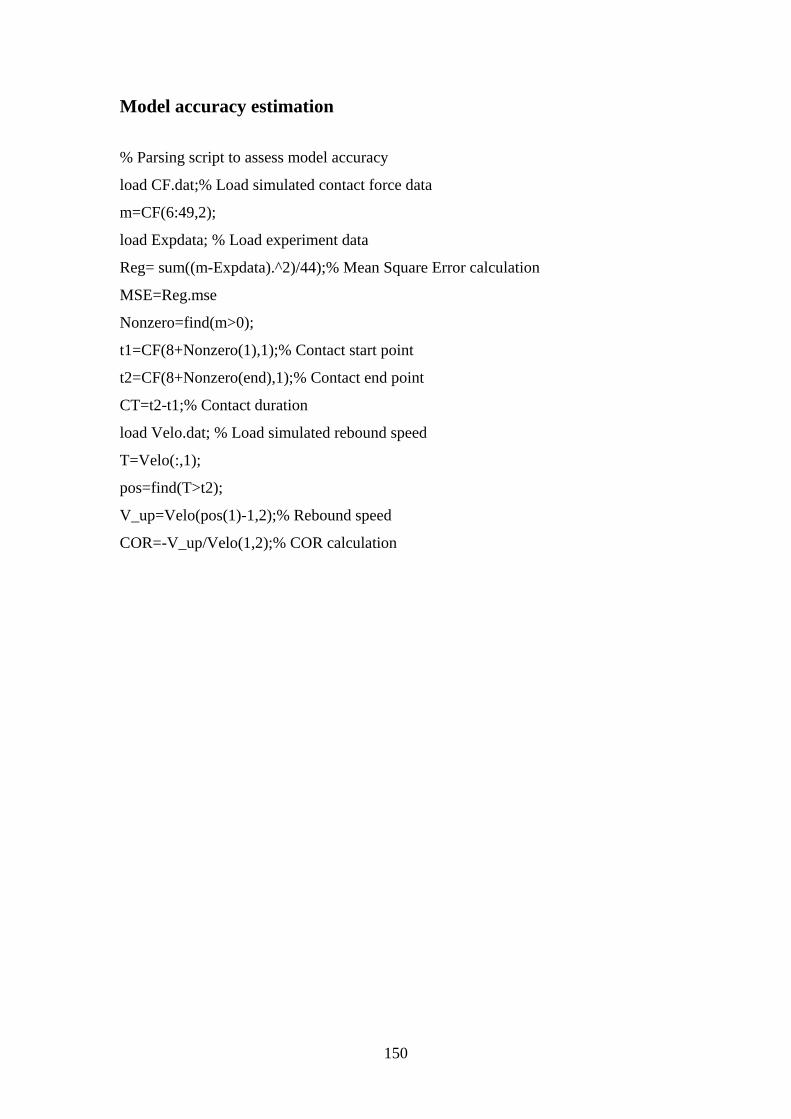
150

Model accuracy estimation

% Parsing script to assess model accuracy

load CF.dat;% Load simulated contact force data

m=CF(6:49,2);

load Expdata; % Load experiment data

Reg= sum((m-Expdata).^2)/44);% Mean Square Error calculation

MSE=Reg.mse

Nonzero=find(m>0);

t1=CF(8+Nonzero(1),1);% Contact start point

t2=CF(8+Nonzero(end),1);% Contact end point

CT=t2-t1;% Contact duration

load Velo.dat; % Load simulated rebound speed

T=Velo(:,1);

pos=find(T>t2);

V_up=Velo(pos(1)-1,2);% Rebound speed

COR=-V_up/Velo(1,2);% COR calculation

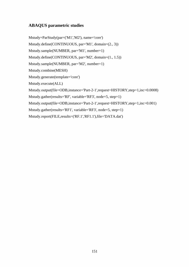
151

ABAQUS parametric studies

Mstudy=ParStudy(par=('M1','M2'), name='core')

Mstudy.define(CONTINUOUS, par='M1', domain=(2., 3))

Mstudy.sample(NUMBER, par='M1', number=1)

Mstudy.define(CONTINUOUS, par='M2', domain=(1., 1.5))

Mstudy.sample(NUMBER, par='M2', number=1)

Mstudy.combine(MESH)

Mstudy.generate(template='core')

Mstudy.execute(ALL)

Mstudy.output(file=ODB,instance='Part-2-1',request=HISTORY,step=1,inc=0.0008)

Mstudy.gather(results='RF', variable='RF3', node=5, step=1)

Mstudy.output(file=ODB,instance='Part-2-1',request=HISTORY,step=1,inc=0.001)

Mstudy.gather(results='RF1', variable='RF3', node=5, step=1)

Mstudy.report(FILE,results=('RF.1','RF1.1'),file='DATA.dat')