Embed Size (px)
Citation preview

Development of a Queue Warning System Utilizing ATM Infrastructure System Development and Field Testing
John Hourdos, Principal InvestigatorMinnesota Traffic Observatory Deparment of Civil, Environmental, and Geo-EngineeringUniversity of Minnesota
June 2017
Research ProjectFinal Report 2017-20
• mndot.gov/research

To request this document in an alternative format, such as braille or large print, call 651-366-4718 or 1-800-657-3774 (Greater Minnesota) or email your request to [email protected]. Pleaserequest at least one week in advance.
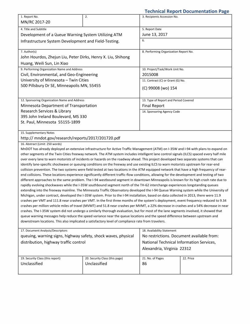
Technical Report Documentation Page 1. Report No. 2. 3. Recipients Accession No.
MN/RC 2017-20
4. Title and Subtitle 5. Report Date
Development of a Queue Warning System Utilizing ATM June 13, 2017
Infrastructure System Development and Field-Testing. 6.
7. Author(s)
John Hourdos, Zhejun Liu, Peter Dirks, Henry X. Liu, Shihong
Huang, Weili Sun, Lin Xiao
8. Performing Organization Report No.
9. Performing Organization Name and Address 10. Project/Task/Work Unit No.
Civil, Environmental, and Geo-Engineering University of Minnesota – Twin Cities 500 Pillsbury Dr SE, Minneapolis MN, 55455
2015008 11. Contract (C) or Grant (G) No.
(C) 99008 (wo) 154
13. Type of Report and Period Covered12. Sponsoring Organization Name and Address
Minnesota Department of Transportation Research Services & Library 395 John Ireland Boulevard, MS 330 St. Paul, Minnesota 55155-1899
Final Report 14. Sponsoring Agency Code
15. Supplementary Notes
http:// mndot.gov/research/reports/2017/201720.pdf 16. Abstract (Limit: 250 words)
MnDOT has already deployed an extensive infrastructure for Active Traffic Management (ATM) on I-35W and I-94 with plans to expand on
other segments of the Twin Cities freeway network. The ATM system includes intelligent lane control signals (ILCS) spaced every half mile
over every lane to warn motorists of incidents or hazards on the roadway ahead. This project developed two separate systems that can
identify lane-specific shockwave or queuing conditions on the freeway and use existing ILCS to warn motorists upstream for rear-end
collision prevention. The two systems were field tested at two locations in the ATM equipped network that have a high frequency of rear-
end collisions. These locations experience significantly different traffic-flow conditions, allowing for the development and testing of two
different approaches to the same problem. The I-94 westbound segment in downtown Minneapolis is known for its high crash rate due to
rapidly evolving shockwaves while the I-35W southbound segment north of the TH-62 interchange experiences longstanding queues
extending into the freeway mainline. The Minnesota Traffic Observatory developed the I-94 Queue Warning system while the University of
Michigan, under contract, developed the I-35W system. Prior to the I-94 installation, based on data collected in 2013, there were 11.9
crashes per VMT and 111.8 near crashes per VMT. In the first three months of the system’s deployment, event frequency reduced to 9.34
crashes per million vehicle miles of travel (MVMT) and 51.8 near crashes per MVMT, a 22% decrease in crashes and a 54% decrease in near
crashes. The I-35W system did not undergo a similarly thorough evaluation, but for most of the lane segments involved, it showed that
queue warning messages help reduce the speed variance near the queue locations and the speed difference between upstream and
downstream locations. This also implicated a satisfactory level of compliance rate from travelers.
17. Document Analysis/Descriptors 18. Availability Statement
queuing, warning signs, highway safety, shock waves, physical
distribution, highway traffic control
No restrictions. Document available from:
National Technical Information Services,
Alexandria, Virginia 22312
19. Security Class (this report) 20. Security Class (this page) 21. No. of Pages 22. Price
Unclassified Unclassified 86
Development of a Queue Warning System Utilizing
ATM Infrastructure System Development and Field Testing.
FINAL REPORT
Prepared by:
John Hourdos
Zhejun Liu
Peter Dirks
Minnesota Traffic Observatory
Department of Civil, Environmental, and Geo-Engineering
University of Minnesota
Henry X. Liu
Shihong Huang
Weili Sun
Lin Xiao
Department of Civil and Environmental Engineering
University of Michigan
June 2017
Published by:
Minnesota Department of Transportation
Research Services & Library
395 John Ireland Boulevard, MS 330
St. Paul, Minnesota 55155-1899
This report represents the results of research conducted by the authors and does not necessarily represent the views or policies of the Minnesota Department of Transportation or the Minnesota Traffic Observatory. This report does not contain a standard or specified technique.
The authors, the Minnesota Department of Transportation, and Minnesota Traffic Observatory do not endorse products or manufacturers. Trade or manufacturers’ names appear herein solely because they are considered essential to this report because they are considered essential to this report. Dr. Henry Liu and the University of Minnesota have equity and royalty interests in SMART Signal Technologies, Inc., a Minnesota-based private company which could commercially benefit from the results of the research described in Chapter 3 These relationships have been reviewed and managed by the University of Minnesota in accordance with its Conflict of Interests policies.

ACKNOWLEDGMENTS
This work was supported by the Minnesota Department of Transportation (MnDOT). The authors would
like to thank Brian Kary, Jesse Larson and Douglas Lau of MnDOT for their assistance in this project. The
authors would also like to thank Gordon Parikh and Derek Lehrke at the Minnesota Traffic Observatory
University of Minnesota for helping to record video data and maintaining the data collection
infrastructure. The research team would also like to acknowledge the support this project has received
from the Roadway Safety Institute, the University Transportation Center for USDOT Region 5 under the
Moving Ahead for Progress in the 21st Century Act (MAP-21) federal transportation bill passed in 2012.
TABLE OF CONTENTS
Introduction ....................................................................................................................1
Development and Field Deployment of a Queue Warning System on I-94 WB Based on
Detection of Crash-Prone Conditions ..................................................................................................4
2.1 Study Site and Available Data ............................................................................................................. 4
2.2 Traffic Measurements and Metrics .................................................................................................... 7
2.2.1 Temporal Metrics ........................................................................................................................ 8
2.2.2 Spatial Metrics ............................................................................................................................. 8
2.2.3 Heuristic Metrics ....................................................................................................................... 11
2.2.4 Individual Vehicle Speed Noise Reduction ................................................................................ 12
2.3 Crash Probability Model ................................................................................................................... 12
2.3.1 System Architecture .................................................................................................................. 12
2.3.2 Control Algorithm ...................................................................................................................... 13
2.3.3 Control Logic .............................................................................................................................. 15
2.3.4 External Controls ....................................................................................................................... 17
2.3.5 Interface and Control Station .................................................................................................... 17
2.4 System Calibration and Validation.................................................................................................... 19
2.4.1 Calibration Basics ...................................................................................................................... 19
2.5 Historical Incident Likelihood Score ................................................................................................. 21
2.5.1 Representation of Traffic Condition .......................................................................................... 21
2.5.2 Data Normalization ................................................................................................................... 21
2.5.3 Similarity .................................................................................................................................... 22
2.5.4 Modeling Crash Likelihood ........................................................................................................ 22
2.5.5 Alarm Efficiency Score ............................................................................................................... 23
2.6 Results and Discussion ...................................................................................................................... 24
2.6.1 Detection Rates ......................................................................................................................... 25
2.6.2 System False Alarm Rate ........................................................................................................... 27
2.6.3 System Limitations .................................................................................................................... 28
2.7 Conclusions ....................................................................................................................................... 28
Development and Field Deployment of a Queue Warning System on I-35W SB Based on
Freeway Queue Length Estimation ................................................................................................... 30
3.1 Project Motivation ............................................................................................................................ 30
3.2 Project Objectives ............................................................................................................................. 30
3.3 Literature Review.............................................................................................................................. 30
3.3.1 Literature Review on Freeway Queue Length Estimation ......................................................... 30
3.3.2 Literature Review on Intelligent Lane Crash Signal ................................................................... 33
3.4 Data Collection Device Installation and Data Description ................................................................ 35
3.4.1 Implementation Location .......................................................................................................... 35
3.4.2 Detector Pin Assignment ........................................................................................................... 37
3.4.3 Data Description ........................................................................................................................ 40
3.5 Algorithm Development (I-35W Test Site) ....................................................................................... 41
3.5.1 Online Queue Length Estimation Algorithm ............................................................................. 41
3.5.2 Field Test of Queue Estimation Algorithm ................................................................................ 48
3.5.3 Algorithm of Triggering Queue Warning Messages .................................................................. 52
3.6 System Deployment and Evaluation ................................................................................................. 52
3.6.1 Queue Warning System Development ...................................................................................... 53
3.7 Discussion ......................................................................................................................................... 66
Concluding Remarks ...................................................................................................... 67
REFERENCES .................................................................................................................................... 68
LIST OF FIGURES
Figure 2.1 Aerial view of implementation site. ............................................................................................. 5
Figure 2.2 Machine Vision Sensors ............................................................................................................... 6
Figure 2.3 System Architecture ................................................................................................................... 14
Figure 2.4 MnDOT changeable message boards with warning displayed. ................................................. 16
Figure 2.5 QWARN Monitoring Station at the MTO ................................................................................... 18
Figure 2.6 Detail of the User Interface of the QWARN System .................................................................. 19
Figure 2.7 Crash Likelihood Score for a Target Day .................................................................................... 23
Figure 2.8 Alarm Efficiency Score for Different Sets of Thresholds ............................................................ 24
Figure 3.1 Implementation locations .......................................................................................................... 36
Figure 3.2 Controller cabinet with data collection units ............................................................................ 38
Figure 3.3 A sample of event-based data ................................................................................................... 40
Figure 3.4 Paired and unpaired long occupancy and headway data ......................................................... 42
Figure 3.5 Estimation of density and flow rate ........................................................................................... 44
Figure 3.6 Flowchart of the queue estimation algorithm ........................................................................... 46
Figure 3.7 Merge of jam traffic: (a) without merge; (b) with merge .......................................................... 48
Figure 3.8 Layout of loop detectors on a southbound I-35W segment ...................................................... 49
Figure 3.9 Queue estimation results ........................................................................................................... 50
Figure 3.10 MOEs of the field test: (a) speed; (b) flow rate; (c) density; (d) prediction ability ................. 51
Figure 3.11 The queue warning system displaying warning message ........................................................ 52
Figure 3.12 System structure ...................................................................................................................... 53
Figure 3.13 A snapshot of the developed software .................................................................................... 54
Figure 3.14 Mean value and standard deviation of speed at S12 .............................................................. 58
Figure 3.15 Mean value and standard deviation of speed at S14 .............................................................. 59
Figure 3.16 Mean value and standard deviation of speed on Lane 3 at S14: TH62 direction and I-35W
direction ...................................................................................................................................................... 60
Figure 3.17 Mean speed at S15: further downstream in I-35W direction .................................................. 62
Figure 3.18 Speed difference across Stations S12 and S14 ....................................................................... 63
Figure 3.19 Speed difference across Stations S14 and S1718 ................................................................... 63
Figure 3.20 Mean value and standard deviation of speed in morning peak in I-35W direction ............... 64
Figure 3.21 Mean value and standard deviation of speed in evening peak in TH62 direction ................. 65
LIST OF TABLES
Table 2-1 Summary of data types and purpose ............................................................................................ 6
Table 2-2 Breakdown of system performance in right lane by component ............................................... 25
Table 2-3 Detection rates during the evaluation period ............................................................................ 26
Table 2-4 Event frequencies per million vehicles traveled (VMT) .............................................................. 27
Table 2-5 Average daily volumes during historical and current studies ..................................................... 27
Table 3-1 Implementation locations and network settings ........................................................................ 37
Table 3-2 Detector pin assignment table .................................................................................................... 39
Table 3-3 Hypothesis test (test hypothesis that mean speed at S14 remains the same)........................... 56
EXECUTIVE SUMMARY
In 2014, the Minnesota Department of Public Safety (DPS) reported 15,648 crashes occurred on
Minnesota freeways. These crashes accounted for the death of 38 people and the injury of 5,031 people
(3). Rear-end crashes are a typical type of crash on freeways. Although, rear-end crashes can happen
any time there is a disturbance, research has shown (4) that there are traffic conditions that are
associated with collisions, specifically rear-end collisions. Prior studies have shown that such crash prone
traffic Conditions (CPCs) can be detected over other traffic conditions encountered on freeway traffic.
The research described in this report aimed to develop and field test two queue warning systems using
different philosophies in regard to rear-end collision safety. The first system’s philosophy, follows the
premise that freeway rear-end collisions tend to occur in extended stop-and-go traffic or at end-of-
queue locations (29). Such unconditional queue warning systems usually provide warning messages in
an unselective manner, i.e., react to all the queues based on the assumption that all propagating queues
are dangerous and drivers should be warned. Conditions on I-35W southbound in Minneapolis, MN,
support this hypothesis, and it is there where the first system prototype was developed and deployed.
This system was developed by a research team lead by Dr. Henry Liu at the University of Michigan. The
second queue warning system is based on the hypothesis that not all congestion events are dangerous
but there are certain traffic conditions that are crash prone regardless of whether they result in standing
queues or not. Such CPCs can be isolated, fast moving shockwaves, involving only a small number of
vehicles in the deceleration-stop-acceleration cycle. For such conditions, a much more dense detection
infrastructure is needed. One location where such conditions have been identified and result in more
than 100 crashes per year is the westbound section of I-94 in downtown Minneapolis. In this location,
the Minnesota Traffic Observatory has had a permanent Field Lab since 2002. Based on the framework
proposed by Dr. Hourdos (4), this effort approaches the topic from the quantification of traffic flow to
the multi-layer system design along with different approaches including traffic assessment modeling and
the development of control algorithms. This approach utilizes individual vehicle measurements including
individual vehicle speeds and time headways, as the major type of data for the system operation. The
prototype of a CPC detection-based queue warning system was developed by a research team lead by
Dr. John Hourdos at the University of Minnesota.
I-94 WB Queue Warning System Description and Results
The I-94 CPC Queue Warning system follows a three-layer design. The crash probability layer collects
real-time individual vehicle measurements and processes them to remove noise. The filtered data then
pass to the crash-probability model to assess the likelihood of a crash. This crash likelihood along with
additional traffic information, such as speeds and headways, are passed to the second layer, the
algorithm layer. In this layer, the algorithm decides if a warning message should be generated by
comparing the crash probability with preset thresholds and real-time traffic conditions. A decision of
whether to raise or drop the alarm is being generated and passed to the third layer, system control, in
which requirements from policy makers are applied to modify the result before delivering it to the
message sign in the field. Specifically, as part of the terms for the deployment of the system, two
overrides were included and the preexisting MnDOT signs’ refresh rate was kept. Two sets of Intelligent
Lane Control Signs (ILCSs) are used to communicate the warnings to the drivers. The overrides are
intended to limit possible overexposure of drivers to the warning by what was, at the time of
implementation, an unproven system and consist of a time override and a congestion override. The time
override prevents the sign from being turned on, regardless of the alarm status before noon or after 8
p.m. The congestion override also prevents the sign from being turned on when five consecutive 30-
second average speed measurements at the loop detector near the farthest upstream sign are below 25
mph. This override is intended to reduce driver overexposure to the warning by not displaying a warning
when drivers are already travelling slowly. The rate at which the sign is updated is a result of the sign
being part of the MnDOT Twin Cities metro-wide network. Initial activation can vary from a few seconds
to one minute, depending on the synchronization between the independent queue warning system and
the traffic operations system that controls the signs. This delay amplifies short gaps in the alarm
activation.
To obtain the ground truth on which the I-94 system was evaluated, event observations were collected
during a three-month evaluation period (from June 2016 to August 2016). This involved manual
reduction of video from multiple cameras recording crashes and near-crashes, as well as the exact times
the sign changed states. Data from 55 weekdays with sufficient video footage in this period were used
to establish ground truth. Some weekdays were excluded due to corrupted video files or equipment
maintenance. Based on the ground truth established, detection rates under different system conditions
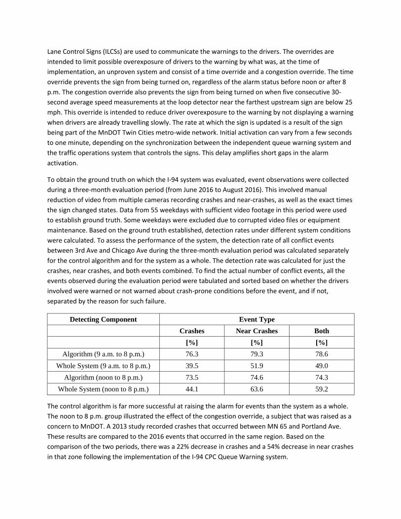
were calculated. To assess the performance of the system, the detection rate of all conflict events
between 3rd Ave and Chicago Ave during the three-month evaluation period was calculated separately
for the control algorithm and for the system as a whole. The detection rate was calculated for just the
crashes, near crashes, and both events combined. To find the actual number of conflict events, all the
events observed during the evaluation period were tabulated and sorted based on whether the drivers
involved were warned or not warned about crash-prone conditions before the event, and if not,
separated by the reason for such failure.
Detecting Component Event Type
Crashes Near Crashes Both
[%] [%] [%]
Algorithm (9 a.m. to 8 p.m.) 76.3 79.3 78.6
Whole System (9 a.m. to 8 p.m.) 39.5 51.9 49.0
Algorithm (noon to 8 p.m.) 73.5 74.6 74.3
Whole System (noon to 8 p.m.) 44.1 63.6 59.2
The control algorithm is far more successful at raising the alarm for events than the system as a whole.
The noon to 8 p.m. group illustrated the effect of the congestion override, a subject that was raised as a
concern to MnDOT. A 2013 study recorded crashes that occurred between MN 65 and Portland Ave.
These results are compared to the 2016 events that occurred in the same region. Based on the
comparison of the two periods, there was a 22% decrease in crashes and a 54% decrease in near crashes
in that zone following the implementation of the I-94 CPC Queue Warning system.
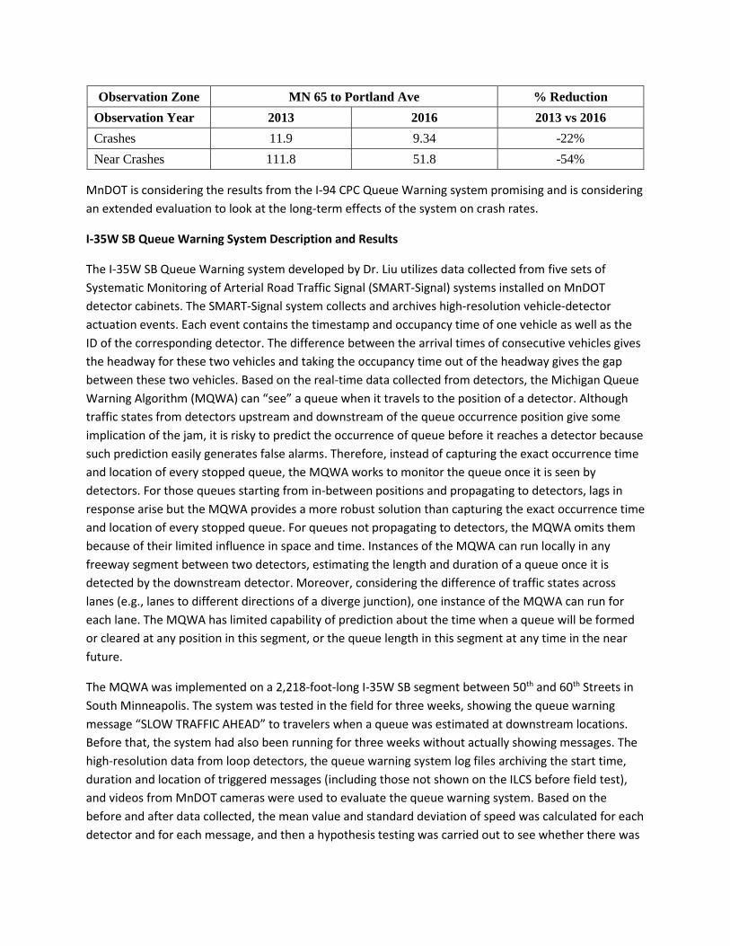
Observation Zone MN 65 to Portland Ave % Reduction
Observation Year 2013 2016 2013 vs 2016
Crashes 11.9 9.34 -22%
Near Crashes 111.8 51.8 -54%
MnDOT is considering the results from the I-94 CPC Queue Warning system promising and is considering
an extended evaluation to look at the long-term effects of the system on crash rates.
I-35W SB Queue Warning System Description and Results
The I-35W SB Queue Warning system developed by Dr. Liu utilizes data collected from five sets of
Systematic Monitoring of Arterial Road Traffic Signal (SMART-Signal) systems installed on MnDOT
detector cabinets. The SMART-Signal system collects and archives high-resolution vehicle-detector
actuation events. Each event contains the timestamp and occupancy time of one vehicle as well as the
ID of the corresponding detector. The difference between the arrival times of consecutive vehicles gives
the headway for these two vehicles and taking the occupancy time out of the headway gives the gap
between these two vehicles. Based on the real-time data collected from detectors, the Michigan Queue
Warning Algorithm (MQWA) can “see” a queue when it travels to the position of a detector. Although
traffic states from detectors upstream and downstream of the queue occurrence position give some
implication of the jam, it is risky to predict the occurrence of queue before it reaches a detector because
such prediction easily generates false alarms. Therefore, instead of capturing the exact occurrence time
and location of every stopped queue, the MQWA works to monitor the queue once it is seen by
detectors. For those queues starting from in-between positions and propagating to detectors, lags in
response arise but the MQWA provides a more robust solution than capturing the exact occurrence time
and location of every stopped queue. For queues not propagating to detectors, the MQWA omits them
because of their limited influence in space and time. Instances of the MQWA can run locally in any
freeway segment between two detectors, estimating the length and duration of a queue once it is
detected by the downstream detector. Moreover, considering the difference of traffic states across
lanes (e.g., lanes to different directions of a diverge junction), one instance of the MQWA can run for
each lane. The MQWA has limited capability of prediction about the time when a queue will be formed
or cleared at any position in this segment, or the queue length in this segment at any time in the near
future.
The MQWA was implemented on a 2,218-foot-long I-35W SB segment between 50th and 60th Streets in
South Minneapolis. The system was tested in the field for three weeks, showing the queue warning
message “SLOW TRAFFIC AHEAD” to travelers when a queue was estimated at downstream locations.
Before that, the system had also been running for three weeks without actually showing messages. The
high-resolution data from loop detectors, the queue warning system log files archiving the start time,
duration and location of triggered messages (including those not shown on the ILCS before field test),
and videos from MnDOT cameras were used to evaluate the queue warning system. Based on the
before and after data collected, the mean value and standard deviation of speed was calculated for each
detector and for each message, and then a hypothesis testing was carried out to see whether there was
a significant change before and after the deployment of the system. Based on this evaluation
methodology the following conclusions were drawn:
1. In general, travelers on I-35W did respond to the queue-warning message “SLOW TRAFFIC AHEAD”
and the traffic conditions with and without messages showed statistically significant differences.
2. The MQWA was able to smooth traffic by reducing the speed variance at downstream locations and
speed difference between upstream and downstream locations, and therefore reduced the risk of
rear-end crash and potentially improved mobility.
3. It took travelers some time from seeing the messages to taking actions such as slowing down their
vehicles. Consequently, queue warning messages had little to do with the traffic conditions near the
ILCS gantry (50th Street) but had an evident impact on the traffic at downstream locations (Diamond
Lake Road).
4. The standard deviation of speed at the bifurcation location was increased when the traffic
condition farther downstream locations on TH-62 was continuously congested. This might be
because the traffic state in this case was more influenced by the downstream congestion rather
than the upstream arrival, which made the queue warning message not very effective.
5. There was no significant difference between the effect of warning message in the morning peak
and that in the evening peak.
At the time of the writing of this report, both queue warning systems were still in operation. Starting in
April 2018, the I-94 WB segment where the CPC Queue Warning system was operating will be under
construction for three years. MnDOT has expressed the desire to implement two instances of the CPC
Queue Warning upstream of the construction zone to alleviate concerns of rear-end collisions generated
from congestion shockwaves due to capacity reduction in the work zone.
1
INTRODUCTION
As the world’s population continues to rise, roadways are utilized to and beyond the limits for which
they were designed. This destabilizes traffic on freeways and produces dangerous driving conditions. In
2014, US officials reported the occurrence of 6.1 million crashes. These crashes injured 2.3 million
people and killed 32,675 people (1). According to the Minnesota Department of Transportation
(MnDOT), the average cost of a single crash is $7,600 when it involves only property damage, $83,000 to
$570,000 when it involves injury, and as high as $10.6 million when the crash is fatal (2). In 2014, the
Minnesota Department of Public Safety (DPS) reported 15,648 crashes occurred on Minnesota freeways.
These crashes accounted for the death of 38 people and the injury of 5,031 people (3). Rear-end crashes
are a typical type of crash that occurs on freeways. Although, rear-end crashes can happen any time
there is a disturbance, research has shown (4) that there are traffic conditions that are associated with
collisions, specifically rear-end collisions. Prior studies have shown that such crash prone traffic
conditions (CPCs) can be detected and differentiated from other freeway traffic conditions encountered.
Discerning what factors influence crash rates and the way in which they do so has been the aim of many
research projects. Qiu and Nixon (5) reviewed the effects of weather on the likelihood of a crash.
Kopelias et al. (6) studied how the combined effects of geometric, operational, and weather factors
influence crash frequencies. Traffic on urban freeways, however, tends to react differently to those
factors. Golob and Recker (7) found that although collision with objects and the crashes of multiple
vehicles are more frequent on wet roads, rear-end crashes are more likely to occur on dry roads with
good visibility. They proposed that these rear-end crashes are highly correlated to large differences in
individual speed like those seen in “stop-and-go” traffic. Such traffic conditions are often referred to as
traffic shockwaves or traffic oscillations. Zheng et al. (8) studied the effects of traffic oscillations on
freeway crashes and found that traffic oscillations and congestion are highly correlated to freeway
crashes.
Various crash-prediction models (9-14) have been developed using the aforementioned factors. In such
models, crash probability is used as a measure of the likelihood of a crash. Significant association has
been shown between crash probability and traffic conditions. Hourdos et al. (4) utilized crash probability
to detect CPCs on a freeway in Minneapolis, MN. While different approaches to apply crash-prediction
models in real-time environments have been proposed (14-16), implementation of such models into
real-time systems is rare.
A common application for dynamic queue warning systems is in work zones where the reduced capacity
of the roadway cannot accommodate normal traffic volumes. Two systems designed for this application
employ several sensors along the road upstream of the construction zone to detect the location of the
upstream end of the queue. The first queue-warning system (17) uses live remote traffic microwave
sensor (RTMS) data from two sensors (one immediately upstream of the work area and one at the end
of the work area) to extrapolate the location of the back of the queue. The location of the back of the
queue is then displayed on a portable changeable message sign (PCMS) at the location of the upstream
2
sensor. The second queue-warning system (18) uses up to eight speed sensors spread out over seven
miles to detect queues. The system warns drivers approaching the work zone of any queues present
through several upstream PCMSs. The Texas Department of Transportation used the eight-sensor
system in a 96-mile project and found it lowered crash rates by as much as 47% when compared to an
estimate of what they would have been had the system not been deployed.
For metropolitan areas where congestion is commonplace, slightly different approaches are often
employed. One system in Houston, TX, (19) uses machine vision detectors (MVDs) to measure the
speeds of vehicles approaching the area in which congestion generally occurs. When the system detects
three consecutive vehicles with speeds lower than 25 mph, lights flash above a warning sign. Pesti et al.
report decreases of 2% to 6% in vehicle conflicts when this queue warning system is in place. Another
queue warning system deployed on a congestion-prone freeway is in Eugene, OR (20). The system
measures freeway occupancy using three side-fire, dual-beam traffic detectors. When the freeway
vehicle occupancy exceeds thresholds established by the Oregon Department of Transportation (ODOT),
warnings are displayed on the Portable Changeable Message Signs (PCMSs) until the occupancy no
longer exceeds the threshold along with a minimum display time of 5 minutes. The system is reported to
have decreased the crash rate by over 35%.
The United States Department of Transportation (USDOT) is currently developing a connected-vehicle
traffic management system called Intelligent Network Flow Optimization (INFLO) that incorporates
queue warning components but it has not been deployed to date (21). The system relies on vehicle-to-
infrastructure communication to share traffic data for the purpose of warning drivers of queues,
harmonizing speed limits, and coordinating cruise control speeds of platooning vehicles. This report
presents the design, specification, implementation and evaluation of two infrastructure-based queue
warning systems that are capable of detecting dangerous traffic conditions, i.e., crash-prone conditions,
on freeways and delivering warning messages to drivers, in order to increase their alertness to these
traffic conditions and ultimately reduce the crash frequency on urban freeways.
The two queue warning systems were developed and field-tested using different philosophies in regard
to rear-end collision safety. The first system’s philosophy, shared by most of the aforementioned
systems, follows the premise that freeway rear-end collisions tend to occur in extended stop-and-go
traffic or at end-of-queue locations (29). Such unconditional queue warning systems usually provide
warning messages in an unselective manner, i.e., react to all the queues based on the assumption that
all propagating queues are dangerous and drivers should be warned. Conditions on I35W southbound in
Minneapolis, MN, support this hypothesis and it is there where the first system prototype was
developed and deployed. This system was developed by a research team at the University of Michigan
lead by Dr Henry Liu and is described in Chapter 3. The second queue warning system is based on the
hypothesis that not all congestion events, forming queues are dangerous but there are certain traffic
conditions that are Crash Prone regardless of whether they result in standing queues or not. Such CPCs
can be isolated, fast-moving shockwaves involving only a small number of vehicles in the deceleration-
stop-acceleration cycle. For such conditions, a much denser detection infrastructure is needed. One
location where such conditions have been identified and result in more than 100 crashes per year is the

3
westbound section of I-94 in downtown Minneapolis, MN. In this location, the Minnesota Traffic
Observatory has had a permanent Field Lab since 2002. Based on the framework proposed by Hourdos
(4), this effort approaches the topic from the quantification of traffic flow to the multi-layer system
design along with different approaches, including the traffic assessment modeling and the development
of control algorithms. This approach utilizes individual vehicle measurements, including individual
vehicle speeds and time headways, as the major type of data for the system operation. A prototype of a
CPC detection based queue warning system was developed by a research team at the University of
Minnesota led by Dr. John Hourdos and is described in Chapter 2 of this report.
4
DEVELOPMENT AND FIELD DEPLOYMENT OF A
QUEUE WARNING SYSTEM ON I-94 WB BASED ON DETECTION
OF CRASH-PRONE CONDITIONS
This report presents the design, specification, implementation, and evaluation of an infrastructure-
based queue warning system (QWARN) that is capable of detecting dangerous traffic conditions, i.e.,
crash-prone conditions (CPCs), on freeways and delivering warning messages to drivers to increase their
alertness in these traffic conditions and ultimately reduce the crash frequency on urban freeways. This
effort approaches the topic from the quantification of traffic flow to the multi-layer system design along
with different approaches including the traffic assessment modeling and the development of control
algorithms. This report presents the QWARN system architecture and deployment and introduces a new
approach to evaluating efficiency the proposed system that is not bound by the constraints of traditional
evaluation indexes such as false alarm rate. This study utilizes measurements of individual vehicle
speeds and time headways at two fixed locations on the freeway mainline as the main source of data for
the system’s operation. Finally, the report concludes with an evaluation of the proposed system
implemented on a freeway section with a high crash frequency. The queue warning system was
implemented in the right lane of a 1.7-mile-long freeway segment of westbound Interstate 94 (I-94 WB)
near downtown Minneapolis where the event frequency prior to the system’s installation was 11.9
crashes per million vehicles traveled(MVT) and 111.8 near crashes per million vehicles traveled(MVT).
Machine Vision Detectors (MVDs) installed on a nearby rooftop captured the real-time vehicle data. The
data were delivered to a server running the main control algorithm at the Minnesota Traffic Observatory
(MTO) via MTO’s communication network. The control algorithm assesses the “dangerousness” of the
given traffic conditions and responds with a warning result based on a multi-metric traffic evaluation
model and a control-reasoning heuristic.
2.1 STUDY SITE AND AVAILABLE DATA
To best study crashes, conditions must be observed and measured before, during, and shortly after an
actual event. This requirement translates to a need for continuous monitoring and data collection at a
location that maximizes the probability of capturing crashes on camera.
In the Minneapolis-Saint Paul Metropolitan Area (Twin Cities), I-94 connects the two cities and is the
major freeway corridor connecting the two banks of the Mississippi River in the region. The site of this
study is a segment with a length of 1.7 miles on I-94 WB near downtown Minneapolis. This segment of I-
94 is near the exit of I-35W, the west branch of Interstate 35 that runs through Minneapolis. The close
proximity to the downtown area results in a large traffic volume merging in and out these two freeways.
The combination of such a large vehicle volume and great degree of merging often destabilizes traffic on
this freeway segment thereby causing shockwaves where drivers need to reduce their speed in a short
time and space or, when drivers fail to decrease their speed quickly enough, rear-end crashes. According
to MnDOT records, this segment had the highest crash rate in the entire Minnesota freeway system. In
2002, the site exhibited 4.81 crashes per million vehicle miles (MVM) – equivalent to approximately one
5
crash every two days – while the network average is 0.96 crashes per MVM. During the PM peak period,
the aforementioned site exhibited an average of 15.43 crashes/MVM whereas the entire I-94 freeway
experienced only 3.29 crashes/MVM (81)]. Fatalities and severe injuries are very rare since the
prevailing speed during CPCs is relatively low. The majority of crashes result only in property damage.
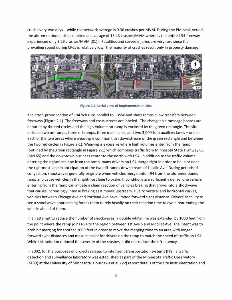
Figure 2.1 Aerial view of implementation site.
The crash-prone section of I-94 WB runs parallel to I-35W and short ramps allow transfers between
freeways (Figure 2.1). The freeways and cross streets are labeled. The changeable message boards are
denoted by the red circles and the high-volume on-ramp is enclosed by the green rectangle. The site
includes two on-ramps, three off-ramps, three main lanes, and two 3,000-foot auxiliary lanes – one in
each of the two areas where weaving is common (just downstream of the green rectangle and between
the two red circles in Figure 2-1). Weaving is excessive where high volumes enter from the ramp
(outlined by the green rectangle in Figure 2-1) which combines traffic from Minnesota State Highway 65
(MN 65) and the downtown business center to the north with I-94. In addition to the traffic volume
entering the rightmost lane from the ramp, many drivers on I-94 merge right in order to be in or near
the rightmost lane in anticipation of the two off-ramps downstream of Lasalle Ave. During periods of
congestion, shockwaves generally originate when vehicles merge onto I-94 from the aforementioned
ramp and cause vehicles in the rightmost lane to brake. If conditions are sufficiently dense, one vehicle
entering from the ramp can initiate a chain reaction of vehicles braking that grows into a shockwave
that causes increasingly intense braking as it moves upstream. Due to vertical and horizontal curves,
vehicles between Chicago Ave and Portland Ave have limited forward sight distance. Drivers’ inability to
see a shockwave approaching forces them to rely heavily on their reaction time to avoid rear-ending the
vehicle ahead of them.
In an attempt to reduce the number of shockwaves, a double white line was extended by 1000 feet from
the point where the ramp joins I-94 to the region between 1st Ave S and Nicollet Ave. The intent was to
prohibit merging for another 1000 feet in order to move the merging zone to an area with longer
forward sight distances and make it easier for drivers on the ramp to match the speed of traffic on I-94.
While this solution reduced the severity of the crashes, it did not reduce their frequency.
In 2002, for the purposes of projects related to intelligent transportation systems (ITS), a traffic
detection and surveillance laboratory was established as part of the Minnesota Traffic Observatory
(MTO) at the University of Minnesota. Hourdakis et al. (22) report details of the site instrumentation and
6
capabilities. Because the site is close to the downtown area, nearby high-rise buildings allowed for the
installation of several cameras and MVDs overlooking the roadway. While most of the sensors are not
utilized by the queue warning system, they provide the means of collecting detailed observations and
determining ground truth.
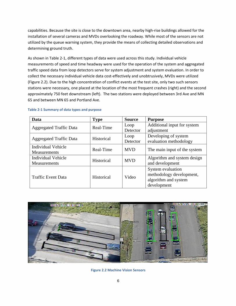
As shown in Table 2-1, different types of data were used across this study. Individual vehicle
measurements of speed and time headway were used for the operation of the system and aggregated
traffic speed data from loop detectors serve for system adjustment and system evaluation. In order to
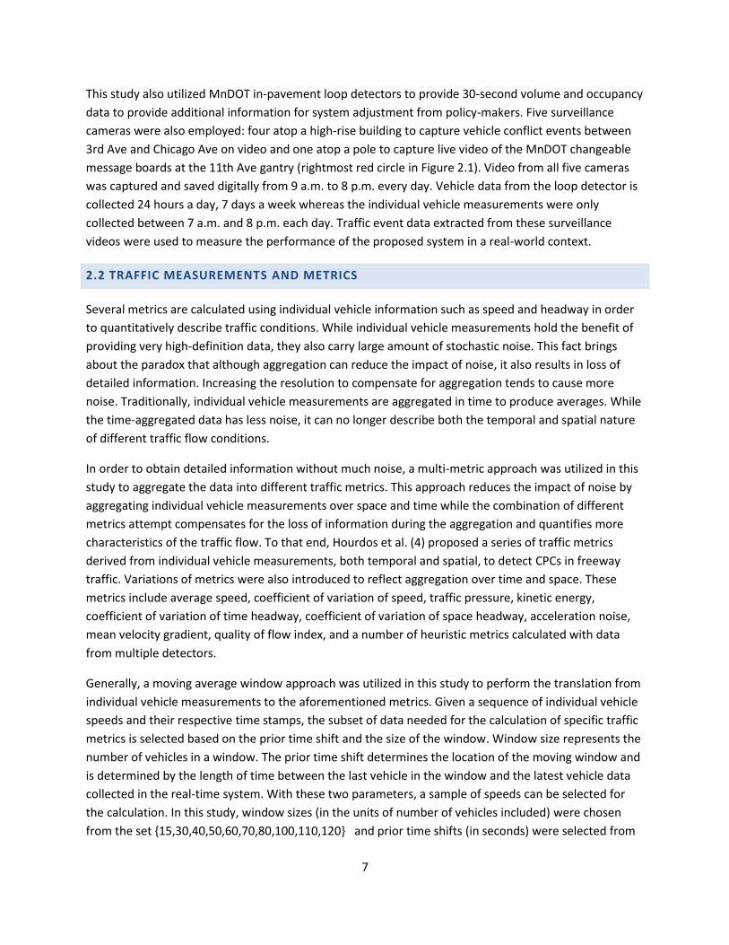
collect the necessary individual vehicle data cost-effectively and unobtrusively, MVDs were utilized
(Figure 2.2). Due to the high concentration of conflict events at the test site, only two such sensors
stations were necessary, one placed at the location of the most frequent crashes (right) and the second
approximately 750 feet downstream (left). The two stations were deployed between 3rd Ave and MN
65 and between MN 65 and Portland Ave.
Table 2-1 Summary of data types and purpose
Data Type Source Purpose
Aggregated Traffic Data Real-Time Loop
Detector
Additional input for system
adjustment
Aggregated Traffic Data Historical Loop
Detector
Developing of system
evaluation methodology
Individual Vehicle
Measurements Real-Time MVD The main input of the system
Individual Vehicle
Measurements Historical MVD
Algorithm and system design
and development
Traffic Event Data Historical Video
System evaluation
methodology development,
algorithm and system
development
Figure 2.2 Machine Vision Sensors
7
This study also utilized MnDOT in-pavement loop detectors to provide 30-second volume and occupancy
data to provide additional information for system adjustment from policy-makers. Five surveillance
cameras were also employed: four atop a high-rise building to capture vehicle conflict events between
3rd Ave and Chicago Ave on video and one atop a pole to capture live video of the MnDOT changeable
message boards at the 11th Ave gantry (rightmost red circle in Figure 2.1). Video from all five cameras
was captured and saved digitally from 9 a.m. to 8 p.m. every day. Vehicle data from the loop detector is
collected 24 hours a day, 7 days a week whereas the individual vehicle measurements were only
collected between 7 a.m. and 8 p.m. each day. Traffic event data extracted from these surveillance
videos were used to measure the performance of the proposed system in a real-world context.
2.2 TRAFFIC MEASUREMENTS AND METRICS
Several metrics are calculated using individual vehicle information such as speed and headway in order
to quantitatively describe traffic conditions. While individual vehicle measurements hold the benefit of
providing very high-definition data, they also carry large amount of stochastic noise. This fact brings
about the paradox that although aggregation can reduce the impact of noise, it also results in loss of
detailed information. Increasing the resolution to compensate for aggregation tends to cause more
noise. Traditionally, individual vehicle measurements are aggregated in time to produce averages. While
the time-aggregated data has less noise, it can no longer describe both the temporal and spatial nature
of different traffic flow conditions.
In order to obtain detailed information without much noise, a multi-metric approach was utilized in this
study to aggregate the data into different traffic metrics. This approach reduces the impact of noise by
aggregating individual vehicle measurements over space and time while the combination of different
metrics attempt compensates for the loss of information during the aggregation and quantifies more
characteristics of the traffic flow. To that end, Hourdos et al. (4) proposed a series of traffic metrics
derived from individual vehicle measurements, both temporal and spatial, to detect CPCs in freeway
traffic. Variations of metrics were also introduced to reflect aggregation over time and space. These
metrics include average speed, coefficient of variation of speed, traffic pressure, kinetic energy,
coefficient of variation of time headway, coefficient of variation of space headway, acceleration noise,
mean velocity gradient, quality of flow index, and a number of heuristic metrics calculated with data
from multiple detectors.
Generally, a moving average window approach was utilized in this study to perform the translation from
individual vehicle measurements to the aforementioned metrics. Given a sequence of individual vehicle
speeds and their respective time stamps, the subset of data needed for the calculation of specific traffic
metrics is selected based on the prior time shift and the size of the window. Window size represents the
number of vehicles in a window. The prior time shift determines the location of the moving window and
is determined by the length of time between the last vehicle in the window and the latest vehicle data
collected in the real-time system. With these two parameters, a sample of speeds can be selected for
the calculation. In this study, window sizes (in the units of number of vehicles included) were chosen
from the set {15,30,40,50,60,70,80,100,110,120} and prior time shifts (in seconds) were selected from
8
the set {10,30,60,120,180,240,300}. The variations in temporal and spatial metrics that follow will be
denoted in the form Metric-Location-Lane-Window_size-Window_end_time. For example, AvgSp-Down-
R-15-30 denotes the average speed among 15 vehicles on the right lane of the downstream station at
least 30 seconds ago.
2.2.1 Temporal Metrics
The following are the definitions of a few of the metrics used in the estimation of the crash probability.
2.2.1.1 Average Speed
Average speed is a common and informative statistic and helps reduce stochastic noise.
2.2.1.2 Coefficient of Variation of Speed (CVS)
In addition to averaging, standard deviation is also a popular way to account for data dispersion. The
coefficient of variation, also called relative standard deviation, standardizes the actual standard
deviation by its sample mean. The CVS is the product of the standard deviation and the mean value of
the speed. As its definition implies, a higher value of the coefficient of variation of speed means higher
variability in the speed data.
2.2.1.3 Coefficient of Variation of Time Headway (CVTH)
The time headway (TH) between vehicles is an important metric that describes safety and level of
service. TH calculation requires individual vehicle arrival times at a point and is simply the difference
between the arrival times of two successive vehicles. For the purposes of this research, the actual time
headways are not as important as the magnitudes and rates of their change, so the chosen metric is the
coefficient of variation of TH in a group of n vehicles.
2.2.2 Spatial Metrics
2.2.2.1 Density
Density (k) is defined as the number of vehicles per unit length of road. It is an important characteristic
of traffic flow in many models describing its relationship with speed. There are several different models
that measure density such as a linear model by Greenshields, a log model by Greenberg, an exponential
model by Underwood, and many others. In this report, density is not used directly but rather as a
component in the calculations of other traffic metrics such as traffic pressure and kinetic energy.
2.2.2.2 Acceleration Noise
Acceleration noise is a measure of the smoothness of the traffic flow based on an estimation of
individual acceleration dispersion. Three factors are highly related to the value of acceleration noise:

9
driver behavior, road conditions and geometry, and traffic conditions. The calculation of the
acceleration noise in this study follows the approximation proposed by Jones and Potts (23).
2.2.2.3 Mean Velocity Gradient
In order to differentiate between different traffic conditions with similar acceleration noise, such as
slow, congested traffic versus fast traffic inside a shockwave, Helly and Baker (24) proposed another
measurement, the mean velocity gradient, described by Equation 2.1.
1
( )
( )
N
i
i
ii
i
MVG
MVGN
ANMVG
u
(2.1)
Where
:MVG Average Mean Velocity Gradient
:iMVG Mean Velocity Gradient of vehicle i
:N The total number of vehicles in a hypothetical mile
( ) :iAN Acceleration Noise
:iu Average speed (mean velocity) of vehicle i
2.2.2.4 Quality of Flow Index
The quality of flow index proposed by Greenshields (25) provides a quantitative metric to describe the
safety of the traffic conditions on a given road based on the number of speed changes and their
frequency (Equation 2.2).

10
1
N
i
i
i
QFI
QFIN
kuQFI f
u
(2.2)
Where
:QFI Average Quality of Flow Index
:iQFI Quality of Flow Index of Vehicle i
:N Total number of vehicles in a hypothetical mile
:u Average speed
:u Absolute sums of speed changes in a mile
:f Number of speed changes in a mile
:k Constant of 1000 when speed unit is mph and the length of the section is one mile.
2.2.2.5 Traffic Pressure
Traffic pressure (TP) was designed to measure the smoothness of traffic flow. It is defined as the product
of speed variance and density (26) as seen in Equation 2.3a. A higher density is generally associated with
a lower average speed. When both the density and the variance of speed are high, it may indicate a
“stop-and-go” traffic that could be dangerous and crash prone.
2
sTP k (2.3a)
Where
:TP Traffic Pressure
2
s : Speed variance
:k Density
2.2.2.6 Kinetic Energy (KE)
Kinetic Energy is a familiar quantity in the world of physics that represents the energy of a moving
object. This measurement can also be modified to quantify the energy stored in the traffic flow. In the
context of traffic flow, kinetic energy measures the energy in the motion of the traffic stream.

11
Similar to the concept of energy used in physics, the total amount of “energy” in a traffic system cannot
change but can be converted to another form. Drew (27) described the antithesis of kinetic energy as
internal energy or erratic motion due to the road geometry and vehicle interactions that corresponds to
an earlier description of acceleration noise. Please note that the “kinetic energy” in this study is for
traffic flow and is different from the kinetic energy of a moving object, which means it is not dependent
on the mass of vehicles but instead on the density of the traffic stream. The formulation of KE is
described in equation 2.3b.
2( )KE ak u (2.3b)
Where
:a kinetic energy correction parameter, a dimensionless constant, here it is taken as 1
:k density of the traffic stream
:u average speed of the stream
2.2.3 Heuristic Metrics
2.2.3.1 Up/Down Speed Difference
The up/down speed difference is the difference between the maximum vehicle speed at the upstream
sensor and the minimum vehicle speed at the downstream sensor. Its purpose is to measure the travel
behavior of a shockwave. For example, when traffic is smooth without shockwaves, the up/down speed
difference should be small. When a shockwave has reached the downstream sensor, but has not yet
reached the upstream sensor, there should be a lower speed downstream than upstream thus resulting
in a high up/down speed difference. A positive up/down speed difference indicates that the maximum
speed of upstream is higher than the minimum speed of downstream. On the other hand, a negative
sign of up/down speed difference indicates that the maximum speed of upstream is lower than the
minimum speed of downstream. The latter case may happen when upstream is congested and
downstream traffic is already recovering from congestion.
2.2.3.2 Right/Middle Lane Speed Difference
As the name suggests, this metric is the difference in speeds between the right lane and the middle lane.
When the traffic on the right lane is significantly slower than that on the middle lane, lane changes
become more dangerous as they require drivers to divert their attention from the traffic ahead and
search for a gap in their mirrors. This increases their reaction time which can be dangerous when
shockwaves approach.
2.2.3.3 Max/Min Speed Difference
This metric measures difference between the maximum speed and minimum speed on a sensor location
for a given prior time shift and window size. When a shockwave hits a location, in a relatively short
12
number of vehicles, the speeds tend to fluctuate and drop and results in a high Max/Min Speed
Difference. Such high value is usually observed in the occurrence of traffic oscillations and crashes.
2.2.4 Individual Vehicle Speed Noise Reduction
All sensors inherently have error and noise in their measurements, and such noise can cause surges in
the crash-likelihood calculation and compromise the accuracy of the model. In order to reduce the noise
in a time series, filtering techniques such as the one proposed by Hourdos (28) in his development of a
crash probability model are often employed. To perform a time series analysis and noise removal, the
original unstructured speed data needs to be translated into a 1-second-speed time series using
interpolation. Two different interpolation methods, linear interpolation and spline interpolation, were
considered as candidates and tested in a preliminary study by the authors. Linear interpolation consists
of simply connecting the data points with straight lines while spline interpolation uses a single,
continuous curve to connect all the points. When comparing these two methods, spline interpolation
was found to be problematic as the requirement that the data points be connected with a smooth curve
produced interpolated speeds that were well outside of the normal range thereby introducing additional
error and noise. Because of this issue with the spline interpolation method, linear interpolation was
selected for this study. Of the several different filters that Hourdos designed and tested on their ability
to remove impulse noise, his Digital FIR Hamming filter was selected to perform the noise reduction for
the system.
After filtering, the data become another time series with lower noise. Given that the time headways
between vehicles are as informative as their speeds, the dataset needs to be returned to its original
form before the traffic metrics are calculated. A reverse interpolation method finding the filtered speeds
at the times of the original data points is implemented.
2.3 CRASH PROBABILITY MODEL
Using the described metrics and their variants as well as the selected digital filter, a crash probability
model was produced. The model is based on a fitted logistic regression model. The model described by
Hourdos (28) was employed to determine the likelihood of a crash which is the main input in both the
CPC detection algorithm and resulting queue warning system.
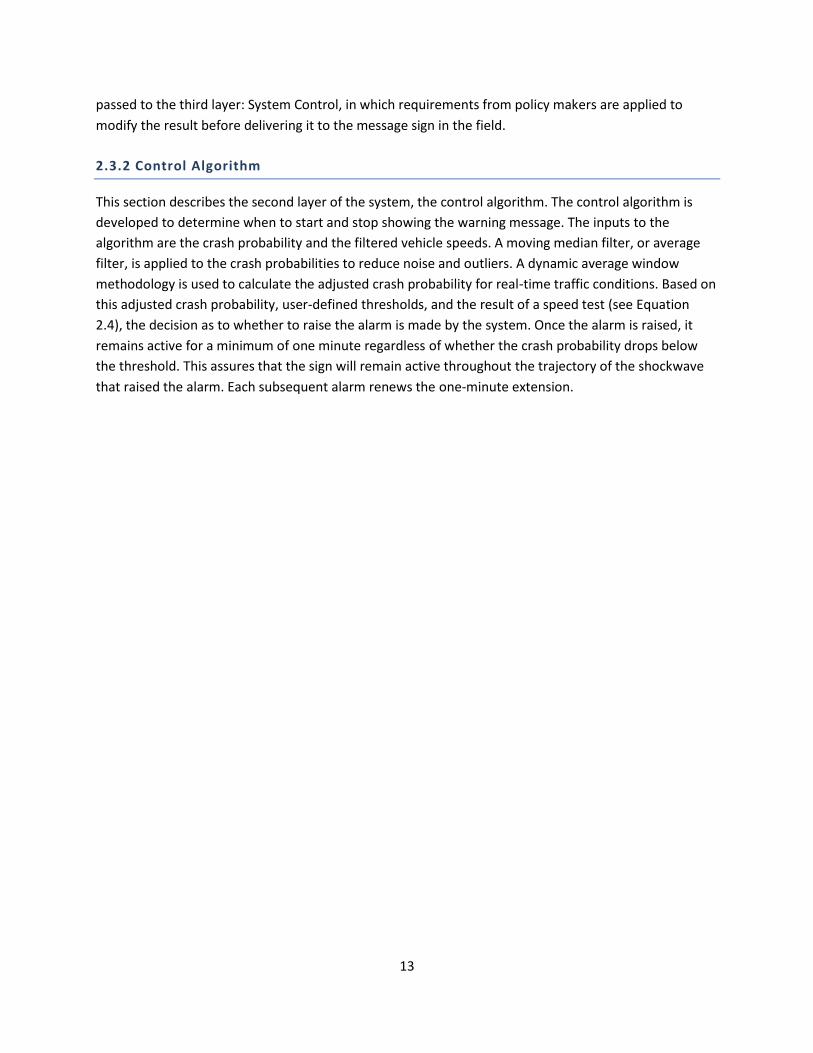
2.3.1 System Architecture
This section presents the system architecture. As shown in Figure 2.3, the system follows a three-layer
design. The Crash Probability layer collects real-time individual vehicle measurements and processes
them to remove noise. The filtered data then pass to the crash-probability model to assess the
likelihood of a crash. This crash likelihood along with additional traffic information such as speeds and
headways are passed to the second layer, the Algorithm layer. In this layer, the algorithm decides if a
warning message should be generated by comparing the crash probability with preset thresholds and
real-time traffic conditions. A decision of whether to raise or drop the alarm is being generated and
13
passed to the third layer: System Control, in which requirements from policy makers are applied to
modify the result before delivering it to the message sign in the field.
2.3.2 Control Algorithm
This section describes the second layer of the system, the control algorithm. The control algorithm is
developed to determine when to start and stop showing the warning message. The inputs to the
algorithm are the crash probability and the filtered vehicle speeds. A moving median filter, or average
filter, is applied to the crash probabilities to reduce noise and outliers. A dynamic average window
methodology is used to calculate the adjusted crash probability for real-time traffic conditions. Based on
this adjusted crash probability, user-defined thresholds, and the result of a speed test (see Equation
2.4), the decision as to whether to raise the alarm is made by the system. Once the alarm is raised, it
remains active for a minimum of one minute regardless of whether the crash probability drops below
the threshold. This assures that the sign will remain active throughout the trajectory of the shockwave
that raised the alarm. Each subsequent alarm renews the one-minute extension.
14
Figure 2.3 System Architecture

15
2.3.3 Control Logic
The crash likelihood alone is not sufficient for determining the precise time to warn the drivers while still
producing consistent and stable decisions. Since the crash probability is a continuous variable, a two-
threshold approach is employed to determine whether a crash likelihood indicates crash-prone
conditions. One threshold for determining the raising of the alarm and a second for determining its
termination. In addition to the crash probability, the algorithm proposed in this report also takes
additional traffic measurements into consideration to increase the accuracy and efficiency of the alarm.
Once the alarm is initiated, it will remain active for a minimum time period, currently one minute. Since
the individual vehicle data is inherently noisy and can change very quickly, the single model structure
used to measure the crash probability can generate spikes when it encounters speed outliers. A spike in
noise caused by outliers takes the form of a sudden surge in the value of crash probability and a sudden
drop a very short time after the surge. The values before and after such spike were usually in similar
ranges. Therefore, such a spike may activate the alarm trigger for only several seconds during which the
alarm shouldn’t be raised. Thus, deciding the status of the alarm based only by the alarm trigger can
lead to frequent changing of warning messages. The control logic of the algorithm can be found below in
Equation 2.4.
1
2
1
1
0
0
( , ) ^ ( )
^ ( , , ) ^ ( )
( )
( )
t tb
t
tb
tb
tb
Greater p SpeedTest v AlarmOn
AlarmOn Greater p TimeCheck t AlarmOff
true v uSpeedTest v
false v u
true t t tTimeCheck t
false t t t
(2.4)
Where
1u : test speed, default is 45 mph. (mph)
0t : last time in the past with an alarm trigger (s)
1 : Starting Threshold
2 : Ending Threshold
tbv : Current Downstream Speed (mph)
tp : Adjusted Crash Probability
16
1
1 t
t i
i t n
p pn
1 1
1 2 2 1
2
( , )
( , , )
( )
t t
t t
t t
f p p
n g p p
h p p
(2.5)
As shown in equations 2.4 and 2.5, the algorithm regards the crash probability as one of the inputs
needed to decide whether to raise or lower the alarm. The adjusted crash probability is used instead of
the direct output from the crash probability model. The value n is the size of the dynamic window used
to average the crash probability. Using a dynamic window size makes the algorithm more sensitive to
crash-prone conditions and reduces the probability of false alarms caused by noise in the measurement.
The dynamic window size is calculated through three conditions, as described in Equation 2.5, with
different results depending on which threshold it is nearest. The controlling hypothesis is that the noise
in the crash probability will be higher around the selected thresholds so more samples are used to
calculate the average unless the crash probability suddenly increases to values close to 100% in which
case the averaging window is made much smaller in order to reduce the delay in raising the alarm.
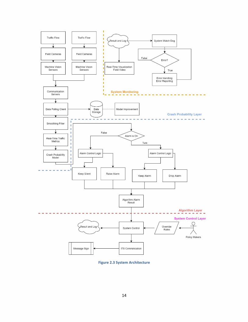
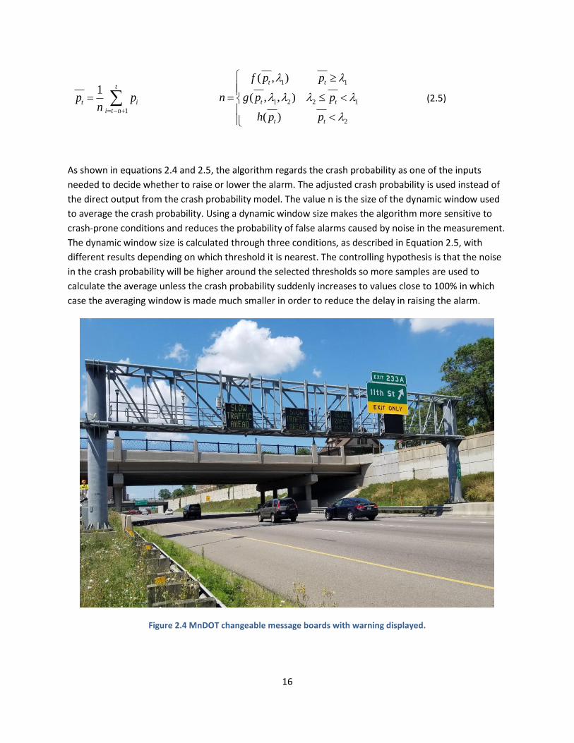
Figure 2.4 MnDOT changeable message boards with warning displayed.
17
2.3.4 External Controls
As part of the terms for the deployment of the system, two overrides were included and the preexisting
MnDOT signs’ (Figure 2.4) refresh rate was kept. The two sets of changeable message boards used are
fixed to gantries above the freeway. The overrides are intended to limit the possibility of overexposure
of drivers to the warning by what was, at the time of implementation, an unproven system and consist
of a time override and a congestion override. The time override prevents the sign from being turned on,
regardless of the alarm status before noon or after 8 p.m. because MnDOT felt that traffic conditions at
those times would be too prone to producing false alarms. The congestion override also prevents the
sign from being turned on when five consecutive 30-second average speed measurements at the loop
detector upstream of the farthest upstream sign are below the MnDOT-imposed threshold of 25 mph.
This override is intended to reduce driver overexposure to the warning by not displaying a warning
when drivers are already travelling slowly. The rate at which the sign is updated is a result of the sign
being part of the MnDOT Twin Cities metro-wide network. Initial activation can vary from a few seconds
to one minute, depending on the synchronization between the independent queue-warning system and
the traffic operations system that controls the signs. This delay amplifies short gaps in the alarm
activation (e.g. even if the alarm is only lowered for 10 seconds, the sign could be off for up to a
minute).
2.3.5 Interface and Control Station
In order to allow the users of QWARN to monitor the system and traffic conditions in real-time, a live
feed of the model result, MVD data, sign status, and cameras used for event detection is available
during the system’s operation. Although the actual application resides in one of the secure servers of
the MTO, a station has been installed in the lab area that allows monitoring of all relevant feeds (Figure
2.5). The QWARN application has been developed to be able to operate from any kind of computer even
in the Cloud. All communications are Ethernet based so any instance of the application that has the right
credentials can poll the MVDs for data and produce the warning messages. At the moment, the
application resides behind the combined firewalls of the University of Minnesota and the MTO.
The system has been developed to include several safety and redundancy features. For example, if for
any reason, the actual application crashes, a separate watchdog application will attempt to restart it
and, if that fails or the entire server is down, an alert email is dispatched to the MTO lab manager
informing him of the situation. The integration with MnDOT’s Regional Traffic Management Center
(RTMC) IRIS traffic operations system is performed through a secure web connection that makes hacking
into either system virtually impossible since IRIS is polling the QWARN application every 30 sec for a
message instead of pushing messages to the traffic operations system. Messages are not dynamically
selectable so even if a hacker could take control of the system the “Slow Traffic Ahead” message is the
only one they would be able to display. Finally, each message IRIS receives has a 45 sec lifetime so if the
warning has been raised and the system crashes the sign will turn off after 45 seconds to avoid cases
where the warnings are still up when conditions are non-crash prone or the congestion override has
been imposed.
18
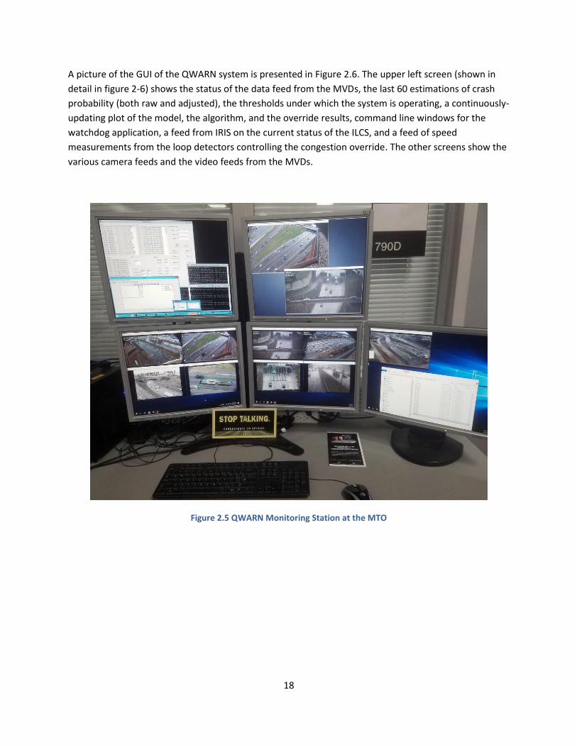
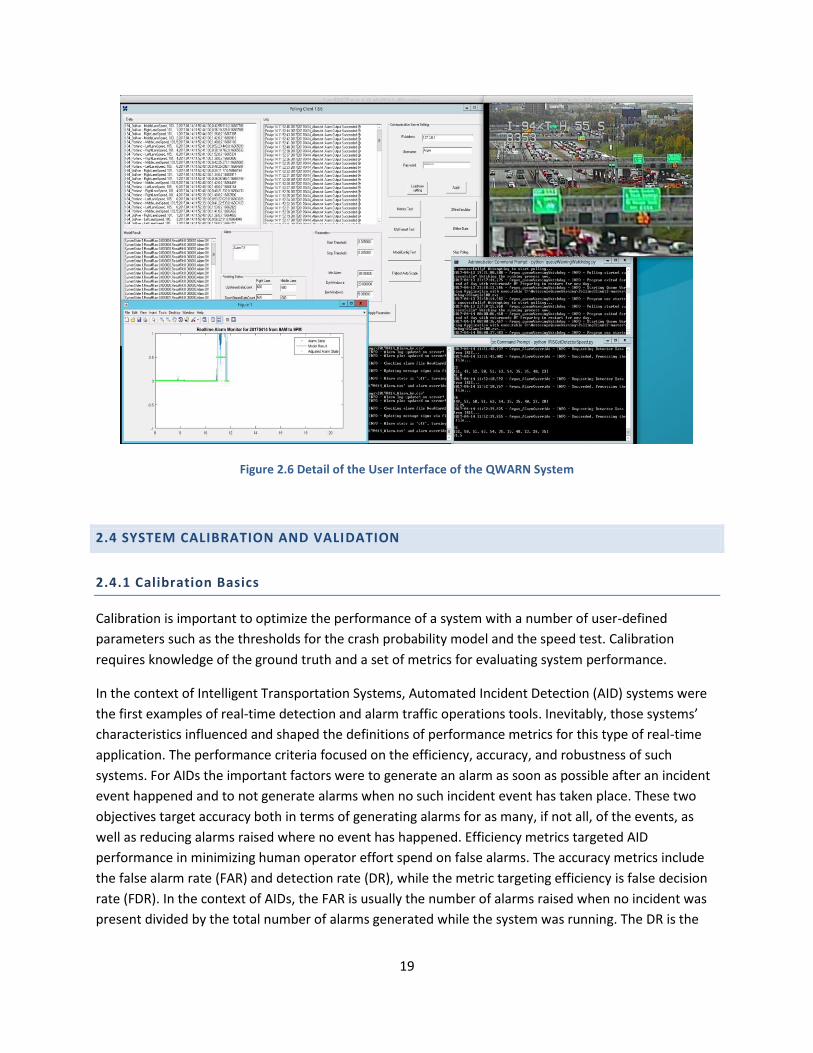
A picture of the GUI of the QWARN system is presented in Figure 2.6. The upper left screen (shown in
detail in figure 2-6) shows the status of the data feed from the MVDs, the last 60 estimations of crash
probability (both raw and adjusted), the thresholds under which the system is operating, a continuously-
updating plot of the model, the algorithm, and the override results, command line windows for the
watchdog application, a feed from IRIS on the current status of the ILCS, and a feed of speed
measurements from the loop detectors controlling the congestion override. The other screens show the
various camera feeds and the video feeds from the MVDs.
Figure 2.5 QWARN Monitoring Station at the MTO
19
Figure 2.6 Detail of the User Interface of the QWARN System
2.4 SYSTEM CALIBRATION AND VALIDATION
2.4.1 Calibration Basics
Calibration is important to optimize the performance of a system with a number of user-defined
parameters such as the thresholds for the crash probability model and the speed test. Calibration
requires knowledge of the ground truth and a set of metrics for evaluating system performance.
In the context of Intelligent Transportation Systems, Automated Incident Detection (AID) systems were
the first examples of real-time detection and alarm traffic operations tools. Inevitably, those systems’
characteristics influenced and shaped the definitions of performance metrics for this type of real-time
application. The performance criteria focused on the efficiency, accuracy, and robustness of such
systems. For AIDs the important factors were to generate an alarm as soon as possible after an incident
event happened and to not generate alarms when no such incident event has taken place. These two
objectives target accuracy both in terms of generating alarms for as many, if not all, of the events, as
well as reducing alarms raised where no event has happened. Efficiency metrics targeted AID
performance in minimizing human operator effort spend on false alarms. The accuracy metrics include
the false alarm rate (FAR) and detection rate (DR), while the metric targeting efficiency is false decision
rate (FDR). In the context of AIDs, the FAR is usually the number of alarms raised when no incident was
present divided by the total number of alarms generated while the system was running. The DR is the
20
number alarms raised when an incident happened divided by the total number of incidents occurred
while the system was in operation. The FDR is the combination of the missed-detection rate and false
alarm rate. Detection systems are required to decide whether to raise the alarm at each time interval
they operate on. FDR is the sum of all intervals that the system raised the alarm for but no incident
existed and the intervals were an incident was present but the system did not raise the alarm, all divided
by the total number of intervals the system was in operation. High DR and low FAR and FDR are
preferred describing an accurate and efficient system. A tradeoff between FAR and DR is a common
issue in such systems. An overly sensitive system may have a very high DR, but by being sensitive, it can
raise the alarm while nothing happened, resulting in a high FAR.
Unfortunately, the aforementioned performance metrics, as defined, are not suitable for the evaluation
of a CPC detection system like the one described in this report. When discussing these metrics, it is
important to note that the objective of AIDs is to detect an event that has happened and alert operators
so they can initiate the process of incident response and clearance. AIDs did not interact with the drivers
and did not aim in changing driving behavior to avoid the event that were designed to detect. The CPC
detection system presented in this report is a crash prevention system which implies the following:
CPC detection systems aim to detect conditions that may lead to a crash but have not done so yet.
Warn drivers that are about to encounter CPCs and help them navigate such unsafe conditions.
Warning the drivers can also change driver behavior enough to eliminate the CPCs themselves.
An AID raising the alarm when no incident happens is a clear failure whereas a CPC detector raising the alarm and nothing bad happening could mean failure if the conditions were not crash prone but it could mean success if a potential crash was avoided.
Incidents are factual events and in extent the detection of their existence is a binary, true or false situation. The causal factors precipitating to a crash, as described in Hourdos et. Al. (4), include the traffic conditions described as crash prone but, more importantly, involve factors related to the individual drivers such as reaction time, awareness, distraction, etc. The same CPCs can result in a crash if a distracted driver is involved or no crash or a near-crash if all drivers involved are attentive.
CPCs are traffic conditions where the probability of a crash is higher than normal, there is no objective way to definitively classify a time period as crash prone where no crash or near-crash has happened.
Using the aforementioned performance metrics as defined to judge the system proposed in this report
can result on overly conservative results and a calibrated system of much lower performance than the
one possible to achieve. Therefore, there is a need for a more robust and leveled performance metric.
Towards that effect, this study proposes a new metric, the Alarm Efficiency Score (AES), that better fits
the nature of a real-time driver warning system. The AES is calculated based on the historical crash
likelihood score and the alarm results of the day on which the system performance is to be evaluated.
Unlike the FAR, the AES is not in a percentage scale. Therefore, in terms of calibration, it only has
meaning when comparing two or multiple results produced by different systems or the same system
with different parameters. A higher AES indicates a better performance.
21
2.5 HISTORICAL INCIDENT LIKELIHOOD SCORE
This study utilized the historical event likelihood approach to measure how dangerous a traffic condition
can be. Given a certain time on a historical day, the similarity of the traffic condition during that time
was compared with the traffic conditions when events happened and calculated a likelihood of an event.
2.5.1 Representation of Traffic Condition
For representing traffic states, two separate ten-dimensional spaces, one of volume and one of
occupancy, were defined. Each traffic condition is represented by a set of these ten-dimensional vectors.
Equation 2.6 is an example of the vector of volume at time t. The value of the 10th dimension equals to
the volume at time t.
9 8 7 6 5 4 3 2 1( ) ( , , , , , , , , , )vol t t t t t t t t t tvec t vol vol vol vol vol vol vol vol vol vol (2.6)
Where
( )volvec t : The volume vector at time t;
tvol : The volume at time t;
t : Time, in this case t is the number of the 30s segment;
The volume and occupancy data from loop detectors were aggregated over 30-second intervals forming
30-second-long time segments. The time variable, t, is equal to the number of the time segment. This
study uses loop detector data for convenience, but individual vehicle measurements can also be used as
long as they are aggregated to represent stable traffic flow over time.
2.5.2 Data Normalization
The natural distributions of volume and occupancy are different. In order to convert them into the same
metric, the data are normalized and representation vectors are created. The normalization function is
described in Equation 2.7. The normalization process involves subtracting the mean from volume data
and then dividing by the standard deviation. The normalization for occupancy is the same as for volume.
1
2
1 1
1
'1 1
( )
n
i i
ii
n n
i i
i i
vol voln
vol
vol voln n
(2.7)
Where
'ivol : Normalized volume for time segment i;
ivol : Original volume for time segment i;
n: Total number of time segment;
22
2.5.3 Similarity
This study uses similarity between a given traffic condition vector and all the condition vectors that
precipitated crashes and near crashes to assess the “dangerousness” of a traffic condition. The
assumption is that if a given traffic condition is very similar to the majority of traffic conditions
corresponding to crashes and near-crashes, the given traffic condition is likely to be dangerous, too.
There are many similarity measurements such as cosine similarity, Euclidean distance, and extended
Jaccard similarity. In this study, different types of similarity metrics were tested. Here, cosine similarity is
chosen to demonstrate the evaluation methodology. Cosine similarity measures the angle of two high-
dimensional vectors to determine their degree of likeness. As shown in Equation 2.8, the nature of
cosine similarity makes it settle in the range (-1,1) with 1 representing the highest similarity.
cos(𝐴, �⃗⃗�) =𝐴∗𝐵
‖𝐴‖‖�⃗⃗�‖ (2.8)
Where A, B are two traffic vectors.
2.5.4 Modeling Crash Likelihood
To evaluate the validity of a model-produced crash likelihood for a given traffic condition, the main
objective is to model the similarity of a given traffic condition compared to those known to be
associated with crashes and near crashes.
Traffic measurements leading up to each historical event were extracted and used to formulate a set of
historical traffic crash-prone conditions. Given a current traffic state represented in the two-vector
approach, the similarity between the historical crash-prone conditions and the current conditions can be
calculated to measure the comprehensive similarity of the two. Based on the assumption that a higher
similarity between a given traffic condition to conditions that resulted in a crash corresponds to a higher
probability of a crash, the likelihood of a crash can be estimated. Extending this concept to each day in
the set of historical days used to evaluate the crash probability model, a map containing the similarity of
each time period to the periods corresponding to historical events (crashes and near-crashes) can be
constructed for each such day.
This map of similarities describes the dangerousness of traffic conditions for each target day. The values
in the map, the crash likelihood score, are produced using Equation 2.9 in which L is the crash likelihood
score, Vd,t, is the volume for traffic condition in day, d ,at time t; Vi,t is the volume of event, i, at time t.
Similarly, O represents the occupancy. This score will be different when the sample of historical crashes
and near crashes is changed. Although it is not a percentage probability, it can quantify the
dangerousness of different traffic conditions in that a higher score denotes more dangerous traffic
conditions as compared to similar conditions that did not result in a crash or near crash. This approach
provides the means to more fairly evaluate the queue warning system even with crash-prone conditions
that may not involve reckless or inattentive drivers. Figure 2.7 shows the values of the crash likelihood
score during a target day.
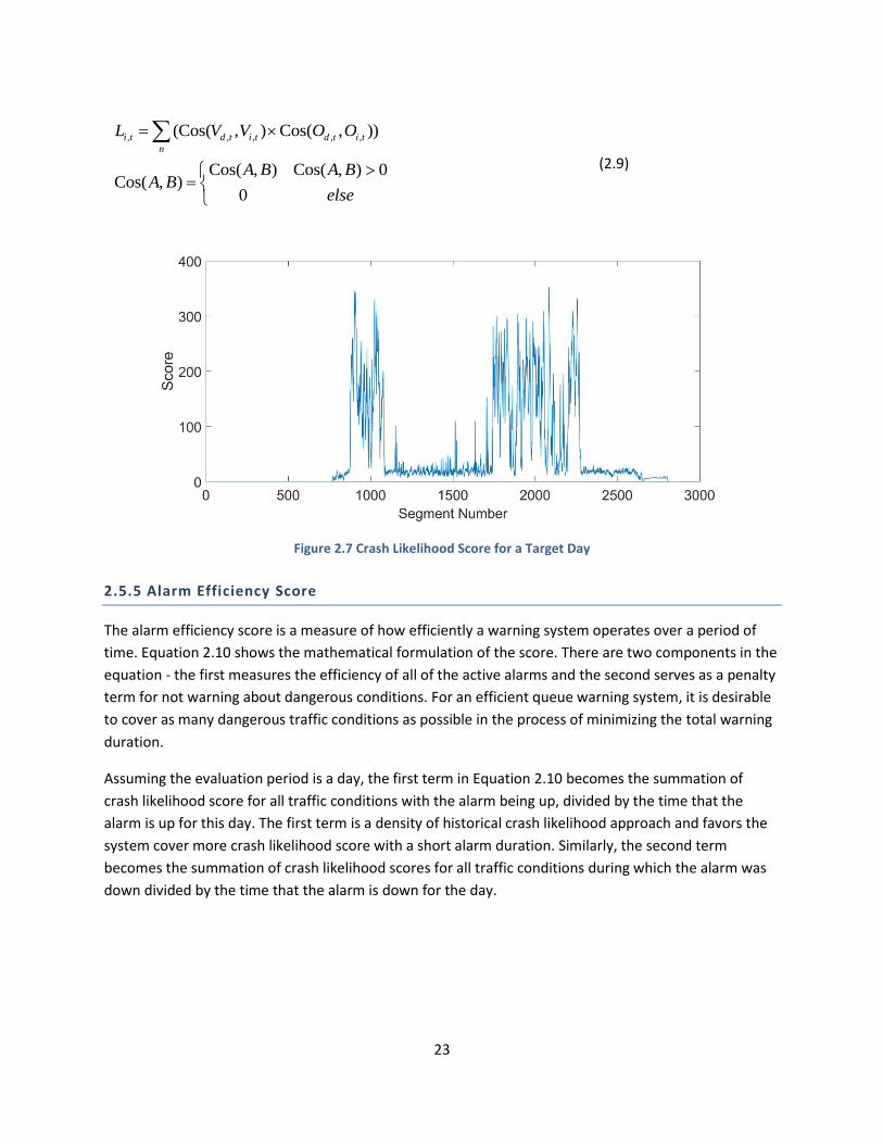
23
, , , , ,(Cos( , ) Cos( , ))
Cos( , ) Cos( , ) 0Cos( , )
0
i t d t i t d t i t
n
L V V O O
A B A BA B
else
(2.9)
Figure 2.7 Crash Likelihood Score for a Target Day
2.5.5 Alarm Efficiency Score
The alarm efficiency score is a measure of how efficiently a warning system operates over a period of
time. Equation 2.10 shows the mathematical formulation of the score. There are two components in the
equation - the first measures the efficiency of all of the active alarms and the second serves as a penalty
term for not warning about dangerous conditions. For an efficient queue warning system, it is desirable
to cover as many dangerous traffic conditions as possible in the process of minimizing the total warning
duration.
Assuming the evaluation period is a day, the first term in Equation 2.10 becomes the summation of
crash likelihood score for all traffic conditions with the alarm being up, divided by the time that the
alarm is up for this day. The first term is a density of historical crash likelihood approach and favors the
system cover more crash likelihood score with a short alarm duration. Similarly, the second term
becomes the summation of crash likelihood scores for all traffic conditions during which the alarm was
down divided by the time that the alarm is down for the day.
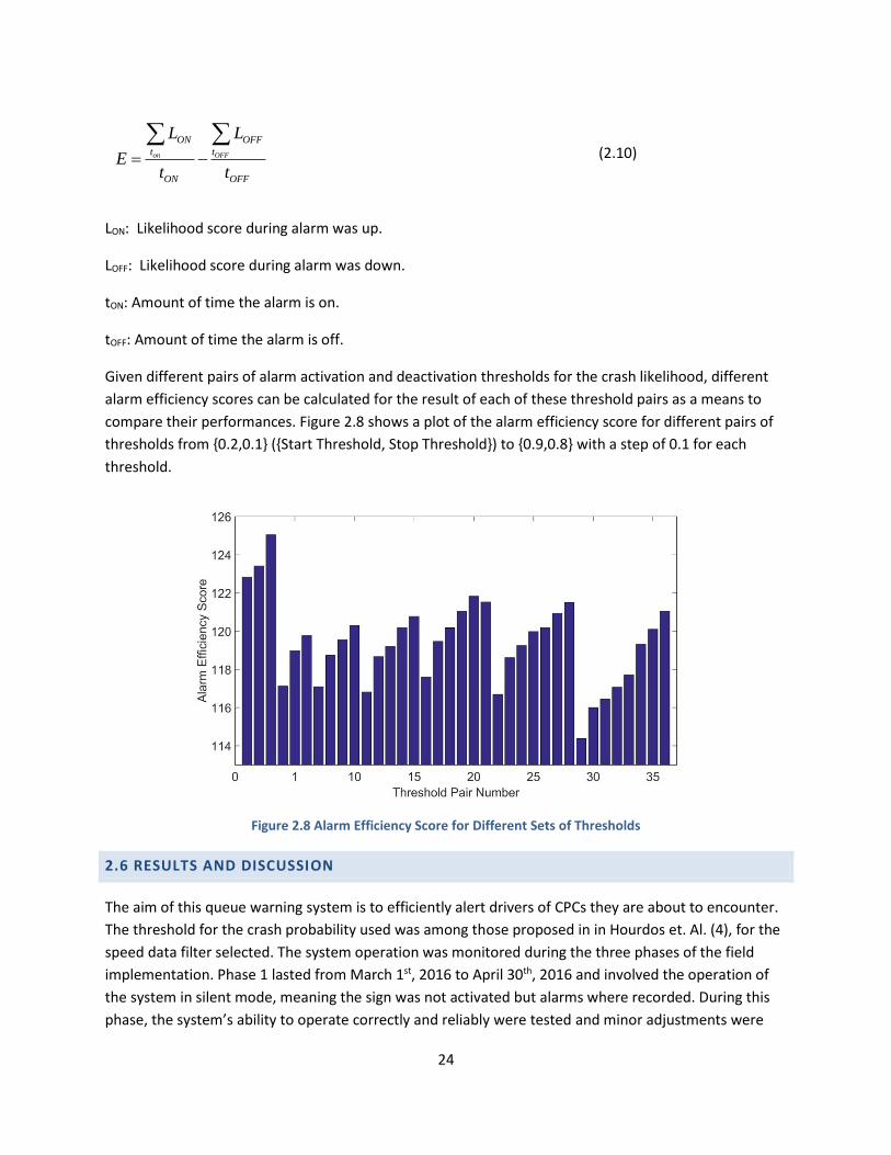
24
on OFF
ON OFF
t t
ON OFF
L L
Et t
(2.10)
LON: Likelihood score during alarm was up.
LOFF: Likelihood score during alarm was down.
tON: Amount of time the alarm is on.
tOFF: Amount of time the alarm is off.
Given different pairs of alarm activation and deactivation thresholds for the crash likelihood, different
alarm efficiency scores can be calculated for the result of each of these threshold pairs as a means to
compare their performances. Figure 2.8 shows a plot of the alarm efficiency score for different pairs of
thresholds from {0.2,0.1} ({Start Threshold, Stop Threshold}) to {0.9,0.8} with a step of 0.1 for each
threshold.
Figure 2.8 Alarm Efficiency Score for Different Sets of Thresholds
2.6 RESULTS AND DISCUSSION
The aim of this queue warning system is to efficiently alert drivers of CPCs they are about to encounter.
The threshold for the crash probability used was among those proposed in in Hourdos et. Al. (4), for the
speed data filter selected. The system operation was monitored during the three phases of the field
implementation. Phase 1 lasted from March 1st, 2016 to April 30th, 2016 and involved the operation of
the system in silent mode, meaning the sign was not activated but alarms where recorded. During this
phase, the system’s ability to operate correctly and reliably were tested and minor adjustments were
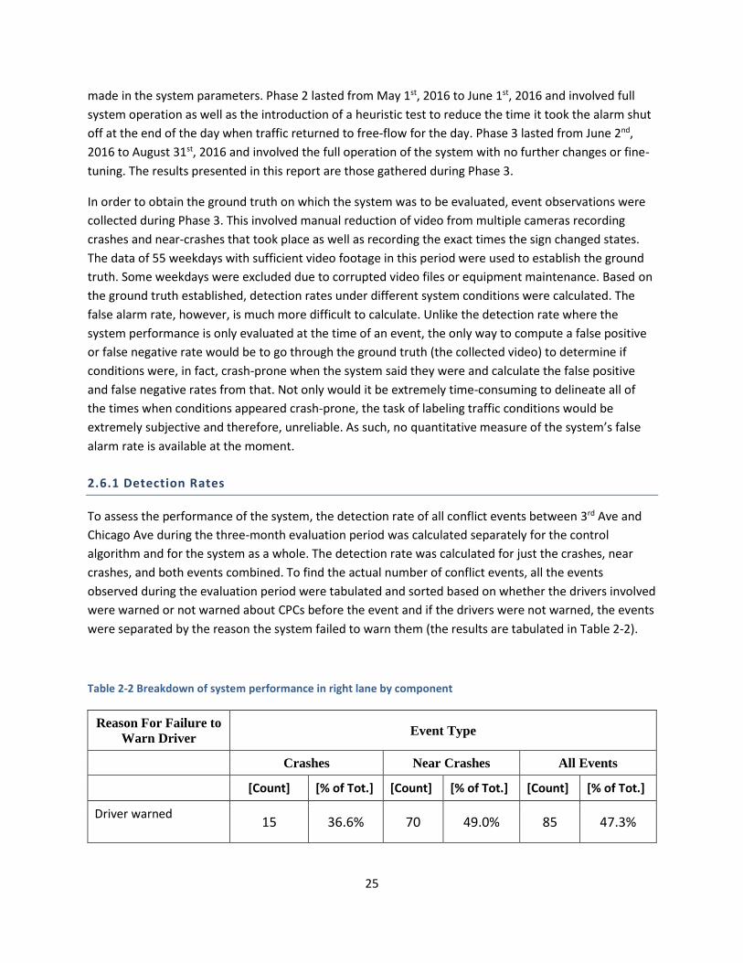
25
made in the system parameters. Phase 2 lasted from May 1st, 2016 to June 1st, 2016 and involved full
system operation as well as the introduction of a heuristic test to reduce the time it took the alarm shut
off at the end of the day when traffic returned to free-flow for the day. Phase 3 lasted from June 2nd,
2016 to August 31st, 2016 and involved the full operation of the system with no further changes or fine-
tuning. The results presented in this report are those gathered during Phase 3.
In order to obtain the ground truth on which the system was to be evaluated, event observations were
collected during Phase 3. This involved manual reduction of video from multiple cameras recording
crashes and near-crashes that took place as well as recording the exact times the sign changed states.
The data of 55 weekdays with sufficient video footage in this period were used to establish the ground
truth. Some weekdays were excluded due to corrupted video files or equipment maintenance. Based on
the ground truth established, detection rates under different system conditions were calculated. The
false alarm rate, however, is much more difficult to calculate. Unlike the detection rate where the
system performance is only evaluated at the time of an event, the only way to compute a false positive
or false negative rate would be to go through the ground truth (the collected video) to determine if
conditions were, in fact, crash-prone when the system said they were and calculate the false positive
and false negative rates from that. Not only would it be extremely time-consuming to delineate all of
the times when conditions appeared crash-prone, the task of labeling traffic conditions would be
extremely subjective and therefore, unreliable. As such, no quantitative measure of the system’s false
alarm rate is available at the moment.
2.6.1 Detection Rates
To assess the performance of the system, the detection rate of all conflict events between 3rd Ave and
Chicago Ave during the three-month evaluation period was calculated separately for the control
algorithm and for the system as a whole. The detection rate was calculated for just the crashes, near
crashes, and both events combined. To find the actual number of conflict events, all the events
observed during the evaluation period were tabulated and sorted based on whether the drivers involved
were warned or not warned about CPCs before the event and if the drivers were not warned, the events
were separated by the reason the system failed to warn them (the results are tabulated in Table 2-2).
Table 2-2 Breakdown of system performance in right lane by component
Reason For Failure to
Warn Driver Event Type
Crashes Near Crashes All Events
[Count] [% of Tot.] [Count] [% of Tot.] [Count] [% of Tot.]
Driver warned
15 36.6% 70 49.0% 85 47.3%
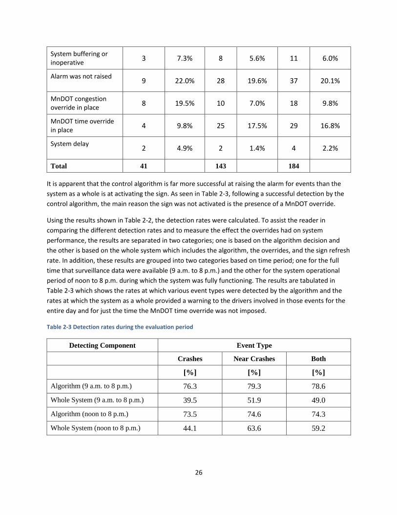
26
System buffering or inoperative
3 7.3% 8 5.6% 11 6.0%
Alarm was not raised
9 22.0% 28 19.6% 37 20.1%
MnDOT congestion override in place
8 19.5% 10 7.0% 18 9.8%
MnDOT time override in place
4 9.8% 25 17.5% 29 16.8%
System delay
2 4.9% 2 1.4% 4 2.2%
Total 41 143 184
It is apparent that the control algorithm is far more successful at raising the alarm for events than the
system as a whole is at activating the sign. As seen in Table 2-3, following a successful detection by the
control algorithm, the main reason the sign was not activated is the presence of a MnDOT override.
Using the results shown in Table 2-2, the detection rates were calculated. To assist the reader in
comparing the different detection rates and to measure the effect the overrides had on system
performance, the results are separated in two categories; one is based on the algorithm decision and
the other is based on the whole system which includes the algorithm, the overrides, and the sign refresh
rate. In addition, these results are grouped into two categories based on time period; one for the full
time that surveillance data were available (9 a.m. to 8 p.m.) and the other for the system operational
period of noon to 8 p.m. during which the system was fully functioning. The results are tabulated in
Table 2-3 which shows the rates at which various event types were detected by the algorithm and the
rates at which the system as a whole provided a warning to the drivers involved in those events for the
entire day and for just the time the MnDOT time override was not imposed.
Table 2-3 Detection rates during the evaluation period
Detecting Component Event Type
Crashes Near Crashes Both
[%] [%] [%]
Algorithm (9 a.m. to 8 p.m.) 76.3 79.3 78.6
Whole System (9 a.m. to 8 p.m.) 39.5 51.9 49.0
Algorithm (noon to 8 p.m.) 73.5 74.6 74.3
Whole System (noon to 8 p.m.) 44.1 63.6 59.2
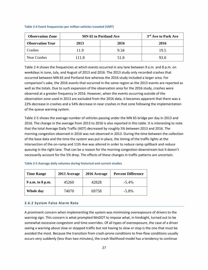
27
Table 2-4 Event frequencies per million vehicles traveled (VMT)
Observation Zone MN 65 to Portland Ave 3rd Ave to Park Ave
Observation Year 2013 2016 2016
Crashes 11.9 9.34 19.5
Near Crashes 111.8 51.8 93.0
Table 2-4 shows the frequencies at which events occurred in any lane between 9 a.m. and 8 p.m. on
weekdays in June, July, and August of 2013 and 2016. The 2013 study only recorded crashes that
occurred between MN 65 and Portland Ave whereas the 2016 study included a larger area. For
comparison’s sake, the 2016 events that occurred in the same region as the 2013 events are reported as
well as the totals. Due to such expansion of the observation area for the 2016 study, crashes were
observed at a greater frequency in 2016. However, when the events occurring outside of the
observation zone used in 2013 are excluded from the 2016 data, it becomes apparent that there was a
22% decrease in crashes and a 54% decrease in near crashes in that zone following the implementation
of the queue warning system.
Table 2-5 shows the average number of vehicles passing under the MN 65 bridge per day in 2013 and
2016. The change in the average from 2013 to 2016 is also reported in this table. It is interesting to note
that the total Average Daily Traffic (ADT) decreased by roughly 5% between 2013 and 2016. The
morning congestion observed in 2016 was not observed in 2013. During the time between the collection
of the base data and the time the system was put in place, the timing of the traffic lights at the
intersection of the on-ramp and 11th Ave was altered in order to reduce ramp spillback and reduce
queuing in the right lane. That can be a reason for the morning congestion downstream but it doesn’t
necessarily account for the 5% drop. The effects of these changes in traffic patterns are uncertain.
Table 2-5 Average daily volumes during historical and current studies
Time Range 2013 Average 2016 Average Percent Difference
9 a.m. to 8 p.m. 45260 42828 -5.4%
Whole day 74070 69758 -5.8%
2.6.2 System False Alarm Rate
A prominent concern when implementing the system was minimizing overexposure of drivers to the
warning sign. This concern is what prompted MnDOT to impose what, in hindsight, turned out to be
somewhat excessive congestion and time overrides. Of all types of overexposure, the case of a driver
seeing a warning about slow or stopped traffic but not having to slow or stop is the one that must be
avoided the most. Because the transition from crash-prone conditions to free-flow conditions usually
occurs very suddenly (less than two minutes), the crash likelihood model has a tendency to continue
28
outputting crash probabilities indicative of crash-prone conditions for up to 15 minutes after
uncongested flow conditions have been restored. In order to reduce the false alarm rate coming from
this delay, an override was built into the control algorithm to deactivate the alarm, regardless of the
model result at the time, when both MVDs observe 10 consecutive vehicles with speeds greater than 30
mph.
2.6.3 System Limitations
Due to the fact that the system is still in the prototype phase, several aspects of it are less than ideal and
result in uncertainties of varying degrees. The limitations and uncertainties include the non-ideal
configurations of the MVDs and warning sign, the limitations of the hardware, the fact that some of the
equipment was shared with MnDOT, and the fact that the model result is currently computed for only
the right lane. In the interest of cost and time, the MVDs were installed on a high-rise near the road
rather than on a gantry or bridge directly over the road. The warning messages were displayed on the
relatively small MnDOT changeable message board rather than a purpose-made display with potentially
different characteristics (location, size, color, etc.). The limitations of the hardware also presented a
source of uncertainty in that the speed data from the MnDOT single loop detector was only a 30-second
average and was not completely accurate. Issues with power outages and lack of sufficient data storage
at the rooftop station resulted in missing video data. Because control of the sign and the camera
monitoring was shared with MnDOT, the sign was occasionally used to display incident management
messages from MnDOT rather than the queue warning messages. Because the capability of the system
to function as intended and the effect that it would have on drivers were unknown at the time of
installation, it was only applied to one of the three lanes. As a result, it is unclear what effect this partial
deployment had on driver's actions.
2.7 CONCLUSIONS
Impressions from the 55 weekdays of evaluation in the summer of 2016 suggest that the queue warning
system prototype discussed in this report represents a successful crash prevention solution. The effect
of the system on conflict events is difficult to determine from the data available but the system
performs well given the constraints under which it is operating. The system raised the alarm for 79% of
all conflict events that occurred during the evaluation period but was only able to warn drivers for 49%
of all conflict events predominantly due to the overrides that were put in place to prevent the possibility
of the system displaying the warning for excessive amounts of time. Why these crashes happened even
with the drivers exposed to the warning is unknown. One can speculate that the message is not clear or
strong enough. A lot of the vehicles involved are only exposed to the warning once on the Park Ave
gantry since the warning sign further upstream is not visible from the entrance from 35W SB. The
project was supposed to test different messages but due to time delays at both ends this did not
happen. Regardless, if more messages were tested in the same period it would have been difficult to
gauge the driver response since events are still infrequent and random.

29
Now that proof of concept has been confirmed, the next step will be to expand and optimize the
infrastructure used by the system. Several changes to the system on the policy and infrastructure levels
have been identified that will likely result in greater detection and warning rates and thereby decreased
conflict event rates. Given greater design control, many of the system limitations could be mitigated if
not eliminated altogether. This will include installing MVDs or other sensors on gantries or bridges
directly above the freeway in so they are afforded a stable head-on view of traffic and placing the
warning sign in a location selected by choice rather than necessity. The warning sign shape, size,
location, and message may also need to be optimized to increase driver attention. The most important
improvement will be expanding the system to all three lanes of traffic and following that change with a
long-term study of the effects of the system on conflict event frequencies.
30
DEVELOPMENT AND FIELD DEPLOYMENT OF A
QUEUE WARNING SYSTEM ON I-35W SB BASED ON FREEWAY
QUEUE LENGTH ESTIMATION
3.1 PROJECT MOTIVATION
Past research studies have shown that freeway rear-end collisions tend to occur in extended stop-and-
go traffic or at end-of-queue locations (29). By identifying these kinds of traffic conditions and providing
warning messages to drivers before they encounter those conditions, drivers are more alert of and
prepared for crash prone conditions (CPCs) thereby reducing the likelihood of traffic accidents. This, in
turn, improves mobility because severe traffic congestion caused by traffic accidents can be avoided or
alleviated. This project holds the potential to improve both traffic safety and mobility.
3.2 PROJECT OBJECTIVES
The project objectives are:
1. Capitalize on past research and existing and new traffic detection capabilities on I-94 and new
instrumentation on I-35W to develop a CPC detection system capable of generating alarms
when the danger for rear-end collisions is high.
2. The project will evaluate potential driver warning messages that can be displayed by the
existing intelligent lane crash signal (ILCS) and select the ones that are most effective in raising
drivers’ attention levels.
3. Finally, the project will develop a working prototype for the Rear-End Collision Prevention
Driver Warning system and assist Minnesota Department of Transportation (MnDOT) in field
implementation and testing.
3.3 LITERATURE REVIEW
3.3.1 Literature Review on Freeway Queue Length Estimation
Real-time prediction of the length of queues on freeways is of great help for the development of
advanced freeway traffic management systems. Since the 1960s (42, 66, 76, 45), the importance of
managing vehicle queue length to reduce vehicle delay and prevent spillover, especially at signalized
intersections, has been recognized and studied (39, 40, 31, 62, 63, 35, 65).
3.3.1.1 Basic Methodology on Queue Length Estimation
Essentially, two basic approaches have been developed to estimate queue length, namely the
cumulative traffic input-output methods and the shockwave methods.
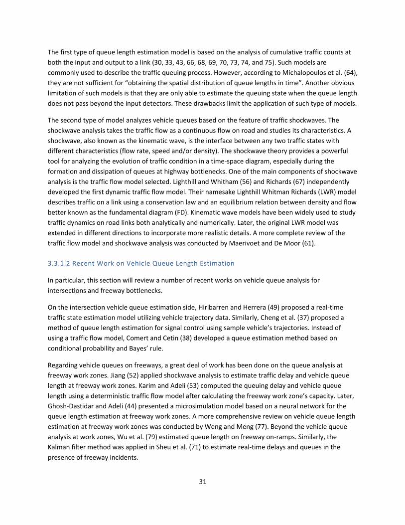
31
The first type of queue length estimation model is based on the analysis of cumulative traffic counts at
both the input and output to a link (30, 33, 43, 66, 68, 69, 70, 73, 74, and 75). Such models are
commonly used to describe the traffic queuing process. However, according to Michalopoulos et al. (64),
they are not sufficient for “obtaining the spatial distribution of queue lengths in time”. Another obvious
limitation of such models is that they are only able to estimate the queuing state when the queue length
does not pass beyond the input detectors. These drawbacks limit the application of such type of models.
The second type of model analyzes vehicle queues based on the feature of traffic shockwaves. The
shockwave analysis takes the traffic flow as a continuous flow on road and studies its characteristics. A
shockwave, also known as the kinematic wave, is the interface between any two traffic states with
different characteristics (flow rate, speed and/or density). The shockwave theory provides a powerful
tool for analyzing the evolution of traffic condition in a time-space diagram, especially during the
formation and dissipation of queues at highway bottlenecks. One of the main components of shockwave
analysis is the traffic flow model selected. Lighthill and Whitham (56) and Richards (67) independently
developed the first dynamic traffic flow model. Their namesake Lighthill Whitman Richards (LWR) model
describes traffic on a link using a conservation law and an equilibrium relation between density and flow
better known as the fundamental diagram (FD). Kinematic wave models have been widely used to study
traffic dynamics on road links both analytically and numerically. Later, the original LWR model was
extended in different directions to incorporate more realistic details. A more complete review of the
traffic flow model and shockwave analysis was conducted by Maerivoet and De Moor (61).
3.3.1.2 Recent Work on Vehicle Queue Length Estimation
In particular, this section will review a number of recent works on vehicle queue analysis for
intersections and freeway bottlenecks.
On the intersection vehicle queue estimation side, Hiribarren and Herrera (49) proposed a real-time
traffic state estimation model utilizing vehicle trajectory data. Similarly, Cheng et al. (37) proposed a
method of queue length estimation for signal control using sample vehicle’s trajectories. Instead of
using a traffic flow model, Comert and Cetin (38) developed a queue estimation method based on
conditional probability and Bayes’ rule.
Regarding vehicle queues on freeways, a great deal of work has been done on the queue analysis at
freeway work zones. Jiang (52) applied shockwave analysis to estimate traffic delay and vehicle queue
length at freeway work zones. Karim and Adeli (53) computed the queuing delay and vehicle queue
length using a deterministic traffic flow model after calculating the freeway work zone’s capacity. Later,
Ghosh-Dastidar and Adeli (44) presented a microsimulation model based on a neural network for the
queue length estimation at freeway work zones. A more comprehensive review on vehicle queue length
estimation at freeway work zones was conducted by Weng and Meng (77). Beyond the vehicle queue
analysis at work zones, Wu et al. (79) estimated queue length on freeway on-ramps. Similarly, the
Kalman filter method was applied in Sheu et al. (71) to estimate real-time delays and queues in the
presence of freeway incidents.
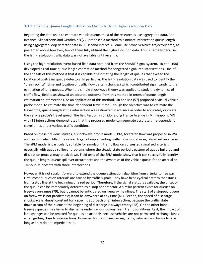
32
3.3.1.3 Vehicle Queue Length Estimation Methods Using High-Resolution Data
Regarding the data used to estimate vehicle queue, most of the researches use aggregated data. For
instance, Skabardonis and Geroliminis (72) proposed a method to estimate intersection queue length
using aggregated loop detector data in 30-second intervals. Some use probe vehicles’ trajectory data, as
presented above however, few of them fully utilized the high-resolution data. This is partially because
the high-resolution traffic data was not available until recently.
Using the high-resolution event-based field data obtained from the SMART-Signal system, Liu et al. (58)
developed a real-time queue length estimation method for congested signalized intersections. One of
the appeals of this method is that it is capable of estimating the length of queues that exceed the
location of upstream queue detectors. In particular, the high-resolution data was used to identify the
“break points” (time and location of traffic flow pattern changes) which contributed significantly to the
estimation of long queues. When the simple shockwave theory was applied to study the dynamics of
traffic flow, field tests showed an accurate outcome from this method in terms of queue length
estimation at intersections. As an application of this method, Liu and Ma (57) proposed a virtual vehicle
probe model to estimate the time-dependent travel time. Though the objective was to estimate the
travel time, queue length at the intersection was estimated in advance in order to accurately calculate
the vehicle probe’s travel speed. The field test on a corridor along France Avenue in Minneapolis, MN
with 11 intersections demonstrated that the proposed model can generate accurate time-dependent
travel times under various traffic conditions.
Based on these previous studies, a shockwave profile model (SPM) for traffic flow was proposed in Wu
and Liu (80) which filled the research gap of implementing traffic flow model in signalized urban arterial.
The SPM model is particularly suitable for simulating traffic flow on congested signalized arterials
especially with queue spillover problems where the steady-state periodic pattern of queue build-up and
dissipation process may break down. Field tests of the SPM model show that it can successfully identify
the queue length, queue spillover occurrences and the dynamics of the vehicle queue for an arterial on
TH-55 in Minnesota with three intersections.
However, it is not straightforward to extend the queue estimation algorithm from arterial to freeway. First, most queues on arterials are caused by traffic signals. They have fixed cyclical pattern that starts from a stop line at the beginning of a red period. Therefore, if the signal status is available, the onset of the queue can be immediately detected by a stop bar detector. A similar pattern exists for queues on freeway on-ramps (79), but it cannot be anticipated on freeway mainlines. The start of a stopped queue on freeways is not predictable; it can be anywhere at any time (41). Second, the speed of discharge shockwave is almost constant for a specific approach of an intersection, because the traffic state downstream of the queue at the beginning of discharge is always empty (58). On the other hand, freeway queues may begin to discharge under various downstream traffic conditions. Last, the impact of lane changes can be omitted for queues on arterials because vehicles are not permitted to change lanes when getting close to intersections. However, for most freeway segments, vehicles can change lane as long as they do not impede others.
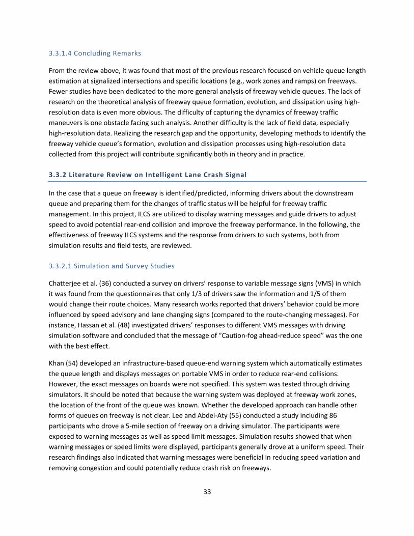
33
3.3.1.4 Concluding Remarks
From the review above, it was found that most of the previous research focused on vehicle queue length
estimation at signalized intersections and specific locations (e.g., work zones and ramps) on freeways.
Fewer studies have been dedicated to the more general analysis of freeway vehicle queues. The lack of
research on the theoretical analysis of freeway queue formation, evolution, and dissipation using high-
resolution data is even more obvious. The difficulty of capturing the dynamics of freeway traffic
maneuvers is one obstacle facing such analysis. Another difficulty is the lack of field data, especially
high-resolution data. Realizing the research gap and the opportunity, developing methods to identify the
freeway vehicle queue’s formation, evolution and dissipation processes using high-resolution data
collected from this project will contribute significantly both in theory and in practice.
3.3.2 Literature Review on Intelligent Lane Crash Signal
In the case that a queue on freeway is identified/predicted, informing drivers about the downstream
queue and preparing them for the changes of traffic status will be helpful for freeway traffic
management. In this project, ILCS are utilized to display warning messages and guide drivers to adjust
speed to avoid potential rear-end collision and improve the freeway performance. In the following, the
effectiveness of freeway ILCS systems and the response from drivers to such systems, both from
simulation results and field tests, are reviewed.
3.3.2.1 Simulation and Survey Studies
Chatterjee et al. (36) conducted a survey on drivers’ response to variable message signs (VMS) in which
it was found from the questionnaires that only 1/3 of drivers saw the information and 1/5 of them
would change their route choices. Many research works reported that drivers’ behavior could be more
influenced by speed advisory and lane changing signs (compared to the route-changing messages). For
instance, Hassan et al. (48) investigated drivers’ responses to different VMS messages with driving
simulation software and concluded that the message of “Caution-fog ahead-reduce speed” was the one
with the best effect.
Khan (54) developed an infrastructure-based queue-end warning system which automatically estimates
the queue length and displays messages on portable VMS in order to reduce rear-end collisions.
However, the exact messages on boards were not specified. This system was tested through driving
simulators. It should be noted that because the warning system was deployed at freeway work zones,
the location of the front of the queue was known. Whether the developed approach can handle other
forms of queues on freeway is not clear. Lee and Abdel-Aty (55) conducted a study including 86
participants who drove a 5-mile section of freeway on a driving simulator. The participants were
exposed to warning messages as well as speed limit messages. Simulation results showed that when
warning messages or speed limits were displayed, participants generally drove at a uniform speed. Their
research findings also indicated that warning messages were beneficial in reducing speed variation and
removing congestion and could potentially reduce crash risk on freeways.
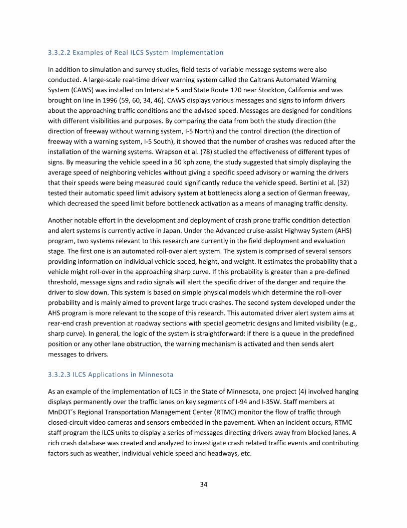
34
3.3.2.2 Examples of Real ILCS System Implementation
In addition to simulation and survey studies, field tests of variable message systems were also
conducted. A large-scale real-time driver warning system called the Caltrans Automated Warning
System (CAWS) was installed on Interstate 5 and State Route 120 near Stockton, California and was
brought on line in 1996 (59, 60, 34, 46). CAWS displays various messages and signs to inform drivers
about the approaching traffic conditions and the advised speed. Messages are designed for conditions
with different visibilities and purposes. By comparing the data from both the study direction (the
direction of freeway without warning system, I-5 North) and the control direction (the direction of
freeway with a warning system, I-5 South), it showed that the number of crashes was reduced after the
installation of the warning systems. Wrapson et al. (78) studied the effectiveness of different types of
signs. By measuring the vehicle speed in a 50 kph zone, the study suggested that simply displaying the
average speed of neighboring vehicles without giving a specific speed advisory or warning the drivers
that their speeds were being measured could significantly reduce the vehicle speed. Bertini et al. (32)
tested their automatic speed limit advisory system at bottlenecks along a section of German freeway,
which decreased the speed limit before bottleneck activation as a means of managing traffic density.
Another notable effort in the development and deployment of crash prone traffic condition detection
and alert systems is currently active in Japan. Under the Advanced cruise-assist Highway System (AHS)
program, two systems relevant to this research are currently in the field deployment and evaluation
stage. The first one is an automated roll-over alert system. The system is comprised of several sensors
providing information on individual vehicle speed, height, and weight. It estimates the probability that a
vehicle might roll-over in the approaching sharp curve. If this probability is greater than a pre-defined
threshold, message signs and radio signals will alert the specific driver of the danger and require the
driver to slow down. This system is based on simple physical models which determine the roll-over
probability and is mainly aimed to prevent large truck crashes. The second system developed under the
AHS program is more relevant to the scope of this research. This automated driver alert system aims at
rear-end crash prevention at roadway sections with special geometric designs and limited visibility (e.g.,
sharp curve). In general, the logic of the system is straightforward: if there is a queue in the predefined
position or any other lane obstruction, the warning mechanism is activated and then sends alert
messages to drivers.
3.3.2.3 ILCS Applications in Minnesota
As an example of the implementation of ILCS in the State of Minnesota, one project (4) involved hanging
displays permanently over the traffic lanes on key segments of I-94 and I-35W. Staff members at
MnDOT’s Regional Transportation Management Center (RTMC) monitor the flow of traffic through
closed-circuit video cameras and sensors embedded in the pavement. When an incident occurs, RTMC
staff program the ILCS units to display a series of messages directing drivers away from blocked lanes. A
rich crash database was created and analyzed to investigate crash related traffic events and contributing
factors such as weather, individual vehicle speed and headways, etc.
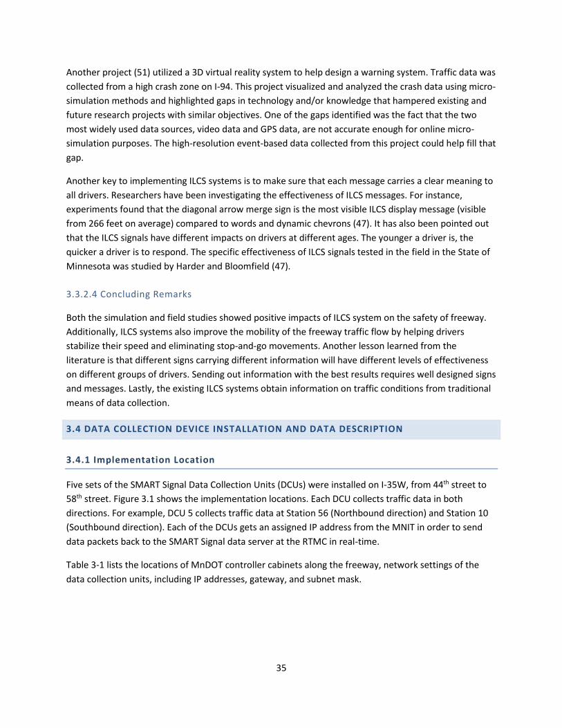
35
Another project (51) utilized a 3D virtual reality system to help design a warning system. Traffic data was
collected from a high crash zone on I-94. This project visualized and analyzed the crash data using micro-
simulation methods and highlighted gaps in technology and/or knowledge that hampered existing and
future research projects with similar objectives. One of the gaps identified was the fact that the two
most widely used data sources, video data and GPS data, are not accurate enough for online micro-
simulation purposes. The high-resolution event-based data collected from this project could help fill that
gap.
Another key to implementing ILCS systems is to make sure that each message carries a clear meaning to
all drivers. Researchers have been investigating the effectiveness of ILCS messages. For instance,
experiments found that the diagonal arrow merge sign is the most visible ILCS display message (visible
from 266 feet on average) compared to words and dynamic chevrons (47). It has also been pointed out
that the ILCS signals have different impacts on drivers at different ages. The younger a driver is, the
quicker a driver is to respond. The specific effectiveness of ILCS signals tested in the field in the State of
Minnesota was studied by Harder and Bloomfield (47).
3.3.2.4 Concluding Remarks
Both the simulation and field studies showed positive impacts of ILCS system on the safety of freeway.
Additionally, ILCS systems also improve the mobility of the freeway traffic flow by helping drivers
stabilize their speed and eliminating stop-and-go movements. Another lesson learned from the
literature is that different signs carrying different information will have different levels of effectiveness
on different groups of drivers. Sending out information with the best results requires well designed signs
and messages. Lastly, the existing ILCS systems obtain information on traffic conditions from traditional
means of data collection.
3.4 DATA COLLECTION DEVICE INSTALLATION AND DATA DESCRIPTION
3.4.1 Implementation Location
Five sets of the SMART Signal Data Collection Units (DCUs) were installed on I-35W, from 44th street to
58th street. Figure 3.1 shows the implementation locations. Each DCU collects traffic data in both
directions. For example, DCU 5 collects traffic data at Station 56 (Northbound direction) and Station 10
(Southbound direction). Each of the DCUs gets an assigned IP address from the MNIT in order to send
data packets back to the SMART Signal data server at the RTMC in real-time.
Table 3-1 lists the locations of MnDOT controller cabinets along the freeway, network settings of the
data collection units, including IP addresses, gateway, and subnet mask.
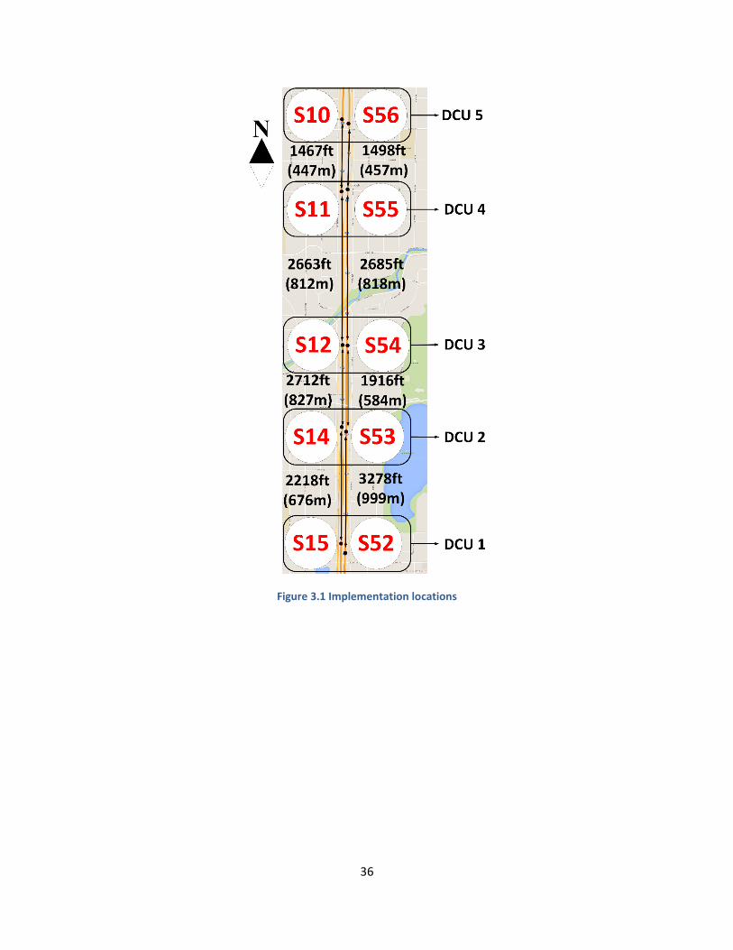
36
Figure 3.1 Implementation locations
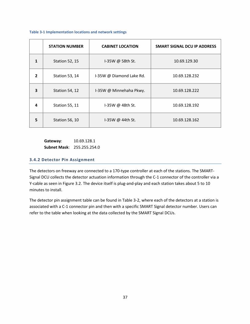
37
Table 3-1 Implementation locations and network settings
STATION NUMBER CABINET LOCATION SMART SIGNAL DCU IP ADDRESS
1 Station 52, 15 I-35W @ 58th St. 10.69.129.30
2 Station 53, 14 I-35W @ Diamond Lake Rd. 10.69.128.232
3 Station 54, 12 I-35W @ Minnehaha Pkwy. 10.69.128.222
4 Station 55, 11 I-35W @ 48th St. 10.69.128.192
5 Station 56, 10 I-35W @ 44th St. 10.69.128.162
Gateway: 10.69.128.1
Subnet Mask: 255.255.254.0
3.4.2 Detector Pin Assignment
The detectors on freeway are connected to a 170-type controller at each of the stations. The SMART-
Signal DCU collects the detector actuation information through the C-1 connector of the controller via a
Y-cable as seen in Figure 3.2. The device itself is plug-and-play and each station takes about 5 to 10
minutes to install.
The detector pin assignment table can be found in Table 3-2, where each of the detectors at a station is
associated with a C-1 connector pin and then with a specific SMART Signal detector number. Users can
refer to the table when looking at the data collected by the SMART Signal DCUs.
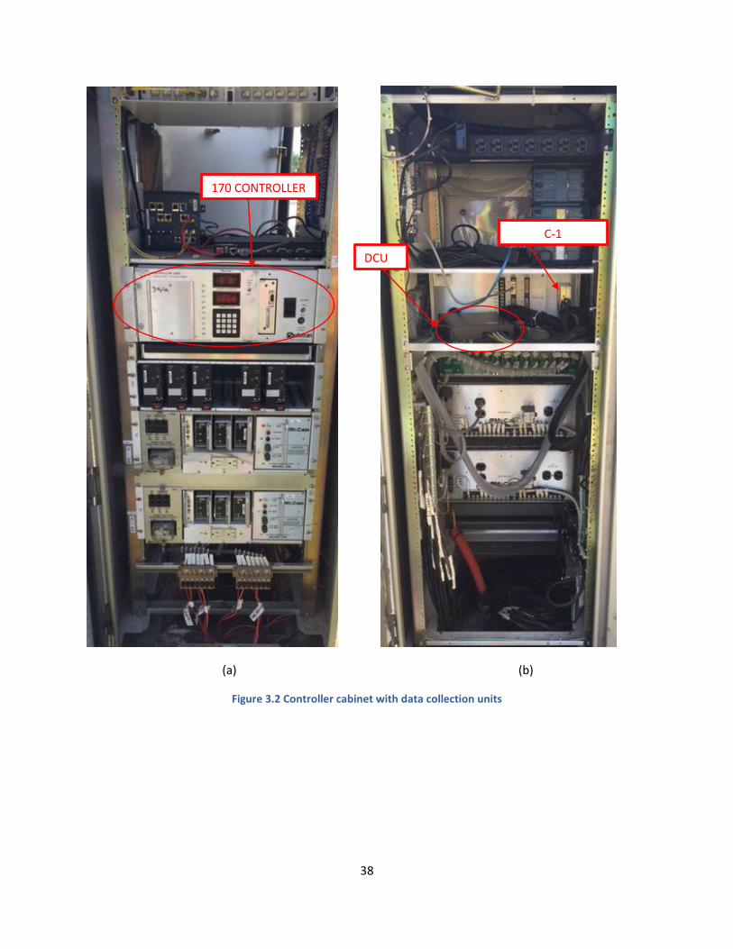
38
(a) (b)
Figure 3.2 Controller cabinet with data collection units
DCU
170 CONTROLLER
C-1
CONNECTOR
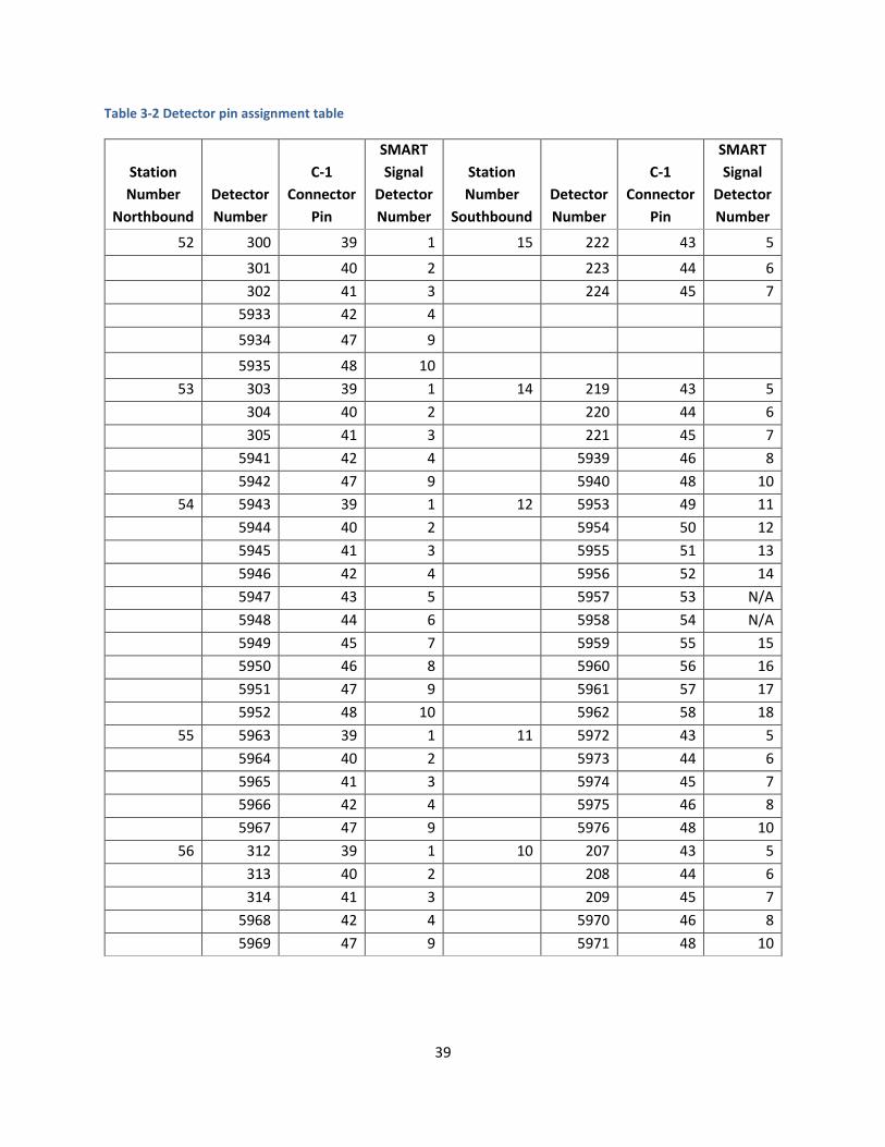
39
Table 3-2 Detector pin assignment table
Station
Number
Northbound
Detector
Number
C-1
Connector
Pin
SMART
Signal
Detector
Number
Station
Number
Southbound
Detector
Number
C-1
Connector
Pin
SMART
Signal
Detector
Number
52 300 39 1 15 222 43 5
301 40 2 223 44 6
302 41 3 224 45 7
5933 42 4
5934 47 9
5935 48 10
53 303 39 1 14 219 43 5
304 40 2 220 44 6
305 41 3 221 45 7
5941 42 4 5939 46 8
5942 47 9 5940 48 10
54 5943 39 1 12 5953 49 11
5944 40 2 5954 50 12
5945 41 3 5955 51 13
5946 42 4 5956 52 14
5947 43 5 5957 53 N/A
5948 44 6 5958 54 N/A
5949 45 7 5959 55 15
5950 46 8 5960 56 16
5951 47 9 5961 57 17
5952 48 10 5962 58 18
55 5963 39 1 11 5972 43 5
5964 40 2 5973 44 6
5965 41 3 5974 45 7
5966 42 4 5975 46 8
5967 47 9 5976 48 10
56 312 39 1 10 207 43 5
313 40 2 208 44 6
314 41 3 209 45 7
5968 42 4 5970 46 8
5969 47 9 5971 48 10
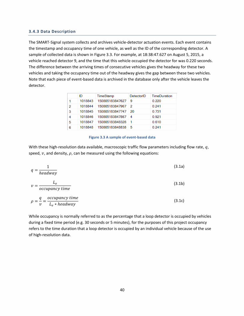
40
3.4.3 Data Description
The SMART-Signal system collects and archives vehicle-detector actuation events. Each event contains
the timestamp and occupancy time of one vehicle, as well as the ID of the corresponding detector. A
sample of collected data is shown in Figure 3.3. For example, at 18:38:47.627 on August 5, 2015, a
vehicle reached detector 9, and the time that this vehicle occupied the detector for was 0.220 seconds.
The difference between the arriving times of consecutive vehicles gives the headway for these two
vehicles and taking the occupancy time out of the headway gives the gap between these two vehicles.
Note that each piece of event-based data is archived in the database only after the vehicle leaves the
detector.
Figure 3.3 A sample of event-based data
With these high-resolution data available, macroscopic traffic flow parameters including flow rate, 𝑞,
speed, 𝑣, and density, 𝜌, can be measured using the following equations:
𝑞 =1
ℎ𝑒𝑎𝑑𝑤𝑎𝑦
𝑣 =𝐿𝑒
𝑜𝑐𝑐𝑢𝑝𝑎𝑛𝑐𝑦 𝑡𝑖𝑚𝑒
𝜌 =𝑞
𝑣=
𝑜𝑐𝑐𝑢𝑝𝑎𝑛𝑐𝑦 𝑡𝑖𝑚𝑒
𝐿𝑒 ∗ ℎ𝑒𝑎𝑑𝑤𝑎𝑦
(3.1a)
(3.1b)
(3.1c)
While occupancy is normally referred to as the percentage that a loop detector is occupied by vehicles
during a fixed time period (e.g. 30 seconds or 5 minutes), for the purposes of this project occupancy
refers to the time duration that a loop detector is occupied by an individual vehicle because of the use
of high-resolution data.

41
3.5 ALGORITHM DEVELOPMENT (I-35W TEST SITE)
3.5.1 Online Queue Length Estimation Algorithm
Before going into detail, it is necessary to define the applicable scope of the online queue length
estimation algorithm developed for this project. The onset of a stopped queue on freeway can occur
anywhere and at any time. Due to the limited number and fixed locations of loop detectors, the
occurrence time and position of the very first queued vehicle can rarely be identified. Based on the real-
time data collected from detectors, the algorithm can “see” the queue only when it travels to the
position of a detector. Although traffic states from detectors upstream and downstream of the queue
give some information on the queue, it is risky to predict the occurrence of a queue before it reaches a
detector because such prediction easily generates false alerts. Therefore, instead of capturing the exact
occurrence time and location of every stopped queue, the algorithm works to monitor the queue once it
is seen by detectors. For those queues starting from in-between positions and propagate to detectors,
lags in response arise but the algorithm provides a more robust solution than capturing the exact
occurrence time and location of every stopped queue. For those not propagating to detectors, the
algorithm omits them because of their limited influence in space and time.
The algorithm runs locally in any freeway segment between two detectors, estimating the length and
duration of a queue once it the queue is detected by the downstream detector. When the queue grows
past the upstream detector, the algorithm stops estimating it; further estimation of the queue would be
provided by the same algorithm running in the next upstream segment. Moreover, considering the
difference of traffic states across lanes (e.g., lanes to different directions of a divergent junction), one
algorithm runs for each lane. The algorithm also has limited capability predict the time when a queue
will be formed or cleared at any given position in a segment nor can it calculate the length of the queue
in the segment.
3.5.1.1 Identification of the Occurrence and Termination of Queues
The first step of the algorithm is to identify the occurrence and termination of a queue at detector
locations. Generally, the occurrence of queues can be identified by checking the values of occupancy
time. For example, if a vehicle has occupied the detector for ten seconds, it is safe to claim that this
vehicle is stopped in a queue. However, relying solely on occupancy time may miss detection of some
queues. The reason for this is that drivers may maintain following distances than detector length when
stopping thereby occasionally leaving the detection area blank. In this case, vehicles are queued but no
large occupancy time can be seen from the data. One example is shown in Figure 3.4. Occupancy time
and headway for each vehicle are plotted. Most of the long occupancy times and long headways appear
in pairs as denoted by the black circles, except for one event that is highlighted by the green circle. Note
that this long headway together with very short occupancy time cannot be caused by a lack of traffic
demand since it is during peak hours. Rather, this single long headway is caused by a vehicle stopped in
the queue right behind the detector.
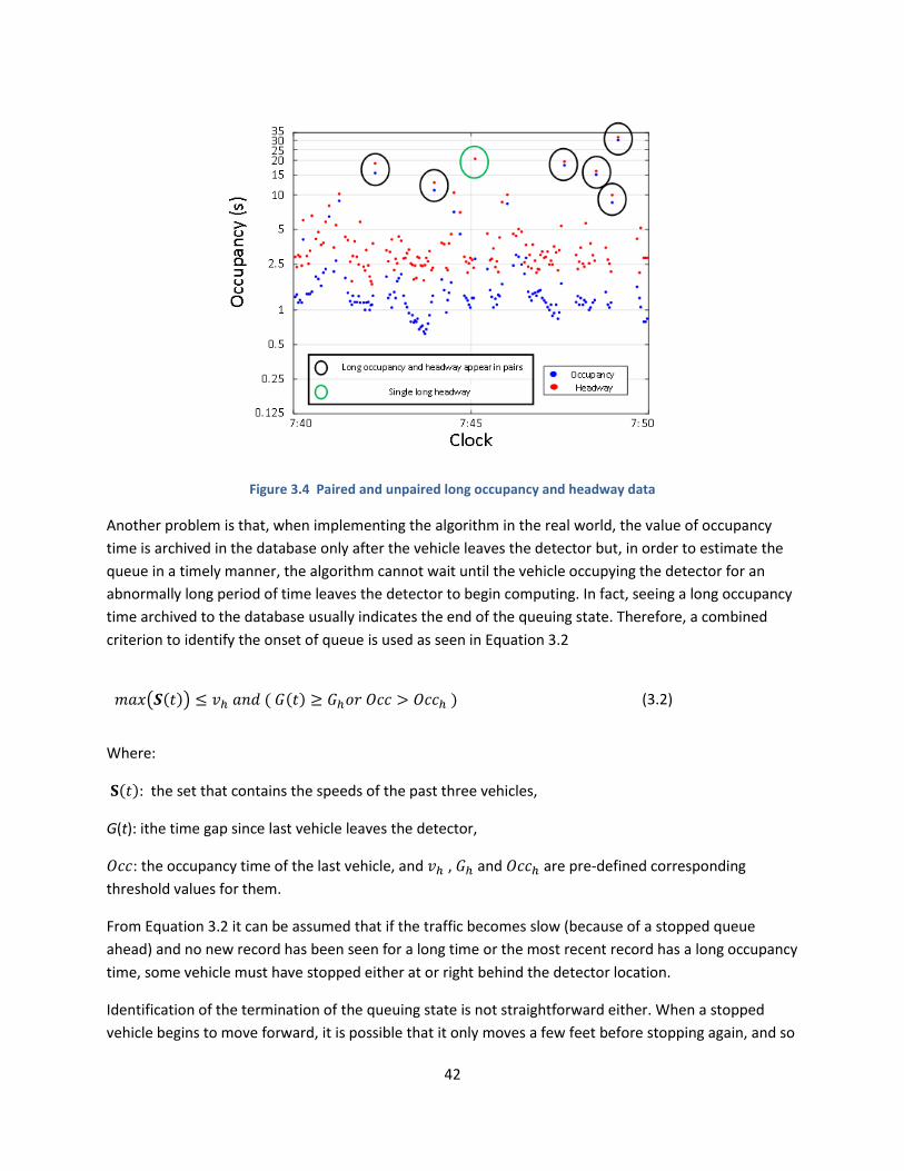
42
Figure 3.4 Paired and unpaired long occupancy and headway data
Another problem is that, when implementing the algorithm in the real world, the value of occupancy
time is archived in the database only after the vehicle leaves the detector but, in order to estimate the
queue in a timely manner, the algorithm cannot wait until the vehicle occupying the detector for an
abnormally long period of time leaves the detector to begin computing. In fact, seeing a long occupancy
time archived to the database usually indicates the end of the queuing state. Therefore, a combined
criterion to identify the onset of queue is used as seen in Equation 3.2
𝑚𝑎𝑥(𝑺(𝑡)) ≤ 𝑣ℎ 𝑎𝑛𝑑 ( 𝐺(𝑡) ≥ 𝐺ℎ𝑜𝑟 𝑂𝑐𝑐 > 𝑂𝑐𝑐ℎ ) (3.2)
Where:
𝐒(𝑡): the set that contains the speeds of the past three vehicles,
G(t): ithe time gap since last vehicle leaves the detector,
𝑂𝑐𝑐: the occupancy time of the last vehicle, and 𝑣ℎ , 𝐺ℎ and 𝑂𝑐𝑐ℎ are pre-defined corresponding
threshold values for them.
From Equation 3.2 it can be assumed that if the traffic becomes slow (because of a stopped queue
ahead) and no new record has been seen for a long time or the most recent record has a long occupancy
time, some vehicle must have stopped either at or right behind the detector location.
Identification of the termination of the queuing state is not straightforward either. When a stopped
vehicle begins to move forward, it is possible that it only moves a few feet before stopping again, and so

43
do the following vehicles. This happens often in freeway stop-and-go scenarios when the initial queue is
compressing. In this case, the move of the originally stopped vehicle does not mean the termination of
the queuing state. The termination of queuing state is, instead, confirmed by satisfying the following
equation
min (𝐒(𝑡)) ≥ 𝑣𝑙 (3.3)
Where:
𝐒(𝑡): the set that contains the speeds of the past three vehicles,
𝑣𝑙: another threshold value of speed.
3.5.1.2 Estimation of Queuing/Discharge Shockwave Speed
After identifying the onset and termination of queuing state, the algorithm will begin to estimate the
queue by calculating the positions of its head and tail. The theoretical basis of the algorithm is
shockwave theory. Shockwave takes place where two traffic states (e.g., free flow traffic state and jam
traffic state) meet. The speed of the shockwave w can be calculated by the following equation.
𝑤 =𝑞1 − 𝑞2
𝜌1 − 𝜌2 (3.4)
Where:
𝑞1,𝜌1:flow rate and density for upstream traffic
𝑞2 , 𝜌2: flow rate and density for downstream traffic, respectively.
Typically, there are two kinds of shockwaves in the queuing process on freeway: the queuing shockwave
that is described by the position of the last queued vehicle, i.e. queue tail, and the discharge shockwave
that is described by the position of the first vehicle waiting to be discharged, i.e. queue head. The traffic
states near the two shockwaves are shown in the time-space diagram in Figure 3.5. From left to right,
the three traffic states are arrival state, queuing state, and departure state, respectively. The boundary
line between the first two states is the queuing shockwave, and the boundary line between the last two
states is the discharge shockwave.
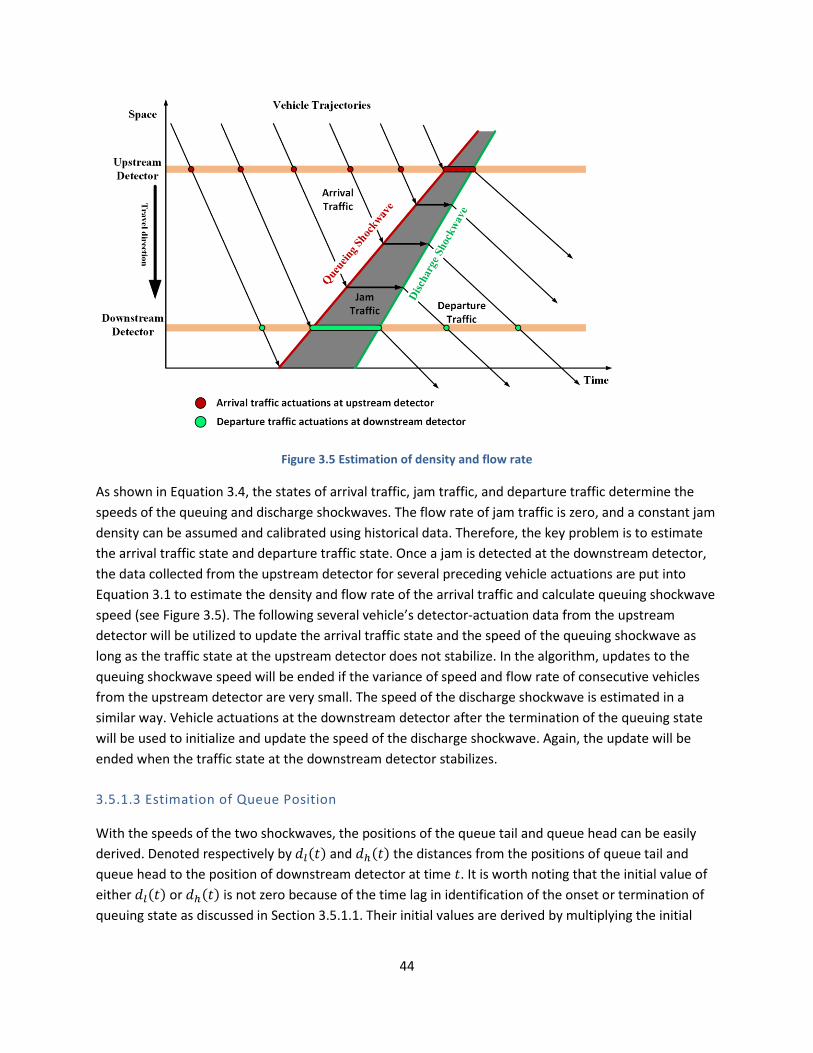
44
Figure 3.5 Estimation of density and flow rate
As shown in Equation 3.4, the states of arrival traffic, jam traffic, and departure traffic determine the
speeds of the queuing and discharge shockwaves. The flow rate of jam traffic is zero, and a constant jam
density can be assumed and calibrated using historical data. Therefore, the key problem is to estimate
the arrival traffic state and departure traffic state. Once a jam is detected at the downstream detector,
the data collected from the upstream detector for several preceding vehicle actuations are put into
Equation 3.1 to estimate the density and flow rate of the arrival traffic and calculate queuing shockwave
speed (see Figure 3.5). The following several vehicle’s detector-actuation data from the upstream
detector will be utilized to update the arrival traffic state and the speed of the queuing shockwave as
long as the traffic state at the upstream detector does not stabilize. In the algorithm, updates to the
queuing shockwave speed will be ended if the variance of speed and flow rate of consecutive vehicles
from the upstream detector are very small. The speed of the discharge shockwave is estimated in a
similar way. Vehicle actuations at the downstream detector after the termination of the queuing state
will be used to initialize and update the speed of the discharge shockwave. Again, the update will be
ended when the traffic state at the downstream detector stabilizes.
3.5.1.3 Estimation of Queue Position
With the speeds of the two shockwaves, the positions of the queue tail and queue head can be easily
derived. Denoted respectively by 𝑑𝑙(𝑡) and 𝑑ℎ(𝑡) the distances from the positions of queue tail and
queue head to the position of downstream detector at time 𝑡. It is worth noting that the initial value of
either 𝑑𝑙(𝑡) or 𝑑ℎ(𝑡) is not zero because of the time lag in identification of the onset or termination of
queuing state as discussed in Section 3.5.1.1. Their initial values are derived by multiplying the initial

45
shockwave speed by a time delay. Afterwards, the positions of the queue tail and queue head will be
calculated step by step. Let 𝜏 denote time interval of each time step, 𝑑𝑙(𝑡) and 𝑑ℎ(𝑡) can be calculated
by the following equations:
𝑑𝑙(𝑡 + 𝜏) = 𝑑𝑙(𝑡) + 𝑤𝑞(𝑡) × 𝜏
𝑑ℎ(𝑡 + 𝜏) = 𝑑ℎ(𝑡) + 𝑤𝑑(𝑡) × 𝜏 (3.5)
where 𝑤𝑞(𝑡) and 𝑤𝑑(𝑡) are the speeds of queuing and discharge shockwaves at time t, respectively.
Following that, the length of the queue at any time, 𝑞𝑙(𝑡), and the duration of the queue at any space,
𝑞𝑡(𝑥), can be easily derived as follows:
𝑞𝑙(𝑡) = 𝑑𝑙(𝑡) − 𝑑ℎ(𝑡)
𝑞𝑡(𝑥) = 𝑡2 − 𝑡1, 𝑤ℎ𝑒𝑟𝑒 𝑑𝑙(𝑡1) = 𝑑ℎ(𝑡2) = 𝑥 (3.6)
As mentioned before, the algorithm will not update shockwave positions beyond the position of the
upstream detector. Moreover, if the discharge shockwave catches up to the queuing shockwave,
meaning that the queue in the segment has been cleared, the current queuing and discharge
shockwaves will be cleared and the update will be stopped, too.
A flowchart of the queue estimation algorithm is shown in Figure 3.6. This algorithm updates all of the
information (downstream traffic state, queue head, queue tail, shockwave speed, etc.) at every time
step in real time.
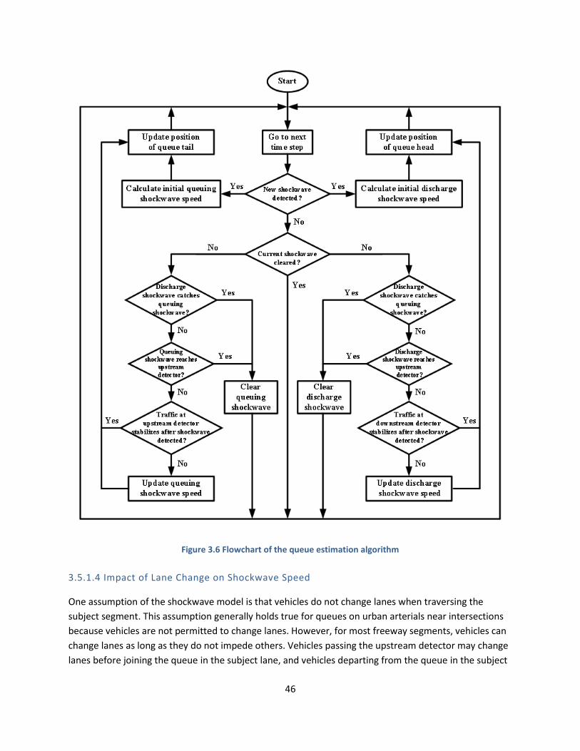
46
Figure 3.6 Flowchart of the queue estimation algorithm
3.5.1.4 Impact of Lane Change on Shockwave Speed
One assumption of the shockwave model is that vehicles do not change lanes when traversing the
subject segment. This assumption generally holds true for queues on urban arterials near intersections
because vehicles are not permitted to change lanes. However, for most freeway segments, vehicles can
change lanes as long as they do not impede others. Vehicles passing the upstream detector may change
lanes before joining the queue in the subject lane, and vehicles departing from the queue in the subject

47
lane may change lanes before showing up at the downstream detector. In this case, using data only from
upstream and downstream detectors in the subject lane to estimate queue may cause non-negligible
errors. To address this problem, a well-recognized lane change model, i.e., the gap acceptance model, is
adopted to modify the original algorithm. Generally, lane changes are executed when drivers are
motivated to do so and safe gaps in both lanes exist. To this end, the traffic states of adjacent lanes are
considered as well. For example, if the subject lane is very congested while the adjacent lanes have less
traffic and safe gaps, drivers from the subject lanes will be motivated to change lanes to avoid
congestion. In the modified algorithm, the differences in the density and speed across lanes are checked
and the number of available gaps that exceed a thresholdsize are counted. Using the information on
density and speed differences and the number of available gaps, the percentage of vehicles changing
lanes can be estimated and used to modify the queuing shockwave speed using the following equation
𝑤𝑞′(𝑡) = 𝑤𝑞(𝑡) × (1 −
𝑛
𝑁)
𝑤𝑑′(𝑡) = 𝑤𝑑(𝑡) × (1 +
𝑛
𝑁)
(3.7)
where 𝑛 is the number of gaps exceed the threshold, and 𝑁 is the number of sampled vehicles.
3.5.1.5 Traffic State Merging for Queuing and Slow-moving States
Unlike the queuing process on urban arterials near intersections, it is sometimes difficult to distinguish
one jam from another on freeway segments. As mentioned before, traffic state changes on freeways do
not have fixed periods or modes. The traffic state can change from stopped queuing to slow-moving and
then quickly go back to the stopped queuing state again. Therefore, it is necessary to merge two or
more consecutive traffic jams into one. This modification is also important in practice because many
active traffic management (ATM) strategies (e.g., warning of stopped traffic) seek to avoid changing
traffic information too frequently.
One example is shown in Figure 3.7(a) shows the case without merge. The times of the start and end of
the first jam are identified as times 𝑡1 and 𝑡2, respectively. The times of the start and end of the second
jam are identified as times 𝑡3 and 𝑡4, respectively. Note that when the second jam is detected at the
downstream detector, the previous jam has not reached the upstream detector. This jam-slow-jam
traffic is likely to become a large jam upstream. In this case, the downstream traffic state between 𝑡2
and 𝑡3 is checked. If the average speed is below a certain threshold 𝑣𝑚, then it will be re-categorized as
jam traffic. This jam-slow-jam traffic is combined into a large jam, as shown in Figure 3.7(b).

48
Figure 3.7 Merge of jam traffic: (a) without merge; (b) with merge
3.5.1.6 Prediction Ability
The ability to predict future traffic states is essential to any queue estimation algorithm. It can help ATM
methods to react in a timely manner. The prediction ability of a queue estimation algorithm is measured
by how early a reliable prediction can be made relative to the time that the real traffic state changes at
the position of interest. In the proposed queue estimation algorithm, although shockwave speed can be
continuously updated after it takes place, it has been found that the speed will converge to a certain
value after five to ten updates. Then a constant shockwave speed can be set and the position of the
head or tail of queue in the near future predicted. The prediction ability of the algorithm depends on the
distance from the location of interest to the downstream detector, the shockwave speed, and the time
needed before the traffic stabilizes.
𝑇𝑝 = 𝑚𝑎𝑥 {𝑥 − 𝑑ℎ(𝑡𝑠)
𝑤, 0} (3.8)
where 𝑇𝑝 is the prediction ability, x is the distance from location of interest to downstream detector, 𝑡𝑠
is the interval from begin of discharge to the time when the traffic stabilizes, and 𝑤 is the stabilized
shockwave speed.
Note that the prediction ability of the proposed algorithm is limited; predictions cannot be made for
locations near the downstream detector.
3.5.2 Field Test of Queue Estimation Algorithm
The proposed algorithm is tested with field data. The data were collected on a 2218-foot-long segment
of I-35W between detector stations S14 and S15. The layout of the loop detectors on I-35W for the
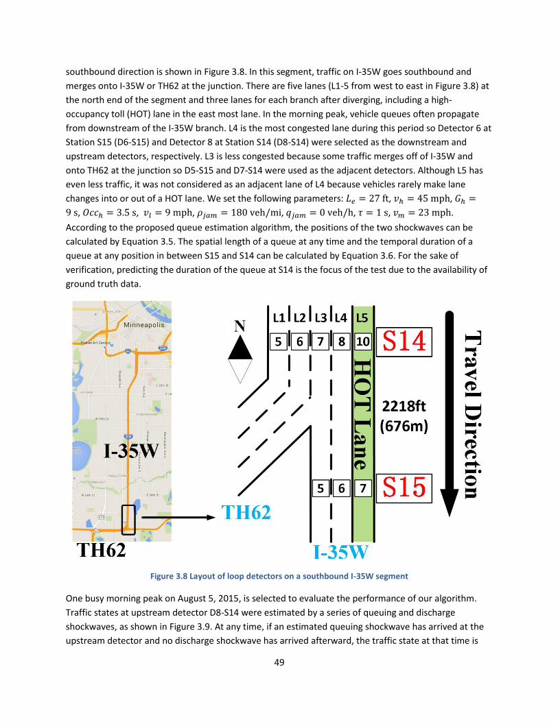
49
southbound direction is shown in Figure 3.8. In this segment, traffic on I-35W goes southbound and
merges onto I-35W or TH62 at the junction. There are five lanes (L1-5 from west to east in Figure 3.8) at
the north end of the segment and three lanes for each branch after diverging, including a high-
occupancy toll (HOT) lane in the east most lane. In the morning peak, vehicle queues often propagate
from downstream of the I-35W branch. L4 is the most congested lane during this period so Detector 6 at
Station S15 (D6-S15) and Detector 8 at Station S14 (D8-S14) were selected as the downstream and
upstream detectors, respectively. L3 is less congested because some traffic merges off of I-35W and
onto TH62 at the junction so D5-S15 and D7-S14 were used as the adjacent detectors. Although L5 has
even less traffic, it was not considered as an adjacent lane of L4 because vehicles rarely make lane
changes into or out of a HOT lane. We set the following parameters: 𝐿𝑒 = 27 ft, 𝑣ℎ = 45 mph, 𝐺ℎ =
9 s, 𝑂𝑐𝑐ℎ = 3.5 s, 𝑣𝑙 = 9 mph, 𝜌𝑗𝑎𝑚 = 180 veh/mi, 𝑞𝑗𝑎𝑚 = 0 veh/h, 𝜏 = 1 s, 𝑣𝑚 = 23 mph.
According to the proposed queue estimation algorithm, the positions of the two shockwaves can be
calculated by Equation 3.5. The spatial length of a queue at any time and the temporal duration of a
queue at any position in between S15 and S14 can be calculated by Equation 3.6. For the sake of
verification, predicting the duration of the queue at S14 is the focus of the test due to the availability of
ground truth data.
Figure 3.8 Layout of loop detectors on a southbound I-35W segment
One busy morning peak on August 5, 2015, is selected to evaluate the performance of our algorithm.
Traffic states at upstream detector D8-S14 were estimated by a series of queuing and discharge
shockwaves, as shown in Figure 3.9. At any time, if an estimated queuing shockwave has arrived at the
upstream detector and no discharge shockwave has arrived afterward, the traffic state at that time is
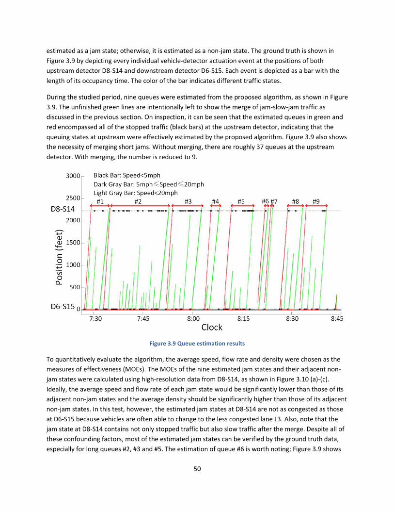
50
estimated as a jam state; otherwise, it is estimated as a non-jam state. The ground truth is shown in
Figure 3.9 by depicting every individual vehicle-detector actuation event at the positions of both
upstream detector D8-S14 and downstream detector D6-S15. Each event is depicted as a bar with the
length of its occupancy time. The color of the bar indicates different traffic states.
During the studied period, nine queues were estimated from the proposed algorithm, as shown in Figure
3.9. The unfinished green lines are intentionally left to show the merge of jam-slow-jam traffic as
discussed in the previous section. On inspection, it can be seen that the estimated queues in green and
red encompassed all of the stopped traffic (black bars) at the upstream detector, indicating that the
queuing states at upstream were effectively estimated by the proposed algorithm. Figure 3.9 also shows
the necessity of merging short jams. Without merging, there are roughly 37 queues at the upstream
detector. With merging, the number is reduced to 9.
Figure 3.9 Queue estimation results
To quantitatively evaluate the algorithm, the average speed, flow rate and density were chosen as the
measures of effectiveness (MOEs). The MOEs of the nine estimated jam states and their adjacent non-
jam states were calculated using high-resolution data from D8-S14, as shown in Figure 3.10 (a)-(c).
Ideally, the average speed and flow rate of each jam state would be significantly lower than those of its
adjacent non-jam states and the average density should be significantly higher than those of its adjacent
non-jam states. In this test, however, the estimated jam states at D8-S14 are not as congested as those
at D6-S15 because vehicles are often able to change to the less congested lane L3. Also, note that the
jam state at D8-S14 contains not only stopped traffic but also slow traffic after the merge. Despite all of
these confounding factors, most of the estimated jam states can be verified by the ground truth data,
especially for long queues #2, #3 and #5. The estimation of queue #6 is worth noting; Figure 3.9 shows
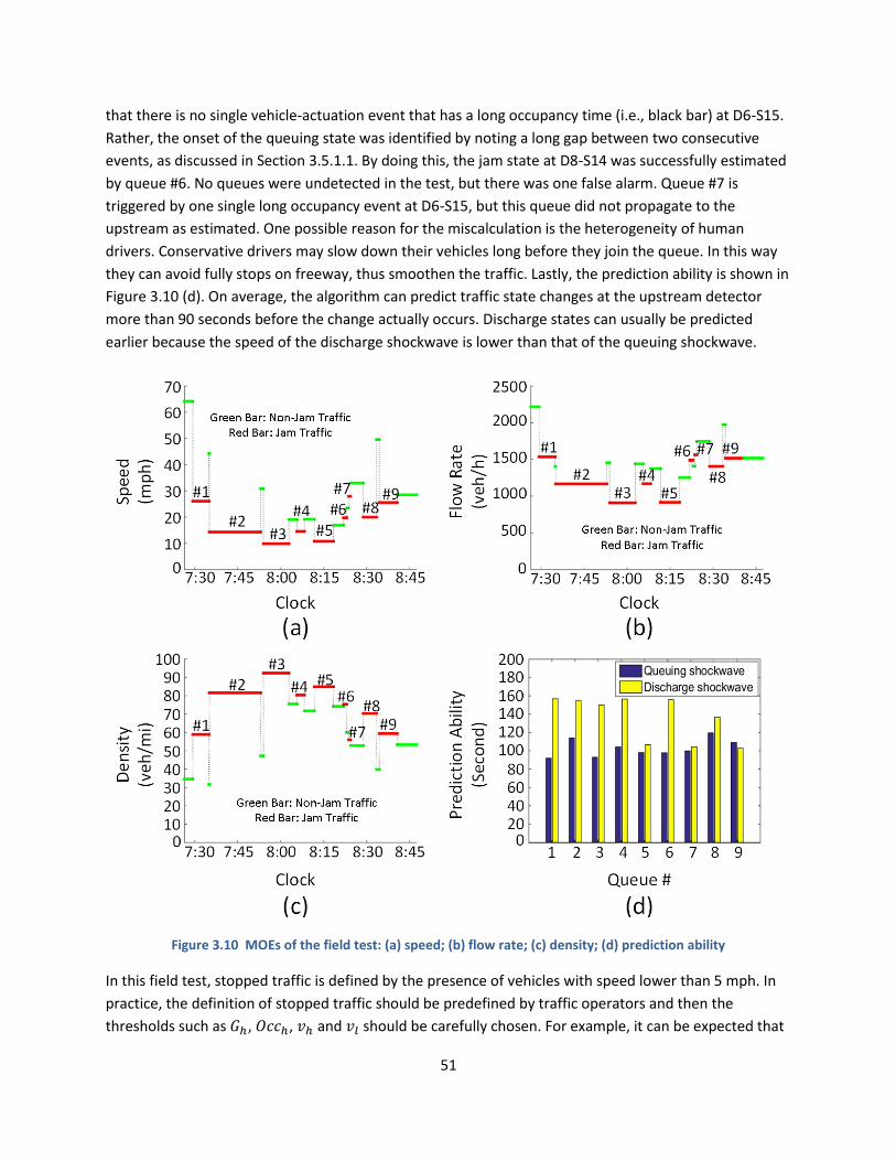
51
that there is no single vehicle-actuation event that has a long occupancy time (i.e., black bar) at D6-S15.
Rather, the onset of the queuing state was identified by noting a long gap between two consecutive
events, as discussed in Section 3.5.1.1. By doing this, the jam state at D8-S14 was successfully estimated
by queue #6. No queues were undetected in the test, but there was one false alarm. Queue #7 is
triggered by one single long occupancy event at D6-S15, but this queue did not propagate to the
upstream as estimated. One possible reason for the miscalculation is the heterogeneity of human
drivers. Conservative drivers may slow down their vehicles long before they join the queue. In this way
they can avoid fully stops on freeway, thus smoothen the traffic. Lastly, the prediction ability is shown in
Figure 3.10 (d). On average, the algorithm can predict traffic state changes at the upstream detector
more than 90 seconds before the change actually occurs. Discharge states can usually be predicted
earlier because the speed of the discharge shockwave is lower than that of the queuing shockwave.
Figure 3.10 MOEs of the field test: (a) speed; (b) flow rate; (c) density; (d) prediction ability
In this field test, stopped traffic is defined by the presence of vehicles with speed lower than 5 mph. In
practice, the definition of stopped traffic should be predefined by traffic operators and then the
thresholds such as 𝐺ℎ, 𝑂𝑐𝑐ℎ, 𝑣ℎ and 𝑣𝑙 should be carefully chosen. For example, it can be expected that
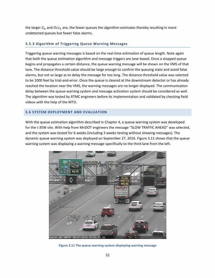
52
the larger 𝐺ℎ and 𝑂𝑐𝑐ℎ are, the fewer queues the algorithm estimates thereby resulting in more
undetected queues but fewer false alarms.
3.5.3 Algorithm of Triggering Queue Warning Messages
Triggering queue warning messages is based on the real-time estimation of queue length. Note again
that both the queue estimation algorithm and message triggers are lane-based. Once a stopped queue
begins and propagates a certain distance, the queue warning message will be shown on the VMS of that
lane. The distance threshold value should be large enough to confirm the queuing state and avoid false
alarms, but not so large as to delay the message for too long. The distance threshold value was selected
to be 1000 feet by trial-and-error. Once the queue is cleared at the downstream detector or has already
reached the location near the VMS, the warning messages are no longer displayed. The communication
delay between the queue warning system and message activation system should be considered as well.
The algorithm was tested by RTMC engineers before its implementation and validated by checking field
videos with the help of the MTO.
3.6 SYSTEM DEPLOYMENT AND EVALUATION
With the queue estimation algorithm described in Chapter 4, a queue warning system was developed
for the I-35W site. With help from MnDOT engineers the message “SLOW TRAFFIC AHEAD” was selected,
and the system was tested for 6 weeks (including 3 weeks testing without showing messages). The
dynamic queue warning system was deployed on September 27, 2016. Figure 3.11 shows that the queue
warning system was displaying a warning message specifically to the third lane from the left.
Figure 3.11 The queue warning system displaying warning message
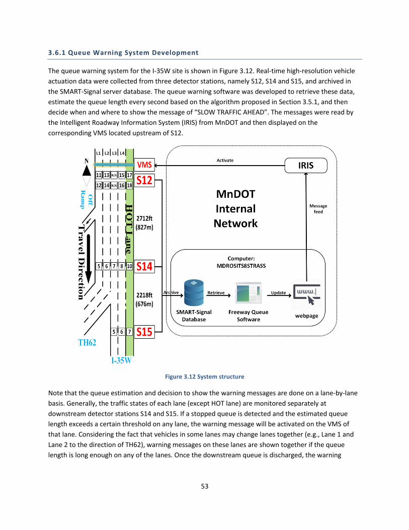
53
3.6.1 Queue Warning System Development
The queue warning system for the I-35W site is shown in Figure 3.12. Real-time high-resolution vehicle
actuation data were collected from three detector stations, namely S12, S14 and S15, and archived in
the SMART-Signal server database. The queue warning software was developed to retrieve these data,
estimate the queue length every second based on the algorithm proposed in Section 3.5.1, and then
decide when and where to show the message of “SLOW TRAFFIC AHEAD”. The messages were read by
the Intelligent Roadway Information System (IRIS) from MnDOT and then displayed on the
corresponding VMS located upstream of S12.
Figure 3.12 System structure
Note that the queue estimation and decision to show the warning messages are done on a lane-by-lane
basis. Generally, the traffic states of each lane (except HOT lane) are monitored separately at
downstream detector stations S14 and S15. If a stopped queue is detected and the estimated queue
length exceeds a certain threshold on any lane, the warning message will be activated on the VMS of
that lane. Considering the fact that vehicles in some lanes may change lanes together (e.g., Lane 1 and
Lane 2 to the direction of TH62), warning messages on these lanes are shown together if the queue
length is long enough on any of the lanes. Once the downstream queue is discharged, the warning
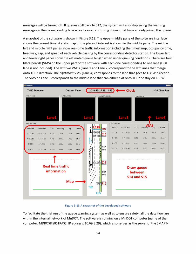
54
messages will be turned off. If queues spill back to S12, the system will also stop giving the warning
message on the corresponding lane so as to avoid confusing drivers that have already joined the queue.
A snapshot of the software is shown in Figure 3.13. The upper middle pane of the software interface
shows the current time. A static map of the place of interest is shown in the middle pane. The middle
left and middle right panes show real-time traffic information including the timestamp, occupancy time,
headway, gap, and speed of each vehicle passing by the corresponding detector station. The lower left
and lower right panes show the estimated queue length when under queuing conditions. There are four
black boards (VMS) on the upper part of the software with each one corresponding to one lane (HOT
lane is not included). The left two VMSs (Lane 1 and Lane 2) correspond to the left lanes that merge
onto TH62 direction. The rightmost VMS (Lane 4) corresponds to the lane that goes to I-35W direction.
The VMS on Lane 3 corresponds to the middle lane that can either exit onto TH62 or stay on I-35W.
Figure 3.13 A snapshot of the developed software
To facilitate the trial run of the queue warning system as well as to ensure safety, all the data flow are
within the internal network of MnDOT. The software is running on a MnDOT computer (name of the
computer: MDROSITS8STRASS; IP address: 10.69.3.29), which also serves as the server of the SMART-
55
Signal system that archives high-resolution traffic data in real time. In MnDOT, the VMS is activated by
IRIS at the request of an external system by using the "msg feed" protocol. Once the developed software
decides to put a message on VMS, it will write the message to a text file. This text file can be reached at
http://10.69.3.29/msgfeed/test.txt within MnDOT’s internal network. IRIS polls this HTTP URL every 30
seconds and updates the VMSs accordingly.
3.6.1.1 Evaluation of Warning Messages
Following the advice of MnDOT, this task evaluates the warning message of “SLOW TRAFFIC AHEAD”.
The data collected for evaluation are mainly from loop detectors. Video data are also used to check the
effectiveness of the system. To compare the results, 3 weeks’ data before the deployment (from
September 6 to September 26, 2016) and 3 weeks’ data after the deployment (from September 28 to
October 18, 2016) were used. A total of 1,176 warning messages were triggered by the queue warning
system for the before case. Note again that those warning messages were not really shown on VMS. A
total of 999 warning messages were triggered by the queue warning system for the after case. Those
warning messages were shown on the VMS. For each message, the period of interest is the period when
the message is turned on plus one minute after the message is turned off. The one-minute post-
message period is also considered because the effect of warning messages extends beyond the time of
deactivation.
3.6.1.2 Hypothesis Testing for Changes Before/After Deployment
Based on the before and after data collected, the mean value and standard deviation of speed were
calculated for each detector and for each message and hypothesis testing was then carried out to see
whether there was significant change before and after the deployment of the system (note that
consecutive messages are combined into one single message in this part). Take the mean speed at
detector station S14 (see Figures 3-15 and 3-16) as an example.
In order to confirm whether the mean speed after deployment is statistically significantly lower than
that before deployment, the following hypothesis test is performed:
Two-sample hypotheses concerning the means:
𝑋1𝑖 = average speed during 𝑖th message, before the deployment;
𝑛1 = number of separate messages, before the deployment (consecutive messages are
combined);
𝑋2𝑗 = average speed during 𝑗th message, after the deployment;
𝑛2 = number of separate messages, after the deployment;
𝛼 = 0.05;

56
Assume 𝑋1𝑖~𝑁(𝜇1, 𝜎12), 𝑋2𝑗~𝑁(𝜇2, 𝜎2
2)
𝐻0: 𝜇1 ≥ 𝜇2, i.e. mean speed does not increase after the deployment.
𝐻1: 𝜇1 < 𝜇2, i.e. mean speed increases after the deployment.
Rejection region: 𝑡𝜐1+𝜐2 ≤ 𝑡𝜐1+𝜐2(𝛼) ;
𝜐1 = 𝑛1 − 1; �̅�1 =1
𝑛1∑ 𝑋1𝑖
𝑛1𝑖=1 ; 𝑠1
2 =1
𝑛1−1∑ (𝑋1𝑖 − �̅�1)2𝑛1
𝑖=1 ;
𝜐2 = 𝑛2 − 1; �̅�2 =1
𝑛2∑ 𝑋2𝑗
𝑛2𝑗=1 ; 𝑠2
2 =1
𝑛2−1∑ (𝑋2𝑗 − �̅�2)2𝑛2
𝑗=1 ;
𝑆𝑝2 = √
(𝑛1−1)𝑠12+(𝑛2−1)𝑠2
2
𝑛1+𝑛2−2;
𝑡𝜐1+𝜐2 =�̅�1 − �̅�2
√𝑆𝑝
2
𝑛1+
𝑆𝑝2
𝑛2
.
The results are shown in the Table 3-3.
Table 3-3 Hypothesis test (test hypothesis that mean speed at S14 remains the same)
𝒏𝟏 𝒏𝟐 𝒕𝝊𝟏+𝝊𝟐 𝒕𝝊𝟏+𝝊𝟐(𝜶) Conclusion p-value
S14 – Lane 1 160 142 2.6768 -1.6499 Accept 𝐻0 0.9961
S14 – Lane 2 160 142 0.1257 -1.6499 Accept 𝐻0 0.5500
S14 – Lane 3 217 181 -2.1832 -1.6487 Reject 𝐻0 0.0148
S14 – Lane 4 59 60 0.6246 -1.6580 Accept 𝐻0 0.7333
With a confidence level of α = 0.05, it is concluded that the null hypothesis (H0) that the mean speed on
Lane 3 at S14 does not increase after the deployment should be rejected. Therefore, the speed on Lane
3 at S14 after the deployment is significantly higher than that before deployment. For other lanes, there
is no evidence that the speed increases.
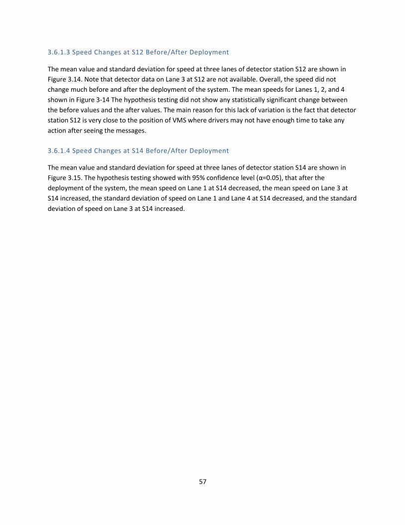
57
3.6.1.3 Speed Changes at S12 Before/After Deployment
The mean value and standard deviation for speed at three lanes of detector station S12 are shown in
Figure 3.14. Note that detector data on Lane 3 at S12 are not available. Overall, the speed did not
change much before and after the deployment of the system. The mean speeds for Lanes 1, 2, and 4
shown in Figure 3-14 The hypothesis testing did not show any statistically significant change between
the before values and the after values. The main reason for this lack of variation is the fact that detector
station S12 is very close to the position of VMS where drivers may not have enough time to take any
action after seeing the messages.
3.6.1.4 Speed Changes at S14 Before/After Deployment
The mean value and standard deviation for speed at three lanes of detector station S14 are shown in
Figure 3.15. The hypothesis testing showed with 95% confidence level (α=0.05), that after the
deployment of the system, the mean speed on Lane 1 at S14 decreased, the mean speed on Lane 3 at
S14 increased, the standard deviation of speed on Lane 1 and Lane 4 at S14 decreased, and the standard
deviation of speed on Lane 3 at S14 increased.
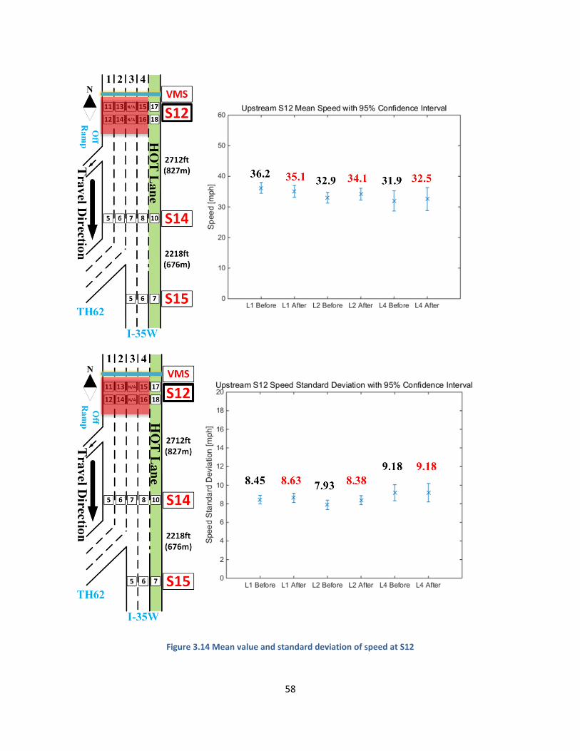
58
Figure 3.14 Mean value and standard deviation of speed at S12
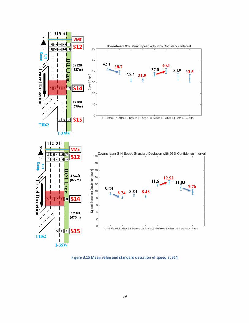
59
Figure 3.15 Mean value and standard deviation of speed at S14
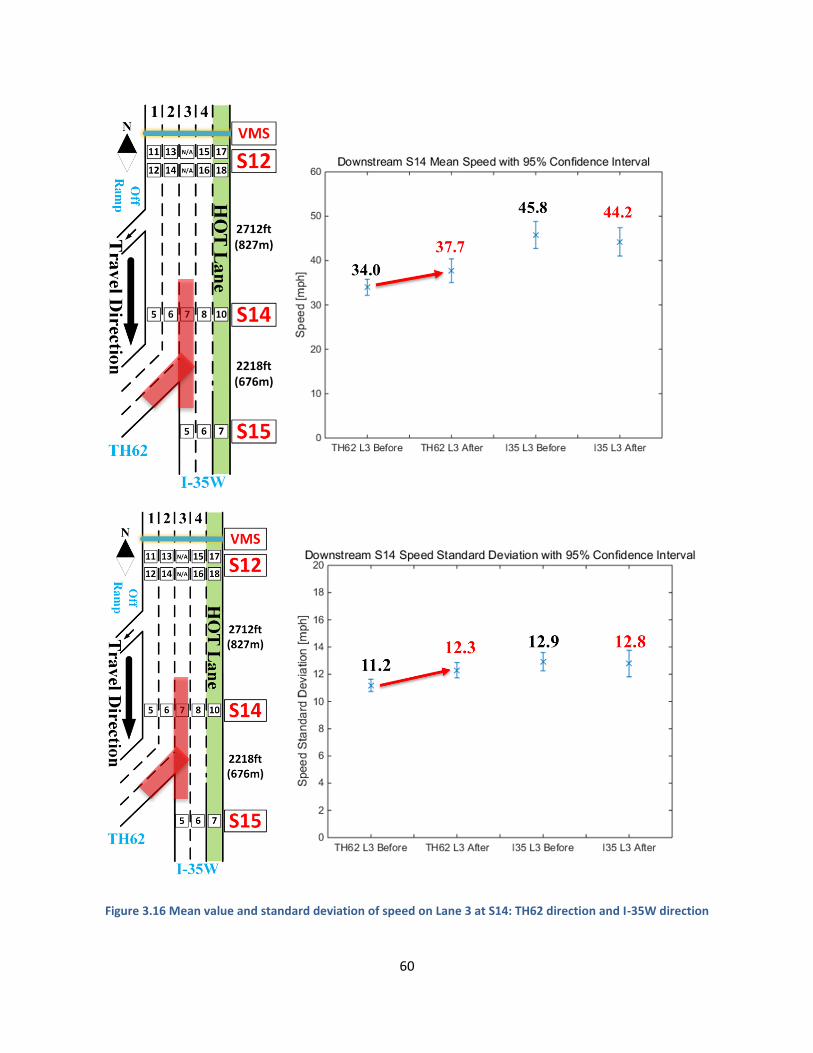
60
Figure 3.16 Mean value and standard deviation of speed on Lane 3 at S14: TH62 direction and I-35W direction
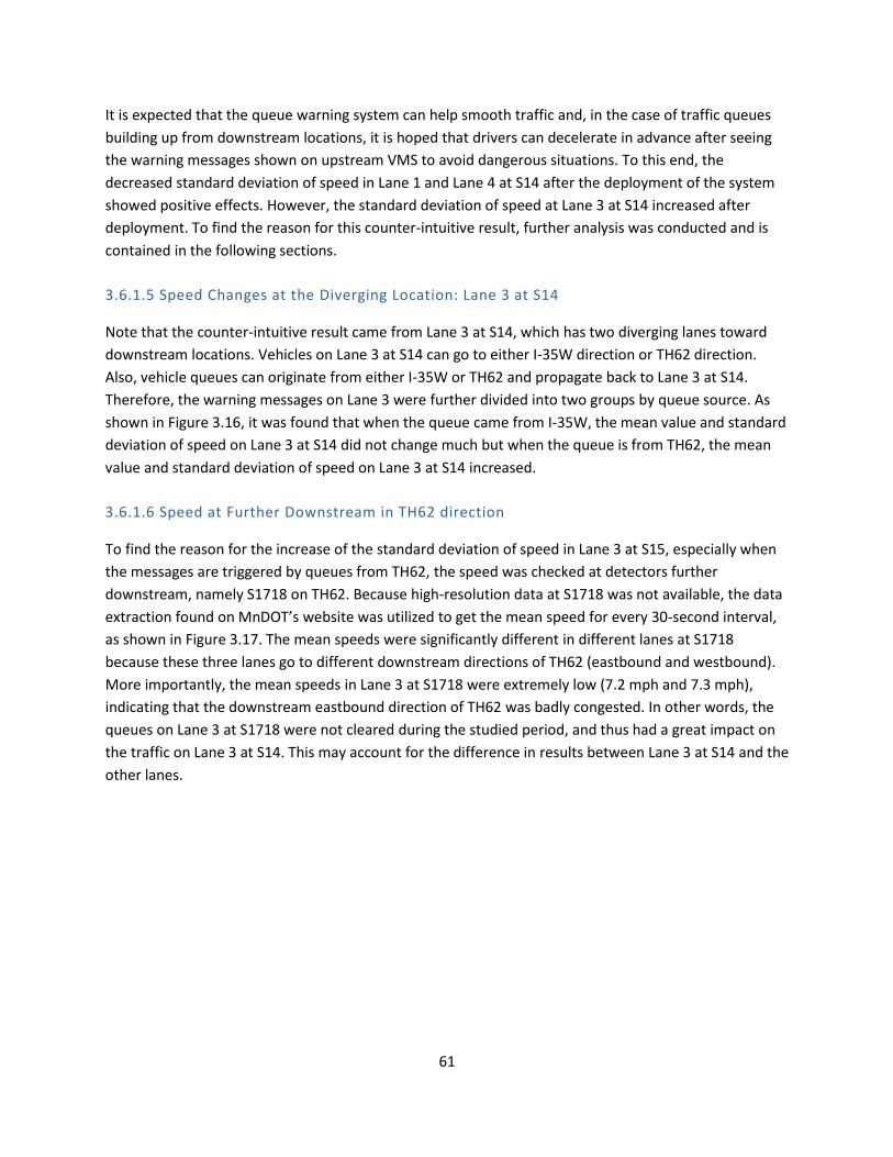
61
It is expected that the queue warning system can help smooth traffic and, in the case of traffic queues
building up from downstream locations, it is hoped that drivers can decelerate in advance after seeing
the warning messages shown on upstream VMS to avoid dangerous situations. To this end, the
decreased standard deviation of speed in Lane 1 and Lane 4 at S14 after the deployment of the system
showed positive effects. However, the standard deviation of speed at Lane 3 at S14 increased after
deployment. To find the reason for this counter-intuitive result, further analysis was conducted and is
contained in the following sections.
3.6.1.5 Speed Changes at the Diverging Location: Lane 3 at S14
Note that the counter-intuitive result came from Lane 3 at S14, which has two diverging lanes toward
downstream locations. Vehicles on Lane 3 at S14 can go to either I-35W direction or TH62 direction.
Also, vehicle queues can originate from either I-35W or TH62 and propagate back to Lane 3 at S14.
Therefore, the warning messages on Lane 3 were further divided into two groups by queue source. As
shown in Figure 3.16, it was found that when the queue came from I-35W, the mean value and standard
deviation of speed on Lane 3 at S14 did not change much but when the queue is from TH62, the mean
value and standard deviation of speed on Lane 3 at S14 increased.
3.6.1.6 Speed at Further Downstream in TH62 direction
To find the reason for the increase of the standard deviation of speed in Lane 3 at S15, especially when
the messages are triggered by queues from TH62, the speed was checked at detectors further
downstream, namely S1718 on TH62. Because high-resolution data at S1718 was not available, the data
extraction found on MnDOT’s website was utilized to get the mean speed for every 30-second interval,
as shown in Figure 3.17. The mean speeds were significantly different in different lanes at S1718
because these three lanes go to different downstream directions of TH62 (eastbound and westbound).
More importantly, the mean speeds in Lane 3 at S1718 were extremely low (7.2 mph and 7.3 mph),
indicating that the downstream eastbound direction of TH62 was badly congested. In other words, the
queues on Lane 3 at S1718 were not cleared during the studied period, and thus had a great impact on
the traffic on Lane 3 at S14. This may account for the difference in results between Lane 3 at S14 and the
other lanes.
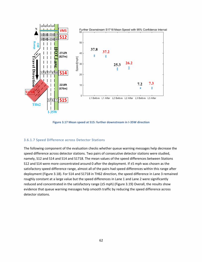
62
Figure 3.17 Mean speed at S15: further downstream in I-35W direction
3.6.1.7 Speed Difference across Detector Stations
The following component of the evaluation checks whether queue warning messages help decrease the
speed difference across detector stations. Two pairs of consecutive detector stations were studied,
namely, S12 and S14 and S14 and S1718. The mean values of the speed differences between Stations
S12 and S14 were more concentrated around 0 after the deployment. If ±5 mph was chosen as the
satisfactory speed difference range, almost all of the pairs had speed differences within this range after
deployment (Figure 3.18). For S14 and S1718 in TH62 direction, the speed difference in Lane 3 remained
roughly constant at a large value but the speed differences in Lane 1 and Lane 2 were significantly
reduced and concentrated in the satisfactory range (±5 mph) (Figure 3.19) Overall, the results show
evidence that queue warning messages help smooth traffic by reducing the speed difference across
detector stations.
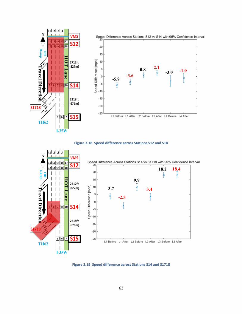
63
Figure 3.18 Speed difference across Stations S12 and S14
Figure 3.19 Speed difference across Stations S14 and S1718
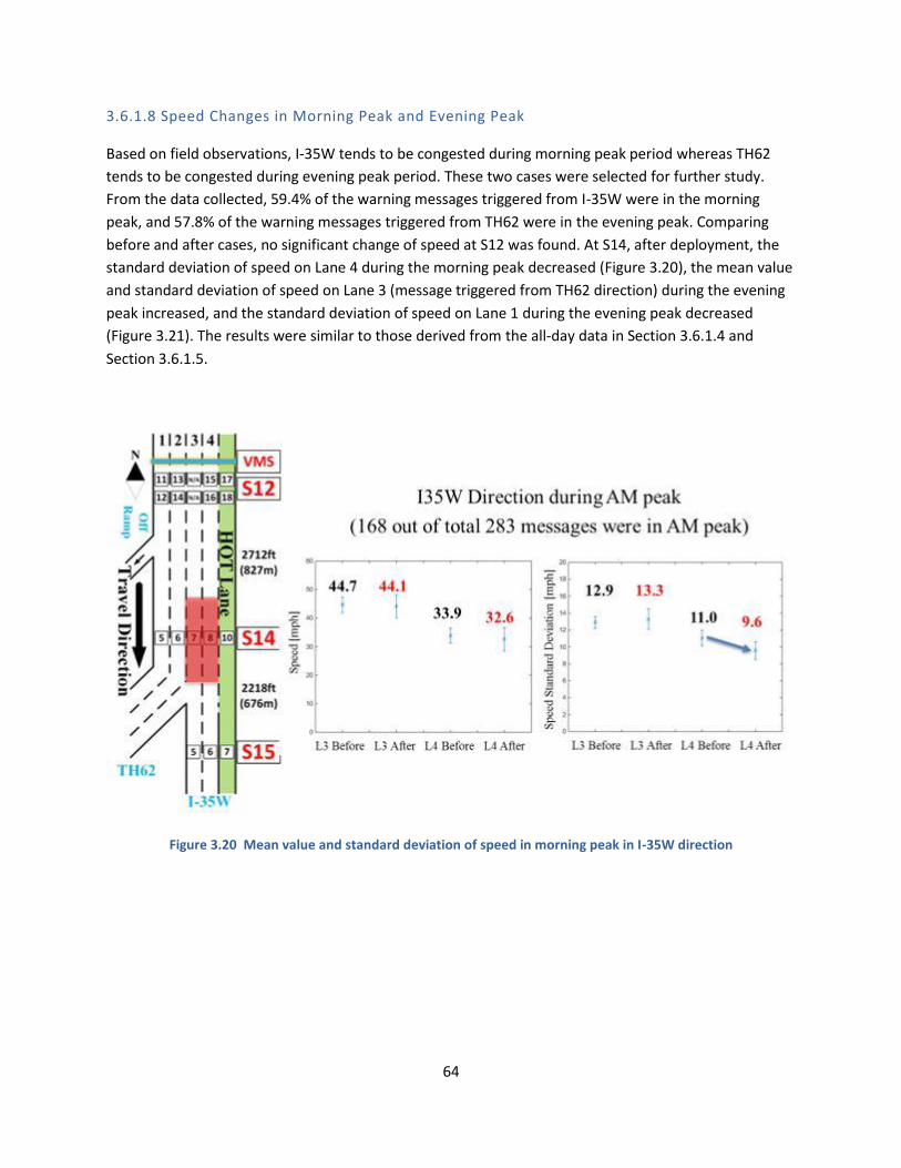
64
3.6.1.8 Speed Changes in Morning Peak and Evening Peak
Based on field observations, I-35W tends to be congested during morning peak period whereas TH62
tends to be congested during evening peak period. These two cases were selected for further study.
From the data collected, 59.4% of the warning messages triggered from I-35W were in the morning
peak, and 57.8% of the warning messages triggered from TH62 were in the evening peak. Comparing
before and after cases, no significant change of speed at S12 was found. At S14, after deployment, the
standard deviation of speed on Lane 4 during the morning peak decreased (Figure 3.20), the mean value
and standard deviation of speed on Lane 3 (message triggered from TH62 direction) during the evening
peak increased, and the standard deviation of speed on Lane 1 during the evening peak decreased
(Figure 3.21). The results were similar to those derived from the all-day data in Section 3.6.1.4 and
Section 3.6.1.5.
Figure 3.20 Mean value and standard deviation of speed in morning peak in I-35W direction
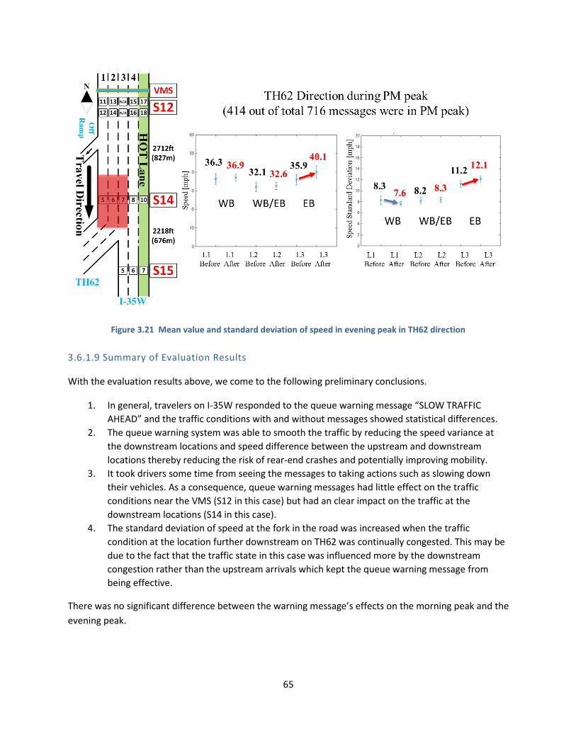
65
Figure 3.21 Mean value and standard deviation of speed in evening peak in TH62 direction
3.6.1.9 Summary of Evaluation Results
With the evaluation results above, we come to the following preliminary conclusions.
1. In general, travelers on I-35W responded to the queue warning message “SLOW TRAFFIC
AHEAD” and the traffic conditions with and without messages showed statistical differences.
2. The queue warning system was able to smooth the traffic by reducing the speed variance at
the downstream locations and speed difference between the upstream and downstream
locations thereby reducing the risk of rear-end crashes and potentially improving mobility.
3. It took drivers some time from seeing the messages to taking actions such as slowing down
their vehicles. As a consequence, queue warning messages had little effect on the traffic
conditions near the VMS (S12 in this case) but had an clear impact on the traffic at the
downstream locations (S14 in this case).
4. The standard deviation of speed at the fork in the road was increased when the traffic
condition at the location further downstream on TH62 was continually congested. This may be
due to the fact that the traffic state in this case was influenced more by the downstream
congestion rather than the upstream arrivals which kept the queue warning message from
being effective.
There was no significant difference between the warning message’s effects on the morning peak and the
evening peak.
66
3.7 DISCUSSION
Rear-end crashes are the most frequent type of crashes observed on freeways and research has shown
that freeway rear-end crashes tend to occur in extended congested traffic situations where the speed
variation is large, e.g. end-of-queue locations. One of the prevailing active traffic management strategies
is the ILCS system that displays messages to warn drivers about upcoming queues and caution them to
adjust their speed to avoid potential rear-end collisions. One main component of such active traffic
management strategies is the real-time queue estimation algorithm which depends highly on the data
being utilized.
In this project, a real-time queue warning system was developed and deployed on a freeway segment on
I-35W south of Minneapolis, MN. Benefiting from a previously-developed data collection system , five
sets of data collection devices were installed on the segment of interest. High-resolution detector
actuation data were then collected from the field. By taking advantage of such high-resolution event-
based data, every traffic state change at detector locations can be identified within a few seconds.
Shockwave analysis is adopted to develop the real-time queue estimation algorithm. The algorithm runs
locally in any freeway segment between an upstream detector and a downstream detector, estimating
the length and duration of a queue once the queue is detected by the downstream detector. When the
queue extends upstream of the upstream detector, the algorithm stops estimating it with further
estimation of the queue being provided by the same algorithm running in the next segment upstream.
Due to the differences in traffic states between lanes (e.g., lanes to different directions of a diverge
junction), one instance of the algorithm runs for each lane. The impact of lane changes is considered as
well by analyzing traffic data from detectors on adjacent lanes. The algorithm also has limited capability
of prediction as to the time when a queue will be formed or cleared at any position in this segment nor
can it predict the queue length in this segment at any time in the near future. The proposed algorithm
was tested with field data and validated by video captured in the field.
The queue warning system was tested in the field for three weeks, showing the queue warning message
“SLOW TRAFFIC AHEAD” to travelers when a queue was estimated at downstream locations. Before
that, the system had also been running for three weeks without actually showing messages. The high-
resolution data from loop detectors, the queue warning system log files archiving the start time,
duration, and location of triggered messages (including those not shown on VMS before field test), and
videos from MnDOT cameras were used to evaluate the queue warning system. By comparing the
before and after cases, the impacts of warning messages were studied. Promisingly, for most of the
studied locations, the study showed that queue warning messages helped to reduce the speed variance
near the queue locations and the speed difference between upstream and downstream locations. This
also implies a satisfactory level of compliance rate by drivers.
67
CONCLUDING REMARKS
The research described in this report is aimed at developing and field-testing two queue warning
systems following different philosophies in regard to rear-end collision safety. The MQWA system
philosophy follows the premise that freeway rear-end collisions tend to occur in extended stop-and-go
traffic or at end-of-queue locations. The MQWA system prototype was deployed and evaluated in
Minneapolis, MN, on I-35W southbound where conditions supported this hypothesis. QWARN is based
on the hypothesis that not all congestion events are dangerous and that certain traffic conditions that
are crash prone regardless of whether they result in standing queues or not. Such CPCs can be isolated,
fast moving shockwaves, involving only a small number of vehicles in the deceleration-stop-acceleration
cycle. One location where such conditions have been identified and result in more than 100 crashes per
year is the westbound section of I-94 in downtown Minneapolis, MN. This location was selected for the
QWARN deployment and evaluation.
Although, each system was evaluated using different methodologies, both have demonstrated a positive
effect on driver behavior. The MQWA system on I-35W has smoothed the traffic flow by reducing the
speed variance at downstream locations and speed difference between upstream and downstream. The
evaluation period (three weeks) was short so no data on the actual influence of the system on crash
rates were collected. QWARN’s deployment on I-94 has resulted in a 22% reduction in crashes and a
54% reduction in near-crash events during a three-month evaluation period. In both cases, the short
evaluation periods can only show promise and longer traffic safety studies are needed to show whether
the systems will have a lasting effect on safety in their respective corridors. Following the reporting of
the evaluation results, MnDOT has lifted the restriction that the system only operate between noon and
8 p.m. and now allows the alarms to be displayed any time the system detects a crash-prone condition.
At the time this report was written, both systems were in operation. Although, there are no current
plans to expand the deployment of the MQWA system, MnDOT expressed the desire to deploy QWARN
in two upstream locations on the I-94 WB corridor in anticipation of CPCs following the beginning of
construction on the stretch of I-94 QWARN is currently deployed on. Although funding has not been
secured yet for such an expansion, the Minnesota Traffic Observatory is continuing to refine QWARN as
well as the collect video and detector data to facilitate a longer-term evaluation.
68
REFERENCES
1. Early Estimate of Motor Vehicle Traffic Fatalities in 2014,
https://crashstats.nhtsa.dot.gov/Api/Public/ViewPublication/812160
2. Benefit-Cost Analysis for Transportation Projects,
http://www.dot.state.mn.us/planning/program/appendix_a.html
3. Minnesota Traffic Crashes in 2014, https://dps.mn.gov/divisions/ots/reports-
statistics/Documents/2014-crash-facts.pdf https://dps.mn.gov/divisions/ots/reports-
statistics/Documents/2014-crash-facts.pdf
4. Hourdos, J., Garg, V., Michalopoulos, P., & Davis, G. (2006). Real-Time Detection of Crash-Prone
Conditions at Freeway High-Crash Locations. Transportation Research Record, 1968(1), 83–91.
doi: 10.3141/1968-10
5. Qiu, L., & Nixon, W. A. (2008). Effects of Adverse Weather on Traffic Crashes: Systematic Review
and Meta-Analysis. Transportation Research Record, 2055, 139–146. doi:10.3141/2055-16
6. Kopelias, P., Papadimitriou, F., Papandreou, K., & Prevedouros, P. (2007). Urban Freeway Crash
Analysis: Geometric, Operational, and Weather Effects on Crash Number and Severity.
Transportation Research Record, 2015, 123–131. doi:10.3141/2015-14
7. Golob, T. F., & Recker, W. W. (2003). Relationships Among Urban Freeway Accidents, Traffic
Flow, Weather, and Lighting Conditions. Journal of Transportation Engineering, 129(August),
342–353. doi:10.1061/(ASCE)0733-947X (2003)129:4(342)
8. Zheng, Z., Ahn, S., & Monsere, C. M. (2010). Impact of traffic oscillations on freeway crash
occurrences. Accident Analysis and Prevention, 42(2), 626–636. doi: 10.1016/j.aap.2009.10.009
9. Abdel-Aty, M., Uddin, N., Pande, A., Abdalla, F., & Hsia, L. (2004). Predicting Freeway Crashes
from Loop Detector Data by Matched Case-Control Logistic Regression. Transportation Research
Record.
10. Caliendo, C., Guida, M., & Parisi, A. (2007). A crash-prediction model for multilane roads.
Accident Analysis and Prevention, 39(4), 657–670. doi: 10.1016/ j.aap. 2006.10.012
11. Pei, X., Wong, S. C., & Sze, N. N. (2011). A joint-probability approach to crash prediction models.
Accident Analysis and Prevention, 43(3), 1160–1166. doi: 10.1016/ j.aap. 2010.12.026
12. Naderan, A., & Shahi, J. (2010). Aggregate crash prediction models: Introducing crash generation
concept. Accident Analysis and Prevention, 42(1), 339–346. doi: 10.1016/ j.aap. 2009.08.020
13. Montella, A., Colantuoni, L., & Lamberti, R. (2008). Crash Prediction Models for Rural
Motorways. Transportation Research Record, 2083, 180–189. doi:10.3141/2083-21
69
14. Abdel-Aty, M. A., & Pemmanaboina, R. (2006). Calibrating a real-time traffic crash-prediction
model using archived weather and ITS traffic data. IEEE Transactions on Intelligent
Transportation Systems, 7(2), 167–174.
15. Abdel-Aty, M., & Gayah, V. (2010). Real-Time Crash Risk Reduction on Freeways Using
Coordinated and Uncoordinated Ramp Metering Approaches. Journal of Transportation
Engineering.
16. Lee, C., Hellinga, B., & Saccomanno, F. (2003). Real-Time Crash Prediction Model for Application
to Crash Prevention in Freeway Traffic. Transportation Research Record, 1840, 67–77.
doi:10.3141/1840-08
17. Khan, A. Intelligent infrastructure-based queue-end warning system for avoiding rear impacts.
IET Intelligent Transportation Systems, Vol. 1, No. 2, 2007, p. 138.
18. ARTBA Work Zone Safety Consortium. Innovative End-of Queue Warning System Reduces
Crashes Up to 45%. ARTBA Work Zone Safety Consortium, 2015.
19. Pesti, G., P. Wiles, R. Cheu, P. Songchitruska, J. Shelton, and S. Cooner. (2007) Traffic Control
Strategies for Congested Freeways and Work Zones. Texas Department of Transportation.
20. Delta Highway Queue Warning System Evaluation - Final Technical Memorandum.
http://www.kittelson.com/projects/intelligent-transportation-systems-its-statewide-
evaluations. Accessed Jul. 19, 2016.
21. Mahmassani, H., Rakha, H., Hubbard, E., and Lukasik, D. Concept Development and Needs
Identification for Intelligent Network Flow Optimization (INFLO). USDOT ITS Joint Program
Office, 2012.
22. Hourdakis, J., Michalopoulos, P. G., and Morris, T. (2004) Deployment of Wireless Mobile
Detection and Surveillance for Data-Intensive Applications. In Transportation Research Record,
pp. 140–148.
23. Jones, T., and Potts R. "The Measurement of Acceleration Noise-A Traffic Parameter."
Operations Research 10.6 (1962): 745-63. Web.
24. Helly, W., and Baker, P.G., (1965). “Acceleration noise in a congested signalized environment.”
Vehicular Traffic Science. Proceedings of the Third International Symposium on the Theory of
Traffic Flow. pp. 55-61.
25. Greenshields, B. D. (1961) “Quality of Traffic Flow, Quality and Theory of Traffic Flow.”
Symposium, Bureau of Highway Traffic, Yale University, New Haven, Conn. pp.3-40.
26. Phillips, W. F., (1979). “A kinetic model for traffic flow with continuum implications”.
Transportation Planning and Technology 5, 131-138.
70
27. Drew, D., (1968) Traffic Flow Control and Theory, McGraw Hill.
28. Hourdos, J. (2005) Crash prone traffic flow dynamics: Identification and real-time detection.
Ph.D. dissertation, University of Minnesota, 315 pages.
29. Pande, A. and Abdel-Aty, M. (2006) Assessment of freeway traffic parameters leading to lane-
change related collisions, Accident Analysis & Prevention, 38, (5), p. 936-948
30. Akcelik, R. (1998), A queue model for HCM 2000, ARRB Transportation Research Ltd., Vermont
South, Australia.
31. Balke, K., Charara, H. and Parker, R. (2005), Development of a traffic signal performance
measurement system (TSPMS), Texas Transportation Institute, The Texas A&M University
System College Station, TX.
32. Bertini, R.L., Boice, S. and Bogenberger, K. (2006), Dynamics of Variable Speed Limit System
Surrounding Bottleneck on German Autobahn, Transportation Research Record, no. 1978, pp.
149-159.
33. Catling, I. (1977), A time dependent approach to junction delays, Traffic Engineering and
Control, 18, (11), pp. 520-526.
34. Chan, C. (2012), Monitoring and Improving Roadway Surface Conditions For Safe Driving
Environment and Sustainable Infrastructure, University of California Berkeley – PATH, Richmond
Field Station, Bldg., Richmond, CA.
35. Chang, T. and Lin, J. 2000, "Optimal signal timing for an oversaturated intersection",
Transportation Research Part B: Methodological, 34, (6), 471-491.
36. Chatterjee, K., Hounsell, N.B., Firmin, P.E. and Bonsall, P.W. (2002), Driver response to variable
message sign information in London, Transportation Research Part C: Emerging Technologies,
10, (2), 149-169.
37. Cheng, Y., Qin, X., Jin, J. and Ran, B. (2012), An Exploratory Shockwave Approach to Estimating
Queue Length Using Probe Trajectories, Journal of intelligent transportation systems, 16, (1), 12-
23.
38. Comert, G. and Cetin, M. (2009), Queue length estimation from probe vehicle location and the
impacts of sample size, European Journal of Operational Research, 197, (1), 196-202.
39. Cronje, W.B. (1983a), Analysis of existing formulas for delay, overflow, and stops, Transportation
Research Record, 905, 89-93.
40. Cronje, W.B. (1983b), Derivation of equations for queue length, stops, and delay for fixed-cycle
traffic signals, Transportation Research Record, 905, 93-95.
71
41. Elefteriadou, L., R. P. Roess and W. R. McShane, (1995). Probabilistic Nature of Breakdown at
Freeway Merge Junctions. Transportation Research Record, 1484, 80-89.
42. Gazis, D.C. (1964), Optimum Control of a System of Oversaturated Intersections, Operations
Research, 12 (6), 815-831.
43. Gazis, D.C. 1974, Traffic Science, New York, N.Y. Wiley-Interscience, Inc.
44. Ghosh-Dastidar, S. and Adeli, H. (2006), Neural Network-Wavelet Microsimulation Model for
Delay and Queue Length Estimation at Freeway Work Zones, Journal of Transportation
Engineering, 132 (4), 331-341.
45. Green, D.H. (1967), Control of Oversaturated Intersections, Operations research, 18 (2), 161-
173.
46. Gregory, C. (2004), Managing Traffic During Poor Visibility "A Journey Through the Fog".
National Highway Visibility Conference (NHVC 2004), Madison, Wisconsin.
47. Harder, K. and Bloomfield, J. (August 2012), Investigating the Effectiveness of Intelligent Lane
Control Signals on Driver Behavior, Minneapolis, MN, Center for Design in Health, College of
Design, University of Minnesota.
48. Hassan, H.M., Abdel-Aty, M., Choi, K. and Algadhi, S.A. (2012), "Driver Behavior and Preferences
for Changeable Message Signs and Variable Speed Limits in Reduced Visibility Conditions",
Journal of Intelligent Transportation Systems, 16 (3), 132-146.
49. Hiribarren, G. and Herrera, J.C. (2014), Real time traffic states estimation on arterials based on
trajectory data, Transportation Research Part B: Methodological, 69 (0), 19-30.
50. Hourdos, J., Garg, V. and Michalopoulos, P.G. (September 2008a), Accident Prevention Based on
Automatic Detection of Accident Prone Traffic Conditions: Phase I, Minneapolis, MN: Intelligent
Transportation Systems Institute, Center for Transportation Studies, University of Minnesota.
51. Hourdos, J., Xin, W. and Michalopoulos, P.G. (December 2008b), Development of Real-Time
Traffic Adaptive Crash Reduction Measures for the Westbound I-94/35W Commons Section,
Minneapolis, MN: Intelligent Transportation Systems Institute, Center for Transportation
Studies, University of Minnesota.
52. Jiang, Y. (2001), A model for estimating traffic delays and vehicle queues at freeway work zones,
Journal of the Transportation Research Forum, 40 (4), 65-81.
53. Karim, A. and Adeli, H. (2003), "Radial Basis Function Neural Network for Work Zone Capacity
and Queue Estimation", Journal of Transportation Engineering, 129 (5), 494-503.
72
54. Khan, A.M. (2007), Intelligent infrastructure-based queue-end warning system for avoiding rear
impacts, Intelligent Transport Systems, IET, 1 (2), 138-143.
55. Lee, C. and Abdel-Aty, M. (2008), Testing Effects of Warning Messages and Variable Speed Limits
on Driver Behavior Using Driving Simulator, Transportation Research Record, 2069 (-1), 55-64.
56. Lighthill, M.J. and Whitham, G.B. (1955), On Kinematic Waves. II. A Theory of Traffic Flow on
Long Crowded Roads, Proceedings of the Royal Society of London A: Mathematical, Physical and
Engineering Sciences, 229 (1178), 317-345.
57. Liu, H.X. and Ma, W. (2009), A virtual vehicle probe model for time-dependent travel time
estimation on signalized arterials, Transportation Research Part C: Emerging Technologies, 17
(1), 11-26.
58. Liu, H.X., Wu, X., Ma, W. and Hu, H. (2009), Real-time queue length estimation for congested
signalized intersections, Transportation Research Part C: Emerging Technologies, 17 (4), 412-
427.
59. MacCarley, C.A. (2005a), Methods and Metrics for Evaluation of an Automated Real-Time Driver
Warning System, Transportation Research Record, 1937, 87-95.
60. MacCarley, C.A. (2005b), Evaluation of Traffic Safety Influence Based on Historical Collision data.
61. Maerivoet, S. and De Moor, B. 2005, "Traffic Flow Theory".
62. Michalopoulos, P.G. and Stephanopoulos, G. (1977a), Oversaturated signal systems with queue
length constraints—I: Single intersection, Transportation Research, 11 (6), 413-421.
63. Michalopoulos, P.G. and Stephanopoulos, G. (1977b), Oversaturated signal systems with queue
length constraints—II: Systems of intersections, Transportation Research, 11 (6), 423-428.
64. Michalopoulos, P. and Stephanopoulos, G. (1981), An application of shock wave theory to traffic
signal control, Transportation Research Part B: Methodological, 15 (1), 35-51.
65. Mirchandani, P.B. and Zou, N. (2007), Queuing Models for Analysis of Traffic Adaptive Signal
Control, Intelligent Transportation Systems, IEEE Transactions, 8 (1), 50-59.
66. Newell, G.F. (1965), Approximation Methods for Queues with Application to the Fixed-Cycle
traffic Light, SIAM Review, 7 (2), 223-240.
67. Richards, P.I. (1956), Shock Waves on the Highway, Operations Research, 4 (1), 42-51.
68. Robertson, D.I. (1969), TRANSY: A traffic network study tool, Road Research Laboratory,
Crowthorne.
73
69. Rouphail, N.M., Courage, K.G. and Strong, D.W. (2006), New Calculation Method for Existing and
Extended Highway Capacity Manual Delay Estimation Procedures, Transportation Research
Board 85th Annual Meeting, Washington, DC.
70. Sharma, A., Bullock, D.M. and Bonneson, J.A. (2007), Input–Output and Hybrid Techniques for
Real-Time Prediction of Delay and Maximum Queue Length at Signalized Intersections,
Transportation Research Record, 2035, 69-80.
71. Sheu, J., Chou, Y. and Shen, L. (2001), A stochastic estimation approach to real-time prediction
of incident effects on freeway traffic congestion, Transportation Research Part B:
Methodological, 35 (6), 575-592.
72. Skabardonis, A. and Geroliminis, N. (2008), "Real-time Monitoring and Control on Signalized
Arterials", Journal of Intelligent Transportation Systems, 12 (2), 64-74.
73. Transportation Research Board 2010, Highway Capacity Manual 2000.
74. Vigos, G., Papageorgiou, M. and Wang, Y. (2008), Real-time estimation of vehicle-count within
signalized links, Transportation Research Part C: Emerging Technologies, 16 (1), 18-35.
75. Webster, F.V. (1958), Traffic Signal Settings, Road Research Technical Paper, vol. 39.
76. Webster, F.V. and Cobbe, B.M. 1966, Traffic signals, H.M.S.O., London.
77. Weng, J. and Meng, Q. (2013), Estimating capacity and traffic delay in work zones: An overview,
Transportation Research Part C: Emerging Technologies, 35, 34-45.
78. Wrapson, W., Harré, N. and Murrell, P. (2006), Reductions in driver speed using posted feedback
of speeding information: Social comparison or implied surveillance?, Accident Analysis &
Prevention, 38 (6), 1119-1126.
79. Wu, J., Jin, X. and Horowitz, A. (2008), Methodologies for Estimating Vehicle Queue Length at
Metered On-Ramps, Transportation Research Record, 2047, (-1), 75-82.
80. Wu, X. and Liu, H.X. (2011), A shockwave profile model for traffic flow on congested urban
arterials, Transportation Research Part B: Methodological, 45 (10), 1768-1786.
81. Minnesota Dept. of Transportation (2002), Freeway Volume-Crash Summary, Twin Cities
Metropolitan area. Systems and Research Section, Office of Traffic Engineering, Minnesota Dept.
of Transportation. St. Paul.