Embed Size (px)
Citation preview

DEVELOPMENT OF A MUSCULOTENDON MODELWITHIN THE FRAMEWORK OF MULTIBODY SYSTEMS
DYNAMICS
Ana Rita Sousa de Oliveira
Dissertation to obtain Master Degree inBiomedical Engineering
Supervisors: Prof. Miguel Pedro Tavares da SilvaProf. Mamede de Carvalho
Examination Committe
Chairperson: Prof. Monica Duarte Correia de OliveiraSupervisors: Prof. Miguel Pedro Tavares da SilvaMembers of the Committee:
Prof. Joao Orlando Marques Gameiro FolgadoProf. Joao Nuno Marques Parracho Guerra da Costa
December 2014


Agradecimentos
Em primeiro lugar gostaria de agradecer ao meu orientador, Professor Miguel Tavares da Silva,
pelo voto de confianca concedido para realizar este trabalho. A sua orientacao, motivacao e conheci-
mento foram imprescindıveis na realizacao desta tese. Tambem ao Professor Mamede de Carvalho por
fornecer o seu feedback medico e o seu ponto de vista neste trabalho.
Ao Sergio Goncalves que me ajudou, acompanhou ao longo deste perıodo e me transmitiu os seus
conhecimentos para conseguir desenvolver, ultrapassar e interpretar diversos problemas que ocor-
reram.
A todos os meus amigos, em especial a Teresa e Salome por se encontrarem presentes em todos
os momentos ao longo destes anos e pela preocupacao sempre demonstrada.
Ao Joao que durante esta importante etapa da minha vida teve a paciencia de ouvir todos os meus
problemas e possıveis solucoes e pela palavra de encorajamento, sempre presente, perante os meus
nervosismos e medos.
A toda a minha famılia, em especial ao meu tio Henrique por me ter encorajado a seguir o caminho
das ’pernas de pau’. Descobri, com isto, o meu gosto pelo desenvolvimento de tecnologias na area
medica, e principalmente na area de Biomecanica.
Por fim, a minha mae. Agradeco o seu encorajamento, motivacao, presenca e sacrifıcio ao longo de
toda a minha vida. Este trabalho e dedicado a ela.
i


Para a minha mae, Cristina Oliveira.
To my mother, Cristina Oliveira.


Abstract
The main aim of this study is the development of a musculotendon model and its implementation in
a multibody dynamics code with natural coordinates already existent. This model is a Hill-type muscle
model assembled in series with a tendon model and it intends to simulate the dynamic contraction of
the musculotendon unit in order to analyze the interaction between the muscle and the tendon and its
influence in the movement.
To study the mechanics of the human movement, the musculotendon model was integrated in the
code in a forward dynamics perspective that allows for the determination of the system motion for a
given set of muscle activations, and also in an inverse dynamics perspective that allows the calculation
of the muscle activations, and consequently the musculotendon forces, that are needed to execute a
presented movement.
A biomechanical model of the whole body in which the muscle apparatus of the lower limb is con-
stituted by forty-three muscle was developed to analyze the musculotendon model. Experimental data
of gait, running and jumping were acquired in a biomechanics laboratory. The results showed that the
tendon has a significant influence in certain muscle groups along the movements analyzed. The results
are compared with the muscle model and discussed, as well as, some conclusions are taken together
with possible future developments.
Keywords
Multibody dynamics, Inverse and Forward Dynamic, Musculotendon Contraction Dynamics, Muscu-
lotendon Force, Biomechanical Model
v


Resumo
O principal objetivo deste estudo e o desenvolvimento e implementacao de um modelo musculo-
tendao num codigo de dinamica de sistemas multicorpo com coordenadas naturais ja existente. Este
modelo e um modelo muscular do tipo Hill em serie com um tendao que pretende simular a contracao
dinamica da unidade musculo-tendao de forma a analisar a interacao entre o musculo e o tendao e a
sua influencia no movimento.
Para estudar a mecanica do movimento humano, o modelo musculo-tendao foi integrado no codigo
numa perspectiva de dinamica directa, que permite a determinacao do movimento do sistema dado
um conjunto de activacoes musculares, e tambem numa perspectiva dinamica inversa, que permite o
calculo das activacoes musculares, e consequentemente, as forcas musculo-tendao, que sao necessarias
para executar um determinado movimento prescrito.
Foi desenvolvido um modelo biomecanico do corpo inteiro, no qual o aparelho muscular dos mem-
bros inferiores e constituıdo por quarenta e tres musculos. Foram adquiridos dados experimentais de
marcha, corrida e salto em laboratorio de Biomecanica que, em conjunto com o modelo biomecanico
proposto, foram utilizados para calcular a resposta biomecanica do sistema como um todo e do modelo
musculo-tendao desenvolvido em particular para cada um desses movimentos. Os resultados mostram
que o tendao influencia significamente certos grupos de musculos ao longo dos movimentos analisa-
dos. Os resultados sao comparados com o modelo muscular sem tendao e discutidos, assim como, sao
tiradas algumas conclusoes e proposto um conjunto de desenvolvimentos futuros.
Palavras Chave
Dinamica Multicorpo , Dinamica Directa e Inversa, Dinamica de Contracao Musculo-tendao, Forca
Musculo-tendao, Modelo Biomecanico
vii


Contents
1 Introduction 1
1.1 Motivation . . . . . . . . . . . . . . . . . . . . . . . . . . . . . . . . . . . . . . . . . . . . . 2
1.2 Objectives . . . . . . . . . . . . . . . . . . . . . . . . . . . . . . . . . . . . . . . . . . . . . 2
1.3 Literature Review . . . . . . . . . . . . . . . . . . . . . . . . . . . . . . . . . . . . . . . . . 3
1.4 Contributions . . . . . . . . . . . . . . . . . . . . . . . . . . . . . . . . . . . . . . . . . . . 6
1.5 Dissertation Organization . . . . . . . . . . . . . . . . . . . . . . . . . . . . . . . . . . . . 6
2 Musculotendon System 9
2.1 Musculotendon Anatomy . . . . . . . . . . . . . . . . . . . . . . . . . . . . . . . . . . . . 10
2.2 The Musculotendon Physiology . . . . . . . . . . . . . . . . . . . . . . . . . . . . . . . . . 12
2.2.1 Muscle Excitation Mechanism . . . . . . . . . . . . . . . . . . . . . . . . . . . . . . 12
2.2.2 Muscle Contraction Mechanism . . . . . . . . . . . . . . . . . . . . . . . . . . . . . 13
3 Musculotendon System Modelling 15
3.1 Activation Dynamics . . . . . . . . . . . . . . . . . . . . . . . . . . . . . . . . . . . . . . . 16
3.2 Musculotendon Contraction Dynamics . . . . . . . . . . . . . . . . . . . . . . . . . . . . . 17
3.2.1 Force-Length Property . . . . . . . . . . . . . . . . . . . . . . . . . . . . . . . . . . 18
3.2.2 Force-Velocity Property . . . . . . . . . . . . . . . . . . . . . . . . . . . . . . . . . 19
3.2.3 Elastic Properties of Tendon . . . . . . . . . . . . . . . . . . . . . . . . . . . . . . 20
3.2.4 Modelling of the Musculotendon unit . . . . . . . . . . . . . . . . . . . . . . . . . . 21
4 Integration of a Musculotendon Model in the framework of Multibody Formulation with
Natural Coordinates 25
4.1 Introduction of Multibody Dynamics with Natural Coordinates . . . . . . . . . . . . . . . . 26
4.1.1 Basic Concepts . . . . . . . . . . . . . . . . . . . . . . . . . . . . . . . . . . . . . . 26
4.1.2 System of Coordinates . . . . . . . . . . . . . . . . . . . . . . . . . . . . . . . . . . 27
4.1.3 Kinematics . . . . . . . . . . . . . . . . . . . . . . . . . . . . . . . . . . . . . . . . 27
4.1.3.A Kinematic Analysis . . . . . . . . . . . . . . . . . . . . . . . . . . . . . . 28
4.1.4 Dynamics . . . . . . . . . . . . . . . . . . . . . . . . . . . . . . . . . . . . . . . . . 30
4.1.4.A Equations of Motion . . . . . . . . . . . . . . . . . . . . . . . . . . . . . . 30
4.1.4.B Muscle Forces . . . . . . . . . . . . . . . . . . . . . . . . . . . . . . . . . 31
4.1.4.C Inverse Dynamic Analysis . . . . . . . . . . . . . . . . . . . . . . . . . . . 33
ix

4.1.4.D Optimization . . . . . . . . . . . . . . . . . . . . . . . . . . . . . . . . . . 35
4.1.4.E Forward Dynamic Analysis . . . . . . . . . . . . . . . . . . . . . . . . . . 37
4.2 Integration of Musculotendon Model within APOLLO . . . . . . . . . . . . . . . . . . . . . 39
4.2.1 Inverse Dynamic Analysis . . . . . . . . . . . . . . . . . . . . . . . . . . . . . . . . 39
4.2.1.A Elbow extension/flexion . . . . . . . . . . . . . . . . . . . . . . . . . . . . 40
4.2.2 Forward Dynamic Analysis . . . . . . . . . . . . . . . . . . . . . . . . . . . . . . . 42
4.2.2.A Elbow extension/flexion . . . . . . . . . . . . . . . . . . . . . . . . . . . . 43
5 Biomechanical Model 45
5.1 Model Description . . . . . . . . . . . . . . . . . . . . . . . . . . . . . . . . . . . . . . . . 46
5.2 Implementation Model . . . . . . . . . . . . . . . . . . . . . . . . . . . . . . . . . . . . . . 49
5.3 Anthropometric Data . . . . . . . . . . . . . . . . . . . . . . . . . . . . . . . . . . . . . . . 50
5.3.1 Segment Dimensions and Center-of-mass location . . . . . . . . . . . . . . . . . . 50
5.3.2 Segment Mass and Inertial Moments . . . . . . . . . . . . . . . . . . . . . . . . . . 51
5.4 Musculotendon Apparatus . . . . . . . . . . . . . . . . . . . . . . . . . . . . . . . . . . . . 52
6 Experimental Procedure 55
6.1 Acquisition Protocol . . . . . . . . . . . . . . . . . . . . . . . . . . . . . . . . . . . . . . . 56
6.2 Data Treatment Protocol . . . . . . . . . . . . . . . . . . . . . . . . . . . . . . . . . . . . . 58
6.2.1 Modulation File . . . . . . . . . . . . . . . . . . . . . . . . . . . . . . . . . . . . . . 58
6.2.2 Simulation File . . . . . . . . . . . . . . . . . . . . . . . . . . . . . . . . . . . . . . 60
6.2.3 Data File . . . . . . . . . . . . . . . . . . . . . . . . . . . . . . . . . . . . . . . . . 61
6.2.4 Force File . . . . . . . . . . . . . . . . . . . . . . . . . . . . . . . . . . . . . . . . . 62
7 Results and Discussion 63
7.1 Gait Analysis . . . . . . . . . . . . . . . . . . . . . . . . . . . . . . . . . . . . . . . . . . . 64
7.2 Run Analysis . . . . . . . . . . . . . . . . . . . . . . . . . . . . . . . . . . . . . . . . . . . 70
7.3 Jump Analysis . . . . . . . . . . . . . . . . . . . . . . . . . . . . . . . . . . . . . . . . . . 76
7.4 Discussion . . . . . . . . . . . . . . . . . . . . . . . . . . . . . . . . . . . . . . . . . . . . 81
8 Conclusions and Future Developments 83
8.1 Conclusions . . . . . . . . . . . . . . . . . . . . . . . . . . . . . . . . . . . . . . . . . . . . 84
8.2 Future Developments . . . . . . . . . . . . . . . . . . . . . . . . . . . . . . . . . . . . . . 84
References 87
Appendix A Apollo-Musculotendon Model Manual A-1
A.1 MDL File . . . . . . . . . . . . . . . . . . . . . . . . . . . . . . . . . . . . . . . . . . . . . A-2
A.2 SML File . . . . . . . . . . . . . . . . . . . . . . . . . . . . . . . . . . . . . . . . . . . . . . A-2
Appendix B Muscles Database B-1
x

Appendix C Tendon Compliance C-1
C.1 Tendon Compliance . . . . . . . . . . . . . . . . . . . . . . . . . . . . . . . . . . . . . . . C-2
Appendix D Platform Forces - Fz D-1
D.1 Platform Forces - Fz . . . . . . . . . . . . . . . . . . . . . . . . . . . . . . . . . . . . . . . D-2
xi


List of Figures
2.1 Skeletal Muscle Structure. Retrieved from http://www.humankinetics.com/excerpts/excerpts/
muscle-structure-and-function . . . . . . . . . . . . . . . . . . . . . . . . . . . . . . . . . . 10
2.2 Myofibril Structure. Retrieved from http://www.freezingblue.com/iphone/flashcards/print
Preview.cgi?cardsetID=260042 . . . . . . . . . . . . . . . . . . . . . . . . . . . . . . . . . 11
2.3 Tendon Structure. Retrieved from (Johnson & Pedowitz, 2006) . . . . . . . . . . . . . . . 12
2.4 The motor unit and the neuromuscular junction. Retrieved from http://www.biologycorner.com
/anatomy/muscles/notes muscles.html . . . . . . . . . . . . . . . . . . . . . . . . . . . . . 13
2.5 The mechanism of muscle contraction: a) relaxed sarcomere; b) contracted sarcomere.
Retrieved from http://greysanatomycast.info/sliding-filament-theory/ . . . . . . . . . . . . . 13
2.6 Sliding-filament theory of contraction. a) The cross-bridge cycle, adapted from (Sliding
Filament Theory, 2014). b)Power Stroke, adapted from (Guyton & Hall, 1956) . . . . . . . 14
3.1 Muscle Tissue Dynamics . . . . . . . . . . . . . . . . . . . . . . . . . . . . . . . . . . . . 16
3.2 Response of a muscle activation to a neural signal u(t), adapted from (Hirashima et al,
2003) . . . . . . . . . . . . . . . . . . . . . . . . . . . . . . . . . . . . . . . . . . . . . . . 17
3.3 Mechanical Musculotendon Model that describe the musculotendon contraction dynamics 17
3.4 Active and Passive Muscle Force-length relationship. a)Active Muscle Force-length re-
lationship when the muscle is fully-activated. b)Active Muscle Force-length relationship
when activation level is halved . . . . . . . . . . . . . . . . . . . . . . . . . . . . . . . . . 19
3.5 Active muscle force versus striation space. Image Retrieved from (Pandy & Barr, 2004) . 19
3.6 Force-velocity relationship curve for muscle: a) Force-Velocity relationship curve when
the muscle is fully-activated. b)Force-Velocity relationship curve when activation level is
halved . . . . . . . . . . . . . . . . . . . . . . . . . . . . . . . . . . . . . . . . . . . . . . . 20
3.7 Force-Strain Tendon Curve (Zajac, 1989) . . . . . . . . . . . . . . . . . . . . . . . . . . . 21
3.8 Musculotendon Model . . . . . . . . . . . . . . . . . . . . . . . . . . . . . . . . . . . . . . 22
4.1 Basic Rigid Body (e) (Pereira,2009) . . . . . . . . . . . . . . . . . . . . . . . . . . . . . . 32
4.2 Direct Integration Algorithm (Silva,2003) . . . . . . . . . . . . . . . . . . . . . . . . . . . . 38
4.3 Flowchart of inverse-dynamics analysis with the Musculotendon Model integrated . . . . 39
4.4 Muscle considerer in the model. Image Retrieved from OpenSim (Delp et al, 2007) . . . . 40
4.5 Movement occurred, when the angle ranges from 90◦ to 30◦, and returns to the initial
position . . . . . . . . . . . . . . . . . . . . . . . . . . . . . . . . . . . . . . . . . . . . . . 40
xiii

4.6 Length and velocity of the musculotendon, muscle and tendon obtained in elbow flex-
ion/extension . . . . . . . . . . . . . . . . . . . . . . . . . . . . . . . . . . . . . . . . . . . 41
4.7 a)Musculotendon force and b) Muscle activation obtained in Elbow flexion/extension . . . 41
4.8 Flowchart of forward-dynamics analysis with the Musculotendon Model integrated . . . . 42
4.9 Length and velocity of the musculotendon, muscle and tendon obtained in shoulder flex-
ion/extension . . . . . . . . . . . . . . . . . . . . . . . . . . . . . . . . . . . . . . . . . . . 43
4.10 a)Contractile force and b) muscle activation obtained in shoulder flexion/extension . . . . 43
5.1 Biomecanical Model. a)Human Skeletal Image Retrieved from OpenSim (Delp et al 2007).
b)Foot Skeletal. Image Retrieved from OpenSim (Delp et al 2007). c)Biomecanical Model
Division . . . . . . . . . . . . . . . . . . . . . . . . . . . . . . . . . . . . . . . . . . . . . . 47
5.2 DOF of the body segments (Silva, 2003) . . . . . . . . . . . . . . . . . . . . . . . . . . . . 48
5.3 DOF of the foot ( Malaquias, 2013) . . . . . . . . . . . . . . . . . . . . . . . . . . . . . . . 49
5.4 Biomechanical Model . . . . . . . . . . . . . . . . . . . . . . . . . . . . . . . . . . . . . . 50
5.5 a)Body Segments length in percentage of the body height (LT ) and foot length (LfP ). b)
and c) CM location in percentage of the body segment length . . . . . . . . . . . . . . . . 51
5.6 Location and orientation of the local reference frames. Image Retrieved from OpenSim
(Delp et al, 2007) . . . . . . . . . . . . . . . . . . . . . . . . . . . . . . . . . . . . . . . . . 53
5.7 Muscle Apparatus Representation. Cyan muscle: Gluteus maximus; Green Muscle:
Semitendinosus, Semimembranosus, Biceps Femoris; Black muscle: Rectus Femoris,
Vastus intermedius, medialis and lateralis; Orange muscle: Tibialis Anterior; Blue Muscle:
Gastrocnemius Medial and Lateral, Soleus, Tibialis Posterior; magenta muscle: Iliacus,
Psoas. . . . . . . . . . . . . . . . . . . . . . . . . . . . . . . . . . . . . . . . . . . . . . . . 54
6.1 Markers Set protocol. a)Frontal view. b)Back view. c)Foot top view . . . . . . . . . . . . . 57
7.1 Scheme with different phases of Gait Cycle . . . . . . . . . . . . . . . . . . . . . . . . . . 64
7.2 Muscle Force and Muscle Activation of the triceps surae obtained in the musculotendon
model and in the muscle model (contractile component represented by dash line with the
correspondent muscle line color) . . . . . . . . . . . . . . . . . . . . . . . . . . . . . . . . 66
7.3 Muscle Force and Muscle Activation of the quadriceps femoris obtained in the musculo-
tendon model and in the muscle model (contractile component represented by dash line
with the correspondent muscle line color) . . . . . . . . . . . . . . . . . . . . . . . . . . . 66
7.4 Muscle Force and Muscle Activation of the hamstring obtained in the musculotendon
model and in the muscle model (contractile component represented by dash line with
the correspondent muscle line color) . . . . . . . . . . . . . . . . . . . . . . . . . . . . . . 67
7.5 Muscle Force and Muscle Activation of the ilipsoas obtained in the musculotendon model
and in the muscle model (contractile component represented by dash line with the corre-
spondent muscle line color) . . . . . . . . . . . . . . . . . . . . . . . . . . . . . . . . . . . 67
xiv

7.6 Muscle Force and Muscle Activation of the gluteus maximus obtained in the musculoten-
don model and in the muscle model (contractile component represented by dash line with
the correspondente muscle line color) . . . . . . . . . . . . . . . . . . . . . . . . . . . . . 68
7.7 Muscle Force and Muscle Activation of the tibialis posterior obtained in the musculotendon
model and in the muscle model (contractile component represented by dash line with the
correspondent muscle line color) . . . . . . . . . . . . . . . . . . . . . . . . . . . . . . . . 68
7.8 Muscle Force and Muscle Activation of the tibialis anterior obtained in the musculotendon
model and in the muscle model (contractile component represented by dash line with the
correspondent muscle line color) . . . . . . . . . . . . . . . . . . . . . . . . . . . . . . . . 69
7.9 Scheme with different phases of Running Cycle . . . . . . . . . . . . . . . . . . . . . . . . 70
7.10 Muscle Force and Muscle Activation of the triceps surae obtained in the musculotendon
model and in the muscle model (contractile component represented by dash line with the
correspondent muscle line color) . . . . . . . . . . . . . . . . . . . . . . . . . . . . . . . . 72
7.11 Muscle Force and Muscle Activation of the quadriceps femoris obtained in the musculo-
tendon model and in the muscle model (contractile component represented by dash line
with the correspondent muscle line color) . . . . . . . . . . . . . . . . . . . . . . . . . . . 72
7.12 Muscle Force and Muscle Activation of the hamstring obtained in the musculotendon
model and in the muscle model (contractile component represented by dash line with
the correspondent muscle line color) . . . . . . . . . . . . . . . . . . . . . . . . . . . . . . 73
7.13 Muscle Force and Muscle Activation of the ilipsoas obtained in the musculotendon model
and in the muscle model (contractile component represented by dash line with the corre-
spondent muscle line color) . . . . . . . . . . . . . . . . . . . . . . . . . . . . . . . . . . . 73
7.14 Muscle Force and Muscle Activation of the gluteus maximus obtained in the musculoten-
don model and in the muscle model (contractile component represented by dash line with
the correspondent muscle line color) . . . . . . . . . . . . . . . . . . . . . . . . . . . . . . 74
7.15 Muscle Force and Muscle Activation of the tibialis posterior and peroneus longus obtained
in the musculotendon model and in the muscle model (contractile component represented
by dash line with the correspondent muscle line color) . . . . . . . . . . . . . . . . . . . . 74
7.16 Muscle Force and Muscle Activation of the tibialis anterior obtained in the musculotendon
model and in the muscle model (contractile component represented by dash line with the
correspondent muscle line color) . . . . . . . . . . . . . . . . . . . . . . . . . . . . . . . . 75
7.17 Scheme with different phases of Jumping Cycle . . . . . . . . . . . . . . . . . . . . . . . . 76
7.18 Muscle Force and Muscle Activation of the triceps surae obtained in the musculotendon
model and in the muscle model (contractile component represented by dash line with the
correspondent muscle line color) . . . . . . . . . . . . . . . . . . . . . . . . . . . . . . . . 77
7.19 Muscle Force and Muscle Activation of the quadriceps femoris obtained in the musculo-
tendon model and in the muscle model (contractile component represented by dash line
with the correspondent muscle line color) . . . . . . . . . . . . . . . . . . . . . . . . . . . 78
xv

7.20 Muscle Force and Muscle Activation of the hamstring obtained in the musculotendon
model and in the muscle model (contractile component represented by dash line with
the correspondent muscle line color) . . . . . . . . . . . . . . . . . . . . . . . . . . . . . . 78
7.21 Muscle Force and Muscle Activation of the ilipsoas obtained in the musculotendon model
and in the muscle model (contractile component represented by dash line with the corre-
spondent muscle line color) . . . . . . . . . . . . . . . . . . . . . . . . . . . . . . . . . . . 79
7.22 Muscle Force and Muscle Activation of the gluteus maximus obtained in the musculoten-
don model and in the muscle model (contractile component represented by dash line with
the correspondent muscle line color) . . . . . . . . . . . . . . . . . . . . . . . . . . . . . . 79
7.23 Muscle Force and Muscle Activation of the tibialis posterior and peroneus longus obtained
in the musculotendon model and in the muscle model (contractile component represented
by dash line with the correspondent muscle line color) . . . . . . . . . . . . . . . . . . . . 80
7.24 Muscle Force and Muscle Activation of the tibialis anterior obtained in the musculotendon
model and in the muscle model (contractile component represented by dash line with the
correspondent muscle line color) . . . . . . . . . . . . . . . . . . . . . . . . . . . . . . . . 80
xvi

List of Tables
5.1 Body Segments length in percentage of the body height (LT ) and foot length (LfP ) that
defines the Biomechanical model and the respective CM (Winter, 2000; Malaquias, 2013) 51
5.2 Mass of the body segments according to the total body mass and the percentage of radius
of gyration with respect to the segment length. . . . . . . . . . . . . . . . . . . . . . . . . 52
6.1 Description of the Markers set protocol. (s) Markers means that they were only used in
static acquisition . . . . . . . . . . . . . . . . . . . . . . . . . . . . . . . . . . . . . . . . . 56
6.2 Description of the Markers set protocol. (s) Markers means that they were only used in
static acquisition . . . . . . . . . . . . . . . . . . . . . . . . . . . . . . . . . . . . . . . . . 57
6.3 Joint centers that describe the Biomechanical model. Mi represent the coordinates of the
respective marker. The formulas present only takes into account the markers of the right,
but the procedure to left one is the same. . . . . . . . . . . . . . . . . . . . . . . . . . . . 59
6.4 Vectors that describe the model. The formulas present only takes into account the mark-
ers of the right, but the procedure to left one is equal. All the vector were normalized
. . . . . . . . . . . . . . . . . . . . . . . . . . . . . . . . . . . . . . . . . . . . . . . . . . . 59
6.5 Vectors that allow the calculation of the kinematic drivers. The formulas present only takes
into account the markers of the right, but the procedure to left one is equal. . . . . . . . . 62
B.1 Properties of the muscle of the lower extremity of the Biomechanical model (Silva,2003).
The values of the origin, insertion and via points are referent to a right lower extremity.
The value of the left lower limb must to be scaled with the respective length and are
symmetrical in y-direction. . . . . . . . . . . . . . . . . . . . . . . . . . . . . . . . . . . . B-2
C.1 Tendon Compliance of the Muscle implemented in model . . . . . . . . . . . . . . . . . . C-2
xvii

List of Symbols
Ca2+ Calcium Ion FMPE Muscle Passive Force
Na+ Sodium Ion FM0 Maximum isometric Force
K+ Potassium Ion FMp Muscle Force cartesian vector
representation
u(t) Neural signal lMT Musculotendon length
a(t) Muscle activation lM Muscle length
τact Activation time lw Muscle thickness
τdeact Deactivation time lT Tendon length
β Coefficient of neural lTs Slack Tendon length
FMT Musculotendon Force lTs Slack Tendon length normalized
FTa Fully-activated dimensionless
Musculotendon ForcelM0 Optimal muscle fiber length
FM Muscle Force vMT Musculotendon velocity
FT Tendon Force vM Muscle velocity
FTa Fully-activated dimensionless
Tendon ForcevT Tendon velocity
˜FTa Fully-activated dimensionless
Tendon Force Derivativev0 Muscle maximum contractile
velocity
FMCE Muscle Contraction Force α Pennation angle
FMCE Muscle available contractile ele-
ment force
xix
α0 Optimal Fiber pennation angleconsider muscles
g Vector of generalized forces
KT Tendon stiffness gΦ Internal constraint force vector
KT Tendon stiffness dimensionless gΦ Internal constraint force vector
εT Tendon strain gF Whole system generalized repre-sentation of force F
q Vector of generalized coordi-nates
gFe Rigid body generalized representa-
tion for force F
q Vector of generalized velocities gFM
CE Generalized representation of con-tractile element force
q Vector of generalized accelera-tions
gFM
CE Whole system generalized repre-sentation of contractile elementforce
q∗ Vector of virtual velocities gFM
PE Generalized representation of pas-sive element force
Φ Vector of kinematic constraints gext Generalized Forces excluding themuscle forces
Φq Jacobian matrix of kinematicconstraints
λ Vector of Lagrange Multipliers
ν Right-Hand side vector of veloc-ity equations
λ∗ Lagrange Multipliers associatedwith the kinematic constraints
γ Right-Hand side vector of accel-eration equations
λR Lagrange Multipliers without con-straints in the optimization problem
nc Number of generalized coordi-nates
M System’s (global) mass matrix
nr Number of rheonomic con-straints
o Origin
ns Number of scleronomic con-straints
i Insertion
nh Number of holonomic con-straints
vp Via points
nf Number of foces a Muscle activation vector
ud Muscle direction x Optimization problem controlvariables
rp Global coordinates of point feq Optimization problem equalityconstraints
Cq Cartesian-generalized coordi-nate transformation matrix forpoint p
f0 Optimization problem cost function
χ Set of generalized available con-tractile element forces of theconsider muscles
I3 Identity Matrix (3× 3)
oξηζ Rigid Body local reference frame oxyz Global reference frame
xx

xxi

Glossary
ADP Adenosine Diphosphate
ALF Augmented Lagrange Formulation
ATP Adenosine Triphosphate
BFLH Biceps Femoris (Long head)
BFSH Biceps Femoris (Short head)
CE Contractile element of the muscle contraction model
CNS Central Nervous System
DOF Degrees of freedom
EC Excitation-Contraction
EMG Electromyography
EOM Equations of motion
FD Forward dynamic
fl Force-length
fv Force-velocity
GL Gastrocnemius Lateral
GM Gastrocnemius Medial
ID Inverse dynamic
I Iliacus
MT Musculotendon
PE Passive Element
PB Peroneus Brevis
PL Peroneus Longus
ODE Ordinary Differential equations
QTM Qualisys Track Manager
RF Referential Frame
RF Rectus Femoris
SM Semimenbranosus
ST Semitendinosus
TA Tibialis Anterior
TP Tibialis Posterior
VI Vastus Intermedius
VL Vastus Lateralis
VM Vastus Medialis
xxii

xxiii


1Introduction
Contents
1.1 Motivation . . . . . . . . . . . . . . . . . . . . . . . . . . . . . . . . . . . . . . . . . . . 2
1.2 Objectives . . . . . . . . . . . . . . . . . . . . . . . . . . . . . . . . . . . . . . . . . . . 2
1.3 Literature Review . . . . . . . . . . . . . . . . . . . . . . . . . . . . . . . . . . . . . . . 3
1.4 Contributions . . . . . . . . . . . . . . . . . . . . . . . . . . . . . . . . . . . . . . . . . 6
1.5 Dissertation Organization . . . . . . . . . . . . . . . . . . . . . . . . . . . . . . . . . . 6
1

1.1 Motivation
Along recent years, research and development studies in human movement are quickly progressing
due to the activities of scientists in different areas like biomechanics, health science, sports science,
prosthetics orthotics, among others. Scientific research in this field allows for a better understanding
of normal and abnormal human movement characteristics and the development of new and innovative
ways to increase the quality of live of people and reduce the health care costs. The recognition and
evaluation of movement abnormalities has been performed through the analysis of gait and other human
movements like running and jumping (Jalon & Bayo, 1994). These human movements, in recent times,
are considered as a routine procedure in many diagnostic and rehabilitation procedures that include
applications like: the design of a rehabilitation program, the planning and evaluation of surgical outcomes
and the improvement of sports techniques and performance (Jalon & Bayo, 1994).
The analysis of the human movement depends greatly on the use of multibody formulations as kine-
matic or dynamics tools. The developments occurred in multibody dynamics allowed it to become an
important tool in the design, promote and simulation of articulated mechanical systems in great detail
(Amirouche, 2006).
The movement of the human body is mainly of the responsibility of the muscle. The central nervous
system (CNS) excites muscles causing the development of forces that are transmitted by tendons to
the skeleton, causing its movement. Muscles and tendons are therefore an interface between the CNS
and the articulated body segments (Zajac, 1989) and the study of such interface if of great interest
for the scientific and medical community as it allows for a better understand how a specific muscle
contribute to a given movement (Hoy et al, 1990), to improve the applications described above and to
develop prosthetic, orthotic designed and functional neuromuscular stimulation systems to restore lost
or impaired motor function (Zajac, 1989).
The function of this interface, the musculotendon unit, can be affected by the elastic properties
of the tendon allowing a dynamic interaction between muscle and tendon that will influence the force
transmission, energy store and the control of joint position and movement accuracy (Magnusson et al,
2008). Therefore, the development of non-invasive methods based on musculoskeletal modelling and
computer simulations to study the interaction between the muscle and the tendon and their influence on
the movement are very important in different fields of study.
1.2 Objectives
The crucial goal of this thesis is to implement a musculotendon model that takes into account the
influence of tendon in muscle contraction. This model is adapted from the work developed by Zajac
(Zajac, 1989) and it is able to determine the tendon and muscle force developed in a given movement, as
well as, the length and velocity variation of both. The musculotendon model considers a mechanical Hill-
type model, where the force-length-velocity relationship, the pennation angle and the muscle activation
are accounted, together with, the elastic properties of tendon.
2

Also, this work aims to incorporate the musculotendon model in APOLLO (Silva, 2003), a program
of 3D multibody system dynamics analysis with natural coordinates, allowing the inclusion of the tendon
characteristics in the biomechanical system. The model is formulated in such a way that it enables the
realization of a forward or an inverse dynamic analysis according to the user needs. The resolution of
the EOM and the optimization process that deals with the redundant muscle force problem in the inverse
dynamic analysis was adapted from Pereira’s work (Pereira, 2009) in order to include the tendon. A
Biomechanical model was created to study the influence of the tendon in the musculotendon unit when
the model is subjected to activities like walking, running and jumping.
1.3 Literature Review
Computer modelling and simulation has had an high development in recent years, mainly because it
is believed that these approaches can provide quantitative explanations on how the neuromuscular and
musculoskeletal systems interact to produce movement. Simulations of standing, walking, jumping and
pedaling have provided a lot of considerable information on how the leg muscle work together in each
task. The development of computers allows for the substitution of existing mathematical codes by more
efficient ones that use multibody dynamics approaches. These codes enable the systematic formulation
and solution of the equations of motion of large-scale biomechanical models of the human body, models
that have many degrees of freedom (DOF) and are influenced by many muscles. With these models
realistic simulations of movement can be performed (Pandy, 2001; Silva,2003).
In a multibody dynamics analysis, the system under consideration is divided into several rigid bodies
connected by joints that account for their relative translational and rotational displacements and influ-
enced by the action of external forces and torques (Raison,2009). A multibody system can be described
with different types of coordinates. Here, natural coordinates are selected used since relevant body
landmarks can be used with minor adaptations as generalized coordinates (Silva, 2003).
Dynamic analysis is an excellent approach to understand how the elements of the neuromusculos-
ketal system interact to produce movement (Thelen et al, 2003). For that it is necessary to establish a
dynamic equilibrium condition that leads to the equation of motion (EOM) (Jalon & Bayo, 1994). There
are two modelling approaches to study the biomechanics of the human movement: forward and inverse
dynamic analyses. In forward dynamic analysis muscle activations are used as input to the EOM and the
analysis aims to calculate the corresponding body motion. This analysis begins with the measurement
or estimation of the neural stimulus, which can be obtained either using experimentally based measures
of electromyography (EMG) or using a mathematically based optimization approach (Buchanan et al,
2006). The process in which muscle forces are generated in forward dynamics is divided in three steps:
first the neural signal is transform in muscle activation, which is a time varying parameter between zero
and one; then activations are transformed in muscle forces considering muscle contraction dynamics;
and, finally, muscle forces are transformed in joint moments, taking into account the musculoskeletal ge-
ometry. Once the joint moments are determined, they are transform into joint movements through EOM
(Pandy, 2001;Thelen et al, 2003). Consequently, forward dynamic analysis has been used to study and
3

analyze neural control movement, design neuromuscular system, evaluate the causes of pathological
movement and design prosthetic devices (Thelen et al, 2003).
On the other hand, in inverse dynamic analysis, non-invasive measurements of body position, veloc-
ity and acceleration of each segment and external forces are used as inputs to the EOM and the aim
is to calculate the muscle forces that generate the observed movement. From the opposite way, thus
it begins by recording the position of the markers attached to the subject during a specific movement,
using a camera-based video system, and by measuring the external forces acting on the subject using
force platforms (Pandy, 2001;D. Thelen et al, 2003).
A set of forces produced by skeletal muscle, whose action is controlled by CNS through neural ex-
citation, originates the motion of the body segments (Salinas-Aliva et al, 2009). Therefore, muscles
are the biological actuators of the neuromusculoskeletal system (Vilimek, 2007). This system has a
redundant nature since the number of muscles crossing each joint is higher than its degrees of freedom
(Pandy, 2001; Buchanan et al, 2006; Vilimek, 2007), which generates an infinite number of combinations
of muscle forces to generate a specific movement, resulting therefore in a indeterminate system for the
EOMs (i.e., the number of unknowns is greater than the number of equations). So in order to simulate
and calculate muscle forces in these systems, optimization techniques must be applied. There are two
types of optimization approaches: dynamic and static optimization. Dynamic optimization solves one
optimization problem for one complete cycle of the movement, which makes the solution more expen-
sively computationally (Vilimek, 2007;Pandy, 2001;Anderson & Pandy, 2001). It is considered a more
powerful approached because a time-dependent criterion can be posed, thus, muscle physiology can
be incorporated in the formulation of the problem, as well as the goal of the motor task, and because it is
inherently a forward dynamic analysis, the problem may be formulated independent of the experimental
data (Pandy, 2001;Anderson & Pandy, 2001).
Static analysis, the method used in this work, has been the most common method used to determined
muscle forces during a specific movement. It solves a different optimization problem at each instant
during the movement so it is computationally less expensive, and the time needed to obtain the solution
of a very detailed model of the body is very short in comparison with the previous approach. Accurate
data, recorded during a motion analysis experiment must therefore be obtained to validate the results
(Pandy 2001;Anderson & Pandy, 2001).
The static optimization problem requires the use of a cost function. Throughout the years, the type
of cost function built for the system has evolved significantly, in particular in what refers the inclusion
of physiological significance. This static problem is featured by the determination of the muscle forces
that minimize a cost function and fulfill a set of optimization constraints, that are, respectively, defined
by the upper and lower limits of muscle forces and by the EOM of the system. These cost functions are
mathematical expressions defined to model some physiological criterion adopted by the central nervous
system during a particular activity (Ackermann, 2007). Several cost functions can be found in literature,
but the most popular one corresponds to the minimization of the total muscle stress, which is normally
accepted to be nearly related to the minimization of muscle fatigue (Silva, 2003).
The control of complex muculoskeletal system is based on understanding the physical principles of
4

musculotendon actuator action (Vilimek, 2007). To define the contraction properties of muscles, several
mathematical models are developed, standing out the ones proposed by Hill and Huxley (Pandy,2001;
Vilimek, 2007; Salinas-Aliva et al, 2009). The Huxley-type model, derived from the fundamental struc-
ture of muscle, estimates the forces in cross-bridges which makes the analyze very complex. The
muscle dynamics are defined by multiple differential equations that have to be numerically integrated.
Therefore, these models are computationally time-consuming when used for modelling forces in sys-
tems with multiple muscles. The Hill-type model is the one that is more often used for many researchers
because, mainly, the dynamics are governed by one differential equation per muscle, making modelling
computationally viable (Buchanan et al, 2006; Millard et al, 2013).
In this work, the biomechanical model proposed by Zajac (Zajac, 1989) was adapted to model mus-
culotendon contraction dynamics. This is a Hill-type model, normally called musculotendon (MT) model,
that outlines how the muscle and tendon interact to each other (Salina-Alivas et al, 2009; Hoy et al,
1990). It is modelled as a three-element Hill-type muscle in series with a tendon (Anderson & Pandy,
1999).
When the muscle contracts, the tendon stretches loading the muscle and causing it to lengthen
(Buchanan et al, 2006). When the muscle starts to develop forces, the tendon that is in series with
the muscle carries the load produced by the muscle and transfers it to the bone. This force is called
musculotendon force and therefore depends on the musculotendon length. This length, consequently,
depends on the muscle-fiber and tendon lengths (Buchanan et al, 2006; Hoy et al, 1990). The angle
between the tendon and muscle fibers, called pennation angle, also affects the force transmitted to the
skeleton sometimes (Buchanan et al, 2006).
The effect of the tendon on muscle force depends on its mechanical properties, which are defined by
its material properties and structural characteristics. The structural characteristics taken in consideration
by the model and the cross-sectional area (that is considered constant) and the slack length (that is the
length in which the tendon begins to develop elastic force). This last parameter is very important to define
the compliance of the tendon (Hoy et al, 1990). If the tendon is compliant, it will act as a mechanical
buffer that reduces the stretch of muscle fibers and protects muscle against injury (Thelen et al, 2005).
The geometry of a musculotendon actuator is defined by either a series of straight lines or a combina-
tion of straight lines and spaced curves from origin to insertion, where the tendon is attached (Anderson
& Pandy, 1999;Pandy, 2001; Buchanan et al, 2006). A series of points connected by line segments is
set, where each point is attached to one of the body segments (Delp & Loant, 1995). The muscle path,
in some muscle, are defined only and sufficiently by the origin and the insertion. On the other hand,
when the muscle wraps over bone or is constrained by retinacula, the muscle path must defined more
accurately with extra points, called via points (Delp et al, 1990). Via points stay fixed relative to the bone
structure and muscle wrapping is consider by the via points turning active or inactive, depending on the
joint configuration. When the muscle extends to a joint with one DOF, this method can be straightfor-
wardly applied, but if the joint has more that one rotational DOF, discontinuities in the calculated values
of moments arms appears. To eliminate this problem, an alternate approach, called the obstacle-set
method was proposed by Pandy (Pandy, 2001). This method allows, as the shape of the joint changes,
5

the muscle to slide freely over the bones and other muscles and allows the production of smooth mo-
ment arm-joint angle curves, as the muscle path is not constrained by contact with other muscle and
bones (Pandy, 2001).
Musculoskeletal geometry is therefore important to the muscle function as it determines the moment
arm of each muscle and thus the moment about a given joint, as well as it allows the determination of
the musculotendon length for a specific body position. Since the musculotendon force depends on its
length, accurate specifications of its geometry are necessary to determine both force and moment about
the joints (Delp et al, 1990).
1.4 Contributions
Considering the motivation and objectives stated before, the main contributions of this thesis are:
• To develop a musculotendon model, that takes into account the force-length-velocity properties of
the muscle, the elastic properties of tendon, muscle activation and the differential equation that
governs the musculotendon force;
• To implement the musculotendon model in existing FORTRAN-based multibody system dynamics
program, so that it can be applied in forward and inverse dynamic analysis;
• To adapt the equations of motion of the multibody system, using the Newton method (Silva,2003;
Jalon & Bayo,1994) in order to considerer the influence of the tendon;
• To develop a biomechanical model that is a adaptation of the general-purpose model based on the
work of Silva (Silva,2003), and on the foot model implemented by Malaquias (Malaquias,2003).
The proposed model contains 43 muscles per leg that allow to analyze of a wide variety of move-
ments that involving the lower limb.
1.5 Dissertation Organization
This Dissertation is divided in eight chapters:
Chapter 1 - Presents the motivation and the objectives of this work. Also introduces the work that was
developed in this area until now, in section Literature Review, and the major contributions of this work.
Lastly, the publications produced in the scope of this work are listed and the outline of the document is
briefly described to the reader.
Chapter 2 - Describes the anatomy and physiology of the musculotendon system. It is divided in two
sections: Anatomy of the musculotendon system, where the anatomy of the muscle and tendon are
explained, and Physiology of the musculotendon system, where the mechanism of muscular excitation
6

and contraction are presented. This chapter briefly explains how the muscle and tendon interact to-
gether and how the process of excitation and contraction works to better understand the musculotendon
dynamics is modelled in the next chapter.
Chapter 3 - Addresses the musculotendon system modelling and is divided in two section: activation
dynamics and musculotendon contraction dynamics. In these two sections: activation and contraction
dynamics are mathematically explained. In the first, only a briefly description is presented since it im-
plementation is outside the scope of this work. In the second, a mechanical model to represent the
musculotendon complex and the properties of muscle and tendon is introduced. Also, and most impor-
tantly, the musculotendon model developed in this work is described according to the characteristics of
the tendon and muscle.
Chapter 4 - Introduces the Multibody dynamics formulation with natural coordinates. The basic concepts
are portrayed and the kinematic and dynamic problems are reported. In this chapter, the equations of
motion are formulated, the introduction of the generic muscle forces in the equations of motion is de-
scribed, and finally, an explanation is given on how the equation of motion will be used both in forward
and inverse dynamic analyses. The optimization problem used to resolve the muscle redundancy prob-
lem is also described. The chapter end with the explanation on how the musculotendon model was
included in the formulation to accommodate both types of dynamic analyses. A brief example of the
elbow’s flexion/extension is included to illustrate model’s behaviour.
Chapter 5 - Characterizes the Biomechanical Model used in this work to study the musculotendon
model. The chapter is divided in three sections: a model description, where the rigid bodies and kine-
matic joints present in the model are referred; anthropometric data, where the length, mass, center of
mass, moments of inertia of the segments are determined; and muscle apparatus, where the muscle
used to analysis the desired movement are described.
Chapter 6 - Describes the experimental procedure adopted to acquire the three different movements
in the gait laboratory. It is divided in two sections: acquisition protocol, where the steps followed in the
laboratory necessary to obtain the kinematic data are specified; and data treatment protocol, where the
steps follow to treat the experimental data are explained.
Chapter 7 - Contains the computation results of this work. In this chapter, the results obtained in the
framework of a inverse dynamic analysis are presented for the cases where the subject is walking, run-
ning and jumping.
7

Chapter 8 - Presents the most important conclusions and provides some indications for future develop-
ments.
8

2Musculotendon System
Contents
2.1 Musculotendon Anatomy . . . . . . . . . . . . . . . . . . . . . . . . . . . . . . . . . . 10
2.2 The Musculotendon Physiology . . . . . . . . . . . . . . . . . . . . . . . . . . . . . . . 12
9

The musculotendon system, as the name implies, is composed by skeletal muscle and tendons.
Skeletal muscle is the most abundant tissue in the human body that is able to transform chemical energy
in to mechanical energy (Oatis, 2014) and to provide strength and protection to the skeleton through load
distribution and shock absorbtion.
During a contraction, muscle force that is required to the movement is produced and it is transmitted
to tendons, located at the origin and insertion of the muscle, causing rotation of the bones about the
joints. This force depends on the level of neural excitation provided by the central nervous system
(CNS) and the length and contractile velocity of the muscle.
In this chapter, anatomy of the musculotendon system, and the general principles of the muscle
activation and contraction dynamics are reviewed in order to understand how these two systems interact
to produce coordinated movement. The musculotendon mechanical properties are described in the next
chapter.
2.1 Musculotendon Anatomy
The skeletal muscle is composed by individual muscle fibers (structural unit) connected together
through different levels of collagenous tissue: endomysium that surrounds individual fibers, perimysium
that gathers bundles of fibers into fasciles and epimysium that covers the entire muscle (Figure 2.1)
(Muscle-Tendon Mechanics, 2014). This last collagenous tissue is responsible for the connection be-
tween muscle fibers and both tendon and bone (Pandy &Barr, 2004).
Each muscle fiber is composed by a large number of delicate strands, the myofibrils, that are coated
by the sarcolemma, a delicate plasma membrane (Figure 2.1) (Lorens & Campello).
Figure 2.1: Skeletal Muscle Structure. Retrieved from http://www.humankinetics.com/excerpts/excerpts/muscle-structure-and-function.
Myofibrils are composed by actin (thin) and myosin (thick) filaments contained within units denoted
by sarcomeres (Lorens, T &, Campello) as dipicted in Figure 2.2. The sarcomere is the structural and
10

functional unit of the skeletal muscle that lies between two successive Z discs. Its striated appearance is
due to its composition: I bands that only contain actin filaments, A bands that contain myosin filaments
and actin filaments at the ends where they overlap the myosin and H bands that is a zone in the A bandin
which actin filaments are not overlapping (Figure 2.2a)) (Guyton & Hall, 1956).
When activated by stimuli from the nerve (Van der Liden, 1998), the small projections present in the
side of the myosin filaments (Figure 2.2b)), also called cross-bridges, interact with the actin filaments
inducing contraction (Guyton & Hall, 1956). This contraction is supplied by energy in the form of adeno-
sine triphosphate (ATP) that is created by the mitochondria present in the sarcoplasm, an intracellular
fluid that fills the spaces between the myofibrils during contraction. Close to the sarcoplasm there is
a reticulum, the sarcoplasmic reticulum, that stors the calcium ions (Ca+) needed to the next muscle
contraction (Guyton & Hall, 1956).
Figure 2.2: Myofibril Structure. Retrieved from http://www.freezingblue.com/iphone/flashcards/printPreview.cgi?cardsetID=260042.
Muscle fibers are linked to the bone structure at the origin and insertion points, through aponeuroses
and tendons. The different collagenous tissues and the sarcolemma that is composed, acts as elastic
components allowing the transmission of the force produced by the contracting muscle to the skeleton
via the tendon (Muscle-Tendon Mechanics, 2014).
An aponeurosis is composed of tendinous tissue where the fibers are organized in series and ap-
pended at an angle, the pennation angle (Van der Liden, 1998).
At a certain point an aponeurosis becomes a tendon. This contains collagen, elastin, proteoglycans,
water, and fibroblasts and it is characterized as a fibrous protein due to the abundant presence of Type
I collagen (Pandy & Barr, 2004).
The entire tendon is composed by bundles of fascicles that are made of bundles of fibrils (Figure
2.3). The basic load-bearing structure of tendon is the collagen fibril which is arranged longitudinally, in
11

parallel, to maximize the resistance to tensile forces exerted by muscles. These fibrils are bundles of
microfibrils connected by cross-links, which are biochemical bounds, between the collagen molecules.
The number and state of the cross-links are thought to have a significant effect on the strength of the
connective tissue (Pandy & Barr, 2004).
Figure 2.3: Tendon Structure. Retrieved from (Johnson & Pedowitz, 2006).
2.2 The Musculotendon Physiology
The physiological process responsible to transform an electrical stimuli into muscle contraction, the
excitation-contraction (EC) coupling, will be briefly explained in the following subsections.
2.2.1 Muscle Excitation Mechanism
Muscle fibers have the capability to be excitable and the hability to be activated through stimuli
(Skeletal muscle, 2014). These stimuli, also called action potentials, are electrical impulses that begin
in the frontal cortex of the brain and travel across large pyramidal cells, passing by corticospinal tracts
until, the peripheral muscle is reached (Lorens & Campello).
The action potential, that is associated to a single motor neuron (Figure 2.4), is the outcome of a
voltage depolarization-repolarization phenomenon through the neuron cell membrane. It is initiated in
the soma, the cell’s body, and it goes down along the axon until it reaches the synaptic terminals. This
propagation is explained by an active transport mechanism called Na+- K+ pump (Sodium-potassium
ions pump). With the appropriate stimulation, the voltage in the dendrite of the neuron will become less
negative, which will cause a change in the membrane potential, called depolarization. This will open the
voltage-gated sodium channels and the Na+ will rush in, causing a change of charge. Once inside the
cell, they cause the depolarization of the closed region, allowing the propagation of the action potential.
When the voltage becomes positive the sodium channels close and the voltage-gated potassium channel
opens. This allows the K+ to rush out of the cell, decreasing the voltage until it becomes negative, in a
process called repolarization (Neurobiology, 2014).
The impulse reaches the muscle fiber at a junctional region called the neuromuscular junction (Figure
2.4 ) (Skeletal muscle, 2014). Each motor neuron can innervate multiple muscle fibers, and these
together are called a motor unit (Guyton & Hall, 1956). When the impulse achieves the junction, a
neurotransmitter, called acetylcholine, stored in the synaptic vesicles located in the nerve terminal is
release (Skeletal muscle, 2014) into the motor end plate of the muscle (Pandy & Barr, 2004). Sodium
12

ions will be release into the muscle fibers which will cause the formation of cross-bridges between actin
and myosin filaments in the sarcomeres, allowing the muscle fiber contraction.
Figure 2.4: The motor unit and the neuromuscular junction. Retrieved fromhttp://www.biologycorner.com/anatomy/muscles/notes muscles.html.
2.2.2 Muscle Contraction Mechanism
The mechanism of muscle contraction, is explained by the Sliding-filament theory of contraction. In
Figure 2.5 this theory is demonstrated by showing the relaxed (Figure 2.5a)) and contracted (Figure
2.5b)) state of a sarcomere. In the first one, it can be observed that the ends of the actin filaments
prolong from two successive Z discs, but hardly start to overlap each other. Conversely, in the second
case, the actin filaments were pulled into the myosin filaments, and forces arise due to the interaction of
the cross-bridges between the myosin and the actin filaments.
Figure 2.5: The mechanism of muscle contraction. Retrieved from http://greysanatomycast.info/sliding-filament-theory/.
13

The sliding theory says that the force generated is proportional to the amount of overlap between
the two filaments (Pandy & Barr, 2004). Moreover, when a muscle fiber is stimulated, the sarcoplasmic
reticulum releases Ca+ that encloses the myofibrils. These ions activate the forces between the filaments
and the contraction begins (Guyton & Hall, 1956).
Adenosine Triphosphate (ATP) energy is needed to the contractile process to proceed. In its absence,
a myosin head is strongly bounded to an actin filament. On the other hand, in his presence the interaction
between the two filaments becames weaker. Consequently, the myosin head reacts with ATP (Figure
2.6a)-1) and the head moves to a position more close to the end of the actin filament, or Z disc. After
this, the ATP is degraded to adenosine diphosphate (ADP) (Figure 2.6a)-2), and the myosin head suffers
a power stroke (Figure 2.6b)), where its rigor state is restored. This action causes the actin filaments
movement, since the myosin head is bounded to the actin filaments (Pandy & Barr, 2004). This cycle is
called the cross-bridge cycle (Figure 2.6 ) and is continually repeating until the contraction ends (Skeletal
muscle, 2014).
Figure 2.6: Sliding-filament theory of contraction. a) The cross-bridge cycle, adapted from (Sliding Filament Theory,2014). b)Power Stroke, adapted from (Guyton & Hall, 1956).
14

3Musculotendon System Modelling
Contents
3.1 Activation Dynamics . . . . . . . . . . . . . . . . . . . . . . . . . . . . . . . . . . . . . 16
3.2 Musculotendon Contraction Dynamics . . . . . . . . . . . . . . . . . . . . . . . . . . . 17
15

The physiological musculotendon behavior, that begins with a neural activation signal and ends with
the muscle contraction (Silva, 2003), is studied in order to understand the dynamics of muscle tissue.
Many mathematical models where developed in order to represent this dynamics with the propose of
accurately analyze the muscle forces exerted during a particular movement.
The dynamics of muscle tissue can be, therefore, divided into activation dynamics and contraction
dynamics (Zajac, 1989), as represented in the next figure (Figure 3.1). The neural excitation u(t), the
stimuli from the CNS, acts through the activation dynamics to create the muscle activation a(t), state of
the internal muscle which is associated with the Ca+ activation of the contractile process. This activation
will give energy to the muscle cross-bridges and muscle force is developed, through musculotendon
contraction dynamics.
Figure 3.1: Muscle Tissue Dynamics.
In the following sections, activation dynamics will be briefly described for completeness reasons,
since it is not implemented in this work. Contraction dynamics will be also explained, and with it the
mechanical properties of the muscle and tendon along with musculotendon mathematical model that
represents muscle contraction dynamics are also presented.
3.1 Activation Dynamics
Activation dynamics corresponds to the transformation of the neural excitation in to muscle activation
(Zajac,1989). Activation dynamics is modelled with a first-order differential equation (Equation 3.1) that
relates the rate change of muscle activation with the neural excitation, i.e. the concentration of ions
inside the muscle with the firing of motor units (Jacobs, 2013).
As mentioned before, a chemical reaction occurs in order for the muscle fiber to begins contracting.
This means that there is a delay between the neural input and the muscle force produced by the muscle,
as illustrated in Figure 3.2 (Robleto, 1997). This equation behaves like a low-pass filter responsible for
introducing this delay (Neptune & Kautz, 2001).
Muscle activation varies continuously between 0, i.e. not excitation, and 1, i.e. full excitation, which
depends on the number of motor units recruited and the firing frequency of these motor units. Like
muscle activation, the excitation signal also vary between 0, i.e. no contraction, and 1, i.e. full contraction
(Jacobs, 2013).
da(t)
dt+ [
1
τact.(β + [1− β]u(t))].a(t) = (
1
τact).u(t) (3.1)
16

Where τact and τdeact = βτact
are the activation and deactivation time constants of a(t), respectively, as
showed in Figure 3.2.
Figure 3.2: Response of a muscle to a neural signal u(t). Image Retrieved from Hirashima (Hirashima et al, 2003).
3.2 Musculotendon Contraction Dynamics
Musculotendon contraction dynamics corresponds to the transformation of muscle activation in to
musculotendon force.
The Hill-type model, presented in Figure 3.3, was used in this work to describe the dynamics of
contraction since it considers the mechanical properties of the muscle and tendon, i.e, force-length-
velocity properties of the muscle and the elastic properties of the tendon (Zajac, 1989).
Figure 3.3: Mechanical Musculotendon Model that describes the musculotendon contraction dynamics.
In this mechanical model, it was assumed that all muscle fibers are parallel and does the same
pennation angle α with the tendon. This angle varies over time in order to guarantee that muscle
thickness lW remains constant.
17

The musculotendon length, that is represented by lMT , results from the sum of tendon length lT and
muscle fibers length lM taking into to account the pennation angle, as represented in Equation 3.2.
lMT = lT + lM cos(α) (3.2)
The tendons and the connective tissues in and around the muscle belly are viscoelastic structures
that allow for the determination of the mechanical properties of the muscle during contraction and pas-
sive extension. The tendon is defined as a spring-like elastic component with a constant stiffness Kt that
depends on its elastic properties, placed in series with the contractile component (Lorenz & Campello).
But its turn, the muscle is represented by a contractile element (CE) in parallel with passive one (PE).
The CE is used to simulate the active muscular action produced by the sarcomeres and the viscous force
developed by the intracellular and intercellular fluid in the muscle. This element produces a force that
depends on the force-length-velocity relation of the muscle and on the activation level. Regarding the
PE, which is used to simulate the elastic properties of the muscle (i.e., the different levels of collagenous
tissue) (Silva,2003), generates a force that depends only on the muscle length. The sum of the forces
generated in these two components, represents the resultant muscle force (Equation 3.3).
FM = FMCE + FMPE =fl(lM )fv(vM )
FM0aM + FMPE(lM ) (3.3)
Where FM is the resultant muscle force, FMCE and FMPE are the contractile and passive muscle force,
respectively, fl(lM ) and fv(vM ) are the force-length and force-velocity relation of the muscle, and aM is
the muscle activation.
As stated in Section 2.1, the force produced by the muscle is transmitted to the skeleton by the
tendon, so the force that is exerted by the tendon, or musculotendon unit, is the one responsible for the
movement. If the pennation angle is zero, i.e. the tendon and the muscle fiber are aligned, therefore,
tendon’s force exerted in the skeleton is equal to the muscle force developed. Otherwise, the tendon
force depends on the pennation angle between both, as expressed in Equation 3.4
FMT = FT = FM cos(α) (3.4)
3.2.1 Force-Length Property
The steady-state (static) properties of muscle tissue are characterized by its isometric fl curve, that
is achieved when the activation and fiber length are held constant (Zajac, 1989). A steady force is de-
veloped when a muscle is maintained isometric and fully activated (Pandy & Barr, 2004). The difference
between the force developed when muscle is activated and when muscle is passive is called active
muscle force. This force is generated when the muscle fiber length is between 0.5lM0 and 1.5lM0 , where
lM0 is the muscle fiber resting length or optimal muscle fiber length. It is the length at which the active
muscle peaks, i.e. FM = FM0 , where FM0 is the maximum isometric force developed by the muscle
(peak isometric active force).
18
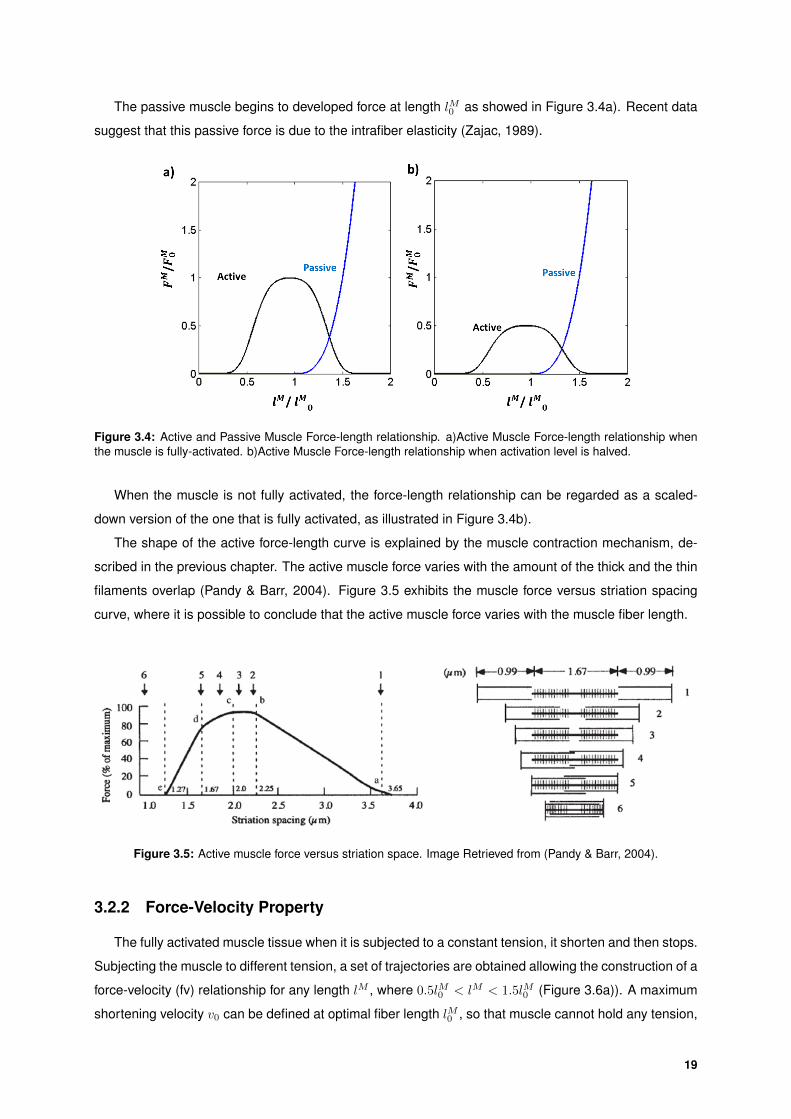
The passive muscle begins to developed force at length lM0 as showed in Figure 3.4a). Recent data
suggest that this passive force is due to the intrafiber elasticity (Zajac, 1989).
Figure 3.4: Active and Passive Muscle Force-length relationship. a)Active Muscle Force-length relationship whenthe muscle is fully-activated. b)Active Muscle Force-length relationship when activation level is halved.
When the muscle is not fully activated, the force-length relationship can be regarded as a scaled-
down version of the one that is fully activated, as illustrated in Figure 3.4b).
The shape of the active force-length curve is explained by the muscle contraction mechanism, de-
scribed in the previous chapter. The active muscle force varies with the amount of the thick and the thin
filaments overlap (Pandy & Barr, 2004). Figure 3.5 exhibits the muscle force versus striation spacing
curve, where it is possible to conclude that the active muscle force varies with the muscle fiber length.
Figure 3.5: Active muscle force versus striation space. Image Retrieved from (Pandy & Barr, 2004).
3.2.2 Force-Velocity Property
The fully activated muscle tissue when it is subjected to a constant tension, it shorten and then stops.
Subjecting the muscle to different tension, a set of trajectories are obtained allowing the construction of a
force-velocity (fv) relationship for any length lM , where 0.5lM0 < lM < 1.5lM0 (Figure 3.6a)). A maximum
shortening velocity v0 can be defined at optimal fiber length lM0 , so that muscle cannot hold any tension,
19

even if fully activated (Zajac, 1989).
When the muscle is not fully activated, the force-velocity relationship can also be regarded to be a
scaled-down version of the one that is fully activated, as it is depicted in Figure 3.6b).
Figure 3.6: .
Force-velocity relationship curve for muscle. a) Force-Velocity relationship curve when the muscle is
fully-activated. b)Force-Velocity relationship curve when activation level is halved.
3.2.3 Elastic Properties of Tendon
When a tensile force is applied to a tendon at its resting length (tendon slack length), the tissue
stretches (Pandy & Barr, 2004). The amount of stretched tendon is called tendon strain and is defined
by Equation 3.5.
εT =∆lT
lTs=lT − lTslTs
(3.5)
Where lTs is the length at which tendon starts to produce force and is called tendon slack length.
The normalization of tendon slack length lTs by optimal fiber length lM0 is denoted by lTs and defines
the compliance of the tendon, once the tendon elasticity is proportional to lTs (Zajac, 1989). Thus the
tendon is considered compliant when lTs is higher than 1, and stiff if otherwise.
The tendon’s stiff (lTs ≤ 1) will be treated as inextensible which implies that its length does not change
over time, i.e., it is always equal to the slack length, and as so the tendon velocity is zero.
On the other hand, a compliant tendon will be described by a force-strain curve (Figure 3.7). This
curve presents three characteristic regions: the toe region, the linear region and the failure region.
The toe region is the initial part of the force-strain curve and describes the nonlinear behaviour of the
material. It is caused mainly by the straightening of the collagen fiber (Spyron & Aravas, 2011) that will
cause the modulus of elasticity (slope of the curve) to increase with strain (Zajac, 1989). The linear
region describes the elastic behavior of the tissue, and the constant slope of the curve defines the
modulus of elasticity of the tendon. The failure region describes plastic changes experience by the
20

tissue, where, initially, a few fibrils start to rupture,and lastly the whole tissue fails (Pandy & Barr, 2004).
Figure 3.7: Force-Strain Tendon Curve (Zajac, 1989).
3.2.4 Modelling of the Musculotendon unit
The musculotendon model was implemented as seen in Figure 3.8. In order to make the model
independent of the muscle activation and force levels the muscle units is considered to be fully activated
(a(t)=1), and the total force produced by the musculotendon unit (FMT ) normalized by the maximum
isometric force (FM0 ) of the muscle. These considerations are represented by the subscript ’a’, and the
tilde sign, which means that (FMTa ) represents the normalized musculotendon force for a fully activated
state of the muscle.
The peak isometric active force (FM0 ), the optimal muscle fiber length (lM0 ), the optimal fiber penna-
tion angle (α0), the maximum shortening velocity (v0) and the tendon slack length (lTs ) are characteristic
parameters of each musculotendon unit and their values were obtained from Delp (Delp et al, 1990).
As represented in Equation 3.6 the contraction dynamics of the musculotendon is characterized by
a first order differential equation (Martin and Schovanec). The derivative of the musculotendon force will
be the model result that allows the determination of the force for the next time step through its numerical
integration. Hence:∂FMT
a
∂t= Kt(
vMT
v0− vM
v0 cos(α)) (3.6)
Where KT is the tendon stiffness calculated according to Zajac (Zajac, 1989) as KT = 30lTs
, vMT and vM
are the musculotendon and muscle velocity respectively and α is the pennation angle.
The musculotendon length (lMT ), velocity (vMT ) and force (FMTa = FTa ) are the model’s input vari-
ables. In the initial time step, an approximation of the musculotendon force must be considered. In order
to guarantee a minimum error for the next instants, this force was calculated through the muscle model
implemented by Pereira (Pereira,2009) , where the tendon length is regarded constant and equal to the
slack length.
The musculotendon length (lMT ) is the distance between the origin and insertion points of the muscle
(DeWoody et al, 1998) and it is determined by the sum of the lengths of the line segments that define
21

the muscle path (Delp & Loan, 1995). The musculotendon velocity (vMT ) is determined by the sum of
the velocities of the line segments along the muscle (Salinas-Aliva, 2009).
Figure 3.8: Musculotendon Model.
22
Looking to Equation 3.6, the derivative of the musculotendon force depends on tendon stiffness and
tendon velocity, which is represent by Equation 3.7.
vT = vMT − vM
cos(α)(3.7)
Once the muculotendon force is already known, the muscle velocity vM and the pennation angle α
must be determined to calculate the tendon velocity. The steps described below and represented in
Figure 3.8 must be taken into account.
1st Step - Determination of tendon length
To determine the tendon length, its compliance characteristic must be taking into account. If the
tendon is stiff, the tendon length is always equal to the slack length. Otherwise, the tendon length will
be determined by the inverse of the force-strain tendon curve relation (Figure 3.7) (Zajac, 1989) that is
represented as follow (Martin & Schovanec):
lT (FTa ) =
lTs (1 +
ln(FTa
0.10377 +1)
91 , 0 ≤ FTa ≤ 0.3086
lTs (1 +FT
a +0.2602937.526 ), 0.3086 ≤ FTa
(3.8)
2st Step - Determination of muscle length
Before determining the muscle length, the pennation angle must be calculated. Since the muscle
thickness (lw) is considered constant, this angle can be determined as:
lw = lM0 sin(α0) = lM sin(α)⇔ α = sin−1(lM0 sin(α0)
lM) (3.9)
Using Equations 3.2 and 3.9, the expression that allows the calculation of the angle between the
muscle fibers and the tendon is obtained:
α = tan−1(lM0 sin(α0)
lMT − lT) (3.10)
The muscle length can now be calculated solving the Equation 3.2 as shown in Figure 3.3.
3st Step - Determination of Passive Muscle Force and of the Force-length relationship
The passive force and active force (fl(lM )) are governed by Equations 3.11 and 3.12 respectively
(Silva, 2003).
FPE(lM ) =
0, lM0 > lM (t)
8FM
0
(lM0 )3(lM − lM0 )3, 1.63lM0 ≥ lM (t) ≥ lM0
2FM0 , lM (t) > 1.63lM0
(3.11)
23

fl(lM ) = FM0 exp
−[[ 94 (lM (t)
lM0
− 1920 )]4− 1
4 [− 94 (
lM (t)
lM0
− 1920 )]2]
(3.12)
4st Step - Determination of the Force-velocity relationship
Through the Hill-type model equations, an expression for the muscle velocity is obtained. Considering
the relation expressed in Equation 3.3 and Equation 3.4, an equation for the calculation of vM is achieved
(Equation 3.13).
vM = v0f−1v (
FTa F
M0
cos(α) − FPE(lM )
fl(lM )) (3.13)
So the force-velocity is given by:
fv(vM ) =
FTa F
M0
cos(α) − FMPE(lM )
fl(lM )=FMCE(lM )
fl(lM )(3.14)
Where FMCE is the maximum available contractile force.
In the cases where a singularity is present, fl(lM )→ 0, the condition fl(lM ) > 0.1FM0 was considered
in order to maintain fv between physiological values (Millard et al, 2013).
5st Step - Determination of the muscle velocity
The inverse of the force-velocity relationship (Anderson, 2007), represented in Figure 3.6a), which
allows the calculation of the muscle velocity according to the force calculated in Equation 3.14, will be
expressed as:
vM = −v0(0.18 log(
fvFM
0
− fvFM
0+ 1.8
) + 0.04) (3.15)
24

4Integration of a Musculotendon Model
in the framework of Multibody
Formulation with Natural Coordinates
Contents
4.1 Introduction of Multibody Dynamics with Natural Coordinates . . . . . . . . . . . . . 26
4.2 Integration of Musculotendon Model within APOLLO . . . . . . . . . . . . . . . . . . 39
25

4.1 Introduction of Multibody Dynamics with Natural Coordinates
The analysis of the movement in this study was carried in the framework of a multibody dynamics
analysis with natural coordinates. An existing Fortran code called APOLLO was adapted in order to
integrate the musculotendon model.
This chapter is divided in two parts. The first one, introduces the multibody dynamics analysis starting
by the basic concepts (e.g. multibody systems, kinematic pairs), the coordinated system used and
kinematic analysis, and ending in dynamics analysis (i.e. forward and inverse dynamic analysis). In
the second part, the way the musculotendon model was implemented is explained for both dynamic
analyses types and a simple validation example of a upper limb elbow’s flexion/extension is presented.
4.1.1 Basic Concepts
Multibody dynamics aims to simulate the behaviour of a multibody system, where its geometric and
dynamic characteristic have been defined. It allows for the visualization of the successive responses of
a multibody system, i.e., the simulation of its behavior and operation over the entire workspace and over
a certain period of time (Jalon and Bayo, 1994).
A multibody system is defined as an assembly of rigid bodies joined together through kinematic
pairs or joints, having the possibility of relative movement between them. A kinematic pair influences
the degrees of freedom to constrain the relative motion. Sometimes, the elements that constitute the
multibody system are not in direct contact but are interrelated through force transmission elements, such
as springs and dampers (Jalon and Bayo, 1994).
Kinematic Analysis is the study of motion of a multibody system regardless of the forces and reactions
that generate it (Jalon and Bayo, 1994). The position, velocity and acceleration of every element of the
system are obtained and analyzed (Silva, 2003) independently of the forces and inertia characteristics
of elements (e.g. mass, moments of inertia and position of the center of gravity) (Jalon and Bayo, 1994).
Since this characteristics are not considered, the motion must be specified in terms of position, velocity
and acceleration of its driving elements, while the motion of the remaining elements are obtained using
the kinematic constraint equations that describe the topology of the system, its kinematic pairs and rigid
body properties (Silva, 2003).
Dynamics Analysis involves knowledge of the forces that act on the multibody system and also its
inertial characteristics. It is performed after the kinematic analysis and can be of two different types,
forward and inverse dynamics analysis (Jalon and Bayo, 1994). The first one consists in obtaining the
movement of a multibody system resulting from the application of external forces. The second one aims
to determine the internal and external forces developed in/by the multibody system, considering the
movement observed, the topology of the system and the kinematic constraints (Silva, 2003).
26

4.1.2 System of Coordinates
In kinematic and dynamic analysis of multybody system a set of coordinates must be selected to
define clearly the position, velocity and acceleration of the multibody system at all instants of time.
A multibody system can be described with different types of coordinates: independent and dependent
coordinates. The number of independent coordinates match with the number of degrees of freedom of
the multibody system. On the other hand, in a system defined with dependent coordinates, their number
is greater than the system’s degrees of freedom.
Dependent coordinates were used to determine the position and orientation of each body. They are
interrelated through constraint equations that are normally non-linear and in a number that is the result
of the difference between the number of dependent coordinates and the number of degrees of freedom
(Jalon and Bayo, 1994).
In this work, natural coordinates are used to define the multibody system. In three-dimensional
multibody systems, each body is defined at least with two points and two unit vectors and the position
and angular orientation of each body is defined by the cartesian coordinates of these points and of unit
vectors, respectively. With this way of defining rigid bodies, the Euler parameters or Euler or Bryant
angles are not required simplifying this way the problem to solve (Jalon and Bayo, 1994).
There are a lot of possible combinations between points and unit vectors, and the motion of the ele-
ment will be characterized through the movement of both (Jalon and Bayo, 1994). With this formulation,
it is possible that two adjacent rigid bodies share points and vectors (Silva, 2003), which means that a
point can be located between two linked elements (e.g.,on the joints) and a unit vector can be positioned
on the joints defining the direction of the rotational or translational axis (Jalon and Bayo, 1994). This
features allows for the reduction of the number of coordinates necessary to characterize the system and
the consequently of the number of algebraic constraint equations (Silva, 2003). On the other hand, the
constraint equations used to defined rigid bodies and joint conditions are quadratic or linear, implying
that their contribution to the Jacobian matrix to be linear or constant. Design variables, like lengths
and angles, appear explicitly, allowing parametric and variational design, kinematic synthesis, sensitivity
analysis and optimization which is a benefit from the use of these coordinates (Jalon and Bayo, 1994).
4.1.3 Kinematics
The Cartesian coordinates of every point and vector used to define a generic mechanical system
in a kinematic or dynamic analysis are pooled in the column vector q. This vector is called vector of
generalized coordinates, since is constituted by the set of coordinates that define the configuration of
the system at any time (Silva, 2003). For a system defined with n points and m vectors, the vector of
generalized coordinates is characterize as follows.
q = {xP1 yP1 zP1 ... xPn yPn zPn xV1 yV1 zV1 ... xVm yVm zVm}T (4.1)
27

Where x,y and z are the coordinates of the points and vectors, and the P and V represent the points and
the unit vectors respectively. This vector is comprised of three times the sum of the number of point and
the number of unit vectors (i.e., nc=3(m+n)).
In a multibody formulation with natural coordinates, kinematic constrains equations, which are as-
semble in the column vector Φ, must be defined. These constraints can be divided in scleronomic
constraints that are normally used to define rigid bodies and to describe kinematic pairs and, rheonomic
constraints that are associated with driver actuators (Silva, 2003). Hence, vector Φ(q, t) is organized as:
Φ(q, t) = {Φ1(q) ... Φns(q) Φns+1(q, t) ... Φns+nr(q, t)}T = 0 (4.2)
Where Φi represent the ith kinematic constraint equation, ns the total number of scleronomic constraints,
nr the total number of rheonomic constraints and 0 is the vector null (Silva,2003). The first constraints
(scleronomic constraints) do not depend explicitly on time, instead of what happens with the second
ones (rheonomic constraints). The total number of constraints, called holonomic constraints, result from
the sum of both type of constraints (i.e., nh=ns+nr ).
In the construction of this vector different types of constraints are considerer in this work: rigid body
constraints to model constant length between points that belong to the same body, joint constraints to
define the relative motion between elements and driver constraints to prescribe the motion of the system.
4.1.3.A Kinematic Analysis
The kinematic analysis, as reported earlier, consists in determine the positions, velocities and ac-
celerations of each rigid body, taking into account the driver information and the initial position of the
system. At each instant of time, a set of positions that satisfy the kinematic constraint equations are
obtained. This set of positions are called kinematic consistent positions and are determined solving
Equation 4.2 in order to the vector of generalize coordinates q.
Equation 4.2 is composed by a group of nonlinear equations that is solved using the Newton-Raphson
method. This iterative method has quadratic convergence in the neighborhood of the solution, which is
achieved by the linearization of the system presented in Equation 4.2. This linearization consists in
substitute the system of equation with the first two terms of its expansion in a Taylor series around a
certain approximation qi to the desired solution (Jalon and Bayo, 1994). Therefore, for each instant of
time, the system become as follows.
Φ(q, t) ∼= Φ(qi) + Φq(qi)(q− qi) = 0 (4.3)
where Φq(qi) is the Jacobian matrix of the constraint equations, evaluated at qi, i.e., the matrix of the
28

partial derivatives of these equations in order to the generalized coordinates (Jalon and Bayo, 1994):
Φq =
∂φ1
∂q1
∂φ1
∂q2... ∂φ1
∂qn
∂φ2
∂q1
∂φ2
∂q2... ∂φ2
∂qn
... ... ... ...
∂φm
∂q1
∂φm
∂q2... ∂φm
∂qn
(4.4)
Since the Newton-Raphson method is an iterative procedure, the approximate result, obtain from
Equation 4.3, for the next iteration is obtained defining q = qi+1. Representing 4qi = qi+1 − qi as the
residual for the actual iteration (Silva, 2003) Equation 4.3, becomes:
Φq4qi = −Φ(qi) (4.5)
In the presence of redundant constraint equations the Jacobian matrix is no longer a square matrix
and the least-square formulation is used (Jalon and Bayo, 1994):
(ΦTq Φq)i4qi = (ΦT
q )i(Φq)i (4.6)
This algorithm converges to the exact solution of all constraint equations (Jalon and Bayo, 1994).
The velocity equations are obtain by differentiating the Equation 4.2 in order to time. The result
obtained is:
Φ(q, q, t) =dΦ(q, t)
dt=∂Φ(q, t)
∂t+∂Φ(q, t)
∂q
dq
dt= 0 (4.7)
Where ∂Φ(q,t)∂t are the partial derivatives of the constraints in order to time and can be represent by
ν, ∂Φ(q,t)∂q is the Jacobian matrix and dq
dt are the derivatives of the generalize coordinates in order to
time, that can be represent as q. This vector contains the velocities of the points and unit vectors of the
multibody system. Equation 4.7, updated with this definitions, becomes as follows:
Φqq = ν (4.8)
The acceleration vector is obtain differentiating the velocity vector in order to time (Equation 4.9).
Φ(q, q, q, t) =dΦ(q, q, t)
dt= Φqq + (Φqq)qq + νt = 0 (4.9)
Where vector νt is the partial derivatives of the vector ν in order to time. Defining vector γ as:
γ(q, q, t) = νt − (Φqq)qq, (4.10)
then the generalized accelerations of the system can be calculated as:
Φqq = γ (4.11)
29

Equations 4.8 and 4.11 represent system of linear equations with the same leading matrix Φq. The
process applied in Equation 4.6 is also applied in the velocity and acceleration analysis in face of redun-
dant constraints (Silva, 2003).
4.1.4 Dynamics
In this subsection the equations used in a multibody dynamic analysis with natural coordinates are
presented.
4.1.4.A Equations of Motion
In a dynamic problem defined with dependent natural coordinates the motion of the entire multibody
system is determined establishing the dynamic equilibrium condition through a system of second order
differential equations called equations of motion.
Equations of motion can be formulated through several methods, like the application of Lagrange’s
equation and the principle of virtual power (Jalon and Bayo, 1994).
The principle of virtual power is the method used is this work. This principle establishes that the sum
of the virtual power produced by the inertial and external forces that act in a mechanical system is zero
at any instant of time (Silva, 2003). This is represented by Equation 4.12.
q∗T (Mq− g) = 0 (4.12)
Where q∗ is the virtual velocity vector that belongs to the null space of the Jacobian matrix. Mq de-
scribes the inertial forces, where M is the global mass matrix and q the vector of generalized accelera-
tions. Vector g is called the generalized force vector and contains the externally applied forces and the
velocity-dependent inertial forces.
The internal forces, which are related with the kinematic constraints, produce no virtual power, and
therefore are not included in Equation 4.12. However, through the Lagrange multipliers method the
virtual power of these forces can be calculated an included in Equation 4.12. This method defines the
generalized force vector that contains the internal forces gΦ as presented in Equation 4.13.
gΦ = ΦqTλ (4.13)
Where λ is the Lagrange multipliers vector that represents the magnitude of the internal forces and Φq
is the Jacobian matrix whose rows represent their direction. Considering the properties of the virtual
velocity vector, the product q∗TΦqTλ belongs to the null space of the Jacobian matrix (Silva, 2003):
q∗T (Mq− g + ΦqTλ) = 0 (4.14)
The equations of motion (EOM) that describe the constrained multibody system are represented by
30

the equation presented between the brackets:
Mq− g + ΦqTλ = 0 (4.15)
4.1.4.B Muscle Forces
The muscle structure in this work is defined by the cartesian coordinates of a set of points (i.e.,
origin (o), insertion (i) and via-points(vp), interconnected by line segments. Via-points allow for a better
definition of the muscle geometry bringing it closer to the real one (Silva, 2003). Although the aim is
to describe the muscle the more closer to reality as possible, some simplifying assumptions need to
be considered. Those are the straight line segments, constant cross-sectional area no wrap around
structures in its via-points.
Considering therefore a muscle force FM with a magnitude FM , a number of forces (nf ) is applied to
the set of points that define the muscle. This number is given by 2vp + 2, which means that if the muscle
is not defined with any via-point, the forces are only two and are applied in the origin and insertion sites
of the muscle respectively.
A muscle with via-points is defined by a set of unit vectors that are used to define the orientation of the
muscle forces in each muscle segment (u1,u2, ...,ud), where d is calculated as d = vp+1 (Pereira,2009).
Hence, the muscle force, applied with a magnitude FM to a point p with direction ud is represent as:
FMp = udFM (4.16)
In the formulation used in this work, muscles are defined as forces that represent the action of the
muscle structure. The magnitude of the force exerted by a muscle will be the same for different length
locations and will correspond to the force exerted by the whole muscle FM (Pereira,2009).
Generalized Muscle forces
Muscle forces need to be converted into generalized forces in order to be included in the multibody
system. These forces will be considered as external forces and are processed in this work as described
by Jalon and Bayo (Jalon and Bayo, 1994) and Silva (Silva, 2003). Observing Figure 4.1, a rigid body
(e) with a local reference frame oξηζ was defined by two points i and j and two non-planar vectors u and
v whose cartesian coordinates are described in an inertial reference frame oxyz.
31

Figure 4.1: Basic Rigid Body (e) (Pereira,2009).
In this rigid body a generic force FM is applied in point p. The global coordinates rp of this point are
related to the cartesian coordinates of ri , rj , u and v as follows.
rp − ri = c1(rj − ri) + c2u + c3v (4.17)
The coefficients c1, c2 and c3 scale the coordinates of vector rip in the reference frame formed by
vectors rij , u and v. Resolving in order to rp Equation 4.18 is obtained .
rp = [(1− c1)I3 c1I3 c2I3 c3I3]3×12
ri
rj
u
u
12×1
= Cpqe (4.18)
Matrix Cp express the Cartesian coordinates of any given point p that belong to the rigid body e
as a linear combination of generalised coordinates qe used to describe that element. This matrix is
constant during the entire analysis, once it depends exclusively of local vectors. The matrix Cq must be
assembled at any point where a force is applied. The ci coefficients are calculated by adapting Equation
4.18 to the local frame (Equation 4.19). Hence:
(r′p − r′i ) = [r′ij u′ v′]
c1
c2
c3
= X′c (4.19)
Where X′
= [r′ij u′ v′]. This matrix present always an inverse and therefore the Equation 4.19 can
be resolved in order to c, yielding:
c = X′−1(r′p − r′i) (4.20)
32

The generic muscle FMp can now be expressed in terms of gFM
pe , an equivalent term expressed in
term of the generalized coordinates of the rigid body (Pereira,2009). Knowing that the virtual work done
by concentrated forces and their generalized term is the same, them:
δW = δrTp FMp = δqTe gFM
p
e = δqTe CTp FMp (4.21)
from which the mathematical expression that describes FMp in terms of gFM
pe is obtained:.
gFM
pe = CT
p FMp = CTp ud′FM (4.22)
To represent the muscle forces for the entire system, global vector gFMp of size nc is created from the
manipulation of the generalized element vector gFM
pe by means of a simple assembled process (Silva,
2003).
This vector can be represent as illustrated in Equation 4.23, taking into account the number of rigid
bodies nb present in the entire system and the respective number of via points that define the muscle in
each one.
gFMp =
nb∑i=1
gFM
pe(i) =
nb∑i=1
vp+2∑j=1
gFM
pe (4.23)
Since FMp can be represent by the Hill-type muscle model components, according to Equation 3.3
then, the following equation is obtained,
gFM = gFM
CE + gFM
PE (4.24)
Where gFM
CE and gFM
PE represent the generalized force vectors for the contractile and passive elements
respectively.
According to the relation between the muscle force and the musculotendon force present in Equation
3.4, Equation 4.25 is also obtained.
gFMT = (gFM
CE + gFM
PE) cos(α) (4.25)
Which, by its turn, can be expressed in terms of the muscle activation aM (Equation 4.26), yielding:
gFMT = (gFM
CEaM + gFM
PE) cos(α) (4.26)
Where gFM
CE is the generalize force vector of the maximum contractile force of a muscle in a given state.
4.1.4.C Inverse Dynamic Analysis
The Inverse Dynamic (ID) Analysis aims to determine the internal and external forces developed in/by
the multibody system, considering the movement observed, the topology and the kinematic constraints.
This kind of analysis allows the calculation and evaluation of reaction forces and moments in the joints
33
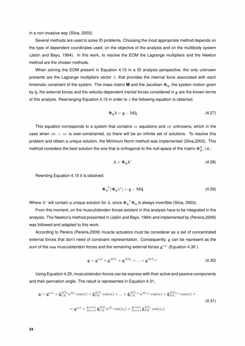
in a non-invasive way (Silva, 2003).
Several methods are used to solve ID problems. Choosing the most appropriate method depends on
the type of dependent coordinates used, on the objective of the analysis and on the multibody system
(Jalon and Bayo, 1994). In this work, to resolve the EOM the Lagrange multipliers and the Newton
method are the chosen methods.
When solving the EOM present in Equation 4.15 in a ID analysis perspective, the only unknown
presents are the Lagrange multipliers vector λ, that provides the internal force associated with each
kinematic constraint of the system. The mass matrix M and the Jacobian Φq, the system motion given
by q, the external forces and the velocity-dependent inertial forces considered in g are the known terms
of this analysis. Rearranging Equation 4.15 in order to λ the following equation is obtained.
Φqλ = g −Mq (4.27)
This equation corresponds to a system that contains nc equations and nh unknowns, which in the
case when nh > nc is over-constrained, so there will be an infinite set of solutions. To resolve this
problem and obtain a unique solution, the Minimum Norm method was implemented (Silva,2003). This
method considers the best solution the one that is orthogonal to the null-space of the matrix ΦTq , i.e.:
λ = Φqλ∗ (4.28)
Rewriting Equation 4.15 it is obtained:
ΦqT (Φqλ
∗) = g −Mq (4.29)
Where λ∗ will contain a unique solution for λ, since ΦqTΦq is always invertible (Silva, 2003).
From this moment, on the musculotendon forces existent in this analysis have to be integrated in the
analysis. The Newton’s method presented in (Jalon and Bayo, 1994) and implemented by (Pereira,2009)
was followed and adapted to this work.
According to Pereira (Pereira,2009) muscle actuators must be considerer as a set of concentrated
external forces that don’t need of constraint representation. Consequently, g can be represent as the
sum of the nm musculotendon forces and the remaining external forces gext (Equation 4.30 ).
g = gext + gMT1 + gMT2 + ...+ gMTnm (4.30)
Using Equation 4.25, musculotendon forces can be express with their active and passive components
and their pennation angle. The result is represented in Equation 4.31.
g = gext + gMT1
CE aM1 cos(α) + gMT1
PE cos(α) + ...+ gMTnm
CE aMnm cos(α) + gMTnm
PE cos(α) =
= gext +∑nmi=1 gMTi
CE aMi cos(αi) +∑nmi=1 gMTi
PE cos(αi)
(4.31)
34

Replacing Equation 4.31 in Equation 4.27 it is obtained:
ΦqTλ = gext +
nm∑i=1
gMTi
CE aMi cos(αi) +
nm∑i=1
gMTi
PE cos(αi)−Mq (4.32)
Which can be rewrited in a more compact form:
[ΦT
q −χT]λa
= gext + gMTPE cos(α)−Mq (4.33)
Where χ is a matrix that contains all the generalized maximum available contractile force vectors of all
the muscle of the system (Equation 4.34), and a is the vector of the corresponding muscle activations
(Equation 4.35).
χ =
gMT1
CE cos(α1)
...
gMTnm
CE cos(αnm)
(4.34)
a =
aM1
...
aMnm
(4.35)
When the musculotendon forces are included in the EOM, the system will contain infinite solutions
since it has nc equation and nh+nm unknowns. This can be physiologically associated with muscle
redundancy, which means that a infinite number of muscle combinations may result to represent a de-
termined motion. To solve this problem, optimization techniques, as described hereafter, are used to
found the solution that best fulfils a given physiological criterion.
4.1.4.D Optimization
For a specific movement there will be an infinite set of muscle force combinations to produced it.
The CNS is responsible to solve this redundant problem of the musculoskeletal system by choosing the
optimal activation combinations to execute that specific movement.
In the Newton method used before to deal with the muscles forces a redundant system also exists.
To solve this indeterminate problem, optimization techniques are used to find the optimal solution, re-
garding a set of optimization constraints, that minimizes a given cost function. The cost function is a
mathematical expressions that simulates the way that the CNS recruite the muscles for a given move-
ment.
For the purpose of calculating the redundant muscle forces, the optimization process aims to find the
solution of the equation,
An×mxm×1 = bn×1 (4.36)
Where x is the unknown and A is a rectangular matrix with n > m, that minimizes a given cost function.
In every optimization problems, an initial guessed solution x0 must be given to the system. In this ID
35

formulation the column vector x (Equation 4.37) is composed by λ and a since these are the unknowns
of the problem.
x = λ =
λa (4.37)
The solution of the stated optimization problem is subjected to a set of optimization constraints that
in the present case are the EOM of the multibody system. The constraints derived from the equation
of motion are the equality constraints feq (Equation 4.38) in which its gradient will be needed for the
optimization routines (Equation 4.39).
feq =
f1
...
fnc
=[ΦT
q −χT]λa
+ Mq− (gext + gMTPE cos(α)) = 0 (4.38)
∇feq
λ
a
=
[ΦT
q −χT]
(4.39)
The Lagrange multiplier attributed to each kinematic driver holds the force contribution that is neces-
sary to be provided by that driver for the execution of the prescribed movement, when muscles are not
included. Considering λ∗R as the Lagrange multipliers associated with the drivers of the joints crossed by
muscles in the redundant problem, then when muscles are studied the contribution of these joint drivers
in the system needs to be eliminated and shifted to the corresponding muscle activation. Theoretically
this will be possible if this Lagrange multipliers are set to zero, but in practical terms these are in fact
maintained between ε, where ε is a user specified value (Equation 4.41).
|λ∗R| ≤ ε (4.40)
Accordingly, the values of muscle activations a are kept within these physiological limits, i.e., always
positive and limited between 0 and 1.
0 ≤ aM ≤ 1, for m = 1, ..., nm (4.41)
The others Lagrange multipliers λR and λS , that are related to the rheonomic and scleronomic
constraints, respectively, have no limitations, i.e.,
−∞ ≤ λR ≤ +∞ (4.42)
−∞ ≤ λS ≤ +∞ (4.43)
Concluding, the optimization process implemented by Pereira (Pereira,2009) in APOLLO is ex-
36

pressed in Equation 4.44.
Given : x = λ =
λa
Minimise : F(x) =∑nmi=1(σMi
CE)3
Subject to :
feq = 0
−∞ ≤ λR ≤ +∞
−∞ ≤ λS ≤ +∞
|λ∗R| ≤ ε
0 ≤ aM ≤ 1
(4.44)
Where σM =FM
CM
A0is the muscle stress that are used in the cost function that consists in the sum of the
cube of each muscle contractile tension.
In this work the DOT 5.0 - Design Optimization Tools, was used as optimizer (Vanderplaats, 1999).
This package is a well-known optimization program that contain the MFD, the SLP and the SQP opti-
mization method to solve the constrained NLP problem (Silva,2003)
4.1.4.E Forward Dynamic Analysis
Forward dynamic (FD) analysis allows the calculation of a dynamic response of a constrained multi-
body system owing to the effect of external applied forces (Silva, 2003), that in this case are the mus-
culotendon forces. The aim of this analysis in to calculate the system’s motion and the internal forces
developed.
In this work, the implementation of the FD methodology takes into account the vector of muscle
activations aM , that is obtained from inverse dynamics after the optimization procedure. So the gen-
eralized forces vector g is known and the vector q has to be determined. Equation 4.15 becomes an
indeterminate system of nc second order ordinary differential equations (ODE) with nc+nh unknowns.
To solve this indetermination nh equations must be added (described in Section 4.1.3.A), resulting in the
following matrix system. M ΦTq
Φq 0
q
λ
=
g
γ
(4.45)
Once this system is solved, the generalized coordinates of the system q can be obtain through
numerical integration of the acceleration’s vector in order to time. The initial state of the system, the
initial position q0 and velocity q0 must therefore be given, making sure that there are according with the
kinematic constraints of the system, which is guarantied when Equations 4.46 and 4.47 are performed
for the initial value of the problem.
Φ(q0) = 0 (4.46)
Φqq0 = ν(t0) (4.47)
37

In the flowchart present in Figure 4.2 the FD analysis process is represented.
Figure 4.2: Direct Integration Algorithm (Silva,2003).
First the consistency of the initial conditions must be verify. Then an iterative method called Aug-
mented Lagrange Formulation (ALF) that consists of a penalty-type formulation that aims to stabilize
the EOM is used to solve the EOM (Silva, 2003). The Lagrange multipliers can be calculated when
required, which implies that if they are removed from Equation 4.45 it becomes a second order ODE
with nc equations where only the vector q is determined.
After obtained the acceleration’s vector, this is integrated in order to time in order to obtain the
generalized coordinates of the system. The generalized velocities and accelerations vectors (q and q)
are assembled in a vector yt (Pereira,2009).
yt =
q
q
(4.48)
Integrating in time this vector using a direct integration method, a vector containing the generalized
positions and velocities for the next time step is obtained (Equation 4.49).
yt+∆t =
q
q
(4.49)
With this, the positions, velocities and time of the system are update for the next cycle where the con-
sistency of the new values of the system don’t need to be checked as yt+∆t is obtained in a consistent
form.
38

4.2 Integration of Musculotendon Model within APOLLO
The integration of Musculotendon Model in program APOLLO in an inverse and forward dynamics
perspective will be described in the following subsections. It is important to note that the musculotendon
model will be the same in both analysis. These two type of analysis, as well as the model were explained
before in order to better understand this integration.
In both analysis, a simple application example of elbow extension/flexion is presented, where only
one musculotendon actuator was used, to analyse the results obtained by the model.
4.2.1 Inverse Dynamic Analysis
In the flowchart present in Figure 4.3 it is possible to observe the integration of the musculotendon
model in an inverse dynamic analysis.
Figure 4.3: Flowchart of inverse-dynamics analysis with the Musculotendon Model integrated .
As mentioned before this type of analysis aims to determine the internal and external forces devel-
oped in/by the multibody system. The solution of this problem requires an optimization technique to
solve the EOM in order to the unknowns, the Lagrange multipliers and the muscle activations.
For each time step the vector that contains the position, velocity and acceleration of each segment
are known. Otherwise, the fully activated musculotendon force is determined through numerical inte-
gration ensuring this value always for the next time step. This force will be essential, together with the
musculotendon length and velocity, to obtain the maximum contractile force, the passive force and the
pennation angle through the musculotendon model. These values will integrate the EOM.
After the muscle activation is determined, the musculotendon and muscle force of the current time
step is obtained as shown in the ’Update Forces’ section (Figure 4.3).
39
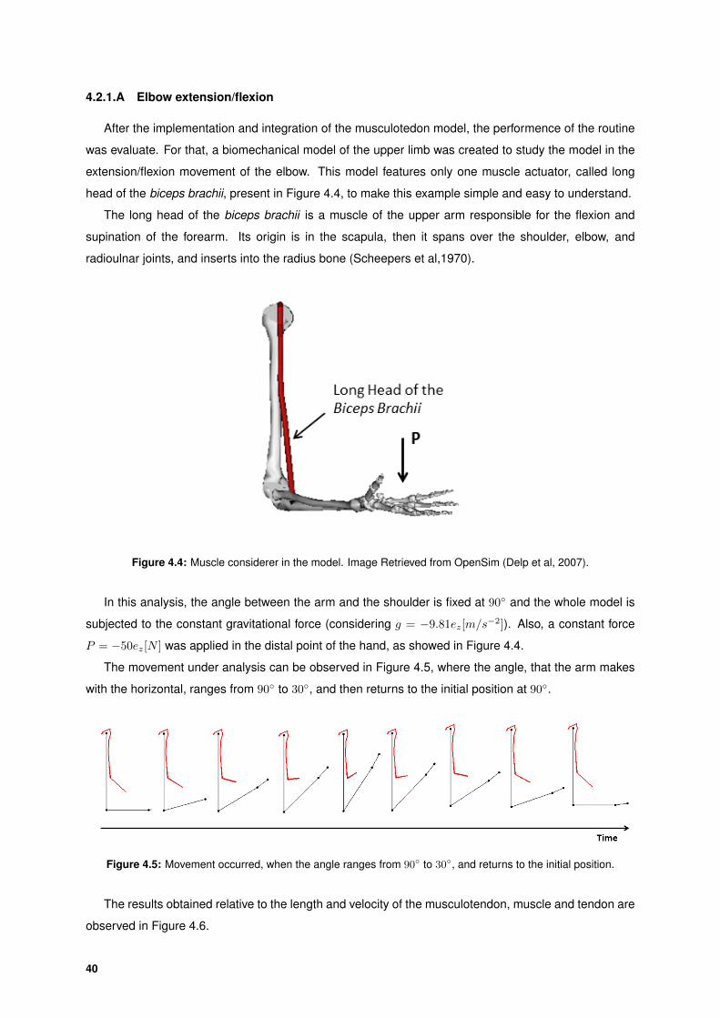
4.2.1.A Elbow extension/flexion
After the implementation and integration of the musculotedon model, the performence of the routine
was evaluate. For that, a biomechanical model of the upper limb was created to study the model in the
extension/flexion movement of the elbow. This model features only one muscle actuator, called long
head of the biceps brachii, present in Figure 4.4, to make this example simple and easy to understand.
The long head of the biceps brachii is a muscle of the upper arm responsible for the flexion and
supination of the forearm. Its origin is in the scapula, then it spans over the shoulder, elbow, and
radioulnar joints, and inserts into the radius bone (Scheepers et al,1970).
Figure 4.4: Muscle considerer in the model. Image Retrieved from OpenSim (Delp et al, 2007).
In this analysis, the angle between the arm and the shoulder is fixed at 90◦ and the whole model is
subjected to the constant gravitational force (considering g = −9.81ez[m/s−2]). Also, a constant force
P = −50ez[N ] was applied in the distal point of the hand, as showed in Figure 4.4.
The movement under analysis can be observed in Figure 4.5, where the angle, that the arm makes
with the horizontal, ranges from 90◦ to 30◦, and then returns to the initial position at 90◦.
Figure 4.5: Movement occurred, when the angle ranges from 90◦ to 30◦, and returns to the initial position.
The results obtained relative to the length and velocity of the musculotendon, muscle and tendon are
observed in Figure 4.6.
40
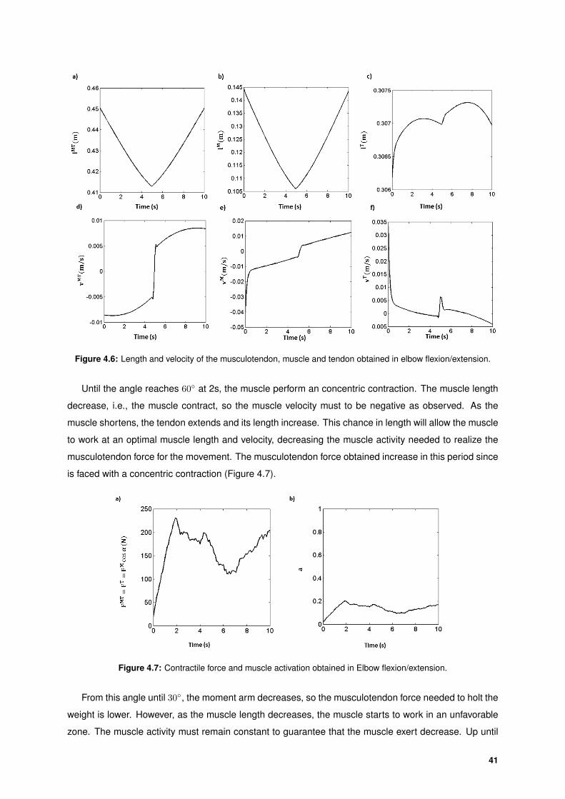
Figure 4.6: Length and velocity of the musculotendon, muscle and tendon obtained in elbow flexion/extension.
Until the angle reaches 60◦ at 2s, the muscle perform an concentric contraction. The muscle length
decrease, i.e., the muscle contract, so the muscle velocity must to be negative as observed. As the
muscle shortens, the tendon extends and its length increase. This chance in length will allow the muscle
to work at an optimal muscle length and velocity, decreasing the muscle activity needed to realize the
musculotendon force for the movement. The musculotendon force obtained increase in this period since
is faced with a concentric contraction (Figure 4.7).
Figure 4.7: Contractile force and muscle activation obtained in Elbow flexion/extension.
From this angle until 30◦, the moment arm decreases, so the musculotendon force needed to holt the
weight is lower. However, as the muscle length decreases, the muscle starts to work in an unfavorable
zone. The muscle activity must remain constant to guarantee that the muscle exert decrease. Up until
41

the lower arm reaches 60◦, the musculotendon force decrease.
From 60◦ until the starting position, the moment arm increases which leads to an increase of the
musculotendon force. The muscle length increases, and the muscle velocity is positive. As the muscle
lengthens, the tendon shortens and its length decreases.
4.2.2 Forward Dynamic Analysis
The flowchart presented in Figure 4.8 shows how the musculotendon model was integrated in the
forward dynamic analysis.
Figure 4.8: Flowchart of forward-dynamics analysis with the Musculotendon Model integrated.
Unlike what happens with the previous analysis, a forward analysis aims to obtain the movement
of a multibody system resulting from the application of external forces. From the beginning the muscle
activations are known and the positions, velocities and accelerations vectors must be determined.
Through musculotendon model also the maximum contractile force, the passive force and the pen-
nation angle are determined. These variables together with the muscle activation allow the calculation
of the musculotendon forces that will be integrated in the EOM. As mentioned before, through EOM the
Lagrange multipliers and the acceleration vectors are obtained.
As the muculotendon force is controlled by a differential equation, the value of the fully activated
musculotendon force derivative is assembled to the vector y to be integrated with the velocities and
acceleration variables. This result in a vector y that contains the positions, velocities and fully activated
musculotendon forces for the next time step.
42

4.2.2.A Elbow extension/flexion
The same biomechanical model was used in the forward dynamic analysis. The muscle activation
obtained in the previous analysis (Figure 4.7) are used in this analysis to obtain the musculotendon
forces, as well as, the length and velocity, like the example before.
The results obtained are presented in Figure 4.9 and Figure 4.10. As expected, the movement
observed is the same as well as the musculotendon force, length and velocity of the musculotendon,
muscle and tendon units.
Figure 4.9: Length and velocity of the musculotendon, muscle and tendon obtained in shoulder flexion/extension.
Figure 4.10: a)Contractile force and b) muscle activation obtained in elbow flexion/extension.
43

44

5Biomechanical Model
Contents
5.1 Model Description . . . . . . . . . . . . . . . . . . . . . . . . . . . . . . . . . . . . . . . 46
5.2 Implementation Model . . . . . . . . . . . . . . . . . . . . . . . . . . . . . . . . . . . . 49
5.3 Anthropometric Data . . . . . . . . . . . . . . . . . . . . . . . . . . . . . . . . . . . . . 50
5.4 Musculotendon Apparatus . . . . . . . . . . . . . . . . . . . . . . . . . . . . . . . . . . 52
45

Over the past thirty years, the development of dependable mathematical models of the human body
for the biomechanics community has been of greater interest to simulate and analyze the mechanical
behaviour of the human body in their day to day activities. This sort of simulation is very important in a
set of applications like, athletic sports, to improve the performance and to optimize the design equipment;
ergonomic studies, to evaluate conditions for comfort and efficiency of the interaction between the human
body and the environment; and orthopedics, to create and analyze prosthesis.
This mathematical models of the human body, also called biomechanical models, describes the hu-
man body in terms of its anthropometry, physiology and topology, that vary depending on the objectives
of the analysis.
In this work, a whole body response biomechanical model are defined using the multibody formula-
tion described in Chapter 4. In the following chapters, the biomechanical model used will be described
in detail taking into to account its anthropometric data, that include the body size segments, the mass,
inertia and center-of-mass location of the principal anatomical segments, and muscle apparatus. Also,
the way that will be implemented will be outlined.
5.1 Model Description
The main propose of this work is to develop a model that allow the study of the main kinematic and
dynamic patterns during different types of human activities like walking, running and jumping. Due to
its complex kinematic structure, it can be used to simulate human movements in forward and inverse
dynamics analysis.
The defined model divides the whole body in eight segments: the HAT, composed by head, arms and
torso, the pelvis, composed by L4-L5 to greater trochanter (Winter, 2000), thigh, leg and foot (Figure 5.1
a) and c)).
The HAT, adapted by the model implemented by Anderson and Pandy (Anderson & Pandy,2007),
was considerer as a single rigid body as seen in Figure 5.1 c).
46

Figure 5.1: Biomecanical Model. a)Human Skeletal Image Retrieved from OpenSim (Delp et al 2007). b)FootSkeletal. Image Retrieved from OpenSim (Delp et al 2007). c)Biomecanical Model Division
The foot was described using the model implemented by Malaquias (Malaquias, 2013). It is divided in
three segments: the rear-foot, that includes the calcaneus; the mid/fore-foot, that includes the Navicular,
cuboid, the three cuneiform bones and metatarsus; and the toes, that are composed by the phalanges
(Figure 5.1 b) and c) ).
The different segments are connected through a set of 13 joints:
1. Pelvis Joint
2. Hip Joint
3. Knee Joint
4. Talocrural joint
5. Talocalcaneal or subtalar joint
6. Midtarsal or Chopart’s joint
7. Metatarsophalangeal joint
The insertion of the mid/fore foot in the model increase the reliability, allowing the study of the move-
ments that occurs between the midtarsal and tarsometatarsal joint. Also, to decrease the integration
time of the model, the talus was consider as a massless link, which means that the axis of the Talocrural
and the talocalcaneal joint do not intersect and have a constant distance between them (Malaquias,
2013).
This model has therefore 27 degrees-of-freedom (DOF). Once they are associated with the type of
motion that each joint is able to realize. They result from:
• 2 DOF - Flexion/Extension and lateral extension at the Pelvis Joint;
• 2× 2 DOF - Flexion/Extension and Abduction/Adduction at the hip joint;
• 2× 1 DOF - Internal thigh rotation;
• 2× 1 DOF - Flexion/Extension of the Knee Joint;
47

• 2× 1 DOF - Internal leg rotation;
• 2× 1 DOF - Inversion/Eversion at the talocalcaneal joint;
• 2× 1 DOF - Flexion/Extension at the talocrural joint;
• 2× 1 DOF - Internal mid-foot and fore-foot rotation;
• 2× 2 DOF - Flexion/Extension and Abduction/Adduction at the Midtarsal joint;
• 2× 1 DOF - Flexion (plantar/dorsiflexion) at the Metatarsophalangeal joint;
• 3 DOF - Rotation and Translation over the three axes of the model.
Figure 5.2 and Figure 5.3 shows the DOF associated with the rigid body described in this model.
Figure 5.2: DOF of the body segments (Silva, 2003).
48

Figure 5.3: DOF of the foot (Malaquias, 2013).
5.2 Implementation Model
Since this model has to be used in forward but mainly in inverse, the model that was implemented
by Silva (Silva, 2003) was adopted. In this model the kinematic structure of rigid bodies and nominal
joints are define in a different way in order to produce a specified combination of flexion/extension,
adduction/abduction and internal/external rotation. For that a set of nominal axes are associated to each
joint. Taking into account the kinematics of a revolute joint, the nominal joint axis is always associated
to the unit vector used to define it. On the other hand, a spherical joint, can not be defined in the same
way since there are no unit vectors to which associate the nominal joint axes (Silva, 2003). A spherical
joint is then substituted by an equivalent joint called composite joint, that is made of a revolute and a
universal joint.
With this new definition, a revolute joint will be use to study the movements that will occur in the knee
joint, talocalcaneal or subtalar joint, talocrural joint and in the Metatarsophalangeal joint. A universal
joint will be used to study sagittal and horizontal movements of the Pelvis Joint, midtarsal or chopart’s
joint and of the ankle joint. Finally, a composite joint will be used in the hip joint.
For define this type of joint a new rigid body must be added, like is seen in Figure 5.4, which implies
an increase in the number of rigid bodies, generalized coordinates and kinematic constraints. This
coincident rigid bodies that are added allow the study of internal rotation. This Biomechanical Model is
therefore define by 20 rigid bodies, 26 points and 29 unit vectors (Figure 5.4).
49

Figure 5.4: Biomechanical Model.
5.3 Anthropometric Data
The anthropometric data is essential for the construction of the biomechanical model. The following
subsections will described the length, mass, center-of-mass location and moments of inertia of each
rigid body that characterize the model.
5.3.1 Segment Dimensions and Center-of-mass location
As illustrated in Figure 5.1b), the anatomical segments are represented by lines, so their dimension
will be the straight-line distance between joint center of rotation. The Table 5.1 shows the segments
length in percentage of total body height (LT ) and of the total foot length (LfP ) relatively to the foot to
obtain the dimensions of the body segments of a particular subject. Also, shows the percentage of the
distance of the center-of-mass (CM) with respect to the proximal joint. An illustration is present in Figure
5.5 to easily understand the table .
50

Table 5.1: Body Segments length in percentage of the body height (LT ) and foot length (LfP ) that defines theBiomechanical model and the respective CM (Winter, 2000; Malaquias, 2013)
Seg. Name Seg. Li(%) L (%)(Width) CM
Number (i) x y z
HAT 12 33.3%LT - 0 0 62.6%Li
Pelvis 9 15.5%LT 19.1%LT 0 50%Li 9.98%Li
Pelvis 10,11 - 19.1%LT 0 50%Li -
Tight 7,8,13,14 20.6%LT - 0 0 43.3%Li
Leg 5,6,15,16 24.6%LT - 0 0 43.3%Li
Rear Foot 4,17 28.52%LfP 40.00%LfP 5.60%Li 3.52%Li 37.34%Li
Mid & Fore-Foot 2,3,18,19 33.00%LfP - 45.00%Li 0.0 0.0
Toes 1,20 27.00%LfP - 40.00%Li 0.0 0.0
Figure 5.5: a)Body Segments length in percentage of the body height (LT ) and foot length (LfP ). b) and c) CMlocation in percentage of the body segment length.
5.3.2 Segment Mass and Inertial Moments
As well as the previous subsection, the mass and principal moments of inertia can be determine
according to scaled values already tabulated (Winter, 2000; Malaquias, 2013). Table 5.2 exhibits the
percentage of mass of a segment relatively to the total body weight (MT ) and the percentage of radius
of gyration in the x, y and z direction with respect to the body segment length in order to determine the
principal moments of inertia. When the body segments numbers presents are between bracket mean
that the percentage present are relative to the sum of both segments.
The principal moments of inertia can be calculated according to the equation (Equation 5.1) present
in De Leva (De Leva, 1996).
Id = M.%mi(Li.%rd)2 (5.1)
Where Id is the moment of inertia in d direction, M is the total mass of the subject, %mi is the segment
51
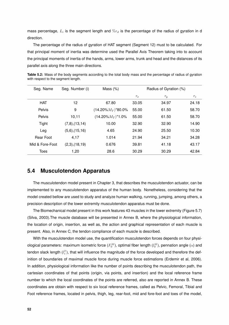
mass percentage, Li is the segment length and %rd is the percentage of the radius of gyration in d
direction.
The percentage of the radius of gyration of HAT segment (Segment 12) must to be calculated. For
that principal moment of inertia was determine used the Parallel Axis Theorem taking into to account
the principal moments of inertia of the hands, arms, lower arms, trunk and head and the distances of its
parallel axis along the three main directions.
Table 5.2: Mass of the body segments according to the total body mass and the percentage of radius of gyrationwith respect to the segment length.
Seg. Name Seg. Number (i) Mass (%) Radius of Gyration (%)
rx ry rz
HAT 12 67.80 33.05 34.97 24.18
Pelvis 9 (14.20%MT )*80.0% 55.00 61.50 58.70
Pelvis 10,11 (14.20%MT )*1.0% 55.00 61.50 58.70
Tight (7,8),(13,14) 10.00 32.90 32.90 14.90
Leg (5,6),(15,16) 4.65 24.90 25.50 10.30
Rear Foot 4,17 1.014 21.94 34.21 34.28
Mid & Fore-Foot (2,3),(18,19) 0.676 39.81 41.18 43.17
Toes 1,20 28.6 30.29 30.29 42.84
5.4 Musculotendon Apparatus
The musculotendon model present in Chapter 3, that describes the musculotendon actuator, can be
implemented to any musculotendon apparatus of the human body. Nonetheless, considering that the
model created bellow are used to study and analyze human walking, running, jumping, among others, a
precision description of the lower extremity musculotendon apparatus must be done.
The Biomechanical model present in this work features 43 muscles in the lower extremity (Figure 5.7)
(Silva, 2003).The muscle database will be presented in Annex B, where the physiological information,
the location of origin, insertion, as well as, the action and graphical representation of each muscle is
present. Also, in Annex C, the tendon compliance of each muscle is described.
With the musculotendon model use, the quantification musculotendon forces depends on four physi-
ological parameters: maximum isometric force (FM0 ), optimal fiber length (lM0 ), pennation angle (α) and
tendon slack length (lTs ), that will influence the magnitude of the force developed and therefore the def-
inition of boundaries of maximal muscle force during muscle force estimations (Erdemir et al, 2006).
In addition, physiological information like the number of points describing the musculotendon path, the
cartesian coordinates of that points (origin, via points, and insertion) and the local reference frame
number to which the local coordinates of the points are referred, also are reported in Annex B. These
coordinates are obtain with respect to six local reference frames, called as Pelvic, Femoral, Tibial and
Foot reference frames, located in pelvis, thigh, leg, rear-foot, mid and fore-foot and toes of the model,
52

where the origin matches the centre of mass of each rigid body, and orientated as shown in Figure 5.6
Figure 5.6: Location and orientation of the local reference frames. Image Retrieved from OpenSim (Delp et al,2007)
For the muscle path fits the biomechanical model and thereafter the subject under analysis, the
physiological information provided will be scaled taking into account the reference body segments length
of the subject, i.e., the pelvis height, the thigh, the leg and the foot length. The optimal fiber length and
the tendon slack length were scaled with the length of the segment that the correspondent muscle cover
more. For the muscle path the coordinates of origin, insertion and via points were scaled taking into
account the length of the segment where the correspondent point insert.
Beside the scaling, some adjustment had to be made in the database to obtain the results consistent
with physiological values. First, the tendon slack length of the quadriceps femoris group that include
the rectus femoris, vastus lateralis, medialis and intermedius, was increased in order to considerer the
patellar tendon so that those values are consistent with the muscle path given by the via points. To each
muscle was added 0.1046 m to the LTs , corresponding to 0.0394 m of patellar length and 0.0652 m of
patellar tendon length (Yamaguchi and Zajac, 1989). Also, the via point that was associated with the
thigh was removed is these muscle to obtain a physiological muscle path.
Second and last, the via and insertion points of the flexor digitorum longus and the flexos hallucis
longus associated with the foot segment was adjusted in z-coordinate to guarantee that both points
are inserted in the sole of the foot and the respective action of both muscle in the movement. This
adjustment came for the needed of adopt the database to a foot that is described with three segments
instead of one.
53

Figure 5.7: Muscle Apparatus Representation. Cyan muscle: Gluteus maximus; Green Muscle: Semitendinosus,Semimembranosus, Biceps Femoris; Black muscle: Rectus Femoris, Vastus intermedius, medialis and lateralis; Or-ange muscle: Tibialis Anterior; Blue Muscle: Gastrocnemius Medial and Lateral, Soleus, Tibialis Posterior; magentamuscle: Iliacus, Psoas.
54

6Experimental Procedure
Contents
6.1 Acquisition Protocol . . . . . . . . . . . . . . . . . . . . . . . . . . . . . . . . . . . . . 56
6.2 Data Treatment Protocol . . . . . . . . . . . . . . . . . . . . . . . . . . . . . . . . . . . 58
55
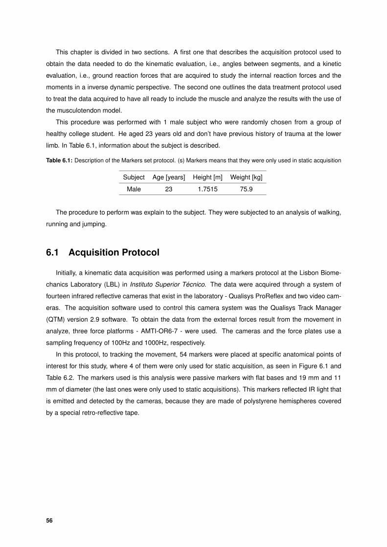
This chapter is divided in two sections. A first one that describes the acquisition protocol used to
obtain the data needed to do the kinematic evaluation, i.e., angles between segments, and a kinetic
evaluation, i.e., ground reaction forces that are acquired to study the internal reaction forces and the
moments in a inverse dynamic perspective. The second one outlines the data treatment protocol used
to treat the data acquired to have all ready to include the muscle and analyze the results with the use of
the musculotendon model.
This procedure was performed with 1 male subject who were randomly chosen from a group of
healthy college student. He aged 23 years old and don’t have previous history of trauma at the lower
limb. In Table 6.1, information about the subject is described.
Table 6.1: Description of the Markers set protocol. (s) Markers means that they were only used in static acquisition
Subject Age [years] Height [m] Weight [kg]
Male 23 1.7515 75.9
The procedure to perform was explain to the subject. They were subjected to an analysis of walking,
running and jumping.
6.1 Acquisition Protocol
Initially, a kinematic data acquisition was performed using a markers protocol at the Lisbon Biome-
chanics Laboratory (LBL) in Instituto Superior Tecnico. The data were acquired through a system of
fourteen infrared reflective cameras that exist in the laboratory - Qualisys ProReflex and two video cam-
eras. The acquisition software used to control this camera system was the Qualisys Track Manager
(QTM) version 2.9 software. To obtain the data from the external forces result from the movement in
analyze, three force platforms - AMTI-OR6-7 - were used. The cameras and the force plates use a
sampling frequency of 100Hz and 1000Hz, respectively.
In this protocol, to tracking the movement, 54 markers were placed at specific anatomical points of
interest for this study, where 4 of them were only used for static acquisition, as seen in Figure 6.1 and
Table 6.2. The markers used is this analysis were passive markers with flat bases and 19 mm and 11
mm of diameter (the last ones were only used to static acquisitions). This markers reflected IR light that
is emitted and detected by the cameras, because they are made of polystyrene hemispheres covered
by a special retro-reflective tape.
56
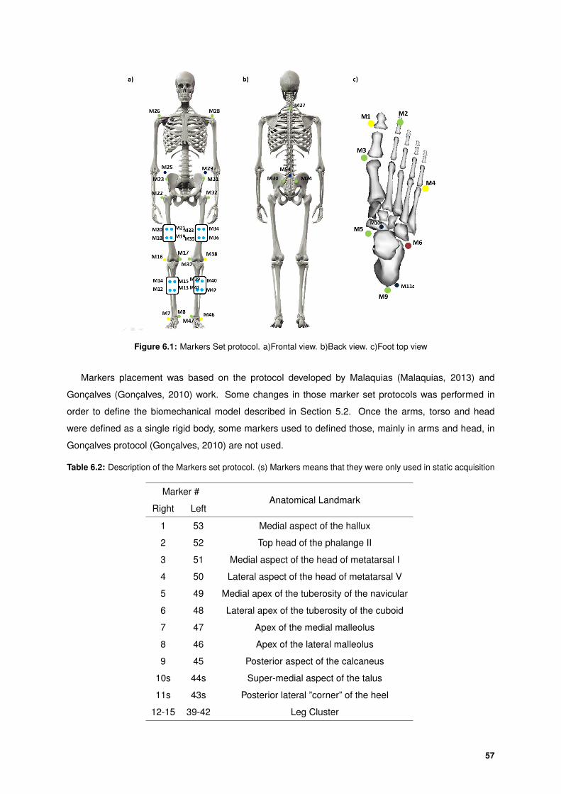
Figure 6.1: Markers Set protocol. a)Frontal view. b)Back view. c)Foot top view
Markers placement was based on the protocol developed by Malaquias (Malaquias, 2013) and
Goncalves (Goncalves, 2010) work. Some changes in those marker set protocols was performed in
order to define the biomechanical model described in Section 5.2. Once the arms, torso and head
were defined as a single rigid body, some markers used to defined those, mainly in arms and head, in
Goncalves protocol (Goncalves, 2010) are not used.
Table 6.2: Description of the Markers set protocol. (s) Markers means that they were only used in static acquisition
Marker #Anatomical Landmark
Right Left
1 53 Medial aspect of the hallux
2 52 Top head of the phalange II
3 51 Medial aspect of the head of metatarsal I
4 50 Lateral aspect of the head of metatarsal V
5 49 Medial apex of the tuberosity of the navicular
6 48 Lateral apex of the tuberosity of the cuboid
7 47 Apex of the medial malleolus
8 46 Apex of the lateral malleolus
9 45 Posterior aspect of the calcaneus
10s 44s Super-medial aspect of the talus
11s 43s Posterior lateral ”corner” of the heel
12-15 39-42 Leg Cluster
57

Continuation of Table 6.2
16 38 Most prominent point of lateral femoral epicondyle
17 37 Most prominent point of medial femoral epicondyle
18-21 33-36 Thigh Cluster
22 32 Center of acetabulum
23 31 Asis
24 30 Psis
25 29 Belly
26 28 Clavicle-acromion
27 Spinous process of C7
54 Belly Back
6.2 Data Treatment Protocol
The data acquired in the laboratory must be processed in order to perform a kinematic and kinetic
analysis. Through QTM software a .tsv file, i.e. a table-separated value file, is obtained with the markers
trajectory that were acquired. The markers were identify depending on their location to define an Auto-
matic Identification of Markers (AIM) to guarantee an efficient assignment of the trajectories. Each file
contain the trajectory corresponding to a cycle of analysis, initial contact of the foot with the force plate
for the gait and run and preparation phase, corresponding to the moment when the center of mass of
the subject descends to the ground for the jump.
A routine in Matlab was developed to treat the data. Fist, a third order low pass digital Butterworth
filter with a cut frequency of 6Hz for the gait and run, and 10 Hz for the jump was applied. It is important
for this step have at least 10 frames before and after the cycle under analysis to be discarded and to
perform a correct filtering.
After filtering, a set of steps had to be followed to create a modulation (.mdl), simulation (.sml), data
(.dat) and forces (.frc) files, needed to perform a inverse dynamic analysis. The following chapters will
explain the ones adopt to determined the variables needed to each file.
6.2.1 Modulation File
The modulation file describes the masses, inertias (Table 5.2), local coordinates of the points related
to the mass center (Table 5.1) and of the unit vectors that defines each rigid body of the biomechanical
model. Also contains the parameters that define the drivers that guide each DOF, the inner product and
superpositions constraints and the muscle apparatus (Annex B).
Through markers position, the joint centers and unit vectors coordinates were determined. Consid-
ering Figure 6.1, a formula use to determine each point and unit vectors will be describe in Table 6.3
and Table 6.4, respectively.
58

Table 6.3: Joint centers that describe the Biomechanical model. Mi represent the coordinates of the respectivemarker. The formulas present only takes into account the markers of the right, but the procedure to left one is thesame.
Pi Formula Pi Formula
P1 M∗2 P8M7+M8
2
P2 ≡ P3M3+M4
2 P9 ≡ P10M16+M17
2
P4 ≡ P5M5+M6
2 P11 ≡ P12 M22,M32,M23,M31,M54
P6 M9 P14M25+M29
2
P7M10s+M11s
2 P15M25+M28
2
Note: M∗2 is constitute by the x,y coordinates of M2 and by the z coordinate of M1
The hip joint center (P11 ≡ P12 and P13 ≡ P17) was determined through the algorithm developed by
Davis et al (Davis et al, 1991). This algorithm consist in determine the distance of the hip joint center
relative to the center of the embedded coordinate system of the pelvis obtained thought at least three
non-collinear markers attached to it, the markers positioned in ASIS, PSIS and belly back.
Table 6.4: Vectors that describe the model. The formulas present only takes into account the markers of the right,but the procedure to left one is equal. All the vector were normalized
Description Segment iKinematic Vectors Unit Vectors
Formula(Global RF) (Local RF)
HAT12
vShoulder M26 −M28
zHAT P15 − P14
xHAT v27 (zHAT × vShoulder)
yHAT v14 (zHAT × xHAT )
Pelvis 10,11
vPelvis P17 − P11
xPelvis1 v11, v12, v15, v16 xThigh1
yPelvis1 (xPelvis1 × vPelvis)
zPelvis1 vPelvis
Pelvis 9
vzPelvis P14 − P17+P11
2
xPelvis v13 (vPelvis × vzPelvis)
yPelvis v29 vPelvis
zPelvis v28 (xPelvis × yPelvis)
Thigh 8,14
zThigh1 P9 − P11
xThigh1 (vPelvis × zThigh1)
yThigh1 (zThigh1 × xThigh1)
Thigh7,13
vKnee v10, v8, v17, v19 M16 −M17
zThigh2 P9 − P11
xThigh2 (zThigh2 × vKnee)
yThigh2 (zThigh2 × xThigh2)
59

Continuation of the Table 6.4
Leg 6,16
vTalocrural v6, v20 M8 −M7
zLeg1 P9 − P8
xLeg1 (xLeg1 × vKnee)
yLeg1 (zLeg1 × xLeg1)
Leg 5,15
vMidtarsal M6 −M5
zLeg2 P9 − P8
xLeg2 v7, v18 (zLeg2 × vMidtarsal)
yLeg2 (zLeg2 × xLeg2)
Rear-foot 4,17
vTalocalcaneal v5, v22, v22 M10s −M11s
xRFM5+M6
2 −M9
zRF (vMidtarsal × xRF )
yRF v4, v21 (zRF × xRF )
Mid- & Fore-foot 2,19
vMetatarsophalangeal v1, v2, v25, v23 M4 −M3
xMFFF1 P3 − P4
zMFFF1 (vMetatarsophalangeal × xMFFF1)
yMFFF1 (zMFFF1 × xMFFF1)
Mid- & Fore-foot 3,18
xMFFF2 P3 − P4
zMFFF2 v3, v24 (vMidtarsal × xMFFF2)
yMFFF2 (zMFFF2 × xMFFF2)
Toes1,20
xToes M∗2 − M3+M4
2
zToes v9, v26 (vMetatarsophalangeal × xToes)
yToes (zToes × xToes)
The transformation of the vectors from global reference frame to local reference frame was performed
through Equation 6.1.
vLFi = A−1vGFi (6.1)
Where vLFi and vGFi are the vectors in the local and global reference frame, respectively, and A−1 is
the transformation matrix that is composed by the vectors that define the local reference of a rigid body
(Equation 6.2), determined in Table 6.4.
A = [xTRB yTRB zTRB ] (6.2)
RB is the respective rigid body.
6.2.2 Simulation File
The simulation file presents the initial state of the system, i.e., positions, velocities, Tait-Bryan angles
and angular velocity of each rigid body, related to the center of mass in the global reference frame. Also,
60

addressed the time parameters, the gravity field vector and the optimization procedure definition.
The positions coordinates are obtained through the relation present in Equation 6.3.
PRBCM = Pi +Asi (6.3)
PRBCM is the coordinates of center of mass in the global reference frame of rigid body RB, Pi is the
coordinates in the global reference frame of a joint center i that defines the rigid body, obtained in Table
6.3, A is the transformation matrix and si is the position of the joint center i related to the center of mass
in the local reference frame (Table 5.1).
The Tait-Bryan angles with a sequence of rotation Z-Y-X will described the orientation of the seg-
ments. The sequence of rotation defines the order of rotation about the axis. First the segment will
suffer a positive rotation φ about the z-axis, second a positive rotation θ about the y’-axis and finally, a
positive rotation ψ about the x”-axis, resulting in the final system (Laananen el al, 1983). Through the
matrix (Equation 6.4) that results of these sequence and the transformation matrix obtained above the
orientation of the segments was achieved.
A =
cos(θ) cos(φ) sin(ψ) sin(θ) cos(φ)− cos(ψ) sin(φ) cos(ψ) sin(θ) cos(φ) + sin(ψ)cos(φ)
cos(θ) sin(φ) cos(ψ) sin(θ) sin(φ)− sin(ψ) cos(φ) sin(ψ) sin(θ) sin(φ) + cos(ψ) cos(φ)
− sin(θ) sin(ψ) cos(θ) cos(ψ) sin(θ)
(6.4)
6.2.3 Data File
The data file contains the angles over time that drives the model. Each file can contain one of five
different type of drivers that were define in the modulation file: angle between one unit vector and one
segment, angle between two unit vectors, angle between two segments, global coordinates of one point
and global coordinates of a vector. Those drivers describes the DOF of the system and they were
determined through a Matlab routine developed using the following expression:
Φi = arccos(v.u
|v||u|) (6.5)
Where Φi correspond to the angle of driver i and v and u are the vectors chosen to evaluate the driver
as described in Table 6.5. This choice tries to avoid angles out of the range of [0◦ − 180◦].
61

Table 6.5: Vectors that allow the calculation of the kinematic drivers. The formulas present only takes into accountthe markers of the right, but the procedure to left one is equal.
Description Driver i Vectors
Dorsiflexion and Plantarflexion Metatarsophalangeal Joint 1 xMFFF1, zToes
Internal rotation Mid-foot & Fore-foot 2 xMFFF1, zMFFF2
Dorsiflexion and Plantarflexion Midtarsal Joint 3 xRF , zMFFF2
Abduction and Adduction Midtarsal Joint 4 −yRF , xMFFF1
Inversion and Eversion Talocalcaneal Joint 5 −yRF , zLeg
Dorsiflexion and Plantarflexion Talocrural Joint 6 vTalocrural, zLeg
Internal Rotation Leg 7 vTalocalcaneal, xLeg2
Flexion Extension Knee Joint 8 −zLeg, zThighInternal Rotation Thigh 9 xThigh1, yThigh2
Abduction and Adduction Hip Joint 10 yPelvis, −zThighFlexion Extension Knee Joint 11 xPelvis1, zPelvis
Lateral extension Pelvis Joint 12 zTronco, yPelvis
Flexion Extension Pelvis Joint 13 zTronco, xPelvis
6.2.4 Force File
The forces file contains the ground reaction forces (GRFs), the center of pressure curve (COP), the
number of forces and the rigid body where are applied in each instant of time.
This information was exported from QTM software as three *.tsv, one for each force platform, and
then treated in Matlab. The data of each platform was filtered with a third order low pass digital Butter-
worth filter with 16 Hz for gait, 40 Hz for run and 30 Hz for jump. Subsequently, the filtered data was
assigned in twelve column, six for each foot, where the first three correspond to the coordinates (x,y,z)
of the GRF’s and the other three to the coordinates (x,y,z) of COP over time.
62

7Results and Discussion
Contents
7.1 Gait Analysis . . . . . . . . . . . . . . . . . . . . . . . . . . . . . . . . . . . . . . . . . . 64
7.2 Run Analysis . . . . . . . . . . . . . . . . . . . . . . . . . . . . . . . . . . . . . . . . . . 70
7.3 Jump Analysis . . . . . . . . . . . . . . . . . . . . . . . . . . . . . . . . . . . . . . . . . 76
7.4 Discussion . . . . . . . . . . . . . . . . . . . . . . . . . . . . . . . . . . . . . . . . . . . 81
63

After the development of the musculotendon model described in Chapter 3 and the development of
biomechanical model described in Chapter 5 and 6, the results of musculotendon forces and muscle
activations were obtained. In this chapter, the results will be present and analyze in order to realize the
influence of each muscle in the different phases of the movement. Also, the results obtained through the
muscle Hill model developed by Pereira (Pereira, 2009) will be display to compare and understand the
influence of the tendon in the movement.
The results will be analyzed mainly in the sagittal plane and the muscle will be grouped according to
their most important function. Quadriceps femoris composed by the vastus medialis (VM), vastus inter-
medius (VI), vastus lateralis (VL) and rectus femoris (RF); Hamstrings composed by the semitendinosus
(ST), semimembranosus (SM), biceps femoris (long (BFLH)) and short head (BFSH)); triceps surae,
composed by soleus and the two head of the gastrocnemius (medial (GM) and lateral (GL)); ilipsoas
composed by iliacus (I) and psoas; ankle plantarflexors composed by the triceps surae, tibialis posterior
(TP) and peroneus longus (PL); and the ankle dorsiflexors composed by the tibialis anterior (TA). Some
muscle will not be included in the results due to almost no activity present in the movement analyzed.
7.1 Gait Analysis
The gait cycle, movement of the lower limbs during walking, consist of one cycle of swing and stance
phase by one limb, in this case the right one (limb represented in Figure 7.1 with red muscles). The
stance phase consists in the period where the right limb is in contact with the ground, and the swing
phase where is not (Figure 7.1).
Figure 7.1: Scheme with different phases of Gait Cycle
The stance and swing phases are divided in different events, which name are based on the movement
of the foot, that are important to describe and understand the physiological analysis that will be realize
below. The stance phase starts with the initial contact of the heel, named Heel strike (HS) at 0% of cycle.
64

Followed by the Opposite Toe Off (OTO), instant where the left leg leave the ground. At this moment, the
body passes through a mid stance at 30% of the cycle, where a progress of the body occur and the right
limb support the body weight. The stance phase end just before occur the Opposite Heel Strike (OHS),
initial contact of the left foot, and a swing phase starts, approximately at 60%, when the right limb leaves
the ground, Toe Off (TO) phase. At 80% of gait, a mid swing phase occurs, where the right limb moves
onward, ending at 100% when the HS happens again.
The results present in the figures above allow the visualization of two distinct phases of gait cycle. In
stance phase (0%− 60%), there are present high level of muscle activation and consequently of muscle
forces, which are developed to support the body weight and move the body forward. On the other hand,
in the swing phase, small levels of muscle activation and thereafter muscle forces are present. The
description of the activity of the muscle and the respective muscle force along the cycle will realize only
for the results obtained by the musculotendon model.
Taking into account the different phases of gait and analyzing the figures above, it is possible to
identify the contribution of each muscle for the movement observed. The analysis starts with the HS
where the dorsiflexors, mainly the Tibialis Anterior (TA) (Figure 7.8) and the hamstrings (Figure 7.4)
are activated. This initial activity of the dorsiflexors aims to control the landing of the calcaneus on the
surface due to the weight admitted in HS. The contraction present in the hamstring allows the weight
transfers from a single support to a double support, giving stability to the body. Also, in this initial phase,
the plantarflexors are activated. Tibialis posterior (Figure 7.7), gastrocnemius (Figure 7.2) present a
small activation to guarantee joint stabilization .
When the OTO phase occurs, the body weight is totally transferred to the right leg. Muscle activity and
consequently musculotendon force of the triceps surae (Figure 7.2) was detected to control the rotation
of the leg around the ankle and the stabilization of the ankle joint. Even before 30%, the moment when
the left foot passes a point below the left hip joint, muscle activation and consequently musculotendon
force are observed in the hamstrings and in the quadriceps femoris. This muscular activity will promote
the stabilization of the knee joint, once the right leg is supporting all the body weight.
After mid stance phase, the ankle plantarflexors develop significantly muscle force. This force is
mainly realized by the triceps surae (Figure 7.2), and it is responsible to bring the body forward. Besides,
a contraction of the quadriceps femoris (rectus femoris and vastus) (Figure 7.3) occurs close to the TO.
This muscle activity is responsible to the extension of the knee and to ensure this extension while the
impulse given by the foot is transmitted to the hip, pelvis and trunk, when there is a forward inclination
(Silva, 2003). The stance phase ends when occurs the TO, moment when the ankle plantarflexion force
decrease.
A swing phase begins now and muscle activation of the tibialis anterior (Figure 7.8) is observed.
This activity will maintain the foot in a stable position and prepare it to the next HS. During this phase,
the flexion of the hip joint must occur. Activations of the hip flexors, Psoas and iliacus (Figure 7.5), are
activated to produce that movement.
At the end of the swing phase, occur an increase activity of the hamstrings (Figure 7.4), mainly, the
biceps femoris. This muscle presents activity to decelerate the lower leg and foot, until the nearly full
65
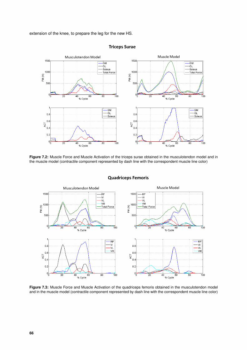
extension of the knee, to prepare the leg for the new HS.
Figure 7.2: Muscle Force and Muscle Activation of the triceps surae obtained in the musculotendon model and inthe muscle model (contractile component represented by dash line with the correspondent muscle line color)
Figure 7.3: Muscle Force and Muscle Activation of the quadriceps femoris obtained in the musculotendon modeland in the muscle model (contractile component represented by dash line with the correspondent muscle line color)
66

Figure 7.4: Muscle Force and Muscle Activation of the hamstring obtained in the musculotendon model and in themuscle model (contractile component represented by dash line with the correspondent muscle line color)
Figure 7.5: Muscle Force and Muscle Activation of the ilipsoas obtained in the musculotendon model and in themuscle model (contractile component represented by dash line with the correspondent muscle line color)
67

Figure 7.6: Muscle Force and Muscle Activation of the gluteus maximus obtained in the musculotendon model andin the muscle model (contractile component represented by dash line with the correspondent muscle line color)
Figure 7.7: Muscle Force and Muscle Activation of the tibialis posterior obtained in the musculotendon model andin the muscle model (contractile component represented by dash line with the correspondente muscle line color)
68

Figure 7.8: Muscle Force and Muscle Activation of the tibialis anterior obtained in the musculotendon model and inthe muscle model (contractile component represented by dash line with the correspondent muscle line color)
The results obtained in both models must be compared to understand the influence of the tendon in
gait. The principal difference present is the presence of passive force in the muscle model. According
to the force-length muscle relationship this means that the muscle length is longer compared with the
isometric muscle length.
In the musculotendon model, the variation of tendon length enables the muscle to work at a more op-
timal velocity vM0 and length lM0 . When muscle working in this zone, the activation needed to developed
the force required will be lower than the present in the muscle model.
In Figure 7.2, where are represented the results of triceps surae significant differences are detected.
If the muscle force obtained with the musculotendon model were compared with the contractile muscle
force obtained (dash lines with the respective color) the differences are too small, which means that the
passive force is almost nonexistent. Otherwise, when analyze the results of the muscle model, although
the muscle force produce by those muscle are greater, most of them correspond to passive force. The
muscle is then working in a non-favorable zone, when it needs more activation to obtain the contractile
force to archive to the moment desired.
In relation to the quadriceps femoris (Figure 7.3), the same conclusion can be taken in relation to
rectus femoris. Otherwise, in vastus the muscle and the contractile force are practically equal. In this
case, a clearly conclusion about the influence of the tendon cannot be performed since the optimizer
give different weights to the muscle to produce extension of the knee.
In the hamstring (Figure 7.4), the tendon, according to the results, do not have influence. The muscle
force is practically equal to the contractile force with small and not influenced differences.
69

The two models present some different in the intensity of the muscle force during the cycle. The
mainly difference found is in the semimembranosus. At 20% of the gait, this muscle present a muscle
force much higher in the musculotendon model than in the muscle model. This value occurs when the
hip is extended and the right leg support all the body weight. In the muscle model, this force is exerted
by the gluteus maximus, as seen in Figure 7.6. Since those muscles are hip extensors, both must be
working as happen in the musculotendon model.
In Tibialis Posterior (Figure 7.7), a strong passive component was obtained in the muscle model.
A clearly evidence of the influence of the tendon is present in this muscle. Comparing the contractile
force and muscle activation of the muscle model to the musculotendon model, much more activation
was needed to realize the same movement, once the muscle is not work in the optimal zone.
Finally, in Tibialis Anterior (Figure 7.8), iliacus and Psoas (Figure 7.5), the influence of the tendon is
not remarkable.
To end the discussion of the gait analysis, the results obtained was compared to the literature. The
results obtained are very similar to the ones present to the work of Crowninshield and Brand (Crownin-
shield & Brand, 1981), mainly in the gait phases where are present activation and consequently, muscle
force.
7.2 Run Analysis
Running, like walking, is an activity characterized by a cycle which repeats over time. In this analyses
the cycle beginning and end with HS. Unlike what happen in gait cycle, running only is divided into a
support phase, when a foot is on the ground and a recovery phase in which both feet are off ground.
The results present in this work are referent to the support and recovery phase of the right limb.
This only represent 55% of the running cycle (Figure 7.9), once is not observable opposite heel strike
(OHS) and the final HS of the right limb. This happens due to absence of space in the Laboratory during
acquisition of running analysis, when the the remains phase of the cycle was out of the volume detection
of the cameras.
Figure 7.9: Scheme with different phases of Running Cycle
70

As happen in gait cycle, the stance phase consist in the period where the right limb is in contact with
the ground, and the swing phase where is not. Both phases are divided in different events, which name
are based on the movement on the foot.
The stance phase starts, in this case, with a heel contact and it is followed by a mid stance phase
(30%), when the right limb support all the body weight and occur the forward progressing of the body.
This phase ends with TO and the swing phase begins with double float, no foot is in contact with the
ground.
Through the results obtained (Figure 7.10 to Figure 7.16), high levels of muscle activation and con-
sequently the muscle forces are present in the stance phase, as expected. Between the 40% and 55%,
double float phase, there is a decrease of those levels. The description of the activity of the muscle and
the respective muscle force along the cycle will realize only for the results obtained by the musculotendon
model.
After the HS and before the mid stance phase occurs a period of absorption. In this period the body’s
center of mass decrease and its velocity decelerates horizontally (Hamner & Delp, 2010). Analyzing
Figure 7.11, Figure 7.14 and Figure 7.12 strong muscle activity is present in the knee (quadriceps
femoris) and hip extensors (gluteus maximus and hamstring). Quadriceps femoris are activated in this
period to prepare the limb for the ground contact and to absorb the shock of the impact. The hip
extensors, gluteus maximus and the hamstring, mainly the semimembranosus, also present high levels
of activations to contribute to the body support. The activation of these muscles, together with the triceps
surae, will provide the acceleration of the body vertically until the mid stance.
Forward propulsion of the body in this phase is provided initially by hip extensors discussed above,
and after mid stance by the ankle plantarflexors, soleus, gastrocnemius (GM, GL) (Figure 7.10) and
peroneus longus (Figure 7.15).
In the beginning of the swing phase, tibialis anterior (Figure 7.16), iliacus and psoas (Figure 7.13)
are activated to prepare the foot for the next HS, and to flex the hip joint, respectively.
During double float phase, occurs an increase activity of the hamstrings (Figure 7.12) to decelerate
the lower leg and foot and preparing to the new HS.
Comparing the two models, some differences are also found. Starting with the triceps surae (Figure
7.10), the presence of a tendon improves the results. The muscles work in optimal zone allowing the
production of more force with less activation. In the results of the muscle model, the muscle force are
mainly compose by a passive component and the muscle activation are at the same levels compare to
the other model, but the contractile force produce is almost zero. Also, the gastrocnemius, either the
medial or the lateral, should be active until the TO and not after as happen in the Muscle model. The
contraction of those muscles before the TO is very important to bring the body forward.
71

Figure 7.10: Muscle Force and Muscle Activation of the triceps surae obtained in the musculotendon model and inthe muscle model (contractile component represented by dash line with the correspondent muscle line color)
Figure 7.11: Muscle Force and Muscle Activation of the quadriceps femoris obtained in the musculotendon modeland in the muscle model (contractile component represented by dash line with the correspondent muscle line color)
72

Figure 7.12: Muscle Force and Muscle Activation of the hamstring obtained in the musculotendon model and in themuscle model (contractile component represented by dash line with the correspondent muscle line color)
Figure 7.13: Muscle Force and Muscle Activation of the ilipsoas obtained in the musculotendon model and in themuscle model (contractile component represented by dash line with the correspondent muscle line color)
73

Figure 7.14: Muscle Force and Muscle Activation of the gluteus maximus obtained in the musculotendon modeland in the muscle model (contractile component represented by dash line with the correspondent muscle line color)
Figure 7.15: Muscle Force and Muscle Activation of the tibialis posterior and peroneus longus obtained in the mus-culotendon model and in the muscle model (contractile component represented by dash line with the correspondentmuscle line color)
74

Figure 7.16: Muscle Force and Muscle Activation of the tibialis anterior obtained in the musculotendon model andin the muscle model (contractile component represented by dash line with the correspondent muscle line color)
As happen in gait analysis, in the quadriceps femoris (Figure 7.11) only the rectus femoris has
significant passive components, mainly in the double float phase. In vastus medialis and intermedius,
the influence of the tendon is verified. It is notable in Figure 7.11 that with lower values of muscle
activation, the muscle is producing more muscular force. Although in the results of the vastus lateralis
does not exist almost passive component, the change of the tendon length improve the results, once
only with the double of muscle activation, the muscle produce a muscle force six time more comparing
the two models.
Finally, the rectus femoris is more active when using musculotendon model. Since, in the stance
phase these muscles are responsible to absorb the force of impact it is expected a muscle force high.
In Hamstring (Figure 7.12) the same conclusions can be taken. In the beginning the swing phase, the
force developed by the semimembranosus is completely influence by the change of the tendon length.
The passive component is low, and the force developed is very high when analyzed the muscle activation
obtained. Analyzing, the double float phase, the something happens with the semitendinosus and with
biceps femoris long head.
Observing the result obtained for ilipsoas (Figure 7.13), the passive component is almost zero and it
is not evident the influence of the tendon. The same happens with tibialis anterior.
In gluteus maximus (Figure 7.14), only is notable the presence of the tendon in the posterior. Finally,
the tibialis posterior (Figure 7.15) where also the some conclusions can be taken.
Compared the results obtained with the ones presents in the Hamner and Delp work (Hamner &
Delp, 2010), correlation in the zone where the muscle are activated during the cycle are found.
75

7.3 Jump Analysis
Jumping is divided biomechanically into three phases: preparation, action and recovery (Bartlett,2007)
(Figure 7.17). The first one is characterize as the lowering phase, which positioning the body for the ac-
tion phase and stores elastic energy in the eccentrically contracting muscle. The action phase is featured
by a upper phase until feet leave the floor, where both knee joints extending or plantarflexing together.
The recovery phase involves the air and controlled landing, through, in the last one, eccentric contraction
of the leg muscles.
Figure 7.17: Scheme with different phases of Jumping Cycle
In the preparation phase, occur the flexion of the hip and knee and the dorsiflexion of the ankle. To
allow this movements the hamstrings (semimembranosus, semitendinosus and biceps femoris) (Figure
7.20), and the hip flexors, mainly rectus femoris (RF) (Figure 7.19), ilipsoas (Figure 7.21), contract.
The action phase involves the hip and knee extension and the ankle plantarflexion through contrac-
tion of the muscle responsible for that movement driving the body vertically upwards. Analyzing the
results obtained, the hip extensors (bicep femoris, semitendinosus, semimembranosus (Figure 7.20)
and gluteus maximus (Figure 7.22) present muscle activity and consequently muscle force that enable
the movement. The quadriceps femoris are activated to promote the knee extension and the gastrocne-
mius, soleus (Figure 7.18), peroneus longus, tibialis posterior (Figure 7.23) are also activated to enable
the plantarflexion.
In the air phase, the muscle activity observed is must lower than the remain cycle. In landing phase
(75% of cycle), a great activity is observed in quadriceps femoris (Figure 7.19) and gluteus maximus
(Figure 7.22) to stabilize knee and pelvis joints, respectively. The muscle force realize by the quadriceps
femoris (Figure 7.19) during landing is higher than in the impulse phase. In Annex D, (Jump analysis
figure), where the force in z direction realize in force platform is represented, it is possible to observed
that the force realize it conform the results observed.
The integration of the tendon in the model also influences the results in the jump but passive force
is now present in both models due to the type of movement. Analyzing the results obtained by the two
76

models, the same conclusions already taken in the previous section could be made for the triceps surae
(Figure 7.18), gluteus maximus (Figure 7.22), ilipsoas (Figure 7.21), tibialis posterior and peroneus
longus (Figure 7.23). The quadriceps femoris constitute the set of muscles that present a significant
passive component, but it do not influence the differences found in the two models in the contractile
force and muscle activation when compared.
The results obtained for the hamstring (Figure 7.20) feature many differences in order to be able to
conclude over the benefits of the tendon.
Finally, in tibialis anterior (Figure 7.24), once again, the integration of the tendon is not remarkable.
The activity of this muscle is much higher in the muscle model in the air phase. The excessive activity
present in the tibialis anterior using the muscle model it is to compensate the excessive passive compo-
nent that occurs in the plantarflexors, mainly the peroneus longus, in the same phase of the movement.
Taking into account the literature (Spagele et al, 1998), a correlation of the phases where the muscle
are activates is clearly present.
Figure 7.18: Muscle Force and Muscle Activation of the triceps surae obtained in the musculotendon model and inthe muscle model (contractile component represented by dash line with the correspondent muscle line color)
77

Figure 7.19: Muscle Force and Muscle Activation of the quadriceps femoris obtained in the musculotendon modeland in the muscle model (contractile component represented by dash line with the correspondent muscle line color)
Figure 7.20: Muscle Force and Muscle Activation of the hamstring obtained in the musculotendon model and in themuscle model (contractile component represented by dash line with the correspondent muscle line color)
78

Figure 7.21: Muscle Force and Muscle Activation of the ilipsoas obtained in the musculotendon model and in themuscle model (contractile component represented by dash line with the correspondent muscle line color)
Figure 7.22: Muscle Force and Muscle Activation of the gluteus maximus obtained in the musculotendon modeland in the muscle model (contractile component represented by dash line with the correspondent muscle line color)
79

Figure 7.23: Muscle Force and Muscle Activation of the tibialis posterior and peroneus longus obtained in the mus-culotendon model and in the muscle model (contractile component represented by dash line with the correspondentmuscle line color)
Figure 7.24: Muscle Force and Muscle Activation of the tibialis anterior obtained in the musculotendon model andin the muscle model (contractile component represented by dash line with the correspondent muscle line color)
80

7.4 Discussion
Analysing the results obtained in the three movements study, concludes that the importance of the
tendon depends on the muscle and on the type of movement. The presence of the tendon in triceps
surae and tibialis posterior interfere in the results in the gait, run and jump. Unlike what happens with
the tibialis anterior, the implementation of the musculotendon model is not remarkable. In ilipsoas and
quadriceps femoris, differences found are more significantly in jump than in gait or run.
Concluding, the use of model that includes the behavior of the tendon in the analysis of movement
is important in all type of movement. With the implementation of the musculotendon model developed in
this thesis, the results obtained are physiologically more real even when the presence of the tendon is
no significantly, like in TA.
81

82

8Conclusions and Future
Developments
Contents
8.1 Conclusions . . . . . . . . . . . . . . . . . . . . . . . . . . . . . . . . . . . . . . . . . . 84
8.2 Future Developments . . . . . . . . . . . . . . . . . . . . . . . . . . . . . . . . . . . . . 84
83
8.1 Conclusions
The objectives propose for this work was successfully fulfilled. A valid musculotendon model was
developed within the framework of multibody systems dynamics and a biomechanical model composed
by 43 muscle actuators was created in order a study the influence of the tendon in diverse types of
activity, like walking, running and jumping.
In order to achieved those objective, some topics had to be addressed. In chapter 2, the anatomy and
physiology of the muscle and tendon was described in order to understand the behaviour of this complex
during movement and to understand the mechanical properties implemented in the model described in
chapter 3.
Once, the musculotendon model was implemented within the framework of multibody system dy-
namics in natural coordinates, in chapter 4 the multibody dynamics formulation was described. Also,
the model implementation in a forward and inverse perspective was explained and an simple example
of flexion of the elbow was realize in order to validate and understand the functioning of the model.
To analyze the model developed in walking, running and jumping, a biomechanical model of the
whole body was developed. In chapter 5, all the steps needed to developed this model was described,
as well as, the muscle apparatus of the lower limb implemented was analyzed.
To obtained the results for a inverse dynamic perspective, an acquisition protocol was developed to
acquired the data needed. Chapter 6 therefore explains the acquisition protocol adopted and all the
steps followed to treat the data and to create the files needed to implemented the model.
Finally, in chapter 7 the results obtained are present and discuss. Analyzing the results obtained
along the cycle, the muscle activities and the muscle force obtained are consistent with the movement
observed. When compared this model with the muscle model, the influence of the tendon is evident in
all the analyses. The main differences are the percentage of passive component in certain moments of
the cycle, and the intensity of the muscle force realizes taking into to account the activity present. The
changing on tendon length allow the muscle to contract or elongate with a length and velocity more close
to the optimal one, decreasing the activation needed to produce the force to realize a certain movement.
Although, in some muscle the presence of the tendon is not so significant, it is important to considerer
tendon in the models to guarantee that results for other muscles are more physiological and more close
to the reality, and to study which are the muscles where the tendon is important to realize a specific
activity.
8.2 Future Developments
Considering the work realize in this thesis there are some issues that could be studied to improved
the results obtained in this thesis.
Obstacle Set Method
Musculoskeletal geometry is very important to obtained physiological results relatively to the muscle
84

function. The path of the muscle will determine the moment arm and therefore the moment about
the joint and the musculotendon length for a specific body position. With the introduction of obstacle set
methods, the shape of the joint will change, allowing the muscle to slide freely over the bones and others
muscle and to produce smooth moment arm-joint angle curve. The muscle path will be not constrained
by contact with other muscles and bone, improving the results obtained for the musculotendon forces.
Muscle Optimization
The muscle optimization is one of the most important steps to obtained the results for the muscle
activations for the movements analyzed. The routine use in this work have a lower computational effi-
ciency, taking more than seven hours to run. Also, the results obtained have a bit of noise which difficult
the analyze. An alternative is the use of DNCONG, a routine of optimization of IMSL Library devel-
oped by Visual Numerics, INC, to solve a general nonlinear programming, by means of a successive
quadratic programming algorithm and a user-supplied gradient (IMSL, 1997). The routine developed
in the more recent library was improved allowing to change certain parameters that made this a very
sensitive routine to converge when the local-minima determined ir far for the optimal solution.
Laboratory Acquisition
In the Laboratory, a continue study of non-pathological subjects must be done in order to increase
the number of pattern subjects. Also, the beginning of the study of pathological subjects to understand
the influence of tendon in certain pathologies. The results obtained may be useful, as said in previ-
ous captions, to develop corrective biomedical devices, as prosthetic, orthotic designed and functional
neuromuscular stimulation systems to restore lost os impaired motor function.
The acquisition of the data for running could be realize in a crosswalk in order to acquired the entire
cycle. Also, this model can be use to analyze other activities and to improve sports performance.
85

86

References
Ackermann, M. (2007). Dynamics and energetics of walking with prostheses (PhD Thesis). University
of Stuttgart.
Amirouche, F. (2006). Fundamentals of Multibody Dynamics: Theory and Applications. Chicago.
Anderson,C. (2007). Equations for modelling the forces generated by muscle and tendons. Physics-
based Simulation of Biological Structures.
Anderson, F. C., & Pandy, M. G. (1999). A Dynamic Optimization Solution for Vertical Jumping in
Three Dimensions. Computer Methods in Biomechanics and Biomedical Engineering, 2(3), 201-231.
doi:10.1080/10255849908907988
Anderson, F. C., & Pandy, M. G. (2001). Dynamic Optimization of Human Walking. Journal of
Biomechanical Engineering, 123(5), 381. doi:10.1115/1.1392310
Bartlett, R. (1997). Introduction to Sports Biomechanics. Abingdon, UK: Taylor & Francis.
doi:10.4324/9780203476161
Buchanan, T. S., Lloyd, D. G., Manal, K., & Besier, T. F. (2005). Estimation of Muscle Forces and
Joint Moments Using a Forward-Inverse Dynamics Model. Medicine & Science in Sports & Exercise,
37(11), 1911-1916. doi:10.1249/01.mss.0000176684.24008.6f
Buchanan, T. S., Lloyd, D. G., Manal, K. & Besier, T.F. (2006). Neuromusculoskeletal modelling:
estimation of muscle forces and joint moments and movements from measurements of neural
command. Journal Application Biomechanic. 20(4), 367-395.
Crowninshield, R. D. & Brand, R.A. (1981). A Physiologically based criterion of muscle force in
locomotion. Journal of Biomechanics. 14(11),793-801. doi:0021-9290/81/110793-09
Davis III, R.B., Ounpuu, S., Tyburski, D. and Gage, J. (1991). A gait analysis data collection and
reduction technique. Human Movement Science, 10, 575-587.
Delp, S. L., & Loan, J. P. (1995). A graphics-based software system to develop and analyze models
of musculoskeletal structures. Computers in Biology and Medicine, 25(1), 21-34. Retrieved from
http://www.ncbi.nlm.nih.gov/pubmed/7600758
87

Delp, S. L., Loan, J. P., Hoy, M. G., Zajac, F. E., Topp, E. L. & Rosen, J. M. (1990). An interactive
graphic-based model of lower extremity to study orthopaedic surgical procedures. IEEE Transactions
on Biomedical Engineering. 37(8), 757-767.
Delp, S. L., Anderson, F. C., Arnold, A. S., Loan, P., Habib, A., John, C. T., . . . Thelen, D. G. (2007).
OpenSim: open-source software to create and analyze dynamic simulations of movement. IEEE
transactions on bio-medical engineering, 54(11), 1940-50. doi:10.1109/TBME.2007.901024
DeWoody YSSA, B. S. & M.S. (1998). The role of musculoskeletal dynamics and neuromuscular
control in stress development in bone. Dissertation in Mathematics, Faculty of Texas Tech University
Erdemir, A., McLean, S., Herzog, W., & van den Bogert, A. J. (2007). Model-based estimation of
muscle forces exerted during movements. Clinical Biomechanics (Bristol, Avon), 22(2), 131-54.
doi:10.1016/j.clinbiomech.2006.09.005
Guyton, A. C., & Hall, J. E. (1956). Textbook of Medical Physiology. (J. E. Hall, Ed.) (11th ed.).
Philadelphia, PA: Elsevier.
Jacobs, D.A., (2013).First-Order Activation Dynamics OpenSim. Retrieved August 14, 2014, from
http://simtk-confluence.stanford.edu:8080/display/OpenSim/First-Order+Activation+Dynamics
Goncalves, S. M. (2010). Advanced Computer Methods for Pathological and Non-Pathological Human
Movement Analysis (MSc Thesis). Instituto Superior Tecnico - Universidade Tecnica de Lisboa
Hirashima, M., Ohgane, K., Kudo, K., Hase, K. & Ohtsuki, T. (2003). Counteractive Relationship
Between the interaction torque and muscle torque at the wrist is predestined in ball-throwing. Journal
Neurophysiol. 90, 1449-1463.
Hoy, M. G., Zajac, F. E. & Gordon, M. E. (1990). A musculoskeletal model of the human lower
extremity: the effect of muscle, tendon, and moment arm on the moment-angle relationship of
musculotendon actuators at the hip, knee, and ankle. Journal of Biomechanics. 23(2), 157-169
Hamner, S. R., Seth, A. & Delp, S. L. (2010). Muscle contributions to propulsion and support during
running. Journal of Biomechanics. 43, 2709-2716. doi:10.1016/j.jbiomech.2010.06.025
IMSL. (1997) Fortran Subroutines for mathematical Applications. Visual Numerics. Volume 2.
Jalon, J. G., & Bayo, E. (1994). Kinematic and Dynamic Simulation of Multibody Systems: The real
time challenge. New-York, NY: Springer-Verlag.
Johnson, D. & Pedowitz, R. (2006). Pratical Orthopaetic Sports Medicine and Arthroscopy. Phyladel-
phia, Lippincott Williams & Wilkins
Laananem, D. H., Bolukbasi, A. O. And Coltman J. W. (1983). Computer Simulation of an aircraft seat
and occupant in a crash environment, 1.
88

Lorens, T &, Campello, M. Biomechanics of skeletal muscle. 6.
Magnusson, S. P., Narici, M. V, Maganaris, C. N., & Kjaer, M. (2008). Human tendon behaviour and
adaptation, in vivo. The Journal of Physiology, 586(1), 71-81. doi:10.1113/jphysiol.2007.139105
Malaquias, T. M. (2013). Development of a Three-Dimensional Multibody Model of the human leg
and foot for application to movement analysis (MSc Thesis). Instituto Superior Tecnico - Universidade
Tecnica de Lisboa.
Manal, K. T., & Buchanan, T. S. (2004). Biomechanics of Human Movement. Standard handbook of
biomedical engineering and design. 5, 1-26.
Martin, C. F., & Schovanec, L.. The Control and Mechanics of Human Movement Systems, (003644),
1-30.
Millard, M., Uchida, T., Seth, A., & Delp, S. L. (2013). Flexing computational muscle: modeling and
simulation of musculotendon dynamics. Journal of Biomechanical Engineering, 135(2), 021005.
doi:10.1115/1.4023390
Muscle-Tendon Mechanics (2014). Retrieved August 13, 2014, from
http://www.chrisevans3d.com/files/reference/muscle tendon mechanics milner.pdf
Neptune, R. R., & Kautz, S. a. (2001). Muscle activation and deactivation dynamics: the governing
properties in fast cyclical human movement performance? Exercise and Sport Sciences Reviews,
29(2), 76-80. Retrieved from http://www.ncbi.nlm.nih.gov/pubmed/11337827
Neurobiology (2014). Retrieved August 11, 2014, from http://www.learner.org/courses/biology
/textbook/neuro/neuro 4.html
Oatis (2014). Retrieved August 16, 2014, from http://downloads.lww.com/wolterskluwer vitalstream
com/sample-content/9780781774222 Oatis/samples/Oatis CH04 045-068.pdf
Pandy, M. G. (2001). Computer modeling and simulation of human movement. Annual review of
biomedical engineering, 3, 245-273.
Pandy, M. G., & Barr, R. E. (2004). Biomechanical of the Musculoskeletalo system. Standard
handbook of biomedical engineering and design. 6, 1-34.
Pereira, A. F. (2009). Development of a Hill-Type Muscle Model With Fatigue for the Calculation of
the Redundant Muscle Forces using Multibody Dynamics (MSc Thesis). Instituto Superior Tecnico -
Universidade Tecnica de Lisboa.
Qualisys AB. (2013). Qualisys Track Manager User Manual.
Raison, M. (2009). On the quantification of joint and muscle efforts in the human body during motion
(PhD Thesis). Ecole Polytechnique de Louvain, Uiniversite Catholique de Louvain.
89

Robleto, R. A. (1997). An Analysis of the musculotendon dynamics of hill-based models (MSc
Thesis). Faculty of Texas Tech University.
Salinas-avila, A., & Moreno-valenzuela, J. (2009). Switched Control of Mechanical Systems by Using
Musculotendon, 331-336.
Scheepers, F., Parente, R. E., Carlson, W.E. & May, S. F. (1970). Anatomy-Based Modeling of the
Human Musculature.
Scott, W., Stevens, J. & Binder-Macleod, S.A. (2001). Human Skeletal Muscle Fiber Type classifica-
tions. 81, 1810-1816.
Silva, M. P. T. (2003). Human Motion Analysis Using Multibody Dynamics And Optimization Tools
(PhD Thesis). Instituto Superior Tecnico - Universidade Tecnica de Lisboa.
Skeletal Muscle - Structure and Funtion (2014). Retrieved August 12, 2014, from
http://www.judithbrowncpd.co.uk/Skeletal%20Muscle.pdf
Spagele, T., Kistner,A. & Gollhofer, A. (1999). Modelling, simulation and optimization of human
vertical jump. Journal of Biomechanics. 31, 521-530.
Spyrou, L. a., & Aravas, N. (2011). Muscle and Tendon Tissues: Constitutive Modeling and Compu-
tational Issues. Journal of Applied Mechanics, 78(4), 041015. doi:10.1115/1.4003741
Thelen, D. G., Chumanov, E. S., Best, T. M., Swanson, S. C. & Heiderscheit, B. C. (2005). Simulation
of biceps femoris musculotendon mechanics during the swing phase of sprinting. Journal of the
American College of Sports Medicine. 1931-1938.Doi: 10.1249/01.mss.0000176674.42929.de
Thelen, D. G., Anderson, F. C., & Delp, S. L. (2003). Generating dynamic simulations of movement
using computed muscle control. Journal of Biomechanics, 36(3), 321-328. doi:10.1016/S0021-
9290(02)00432-3
Vanderplaats, G., Numerical Optimization Techniques for Engineering Design, McGraw-Hill Book
Company, New York, NY, 1984.
Van der Liden, B. J. J. J. (1998). Mechanical Modelling of skeletal muscle functioning.
Vilimek, M. (2007). Musculotendon forces derived by different muscle models. Acta of Bio-
engineering and Biomechanics / Wroclaw University of Technology, 9(2), 41-7. Retrieved from
http://www.ncbi.nlm.nih.gov/pubmed/18421942
Yamaguchi, G. T., & Zajac, F. E. (1989). A planar model of the knee joint to characterize the knee
extensor mechanism. Journal of Biomechanics, 22(1), 1-10. doi:10.1016/0021-9290(89)90179-6
Winter, D. A. (2000). Anthropometry. Biomechanics and Motor Control of Human Motion (pp. 82-106).
John Wiley & Sons, Inc. doi:10.1002/9780470549148.ch4
90

Zajac, F. E. (1989). Muscle and tendon: properties, models, scaling, and application to biomechanics
and motor control. Critical reviews in biomedical engineering, 17(4), 359-410.
91

92

AApollo-Musculotendon Model Manual
A-1

The implementation of Musculotendon model in the software Apollo, induce some chances in the
.mdl and .sml files. In the .mdl file the user must specify if he want to use the musculotendon model. In
the .sml file, the user, in the inverse dynamic analysis, must defined the integration parameters, if not
pretend to use the default ones, to integrate the musculotendon force.
The following sections, statements of this files will be present in frame boxes to explain the main
changes.
A.1 MDL File
The musculotendon model option will be defined in the MUSCLE PARAMETERES section together
with the intrinsic properties of muscle.
TENDON is the keyword that must be present and there are two possible OptMT :
OptMT=0 Musculotendon model is not used in the analysis. A normal hill type model will be used.
OptMT=1 Musculotendon model is used in the analysis.
A.2 SML File
In the .sml file the INTEGRATION PARAMETERS will be defined after the setting of the MUSCLE
ANALYSIS TYPE. Parameters like the METH and the MITER method, inicial step size and error bound
must be defined.
Also, in this file the MUSCLE INITIAL GUESS will be defined after the setting of the BOUNDED
DRIVERS. This section allow the use of a external initial guess from the optimizer.
A-2

Opt IG have two possivel choise:
Opt IG = 0 The initial guess is determined by the optimizer.
Opt IG = 1 The initial guees is determined by the user.
If the Opt IG = 1, then OptSize, size of the initial vector guess, and the filename must be described
in the following lines.
A-3

A-4

BMuscles Database
Contents
A.1 MDL File . . . . . . . . . . . . . . . . . . . . . . . . . . . . . . . . . . . . . . . . . . . . A-2
A.2 SML File . . . . . . . . . . . . . . . . . . . . . . . . . . . . . . . . . . . . . . . . . . . . . A-2
B-1

Table B.1: Properties of the muscle of the lower extremity of the Biomechanical model (Silva,2003). The values ofthe origin, insertion and via points are referent to a right lower extremity. The value of the left lower limb must to bescaled with the respective length and are symmetrical in y-direction.
Name:Gluteus Medius
Origin: Dorsal ilium inferior to iliac crest
Insertion: Lateral and Superior surfaces of greater trochanter
Action: Major abductor of high; anterior fibers to rotate hip medially;
posterior fibers help to rotate hip laterally
FM0 [N ] α[rad] lM0 [m] lTs [m] N Pts. Ref. i ξi[m] ηi[m] ζi[m]
Anterior 546 0.13963 0.04296 0.06264 2 9 0.04135 -0.16794 -0.03629
7 -0.02537 -0.06466 0.18794
Middle 382 0.0 0.06786 0.04256 2 9 0.00585 -0.13277 -0.02505
7 -0.03012 -0.06142 0.19474
Posterior 435 0.33161 0.05188 0.04256 2 9 -0.02330 -0.12337 -0.05203
7 -0.03605 -0.06045 0.19603
Name:Gluteus Minimus
Origin: Dorsal ilium between inferior and anterior gluteal lines;
also from edge of greater sciatic notch
Insertion: Anterior surface of greater trochanter.
Action: Abducts and medially rotates the hip joint.
FM0 [N ] α[deg] lM0 [m] lTs [m] N Pts. Ref. i ξi[m] ηi[m] ζi[m]
Anterior 180 0.17453 0.05461 0.01285 2 9 0.03669 -0.15573 -0.06673
7 -0.00842 -0.06530 0.18945
Middle 190 0.0 0.04497 0.02088 2 9 0.02352 -0.15059 -0.06552
7 -0.01123 -0.06530 0.18945
Posterior 215 0.36652 0.03052 0.04095 2 9 0.00754 -0.13991 -0.06536
7 -0.01576 -0.06412 0.19182
Name:Gluteus Maximus
Origin: Posterior aspect dorsal ilium posterior to posterior gluteal line, posterior superior iliac crest,
posterior inferior aspect of sacrum and coccyx, and sacrotuberous ligament.
Insertion: Primarily in fascia latae at the iliotibial band;
also into the gluteal tuberosity on posterior femoral surface.
Action: Major extensor of hip joint; helps to laterally rotate hip; superior fibers help to abduct hip;
inferior fibers help to tighten iliotibial band.
FM0 [N ] α[deg] lM0 [m] lTs [m] N Pts. Ref. i ξi[m] ηi[m] ζi[m]
Anterior 382 0.08727 0.11403 0.10038 4 9 -0.02113 -0.12755 -0.01180
9 -0.02876 -0.14224 -0.05942
7 -0.05332 -0.04566 0.17261
7 -0.03227 -0.05483 0.13559
Middle 546 0.0 0.11805 0.10199 4 9 -0.03333 -0.11662 -0.04641
9 -0.03550 -0.14449 -0.10166
7 -0.04965 -0.03411 0.13980
7 -0.01824 -0.04890 0.08313
Posterior 368 0.08727 0.11564 0.11644 4 9 -0.04972 -0.07655 -0.08528
9 -0.04763 -0.10378 -0.14382
7 -0.03487 -0.01576 0.08000
7 -0.00702 -0.04793 0.03596
B-2

Name:Adductor longus
Origin: Anterior surface of body of pubis, just lateral to pubic symphysis.
Insertion: Middle third of linea aspera, between the more medial adductor magnus
and brevis insertions and the more lateral origin of the vastus medialis.
Action: Adducts and flexes the thigh, and helps to laterally rotate the hip joint.
FM0 [N ] α[deg] lM0 [m] lTs [m] N Pts. Ref. i ξi[m] ηi[m] ζi[m]
418 0.10472 0.14896 0.11874 2 9 0.04866 -0.08539 -0.12672
7 0.00583 -0.02731 -0.04468
Name:Adductor Brevis
Origin: Anterior surface of inferior pubic ramus, inferior to origin of adductor longus.
Insertion: Pectineal line and superior part of medial lip of linea aspera.
Action: Adducts and flexes the thigh, and helps to laterally rotate the thigh..
FM0 [N ] α[deg] lM0 [m] lTs [m] N Pts. Ref. i ξi[m] ηi[m] ζi[m]
286 0.0 0.14356 0.02159 2 9 0.02713 -0.08499 -0.13298
7 0.00108 -0.03433 0.06208
Name:Adductor Magnus
Origin: Inferior pubic ramus, ischial ramus, and inferolateral area of ischial tuberosity.
Insertion: Gluteal tuberosity of femur, medial lip of linea aspera, medial supracondylar ridge, and
adductor tubercle.
Action: Powerful thigh adductor; superior horizontal fibers also help flex the thigh, while vertical
fibers help extend the thigh.
FM0 [N ] α[deg] lM0 [m] lTs [m] N Pts. Ref. i ξi[m] ηi[m] ζi[m]
Superior 346 0.08727 0.09391 0.06477 2 9 0.01565 -0.09221 -0.15354
7 -0.00529 -0.03951 0.06024
Middle 312 0.05236 0.13061 0.14032 2 9 0.00778 -0.09639 -0.15498
7 0.00626 -0.02645 -0.06497
Inferior 444 0.08727 0.14140 0.28065 2 9 0.01252 -0.09390 -0.15410
7 0.00820 0.03098 -0.24610
Name:Tensor Fascie Latae
Origin: Anterior superior iliac spine, outer lip of anterior iliac crest and fascia latae.
Insertion:Iliotibial band.
Action: Helps stabilize and steady the hip and knee joints by putting tension on the iliotibial
band of fascia.
FM0 [N ] α[deg] lM0 [m] lTs [m] N Pts. Ref. i ξi[m] ηi[m] ζi[m]
155 0.05236 0.10254 0.45875 4 9 0.04906 -0.17043 -0.04344
7 0.03433 -0.06962 0.08550
7 0.00626 -0.04167 -0.27082
6 0.00573 -0.02827 0.13092
Name:Pectineus
Origin: Pecten pubis and pectineal surface of the pubis.
Insertion: Pectineal line of femur.
Action: Adducts the thigh and flexes the hip joint.
FM0 [N ] α[deg] lM0 [m] lTs [m] N Pts. Ref. i ξi[m] ηi[m] ζi[m]
177 0.0 0.14356 0.00108 2 9 0.03950 -0.10779 -0.12133
7 -0.01425 -0.02947 0.10569
B-3

Name:Iliacus and Psoas
Origin: Psoas: Anterior surface of inferior pubic ramus, inferior to origin of adductor longus.
Iliacus: From upper 2/3 of iliac fossa of ilium, internal lip of iliac crest, lateral aspect
of sacrum, ventral sacroiliac ligament, and lower portion of iliolumbar ligament.
Insertion: Lesser trochanter.
Action: Flex the torso and thigh with respect to each other.
FM0 [N ] α[deg] lM0 [m] lTs [m] N Pts. Ref. i ξi[m] ηi[m] ζi[m]
Iliacus 429 0.12217 0.08030 0.07227 5 9 0.02023 -0.13975 -0.03139
9 0.05645 -0.13951 -0.03199
9 0.05034 -0.13983 -0.12463
7 0.00194 -0.00669 0.13818
7 -0.02245 -0.01500 0.12911
Psoas 341 0.13963 0.08352 0.13963 5 9 0.02240 -0.09494 0.00996
9 0.05484 -0.13220 -0.10560
9 0.05050 -0.13927 -0.12423
7 0.00184 -0.00443 0.14239
7 -0.02191 -0.01209 0.13192
Name:Semitendinosus
Origin: From common tendon with long head of biceps femoris from superior medial quadrant of
the posterior portion of the ischial tuberosity.
Insertion: Superior aspect of medial portion of tibial shaft.
Action: Extends the thigh and flexes the knee, and also rotates the tibia medially, especially when
the knee is flexed.
FM0 [N ] α[deg] lM0 [m] lTs [m] N Pts. Ref. i ξi[m] ηi[m] ζi[m]
328 0.08727 0.21696 0.28281 4 9 -0.02442 -0.11984 -0.14318
6 -0.02993 0.01386 0.12538
6 -0.01072 0.02337 0.10625
6 0.00259 0.01839 0.08630
Name:Semimenbranosus
Origin: Superior lateral quadrant of the ischial tuberosity.
Insertion: Posterior surface of the medial tibial condyle.
Action: Extends the thigh, flexes the knee, and also rotates the tibia medially, especially
when the knee is flexed.
FM0 [N ] α[deg] lM0 [m] lTs [m] N Pts. Ref. i ξi[m] ηi[m] ζi[m]
1030 0.26180 0.08635 0.38751 2 9 -0.02089 -0.12714 -0.14093
6 -0.02310 0.01848 0.12621
Name:Biceps Femoris (Long Head)
Origin: From common tendon with semitendinosus from superior medial quadrant of the posterior
portion of the ischial tuberosity.
Insertion: Primarily on fibular head; also on lateral collateral ligament and lateral tibial condyle.
Action: Flexes the knee, and also rotates the tibia laterally; long head also extends the hip joint.
FM0 [N ] α[deg] lM0 [m] lTs [m] N Pts. Ref. i ξi[m] ηi[m] ζi[m]
717 0.0 0.11766 0.36808 2 9 -0.02498 -0.12482 -0.13980
6 -0.00767 -0.04056 0.10792
B-4

Name:Biceps Femoris (Short Head)
Origin: From lateral lip of linea aspera, lateral supracondylar ridge of femur, and lateral
intermuscular septum of thigh.
Insertion: Primarily on fibular head; also on lateral collateral ligament and lateral tibial condyle.
Action: Flexes the knee, and also rotates the tibia laterally; long head also extends the hip joint.
FM0 [N ] α[deg] lM0 [m] lTs [m] N Pts. Ref. i ξi[m] ηi[m] ζi[m]
402 0.40143 0.18674 0.10794 2 7 0.00583 -0.02731 -0.04468
6 -0.00961 -0.03871 0.10828
Name:Quadratus Femoris, Gemmelus (Inferior-Superior) and Piriformis
Origin: Quadratus Femoris:Lateral margin of obturator ring above ischial tuberosity.
Gemellus:(Inf.) Posterior portions of ischial tuberosity and lateral obturator ring;
(Sup.) Ischial spine.
Piriformis: Anterior surface of lateral process of sacrum and gluteal surface of ilium
at the margin of the greater sciatic notch.
Insertion:Quadratus Femoris: Quadrate tubercle and adjacent bone of intertrochanteric crest
of proximal posterior femur.
Gemellus:Medial surface of greater trochanter of femur.
Piriformis:Superior border of greater trochanter.
Action:Quadratus Femoris:Rotates the hip laterally; also helps adduct the hip.
Gemellus:Rotates the thigh laterally; also helps abduct the flexed thigh.
Piriformis:Lateral rotator of the hip joint; also helps abduct the hip if it is flexed.
FM0 [N ] α[deg] lM0 [m] lTs [m] N Pts. Ref. i ξi[m] ηi[m] ζi[m]
Quad
Fem
254 0.0 0.04336 0.01927 2 9 -0.01695 -0.11325 -0.15169
7 -0.04447 -0.04264 0.15966
Gemellus 109 0.0 0.01927 0.03132 2 9 -0.01615 -0.12859 -0.12543
7 -0.01652 -0.05170 0.19765
Piriformis 296 0.17453 0.02088 0.09235 3 9 -0.03703 -0.09061 -0.06014
9 -0.02097 -0.12409 -0.08231
7 -0.01727 -0.05095 0.19733
Name:Sartorius
Origin: Anterior superior iliac spine.
Insertion: Superior aspect of the medial surface of the tibial shaft near the tibial tuberosity.
Action: Flexes and laterally rotates the hip joint and flexes the knee.
FM0 [N ] α[deg] lM0 [m] lTs [m] N Pts. Ref. i ξi[m] ηi[m] ζi[m]
104 0.04318 0.62498 0.04318 5 9 0.06158 -0.17051 -0.06143
7 -0.00345 0.04911 -0.21458
6 -0.00536 0.03797 0.13739
6 0.00573 0.03649 0.12122
6 0.02310 0.02402 0.09729
B-5

Name:Gracilis
Origin: Inferior margin of pubic symphysis, inferior ramus of pubis, and adjacent ramus of
ischium.
Insertion: Medial surface of tibial shaft, just posterior to sartorius.
Action: Flexes the knee, adducts the thigh, and helps to medially rotate the tibia on the femur.
FM0 [N ] α[deg] lM0 [m] lTs [m] N Pts. Ref. i ξi[m] ηi[m] ζi[m]
108 0.05236 0.37996 0.15112 3 9 0.02906 -0.07824 -0.14278
6 -0.01469 0.03409 0.13203
6 0.00573 0.02171 0.09766
Name:Rectus Femoris
Origin: (Straight head) From anterior inferior iliac spine; (Reflected head) From groove just
above acetabulum.
Insertion: Base of patella to form the more central portion of the quadriceps femoris tendon.
Action: Extends the knee and flexes the hip.
FM0 [N ] α[deg] lM0 [m] lTs [m] N Pts. Ref. i ξi[m] ηi[m] ζi[m]
779 0.08727 0.09067 0.51553 4 9 0.05034 -
0.141875
-0.08504
6 0.05626 -0.00323 0.19799
6 0.04675 -0.00240 0.15781
6 0.03723 0.00000 0.09905
Name:Vastus Medialis
Origin: Inferior portion of intertrochanteric line, spiral line, medial lip of linea aspera, superior
part of medial supracondylar ridge of femur, and medial intermuscular septum.
Insertion: Medial base and border of patella; also forms the medial patellar retinaculum and
medial side of quadriceps femoris tendon.
Action: Extends the knee.
FM0 [N ] α[deg] lM0 [m] lTs [m] N Pts. Ref. i ξi[m] ηi[m] ζi[m]
1294 0.08727 0.09607 0.27806 5 7 0.01630 -0.02191 -0.04327
7 0.04156 -0.00108 -0.12142
6 0.05072 0.01386 0.19873
6 0.04675 -0.00240 0.15781
6 0.03723 0.00000 0.09905
Name:Vastus Intermedius
Origin: Superior 2/3 of anterior and lateral surfaces of femur; also from lateral intermuscular
septum of thigh.
Insertion: Lateral border of patella; also forms the deep portion of the quadriceps tendon.
Action:Extends the knee.
FM0 [N ] α[deg] lM0 [m] lTs [m] N Pts. Ref. i ξi[m] ηi[m] ζi[m]
1365 0.05236 0.09391 0.28885 5 7 0.03379 -0.03616 -0.02287
7 0.03908 -0.03325 -0.04155
6 0.05026 -0.00176 0.20206
6 0.04675 -0.00240 0.15781
6 0.03723 0.00000 0.09905
B-6

Name:Vastus Lateralis
Origin: Superior portion of intertrochanteric line, anterior and inferior borders of greater
trochanter, superior portion of lateral lip of linea aspera, and lateral portion of gluteal
tuberosity of femur.
Insertion: Lateral base and border of patella; also forms the lateral patellar retinaculum and
lateral side of quadriceps femoris tendon.
Action: Extends the knee.
FM0 [N ] α[deg] lM0 [m] lTs [m] N Pts. Ref. i ξi[m] ηi[m] ζi[m]
1871 0.08727 0.09067 0.31143 5 7 0.00561 -0.04069 -0.01478
7 0.03141 -0.04771 -0.10070
6 0.05460 -0.01571 0.19661
6 0.04675 -0.00240 0.15781
6 0.03723 0.00000 0.09905
Name:Tibialis Posterior
Origin:Posterior aspect of interosseous membrane, superior 2/3 of medial posterior surface of
fibula, superior aspect of posterior surface of tibia, and from intermuscular septum
between muscles of posterior compartment and deep transverse septum.
Insertion: Splits into two slips after passing inferior to plantar calcaneonavicular ligament;
superficial slip inserts on the tuberosity of the navicular bone and sometimes medial
cuneiform; deeper slip divides again into slips inserting on plantar sufraces of
metatarsals 2 - 4 and second cuneiform.
Action:Principal invertor of foot; also adducts foot, plantar flexes ankle, and helps to supinate
the foot.
FM0 [N ] α[deg] lM0 [m] lTs [m] N Pts. Ref. i ξi[m] ηi[m] ζi[m]
1270 0.20944 0.02864 0.28640 4 6 -0.00896 -0.00185 0.04888
6 -0.01367 0.02180 -0.20861
4 0.01756 0.02343 0.04939
2 -0.04747 0.01831 0.01404
Name:Tibialis Anterior
Origin: Lateral condyle of tibia, proximal 1/2 - 2/3 or lateral surface of tibial shaft, interosseous
membrane, and the deep surface of the fascia cruris.
Insertion: Medial and plantar surfaces of 1st cuneiform and on base of first metatarsal.
Action: Dorsiflexor of ankle and invertor of foot.
FM0 [N ] α[deg] lM0 [m] lTs [m] N Pts. Ref. i ξi[m] ηi[m] ζi[m]
603 0.08727 0.09054 0.20603 3 6 0.01709 -0.01099 0.02264
6 0.03132 0.01681 -0.19900
2 -0.00985 0.02445 0.01904
Name:Soleus
Origin: Posterior aspect of fibular head, upper 1/4 - 1/3 of posterior surface of fibula, middle
1/3 of medial border of tibial shaft, and from posterior surface of a tendinous arch
spanning the two sites of bone origin.
Insertion: Eventually unites with the gastrocnemius aponeurosis to form the Achilles tendon,
inserting on the middle 1/3 of the posterior calcaneal surface.
Action: Powerful plantar flexor of ankle.
FM0 [N ] α[deg] lM0 [m] lTs [m] N Pts. Ref. i ξi[m] ηi[m] ζi[m]
2839 0.43633 0.02772 0.24760 2 6 -0.00231 -0.00674 0.03132
4 -0.05613 0.00505 0.05287
B-7

Name:Gastrocnemius (Medial and Lateral heads)
Origin: (Medial head) From posterior nonarticular surface of medial femoral condyle;
(Lateral head) From lateral surface of femoral lateral condyle.
Insertion: The two heads unite into a broad aponeurosis which eventually unites with the deep
tendon of the soleus to form the Achilles tendon, inserting on the middle 1/3 of the
posterior calcaneal surface.
Action: Powerful plantar flexor of ankle.
FM0 [N ] α[deg] lM0 [m] lTs [m] N Pts. Ref. i ξi[m] ηi[m] ζi[m]
Medial 1113 0.29671 0.04157 0.37695 4 7 -0.01479 0.02742 -0.25678
7 -0.02947 0.03033 -0.27449
6 -0.02070 0.02809 0.13092
4 -0.05613 0.00505 0.05287
Lateral 488 0.13963 0.05913 0.35570 4 7 -0.01803 -0.03173 -0.25873
7 -0.03271 -0.03130 -0.27848
6 -0.02300 -0.02236 0.13147
4 -0.05613 0.00505 0.05287
Name:Flexor Digitorum Longus
Origin: Posterior surface of tibia distal to popliteal line.
Insertion: Splits into four slips after passing through medial intermuscular septum of plantar surface
of foot; these slips then insert on plantar surface of bases of 2nd - 5th distal phalanges.
Action: Flexes toes 2 - 5; also helps in plantar flexion of ankle.
FM0 [N ] α[deg] lM0 [m] lTs [m] N Pts. Ref. i ξi[m] ηi[m] ζi[m]
310 0.12271 0.03141 0.36955 5 6 -0.00795 0.00176 -0.01755
6 -0.01469 0.014866 -0.20861
4 -0.01610 0.02265 0.04716
2 -0.05365 0.01622 0.00000
1 -0.04661 -0.01392 -0.00650
Name:Flexor Hallucis Longus
Origin:Inferior 2/3 of posterior surface of fibula, lower part of interosseous membrane.
Insertion: Plantar surface of base of distal phalanx of great toe.
Action:Flexes great toe, helps to supinate ankle, and is a very weak plantar flexor of ankle.
FM0 [N ] α[deg] lM0 [m] lTs [m] N Pts. Ref. i ξi[m] ηi[m] ζi[m]
322 0.17453 0.03973 0.35108 5 3 -0.0403 -0.1195 0.03
3 -0.0235 -0.0599 -0.0126
4 -0.0235 -0.0599 -0.0126
4 -0.0235 -0.0599 -0.0126
4 -0.0235 -0.0599 -0.0126
Name:Extensor Digitorum Longus
Origin:Lateral condyle of fibula, upper 2/3 - 3/4 of medial fibular shaft surface, upper part of
interosseous membrane, fascia cruris, and anterior intermuscular septum.
Insertion:Splits into 4 tendon slips after inferior extensor retinaculum, each of which insert on
dorsum of middle and distal phalanges as part of extensor expansion complex.
Action:Extend toes 2 - 5 and dorsiflexes ankle.
FM0 [N ] α[deg] lM0 [m] lTs [m] N Pts. Ref. i ξi[m] ηi[m] ζi[m]
341 0.13963 0.09424 0.31874 5 6 -0.00748 -0.02328 -0.04499
6 -0.01774 0.01654 -0.21120
4 -0.02309 0.01957 0.04455
2 -0.02070 0.01705 -0.01550
1 -0.04161 0.02380 -0.00423
B-8

Name:Extensor Hallucis Longus
Origin: Anterior surface of the fibula and the adjacent interosseous membrane.
Insertion: Base and dorsal center of distal phalanx of great toe.
Action: Extends great toe and dorsiflexes ankle.
FM0 [N ] α[deg] lM0 [m] lTs [m] N Pts. Ref. i ξi[m] ηi[m] ζi[m]
108 0.10472 0.10255 0.28179 5 6 0.00111 -0.02171 0.00906
6 0.03104 0.00813 -0.20223
4 0.03517 0.00999 0.04626
2 0.00136 0.02270 0.03338
1 -0.04123 0.02740 0.02270
Name:Peroneus Brevis
Origin: Inferior 2/3 of lateral fibular surface; also anterior and posterior intermuscular septa of leg.
Insertion: Lateral surface of styloid process of 5th metatarsal base.
Action: Everts foot and plantar flexes ankle.
FM0 [N ] α[deg] lM0 [m] lTs [m] N Pts. Ref. i ξi[m] ηi[m] ζi[m]
348 0.08727 0.04619 0.14875 5 6 -0.00665 -0.03095 -0.07464
6 -0.01885 -0.02698 -0.22117
6 -0.01367 -0.02753 -0.23171
4 -0.01921 -0.02730 0.04288
2 -0.05249 -0.04152 0.02801
Name:Peroneus Longus
Origin:Head of fibula, upper 1/2 - 2/3 of lateral fibular shaft surface; also anterior and posterior
intermuscular septa of leg.
Insertion: Plantar posterolateral aspect of medial cuneiform and lateral side of 1st metatarsal base.
Action:Everts foot and plantar flexes ankle; also helps to support the transverse arch of the foot.
FM0 [N ] α[deg] lM0 [m] lTs [m] N Pts. Ref. i ξi[m] ηi[m] ζi[m]
754 0.17453 0.04527 0.31874 7 6 0.00046 -0.03446 0.02800
6 -0.01968 -0.02725 -0.22311
6 -0.01543 -0.02753 -0.23402
4 -0.02277 -0.02573 0.03947
4 -0.00219 -0.03437 0.02392
4 0.01541 -0.02022 0.01771
2 -0.00445 0.01190 0.01221
Name:Peroneus Tertius
Origin:Arises with the extensor digitorum longus from the medial fibular shaft surface and the ).
anterior intermuscular septum (between the extensor digitorum longus and the tibialis anterior
anterior
Insertion:Dorsal surface of the base of the fifth metatarsal.
Action:Works with the extensor digitorum longus to dorsiflex, evert and abduct the foot.
FM0 [N ] α[deg] lM0 [m] lTs [m] N Pts. Ref. i ξi[m] ηi[m] ζi[m]
90 0.22689 0.07299 0.09239 3 6 0.00092 -0.02199 -0.08970
6 0.02180 -0.01515 -0.21018
2 -0.03554 -0.03564 0.02962
B-9

B-10

CTendon Compliance
C-1

C.1 Tendon Compliance
Table C.1: Tendon Compliance of the Muscle implemented in model
Muscle lM0 (m) lTs (m) lTs Compliance
Gluteus Medius
Anterior 0.04296 0.06264 1.458 Compliant
Middle 0.06786 0.04256 0.627 Stiff
Posterior 0.05188 0.04256 0.820 Stiff
Gluteus Minimus
Anterior 0.05461 0.01285 0.235 Stiff
Middle 0.04497 0.02088 0.464 Stiff
Posterior 0.03052 0.04095 1.341 Compliant
Gluteus Minimus
Anterior 0.05461 0.01285 2.353 Compliant
Middle 0.04497 0.02088 0.640 Stiff
Posterior 0.03052 0.04095 1.342 Compliant
AdductorLongus 0.14896 0.11874 0.797 Stiff
Brevis 0.14356 0.02159 0.150 Stiff
Adductor Magnus
Superior 0.09391 0.06477 0.690 Stiff
Middle 0.13061 0.14032 1.074 Compliant
Inferior 0.14140 0.28065 1.985 Compliant
Tensor Fascie Latae 0.10254 0.45875 4.47 Compliant
Pectineus 0.14356 0.00108 0.007 Stiff
Iliacus 0.08030 0.07227 0.005 Stiff
Psoas 0.08352 0.13963 1.671 Compliant
Semitendinosus 0.21696 0.28281 1.304 Compliant
Semimembranosus 0.08635 0.38751 4.488 Compliant
Biceps FemorisLong Head 0.11766 0.36808 3.128 Compliant
Short Head 0.18674 0.10794 0.578 Stiff
Quadratus Femoris 0.04336 0.01927 0.444 Stiff
Gemellus 0.01927 0.03132 1.625 Compliant
Piriformis 0.02088 0.09235 4.42 Compliant
Sartorius 0.62498 0.04318 0.069 Stiff
Gracilis 0.37996 0.15112 0.398 Stiff
Rectus Femoris 0.09067 0.51553 5.686 Compliant
Vastus Medialis 0.09067 0.27806 3.067 Compliant
Vastus Intermedius 0.09391 0.28885 3.076 Compliant
Vastus Lateralis 0.09067 0.31143 3.435 Compliant
Tibialis Posterior 0.02864 0.28640 10.0 Compliant
Tibialis Anterior 0.09054 0.20603 2.276 Compliant
C-2

Muscle lM0 (m) lTs (m) lTs (m) Compliance
Soleus 0.02772 0.24760 8.932 Compliant
GastrocnemiusMedial 0.04157 0.37695 9.068 Compliant
Lateral 0.05913 0.35570 6.016 Compliant
Flexor Digitorum Longus 0.03141 0.36955 11.765 Compliant
Flexor Hallucis Longus 0.03973 0.35108 8.8366 Compliant
Extensor Digitorum Longus 0.09424 0.31874 3.382 Compliant
Extensor Hallucis Longus 0.10255 0.28179 2.748 Compliant
Peroneus
Brevis 0.04619 0.14875 3.220 Compliant
Longus 0.04527 0.31874 7.041 Compliant
Tertius 0.07299 0.09239 1.266 Compliant
C-3

C-4

DPlatform Forces - Fz
Contents
C.1 Tendon Compliance . . . . . . . . . . . . . . . . . . . . . . . . . . . . . . . . . . . . . . C-2
D-1
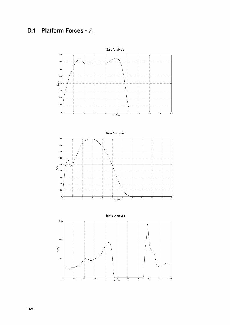
D.1 Platform Forces - Fz
D-2


![Competency Framework for Nursing Staff working within the ...1].… · 4 Competency Framework for Nursing Staff working within the Scottish Prison Service Competency Framework for](https://img.pdfslide.us/doc/110x75/5e209b28a41ada38270030d5/competency-framework-for-nursing-staff-working-within-the-1-4-competency.jpg)