Embed Size (px)
Citation preview

Development of a mathematical model for theoccupancy of mRNA with ribosomes in
Saccharomyces cerevisiae
Jannis UhlendorfBachelor Thesis
Freie Universitat BerlinDepartment of Mathematics and Computer Science
Bioinformatics Program
Advisors:Professor Dr. Edda Klipp
Professor Dr. Per Sunnerhagen
Max Planck Institute for Molecular GeneticsIhnestraße 63-73
14195 BerlinGermany
Email: [email protected]
June 6th - August 1st 2006


Abstract
This thesis describes the development of a mathematical model for the occupancy of mRNAwith ribosomes in the yeast Saccharomyces cerevisiae. The model is supposed to describethe change in polysomal association of mRNA, that is found when yeast cells are subjectedto a hyperosmotic shock. A hyperosmotic shock is a rapid increase of the osmolarity of thesurrounding media of a cell. Yeast cells respond with a variety of changes to hyperosmotic shock,including a down regulation of the translational apparatus. This means that the number ofribosomes an average mRNA has bound decreases. In this thesis different models to simulatethis behavior are developed, and tested for their properties and their ability to describe thetranslational downregulation after osmotic shock.
Inhalt
Diese Arbeit beschreibt die Entwicklung eines mathematischen Modells fur die Beladung vonmRNA mit Ribosomen in der Hefe Saccharomyces cerevisiae. Das Modell soll die Anderungder polysomalen Assoziierung von mRNA beschreiben, wenn Hefezellen einen hyperosmotischenSchock erfahren. Ein hyperosmotischer Schock ist eine schnelle Zunahme der Osmolaritat desumgebenden Mediums einer Zelle. Hefezellen reagieren mit einer Vielzahl von Anderungenauf einen hyperosmotischen Schock, unter Anderem mit einer Herabregelung der Translation.Dies bedeutet, daß die Zahl der Ribosomen, die eine durchschnittliche mRNA gebunden hatabnimmt. In dieser Arbeit werden verschiedene Modelle entwickelt um dieses Verhalten zubeschreiben und auf ihre Fahigkeit hin getestet, die osmotische Stressantwort von Hefezellenzu beschreiben.

Acknowledgements
First of all I would like to thank my supervisors Edda Klipp and Per Sunnerhagen for not onlymaking this work possible, but also for their great support and the many vital comments onmy work. In addition I would like to thank Malin Hult for her brilliant explanations that wereessential for this work. Thank you, Malin and Per for providing me with the data this work isbased on. Also, I would like to thank Axel Kowald, Jorg Schaber and Wolf Liebermeister for alot of ideas and comments on my work, and Katharina Albers, Matteo Barberis, and MarvinSchulz for carefully proof reading the manuscript.
3
Contents
Summary 2
Preface 3
1 Introduction 11.1 Objective . . . . . . . . . . . . . . . . . . . . . . . . . . . . . . . . . . . . . . . 11.2 Modeling biological processes . . . . . . . . . . . . . . . . . . . . . . . . . . . . 1
1.2.1 Mathematical description . . . . . . . . . . . . . . . . . . . . . . . . . . 21.3 Biological basis . . . . . . . . . . . . . . . . . . . . . . . . . . . . . . . . . . . . 3
1.3.1 Gene expression in eukaryotes . . . . . . . . . . . . . . . . . . . . . . . . 31.3.2 Osmoadaption in yeast . . . . . . . . . . . . . . . . . . . . . . . . . . . . 81.3.3 Sensing and signaling osmotic changes . . . . . . . . . . . . . . . . . . . 8
1.4 Methods . . . . . . . . . . . . . . . . . . . . . . . . . . . . . . . . . . . . . . . . 101.4.1 DNA Microarrays . . . . . . . . . . . . . . . . . . . . . . . . . . . . . . . 101.4.2 Analysis of polysomes . . . . . . . . . . . . . . . . . . . . . . . . . . . . 111.4.3 Gillespie algorithm for stochastic simulation . . . . . . . . . . . . . . . . 131.4.4 Differential Evolution algorithm for optimization . . . . . . . . . . . . . . 15
2 Model construction 172.1 Models . . . . . . . . . . . . . . . . . . . . . . . . . . . . . . . . . . . . . . . . . 17
2.1.1 Single rate model . . . . . . . . . . . . . . . . . . . . . . . . . . . . . . . 172.1.2 Multiple rate model . . . . . . . . . . . . . . . . . . . . . . . . . . . . . . 172.1.3 Bitstring model . . . . . . . . . . . . . . . . . . . . . . . . . . . . . . . . 182.1.4 mRNA degradation and production . . . . . . . . . . . . . . . . . . . . . 182.1.5 Degradation and production of ribosomes . . . . . . . . . . . . . . . . . . 19
3 Model analysis 203.1 Mathematical analysis . . . . . . . . . . . . . . . . . . . . . . . . . . . . . . . . 20
3.1.1 Single rate model . . . . . . . . . . . . . . . . . . . . . . . . . . . . . . . 203.1.2 Multiple rate model . . . . . . . . . . . . . . . . . . . . . . . . . . . . . . 223.1.3 Bitstring model . . . . . . . . . . . . . . . . . . . . . . . . . . . . . . . . 23
3.2 Simulation analysis . . . . . . . . . . . . . . . . . . . . . . . . . . . . . . . . . . 243.2.1 Single rate model . . . . . . . . . . . . . . . . . . . . . . . . . . . . . . . 253.2.2 Multiple rate model . . . . . . . . . . . . . . . . . . . . . . . . . . . . . . 263.2.3 Bitstring model . . . . . . . . . . . . . . . . . . . . . . . . . . . . . . . . 28
4

4 Data fit 314.1 Data . . . . . . . . . . . . . . . . . . . . . . . . . . . . . . . . . . . . . . . . . . 314.2 Used tools . . . . . . . . . . . . . . . . . . . . . . . . . . . . . . . . . . . . . . . 31
4.2.1 SBMLpet . . . . . . . . . . . . . . . . . . . . . . . . . . . . . . . . . . . 324.2.2 Berkeley Madonna . . . . . . . . . . . . . . . . . . . . . . . . . . . . . . 324.2.3 Matlab . . . . . . . . . . . . . . . . . . . . . . . . . . . . . . . . . . . . . 33
4.3 Steady state fit . . . . . . . . . . . . . . . . . . . . . . . . . . . . . . . . . . . . 344.3.1 Single rate model . . . . . . . . . . . . . . . . . . . . . . . . . . . . . . . 344.3.2 Multiple rate model . . . . . . . . . . . . . . . . . . . . . . . . . . . . . . 354.3.3 Bitstring model . . . . . . . . . . . . . . . . . . . . . . . . . . . . . . . . 37
4.4 Time course fit . . . . . . . . . . . . . . . . . . . . . . . . . . . . . . . . . . . . 404.4.1 Multiple rate model . . . . . . . . . . . . . . . . . . . . . . . . . . . . . . 404.4.2 Model with 3 initiation rates . . . . . . . . . . . . . . . . . . . . . . . . . 42
5 Results 475.1 Comparison . . . . . . . . . . . . . . . . . . . . . . . . . . . . . . . . . . . . . . 47
5.1.1 Models . . . . . . . . . . . . . . . . . . . . . . . . . . . . . . . . . . . . . 475.1.2 Processes . . . . . . . . . . . . . . . . . . . . . . . . . . . . . . . . . . . 48
5.2 Validation . . . . . . . . . . . . . . . . . . . . . . . . . . . . . . . . . . . . . . . 495.3 Conclusions . . . . . . . . . . . . . . . . . . . . . . . . . . . . . . . . . . . . . . 54
A Proofs 55A.1 Derivation of fomulae (3.5) and (3.6) . . . . . . . . . . . . . . . . . . . . . . . . 55A.2 Derivation of formula (3.7) . . . . . . . . . . . . . . . . . . . . . . . . . . . . . . 56
B Deterministic simulation in MATLAB 58
Bibliography 61
5

Abbreviations
Abbrevation Meaning or ContextBM Berkeley MadonnaCdc24 HOG PathwayCdc42 HOG PathwayCPSF Cleavage and Polyadenylation Factor (Transcription Termination Factor)CstF Cleavage Stimulation Factor F (Transcription Termination Factor)eEF-1A Translation Elongation FactoreEF-2 Translation Elongation FactoreIF-2 Translation Initiation FactoreIF-2B Translation Initiation FactoreIF-4A Translation Initiation FactoreIF-4E Translation Initiation FactoreIF-4G Translation Initiation FactorER Endoplasmatic ReticulumeRF-1 Translation Release FactoreRF-3 Translation Release FactorFps1p Glycerol ChannelDE Differential EvolutionHOG High Osmolarity GlycerolHog1 HOG PathwayMAP Mitogen Activated ProteinMAP-KK MAP Kinase KinaseMAP-KKK MAP Kinase Kinase KinaseMCA Metabolic Control AnalysismiRNA Micro RNAmRNA Messenger RNAODE Ordinary Differential EquationPAF Polysomal Association FactorPbs2 HOG Pathwaypre-mRNA Premature Messenger RNArRNA Ribosomal RNARSSQ Residual Sum Of SquaresSBML Systems Biology Markup LanguageSho1 HOG PathwaySln1 HOG PathwaysnoRNA Small Nucleolar RNAsnRNA Small Nuclear RNASsk1 HOG PathwaySsk2 HOG PathwaySsk22 HOG PathwaySte11 HOG PathwaySte20 HOG PathwaySte50 HOG PathwayTFIIA Transcription Initiation FactorTFIIB Transcription Initiation FactorTFIID Transcription Initiation FactorTFIIE Transcription Initiation FactorTFIIF Transcription Initiation FactorTFIIH Transcription Initiation FactortRNA Transfer RNAUTR Untranslated RegionUV UltravioletYpd1 HOG Pathway
6
List of Tables
3.1 Parameters for simulation 3.5 . . . . . . . . . . . . . . . . . . . . . . . . . . . . 28
4.1 Parameters for steady state fit - single rate model . . . . . . . . . . . . . . . . . 354.2 Parameters for steady state fit - multiple rate model . . . . . . . . . . . . . . . . 384.3 Parameters for steady state fit - bitstring model . . . . . . . . . . . . . . . . . . 394.4 Parameter k transcr for time course fit - multiple rate mRNA production A . . 414.5 Parameters for time course fit - multiple rate ribosome degradation A . . . . . . 424.6 Parameters for time course fit - multiple rate model initiation rate change . . . . 444.7 Parameters for time course fit - multiple rate model mRNA production B . . . . 454.8 Parameters for time course fit - multiple rate model ribosome degradation B . . 46
7

List of Figures
1.1 Gene expression in eukaryotes . . . . . . . . . . . . . . . . . . . . . . . . . . . . 41.2 Map of the HOG pathway . . . . . . . . . . . . . . . . . . . . . . . . . . . . . . 91.3 Example of polysomal profile . . . . . . . . . . . . . . . . . . . . . . . . . . . . . 121.4 Different methods for polysomal profiling . . . . . . . . . . . . . . . . . . . . . . 13
3.1 Single rate model: Plot of X against mRNA concentrations . . . . . . . . . . . . 213.2 Single rate model: Simulation of ribosome degradation . . . . . . . . . . . . . . 223.3 Simulation of single rate model . . . . . . . . . . . . . . . . . . . . . . . . . . . 253.4 Multiple rate model Simulation A . . . . . . . . . . . . . . . . . . . . . . . . . . 263.5 Multiple rate model Simulation B . . . . . . . . . . . . . . . . . . . . . . . . . . 273.6 Multiple rate model polysome distribution . . . . . . . . . . . . . . . . . . . . . 283.7 Bitstring model simulation A . . . . . . . . . . . . . . . . . . . . . . . . . . . . 293.8 Bitstring model simulation B . . . . . . . . . . . . . . . . . . . . . . . . . . . . 30
4.1 Example of polysomal profile . . . . . . . . . . . . . . . . . . . . . . . . . . . . . 324.2 Goodness of fit Berkeley Madonna . . . . . . . . . . . . . . . . . . . . . . . . . . 334.3 Goodness of fit - single rate model time point 0 . . . . . . . . . . . . . . . . . . 364.4 Goodness of fit - single rate model time point 10 . . . . . . . . . . . . . . . . . . 374.5 Goodness of fit - bitstring model time point 0 . . . . . . . . . . . . . . . . . . . 394.6 Goodness of time course fit - multiple rate model mRNA production A . . . . . 414.7 Goodness of time course fit - multiple rate model ribosome degradation A . . . . 434.8 Goodness of time course fit - multiple rate model initiation rate change . . . . . 444.9 Goodness of time course fit - multiple rate model mRNA production B . . . . . 454.10 Goodness of time course fit - multiple rate model ribosome degradation B . . . . 46
5.1 Change in the polysomal association factor after osmotic shock for different typesof genes . . . . . . . . . . . . . . . . . . . . . . . . . . . . . . . . . . . . . . . . 50
5.2 PAF simulation for bistring model . . . . . . . . . . . . . . . . . . . . . . . . . . 515.3 Simulation bitstring model upregulated mRNA . . . . . . . . . . . . . . . . . . . 525.4 Simulation bitstring model downregulated mRNA . . . . . . . . . . . . . . . . . 535.5 Simulation bitstring model not regulated mRNA . . . . . . . . . . . . . . . . . . 53
B.1 MATLAB code for gradient function . . . . . . . . . . . . . . . . . . . . . . . . 59B.2 MATLAB code for simulation . . . . . . . . . . . . . . . . . . . . . . . . . . . . 60
8
Chapter 1
Introduction
1.1 Objective
The aim of this work has been to develop a mathematical model, that explains the change in
the polysomal association of mRNAs in Saccharomyces cerevisiae when subjected to osmotic
stress. Yeast cells that are transfered to a medium of high osmolarity show a specific response
(Hohmann, 2002), which includes the global downregulation of the translational apparatus.
This means that the polysomal profile of the cells, is shifted from a distribution consisting of
highly translated mRNAs (polysomes) to a distribution formed by lower translated mRNAs.
In this work different models for the occupancy of mRNA with ribosomes have been devel-
oped and tested for their ability to describe both, the distribution of polysomes in unstressed
cells, and the temporal change in the polysomal pattern after osmotic shock. For this purpose
different processes that may cause the change in the translation state in response to osmotic
shock have been incorporated in the different model, and examined for their influence on these
models.
1.2 Modeling biological processes
Systems Biology attempts to understand the biology at system level (Kitano, 2002). This means
understanding the system in general, rather than focusing on isolated subsystems. Because of
the complexity of living organisms, which dooms unstructured attempts to globally understand
them to fail, this approach can only be successful by making use of a general mathematical
description of the underlying processes. Methods for the global mathematical analysis of reac-
tion systems have been developed, for instance the metabolic control analysis (MCA) allows to
determine the influence of single reactions or metabolites on the whole reaction system (Kacser
and Burns, 1973; Heinrich and Rapoport, 1974). For the mathematical description of reaction
systems a general approach exists, which shall be described in the following section.
1

1.2.1 Mathematical description
The mathematical description of a reaction system can be formulated in a general way (Klipp
et al., 2005a). First of all, the topology of the network can be described by the stoichiometric
matrix. The stoichiometric matrix N consists of a column for each reaction and a row for each
substrate. The element nij is the stoichiometry at which the ith substrate participates in the
jth reacion, or 0 if the substrate does not take part in this reaction. The simple reaction system
r1→ S0r2→ S1
r3→
leads to the stoichiometric matrix
N =
(1 −1 00 1 −1
)
The concentration change of a metabolite in time is the sum of the concentration changes
that are caused by the particular reactions, in which the metabolite participates. Therefore, the
concentration change of a metabolite is given by its row in the stoichimetric matrix multiplied
with the vector of reaction velocities v. This can be written in as:
dSidt
=
r∑
j=1
nij · vj (1.1)
where vj denotes the reaction velocity of the jth reaction.
The substrate concentrations also can be collected in a vector S, where si denotes the con-
centration of substrate i. The reaction velocity vector v generally depends on the concentration
of all metabolites S and the parameters p, which can be written as v = v(S, p).
Equation (1.1) can be written in matrix notation as:
dS
dt= Nv = Nv(S, p) (1.2)
To investigate the properties of such a model, it is generally considered to be in steady state,
which means that none of the substrate concentrations changes over time. A concentration
change for one of the metabolites would mean that this substrate is either removed from the
system, or accumulated. This cannot be if the system is balanced. The steady state assumption
can be written in mathematical terms as:
dS
dt= Nv = 0 (1.3)
Solving this equation for the reaction velocities v gives the fluxes J that can be reached in steady
state. The fluxes J differ from the reaction velocities, in the point that they only depend on
the parameters p, not on the concentrations S.
J(p) = v(S, p) (1.4)
2
Solving Equation (1.3) for the metabolite concentrations gives the metabolite concentrations
S(p) that can be reached in a steady state, in dependence of the parameters p. Unfortunately,
in most of the cases it is not possible to solve Equation (1.3) analytically.
Equation (1.2) gives a deterministic description of the reaction system, which means that
for known initial concentrations S and parameters p, the concentrations can be determined
for every proximate time point by integrating this equation over the time. This can be done
analytically to get a general mathematical description, if the system is not too complicated, or
numerically to simulate the system.
The deterministic approach requires that (i) the system is well mixed, and (ii) the molecule
numbers are high. For small molecule numbers also stochastic processes play a role, since
molecule numbers can only adopt discrete values. A stochastic description of a reaction system
gives the probability for each possible way in which the system can evolve. A way in this
context is made up by the concentrations of all metabolites at all time points. A stochastic
simulation chooses one possible way in which the system could evolve, but does this according
to the probability that the system will evolve in this direction.
1.3 Biological basis
1.3.1 Gene expression in eukaryotes
Gene expression denotes the process of converting information, that is contained in the DNA
sequence of a gene, into structural or signaling elements of the cell. These elements are proteins
in most cases, but can also be RNAs. In Saccharomyces cerevisiae, for example, more than
700 of its roughly 6000 genes produce RNA as their final product (Eddy, 1999; Goffeau et al.,
1996). When we speak of RNA, we usually mean the messenger RNA (mRNA) that serves
as a template for protein synthesis. But there exist also a variety of other RNA types in the
cell, which are termed after their function. The most important noncoding RNAs are ribosomal
RNAs (rRNA), which are an essential part of the ribosome, transfer RNAs (tRNA), which serve
as adaptors beween the mRNA and amino acids during translation, microRNAs (miRNA)
which are thought to regulate the expression of other genes, small nuclear RNAs (snRNA),
which among other things play an important role during splicing, and small nucleolar RNAs
(snoRNA), which process rRNAs. In eukaryotes, the different types of mRNA are produced by
three different RNA-polymerases.
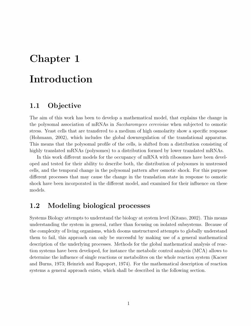
The process of gene expression for protein coding RNAs is displayed in Figure 1.1. In the
first step, a region on the DNA called transcription unit is transcribed to a complementary RNA.
The catalyzing enzyme is the RNA-polymerase II, and the RNA product is called premature
messenger RNA (pre-mRNA). This pre-mRNA undergoes several modifications, before it is
engaged in protein synthesis (Lewis and Tollervey, 2000). The first modification is the addition
of a modified guanine nucleotide at the 5’ end, which already takes place during transcription.
This cap is important for the binding of ribosomes to the designated mRNA. On the other end
of the pre-mRNA a set of adenosine residues is added, forming a so called polyA tail, which
3
determines the stability of the mRNA and serves as an export signal from the nucleus (Huang
and Carmichael, 1996; Drummond et al., 1985). The third modification is called splicing
and denotes a process in which noncoding regions of the mRNA are excised. This process is
catalyzed by a RNA-protein complex called splicosome, which cuts out the noncoding regions
(introns) in a two step process. By varying the number and positions of splice events, a process
called alternative splicing, it is possible also for a eucaryotic cell to encode different proteins
on a single gene (Black, 2000). Another optional modification is the change of the nucleotide
composition of the mRNA, called RNA editing.
Figure 1.1: Gene expression in eukaryotes
After the pre-mRNA has undergone the above described post transcriptional modifications,
it is a mature mRNA and ready to be exported to the cytosol. This export is highly selective to
ensure that only correct processed mRNAs are translated. The nuclear pore complex recognizes
several indications for the processing state of an mRNA, and exports only mature mRNAs
(Daneholt, 1997). In the cytosol ribosomes bind to the 5’ cap of the mRNA and translate
its base sequence into the amino acid sequence of a protein. The synthesis of all proteins
takes place in the cytosol. Proteins that contain a special signal sequence are recruited to the
endoplasmatic reticulum (ER) during translation, where the ribosome synthesizes the protein
directly into the ER lumen. In the ER proteins are further processed by the addition and
trimming of oligosaccharides before they are passed on to the golgi apparatus, which is also
involved in the oligosaccharide processing, and finally sorts and packages the proteins for further
transport.
It is important to mention that the above described processes correspond to eukaryotic
cells. In bacteria the processes are somewhat easier, although they are similar. Fundamental
differences are the absence of post transcriptional modifications, the use of just one RNA
polymerase, and the potential to encode more than one protein on one mRNA in procaryotes.
For further details on the described biological processes see (Alberts et al., 2002).
Since the cell has to be able to control its protein synthesis, another fate of the cytoplasmic
mRNAs is the degradation by ribonucleases. The degradation rate of different mRNAs depends
4
on the type of the mRNA (Lowell et al., 1992) as well as on the environmental and intrinsic
conditions of the cell (Bernstein and Ross, 1989; Zingg et al., 1988).
Cells have to be able to alter their gene expression because of specialization in a multicel-
lular organism, and in response to environmental changes. These differences in mRNA and
protein levels occur not due to changes in the DNA sequence, but are controlled by a variety
of mechanisms that intervene in processes during or downstream to transcription (Gurdon,
1968). The regulation of gene expression can be roughly divided into transcriptional and post
transcriptional control mechanisms.
Transcriptional control mechanisms
The transcription is classified into the three steps: initiation, elongation, and termination. Each
of these steps requires not only the RNA polymerase, but a large number of helping proteins
named transcription factors.
Initiation starts with the binding of the general transcription factor TFIID to a region,
typically located 25 nucleotides upstream from the transcription start, called TATA box. The
binding of TFIID causes the binding of several other transcription factors (TFIIA, TFIIB,
TFIIE, TFIIF, and TFIIH) as well as the RNA polymerase II (Conaway and Conaway, 1993).
TFIIH plays an important role in unwinding the RNA and in the activation the polymerase
by phosphorylation. Altogether, well over 100 subunits are involved in transcription initiation.
To assemble this huge machinery a mediator protein complex is required. This mediator binds
to a specific DNA sequence, thereby activating the transcription for a specific gene.
After the initiation most of the initiation factors dissociate, and elongation factors bind to
the polymerase. These elongation factors reduce the probability of dissociation of the poly-
merase from the RNA. Likewise are termination factors required, that recognize the polyadeny-
lation site in the growing RNA, thereby terminating the elongation process. The termination
factors cleavage stimulation factor F (CstF) and cleavage and polyadenylation factor (CPSF)
recognize the termination signal in the growing RNA sequence, and as their name indicates
trigger the cleavage of the mRNA chain and the addition of a poly-A tail, which is catalyzed
by the poly-A polymerase. The poly-A tail is bound by poly-A binding proteins.
Regulation of transcription is possible at various of the described steps. First of all, the ini-
tiation of transcription often requires the remodeling of the chromatin structure of the DNA to
facilitate binding of the polymerase to the DNA. This task is fulfilled by chromatin remodeling
complexes, which can be selectively brought to specific regions of the DNA, thereby activating
specific genes (Kingston, 1999). Other gene regulatory proteins bind to specific DNA sites,
thereby either activating genes by attracting general transcription factors or the polymerase to
the DNA region (enhancers), or inhibiting the formation of the initiation complex (repressors)
(Kornberg, 1999). Besides the regulation of initiation, there exist also proteins that regulate
the rate of elongation (Bentley, 1995). A mechanism that is only present in vertebrates is
the methylation of DNA regions, which leads to the binding of proteins, which remodel the
chromatin structure, making the DNA transcriptionally inactive.
5

Of course most gene regulatory proteins do not act on their own, but are then again regulated
upstream signaling pathways.
Post transcriptional control mechanisms
Post transcriptional control includes all the gene regulatory processes that occur after tran-
scription. One way of post transcriptional control is the above mentioned alternative splicing
process, where certain splice sites are left out, or cryptic splice sites are activated. This alter-
native splicing does not exclusively occur by chance, but is also regulated by other molecules
in both positive and negative way.
As also noted above, the coding sequence of mRNA can be changed by enzymes after
transcription in a process called RNA editing.
Another way to regulate the translation rate of mRNAs is the control of export from the
nucleus, since protein synthesis only takes place in the cytosol. To be exported, an mRNA
needs to be correctly capped, polyadenylated, and spliced. This mechanism is known to play a
role in stress induced differential gene expression (Saavedra et al., 1996).
Furthermore, the distribution of mRNAs over the cytoplasm is not random, but a regulated
process (Ding and Lipshitz, 1993; Singer, 1992; Wilhelm and Vale, 1993). This is an economic
way of the cell to direct proteins to their destination, as it only requires the transport of the
mRNA instead the produced proteins. The signals directing the mRNA localization are usually
found in the 3’-UTR of the mRNA.
The translation of mRNAs is also controlled by the cell. Several proteins for example bind
to the 5’ end of the mRNA, thereby inhibiting the translation initiation. Other proteins bind
to the 3’ poly-A tail and disturb the communication between the 5’ cap and the 3’ poly-A tail,
which is required for efficient translation. Global regulation of the protein synthesis rate can
be achieved by the phosphorylation of the initiation factor eIF-2 (Wek, 1994), which normally
mediates the binding of the methionyl-tRNA to the 40S ribosomal subunit. Phosphorylation
of eIF-2 enhances its affinity to eIF-2B, which is required for eIF-2 to release its bound GDP
after the initiation process. This leads to the consumption of eIF-2B, thereby arresting the
reactivation of eIF-2 which again induces a lower initiation rate.
A very important way for the cell to regulate the expression of certain genes is the degrada-
tion rate of the corresponding mRNAs. It has been shown that the half-lives of mRNAs vary
from less than one minute to more than one hour (Herrick et al., 1990; Jacobson et al., 1990),
what indicates a contribution of this mechanism to differential gene expression. The polyA tail
plays an important role in this pathway (Wilson et al., 1978). In the cytosol the polyA tail
is shortened continuously by exonucleases, and once the length of the polyA tail falls below a
threshold a degradation pathway is triggered. This degradation pathway involves the removal
of the 5’ cap in a process called decapping and the subsequent degradation of the mRNA.
The proteins that shorten the polyA tail compete in general with the translational apparatus,
wherefore a well translated mRNA is subjected to a lower degradation than a less translated
one (Prieto et al., 2000). The degradation of the polyA tail is also thought to be influenced
6
by proteins, that bind to specific sequences in the 5’ UTR. There exist a second pathway for
mRNA degradation in which an exonuclease cleaves away the polyA tail, which lead again to
degradation of the mRNA. mRNAs which are degraded in this way carry a special signal in
their 5’ UTR. For a comprehensive review on post transcriptional control see (McCarthy, 1998).
Translation
The translation is the process of decoding the nucleotide sequence of an mRNA into a protein’s
primary structure. The location of translation is the cytoplasm, so the mRNA has to be
exported from the nucleus in advance. The initiation of translation begins with the binding of
the initiator tRNA, which carries methionine, to the small ribosomal subunit. This requires
also the binding of the eucaryotic initiation factor eIF-2. After that the small ribosomal subunit
binds to the 5’ cap of the mRNA, whereby the selective binding of the cap is achieved by the
initiation factor eIF-4E. For the binding of the 40S ribosomal subunit and eIF-4E also eIF-G
is required, which is supposed to mediate the binding of the ribosomal subunit and to enhance
the cap binding of eIF-4E (Ptushkina et al., 1998). After the binding to the cap, the complex,
consisting of the 40S subunit and the initiation factors, moves along the 5’ untranslated region
(5’ UTR) until it encounters an AUG start codon. This searching may be driven by the initiation
factor eIF-4A (Sonenberg, 1996). Once the complex has found an AUG codon, the initiation
factors dissociate and the big 60S ribosomal subunits binds to form the complete 80S ribosome.
The nucleotides surrounding the AUG codon influence the efficiency of the AUG recognition,
thereby providing a mechanism to code more than one protein even on a eukaryotic mRNA.
The ribosome has three binding sites for tRNAs, the aminiacyl-tRNA-site (A), the peptidyl-
tRNA-site (P), and the exit-site (E). After the formation of the ribosome, the methionine-tRNA
is bound to the P-site. During elongation the tRNA that matches the next codon binds to the
A-site, allowing the ribosome to catalyze a peptide bond between its bound amino acid and the
growing peptide chain. During this reaction the new tRNA moves from the A-site to the P-site,
while the preceding tRNA moves to the E-site, where it is released. At this time the tRNA is
located in the P-site, and holds the growing peptide chain covalently linked, while the A-site is
vacant and can be accessed by the next tRNA. As for the initiation various elongation factors
are required for the elongation process. eEF-1A forms a complex with GTP and aminoacyl-
tRNA, facilitating the binding to the ribosome. eEF-2 helps in translocating the peptidyl-tRNA
to the P site, and is likely to be regulated in higher cells (Pain, 1996; Nairn and Palfrey, 1996)
Termination of the translation process is induced by the occurrence of one of the stop codons
(UAA, UAG, or UGA), which have no matching tRNAs, but instead trigger the binding of the
release factors eRF-1 and eRF-3 to the A-site. The release factors initiate the release of the
peptide chain by the addition of water, and the disaggregation of the ribosome.
Because the translation of an average mRNA takes longer than it takes for the next initiation
process to take place, mRNAs are not only transcribed by a single ribosome, but instead form
a complex with several ribosomes called polyribosomes (or polysomes).
7

1.3.2 Osmoadaption in yeast
The osmolarity of the surrounding media is very important for a cell, since it determines its
turgor pressure. Osmolarity is a measurement for the amount of solutes per litre of solution.
Because the interior of a cell has generally a higher osmolarity than the surrounding medium,
there is a constant force driving water into the cell to offset this imbalance. This force leads to
an antagonizing force arising from the limited expansion ability of the plasma membrane and
the cell wall, which is called turgor pressure (Blomberg and Adler, 1992; Wood, 1999).
Since the osmolarity of the medium surrounding the cell can change, a cell has to be able to
respond to those changes in order not to shrink or to burst. When cells are subjected to a so
called hyperosmotic shock, which is a rapid upshift of the extracellular osmolarity, they have
to deal with water outflow and consequent cell shrinkage. On the other hand, a hypoosmotic
shock (osmotic downshift) leads to water influx and thereby to increased turgor pressure. The
cell senses osmotic changes by certain receptors, and relays them through different signaling
pathways to alter gene expression and the production and transport of certain metabolites. A
mathematical model for the osmotic stress response of yeast is available (Klipp et al., 2005b),
but this model does not include the occupancy of mRNA with ribosomes. A very comprehensive
review about the signaling and response of yeasts to osmotic stress has been written by Stefan
Hohmann (Hohmann, 2002).
1.3.3 Sensing and signaling osmotic changes
There exist several proteins sensing osmotic changes. They either act similar to chemosensors,
with the difference that they are not restricted to a certain compound, or sense mechanical
changes that result from the osmotic shift. In Saccharomyces cerevisiae the Sln1 and Sho1
proteins are the most prominent osmotic sensors, both controlling the high osmolarity glycerol
(HOG) pathway (see Figure 1.2).
The Sln1 pathway is active under low osmolarity conditions, where it acts by inhibiting the
HOG pathway. The signal transduction from Sln1 to HOG1 can be divided in two modules, a
two component phosphorelay module, and a mitogen activated protein (MAP) kinase module.
The two component module is actually a three component system comprising the proteins Sln1,
Ypd1 and Ssk1. The two component in the name indicates the similarity of the module to
classical procaryotic two-component transduction systems (Widmann et al., 1999). Sln1 has an
autophosphorylytic activity, which is active under normal osmotic conditions, and is inhibited
by high osmolarity. The autophosphorylation of Sln1 implicates the phosphorylation of Ypd1,
which again transfers the phosphate group to Ssk1. Ssk1 stimulates the downstream MAP
kinase module by the phosphorylation of Ssk2 and Ssk22, but is inactivated by phosphorylation.
Thereby, high osmolarity activates the pathway by dephosphorylation of Ssk1.
The following MAP kinase module consists of the four components: Ssk2, Ssk22 (both MAP
kinase kinase kinase (MAP-KKK)), Pbs2 (MAP kinase kinase (MAP-KK)), and Hog1 (MAP
kinase). Hog1 then again activates several factors that are important for the stress response.
MAP kinase signaling cascades generally consist of three proteins, that amplify an incoming
8

Figure 1.2: Map of the HOG pathway
signal by passing on phosphorylation signals. A simple three component MAP kinase cascade
would consist of an MAP-KKK element, which is activated by an activator (e.g a receptor) and
thereupon phosphorylates the MAP-KK. In the phosphorylated state MAP-KK activates the
protein MAP-kinase (by phosphorylation), which activates certain effector proteins affecting
their activity.
In addition to the Sln1 pathway, yeast cells activate the MAP kinase module by another
osmotic sensor, the Sho1 pathway (Helliwell et al., 1994). Sho1 is active under high osmolarity
conditions and activates the G-Protein Cdc42, which relays the signal to kinase Ste20, that again
activates the MAP-KKK Ste11. This reaction sequence also requires Cdc24, the exchange factor
for Cdc42, and Ste50 (Raitt et al., 2000). Ste20 is a MAP-KKK and activates the MAP-KK
Pbs2 in the MAP kinase module, thereby converging the two pathways.
Response to osmotic changes
When the cell is subjected to a rapid osmotic upshift, it shrinks within seconds to a fraction of
its initial volume (Albertyn et al., 1994).
Consequences of osmotic upshift include an enhanced production of glycerol and trehalose,
and the reduction of glycerol export. Glycerol is a very important osmoactive substance in
the cell, and increased cellular concentration of glycerol can countervail the increased external
osmolarity. The glycerol metabolism is effected quite dramatically by hyperosmotic shock, as
the genes for glycerol synthesis (GPD1 and GPP2) transiently increase up to about 50-fold
9

(Albertyn et al., 1994; Hirayarna et al., 1995; Norbeck et al., 1996). In addition, Fps1p, a cell
wall channel for glycerol, is regulated negatively in response to hyperosmotic shock (Tamas
et al., 1999; Luyten et al., 1995).
General pathways of the cell such as amino acid metabolism, cell wall maintenance, nucleo-
some structuring, DNA synthesis, and nucleotide metabolism are downregulated under osmotic
stress (Hohmann, 2002). In addition, the elongation step of protein synthesis is also believed
to be downregulated by osmotic stress (Teige et al., 2001).
Also the production of trehalose and glycogen is found to increase in response to (not
exclusively) osmotic stress (Causton et al., 2001; Gasch et al., 2000). Trehalose is a disaccharide
which is important for cells to survive under stress (Deschenes et al., 1999; Estruch, 2000;
Francois and Parrou, 2001; Nwaka et al., 1995; Singer and Lindquist, 1998), and glycogen is a
polysaccharide which serves as a energy storage in the cell. However, the increased production
of trehalose does not accumulate it in the cell (Hounsa et al., 1998), which is due to likewise
increased degradation.
1.4 Methods
1.4.1 DNA Microarrays
DNA microarrays provide a method to monitor the complete expression pattern of a cell in a
single experiment (Southern, 2001). An array consists of a huge number of small DNA pieces
that are each complementary to a certain gene (or rather transcript). When this DNA chip
is incorporated with stained RNA or DNA, the probes bind to the spot on the array which is
their complement. As the positions of each gene is known on a microarray, this enables the
experimentalist to quantify the abundance of each gene transcript by analyzing the intensity
of the stains. In practice two variants of microarrays are commonly used:
cDNA Arrays
cDNA arrays consist of pieces of DNA, that are complementary to the genes of interest (e.g. all
6000 yeast genes). They measure the relative RNA abundance of two probes and are therefore
also referred to as two channel arrays. In an experiment the RNA of two cell types (e.g stressed
and unstressed cells) is reverse transcribed to cDNA, which is labeled with a flurescent dye. In
this step it is important to label the two different probes with two distinct dyes. Commonly,
one probe is labeled with the green-flurescending Cy3, while the other probe is labeled with the
red-flurescending dye Cy5. Hybridizing the mixture of the two probes with the array results in
a competition of the two differently labeled probes for binding to the array. Therefore, a green
spot on the array indicates higher transcript level in the first probe, while a red spot indicates
the opposite. Consequently a yellow spot indicates a similar transcript level.
10

Oligonucleotide Arrays
Oligonucleotide arrays contain small oligonucleotide (≤ 25 base) strands, rather than larger
copies as in the cDNA arrays. In general 11 to 16 copies of each gene are included in the array,
which makes this type of array more specific, but less suitable for global analysis of whole
genomes. Another difference to the cDNA arrays is, that only one probe is analyzed in one
experiment, instead of comparing two expression patterns. The technical difference is that the
cDNA derived from the cellular RNA, is again transcribed to cRNA, which then is hybridized
to the array.
1.4.2 Analysis of polysomes
The activity at which mRNAs are translated is regulated both globally and specifically (Jo-
hannes et al., 1999; Zong et al., 1999; Kuhn et al., 2001; Mikulits et al., 2000; Brown et al.,
2001). The underlying mechanisms are described in section 1.3.1. The translation state can be
measured globally and for specific mRNAs. The methods how this is done are described in this
section.
Global polysomal profiling
A method to determine the global translation state of a cell is to separate the differently loaded
mRNAs by centrifugation, and to measure the abundance of RNA along this segregation by
absorbance of ultraviolet (UV) light. RNA absorbs light with at a wavelength of 254 nm, and
the absorbance of a solution containing RNA is proportional to the containing amount of RNA.
More precisely, the absorption at a certain wave length A is the concentration C multiplied
with way the light has to go through the solution I and an extinction coefficient ε (A = εCI).
This method has been used for example in (Swaminathan et al., 2006; Ashe et al., 2000;
Dickson, 1998). In the first step the cellular RNA, which is still being translated by ribosomes
is extracted and separated by high speed sedimentation centrifugation. This method separates
by density, thus the higher translated mRNAs are driven to the bottom of the centrifugation
tube. In the next step fractions are collected from the separated solution by isotonic pumping,
and changing the collecting bin at certain time intervals. These fractions contain the same
mRNA with different numbers of bound ribosomes and can be used for the specific analysis
described in the next paragraph. A global profile of the translation state of the cell can be
gained by monitoring the absorbance at wavelength 254 nm during the isotonic pumping.
Figure 1.3 shows an example of how such a measurement of the absorbance looks like. The
isotonic pumping starts from the top of the centrifuged solution, wherefore the highly translated
mRNA pertains to the right side of the graph. The high absorbance at the beginning of the
pumping is due to the absorbance of other solutes than RNA. After that, the graph shows
peaks for the big and small ribosomal subunit, and thereupon a big peak for the mRNAs
that are translated by one ribosome (monosomes). Behind the monosomes follow the different
polysomes. Since the polysomes consisting of more than 10 ribosomes can not be distinguished
11

in this analysis, they are pooled together. Furthermore this method gives no estimation for the
amount of mRNA that is not engaged in translation.
Figure 1.3: Example for a measurement of the global polysomal profile. Cellular RNA withthe associated ribosomes has been separated by gradient centrifugation. The gradient has beenmonitored for it’s RNA content by measuring the UV absorbance.
Specific polysomal profiling
In addition to the global analysis of the translation state, it is also possible to monitor the
change in translation for single mRNAs. Two methods are available here, the first determines
the abundance of certain mRNAs by northern blotting, and the second by DNA microarrays.
For the northern blotting method the RNA from the fractions collected during the isotonic
pumping (typically up to 15) are run separately on agarose gels and probed by northern blotting.
This gives a measurement for the abundance of individual mRNAs in the fractions. An idea how
this looks like can be obtained from Figure 1.4 B, although in this case the shown procedure is
not a northern blot but a simple RNA separation and subsequent staining. This method has
been applied for example in (Kuhn et al., 2001; Swaminathan et al., 2006; Arava et al., 2003).
The second type of analysis is to use DNA microarrays to quantify the abundance of a
huge number of mRNAs from one or more polysomal fractions. In general, a pool of polysomal
fractions is compared to total mRNA by the use of two channel arrays. This gives an estimate
of the translational activity of each single mRNA. This method has been applied in (Serikawa
et al., 2003; Swaminathan et al., 2006; Mata et al., 2005). It can be extended by comparing
multiple polysomal fractions to the total mRNA (MacKay et al., 2004). This approach is
illustrated in Figure 1.4 C.
12

Figure 1.4: (A) Absorbance profile as already shown in figure 1.3. (B) Separating the RNAfrom each fraction by electrophoresis shows the different types of RNA in each fraction. (C)A specific polysomal profile for single mRNAs can be achieved by comparing the fractionatedmRNA with the total mRNA on a microarray. Therefore the RNA from the fractions is reversetranscribed and labeled with Cy3, while the unfractionated RNA is reverse transcribed andlabeled with Cy3. Figure taken from (Arava et al., 2003)
1.4.3 Gillespie algorithm for stochastic simulation
The Gillespie algorithm (Gillespie, 1977) is a method to simulate a chemical reaction system
stochastically, which means that the algorithm chooses one possible way of the system, but
does this according to the probability that the system would evolve in this way. A way is here
defined as the number of all molecule numbers at each time point. When we consider a system
of N metabolites with molecule numbers X1, ..., XN at time point t that interact through M
reactions, Gillespie’s algorithm creates a time point t+ τ at which the next reaction will occur,
and states which reaction Rµ it will be. The important point is that the algorithm chooses
these values according to the reaction probability density function of the system. The reaction
probability density function P (τ, µ)dτ is the probability that, given the state (X1, ..., XN), the
next reaction will occur in the infinitesimal time interval (τ, τ+dτ) and that it will be Rµ. This
probability is the product of the probability that no reaction will happen in the interval (0, τ)
times the probability that reaction Rµ will occur in the interval (τ, τ + dτ). The probability
that there will be no reaction in the interval (0, τ) is
P0(τ) = e−PMv=1 avτ (1.5)
13
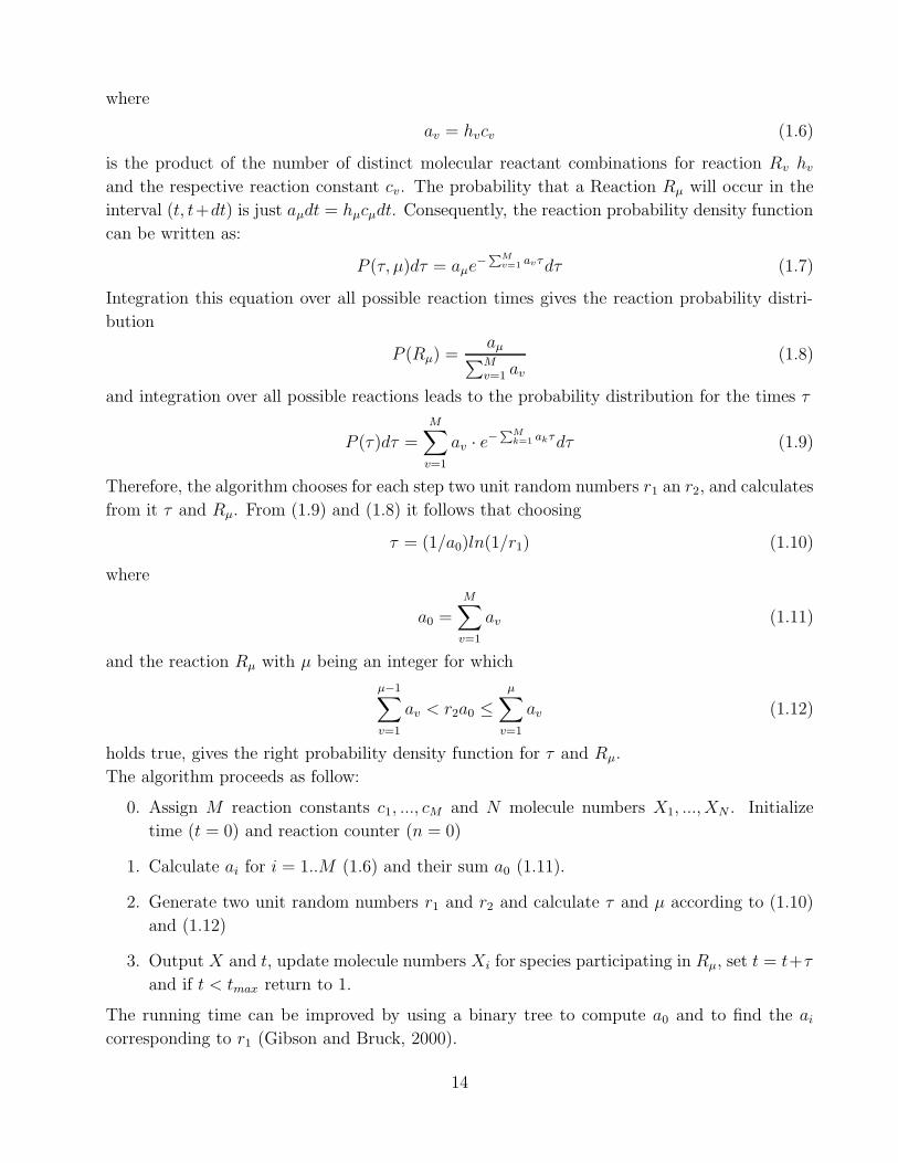
where
av = hvcv (1.6)
is the product of the number of distinct molecular reactant combinations for reaction Rv hvand the respective reaction constant cv. The probability that a Reaction Rµ will occur in the
interval (t, t+dt) is just aµdt = hµcµdt. Consequently, the reaction probability density function
can be written as:
P (τ, µ)dτ = aµe−PM
v=1 avτdτ (1.7)
Integration this equation over all possible reaction times gives the reaction probability distri-
bution
P (Rµ) =aµ∑Mv=1 av
(1.8)
and integration over all possible reactions leads to the probability distribution for the times τ
P (τ)dτ =
M∑
v=1
av · e−PMk=1 akτdτ (1.9)
Therefore, the algorithm chooses for each step two unit random numbers r1 an r2, and calculates
from it τ and Rµ. From (1.9) and (1.8) it follows that choosing
τ = (1/a0)ln(1/r1) (1.10)
where
a0 =
M∑
v=1
av (1.11)
and the reaction Rµ with µ being an integer for which
µ−1∑
v=1
av < r2a0 ≤µ∑
v=1
av (1.12)
holds true, gives the right probability density function for τ and Rµ.
The algorithm proceeds as follow:
0. Assign M reaction constants c1, ..., cM and N molecule numbers X1, ..., XN . Initialize
time (t = 0) and reaction counter (n = 0)
1. Calculate ai for i = 1..M (1.6) and their sum a0 (1.11).
2. Generate two unit random numbers r1 and r2 and calculate τ and µ according to (1.10)
and (1.12)
3. Output X and t, update molecule numbers Xi for species participating in Rµ, set t = t+τ
and if t < tmax return to 1.
The running time can be improved by using a binary tree to compute a0 and to find the aicorresponding to r1 (Gibson and Bruck, 2000).
14

1.4.4 Differential Evolution algorithm for optimization
Differential evolution (DE) (Storn and Price, 1997) is a heuristic to find the minimizing pa-
rameters for an arbitrary input function. The algorithm operates stochastically as the starting
parameters are chosen randomly, and the search for the best parameter also involves throw-
ing dices. The strategy is similar to the natural selection theory, wherefore DE borrows its
terminology.
The aim is to minimize an objective function with a certain set of parameters (p1, ...pD),
for example the mean square difference of data points and a proposed function to generate
these points. In the beginning NP parameter sets (vectors of length D) are chosen randomly.
These NP vectors form the first generation, from which the succeeding generations evolve. The
formation of the succeeding generation is done by randomly combining the preceding generation
vectors. When a newly generated vector yields a better result than its predecessor, it replaces
the predecessor, otherwise it is discarded. The generation of the new vector generation takes
place in a two step process:
Mutation
Given the vectors of generation G X1,G, ..., XNP,G a new vector generation is created by choosing
NP vectors Vi according to
vi,G+1 = xr1,G + F · (xr2,G − xr3,G) (1.13)
where r1, r2 and r3 are random indices and F is a constant factor ∈ [0, 2] that has to be specified
by the user. F controls the amplification of the variation.
Crossover
In addition to the construction of parameter vectors as a random linear combination from
preceding vectors, DE includes another stochastic process, as it mixes values from the preceding
vectors with values from the newly generalized vectors to generate trial vectors. Therefore the
user has to specify a crossover constant CR, which determines the rate at which the newly
generated parameters are included in the trial vector. Exactly spoken the trial vector is formed
according to
uj,i,G+1 =
{vji,G+1 if (randb(j) ≤ CR) or j = rnbr(i)xji,G if (randb(j) > CR) and j 6= rnbr(i)
(1.14)
j = 1, 2, ..., D
whereas randb(j) denotes a unit random number generator and rnbr(i) a random index gen-
erator 1, ..., D. Because of its similarity to the genetic recombination this process is termed
crossover.
15

Selection
To decide whether a trial vector ui,G+1 replaces the target vector xi,G the outcomes of the
objective function of the two vectors are compared, and the one with the smaller value is kept.
This process is called selection.
16

Chapter 2
Model construction
2.1 Models
2.1.1 Single rate model
In a very simple approach to model the occupancy of mRNAs with ribosomes, one could suggest
that ribosomes bind with a certain rate ka to the mRNA, and likewise dissociate with a certain
rate kd. Thus the time it takes for the ribosome to translate the mRNA is not considered in
this model. Another assumption of this model is that the number of bound ribosomes does
not affect the binding rate of additional ribosomes. Since this model omits a lot of information
about the involved processes, its biological meaning is questionable, but its a good starting
point to look into the problems that arise when modeling ribosomal binding.
The reactions of the system can be written in the following way: Assuming that an mRNA can
carry the maximum of N ribosomes, the reactions of the system can be written as
Mi +R↔Mi+1 (2.1)
where Mi denotes an mRNA species with i bound ribosomes R and the index i runs from 0 to
N − 1.
2.1.2 Multiple rate model
Because of steric hindrance the number of bound ribosomes should affect the binding rate of
additional ribosomes, especially since ribosomes do not bind to an arbitrary location of the
mRNA, but instead all bind to the 5’ cap. To take this into account, the single rate model
has been extended to make use of different binding rates for varying occupied mRNAs. The
reactions considered in this model are equal to the single rate model, but the binding rates kaiare distinct for each Mi. One way here is to assume a linear dependency between the binding
rates kai = ka· 1i+1
for i = 0, ..., N−1. This implies a linear decrease of the binding rate, as more
ribosomes bind. A different approach would be to consider each binding rate independently
from the others, or to collect them in groups (e.g. M0 to M5 have the same binding rate, M6
to M11, and so on).
17
2.1.3 Bitstring model
The above described models have the shortcoming that the elongation process is not taken
into account. This means that the time the ribosome is bound the mRNA, and the steric
hindrance during the elongation process are not considered. To model this, one has to consider
the position of each bound ribosome. An approach to do this, is to divide the mRNA in
equable intervals and assume that these intervals are small enough, so that only one ribosome
can bind to the interval. The representation of the mRNA translation state in this model is a
binary vector of length K, where K is the maximal number of bound ribosomes. For example
the vector (10000) denotes an mRNA with a single ribosome bound to the first position and
the maximum of 5 bound ribosomes. When we consider every possible translation state of
the mRNA as a separate species, we can write down the processes initiation, elongation, and
termination as several reactions. To do this, it is most convenient to name each species after
it’s translation state vector, wherefore this model has the name bitstring model.
The processes initiation, elongation and termination inflate each to several reactions in this
model.
1. Initiation
The initiation reaction is a reaction of the form
M0XXXX +R→M1XXXX (2.2)
where each X can be either 1 or 0, wherefore this reaction stands actually for 2K−1
reactions.
2. Elongation
An elongation reaction can take place at each 10 pattern in the bitstring, producing a 01
pattern. Therefore we have to model (K − 1) · 2K−2 elongation reactions.
3. Termination
The termination reaction is formulated similar to the initiation:
MXXXX1→MXXXX0 +R (2.3)
where again each X can be 1 or 0
2.1.4 mRNA degradation and production
The above described models can be extended by adding a reaction that produces mRNA (tran-
scription) or degrades it. Obviously, transcription should produce mRNA that is not occupied
by ribosomes. But it is also reasonable to restrict the mRNA decay to not (or poorly) trans-
lated mRNAs, by assuming a competition between ribosomes and ribonucleases binding to the
mRNA (Muhlrad et al., 1995; Jacobson and Peltz, 1996).
18
2.1.5 Degradation and production of ribosomes
As the number of ribosomes in a cell is probably nutrition-dependent (Warner, 1999), the
models can be further extended by adding reactions for ribosome production and degradation.
In this framework, only the degradation of free ribosomes is considered.
19
Chapter 3
Model analysis
3.1 Mathematical analysis
3.1.1 Single rate model
To characterize the dynamics of the single rate model, a mathematical analysis was done. But
despite the rather simple structure of the model compared to the other ones, it was not possible
to describe the steady state of the model exclusively by a mathematical expression. Notwith-
standing the mathematical analysis revealed some notable traits of the model. Assuming mass
action kinetics for the binding of a single ribosome to an mRNA, the differential equation
system for the model reads:
d
dtM0 = −ka ·M0 ·R + kd ·M1 (3.1)
d
dtMi = ka ·Mi−1 ·R − kd ·Mi − ka ·Mi ·R + kd ·Mi+1 (3.2)
d
dtMN = ka ·MN−1 ·R− kd ·MN (3.3)
d
dtR =
N∑
i=1
(−ka ·Mi−1 ·R + kd ·Mi) (3.4)
Whereas Mi denotes the concentration of mRNA with i ribosomes bound, R the concentration
of unbound ribosomes, ka and kd the rate constants for binding and dissociation, and N the
maximal number of ribosomes an mRNA can bind. Solving this system gives:
Mi = M0 ·X i (3.5)
where X = ka·Rkd
which leads to:
Mi =Mtot · (x− 1)
XN+1 − 1·X i (3.6)
where Mtot is the total mRNA concentration. (For proof see appendix)
20
First of all, it has to be mentioned that the given equations depend on the unbound steady
state concentration of ribosomes rather than the total concentration, which makes it impos-
sible to determine the steady state metabolite concentrations by just looking at the system
parameters. Attempts to solve the system for the ribosome concentration failed, because the
combination of formulae (3.4) and (3.5) results in a polynomial of rank N , which cannot be
solved analytically for N > 4 (Abel, 1826). But some important conclusions can be drawn
from the given formulas. The most interesting one is that the steady state concentrations of
the different mRNA species always relate in an exponential manner (M1 = M0X1, M2 = M0X
2
and so on). This implies that the concentrations of the different mRNA species in the model
form a monotonic function. Another interesting property of the system is the dependence on
the ratio of ka · R and kd, which is defined as X. When this is close to 1, the concentrations
of the differently loaded mRNAs are close to each other. A ratio smaller than 1 leads to a
distribution where the unbound mRNA has the highest concentration, whereas a ratio greater
than 1 gives the inverse concentration pattern where the mRNA with the maximum number of
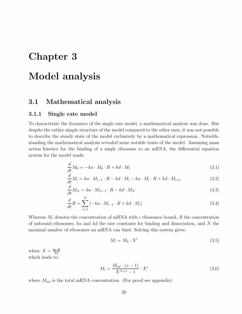
bound ribosomes has the highest concentration (see Figure 3.1).
0 0.2 0.4 0.6 0.8 1 1.2 1.4 1.6 1.8 20
0.1
0.2
0.3
0.4
0.5
0.6
0.7
0.8
0.9
1Change of polysome distribution depending on x
x
conc
unboundmonopoly2poly3poly4poly5
Figure 3.1: The influence of the ratio of X = kaRkd
on the (relative) concentrations of thedifferently loaded mRNAs. The ordering by concentration gives an ascending ribosomal loadingpattern for X < 1, and a descending one for X > 1.
For simulation of the model, this implies that when X crosses 1 during the simulation the
21
distribution pattern of the mRNAs gets inverted. This change may be due to altered values
of ka or kd, which pertains to a regulation of the translation process, of it may be due to the
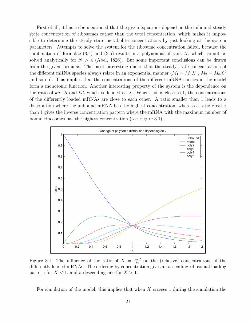
degradation or production of ribosomes. Figure 3.2 gives an example, where the degradation
of ribosomes leads to an inversion of the concentration pattern.
Figure 3.2: Simulation of the single rate model with ribosome degradation (mRNAi = mRNAwith i ribosomes bound) . At time point 25 the value of kaR
kd= X drops below 1 and the order
of the different mRNA concentrations is inverted.
3.1.2 Multiple rate model
The multiple rate model differs from the single rate model only in having distinct initiation
rates for the different translation states. Therefore, the derived formula for the concentration
of each translation state looks rather similar to the one in the single rate model. The steady
state concentration of mRNA with i ribosomes bound in is given by:
Mi = M0 ·i−1∏
j=0
kaj ·(R
kd
)i(3.7)
(For proof see appendix)
It is to mention that the concentration of each translation state depends on all the initiation
rates of the lower transcribed mRNAs, which is not surprising since the ribosomes have to bind
sequentially.
22

3.1.3 Bitstring model
The structure of the rate equations for the bitstring model is rather complicated and hence
it was not possible to solve the rate equations analytically. Nevertheless, the derived rate
equations are given here. In contrast to the single and multiple rate models, Mi denotes not
the concentration of mRNA with i ribosomes bound but rather the concentration of the mRNA
which translation state is represented by the binary string of i. For instance, M2 denotes an
mRNA with a single ribosome bound to the second last position (M00010 for K = 5). K
denotes the maximal number of bound ribosomes, and N = 2K the number of distinct loading
patterns for the mRNA. The rate equations read:
d
dtMi =I(i) · ka ·R ·Mi−2K−1 − T (i) · kd ·Mi +
K−1∑
j=1
e · (A(i, j)−B(i, j)) (3.8)
d
dtR =
N∑
i=1
(−ka ·Mi ·R · I(i) +Mi · kd · T (i)) (3.9)
=
2K−1∑
i=1
−ka ·Mi ·R +
2k−1∑
i=1
kd ·M2i−1
where
N = 2K (3.10)
I(i) =
{1 if bin(i)[1] = 10 else
(3.11)
T (i) =
{1 if bin(i)[K] = 10 else
(3.12)
A(i, j) =
{Mi+2j+1−2j if bin(i)[j] = 0 ∧ bin(i)[j + 1] = 10 else
(3.13)
B(i, j) =
{Mi if bin(i)[j] = 1 ∧ bin(i)[j + 1] = 00 else
(3.14)
and bin(i)[j] denotes the jth position of the binary representation of i
Since these equations are not too obvious, they need a bit of explanation. Formula (3.8)
denotes the time derivation of the concentrations of the different translation states. This
equation is formed by a term for the initiation (I(i) · ka · R ·Mi−2K−1), a negative term for
the termination (−T (i) · kd ·Mi), and a sum over the different elongation reactions (∑K−1
j=1 e ·(A(i, j)−B(i, j)). To understand these terms, one has to keep in mind that i actually denotes
the decimal representation of a binary string. For example, M4 represents the mRNA which
translation state is described by the bitstring 00100 (for K = 5), that means an mRNA with
a single ribosome bound to position 3. An mRNA species can only have been formed by an
initiation reaction, if a ribosome is bound to the first position. This is indicated by I(i), which
23
is 1 if the corresponding mRNA can have been formed by an initiation, and 0 if not. In addition,
an mRNA species that is formed by initiation arises from the mRNA species with the same
bistring representation, with the difference that the first position is 0, whereas it is 1 in the
formed species. Therefore, the mRNA species that forms mRNA species Mi by initiation is
Mi−2K−1 . Thus, the contribution of initiation to the rate change of Mi is the product of the
initiation rate ka, the ribosome concentration R, and the concentration of the uninitialized
mRNA (Mi−2K−1). I(i) just indicates if Mi−2K−1 is defined or not.
The Termination term in formula (3.8) can be explained in a similar way. An mRNA species
can be degraded by termination, if a ribosome is bound to the last position. This is indicated by
T (i). Therefore, the contribution of termination is the product of the mRNA to be terminated
(Mi), the indication if it can be terminated T (i), and the termination rate kd.
The term for the elongation reactions is a bit more complicated. As explained in section
2.1.3, an elongation reaction is represented in the bitstring model by the change of a 10 pattern
to a 01 pattern. Consequently, the degrading contribution of elongation can be described
by a sum over all 10 pattern, and the forming contribution by a sum over all 01 patterns.
Furthermore, a degradation corresponds to the considered mRNA (Mi), whereas a formation
arises from the mRNA where the specific 01 pattern is a 10 pattern. The term B(i, j) gives
Mi if the considered position j in the mRNA Mi is a 10 pattern. That means the degradation
contribution of elongation can be summed up by −∑K−1j=1 e · B(i, j), whereas e denotes the
elongation rate. The function A(i, j) gives the mRNA species from which Mi can be formed in
the initiation reaction if Mi contains a 01 pattern at position i, and 0 otherwise. This mRNA
species is Mi+2j+1−2j , since one is interested in the mRNA concentration where the 0 in the
bitstring at position j is 1 and the 1 at position j+ 1 is 0. Combining these two effects one can
write the elongation contribution as∑K−1
j=1 e · (A(i, j)−B(i, j)).
Equation (3.9) denotes the rate change of the ribosomes. This can be written as a sum over
all mRNA species containing a negative term −ka ·Mi ·R · I(i) for the initiations and a positive
term Mi · kd · T (i) for the terminations. Since an initiation reaction can only take place if the
first position is free, the initiation contribution can be rewritten by the sum over all mRNAs
where the first position is 0 (∑2K−1
i=1 −ka ·Mi ·R). Likewise the termination requires a ribosome
bound to the last position. Therefore, the termination contribution can be written as a sum
over all uneven mRNA species (∑2k−1
i=1 kd ·M2i−1).
3.2 Simulation analysis
The mathematical analysis revealed some properties of the single rate model, but it was not
possible to derive a complete mathematical description for any of the presented models. For this
reason, it seemed sensible to examine the behavior of the different models, by just simulating
them with different parameters. The simulations were done with MATLAB (Matlab, 2005),
which allows simulating any system that can be described by ordinary differential equations
(ODEs). The process of simulating a system in MATLAB is exemplified in the appendix.
24
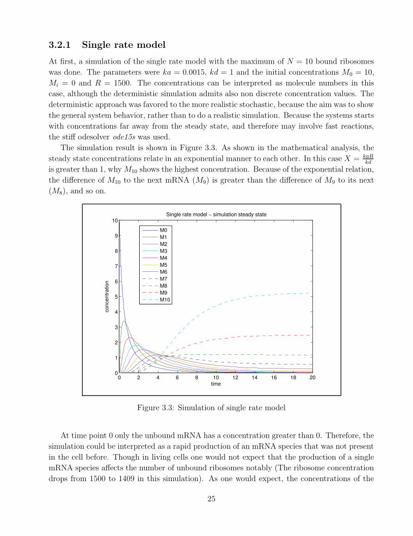
3.2.1 Single rate model
At first, a simulation of the single rate model with the maximum of N = 10 bound ribosomes
was done. The parameters were ka = 0.0015, kd = 1 and the initial concentrations M0 = 10,
Mi = 0 and R = 1500. The concentrations can be interpreted as molecule numbers in this
case, although the deterministic simulation admits also non discrete concentration values. The
deterministic approach was favored to the more realistic stochastic, because the aim was to show
the general system behavior, rather than to do a realistic simulation. Because the systems starts
with concentrations far away from the steady state, and therefore may involve fast reactions,
the stiff odesolver ode15s was used.
The simulation result is shown in Figure 3.3. As shown in the mathematical analysis, the
steady state concentrations relate in an exponential manner to each other. In this case X = kaRkd
is greater than 1, why M10 shows the highest concentration. Because of the exponential relation,
the difference of M10 to the next mRNA (M9) is greater than the difference of M9 to its next
(M8), and so on.
0 2 4 6 8 10 12 14 16 18 200
1
2
3
4
5
6
7
8
9
10
time
conc
entra
tion
Single rate model − simulation steady state
M0M1M2M3M4M5M6M7M8M9M10
Figure 3.3: Simulation of single rate model
At time point 0 only the unbound mRNA has a concentration greater than 0. Therefore, the
simulation could be interpreted as a rapid production of an mRNA species that was not present
in the cell before. Though in living cells one would not expect that the production of a single
mRNA species affects the number of unbound ribosomes notably (The ribosome concentration
drops from 1500 to 1409 in this simulation). As one would expect, the concentrations of the
25
differently loaded mRNAs increases one after another, where the raise is the highest for the
mRNAs increasing first. These are the mRNAs with few ribosomes bound. After this initial
increase, the concentration drops again until the steady state concentration is reached. M8,
M9 and M10 do not show this descend, because on the one hand they have a high steady
state concentration anyway, and on the other hand they reach their maximum not until the
underlying mRNAs have leveled off. As already explained in the in the mathematical analysis,
it is possible to invert the concentration pattern by either increasing kd or by decreasing ka
(Simulation result not shown here).
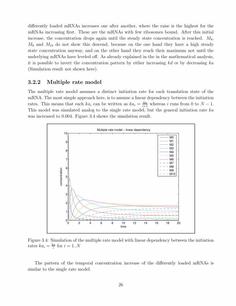
3.2.2 Multiple rate model
The multiple rate model assumes a distinct initiation rate for each translation state of the
mRNA. The most simple approach here, is to assume a linear dependency between the initiation
rates. This means that each kai can be written as kai = kai+1
whereas i runs from 0 to N − 1.
This model was simulated analog to the single rate model, but the general initiation rate ka
was increased to 0.004. Figure 3.4 shows the simulation result.
0 2 4 6 8 10 12 14 16 18 200
1
2
3
4
5
6
7
8
9
10
time
conc
entra
tion
Multiple rate model − linear dependency
M0M1M2M3M4M5M6M7M8M9M10
Figure 3.4: Simulation of the multiple rate model with linear dependency between the initiationrates kai = ka
ifor i = 1..N
The pattern of the temporal concentration increase of the differently loaded mRNAs is
similar to the single rate model.
26
The interesting trait of the multiple rate model is that, in contrast to the single rate model,
the concentrations of the differently loaded mRNAs do not form a monotonic function. There-
fore, M5 has the highest steady state concentration in this simulation. This distribution can not
be reached with a single initiation rate, where the mRNA concentrations relate in a monotonic
pattern (Mi = M0 ·X i). The simulation shows that up to M5 the concentrations increase with
the number of bound ribosomes, whereas it decreases for mRNAs with more than 5 bound
ribosomes.
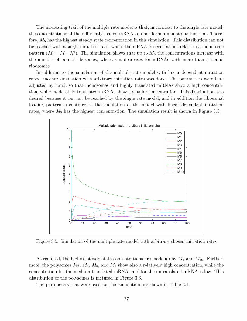
In addition to the simulation of the multiple rate model with linear dependent initiation
rates, another simulation with arbitrary initiation rates was done. The parameters were here
adjusted by hand, so that monosomes and highly translated mRNAs show a high concentra-
tion, while moderately translated mRNAs show a smaller concentration. This distribution was
desired because it can not be reached by the single rate model, and in addition the ribosomal
loading pattern is contrary to the simulation of the model with linear dependent initiation
rates, where M5 has the highest concentration. The simulation result is shown in Figure 3.5.
0 10 20 30 40 50 60 70 80 90 1000
1
2
3
4
5
6
7
8
9
10
time
conc
entra
tion
Multiple rate model − arbitrary initiation rates
M0M1M2M3M4M5M6M7M8M9M10
Figure 3.5: Simulation of the multiple rate model with arbitrary chosen initiation rates
As required, the highest steady state concentrations are made up by M1 and M10. Further-
more, the polysomes M2, M3, M8, and M9 show also a relatively high concentration, while the
concentration for the medium translated mRNAs and for the untranslated mRNA is low. This
distribution of the polysomes is pictured in Figure 3.6.
The parameters that were used for this simulation are shown in Table 3.1.
27

0 1 2 3 4 5 6 7 8 9 100
0.5
1
1.5
2
2.5Multiple rate model − steady state concentrations
conc
entra
tion
number of bound ribosomes
Figure 3.6: Steady state distribution of the polysomes in the simulation shown in Figure 3.5
ka0 ka1 ka2 ka3 ka4 ka5 ka6 ka7 ka8 ka9 kd15 0.0004 0.0005 0.0003 0.0005 0.0009 0.0012 0.0012 0.0009 0.0012 1
Table 3.1: Parameters for simulation 3.5
The initial concentrations were the same as in the previous simulations. Interestingly the
rate constant for the reaction directly forming M1, ka1 is 4 orders of magnitude higher than
the one for the reaction producing M10, which shows a similar steady state concentration. This
is because (i) the polysomal pattern depends not only on the distribution of the ka′s but also
on the ratio of the total mRNA and ribosome concentration, and (ii) the concentration of each
mRNA is not only determined by the rates directly acting on it but also on all the other rates
for the preceding reactions (see Equation (3.7)). This is again reflected in the high value of
ka7, while the proximate rates have a relative low value although the according concentrations
are rather high.
3.2.3 Bitstring model
In contrast to the models examined so far, the bitstring model takes into account interactions
between the ribosomes. The bitstring model has three parameters: the binding constant for
the initiation ka, the rate at which ribosomes move forward one interval e, and the rate at
which ribosomes dissociate when they reach the end of the open reading frame kd. Figure 3.7
shows a simulation result for ka = 0.1, e = 1, and kd = 5. The initial concentrations are again
10 for the untranslated, 0 for all other mRNAs, and 1500 for the ribosome concentration. It
has to be noted that the different translation states are not made up by a single species in this
28
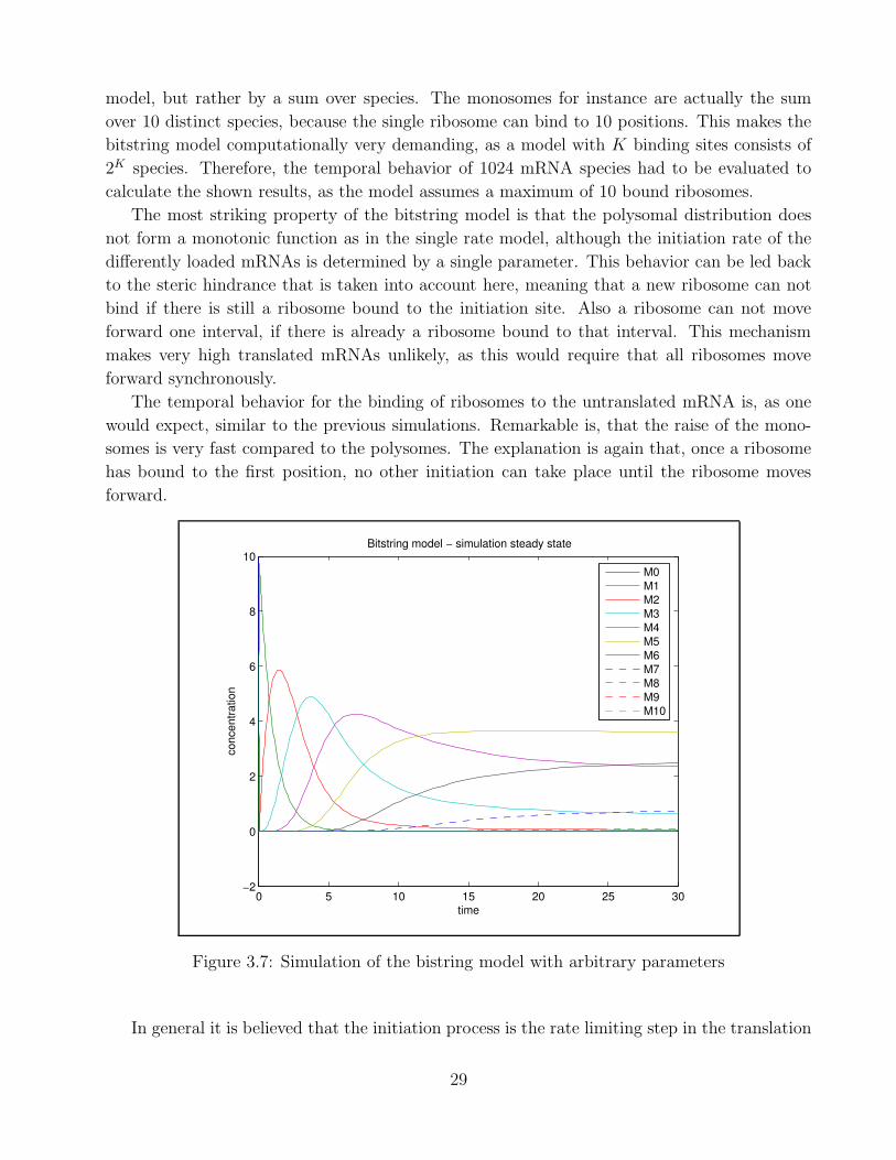
model, but rather by a sum over species. The monosomes for instance are actually the sum
over 10 distinct species, because the single ribosome can bind to 10 positions. This makes the
bitstring model computationally very demanding, as a model with K binding sites consists of
2K species. Therefore, the temporal behavior of 1024 mRNA species had to be evaluated to
calculate the shown results, as the model assumes a maximum of 10 bound ribosomes.
The most striking property of the bitstring model is that the polysomal distribution does
not form a monotonic function as in the single rate model, although the initiation rate of the
differently loaded mRNAs is determined by a single parameter. This behavior can be led back
to the steric hindrance that is taken into account here, meaning that a new ribosome can not
bind if there is still a ribosome bound to the initiation site. Also a ribosome can not move
forward one interval, if there is already a ribosome bound to that interval. This mechanism
makes very high translated mRNAs unlikely, as this would require that all ribosomes move
forward synchronously.
The temporal behavior for the binding of ribosomes to the untranslated mRNA is, as one
would expect, similar to the previous simulations. Remarkable is, that the raise of the mono-
somes is very fast compared to the polysomes. The explanation is again that, once a ribosome
has bound to the first position, no other initiation can take place until the ribosome moves
forward.
0 5 10 15 20 25 30−2
0
2
4
6
8
10
time
conc
entra
tion
Bitstring model − simulation steady state
M0M1M2M3M4M5M6M7M8M9M10
Figure 3.7: Simulation of the bistring model with arbitrary parameters
In general it is believed that the initiation process is the rate limiting step in the translation
29
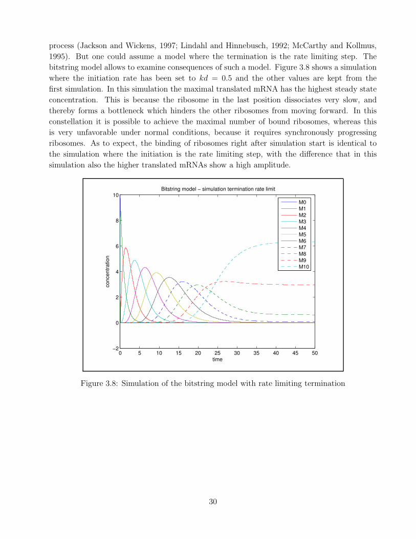
process (Jackson and Wickens, 1997; Lindahl and Hinnebusch, 1992; McCarthy and Kollmus,
1995). But one could assume a model where the termination is the rate limiting step. The
bitstring model allows to examine consequences of such a model. Figure 3.8 shows a simulation
where the initiation rate has been set to kd = 0.5 and the other values are kept from the
first simulation. In this simulation the maximal translated mRNA has the highest steady state
concentration. This is because the ribosome in the last position dissociates very slow, and
thereby forms a bottleneck which hinders the other ribosomes from moving forward. In this
constellation it is possible to achieve the maximal number of bound ribosomes, whereas this
is very unfavorable under normal conditions, because it requires synchronously progressing
ribosomes. As to expect, the binding of ribosomes right after simulation start is identical to
the simulation where the initiation is the rate limiting step, with the difference that in this
simulation also the higher translated mRNAs show a high amplitude.
0 5 10 15 20 25 30 35 40 45 50−2
0
2
4
6
8
10
time
conc
entra
tion
Bitstring model − simulation termination rate limit
M0M1M2M3M4M5M6M7M8M9M10
Figure 3.8: Simulation of the bitstring model with rate limiting termination
30

Chapter 4
Data fit
The aim of this work was to develop a model which is able to explain the temporal pattern
of polysomal association of mRNAs that is found in yeast cells when subjected to osmotic
stress. Therefore, the parameters for different models were adjusted in a way, so that they best
describe the given data. The approach here was to fit the models to a steady state distribution
of polysomes first, and to modify these models subsequently in a way such they can explain
the temporal data.
4.1 Data
The data that the models were fit to are measurements of the polysomal association of the
total mRNA in a cell. This data has been measured as explained in section 1.4.2. These
measurements were done in the Department of Cell and Molecular Biology at the Lundberg
Laboratory, Goteborg University, and were kindly provided for this thesis.
The data that has been used in this section are the measurements of the polysomal profiles
in the yeast cells Saccharomyces cerevisiae in a 10 minute time window after osmotic shock.
Figure 4.1 shows how the translation state of the cell changes after the osmotic shock. The
values for the concentration of mRNA translated by ten or more ribosomes has been pooled in
this data, and also there are no values for the concentration of untranslated mRNA. The value
on the X-axis is not the absolute concentration of the mRNA, but indicates the extinction in
the measurements and thereby the relative concentration.
It can be seen that under normal conditions most mRNA has bound 10 or more ribosomes.
After the osmotic shock this distribution gets shifted, so that most mRNA is translated by
monosomes. The time points 2 and 3 show an intermediate distribution, where both monosomes
and polysomes have a relatively high concentration.
4.2 Used tools
Different tools have been tested to fit the models to the time points, and shall shortly be
described at this point. Mathematically, a parameter fit is an optimization problem that
31

Figure 4.1: The change of the translation state after osmotic shock. The X-axis indicates thenumber of bound ribosomes, and the Y-axis the relative mRNA concentration. After osmoticshock the translation state drops from highly translated polysomes to prevailing monosomes.
minimizes the distances between certain data points and the according points in the model, by
choosing the right parameters. This optimization problem can be tackled by either guessing
the parameters in a smart way, or by directed search algorithms that evaluate the gradient of
the system. In addition, it may be possible do fit the parameters by analytically solving the
system, but this is only possible in few cases.
4.2.1 SBMLpet
SBMLpet (Zi and Klipp, 2006) is a parameter estimation tool that operates on files given in
the Systems Biology Markup Language (Finney and Hucka, 2003) (SBML) format, which is a
standard for the representation of reaction networks. Since all models developed in this thesis
have been implemented in Dizzy (Ramsey et al., 2005), which offers an export to SBML, the
program could have been used to fit all models. SBMLpet translates the SBML model to C
source code, which can be compiled and runs therefore very fast. The program is able to handle
normalized data, where the maximum value of each time point has been scaled to 1. SBMLpet
works well for small SBML models, but importing the bitstring model with 10 binding sites
failed because it was too large. Some models have been fitted with SBMLpet, but since the fits
have been repeated using MATLAB these are favored for better comparability.
4.2.2 Berkeley Madonna
Berkeley Madonna (BM) 1 is a commercial software to simulate systems that are given as
differential equations. In this thesis only the free version of BM has been used, which does not
1http://berkeleymadonna.com
32
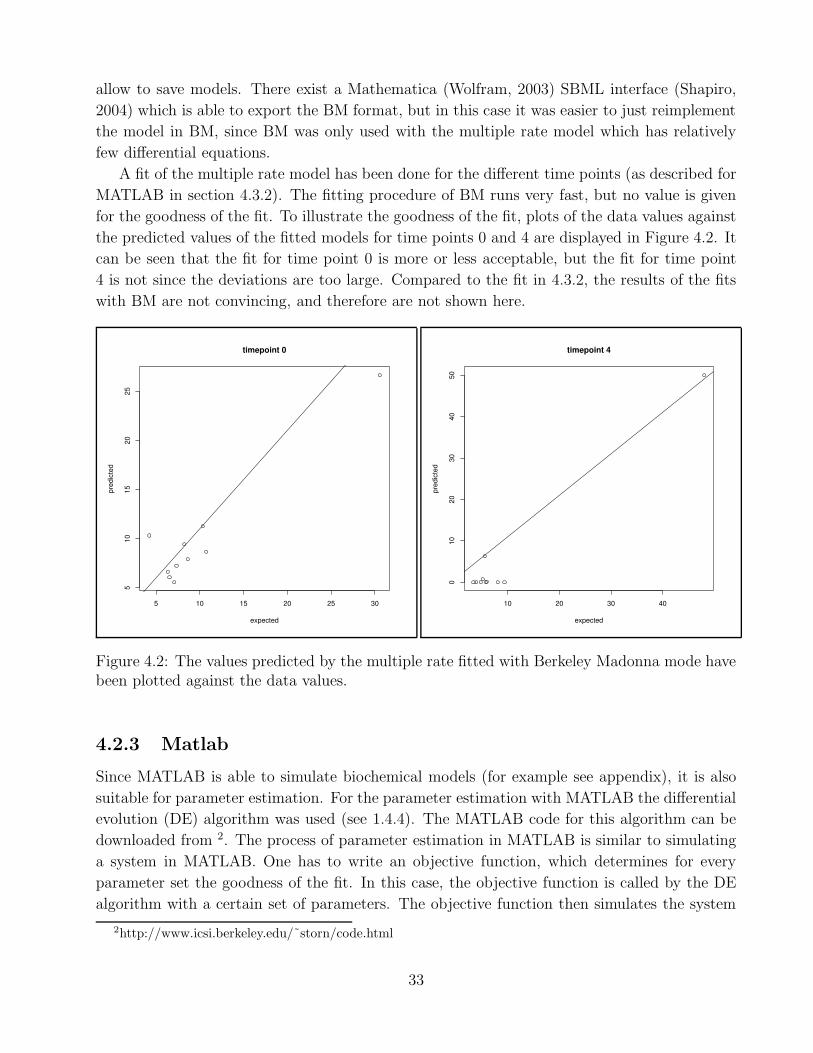
allow to save models. There exist a Mathematica (Wolfram, 2003) SBML interface (Shapiro,
2004) which is able to export the BM format, but in this case it was easier to just reimplement
the model in BM, since BM was only used with the multiple rate model which has relatively
few differential equations.
A fit of the multiple rate model has been done for the different time points (as described for
MATLAB in section 4.3.2). The fitting procedure of BM runs very fast, but no value is given
for the goodness of the fit. To illustrate the goodness of the fit, plots of the data values against
the predicted values of the fitted models for time points 0 and 4 are displayed in Figure 4.2. It
can be seen that the fit for time point 0 is more or less acceptable, but the fit for time point
4 is not since the deviations are too large. Compared to the fit in 4.3.2, the results of the fits
with BM are not convincing, and therefore are not shown here.
5 10 15 20 25 30
510
1520
25
timepoint 0
expected
pred
icte
d
10 20 30 40
010
2030
4050
timepoint 4
expected
pred
icte
d
Figure 4.2: The values predicted by the multiple rate fitted with Berkeley Madonna mode havebeen plotted against the data values.
4.2.3 Matlab
Since MATLAB is able to simulate biochemical models (for example see appendix), it is also
suitable for parameter estimation. For the parameter estimation with MATLAB the differential
evolution (DE) algorithm was used (see 1.4.4). The MATLAB code for this algorithm can be
downloaded from 2. The process of parameter estimation in MATLAB is similar to simulating
a system in MATLAB. One has to write an objective function, which determines for every
parameter set the goodness of the fit. In this case, the objective function is called by the DE
algorithm with a certain set of parameters. The objective function then simulates the system
2http://www.icsi.berkeley.edu/˜storn/code.html
33
for the given parameters, determines the residual sum of squares (RSSQ) at a fixed time point,
and returns this value to the DE function. This is done a lot of times during one parameter fit,
and the best parameters are returned.
Parameter estimation with MATLAB gives the user by far more control over the procedure
than SBMLpet or Berkeley Madonna, since optimization parameters can be specified, the model
can be modified arbitrarily, and certain constraints can be included (This is also possible in
SBMLpet). Because the estimation procedure is also very fast and underlying algorithm and
procedure is known, MATLAB was used for the fits in this section.
4.3 Steady state fit
In the first step the polysomal distribution at different time points was considered as a steady
state distribution. Of course the different time points do not correspond to a steady state,
but this assumption was just accepted to compare the estimated parameter sets for these time
points. This allowed to fit the models to the different time points independently, and to compare
the resulting parameter distribution afterwards. The idea behind this was to derive a temporal
model by looking at how the parameters for the different time points change in the same model.
To adjust the model to the data, at first the data was normalized, so that the sum over
all concentrations equals 100. Since the measurements are relative measurements, the concen-
trations have no unit in this approach. The initial concentrations were chosen in a way that
the total mRNA concentration is 110. The total concentration was chosen higher than it is
in the normalized data, because the data does not include the untranslated mRNA. To fit the
models to the concentration values of the different time points, the differential evolution (DE)
algorithm (see introduction) was used with MATLAB. The DE algorithm requires an objective
function, which determines for every parameter set the quality of the fit. In these cases the
residual sum of squares (RSSQ) between the data and the predicted values at time point 60
were used. It is important to distinguish this simulation time point from the data time points,
since we are considering each of the different time points as a steady state distribution. This
time point was used, since it was assumed that 60 time steps are sufficient for the system to
reach a stable distribution.
4.3.1 Single rate model
The single rate model has been fit to all six time points. The monotonic structure of the model
implies that no satisfiable fit to a non monotonic polysomal distribution can be found. Time
points 2 and 3 show such a monotonic distribution. Since the polysomes with 10 or more
ribosomes bound have been pooled in the data, it was assumed in the model, that maximal 16
ribosomes can bind to one mRNA, and the concentrations were pooled together for polysomes
consisting out of 10 or more ribosomes. The initial concentrations have been chosen to be11017≈ 6.47 for each translation state (including untranslated mRNA).
34
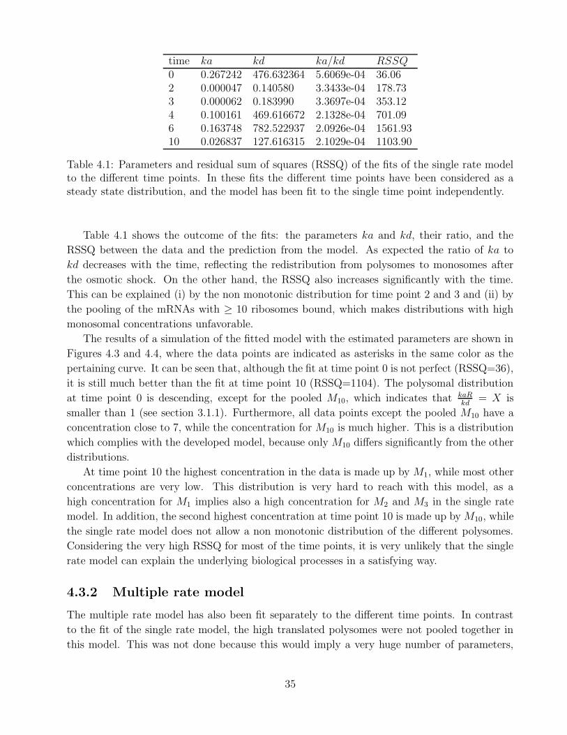
time ka kd ka/kd RSSQ0 0.267242 476.632364 5.6069e-04 36.062 0.000047 0.140580 3.3433e-04 178.733 0.000062 0.183990 3.3697e-04 353.124 0.100161 469.616672 2.1328e-04 701.096 0.163748 782.522937 2.0926e-04 1561.9310 0.026837 127.616315 2.1029e-04 1103.90
Table 4.1: Parameters and residual sum of squares (RSSQ) of the fits of the single rate modelto the different time points. In these fits the different time points have been considered as asteady state distribution, and the model has been fit to the single time point independently.
Table 4.1 shows the outcome of the fits: the parameters ka and kd, their ratio, and the
RSSQ between the data and the prediction from the model. As expected the ratio of ka to
kd decreases with the time, reflecting the redistribution from polysomes to monosomes after
the osmotic shock. On the other hand, the RSSQ also increases significantly with the time.
This can be explained (i) by the non monotonic distribution for time point 2 and 3 and (ii) by
the pooling of the mRNAs with ≥ 10 ribosomes bound, which makes distributions with high
monosomal concentrations unfavorable.
The results of a simulation of the fitted model with the estimated parameters are shown in
Figures 4.3 and 4.4, where the data points are indicated as asterisks in the same color as the
pertaining curve. It can be seen that, although the fit at time point 0 is not perfect (RSSQ=36),
it is still much better than the fit at time point 10 (RSSQ=1104). The polysomal distribution
at time point 0 is descending, except for the pooled M10, which indicates that kaRkd
= X is
smaller than 1 (see section 3.1.1). Furthermore, all data points except the pooled M10 have a
concentration close to 7, while the concentration for M10 is much higher. This is a distribution
which complies with the developed model, because only M10 differs significantly from the other
distributions.
At time point 10 the highest concentration in the data is made up by M1, while most other
concentrations are very low. This distribution is very hard to reach with this model, as a
high concentration for M1 implies also a high concentration for M2 and M3 in the single rate
model. In addition, the second highest concentration at time point 10 is made up by M10, while
the single rate model does not allow a non monotonic distribution of the different polysomes.
Considering the very high RSSQ for most of the time points, it is very unlikely that the single
rate model can explain the underlying biological processes in a satisfying way.
4.3.2 Multiple rate model
The multiple rate model has also been fit separately to the different time points. In contrast
to the fit of the single rate model, the high translated polysomes were not pooled together in
this model. This was not done because this would imply a very huge number of parameters,
35

0 0.05 0.1 0.15 0.2 0.25 0.3 0.35 0.4 0.45 0.50
5
10
15
20
25
30
35
40
45
50
time
conc
entra
tion
Single rate model − fit time point 0
M1M2M3M4M5M6M7M8M9>M10M1M2M3M4M5M6M7M8M9>M10
Figure 4.3: Simulation of the single rate model with the parameters estimated for time point0. The data points are shown as asterisks in the same color as the pertaining curve.
since in the multiple rate model each translation state has it’s own initiation rate. The initial
concentrations were 10 for each mRNA species, which gives a total mRNA concentration of
110, and again 1500 for the ribosomes. The result of the parameter estimation is shown in
Table 4.2.
As to be seen, the model explains the data in an almost perfect way, since no RSSQ has a
higher value than 1. Indeed this was to expect, because a model with 11 parameters should be
able to explain 10 data points. On the other hand, all the velocity constants are very high, which
indicates very fast reactions. This is not very realistic, but results from the objective function
that does not discriminate very high reaction constants. The parameters are also shown in a
normalized way, where the highest value of each time point (the dissociation rate) has been
rescaled to 1. These normalized values can be compared with each other, and make more sense
in a biological way than the extremely high reaction constants derived from the DE algorithm.
The differences in the errors between the normalized and unnormalized parameters may be due
to rounding errors, since Equation (3.7) indicates that linear rescaling of all parameters should
not affect the polysomal steady state distribution.
The initiation rates are much smaller than the dissociation rates in this fit, but this should
not be interpreted because the ratio of the both depends on the concentration of total mRNA
and ribosomes, which were chosen arbitrary in this case. Looking into the differences in the
36
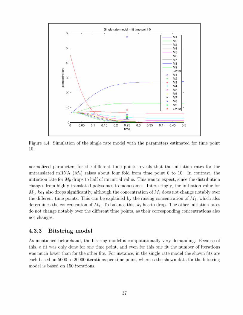
0 0.05 0.1 0.15 0.2 0.25 0.3 0.35 0.4 0.45 0.50
10
20
30
40
50
60
time
conc
entra
tion
Single rate model − fit time point 0
M1M2M3M4M5M6M7M8M9>M10M1M2M3M4M5M6M7M8M9>M10
Figure 4.4: Simulation of the single rate model with the parameters estimated for time point10.
normalized parameters for the different time points reveals that the initiation rates for the
untranslated mRNA (M0) raises about four fold from time point 0 to 10. In contrast, the
initiation rate for M9 drops to half of its initial value. This was to expect, since the distribution
changes from highly translated polysomes to monosomes. Interestingly, the initiation value for
M1, ka1 also drops significantly, although the concentration of M2 does not change notably over
the different time points. This can be explained by the raising concentration of M1, which also
determines the concentration of M2. To balance this, k1 has to drop. The other initiation rates
do not change notably over the different time points, as their corresponding concentrations also
not changes.
4.3.3 Bitstring model
As mentioned beforehand, the bistring model is computationally very demanding. Because of
this, a fit was only done for one time point, and even for this one fit the number of iterations
was much lower than for the other fits. For instance, in the single rate model the shown fits are
each based on 5000 to 20000 iterations per time point, whereas the shown data for the bitstring
model is based on 150 iterations.
37
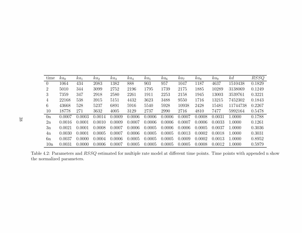
time ka0 ka1 ka2 ka3 ka4 ka5 ka6 ka7 ka8 ka9 kd RSSQ0 1064 434 2083 1382 888 903 957 1047 1187 4637 1510438 0.18292 5010 344 3099 2752 2196 1795 1739 2175 1885 10289 3138069 0.12493 7359 347 2918 2580 2261 1911 2253 2158 1945 13003 3539761 0.32214 22168 538 3915 5151 4432 3623 3488 9550 1716 13215 7452302 0.18436 43668 528 5237 6891 5916 5540 5928 10938 2428 15481 11744738 0.226710 18778 271 3632 4005 3129 2737 2990 2716 4810 7477 5992164 0.54780n 0.0007 0.0003 0.0014 0.0009 0.0006 0.0006 0.0006 0.0007 0.0008 0.0031 1.0000 0.17882n 0.0016 0.0001 0.0010 0.0009 0.0007 0.0006 0.0006 0.0007 0.0006 0.0033 1.0000 0.12613n 0.0021 0.0001 0.0008 0.0007 0.0006 0.0005 0.0006 0.0006 0.0005 0.0037 1.0000 0.30364n 0.0030 0.0001 0.0005 0.0007 0.0006 0.0005 0.0005 0.0013 0.0002 0.0018 1.0000 0.30316n 0.0037 0.0000 0.0004 0.0006 0.0005 0.0005 0.0005 0.0009 0.0002 0.0013 1.0000 0.895210n 0.0031 0.0000 0.0006 0.0007 0.0005 0.0005 0.0005 0.0005 0.0008 0.0012 1.0000 0.5979
Table 4.2: Parameters and RSSQ estimated for multiple rate model at different time points. Time points with appended n showthe normalized parameters.
38
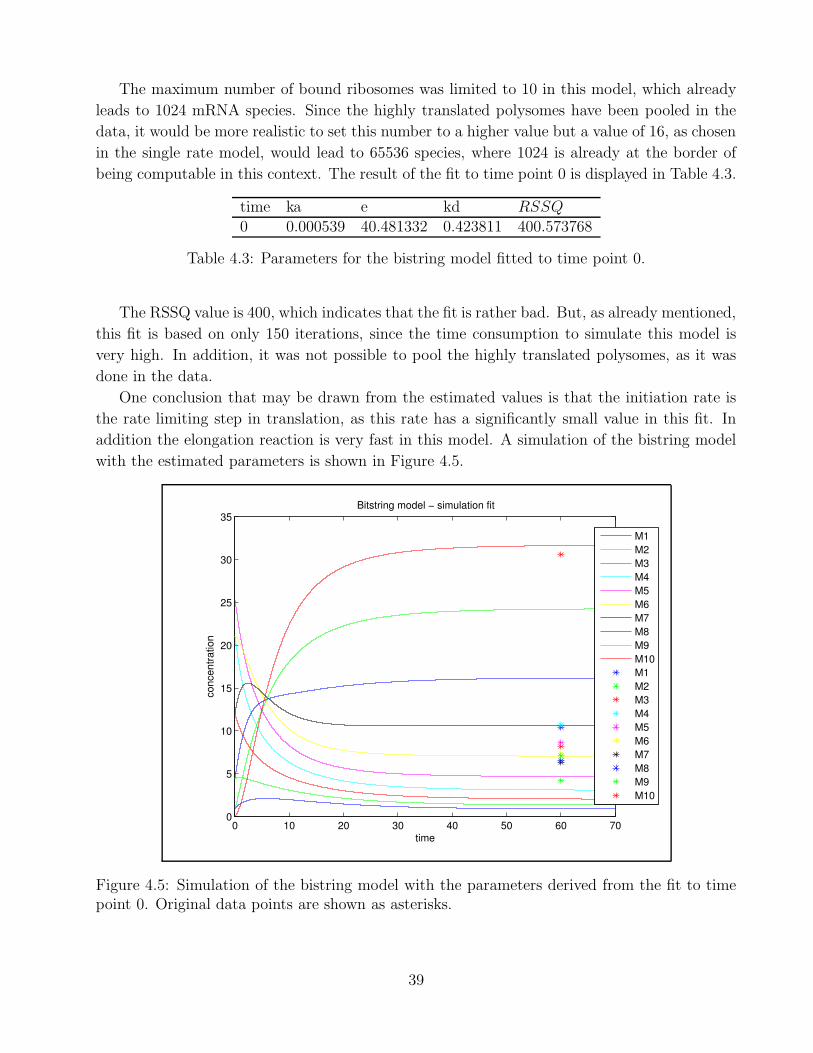
The maximum number of bound ribosomes was limited to 10 in this model, which already
leads to 1024 mRNA species. Since the highly translated polysomes have been pooled in the
data, it would be more realistic to set this number to a higher value but a value of 16, as chosen
in the single rate model, would lead to 65536 species, where 1024 is already at the border of
being computable in this context. The result of the fit to time point 0 is displayed in Table 4.3.
time ka e kd RSSQ0 0.000539 40.481332 0.423811 400.573768
Table 4.3: Parameters for the bistring model fitted to time point 0.
The RSSQ value is 400, which indicates that the fit is rather bad. But, as already mentioned,
this fit is based on only 150 iterations, since the time consumption to simulate this model is
very high. In addition, it was not possible to pool the highly translated polysomes, as it was
done in the data.
One conclusion that may be drawn from the estimated values is that the initiation rate is
the rate limiting step in translation, as this rate has a significantly small value in this fit. In
addition the elongation reaction is very fast in this model. A simulation of the bistring model
with the estimated parameters is shown in Figure 4.5.
0 10 20 30 40 50 60 700
5
10
15
20
25
30
35
time
conc
entra
tion
Bitstring model − simulation fit
M1M2M3M4M5M6M7M8M9M10M1M2M3M4M5M6M7M8M9M10
Figure 4.5: Simulation of the bistring model with the parameters derived from the fit to timepoint 0. Original data points are shown as asterisks.
39
4.4 Time course fit
The modes that have been fitted in the previous section were constructed to describe a steady
state distribution of polysomes. Originating from these separated fits to the single time points,
the aim was to develop a model that can explain the temporal behavior of the translation state
after the osmotic shock. Because one could imagine different explanations for the translation
state response after osmotic shock, these explanations were incorporated into the models, and
the models were fit to the time course data. At the end, the different possible explanations
were compared.
Two different approaches were chosen to fit the data: First, an additional reaction that may
explain the change in the polysomal profile was added to the multiple rate model, whereas the
parameters were kept from the previous fit to time point 0. In addition, a simplified multiple
rate model with a lower number of parameters was fitted to the time course data. This second
approach was not based on the previous steady state fits, but instead all parameters were
guessed by the DE algorithm. The bitstring model was not used to derive a time course model
because it was not possible to simulate it in an appropriate time, whereas the single rate model
was not used because of its inability to explain the steady state data.
The additional reaction (or parameter change), that was supposed to explain the temporal
data, was chosen to set in after the system has found a steady state. Therefore this reaction
did not act before time point 50, wherefore time point 50 pertains to time point 0 in the data.
The time scale was the same as in the data, so time point 52 pertains to time point 2 in the
data, and so on. This means that the data fit was only done in the interval [50 60]. Since the
time scale is in minutes in the data, this scale applies also to the models.
4.4.1 Multiple rate model
In the first approach, the multiple rate model was modified in a way that it may explain the
data. The parameters and initial concentrations were taken from the previous steady state
fit to time point 0, but in addition a reaction producing mRNA, or degrading ribosomes was
included. Because only one reaction was added and the other parameters were taken from the
preceding step, only one parameter had to be guessed by the estimation algorithm.
mRNA concentration change
The first model examined was the production of mRNA. Since the measured data gives no
information about the total mRNA concentration, one could imagine that mRNA production
leads to a redistribution of poly- and monosomes. A biological basis for this assumption is not
given. Nevertheless, one would expect a shift from polysomes to monosomes in response to an
mRNA production, since the available amount of ribosomes is shared between more mRNA.
To examine the goodness of such a model explaining the time course data, it was implemented
and fitted. The model used for this fit was the multiple rate model, with the parameters and
initial concentrations from the fit to time point 0. In addition, a reaction producing mRNA
40
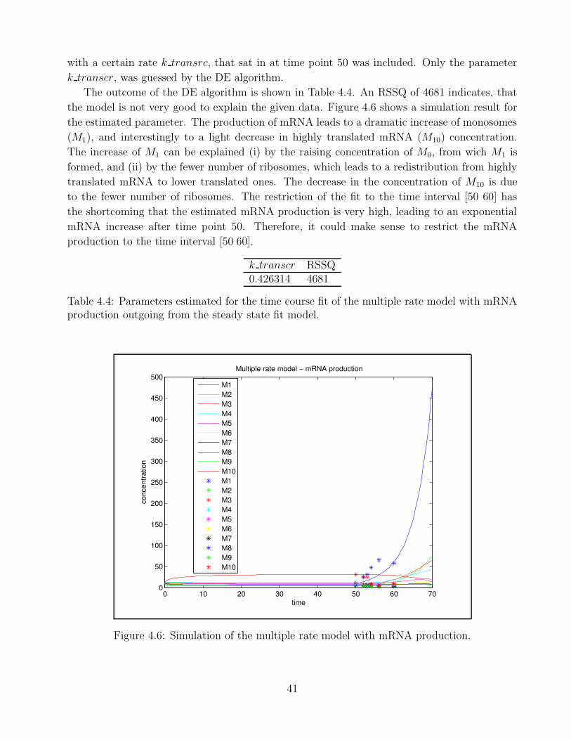
with a certain rate k transrc, that sat in at time point 50 was included. Only the parameter
k transcr, was guessed by the DE algorithm.
The outcome of the DE algorithm is shown in Table 4.4. An RSSQ of 4681 indicates, that
the model is not very good to explain the given data. Figure 4.6 shows a simulation result for
the estimated parameter. The production of mRNA leads to a dramatic increase of monosomes
(M1), and interestingly to a light decrease in highly translated mRNA (M10) concentration.
The increase of M1 can be explained (i) by the raising concentration of M0, from wich M1 is
formed, and (ii) by the fewer number of ribosomes, which leads to a redistribution from highly
translated mRNA to lower translated ones. The decrease in the concentration of M10 is due
to the fewer number of ribosomes. The restriction of the fit to the time interval [50 60] has
the shortcoming that the estimated mRNA production is very high, leading to an exponential
mRNA increase after time point 50. Therefore, it could make sense to restrict the mRNA
production to the time interval [50 60].
k transcr RSSQ0.426314 4681
Table 4.4: Parameters estimated for the time course fit of the multiple rate model with mRNAproduction outgoing from the steady state fit model.
0 10 20 30 40 50 60 700
50
100
150
200
250
300
350
400
450
500
time
conc
entra
tion
Multiple rate model − mRNA production
M1M2M3M4M5M6M7M8M9M10M1M2M3M4M5M6M7M8M9M10
Figure 4.6: Simulation of the multiple rate model with mRNA production.
41

Ribosome concentration change
In the mathematical analysis it has been shown that a degradation of ribosomes can invert
the concentration pattern in the single rate model. Therefore, one could expect that this
rearrangement from polysomes to monosomes also takes place in the multiple rate model, if
the ribosome concentration drops below a certain value. This approach has also been tested.
The procedure was analog to the test of the mRNA production, with the difference that the
reaction that produced mRNA was replaced by a reaction that degrades ribosomes with rate
R · k degr.The result of the fit is shown in Table 4.5 and a simulation with the estimated parameters
is shown in Figure 4.7. The RSSQ of almost 7000 indicates that this model is not able to
explain the data. As to be seen in the simulation, the degradation of ribosomes leads to a rapid
concentration decrease of the highly translated mRNA M10. In addition, the concentration of
the monosomes M1 shows a light increase, which is by far not as strong as in the data. Likewise
a light increase in the beginning of the degradation can be seen for the less translated mRNAs
M2 and M3. The other polysomes show a decrease, since the available number of ribosomes
gets smaller. Summing up it can be said that the increase of monosomes derived from the
ribosome degradation is not strong enough to mimic the data. In contrast, the drop of highly
translates polysomes (M10) is similar in the model and in the data.
k degr RSSQ0.23579 6927
Table 4.5: Parameters estimated for the time course fit of the multiple rate model with ribosomedegradation outgoing from the steady state fit model.
4.4.2 Model with 3 initiation rates
In addition to the multiple rate model originating from the fit to time point 0, a hybrid of the
single rate model and the multiple rate model was used, where the different translation states
were split into three groups with different initiation rates. In this approach the untranslated
mRNA M0, the mRNAs M1 to M10 and the mRNAs M11 to M16 made each up one group. The
mRNAs M10 to M16 were pooled together in the model, because also in the data the highly
translated mRNAs had been pooled. The main difference to the previous fit is that in this case
all model parameters are guessed, and no information from the previous fitted steady state is
taken into account.
Initiation rate change
One could imagine that the drop from polysomes to monosomes after osmotic shock is due
to a regulation of the initiation. Therefore a model was implemented, where the initiation
rate drops linear with the time. This would correspond to a slow regulation of the initiation
42
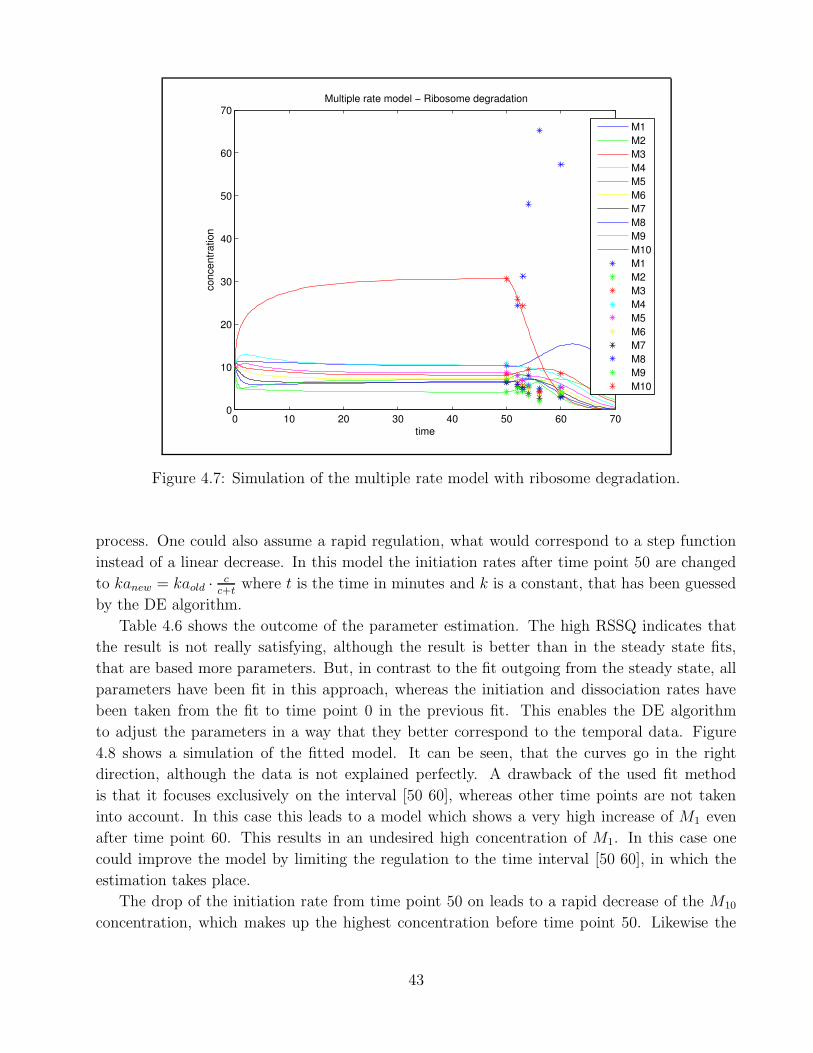
0 10 20 30 40 50 60 700
10
20
30
40
50
60
70
time
conc
entra
tion
Multiple rate model − Ribosome degradation
M1M2M3M4M5M6M7M8M9M10M1M2M3M4M5M6M7M8M9M10
Figure 4.7: Simulation of the multiple rate model with ribosome degradation.
process. One could also assume a rapid regulation, what would correspond to a step function
instead of a linear decrease. In this model the initiation rates after time point 50 are changed
to kanew = kaold · cc+t
where t is the time in minutes and k is a constant, that has been guessed
by the DE algorithm.
Table 4.6 shows the outcome of the parameter estimation. The high RSSQ indicates that
the result is not really satisfying, although the result is better than in the steady state fits,
that are based more parameters. But, in contrast to the fit outgoing from the steady state, all
parameters have been fit in this approach, whereas the initiation and dissociation rates have
been taken from the fit to time point 0 in the previous fit. This enables the DE algorithm
to adjust the parameters in a way that they better correspond to the temporal data. Figure
4.8 shows a simulation of the fitted model. It can be seen, that the curves go in the right
direction, although the data is not explained perfectly. A drawback of the used fit method
is that it focuses exclusively on the interval [50 60], whereas other time points are not taken
into account. In this case this leads to a model which shows a very high increase of M1 even
after time point 60. This results in an undesired high concentration of M1. In this case one
could improve the model by limiting the regulation to the time interval [50 60], in which the
estimation takes place.
The drop of the initiation rate from time point 50 on leads to a rapid decrease of the M10
concentration, which makes up the highest concentration before time point 50. Likewise the
43
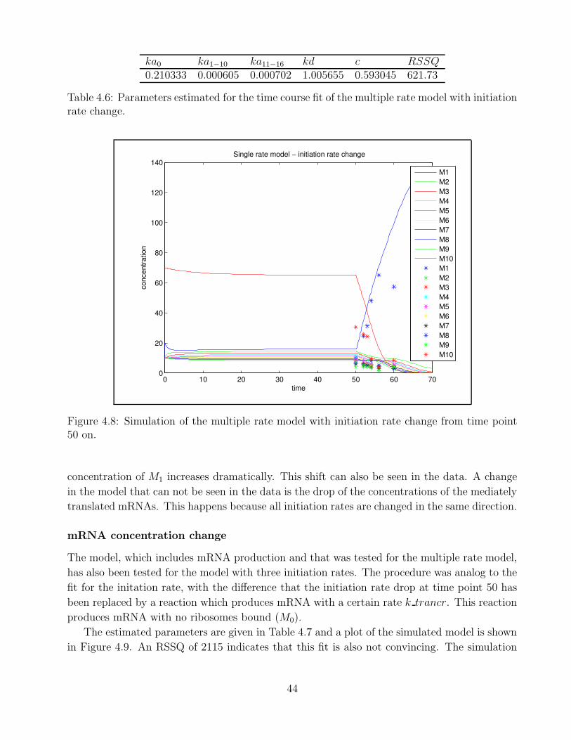
ka0 ka1−10 ka11−16 kd c RSSQ0.210333 0.000605 0.000702 1.005655 0.593045 621.73
Table 4.6: Parameters estimated for the time course fit of the multiple rate model with initiationrate change.
0 10 20 30 40 50 60 700
20
40
60
80
100
120
140
time
conc
entra
tion
Single rate model − initiation rate change
M1M2M3M4M5M6M7M8M9M10M1M2M3M4M5M6M7M8M9M10
Figure 4.8: Simulation of the multiple rate model with initiation rate change from time point50 on.
concentration of M1 increases dramatically. This shift can also be seen in the data. A change
in the model that can not be seen in the data is the drop of the concentrations of the mediately
translated mRNAs. This happens because all initiation rates are changed in the same direction.
mRNA concentration change
The model, which includes mRNA production and that was tested for the multiple rate model,
has also been tested for the model with three initiation rates. The procedure was analog to the
fit for the initation rate, with the difference that the initiation rate drop at time point 50 has
been replaced by a reaction which produces mRNA with a certain rate k trancr. This reaction
produces mRNA with no ribosomes bound (M0).
The estimated parameters are given in Table 4.7 and a plot of the simulated model is shown
in Figure 4.9. An RSSQ of 2115 indicates that this fit is also not convincing. The simulation
44
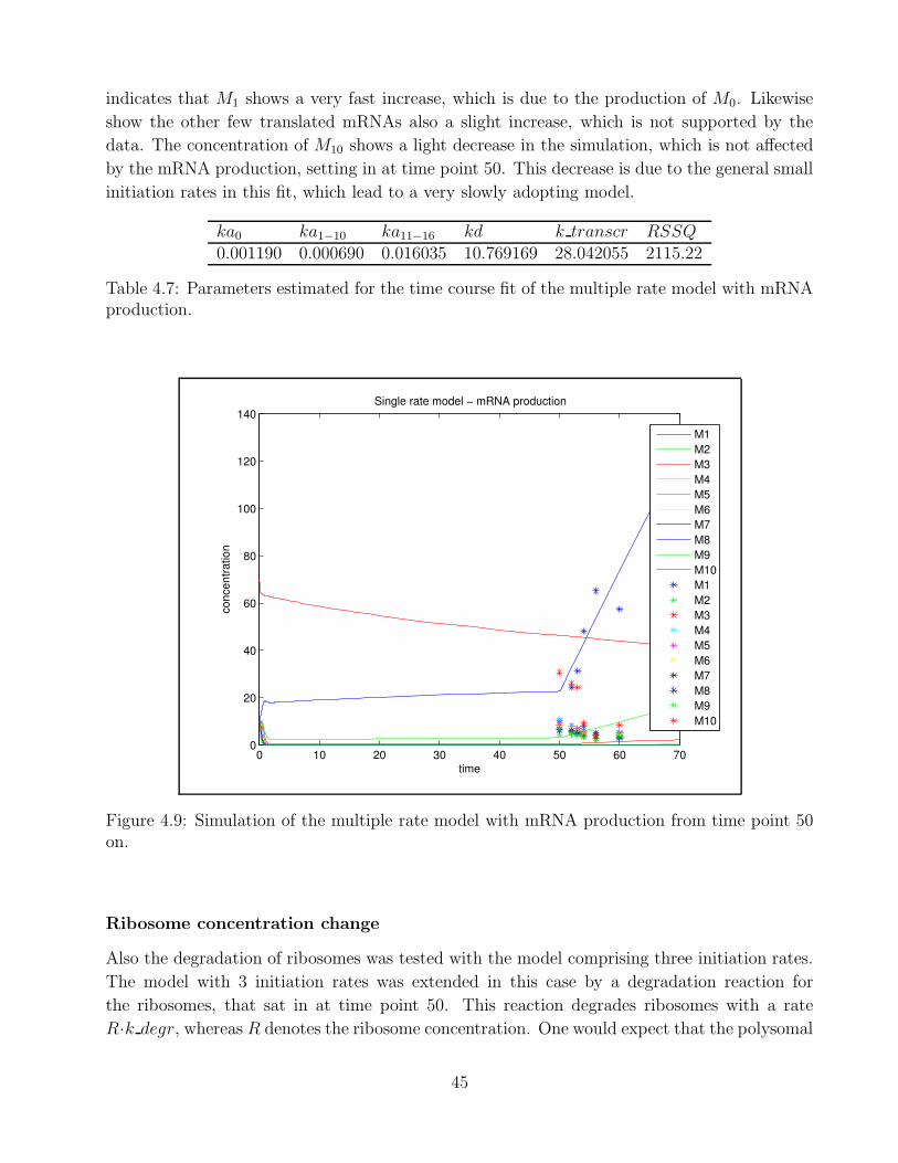
indicates that M1 shows a very fast increase, which is due to the production of M0. Likewise
show the other few translated mRNAs also a slight increase, which is not supported by the
data. The concentration of M10 shows a light decrease in the simulation, which is not affected
by the mRNA production, setting in at time point 50. This decrease is due to the general small
initiation rates in this fit, which lead to a very slowly adopting model.
ka0 ka1−10 ka11−16 kd k transcr RSSQ0.001190 0.000690 0.016035 10.769169 28.042055 2115.22
Table 4.7: Parameters estimated for the time course fit of the multiple rate model with mRNAproduction.
0 10 20 30 40 50 60 700
20
40
60
80
100
120
140
time
conc
entra
tion
Single rate model − mRNA production
M1M2M3M4M5M6M7M8M9M10M1M2M3M4M5M6M7M8M9M10
Figure 4.9: Simulation of the multiple rate model with mRNA production from time point 50on.
Ribosome concentration change
Also the degradation of ribosomes was tested with the model comprising three initiation rates.
The model with 3 initiation rates was extended in this case by a degradation reaction for
the ribosomes, that sat in at time point 50. This reaction degrades ribosomes with a rate
R·k degr, whereas R denotes the ribosome concentration. One would expect that the polysomal
45
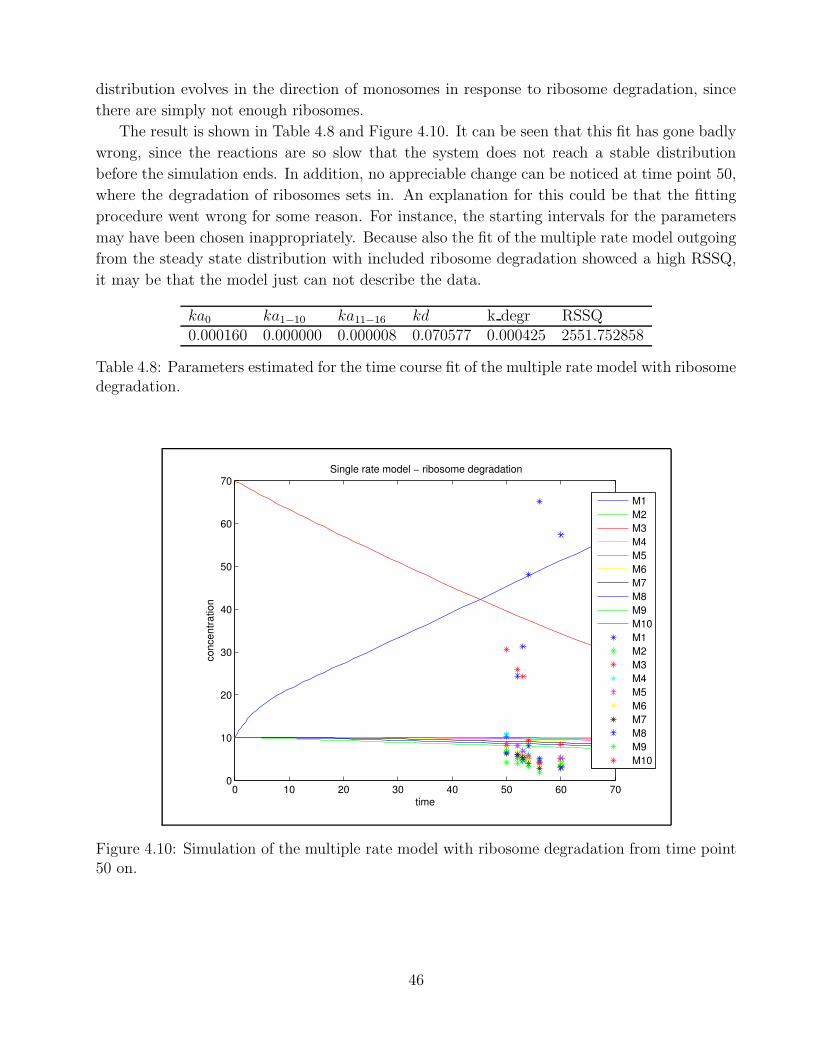
distribution evolves in the direction of monosomes in response to ribosome degradation, since
there are simply not enough ribosomes.
The result is shown in Table 4.8 and Figure 4.10. It can be seen that this fit has gone badly
wrong, since the reactions are so slow that the system does not reach a stable distribution
before the simulation ends. In addition, no appreciable change can be noticed at time point 50,
where the degradation of ribosomes sets in. An explanation for this could be that the fitting
procedure went wrong for some reason. For instance, the starting intervals for the parameters
may have been chosen inappropriately. Because also the fit of the multiple rate model outgoing
from the steady state distribution with included ribosome degradation showced a high RSSQ,
it may be that the model just can not describe the data.
ka0 ka1−10 ka11−16 kd k degr RSSQ0.000160 0.000000 0.000008 0.070577 0.000425 2551.752858
Table 4.8: Parameters estimated for the time course fit of the multiple rate model with ribosomedegradation.
0 10 20 30 40 50 60 700
10
20
30
40
50
60
70
time
conc
entra
tion
Single rate model − ribosome degradation
M1M2M3M4M5M6M7M8M9M10M1M2M3M4M5M6M7M8M9M10
Figure 4.10: Simulation of the multiple rate model with ribosome degradation from time point50 on.
46
Chapter 5
Results
5.1 Comparison
In this work, different models have been developed and prospected with regard to different pro-
cesses explaining the change in polysomal profiles, that is found when yeast cells are subjected
to osmotic stress. At this point, the different models, and the different probed processes shall
be compared for their quality to explain the given data.
5.1.1 Models
Three models have been examined: (i) the single rate model, where the initiation rate does not
depend on the number of bound ribosomes, (ii) the multiple rate model, where this is adverse,
and (iii) the bitstring model, that takes into account the position of each ribosome on the
mRNA.
Single rate model
The single rate model has a fairly simple structure, and is therefore only able to describe
a monotonic pattern of the ribosomal association. This means that it is not able to form a
distribution where both monosomes and highly translated polysomes have a high concentration,
while mildly translated polysomes have a low concentration. For this reason the single rate
model has not been used to construct a temporal model. The simple structure of this model
has the advantage that at least some conclusions can be drawn from a mathematical analysis
(e.g. monotonic structure, turning point). Though a complete mathematical description, for
instance to fit the model analytically to data points, could not be derived.
Multiple rate model
The multiple rate model is an extension of the single rate model, where every translation state
of the mRNA has its own rate for binding to a ribosome. This leads to a model with a lot
of parameters, and it is questionable if this assumption is meaningful in a biological context.
47
Nevertheless, the multiple rate model is able to mimic the distributions of the measurements
at the different time points in an almost perfect manner. Because of the enormous number of
parameters, this had to be expected.
Two modifications of this model outgoing from the fit to the data at time point 0 were not
able to mimic the temporal polysomal profile after the osmotic shock. This may be reducible,
either to an inability of the model or of the examined processes to describe the data. An answer
to this question would require a deeper analysis of the model and the processes.
In addition to the fit outgoing from a steady state distribution, a simplified version of the
multiple rate model has been fit to the time course data, where all parameters have been esti-
mated. In this simplified model the different translation states of the mRNAs were divided into
three groups. Compared to the fit outgoing from the steady state distribution, this approach
gives a better result, although it is still not satisfying. The explanation for this may be that
all parameters are guessed in this approach, whereas in the first approach a fixed distribution
was modified by a single influence.
Bitstring model
The bitstring model is the most complicated of the presented, since it simulates the binding
position of each single ribosome to the mRNA. Because of this precision the model is very
complex, and therefore could not be solved analytically. In addition, this complexity makes
the model computationally very demanding to simulate. Therefore, it was not possible to fit
this model to time courses, and also the fit to a steady state distribution was only possible in a
limited way. This fit to a steady state distribution led to an inferior fit compared to the other
models. But since the number of iterations of the estimation algorithm was much smaller in
this case, the results are not comparable. The bitstring model is not restricted to a monotonic
loading pattern as the single rate model, although all translation states have the same initiation
rate in this model (not considering the states where a ribosome occupies the initiation site).
5.1.2 Processes
Different processes have been tested in this work that could explain the temporal change in the
polysomal profile in response to osmotic stress. They have been incorporated into the multiple
rate model and fitted to the time course data. The ability of the different processes to describe
the data is compared in this section.
mRNA production
A process that might explain the polysomal profile change after osmotic shock would be an
increase in the mRNA concentration. From the biological point of view this assumption is
doubtful, since the mRNA level is believed to decrease after osmotic shock (Hohmann, 2002).
Nevertheless, this assumption has been tested by implementing it into the multiple rate model,
and fitting this model to the data. The mRNA production hypothesis was tested outgoing from
48
a steady state distribution, as well as by fitting all model parameters. In both cases the result
was not satisfying, since the mRNA production can explain the increase of the monosomes
but not the decrease of the highly translated polysomes. In addition, the mRNA concentration
increased dramatically in the fitted model, which is not possible in such an extend in the reality.
Ribosome degradation
The second model that has been tested was a degradation of ribosomes. In the model outgoing
from the steady state fit this could explain the drop of highly translated polysomes, but not
the increase in monosomes. In the model where all parameters have been fit, this hypothesis
led to a completely wrong model. This may be either because the model can not explain the
data, or because the method to fit the data was inadequate. An improvement of the fit method
would be to require the model to find a steady state before fitting the parameters, since the
simulation in Figure 4.8 shows that this was not the case in this parameter fit.
Initiation rate change
A process that has only been examined outgoing from the model with three initiation rates
was a drop in the initiation rate during the simulation. This corresponds to a regulation in
the translation initiation process, which has been shown to exist (Kimball, 2001). In fact, this
initiation rate change leads to a better result than the other analyzed processes. The initiation
rate drop leads to a redistribution, where the concentration of highly translated polysomes
drops and the concentration of monosomes increases. On the other hand, the concentration of
mediate translated mRNAs drops as well, which is not supported by the data.
5.2 Validation
In addition to global translation state data, array data about the translation state of single genes
was available. This data has been kindly provided by the Department of Cell and Molecular
Biology at the Lundberg Laboratory, Goteborg University. In this data the polysomal and
total mRNA of cells that have been subjected to osmotic stress were measured with DNA
microarrays. Precisely spoken, the polysomal and total mRNA of stressed cells have been
compared to total mRNA of unstressed cells. This was done by two channel arrays (see section
1.4.1). A more detailed analysis of this data was not part of this work, but some results
are displayed and compared to a simulation result. Figure 5.1 shows three different clusters
of a hierarchical clustering of the delta PAFs derived from the array analysis. PAF stand for
polysomal association factor, and denotes the ratio of polysomal to total abundance of a certain
mRNA species. The ratio of the PAF at two time points is called delta PAF. This delta PAF
is shown in Figure 5.1 in a illustrated and quantified way for three differently regulated mRNA
clusters. Because the delta PAFs are all compared to time point 0, the fist value has always
a value of 0, since it is compared to itself. The values are displayed in dual logarithmic scale,
thus a value of 1 denotes a upregulation of factor 2 compared to time point 0.
49
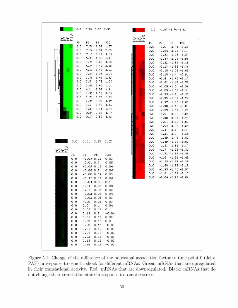
Figure 5.1: Change of the difference of the polysomal association factor to time point 0 (deltaPAF) in response to osmotic shock for different mRNAs. Green: mRNAs that are upregulatedin their translational activity. Red: mRNAs that are downregulated. Black: mRNAs that donot change their translation state in response to osmotic stress.
50
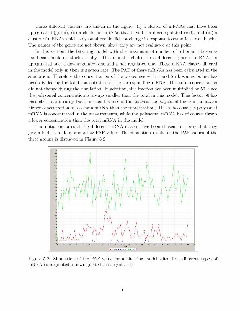
Three different clusters are shown in the figure: (i) a cluster of mRNAs that have been
upregulated (green), (ii) a cluster of mRNAs that have been downregulated (red), and (iii) a
cluster of mRNAs which polysomal profile did not change in response to osmotic stress (black).
The names of the genes are not shown, since they are not evaluated at this point.
In this section, the bitstring model with the maximum of number of 5 bound ribosomes
has been simulated stochastically. This model includes three different types of mRNA, an
upregulated one, a downregulated one and a not regulated one. These mRNA classes differed
in the model only in their initiation rate. The PAF of these mRNAs has been calculated in the
simulation. Therefore the concentration of the polysomes with 4 and 5 ribosomes bound has
been divided by the total concentration of the corresponding mRNA. This total concentration
did not change during the simulation. In addition, this fraction has been multiplied by 50, since
the polysomal concentration is always smaller than the total in this model. This factor 50 has
been chosen arbitrarily, but is needed because in the analysis the polysomal fraction can have a
higher concentration of a certain mRNA than the total fraction. This is because the polysomal
mRNA is concentrated in the measurements, while the polysomal mRNA has of course always
a lower concentration than the total mRNA in the model.
The initiation rates of the different mRNA classes have been chosen, in a way that they
give a high, a middle, and a low PAF value. The simulation result for the PAF values of the
three groups is displayed in Figure 5.2.
Figure 5.2: Simulation of the PAF value for a bitstring model with three different types ofmRNA (upregulated, donwregulated, not regulated)
51

Figure 5.3: Simulation bitstring model upregulated mRNA
It has to be pointed out that the values in Figure 5.1 are delta PAF values, and denote
a temporal change of the translation state. Since in this simulation only a steady state is
considered, it can not be compared directly to the delta PAFs. One could derive delta PAFs
from this model by implementing a temporal change in the initiation rates and taking the
fraction of the PAFs at different time points. This simulation was only meant to illustrate the
polysomal distributions, which lead to different PAF values. Therefore the polysomal profiles of
the different mRNA classes in this simulation are shown in Figures 5.3, 5.4, and 5.5. As already
mentioned, the initiation rates have been chosen in way, that the PAF distribution forms three
different classes. Figure 5.3 shows the upregulated class with a PAF of about 8 (no logarithmic
scale). As one would expect, most of the mRNAs in this class have 5 ribosomes bound. Figure
5.4 shows the simulation for the downregulated class, which has a PAF of about 0.1, and forms
an adverse distribution where the highest concentration is made up by untranslated mRNA.
Figure 5.5 shows the simulation result for the mRNA class which has a PAF at around 1, that
has not been regulated. In addition, this simulation shows that the stochastic noise is bigger
in the PAF values, than in the mRNA concentrations.
52
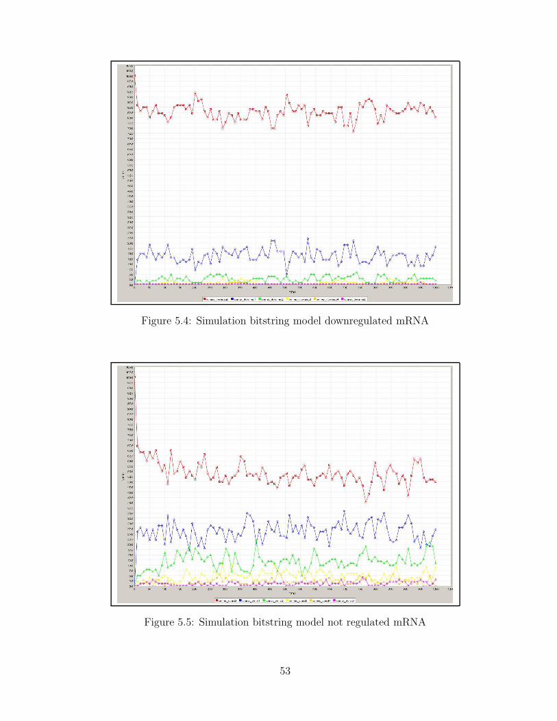
Figure 5.4: Simulation bitstring model downregulated mRNA
Figure 5.5: Simulation bitstring model not regulated mRNA
53
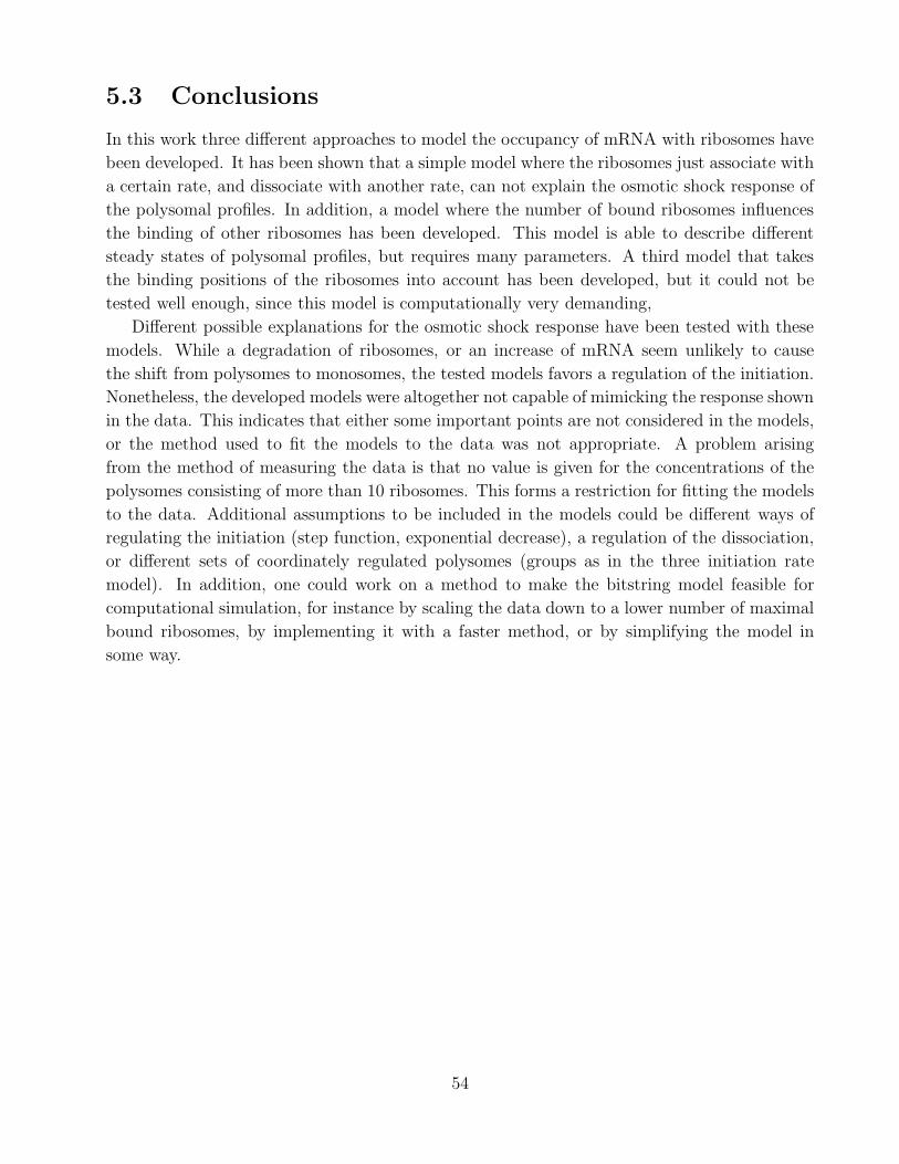
5.3 Conclusions
In this work three different approaches to model the occupancy of mRNA with ribosomes have
been developed. It has been shown that a simple model where the ribosomes just associate with
a certain rate, and dissociate with another rate, can not explain the osmotic shock response of
the polysomal profiles. In addition, a model where the number of bound ribosomes influences
the binding of other ribosomes has been developed. This model is able to describe different
steady states of polysomal profiles, but requires many parameters. A third model that takes
the binding positions of the ribosomes into account has been developed, but it could not be
tested well enough, since this model is computationally very demanding,
Different possible explanations for the osmotic shock response have been tested with these
models. While a degradation of ribosomes, or an increase of mRNA seem unlikely to cause
the shift from polysomes to monosomes, the tested models favors a regulation of the initiation.
Nonetheless, the developed models were altogether not capable of mimicking the response shown
in the data. This indicates that either some important points are not considered in the models,
or the method used to fit the models to the data was not appropriate. A problem arising
from the method of measuring the data is that no value is given for the concentrations of the
polysomes consisting of more than 10 ribosomes. This forms a restriction for fitting the models
to the data. Additional assumptions to be included in the models could be different ways of
regulating the initiation (step function, exponential decrease), a regulation of the dissociation,
or different sets of coordinately regulated polysomes (groups as in the three initiation rate
model). In addition, one could work on a method to make the bitstring model feasible for
computational simulation, for instance by scaling the data down to a lower number of maximal
bound ribosomes, by implementing it with a faster method, or by simplifying the model in
some way.
54
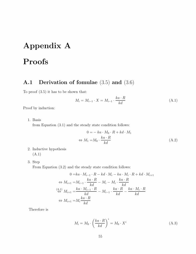
Appendix A
Proofs
A.1 Derivation of fomulae (3.5) and (3.6)
To proof (3.5) it has to be shown that:
Mi = Mi−1 ·X = Mi−1 ·ka ·Rkd
(A.1)
Proof by induction:
1. Basis
from Equation (3.1) and the steady state condition follows:
0 =− ka ·M0 ·R + kd ·M1
⇔M1 =M0 ·ka ·Rkd
(A.2)
2. Inductive hypothesis
(A.1)
3. Step
From Equation (3.2) and the steady state condition follows:
0 =ka ·Mi−1 ·R− kd ·Mi − ka ·Mi ·R + kd ·Mi+1
⇔Mi+1 =Mi−1 ·ka ·Rkd
−Mi −Mi ·ka ·Rkd
(A.1)⇔ Mi+1 =ka ·Mi−1 ·R
kd−Mi−1 ·
ka ·Rkd
− ka ·Mi ·Rkd
⇔Mi+1 =Mika ·Rkd
Therefore is
Mi = M0 ·(ka ·Rkd
)i= M0 ·X i (A.3)
55
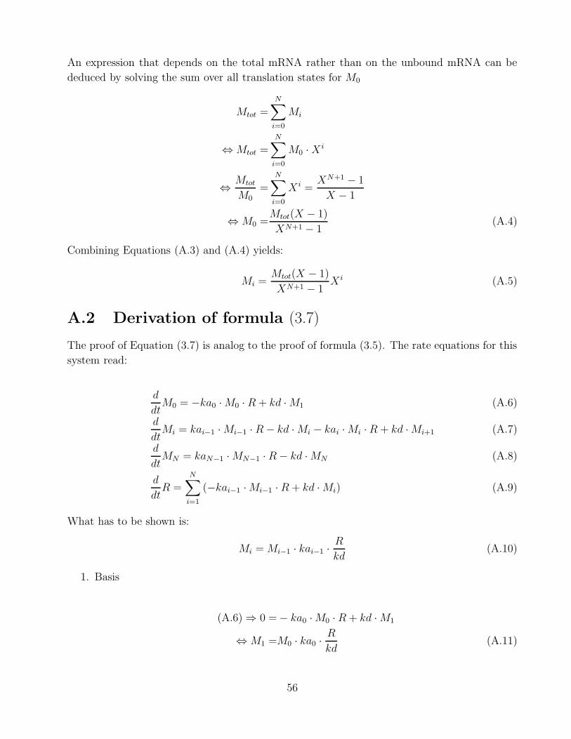
An expression that depends on the total mRNA rather than on the unbound mRNA can be
deduced by solving the sum over all translation states for M0
Mtot =
N∑
i=0
Mi
⇔Mtot =N∑
i=0
M0 ·X i
⇔ Mtot
M0=
N∑
i=0
X i =XN+1 − 1
X − 1
⇔M0 =Mtot(X − 1)
XN+1 − 1(A.4)
Combining Equations (A.3) and (A.4) yields:
Mi =Mtot(X − 1)
XN+1 − 1X i (A.5)
A.2 Derivation of formula (3.7)
The proof of Equation (3.7) is analog to the proof of formula (3.5). The rate equations for this
system read:
d
dtM0 = −ka0 ·M0 ·R + kd ·M1 (A.6)
d
dtMi = kai−1 ·Mi−1 ·R− kd ·Mi − kai ·Mi ·R + kd ·Mi+1 (A.7)
d
dtMN = kaN−1 ·MN−1 ·R− kd ·MN (A.8)
d
dtR =
N∑
i=1
(−kai−1 ·Mi−1 ·R + kd ·Mi) (A.9)
What has to be shown is:
Mi = Mi−1 · kai−1 ·R
kd(A.10)
1. Basis
(A.6)⇒ 0 =− ka0 ·M0 ·R + kd ·M1
⇔M1 =M0 · ka0 ·R
kd(A.11)
56
2. Inductive hypothesis
(A.10)
3. Step
(A.7)⇒ 0 =kai−1 ·Mi−1 ·R− kd ·Mi − kai ·Mi ·R + kd ·Mi+1
⇔Mi+1 =− kai−1 ·Mi−1 ·R
kd+Mi + kai ·Mi ·
R
kd(A.10)⇔ Mi+1 =− kai−1 ·Mi−1 ·
R
kd+Mi−1 · kai−1 ·
R
kd+ kai ·Mi ·
R
kd
⇔Mi+1 =kai ·Mi ·R
kd(A.12)
From (A.12) it follows that (3.7) is true.
57
Appendix B
Deterministic simulation in MATLAB
The change over time of the concentrations of the species in a biochemical system can be
described by a set of ordinary differential equations (ODEs). The change of each species
at a specific time point can be expressed by a gradient function that depends on all other
concentrations, on the parameters and on the time.
d
dtXi = −
∫
i
(X1, ..., XM , p1, ..., pk, t), i = 1...M (B.1)
A general way to derive ODEs for a biochemical system is described in the introduction. A
way to simulate a system is to integrate these equations for certain parameters and initial
concentrations numerically. Numerically integrating a system means to repetitively calculate
the gradient of the single rate model, and update the system values accordingly. This gives an
approximation of how the system would evolve.
To numerically integrate a system in MATLAB a function is required, that calculates the
gradient from the present metabolite concentrations and parameters. A function that does
this for the single rate model with maximum of 10 bound ribosomes is given Figure B.1. This
function calculates the gradient of the system according to Equations (3.1), (3.2), (3.3), and
(3.4) and takes the time t, the concentration vector x and the parameter vector p as input. To
make a simulation with this gradient function one needs to specify initial concentration values
and a set of parameters. Figure B.2 gives an example how this is done in MATLAB. The plot
that is produced by this function is shown in figure 3.3. Because some of the reactions may be
fast in the beginning, where the system converges toward a steady state, the stiff ODE solver
ode15s was used. The different ODE solvers included in MATLAB are listed in the MATLAB
documentation 1.
1http://www.mathworks.com/access/helpdesk/help/techdoc/ref/ode15s.html
58
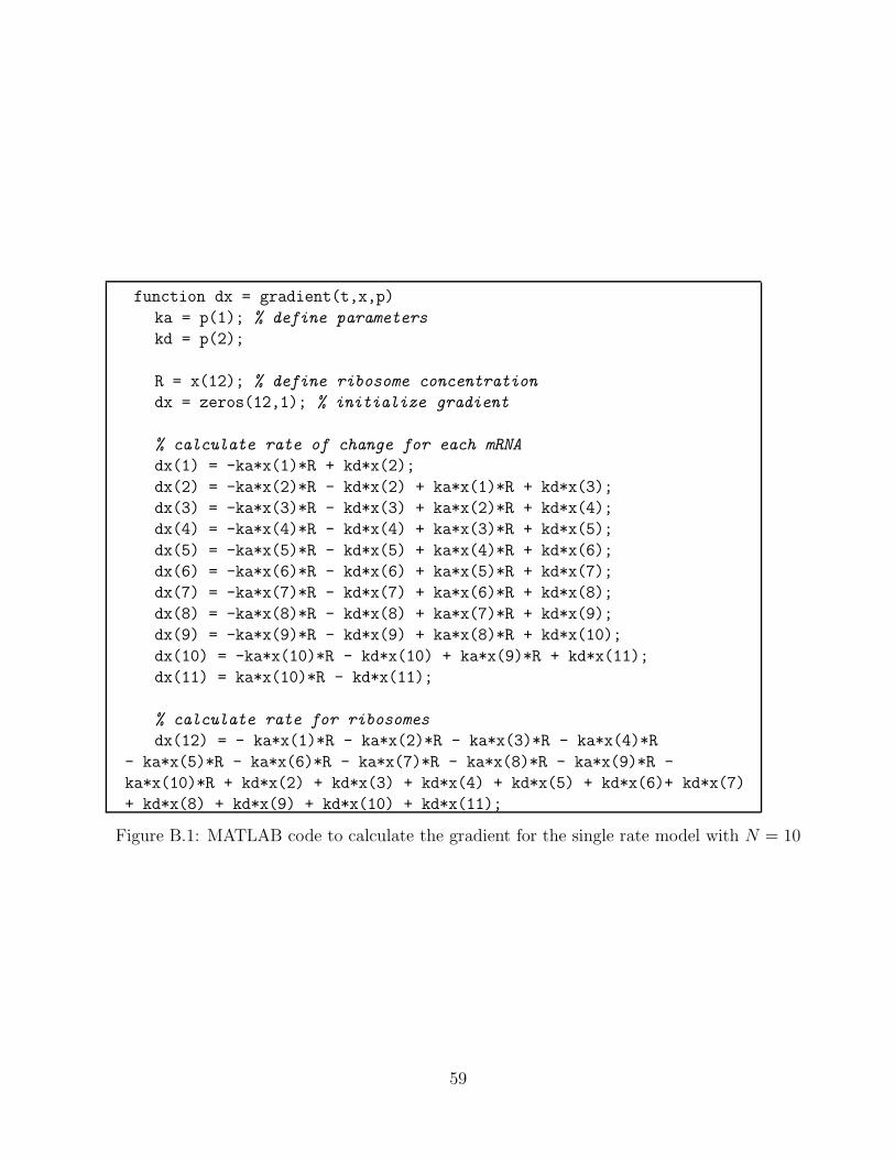
function dx = gradient(t,x,p)
ka = p(1); % define parameters
kd = p(2);
R = x(12); % define ribosome concentration
dx = zeros(12,1); % initialize gradient
% calculate rate of change for each mRNA
dx(1) = -ka*x(1)*R + kd*x(2);
dx(2) = -ka*x(2)*R - kd*x(2) + ka*x(1)*R + kd*x(3);
dx(3) = -ka*x(3)*R - kd*x(3) + ka*x(2)*R + kd*x(4);
dx(4) = -ka*x(4)*R - kd*x(4) + ka*x(3)*R + kd*x(5);
dx(5) = -ka*x(5)*R - kd*x(5) + ka*x(4)*R + kd*x(6);
dx(6) = -ka*x(6)*R - kd*x(6) + ka*x(5)*R + kd*x(7);
dx(7) = -ka*x(7)*R - kd*x(7) + ka*x(6)*R + kd*x(8);
dx(8) = -ka*x(8)*R - kd*x(8) + ka*x(7)*R + kd*x(9);
dx(9) = -ka*x(9)*R - kd*x(9) + ka*x(8)*R + kd*x(10);
dx(10) = -ka*x(10)*R - kd*x(10) + ka*x(9)*R + kd*x(11);
dx(11) = ka*x(10)*R - kd*x(11);
% calculate rate for ribosomes
dx(12) = - ka*x(1)*R - ka*x(2)*R - ka*x(3)*R - ka*x(4)*R
- ka*x(5)*R - ka*x(6)*R - ka*x(7)*R - ka*x(8)*R - ka*x(9)*R -
ka*x(10)*R + kd*x(2) + kd*x(3) + kd*x(4) + kd*x(5) + kd*x(6)+ kd*x(7)
+ kd*x(8) + kd*x(9) + kd*x(10) + kd*x(11);
Figure B.1: MATLAB code to calculate the gradient for the single rate model with N = 10
59
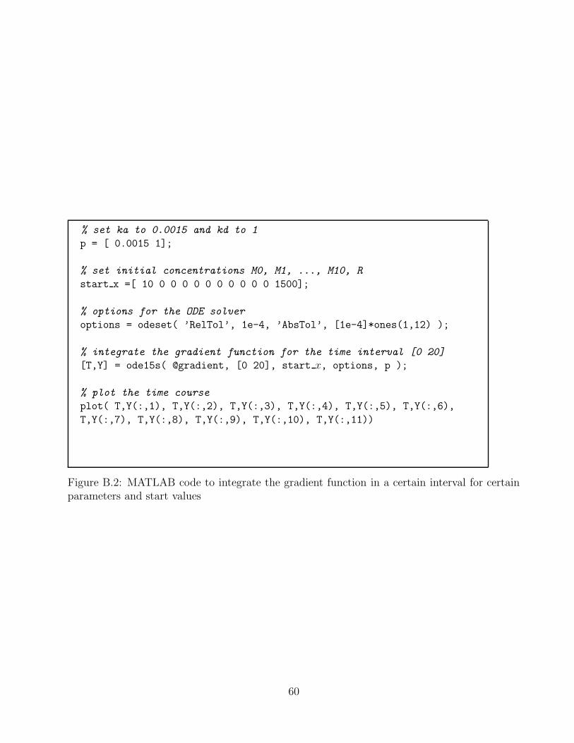
% set ka to 0.0015 and kd to 1
p = [ 0.0015 1];
% set initial concentrations M0, M1, ..., M10, R
start x =[ 10 0 0 0 0 0 0 0 0 0 0 1500];
% options for the ODE solver
options = odeset( ’RelTol’, 1e-4, ’AbsTol’, [1e-4]*ones(1,12) );
% integrate the gradient function for the time interval [0 20]
[T,Y] = ode15s( @gradient, [0 20], start x, options, p );
% plot the time course
plot( T,Y(:,1), T,Y(:,2), T,Y(:,3), T,Y(:,4), T,Y(:,5), T,Y(:,6),
T,Y(:,7), T,Y(:,8), T,Y(:,9), T,Y(:,10), T,Y(:,11))
Figure B.2: MATLAB code to integrate the gradient function in a certain interval for certainparameters and start values
60
Bibliography
Abel, N. (1826). Beweis der Unmoglichkeit algebraische Gleichungen von hoheren Graden als
dem vierten allgemein aufzulosen. J. reine angew. Math, 1:65–84.
Alberts, B., Johnson, A., Lewis, J., Raff, M., Roberts, K., and P., W. (2002). Molecular
Biology of the Cell. Garland Science.
Albertyn, J., Hohmann, S., and Prior, B. (1994). Characterization of the osmotic-stress
response inSaccharomyces cerevisiae: osmotic stress and glucose repression regulate glycerol-
3-phosphate dehydrogenase independently. Current Genetics, 25(1):12–18.
Arava, Y., Wang, Y., Storey, J. D., Liu, C. L., Brown, P. O., and Herschlag, D. (2003).
Genome-wide analysis of mRNA translation profiles in Saccharomyces cerevisiae. Proc Natl
Acad Sci U S A, 100(7):3889–3894.
Ashe, M., De Long, S., and Sachs, A. (2000). Glucose Depletion Rapidly Inhibits Translation
Initiation in Yeast. Molecular Biology of the Cell, 11:833–848.
Bentley, D. (1995). Regulation of transcriptional elongation by RNA polymerase II. Curr.
Opin. Genet. Dev, 5:210–216.
Bernstein, P. and Ross, J. (1989). Poly(A), poly(A) binding protein and the regulation of
mRNA stability. Trends Biochem Sci, 14(9):373–377.
Black, D. L. (2000). Protein diversity from alternative splicing: A challenge for bioinformatics
and post-genome biology. Cell.
Blomberg, A. and Adler, L. (1992). Physiology of osmotolerance in fungi. Adv Microb Physiol,
33:145–212.
Brown, V., Jin, P., Ceman, S., Darnell, J., ODonnell, W., Tenenbaum, S., Jin, X., Feng, Y.,
Wilkinson, K., Keene, J., et al. (2001). Microarray identification of FMRP-associated brain
mRNAs and altered mRNA translational profiles in fragile X syndrome. Cell, 107(4):477–487.
Causton, H., Ren, B., Koh, S., Harbison, C., Kanin, E., Jennings, E., Lee, T., True, H.,
Lander, E., and Young, R. (2001). Remodeling of Yeast Genome Expression in Response to
Environmental Changes. Molecular Biology of the Cell, 12:323–337.
61

Conaway, R. C. and Conaway, J. W. (1993). General initiation factors for RNA polymerase
II. Annu Rev Biochem, 62:161–190.
Daneholt, B. (1997). A look at messenger RNP moving through the nuclear pore. Cell,
88(5):585–588.
Deschenes, R. J., Lin, H., Ault, A. D., and Fassler, J. S. (1999). Antifungal properties and
target evaluation of three putative bacterial histidine kinase inhibitors. Antimicrob Agents
Chemother, 43(7):1700–1703.
Dickson, L. (1998). mRNA translation in yeast during entry into stationary phase. Molecular
and General Genetics MGG, 259(3):282–293.
Ding, D. and Lipshitz, H. (1993). Localized RNAs and their functions. Bioessays, 15(10):651–
8.
Drummond, D. R., Armstrong, J., and Colman, A. (1985). The effect of capping and
polyadenylation on the stability, movement and translation of synthetic messenger RNAs
in Xenopus oocytes. Nucleic Acids Res, 13(20):7375–7394.
Eddy, S. R. (1999). Noncoding RNA genes. Curr Opin Genet Dev, 9(6):695–699.
Estruch, F. (2000). Stress-controlled transcription factors, stress-induced genes and stress
tolerance in budding yeast. FEMS Microbiol Rev, 24(4):469–86.
Finney, A. and Hucka, M. (2003). Systems biology markup language: Level 2 and beyond.
Biochem Soc Trans, 31(Pt 6):1472–1473.
Francois, J. and Parrou, J. (2001). Reserve carbohydrates metabolism in the yeast Saccha-
romyces cerevisiae. FEMS Microbiol Rev, 25(1):125–45.
Gasch, A., Spellman, P., Kao, C., Carmel-Harel, O., Eisen, M., Storz, G., Botstein, D.,
and Brown, P. (2000). Genomic Expression Programs in the Response of Yeast Cells to
Environmental Changes. Science’s STKE, 11(12):4241–4257.
Gibson, M. and Bruck, J. (2000). Efficient exact stochastic simulation of chemical systems
with many species and many channels. J. Phys. Chem. A, 104(9):1876–1889.
Gillespie, D. (1977). Exact stochastic simulation of coupled chemical reactions. The Journal
of Physical Chemistry, 81(25):2340–2361.
Goffeau, A., Barrell, B. G., Bussey, H., Davis, R. W., Dujon, B., Feldmann, H., Galibert, F.,
Hoheisel, J. D., Jacq, C., Johnston, M., Louis, E. J., Mewes, H. W., Murakami, Y., Philippsen,
P., Tettelin, H., and Oliver, S. G. (1996). Life with 6000 genes. Science, 274(5287):563–567.
Gurdon, J. B. (1968). Changes in somatic cell nuclei inserted into growing and maturing
amphibian oocytes. J Embryol Exp Morphol, 20(3):401–414.
62
Heinrich, R. and Rapoport, T. (1974). A linear steady-state treatment of enzymatic chains.
General properties, control and effector strength. Eur J Biochem, 42(1):89–95.
Helliwell, S., Wagner, P., Kunz, J., Deuter-Reinhard, M., Henriquez, R., and Hall, M. (1994).
TOR1 and TOR2 are structurally and functionally similar but not identical phosphatidylinos-
itol kinase homologues in yeast. Mol. Biol. Cell, 5:105–118.
Herrick, D., Parker, R., and Jacobson, A. (1990). Identification and comparison of stable and
unstable mRNAs in Saccharomyces cerevisiae. Molecular and Cellular Biology, 10(5):2269–
2284.
Hirayarna, T., Maeda, T., Saito, H., and Shinozaki, K. (1995). Cloning and characterization
of seven cDNAs for hyperosmolarity-responsive (HOR) genes of Saccharomyces cerevisiae.
Molecular Genetics and Genomics, 249(2):127–138.
Hohmann, S. (2002). Osmotic stress signaling and osmoadaptation in yeasts. Microbiol Mol
Biol Rev, 66(2):300–372.
Hounsa, C. G., Brandt, E. V., Thevelein, J., Hohmann, S., and Prior, B. A. (1998). Role of
trehalose in survival of Saccharomyces cerevisiae under osmotic stress. Microbiology, 144 ( Pt
3):671–680.
Huang, Y. and Carmichael, G. C. (1996). Role of polyadenylation in nucleocytoplasmic trans-
port of mRNA. Mol Cell Biol, 16(4):1534–1542.
Jackson, R. and Wickens, M. (1997). Translational controls impinging on the 5’-untranslated
region and initiation factor proteins. Curr. Opin. Genet. Dev, 7(2):233–241.
Jacobson, A., Brown, A., Donahue, J., Herrick, D., Parker, R., and Peltz, S. (1990). Regulation
of mRNA stability in yeast. NATO ASI Ser. Ser. H, 49:45–54.
Jacobson, A. and Peltz, S. (1996). Interrelationships of the Pathways of mRNA Decay and
Translation in Eukaryotic Cells. Annual Review of Biochemistry, 65(1):693–739.
Johannes, G., Carter, M., Eisen, M., Brown, P., and Sarnow, P. (1999). Identification of
eukaryotic mRNAs that are translated at reduced cap binding complex eIF4F concentrations
using a cDNA microarray. Proceedings of the National Academy of Sciences, 96(23):13118–
13123.
Kacser, H. and Burns, J. (1973). The control of flux. Symp. Soc. Exp. Biol, 27(65):104.
Kimball, S. (2001). Regulation of translation initiation by amino acids in eukaryotic cells.
Prog Mol Subcell Biol, 26:155–84.
Kingston, R. (1999). ATP-dependent remodeling and acetylation as regulators of chromatin
fluidity. Genes & Development, 13(18):2339–2352.
63
Kitano, H. (2002). Systems Biology: A Brief Overview. Science, 295(5560):1662–1664.
Klipp, E., Herwig, R., Kowald, A., Wierling, C., and Lehrach, H. (2005a). Systems Biology
in Practice: Concepts, Implementation and Application. John Wiley & Sons.
Klipp, E., Nordlander, B., Kruger, R., Gennemark, P., and Hohmann, S. (2005b). Integrative
model of the response of yeast to osmotic shock. Nat Biotechnol, 23(8):975–982. Evaluation
Studies.
Kornberg, R. (1999). Eukaryotic transcriptional control. Trends Cell Biol, 9(12):M46–9.
Kuhn, K. M., DeRisi, J. L., Brown, P. O., and Sarnow, P. (2001). Global and specific transla-
tional regulation in the genomic response of Saccharomyces cerevisiae to a rapid transfer from
a fermentable to a nonfermentable carbon source. Mol Cell Biol, 21(3):916–927.
Lewis, J. D. and Tollervey, D. (2000). Like attracts like: getting RNA processing together in
the nucleus. Science, 288(5470):1385–1389.
Lindahl, L. and Hinnebusch, A. (1992). Diversity of mechanisms in the regulation of translation
in prokaryotes and lower eukaryotes. Curr Opin Genet Dev, 2(5):720–6.
Lowell, J. E., Rudner, D. Z., and Sachs, A. B. (1992). 3’-UTR-dependent deadenylation by
the yeast poly(A) nuclease. Genes Dev, 6(11):2088–2099.
Luyten, K., Albertyn, J., Skibbe, W., Prior, B., Ramos, J., Thevelein, J., and Hohmann, S.
(1995). Fps1, a yeast member of the MIP family of channel proteins, is a facilitator for glycerol
uptake and efflux and is inactive under osmotic stress. EMBO J, 14(7):1360–1371.
MacKay, V. L., Li, X., Flory, M. R., Turcott, E., Law, G. L., Serikawa, K. A., Xu, X. L., Lee,
H., Goodlett, D. R., Aebersold, R., Zhao, L. P., and Morris, D. R. (2004). Gene expression
analyzed by high-resolution state array analysis and quantitative proteomics: response of yeast
to mating pheromone. Mol Cell Proteomics, 3(5):478–489.
Mata, J., Marguerat, S., and Bahler, J. (2005). Post-transcriptional control of gene expression:
a genome-wide perspective. Trends Biochem Sci, 30(9):506–514.
Matlab, U. (2005). The Mathworks Inc. Natick, MA.
McCarthy, J. and Kollmus, H. (1995). Cytoplasmic mRNA-protein interactions in eukaryotic
gene expression. Trends Biochem Sci, 20(5):191–7.
McCarthy, J. E. (1998). Posttranscriptional control of gene expression in yeast. Microbiol Mol
Biol Rev, 62(4):1492–1553.
Mikulits, W., Pradet-Balade, B., Habermann, B., Beug, H., Garcia-Sanz, J. A., and Mullner,
E. W. (2000). Isolation of translationally controlled mRNAs by differential screening. FASEB
J, 14(11):1641–1652.
64

Muhlrad, D., Decker, C., and Parker, R. (1995). Turnover mechanisms of the stable yeast
PGK1 mRNA. Molecular and Cellular Biology, 15(4):2145–2156.
Nairn, A. and Palfrey, H. (1996). Regulation of protein synthesis by calcium. Translational
Control, pages 295–318.
Norbeck, J., Pahlman, A., Akhtar, N., Blomberg, A., and Adler, L. (1996). Purification
and Characterization of Two Isoenzymes of DL-Glycerol-3-phosphatase from Saccharomyces
cerevisiae. Journal of Biological Chemistry, 151(9):2987–2999.
Nwaka, S., Mechler, B., Destruelle, M., and Holzer, H. (1995). Phenotypic features of trehalase
mutants in Saccharomyces cerevisiae. FEBS Lett, 360(3):286–90.
Pain, V. (1996). Initiation of protein synthesis in eukaryotic cells. FEBS Journal, 236:747–771.
Prieto, S., Bernard, J., and Scheffler, I. (2000). Glucose-regulated Turnover of mRNA and the
Influence of Poly (A) Tail Length on Half-life. Journal of Biological Chemistry, 275(19):14155–
14166.
Ptushkina, M., von der Haar, T., Vasilescu, S., Frank, R., Birkenhager, R., and McCarthy,
J. (1998). Cooperative modulation by eIF4G of eIF4E-binding to the mRNA 5’cap in yeast
involves a site partially shared by p20. EMBO J, 17(16):4798–808.
Raitt, D. et al. (2000). Yeast Cdc 42 GTPase and Ste 20 PAK-like kinase regulate Sho
1-dependent activation of the Hog 1 MAPK pathway. The EMBO Journal, 19(17):4623–4631.
Ramsey, S., Orrell, D., and Bolouri, H. (2005). Dizzy: stochastic simulation of large-scale
genetic regulatory networks. J. Bioinf. Comp. Biol, 3(2):415–436.
Saavedra, C., Tung, K., Amberg, D., Hopper, A., and Cole, C. (1996). Regulation of mRNA
export in response to stress in Saccharomyces cerevisiae. Genes Dev, 10(13):1608–20.
Serikawa, K. A., Xu, X. L., MacKay, V. L., Law, G. L., Zong, Q., Zhao, L. P., Bumgarner,
R., and Morris, D. R. (2003). The transcriptome and its translation during recovery from cell
cycle arrest in Saccharomyces cerevisiae. Mol Cell Proteomics, 2(3):191–204.
Shapiro, B. (2004). MathSBML: a package for manipulating SBML-based biological models.
Bioinformatics, 20(16):2829–2831.
Singer, M. and Lindquist, S. (1998). Multiple effects of trehalose on protein folding in vitro
and in vivo. Mol Cell, 1(5):639–48.
Singer, R. (1992). The cytoskeleton and mRNA localization. Curr Opin Cell Biol, 4(1):15–9.
Sonenberg, N. (1996). mRNA 59 cap-binding protein eIF4E and control of cell growth+ In:
Hershey JWB, Mathews MB, Sonenberg N, eds+ Translational control+ Cold Spring Harbor.
65
Southern, E. M. (2001). DNA microarrays. History and overview. Methods Mol Biol, 170:1–15.
Storn, R. and Price, K. (1997). Differential Evolution–A Simple and Efficient Heuristic for
global Optimization over Continuous Spaces. Journal of Global Optimization, 11(4):341–359.
Swaminathan, S., Masek, T., Molin, C., Pospisek, M., and Sunnerhagen, P. (2006). Rck2 is
required for reprogramming of ribosomes during oxidative stress. Mol Biol Cell, 17(3):1472–
1482.
Tamas, M., Luyten, K., Sutherland, F., Hernandez, A., Albertyn, J., Valadi, H., Li, H., Prior,
B., Kilian, S., Ramos, J., et al. (1999). Fps 1 p controls the accumulation and release of the
compatible solute glycerol in yeast osmoregulation. Molecular Microbiology, 31(4):1087–1104.
Teige, M., Scheikl, E., Reiser, V., Ruis, H., and Ammerer, G. (2001). Rck2, a member of
the calmodulin-protein kinase family, links protein synthesis to high osmolarity MAP kinase
signaling in budding yeast. Proceedings of the National Academy of Sciences, 98(10):5625–
5630.
Warner, J. (1999). The economics of ribosome biosynthesis in yeast. Trends Biochem. Sci,
24(11):437–440.
Wek, R. (1994). eIF-2 kinases: regulators of general and gene-specific translation initiation.
Trends Biochem Sci, 19(11):491–6.
Widmann, C., Gibson, S., Jarpe, M. B., and Johnson, G. L. (1999). Mitogen-activated protein
kinase: conservation of a three-kinase module from yeast to human. Physiol Rev, 79(1):143–
180.
Wilhelm, J. and Vale, R. (1993). RNA on the move: the mRNA localization pathway. J Cell
Biol, 123(2):269–74.
Wilson, M., Sawicki, S., White, P., and Darnell Jr, J. (1978). A correlation between the rate
of poly (A) shortening and half-life of messenger RNA in adenovirus transformed cells. J Mol
Biol, 126(1):23–36.
Wolfram, S. (2003). The Mathematica Book, 5. Auflage. Wolfram Media, Champaign (IL).
Wood, J. M. (1999). Osmosensing by bacteria: signals and membrane-based sensors. Microbiol
Mol Biol Rev, 63(1):230–262.
Zi, Z. and Klipp, E. (2006). Sbml-pet: A systems biology markup language based parameter
estimation tool (submitted).
Zingg, H. H., Lefebvre, D. L., and Almazan, G. (1988). Regulation of poly(A) tail size of
vasopressin mRNA. J Biol Chem, 263(23):11041–11043.
66
Zong, Q., Schummer, M., Hood, L., and Morris, D. (1999). Messenger RNA translation state:
The second dimension of high-throughput expression screening. Proceedings of the National
Academy of Sciences, 96(19):10632–10636.
67
Selbststandigkeitserklarung
Hiermit erklare ich, die vorliegende Arbeit selbststandig ohne fremde Hilfe verfaßt und nur die
angegebene Literatur und Hilfsmittel verwendet zu haben.
Jannis Uhlendorf
1. August 2006
68