Embed Size (px)
Citation preview

i
Development of a
Limit State Design Methodology
for
Railway Track
by Jeffrey Leong
BE (Civil)
A Thesis Submitted for the Degree of Master of Engineering
School of Civil Engineering
Queensland University of Technology
November 2007

ii

iii
Abstract
The research presented in this thesis is aimed at developing a limit state design
methodology for railway track for recommendation to Standards Australia’s next
revision of the ‘Permanent way materials: prestressed concrete sleepers’ code
(AS1085.14, 2003).
There is widespread suspicion that the railway track, particularly concrete sleepers,
have untapped reserves of strength that has potential engineering and economic
advantages for track owners. Through quantifying the effects of train speed, wheel
impact loadings and distribution of vehicle loads, track engineers would be able to
design railway track more accurately and hence uncover the reserves of strengths in
railway track.
To achieve this improvement a comprehensive set of wheel/rail impact
measurements has been collected over a one year period to establish a distribution of
track loadings. The wheel/rail impact data collected showed a logarithmically linear
distribution which shows that impact forces are randomly occurring events. The
linearity of the data also allows for wheel/rail impact forces to be forecasted allowing
for a more rational risk based design of the railway track.
To help with an investigation of the influence of changes to train operation on the
wheel/rail impact force distributions, development of a new dynamic track computer
model capable of simulating the complex interaction between the train and track was
completed within this research. The model known as DTRACK (Dynamic analysis
of rail TRACK) was benchmarked against other dynamic models and field data to
validate its outputs.
The field measurements and DTRACK simulations became the basis for
development of a limit state design methodology for railway track (risk based
approach) for railway track in place of an allowable limit state (compliance based)
approach. This new approach will allow track owners to assess the track capacity
based on more realistic loads and is expected to allow an increase in the capacity of
existing track infrastructure which will allow railways to be more commercially
competitive and viable.

iv

v
Table of Contents
Abstract ....................................................................................................................... iii
Table of Contents ........................................................................................................ iv
List of Figures ............................................................................................................. ix
List of Tables ............................................................................................................ xvi
Notation.................................................................................................................... xvii
Acronyms ................................................................................................................. xvii
Computer Model Names .......................................................................................... xvii
Statement of Originality.......................................................................................... xviii
Acknowledgements ................................................................................................... xix
Chapter 1 Introduction
1.1 Background of the Research........................................................................ 1
1.2 Rail CRC Project Aim ................................................................................. 2
1.3 Scope of this Research................................................................................. 3
1.4 Methodology................................................................................................ 3
1.5 Structure of this Research............................................................................ 4
Chapter 2 Railway Track Terminology, Design & Standards
2.1 Introduction.................................................................................................. 6
2.2 Railway Terminology .................................................................................. 7
2.2.1 The Vehicle .......................................................................................... 7
2.2.2 Wheel/rail Interface............................................................................ 10
2.2.3 The Track Structure............................................................................ 13
2.3 Contemporary Railway Track Design........................................................ 15
2.4 Australian Standards for Railway Track .................................................... 18
2.5 International Standards for Railway Track ................................................ 20
2.6 Other Standards for Railway Track............................................................ 23
2.7 Summary .................................................................................................... 27

vi
Chapter 3 Dynamic Track Simulation Model - DTRACK
3.1 Introduction................................................................................................ 28
3.2 Modifications and Upgrades to DTRACK................................................. 29
3.2.1 Modifications and Upgrades to DTRACK Codes.............................. 29
3.2.2 Modifications and Upgrades to DTRACK User Friendly Interface .. 31
3.3 Using DTRACK......................................................................................... 32
3.3.1 DTRACK Interface Layout................................................................ 32
3.3.2 Undertaking an Investigation ............................................................. 35
3.4 Summary .................................................................................................... 53
Chapter 4 Benchmark II
4.1 Introduction................................................................................................ 54
4.2 Benchmark II Input Parameters and Instructions....................................... 57
4.2.1 Requested Simulations ....................................................................... 58
4.2.2 Vehicle Parameters............................................................................. 59
4.2.3 Lara Test Site ..................................................................................... 60
4.2.4 Track Parameters................................................................................ 61
4.2.5 Wheel/Rail Properties ........................................................................ 63
4.2.6 Requested Simulation Outputs........................................................... 63
4.2.7 Vehicle Submodels ............................................................................ 64
4.2.8 Wheel/Rail Interface Submodels ....................................................... 64
4.2.9 Track Submodels................................................................................ 65
4.3 Benchmark II Results................................................................................. 66
4.3.1 Output Parameters.............................................................................. 66
4.3.2 Normal Contact Force Between Wheel/Rail...................................... 66
4.3.3 Shear Force in Rail at Midspan.......................................................... 69
4.3.4 Vertical Acceleration of the Rail at Midspan..................................... 71
4.3.5 Bending Moment at the Rail Seat of Sleeper ..................................... 73
4.3.6 Bending Moment at the Midspan of Sleeper ..................................... 75
4.4 Summary .................................................................................................... 77

vii
Chapter 5 Measurements of Wheel/Rail Forces
5.1 Introduction................................................................................................ 80
5.2 Wheel Condition Monitor (WCM) Systems .............................................. 81
5.2.1 Teknis Wheel Condition Monitoring System (WCM)....................... 81
5.2.2 Wheel Condition Monitoring Systems............................................... 81
5.2.3 Wheel Condition Monitoring Database (WCM Database) ................ 84
5.3 Processing of Data ..................................................................................... 86
5.4 Presentation and Interpretation of Data ..................................................... 88
5.4.1 Impact Force Distributions................................................................. 89
5.4.2 Effect of Speed on Impact Force Distributions.................................. 93
5.4.3 Axle Load Distributions................................................................... 100
5.5 Summary .................................................................................................. 102
Chapter 6 Time Analysis of Data
6.1 Introduction.............................................................................................. 104
6.2 Principles for Determining Design Load ................................................. 104
6.3 Establishing Probabilities for Impact Forces ........................................... 106
6.4 Consequences to Impact Forces Due to Varying Parameters .................. 110
6.4.1 Varying Velocities ........................................................................... 110
6.4.2 Varying Unsprung Mass .................................................................. 113
6.4.3 Varying Suspension Characteristics................................................. 115
6.4.4 Varying Wheel Maintenance Practices ............................................ 118
6.5 Consequences of Varying Parameters...................................................... 120
6.6 Summary .................................................................................................. 125
Chapter 7 Implications for Limit State Design of Railway Track
7.1 Introduction.............................................................................................. 127
7.2 Background on Limit State Design.......................................................... 128
7.2.1 Limit State Concepts ........................................................................ 128
7.2.2 Limit State Methodology ................................................................. 129
7.2.3 Material Resistance .......................................................................... 133

viii
7.2.4 Load Effects ..................................................................................... 134
7.3 Definition of a ‘Failed’ Concrete Sleeper and Limit State Conditions.... 136
7.4 Formulation for the Calculation of Design Wheel Load.......................... 139
7.5 Case Study................................................................................................ 149
7.6 Implications for Railway Businesses ....................................................... 152
7.7 Summary .................................................................................................. 154
Chapter 8 Implications for Limit State Design of Railway Track
8.1 Introduction.............................................................................................. 155
8.2 Findings and Conclusions ........................................................................ 156
8.3 Recommendations.................................................................................... 160
REFERENCES....................................................................................................... 162
APPENDICIS ......................................................................................................... 168
Appendix A Vehicle & Track Parameters included in Dynamic Impact Factor
Formulae (Tew et al, 1999) Appendix B Benchmark II instructions for Models of Railway Track Dynamic
Behaviour Appendix C Benchmark II results
ix
List of Figures Figure 2.1 Components of the vehicle (Kaiser & Popp, 2003)
Figure 2.2 Definitions of vehicle motions (Skerman, 2004)
Figure 2.3 Three piece bogie (Shabana and Sany, 2001)
Figure 2.4 (a) Wheel-rail contact (Knothe et al. 2001)
Figure 2.4 (b) Wheel-rail contact (Knothe et al. 2001)
Figure 2.5 Classical response to a wheel flat (Frederick, 1978)
Figure 2.6 General ballasted track configuration (Profillidis, 2000)
Figure 3.1 DTRACK’s error in modelling railpad force (Steffens, 2005)
Figure 3.2 Flow Chart for the Operation of DTRACK Interface (New
investigation) Adopted from Steffens (2005)
Figure 3.3 Flow Chart for the Operation of DTRACK Interface (open
investigation) Adopted from Steffens (2005)
Figure 3.4 DTRACK Desktop Icon
Figure 3.5 Menus available to user in DTRACK
Figure 3.6 Investigations Window in DTRACK
Figure 3.7 Track Tab
Figure 3.8 Track Diagram Accessed Via the ‘View Example Diagram’
Button
Figure 3.9 Rail Properties Window
Figure 3.10 Wheel or Rail Irregularity Tab
Figure 3.11 Example of a *.csv File for Arbitrary Rail Profile Input
Figure 3.12 Analysis Tab
Figure 3.13 Advance Setup Window
Figure 3.14 Vehicle Tab
Figure 3.15 Vehicle Properties Window
Figure 3.16 Comments Tab
Figure 3.17 Multiple Runs Tab
Figure 3.18 Run DTRACK option becomes available when data input is
completed
Figure 3.19 Results Setup Window
Figure 4.1 Lara Test Site, Melbourne to Geelong Track Line, Victoria

x
Figure 4.2 Typical example of a cross section of railway track at Lara
Figure 4.3 (a) Profile 1 – To Melbourne (UP Direction)
Figure 4.3 (b) Profile 2 – To Geelong (DOWN Direction)
Figure 4.4 (a) Wheel/Rail Contact Force for Leading Wheel ‘Ideal’ Rail
Longitudinal Profile
Figure 4.4 (b) Wheel/Rail Contact Force for Leading Wheel for Arbitrary Rail
Longitudinal Profile
Figure 4.5 (a) Shear Force in Rail for ‘Ideal’ Rail Longitudinal Profile
Figure 4.5 (b) Shear Force in Rail for Arbitrary Rail Longitudinal Profile
Figure 4.6 (a) Vertical Acceleration of the Rail at Midspan before Sleeper C for
‘Ideal’ Longitudinal Rail Profile
Figure 4.6 (b) Vertical Acceleration of the Rail at Midspan before Sleeper C for
Arbitrary Longitudinal Rail Profile
Figure 4.7 (a) Sleeper Bending Moment at Rail Seat for ‘Ideal’ Longitudinal Rail
Profile
Figure 4.7 (b) Sleeper Bending Moment at Rail Seat for Arbitrary Longitudinal
Rail Profile
Figure 4.8 (a) Bending Moment at Sleeper Centre for ‘Ideal’ Rail Longitudinal
Profile
Figure 4.8 (b) Bending Moment at Sleeper Centre for Arbitrary Rail
Longitudinal Profile
Figure 5.1 (a) Teknis WCM Braeside Site
Figure 5.1 (b) Teknis WCM Raglan
Figure 5.2 Teknis WCM Hardware (Teknis, 2005)
Figure 5.3 Overview of the Teknis System (Teknis, 2005)
Figure 5.4 Example of Entries in Teknis WCM Database
Figure 5.5 Example of Processed Data from Excel
Figure 5.6 Impact Forces VS No. of Wheels (Empty)
Figure 5.7 Impact Forces VS No. of Wheels (Empty), Normalised
Figure 5.8 Impact Forces VS No. of Wheels (Full)
Figure 5.9 Impact Forces VS No. of Wheels (Full), Normalised
Figure 5.10 (a) Impact Force VS Speed - Braeside (Empty)
Figure 5.10 (b) Impact Force VS Speed - Raglan (Empty)

xi
Figure 5.11 (a) Impact Force VS Speed – Braeside Normalised (Empty)
Figure 5.11 (b) Impact Force VS Speed – Raglan Normalised (Empty)
Figure 5.12 (a) Impact Force VS Speed – Braeside (Full)
Figure 5.12 (b) Impact Force VS Speed – Raglan (Full)
Figure 5.13 (a) Impact Force VS Speed – Braeside Normalised (Full)
Figure 5.13 (b) Impact Force VS Speed – Raglan Normalised (Full)
Figure 5.13 (c) Impact Force VS Speed – Expanded View Braeside Normalised
(Full)
Figure 5.13 (d) Impact Force VS Speed – Expanded View Raglan Normalised
(Full)
Figure 5.14 (a) Number of Axles VS Axle Load – Braeside
Figure 5.14 (b) Number of Axles VS Axle Load – Raglan
Figure 6.1 (a) Braeside - Impact Forces VS Number of Axles (Full & Empty)
Figure 6.1 (b) Raglan - Impact Forces VS Number of Axles (Full & Empty)
Figure 6.2 (a) Empty Wagons – Narrow Gauge with Varying Speed
Figure 6.2 (b) Full Wagons – Narrow Gauge with Varying Speed
Figure 6.3 (a) Empty Wagons – Narrow Gauge with Varying Unsprung Mass
Figure 6.3 (b) Full Wagons – Narrow Gauge with Varying Unsprung Mass
Figure 6.4 (a) Empty Wagons – Narrow Gauge with Varying Damping
Figure 6.4 (b) Full Wagons – Narrow Gauge with Varying Damping
Figure 6.5 (a) Empty Wagons – Narrow Gauge with Varying Suspension
Stiffness
Figure 6.5 (b) Full Wagons – Narrow Gauge with Varying Suspension Stiffness
Figure 6.6 (a) Empty Wagons – Effect of Wheel Flat Sizes on Impact Force
Figure 6.6 (b) Full Wagons – Effect of Wheel Flat Sizes on Impact Force
Figure 6.7 (a) Impact Force Distributions due to the Effects of Train Speed at
Braeside
Figure 6.7 (b) Impact Force Distributions due to the Effects of Train Speed at
Raglan
Figure 6.8 (a) Impact Force Return Period Prediction (Braeside)
Figure 6.8 (b) Impact Force Return Period Prediction (Raglan)
Figure 6.9 (a) Impact Force VS Speed VS Wheel Flat Size (Empty)

xii
Figure 6.9 (b) Impact Force VS Speed VS Wheel Flat Size (Full)
Figure 7.1 Probability density functions of load and strengths (Campbell and
Allen, 1977)
Figure 7.2 Variations in probability functions with varying safety factors
(Wright, 2000)
Figure 7.3 (a) Impact Force Factor for Braeside
Figure 7.3 (b) Impact Force Factor for Raglan
Appendix C1 Simulation 1 RQTY Wagon 52t at 101.7km/hr Ideal
Longitudinal Rail Profile
Figure C1.1 Sim 1D – Vertical Acceleration at End of Sleeper C for ‘Ideal’
Longitudinal Rail Profile
Figure C1.2 Sim 1E – Vertical Acceleration at Mid Span of Sleeper C for ‘Ideal’
Longitudinal Rail Profile
Appendix C2 Simulation 2 RQTY Wagon 78t at 110.8km/hr Ideal Longitudinal Rail Profile
Figure C2.1 Sim 2A – Wheel/Rail Contact Force for Leading Wheel for ‘Ideal’
Longitudinal Rail
Figure C2.2 Sim 2B – Shear Force in Rail for ‘Ideal’ Longitudinal Rail
Figure C2.3 Sim 2C – Vertical Acceleration of the Rail at Midspan before Sleeper C
for ‘Ideal’ Longitudinal Rail
Figure C2.4 Sim 2D – Vertical Acceleration at End of Sleeper C for ‘Ideal’
Longitudinal Rail Profile
Figure C2.5 Sim 2E – Vertical Acceleration at Mid Span of Sleeper C for ‘Ideal’
Longitudinal Rail Profile
Figure C2.6 Sim 2F – Sleeper Bending Moment at Rail Seat for ‘Ideal’ Longitudinal
Rail Profile
Figure C2.7 Sim 2G – Sleeper Bending Moment at Centre for ‘Ideal’ Longitudinal
Rail Profile
xiii
Appendix C3 Simulation 3 RKWF Wagon 28t at 75.0km/hr Ideal
Longitudinal Rail Profile
Figure C3.1 Sim 3A – Wheel/Rail Contact Force for Leading Wheel for ‘Ideal’
Longitudinal Rail
Figure C3.2 Sim 3B – Shear Force in Rail for ‘Ideal’ Longitudinal Rail
Figure C3.3 Sim 3C – Vertical Acceleration of the Rail at Midspan before Sleeper C
for ‘Ideal’ Longitudinal Rail
Figure C3.4 Sim 3D – Vertical Acceleration at End of Sleeper C for ‘Ideal’
Longitudinal Rail Profile
Figure C3.5 Sim 3E – Vertical Acceleration at Mid Span of Sleeper C for ‘Ideal’
Longitudinal Rail Profile
Figure C3.6 Sim 3F – Sleeper Bending Moment at Rail Seat for ‘Ideal’ Longitudinal
Rail Profile
Figure C3.7 Sim 3G – Sleeper Bending Moment at Centre for ‘Ideal’ Longitudinal
Rail Profile
Appendix C4 Simulation 4 RKWF Wagon 100t at 83.1km/hr Ideal
Longitudinal Rail Profile
Figure C4.1 Sim 4A – Wheel/Rail Contact Force for Leading Wheel for ‘Ideal’
Longitudinal Rail
Figure C4.2 Sim 4B – Shear Force in Rail for ‘Ideal’ Longitudinal Rail
Figure C4.3 Sim 4C – Vertical Acceleration of the Rail at Midspan before Sleeper C
for ‘Ideal’ Longitudinal Rail
Figure C4.4 Sim 4D – Vertical Acceleration at End of Sleeper C for ‘Ideal’
Longitudinal Rail Profile
Figure C4.5 Sim 4E – Vertical Acceleration at Mid Span of Sleeper C for ‘Ideal’
Longitudinal Rail Profile
Figure C4.6 Sim 4F – Sleeper Bending Moment at Rail Seat for ‘Ideal’ Longitudinal
Rail Profile
Figure C4.7 Sim 4G – Sleeper Bending Moment at Centre for ‘Ideal’ Longitudinal
Rail Profile

xiv
Appendix C5 Simulation 5 RQTY Wagon 52t at 101.7km/hr Actual
Longitudinal Rail Profile
Figure C5.1 Sim 5D – Vertical Acceleration at End of Sleeper C for ‘Ideal’
Longitudinal Rail Profile
Figure C5.2 Sim 5E – Vertical Acceleration at Mid Span of Sleeper C for ‘Ideal’
Longitudinal Rail Profile
Appendix C6 Simulation 6 RQTY Wagon 78t at 110.8km/hr Actual
Longitudinal Rail Profile
Figure C6.1 Sim 6A – Wheel/Rail Contact Force for Leading Wheel for ‘Ideal’
Longitudinal Rail
Figure C6.2 Sim 6B – Shear Force in Rail for ‘Ideal’ Longitudinal Rail
Figure C6.3 Sim 6C – Vertical Acceleration of the Rail at Midspan before Sleeper C
for ‘Ideal’ Longitudinal Rail
Figure C6.4 Sim 6D – Vertical Acceleration at End of Sleeper C for ‘Ideal’
Longitudinal Rail Profile
Figure C6.5 Sim 6E – Vertical Acceleration at Mid Span of Sleeper C for ‘Ideal’
Longitudinal Rail Profile
Figure C6.6 Sim 6F – Sleeper Bending Moment at Rail Seat for ‘Ideal’ Longitudinal
Rail Profile
Figure C6.7 Sim 6G – Sleeper Bending Moment at Centre for ‘Ideal’ Longitudinal
Rail Profile
Appendix C7 Simulation 7 RKWF Wagon 28t at 75.0km/hr Actual
Longitudinal Rail Profile
Figure C7.1 Sim 7A – Wheel/Rail Contact Force for Leading Wheel for ‘Ideal’
Longitudinal Rail
Figure C7.2 Sim 7B – Shear Force in Rail for ‘Ideal’ Longitudinal Rail
Figure C7.3 Sim 7C – Vertical Acceleration of the Rail at Midspan before Sleeper C
for ‘Ideal’ Longitudinal Rail
Figure C7.4 Sim 7D – Vertical Acceleration at End of Sleeper C for ‘Ideal’
Longitudinal Rail Profile
Figure C7.5 Sim 7E – Vertical Acceleration at Mid Span of Sleeper C for ‘Ideal’
Longitudinal Rail Profile

xv
Figure C7.6 Sim 7F – Sleeper Bending Moment at Rail Seat for ‘Ideal’ Longitudinal
Rail Profile
Figure C7.7 Sim 7G – Sleeper Bending Moment at Centre for ‘Ideal’ Longitudinal
Rail Profile
Appendix C8 Simulation 8 RKWF Wagon 100t at 83.1km/hr Actual
Longitudinal Rail Profile
Figure C8.1 Sim 8A – Wheel/Rail Contact Force for Leading Wheel for ‘Ideal’
Longitudinal Rail
Figure C8.2 Sim 8B – Shear Force in Rail for ‘Ideal’ Longitudinal Rail
Figure C8.3 Sim 8C – Vertical Acceleration of the Rail at Midspan before Sleeper C
for ‘Ideal’ Longitudinal Rail
Figure C8.4 Sim 8D – Vertical Acceleration at End of Sleeper C for ‘Ideal’
Longitudinal Rail Profile
Figure C8.5 Sim 8E – Vertical Acceleration at Mid Span of Sleeper C for ‘Ideal’
Longitudinal Rail Profile
Figure C8.6 Sim 8F – Sleeper Bending Moment at Rail Seat for ‘Ideal’ Longitudinal
Rail Profile
Figure C8.7 Sim 8G – Sleeper Bending Moment at Centre for ‘Ideal’ Longitudinal
Rail Profile
xvi
List of Tables
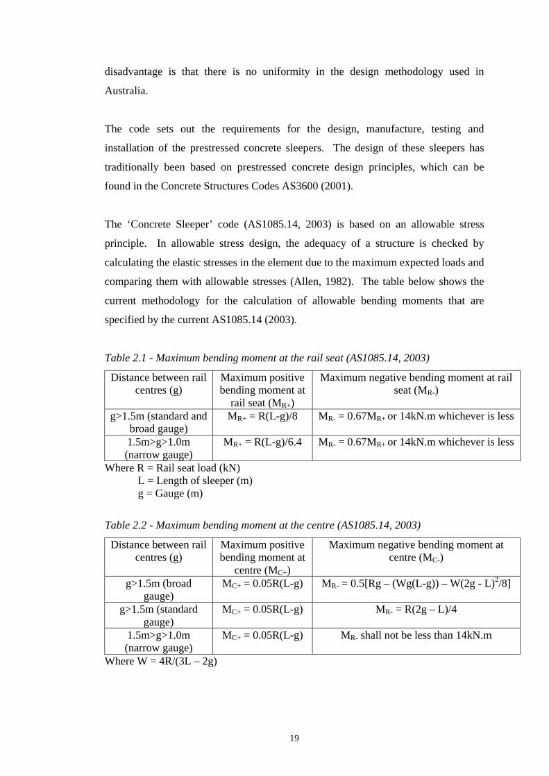
Table 2.1 Maximum bending moment at the rail seat (AS1085.14, 2003)
Table 2.2 Table 2.2 - Maximum bending moment at the centre (AS1085.14,
2003)
Table 3.1 Types of Irregularity that can be simulated (Steffens, 2005)
Table 3.2 Explanation of the Multiple Runs Window Options in Figure 3.17
Table 4.1 Benchmark I Participants
Table 4.2 Benchmark II Participants
Table 4.3 Wagon Parameters
Table 4.4 Track Components
Table 4.5 Requested Output Parameters
Table 4.6 Theories of Mechanical Behaviour used in Models
Table 4.7 Output Parameters Presented
Table 4.8 Correlation between models and Lara field data
Table 4.9 Summary of Results
Table 7.1 Proposed Wheel Maintenance Factors
Table 7.2 Possible Track Importance Factor Values
Table 7.3 Proposed Track Importance factors
Table 7.4 Braeside Track Parameters
Table 7.5 Braeside Parameters
Table 7.6 Rail Seat Bending Moment M*
xvii
Notation BOEF Beam on Elastic Foundation
DSM Discretely Supported Model
FEM Finite Element Model
DoF Degree of Freedom
Acronyms Rail CRC Cooperative Research Centre for Railway Engineering and Technologies
QR Queensland Rail
QUT Queensland University of Technology
UoW University of Wollongong
CQU Central Queensland University
CRE Centre for Railway Engineering
RC Rail Corporation (NSW)
ARTC Australian Rail Track Corporation
ARA Australasian Railways Association Inc.
ROA Railways of Australia
RSSB British, Rail Safety and Standards Board
RTRI Railway Technical Research Institute
DFG German Research Council
CHARMEC CHAlmers Railway MEChanics
AAR American Association of Railroads
TTCI Transportation Technology Center Incorporated
Computer Model Names DARTS Dynamic Analysis of Rail Track Structures
DIFF Vehicle-Track Dynamic Analysis Model
DTRACK Dynamic Analysis of Track
NUCARS™ New and Untried Car Analytic Regime Simulation
SUBTTI Subgrade Train-Track Interaction
VIA Vehicle Interacting with track Analysis model
VICT Interactions between Cars and Tracks

xviii
Statement of Originality The work contained in this thesis has not been previously submitted for a degree or diploma at any other higher education institution. To the best of my knowledge and belief, the thesis contains no material previously published or written by another person except where due reference is made Signed: ……………………………… Jeffrey Leong Date: ………………………………

xix
Acknowledgements The writer would like to thank Dr Martin Murray and Messrs John Powell, Nick Wheatley and Peter Hermann for their time, education and motivation in the completion of this research. The writer is also grateful to Queensland Rail, particularly Messrs Brian Hagaman and Ernie McCombe for the opportunity to undertake a Masters of Engineering by Research. The writer would also like to thank the Rail CRC steering committee for Project 5/23, including Messrs Karl Ikaunieks, Ric Lewtas, Steve Douglas, John Cowie and Sakdirat Kaewunruen Dr Alex Remennikov for their guidance and support. An acknowledgment also goes to Zhenqi Cai and Mr Clayton Firth for their dedication, contributions and efforts in developing the DTRACK model. The writer also wishes to recognize the contribution made by the participants of the Benchmark II Test undertaken as part of the research, including Mr David Steffens, Drs Alejandro Roda Buch, Anton Kok, Jens Nielsen, Ulf Gerstberger, Luis Baeza, Nick Wilson, Xinggao Shu and Professor Coenraad Esveld. Thanks also go to Mr Ian Telford for his brilliant knowledge, skills and assistance in spread sheeting that have helped the writer to complete his thesis. The writer also thanks the support of his family and friends who have given him their time and support during the course of his candidature.

xx
Accepted Abstracts Leong, J., Steffens, D.M. and Murray, M.H. (2006), Examination of Railway Track
Dynamic Models, International Heavy Haul Conference, 11-13 June, Kiruna,
Sweden.
Leong, J. and Murray, M.H. (2006), Probabilistic Analysis of Train/Track Impact
Forces, Journal of Engineering Mechanics, American Society of Civil Engineers.

xxi

1
CHAPTER 1
Introduction
1.1 Background of the Research
Railway track owners in Australia are under increasing commercial pressures to
extract as much performance as possible from their track asset without wholesale or
catastrophic failure. To achieve this, track owners are increasing the operational
speeds and carrying capacities of the railway track. However, there is insufficient
knowledge of the dynamic loadings that the railway track is subjected to in its
lifetime and therefore the capacity of the track is not known. In addition, there is
widespread suspicion that the railway track, particularly concrete sleepers, have
untapped reserves of strength that have potential engineering and economic
advantages for track owners.
In 1996, the Australasian Railway Association Inc (ARA) initiated a review of the
Australian Standard ‘Permanent way materials: prestressed concrete sleepers’
(Standards Australia, 2003) to address the inadequacies in knowledge of track forces
and their transmission to and below concrete sleepers. The ARA prepared a brief
which noted the need for an approach that would clarify the railway loads and their
distribution into the track for application to the various types of railway operations in
Australia such as heavy haul, freight and passenger services.
Murray and Cai (1998) initiated a comprehensive literature review on research
related to concrete sleepers as a response to the ARA brief. The report found that a

2
more cost effective appreciation of track performance could be realised with further
research, particularly with a more specific definition of the loading environment and
a better understanding of the flexural behaviour of the sleepers to impact loadings.
To address some of the issues identified by Murray and Cai (1998) a comprehensive
set of measurements of track forces of the various mix of traffic in Australia would
be needed to specify the definition of the loading environment. With a
comprehensive set of track forces data and the aid of a track analysis model, the
forces resulting from trains can be more accurately quantified and as a result railway
track owners will be able to make more efficient use of the track structure.
The need for measuring various dynamic traffic loading regimes (heavy haul, freight
and passenger) is that the risks associated with the various operations are all
different. For example, heavy haul and freight operations are based on commercial
risks whereas passenger traffic is based on safety risks. In addition, the dynamic
load profile is heavily dependent on the characteristics of the vehicle set up.
This research forms one of many research projects under the Cooperative Research
Centre for Railway Engineering and Technologies (Rail CRC). The project is titled
‘Dynamic Analysis of Track and the Assessment of its Capacity with Particular
Reference to Concrete Sleepers’. The project is a joint collaboration between the
Queensland University of Technology (QUT) and the University of Wollongong
(UoW) with the aim of developing in part a new limit state approach for the
Australian Standards AS1085.14 ‘Permanent Way Materials: Prestressed Concrete
Sleepers’ (Standards Australia, 2003).
1.2 Rail CRC Project Aim
The broad aim of this Rail CRC project is to help railway track owners to make more
cost effective use of the track asset through improved knowledge of track behaviour
under static, quasi static and dynamic loading and in particular through a more
realistic process of analysis for the design of concrete sleepers.

3
The project aims to achieve the following:-
1. Complete the development of a software package for the rigorous analysis
of dynamic behaviour of railway track in Australia;
2. Establish a probabilistic based assessment methodology for railway track;
3. Develop a more realistic design approach for Standards Australia,
‘Prestressed Concrete Sleeper Code’ (AS1085.14, 2003); and
4. Provide track owners with saving flowing from increased confidence in the
capacity of track and sleepers to carry traffic.
The research presented in this thesis will also aim to provide the Australian railway
industry and research community with a limit state design methodology for railway
track loadings so that assessment of track capacity can be undertaken with
confidence.
1.3 Scope of this Research
The scope of this research includes:
1. Review of the current Australian Standards for railway track, limit state and
present track design procedures;
2. Development of a dynamic track computer model;
3. Collection and analysis of wheel/rail impact force data; and
4. Developing a limit state methodology for railway track.
1.4 Methodology
To extract further performance out of the track asset, a more realistic assessment of
the loading scenarios is needed to determine the boundaries of track capacity. The
research presented in this thesis aims to make the assessment of railway track based

4
on more probabilistic loading scenario by establishing a limit state design
methodology for railway track.
To establish a limit state design methodology for railway track, the following would
be needed:-
1. A dynamic track model capable of simulating the track components reactions
to train loadings for future operations;
2. Validation of the model against actual track data;
3. Comprehensive set of wheel/rail impact data;
4. Establishment of probabilities and return periods for wheel impact events;
and
5. Develop a limit state methodology based on the collected data.
The outcomes of this research is to ultimately establish a limit state design
methodology for railway track that is capable of being adapted to the other types of
railway operations in Australia.
1.5 Structure of this Research
The structure of this research will be separated into the following parts:
1. Present a background on the definitions of a railway system, the current
design practices and standards for railway track;
2. Development and validation of a track dynamic computer model;
3. Measurement and analysis of wheel/rail forces; and
4. Development of a limit state design methodology for railway track.
Chapter 1 introduces the research and presents its purpose, methodology and
expected outcomes of the research.

5
Chapter 2 provides background information on the railway system including
common terminologies and definitions used in railway engineering. The chapter also
presents the methodologies used in the design of railway track as well as the
standards that govern the design of track.
Chapter 3 presents the development and updates of a dynamic track model that will
be used for this research. The chapter also provides a case study as a guide on the
models use.
Chapter 4 presents a benchmarking exercise which compares field data against the
outputs of the various participating dynamic models against the dynamic model
developed in this thesis. A discussion on the merits and disadvantages of the
developed dynamic model is also provided in this chapter as well as justification on
its suitability for this research.
Chapter 5 provides a description on the equipment that was used to collect the
wheel/rail data and how the data was processed for analysis. The chapter also
presents the collected wheel/rail force data and provides an insight on how the data
can be used to establish probabilities and return periods of impact forces.
Chapter 6 establishes a methodology to predict probabilities and return periods of
impact forces from the wheel/rail data. The chapter also investigates the influence of
varying parameters (such as changes to operational speed) that may alter the impact
force distributions.
Chapter 7 develops a limit state methodology for the design of railway track based
on the data presented in Chapter 5 and 6. The chapter also explains the implications
for railway businesses due to the standards being transformed into a limit state
principle.
Chapter 8 concludes the thesis and provides recommendation for further research that
was presented throughout this thesis.

6
CHAPTER 2
Railway Track Terminology, Design and Standards
2.1 Introduction
The design of railway is very complex due to the nature of the loadings from the
train to the railway track. Railways are traditionally separated into two systems, the
rollingstock and the railway track. This thesis will focus on the latter, however it is
very important to understand the train and track system as a whole as the two
systems are intertwined.
This chapter will present the common terminology used to discuss the railway
system and the current design methodologies used for track design. The standards
that govern the design of railway track in Australia will also be reviewed as it is
important to understand the limitations of the current standards and procedures.

7
2.2 Railway Terminology
The vocabulary used to describe railway components varies between countries and
even railway organisations. This section will explain some of the most common
terminology used in Australia and within this thesis, to provide a general background
into railways.
The railway system is generally separated into three main parts:-
1. The vehicle;
2. The wheel/rail interface; and
3. The track structure.
2.2.1 The Vehicle
Rollingstock is the typical term used to describe trains and is composed of two types
of vehicles that enable the train to operate, the locomotive or power car and the
wagons. The wagon is typically made up of a car body and two bogies as shown in
Figure 2.1.
Figure 2.1 Components of the vehicle (Popp and Schiehlen, 2003)

8
The car body is a container that carries the goods (human or material) of the train.
The car body has generally six motions of movement as shown in Figure 2.2 below.
Figure 2.2 Definitions of vehicle motions (Skerman, 2004)
The bogie is positioned under the car body and is responsible for guiding the train on
the rails. The most common type of bogie is the three piece bogie and as the name
suggests, is typically made up of three main parts; the wheelsets, sideframe and
bolster as seen in Figure 2.3.
Figure 2.3 Three piece bogie (Shabana and Sany, 2001)

9
Three piece bogies provide poor ride quality and low levels of lateral stability due to
the bogie having only secondary suspension. The Secondary Suspension group is
located between the bolster and the side frame. It should be noted that wagons with
only secondary suspension generate higher impact loadings compared with wagons
with both primary and secondary suspension due to the higher unsprung mass (Sun,
2003).
Some wagons, notably passenger trains have additional suspension know as the
primary suspension group which is located between the wheel set and the side
frames. Primary suspensions provide significant improvements to lateral stability
and ride quality, but are more expensive to maintain than bogies with only secondary
suspension. For this reason, this type of set up is mainly found on passenger wagons.
The unsprung mass of a vehicle is the mass of the components which are not
dynamically isolated from the track by suspension elements. For example, the
unsprung mass of the bogie in Figure 2.3 would consist of the wheelset and
sideframe only.
The Bolster spans between the two side frames each end resting on Secondary
Suspension, which provide vertical and some lateral flexibility. A top centre casting
on the vehicle body rests on a recessed centre plate (centre bowl) in the bolster, its
rim preventing longitudinal or lateral relative movement.
Side Frames sit directly on top of the axle boxes or package bearing adaptors and tie
the two wheelsets together longitudinally, transferring the load from the wagon to the
wheelset. The wheelset is the assembly consisting of two wheels and bearings on an
axle. Two wheelsets are fitted to bogies at each end of the vehicle, which can yaw in
order to negotiate curves.
The Wheel is the contact element connecting the vehicle to the track. Wheels are
conical rather than cylindrical in shape. This promotes a centring effect that helps the
wheel set through curves and slight lateral displacements of the track (Esveld, 2001).
The wheel also has flanges on the inside of the track to prevent derailments.

10
2.2.2 Wheel/rail Interface
The connection of the vehicle and track through the wheel-rail interface is critical for
the successful operation of trains. If the connection is interrupted through breakdown
of either system, a derailment could occur which may have significant consequences.
Figure 2.4 (a) & (b) shows how the entire train load is distributed down into the track
system through a very small contact area on each wheel.
Figure 2.4 (a) & (b) Wheel-rail contact (Knothe et al., 2001)
The Hertz theory (1887) theorises the stresses that occur at the wheel rail interface
in the vertical plane: the elastic deformation of the steel of the wheel and of the rail
creates an elliptic contact area. The dimensions of the contact ellipse are determined
by the normal force on the contact area and the hardness of the wheel and rail
running surfaces, while the ratio of the ellipse axes depends on the curvatures of the
wheel and rail profiles. The shape of the contact ellipse changes in relation to the
location of the wheel-rail contact area across the railhead. Inside the contact area, a
pressure distribution develops which in a cross section is shaped in the form of a
semi-ellipse with the highest contact pressure occurring at the centre (Esveld, 2001;
Knothe et al., 2001).

11
Defects at the wheel/rail interface (such as wheel defects and dipped joints) can
cause dynamic impact forces to occur and induce significant forces into the railway
track. This thesis will only be examining the effects of wheel defects due to the
scope of the research and time constraints. In particular flat spots on the wheel tread
can occur at random with a high probability; impact forces caused by wheel flats are
not localised effects (such as the effects of a dipped joint) and can impact randomly
along a section of railway track.
The dynamic impact loads induced into the track by rollingstock are almost entirely
due to irregularities in the roundness of the wheels (Frederick, 1978). When
designing prestressed concrete sleepers, it is important to consider the magnitude of
the forces generated by wheel irregularities, particularly wheel flats, and the
probabilities of the event occurring.
Wheel flats are defined as a chord forming on the circumference of the wheel or
simply, a flat zone on the wheel circumference. Irregularities on the tread of the
wheel generate very high dynamic forces and are the most common peak forces
encountered by the track structure in its service life. Wheel irregularities are
typically classified into three categories: out of roundness wheels, tread damage from
loss of materials, flat zones (wheel flats) on the circumference. Wheel flats are
produced by the wheels locking during braking, moving off with the brakes on and
shunting a vehicle with brakes on (Tunna, 1988). Figure 2.5 shows a classical
response of the track to a wheel flat strike.

12
Figure 2.5 Classical response to a wheel flat (Frederick, 1978)
The graph shows that as the wheel flat pivots on its leading edge, there is a period of
unloading. As the wheel/rail force drops to zero during this period of unloading, the
rail begins to rebound from its deflected shape and moves back towards the wheel,
thus attempting to separate itself from the sleeper and the ballast. A peak force is
then created (P1) due to the wheel/rail contact upon landing. Very soon after the
initial contact between the wheel/rail, a second peak is created due to the combined
wheel/rail masses impacting on the sleeper known as the P11/2 force. The third peak
(P2) is a result of the wheel/rail and sleeper masses colliding with the ballast
(Frederick, 1978).
Research undertaken by (Tunna, 1988) at British Rail defines three distinct
frequencies arising from these forces in response to wheel flat strike as:
- P1 – The wheel bouncing on the rail typically ~ 1500Hz
- P11/2 – The wheel and rail bouncing on the sleeper ~ 200Hz
- P2 – The wheel, rail and sleeper bouncing on the ballast ~ 45Hz
The effects of a freshly slid wheel flat can generate forces significant enough to
crack a concrete sleeper. However, it should be noted that these forces are not
continuously sustained. As the wheel flat eventually becomes rounded, it produces
lower frequency responses and which may reduce in magnitude at higher speeds.

13
2.2.3 The Track Structure
The typical track structure used throughout Australia is ballasted track. Other types
of track systems such as slab track are also used, however this research will be
focusing on the ballasted track structure.
The components of ballasted track structures are grouped into two main categories:
- The superstructure consisting of the rails, rail pads, sleepers, ballast and sub
ballast (capping layer); and
- The substructure consisting of the subgrade (formation) and the insitu
material.
Figure 2.6 General ballasted track configuration (Profillidis, 2000)
Rails are the longitudinal steel members that directly guide the train wheels evenly
and continuously (Sun, 2003). Rails distribute the concentrated wheel loads to the
spaced sleeper supports. The rails are held to the sleepers by fasteners and resist
vertical, lateral, longitudinal and overturning moments of the rails.
Rail pads or plates are required between the rail seat and the sleeper surface
primarily as a damper to the dynamic loads induced into the track by rolling stock
and reduction of rail-sleeper contact attrition.
Sleepers are essentially elastic beams that span across and tie the two rails together.
They have several important functions including receiving the load from the rail and

14
distributing it over the supporting ballast at an acceptable ballast pressure level,
holding the fastening system to maintain proper track gauge, and restraining the
lateral, longitudinal and vertical rail movement by anchorage of the superstructure
into the ballast. In addition, concrete sleepers provide a cant to the rails to help
develop proper rail-wheel contact by matching the inclination of the rail to the
conical wheel shape.
Ballast is the layer of crushed stone on which the sleepers rest. The ballast assists in
track stability by distributing and reducing load from the track uniformly over the
subgrade. It anchors the track in place against lateral, vertical and longitudinal
movement by way of irregular shaped ballast particles that interlock with each other.
Any moisture introduced into the system can easily drain through the ballast away
from the rails and sleepers. The coarse grained nature of ballast assists in track
maintenance operations due to its easy manipulation. The rough interlocking
particles also assist in absorbing shock from dynamic loads by having only a limited
spring-like action (Hay, 1982).
Sub ballast, also known as the capping layer is usually a broadly graded material
that assists in reducing the stress at the bottom of the ballast layer to a tolerable level
for the top of the subgrade. The sub ballast is usually an impervious material that can
prevent the inter penetration of the subgrade and ballast, thereby reducing migration
of fine material into the ballast which affects drainage. This layer also acts as a
surface to shed water away from the subgrade into drainage along the side of the
track.
Subgrade, also known the formation, is the soil that offers the final support to the
track structure. The subgrade bears and distributes the resultant load from the train
vehicle through the track structure. The subgrade facilitates drainage and provides a
smooth platform, at an established grade, on which the track structure rests.

15
2.3 Contemporary Railway Track Design
The fundamental purpose of design is to produce a structure that performs
satisfactorily and is safe from collapse. Satisfactory performance implies that the
structure under all loads and possible load combinations has limited deformations
such that the function of the structure is not impaired (Hughes, 1980).
Design requires the determination of forces that are induced into the structure, then
designing the structure to resist these forces. However, in the design of railway
track, the forces induced into the track structure are complicated due to the nature of
loading from the vehicle traversing on the track. In addition the support condition of
the railway track structure is complex due to the numerous degrees of freedoms of
motion in the track structure.
When a railway vehicle traverses the track structure, it induces forces that are
different from static forces due to the general roughness and irregularity of the track
alignment. These forces are known as Quasi-Static Forces, which are dynamic
loads that are less than 10Hz (Zhang, 2000). Due to quasi-static forces having such
low frequencies, the track structure tends to react to these loads similarly to static
loadings.
The most common procedure for calculation of the quasi static force in Australia is
the methodology presented by the Railways of Australia (ROA) manual, A Review
of Track Design Procedures (Jeffs and Tew, 1991).
The present common method to calculate quasi-static forces in railway track is to
multiply the static design load by the Dynamic Impact Factor (Jeffs and Tew,
1992). The dynamic impact factor allows the quasi-static loads to be expressed as a
multiple for the appropriate static loads (Grassie, 1992). It should be noted that this
is an empirical method and ignores vertical track elasticity, which absorbs some of
the impact forces that are induced into the rail (Jeffs and Tew, 1992).
16
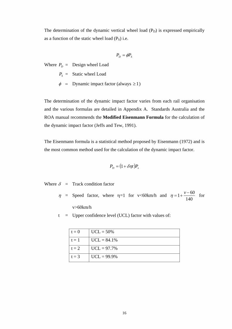
The determination of the dynamic vertical wheel load (PD) is expressed empirically
as a function of the static wheel load (PS) i.e.
SD PP φ=
Where DP = Design wheel Load
SP = Static wheel Load
φ = Dynamic impact factor (always 1≥ )
The determination of the dynamic impact factor varies from each rail organisation
and the various formulas are detailed in Appendix A. Standards Australia and the
ROA manual recommends the Modified Eisenmann Formula for the calculation of
the dynamic impact factor (Jeffs and Tew, 1991).
The Eisenmann formula is a statistical method proposed by Eisenmann (1972) and is
the most common method used for the calculation of the dynamic impact factor.
( ) sD PtP δη+= 1
Where δ = Track condition factor
η = Speed factor, where η=1 for v<60km/h and 140
601 −+=
vη for
v>60km/h
t = Upper confidence level (UCL) factor with values of:
t = 0 UCL = 50%
t = 1 UCL = 84.1%
t = 2 UCL = 97.7%
t = 3 UCL = 99.9%

17
Research and field tests undertaken by Broadley et al. (1981) have suggested the
following track condition factors for Australian conditions:
δ = 0.1 For track in “very good” condition (TCI up to 35)
δ = 0.2 For track in “good” condition (TCI up to 45)
δ = 0.3 For track in “average” condition (TCI up to 55)
δ = 0.4 For track in “poor” condition (TCI up to 70)
δ = 0.5 For track in “very poor” condition (TCI over 70)
Where TCI means Track Condition Indicies
Broadley et al. (1981) also introduced a loading factor β to account for the difference
between empty and loaded vehicles. Therefore, the Modified Eisenmann Formula
becomes:
( ) sD PtP βδη+= 1
Where, β = 1 for loaded vehicles; and
2 for unloaded vehicles.
The use of an empirical methodology to calculate the forces induced into the track is
not uncommon. There are numerous different formulas used to calculate the
dynamic impact factor and the methodology selected is dependent on the railway
organisation. A comparison of the other various impact factor formulas is presented
in Appendix A. It is apparent that some of the formulas are too simplistic, relating
only to vehicle parameters (e.g. vehicle speed and wheel diameter) (Jeffs and Tew,
1991).
It should also be noted that the empirical methodology used for railway track design
does not account for the dynamic impact forces that are generated by the defects at
the wheel/rail interface. Therefore, a more realistic dynamic analysis methodology is
required to determine the probabilities, return periods and magnitudes of impact
forces induced into the track.

18
2.4 Australian Standards for Railway Track
In Australia, Standards Australia ‘Railway Track Material, Part 14: Prestressed
Concrete Sleepers’ code (AS1085.14, 2003) is the governing standard for the design,
manufacture and testing of concrete sleepers. For the determination of the design
loads, the code presents the modified Eisenmann methodology for the calculation of
the quasi static force and provides typical values of 1.4 to 1.6 times the static wheel
load for the calculation of the quasi-static force.
To account for the wheel/rail interface irregularities, the code provides another
empirical methodology for the calculation of high frequency dynamic forces. The
code states that a minimum allowance of 150 percent of the static wheel load shall be
used. However, research undertaken by Wakui and Okuda (1999), Jenkins et al.
(1974), Frederick (1978) have proven that high frequency dynamic forces can be up
to seven times the static wheel load depending on the size of the defect and vehicle
speed.
The code states that the combined quasi-static and dynamic design load factor shall
not be less than 2.5 times the static wheel load. The code also allows the combined
quasi-static and dynamic load to be equivalent to 2.5 to 3.0 times the static wheel
load for balanced loads at speeds of 80km/h and 115 km/h respectively in the
absence of a detailed analysis (AS1085.14, 2003 Clause F4). The series does not
take into account that some trains are currently operating at speeds in excess of
115km/hr and the neglect of the standard address to such increase in speed has led to
the need to update the code to suit contemporary operating conditions and
environment.
The code also does not consider the effect the track support systems (such as the
ballast layer) have on the dynamic impact loads. The code relies on the purchaser to
approve the design of track components that are suitable for their operational
environment and conditions. The reliance on the purchaser has advantages such as
designing the concrete sleeper for their specific environment, however the
19
disadvantage is that there is no uniformity in the design methodology used in
Australia.
The code sets out the requirements for the design, manufacture, testing and
installation of the prestressed concrete sleepers. The design of these sleepers has
traditionally been based on prestressed concrete design principles, which can be
found in the Concrete Structures Codes AS3600 (2001).
The ‘Concrete Sleeper’ code (AS1085.14, 2003) is based on an allowable stress
principle. In allowable stress design, the adequacy of a structure is checked by
calculating the elastic stresses in the element due to the maximum expected loads and
comparing them with allowable stresses (Allen, 1982). The table below shows the
current methodology for the calculation of allowable bending moments that are
specified by the current AS1085.14 (2003).
Table 2.1 - Maximum bending moment at the rail seat (AS1085.14, 2003)
Distance between rail centres (g)
Maximum positive bending moment at
rail seat (MR+)
Maximum negative bending moment at rail seat (MR-)
g>1.5m (standard and broad gauge)
MR+ = R(L-g)/8 MR- = 0.67MR+ or 14kN.m whichever is less
1.5m>g>1.0m (narrow gauge)
MR+ = R(L-g)/6.4 MR- = 0.67MR+ or 14kN.m whichever is less
Where R = Rail seat load (kN) L = Length of sleeper (m) g = Gauge (m)
Table 2.2 - Maximum bending moment at the centre (AS1085.14, 2003)
Distance between rail centres (g)
Maximum positive bending moment at
centre (MC+)
Maximum negative bending moment at centre (MC-)
g>1.5m (broad gauge)
MC+ = 0.05R(L-g) MR- = 0.5[Rg – (Wg(L-g)) – W(2g - L)2/8]
g>1.5m (standard gauge)
MC+ = 0.05R(L-g) MR- = R(2g – L)/4
1.5m>g>1.0m (narrow gauge)
MC+ = 0.05R(L-g) MR- shall not be less than 14kN.m
Where W = 4R/(3L – 2g)

20
The limitations of an allowable stress design approach to designing prestressed
concrete sleepers is that it may lead to over-design of the concrete sleeper because
allowable stress assumes that there is no post steel yield capacity which is not true in
practice (Allen, 1982). Therefore, more steel maybe needed than necessary to keep
the stresses below the allowable limit.
Other limitations of an allowable stress design include (Allen, 1982):
• Probability of loads occurring;
• Level of reliability required of structural members; and
• Neglect of the material strength of concrete and steel and overlooking
requirements for serviceability such as cracking, deflection and vibration.
The limitations associated with allowable stress principle that have been identified by
Allen (1982), Ellingwood and Galamblos (1982) and Hughes (1980) have led to most
structural design codes in the Australian Standard series being transformed to limit
state principles, which will be further investigated in Chapter 7.
2.5 International Standards for Railway Track
The calculation of track forces around the world are similar to the method presented
in the ROA (Jeffs and Tew, 1991), however there are different methods for
calculating the dynamic impact factor. The methods used by each rail organisation
are diverse, though they do have common factors such as vehicle speed, varied
relationships of vehicle/track construction and maintenance. Jeffs and Tew (1991)
presents a comparison of dynamic impact factor (see Appendix A). The two most
common methods to calculate the dynamic impact factor are the AREA method and
ORE method.
The American Railway Engineering Association (AREMA, 1999) has developed a
simplistic formula in calculating the dynamic impact factor known as the AREA

21
method. AREA recommends the following method for the estimation of the dynamic
impact factor for design purposes.
Dv21.51+=φ
Where D = Wheel diameter considered.
v = Vehicle velocity (miles/hr).
The drawback of the AREA method is that considerations for wheel/rail irregularities
are neglected as well as other factors that can affect track dynamics such as
maintenance regimes and track condition. The AREA method is simplistic and the
literature review undertaken by Murray and Cai (1998) has shown that the AREA
method is conservative compared to other methodologies in calculating the dynamic
impact factor.
The Office of Research and Experiments (ORE, 1965) of the International Union of
Railways has developed an impact factor with coefficients that are based entirely on
measured track results of locomotives (Jeffs and Tew, 1991). The ORE impact
factor is determined by dimensionless coefficients.
'''1 γβαφ +++=
Where α’ = coefficient that is dependent on vehicle speed, vehicle suspension and
vertical track irregularities.
β’ = coefficient that is dependent on vehicle speed, superelevation
irregularities and location of the centre of gravity of vehicle
γ’ = coefficient that is dependent on vehicle speed, track condition, vehicle
design and maintenance conditions of locomotives.
The methods in calculating the three ORE coefficients vary between rail
organisations and are dependent on the many factors that can affect vehicle dynamics
(Jeffs and Tew, 1991).

22
Similar to the empirical design methodologies presented by Jeffs and Tew (1991),
the empirical approaches used internationally are only representations of the quasi
static force induced into the track structure. These approaches do not cover impact
forces that can create failure in the concrete sleeper, therefore a different approach is
required to accommodate the impact forces that the track will encounter during
service life.
The European Standard, prEN13230-1: Railway Applications – Track – Concrete
Sleepers and Bearers (2002), is vague in its standards of design forces for prestressed
concrete sleepers and relies mainly on the purchaser. For example, clause 4.2.1 in
prEN13230-1 (2002) states that the design load is calculated by applying a dynamic
coefficient to the static wheel load. The dynamic coefficient takes into account the
normal dynamic effects of the wheel and track irregularities. The design load value
is the responsibility of the purchaser.
The advantage of the European Standard in adopting this stance is that the purchaser
is solely responsible for the design of the track structure and should be familiar and
experienced with the operational environment that the sleeper will be designed for.
Another advantage is that different countries that are within the European Union are
able to continue using existing infrastructure and develop standards to suit their
individual operational environments. However a disadvantage of the European
Standard is that it offers no guidance or limiting conditions that must be complied
with.
North American railway track standards are based on the American Railway
Engineering and Maintenance of Way Association (AREMA) manual which provide
guidelines for recommended practice (AREMA, 1999). AREMA does not offer any
limiting factors or guidance for design and has always left the standards to be the
prerogative of the individual railways based on the nature and characteristics of their
plant and operations and the specific characteristics of the geographical region or
regions through which they operate.
There has been research undertaken in Japan that focuses on the shift away from the
conventional allowable stress design approach to a contemporary design method that

23
is based on limit state principles for prestressed concrete sleepers. Studies by Wakui
and Okuda (1999) have identified that the primary hindrance to evolving the design
methodologies used in Japan is the complex dynamic behaviour of the concrete
sleeper under impact loading of the wheels. However, the current Japanese
Prestressed Concrete Sleeper Code (JIS-E1201, 1997), is still based on allowable
stress principles.
Internationally, the standards are still based on either the allowable stress principles
or rely on the purchaser/operator to specify the dynamic forces induced in railway
track. Most standards are developed by individual rail organisations which base their
standards on previous experience and the nature of their operations and geographical
conditions. In Australia, railway track asset owners have developed standards in
addition to AS1085.14 (2003), for their individual operations and characteristics, as
described in the following section.
2.6 Other Standards for Railway Track
Railway Track Asset Owners in Australia such as Queensland Rail (QR), Rail Corp
(RC) and Australian Railway Track Corporation (ARTC) have developed standards
and specifications for their own individual rail operations. The respective standards
limit the dynamic impact forces (P2 forces) generated by wheel/rail irregularities by
specifying the allowable size of wheel/rail defects. For example, in the ARTC
Freight Vehicle Specific Interface Requirements standards (2002) in Clause 2.6 – the
P2 force shall not exceed the limits specified in Rolling Stock Units (RSU) 120,
which refers to a P2 force of 200kN.
Queensland Rail has set guidelines detailing the limits for rollingstock wheel defects,
known as the Wheel Defect Identification and Rectification (STD/0026/TEC, 2001),
which identifies and limits the size of wheel defects to control the dynamic impact
forces induced into the track. The QR standard specifies that wheel flats (refer to
chapter 5.2.1) of 50mm or multiple wheel flats of 40mm are the upper limits, above
which the wheels are considered defective.

24
Rail Corp (RC) and Australian Railway Track Corporation (ARTC) have unified
standards due to the similarities of their respective infrastructure and operations.
Similar to the standards set by QR and internationally, the RC and ARTC standards
series (TDS01, 2005) specify the maximum allowable defect sizes on both the rail
and wheel to minimise the P2 forces caused by these defects.
The standards that are set by railway organisations in Australia are maintenance
standards that are written to limit the magnitude of dynamic forces induced into the
track structure. The standards are not analytical methodologies for assessing the
magnitudes of the allowable forces induced into the track, but are there for the safety
management of the railway.
Due to the varied gauges in Australia and the many different types of operating
conditions, it became necessary to develop a national standard from an engineering
perspective to minimise the number of standards that railways must conform to.
With the introduction of third party operators and maintainers into the Australian rail
network, this necessity became more evident and rail asset owners began to develop
a Code of Practice for the Defined Interstate Rail Network.
In November 1999, the Australia Transport Council agreed to fund an Inter-
Governmental Agreement for Rail Uniformity. As a result of this agreement, the
Australian Rail Operations Unit (AROU) was established to develop and implement
a Code of Practice for the Defined Interstate Rail Network for standard gauge
railways linking the major cities in Australia. The Code of Practice (ARA, 2003)
was written in part to replace the Manual of Engineering Standards and Practices
produced by the former Railways of Australia (ROA) Committee (Jeffs and Tew,
1992).
The Australian Rail Operations Unit was later incorporated into the Australian
Railway Association (ARA) which further developed the code of practice.
Currently, the code consists of five volumes:
• Volume 1 – General Requirements and Interface Management

25
• Volume 2 – Glossary
• Volume 3 – Operations and Safe Working
• Volume 4 – Track, Civil and Electrical Infrastructure
• Volume 5 – Rollingstock
Of particular interest to the track engineer in the context of this research are Volume
4, Part 3 and Volume 5, Part 2. These parts set performance criteria for both
rollingstock and track components within the defined interstate network. These
performance criteria include guidelines on wheel and rail discontinuities such as
peaked and dipped welds and wheel flats and set force limits.
Volume 4 Part 3: Infrastructure guidelines (ARA, 2003) details the performance
criteria for various track components such as rail, sleepers and ballast. Of particular
interest are the guidelines for dipped and peaked welds. For peak or dipped new
welds, the code of practice specifies limits of 0.5mm over a 1m straight edge. For
existing track, weld limits for dips and peaks have been set to 2mm over a 1m
straight edge.
Volume 5 Part 2; Rollingstock common requirements (2002) details the performance
criteria for rollingstock design and sets limits for the forces that rolling stock may
apply to the track. The code specifies that the P2 force induced into the track shall
not exceed 230kN for freight vehicles and 295kN for locomotives. The calculation
of the P2 force uses Jenkins et al. (1974) formula for design purposes.
Volume 5, Part 2, Section 8: Rollingstock common requirements (2002), Skidded
wheels, details the limits for wheel flats. The code of practice categorises wheel flats
into five grades;
Grade 1 – A single flat with length less than 25mm.
No action required.
Grade 2 – Wheel flats between 25mm and 40mm long or multiple Grade 1
Skids.

26
Freight vehicles shall have wheels re-examined for defects. No
other action is required
No speed restriction required.
Grade 3 – Wheel flats between 40mm and 60mm long or multiple Grade 2
Skids.
Freight vehicles shall be Green Carded “for repair”.
A speed restriction of 80km/hr should be placed on any vehicle
with Grade 3 flats.
Grade 4 – Wheel flats between 60mm and 100mm long.
Wheels found with this class of defect at pre-trip inspection,
terminal, depot or repair facility shall not under any circumstances
be permitted to enter or remain in service.
If defect is discovered en-route or at a location without adequate
repair facilities, the vehicle may continue to its destination or
location with suitable repair facilities at a maximum speed of
25km/h.
Grade 5 – Wheel flats greater than 100mm long.
The vehicle shall not be moved until the tread surface defect is
adequately rectified or wheel set replaced.
These standards limit the magnitude of the P2 force induced into the track by
specifying the maximum allowable defect size at the wheel and rail interface.
However, a study undertaken by Dong et al. (1994) shows that the properties of the
rail pad can significantly affect the magnitude of the P2 force on the concrete sleeper.
The research proposed within this thesis is unique as this literature review has not
found any Australian or international railway design practices and standards that are
based on limit state principles. The standards in Australia are based on allowable
stress principles where maximum allowable limits are set to minimise the effect of
traffic over track.
The limitations of basing the standards on allowable stress principles may lead to
over design of the track materials and hence produce an uneconomical outcome in a

27
commercial environment. Therefore, a contemporary design methodology based on
limit state principles is needed to address these limitations.
2.7 Summary
The common terminology used to describe the railway system (the vehicle,
wheel/rail interface and track structure) was presented in this chapter as a
background to this thesis. This chapter also presented contemporary railway track
design methodologies in Australia and internationally and illustrated the shortfalls of
the current track design methods.
The standards that govern the design of railway track in Australia and internationally
were also reviewed in this chapter and found that the standards are still based on
allowable stress principles. Standards based on allowable stress principles are a
disadvantage to designers as the theory does not consider the ultimate strength of
materials, probabilities of loads occurring and the risks associated with failure, which
can lead to structures being over designed and hence be uneconomical. Therefore
there is a need to update the standards to one that is based on probability and risk,
hence the introduction of limit state design principles, which will be further
investigated in Chapter 7.
In addition to Australian standards, many railway organisations in Australia have
their own ‘in house’ standards which govern the maximum allowable size of defects
allowed on railway track. These standards are operational standards that are
designed to minimise the dynamic impact forces that are caused by defects at the
wheel/rail interface.
In the development of a limit state based standard a comprehensive set of wheel/rail
data is needed to enable an appropriated probabilistic methodology to be established.
In addition, a comprehensive set of wheel rail data will allow for the determination of
magnitudes of forces and load combinations so the track can be designed with a more
realistic and defensible design.

28
CHAPTER 3
Dynamic Track Simulation Model - DTRACK
3.1 Introduction
This research is the second Rail CRC Project 5/23 Master of Engineering that
follows the research undertaken by Steffens (2005). Steffens (2005) thesis focused
on the identification and development of a model for railway track dynamic
behaviour that met the criteria set by the Rail CRC as well as demonstrating potential
for further development.
For these reasons, Steffens (2005) identified the Dynamic TRACK model
(DTRACK) developed by Cai (1992) as the best model for research and development
for the Rail CRC. It should be noted that Steffens (2005) referred to DTRACK as
DARTS as Steffens (2005) was unaware that the name DARTS was already being
used by another dynamic track model developed by Esveld Consulting Services.
This chapter will examine the current updated version of DTRACK, its capabilities
and its limitations as a computer dynamic model. A case study on how to use the
DTRACK program is also presented in this chapter as the updated user friendly
interface is different to the original interface developed by Steffens (2005).

29
3.2 Modifications and Upgrades to DTRACK
The original DTRACK model was developed by Cai for his PhD thesis (1992)
“Modelling of rail track dynamics and wheel/rail interaction”. Steffens (2005)
further developed the model by building a friendly user interface onto the DTRACK
program. Since Steffens (2005), there have been further upgrades to Cai’s (1992)
DTRACK program and to Steffens (2005) user friendly interface.
3.2.1 Modifications and Upgrades to DTRACK Codes
Steffens Masters thesis (2005) identified various problems in the original DTRACK
program. Since then, the original author of DTRACK has been contracted to correct
these problems. There were three specific issues with the original DTRACK
program that were identified by Steffens (2005).
The first issue with DTRACK was found in the modelling of the quasi-static forces
applied to the track in ‘ideal’ wheel/rail contact conditions. When compared to other
dynamic models during the Benchmark I exercise (Steffens, 2005), the DTRACK
model calculated wheel/rail forces significantly lower than the other dynamic
models, which as a consequence affected the model’s estimation of the magnitudes
of forces throughout the system.
The second issue with the DTRACK model was the way DTRACK handled the
stiffness and damping properties of the rail pad. DTRACK had built-in assumptions
such as fixed maximum values for stiffness and damping values for the rail pad to
save computing time which was not necessary with more modern computers.
Another issue with the original DTRACK program is the output produced for the
sleeper pad reactions for both the concrete and timber sleeper case. The problem
occurs when a train wheel passes directly over the rail pad, DTRACK showed the
magnitude of the reaction of the rail pad dropping significantly. This behaviour was

not found in the any of the other models that participated in the Benchmark I exercise
as Figure 3.1 shows.
Figure 3.1 DTRACK’s error in modelling railpad force (Steffens, 2005)
The last problem identified by Steffens (2005) was the calculation of the sleeper
centre bending moments. The issue related to how DTRACK models the sleeper
dimensions, which greatly affects the magnitudes of the bending moment.
Upon the recommendation presented by Steffens (2005), the original author of
DTRACK (Dr. Zhenqi Cai) was contracted to correct these issues. Since the
correction of these problems, a second benchmark has been completed by the writer
to assess the capabilities of the revised DTRACK outputs. The second benchmark
compared DTRACK against the results of field data as well as outputs of other track
dynamic models and is presented in the next chapter.
30

31
3.2.2 Modifications and Upgrades to DTRACK User Friendly Interface
Steffens Masters thesis (2005) was primarily focused on developing a user friendly
interface for the DTRACK program. However, Steffens (2005) did not complete the
interface and a computer programmer in partnership with the writer completed the
user friendly interface which forms a small part of this thesis.
The new interface that was developed for the DTRACK varies significantly from the
original interface. However, it should be noted that the original structure of the input
parameters has not changed.
New features that were developed for the upgraded interface include;
• Ability to undertake multiple runs which allows the user to undertake
multiple investigations with varying parameters such as various speeds and
analysis positions;
• A library that contains the parameters used investigations, for example
properties of rail, rail pads and sleepers which can be recalled;
• The outputs of DTRACK can now be graphically displayed within the
program without having to be exported to Microsoft Excel; and
• The ability to graph the results of different investigations against each other
for easier comparisons.
Many of the upgrades to the DTRACK interface were concentrated on the menus and
graphical outputs of the model. It should be noted that the original structure of the
input and output parameters of the model had not been altered and only the user
friendly interface was changed.

32
3.3 Using DTRACK
This section examines in detail how to use the DTRACK model through the new user
friendly interface. A copy of the DTRACK program is included on a CD that is
attached to this thesis, to allow installation of DTRACK onto a computer with
Microsoft Windows XP.
3.3.1 DTRACK Interface Layout
The general layout of DTRACK is similar to Steffens’ (2005) original work. Figures
3.2 and 3.3 are reproduced from Steffens (2005) Masters Thesis and illustrate the
investigation process for using DTRACK. Figure 3.2 shows the process taken for a
new investigation, whilst the flow chart in Figure 3.3 shows the process taken for
opening an existing investigation in DTRACK.
It should be noted that the DTRACK program was intended to be used by track
engineers who possess a good understanding of the parameters that are required by
DTRACK.

33
Figure 3.2 Flow Chart for the Operation of DTRACK Interface (New investigation)
Adopted from Steffens (2005)
InvestigationMenu
DTRACK Workspace
ResultsMenu
New ... Open ...
Investigation 1
Save As…
Investigation 1 . inv
FREVIB. INF DAMP1. INF
NATVIB.OUT RESULTS . OUT
Has all Databeen collectedsuccessfully ?
Save As ...
Investigation 1 . inv
DTRACK.INP Investigation 1
Run DTRACK
Yes
AB
DTRACK Workspace
Track Data Irregularity Data Analysis Data Vehicle Data Commentary Multiple Runs
Investigation Menu
No
HelpMenu
Exit

34
Figure 3.3 Flow Chart for the Operation of DTRACK Interface (open investigation)
Adopted from Steffens (2005)
Investigation1.inv
Investigation 1
Keep Track Data ?
Save As ...
Investigation 2 .invOr
New File Name
RESULTS . OUT
DRACK Workspace
Has all Data been collected successfully ?
Save As…
Investigation2.inv Or
New File Name
Run DTRACK
FREVIB.INFDAMP1.INF
NATVIB.OUTRESULTS.OUT
DTRACK.INPInvestigation1
DTRACK.INPInvestigation2
Save As...
Investigation2.invOr
New File Name
Yes
No Yes
A
B B
Keep Track Data Checkbox
No
Investigation1:FREVIB . INFDAMP 1 . INF
NATVIB . OUTInvestigation
Menu
Track Data Irregularity Data Analysis Data Vehicle Data Commentary Multiple Runs

35
3.3.2 Undertaking an Investigation
The DTRACK program is executable through Microsoft Windows XP from a
shortcut that the installation automatically places on the desktop or from the start
menu as shown in Figure 3.4.
Figure 3.4 DTRACK Desktop Icon
When the user first enters the program, there are three menus available to the user for
selection which include (as seen in Figure 3.5):-
• Investigation menu – for creating, opening and saving investigations;
• Results menu – for examining results from simulations; and
• Help menu – for further guidance on the interface.
Figure 3.5 Menus available to user in DTRACK

36
To start an investigation, the user enters the Investigation menu where two options
are available for selection:-
1. New – Creates a new investigation where parameters have to be specified.
2. Open – Loads up an existing investigation where parameters were previously
set.
For the purposes of the following example, the ‘New’ option will be selected where
an ‘Investigation’ window will pop up allowing the user to input parameters into the
program. Figure 3.6 shows the investigation window.
Figure 3.6 Investigations Window in DTRACK

37
When the ‘Investigation’ is opened, there are six tabs at the top of the window where
the input data has to be inserted into the boxes provided. The six tabs in Figure 3.6
are input parameters for:-
• Track – rail size, gauge, rail pad type, sleeper type, sleeper spacing and track
bed type;
• Irregularity – irregularity of rail (such as dipped joints) and wheel irregularity
parameters (such as wheel flat);
• Analysis – where position along the sleeper and rail where analysis is to be
performed;
• Vehicle – vehicle speed, vehicle type, bogie type, wheel radius;
• Comments – additional information related to the investigation; and
• Multiple Runs – Allows for multiple investigations to be undertaken without
having to change all the input parameters.
The Tabs in the ‘Investigation’ window are arranged so that the parameters are
entered progressively from track structure to vehicle.
The ‘Graph’ and ‘Run TRACK’ buttons in the ‘Investigation’ window are inoperable
until all the parameters have been entered into DTRACK by the user, therefore
cannot run the model with incomplete inputs. The functions of these two buttons
will be explained further on the in this chapter.

38
Track Tab
The Track Tab sets the parameters for the so called ‘below rail’ components. Figure
3.7 shows the inputs required under this tab.
Figure 3.7 Track Tab
Inputs under the Track Tab are ordered down the screen so that track structure can be
designed from the top down. The user may use the predefined component
parameters provided from the drop down boxes or select the ‘Properties’ button on
the right of the drop down boxes to specify component parameters that are not
available in the drop down boxes.
It should be noted that some options in the drop down boxes have been permanently
installed in the ‘library’ of DTRACK. Parameters such as Australian Standards rail
sections are standard parameters which cannot be edited or deleted. The user may
wish to add or edit other parameters in the ‘Library’ which can be done through the
‘Properties’ buttons on the right of drop down boxes. When the parameters have
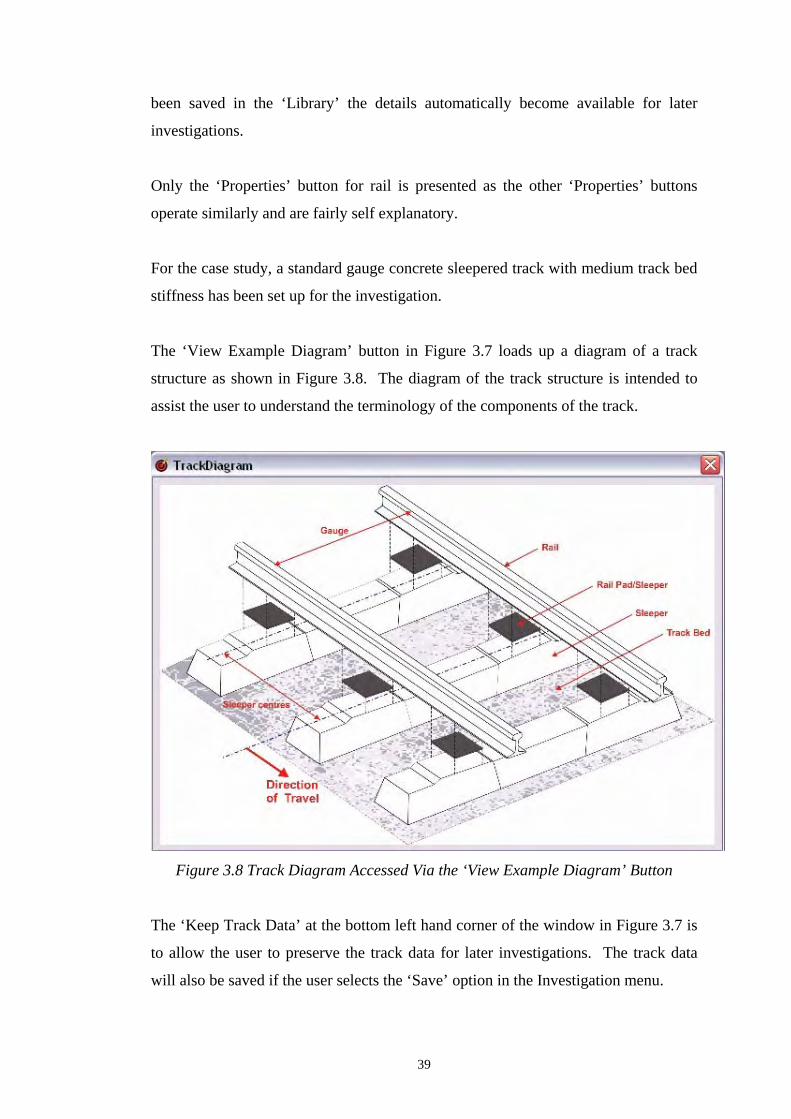
39
been saved in the ‘Library’ the details automatically become available for later
investigations.
Only the ‘Properties’ button for rail is presented as the other ‘Properties’ buttons
operate similarly and are fairly self explanatory.
For the case study, a standard gauge concrete sleepered track with medium track bed
stiffness has been set up for the investigation.
The ‘View Example Diagram’ button in Figure 3.7 loads up a diagram of a track
structure as shown in Figure 3.8. The diagram of the track structure is intended to
assist the user to understand the terminology of the components of the track.
Figure 3.8 Track Diagram Accessed Via the ‘View Example Diagram’ Button
The ‘Keep Track Data’ at the bottom left hand corner of the window in Figure 3.7 is
to allow the user to preserve the track data for later investigations. The track data
will also be saved if the user selects the ‘Save’ option in the Investigation menu.

40
Rail Properties Window
The Rail Properties Window shown in Figure 3.9 can be accessed through the
properties button on the right hand side of the rail type box near the top of Figure 3.7.
The default rail sections in this window are Australian Standards rail sections which
cannot be changed.
The user may input a non Australian Standard rail section simply by clicking the
‘Add’ button in Figure 3.9, and then specifying all the properties of the rail. The
‘Apply’ button in Figure 3.9 will only appear once all the parameters have been
input, clicking this button will also preserve the new values the user has entered.
Figure 3.9 Rail Properties Window

41
Irregularity Tab
The Irregularity Tab in Figure 3.6 allows the user to define variations in the contact
conditions at the wheel/rail interface. Upon selection of this Tab, the user can
choose from the options as shown in Figure 3.10; no irregularity assumes that there is
perfect wheel/rail interaction; the other two choices compromise irregularities at the
rail or wheel and are limited to the choices in Table 3.1 below.
Table 3.1 Types of Irregularity that can be simulated (Steffens, 2005)

42
Table 3.1 can also be viewed in DTRACK by clicking onto the ‘View Example
Diagram’ button located on the lower left hand corner in Figure 3.10.
The characteristics of these wheel or rail defects can be selected using drop down
menu boxes; the length and depth of irregularity must be specified (see Figure 3.10).
The ‘No Irregularity’ option in Figure 3.10 creates a ‘perfect’ wheel/rail contact
condition in DTRACK (i.e. perfectly round wheels and perfectly flat rail and track).
Figure 3.10 Wheel or Rail Irregularity Tab
For the case study described later, an arbitrary rail profile is used for the
investigation (refer to Chapter 4.2.4 for more details), as illustrated in Figure 3.10.
The ‘Load CSV’ button in Figure 3.10 enables the user to input a previously created
comma delimited file (*.csv) of x and y coordinates of the longitudinal rail head
profile.

43
A *.csv file of an arbitrary rail profile must have three columns in the file, with the
first column being the number of the row of data and the remaining columns are x
and y coordinates. Figure 3.11 shows the Benchmark II Arbitrary Profile 2.csv file
that is used for this case study investigation.
Figure 3.11 Example of a *.csv File for Arbitrary Rail Profile Input
A significant number of data points can be used in the arbitrary profile file. However
it should be noted that the more data points used, the longer it will take DTRACK to
process. For this case study, 548 data points were used which represented
approximately 11.1m of track.
The same process can be used to load an arbitrary wheel profile in DTRACK and the
*.csv file must be in the same format as described above.

44
Analysis Tab
The Analysis Tab in Figure 3.6 allows the user to specify the position along the rail
or sleeper at which specific output data is required (for example at the rail seat or
sleeper centre), known as the ‘analysis position’. Figure 3.12 shows the layout of the
‘Analysis’ tab. The ‘View Example Diagram’ button in Figure 3.12 is there to assist
the user to determine the analysis locations.
Figure 3.12 Analysis Tab
The drop down boxes beside the ‘Rail Analysis Position’ and the ‘Sleeper Analysis
Position’ contain predefined locations along the rail and sleeper at which DTRACK
automatically calculates output results of moments, shear etc. For each drop down
box option DTRACK calculates the coordinate of the analysis point. For the case
study, the sleeper spacing is 680mm and therefore, for the ‘MidspanBeforeSleeper’
option, DTRACK calculates the y-coordinate along the rail as -340mm as shown in
Figure 3.12. The ‘Advance Setup’ button on the lower left hand corner will be
explained in the following section.

45
Advance Setup Window
The Advance Setup button at the lower right of Figure 3.12 takes the user to a
window which allows the user to define how DTRACK is to execute the analysis.
Figure 3.13 shows the parameters that can be changed by the user in the Advance
Setup window.
Figure 3.13 Advance Setup Window
The number of sleepers and sleeper number to be analysed are fixed so that boundary
effects of the model can be minimised. The default values in this menu were based
on the recommendations of the original DTRACK author and any changes to these
parameters should only be made by an informed user.
The Time Step Analysis Setup at the bottom of Figure 3.13 group can be defined by
the user. The time step for analysis and the time step write number defines which
analysis results will be reported in the DTRACK output files. If the user has entered
the wrong values, the Default button at the bottom left hand corner of the window
can be clicked to return the values in the boxes back to the default values.
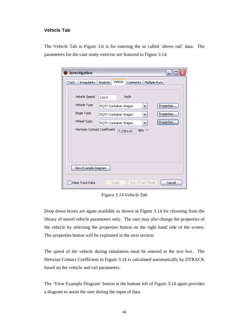
46
Vehicle Tab
The Vehicle Tab in Figure 3.6 is for entering the so called ‘above rail’ data. The
parameters for the case study exercise are featured in Figure 3.14.
Figure 3.14 Vehicle Tab
Drop down boxes are again available as shown in Figure 3.14 for choosing from the
library of stored vehicle parameters only. The user may also change the properties of
the vehicle by selecting the properties button on the right hand side of the screen.
The properties button will be explained in the next section.
The speed of the vehicle during simulation must be entered in the text box. The
Hertzian Contact Coefficient in Figure 3.14 is calculated automatically by DTRACK
based on the vehicle and rail parameters.
The ‘View Example Diagram’ button at the bottom left of Figure 3.14 again provides
a diagram to assist the user during the input of data.
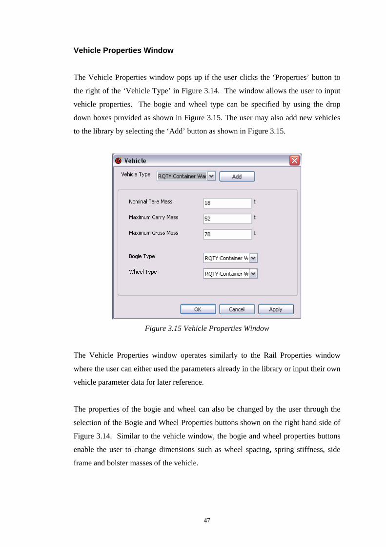
47
Vehicle Properties Window
The Vehicle Properties window pops up if the user clicks the ‘Properties’ button to
the right of the ‘Vehicle Type’ in Figure 3.14. The window allows the user to input
vehicle properties. The bogie and wheel type can be specified by using the drop
down boxes provided as shown in Figure 3.15. The user may also add new vehicles
to the library by selecting the ‘Add’ button as shown in Figure 3.15.
Figure 3.15 Vehicle Properties Window
The Vehicle Properties window operates similarly to the Rail Properties window
where the user can either used the parameters already in the library or input their own
vehicle parameter data for later reference.
The properties of the bogie and wheel can also be changed by the user through the
selection of the Bogie and Wheel Properties buttons shown on the right hand side of
Figure 3.14. Similar to the vehicle window, the bogie and wheel properties buttons
enable the user to change dimensions such as wheel spacing, spring stiffness, side
frame and bolster masses of the vehicle.
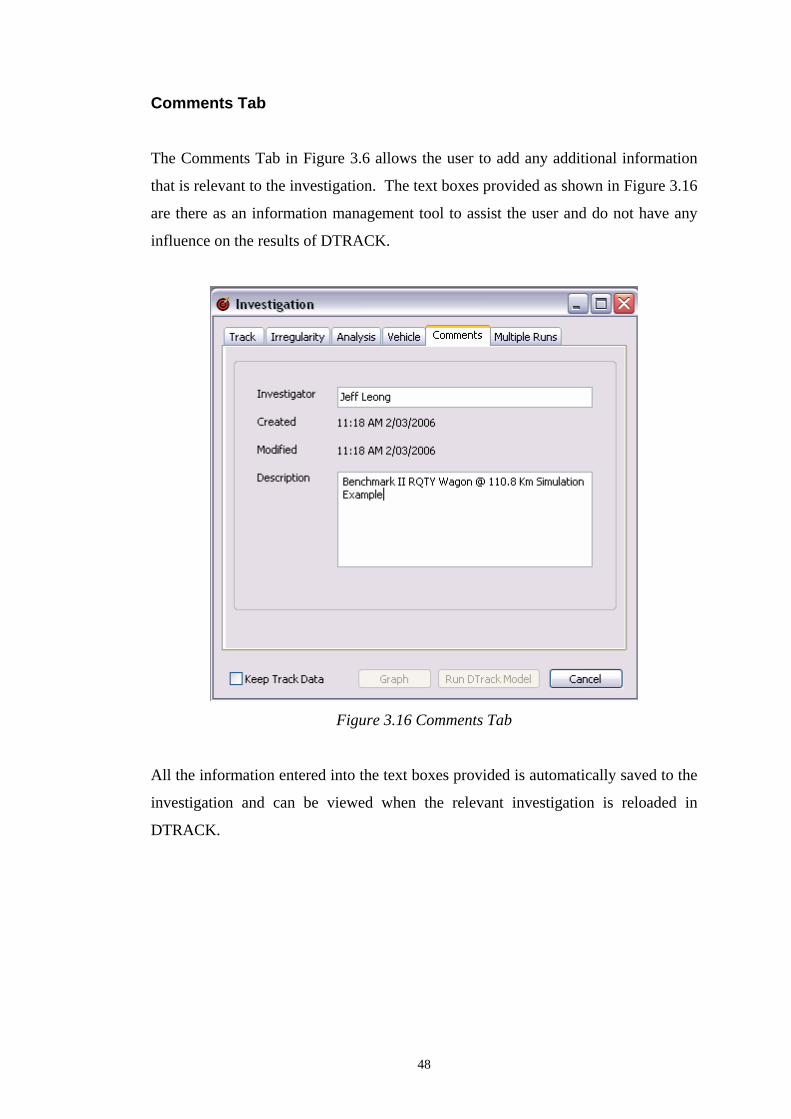
48
Comments Tab
The Comments Tab in Figure 3.6 allows the user to add any additional information
that is relevant to the investigation. The text boxes provided as shown in Figure 3.16
are there as an information management tool to assist the user and do not have any
influence on the results of DTRACK.
Figure 3.16 Comments Tab
All the information entered into the text boxes provided is automatically saved to the
investigation and can be viewed when the relevant investigation is reloaded in
DTRACK.

49
Multiple Runs Tab
The Multiple Runs Tab in Figure 3.6 enables the user to undertake multiple runs with
varying parameters without going back to the beginning of the program to re-enter all
the data from the start. Figure 3.17 shows the options available to the user in the
window accessed via the Multiple Runs tab.
Figure 3.17 Multiple Runs Tab
The Multiple Runs Tab is set up so the user can undertake multiple investigations at
various speeds (e.g. speeds at 60, 80 and 100km/hr), at various analysis positions or
with various irregularities without the need to re-enter the train and track data
repeatedly. Table 3.2 explains what each option on the Multiple Runs window
means.

50
Table 3.2 Explanation of the Multiple Runs Window Options in Figure 3.17
Option Explanation
Single Run only DTRACK will not save the data once the run is completed unless specified by the user
Vehicle Speed The user may change the speed of the vehicle
Irregularity Length The user may change the length of the irregularity on either the wheel or rail
Irregularity Depth The user may change the depth of the irregularity on either the wheel or rail
Centre of Irregularity This changes the location of the irregularity on either the wheel or rail
Rail Analysis Position This changes the position along the rail where the analysis is to take place, for example: midspan between sleepers
Sleeper Analysis Position This changes the position along the sleeper where the analysis is to take place, for example: the midspan or rail seat of the sleeper
The ‘Keep Track Data’ checkbox in Figure 3.17 also becomes available to the user
once all the data has been entered. This check box allows the user to undertake a
quicker analysis by fixing the details of the track structure. This reduces the analysis
time it takes DTRACK to run when repetitive analysis of different speeds and
analysis positions using the same track structure are to be completed.
After the investigation has been saved, the ‘Run DTRACK model’ button becomes
available as seen in Figure 3.18. Note that the name ‘Investigation’ at the top left
hand of the window has now changed to the file name the user has chosen. For the
case study, the file name in the top left of the window in Figure 3.18 has now
changed to ‘BM2 Test’.

51
Figure 3.18 Run DTRACK option becomes available when data input is completed
The program takes a few minutes to run, depending on the speed of the vehicle and
the time step setup in the ‘Advance Setup’ window the user had specified. The lower
the speed, the more iterations DTRACK will have to complete and therefore the
longer it will take to run.
Once the program has completed the simulations, the ‘Graph’ button in Figure 3.18
becomes available for graphical viewing of the results of the investigation. Clicking
on the Graph button brings up the ‘Results Setup’ window where the data can be
studied in detail.
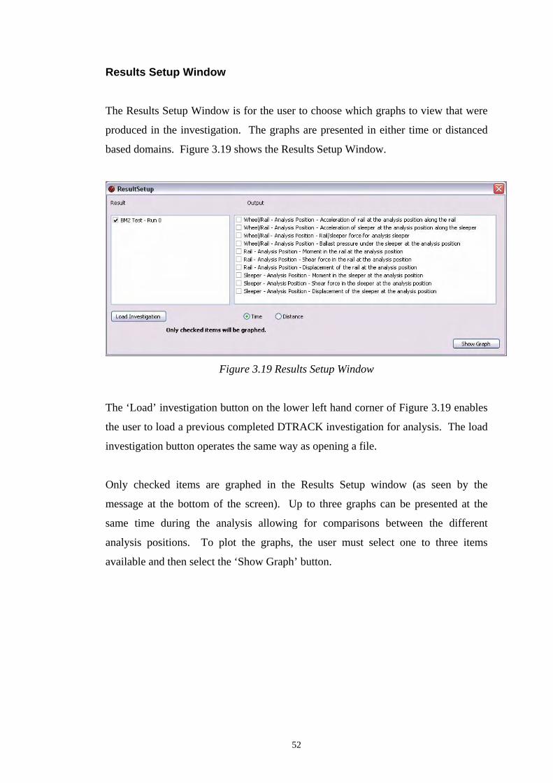
52
Results Setup Window
The Results Setup Window is for the user to choose which graphs to view that were
produced in the investigation. The graphs are presented in either time or distanced
based domains. Figure 3.19 shows the Results Setup Window.
Figure 3.19 Results Setup Window
The ‘Load’ investigation button on the lower left hand corner of Figure 3.19 enables
the user to load a previous completed DTRACK investigation for analysis. The load
investigation button operates the same way as opening a file.
Only checked items are graphed in the Results Setup window (as seen by the
message at the bottom of the screen). Up to three graphs can be presented at the
same time during the analysis allowing for comparisons between the different
analysis positions. To plot the graphs, the user must select one to three items
available and then select the ‘Show Graph’ button.

53
3.4 Summary
The DTRACK model presented in this chapter is the completed revised version of
the program that was initiated by Steffens (2005). The original author of the
program (Cai, 1992) was contracted to correct the problems with DTRACK that were
identified by Steffens (2005). In addition a programmer in partnership with the
writer completed the user friendly interface for DTRACK as part of this thesis.
Visual Basic .NET (2002) was again chosen as the programming environment to
allow for the further development to the user friendly interface. The general
Microsoft Windows interface layout structure was maintained so that the
environment was familiar to the user.
Although the general structure of the user friendly interface presented in Steffens
(2005) Masters Thesis had not changed, many of the original features have been
upgraded and improved. Improvements such as library maintenance, data
management and graphing abilities were included in the upgraded DTRACK.
A general guide and working example on undertaking a track investigation in
DTRACK was presented in this chapter. A CD of the DTRACK program is attached
to this thesis allowing for a full installation of DTRACK onto a computer with
Microsoft XP. At the time of writing of this thesis, a more detailed instructional
manual for DTRACK was being written by the author.

54
CHAPTER 4
Benchmark Tests for Models of Railway Track Dynamic Behaviour - Benchmark II
4.1 Introduction
There have been several benchmarking exercises in the past that compared the results
of various computer models of railway track. Most notable were the benchmarking
exercises of Grassie (1995), Knothe (1995) and Iwniki (1998). In each of these
benchmarking exercises, the participants were requested to provide results for
comparative analysis when provided with a set of rigorously stipulated parameters.
The overall aim of these benchmarking exercises was to validate and compare the
results of the various dynamic models against one another. However, the
benchmarking exercises did not correlate the dynamic model results against any field
data and therefore could not be an accurate indication of what occurs in practice.
The last independent benchmarking exercise was the Manchester Benchmark
undertaken by Iwniki (1998). Since that time there have been a number of more
sophisticated dynamic track models that have been developed allowing for better and
more in-depth analysis and improved representation of the railway track.

55
Steffens and Murray (2003) initiated another benchmarking exercise as a response to
the long period of time since the Manchester Benchmark which will be referred in
this thesis as Benchmark I. Benchmark I (Steffens and Murray, 2005) was very
similar to the Manchester Benchmark (Iwniki, 1998), where the same standard gauge
passenger vehicle (described in the Manchester Benchmark (Iwniki, 1998)) travelling
at 160km/hr with various wheel/rail contact defects was simulated.
The railway research organisations that participated in Benchmark I are listed in
Table 4.1.
Table 4.1 Benchmark I Participants
Model Name Research Organisations
DTRACK DynTrack Systems, USA.
DIFF CHARMEC, Sweden.
NUCARS™ Transportation Technology Center, Inc, USA.
SUBTTI Technical University of Berlin, Germany.
TRACK* Stuart Grassie Engineering Solutions, UK
VICT Southwest Jiaotong University, China * TRACK is also known as ‘Track Design v3.4’
Steffens and Murray (2005) found that the participating models had a wide range of
complexity in the theoretical basis, construction of the models and the inputs
required. In addition, Steffens and Murray (2005) also found that the outputs of
various models were dependent on the assumptions taken by the user. For example
some models required certain input parameters for their models which were not
provided in the benchmark parameters.
Benchmark I also revealed that a single set of simulations representing only one
vehicle and track scenario was insufficient to draw conclusions regarding the
behaviour of railway track as the results were not compared to field data; a further
benchmarking exercise was therefore recommended.

56
The Benchmark II exercise was therefore initiated by Steffens to compare the outputs
from the dynamic track models against field data collected at Lara, which is situated
on the Melbourne - Geelong railway line and the exercise was completed by the
writer. Another objective of Benchmark II was to continue the forum of discussion
and information that was established in the Benchmark I exercise.
The primary aim of Benchmark II was to correlate the outputs of various railway
track dynamic models against each other and against the Lara field data.
Benchmark II also provided a good opportunity to test and compare the outputs
produced by the revised DTRACK against the other models and against field data to
examine whether the results were in general agreement with the other models and the
field data. The DTRACK results used for comparison in Benchmark II would also
justify the computer models suitability for the research in this thesis as well as
establishing confidence when DTRACK is eventually released commercially.
This section will examine the input parameters of Benchmark II, the equipment used
to collect the field data, the participant’s simulation outputs for Benchmark II and a
discussion of the correlation between the various track dynamic models and Lara
field data.

57
4.2 Benchmark II Input Parameters and Instructions
Many railway research organisations from around the world were again invited to
participate in the Benchmark II exercise. The participants of the Benchmark I
exercise were also invited to participate in Benchmark II. The participants that
accepted the invitation to participate in Benchmark II are shown in Table 4.2.
Table 4.2 Benchmark II Participants
Model Name Research Organisations
DARTS Delft University of Technology, Netherlands. DIFF CHARMEC, Sweden. DTRACK DynTrack Systems, Canada & USA. NUCARS™ Transportation Technology Center, Inc, USA. SUBTTI Technical University of Berlin, Germany. VIA University of Valencia, Spain.
The outputs of the DARTS program were supplied by Delft University of
Technology (Kok, 2005).
The DTRACK model was run on behalf of its author (Cai, 2005), using the updated
version, DTRACK v2.0.
The NUCARS™ results were based on a Beta version of NUCARS™ and were
provided by Transportation Technology Centre Incorporated (TTCI) (Wilson &
Xinggao, 2005).
The DIFF, SUBTTI and VIA benchmark results were produced by their respective
authors (Nielsen, 2005; Gerstberger, 2005; Buch, 2005).
The specifications were originally developed by Steffens (2004) and sent out to the
participants. Full details of the specifications can be found in Appendix B. The
following sections briefly explain the simulation parameters and requested results for
the Benchmark II exercise.

58
4.2.1 Requested Simulations
The Benchmark II exercise was based on two freight vehicles traversing on a
concrete sleepered track structure without any wheel/rail irregularities. The
requested simulations were to be based in two dimensions only.
The selection of the simulation freight vehicles was based on two factors. The first
factor was that most railway organisations around the world operated freight traffic
travelling on concrete sleepered ballasted track. The second factor was that
Benchmark I had already simulated a passenger vehicle and therefore a freight
vehicle will allow for more definitive comparisons between the benchmarked
models.
Although no irregularities at the wheel/rail interface (such as wheel flats or dipped
joints) were simulated for Benchmark II, participants were provided with the actual
longitudinal rail head profile for their simulations which can be found in Figure 4.3.
A total of eight runs were requested from the participants:
Simulations 1 to 4: No Irregularity
Simulations 5 to 8: Actual Profile (Geelong to Melbourne)
As mentioned earlier, the participants were supplied with a comprehensive set of
input parameters which will be detailed in further sections of this chapter.
The analysis was to be undertaken around ‘Sleeper C’, where the location of ‘Sleeper
C’ was up to the discretion of the participant. Similar to Benchmark I, the
participants were asked to position ‘Sleeper C’ in a location that would eliminate any
boundary effects their model might experience. Other suggestions that were
provided to the participants included:
• Minimum total run distance of vehicle of 20m;
• Minimum time step of 0.0001 seconds (0.1 milliseconds);
• No contact filtering at wheel/rail interface.

59
4.2.2 Vehicle Parameters
The freight vehicles selected for the Benchmark II exercise consisted primarily of
two bogies with only secondary suspension. The freight vehicles selected for
Benchmark II were:
Standard Gauge – Container Wagon (RQTY Class)
Standard Gauge – Structural Wagon (RKWF Class)
Table 4.3 provides further details on the wagons speed, load and direction of travel.
Table 4.3 Wagon Parameters Sim No. Wagon Gross
Vehicle Mass Speed Destination
1 & 5 RQTY Container 52,000 kg 101.7 km/h Geelong
2 & 6 RQTY Container 78, 000 kg 110.8 km/h Melbourne
3 & 7 RKWF Structural 28,000 kg 75.0 km/h Geelong
4 & 8 RKWF Structural 100,000 kg 83.1 km/h Melbourne
The Benchmark II participants were supplied with the details of the wagons (see
Appendix B) which included the suspension characteristics, dimensions of the
vehicle body and wheel profile contact conditions. The participants were also
supplied with a detailed drawing of the bogies used by both freight wagons. The
wheels on the wagons were assumed to be free of any wheel surface defects.

60
4.2.3 Lara Test Site
The Lara test site is situated along the Melbourne – Geelong standard gauge
(1435mm) railway line in Victoria, Australia.
The instrumentation at Lara is managed by the Institute of Railway Technologies
(IRT) and the details of the Lara field set up can be found in Appendix B.
Accelerometers and strain gauges were applied to the sleepers and rails at various
locations.
The sleeper used for analysis (Sleeper C) was fully instrumented with strain gauges
and accelerometers so that the full response of the sleeper to a passing train could be
monitored. Figure 4.1 depicts the layout of the field instrumentation at Lara.
Figure 4.1 Lara Test Site, Melbourne to Geelong Track Line, Victoria
The calibration factors used for the strain gauges and accelerometers were supplied
by IRT to convert the ‘raw data’ which had been measured in millivolts (mV).
Details of the calibration factors can be found in Appendix C.

61
4.2.4 Track Parameters
The railway track at Lara is constructed with AS60 kg/m rail on concrete sleepers
resting on ballast. A capping layer consisting of road base material was also
constructed under the ballast.
At the time of data collection, the ballast was in good condition and the drainage
within the vicinity of the data collection equipment was excellent. The visual
inspection of the site yielded no defects in the ballast or subgrade within the
immediate area of the test sleeper.
No defects (such as squats or rolling contact fatigue) were detected on the rails’
running surfaces. The track is plain line track with no indication of any cross cant
issues, as recorded by the track recording car.
Figure 4.2 Typical example of a cross section of railway track at Lara.
Table 4.4 provides a general detail of the components that the track was constructed
with. More detailed information for the track structure can be found in the
Benchmark II instructions in Appendix B.
Subballast (Capping Layer)
Ballast
Formation (Subgrade)
Rails, Fasteners & Pads Sleeper Gauge 1435 mm

62
Table 4.4 Track Components Component Description
Gauge 1435mm (1505mm rail centres)
Rail AS 60kg/m
Fastener Pandrol ‘e’ clip
Rail Pad 7.5mm HDPE (No. 651840) Insulating Biscuits (No. 55088)
Sleeper Concrete (30 tonne axle load rated) with 680mm spacings
Ballast 200mm (below the sleeper base) (53mm Basaltic Rock)
Subballast 150mm (Crushed rock/scoria)
Formation Medium Stiffness
The participants of Benchmark II were supplied with the longitudinal track profile
collected with the Corrugation Analysis Trolley (CAT) (Grassie, 2004).
Approximately 11m section of rail longitudinal profile over Sleeper C was selected
and it was assumed that both rails were symmetric in profile.
The participants were required to use Profile 1 (Figure 4.3 (a)) for Simulation 6 and
8, whilst Profile 2 (Figure 4.3 (b)) was to be used for Simulation 5 and 7.
-4
-3
-2
-1
0
1
2
3
4
5
-0.16 0.52 1.2 1.88 2.56 3.24 3.92 4.6 5.28 5.96 6.64 7.32 8 8.68 9.36 10.04 10.72
(m)
(mm
)
Geelong Melbourne
Figure 4.3 (a) Profile 1 – To Melbourne (UP Direction)
Slee
per C

63
-4
-3
-2
-1
0
1
2
3
4
5
-0.46 0.22 0.9 1.58 2.26 2.94 3.62 4.3 4.98 5.66 6.34 7.02 7.7 8.38 9.06 9.74 10.42 11.1
(m)
(mm
)
GeelongMelbourne
Figure 4.3 (b) Profile 2 – To Geelong (DOWN Direction)
The location of the instrumented Sleeper C was located at 5.28m for Profile 1 and
5.66m for Profile 2. As mentioned previously, the train wheels were assumed to
have no irregularities.
4.2.5 Wheel/Rail Properties
As mentioned previously, approximately 11m of rail longitudinal profile was
recorded over the instrumented sleeper (Sleeper C) using the Rail Corrugation
Analysis Trolley known as the ‘Rail CAT’ (Grassie, 2004).
The participants were requested to assume the wheel was free of any surface defect
and was perfectly round.
4.2.6 Requested Simulation Outputs
Participants were requested to provide a number of simulations for comprehensive
comparisons against the other participants’ models and against the field data. Table
4.5 details the simulations and output that were requested of the participants.
Slee
per C

64
Table 4.5 Requested Output Parameters Code Output Parameter Unit
A Normal contact force between the wheels and rail kN
B Shear force in the rail at mid span before sleeper C kN
C Vertical acceleration of the rail at the mid span before sleeper C m/s2
D Vertical acceleration at the end of sleeper C m/s2
E Vertical acceleration at the mid span of sleeper C m/s2
F Bending moment at the rail seat of sleeper C kNm
G Bending moment at the mid span of sleeper C kNm
4.2.7 Vehicle Submodels
All the models with the exception of the NUCARSTM model represented the vehicle
with a single bogie with two wheel masses and a sideframe mass, including a
primary suspension element but no secondary suspension elements.
NUCARSTM was the only model that represented the vehicle with two bogies,
including primary and secondary suspension elements.
All six models either assumed or adopted symmetry of loading about the track centre
line. All components in all vehicle submodels were represented as rigid bodies with
linear suspension elements.
4.2.8 Wheel/Rail Interface Submodels
NUCARSTM uses a ‘Real Time Wheel Rail’ contact model that was developed in
house at TTCI. This feature allows for the actual wheel/rail contact geometry to be
computed at each integration time step continuously during the simulation. The local
deformation at the contact point of rail and wheel takes account of the contact
geometry and contact forces.

65
The remaining models are time domain models and allow non-linear Hertzian contact
conditions. The ‘lift off’ of the wheel from the rail is modelled by setting the tension
stiffness of the wheel/rail contact according to Hertz Theory to zero. The wheel/rail
contact in these models is represented by a single point and no filtering was
undertaken to allow for consideration of the actual shape of the contact patch.
4.2.9 Track Submodels
The models that participated in Benchmark II were based on different theories of
mechanical behaviour for the different components that made up the track structure.
Table 4.6 provides brief details on the theories of mechanical behaviour that were
used by each model.
Table 4.6 Theories of Mechanical Behaviour used in Models Models Element
DARTS DIFF DTRACK NUCARS SUBTTI VIA
Boundary Conditions
Fixed at rail ends
Fixed at rail ends
Fixed at rail ends
Fixed at rail ends
‘Ring” Fixed at rail ends
Rail Timo* Timo Timo Euler Timo Timo Rail Pad 1 Spring
1 Damper 1 Spring
1 Damper 1 Spring
1 Damper 1 Spring
1 Damper 1 Spring
1 Damper 1 Spring
1 Damper Sleeper Timo Timo Timo Euler Timo Timo Ballast Winkler Subballast Timo Subgrade Winkler
Winkler Winkler Winkler Half Space Winkler
*Timo = Timoshenko Beam
All the with the exception of SUBTTI assumed fixed end boundaries of the simulated
portion of track. SUBTTI uses a ‘Ring’ type model that allows for the model to
represent the track as a continuous loop simulating an infinite length.

66
4.3 Benchmark II Results
The Benchmark II results supplied by the participants are graphically presented in
this section and were processed through Microsoft Excel. Commentaries associated
with the results are also provided in this section.
4.3.1 Output Parameters
Although seven simulations were requested of the participants, only Simulations 1
and 5 (‘ideal’ versus ‘arbitrary’ wheel/rail conditions) will be analysed in this section
to demonstrate the process applied to all the simulations.
The output parameters that will be examined here are found in Table 4.7. The results
of the remaining simulations can be found in Appendix C.
Table 4.7 Output Parameters Presented Code Output Parameter Unit
A Normal contact force between the wheels and rail kN
B Shear force in the rail at mid span before sleeper C kN
C Vertical acceleration of the rail at the midspan before sleeper C m/s2
F Bending moment at the rail seat of sleeper C kNm
G Bending moment at the mid span of sleeper C kNm
4.3.2 Normal Contact Force Between Wheel/Rail
The two graphs in Figure 4.4 illustrate the differences between the models’ outputs
of the wheel/rail contact forces for (a) ‘ideal’ and (b) arbitrary longitudinal rail
profiles allowing for a detailed comparison. As can be seen, there is no consensus
amongst the models for either case.

67
1A - Normal Contact Force Between Wheel and Rail
40
50
60
70
80
90
0.300 0.330 0.360 0.390 0.420 0.450 0.480 0.510 0.540 0.570 0.600 0.630
Time (s)
Con
tact
For
ce (k
N)
DARTSDIFFDTRACKNUCARSSUBTTIVIA
Sleeper C
Figure 4.4 (a) Wheel/Rail Contact Force for Leading Wheel ‘Ideal’ Rail
Longitudinal Profile
5A - Normal Contact Force Between Wheel and Rail
0
10
20
30
40
50
60
70
80
90
100
110
0.260 0.290 0.320 0.350 0.380 0.410 0.440 0.470 0.500 0.530 0.560 0.590 0.620 0.650
Time (s)
Con
tact
For
ce (k
N)
-5
0
5
10
15
20
25
30
35
40
45
Dep
th (m
m)
DARTSDIFFDTRACKNUCARSSUBTTIVIAProfile 2, To Geelong
Sleeper C
Figure 4.4 (b) Wheel/Rail Contact Force for Leading Wheel for Arbitrary Rail Longitudinal Profile
In Figure 4.4 (a) the SUBTTI model showed the largest changes in magnitudes for
contact force for both the ‘ideal’ and arbitrary longitudinal rail profile. It is
questionable whether the results of SUBTTI would be reliable given that the peak to
peak variation of its wheel/rail contact force in Figure 4.4(a) is much larger than
would be expected by experienced rail engineers.

68
As mentioned earlier, the NUCARSTM model is capable of varying the geometry of
the contact patch. The results in Figure 4.4 show that this built-in feature of
NUCARSTM still produces results that are not too different to most of the other
models which do not possess this ability. This finding reinforces the statement made
by Grassie (1996) questioning the value of developing models with increasing
complexity as the unknowns in the systems and inherent variability of track may
overwhelm such complexities and hence not produce meaningful results.
Unlike in Benchmark I (Steffens 2005) where DTRACK’s wheel/rail contact force
was significantly lower than the other benchmarked models, the revised version of
DTRACK produced results that were very comparable to the other models as seen by
the graphs in Figure 4.4.
The DARTS and VIA models produced results that were similar to each other when
the peak to peak values were compared for the ‘perfect’ track case in Figure 4.4 (a).
However the phases of the DARTS and VIA models were out of phase with one
another as seen in Figure 4.4 (a)
There would be consequences to the user of any of the models, seeing there is such
variability in the estimation of the magnitudes of wheel/rail contact force. A major
consequence would be uncertainty in the determination of rail head stresses, rolling
contact fatigue growth and grinding maintenance estimation. Engineering decisions
would therefore be very difficult due to the level of variability in output of the
models.

69
4.3.3 Shear Force in Rail at Midspan
The graphs in Figure 4.5 (a) and (b) show the shear force in the rail for the ‘ideal’
and arbitrary longitudinal rail profiles respectively.
1B - Shear Force in Rail at Midspan Before Sleeper C
-40
-30
-20
-10
0
10
20
30
40
0.360 0.390 0.420 0.450 0.480 0.510 0.540 0.570 0.600
Time (s)
Shea
r For
ce (k
N) DARTS
DIFFDTRACKNUCARSSUBTTIVIA
Sleeper C
Figure 4.5 (a) Shear Force in Rail for ‘Ideal’ Rail Longitudinal Profile
5B - Shear Force in Rail at Midspan Before Sleeper C
-60
-50
-40
-30
-20
-10
0
10
20
30
40
50
60
0.380 0.410 0.440 0.470 0.500 0.530 0.560 0.590
Time (s)
Shea
r For
ce (k
N) DARTS
DIFFDTRACKNUCARSSUBTTIVIALARA Field Data
Sleeper C
Figure 4.5 (b) Shear Force in Rail for Arbitrary Rail Longitudinal Profile

70
It should be noted that the shear force of the field data in Figure 4 (b) is not a
representation of the shear force but a measure of the wheel/rail force, so its
maximum value should be equal to the peak-peak change in shear force of the
models.
From the graphs in Figure 4.5 it is clear that there are issues with DTRACK in the
shape and magnitude of the shear force trace and there was no clear explanation for
the reasoning behind this odd behaviour in DTRACK.
The original author (Cai) was contacted about the matter and a further revision of
DTRACK should have this problem corrected. Although the shear force in the rail
has some importance, it is not a critical parameter that would be investigated when
analysing track.
The NUCARSTM models simulation in Figure 4.5 shows that the model produced the
largest magnitudes of the shear force in the rail for both the ideal and actual
longitudinal rail profiles. Of particular interest is the comparison between
NUCARSTM and the Lara field data in Figure 4.5 (b). NUCARSTM produced a result
that was almost double of the results of Lara and was also significantly higher than
the results of the other models (such as DARTS and VIA).
The DARTS, DIFF, SUBTTI and VIA models produced shear forces that were
similar to each other for both the ideal and actual rail longitudinal profiles. When
compared to the Lara field data in Figure 4.5 (b), the peak to peak shear force result
of these models was almost equivalent with the maximum force of the Lara result.

71
4.3.4 Vertical Acceleration of the Rail at Midspan
Figure 4.6 (a) and (b) show the vertical acceleration of the rail at midspan before
Sleeper C for the ‘ideal’ and arbitrary profiles respectively. Figure 4.6 (b) also
compares the models’ outputs against the Lara field data.
1C - Acceleration of Rail at Midspan Before Sleeper C
-40
-30
-20
-10
0
10
20
30
40
0.450 0.455 0.460 0.465 0.470 0.475 0.480 0.485
Time (s)
Acc
eler
atio
n (m
/s2 )
DARTSDIFFDTRACKNUCARSSUBTTIVIA
Sleeper C
Figure 4.6 (a) Vertical Acceleration of the Rail at Midspan before Sleeper C for
‘Ideal’ Longitudinal Rail Profile
5C - Acceleration of Rail at Midspan Before Sleeper C
-500
-400
-300
-200
-100
0
100
200
300
400
500
0.440 0.450 0.460 0.470 0.480 0.490 0.500
Time (s)
Acc
eler
atio
n (m
/s2 ) DARTS
DIFFDTRACKNUCARSSUBTTIVIALARA Field Data
Sleeper C
Figure 4.6 (b) Vertical Acceleration of the Rail at Midspan before Sleeper C for
Arbitrary Longitudinal Rail Profile

72
The two graphs in Figure 4.6 clearly show that there is enormous disparity amongst
the results with each of the models having different outputs for the magnitudes and
phases of the rail acceleration.
The results produced by the SUBTTI model for the ideal longitudinal rail profile in
Figure 4.6 (a) show the most interesting accelerations when compared to the other
models outputs. The SUBTTI results in Figure 4.4 (a) show extremely large and
variable magnitudes for the acceleration of the rail. The author of SUBTTI
(Gertsberger) was made aware of the problems associated with the SUBTTI results,
however no responses from the author were received by the writer regarding the
results.
The DARTS results for rail acceleration for both the ideal and actual rail longitudinal
profile cases in Figure 4.6 show very little changes in acceleration. The results of
DARTS for the actual rail profile scenarios in Figure 4.6 (b) is not seen in the results
of the other models and therefore a good comparison with the results of Lara and the
other models could not be made.
If the peak magnitudes of accelerations within the Lara data were compared to the
peak magnitudes of accelerations of the DIFF, DTRACK, NUCARSTM, SUBTTI and
VIA model outputs in Figure 4.6 (b) a correlation between the Lara and models
results can be made which shows that the models can still be very reliable in the
calculation of rail accelerations.
The acceleration of the rail is the only acceleration parameter in Benchmark II that is
shown in this chapter. The results of the other acceleration parameters can be found
in Appendix D.

73
4.3.5 Bending Moment at the Rail Seat of Sleeper
Figure 4.7 (a) and (b) presents the bending moment of the rail seat for both the
‘ideal’ and arbitrary rail longitudinal profiles.
1F - Bending Moment at Rail Seat of Sleeper C
-3.0
-2.0
-1.0
0.0
1.0
2.0
3.0
4.0
5.0
6.0
0.350 0.380 0.410 0.440 0.470 0.500 0.530 0.560 0.590 0.620 0.650
Time (s)
Ben
ding
Mom
ent (
kNm
)
DARTSDIFFDTRACKNUCARSSUBTTIVIA
Sleeper C
Figure 4.7 (a) Sleeper Bending Moment at Rail Seat for ‘Ideal’ Longitudinal Rail
Profile
5F - Bending Moment at Rail Seat of Sleeper C
-2.0
-1.0
0.0
1.0
2.0
3.0
4.0
5.0
6.0
7.0
0.350 0.380 0.410 0.440 0.470 0.500 0.530 0.560 0.590 0.620 0.650
Time (s)
Ben
ding
Mom
ent (
kNm
)
DARTSDIFFDTRACKNUCARSSUBTTIVIALARA Field Data
Sleeper C
Figure 4.7 (b) Sleeper Bending Moment at Rail Seat for Arbitrary Longitudinal Rail
Profile

74
It should be noted that the original results supplied by Delft University of
Technology for DARTS originally contained a time shift error in the simulation of
the bending moment of the rail seat. The authors of DARTS (Esveld and Kok) were
notified of the error and informed the writer that the error was being corrected at the
time of writing the thesis. Therefore the original DARTS results with the time shift
error was not presented and instead, the time has been shifted by the writer to be in
alignment with the other results for uniformity.
The NUCARSTM model produced the largest magnitude of the sleeper moment for
the two different cases of longitudinal rail profile. When compared to the results of
the other models, NUCARSTM was quite excessive in the estimation of bending
moment at the sleeper rail seat, for example in Figure 4.7 (a) DARTS and VIA
produced a bending moment of approximately 2kN.m whilst NUCARSTM was over
4kN.m which is double that of DARTS and VIA.
The SUBTTI model produced interesting bending moment plots. The SUBTTI plots
for rail seat bending moment in both rail profile scenarios showed a small amount of
sleeper vibration of approximately 60Hz in the results, which was also evident in the
results of DTRACK.
DTRACK produced a bending moment magnitude that was comparable with the
other models and in Figure 4.7; however the profile of the bending moment is of
concern as there are a number of large peaks and dips in the bending moment profile.
This bending moment profile was not seen in the results of the other models and the
author (Cai) has been notified of the problems.
The Lara field data is presented in Figure 4.7 (b) is for information, but is not
necessarily a measure of the actual bending moment of the rail seat, as the actual
location of the strain gauge on the sleeper could not be determined from the
information supplied by the Railway Technical Institute (company responsible for
maintaining equipment at Lara); an accurate determination of the bending moment
could not be undertaken.
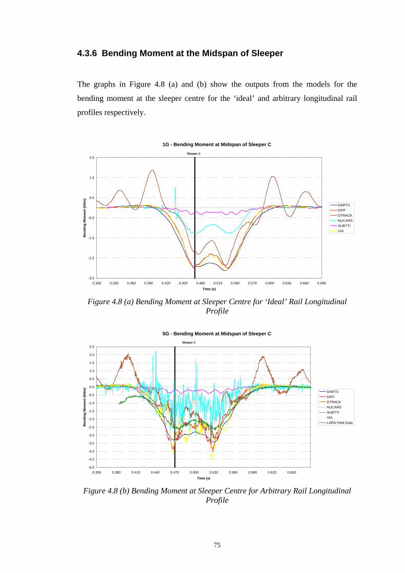
75
4.3.6 Bending Moment at the Midspan of Sleeper
The graphs in Figure 4.8 (a) and (b) show the outputs from the models for the
bending moment at the sleeper centre for the ‘ideal’ and arbitrary longitudinal rail
profiles respectively.
1G - Bending Moment at Midspan of Sleeper C
-3.5
-2.5
-1.5
-0.5
0.5
1.5
2.5
0.300 0.330 0.360 0.390 0.420 0.450 0.480 0.510 0.540 0.570 0.600 0.630 0.660 0.690
Time (s)
Ben
ding
Mom
ent (
kNm
)
DARTSDIFFDTRACKNUCARSSUBTTIVIA
Sleeper C
Figure 4.8 (a) Bending Moment at Sleeper Centre for ‘Ideal’ Rail Longitudinal
Profile
5G - Bending Moment at Midspan of Sleeper C
-5.0
-4.5
-4.0
-3.5
-3.0
-2.5
-2.0
-1.5
-1.0
-0.5
0.0
0.5
1.0
1.5
2.0
2.5
0.350 0.380 0.410 0.440 0.470 0.500 0.530 0.560 0.590 0.620 0.650
Time (s)
Ben
ding
Mom
ent (
kNm
)
DARTSDIFFDTRACKNUCARSSUBTTIVIALARA Field Data
Sleeper C
Figure 4.8 (b) Bending Moment at Sleeper Centre for Arbitrary Rail Longitudinal
Profile
76
The Lara field data presented in the graph in Figure 4.8 (b) is the actual bending
moment of the sleeper centre. Unlike the rail seat bending moment presented in
Section 4.3.5 Figure 4.7 (b) the location of the strain gauge at the sleeper centre was
known precisely and therefore an accurate calculation of the bending moment could
be made.
The SUBTTI results for the sleeper centre bending moment are the most striking for
both rail profile scenarios in Figure 4.8, in that the model produced by far the
smallest magnitudes for sleeper centre moment.
NUCARSTM produced a very curious result for the sleeper centre bending moment.
The results of the NUCARSTM model in Figure 4.8 (b) are associated with a lot of
‘noise’ which was not seen in the rail seat bending moment results in Figure 4.7 (b).
No explanation was supplied from TTCI for these results and no clear explanation
could be derived by the writer. Furthermore, the mean peak magnitude of the
NUCARSTM data for the sleeper centre bending moment was significantly smaller
than the mean peak moment of most of the other models (except SUBTTI) and the
Lara field data.
A good agreement between the DTRACK model and the field data can be seen in
that the mean peak moments are approximate to those of the Lara field data. As with
the results for the bending moment at the midspan of the sleeper, there are many
peaks and dips associated bending moment profile and the author (Cai) again was
notified of the problem.
The results produced by the DARTS, DIFF and VIA were approximate to one
another in the calculation of the mean peak magnitudes for the sleeper centre bending
moment as seen in Figure 4.8. When the results of DARTS, DIFF and VIA were
compared to the Lara field data in Figure 4.8 (a) the models were conservative in the
estimation of the magnitude of sleeper centre bending moment.

77
4.4 Summary
Benchmark II compared a number of international track dynamic models outputs
against each other and against field data collected at Lara on the Melbourne to
Geelong standard gauge railway track in Australia. Benchmark II also provided a
good opportunity to test and compare the outputs produced by the revised DTRACK
against the other models and against field data.
Within the Benchmark II exercise described in this chapter, the outputs of six models
were examined. All the models simulated track and train operating conditions that
were spelled out in a common specification.
The DARTS model is available for purchase through Esveld Consulting Services
without ongoing technical support. Benchmark II has shown that the results
produced by DARTS are very approximate to the field data and to the outputs of
most of the remaining models in terms of force magnitudes. Although DARTS had
some issues relating to the time domain for the bending moment parameter, the error
was being fixed by the authors (Esveld and Kok) of DARTS at the time of writing.
Benchmark II has shown that the results of the DIFF model was also very
approximate to the results of the other dynamic models and the field data for specific
parameters in the Benchmark II exercise. However, for the bending moments of the
sleeper, DIFF consistently produced results that were conservative in peak
magnitudes when compared to the field data and other models.
The DTRACK model will soon be available for commercial release. The DTRACK
model’s results showed that the maximum values within the results are relatively
consistant with the field data and other track dynamic models. However, Benchmark
II has shown the DTRACK has a few issues with the outputs of the model such as the
shear force in the rail and many peaks and dips in the magnitudes of the bending
moment of the sleeper. The author of DTRACK has been notified of the problems
and was addressing them at the time of writing.

78
The NUCARSTM model that was used for the Benchmark II exercise was a beta
version that is not yet available commercially. NUCARSTM was by far the most
complex of the dynamic models that participated in Benchmark II and produced
certain results that were questionable such as the shear force of the rail in Figure 4.5
(b) and the sleeper centre bending moment in Figure 4.8 (b).
The results of SUBTTI were highly variable compared to the Lara field data and the
other models, especially in the wheel/rail contact force in Figure 4.4 (a), acceleration
of rail in Figure 4.6 (a) and the sleeper centre bending moment in Figure 4.8. The
variability within the SUBTTI results in Benchmark II raises questions about the
reliability of the SUBTTI model.
The VIA model produced results that were consistently in approximation with the
field data and the other models for all the specified output parameters in Benchmark
II.
Table 4.8 summarises the Benchmark II’s participant models correlation with each
other and the Lara field data. The table is intended to provide a general overview
each models correlation with one another.
Table 4.8 Correlation between models and Lara field data DARTS DIFF DTRACK NUCARS SUBTTI VIA LARA
DARTS
DIFF
DTRACK
NUCARS
SUBTTI
VIA
= if at least 2 of the presented output parameters of one model were within 10% of the other models = if 3 or more of the presented output parameters of one model were within 10% of the other models
= if 2 or more of the presented output parameters of the model were more than 10% different from the other models

79
Table 4.9 Summary of Results
Peak Value of Output Parameter L
ara
DA
RT
S
DIF
F
DT
RA
CK
NU
CA
RS
SUB
TT
I
VIA
Average wheel/rail contact force (kN)
- 65.05 63.76 63.75 63.82 62.56 63.70
Shear Force (kN) 77.02* -10.55*
30.87 -24.65
29.95 -38.73
16.65 -17.65
50.68 -47.88
18.56 -42.76
28.49 -36.21
Average rail midspan acceleration (m2/s)
379.42 -391.13
13.55 -17.96
268.78 -179.55
172.44 -196.13
246.97 -292.23
412.88 -285.54
377.51 -574.29
Bending moment at midspan of sleeper (kN.m)
0.05 -2.82
0.14 -3.43
0.18 -4.07
2.11 -3.41
2.26 -3.07
0.02 -0.42
0.26 -4.51
Bending moment at sleeper rail seat (kN.m)
1.21** -0.14**
2.42 -0.10
4.42 -0.24
5.78 -1.74
6.54 -0.04
5.38 -0.22
3.20 -0.25
* Peak wheel/rail force which should be equivalent to the peak-peak change in shear force of the models.
**Lara data for bending moment at rail seat is incorrect due to faulty equipment.
80
CHAPTER 5
Measurements of Wheel/Rail Forces
5.1 Introduction
To achieve the ultimate goal of a limit state design process for railway design, a
comprehensive collection of wheel/rail force data will be required to determine the
design load environment of the railway track during its service lifetime.
This thesis will only examine the impact forces caused by defects at the wheel
interface for two main reasons:
1. Wheel defects occur at random and have a high probability of occurring.
2. Impact events caused by wheel defects are not localised (such as dipped
joints) and can impact at random along a given section of railway track.
This chapter discusses the equipment used to collect the wheel impact data and the
methodology used to process the data and to present it. An interpretation and
evaluation of the data is also presented and will form the basis of establishing the
design load environment for railway track.

81
5.2 Wheel Condition Monitor (WCM) Systems
The effects of wheel impacts on the track structure can be quite severe due to the
range of magnitudes and frequencies of the wheel impact forces large as illustrated in
Chapter 2. This section will examine the equipment used to collect the wheel impact
data, the processing of the data and the validation of the data collection equipment.
5.2.1 Teknis Wheel Condition Monitoring System (WCM)
Most railway organisations in Australia have installed early detection systems that
are capable of detecting and measuring the severity of wheel defects as a
preventative measure against potential damage to the railway track.
The wheel condition monitoring system used in this research is a commercially
available product known as the Teknis Wheel Condition Monitoring System (WCM)
which integrates specialized monitoring equipment into a single database (Teknis,
2005).
The WCM of Queensland Rail was the only systems that were used in this research
as the writer was unable to obtain WMS data from other rail organisations.
5.2.2 Wheel Condition Monitoring Systems
The Teknis Wheel Condition Monitoring system is based on a series of
accelerometers and strain gauges that are mounted on the rail and measure the
motion of the rail as a vehicle traverses over the railway track.

82
There are two main reasons why the Teknis WCM uses accelerometers in addition to
the traditional strain gauges to measure the force induced into the track (Teknis,
2005):-
1. Strain gauges do not capture 100% of the rolling wheel surface. This is a
disadvantage in situations where the axle loads are varied, because the WCM
system may miss a defect on a wheel when the wagon is empty, however it
may detect the same defect on the same wagon when it is loaded; and
2. The use of accelerometers and strain gauges provided a continuous 100%
coverage of the wheel circumference and therefore allowed for multiple
defect identification on a wheel surface.
The Teknis WCM systems used for this research are based at Queensland Rails
Braeside and Raglan sites which are located on the Goonyella System and the
Central Line respectively; the location of these sites can be found in Figure 5.1 (a)
and (b) respectively.
Figure 5.1 (a) Teknis WCM Braeside Site

83
Figure 5.1 (b) Teknis WCM Raglan
The calibration of the systems installed on Queensland Rails network is undertaken
by Teknis. The photo in Figure 5.2 shows the Teknis WCM system at Raglan.
Figure 5.2 Teknis WCM Hardware (Teknis, 2005)

84
5.2.3 Wheel Condition Monitoring Database (WCM Database)
The information collected from the Teknis WCM is stored on a server where the data
can be retrieved via Microsoft Access 2000. The information stored on the WCM
database is ‘read only’ and therefore cannot be altered by users accessing the
information. However, the data can be downloaded into a text or Excel file for
analysis and manipulation by the users.
The information on the WCM database records many parameters such as maximum
impact force (kN), speed of vehicle (km/hr), axle load (t) and direction of travel. It
should be noted that not all the information on the database is usable until the data is
filtered, which will be explained later.
The WCM database only stores information for ‘tagged’ wagons within a train
consist and will not record any information for trains that are ‘untagged’. A ‘tagged’
wagon is where a train has an identification card installed on the wagon which allows
the Teknis WCM system to identify that wagon and associate any defect recorded by
the system back to the wagon with the defective wheel.
A general schematic in Figure 5.3 shows how the WCM and database are linked
together.

85
Figure 5.3 Overview of the Teknis System (Teknis, 2005)
Another important feature of the Teknis system is the display of the impact forces in
the database. The program automatically normalizes all impact readings collected
from the vehicles to the vehicles loaded condition. For example, when a good wheel
passes over the WCM, the database will record the wheel/rail force as zero,
regardless of its axle load. However, if a wheel defect produces a reading of 100kN,
than it would translate to an impact load of 100kN only.

86
5.3 Processing of Data
The wheel impact data was collected for one week out of every month for the period
between March 2005 to March 2006 for the following reasons:-
• A twelve month period would account for seasonal variations in the track
structure which may possibly affect the magnitudes of the impact forces;
• A week out of every month was determined to be statistically significant
enough to represent a general distribution of impact forces; and
• The weeks targeted for the data collection did not include any periods of
major maintenance works that would affect the traffic volumes.
Figure 5.4 provides an example of the data downloaded from the WCM database.
Figure 5.4 Example of Entries in Teknis WCM Database

87
The WCM database in Figure 5.4 shows the direction of the train as seen in the
yellow box of the top left hand corner of Figure 5.4, and indicates whether the train
was either full or empty. For example the yellow box in the top left hand corner it
reads ‘Mine on DM Braeside’ which means that the train was going down from the
mine to the port at the Braeside site. This information was used to separate the data
into full and empty trains to investigate whether the impact force magnitudes were
affected by the gross vehicle mass or unsprung mass of the vehicle.
The ‘x’ in the third row of the WCM database in Figure 5.4 indicates an erroneous
entry in the data. Any such entries in the raw data were filtered out in Microsoft
Excel and were counted as null.
The processing of the data was undertaken using Microsoft Excel where the data was
summarised and graphed for analysis and interpretation. The following section
presents the graphs produced in Microsoft Excel and provides a commentary and
interpretation of the data that ultimately was used in this research for the formation
of a limit state design philosophy for railway track (see Chapter 6 and 7).

88
5.4 Presentation and Interpretation of Data
The data is presented in this section in a way that informs the development of a limit
state philosophy for railways. Although only a single unique operational condition is
presented, the methodology developed can be applied to other railway operational
environments.
It should be noted that the two separate sites, Braeside and Raglan, operated different
types of rollingstock. The Braeside site operates wagons ranging from 100-106
tonnes (GVM) and the Raglan site operating wagons ranging from 90-104 tonnes
(GVM). Despite the various types of rollingstock, the net vehicle masses of all the
wagons are very similar according to information supplied by the operator of the
trains on both sites.
The red line in Figure 5.6 to 5.8 is the impact force limit prescribed by the Defined
Interstate Network Code of Practice (Volume 5, Part 2 - Section 8, 2002). Although
the Braeside and Raglan sites do not fall under the Defined Interstate Network, the
limitation can still be applied to this situation as a point of reference.
As the data collected represented only a heavy haul situation, the data was separated
into two different scenarios: empty and full wagons. This separation permits
determination as to whether the magnitude of impact force was dependent on the
mass of the vehicle.
The following section presents the impact force distributions and provides an
interpretation of how the distributions will form the basis of a limit state design for
railway track.

89
5.4.1 Impact Force Distributions
The data collected from the Braeside and Raglan WCM was processed in Microsoft
Excel, as shown in the spreadsheet in Figure 5.5.
Figure 5.5 Example of Processed Data from Excel
The graph in Figure 5.6 is an impact force distribution graph that was derived from
the processed data of the WCM database for the empty wagons operating at both the
Braeside and Raglan sites. It should be noted that the graph in Figure 5.6 is plotted
on a logarithmic vertical axis and plots the data shown in Figure 5.5.

90
Impact Forces VS No. of Wheels (Empty)Heavy Haul Braeside & Raglan 2005-2006
0.1
1
10
100
1000
10000
100000
1000000
10000000
<50
50-6
060
-70
70-8
080
-90
90-1
0010
0-11
011
0-12
012
0-13
013
0-14
014
0-15
015
0-16
016
0-17
017
0-18
018
0-19
019
0-20
020
0-21
021
0-22
022
0-23
023
0-24
024
0-25
025
0-26
026
0-27
027
0-28
028
0-29
029
0-30
030
0-31
031
0-32
032
0-33
033
0-34
034
0-35
035
0-36
036
0-37
037
0-38
038
0-39
039
0-40
040
0-41
041
0-42
042
0-43
043
0-44
044
0-45
045
0-46
046
0-47
047
0-48
048
0-49
049
0-50
050
0-51
051
0-52
052
0-53
053
0-54
054
0-55
055
0-56
056
0-57
057
0-58
058
0-59
059
0-60
0>6
00
Impact Forces (kN)
No.
of W
heel
s
BraesideRaglan
Allowable Impact Force(Code of Practice)
Figure 5.6 Impact Forces VS No. of Wheels (Empty)
Rollingstock operating on the Braeside and Raglan lines are maintained using the
same wheel maintenance standard and therefore, it would be assumed that the impact
force distributions would be similar to one another.
However, from the graph in Figure 5.6 it is clear that Raglan has a larger number of
impact forces greater than 130kN than at Braeside. This may suggest that the
intervention strategy for wheel maintenance at Raglan may not me as rigorous as that
at Braeside as both operators nominally maintain their wheels to the same standard.
It should be noted that Braeside operates larger train units and therefore will have
more wheels passing over the site compared to Raglan. Therefore for better
comparison between the two sites, the distribution graph in Figure 5.6 has been
normalised as shown in Figure 5.7. The normalised graph in Figure 5.7 represents
the percentage of the total wheel impact forces collected at Braeside and Raglan.

91
Impact Forces VS No of Wheels (Normalised)Heavy Haul Braeside & Raglan 2005-2006 (Empty)
0.1
1
10
100
1000
10000
100000
1000000
10000000
<50
50-6
060
-70
70-8
080
-90
90-1
0010
0-11
011
0-12
012
0-13
013
0-14
014
0-15
015
0-16
016
0-17
017
0-18
018
0-19
019
0-20
020
0-21
021
0-22
022
0-23
023
0-24
024
0-25
025
0-26
026
0-27
027
0-28
028
0-29
029
0-30
030
0-31
031
0-32
032
0-33
033
0-34
034
0-35
035
0-36
036
0-37
037
0-38
038
0-39
039
0-40
040
0-41
041
0-42
042
0-43
043
0-44
044
0-45
045
0-46
046
0-47
047
0-48
048
0-49
049
0-50
050
0-51
051
0-52
052
0-53
053
0-54
054
0-55
055
0-56
056
0-57
057
0-58
058
0-59
059
0-60
0>6
00
Impact Forces (kN)
Per
cent
age
of W
heel
s (x
106 )
BraesideRaglan
Line of Best Fit
Figure 5.7 Impact Forces VS No. of Wheels (Empty), Normalised
From the normalised graph in Figure 5.7, the Raglan data again shows a higher
percentage of impact forces greater than 130kN than at Braeside, despite the same
wheel maintenance standard, reinforcing the notion that Raglan may have a less
rigorous wheel maintenance intervention strategy.
The line of best fit within the graph in Figure 5.7 was drawn by the writer because
the mathematically derived linear regression lines did not match the data well. The
lines of best fit represent the measured impact force for Braeside and Raglan for a
one year period.
Figure 5.8 shows the impact force versus the number of wheels for the full wagon
scenario for both the Braeside and Raglan sites. The graph in Figure 5.8 is again
plotted on a logarithmic scale.

92
Impact Forces VS No of Wheels (Full)Heavy Haul Braeside & Raglan 2005-2006
0.1
1
10
100
1000
10000
100000
1000000
10000000
<50
50-6
060
-70
70-8
080
-90
90-1
0010
0-11
011
0-12
012
0-13
013
0-14
014
0-15
015
0-16
016
0-17
017
0-18
018
0-19
019
0-20
020
0-21
021
0-22
022
0-23
023
0-24
024
0-25
025
0-26
026
0-27
027
0-28
028
0-29
029
0-30
030
0-31
031
0-32
032
0-33
033
0-34
034
0-35
035
0-36
036
0-37
037
0-38
038
0-39
039
0-40
040
0-41
041
0-42
042
0-43
043
0-44
044
0-45
045
0-46
046
0-47
047
0-48
048
0-49
049
0-50
050
0-51
051
0-52
052
0-53
053
0-54
054
0-55
055
0-56
056
0-57
057
0-58
058
0-59
059
0-60
0>6
00
Impact Forces (kN)
No.
of W
heel
s
BraesideRaglan
Allowable Impact Force(Code of Practice)
Figure 5.8 Impact Forces VS No. of Wheels (Full)
The graph in Figure 5.8 again shows that the Raglan site has a higher number of
large impact forces when compared to Braeside and as before, shows that Raglan
may have a different wheel maintenance strategy as Braeside.
As in the empty wagon scenario, the graph in Figure 5.8 was normalised for better
comparison between the two sites and is shown in Figure 5.9.
Impact Forces VS No of Wheels (Normalised)Heavy Haul Braeside & Raglan 2005-2006 (Full)
0.1
1
10
100
1000
10000
100000
1000000
10000000
<50
50-6
060
-70
70-8
080
-90
90-1
0010
0-11
011
0-12
012
0-13
013
0-14
014
0-15
015
0-16
016
0-17
017
0-18
018
0-19
019
0-20
020
0-21
021
0-22
022
0-23
023
0-24
024
0-25
025
0-26
026
0-27
027
0-28
028
0-29
029
0-30
030
0-31
031
0-32
032
0-33
033
0-34
034
0-35
035
0-36
036
0-37
037
0-38
038
0-39
039
0-40
040
0-41
041
0-42
042
0-43
043
0-44
044
0-45
045
0-46
046
0-47
047
0-48
048
0-49
049
0-50
050
0-51
051
0-52
052
0-53
053
0-54
054
0-55
055
0-56
056
0-57
057
0-58
058
0-59
059
0-60
0>6
00
Impact Forces (kN)
Per
cent
age
of W
heel
s (x
106 )
BraesideRaglan
Line of Best Fit
Figure 5.9 Impact Forces VS No. of Wheels (Full), Normalised

93
A comparison of the impact force distributions in Figure 5.7 (empty wagons) and 5.9
(full wagons) showed that Braeside distribution was not affected much by the
significant difference in weight between the full and empty wagons, where as the
Raglan distribution showed a significant difference. The difference in wheel impact
force distribution at Braeside and Raglan may be due to the speed at which the trains
were travelling through the detection site. The speed of the vehicle is the only
uncontrolled factor when collecting the data and is independently controlled by the
driver, therefore the difference in distribution is most probably caused by driver
behaviour rather than some other factor.
In addition the disparity between the Braeside and Raglan impact force distributions
in Figure 5.7 and 5.9 shows that wheel maintenance strategies are an important factor
in the determination of impact force magnitudes. Therefore the development of a
limit state methodology must take into consideration the effects of changing
operational speeds and maintenance practices.
5.4.2 Effect of Speed on Impact Force Distributions
From the impact force distribution graphs presented in Section 5.4.1, it is evident that
factors, such as speed maybe influencing the distribution of impact forces. This
section will examine the effect of speed, and therefore driver influence, on impact
force distributions from the Braeside and Raglan data.
The graphs in Figures 5.10 show the number of impact forces versus speed
distributions for (a) Braeside and (b) Raglan sites for only empty wagons.

94
No of Impact Forces VS SpeedHeavy Haul Braeside 2005-2006 (Empty)
0
1,000
2,000
3,000
4,000
5,000
6,000
7,000
8,000
9,000
50-6
0
60-7
0
70-8
0
80-9
0
90-1
00
100-
110
110-
120
120-
130
130-
140
140-
150
150-
160
160-
170
170-
180
180-
190
190-
200
200-
210
210-
220
220-
230
230-
240
240-
250
250-
260
260-
270
270-
280
280-
290
290-
300
300-
310
310-
320
320-
330
330-
340
340-
350
Impact Forces (kN)
Num
ber o
f Im
pact
For
ces
30-4040-5050-6060-7070-8080-90
Figure 5.10 (a) Impact Force VS Speed - Braeside (Empty)
No of Impact Forces VS Speed
Heavy Haul Raglan 2005-2006 (Empty)
0
1,000
2,000
3,000
4,000
5,000
6,000
7,000
8,000
9,000
50-6
0
60-7
0
70-8
0
80-9
0
90-1
00
100-
110
110-
120
120-
130
130-
140
140-
150
150-
160
160-
170
170-
180
180-
190
190-
200
200-
210
210-
220
220-
230
230-
240
240-
250
250-
260
260-
270
270-
280
280-
290
290-
300
300-
310
310-
320
320-
330
330-
340
340-
350
Impact Forces (kN)
Num
ber o
f Im
pact
For
ces
30-4040-5050-6060-7070-8080-90
Figure 5.10 (b) Impact Force VS Speed - Raglan (Empty)
The graphs in Figure 5.10 shows that most of the impact force data was collected
between the speeds of 70-80km/hr, so the graphs do not provide a clear indication on
the effect of speed of the impact force distributions.
Therefore, the two graphs in Figure 5.10 have been ‘normalised’ to represent the
percentage of impact forces occurring at various speeds for clearer comparison, as

95
shown in Figure 5.11. The normalised graphs in Figure 5.11 represent the
percentage of total wheels passing the site at the specified speeds and impact force
band widths.
No of Impact Forces VS Speed (Normalised)Heavy Haul Braeside 2005-2006 (Empty)
0.0000%
0.2000%
0.4000%
0.6000%
0.8000%
1.0000%
1.2000%
1.4000%
50-6
0
60-7
0
70-8
0
80-9
0
90-1
00
100-
110
110-
120
120-
130
130-
140
140-
150
150-
160
160-
170
170-
180
180-
190
190-
200
200-
210
210-
220
220-
230
230-
240
240-
250
250-
260
260-
270
270-
280
280-
290
290-
300
300-
310
310-
320
320-
330
330-
340
340-
350
Impact Forces (kN)
Per
cent
age
of Im
pact
For
ces
30-4040-5050-6060-7070-8080-90
Figure 5.11 (a) Impact Force VS Speed – Braeside Normalised (Empty)
No of Impact Forces VS Speed
Heavy Haul Raglan 2005-2006 (Empty)
0.0000%
0.2000%
0.4000%
0.6000%
0.8000%
1.0000%
1.2000%
1.4000%
50-6
0
60-7
0
70-8
0
80-9
0
90-1
00
100-
110
110-
120
120-
130
130-
140
140-
150
150-
160
160-
170
170-
180
180-
190
190-
200
200-
210
210-
220
220-
230
230-
240
240-
250
250-
260
260-
270
270-
280
280-
290
290-
300
300-
310
310-
320
320-
330
330-
340
340-
350
Impact Forces (kN)
Perc
enta
ge o
f Im
pact
For
ces
30-4040-5050-6060-7070-8080-90
Figure 5.11 (b) Impact Force VS Speed – Raglan Normalised (Empty)
The graph in Figure 5.11 (a) show that the proportion of large impact forces
(>150kN) occur more frequently at lower speeds (<60km/hr) than at higher speeds

96
which suggests that the drivers may be changing the speeds of the trains according to
the ‘drivability’ of the train. The graph in Figure 5.11 (b) also shows that for impact
forces between the 150kN – 200kN are occurring more frequently at lower speeds
(<60km/hr) than at higher speeds which again shows that drivers are influencing the
impact forces.
Upon further investigation into how the train drivers are influencing the impact force
distributions, the author found that the operator requires its train drivers at Braeside
and Raglan to slow down the vehicle when they detect that the normal ‘drivability’
of the vehicle has changed. The changes in speed have a significant influence on the
impact force distributions presented in Section 5.4.1 and must be taken into
consideration in the development of limit state factors.
The two graphs in Figure 5.12 (a) and (b) show the impact force versus speed
distributions for the full wagon scenario at Braeside and Raglan.
Both graphs in Figure 5.12 again show a distribution with the majority of forces
occurring at 70-80km/hr and 60-70 km/hr for the Braeside and Raglan sites
respectively. However, unlike the empty scenario, there is a distinctive ‘gap’ at the
100-110kN impact force bandwidth which is evident in both data sets. The gap in
the data might be due to the Teknis WCM system not recording properly within this
bandwidth, though there is no other evidence of this.

97
No of Impact Forces VS SpeedHeavy Haul Braeside 2005-2006 (Full)
0
1,000
2,000
3,000
4,000
5,000
6,000
7,000
8,000
9,000
50-6
0
60-7
0
70-8
0
80-9
0
90-1
00
100-
110
110-
120
120-
130
130-
140
140-
150
150-
160
160-
170
170-
180
180-
190
190-
200
200-
210
210-
220
220-
230
230-
240
240-
250
250-
260
260-
270
270-
280
280-
290
290-
300
300-
310
310-
320
320-
330
330-
340
340-
350
Impact Forces (kN)
Num
ber o
f Im
pact
For
ces
30-4040-5050-6060-7070-8080-90
Figure 5.12 (a) Impact Force VS Speed – Braeside (Full)
No of Impact Forces VS Speed
Heavy Haul Raglan 2005-2006 (Full)
0
1,000
2,000
3,000
4,000
5,000
6,000
7,000
8,000
9,000
50-6
0
60-7
0
70-8
0
80-9
0
90-1
00
100-
110
110-
120
120-
130
130-
140
140-
150
150-
160
160-
170
170-
180
180-
190
190-
200
200-
210
210-
220
220-
230
230-
240
240-
250
250-
260
260-
270
270-
280
280-
290
290-
300
300-
310
310-
320
320-
330
330-
340
340-
350
350-
360
360-
370
370-
380
380-
390
390-
400
400-
410
Impact Forces (kN)
Num
ber o
f Im
pact
For
ces
30-4040-5050-6060-7070-8080-90
Figure 5.12 (b) Impact Force VS Speed – Raglan (Full)
As with the empty wagon scenario, the graphs in Figure 5.12 have been normalised
for better comparison of the impact forces versus speed as seen in Figure 5.13.

98
No of Impact Forces VS Speed (Normalised)Heavy Haul Braeside 2005-2006 (Full)
0.0000%
0.2000%
0.4000%
0.6000%
0.8000%
1.0000%
1.2000%
1.4000%
50-6
0
60-7
0
70-8
0
80-9
0
90-1
00
100-
110
110-
120
120-
130
130-
140
140-
150
150-
160
160-
170
170-
180
180-
190
190-
200
200-
210
210-
220
220-
230
230-
240
240-
250
250-
260
260-
270
270-
280
280-
290
290-
300
300-
310
310-
320
320-
330
330-
340
340-
350
Impact Forces (kN)
Per
cent
age
of Im
pact
For
ces
30-4040-5050-6060-7070-8080-90
Figure 5.13 (a) Impact Force VS Speed – Braeside Normalised (Full)
No of Impact Forces VS Speed (Normalised)
Heavy Haul Raglan 2005-2006 (Full)
0.0000%
0.2000%
0.4000%
0.6000%
0.8000%
1.0000%
1.2000%
1.4000%
50-6
0
60-7
0
70-8
0
80-9
0
90-1
00
100-
110
110-
120
120-
130
130-
140
140-
150
150-
160
160-
170
170-
180
180-
190
190-
200
200-
210
210-
220
220-
230
230-
240
240-
250
250-
260
260-
270
270-
280
280-
290
290-
300
300-
310
310-
320
320-
330
330-
340
340-
350
Impact Forces (kN)
Per
cent
age
of Im
pact
For
ces
30-4040-5050-6060-7070-8080-90
Figure 5.13 (b) Impact Force VS Speed – Raglan Normalised (Full)
From the graphs in Figure 5.13, it is very difficult to draw any firm conclusions from
the distributions as the large impact forces (>150kN) are difficult to distinguish,
especially from the graph in Figure 5.13 (a). Therefore the graphs in Figure 5.13
have been ‘expanded’ out for better analysis and are seen in Figure 5.13 (c) and (d).

99
No of Impact Forces VS Speed (Normalised)Heavy Haul Braeside 2005-2006 (Full)
0.0000%
0.0500%
0.1000%
0.1500%
0.2000%
0.2500%
0.3000%
0.3500%
150-
160
160-
170
170-
180
180-
190
190-
200
200-
210
210-
220
220-
230
230-
240
240-
250
250-
260
260-
270
270-
280
280-
290
290-
300
300-
310
310-
320
320-
330
330-
340
340-
350
Impact Forces (kN)
Per
cent
age
of Im
pact
For
ces
30-4040-5050-6060-7070-8080-90
Figure 5.13 (c) Impact Force VS Speed – Expanded View Braeside Normalised
(Full)
No of Impact Forces VS Speed (Normalised)Heavy Haul Raglan 2005-2006 (Full)
0.0000%
0.0500%
0.1000%
0.1500%
0.2000%
0.2500%
0.3000%
0.3500%
150-
160
160-
170
170-
180
180-
190
190-
200
200-
210
210-
220
220-
230
230-
240
240-
250
250-
260
260-
270
270-
280
280-
290
290-
300
300-
310
310-
320
320-
330
330-
340
340-
350
Impact Forces (kN)
Num
ber o
f Im
pact
For
ces
30-4040-5050-6060-7070-8080-90
Figure 5.13 (d) Impact Force VS Speed – Expanded View Raglan Normalised (Full)
From the graph in Figure 5.13 (c) the impact forces are fairly evenly distributed
amongst the range of speeds, which suggests that the drivers at Braeside are
following the operational requirements of adjusting the train speeds when the
‘drivability’ has changed. A comparison of the impact force distributions at Braeside
(c) and Raglan (d) again shows that Raglan has more large impact forces occurring
than at Braeside which reinforces the notion of different maintenance strategies.

100
Figure 5.13 (d) shows that at Raglan, the impact forces occurring between 150kN
and 220kN are occurring more frequently at lower speeds (<60km/hr). This again
suggests that the drivers are changing the speeds of the vehicle to suit the operating
conditions. However, for significant impact forces (>220kN) Figure 5.13 (d) shows
that these impact forces are more likely to occur at higher speeds (>70km/hr). This
may be attributed to the maintenance practices at Raglan rather than the drivers not
following the operators instructions.
From the distributions presented in this section, it is clear that the speed and driver
behaviour may have a significant influence on the wheel impact force distributions.
This could have major implications for the prediction of probability and return
periods of impact forces particularly if the operational speeds of the track were to
change.
5.4.3 Axle Load Distributions
In the development of a limit states methodology, ‘worst case scenarios’ must be
investigated so that defensible loading factors can be determined. The graphs in
Figure 5.14 (a) and (b) show the static axle load of the full wagons that were
collected by the Teknis WCM at Braeside and Raglan respectively. Empty wagons
were not investigated in this section as the axle loads of empty wagons are not the
worst case scenario.
The blue arrows within the graphs in Figure 5.14 show the ‘target pay load’, which is
the payload that the loaders aim to achieve. As mentioned earlier, the Raglan site
operates two different types of wagons and therefore there are two different ‘target
pay loads’.

101
No of Axles VS Axle Load (Full)Heavy Haul Braeside 2005-2006
0
10,000
20,000
30,000
40,000
50,000
60,000
70,000
80,000
90,000
100,000
110,000
120,000
130,000
140,000
<5 5-6
6-7
7-8
8-9
9-10
10-1
1
11-1
2
12-1
3
13-1
4
14-1
5
15-1
6
16-1
7
17-1
8
18-1
9
19-2
0
20-2
1
21-2
2
22-2
3
23-2
4
24-2
5
25-2
6
26-2
7
27-2
8
28-2
9
29-3
0
>30
Axle Load (tonnes)
Num
ber o
f Axl
es
Target Pay Load
Figure 5.14 (a) Number of Axles VS Axle Load – Braeside
No of Axles VS Axle Load (Full)Heavy Haul Raglan 2005-2006
0
10,000
20,000
30,000
40,000
50,000
60,000
70,000
80,000
90,000
<5 5-6
6-7
7-8
8-9
9-10
10-1
1
11-1
2
12-1
3
13-1
4
14-1
5
15-1
6
16-1
7
17-1
8
18-1
9
19-2
0
20-2
1
21-2
2
22-2
3
23-2
4
24-2
5
25-2
6
26-2
7
27-2
8
28-2
9
29-3
0
>30
Axle Load (tonnes)
Num
ber o
f Axl
es
Target Pay Load 2Target Pay Load 1
Figure 5.14 (b) Number of Axles VS Axle Load – Raglan
From the graphs in Figure 5.14 it is evident that the target pay load is not always
achieved. This distribution of wagon loading must be taken into consideration when
developing a limit state methodology for railway track. The roughly 20% loading
beyond the target can be incorporated into a loading factor for the static axle load
which will be further explained in Chapter 7.

102
5.5 Summary
The impact forces caused by the defects at the wheel interface will be the only data
examined in this thesis for two main reasons. The first is that wheel defects are
random events that have a high probability of occurring and secondly, impact events
caused by wheel defects are not localised (such as dipped joints) and can impact at
random at any point on a given section of railway track.
The commercially available Teknis WCM system was used to collect the wheel
impact data. The system uses a series of accelerometers in addition to strain gauges
to collect the data and is capable of collecting information from 100% of the wheel
surface. Queensland Rail’s WCM system on the Braeside and Raglan sites were
used for analysis. The Braeside and Raglan sites are situated on the Goonyella
System and Central Line respectively.
The graphs presented in this chapter were for a single case (heavy haul traffic) and
are not representative of all operations in Australia. Therefore, it is recommended
that more data be collected with different operational characteristics before reliable
limit state factors can be developed.
Raglan and Braeside operate under the same wheel maintenance standard and
therefore it would be assumed that the impact force distributions of both sites would
be relatively the same. However data has shown that Raglan has a very different
impact force distribution than Braeside, which suggests that the wheel maintenance
strategy at Raglan is different to that at Braeside. Wheel maintenance strategies and
practices can have a considerable influence on the distribution of impact forces.
The impact force versus speed distribution graphs in Figure 5.12 and 5.14 have
shown that not all of the trains were travelling at the same speed and that the train
drivers appeared to be adjusting the speeds of their trains according to the
‘driveability’ of the trains.

103
The number of axles versus static axle load distribution graphs in Figure 5.14 has
shown that the target pay load is not always achieved and a spread of loading of
wagons does occur. The maximum static loads are approximately 20% above the
target load, which can be taken into consideration by incorporating the 20% as a limit
states factor which will be further explained in Chapter 7.
In the development of a limit state design methodology for railway loadings, the
influence of wheel maintenance practices and driver behaviour must be taken into
consideration, because the determination of probability of occurrence and return
periods of the impact forces seem to be influenced by these parameters.
The following chapter examines how the probabilities and return periods are
established by the impact force distributions presented in this chapter. The following
chapter also examines how the impact force distributions can vary due to the effects
of varying parameters and examines the implications for the development of a limit
state design methodology for railway track loadings.

104
CHAPTER 6
Time Analysis of Data
6.1 Introduction
The basis for applying to a limit state design principles to railway track is the
establishing return periods of exceptional impact forces that could compromise the
railway track’s primary function. The data presented in Chapter 5 is used in Chapter
6 for this purpose.
This chapter will how varying speeds, unsprung masses, suspension characteristics
and maintenance practices could affect the impact force distributions presented in
Chapter 5 and the implications for limit state design of railway track.
6.2 Principles for Determining Design Load
The design of railway track in Australia has traditionally been based on empirical
methods as mentioned previously in Chapter 2. The problem with using an empirical
methodology to calculate the wheel/rail force is that it does not take into account the
complex interaction between the rollingstock and track, especially when there are
defects at the wheel/rail interface which can create significant impact forces.
These impact forces caused by defects at the wheel/rail interface can occur at random
along the track structure. Therefore a design methodology that takes into account the

105
risks and return periods associated with these impact forces is needed for a more
realistic assessment of track loadings.
The notion of designing structural elements based on return periods and risk is not a
new concept. Most of the current Australian structural standards such as the
Concrete Structures code (AS3600, 2001) and Steel Structures (AS4100, 1998) are
already based on concepts. Risk based design methods and standards have been
widely accepted in the engineering community.
To establish the probable loading environments, extensive loading data over a period
of time had to be collected. From the data, loading factors could then be developed
to account for exceptional events that were likely to happen. For example, in the
Australian Standard Structural Design Actions (AS1170, 2002) the code provides a
loading factor of 1.5 for ‘live’ load to account for the ultimate limit state for loading
on a structural element.
It would be impractical and uneconomical to design any structure based on the
indeterminate force especially if the structure is not expected to be in service for a
long period of time. Therefore considerations of return periods for exceptional
events during a structures service lifetime would provide a more realistic assessment
of the loadings on a structure.
The concept of return periods has already been adopted in the Australian Standards
series for example, the Structural Design Action – Wind Actions (AS11770.2, 2002)
code allows the designer to choose which appropriate wind actions and combinations
that could be expected during the lifetime of a structure.
Another concept that is not new to structural design is the inclusion of risk analysis
into the design. By designing structures based on risk, the designer can estimate the
reliability of the structure based on the consequences of failure. An example of risk
based design can be found in the current Earthquake Loading Code (AS1170.4
Clause 2.5, 1993). Within AS1170.4 (1993) there are importance factors that
account for the risks associated with certain structures in the event of a post disaster
scenario. For example, important buildings (such as hospitals, bridges etc) have a

106
loading factor of 1.25 to increase the reliability of the structure to resist a post
disaster event.
The design of structures based on loads more representative of reality ensures that
the structure would be better designed for its intended purpose and environment,
leading to a potentially more economical design. However in order to transform the
current Australian Standards Railway codes (AS1085, 2002) to limit state, an
extensive set of loading data is needed to establish the probabilities and risks
associated with the loading environment.
6.3 Establishing Probabilities for Impact Forces
The data presented in Chapter 5 will be used to establish the probabilities and return
periods for impact forces occurring on the railway track test sites. The data from
both Braeside and Raglan will be used as a working example on how the
distributions could be used to establish these probabilities and return periods for a
heavy haul scenario.
The data collected from Braeside and Raglan was for a unique heavy haul scenario
and may be comparable to lines that operate freight and passenger traffic. However
the methodology presented in this thesis can be applied to these other scenarios as it
would be expected that there would be a similar profile for the distribution of impact
forces.
The impact force graphs that were presented in Chapter 5 have shown that the
distributions appeared to be dependent on a series of factors such as speed and
maintenance practices. Of particular importance, Chapter 5 showed that the drivers
seemed to be adjusting their vehicles speeds according to changes in the ‘normal’
driveability of the train which had significant influence on the impact force
distributions. Since driver behaviour was probably modifying the impact force
distributions so that they tended to fit a given pattern, the impact force distribution
graphs in Chapter 5 for full and empty wagons were combined into a single
distribution graph for each of Braeside and Raglan.

107
The graph in Figure 6.1 (a) and (b) are the combined wheel impact forces (for both
full and empty wagons) versus the number of axles for a one year period for the
Braeside and Raglan sites respectively. The graphs in Figure 6.1 also show best fit
trendlines. It should be noted that the y-axes are plotted on a logarithmic scale.
Impact Forces Vs No. of Axles (Combined Full & Empty Wagons)Heavy Haul Braeside 2005-2006
1
10
100
1000
10000
100000
1000000
10000000
<50
50-6
060
-70
70-8
080
-90
90-1
0010
0-11
011
0-12
012
0-13
013
0-14
014
0-15
015
0-16
016
0-17
017
0-18
018
0-19
019
0-20
020
0-21
021
0-22
022
0-23
023
0-24
024
0-25
025
0-26
026
0-27
027
0-28
028
0-29
029
0-30
030
0-31
031
0-32
032
0-33
033
0-34
034
0-35
035
0-36
036
0-37
037
0-38
038
0-39
039
0-40
040
0-41
041
0-42
042
0-43
043
0-44
044
0-45
045
0-46
046
0-47
047
0-48
048
0-49
049
0-50
050
0-51
051
0-52
052
0-53
053
0-54
054
0-55
055
0-56
056
0-57
057
0-58
058
0-59
059
0-60
0>6
00
Impact Force (kN)
Num
ber o
f Axl
es
Figure 6.1 (a) Braeside - Impact Forces VS Number of Axles (Full & Empty)
Impact Forces Vs No of Axles (Combined Full & Empty Wagons)Heavy Haul Raglan 2005-2006
1
10
100
1000
10000
100000
1000000
10000000
<50
50-6
060
-70
70-8
080
-90
90-1
0010
0-11
011
0-12
012
0-13
013
0-14
014
0-15
015
0-16
016
0-17
017
0-18
018
0-19
019
0-20
020
0-21
021
0-22
022
0-23
023
0-24
024
0-25
025
0-26
026
0-27
027
0-28
028
0-29
029
0-30
030
0-31
031
0-32
032
0-33
033
0-34
034
0-35
035
0-36
036
0-37
037
0-38
038
0-39
039
0-40
040
0-41
041
0-42
042
0-43
043
0-44
044
0-45
045
0-46
046
0-47
047
0-48
048
0-49
049
0-50
050
0-51
051
0-52
052
0-53
053
0-54
054
0-55
055
0-56
056
0-57
057
0-58
058
0-59
059
0-60
0>6
00
Impact Forces (kN)
Num
ber o
f axl
es
Figure 6.1 (b) Raglan - Impact Forces VS Number of Axles (Full & Empty)

108
The equations of the lines of best fit in each of the graphs in Figure 6.1, fit the basic
form of:
cmxy += Equation 6.1
Where, M = Slope of the line,
xym
ΔΔ
=
c = Constant
However, y-axis of the graphs in Figure 6.1 are plotted on a logarithmic scale,
therefore the gradient of the line becomes;
xym
ΔΔ
=)(log Equation 6.2
And the equation of the line for the logarithmic graph becomes;
cmxy loglog += Equation 6.3
or
cmxy += 10 Equation 6.4
Using the Braeside data as an example, Equation 6.4 can be solved by choosing two
points from the Braeside data where x1 = 310, y1 = 1 and x2 = 100, y2 = 10,000 and
calculating the slope of the line, m:
xym
ΔΔ
=)(log
)100310()000,10log1(log
−−
=m
0191.0−=m Therefore, Equation 6.4 becomes;
cxy +−= 0191.010 Equation 6.5
Solving for c by using the coordinates, x1 = 310, y1 = 1, Equation 6.5 becomes; c+×−= 3100191.0101
c+−= 92.51log
92.5=c
Therefore, the equation of the line for Braeside becomes;

109
92.50191.010 +−= xy Equation 6.6 (a)
Using the same methodology, the equation of the line for Raglan becomes;
1.401.010 +−= xy Equation 6.6 (b)
Where, y = Number of wheels in a 12 month period causing a wheel impact of
x kN x = A given impact force in kN (not including wheel/rail static contact
force)
By using these equations, the return periods for impact forces can be estimated and
hence the railway track components can be designed on a more probabilistic basis.
For example, the concrete sleepers at Braeside and Raglan are designed for a 50 year
life span. Using Equation 6.6 (a) and (b) to calculate the expected impact force for a
50 year return period for Braeside and Raglan would be 400kN and 580kN
respectively, for a single impact event.
A methodology for probabilistic design needs to allow for operational factors such as
variations in operational speed or wheel maintenance practices, which have shown to
have a notable influence on the magnitudes of impact forces (see Chapter 5). The
following section develops and examines simulations of various such scenarios.

110
6.4 Consequences to Impact Forces Due to Varying Parameters
Varying parameters such as changes in speed, unsprung mass, suspension
characteristics and maintenance practices may have a significant influence on the
magnitudes of impact forces generated into the railway track. The DTRACK
program is used below to investigate how these varying parameters could affect the
probabilities and return periods of impact forces.
A heavy haul wagon that operated at both the Braeside and Raglan sites was chosen
for the simulations. The simulations were based on two scenarios, of empty and full
heavy haul wagons.
6.4.1 Varying Velocities
It is clear that speed has a significant effect on the magnitudes of impact forces as
shown in the graphs presented in Chapter 5. Speed based simulation was undertaken
using the following shared parameters:-
• Starting at 20km/hr to 120km/hr at 20km/hr increments;
• 5mm, 25mm and 50mm wheel flats were chosen for simulation; and
• Suspension characteristics were constant.
Speeds over 120km/hr were not considered and are improbable for heavy haul trains
within the near future at the time of writing this thesis.
The graphs in Figure 6.2 (a) and (b) show the impact force versus speed for empty
wagons and full wagons respectively, for the prescribed simulations using DTRACK.

111
Impact Force vs Speed(Empty 106t Narrow Gauge Heavy Haul Wagon)
0.00
100.00
200.00
300.00
400.00
500.00
600.00
0 20 40 60 80 100 120 140
Speed (km/hr)
Impa
ct F
orce
(kN
)
5mm Chord,0.0068mm Depth
25mm Chord,0.1708mm Depth
50mm Chord,0.6836mm Depth
Figure 6.2 (a) Empty Wagons – Narrow Gauge with Varying Speed
Impact Force vs Speed (Full 106t Narrow Gauge Heavy Haul Wagon)
0.00
50.00
100.00
150.00
200.00
250.00
300.00
350.00
400.00
450.00
500.00
550.00
600.00
0 20 40 60 80 100 120 140
Speed (km/hr)
Max
Impa
ct F
orce
(kN
)
5mm Chord,0.0068mm Depth
25mm Chord,0.1708mm Depth
50mm Chord,0.6836mm Depth
Line of Best Fit
Line of Best Fit
Figure 6.2 (b) Full Wagons – Narrow Gauge with Varying Speed
The graph in Figure 6.2 (a) shows that for the empty wagon scenario with small
wheel flats (<5mm), the magnitude of impact forces did respond to the changes in
speed. However, for medium to larger wheel flats, the impact forces decreased in
magnitude with increased speeds over 60km/hr.

112
The graph in Figure 6.2 (a) also reinforces Tunna (1998) which states that increasing
speeds do not necessarily correspond to increasing magnitudes of impact forces. The
axle loads of empty wagons are not too different from the passenger vehicle used in
Tunnas’ (1988) research and are small compared to heavy wagons and are therefore
not representative of normal operations at Braeside and Raglan.
The lines of best fit within the graph in Figure 6.2 (b) were drawn in by the author to
better represent the effects of speed versus impact force magnitude. This was
because at 60km/hr the impact force showed a ‘dip’ for large wheel flats that made
the results difficult to utilise.
The graph in Figure 6.2 (b) again shows that for small wheel flats (<5mm) the
magnitudes of impact forces do not change with speed. However, unlike the empty
scenarios, the magnitudes of impact forces for full wagons increased significantly
with increasing speed. This has major implications for the limit state design of
railway track components as the probability and return periods of impact forces
would change if the operational speeds at Braeside and Raglan were to be increased.
Comparing Figure 6.2 (a) and (b) also shows that the gross vehicle mass has a
significant effect on the magnitude of wheel impact forces. Therefore the full wagon
scenario should be used to predict future changes to operational speeds as it
represents the worst case scenario.

113
6.4.2 Varying Unsprung Mass
Variations in the unsprung mass of a vehicle may have an influence on the wheel
impact forces caused by wheel defects induced into the track. The simulations
presented in this section were undertaken with the following parameters:-
• Heavy haul wagon travelling at 80km/hr;
• A wheel flat size with a 25mm chord;
• Fixed gross vehicle mass; and
• Fixed suspension characteristics.
The graph in Figure 6.3 (a) and 6.3 (b) show the changes of impact force for an
empty and full heavy haul wagons respectively with varying unsprung masses.
Impact Force vs Varying Unsprung Mass(Empty 106t Narrow Gauge Heavy Haul Wagon
@ 80km/hr with 25mm Wheel Flat)
0.00
50.00
100.00
150.00
200.00
250.00
-20% -15% -10% -5% 0% 5% 10% 15% 20%
Varying Unsprung Mass
Impa
ct F
orce
(kN
)
Figure 6.3 (a) Empty Wagons – Narrow Gauge with Varying Unsprung Mass

114
Impact Force vs Varying Unsprung Mass(Fully Loaded 106t Narrow Gauge Heavy Haul Wagon
@ 80km/hr with 25mm Wheel Flat)
0.00
50.00
100.00
150.00
200.00
250.00
-20% -15% -10% -5% 0% 5% 10% 15% 20%
Varying Unsprung Mass
Impa
ct F
orce
(kN
)
Figure 6.3 (b) Full Wagons – Narrow Gauge with Varying Unsprung Mass
The graph in Figure 6.3 (a) shows that for empty wagons, the impact force increases
a little with increasing unsprung mass. This is because the unsprung mass of an
empty wagon represents a significant portion of the gross vehicle mass. However,
the change in impact force for the empty scenario was only 2.8kN which represented
a change of approximately 3%, this is too small to have any major implications on
the design loads for railways.
The graph in Figure 6.3 (b) shows that changes in the unsprung mass of the full
vehicle caused only a 1% change in the magnitude of the impact forces. In the full
wagons scenario, the unsprung mass represents a very small portion of the gross
vehicle mass and therefore does not any have any great influence on the overall
magnitude of the impact force.

115
6.4.3 Varying Suspension Characteristics
Variations to the suspension characteristics of the vehicle may also change the wheel
impact forces caused by rollingstock. The simulations presented in this section were
undertaken with the following parameters:-
• Heavy haul wagon travelling at 80km/hr;
• Wheel flat size of 25mm;
• Constant gross vehicle mass; and
• Varying suspension characteristics of damping and stiffness.
The graphs in Figure 6.4 (a) and (b) show how the effects of varying damping
characteristics influence the magnitude of the impact force for the empty and full
scenarios.
Impact Force vs Varying Damping(Empty 106t Narrow Gauge Heavy Haul Wagon
@ 80km/hr with 25mm Wheel Flat)
0.000
50.000
100.000
150.000
200.000
250.000
-40% -30% -20% -10% 0% 10% 20% 30% 40%
Varying Damping
Impa
ct F
orce
(kN
)
Figure 6.4 (a) Empty Wagons – Narrow Gauge with Varying Vehicle Damping

116
Impact Force vs Varying Damping(Full106t Narrow Gauge Heavy Haul Wagon
@ 80km/hr with 25mm Wheel Flat)
0.000
50.000
100.000
150.000
200.000
250.000
-40% -30% -20% -10% 0% 10% 20% 30% 40%
Varying Damping
Impa
ct F
orce
(kN
)
Figure 6.4 (b) Full Wagons – Narrow Gauge with Varying Vehicle Damping
The graphs in Figure 6.4 show that for both empty and full wagon scenarios, the
impact force magnitudes has no clear relationship to damping properties. However,
the effects of varying vehicle damping characteristics may have consequences for the
forces within the rollingstock which will not be investigated in this thesis.
The graphs in Figure 6.5 (a) and (b) show effects of varying suspension stiffness on
the magnitudes of impact force for empty and full wagons.

117
Impact Force vs Varying Spring Stiffness(Empty 106t Narrow Gauge Heavy Haul Wagon
@ 80km/hr with 25mm Wheel Flat)
0.00
50.00
100.00
150.00
200.00
250.00
-40% -30% -20% -10% 0% 10% 20% 30% 40%
Varying Spring Stiffness
Impa
ct F
orce
(kN
)
Figure 6.5 (a) Empty Wagons – Narrow Gauge with Varying Suspension Stiffness
Impact Force vs Varying Spring Stiffness
(Full 106t Narrow Gauge Heavy Haul Wagon @ 80km/hr with 25mm Wheel Flat)
0.00
50.00
100.00
150.00
200.00
250.00
-40% -30% -20% -10% 0% 10% 20% 30% 40%
Varying Spring Stiffness
Impa
ct F
orce
(kN
)
Figure 6.5 (b) Full Wagons – Narrow Gauge with Varying Suspension Stiffness
Figures 6.5 (a) and (b) show that varying effects of varying suspension stiffness also
had very little effect on the impact forces and hence too little to include as part of a
probabilistic analysis of impact forces.

118
6.4.4 Varying Wheel Maintenance Practices
From Chapter 5, wheel maintenance practices seem to have a significant influence on
the magnitudes of impact forces as seen in the graphs of Figure 5.6 and 5.8 where the
impact forces of Braeside and Raglan were compared.
To quantify the effects of varying wheel maintenance practices on impact force
magnitudes, DTRACK simulations were undertaken using the following parameters:-
• Heavy haul wagon travelling at 80km/hr;
• Constant gross vehicle mass;
• Constant suspension characteristics; and
• Varying wheel flat sizes of 5, 25, 50, 75 and 100mm.
The graphs in Figure 6.6 (a) and (b) show the effect of various wheel flat sizes on the
magnitudes of impact forces for the empty and full heavy haul wagons.
Wheel Flat Sizes Vs Impact Force(Empty 106t Narrow Gauge Heavy Haul Wagon @ 80km/hr)
0
100
200
300
400
500
600
700
800
900
1000
0 10 20 30 40 50 60 70 80 90 100 110
Wheel Flat Size (Chord Length, mm)
Impa
ct F
orce
(kN
)
Figure 6.6 (a) Empty Wagons – Effect of Wheel Flat Sizes on Impact Force

119
Wheel Flat Size Vs Impact Force(Full 106t Narrow Gauge Heavy Haul Wagon @ 80km/hr)
0
100
200
300
400
500
600
700
800
900
1000
0 10 20 30 40 50 60 70 80 90 100 110
Wheel Flat Size (Chord Length, mm)
Impa
ct F
orce
(kN
)
Figure 6.6 (b) Full Wagons – Effect of Wheel Flat Sizes on Impact Force
From the two graphs in Figure 6.6 (a) and (b) it is evident that wheel flat size is
almost linearly related to impact forces for both empty and full wagons.
Figure 6.6 shows that a more lenient wheel maintenance practice would lead to a
significant increase in impact forces, this is as wheel flat sizes increase. In addition,
a more lenient wheel maintenance practice would reduce the lifespan of the railway
tracks components as the return periods for given large impacts would decrease.

120
6.5 Consequences of Varying Parameters
Varying speed and wheel maintenance practice have been shown to have a
significant influence on the magnitudes of impact forces generated by wheel defects.
These changes in operations will also have considerable implications on the
probability and return periods determination of railway track that were presented in
Section 6.3.
The graphs in Figure 6.7 (a) and (b) show the consequences of changes to the
operational speeds (assuming no change in maintenance practice) on the impact force
distributions that were presented in Chapter 5 for the Braeside and Raglan sites
respectively.
Changes to Impact Forces Vs No. of Axles Due to Changes in Operational SpeedHeavy Haul Braeside
1
10
100
1000
10000
100000
90-1
0010
0-11
011
0-12
012
0-13
013
0-14
014
0-15
015
0-16
016
0-17
017
0-18
018
0-19
019
0-20
020
0-21
021
0-22
022
0-23
023
0-24
024
0-25
025
0-26
026
0-27
027
0-28
028
0-29
029
0-30
030
0-31
031
0-32
032
0-33
033
0-34
034
0-35
035
0-36
036
0-37
037
0-38
038
0-39
039
0-40
040
0-41
041
0-42
042
0-43
043
0-44
044
0-45
045
0-46
046
0-47
047
0-48
048
0-49
049
0-50
050
0-51
051
0-52
052
0-53
053
0-54
054
0-55
055
0-56
056
0-57
057
0-58
058
0-59
059
0-60
060
0-61
061
0-62
062
0-63
063
0-64
064
0-65
0
Impact Force (kN)
Num
ber o
f Axl
es
60km/hr 80km/hr 120km/hr100km/hr
Figure 6.7 (a) Impact Force Distributions due to the Effects of Train Speed at
Braeside

121
Changes to Impact Forces Vs No. of Axles Due to Changes in Operational SpeedHeavy Haul Raglan
1
10
100
1000
10000
100000
100-
110
110-
120
120-
130
130-
140
140-
150
150-
160
160-
170
170-
180
180-
190
190-
200
200-
210
210-
220
220-
230
230-
240
240-
250
250-
260
260-
270
270-
280
280-
290
290-
300
300-
310
310-
320
320-
330
330-
340
340-
350
350-
360
360-
370
370-
380
380-
390
390-
400
400-
410
410-
420
420-
430
430-
440
440-
450
450-
460
460-
470
470-
480
480-
490
490-
500
500-
510
510-
520
520-
530
530-
540
540-
550
550-
560
560-
570
570-
580
580-
590
590-
600
600-
610
610-
620
620-
630
630-
640
640-
650
Impact Forces (kN)
Num
ber o
f Axl
es
60km/hr 80km/hr100km/hr 120km/hr
Figure 6.7 (b) Impact Force Distributions due to the Effects of Train Speed at
Raglan
The lines on the two graphs in Figure 6.7 show that if the operational speeds were to
be increased and the maintenance practice was to remain the same, there would be a
significant change in the impact force distributions.
For example, using the Braeside data in Figure 6.7 (a) for the current operating speed
of 80km/hr an expected impact force of 310kN would occur at least once in a one
year period. However if the operating speed was to increase to 100km/hr, then for
the same one year period, the expected impact force would increase to 440kN.
The return period for a given impact force would also be changed if the operational
speeds at Braeside and Raglan were to change. The two graphs in Figure 6.8 (a) and
(b) quantify the effects of operational speeds on the impact force return periods for
Braeside and Raglan.
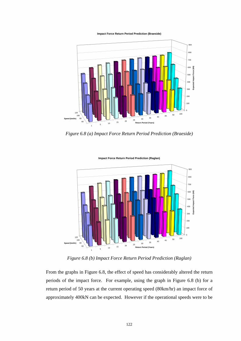
122
60
80100
120
1 5 10 15 20 25 30 35 40 45 50 100
0
100
200
300
400
500
600
700
800
900
Expe
cted
Impa
ct F
orce
(kN
)
Speed (km/hr)
Return Period (Years)
Impact Force Return Period Prediction (Braeside)
Figure 6.8 (a) Impact Force Return Period Prediction (Braeside)
60
80100
120
1 5 10 15 20 25 30 35 40 45 50 100
0
100
200
300
400
500
600
700
800
900
Expe
cted
Impa
ct F
orce
(kN
)
Speed (km/hr)
Return Period (Years)
Impact Force Return Period Prediction (Raglan)
Figure 6.8 (b) Impact Force Return Period Prediction (Raglan)
From the graphs in Figure 6.8, the effect of speed has considerably altered the return
periods of the impact force. For example, using the graph in Figure 6.8 (b) for a
return period of 50 years at the current operating speed (80km/hr) an impact force of
approximately 400kN can be expected. However if the operational speeds were to be

123
lifted to 100km/hr than the expected impact force for a 50 year return period would
increase to 560kN.
This has major implications for railways as operational speeds are likely to increase
in the future. Therefore if railway components are to have a long design life,
considerations for increased magnitudes of impact forces due to increased
operational speeds must be considered.
A correlation between the impact force magnitude, speed and wheel flat size for
empty and full wagons can be made from the data collected by the WCM and the
DTRACK simulations. The graphs in Figure 6.9 show the relationship between the
three parameters for the empty and full wagon scenario.
525
5075
100
20
40
60
80
100
120
0
200
400
600
800
1000
1200
Impact Force (kN)
Wheel Flat Size (mm)
Speed (km/hr)
Impact Force Prediction Based on Speed and Wheel Flat SizeEmpty Wagons
Figure 6.9 (a) Impact Force VS Speed VS Wheel Flat Size (Empty)

124
5 25 50 75 100
20
40
60
80
100
120
0
200
400
600
800
1000
1200
Impact Force (kN)
Wheel Flat Size (mm)
Speed (km/hr)
Impact Force Precition Based on Speed and Wheel Flat SizeFull Wagons
Figure 6.9 (b) Impact Force VS Speed VS Wheel Flat Size (Full)
As many railway operators’ wheel maintenance standards in Australia specify a
maximum allowable wheel flat size rather than a maximum allowable impact force,
the graphs in Figure 6.9 can be used to correlate an impact force against the speed of
the vehicle and wheel flat size. For example, the graph in Figure 6.9 can be used in
conjunction with the graph in Figure 6.7 so the maximum impact force can be
correlated back to a wheel flat size which can be used to compare against the current
wheel maintenance standards at Braeside and Raglan.
In the development of limit state design, the ‘worst case scenario’ is of greatest
interest to the designer. Therefore the full wagon scenario in Figure 6.9 (b) would be
used in the development of limit state methodology rather than the empty wagon
scenario where the impact forces are significantly lower.

125
6.6 Summary
The wheel impact force distribution graphs presented in Chapter 6 will be used in
Chapter 7 to establish the return periods and risk analysis for the development of
limit state design for railway track. The impact force distribution graphs presented
were based on data for a unique scenario that is not necessarily representative of all
railway traffic operating. However the methodology presented is expected to be
applied to other operating conditions.
For the development of a limit state design methodology for railway track,
allowances could be needed for the effects of varying parameters such as changes to
operating speeds, vehicle unsprung mass, vehicle suspension characteristics and the
wheel maintenance practices, as these parameters can greatly affect the magnitudes
of impact forces experienced in railway track. In Chapter 6 changes to these
operating parameters were investigated using the DTRACK model.
The DTRACK simulations found that impact forces were affected to any significant
extent only by changes to the parameters of speed and maintenance practices. The
effect of unsprung mass and suspension characteristics were negligible.
The wheel impact force distributions graphs in Figure 6.7 and 6.8 have shown that
increasing operational speed (if the maintenance standards were to remain the same)
would change the magnitude of impact force and return period predictions.
Therefore if the operational speeds were to be increased, the maintenance standards
would have to become more stringent to compensate, because changes to the
maintenance standards also had a significant effect on the magnitudes of impact
forces as seen in the graphs in Figure 6.9.

126
In addition to the consequences for design loadings, changes to operational
conditions would also have an impact on the business functions of a railway.
Consequences to the business operations may include items such as track access
charges, wheel maintenance standards and cost of track construction and
maintenance. The consequences to business due to the operational changes would be
further explained in the following chapter.

127
CHAPTER 7
Implications for Limit State Design of Railway Track
7.1 Introduction
The current railway standards in Australia such as the Prestressed Concrete Sleeper
Code (AS1085.14, 2003) are still based on outdated allowable stress principles as
mentioned previously in Chapter 2. Allowable stress principles have a number of
limitations such as ignoring ultimate element strengths, probability of failure and of
loads occurring and the risks associated with the structure.
Such limitations could lead to the over design of structures and hence uneconomical
design of the structures. Because of these limitations structural designs based on
allowable stress principles have become increasingly inadequate and the need has
arisen to design structures based on probability and material strengths (Allen, 1982).
This chapter will provide a background on limit state design and examine how the
wheel impact force distribution graphs shown in Chapter 6 can be used to establish a
limit state design methodology for railway track. As the Rail CRC project 5/23 was
primarily focused on the ‘Dynamic Analysis of Track and the Assessment of its
Capacity with Particular Reference to Concrete Sleepers’, this chapter will focus
primarily on a limit state design for a railway concrete sleeper.

128
7.2 Background on Limit State Design
7.2.1 Limit State Concepts
Allowable stress design examines the capacity of a structure by calculating the
elastic stresses in it due to the maximum expected loads, and comparing them with
allowable stresses. The allowable stress is equal to the failure stress of the material
divided by a safety factor. Safety factors for new materials were estimated in
comparison with those for traditional materials by taking into account the nature of
failure for the new material and its uncertainty or variability (Allen, 1982).
Allowable stress design provides the following inequality for design.
FSFf kk <
Where fk = Stress due to applied loads
Fk = Limit stress
FS = Factor of safety which depends on characteristic of failure of the
material
Allowable stress design has a number of limitations such as ignoring ultimate
material strengths, probability of failure and probability of loads occurring and the
risks associated with the structure. These limitations may lead to the design of
structures with larger or stronger elements and hence an uneconomical design of
structures. Because of these limitations, allowable stress design methodology
became increasingly inadequate and the need to design structures based on
probability and material strengths is needed (Allen, 1982).
Limit state theory introduces the concepts of partial safety factors, characteristic
loads and characteristic strengths based on a probability approach. It provides the
framework which will enable design to be more accurate and therefore more
economical. Limit state theory also enables research results to be incorporated into

129
standards as they become available, and guides further research by focusing attention
on deficiencies in knowledge (Hughes, 1980).
7.2.2 Limit State Methodology
The basis of the limit state approach is the application of statistics to establish the
probabilities of extreme load events occurring and then developing load factors as
margins of safety. Therefore, limit state design allows for a more logical design
process than implicit allowable stress design. The adoption of limit states also
permits the designer to vary the load factors for design and thus improving overall
economy of the design (Campbell and Allen, 1977).
The development of limit state approach has essentially five components
(Ellingwood and Galambos, 1982):
a. Develop statistical data to describe the basic load and resistance variables.
b. Establish procedures for calculating reliabilities of structural members and
systems. Ideally, the performance criteria should be based on a system
reliability requirement. However, current practice usually checks
performance on the basis of individual member behaviour.
c. Establish target reliabilities for design by analysing reliabilities associated
with structural members designed according to existing criteria. This
enables the probability based criteria to be related to existing acceptable
practice and provides the continuity that is necessary from one design
specification to the next.
d. Select a deterministic format that balances theoretical appeal with the need
for simple safety and serviceability checking procedures in professional
practice. Determine general load criteria suitable for all construction
materials.
e. Develop resistance criteria that are consistent with the load criteria selected
in step 4 such that reliabilities are close to the target values selected in step
3.

130
The calculation of limit state factors requires the probability distribution of each load
and resistance variable. The probability distribution must also characterise the
uncertainty in the variables that would be expected in structures in service. The limit
state factors must also allow for errors that may be in the data collection process such
as limited measurements, errors in modelling and variability in data etc.
In order to simplify and unify the present prestressed concrete sleeper code
(AS1085.14, 2003) it is suggested that the following principle be adopted. The
resistances, resistance factors and structural theory depend only on the material and
type of structure and will therefore be contained in material design aspects (for
example, expand the current concrete code AS3600 (2001) to accommodate railway
sleepers). The loads, load factors and main serviceability requirements depend only
on the use of the structure and will therefore be given in a new railway loading code
(for example, make AS1085.14 into a railway loading code).
All structures have two basic requirements in common: safety from collapse and
satisfactory performance of the structure for its intended use (Allen, 1982). Limit
states define the conditions in which a structure fails to satisfy these basic
requirements. A limit state condition is a condition where a structure or structural
element in some way becomes unfit for its intended purpose (Ellingwood et al.,
1982).
Limit state conditions are generally classified into three major categories:
(a) Ultimate Limit State, transformation of the structure into a mechanism that is
no longer capable of supporting the applied load without collapse or
excessive deformation.
(b) Serviceability Limit State, deformations, which affect the efficient use or
appearance of structural or non structural elements.
(c) Other considerations or limit states: fatigue, durability, fire resistance,
lightning etc.

131
For each limit state condition, the loads are multiplied by a load factor which takes
into account the probability of deviations of the load. When combinations of loads
are considered, the load factor may be decreased to take into account the reduced
probability of different loads acting simultaneously. The load factor may also be
adjusted by an importance factor to increase or decrease the safety of the structure
depending on the severity of the consequences. The limit state inequality can be
expressed as:
uRS φ≤*
Where S* = design action effect due to the factored design loads.
φRu= factored design capacity of a member
In the design of limit states the structural resistance, R and load effects, S are
represented in a reliability model and the relationship between the two parameters
are illustrated in Figure 7.1.
Figure 7.1 Probability density functions of load and strengths (Campbell and Allen,
1977)
From the graph, there is clearly a degree of safety if the load applied does not exceed
the component’s maximum sustainable load. The degree of safety is defined as the
safety factor, n and is usually expressed as;

132
n = Maximum Load/Actual Load
And if n = 1 than the component is on the point of failure
n < 1 then the component is in a failed state
n > 1 then the component is safe
Figure 7.2 provides the variations of safety factor with respect to load effects and
structural resistance. Generally the larger the safety factor, the less economical the
structure will be as the structure may be designed for loads that may never be
encountered in its service life.
Figure 7.2 Variations in probability functions with varying safety factors (Wright,
2000)
The benefits of variations in probability functions are that if the consequences of
failure are unacceptable or expensive, the designer is entitled to increase the safety
factor or increasing the strength of the component. Alternatively, if the consequence
of failure more acceptable and the expense is minimal, the designer may reduce the
safety factor to enable a more economic design as in temporary structures. Another
benefit of the reliability model is that it allows for combination of loads to be treated
as a single load effect and analysed using the same methodology.
The advantage of a limit state approach is that it allows the designer to define the
limiting state for individual or combination loads based on characteristic probability

133
distributions and applications of those loads. The designer also has the option select
the material strengths and other properties based on the degree of reliability that the
design requires.
The advantages of limit state concepts can be adapted to railway track engineering
such as developing a concrete sleeper based on the probability of forces that the
sleeper may encounter during service life. Limit state concepts also presents possible
cost savings through the ability to run higher speeds and axle loads on existing
infrastructure without wholesale changes. The adaptation of limit state concepts to
railway track engineering has the potential to develop a more economic railway
based on probabilistic loads.
7.2.3 Material Resistance
At present, Australian Standards have the Concrete Structures Code (AS3600, 2001)
for reinforced and prestressed concrete structures. The principal objective of the
code is to provide designers with nationally acceptable unified rules for the design
and detailing of concrete structures and elements, with or without steel reinforcement
or prestressing tendons, based on the principles of structural engineering mechanics.
The secondary objective is to provide performance criteria against which the finished
structure can be assessed for compliance with the relevant design requirements
(AS3600, 2001).
AS3600 (2001) is a fairly comprehensive code that covers the reliability of concrete
structures under different loading conditions and environments. The principles for
the design of concrete sleepers are similar to any structural concrete design.
However the current AS3600 (2001) does not cover high frequency and sudden
dynamic impact loads that are experienced by prestressed concrete sleepers.
Experimentation by Pandrol Australia (1987) examining the effect of rail pads to the
dynamic loads induced into prestressed concrete sleepers in Queensland Railways
found that the failure of some concrete sleepers has been caused by excessive
flexural vibration. The Pandrol report also found that the properties (such as elastic
134
modulus and stiffness) of the rail pad also influence the dynamic responses of the
sleeper. Therefore it is important to understand the effects the properties of the rail
pad has on concrete sleeper loadings.
The responses of prestressed concrete sleepers are currently being researched under
the Rail CRC Project 5/23 at the University of Wollongong. The main aim of the
research at the University of Wollongong is to develop a better understanding of the
dynamic responses of concrete sleepers. The project will also investigate the
different responses concrete sleepers have to different rail pad properties. The
proposed research will be working in conjunction with the University of Wollongong
to develop limit state factors for recommendation to Standards Australia.
Before limit state factors can be developed for prestressed concrete sleepers, two key
issues must be understood. The first is the understanding of the responses concrete
sleepers have to high frequency loadings that are caused by railway traffic. The
second is establishing the probability of significant forces due irregularities at the
wheel/rail contact face (described in the following chapters).
7.2.4 Load Effects
Most structural loads may be thought of as consisting of a basic load parameter
which is essentially independent of the structure; a modelling parameter that
transforms the spatially and temporally varying load into an equivalent uniform (and
usually static) load for analysis and design purposes, and finally, an influence
coefficient or analysis factor that transforms the uniform load into a structural action
such as a beam moment (Ellingwood et al., 1982).
The loading parameter for railway track is extremely complicated compared to
structural loads, due to the dynamic behaviour of the loads and the impact loading
due to defects at the wheel/rail interface. Studies undertaken in Japan by Wakui and
Okuda (1999) have classified the effects of railway loading into two categories to
simplify load effects induced into railway track;
Quasi-static wheel loading – forces generated by vibrations of the vehicles
unsprung mass

135
Impact wheel loading – forces generated by collisions between the vehicles
unsprung mass and the railway track.
By categorising the loading effects, limit state factors can be derived for each
condition and the effects analysed separately. The study undertaken by Wakui and
Okuda (1999) was mainly concerned with the loading effects at the rail seat. The
forces were measured at the rail seat because designers can design the concrete
sleeper and the subgrade to transmit these forces.
However, the study does not develop a methodology for limit state factor
development or provide any statistical data for wheel flat defects experienced in
Japan and only presents the effects of various wheel flats at various speeds on rail
seat loadings.
The adoption of limit state principles into standards is not a new concept as most
structural codes in Australia and internationally has incorporated these principles.
However, this literature review has found that railway design standards in Australia
and internationally are not based on limit state principles.
Wakui and Okuda (1999) have identified that the primary hindrance to developing
the standards from conventional allowable stress principles to contemporary limit
state principles has been the understanding of the complex dynamic characteristic of
railway track. The defects at the wheel/rail interface have been identified as the main
cause by many researchers such as Tunna (1988), Jenkins et al. (1974) and Frederick
(1978) that generate the largest dynamic forces and will be examined in the
following chapter.

136
7.3 Definition of a ‘Failed’ Concrete Sleeper and Limit State
Conditions
In the development of a limit state design methodology for concrete sleepers, a clear
definition of concrete sleeper failure must first be established as the design limit state
conditions are heavily dependent on the definition of failure; i.e. what limiting
conditions can be defined that relate to the operations of a railway system.
In structural engineering, the definition of failure is when the structural element is
unable to sustain the bending or shear or axial actions imposed onto the structure.
However, this definition of failure cannot be applied to railways as the functions of a
concrete sleeper are different from the functions of a structural element in a building.
In Australia, railway organisation will condemn a sleeper when its ability to hold top
of line or gauge is lost. These two failure conditions are caused by the following
conditions:-
a) Abrasion at the bottom of the sleeper causing loss of top;
b) Abrasion at the rail seat causing a loss of top;
c) Severe cracks at the rail seat causing the ‘anchor’ of the fastening system
to move and spread the gauge;
d) Severe cracks at the midspan of the sleeper causing the sleeper to ‘flex’
and spread the gauge; and
e) Severe degradation of the concrete sleeper due to alkali aggregate
reaction.
It should be noted that abrasion and alkali aggregate reaction are due to the failure of
the concrete material and not structural failure of the sleeper as a structural element.
However, material factors such as abrasion and chemical resistance could be
included in a revised version of the Prestressed Concrete Code (AS1084.14, 2003) in
a manner similar to that adopted by the Concrete Structures Code (AS3600, 2001).

137
The definition of the structural failure of a concrete sleeper should therefore be based
on the concrete sleepers’ inability to hold top of line and gauge caused by the loading
environment in which the sleeper is exposed to.
It should also be noted that unlike the traditional structural engineering situation
where the failure of a single element can lead to catastrophic collapse of a major part
of a structure, the failure of a single sleeper does not constitute a failed track
structure or failure of the systems ability to carry railway traffic at full capacity.
Therefore, the number and arrangement of failed sleepers in a given cluster must be
given consideration as certain clusters of failed sleepers would constitute a failed
track structure.
The number and arrangement of sleeper cluster failure should be determined by the
track asset owners as each organisation in Australia has their own separate sleeper
cluster standards. The determination of the probability of sleeper clusters failing can
be calculated through a series of Monte-Carlo simulations and the level of risk
associated with cluster failure can also be established. However, these simulations
and risk assessments will not be presented in this thesis as it falls outside the scope of
the project.
The concept of limit states design defines a condition when the element or system
ceases to fulfil its design constraints and is no longer fit-for-purpose. Such a
situation is deemed to be ‘failure’ of the element or system. The outcome of this
failure can be replacement or repair of the element or system, depending upon which
design constraint has been exceeded, i.e. depending upon the type of failure
condition. For example, if a concrete beam in a building exceeds the ultimate design
limit state, replacement is usually the only option. However if the beam has only
exceeded the serviceability limit state (such as excessive cracking) than repair may
be all that is required.
For railway concrete sleepers, the design limit state conditions would have to be
slightly different to the traditional structural approach and should take into
consideration the railway track’s ability to continue to operating. Proposed below

138
are three limit state conditions that are believed to encompass the design limit states
relevant to the design of railway concrete sleepers.
1. Ultimate Limit State
A single once off event (for example a severe wheel flat or dipped joint) that
generates enough force to fail a single concrete sleeper due to that one event. Failure
under such a severe event is expected to fit within failure definitions (c) and (d)
above.
2. Damageability Limit State
A single concrete sleeper that has accumulated damage progressively over a period
of years to a point where it is considered to have reached failure. Such failure could
come about from excessive accumulated abrasion or from cracking having grown
progressively more severe under repeated loading impact forces over its lifetime.
Failure due to accumulated damage fits within failure definitions (a) to (e).
3. Serviceability Limit State
This limit state defines a condition where sleeper failure is beginning to impose some
restrictions on the operational capacity of the track. The failure of a single sleeper is
rarely if ever a cause of a speed restriction or a line closure. However, when there is
a failure of a cluster of sleepers, an operational restriction is usually applied until the
problem is rectified.
The proposed limit state conditions above follow a similar format to that in the
current structural standards in the Standards Australia series. The limiting conditions
proposed would form the basis for designing a concrete sleeper based on both
engineering and commercial risks and hence a more realistic design outcome for
railway track can be achieved.

139
7.4 Formulation for the Calculation of Design Wheel Load
The proposed methodology for the calculation of the design wheel load is similar to
the methodology that is found in the current structural standards (such as Loading
Code AS1170, 2002) found in Standards Australia, where the design load (P*) is
determined by a series of load combinations and load factors that are based on the
probability and return periods of loads occurring. In structural engineering (AS1170
Clause 4.2.1, 2002), one of the design actions (P*) is determined by:-
P* = 1.2G + 1.5Q Equation 7.1
Where, G = Permanent Load Q = Live Load
Equation 7.1 can be modified to suit the design of railway loadings where the design
action load (P*) can be transformed into a design wheel/rail force (F*). Then
Equation 7.1 would become:-
F* = 1.2 Fs + Fi Equation 7.2
Where, Fs = Static wheel load Fi = Wheel/rail impact force
The calculation of the static wheel load (Fs) would be based on the maximum
allowable load limit set by the rail track owner. For the case of Braeside and Raglan,
the maximum allowable load limit was 28.5tonnes/axle which would be used in those
cases for the static wheel load value (Fs). The 1.2 factor for the static axle load is to
allow for the overloading of the vehicles and is based on the Braeside and Raglan
graphs in Figure 5.14 where a number of vehicles were loaded up to 20% above the
target axle load.
The calculation for the wheel/rail impact force (Fi) would be determined by either the
defects at the wheel or rail interface and not both as the resultant impact force of
these two events are independent of one another. For example, a wheel flat

140
impacting on a dipped joint is assumed to result in the same magnitude of impact
force from a normal round wheel impacting on a dipped joint.
Therefore, there needs to be two methods for determining the design wheel/rail force
(Fi) where it can either be:-
Fi,w = Design impact force caused by wheel defects; or
Fi,r = Design impact force caused by rail defects.
The two design wheel rail forces above will form the basis for developing the design
wheel/rail force for railway track. The calculation of the design wheel force caused
by the wheel (Fi,w) or rail (Fi,r) would be determined by a series of factors that are be
based on the probability of occurrence of wheel or rail interface defects within the
lifetime of the sleeper.
The wheel/rail impact force caused by rail defects (Fi,r), such as dipped joints, will
not be investigated in this thesis due to time constraints and because the data required
would fall outside the scope of the research project.
The use of factors in the calculation of design forces is not a new concept. The
current Australian Standards structural series such as the Loading Code (AS1170,
2002) already contain loading factors within the standards which are based on the
probability and return periods of extreme events occurring. For example, the
calculation of design wind gust speed (AS1170.2 Clause 3.2.2, 2002) is calculated
by:-
dtscatzRsit MMMMVV ),(, =β Equation 7.3 Where, Vsit,β = Design site wind speed VR = Gust wind speed M(z,cat)= Terrain category factor Ms = Wind shield factor Mt = Topographic factor Md = Wind direction factor

141
The factors (M(z,cat), Ms, Mt, Md) used for the calculation of the design wind speed are
determined by the parameters (such as structure location and direction) that may
increase or decrease the design wind speed of the structure. The derivation of these
factors is based on comprehensive wind speed data from which probabilities and
return periods can be determined.
When the designer has determined the design wind speed presented in Equation 7.3,
the designer would then be able to calculate the actions on the structural elements via
a computer assisted design program and design the structure accordingly.
The calculation of the design wheel/rail force can be analogous to the calculation of
the design wind speed for structural engineering where design wheel/rail force can be
determined by a series of factors based on probability and return periods drawn from
a comprehensive set of data. Similar to structural engineering, once the design
wheel/rail force has been determined, the designer may then utilise a computer
assisted design program such as DTRACK to calculate the actions on the railway
track components and design those elements accordingly.

142
Methodology for the Determination of the Design Wheel/Rail Force Due to Wheel Defects (Ft,w)
The proposed calculation of the design wheel/rail force due to wheel defects (Fw*) is
proposed to be calculated by the following equation:-
wiswt FFF ,),( 2.1 += Equation 7.4
The determination of the static wheel force (Fs) was mentioned earlier and is based
on the maximum allowable axle load specified by the railway track owner. The
impact force caused by wheel defects (Fi,w) is calculated by the following equation:-
IFFIwmimpwi kkkFF =, Equation 7.5
Where, Fimp = Impact force caused by a wheel defect kwm = Wheel maintenance factor kI = Track importance factor kIFF = Impact force factor
The calculation of the impact force caused by a wheel defect (Fimp) could be based on
the maximum allowable wheel impact force specified by the railway track owner and
would be the ‘base case’ for the design of railway track forces. For example, the
code of practice for the defined interstate network in Australia (ARA, 2003), the
maximum allowable P2 force allowed to be induced into the track is 230kN for
freight vehicles, therefore for this case, the impact force (Fimp) would be 230kN.
The determination of the factors (kwm, kI and kIFF) introduced in Equation 7.5 are
analogous to the calculation of the design wind speed in Equation 7.3 where the
factors are based on return periods and probabilities of occurrences.

143
Wheel Maintenance Factor (kwm)
The proposed wheel maintenance factor (kwm) is based on the frequency of wheel
maintenance and the level of wheel maintenance standards used by the railway
operator. The wheel maintenance factor allows for the variability in wheel
maintenance intervention strategies and maintenance standards adopted by different
operators. For example, in a scenario such as the interstate railway network where
there are numerous rail operators with various wheel maintenance standards and
strategies, the wheel maintenance factor (kwm) can cater for those various standards
and strategies to minimise the probability of failure for the railway track.
Table 7.1 shows three wheel maintenance factors that are proposed which would be
based on the frequency of intervention, intervention strategy and standards applied to
the maintenance of rollingstock wheels.
Table 7.1 Proposed Wheel Maintenance Factors
Wheel Maintenance
Group
Wheel Maintenance Characteristics Wheel Maintenance Factor (kwm)
Group 1 A very high standard of wheel maintenance in which wheel tread defects are detected and removed quickly. The maximum wheel tread defects tend to be small.
0.9
Group 2 This group includes railway lines that operate an impact detector to assist the operator to identify and rectify the wheel defects. The wheel maintenance standard in this group does not represent the highest achievable wheel maintenance standard; rather, the early detection of wheel defects reduces the risks of further damage to the railway track. The mineral wagons traversing Braeside and Raglan would fit into this category.
1
Group 3 This group would include situations where vehicles are subjected only to visual inspection and detection by drivers.
> 1
The wheel impact maintenance factors (kwm) in Table 7.1 would help determine level
of risk a railway track owner is willing to accept from the railway operator. The
determination of the wheel maintenance factor should be based on risk assessments
carried out by the railway track owner and operator.

144
Track Importance Factor (kI)
The proposed track importance factor (kI) is based on the level of acceptable
commercial risk (such as delays to operations) the railway track owner is willing to
accept. For example, in a scenario where failed sleepers affect the operation of a
profitable heavy haul railway carrying high traffic volumes, the consequences would
normally be much greater and of more concern to the track owner and train operators
than the same failure of sleepers on a branch line with low traffic volumes.
Therefore, sleepers installed on a heavy haul line should be designed with a lower
risk of failure than sleepers on a branch line.
The track importance factor (kI) should not attempt to cover extreme events such as
derailments as these events arise from exceptional circumstances and it would be
impractical and uneconomical to design sleepers based on such events. Therefore,
the ‘cost’ for the loss of human life for example should not be considered in
determining the track importance factor (kI).
Commercial risks associated with changes to operational conditions such as
operational speeds are not part of the track importance factor (kI). These matters
would be taken into account by the impact force factor (kIFF) presented in the
following sections.
Table 7.2 presents possible values for the track importance factor (kI) and the
categories of railway track associated with the factor. The factors are ranked
according to importance, where 1 is the greatest importance and 4 is the least
importance.
The track importance categories proposed are a reflection of the typical range of
railway track that is found in Australia. The track importance factors should also be
able to be applies to other railway operations such as passenger, cane tram operations
or light rail.

145
Table 7.2 Possible Track Importance Factor Values
Track Importance
Category
Line Characteristics Possible Track
Importance Factor (kI)
Category 1 Lines which meet the one or more of the following criteria:- a) The sole or critically important source of revenue
to the business; b) Consumes a major portion of the organisations
maintenance budget; c) Relatively short delays to services can have a
significant impact on reputation, profitability and/or service obligations;
d) Traffic is overwhelmingly of a single type of key importance to the business; and
e) Restricted track maintenance windows. Examples would be heavy haul or inner city suburban lines.
1
Category 2 Lines which meet some of the following criteria:- a) Carry mixed traffic producing a significant
income to business; b) Consume a large part of the maintenance budget; c) Short delays can be tolerated with limited effect
on reputation, profitability and/or service obligations; and
d) Regular track maintenance windows available. Examples would be lines such as freight connections between major city centres.
0.95
Category 3 Lines which meet most of the following criteria:- a) Carry routine mixed traffic contributing to
business revenue; b) Receives regular programmed routine
maintenance; c) Low to average volumes of traffic compared to
the business’s prime operations; and d) Long delays can influence reputation,
profitability and/or service obligations. Examples would be lines that carry freight connections between city centres, but are not as important as Category 2.
0.90
Category 4 Lines which meet all of the following criteria:- a) Marginal profitability; b) Infrequent or minor maintenance requirements; c) Delays to services are rarely of serious
consequence; and d) Irregular, infrequent traffic. Examples would be branch lines.
0.85

146
Impact Force Factor (kIFF)
The impact force factor (kIFF) is based on the return periods and consequences of
changing operational characteristics, in particular changing operational speeds. The
formulation of the impact force factor would be analogous to the return factors found
in the Australian Rainfall and Runoff (2005) publication, where calculation of the
quantity of rainfall is dependent on and determined by the return periods and design
life of the structure. In the case of railway loading calculations the impact force
magnitude would also be dependent on and determined by the return periods and
design life of the railway track.
To illustrate how the return periods and probability of occurrence can be applied, the
data from the Braeside and Raglan wheel impact detectors will be used to calculate
the wheel impact factors for railway loadings. It should be noted again that the data
for Braeside and Raglan is for a single unique railway operation; for a more
comprehensive set of factors, more data of various wheel impacts from around
Australia would be needed.
The graphs in Figure 7.3 (a) and (b) shows the impact factors for the Braeside and
Raglan sites respectively. The dotted lines within the graph represent the impact
force factor for a given return period and speed as indicated by the values on the left
hand side of the graph. The dots were calculated by ‘normalising’ the impact forces
against the impact force generated at 60km/hr, 1 year return period (see graphs in
Figure 6.8). For example:
The base case impact force at Braeside for a speed of 60km/hr, 1 year return period
was 230kN, so the impact force factor for the base case was:
Impact force factor for 60km/hr, 1 year return period = 230/230
= 1

147
For 80km/hr, 50 year return period at Braeside, the impact force was 400kN,
therefore the impact force factor was calculated by:-
Impact force factor for 80km/hr, 50 year return period = 400/230
= 1.74
Near the left side of the graph in Figure 7.3 (a) and (b) are the speeds for the
respective impact force factors for each of the dotted lines. The lines of best fit
within each graph were drawn in by the writer and are representative of the dots for
the 60km/hr and 120km/hr speeds. The line of best fit for the 90km/hr speed was an
interpolation between the two other lines of best fits.
Impact forces generated by wheel defects under 60km/hr were not considered in the
graphs in Figure 7.3 as the forces are too small to have any significant effect on the
design of track components in the current common situations.
Impact Force Factor (Braeside)
0.00
0.50
1.00
1.50
2.00
2.50
3.00
3.50
0 10 20 30 40 50 60 70 80 90 100 110
Return Period (Years)
Impa
ct F
orce
Fac
tor
120km/hr
90km/hr
60km/hr
60km/hr
80km/hr
100km/hr
120km/hr
Lines of Best Fit
Lines of Best Fit
Lines of Best Fit
Figure 7.3 (a) Impact Force Factor for Braeside

148
Impact Force Factor (Raglan)
0.00
0.50
1.00
1.50
2.00
2.50
3.00
3.50
0 10 20 30 40 50 60 70 80 90 100 110
Return Period (Years)
Impa
ct F
orce
Fac
tor
120km/hr
90km/hr
60km/hr
120km/hr
100km/hr
80km/hr
60km/hr
Lines of Best Fit
Lines of Best Fit
Lines of Best Fit
Figure 7.3 (b) Impact Force Factor for Raglan
From the lines of best fit within each of the graphs in Figure 7.1 (a) and (b), an
equation of the lines can be derived based on the return periods and operational
speeds for both the sites.
The impact force factor (kIFF) calculated from Figure 7.1 (a) and (b) would be:-
Braeside: 73.0029.000278.0 −+= vRkIFF Equation 7.6 (a)
Raglan: 56.0029.000178.0 −+= vRkIFF Equation 7.6 (b)
Where, R= Return period (years) v= Velocity
149
7.5 Case Study
Assuming that the current operating speed at Braeside was to be increased to
100km/hr from 80km/hr, would the current concrete sleepers be able to carry the new
loadings under the ultimate condition of 50 years?
The calculation of the wheel/rail force from wheel defects using Equation 7.4
requires determination of Fs and Fi,w. For the current traffic operating at Braeside,
the maximum allowable axle load (Fs) is 28.5tonnes. Therefore,
Fs= 28.5 x 9.81
= 280kN/axle
= 130kN/wheel
From Equation 7.5 the design wheel/rail impact force (Fi,w) caused by wheel defects
is:-
IFFIwmimpwi kkkFF =,
As mentioned previously the base case impact force (Fimp) can be based on the
railway track owners specified maximum allowable impact force. For this example,
the base case impact force was suggested in Section 7.3 to be 230kN.
The wheel maintenance factor (kwm) for this case study would be Group 2 in Table
7.1 whereas the track importance factor (ki) would be Category 1 in Table 7.2,
giving:
kwm= 1
ki = 1
The impact force factor (kIFF) would be determined from Equation 7.7 as follows:-
For the 80km/hr case For the 100km/hr case 39.080019.05000185.0 −×+×=IFFk 39.0100019.05000185.0 −×+×=IFFk
73.1=IFFk 31.2=IFFk

150
The design wheel/rail force (Ft,w) for both cases becomes: For the 80km/hr case For the 100km/hr case
wiswt FFF ,),( 2.1 += wiswt FFF ,),( 2.1 +=
IFFIwmimpswt kkkFFF += 2.1),( IFFIwmimpswt kkkFFF += 2.1),( 73.1112301302.1),( ×××+×=wtF 31.2112301302.1),( ×××+×=wtF
wheelkNF wt /554),( = wheelkNF wt /687),( =
Therefore, if the current operating conditions were to change from 80km/hr to
100km/hr, it would be expected that there would be approximately 20% increase in
wheel impact force over a 50 year design life.
Checking these calculations with the graph in Figure 6.8 (a) where for a 50 year
return period, the expected wheel impact force for operating speeds of 80km/hr and
100km/hr are 400kN and 565kN respectively;
For the 80km/hr case For the 100km/hr case kNFF swt 4002.1),( += kNFF swt 5652.1),( += 4001302.1),( +×=wtF 5651302.1),( +×=wtF
wheelkNF wt /568),( = wheelkNF wt /733),( =
The difference in wheel impact force between the design wheel load and the Braeside
data in Figure 6.8 (a) for the 80km/hr and 100km/hr case was 4% and 2%
respectively. Therefore the methodology developed in Section 7.3 only has a small
margin of error and is adequate for design.
From the impact force versus speed versus wheel flat size graph in Figure 6.9 (b), a
wheel flat size can be correlated to the calculated impact forces for the 80km/hr and
100km/hr case. Table 7.3 shows the corresponding wheel flat to the calculated
design wheel/rail force (Fi,w) for a 50 year design life.
Table 7.3 Proposed Track Importance factors Vehicle Speed Design Wheel/Rail Force Corresponding Wheel Flat
80km/hr 534kN/wheel 60mm 100km/hr 687kN/wheel 61mm

151
The corresponding wheel flats in Table 7.3 can now be used to calculate the bending
moments in a concrete sleeper using the DTRACK computer model. Assuming that
the parameters of the existing track conditions at Braeside are the same as the
conditions used in Benchmark II (refer to Chapter 5) and is summarised below in
Table 7.4
Table 7.4 Braeside Track Parameters
Component Description Rail AS 60kg/m
Gauge 1065mm Rail Pad HDPE
Sleeper Type M270 Pandrol Concrete Sleeper (refer to Drawing No201-05 in Appendix XX)
Sleeper Spacing 685mm Track Bed Type Medium Stiffness (Stiffness 50.1MN/m, Damping
159kNs/m)
The properties of a typical heavy haul wagon operating at Braeside are shown in
Table 7.5 below.
Table 7.5 Braeside Parameters Component Description
Gross Vehicle Mass 106 tonnes Axle Spacing 1780mm
Sideframe Mass 500kg Sideframe Mass Moment
of Inertia 500kg.m
Suspension Stiffness 2MN/m Suspension Damping 0kNs/m
Wheelset Mass 1400kg Wheel Radius 457.5mm
Wheel Profile Radius at Contact
360mm
The parameters in Table 7.3, 7.4 and 7.5 were entered into DTRACK to calculate the
bending moments of the rail seat (M*railseat) for the two speeds 80km/hr and
100km/hr. Table 7.6 shows the resulting bending moments.
Table 7.6 Rail Seat Bending Moment M* Vehicle Speed Design Wheel/Rail Force Rail Seat Bending Moment (M*)
80km/hr 554kN/wheel 38.1 kN.m 100km/hr 687kN/wheel 39.4 kN.m

152
From the Drawing No 201-05 found in Appendix XX, the ultimate bending moment
capacity (Mu) of the concrete sleeper that is found at the Braeside site is as follows
(calculation of the sleeper design capacity can be found in Appendix XX):-
Mu = 54.9kN.m
φMu = 0.85 x 54.9kN.m (φ value from AS3600 Clause 2.4.2, 2001)
= 47kN.m
*MM u >∴φ from Table 7.6
The calculated design sleeper bending moment at the rail seat (φMu) and the design
rail seat bending moment (M*) have shown that there is still approximately 15%
reserve of strength in the current concrete sleepers at Braeside based on a 50 year
return period.
The case study presented in this section assumes the concrete sleeper experiences
complete flexural failure at φMu which is the ultimate limit state prescribed in
Section 7.2.
The material reduction factor (φ) could possibly be increased for concrete sleepers
because they are manufactured in an environment where properties such as strength,
fabrication tolerances and quality of materials are well controlled. The stringent
quality control used to manufacture concrete sleepers increases the reliability of the
sleepers.
7.6 Implications for Railway Businesses
Transforming the current Standard Australia Prestressed Concrete Sleeper Code
(AS1084.14, 2003) from allowable stress to limit states methodology would have
implications for railway businesses. Limit states methodology would open up a
range of possibilities for railway businesses such as a more accurate evaluation of
capacity of the track asset, asset and risk management and more realistic track access
charges.

153
The accurate evaluation of the track asset would allow track asset owners to develop
better maintenance strategies such as replacement of the asset. Therefore, the track
asset owner may be able to increase the speeds and payloads of the rollingstock
based on a limit state evaluation of the track structure, without having to replace
hundreds of thousands of sleepers.
Using limit state principles for design and evaluation also allows track owners to
better manage the railway track asset based on probability and risk. For example, the
track owner may be able to better manage and determine the level and quality of
track maintenance based on the level of acceptable risk.
Limit state assessment of railway track also allows asset managers to calculate the
whole life of costing for the track asset with greater accuracy as probabilities of track
failure can be established. Limit state methodology would also better allow asset
managers to assess the longevity of the railway track components which could have
significant potential cost savings for the track owner. Risk management for railway
track will also become more accurate as the definition of track failure and its
consequences become clearer.
Track access charges can also be influenced as a result of limit state evaluation for
railway track. As risk management becomes more reliable, railway operators and
track asset owners would be able to negotiate access charges based on the level of
acceptable risks for both parties. For example, a rail operator would be able to
negotiate track access charges based on the level of their wheel maintenance
standards as the risks and consequences of failure can be estimated in terms of costs.
The implications of a limit state design is beneficial for business as it gives railway
operators and track owners’ flexibility to manipulate the design and standards of
railways based on their assessment of acceptable risks. The effect would be an
improved view of railways as a more viable means of transport.

154
7.7 Summary
This chapter has presented a limit state design methodology for railway loadings
based on the wheel/rail data presented in Chapter 5 and 6. The limit state design
methodology developed in this section is based on a single unique track and train
scenario; for a more comprehensive methodology, more wheel/rail data covering all
the various operational conditions in Australia would be needed.
Definitions of failure for railway track were also presented in this chapter based on
Australian railway organisations’ definition of sleeper failure, where the sleepers
ability to hold top of line or gauge is lost. Three limit state conditions were therefore
proposed which follow a similar format to those in the current Standards Australia
series.
A methodology for the calculation of the ultimate design wheel load was presented,
proposing a series of factors based on the probability of occurrence and the return
periods of wheel impact forces. The factors took into consideration the commercial
risks associated with track failure, reflecting the typical range of railway track found
in Australia.
A case study was presented in this chapter, which provided an example of how the
limit state methodology developed could be used to assess the capacity of the
existing concrete sleepers at Braeside. The case study found that under the current
Australian Standard for Concrete Structures design, the existing concrete sleepers at
Braeside do possess reserves of strength.
The development of limit states also has implications for railway businesses as it
provides a realistic evaluation of track performance, asset and risk management
become more reliable, possibly influencing determination of determination of track
access charges for operators. Limit state principles may also allow engineers to
design a more efficient railway track, leading to improvement of the profitability and
viability of railways as an alternative form of transport.

155
CHAPTER 8
Conclusions
8.1 Introduction
This thesis has presented a limit state design methodology for railway track for
recommendation to the Standards Australia next review of the Prestressed Concrete
Sleeper Code (AS1085.14, 2003). In the development of a limit state design
methodology for railway concrete sleepers, a comprehensive set of wheel/rail force
data for a unique railway operation has been collected and analysed to calculate the
probabilities and return periods of occurrences. The collected data was used in
conjunction with DTRACK to produce a limit state design methodology that can be
adapted to other railway operations and scenarios. The structure of this thesis had
five main parts:-
1. A review of the current Standards Australia and individual railway
organisations standards for railway track design, maintenance and operations;
2. The completion and benchmarking of the DTRACK model which will be
eventually become commercially available for the Australian railway
industry;
3. Presented a comprehensive set of wheel/rail impact force measurements that
was collected by the Teknis Wheel Condition Monitoring system;
4. Established a probabilistic analysis of the wheel/rail force distributions and
investigated the consequences of varying parameters to the impact force
distributions; and

156
5. The development of limit state factors and design methodology based on the
data collected at Braeside and Raglan.
8.2 Findings and Conclusions
The traditional methodology and current Australian Standards (AS1085.14, 2003)
used to design railway track is based on allowable stress principles. The design of
railway track based on allowable stress principles have a number of limitations
which include:-
- Neglect of material ultimate strengths;
- Ignoring the probability of failure and loads applied to the structure; and
- Ignoring the risks associated with failure of structural elements.
The limitations of allowable stress principles may lead to over-design and hence
uneconomical design of the railway track. Therefore there is a need to evolve the
current Concrete Sleeper Code (AS1085.14, 2003) from allowable stress principles
to a more realistic design philosophy.
Limit state principles allows for the design of the structural elements based on the
probability of occurrences, definitions of structural failure and risks associated with
failure. It provides a framework which will enable designs to be more accurate and
hence more economical. Limit state principles also allows designers to define the
failure conditions based on probability load distributions and design the structural
element based on the material strengths and degree of reliability required. Therefore
evolving the current Australian Standards Prestress Concrete Sleeper Code
(AS1085.14, 2003) from allowable stress principles to limit state principles has both
practicality and commercial benefits by reducing risks and improving productivity
for railway organisations.
As part of the goal in developing a limit state methodology for railway track, a
dynamic model was needed to investigate the complex interaction between vehicle
and track. The dynamic model chosen had to meet the criteria set by the Rail CRC
157
and had to demonstrate potential for further development. For these reasons the
Dynamic TRACK (DTRACK) model was identified as the best model for further
development and research.
The DTRACK model presented in this thesis is the completed revised version of the
DTRACK model presented by Steffens (2005). The original author of the program
(Cai, 1992) was contracted to correct the problems with DTRACK that were
identified by Steffens (2005). In addition a programmer had also been contracted to
finish the user friendly interface for DTRACK initiated by Steffens (2005).
Although the general structure of the DTRACK model had not changed, many of the
original features have been upgraded and improved. Improvements such as library
maintenance, data management and graphing abilities were included into the
upgraded DTRACK. The development of the DTRACK model was completed
within this thesis and is ready to be distributed to the Australian railway industry and
research community.
To test the reliability of the DTRACK model, a benchmarking exercise (known as
Benchmark II) was established where the results of DTRACK were benchmarked
against six other dynamic track models. In addition, Benchmark II compared the
results of all the participating models against field data which was collected at Lara
on the Melbourne to Geelong standard gauge railway track in Australia.
The results of Benchmark II found that the majority of the requested output
parameters of DTRACK was in good agreement with the results of the other
benchmarked models and the field data. However, Benchmark II also identified a
few issues with the outputs of the DTRACK model, where the magnitude of shear
force in the rail was too low and the bending moment of the sleeper contained many
peaks and dips in the magnitude which was not seen in the results of the other
models and field data.
The original author of the DTRACK model (Dr Zhenqi Cai) has been notified of the
problems and was addressing them at the time of writhing this thesis. The
uncharacteristic results of the DTRACK model did not affect the peak magnitudes of

158
the bending moment results and hence would not impede on the final outcomes of
this research.
In the establishment of a limit state methodology for railway track, a comprehensive
set of wheel/rail force data was needed. This thesis only examined the impact forces
caused by wheel defects for two main reasons:-
3. Wheel defects occur at random and have a high probability of occurring;
and
4. Impact events caused by wheel defects are not localised (such as dipped
joints) and can impact at random along a given section of railway track.
The wheel impact force data was collected by the Teknis wheel conditioning
monitoring system at Braeside and Raglan in Queensland. The data collected from
the WCM at Braeside and Raglan represented a single unique scenario (a heavy haul
line) and is not representative of the variety of railway operations in Australia.
However, the purpose of this thesis is to establish a limit state methodology that can
be adapted to other railway operational scenarios, therefore the data collected will be
used to establish a limit state design methodology for railway track.
The data collected from the Braeside and Raglan site showed that the impact force
distributions were heavily dependent on parameters such as:-
- Wheel maintenance practices and strategies;
- Vehicle speeds; and
- Driver behaviour of the vehicles.
The distribution of the impact forces that were presented formed the basis of
establishing a limit state design methodology for railway track. However, the data
collected from Braeside and Raglan only represents the current operating conditions
and does not consider future changes in operations such as speeds and wheel
maintenance practices which can greatly change the impact force distributions.

159
To predict the probabilities of occurrence and return periods of impact forces due to
future operating conditions, the DTRACK models was used to simulate the effects of
varying parameters such as operational speed, unsprung masses, suspension
characteristics and maintenance practices. The DTRACK simulations found that
speed and maintenance practices greatly affected the impact force magnitude and
will be used to investigate the changes to the impact force distributions of Braeside
and Raglan. The impact force distributions were recreated to accommodate the
changes of impact force magnitudes due to varying parameters.
The consequences of varying parameters dramatically changed the impact force
distributions and hence probability of occurrence and return periods. This has major
implications for the establishment of limit state design for railway track as the likely
changes in operational characteristics will significantly affect the magnitude of
impact forces and their distributions.
The concept of limit state design is dependent on a set of limit state conditions which
is based on the definition of structural failure. In the case of railways, the proposed
definition of concrete sleeper ‘failure’ is based on the sleepers’ inability to hold top
of line and gauge caused by the loading environment to which it is exposed to.
However, the failure of a single sleeper does not constitute the failure of the track
structure and does not compromise the railway tracks ability to carry traffic.
Therefore the limit state conditions should also consider the failure of sleeper
clusters based on each railway track owners own standards. The limit state
conditions proposed in this thesis are based on the economic consequences of failure
and should not be based on extreme conditions such as a derailment scenario.
The limit state methodology proposed in this thesis is analogous to the Australian
Standards Loading Code (AS1170, 2003) where the design load of a structural
element is determined by load factors and combinations based on the probability of
occurrence and return periods. This thesis presented a methodology for the
determination of the load factors based on the maintenance, track importance, return
periods and risks associated with failure, which is comparable to the calculation of
the design wind speed in Standards Australia Wind Code (AS1170.2, 2002).

160
A case study using the developed limit state methodology for railway track was also
presented in this thesis. The case study compared the capacity of the current
concrete sleepers used at Braeside and Raglan against the calculated capacity using
the presented limit state methodology.
The limit state design methodology for railway track also has implications for
railway businesses such as the asset management of the track asset, risk assessment
and track asset charges. The effects of limit state design for railway track would
improve the efficiency of track components and the feasibility of railways as a more
viable means of transport.
8.3 Recommendations
The DTRACK model and the limit state methodology presented in this thesis has the
potential to be further developed and improved. The following recommendations are
drawn from the conclusions of this thesis:
- The user friendly interface developed for DTRACK will require technical
support after commercialisation. Therefore a professional computer programmer
should be contracted to provide technical support for the DTRACK model via the
Rail CRC.
- From the Benchmark II exercise, it is evident that there are a few issues with the
outputs of the DTRACK program. Particularly in the shear force in the rail
where the forces were too small and the bending moment of the sleeper at the rail
seat and centre where there was an uncharacteristic bending moment profile that
was not found in the field results or other models outputs. The original author of
DTRACK should try to correct these uncharacteristic profiles before the
commercialisation of the program.
- The wheel/rail impact data was collected from Queensland Rails’ Braeside and
Raglan sites which represented a single unique heavy haul scenario which is not
representative of the variety of operations in Australia. Therefore more data

161
covering the variety of railway operations in Australia (such as freight and
passenger operations) would be needed for greater applicability of the limit state
methodology presented in this thesis.
- A more comprehensive collection of wheel/rail impact force data over a longer
period of time is needed to establish greater confidence in the presented
methodology.
- This thesis only covered the impact forces caused by defects at the wheel
interface. Therefore there is a need for further research on the impact forces
caused by the defects at the rail interface, particularly the probabilities and return
periods of rail defects.
- The developed limit state methodology presented in this thesis should be
recommended to the Australian Standards next review of the Prestressed
Concrete Sleeper Code (AS1085.14, 2003) when more comprehensive wheel/rail
data has been collected.
As the railway industry in Australia becomes more competitive with other modes of
transport, there will be an increasing commercial pressure to develop a more efficient
and reliable track structure. Evolving the current Australian Standards Prestressed
Concrete code (AS1085.14, 2003) may eventually lead to a more economic design of
the track structure which will consequently improve the viability of railways as an
alternative and competitive form of transport.

162
References
Allen, D., (1982), Limit States Design, [online] <http://irc.nrc-
cnrc.gc.ca/cbd/cbd221e.html> Accessed [13 April 2005].
AREMA. (1999), Manual for Railway Engineering, Landover, USA: AREMA.
ARTC (2002), Freight Vehicle Specific Interface Requirements, Australian Rail
Track Corporation - Engineering Standards. Sydney, NSW.
Australasian Railway Association (2002), Volume 5: Rollingstock (Draft), Part 2:
Common Requirements, Section 2: Commissioning and recommissioning, RCP-
2201: Performance Acceptance Requirements, Code of Practice for the Defined
Interstate Rail Network, Version 1, Australasian Railway Association.
Australasian Railway Association (2003), Volume 4: Track, Civil and Electrical
Infrastructure, Part 3: Infrastructure Guideline, Code of Practice for the Defined
Interstate Rail Network, Australasian Railway Association.
Broadley, J. R., G. D. Johnston and B. Pond, (1981), The Dynamic Factor, Railway
Engineering Conference, 7-10 September, Sydney.
Cai, Z. (1992), Modelling of Rail Track Dynamics and Wheel/Rail Interaction, PhD
Thesis, Queens University, Kingston, Canada.
Cai, Z. and G. P. Raymond, (1992), Theoretical model for dynamic wheel/rail and
track interaction., National Conference Publications, Institution of Engineers,
Australia, pp. 127-131.
Cai, Z. and G. P. Raymond, (1993), Responses of Railway Track to Dynamic and
Static Loading, International Heavy Haul Railway Conference, Beijing, China.
163
Cai, Z. and G. P. Raymond, (1994), Modelling the dynamic response of railway track
to wheel/rail impact loading, International Journal of Communication Systems, 2 (1),
pp. 95-112. New Jersey, USA.
Cai, Z., G. P. Raymond and J. O. Igwemezie, (1994), Contact loads from vertical
dynamic wheel/rail and track interaction, International Conference on Contact
Mechanics and Wear of Wheel/Rail Systems, Vancouver, Canada.
Campbell and Allen, (1977), Limit State Design and the Practising Engineer, ASCE
Seminar, 1 June 1977, Sydney, NSW.
CEN (2002), Railway Applications - Track - Concrete Sleepers and Bearers - Part 1
General Requirements, European Comittee for Standardization. Brussels, Belgium.
Dong, R. G. and S. Sankar, (1994), The Characteristics of Impact Loads due to
Wheel Tread Defects, ASME International Mechanical Engineering Congress and
Exposition, Chicago, USA.
Dong, R. G., S. Sankar and R. V. Dukkipati, (1994), A finite element model of
railway vehicle-track and its application to the wheel flat problem, Journal of Rail
and Rapid Transit, 208 pp. 61-72.
Eisenmann, J., (1972), Germans gain a better understanding of track structure,
Railway Gazette International, 128 (8), pp. 305-310.
Ellingwood, B. and T. Galambos, (1982), Probability Based Design Criteria for
Structural Design, Structural Safety, 1 pp. 15-26.
Ellingwood, B., T. Galambos, J. Macgregor and C. Cornell, (1982), A Probability
Based Load Criteria: Load Factors and Load Combinations, Journal of Structural
Engineering, 108 pp. 978-997.
Esveld, C. (2001), Modern Railway Track, Delft, Netherlands: Delft Univeristy of
Technology, MRT Productions.

164
Frederick, C. O., (1978), The effect of wheel and rail irregularities on the track,
Heavy Haul Railways Conference, September 1978, Perth, Australia.
Frederick, C. O. and D. J. Round, (1984), Vertical track loading, Track Technology:
Proceedings of a Conference, University of Nottingham, UK.
Grassie, S. L., (1992), Dynamic models of the track and their uses, FRA/ERRI
Conference, June 22-26, TU Delft, Netherlands.
Grassie, S. L., (1995), Benchmark Test for models of railway track and of
vehicle/track interaction at relatively high frequencies, Vehicle System Dynamics,
Supplement (24), pp. 355-362.
Grassie, S. L. (2003), Corrugation Analysis Trolley, Wedemark, Germany: Stuart
Grassie Engineering Solutions.
Hay, W. M. (1982), Railroad Engineering, New York, USA: John Wiley & Sons,
Inc.
Hughes, B. P. (1980), Limit State Theory for Reinforced Concrete Design, London,
UK: Pitman Publishing Inc.
Iwnicki, S. (1998), The Manchester Benchmark for rail vehicle simulation,
Manchester, UK: Manchester Metropolitan University.
Jeffs, T. and G. P. Tew. (1991), A Review of Track Design Procedures, Melbourne,
VIC: BHP Research - Melbourne Laboratories for Railways of Australia.
Jeffs, T. and G. P. Tew. (1992), A review of Track Design Procedures . Volume 2
Sleepers and Ballast, Melbourne, VIC: BHP Research - Melbourne Laboratories for
Railways of Australia.

165
Jenkins, H. H., J. E. Stephenson, G. A. Clayton, G. W. Morland and D. Lyon, (1974),
The effect of track and vehicle parameters on wheel/rail vertical dynamic forces,
Railway Engineering Journal, 3 (1), pp. 2-16.
Japanese Standard Association (1997), JIS-E1201 - Prestressed Concrete Sleepers -
Pretensioning Type, Japanese Standard Association.
Knothe, K., (1995), Benchmark test for models of railway track and of vehicle/track
interaction in the low frequency range, Vehicle System Dynamics, 24 (Suppl), pp.
363-379.
Knothe, K., R. Wille and B. Zastrau, (2001), Advanced Contact Mechanics - Road
and Rail, 17th IAVSD Symposium, Presentation notes, Copenhagen, Denmark.
Murray, M. H. and Z. Cai (1998), Prestressed concrete sleeper, Literature Review,
AS1085.14 Load Distribution & Impact Factors, Brisbane, QUT Report for:
Australasian Railway Association Inc.
Pandrol (1987), Measurement of Loads in Concrete Railway Sleepers in Service
Queensland Railways, Blacktown, NSW, Pandrol Australia.
Popp, K. and W. Schiehlen. (2003), System Dynamics and Long Term Behaviour of
Railway Vehicles, Track and Subgrade, Berlin, Germany: Springer-Verlag Berlin
Heidelberg.
Profillidis, V. A. (2000), Railway Engineering, London, England: Ashgate
Publishing Company.
QR (2001), Rollingstock Dynamic Performance, Safety Management System,
Version: 2, QR.
Shabana, A. A. and J. R. Sany, (2001), A survey of rail vehicle track simulations and
flexible multibody dynamics, Nonlinear Dynamics, Vol. 26 (No. 2), pp. 179-210.

166
Skerman, D., (2004), Vehicle Performance, Railway Civil Engineering Course notes
2004. Brisbane, Australia.
Standards Australia (1993), AS1170.4 Structural Design Action - Earthquake
Loading Code, Standards Australia. Sydney, Australia.
Standards Australia (1998), AS4100 Steel Structures, Standards Australia. Sydney,
Australia.
Standards Australia (2001), AS3600 Concrete Structures, Standards Australia.
Sydney, Australia.
Standards Australia (2002), AS1170.2 Structural Design Action - Wind Actions,
Standards Australia. Sydney, Australia.
Standard Australia (2002), AS/NZS1170 .0 Structural Design Actions, Part 0:
General Principles, Standard Australia. Sydney, Australia.
Standards Australia (2003), AS1085.14 Railway Track Material, Part 14: Prestressed
Concrete Sleepers, Standards Australia. Sydney, Australia.
Steffens, D. (2004), Identification and Development of a Model of Railway Track
Dynamic Behaviour, Masters of Engineering Thesis, Queensland University of
Technology, Brisbane, Australia.
Steffens, D. (2004), Instructions for Benchmark II, Queensland University of
Technology. Brisbane, Australia.
Steffens, D. and M. H. Murray, (2005), Establishing meaningful results from models
of railway track dynamic behaviour, International Heavy Haul Conference 2005,
June 14 - 16, Rio De Janeiro, Brazil.

167
Sun, Y. Q. (2003), A Wagon-Track System Dynamics Model for the Simulation of
Heavy Haul Railway Transportation, PhD Thesis, Central Queensland University,
Rockhampton, Australia.
RIC (2005), ARTC Standards - Prestressed Concrete Sleepers - Design, Railway
Infrastructure Corporation. Sydney, Australia.
Teknis (2003), Teknis Wheel Condition Monitor - Data Guide, Teknis. Adelaide,
Australia.
Tunna, J. M., (1988), Wheel/Rail Forces due to Wheel Irregularities, Proc. 9th Int.
Wheelset Congress, September 1988, Montreal, Canada.
Wakui, H. and H. Okuda, (1999), A Study on Limit State Design Method for
Prestressed Concrete Sleepers, Concrete Library of JSCE, Vol 33 pp. pp. 1-27.
Wright, D., (2000), Structural, Strength and Safety, [online]
<www.mech.uwa.edu.au/DANotes/SSS/safety/safety> Accessed [18/4/05].
Zhang, Y.-J. (2000), An Intergrated Rail Track Degredation Model, PhD Thesis,
Queensland University of Technology, Brisbane, QLD.

Appendix A Vehicle & Track Parameters included in Dynamic Impact Factor Formulae (Tew et al, 1991)

Appendix B Benchmark II instructions for Models of Railway Track Dynamic Behaviour (Steffens, 2004)

Appendix C Calibration factors for Lara field instrumentation

Appendix D Benchmark II results

Appendix D1 Simulation 1 RQTY Wagon 52t at 101.7km/hr Ideal Longitudinal Rail Profile
1D - Acceleration at End of Sleeper C
-30
-20
-10
0
10
20
30
0.400 0.420 0.440 0.460 0.480 0.500 0.520 0.540
Time (s)
Acc
eler
atio
n (m
/s2 )
DARTSDIFFDTRACKNUCARSSUBTTIVIA
Sleeper C
Figure D1.1; Sim 1D – Vertical Acceleration at End of Sleeper C for ‘Ideal’ Longitudinal Rail Profile
1E - Acceleration at Mid Span of Sleeper C
-30
-20
-10
0
10
20
30
0.400 0.420 0.440 0.460 0.480 0.500 0.520 0.540
Time (s)
Acc
eler
atio
n (m
/s2 )
DARTSDIFFDTRACKNUCARSSUBTTIVIA
Sleeper C
Figure D1.2; Sim 1E – Vertical Acceleration at Mid Span of Sleeper C for ‘Ideal’ Longitudinal Rail Profile

Appendix D2 Simulation 2 RQTY Wagon 78t at 110.8km/hr Ideal Longitudinal Rail Profile
2A - Normal Contact Force Between Wheel and Rail
60
70
80
90
100
110
120
130
0.300 0.350 0.400 0.450 0.500 0.550 0.600
Time (s)
Con
tact
For
ce (k
N)
DARTSDIFFDTRACKNUCARSSUBTTIVIA
Sleeper C
Figure D2.1; Sim 2A – Wheel/Rail Contact Force for Leading Wheel for ‘Ideal’ Longitudinal Rail
2B - Shear Force in Rail at Midspan Before Sleeper C
-80
-60
-40
-20
0
20
40
60
0.300 0.350 0.400 0.450 0.500 0.550 0.600
Time (s)
Shea
r For
ce (k
N) DARTS
DIFFDTRACKNUCARSSUBTTIVIA
Sleeper C
Figure D2.2; Sim 2B – Shear Force in Rail for ‘Ideal’ Longitudinal Rail
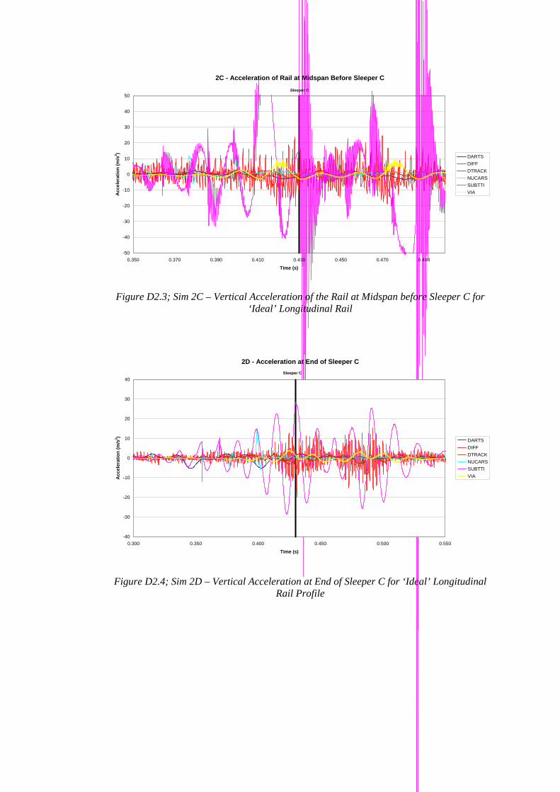
2C - Acceleration of Rail at Midspan Before Sleeper C
-50
-40
-30
-20
-10
0
10
20
30
40
50
0.350 0.370 0.390 0.410 0.430 0.450 0.470 0.490
Time (s)
Acc
eler
atio
n (m
/s2 )
DARTSDIFFDTRACKNUCARSSUBTTIVIA
Sleeper C
Figure D2.3; Sim 2C – Vertical Acceleration of the Rail at Midspan before Sleeper C for ‘Ideal’ Longitudinal Rail
2D - Acceleration at End of Sleeper C
-40
-30
-20
-10
0
10
20
30
40
0.300 0.350 0.400 0.450 0.500 0.550
Time (s)
Acc
eler
atio
n (m
/s2 )
DARTSDIFFDTRACKNUCARSSUBTTIVIA
Sleeper C
Figure D2.4; Sim 2D – Vertical Acceleration at End of Sleeper C for ‘Ideal’ Longitudinal Rail Profile

2E - Acceleration at Mid Span of Sleeper C
-40
-30
-20
-10
0
10
20
30
40
0.300 0.350 0.400 0.450 0.500 0.550
Time (s)
Acc
eler
atio
n (m
/s2 )
DARTSDIFFDTRACKNUCARSSUBTTIVIA
Sleeper C
Figure D2.5; Sim 2E – Vertical Acceleration at Mid Span of Sleeper C for ‘Ideal’ Longitudinal Rail Profile
2F - Bending Moment at Rail Seat of Sleeper C
-4.0
-2.0
0.0
2.0
4.0
6.0
8.0
0.200 0.250 0.300 0.350 0.400 0.450 0.500 0.550 0.600 0.650 0.700
Time (s)
Ben
ding
Mom
ent (
kNm
)
DARTSDIFFDTRACKNUCARSSUBTTIVIA
Sleeper C
Figure D2.6; Sim 2F – Sleeper Bending Moment at Rail Seat for ‘Ideal’ Longitudinal Rail Profile

2G - Bending Moment at Midspan of Sleeper C
-5.5
-5.0
-4.5
-4.0
-3.5
-3.0
-2.5
-2.0
-1.5
-1.0
-0.5
0.0
0.5
1.0
1.5
2.0
2.5
3.0
3.5
0.150 0.250 0.350 0.450 0.550 0.650 0.750
Time (s)
Ben
ding
Mom
ent (
kNm
)
DARTSDIFFDTRACKNUCARSSUBTTIVIA
Sleeper C
Figure D2.7; Sim 2G – Sleeper Bending Moment at Centre for ‘Ideal’ Longitudinal Rail Profile

Appendix D3 Simulation 3 RKWF Wagon 28t at 75.0km/hr Ideal Longitudinal Rail Profile
3A - Normal Contact Force Between Wheel and Rail
20
25
30
35
40
45
50
0.400 0.450 0.500 0.550 0.600 0.650 0.700
Time (s)
Con
tact
For
ce (k
N)
DARTSDIFFDTRACKNUCARSSUBTTIVIA
Sleeper C
Figure D3.1; Sim 3A – Wheel/Rail Contact Force for Leading Wheel for ‘Ideal’ Longitudinal Rail
3B - Shear Force in Rail at Midspan Before Sleeper C
-25
-20
-15
-10
-5
0
5
10
15
20
25
0.350 0.400 0.450 0.500 0.550 0.600 0.650 0.700 0.750 0.800
Time (s)
Shea
r For
ce (k
N) DARTS
DIFFDTRACKNUCARSSUBTTIVIA
Sleeper C
Figure D3.2; Sim 3B – Shear Force in Rail for ‘Ideal’ Longitudinal Rail

3C - Acceleration of Rail at Midspan Before Sleeper C
-50
-40
-30
-20
-10
0
10
20
30
40
50
0.400 0.450 0.500 0.550 0.600 0.650 0.700
Time (s)
Acc
eler
atio
n (m
/s2 )
DARTSDIFFDTRACKNUCARSSUBTTIVIA
Sleeper C
Figure D3.3; Sim 3C – Vertical Acceleration of the Rail at Midspan before Sleeper C for ‘Ideal’ Longitudinal Rail
3D - Acceleration at End of Sleeper C
-60
-50
-40
-30
-20
-10
0
10
20
30
0.224 0.324 0.424 0.524 0.624 0.724
Time (s)
Acc
eler
atio
n (m
/s2 )
DARTSDIFFDTRACKNUCARSSUBTTIVIA
Sleeper C
Figure D3.4; Sim 3D – Vertical Acceleration at End of Sleeper C for ‘Ideal’ Longitudinal Rail Profile

3E - Acceleration at Mid Span of Sleeper C
-10
-8
-6
-4
-2
0
2
4
6
8
10
0.25 0.35 0.45 0.55 0.65 0.75 0.85
Time (s)
Acc
eler
atio
n (m
/s2 )
DARTSDIFFDTRACKNUCARSSUBTTIVIA
Sleeper C
Figure D3.5; Sim 3E – Vertical Acceleration at Mid Span of Sleeper C for ‘Ideal’ Longitudinal Rail Profile
3F - Bending Moment at Rail Seat of Sleeper C
-2.0
-1.0
0.0
1.0
2.0
3.0
4.0
5.0
0.200 0.300 0.400 0.500 0.600 0.700 0.800
Time (s)
Ben
ding
Mom
ent (
kNm
)
DARTSDIFFDTRACKNUCARSSUBTTIVIA
Sleeper C
Figure D3.6; Sim 3F – Sleeper Bending Moment at Rail Seat for ‘Ideal’ Longitudinal Rail Profile

3G - Bending Moment at Midspan of Sleeper C
-6.5
-6.0
-5.5
-5.0
-4.5
-4.0
-3.5
-3.0
-2.5
-2.0
-1.5
-1.0
-0.5
0.0
0.5
1.0
1.5
0.150 0.250 0.350 0.450 0.550 0.650 0.750
Time (s)
Ben
ding
Mom
ent (
kNm
)
DARTSDIFFDTRACKNUCARSSUBTTIVIA
Sleeper C
Figure D3.7; Sim 3G – Sleeper Bending Moment at Centre for ‘Ideal’ Longitudinal Rail Profile

Appendix D4 Simulation 4 RKWF Wagon 100t at 83.1km/hr Ideal Longitudinal Rail Profile
4A - Normal Contact Force Between Wheel and Rail
80
90
100
110
120
130
140
150
160
170
0.300 0.350 0.400 0.450 0.500 0.550 0.600 0.650 0.700
Time (s)
Con
tact
For
ce (k
N)
DARTSDIFFDTRACKNUCARSSUBTTIVIA
Sleeper C
Figure D4.1; Sim 4A – Wheel/Rail Contact Force for Leading Wheel for ‘Ideal’ Longitudinal Rail
4B - Shear Force in Rail at Midspan Before Sleeper C
-80
-60
-40
-20
0
20
40
60
80
0.350 0.400 0.450 0.500 0.550 0.600 0.650 0.700
Time (s)
Shea
r For
ce (k
N) DARTS
DIFFDTRACKNUCARSSUBTTIVIA
Sleeper C
Figure D4.2; Sim 4B – Shear Force in Rail for ‘Ideal’ Longitudinal Rail

4C - Acceleration of Rail at Midspan Before Sleeper C
-50
-40
-30
-20
-10
0
10
20
30
40
50
0.400 0.420 0.440 0.460 0.480 0.500 0.520 0.540 0.560 0.580 0.600
Time (s)
Acc
eler
atio
n (m
/s2 )
DARTSDIFFDTRACKNUCARSSUBTTIVIA
Sleeper C
Figure D4.3; Sim 4C – Vertical Acceleration of the Rail at Midspan before Sleeper C for ‘Ideal’ Longitudinal Rail
4D - Acceleration at End of Sleeper C
-60
-50
-40
-30
-20
-10
0
10
20
30
40
0.200 0.300 0.400 0.500 0.600 0.700 0.800
Time (s)
Acc
eler
atio
n (m
/s2 )
DARTSDIFFDTRACKNUCARSSUBTTIVIA
Sleeper C
Figure D4.4; Sim 4D – Vertical Acceleration at End of Sleeper C for ‘Ideal’ Longitudinal Rail Profile

4E - Acceleration at Mid Span of Sleeper C
-40
-30
-20
-10
0
10
20
30
40
0.250 0.300 0.350 0.400 0.450 0.500 0.550 0.600 0.650 0.700
Time (s)
Acc
eler
atio
n (m
/s2 )
DARTSDIFFDTRACKNUCARSSUBTTIVIA
Sleeper C
Figure D4.5; Sim 4E – Vertical Acceleration at Mid Span of Sleeper C for ‘Ideal’ Longitudinal Rail Profile
4F - Bending Moment at Rail Seat of Sleeper C
-4.0
-2.0
0.0
2.0
4.0
6.0
8.0
10.0
0.250 0.300 0.350 0.400 0.450 0.500 0.550 0.600 0.650 0.700
Time (s)
Ben
ding
Mom
ent (
kNm
)
DARTSDIFFDTRACKNUCARSSUBTTIVIA
Sleeper C
Figure D4.6; Sim 4F – Sleeper Bending Moment at Rail Seat for ‘Ideal’ Longitudinal Rail Profile

4G - Bending Moment at Midspan of Sleeper C
-7.0
-6.0
-5.0
-4.0
-3.0
-2.0
-1.0
0.0
1.0
2.0
3.0
4.0
5.0
0.150 0.250 0.350 0.450 0.550 0.650 0.750
Time (s)
Ben
ding
Mom
ent (
kNm
)
DARTSDIFFDTRACKNUCARSSUBTTIVIA
Sleeper C
Figure D4.7; Sim 4G – Sleeper Bending Moment at Centre for ‘Ideal’ Longitudinal Rail Profile
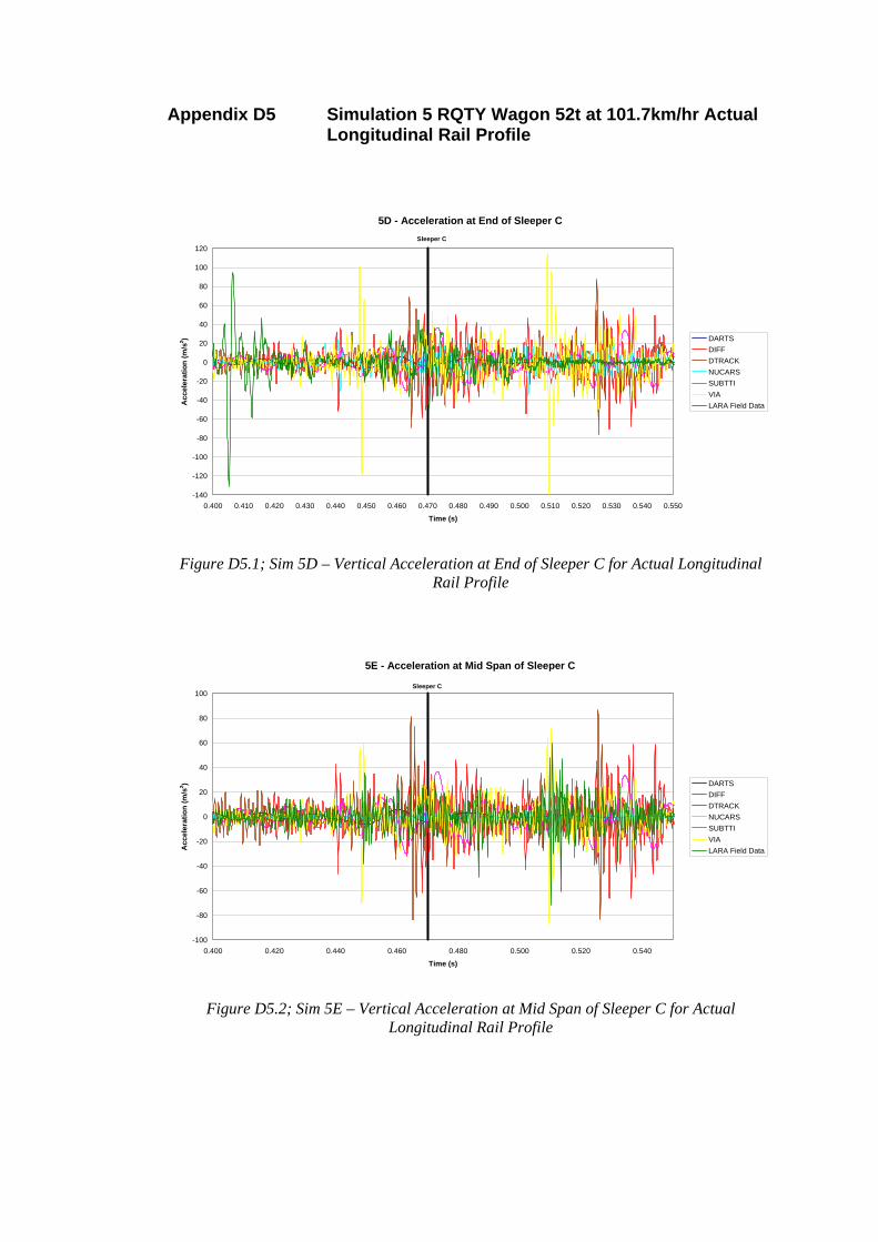
Appendix D5 Simulation 5 RQTY Wagon 52t at 101.7km/hr Actual Longitudinal Rail Profile
5D - Acceleration at End of Sleeper C
-140
-120
-100
-80
-60
-40
-20
0
20
40
60
80
100
120
0.400 0.410 0.420 0.430 0.440 0.450 0.460 0.470 0.480 0.490 0.500 0.510 0.520 0.530 0.540 0.550
Time (s)
Acc
eler
atio
n (m
/s2 ) DARTS
DIFFDTRACKNUCARSSUBTTIVIALARA Field Data
Sleeper C
Figure D5.1; Sim 5D – Vertical Acceleration at End of Sleeper C for Actual Longitudinal Rail Profile
5E - Acceleration at Mid Span of Sleeper C
-100
-80
-60
-40
-20
0
20
40
60
80
100
0.400 0.420 0.440 0.460 0.480 0.500 0.520 0.540
Time (s)
Acc
eler
atio
n (m
/s2 ) DARTS
DIFFDTRACKNUCARSSUBTTIVIALARA Field Data
Sleeper C
Figure D5.2; Sim 5E – Vertical Acceleration at Mid Span of Sleeper C for Actual Longitudinal Rail Profile

Appendix D6 Simulation 6 RQTY Wagon 78t at 110.8km/hr Actual Longitudinal Rail Profile
6A - Normal Contact Force Between Wheel and Rail
-40
-30
-20
-10
0
10
20
30
40
50
60
70
80
90
100
110
120
130
140
150
0.259 0.309 0.359 0.409 0.459 0.509 0.559
Time (s)
Con
tact
For
ce (k
N)
-5
0
5
10
15
20D
epth (mm
)
DARTSDIFFDTRACKNUCARSSUBTTIVIAProfile 1, To Melbourne
Sleeper C
Figure D6.1; Sim 6A – Wheel/Rail Contact Force for Leading Wheel for Actual Longitudinal
Rail
6B - Shear Force in Rail at Midspan Before Sleeper C
-80
-60
-40
-20
0
20
40
60
80
100
120
0.350 0.400 0.450 0.500 0.550
Time (s)
Shea
r For
ce (k
N) DARTS
DIFFDTRACKNUCARSSUBTTIVIALARA Field Data
Sleeper C
Figure D6.2; Sim 6B – Shear Force in Rail for Actual Longitudinal Rail

6C - Acceleration of Rail at Midspan Before Sleeper C
-1500
-1000
-500
0
500
1000
1500
0.300 0.350 0.400 0.450 0.500 0.550
Time (s)
Acc
eler
atio
n (m
/s2 ) DARTS
DIFFDTRACKNUCARSSUBTTIVIALARA Field Data
Sleeper C
Figure D6.3; Sim 6C – Vertical Acceleration of the Rail at Midspan before Sleeper C for Actual Longitudinal Rail
6D - Acceleration at End of Sleeper C
-400
-300
-200
-100
0
100
200
300
400
0.350 0.400 0.450 0.500 0.550
Time (s)
Acc
eler
atio
n (m
/s2 ) DARTS
DIFFDTRACKNUCARSSUBTTIVIALARA Field Data
Sleeper C
Figure D6.4; Sim 6D – Vertical Acceleration at End of Sleeper C for Actual Longitudinal Rail Profile

6E - Acceleration at Mid Span of Sleeper C
-150
-100
-50
0
50
100
150
0.300 0.350 0.400 0.450 0.500 0.550
Time (s)
Acc
eler
atio
n (m
/s2 ) DARTS
DIFFDTRACKNUCARSSUBTTIVIALARA Field Data
Sleeper C
Figure D6.5; Sim 6E – Vertical Acceleration at Mid Span of Sleeper C for Actual Longitudinal Rail Profile
6F - Bending Moment at Rail Seat of Sleeper C
-6.0
-4.0
-2.0
0.0
2.0
4.0
6.0
8.0
10.0
0.200 0.250 0.300 0.350 0.400 0.450 0.500 0.550 0.600 0.650 0.700
Time (s)
Ben
ding
Mom
ent (
kNm
)
DARTSDIFFDTRACKNUCARSSUBTTIVIALARA Field Data
Sleeper C
Figure D6.6; Sim 6F – Sleeper Bending Moment at Rail Seat for Actual Longitudinal Rail Profile

6G - Bending Moment at Midspan of Sleeper C
-7.0
-6.0
-5.0
-4.0
-3.0
-2.0
-1.0
0.0
1.0
2.0
3.0
4.0
0.150 0.250 0.350 0.450 0.550 0.650 0.750
Time (s)
Ben
ding
Mom
ent (
kNm
)
DARTSDIFFDTRACKNUCARSSUBTTIVIALARA Field Data
Sleeper C
Figure D6.7; Sim 6G – Sleeper Bending Moment at Centre for Actual Longitudinal Rail Profile

Appendix D7 Simulation 7 RKWF Wagon 28t at 75.0km/hr Actual Longitudinal Rail Profile
7A - Normal Contact Force Between Wheel and Rail
-40
-30
-20
-10
0
10
20
30
40
50
60
70
80
0.300 0.350 0.400 0.450 0.500 0.550 0.600 0.650 0.700 0.750 0.800
Time (s)
Con
tact
For
ce (k
N)
-5
0
5
10
15
20
Depth (m
m)
DARTSDIFFDTRACKNUCARSSUBTTIVIAProfile 2, To Geelong
Sleeper C
Figure D7.1; Sim 7A – Wheel/Rail Contact Force for Leading Wheel for Actual Longitudinal
Rail
7B - Shear Force in Rail at Midspan Before Sleeper C
-30
-20
-10
0
10
20
30
40
50
0.450 0.500 0.550 0.600 0.650 0.700 0.750
Time (s)
Shea
r For
ce (k
N) DARTS
DIFFDTRACKNUCARSSUBTTIVIALARA Field Data
Sleeper C
Figure D7.2; Sim 7B – Shear Force in Rail for Actual Longitudinal Rail
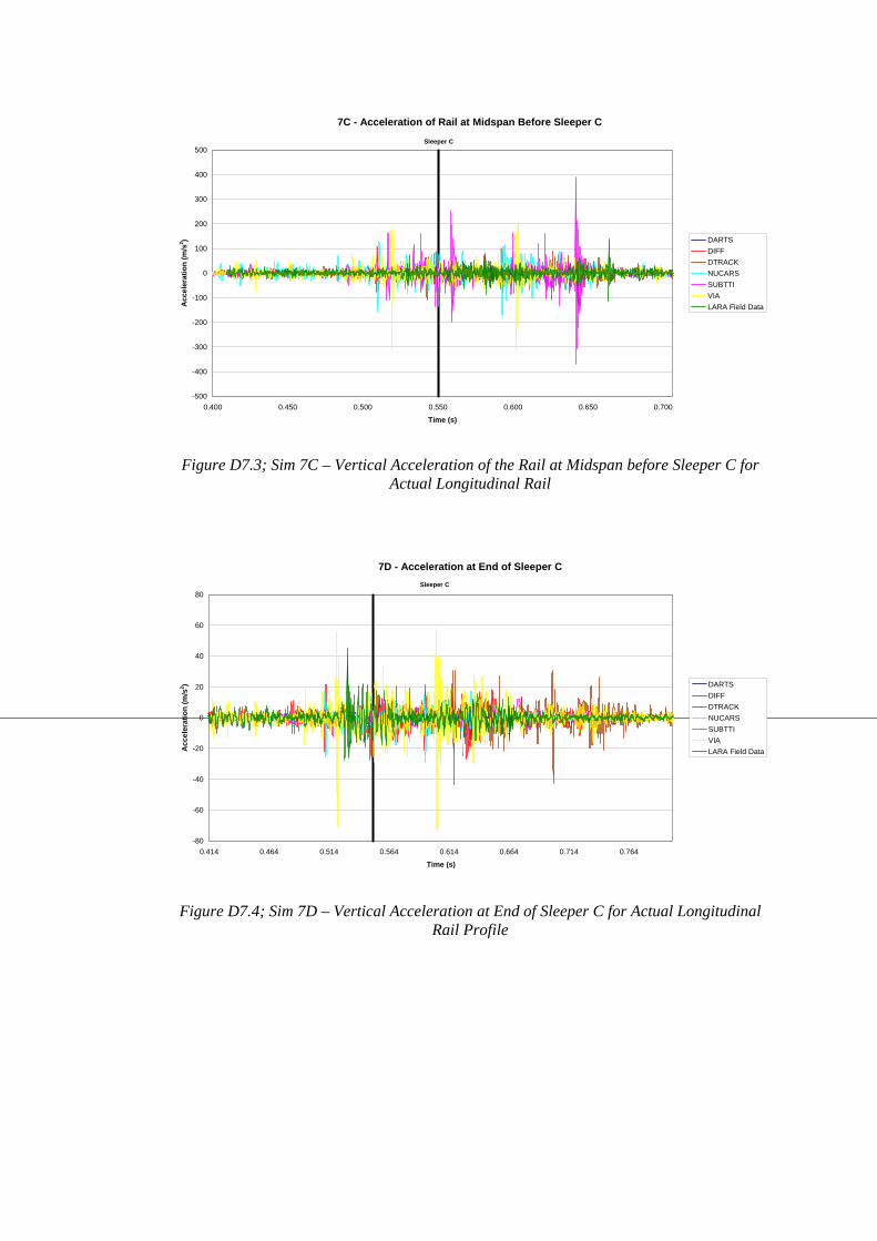
7C - Acceleration of Rail at Midspan Before Sleeper C
-500
-400
-300
-200
-100
0
100
200
300
400
500
0.400 0.450 0.500 0.550 0.600 0.650 0.700
Time (s)
Acc
eler
atio
n (m
/s2 ) DARTS
DIFFDTRACKNUCARSSUBTTIVIALARA Field Data
Sleeper C
Figure D7.3; Sim 7C – Vertical Acceleration of the Rail at Midspan before Sleeper C for Actual Longitudinal Rail
7D - Acceleration at End of Sleeper C
-80
-60
-40
-20
0
20
40
60
80
0.414 0.464 0.514 0.564 0.614 0.664 0.714 0.764
Time (s)
Acc
eler
atio
n (m
/s2 ) DARTS
DIFFDTRACKNUCARSSUBTTIVIALARA Field Data
Sleeper C
Figure D7.4; Sim 7D – Vertical Acceleration at End of Sleeper C for Actual Longitudinal Rail Profile

7E - Acceleration at Mid Span of Sleeper C
-80
-60
-40
-20
0
20
40
60
80
0.400 0.450 0.500 0.550 0.600 0.650 0.700
Time (s)
Acc
eler
atio
n (m
/s2 ) DARTS
DIFFDTRACKNUCARSSUBTTIVIALARA Field Data
Sleeper C
Figure D7.5; Sim 7E – Vertical Acceleration at Mid Span of Sleeper C for Actual Longitudinal Rail Profile
7F - Bending Moment at Rail Seat of Sleeper C
-2.0
-1.0
0.0
1.0
2.0
3.0
4.0
5.0
0.200 0.300 0.400 0.500 0.600 0.700 0.800
Time (s)
Ben
ding
Mom
ent (
kNm
)
DARTSDIFFDTRACKNUCARSSUBTTIVIALARA Field Data
Sleeper C
Figure D7.6; Sim 7F – Sleeper Bending Moment at Rail Seat for Actual Longitudinal Rail Profile

7G - Bending Moment at Midspan of Sleeper C
-3.5
-3.0
-2.5
-2.0
-1.5
-1.0
-0.5
0.0
0.5
1.0
1.5
2.0
0.250 0.350 0.450 0.550 0.650 0.750 0.850
Time (s)
Ben
ding
Mom
ent (
kNm
)
DARTSDIFFDTRACKNUCARSSUBTTIVIALARA Field Data
Sleeper C
Figure D7.7; Sim 7G – Sleeper Bending Moment at Centre for Actual Longitudinal Rail Profile

Appendix D8 Simulation 8 RKWF Wagon 100t at 83.1km/hr Actual Longitudinal Rail Profile
8A - Normal Contact Force Between Wheel and Rail
0
10
20
30
40
50
60
70
80
90
100
110
120
130
140
150
160
170
180
0.300 0.350 0.400 0.450 0.500 0.550 0.600 0.650 0.700
Time (s)
Con
tact
For
ce (k
N)
-5
0
5
10
15
20D
epth (mm
)
DARTSDIFFDTRACKNUCARSSUBTTIVIAProfile 1, To Melbourne
Sleeper C
Figure D8.1; Sim 8A – Wheel/Rail Contact Force for Leading Wheel for Actual Longitudinal
Rail
8B - Shear Force in Rail at Midspan Before Sleeper C
-100
-50
0
50
100
150
0.400 0.450 0.500 0.550 0.600 0.650
Time (s)
Shea
r For
ce (k
N) DARTS
DIFFDTRACKNUCARSSUBTTIVIALARA Field Data
Sleeper C
Figure D8.2; Sim 8B – Shear Force in Rail for Actual Longitudinal Rail

8C - Acceleration of Rail at Midspan Before Sleeper C
-2000
-1500
-1000
-500
0
500
1000
1500
2000
0.450 0.470 0.490 0.510 0.530 0.550
Time (s)
Acc
eler
atio
n (m
/s2 ) DARTS
DIFFDTRACKNUCARSSUBTTIVIALARA Field Data
Sleeper C
Figure D8.3; Sim 8C – Vertical Acceleration of the Rail at Midspan before Sleeper C for Actual Longitudinal Rail
8D - Acceleration at End of Sleeper C
-120
-100
-80
-60
-40
-20
0
20
40
60
80
100
0.200 0.300 0.400 0.500 0.600 0.700 0.800
Time (s)
Acc
eler
atio
n (m
/s2 ) DARTS
DIFFDTRACKNUCARSSUBTTIVIALARA Field Data
Sleeper C
Figure D8.4; Sim 8D – Vertical Acceleration at End of Sleeper C for Actual Longitudinal Rail Profile

8E - Acceleration at Mid Span of Sleeper C
-80
-60
-40
-20
0
20
40
60
0.350 0.400 0.450 0.500 0.550 0.600 0.650
Time (s)
Acc
eler
atio
n (m
/s2 ) DARTS
DIFFDTRACKNUCARSSUBTTIVIALARA Field Data
Sleeper C
Figure D8.5; Sim 8E – Vertical Acceleration at Mid Span of Sleeper C for Actual Longitudinal Rail Profile
8F - Bending Moment at Rail Seat of Sleeper C
-6.0
-4.0
-2.0
0.0
2.0
4.0
6.0
8.0
10.0
12.0
0.200 0.250 0.300 0.350 0.400 0.450 0.500 0.550 0.600 0.650 0.700
Time (s)
Ben
ding
Mom
ent (
kNm
)
DARTSDIFFDTRACKNUCARSSUBTTIVIALARA Field Data
Sleeper C
Figure D8.6; Sim 8F – Sleeper Bending Moment at Rail Seat for Actual Longitudinal Rail Profile

8G - Bending Moment at Midspan of Sleeper C
-8.0
-7.0
-6.0
-5.0
-4.0
-3.0
-2.0
-1.0
0.0
1.0
2.0
3.0
4.0
5.0
0.150 0.250 0.350 0.450 0.550 0.650 0.750
Time (s)
Ben
ding
Mom
ent (
kNm
)
DARTSDIFFDTRACKNUCARSSUBTTIVIALARA Field Data
Sleeper C
Figure D8.7; Sim 8G – Sleeper Bending Moment at Centre for Actual Longitudinal Rail Profile

Appendix E Summary of Benchmark Output Parameters Results for all Simulations

Table E1 Summary of Max/Min Output Results from Simulation 1
OU
TPU
T
PAR
AM
ET
ER
DA
RT
S
DIF
F
DT
RA
CK
NU
CA
RST
M
SUB
TT
I
VIA
Max (kN) 67.49 65.01 76.54 63.99 84.02 65.87
Avg (kN) 65.03 63.76 65.65 63.70 62.69 63.75 A
Min (kN) 62.46 61.89 58.87 63.14 41.37 61.63
31.18 30.43 14.53 34.15 22.19 28.69 B (kN)
-31.29 -33.04 -14.88 -34.17 -30.45 -28.50
1.58 18.33 5.12 6.04 496.10 3.97 C (m/s2)
-1.94 -12.70 -6.94 -3.37 -412.04 -1.79
9.06 9.06 1.35 9.89 24.70 1.98 D (m/s2)
-12.32 -12.32 -4.35 -3.19 -51.77 -1.19
1.25 11.53 0.97 12.59 24.70 1.59 E (m/s2)
-2.94 -10.56 -2.52 -4.46 -51.77 -1.19
2.21 3.32 3.96 4.70 4.47 2.12 F (kNm)
-0.09 -0.14 -1.70 -0.03 -0.14 -0.09
0.12 0.12 1.87 1.02 0.01 0.14 G (kNm)
-3.12 -3.02 -2.86 -1.27 -0.34 -3.09

Table E2 Summary of Max/Min Output Results from Simulation 2
OU
TPU
T
PAR
AM
ET
ER
DA
RT
S
DIF
F
DT
RA
CK
NU
CA
RST
M
SUB
TT
I
VIA
Max (kN) 101.77 97.44 100.09 95.89 126.94 99.72
Avg (kN) 97.55 95.64 95.66 95.54 94.01 95.62 A
Min (kN) 93.54 92.50 87.23 94.69 61.05 91.56
46.56 45.76 21.82 51.15 34.46 42.64 B (kN)
-46.49 -49.78 -22.43 -58.37 -52.70 -43.11
2.63 24.59 8.40 12.47 1063.15 9.47 C (m/s2)
-3.11 -20.35 -9.47 -6.08 -938.72 -3.31
2.21 15.20 2.29 16.79 28.53 4.02 D (m/s2)
-5.35 -20.04 -8.24 -5.89 -51.70 -2.37
2.08 18.55 1.69 21.32 28.53 3.31 E (m/s2)
-5.01 -15.21 -4.78 -7.78 -51.70 -2.13
3.31 4.96 5.97 7.05 6.79 3.23 F (kNm)
-0.13 -0.21 -2.56 -0.05 -0.28 -0.15
0.19 0.18 2.81 1.76 0.02 0.21 G (kNm)
-4.68 -4.53 -4.33 -1.90 -0.52 -4.71
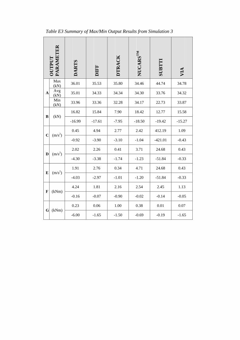
Table E3 Summary of Max/Min Output Results from Simulation 3
OU
TPU
T
PAR
AM
ET
ER
DA
RT
S
DIF
F
DT
RA
CK
NU
CA
RST
M
SUB
TT
I
VIA
Max (kN) 36.01 35.53 35.80 34.46 44.74 34.78
Avg (kN) 35.01 34.33 34.34 34.30 33.76 34.32 A
Min (kN) 33.96 33.36 32.28 34.17 22.73 33.87
16.82 15.84 7.90 18.42 12.77 15.58 B (kN)
-16.99 -17.61 -7.95 -18.50 -19.42 -15.27
0.45 4.94 2.77 2.42 412.19 1.09 C (m/s2)
-0.92 -3.90 -3.10 -1.04 -421.01 -0.43
2.02 2.26 0.41 3.71 24.68 0.43 D (m/s2)
-4.30 -3.38 -1.74 -1.23 -51.84 -0.33
1.91 2.76 0.34 4.71 24.68 0.43 E (m/s2)
-4.03 -2.97 -1.01 -1.20 -51.84 -0.33
4.24 1.81 2.16 2.54 2.45 1.13 F (kNm)
-0.16 -0.07 -0.90 -0.02 -0.14 -0.05
0.23 0.06 1.00 0.38 0.01 0.07 G (kNm)
-6.00 -1.65 -1.50 -0.69 -0.19 -1.65

Table E4 Summary of Max/Min Output Results from Simulation 4
OU
TPU
T
PAR
AM
ET
ER
DA
RT
S
DIF
F
DT
RA
CK
NU
CA
RST
M
SUB
TT
I
VIA
Max (kN) 128.75 125.56 131.21 123.03 159.17 124.70
Avg (kN) 125.07 122.60 122.95 122.50 120.57 122.59 A
Min (kN) 121.14 119.58 112.15 121.90 81.56 120.48
59.68 57.70 28.22 65.72 40.30 55.64 B (kN)
-60.29 -63.20 -28.49 -66.19 -69.63 -54.54
2.01 19.21 9.53 8.84 1684.29 5.41 C (m/s2)
-3.68 -16.18 -11.18 -4.04 -1515.99 -2.70
2.02 10.83 1.67 13.47 32.23 1.62 D (m/s2)
-4.30 -15.40 -7.26 -4.50 -51.63 -1.22
1.91 13.19 1.43 17.74 32.23 1.35 E (m/s2)
-4.03 -13.66 -4.30 -5.60 -51.63 -0.95
4.24 6.43 7.72 9.08 8.60 4.04 F (kNm)
-0.16 -0.25 -3.25 -0.06 -0.37 -0.17
0.23 0.23 3.60 1.38 0.03 0.25 G (kNm)
-6.00 -5.86 -5.40 -2.46 -0.66 -5.88

Table E5 Summary of Max/Min Output Results from Simulation 5
OU
TPU
T
PAR
AM
ET
ER
DA
RT
S
DIF
F
DT
RA
CK
NU
CA
RST
M
SUB
TT
I
VIA
LA
RA
Max (kN) 86.41 89.50 95.04 105.10 152.07 91.92 -
Avg (kN) 65.02 63.76 63.75 63.82 62.56 63.70 - A
Min (kN) 45.57 44.80 33.82 25.93 0.00 31.24 -
30.87 29.95 16.65 50.68 18.56 28.49 77.02* B (kN)
-24.65 -38.73 -17.65 -47.88 -41.76 -36.21 -10.55*
13.55 268.78 172.44 246.98 412.88 377.50 379.42 C (m/s2)
-17.96 -179.55 -196.13 -292.23 -285.54 -574.29 -391.13
6.35 57.14 87.15 25.73 36.70 114.66 115.95 D (m/s2)
-6.65 -70.18 -76.65 -35.24 -51.77 -139.85 -159.08
6.00 59.04 86.82 54.98 36.70 72.60 78.23 E (m/s2)
-6.23 -66.31 -82.98 -73.19 -51.77 -87.09 -89.74
2.42 4.42 5.77 6.54 5.38 3.20 1.21 F (kNm)
-0.10 -0.24 -1.74 -0.04 -0.22 -0.25 -0.14
0.14 0.18 2.11 2.26 0.02 0.26 0.05 G (kNm)
-3.42 -4.07 -3.41 -3.07 -0.42 -4.51 -2.92
* the Lara field data collected is not a representation of the shear force in the rail. It is a measure of the wheel/rail force and its (maximum-minimum) value should be equal to the peak change in shear force.

Table E6 Summary of Max/Min Output Results from Simulation 6
OU
TPU
T
PAR
AM
ET
ER
DA
RT
S
DIF
F
DT
RA
CK
NU
CA
RST
M
SUB
TT
I
VIA
LA
RA
Max (kN) 124.41 122.49 141.18 135.09 145.41 130.31 -
Avg (kN) 97.58 95.60 95.64 95.55 94.00 95.61 - A
Min (kN) 73.56 65.02 64.75 38.72 38.30 50.10 -
49.01 46.47 28.30 53.67 35.24 47.12 103.40* B (kN)
-44.84 -52.22 -20.04 -58.42 -56.63 -48.12 -10.55*
10.28 196.87 0.10 356.00 1053.65 330.18 428.24 C (m/s2)
-16.00 -211.70 -239.90 -321.65 -1083.63 -299.41 -534.85
12.02 97.29 67.95 27.87 51.74 95.15 54.47 D (m/s2)
-18.04 -96.75 -74.31 -35.04 -51.70 -131.36 -63.56
11.22 101.30 84.80 84.53 51.74 63.67 58.12 E (m/s2)
-16.95 -92.14 -111.27 -97.80 -51.70 -81.89 -69.62
3.99 5.43 6.73 9.24 7.44 3.92 1.77 F (kNm)
-0.13 -0.27 -3.53 -0.06 -0.31 -0.27 -0.30
0.19 0.23 2.85 2.16 0.02 0.32 0.21 G (kNm)
-5.68 -4.95 -4.27 -3.85 -0.57 -5.61 -3.52
* the Lara field data collected is not a representation of the shear force in the rail. It is a measure of the wheel/rail force and its (maximum-minimum) value should be equal to the peak change in shear force.

Table E7 Summary of Max/Min Output Results from Simulation 7
OU
TPU
T
PAR
AM
ET
ER
DA
RT
S
DIF
F
DT
RA
CK
NU
CA
RST
M
SUB
TT
I
VIA
LA
RA
Max (kN) 55.83 60.55 51.24 64.42 117.24 48.37 -
Avg (kN) 35.01 34.33 34.34 34.33 33.65 34.32 - A
Min (kN) 14.02 9.48 17.16 5.05 0.00 16.12 -
20.49 12.02 8.64 22.08 10.10 16.05 37.98 B (kN)
-11.67 -23.93 -10.20 -25.08 -23.13 -20.61 -9.50
7.63 104.36 89.82 128.76 389.38 210.61 138.64 C (m/s2)
-8.17 -79.94 -110.82 -171.44 -368.68 -313.26 -112.08
3.52 21.73 30.62 16.94 24.68 57.18 44.41 D (m/s2)
-3.94 -27.82 -43.76 -29.36 -51.84 -73.24 -27.53
3.32 19.86 41.96 37.00 24.68 32.34 55.55 E (m/s2)
-3.71 -30.86 -32.67 -53.83 -51.84 -44.60 -63.41
1.37 3.20 3.35 3.98 2.78 1.68 0.23 F (kNm)
-0.05 -0.14 -0.96 -0.09 -0.14 -0.12 -0.55
0.08 0.11 1.21 1.47 0.01 0.13 0.14 G (kNm)
-1.94 -2.91 -2.05 -2.89 -0.21 -2.34 -2.01
* the Lara field data collected is not a representation of the shear force in the rail. It is a measure of the wheel/rail force and its (maximum-minimum) value should be equal to the peak change in shear force.

Table E8 Summary of Max/Min Output Results from Simulation 8
OU
TPU
T
PAR
AM
ET
ER
DA
RT
S
DIF
F
DT
RA
CK
NU
CA
RST
M
SUB
TT
I
VIA
LA
RA
Max (kN) 145.49 146.51 149.67 154.71 169.92 144.25 -
Avg (kN) 125.11 122.60 122.95 122.56 120.48 122.62 - A
Min (kN) 104.55 99.70 103.13 96.32 68.07 97.74 -
63.44 56.57 31.96 75.61 41.70 57.96 127.67 B (kN)
-59.40 -64.28 -28.06 -67.88 -73.36 -54.10 -5.28
5.50 128.01 114.60 209.86 1707.69 215.12 159.15 C (m/s2)
-8.81 -130.83 -132.75 -177.25 -1663.11 -202.54 -136.88
7.72 28.56 36.58 21.96 32.24 71.80 16.64 D (m/s2)
-11.89 -40.23 -29.43 -28.62 -51.63 -99.38 -21.78
7.23 29.21 44.58 50.26 32.24 53.27 28.43 E (m/s2)
-11.18 -38.28 -47.01 -57.00 -51.63 -61.11 -34.77
4.76 7.09 8.66 10.36 8.89 4.53 1.27 F (kNm)
-0.16 -0.30 -3.78 -0.06 -0.39 -0.27 -0.17
0.23 0.26 3.64 1.46 0.03 0.32 0.31 G (kNm)
-6.75 -6.46 -5.28 -3.97 -0.69 -6.48 -3.99
* the Lara field data collected is not a representation of the shear force in the rail. It is a measure of the wheel/rail force and its (maximum-minimum) value should be equal to the peak change in shear force.

Appendix F Drawing of typical concrete sleeper found at Braeside, Drawing Number No 201-05 and calculation of ultimate limit strength